Predicting Minimum Control Speed on the Ground … · 2016-12-01 · 23. Coefficient of Drag (CD)...

Predicting Minimum Control Speed on the Ground (VMCG) and Minimum Control

Airspeed (VMCA) of Engine Inoperative Flight Using Aerodynamic Database and

Propulsion Database Generators

by

Eric Michael Hadder

A Thesis Presented in Partial Fulfillment

of the Requirements for the Degree

Master of Science

Approved November 2016 by the

Graduate Supervisory Committee:

Timothy Takahashi, Chair

Marc Mignolet

Daniel White

ARIZONA STATE UNIVERSITY

December 2016

i

ABSTRACT

There are many computer aided engineering tools and software used by aerospace

engineers to design and predict specific parameters of an airplane. These tools help a

design engineer predict and calculate such parameters such as lift, drag, pitching moment,

takeoff range, maximum takeoff weight, maximum flight range and much more.

However, there are very limited ways to predict and calculate the minimum control

speeds of an airplane in engine inoperative flight. There are simple solutions, as well as

complicated solutions, yet there is neither standard technique nor consistency throughout

the aerospace industry. To further complicate this subject, airplane designers have the

option of using an Automatic Thrust Control System (ATCS), which directly alters the

minimum control speeds of an airplane.

This work addresses this issue with a tool used to predict and calculate the

Minimum Control Speed on the Ground (VMCG) as well as the Minimum Control

Airspeed (VMCA) of any existing or design-stage airplane. With simple line art of an

airplane, a program called VORLAX is used to generate an aerodynamic database used to

calculate the stability derivatives of an airplane. Using another program called Numerical

Propulsion System Simulation (NPSS), a propulsion database is generated to use with the

aerodynamic database to calculate both VMCG and VMCA.

This tool was tested using two airplanes, the Airbus A320 and the Lockheed

Martin C130J-30 Super Hercules. The A320 does not use an Automatic Thrust Control

System (ATCS), whereas the C130J-30 does use an ATCS. The tool was able to properly

ii

calculate and match known values of VMCG and VMCA for both of the airplanes. The

fact that this tool was able to calculate the known values of VMCG and VMCA for both

airplanes means that this tool would be able to predict the VMCG and VMCA of an

airplane in the preliminary stages of design. This would allow design engineers the ability

to use an Automatic Thrust Control System (ATCS) as part of the design of an airplane

and still have the ability to predict the VMCG and VMCA of the airplane.

iii

DEDICATION

In loving memory of my beautiful and supportive mother.

iv

ACKNOWLEDGMENTS

This thesis derives from work funded by DragonFly Aeronautics LLC under

Contract No. FP00006911.

v

TABLE OF CONTENTS

Page

LIST OF TABLES ............................................................................................................. vi

LIST OF FIGURES ........................................................................................................... ix

CHAPTER

1 INTRODUCTION ......................................................................................1

2 METHOD ..................................................................................................11

3 AERODYNAMIC DATABASE GENERATOR ......................................14

4 COMPUTING MINIMUM CCONTROL SPEED ON THE GROUND

(VMCG) .....................................................................................................28

5 COMPUTING MINIMUM CONTROL AIRSPEED (VMCA) ................34

6 CALIBRATION OF TEST CASES ........................................................44

7 MORE SOPHISTICATED TRADES ......................................................67

8 MINIMUM CCONTROL AIRSPEED FLIGHT CONFIGURATION

OBSERVATIONS ....................................................................................91

9 CONCLUSION .....................................................................................118

REFERENCES ................................................................................................................121

vi

LIST OF TABLES

Table Page

1. Flight Configurations for the VMCA Solutions Found at Altitude of 0 Ft, Weight of

93,500 Lbm and Sideslip Angle (β) of -3° for A320 ........................................................ 92


128,500 Lbm and Sideslip Angle (β) of -3° for A320 ...................................................... 93


173,500 Lbm and Sideslip Angle (β) of -3° for A320 ...................................................... 94

4. Flight Configurations for the VMCA Solutions Found at Altitude of 6,000 Ft, Weight

of 93,500 Lbm and Sideslip Angle (β) of -3° for A320 .................................................... 95


of 128,500 Lbm and Sideslip Angle (β) of -3° for A320 .................................................. 96


of 173,500 Lbm and Sideslip Angle (β) of -3° for A320 .................................................. 97


75,600 Lbm and Sideslip Angle (β) of -3° for C130J-30-30 ............................................ 98


120,600 Lbm and Sideslip Angle (β) of -3° for C130J-30-30 .......................................... 99


165,600 Lbm and Sideslip Angle (β) of -3° for C130J-30 ............................................. 100


of 75,600 Lbm and Sideslip Angle (β) of -3° for C130J-30-30 ...................................... 101

vii

Table Page


of 120,600 Lbm and Sideslip Angle (β) of -3° for C130J-30-30 .................................... 102


of 165,600 Lbm and Sideslip Angle (β) of -3° for C130J-30 ......................................... 103


93,500 Lbm and Sideslip Angle (β) of 2° for A320 ....................................................... 105


128,500 Lbm and Sideslip Angle (β) of 2° for A320 ..................................................... 106


173,500 Lbm and Sideslip Angle (β) of 2° for A320 ..................................................... 107


of 93,500 Lbm and Sideslip Angle (β) of 2° for A320 ................................................... 108


of 128,500 Lbm and Sideslip Angle (β) of 2° for A320 ................................................. 109


of 173,500 Lbm and Sideslip Angle (β) of 2° for A320 ................................................. 110


75,600 lLbm and Sideslip Angle (β) of 2° for C130J-30 ................................................ 111


120,600 Lbm and Sideslip Angle (β) of 2° for C130J-30 ............................................... 112


165,600 Lbm and Sideslip Angle (β) of 2° for C130J-30 ............................................... 113

viii

Table Page


of 75,600 Lbm and Sideslip Angle (β) of 2° for C130J-30 ............................................ 114


of 120,600 Lbm and Sideslip Angle (β) of 2° for C130J-30 .......................................... 115


of 165,600 Lbm and Sideslip Angle (β) of 2° for C130J-30 .......................................... 116

ix

LIST OF FIGURES

Figure Page

1. Diagram of a Trimmed Airplane .................................................................................. 3

2. Demonstration of x, y and z Axes, as Well as the Pitching, Yawing and Rolling

Moments ............................................................................................................................. 7

3. 5-column Data ............................................................................................................ 13

4. Continuation of Figure 3 ............................................................................................ 13

5. Flowchart of Main Algorithm .................................................................................... 14

6. Master EXCEL Input Example Using C130J-30 Inputs ............................................ 16

7. Continuation of Figure 6 ............................................................................................. 17

8. Continuation of Figure 6 ............................................................................................ 17

9. Oblique View of "panels" Glued Together with Control Surfaces at Maximum

Deflection .......................................................................................................................... 17

10. Formatted Input File for VORLAX Using C130J-30 Inputs .................................... 18

11. Imported Vorlax Output into EXCEL Using C130J-30 Inputs ................................ 22

12. Recorded Stability Derivatives in EXCEL Using C130J-30 Inputs ......................... 25

13. Force Balance for Simplified VMCG Computation ................................................. 29

14. Flowchart of Solving for VMCG .............................................................................. 30

15. Flowchart of Colving for VMCA ............................................................................. 35

16. Algorithm Used to Satisfy the Three Trim Equations .............................................. 36

17. Force and Yawing Moment Balance for Calculating VMCA .................................. 39

18. Side Force Balance for Calculating VMCA ............................................................. 40

19. Rolling Moment Balance for Calculating VMCA .................................................... 40

x

Figure Page

20. Line Art of Airbus A320 ........................................................................................... 44

21. Isometric View of the A320 Represented by 15 Geometric Panels .......................... 45

22. Coefficient of Lift (CL) Vs Angle of Attack (α) for A320 (Takeoff Flaps) ............. 46

23. Coefficient of Drag (CD) Vs Coefficient of Lift (CL) for A320 (Takeoff Flaps) .... 46

24. Pitching Moment Coefficient (Cm) Vs Coefficient of Lift (CL) for A320 (Takeoff

Flaps)................................................................................................................................. 47

25. δCn/δβ Vs Angle of Attack (α) for A320 ................................................................. 48

26. δCl/δβ Vs Angle of Attack (α) for A320 .................................................................. 48

27. δCY/δβ Vs Angle of Attack (α) for A320................................................................. 48

28. δCn/δθaileron Vs Angle of Attack (α) for A320 ...................................................... 49

29. δCl/δθaileron Vs Angle of Attack (α) for A320 ....................................................... 49

30. δCY/δθaileron Vs Angle of Attack (α) for A320...................................................... 49

31. δCn/δθrudder Vs Angle of Attack (α) for A320 ....................................................... 50

32. δCl/δθrudder Vs Angle of Attack (α) for A320 ........................................................ 50

33. δCY/δθrudder Vs Angle of Attack (α) for A320 ...................................................... 50

34. Vietnam Airline A320 Performance Book Values for V2 and V1 ........................... 52

35. Vietnam Airline A320 “Comparable VMCG” Vs Altitude of A320 ........................ 52

36. VMCG Vs Altitude at Five Different Temperatures for A320 ................................. 53

37. VMCG Vs Temperature at Six Different Altitudes for A320................................... 53

38. VMCA Vs Weight at “Worse Case” Temperature” ................................................. 54

39. VMCA Vs Weight at T = ISA -20 for A320 ............................................................ 55

40. Line Art of Lockheed Martin C130J-30 Super Hercules .......................................... 56

xi

Figure Page

41. Isometric View of the C130J-30 Represented by 14 Geometric Panels ................... 57

42. Coefficient of Lift (CL) Vs Angle of Attack (α) for C130J-30 (Takeoff Flaps) ...... 58

43. Coefficient of Drag (CD) Vs Coefficient of Lift (CL) for C130J-30 (Takeoff

Flaps)................................................................................................................................. 58

44. Pitching Moment Coefficient (Cm) Vs Coefficient of Lift (CL) for C130J-30

(Takeoff Flaps).................................................................................................................. 59

45. δCn/δβ Vs Angle of Attack (α) for C130J-30 ........................................................... 60

46. δCl/δβ Vs Angle of Attack (α) for C130J-30 ............................................................ 60

47. δCY/δβ Vs Angle of Attack (α) for C130J-30 .......................................................... 60

48. δCn/δθaileron Vs Angle of Attack (α) for C130J-30 ................................................ 61

49. δCl/δθaileron Vs Angle of Attack (α) for C130J-30 ................................................. 61

50. δCY/δθaileron Vs Angle of Attack (α) for C130J-30 ............................................... 61

51. δCn/δθrudder Vs Angle of Attack (α) for C130J-30 ................................................ 62

52. δCl/δθrudder Vs Angle of Attack (α) for C130J-30 ................................................. 62

53. δCY/δθrudder Vs Angle of Attack (α) for C130J-30 ................................................ 62

54. VMCG Vs Altitude at Five Different Temperatures for C130J-30 .......................... 64

55. VMCG Vs Temperature at Six Different Altitudes for C130J-30 ............................ 64

56. VMCA Vs Weight at T = ISA -20 for C130J-30 ...................................................... 65

57. VMCA Vs Weight at T = ISA and Altitude = Sea Level for A320 .......................... 68

58. VMCA Vs Weight at T = ISA and Altitude = 2,000 Ft for A320 ............................ 68



xii

Figure Page


62. VMCA Vs Weight at T = ISA and Altitude = 10,000 Ft for A320 .......................... 69

63. VMCA Vs Weight at T = ISA and Altitude = 12,000 Ft for A320 .......................... 70

64. VMCA Vs Weight at T = ISA for A320 ................................................................... 70

65. VMCA Vs Weight at T = ISA and Altitude = Sea Level for C130J-30 ................... 71

66. VMCA Vs Weight at T = ISA and Altitude = 2,000 Ft for C130J-30 ...................... 71




70. VMCA Vs Weight at T = ISA and Altitude = 10,000 Ft for C130J-30 .................... 72

71. VMCA Vs Weight at T = ISA and Altitude = 12,000 Ft for C130J-30 .................... 73

72. VMCA Vs Weight at T = ISA for C130J-30 ............................................................ 73

73. Angle of Attack (α) Vs Weight for A320 ................................................................. 74

74. Angle of Attack (α) Vs Weight for C130J-30 ........................................................... 75

75. VMCA Vs Temperature at Light Weight for A320 .................................................. 77

76. VMCA Vs Temperature at Medium Weight for A320 ............................................. 77

77. VMCA Vs Temperature at Heavy Weight for A320 ................................................ 78

78. VMCA Vs Temperature at Light Weight for C130J-30 ........................................... 78

79. VMCA Vs Temperature at Medium Weight for C130J-30 ...................................... 79

80. VMCA Vs Temperature at Heavy Weight for C130J-30 ......................................... 79

81. Angle of Attack (α) Vs Temperature at Light Weight for A320 .............................. 80

82. Angle of Attack (α) Vs Temperature at Medium Weight for A320 ......................... 80

xiii

Figure Page

83. Angle of Attack (α) Vs Temperature at Heavy Weight for A320 ............................ 81

84. Angle of Attack (α) Vs Temperature at Light Weight for C130J-30 ........................ 81

85. Angle of Attack (α) Vs Temperature at Medium Weight for C130J-30 ................... 81

86. Angle of Attack (α) Vs Temperature at Heavy Weight for C130J-30 ...................... 82

87. VMCA Vs Weight at Altitude of Sea Level for A320 ............................................. 83

88. VMCA Vs Weight at Altitude of 6,000 Ft for A320 ................................................ 84

89. VMCA Vs Weight at Altitude of 12,000 Ft for A320 .............................................. 84

90. VMCA Vs Weight at Altitude of Sea Level for C130J-30 ....................................... 85

91. VMCA Vs Weight at Altitude of 6,000 Ft for C130J-30 ......................................... 85

92. VMCA Vs Weight at Altitude of 12,000 Ft for C130J-30 ....................................... 85

93. Angle of Attack (α) Vs Weight at Altitude of Sea Level for A320 .......................... 86

94. Angle of Attack (α) Vs Weight at Altitude of 6,000 Ft for A320 ............................. 87

95. Angle of Attack (α) Vs Weight at Altitude of 12,000 Ft for A320 ........................... 87

96. Angle of Attack (α) Vs Weight at Altitude of Sea Level for C130J-30 ................... 87

97. Angle of Attack (α) Vs Weight at Altitude of 6,000 Ft for C130J-30 ...................... 88

98. Angle of Attack (α) Vs Temperature at Heavy Weight for C130J-30 ...................... 88

1

Chapter 1: Introduction

As a form of travel, airplanes are becoming more and more economically efficient

and safe. A driver of a car needs only to obtain a driver’s license. After receiving this

license, a driver does not need to go through any continual education, drug tests, or

performance tests. Even though a traveler may be an extremely defensive and good

driver, there are many other drivers that are reckless and dangerous. On the other hand, a

pilot must go through rigorous tests, continual education as well as medical and drug tests

to maintain his or her pilot’s licenses. Additionally, every Instruments Flight Rules (IFR)

flight must be approved through Air Traffic Control, a government service provided by

ground-based controllers to help direct the flow of air traffic and avoid collisions. The

airplane itself must also be certified and maintained for it to be approved for flight.

For an airplane to be certified to fly it must go through many inspections and tests

that are mandated by the United States government. These tests and regulations are found

in the Code of Federal Regulations (CFR). The Code of Federal Regulations (CFR) is a

codification of all of the regulations and administrative laws mandated by the Federal

Government. These regulations cover a broad range of subject matter: there are factors of

safety that ensure that each individual part of the airplane structure is multiple times

stronger than the worst case load bearing scenario. The materials used have been

designed to be strong, replaceable, durable, corrosion resistant, etc.

If for any reason there is a failure in the material or parts, there are redundancies

designed to protect the airplane and its passengers. Some of these redundancies are

2

backup systems of the same function, meaning there may be a second computer for each

automated part of the airplane that will override the original if there is a system error, or

damage sustained to the computer.

Another main redundancy is that every airplane is designed to be able to take-off

and land in the case that an engine fails or malfunctions. When an engine fails, it can no

longer develop thrust to propel the airplane. When this occurs, aerodynamic control

surfaces need to be able to control the airplane with significantly less thrust than normal;

the thrust of the remaining engines is asymmetric. When the airplane flies with an engine

inoperative, there are redundancies in the design of the rudder, ailerons, elevators, and

flap settings, which allow for the pilot to still control and fly the airplane. These

redundancies are a bit more complicated than a backup computer for these redundancies

depend on the outside temperature, altitude of the airplane, and flight specific weight of

the airplane. Therefore to be able to control the airplane the pilot must get the aircraft to a

critical, minimal, controllable speed that the control surfaces can generate enough forces

and moments to control the airplane.

The forces and moments needed to control the airplane are directly influenced by

the remaining operating engines. Engines have the ability to regulate the amount of thrust

they produce; therefore the engine power setting of the operating engines will directly

influence the aerodynamic characteristics of an airplane. Furthmore, these engine power

setting influences are much greater at low airspeeds than they are at high airspeeds1. The

3

engine power settings will therefore need to be taken into account when trying to isolate

the minimum control speed.

The minimum control speed of an aircraft with an engine inoperative is an

important parameter that determines how an aircraft can maneuver in the event of an

engine failure. We define the minimum control speed to be the lowest speed in which the

airplane flies in trim. An airplane is trimmed when all of the forces (lift, drag and side

force) and moments (pitching, rolling and yawing) are in balance; thus equal to 0. Figure

1 is a diagram illustrated by NASA2 showing an airplane that is trimmed in pitching

moment, meaning that the pitching moment about the center of gravity (cg) is equal to 0.

Figure 1. Diagram of a Trimmed Airplane

The minimum ground control speed (VMCG) is the lowest possible ground speed

where asymmetric forces and moments arising from propulsion may be countered by the

aerodynamic forces and moments developed from control surfaces. In this case, the

4

aircraft is still on the ground. It is partially supported by its landing gear. Therefore at this

point we do not need to consider that aerodynamic lift must weight. In addition the angle

of attack (α) of the airplane is governed by the configuration of the landing gear. The

asymmetric forces are generated by an uneven number of engines on one side opposed to

the other side. For example, if the airplane only has two engines, and the left side engine

fails, then there will now by asymmetric force generated by the right engine. Now let us

say there are four engines and the furthest outboard engine fails on the left side, then the

left and right inboard engines would still develop symmetrical forces, however the

outboard right engine would generate asymmetric forces. At zero airspeed, the control

surfaces on the airplane do not generate any aerodynamic forces or moments on the

airplane. As airspeed increases, the control surfaces interact with the flow velocity of air

to generate aerodynamic forces; these forces in conjunction with the location of the

control surfaces on the airplane develop moments. As the airspeed increases, the

aerodynamic forces and moments increase, therefore there will be a speed at which the

aerodynamic forces and moments counter the asymmetric forces aroused by propulsion.

This speed is referred to as the minimum ground control speed (VMCG). This is a

theoretical explanation of VMCG, later we will look at all the governing equations and

showing an example of how VMCG is calculated.

Now that we have a way to calculate the minimal speed required to be able to

control the airplane while it is still on the ground. However, we need to address the case

of flight. When an aircraft is in flight, the lift generated must be greater than or equal to

the weight of the airplane. The minimum air control speed (VMCA) is the speed at which

5

the control surfaces can trim the aircraft with a critical engine inoperative. When an

airplane is in flight and a critical engine is fails, the airplane goes into engine inoperative

flight conditions to be able to maintain trimmed flight. During engine inoperative flight

conditions the airplane may pitch and bank, thus adjusting to the moments created by the

asymmetric propulsion force. Also the control surfaces deflect to develop the appropriate

aerodynamic forces and moments to maintain trimmed flight. Just like in calculating

VMCG there is a certain speed at which the control surfaces, in adjusted by pitch and

bank angles, develop aerodynamic forces and moments that counter the asymmetric

propulsion force. This speed is the minimum air control speed (VMCA).

These speeds are important when mapping out a flight plan, to plan for the

unfortunate scenario where an engine or multiple engines are inoperative. Starting on the

ground, if an airplane is on a runway and an engine gives out early, the pilot may be able

to stop the airplane in time before the end of the runway, however if this is not the case

then the pilot must take-off to avoid crashing the airplane at the end of the runway. This

window of decision making is shortened if the airplane is on a short runway. If the even

that the engine fails and the airplane is in engine inoperative conditions and the pilot

determines that they must take-off, then the calculations for the VMCG will blend into

the calculations for the VMCA. It is extremely important for a pilot to know the bridge

between these two speeds. If these speeds are relatively close to one another, the flight

plan will merge from the VMCG to the VMCA. On the other hand if there is a major gap

between these speeds then the flight plan should take this into account and adjust for it

accordingly. Therefore there is a need to know these speeds and especially for the ability

6

to calculate these speeds prior to the event of an engine failure. The flight plan becomes

even more complicated if when there are geographical limitations surrounding the

specific airport. These limitations include no-fly zones or mountains. Being able to

calculate the VMCA and subsequently turn speeds will allow for a flight plan that will

not crash the airplane into the surrounding topology.

A clear understanding of engine inoperative trim is necessary when developing a

contingency plan because it is the limiting factor on what maneuvers the pilot may

perform. If there are a few maneuvers that the pilot wishes to preform, and only one

maintains engine inoperative trim then the pilot is limited to the one maneuver and must

know how to use this maneuver is a variety of ways to accomplish the end flight goal.

What is the point of calculating values for VMCA, if a pilot does not know (is not

given instruction) how to achieve these trim conditions? Therefore not only is it

important to calculate the VMCA, but to also record the flight conditions to achieve the

VMCA. Conditions such as bank angle, rudder deflection, and aileron deflection.

Tracking the flight conditions for each engine inoperative trim condition will allow us to

see similarities as well as limiting factors to be able to best develop a flight plan to

provide the pilot with a general rule of thumb or reaction to engine inoperative scenarios.

These flight conditions may also vary as the altitude, temperature, and weight or the

airplane changes.

7

The transition from one flight condition to another must be seamless to allow for

steady and controllable flight. If one flight condition calls for an aileron deflection of -5

degrees then the next one transitioned to calls for 3 degrees then back to a -6 degrees,

there will be a difficultly in the actual execution of these transitions, and may cause

unsteady flight. Therefore when calculating the VMCA’s of different specific parameters,

the recording of flight conditions may lead to powerful trends and general conditions that

may be applied to any general engine inoperative flight scenario.

Figure 2. Demonstration of x, y and z Axes, as Well as the

Pitching, Yawing and Rolling Moments3

While many aircraft manufacturers publish a single value for VMCA for use in all

circumstances, reality is more complex. There are many factors that go into calculating

this minimum control speed (VMCA or VMCG). To calculate VMCA and VMCG the

airplane must be engine inoperative trimmed. Not only must the airplane be trimmed as

described in Figure 1, but it must also be trimmed in all three axes. This means there

8

must be a balance of force in the x, y, and z direction, as well as a balance of pitching,

yawing, and rolling moments (see Figure 2). These trim conditions vary on geometry of

the aircraft, weight, external winds, control surface deflections, altitude, angle of attack

(α), and outside temperature. Not only are all of these factors affecting the airplane, there

are also some artificial limits to the engine inoperative flight plan such as stated in the

Code of Federal Regulation (CFR) 14 § 25.149 Minimum control speed. One major

limitation imposed by this regulation states, “VMC is the calibrated airspeed at which,

when the critical engine is suddenly made inoperative, it is possible to maintain control of

the airplane with that engine still inoperative and maintain straight flight with an angle of

bank of not more than 5 degrees.”4 This limitation is greater than it sounds due to the

fact that under normal flight conditions the airplane may bank as far as 30 degrees.

However this is the regulation thus suggesting a flight pattern or plan that would include

anything beyond a bank angle of 5 degrees would not be “to code”, thus 5 degrees bank

angle is an artificial limitation that bound the algorithm to conform to CFR regulations.

In this work, we have come up with a way of using first principles aerodynamics

and propulsion codes to accurately estimate minimum control speed. There are two major

tools used to predict and generate the aerodynamic and propulsive database used to

estimate VMCA and VMCG, VORLAX and NPSS. VORLAX is an old NASA

sponsored computational fluid dynamic code that can calculate the aerodynamic force

and moment coefficients used in the minimal control speed equations. To obtain the

asymmetric propulsion force component of the minimal control speed equations, NPSS is

used to generate five-column engine data (thrust and fuel flow as a function of speed,

9

altitude and throttle setting). Both VORLAX and NPSS will be explained more in depth

later on in this work.

In this work, we will calculate the VMCA and VMCG dependency arising from

more sophisticated parameters such as outside temperature, external winds, altitude,

airplane weight, flap settings, angle of attack (α), and individual control surface

deflections. Every airplane has its own geometry, control surface sizing, engine sizing,

center of gravity location and other unique characteristics, therefore all of these unique

qualities should play its role in calculating VMCG and VMCA. By building a database of

these results, we can predict how a future airplane may behave, and thus enhance the

development and design process of an airplane.

We can calculate the minimal control speed, taking into account all the listed

variables above, as well as the trim conditions for each speed; meaning at what bank

angle, elevator deflection, aileron deflection, rudder deflection, flaps setting, and angle of

attack (α). There are also certain CFR regulations that dictate how a pilot may react in an

engine inoperative situation. Title 14 CFR § 25.121 describes take-off and climb

regulation in an engine inoperative situation. The pilot, and flight path, must reflect the

regulations imposed in this section of the CFR, thus limiting how VMCG and VMCA

may be calculated. Therefore, the algorithms have been bounded by these regulations to

ensure that the trim cases meet regulations as well as bounds limiting the individual

aircrafts geometry and maximum angles of deflection of control surfaces.

10

By recording these parameters at the various speeds may allow us to develop a

standard to reacting to an engine inoperative circumstance. As mentioned earlier, there

are many different types and designs of airplanes, ranging in size, power, shape and

maneuverability. However, amongst the diversity there may be some common ground

that we can observe and understand to help pilots react to engine inoperative flight. There

may also be some standards of reaction that only apply to some categories of airplanes

and not others. An airline could use this algorithm on all of the airplanes in their fleet,

and discover standards for their fleet.

To do this for every airplane would not be over complicated or expensive. This

algorithm only requires an accurate line art of the airplane as well as engine data at

various temperatures. For this work we highlight two different airplanes; the Airbus

A320, and the Lockheed Martin C130J-30 Super Hercules. For the A320 we used

published line art from the book “Jane’s All the World's Aircraft”5. For the C130J-30 we

simply used a poster found in a web search6. For both the A320 and the C130J-30 we

used NPSS generated 5-colum engine data, which will be explained in the next section.

11

Chapter 2: Method

As previously stated there are three major tools used for these algorithms.

1. The coding used for these algorithms is Visual Basic for Applications (VBA),

using Microsoft EXCEL as the platform. Microsoft EXCEL has sheets that are

already divided into cells that make for easy data input and data collection. These

cells may be formatted, named, and even linked to other cells to help in data

processing. Under the hood of EXCEL, in the developer tools, there is a user

interface that runs off of VBA. VBA is a dynamic coding language that allows the

user to not only interact with the sheets and cells of EXCEL itself, but also create

data, export data, import data, and even used other programs and applications.

2. VORLAX is a vortex lattice computational fluid dynamics application developed

by Lockheed for NASA in 1977. By inputting various parameters of an airplane,

VORLAX will simulate flight and output various performance parameters of the

inputted airplane for use of understanding the dynamics and characteristics of the

inputted airplane. NASA produced a manual7 that fully explains the usage of

VORLAX. This manual explains all of the equations and calculations that

VORLAX produces. This tool is used mainly to generate a database of six

particular parameters namely: Lift coefficient (CL), Drag coefficient (CD),

Lateral force coefficient (CY), Pitching moment coefficient (CPM), Rolling

moment coefficient (CRM), and Yawing moment coefficient (CYM) all at various

angles of attack (α). These are the values that will be used in the algorithm to

generate the stability derivatives needed to satisfy the trim equations. There are

12

two of the variables that are outputted by VORLAX that we will change the name

of to more closely follow the common nomenclature. VORLAX outputs the

rolling moment coefficient as CRM, however looking at Figure 2 we will call this

variable Cl. VORLAX also calls the yawing moment coefficient as CYM, once

again Figure 2 leads us to name this variable Cn.

3. Another tool developed by NASA that is used in this algorithm is the Numerical

Propulsion System Simulation (NPSS)8. NPSS is a programming framework used

to model the mechanical, fluid and thermodynamic processes within an engine.

The program is able to represent physical components of an engine such as inlets,

various compressors, combustion chamber, turbines and exit nozzles. The

program then loops through Mach numbers of the subsonic regime, altitudes

ranging from 0 to 50,000ft and numerous power codes PLA. Then the NPSS

program is able to analyze the properties of the specified inputs through the

looped parameters to generate 5-column formatted data9 (Figure 3). The 5

columns consist of Mach number, altitude, PLA, Thrust generated, and Thrust

Specific Fuel Consumption (TSFC). The Mach number, altitude and PLA will

determine the thrust used as the aforementioned asymmetrical propulsion force.

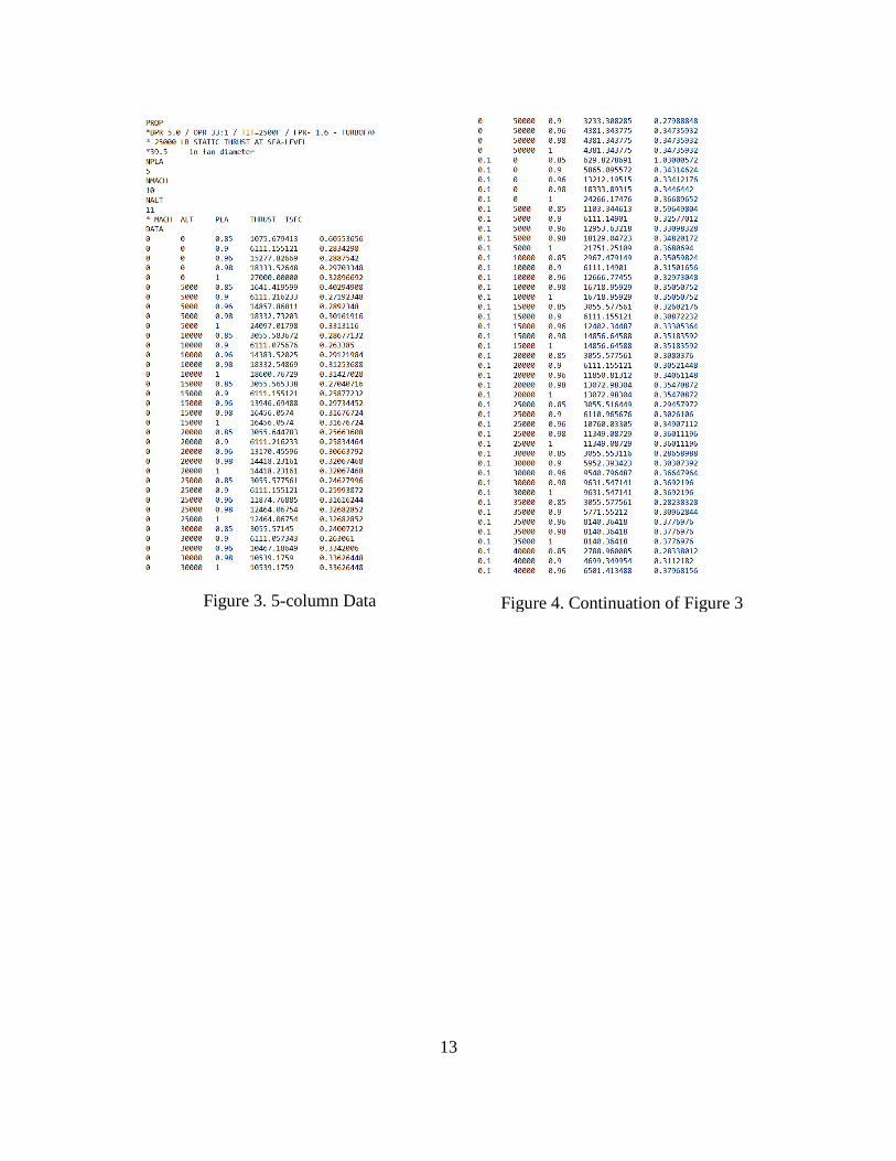
13

Figure 4. Continuation of Figure 3

Figure 3. 5-column Data

14

Chapter 3: Aerodynamic Database Generator

Figure 5 is a flowchart that shows how the overall sketch-to-VMC process

operates.

Figure 5. Flowchart of Main Algorithm

For each individual airplane, first we collect the line art and geometric

parameters, and enter these into the first sheet of the master EXCEL book (Figure 6). The

line art of the airplane is sub-divided into “panels” that are essentially glued together to

represent (in a flat panel vortex lattice model) the aerodynamics of the aircraft.

There are also key parameters that are unique to each aircraft that are also

inputted into VORLAX to generate the aircraft performance variables. These inputs

include Mach numbers, angles of attack (), Sideslip Angle (), Reference Area (Sref),

Collect Line art and

geometric parameters

Input parameters into

Master EXCEL input

sheet (Figure 6)

Generate formatted

input files

(Figure 10)

Pass input files

through VORLAX Import VORLAX

outputs into EXCEL

(Figure 11)

Calculate stability

derivatives

(Figure 12)

Calculate VMCG

(Figure 14)

Calculate VMCA

(Figure 16)

Post process data into

graphs and trends

15

Reference Chord (CBAR), Longitudinal Center of Gravity (XBAR), Vertical Center of

Gravity (ZBAR), and Reference Span (WSPAN).

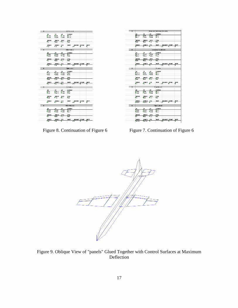
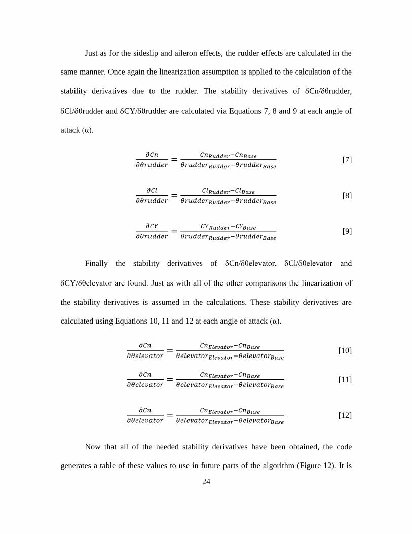
For example, with a C130J-30 there are 14 panels that constitute the line art of the

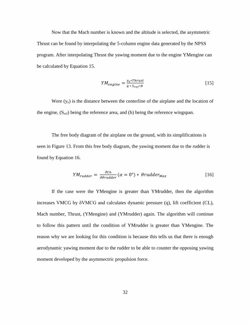
aircraft (Figure 6, Figure 8 and Figure 7). For the panels that represent the control

surfaces such as the ailerons, elevators, and the rudder, the panels are defined with the

maximum angle of deflection respectively. The final view of the aircraft would be one

were the rudder, elevators, and ailerons are at full deflected, as well as any flap panels for

the specified flaps setting (Figure 9).

Once the inputs and geometric parameters are accurate and match the desired

airplane design and shape, the VBA code then generates five different input files to be

passed into VORLAX. VORLAX is an application that is coded in FORTRAN, therefore

the input files must be very specific on spacing as well as where text may and may not

be. Figure 10 is an example of what the input file must look like. Figure 10 is only a

small portion of what the entire input file looks like, for the entire input file includes all

of the panels that were defined in the master EXCEL input sheet (Figure 6 and Figure 7).

In order to generate these very specific input files, there was a lot of coding done

to ensure spacing and location of all of the values and text of the input files. The intent of

running VORLAX is to be able to get a baseline of how the airplane flies as well as how

the control surfaces affect this baseline.

16

As mentioned earlier there will be five different input files that are generated to be passed

through VORLAX. The five different files will be referred to as Baseline, Sideslip,

Aileron, Rudder and Elevator. These five files will be discussed in deeper detail below.

Figure 6. Master EXCEL Input Example Using C130J-30 Inputs

17

Figure 9. Oblique View of "panels" Glued Together with Control Surfaces at Maximum

Deflection



18

The first input file generated represents the longitudinal Baseline aerodynamic

properties. This is the case where the aircraft flies at zero sideslip angle and all control

surface deflections are set to neutral (zero). This is done by overriding whatever the

sideslip angle () is in the master EXCEL input sheet to zero degrees. Then the code

finds the panels that represent the ailerons, rudder and elevators and manually straightens

them to a deflection of zero degrees (AINC=0). This input file is generated with the title

of Baseline, meaning it is just the baseline of aircraft performance parameters of the

aircraft. Although there is no sideslip angle or deflection of the control surfaces, the flaps

are still represented as extended and deflected to the appropriate flaps setting. The intent

of this first VORLAX input file is to generate performance parameters of the airplane in

takeoff flaps settings, thus the flaps still need to be represented in the baseline outputs to

paint a clear picture of how the airplane behaves in this flight configuration. From this

run, we compute CL vs , Cm vs and CD vs .

Figure 10. Formatted Input File for VORLAX Using C130J-30 Inputs

19

The second input file generated by the VBA code is the Sideslip case. Then intent

of this VORLAX input file is to be able to compare the outputs with the Baseline

configuration to see how sideslip winds affect the airplanes performance; it provides the

basis to develop linearized dependent aerodynamic derivatives. This input file has a

forces the sideslip angle to one degrees, however all three of the control surface need to

remain at zero degrees of deflections. Thus, like in the Baseline configuration, the code

forces the deflection angle of the ailerons, rudder and elevators to zero degrees. From this

run, we compute CY/ vs , Cn/ vs and Cl/vs .

Now that the Baseline and Sideslip input files have been generated, we need to

see how the control surfaces affect the airplane, thus the third input file that is generated

has the intent on isolating the effects of the ailerons on the airplane performance. The

third input file, titled Aileron, is generated the same way as the first two via the code that

generates these VORLAX input files. The sideslip angle is forced to zero degrees, same

as the Baseline configuration, the rudder and elevator panels are also forced to zero

degrees of deflection, however whatever is inputted in the master EXCEL input sheet as

the maximum angle of deflection for the aileron panels will be the angle of deflection for

the ailerons in this input file. From this run, we compute CY/θaileron vs ,

Cn/θaileron vs and Cl/θdaileronvs .

The fourth input file is titled Rudder, with the intentions of isolating the rudder

effects on the airplane performance parameters. Just as in the Baseline and Aileron

configurations, the sideslip angle is forced to zero degrees. The aileron and elevator

20

panels are also found via the search algorithm and set to zero degrees deflection. When

the rudder panel is isolated and generated in the input file, the angle of deflection that is

inputted in the master EXCEL sheet is what will be generated in the VORLAX input file.

From this run, we compute CY/θrudder vs , Cn/θrudder vs and Cl/θruddervs

.

The fifth and final VORLAX input file that is generated is the one intended on

isolating the effects of the elevator on the airplane. Thus this final file, titled Elevator,

has a sideslip angle of zero degrees. The aileron and rudder panels are forced to a

deflection of zero degrees, and the elevator panels are generated exactly as they are

defined in the master EXCEL sheet, thus representing an airplane that has only the

elevators that are influencing the performance parameters of the airplane. From this run,

we compute CL/θelevator vs , CD/θelevator vs and Cm/θelevatorvs .

It is important to remember that as in the Baseline configuration, all of the other

four input files represent the airplane in takeoff flaps configuration, thus the panels that

represented the inboard and outboard flaps are extended and angled to the specified

takeoff settings. For the case of the C130J-30 takeoff flaps setting, which is represented

in all of the example figure, the angle of the flaps is eighteen degrees. For eighteen

degrees to be represented accurately, this angle must be added to any deflection angle of

the wing. For example the inboard wing has a deflection of about four degrees; therefore

the inboard flaps have a deflection of twenty-two degrees to allow the flaps to be

represented at eighteen degrees.

21

Moving on to the fourth section of Figure 5, all five of the VORLAX input files

are passed through the VORLAX program in sequence, one at a time. Each individual

execution of the VORLAX program generates an output file. This output file is called the

log file, and has more information in it than is needed to calculate VMCG and VMCA.

Due to the fact that all of this information is not needed, the code then parses this

information into another output file that is specific for the needs of calculating VMCG

and VMCA. This information includes Lift coefficient (CL), Drag coefficient (CD),

Lateral force coefficient (CY), Pitching moment coefficient (Cm) (designated CPM in the

VORLAX output file), Rolling moment coefficient (Cl) (designated CRM in the

VORLAX output file), and Yawing moment coefficient (Cn) (designated CYM in the

VORLAX output file).

Figure 11 shows exactly what information is parsed form the log file and then

imported into another EXCEL sheet. The Baseline VORLAX file was passed through

VORLAX and the values seen in Figure 11 as the parsed values needed for solving

VMCG and VMCA. As seen in Figure 11 there is only one Mach number used and

fifteen different angles of attack (α) with corresponding performance parameters of CL,

CD, CY, CPM, CRM and CYM. It is noted that there is no CY, CRM or CYM values;

this makes sense because there are not control surfaces deflected nor is there any sideslip

angle. This is a good way of gut checking the outputs of the Base file.

22

Figure 11. Imported Vorlax Output into EXCEL Using C130J-30 Inputs

The code then parses and grabs this information for the Sideslip, Aileron,

Rudder and Elevator VORLAX output files. Now that all of this information is

generated, there is a database that can be used to interpolate any information desired

within the scope of the inputs.

The next step in the process is to determine the stability derivatives in terms of

sideslip angle, aileron deflection, rudder deflection and elevator deflection. At this point

an assumption is made to be able to calculate these stability derivatives. The assumption

is that the effects of sideslip angle and the control surfaces are linear. By making this

assumption, we are able to compare the output values at every angle of attack (α) for each

performance parameter and derive the stability derivatives, then interpolate these values

when solving for VMCG and VMCA. One of the major discoveries of this work, which

will be elaborated on later, is the observation that this linearization of the stability

derivatives for each individual angle of attack (α) still produces an accurate estimation of

VMCG and VMCA.

23

For example the Sideslip configuration had a sideslip angle of one degree, if we

assume the stability derivatives of Cn/Cl/and CY/to be linear, then each of

the stability derivatives of Cn/Cl/and CY/may be calculated by Equations

1, 2 and 3 respectively at each angle of attack (α). If there is a sideslip angle of three

degrees, then the effects would just be three times these stability derivatives, due to the

linearization of these stability derivatives.

𝜕𝐶𝑛

𝜕𝛽=

𝐶𝑛𝑆𝑖𝑑𝑒𝑠𝑙𝑖𝑝−𝐶𝑛𝐵𝑎𝑠𝑒

𝛽𝑆𝑖𝑑𝑒𝑠𝑙𝑖𝑝−𝛽𝐵𝑎𝑠𝑒 [1]

𝜕𝐶𝑙

𝜕𝛽=

𝐶𝑙𝑆𝑖𝑑𝑒𝑠𝑙𝑖𝑝−𝐶𝑙𝐵𝑎𝑠𝑒


𝜕𝐶𝑌

𝜕𝛽=

𝐶𝑌𝑆𝑖𝑑𝑒𝑠𝑙𝑖𝑝−𝐶𝑌𝐵𝑎𝑠𝑒


The next step in the process is to calculate the stability derivatives due to the

aileron effects. To do this the same linearization assumption is applied to the comparison

of the Baseline and Aileron output configuration files. The stability derivatives of

Cn/θaileron, Cl/θaileron and CY/θaileron are calculated via Equations 4, 5 and 6

at each angle of attack (α).

𝜕𝐶𝑛

𝜕𝜃𝑎𝑖𝑙𝑒𝑟𝑜𝑛=

𝐶𝑛𝐴𝑖𝑙𝑒𝑟𝑜𝑛−𝐶𝑛𝐵𝑎𝑠𝑒

𝜃𝑎𝑖𝑙𝑒𝑟𝑜𝑛𝐴𝑖𝑙𝑒𝑟𝑜𝑛−𝜃𝑎𝑖𝑙𝑒𝑟𝑜𝑛𝐵𝑎𝑠𝑒 [4]

𝜕𝐶𝑙


𝐶𝑙𝐴𝑖𝑙𝑒𝑟𝑜𝑛−𝐶𝑙𝐵𝑎𝑠𝑒


𝜕𝐶𝑌


𝐶𝑌𝐴𝑖𝑙𝑒𝑟𝑜𝑛−𝐶𝑌𝐵𝑎𝑠𝑒


24

Just as for the sideslip and aileron effects, the rudder effects are calculated in the

same manner. Once again the linearization assumption is applied to the calculation of the

stability derivatives due to the rudder. The stability derivatives of Cn/θrudder,

Cl/θrudder and CY/θrudder are calculated via Equations 7, 8 and 9 at each angle of

attack (α).

𝜕𝐶𝑛

𝜕𝜃𝑟𝑢𝑑𝑑𝑒𝑟=

𝐶𝑛𝑅𝑢𝑑𝑑𝑒𝑟−𝐶𝑛𝐵𝑎𝑠𝑒

𝜃𝑟𝑢𝑑𝑑𝑒𝑟𝑅𝑢𝑑𝑑𝑒𝑟−𝜃𝑟𝑢𝑑𝑑𝑒𝑟𝐵𝑎𝑠𝑒 [7]

𝜕𝐶𝑙


𝐶𝑙𝑅𝑢𝑑𝑑𝑒𝑟−𝐶𝑙𝐵𝑎𝑠𝑒


𝜕𝐶𝑌


𝐶𝑌𝑅𝑢𝑑𝑑𝑒𝑟−𝐶𝑌𝐵𝑎𝑠𝑒


Finally the stability derivatives of Cn/θelevator, Cl/θelevator and

CY/θelevator are found. Just as with all of the other comparisons the linearization of

the stability derivatives is assumed in the calculations. These stability derivatives are

calculated using Equations 10, 11 and 12 at each angle of attack (α).

𝜕𝐶𝑛

𝜕𝜃𝑒𝑙𝑒𝑣𝑎𝑡𝑜𝑟=

𝐶𝑛𝐸𝑙𝑒𝑣𝑎𝑡𝑜𝑟−𝐶𝑛𝐵𝑎𝑠𝑒

𝜃𝑒𝑙𝑒𝑣𝑎𝑡𝑜𝑟𝐸𝑙𝑒𝑣𝑎𝑡𝑜𝑟−𝜃𝑒𝑙𝑒𝑣𝑎𝑡𝑜𝑟𝐵𝑎𝑠𝑒 [10]

𝜕𝐶𝑛




𝜕𝐶𝑛




Now that all of the needed stability derivatives have been obtained, the code

generates a table of these values to use in future parts of the algorithm (Figure 12). It is

25

important to remember that although the linearization assumption was made for the

stability derivatives, the Mach number and angle of attack (α) dependencies were not

linearized.

Each Equation 1 through 12 is solved at each angle of attack (from zero to

fourteen degrees. As seen in Figure 12, the database generated for the stability derivatives

is angle of attack (α) dependent. Just like for the Mach number, once an angle of attack

(α) is interpolated, then the stability derivative values will also be interpolated within a

single degree of angle of attack (α) to account for the non-linearity dependency of angle

of attack (α).

Figure 12. Recorded Stability Derivatives in EXCEL Using C130J-30 Inputs

This generated database has the benefit and pro of searching for and accounting

for some non-linear characteristics of aircraft aerodynamics. However, this database

linearizes all stability derivatives and therefore is not as comprehensive as what you

might obtain from an extensive wind tunnel test program. In a wind tunnel, we would test

the airplane model with a range of Mach numbers, angle of attack (α) and sideslip

including getting data at several sideslip angles simultaneously with several different

26

control surface deflections. We might isolate each control surface as max up, half up,

neutral, half down, and full down, for each control surface. However wind tunnel data in

not perfect either; it needs to be adjusted for Reynolds number effects or “crud drag”

arising from excrescences and other imperfections of the skin along the actual airplane.

Once again, the assumption of linearization of the stability derivatives due to the

control surfaces is found to be acceptable due to the interpolation and algorithm used in

finding the minimal control airspeeds. If the time was spent in writing more input files

and running them through VORLAX at different deflections of the control surfaces to

generate a deeper aerodynamics database, the final solution would not be affected

significantly for the amount of time and computing power required to do so.

Now that a comprehensive aerodynamic database is generated, we can use

numerical methods to find the flight configurations needed to satisfy the trim conditions

necessary for minimal control speeds of VMCG and VMCA. As defined earlier, trim

conditions are when the forces and moments on the airplane in powered flight are

neutralized in every axis.

At this point, all of the aerodynamic forces and moments are generated in a

database, and are ready to be used in balancing the asymmetric propulsion force. Using

the NPSS generated five-column data; the algorithm will use interpolation of the

nonlinear data between two significantly small numbers to account for the non-linearity

27

dependency of Mach number. This will then allow us to have a database of aerodynamics

and a database of propulsion data to be able to solve for VMCG and VMCA.

28

Chapter 4: Computing Minimum Control Speed on the Ground (VMCG)

Minimum control speed on the ground (VMCG) is calculated when the airplane is

still on the ground rolling on its landing gear. This knowledge simplifies the calculation

of VMCG in several different ways. First off, the lift generated by the airplane does not

have to equal or be higher than the weight of the airplane, because some fraction of the

airplanes weight is supported by the landing gear. This in conjunction with the fact that

Federal Aviation Administration (FAA) rules do not permit any credit for nose wheel

steering10

, thus the calculation of VMCG is non-dependent on weight.

Another simplification of solving for VMCG is that the aerodynamic pitching

moments and rolling moments need not to be neutralized. The landing gear supports and

counters any non-zero aerodynamic moments acting on the airplane. At the same time,

the landing gear prohibits the aircraft from rolling left-to-right. The last significant

simplification is that the angle of attack (α) of the airplane is zero degrees, due to the fact

that the airplane is still on the ground, thus meaning there is no need to interpolate

between angles of attack (α).

These simplifications mean that VMCG is found when the yawing moment due to

the control surfaces is greater or equal to the yawing moment induced by the asymmetric

propulsion force of the engine. The ailerons provide a very small amount of yawing

moment; however that small amount of yawing moment comes with a large rolling

moment. Therefore, for the purposes of balancing the yawing moments, the yawing

29

moment due to the control surfaces will be generated solely by the rudder, and hence will

refer to this moment as the yawing moment due to the rudder (YMrudder).

Figure 13. Force Balance for Simplified VMCG Computation11

Figure 13 is a free body diagram of the simplified forces and moments acting on

the airplane when calculating for VMCG. This free body diagram will later be used to

generate the equation needed to solve for the VMCG.

Figure 14 is a local flowchart of how the algorithm determines VMCG. The

algorithm solves for the VMCG values at various temperature and altitudes, so that we

may find trends and discover how an airplane behaves when an engine is inoperative.

This algorithm closely follows the logic of the code used to solve for VMCG.

30

Figure 14. Flowchart of Solving for VMCG

Import geometric parameters from EXCEL

Set Temperature to lowest setting

Set Altitude to lowest setting

Import applicable 5-column propulsion data

Set VMCG to lowest setting (initial guess)

Calculate q, Mach number and Thrust

(Equations 13-14)

Solve for YMengine and YMrudder

(Equations 15-16)

YMengine

> YMrudder

YMengine

< YMrudder

Increase

by δT

Increase

by δAlt

Increase

by

δVMCG

Record VMCG and flight conditions

Altitude < max

Altitude

Altitude = max

Altitude

Temperature =

max Temperature

Temperature <

max Temperature

Done

31

For the case of the C130J-30 there are five different 5-column engine data files

that are used at temperatures of -5°C, 5°C, 15°C, 25°C and 35°C, thus the δT referred to in

Figure 14 is equal to 10°C. This particular experiment was run from an altitude of 0 ft up

to various altitudes for comparison to real data. For computational savings, the initial

guess of VMCG was set to 50 Knots, with increments δVMCG of 1 Knot. Therefore, the

first time the algorithm calculates q, CL, Mach number, Thrust, moment due to engine

(YMengine) and yawing moment due to rudder (YMrudder) it does so at a temperature of

-5°C and an altitude of 0 ft.

The dynamic pressure (q) is the kinetic energy per unit volume of fluid, in this

case air. The dynamic pressure (q) is found by taking the guessed value of VMCG (or

VMCA) and applying Equation 13.

𝑞 = ((𝑉𝑀𝐶𝐺 𝑜𝑟 𝑉𝑀𝐶𝐴)

660.8) 2 ∗ 1481 [13]

Mach number squared times dynamic pressure (qm) is a standard variable found

in the Standard Atmospheric Table (STDATM). Therefore given altitude and

temperature, the value of qm may be looked up via the SAT; for the algorithm, there is a

1976 standard atmosphere subroutine12

developed by Prof. W.H. Mason at Virginia Tech

is used to find qm. Once the qm value is known, the Mach number (M) may be found by

Equation 14.

𝑀 = √𝑞

𝑞𝑚 [14]

32

Now that the Mach number is known and the altitude is selected, the asymmetric

Thrust can be found by interpolating the 5-column engine data generated by the NPSS

program. After interpolating Thrust the yawing moment due to the engine YMengine can

be calculated by Equation 15.

𝑌𝑀𝑒𝑛𝑔𝑖𝑛𝑒 =𝑦𝑒∗𝑇ℎ𝑟𝑢𝑠𝑡

𝑞 ∗ 𝑆𝑟𝑒𝑓∗𝑏 [15]

Were (ye) is the distance between the centerline of the airplane and the location of

the engine, (Sref) being the reference area, and (b) being the reference wingspan.

The free body diagram of the airplane on the ground, with its simplifications is

seen in Figure 13. From this free body diagram, the yawing moment due to the rudder is

found by Equation 16.

𝑌𝑀𝑟𝑢𝑑𝑑𝑒𝑟 = 𝜕𝐶𝑛

𝜕𝜃𝑟𝑢𝑑𝑑𝑒𝑟(𝛼 = 0°) ∗ 𝜃𝑟𝑢𝑑𝑑𝑒𝑟𝑀𝑎𝑥 [16]

If the case were the YMengine is greater than YMrudder, then the algorithm

increases VMCG by δVMCG and calculates dynamic pressure (q), lift coefficient (CL),

Mach number, Thrust, (YMengine) and (YMrudder) again. The algorithm will continue

to follow this pattern until the condition of YMrudder is greater than YMengine. The

reason why we are looking for this condition is because this tells us that there is enough

aerodynamic yawing moment due to the rudder to be able to counter the opposing yawing

moment developed by the asymmectric propulsion force.

33

Once this condition is met, namely the condition where YMrudder is greater to or

equal to YMengine, then the algoithm records the VMCG in the EXCEL book for post

processing purposes. Then the algorithm increases the altitude by δAlt and cycles through

until the maximum specified altitude is reached, recording the VMCG at every δAlt.

Finally the algorithm increases the temperature by δT and restarts the process at an

altitude of 0 ft. The algorithm stops after finding the VMCG at every combination of

temperature and altitude. Now that VMCG has been calculated and recorded as a function

of both temperature and altitude, the algorithm moves on to finding VMCA as a function

of temperature, altitude and weight.

34

Chapter 5: Computing Minimum Control Airspeed (VMCA)

While VMCG is found when the landing gear is in contact with the ground, thus

allowing us to make simplifications to the trim condition calculations. On the other hand

VMCA is found at the flight condition where the landing gear is fully retracted and the

airplane is 400 ft above the ground13

. The airplane must be in full trim flight even with an

engine inoperative to calculate VMCA.

In the case of VMCA the lift generated by the airplane must equal the weight of

the airplane. The rolling moment, yawing moment and side force induced by the

asymmetric propulsion thrust must be countered and balanced by the control surfaces. As

another method of countering the asymmetric propulsion force induced by the engine, the

pilot is also allowed up to five degrees of bank angle (φ) as well as increasing or

decreasing the angle of attack (α), further complicating the calculation of VMCA. This

means that there are less equations than unknowns, thus this problem will be solved using

a “guess and check” brute force algorithm, much like in VMCG but with more variables.

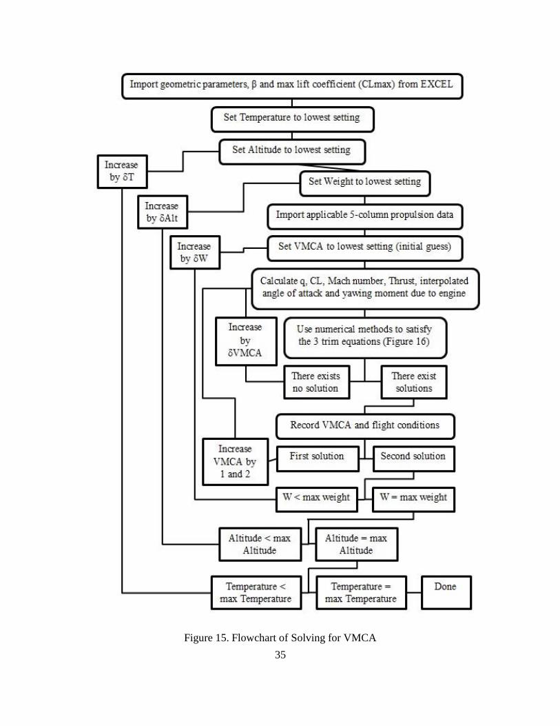
35

Figure 15. Flowchart of Solving for VMCA

36

Figure 16. Algorithm Used to Satisfy the Three Trim Equations

Import β, q, CL, Mach number, Thrust, interpolated

angle of attack (α) and yawing moment due to engine

from either VMCG or VMCA algorithm

Set δrudder to lowest value

Set δaileron to lowest value

Set bank angle φ to lowest

value

Solve for

Error1

(Equation 18)

Solve for

Error2

(Equation 19)

Solve for

Error3

(Equation 20)

Calculate Tolerance (Equation 21)

value

E > max Tolerance E < max Tolerance

add 1 φ

φ < max φ φ = max φ

add 1 δaileron

add 1 δrudder

δaileron < max δaileron δaileron = max δaileron

δrudder < max δrudder δrudder = max δrudder

Export no solution into

the algorithm of VMCG

or VMCA

Export the values of δrudder, δaileron

and φ as the flight conditions that

satisfy the trim conditions

37

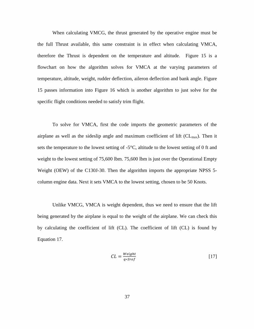
When calculating VMCG, the thrust generated by the operative engine must be

the full Thrust available, this same constraint is in effect when calculating VMCA,

therefore the Thrust is dependent on the temperature and altitude. Figure 15 is a

flowchart on how the algorithm solves for VMCA at the varying parameters of

temperature, altitude, weight, rudder deflection, aileron deflection and bank angle. Figure

15 passes information into Figure 16 which is another algorithm to just solve for the

specific flight conditions needed to satisfy trim flight.

To solve for VMCA, first the code imports the geometric parameters of the

airplane as well as the sideslip angle and maximum coefficient of lift (CLmax). Then it

sets the temperature to the lowest setting of -5°C, altitude to the lowest setting of 0 ft and

weight to the lowest setting of 75,600 lbm. 75,600 lbm is just over the Operational Empty

Weight (OEW) of the C130J-30. Then the algorithm imports the appropriate NPSS 5-

column engine data. Next it sets VMCA to the lowest setting, chosen to be 50 Knots.

Unlike VMCG, VMCA is weight dependent, thus we need to ensure that the lift

being generated by the airplane is equal to the weight of the airplane. We can check this

by calculating the coefficient of lift (CL). The coefficient of lift (CL) is found by

Equation 17.

𝐶𝐿 =𝑊𝑒𝑖𝑔ℎ𝑡

𝑞∗𝑆𝑟𝑒𝑓 [17]

38

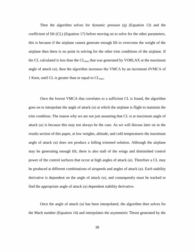
Then the algorithm solves for dynamic pressure (q) (Equation 13) and the

coefficient of lift (CL) (Equation 17) before moving on to solve for the other parameters,

this is because if the airplane cannot generate enough lift to overcome the weight of the

airplane then there is no point in solving for the other trim conditions of the airplane. If

the CL calculated is less than the CLmax that was generated by VORLAX at the maximum

angle of attack (α), then the algorithm increases the VMCA by an increment δVMCA of

1 Knot, until CL is greater than or equal to CLmax.

Once the lowest VMCA that correlates to a sufficient CL is found, the algorithm

goes on to interpolate the angle of attack (α) at which the airplane is flight to maintain the

trim condition. The reason why we are not just assuming that CL is at maximum angle of

attack (α) is because this may not always be the case. As we will discuss later on in the

results section of this paper, at low weights, altitude, and cold temperatures the maximum

angle of attack (α) does not produce a fulling trimmed solution. Although the airplane

may be generating enough lift, there is also stall of the wings and diminished control

power of the control surfaces that occur at high angles of attack (α). Therefore a CL may

be produced at different combinations of airspeeds and angles of attack (α). Each stability

derivative is dependent on the angle of attack (α), and consequently must be tracked to

find the appropriate angle of attack (α) dependent stability derivative.

Once the angle of attack (α) has been interpolated, the algorithm then solves for

the Mach number (Equation 14) and interpolates the asymmetric Thrust generated by the

39

counter operative engine. Just like VMCG, the algorithm also calculates the YMengine

using Equation 15.

Now that all of these parameters for this specific guess of VMCA have been

calculated or interpolated, the algorithm passes this information into Figure 16 to

numerically solve for any flight conditions that will satisfy the three trim equations,

namely Equations 18, 19 and 20.

In order for the airplane to be trimmed it must counter and balance the

asymmetric force produced by the engine. There are three trim equations that are

developed to satisfy the condition of balancing forces and moments that are represented

in the free body diagrams (Figure 17, Figure 18 and Figure 19).

Figure 17. Force and Yawing Moment Balance for Calculating VMCA14

40

Figure 18. Side Force Balance for Calculating VMCA14

Figure 19. Rolling Moment Balance for Calculating VMCA14

Looking at the free body diagram represented in Figure 17, the equation

developed to balance the yawning moments is seen in Equation 18.

𝐸𝑟𝑟𝑜𝑟1 = 𝜕𝐶𝑛

𝜕𝛽(𝛼) ∗ 𝛽 +

𝜕𝐶𝑛

𝜕𝜃𝑟𝑢𝑑𝑑𝑒𝑟(𝛼) ∗ 𝜃𝑟𝑢𝑑𝑑𝑒𝑟 +

𝜕𝐶𝑛

𝜕𝜃𝑎𝑖𝑙𝑒𝑟𝑜𝑛(𝛼) ∗ 𝜃𝑎𝑖𝑙𝑒𝑟𝑜𝑛 − 𝑌𝑀𝑒𝑛𝑔𝑖𝑛𝑒 [18]


developed to balance the side forces is seen in Equation 19.

𝐸𝑟𝑟𝑜𝑟2 = 𝜕𝐶𝑌

𝜕𝛽(𝛼) ∗ 𝛽 +

𝜕𝐶𝑌


𝜕𝐶𝑌

𝜕𝜃𝑎𝑖𝑙𝑒𝑟𝑜𝑛(𝛼) ∗ 𝜃𝑎𝑖𝑙𝑒𝑟𝑜𝑛 + sin(𝜑) ∗

𝑊𝑒𝑖𝑔ℎ𝑡

𝑞∗ 𝑆𝑟𝑒𝑓 [19]


developed to balance the rolling moments is seen in Equation 20.

41

𝐸𝑟𝑟𝑜𝑟3 = 𝜕𝐶𝑙

𝜕𝛽(𝛼) ∗ 𝛽 +

𝜕𝐶𝑙


𝜕𝐶𝑌

𝜕𝜃𝑎𝑖𝑙𝑒𝑟𝑜𝑛(𝛼) ∗ 𝜃𝑎𝑖𝑙𝑒𝑟𝑜𝑛 [20]

The left hand sides of all three of these equations are named Error1, Error2 and

Error3 respectively because these equations are being solved numerically, hence will

never equal exactly zero. Therefore an artificial threshold of accuracy constrains these

three trim equations. This artificial constraint is defined as the Tolerance and is

calculated by Equation 21. The airplane is considered trimmed if the Tolerance is under

the tolerance threshold of 0.0001.

𝑇𝑜𝑙𝑒𝑟𝑎𝑛𝑐𝑒 = 𝐸𝑟𝑟𝑜𝑟12 + 𝐸𝑟𝑟𝑜𝑟22 + 𝐸𝑟𝑟𝑜𝑟32 [21]

If Tolerance is greater than the threshold of 0.0001 then Figure 16 shows that “no

solution” will be passed back into Figure 15. This means that the algorithm will then

increase the guessed VMCA by an increment δVMCA of 1. Then the algorithm will

recalculate the dynamic pressure (q), coefficient of lift (CL), Mach number (M),

interpolated Thrust, interpolated angle of attack (α) and yawing moment due to the

operative engine YMengine.

After these new calculated parameters have been found, the algorithm passes

them back into Figure 16. This process of increasing the VMCA by δVMCA will

continue until there is a solution that can be found to satisfy the three trim equations

Equation 18, 19 and 20 in such a way that the Tolerance calculated in Equation 21 is

under the preset threshold of 0.0001. At the point that there is a flight configuration that

satisfies this condition, Figure 16 will pass the “there exists a solution” to the main

VMCA algorithm of Figure 15.

42

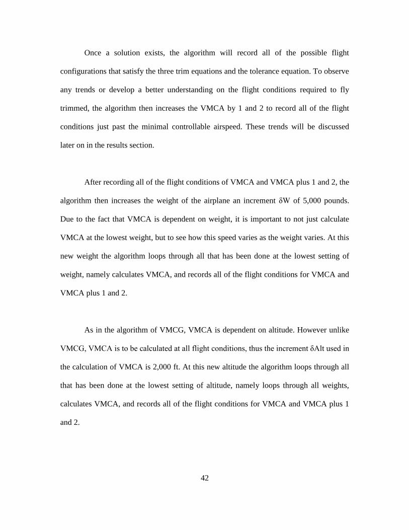
Once a solution exists, the algorithm will record all of the possible flight

configurations that satisfy the three trim equations and the tolerance equation. To observe

any trends or develop a better understanding on the flight conditions required to fly

trimmed, the algorithm then increases the VMCA by 1 and 2 to record all of the flight

conditions just past the minimal controllable airspeed. These trends will be discussed

later on in the results section.

After recording all of the flight conditions of VMCA and VMCA plus 1 and 2, the

algorithm then increases the weight of the airplane an increment δW of 5,000 pounds.

Due to the fact that VMCA is dependent on weight, it is important to not just calculate

VMCA at the lowest weight, but to see how this speed varies as the weight varies. At this

new weight the algorithm loops through all that has been done at the lowest setting of

weight, namely calculates VMCA, and records all of the flight conditions for VMCA and

VMCA plus 1 and 2.

As in the algorithm of VMCG, VMCA is dependent on altitude. However unlike

VMCG, VMCA is to be calculated at all flight conditions, thus the increment δAlt used in

the calculation of VMCA is 2,000 ft. At this new altitude the algorithm loops through all

that has been done at the lowest setting of altitude, namely loops through all weights,

calculates VMCA, and records all of the flight conditions for VMCA and VMCA plus 1

and 2.

43

The final parameter that VMCA is dependent on is the outside temperature.

Therefor after the algorithm loops through all of the different altitudes, the algorithm

increases the temperature by an increment δT of 10°C, just as it does for VMCG. At this

new temperature the algorithm loops through all that has been done at the lowest setting

of temperature. This includes looping through all the weights then altitudes to find

VMCA and records all of the flight conditions for VMCA and VMCA plus 1 and 2.

Once all of the weights, altitudes and temperatures have been looped through, and

all of the flight conditions have been recorded for VMCA and VMCA plus 1 and 2, the

post processing section can begin. This post processing section is used to calibrate the

algorithm and compare to known values of VMCG and VMCA of various airplanes. The

next section will demonstrate the accuracy of this algorithm for both the Airbus A320 and

the Super Hercules C130J-30.

44

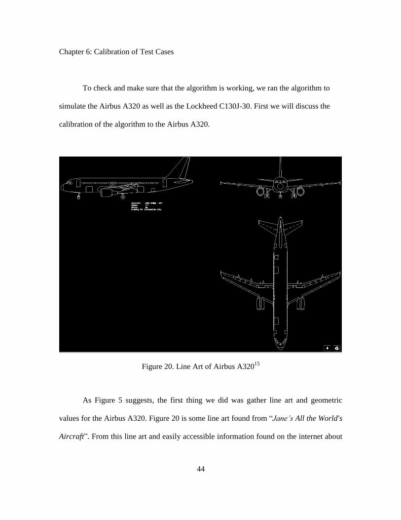
Chapter 6: Calibration of Test Cases

To check and make sure that the algorithm is working, we ran the algorithm to

simulate the Airbus A320 as well as the Lockheed C130J-30. First we will discuss the

calibration of the algorithm to the Airbus A320.

Figure 20. Line Art of Airbus A32015

As Figure 5 suggests, the first thing we did was gather line art and geometric

values for the Airbus A320. Figure 20 is some line art found from “Jane’s All the World's

Aircraft”. From this line art and easily accessible information found on the internet about

45

the A32016

, the inputs used for the Airbus A320 that were inputted into the master

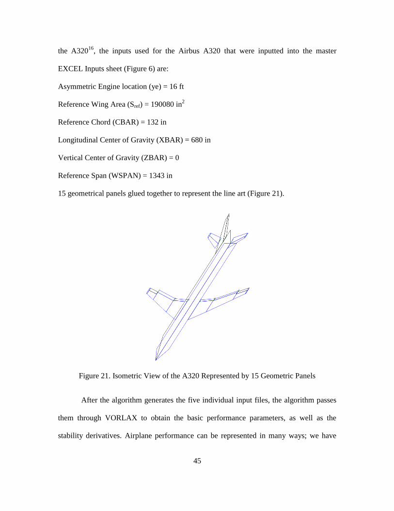
EXCEL Inputs sheet (Figure 6) are:

Asymmetric Engine location (ye) = 16 ft

Reference Wing Area (Sref) = 190080 in2

Reference Chord (CBAR) = 132 in

Longitudinal Center of Gravity (XBAR) = 680 in

Vertical Center of Gravity (ZBAR) = 0

Reference Span (WSPAN) = 1343 in

15 geometrical panels glued together to represent the line art (Figure 21).

Figure 21. Isometric View of the A320 Represented by 15 Geometric Panels

After the algorithm generates the five individual input files, the algorithm passes

them through VORLAX to obtain the basic performance parameters, as well as the

stability derivatives. Airplane performance can be represented in many ways; we have

46

chosen to represent them by three different plots, namely CL vs α (Figure 22), CD vs CL

(Figure 23) and Cm vs CL (Figure 24).

Figure 22. Coefficient of Lift (CL) Vs Angle of Attack (α) for A320 (Takeoff Flaps)

Figure 23 Coefficient of Drag (CD) Vs Coefficient of Lift (CL) for A320

(Takeoff Flaps)

47

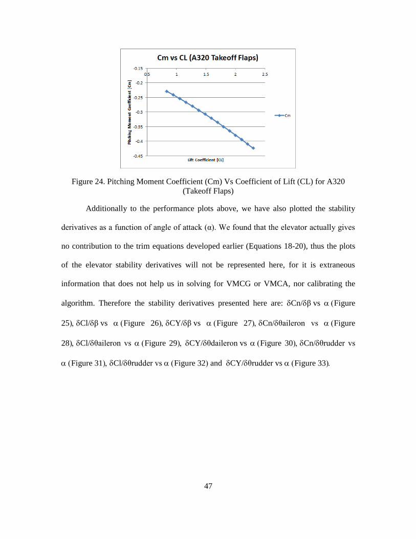
Figure 24. Pitching Moment Coefficient (Cm) Vs Coefficient of Lift (CL) for A320

(Takeoff Flaps)

Additionally to the performance plots above, we have also plotted the stability

derivatives as a function of angle of attack (α). We found that the elevator actually gives

no contribution to the trim equations developed earlier (Equations 18-20), thus the plots

of the elevator stability derivatives will not be represented here, for it is extraneous

information that does not help us in solving for VMCG or VMCA, nor calibrating the

algorithm. Therefore the stability derivatives presented here are: Cn/βvs Figure

25Cl/βvs Figure 26CY/βvs Figure 27Cn/θaileron vs Figure

28Cl/θaileron vs Figure 29 CY/θdaileronvs Figure 30Cn/θrudder vs

Figure 31Cl/θrudder vs Figure 32and CY/θruddervs Figure 33

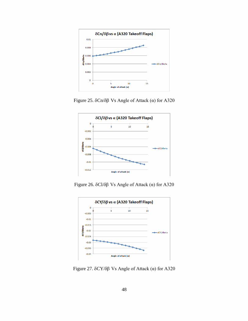
48

Figure 25. Cn/ Vs Angle of Attack (α) for A320

Figure 26. Cl/ Vs Angle of Attack (α) for A320

Figure 27. CY/ Vs Angle of Attack (α) for A320

49

Figure 28. Cn/θaileron Vs Angle of Attack (α) for A320

Figure 29. Cl/θaileron Vs Angle of Attack (α) for A320

Figure 30. CY/θaileron Vs Angle of Attack (α) for A320

50

Figure 31. Cn/θrudder Vs Angle of Attack (α) for A320

Figure 32. Cl/θrudder Vs Angle of Attack (α) for A320

Figure 33. CY/θrudder Vs Angle of Attack (α) for A320

51

According to the Airbus A320 manual, these performance parameters and

stability derivatives appear to match the actual parameters. This shows that the input files

generated and VORLAX output values are accurate enough. Therefore we can move on

to calculating and comparing VMCG and VMCA.

The Airbus manual only gives a single value for a VMCG equivalent speed

named V1, recorded at the “worst case” temperature and a range of altitudes. 14 CFR §

25.107 (a.2)17

states that V1 is calculated as VMCG plus a few extra Knots to allow the

pilot to react in time to the engine failure. As in all engineering applications that involve

human interaction, there is a delay in reaction time and action taken to correct any error.

Figure 34 is a table of the V1 values mentioned earlier. For purposed of comparison to

VMCG values calculated by the algorithm we will refer to Figure 35, a plot of

“Comparable VMCG” values vs altitude. “Comparable VMCG” values are found by

subtracting 2 Knots from the posted V1 values found in Figure 34.

52

Figure 34. Vietnam Airline A320 Performance Book Values for V2 and V118

Figure 35. Vietnam Airline A320 “Comparable VMCG” Vs Altitude of A320

53

On the other hand, we have developed an algorithm to loop through temperatures

and altitudes. Figure 36 is a plot of VMCG vs Altitude at five different temperatures;

whereas Figure 37 is a plot of VMCG vs Temperature at six different altitudes. The

values we will be comparing are the “t = ISA -20” values from Figure 36, this is because

this is the “worst case” temperature of the algorithm and the values form Figure 35 are at

the “worst case” temperature.

Figure 36. VMCG Vs Altitude at Five Different Temperatures for A320

Figure 37. VMCG Vs Temperature at Six Different Altitudes for A320

54

We can see from Figure 36 that the calculation of VMCG that we have done is

very close to the given values for the Airbus A320 at the appropriate altitude and

temperature. This means that the calibration for VMCG is verified for the Airbus A320.

Now we need to see if the VMCA portion of the algorithm can predict the flight manual

values of VMCA for the Airbus A320.

Once again the Airbus A320 manual only gives a single chart for a speed

dependent on VMCA, called V2. 14 CFR § 25.10719

states that V2 is calculated as 1.10

times VMCA. This means by looking at Figure 34 we can calculate the VMCA by

dividing the values of V2 by 1.10. Figure 38 is a plot of the VMCA values posted and

derived from the provided A320 data, whereas Figure 39 is the calculated VMCA values

fond by this algorithm.

Figure 38. VMCA Vs Weight at “Worse Case” Temperature”

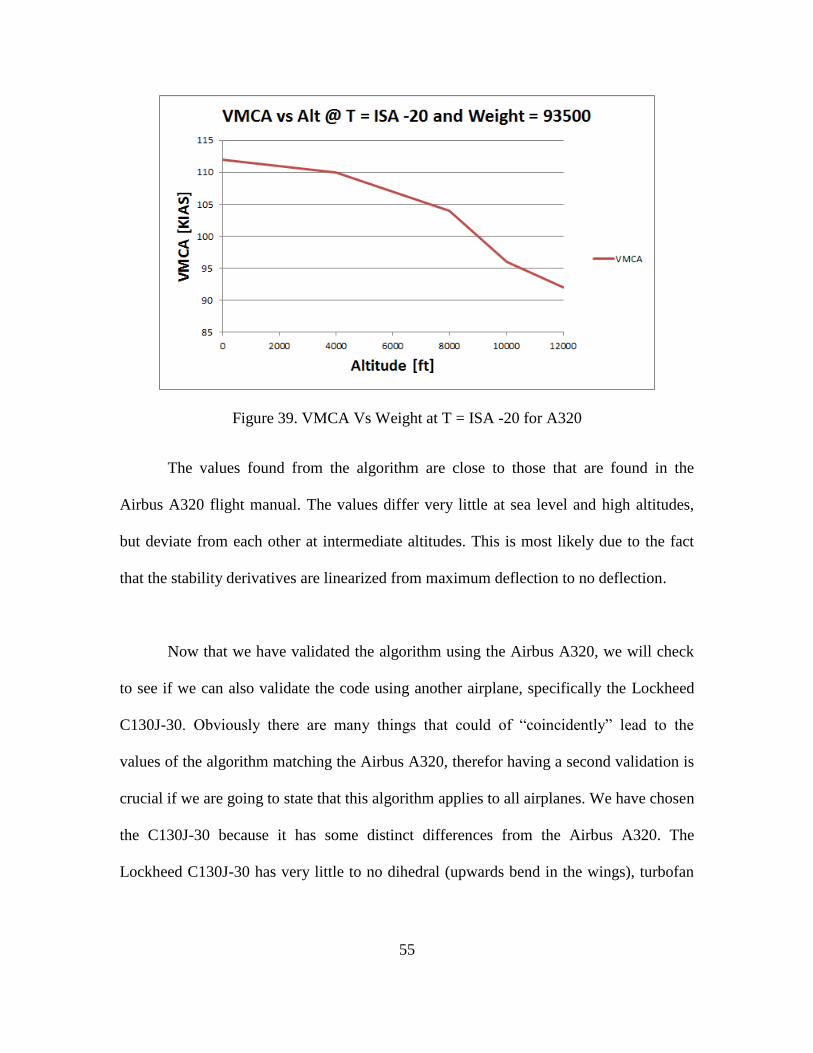
55

Figure 39. VMCA Vs Weight at T = ISA -20 for A320

The values found from the algorithm are close to those that are found in the

Airbus A320 flight manual. The values differ very little at sea level and high altitudes,

but deviate from each other at intermediate altitudes. This is most likely due to the fact

that the stability derivatives are linearized from maximum deflection to no deflection.

Now that we have validated the algorithm using the Airbus A320, we will check

to see if we can also validate the code using another airplane, specifically the Lockheed

C130J-30. Obviously there are many things that could of “coincidently” lead to the

values of the algorithm matching the Airbus A320, therefor having a second validation is

crucial if we are going to state that this algorithm applies to all airplanes. We have chosen

the C130J-30 because it has some distinct differences from the Airbus A320. The

Lockheed C130J-30 has very little to no dihedral (upwards bend in the wings), turbofan

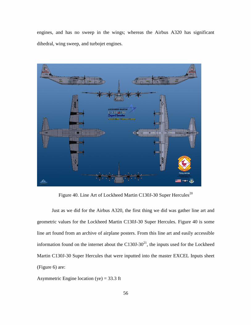
56

engines, and has no sweep in the wings; whereas the Airbus A320 has significant

dihedral, wing sweep, and turbojet engines.

Figure 40. Line Art of Lockheed Martin C130J-30 Super Hercules20

Just as we did for the Airbus A320, the first thing we did was gather line art and

geometric values for the Lockheed Martin C130J-30 Super Hercules. Figure 40 is some

line art found from an archive of airplane posters. From this line art and easily accessible

information found on the internet about the C130J-3021

, the inputs used for the Lockheed

Martin C130J-30 Super Hercules that were inputted into the master EXCEL Inputs sheet

(Figure 6) are:

Asymmetric Engine location (ye) = 33.3 ft

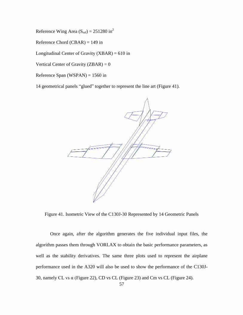
57

Reference Wing Area (Sref) = 251280 in2

Reference Chord (CBAR) = 149 in

Longitudinal Center of Gravity (XBAR) = 610 in

Vertical Center of Gravity (ZBAR) = 0

Reference Span (WSPAN) = 1560 in

14 geometrical panels “glued” together to represent the line art (Figure 41).

Figure 41. Isometric View of the C130J-30 Represented by 14 Geometric Panels

Once again, after the algorithm generates the five individual input files, the

algorithm passes them through VORLAX to obtain the basic performance parameters, as

well as the stability derivatives. The same three plots used to represent the airplane

performance used in the A320 will also be used to show the performance of the C130J-

30, namely CL vs α (Figure 22), CD vs CL (Figure 23) and Cm vs CL (Figure 24).

58

Figure 42. Coefficient of Lift (CL) Vs Angle of Attack (α) for C130J-30 (Takeoff Flaps)

Figure 43. Coefficient of Drag (CD) Vs Coefficient of Lift (CL) for C130J-30

(Takeoff Flaps)

59

Figure 44. Pitching Moment Coefficient (Cm) Vs Coefficient of Lift (CL) for C130J-30

(Takeoff Flaps)

Additionally to the performance plots above, we have also plotted the stability

derivatives as a function of angle of attack (α). Same as for the case of the A320, we

found that the elevator actually gives no contribution to the trim equations developed

earlier (Equations 18-20), thus the plots of the elevator stability derivatives will not be

represented here, for it is extraneous information that does not help us in solving for

VMCG or VMCA, nor calibrating the algorithm. Therefore the stability derivatives

presented here are: Cn/βvs Figure 45Cl/βvs Figure 46CY/βvs

Figure 47Cn/θaileron vs Figure 48Cl/θaileron vs Figure 49

CY/θdaileronvs Figure 50Cn/θrudder vs Figure 51Cl/θrudder vs

Figure 52and CY/θruddervs Figure 53

60

Figure 45. Cn/ Vs Angle of Attack (α) for C130J-30

Figure 46. Cl/ Vs Angle of Attack (α) for C130J-30

Figure 47. CY/ Vs Angle of Attack (α) for C130J-30

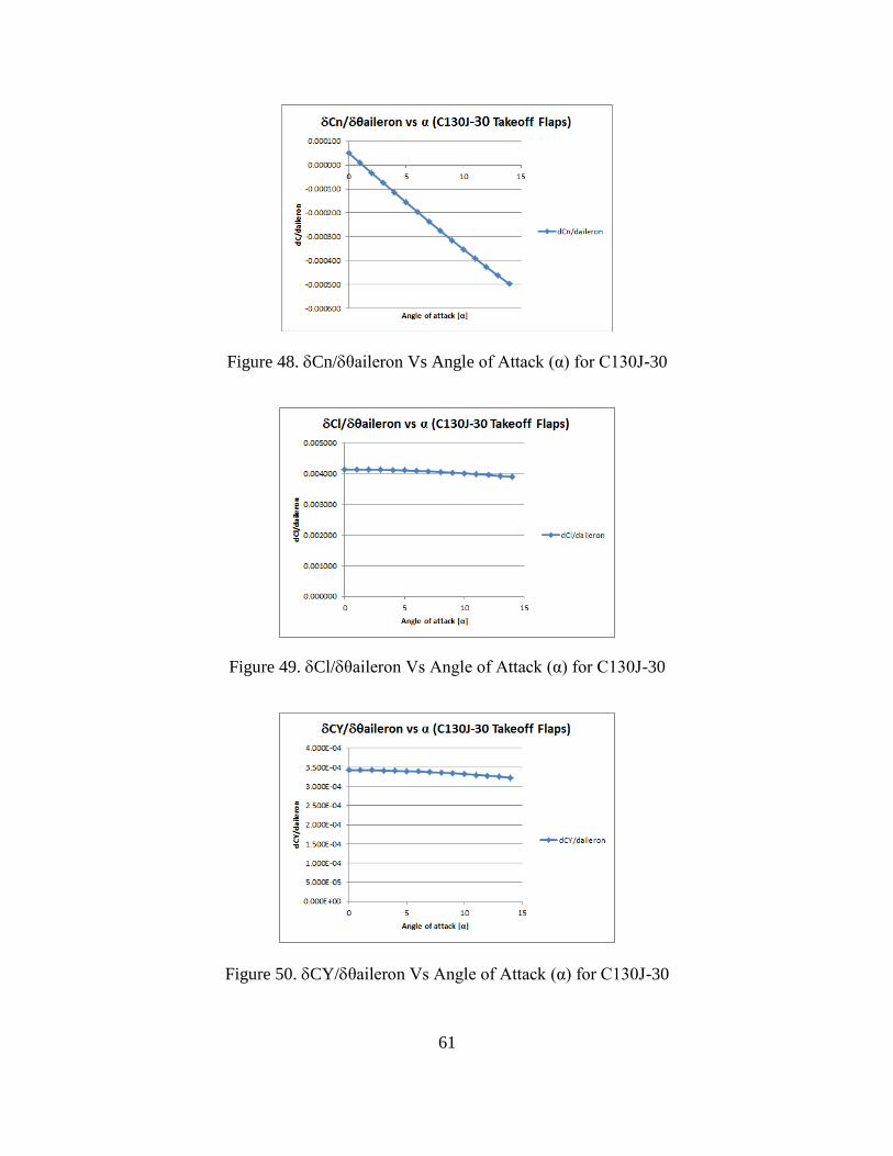
61

Figure 48. Cn/θaileron Vs Angle of Attack (α) for C130J-30

Figure 49. Cl/θaileron Vs Angle of Attack (α) for C130J-30

Figure 50. CY/θaileron Vs Angle of Attack (α) for C130J-30

62

Figure 51. Cn/θrudder Vs Angle of Attack (α) for C130J-30

Figure 52. Cl/θrudder Vs Angle of Attack (α) for C130J-30

Figure 53. CY/θrudder Vs Angle of Attack (α) for C130J-30

63

These performance parameters and stability derivatives match the actual

Lockheed Martin C130J-30 Super Hercules parameters. This shows that the input files

generated and VORLAX output values are accurate, thus allowing us to move on to

calculating and comparing VMCG and VMCA.

The C130J-30 manual only gives a multiple values of VMCG, recorded at a range

of altitudes and temperature. However, unlike the A320, the C130J-30 is used for military

transportation. This means that performance information on the C130J-30 are protected

by The International Traffic in Arms Regulations (ITAR). “ITAR is a set of United States

Government regulations on the export and import of defense related articles and

services.”22

Therefore, due to ITAR, we cannot post any official figures showing the

performance of the C130J-30, however we can state that the information we found using

this algorithm matches closely to the performance parameters of the C130J-30.

Another reason why the C130J-30 was chosen in this work is because after the

C130J-30 was manufactured and tested, it was concluded that the minimal control speeds

were much higher than desired by the military. Therefore, in order to improve the

minimal control speeds of the airplane, the engineers developed an “Automatic Thrust

Control System (ATCS) [to] optimize the balance of power on the engines, allowing

lower values of minimum control speeds and superior short-airfield performance.”23

To

create the effects of the ATCS, we decided to dial back the thrust of the engine to two-

thirds the full thrust.

64

Just as for the A320, the VMCG of the C130J-30 was found at a range of altitudes

and temperatures. Figure 54 is a plot of VMCG vs Altitude at five different

temperatures; whereas Figure 55 is a plot of VMCG vs Temperature at six different

altitudes.

Figure 54. VMCG Vs Altitude at Five Different Temperatures for C130J-30

Figure 55. VMCG Vs Temperature at Six Different Altitudes for C130J-30

65

As previously mentioned, Figure 54 and Figure 55 closely represents the values

given value for the Lockheed Martin C130J-30 Super Hercules at the appropriate altitude

and temperature. This means that the calibration for VMCG is also verified for the

C130J-30. Finally we have to verify the VMCA portion of the code, just as we did with

the A320.

The C130J-30 manual only gives a much more complicated chart for VMCA,

than that of the A320. However for the purposes of keeping the validation check

consistent, we will show a plot like the one for the A320, namely at low weight, “worst

temperature” and different altitudes. Figure 56 shows how the VMCA changes as a

function of altitude at the temperature of ISA -20°C and low weight.

Figure 56. VMCA Vs Weight at T = ISA -20 for C130J-30

The values found from the algorithm are close to those that are found in the

Lockheed Martin C130J-30 Super Hercules flight manual; therefore providing two

66

different validation cases for both VMCG and VMCA, using airplanes that are

significantly different in geometry, design and functionality.

Now that the code has been verified for the calculation of VMCG and VMCA, we

can look at patterns and trends as we discuss trade studies of simulated flight. Figure 15

shows that VMCA varies upon different parameters, it would be wise to run trade studies

with these different parameters to be able to discover and trends in minimum control

speed calculations.

67

Chapter 7: More Sophisticated Trades

In this Chapter, we will be conducting three different trade studies to show use

what is happening and this will allow us to find any patterns or discover any trends. All

of these trades that will be highlighted in this chapter will be conducted at a sideslip angle

(β) of -3°. This sideslip angle was chosen to show the reader the vast differences in

performance from one airplane to the other; implying that every individual airplane will

also likely have different effects due to sideslip angle (β).

The first trade study that we conducted is one where we held the temperature the

constant (15°C) and cycled through altitude and altitude. For the both the Airbus A320

and the Lockheed Martin C130J-30 Super Hercules, the altitude ranges from 0 to 12,000

ft in increments of 2,000 ft. The weight ranges from 93,500 lbm to 173,500 lbm in

increments of 5,000 lbm for the A320 and from 75,600 lbm to 165,600 lbm in increments

of 5,000 lbm for the C130J-30.

For this first trade we show each of the seven different altitudes in individual plots

at the International Standard Atmosphere (ISA) temperature, as well as them all together

one a single plot. We will show the information like this for the first trade study for the

purposes of completeness. For the A320 case, Figure 57 through Figure 63 is each of the

altitudes plotted in individual plots, and Figure 64 is all of them on a single plot.

68

Figure 57. VMCA Vs Weight at T = ISA and Altitude = Sea Level for A320

Figure 58. VMCA Vs Weight at T = ISA and Altitude = 2,000 Ft for A320


69




70

Figure 63 . VMCA Vs Weight at T = ISA and Altitude = 12,000 Ft for A320

Figure 64. VMCA Vs Weight at T = ISA for A320

Before we discuss and trends or observations, we will first see how VMCA

behaves for the C130J-30 airplane. This will allow us to discuss the trends between the

two airplanes, and thus come up with general statements that could be applied to any

airplane.

For the C130J-30 airplane, Figure 65 through Figure 71 is each of the altitudes

plotted in individual plots, and Figure 72 is all of them on a single plot.

71

Figure 65. VMCA Vs Weight at T = ISA and Altitude = Sea Level for C130J-30

Figure 66. VMCA Vs Weight at T = ISA and Altitude = 2,000 Ft for C130J-30


72




73


Figure 72 .VMCA Vs Weight at T = ISA for C130J-30

The first major observation that is seen is that at the maximum weight, all of the

seven different altitudes produce a VMCA that are very close to each other, suggesting

that at some point the weight of the airplane does not influence the calculation of VMCA.

This is a very interesting observation, because at the lowest weight setting it is seen for

the A320 that VMCA varies a lot. This means that there is a weight and altitude

dependent term in the calculation of VMCA that affects the calculation of VMCA at a

74

low weight, but this influence falls off when the weight reaches some point. Furthermore,

this fall off point changes as a function of altitude.

At sea level, this fall off point of the weight dependency is at a higher weight than

that of the 12,000 ft altitude scenario. For both the A320 airplane at 12,000 ft, VMCA is

a semi-straight linear line as weight increases, showing that at this altitude and weight

dependent term is purely weight dependent term, yet this trend is seen for the C130J-30

regardless of the altitude. One suggestion that would explain this observation is found by

looking at the angle of attack (α) of the VMCA solution as a function of altitude and

weight.

Figure 73. Angle of Attack (α) Vs Weight for A320

75

Figure 74. Angle of Attack (α) Vs Weight for C130J-30

Figure 73 and Figure 74 are plots of angle of attack (α) vs weight at the same

altitudes as were used in the VMCA plots of Figure 64 and Figure 72 respectively. We

observe that the fall off point that we mentioned earlier seems to coincide exactly when

the angle of attack (α) become steady and is no longer changing. Just like how VMCA

becomes dependent on weight only at 12,000 ft, the angle of attack (α) seems to linear at

this altitude for the A320. Therefore we can make the statement that at low altitudes and

weights, the limiting factor in solving for VMCA is the angle of attack (α).

If the angle of attack (α) is the limiting factor, this means that the airplane stalls

out at higher angles of attack (α); therefore VMCA is limited by stall characteristics of

the airplane. Figure 73 shows that the A320 is stall limited for a small range of altitudes

and weights. Whereas Figure 74 shows that the C130J-30 is not stall limited at any range

of altitudes and weights, most likely due to the ATCS installed.

76

On the other hand, VMCA still increases as a function of weight even after the airplane is

at its maximum angle of attack (α), thus suggesting that there is yet another limit to

VMCA that takes over once the maximum angle of attack (α) is reached. We suspect that

this other limitation is a lateral-directional control power limitation.

Earlier on we discussed the three trim equations (Equations 18-20) used to solve

for VMCA. Of these three equations, Equation 19 is the only one that is a function of

weight. Equation 19 is the equation developed to balance the side forces acting on the

airplane. The lateral-directional control power is the summation of the side forces acting

on the airplane due to the control surfaces. At higher weights, the amount of side force

needed to balance Equation 19 also increases, thus requiring higher airspeeds.

From this first trade study we have concluded that in reality VMCA is both stall

limited and lateral-directional control power limited. The 12,000 ft altitude plot could be

looked at as the underline slope of the lateral-directional control power limitation, and as

the altitude decreases, the stall limitation supersedes this underline limitation.

The next trade study we conducted was one were the weight was held constant at

a light weight, medium weight and heavy weight. Unlike for the constant temperature

trade study, we will be showing all of the altitudes on a single plot for the three different

weight configurations. This is done because it is quite fascinating what happens to

VMCA as a function of altitude and temperature when the weight increases. Figure 75 is

77

the light weight configuration, Figure 76 is the medium weight configuration and finally

Figure 77 is the heavy weight configuration for the Airbus A320.

Figure 75. VMCA Vs Temperature at Light Weight for A320

Figure 76. VMCA Vs Temperature at Medium Weight for A320

78

Figure 77. VMCA Vs Temperature at Heavy Weight for A320

Figure 78 is the light weight configuration, Figure 79 is the medium weight

configuration and finally Figure 80 is the heavy weight configuration for the Lockheed

Martin C130J-30 Super Hercules.

Figure 78. VMCA Vs Temperature at Light Weight for C130J-30

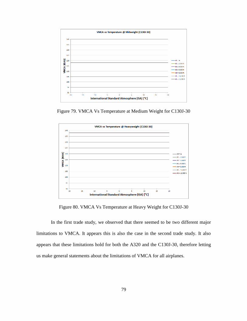
79

Figure 79. VMCA Vs Temperature at Medium Weight for C130J-30

Figure 80. VMCA Vs Temperature at Heavy Weight for C130J-30

In the first trade study, we observed that there seemed to be two different major

limitations to VMCA. It appears this is also the case in the second trade study. It also

appears that these limitations hold for both the A320 and the C130J-30, therefore letting

us make general statements about the limitations of VMCA for all airplanes.

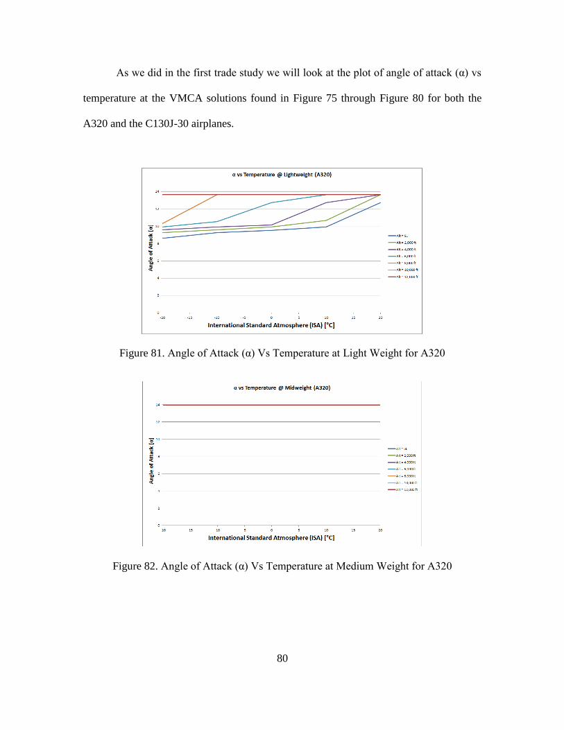
80

As we did in the first trade study we will look at the plot of angle of attack (α) vs

temperature at the VMCA solutions found in Figure 75 through Figure 80 for both the

A320 and the C130J-30 airplanes.

Figure 81. Angle of Attack (α) Vs Temperature at Light Weight for A320

Figure 82. Angle of Attack (α) Vs Temperature at Medium Weight for A320

81

Figure 83. Angle of Attack (α) Vs Temperature at Heavy Weight for A320

Figure 84. Angle of Attack (α) Vs Temperature at Light Weight for C130J-30

Figure 85. Angle of Attack (α) Vs Temperature at Medium Weight for C130J-30

82

Figure 86. Angle of Attack (α) Vs Temperature at Heavy Weight for C130J-30

Right off the bat, we notice that at medium and heavy weight the angle of attack

(α) remains constant, however at a lightweight the angle of attack (α) varies dramatically

as a function of the temperature for the A320. Just as in the first trade study, it appears

that the VMCA is stall limited at a lightweight, confirming the previous observation.

Once again we can see the effects of the ATCS on the C130J-30, for a lightweight

C130J-30 may fly at maximum angle of attack (α) thus allowing for the airplane to avoid

the unpredictability seen in the A320 case (Figure 81).

Now that we have identified one of the limitations, we will isolate the other

limitation. Looking at just the 12,000 ft altitude line we see that there is a floor, or

minimal VMCA that is calculated regardless of the temperature. The lightweight scenario

has the lowest floor VMCA and the heavy weight scenario has the highest floor VMCA,

with an intermediate floor VMCA at the medium weight scenario. This limitation is a

Thrust dependent lift limitation. In order to calculate VMCA the total amount of lift must

83

be equal to the weight of the airplane. Therefore there is a floor airspeed that the airplane

must fly at to generate enough lift to even maintain constant altitude flight.

The third trade study that was conducted was one were the altitude was held

constant at sea level, 6,000 ft and 12,000 ft and cycling through the temperature and

weight to find any trends in this last configuration.

Figure 87 is the altitude of sea level configuration, Figure 88 is the altitude of

6,000 ft configuration and finally Figure 89 is the altitude of 12,000 ft configuration for

the Airbus A320.

Figure 87. VMCA Vs Weight at Altitude of Sea Level for A320

84

Figure 88. VMCA Vs Weight at Altitude of 6,000 Ft for A320

Figure 89. VMCA Vs Weight at Altitude of 12,000 Ft for A320

Figure 90 is the altitude of sea level configuration, Figure 91 is the altitude of

6,000 ft configuration and finally Figure 92 is the altitude of 12,000 ft configuration for

the Lockheed Martin C130J-30 Super Hercules.

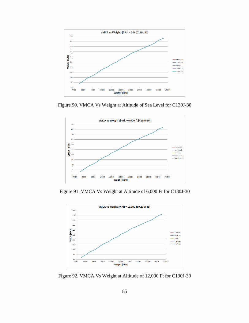
85

Figure 90. VMCA Vs Weight at Altitude of Sea Level for C130J-30

Figure 91. VMCA Vs Weight at Altitude of 6,000 Ft for C130J-30

Figure 92. VMCA Vs Weight at Altitude of 12,000 Ft for C130J-30

86

As could be predicted, there seems to be two different limitations to VMCA that

are observed in this third and final trade study. This trade study looks a lot like the first

trade study, were there seems to be some underline slope of VMCA limitation, with some

deviations at low weight, temperature, and altitude at least for the full thrust A320

airplane.

As we have for the first trade study, we will observe the angle of attack (α) as a

function of weight at the three different altitude settings for both the A320 and the

C130J-30 (Figure 93 through Figure 98).

Figure 93. Angle of Attack (α) vs Weight at Altitude of Sea Level for A320

87

Figure 94. Angle of Attack (α) Vs Weight at Altitude of 6,000 Ft for A320

Figure 95. Angle of Attack (α) Vs Weight at Altitude of 12,000 Ft for A320

Figure 96. Angle of Attack (α) Vs Weight at Altitude of Sea Level for C130J-30

88

Figure 97. Angle of Attack (α) Cs Weight at Altitude of 6,000 Ft for C130J-30

Figure 98. Angle of Attack (α) Vs Temperature at Heavy Weight for C130J-30

Once again we see that the angle of attack (α) plays a major role in calculating

VMCA. At low altitudes, the A320 airplane stalls at low weight and low temperatures

much more than in the high altitude scenario. Further confirming the statement that

VMCA is stall limited at low temperature, weight and altitude. It is important to see that

this trade study shows that there is some stall for the A320 still occurring at a medium

altitude and low temperatures, whereas at medium temperature there was no stall at

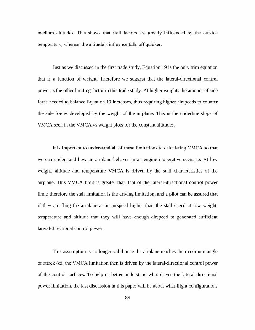
89

medium altitudes. This shows that stall factors are greatly influenced by the outside

temperature, whereas the altitude’s influence falls off quicker.

Just as we discussed in the first trade study, Equation 19 is the only trim equation

that is a function of weight. Therefore we suggest that the lateral-directional control

power is the other limiting factor in this trade study. At higher weights the amount of side

force needed to balance Equation 19 increases, thus requiring higher airspeeds to counter

the side forces developed by the weight of the airplane. This is the underline slope of

VMCA seen in the VMCA vs weight plots for the constant altitudes.

It is important to understand all of these limitations to calculating VMCA so that

we can understand how an airplane behaves in an engine inoperative scenario. At low

weight, altitude and temperature VMCA is driven by the stall characteristics of the

airplane. This VMCA limit is greater than that of the lateral-directional control power

limit; therefore the stall limitation is the driving limitation, and a pilot can be assured that

if they are fling the airplane at an airspeed higher than the stall speed at low weight,

temperature and altitude that they will have enough airspeed to generated sufficient

lateral-directional control power.

This assumption is no longer valid once the airplane reaches the maximum angle

of attack (α), the VMCA limitation then is driven by the lateral-directional control power

of the control surfaces. To help us better understand what drives the lateral-directional

power limitation, the last discussion in this paper will be about what flight configurations

90

of bank angle (φ), rudder deflection (θrudder) and aileron deflection (θaileron) satisfy the

three trim equations (Equations 18-20).

91

Chapter 8: Minimum Control Airspeed Flight Configuration Observations

The trade studies above were all conducted at a sideslip angle (β) of -3°. A

negative sideslip angle (β) means that the pilot is to “crab” into the dead engine. This

sideslip angle (β) was highlighted because it provided the most amount of discussion.

However we will say that at a positive sideslip angle (β) of say 2°, the stall limitations

that were discussed above are no longer limitations for the constant temperature and

altitude cases. This means that there is another whole database of plots and figures that

could be placed in this paper at each sideslip angle (β), however this would triple the size

of this paper and therefore congest the paper. With that being said however, we will still

discuss the general effects of sideslip angle (β) on the flight configurations of VMCA.

Starting with a constant sideslip angle (β) of -3° there are a few main observations

that can be made about the flight configurations of bank angle (φ), rudder deflection

(θrudder) and aileron deflection (θaileron). The engine that was producing the

asymmetric propulsion force is along the positive y axis, therefore a sideslip angle (β) of -

3° means that there is a cross wind that helps the rudder counter the unbalanced force.

This is a sideslip angle (β) in which there is significant stall limitations at low weight,

altitude and temperatures.

There are very many ways that we could discuss and show the flight configuration

trends, for purposes of this discussion we will be looking at a constant temperature of

15°C, while varying altitude and weight. Below are several tables that show the flight

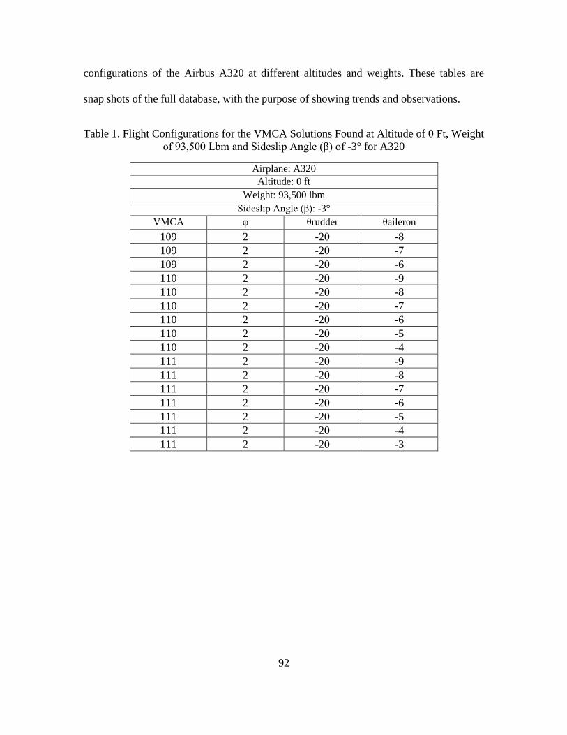
92

configurations of the Airbus A320 at different altitudes and weights. These tables are

snap shots of the full database, with the purpose of showing trends and observations.

Table 1. Flight Configurations for the VMCA Solutions Found at Altitude of 0 Ft, Weight

of 93,500 Lbm and Sideslip Angle (β) of -3° for A320

Airplane: A320

Altitude: 0 ft

Weight: 93,500 lbm

Sideslip Angle (β): -3°

VMCA φ θrudder θaileron

109 2 -20 -8

109 2 -20 -7

109 2 -20 -6

110 2 -20 -9

110 2 -20 -8

110 2 -20 -7

110 2 -20 -6

110 2 -20 -5

110 2 -20 -4

111 2 -20 -9

111 2 -20 -8

111 2 -20 -7

111 2 -20 -6

111 2 -20 -5

111 2 -20 -4

111 2 -20 -3

93



Airplane: A320

Altitude: 0 ft

Weight: 128,500 lbm



112 1 -20 -14

112 1 -20 -13

112 1 -20 -12

113 1 -20 -13

113 1 -20 -12

113 1 -20 -11

114 1 -19 -13

114 1 -19 -12

94



Airplane: A320

Altitude: 0 ft

Weight: 173,500 lbm



130 1 -19 -16

130 1 -19 -15

130 1 -19 -14

130 1 -19 -13

130 1 -19 -12

130 1 -19 -11

130 1 -19 -10

131 1 -19 -15

131 1 -19 -14

131 1 -19 -13

131 1 -19 -12

131 1 -19 -11

131 1 -19 -10

131 1 -19 -9

131 1 -18 -14

131 1 -18 -13

131 1 -18 -12

132 1 -19 -14

132 1 -19 -13

132 1 -19 -12

132 1 -19 -11

132 1 -19 -10

132 1 -19 -9

132 1 -18 -15

132 1 -18 -14

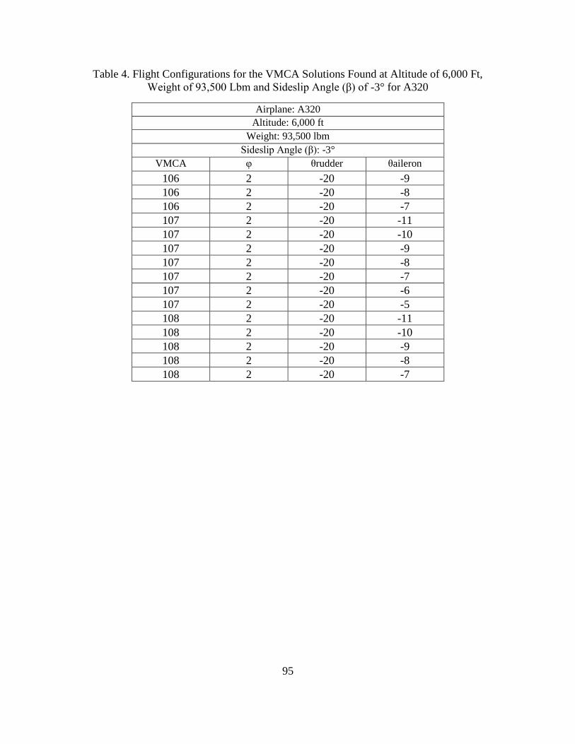
95

Table 4. Flight Configurations for the VMCA Solutions Found at Altitude of 6,000 Ft,

Weight of 93,500 Lbm and Sideslip Angle (β) of -3° for A320

Airplane: A320

Altitude: 6,000 ft

Weight: 93,500 lbm



106 2 -20 -9

106 2 -20 -8

106 2 -20 -7

107 2 -20 -11

107 2 -20 -10

107 2 -20 -9

107 2 -20 -8

107 2 -20 -7

107 2 -20 -6

107 2 -20 -5

108 2 -20 -11

108 2 -20 -10

108 2 -20 -9

108 2 -20 -8

108 2 -20 -7

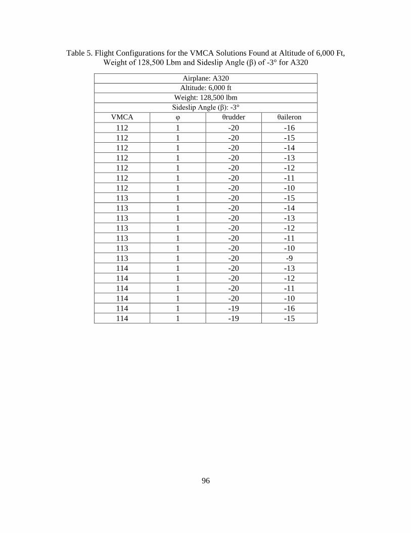
96



Airplane: A320

Altitude: 6,000 ft

Weight: 128,500 lbm



112 1 -20 -16

112 1 -20 -15

112 1 -20 -14

112 1 -20 -13

112 1 -20 -12

112 1 -20 -11

112 1 -20 -10

113 1 -20 -15

113 1 -20 -14

113 1 -20 -13

113 1 -20 -12

113 1 -20 -11

113 1 -20 -10

113 1 -20 -9

114 1 -20 -13

114 1 -20 -12

114 1 -20 -11

114 1 -20 -10

114 1 -19 -16

114 1 -19 -15

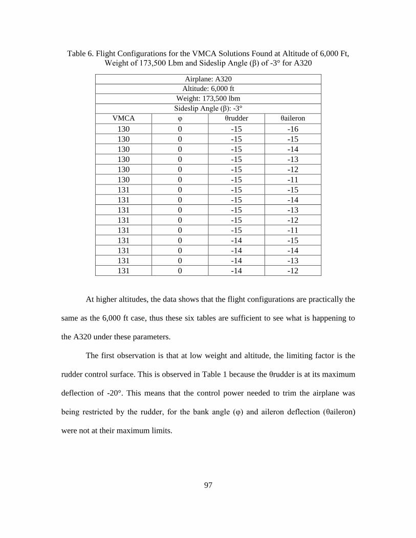
97



Airplane: A320

Altitude: 6,000 ft

Weight: 173,500 lbm



130 0 -15 -16

130 0 -15 -15

130 0 -15 -14

130 0 -15 -13

130 0 -15 -12

130 0 -15 -11

131 0 -15 -15

131 0 -15 -14

131 0 -15 -13

131 0 -15 -12

131 0 -15 -11

131 0 -14 -15

131 0 -14 -14

131 0 -14 -13

131 0 -14 -12

At higher altitudes, the data shows that the flight configurations are practically the

same as the 6,000 ft case, thus these six tables are sufficient to see what is happening to

the A320 under these parameters.

The first observation is that at low weight and altitude, the limiting factor is the

rudder control surface. This is observed in Table 1 because the θrudder is at its maximum

deflection of -20°. This means that the control power needed to trim the airplane was

being restricted by the rudder, for the bank angle (φ) and aileron deflection (θaileron)

were not at their maximum limits.

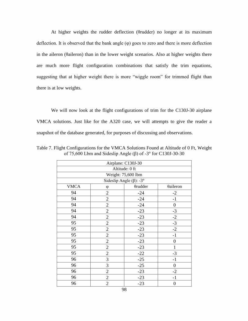
98

At higher weights the rudder deflection (θrudder) no longer at its maximum

deflection. It is observed that the bank angle (φ) goes to zero and there is more deflection

in the aileron (θaileron) than in the lower weight scenarios. Also at higher weights there

are much more flight configuration combinations that satisfy the trim equations,

suggesting that at higher weight there is more “wiggle room” for trimmed flight than

there is at low weights.

We will now look at the flight configurations of trim for the C130J-30 airplane

VMCA solutions. Just like for the A320 case, we will attempts to give the reader a

snapshot of the database generated, for purposes of discussing and observations.


of 75,600 Lbm and Sideslip Angle (β) of -3° for C130J-30-30

Airplane: C130J-30

Altitude: 0 ft

Weight: 75,600 lbm



94 2 -24 -2

94 2 -24 -1

94 2 -24 0

94 2 -23 -3

94 2 -23 -2

95 2 -23 -3

95 2 -23 -2

95 2 -23 -1

95 2 -23 0

95 2 -23 1

95 2 -22 -3

96 3 -25 -1

96 3 -25 0

96 2 -23 -2

96 2 -23 -1

96 2 -23 0

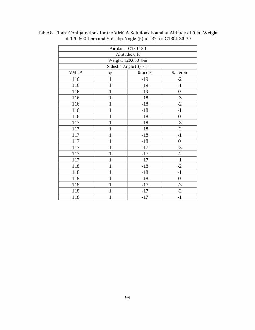
99


of 120,600 Lbm and Sideslip Angle (β) of -3° for C130J-30-30

Airplane: C130J-30

Altitude: 0 ft

Weight: 120,600 lbm



116 1 -19 -2

116 1 -19 -1

116 1 -19 0

116 1 -18 -3

116 1 -18 -2

116 1 -18 -1

116 1 -18 0

117 1 -18 -3

117 1 -18 -2

117 1 -18 -1

117 1 -18 0

117 1 -17 -3

117 1 -17 -2

117 1 -17 -1

118 1 -18 -2

118 1 -18 -1

118 1 -18 0

118 1 -17 -3

118 1 -17 -2

118 1 -17 -1

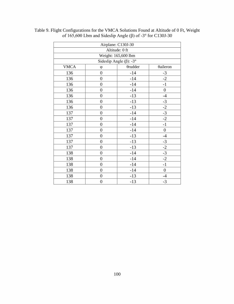
100


of 165,600 Lbm and Sideslip Angle (β) of -3° for C130J-30

Airplane: C130J-30

Altitude: 0 ft

Weight: 165,600 lbm



136 0 -14 -3

136 0 -14 -2

136 0 -14 -1

136 0 -14 0

136 0 -13 -4

136 0 -13 -3

136 0 -13 -2

137 0 -14 -3

137 0 -14 -2

137 0 -14 -1

137 0 -14 0

137 0 -13 -4

137 0 -13 -3

137 0 -13 -2

138 0 -14 -3

138 0 -14 -2

138 0 -14 -1

138 0 -14 0

138 0 -13 -4

138 0 -13 -3

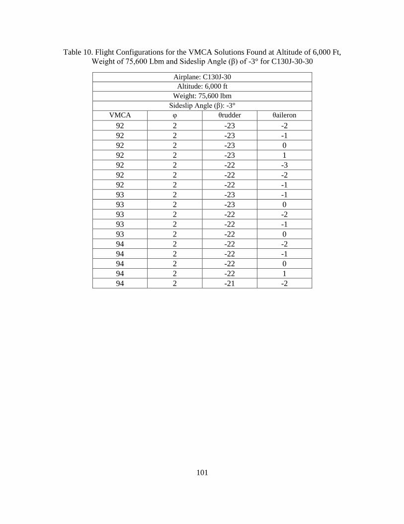
101


Weight of 75,600 Lbm and Sideslip Angle (β) of -3° for C130J-30-30

Airplane: C130J-30

Altitude: 6,000 ft

Weight: 75,600 lbm



92 2 -23 -2

92 2 -23 -1

92 2 -23 0

92 2 -23 1

92 2 -22 -3

92 2 -22 -2

92 2 -22 -1

93 2 -23 -1

93 2 -23 0

93 2 -22 -2

93 2 -22 -1

93 2 -22 0

94 2 -22 -2

94 2 -22 -1

94 2 -22 0

94 2 -22 1

94 2 -21 -2

102


Weight of 120,600 Lbm and Sideslip Angle (β) of -3° for C130J-30-30

Airplane: C130J-30

Altitude: 6,000 ft

Weight: 120,600 lbm



116 1 -18 -1

116 1 -17 -2

116 1 -17 -1

116 0 -15 -2

116 0 -15 -1

116 0 -14 -4

116 0 -14 -3

116 0 -14 -2

117 1 -18 -1

117 1 -17 -2

117 1 -17 -1

117 0 -14 -3

117 0 -14 -2

118 1 -17 -2

118 1 -17 -1

118 1 -17 0

118 0 -14 -3

118 0 -14 -2

103


Weight of 165,600 Lbm and Sideslip Angle (β) of -3° for C130J-30

Airplane: C130J-30

Altitude: 6,000 ft

Weight: 165,600 lbm



136 0 -14 -3

136 0 -14 -2

136 0 -14 -1

136 0 -14 0

136 0 -13 -3

136 0 -13 -2

137 0 -14 -2

137 0 -14 -1

137 0 -14 0

137 0 -13 -3

137 0 -13 -2

137 0 -13 -1

137 0 -13 0

137 0 -12 -3

138 0 -14 -2

138 0 -14 -1

138 0 -13 -3

138 0 -13 -2

138 0 -13 -1

138 0 -13 0

At higher altitudes, the data shows that the flight configurations are practically the

same as the 6,000 ft case, thus these six tables are sufficient to see what is happening to

the C130J-30 under these parameters.

For the C130J-30 the maximum rudder deflection is about plus or minus 25°. The

tables that show the C130J-30 flight configurations are very close to those of the A320

tables. They both are rudder control power limited, highlighted by the -25° θrudder. They

104

both are also at a small bank angle (φ) that gradually goes to zero as the weight increases.

However, a difference is the range of aileron deflection (θaileron) needed to trim the

airplane.

The fact that the rudder deflection is the same between the two airplanes shows us

that the rudder plays a significant role in trimmed engine inoperative flight. The fact that

the aileron deflections are different shows us that the trimmed flight conditions depend

on the geometry and design of the airplane. However as the weight increases, both of the

airplanes seem to go to a similar flight condition for trimmed flight.

The last step is to highlight a different sideslip angle (β) and compare the

differences between the flight configurations needed to trim the airplane. As stated

earlier, VMCA is dependent on sideslip angle (β) and there are corresponding plots to

show all of these changes, however we will just be highlighting the differences in the

flight configurations to discuss the effects of sideslip angle (β) on the trim conditions.

Just as before, the tables presented below are just snapshots of the overall

database generated by the algorithm. The purpose of the tables is to help us understand

and look for trends in flight configurations that manifest trimmed engine inoperative

flight. We will first start with the A320 airplane at a sideslip angle (β) of 2°.

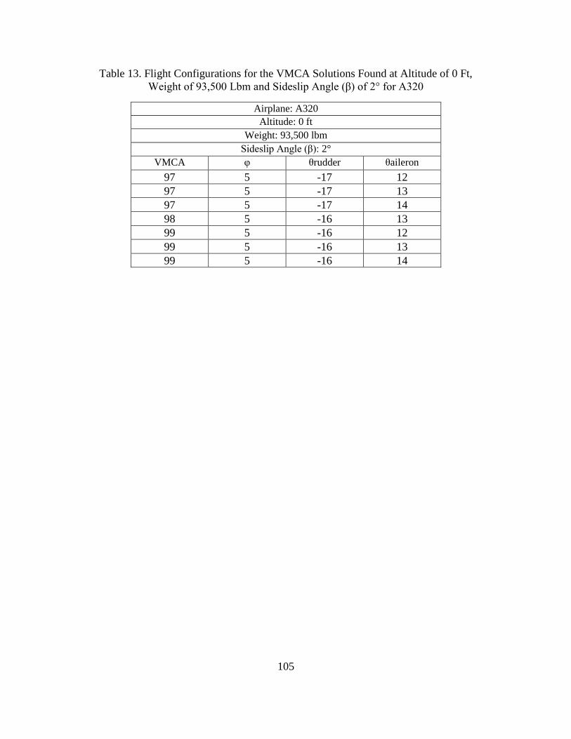
105

Table 13. Flight Configurations for the VMCA Solutions Found at Altitude of 0 Ft,

Weight of 93,500 Lbm and Sideslip Angle (β) of 2° for A320

Airplane: A320

Altitude: 0 ft

Weight: 93,500 lbm

Sideslip Angle (β): 2°


97 5 -17 12

97 5 -17 13

97 5 -17 14

98 5 -16 13

99 5 -16 12

99 5 -16 13

99 5 -16 14

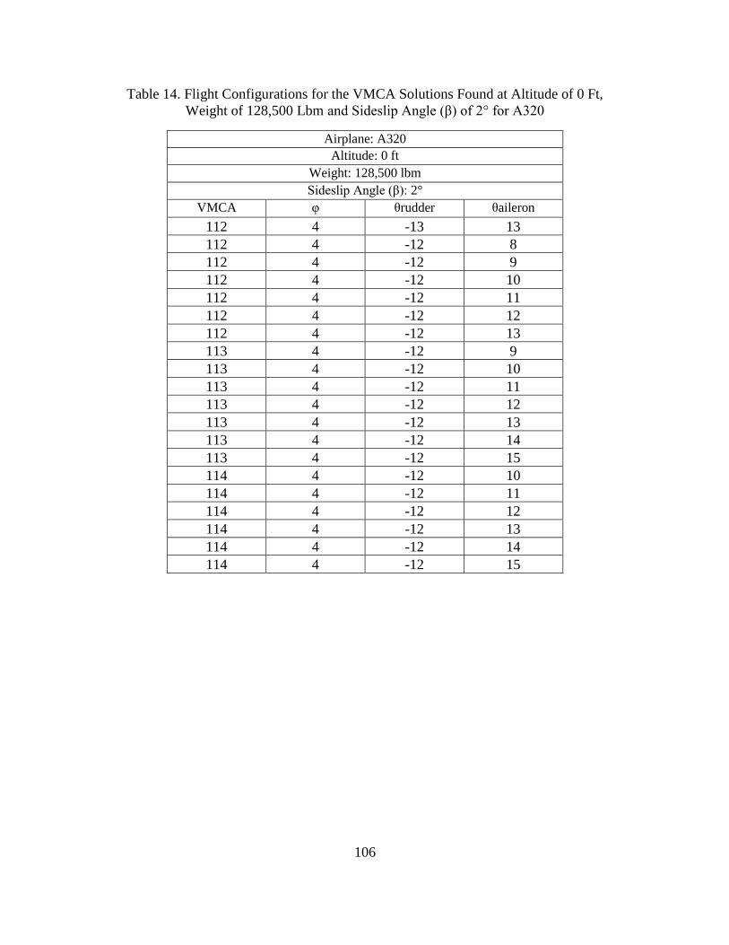
106



Airplane: A320

Altitude: 0 ft

Weight: 128,500 lbm



112 4 -13 13

112 4 -12 8

112 4 -12 9

112 4 -12 10

112 4 -12 11

112 4 -12 12

112 4 -12 13

113 4 -12 9

113 4 -12 10

113 4 -12 11

113 4 -12 12

113 4 -12 13

113 4 -12 14

113 4 -12 15

114 4 -12 10

114 4 -12 11

114 4 -12 12

114 4 -12 13

114 4 -12 14

114 4 -12 15

107



Airplane: A320

Altitude: 0 ft

Weight: 173,500 lbm



130 3 -7 8

130 3 -7 9

130 3 -7 10

130 3 -7 11

130 3 -7 12

131 3 -7 9

131 3 -7 10

131 3 -7 11

131 3 -7 12

131 3 -7 13

132 3 -7 9

132 3 -7 10

132 3 -7 11

132 3 -7 12

132 3 -7 13

132 3 -7 9

132 3 -7 10

132 3 -7 11

132 3 -7 12

132 3 -7 13

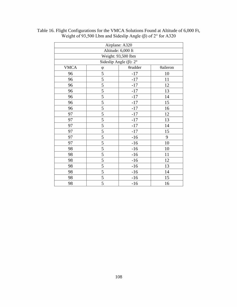
108



Airplane: A320

Altitude: 6,000 ft

Weight: 93,500 lbm



96 5 -17 10

96 5 -17 11

96 5 -17 12

96 5 -17 13

96 5 -17 14

96 5 -17 15

96 5 -17 16

97 5 -17 12

97 5 -17 13

97 5 -17 14

97 5 -17 15

97 5 -16 9

97 5 -16 10

98 5 -16 10

98 5 -16 11

98 5 -16 12

98 5 -16 13

98 5 -16 14

98 5 -16 15

98 5 -16 16

109



Airplane: A320

Altitude: 6,000 ft

Weight: 128,500 lbm



112 4 -12 10

112 4 -12 11

112 4 -12 12

112 4 -12 13

112 4 -12 14

112 4 -12 15

113 4 -12 12

113 4 -12 13

113 4 -12 14

113 4 -11 8

113 4 -11 9

113 4 -11 10

113 4 -12 12

114 4 -11 9

114 4 -11 10

114 4 -11 11

114 4 -11 12

114 4 -11 13

114 4 -11 14

110



Airplane: A320

Altitude: 6,000 ft

Weight: 173,500 lbm



130 3 -7 8

130 3 -7 9

130 3 -7 10

130 3 -7 11

130 3 -7 12

130 3 -7 13

131 3 -7 8

131 3 -7 9

131 3 -7 10

131 3 -7 11

131 3 -7 12

131 3 -7 13

132 3 -7 9

132 3 -7 10

132 3 -7 11

132 3 -7 12

132 3 -7 13

132 3 -7 14

Now that there is a positive sideslip angle (β) it seems that the rudder control

power is no longer the limiting factor in calculating VMCA. Table 13 indicated that the

bank angle (φ) is the limiting parameter. The airplane is limited to 5 degrees of bank

angle (β) per regulation, which we have previously discussed. It is also interesting to see

that the aileron deflection (θaileron) also reaches a higher deflection than in the sideslip

angle (β) of -3° case.

111

We will now compare these values to the ones for the C130J-30 at a 2° sideslip

angle (β) to see if this trend is specific to the airplane, or if it is a general trend that can be

assumed for all airplanes. The values that we get at a positive sideslip angle (β) do not

even provide a solution if the ATCS is not installed, thus further showing the need and

purpose behind the need of the ATCS for the C130J-30. However, for this work we still

applied the modified thrust in the VMCA calculations.

Table 19: Flight Configurations for the VMCA Solutions Found at Altitude of 0 Ft,

Weight of 75,600 lLbm and Sideslip Angle (β) of 2° for C130J-30

Airplane: C130J-30

Altitude: 0 ft

Weight: 75,600 lbm



92 5 -15 1

92 5 -15 2

92 5 -15 3

92 5 -15 4

93 5 -15 2

93 5 -15 3

93 5 -15 4

93 5 -14 1

94 5 -15 3

94 5 -15 4

94 5 -14 1

112


Weight of 120,600 Lbm and Sideslip Angle (β) of 2° for C130J-30

Airplane: C130J-30

Altitude: 0 ft

Weight: 120,600 lbm



116 4 -11 3

116 4 -11 4

116 4 -10 1

116 4 -10 2

116 4 -10 3

116 4 -10 4

117 4 -10 1

117 4 -10 2

117 4 -10 3

117 4 -10 4

117 4 -10 5

118 4 -10 1

118 4 -10 2

118 4 -10 3

118 4 -10 4

118 4 -9 1

118 4 -9 2

118 4 -9 3

113



Airplane: C130J-30

Altitude: 0 ft

Weight: 165,600 lbm



136 4 -9 2

136 4 -9 3

136 3 -6 1

136 3 -6 2

136 3 -6 3

136 3 -6 4

137 4 -9 2

137 4 -9 3

137 4 -9 4

137 3 -6 1

137 3 -6 2

137 3 -6 3

138 4 -9 2

138 4 -9 3

138 4 -9 4

138 4 -8 2

138 4 -8 3

138 3 -6 1

138 3 -6 2

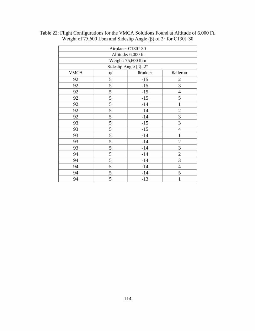
114

Table 22: Flight Configurations for the VMCA Solutions Found at Altitude of 6,000 Ft,


Airplane: C130J-30

Altitude: 6,000 ft

Weight: 75,600 lbm



92 5 -15 2

92 5 -15 3

92 5 -15 4

92 5 -15 5

92 5 -14 1

92 5 -14 2

92 5 -14 3

93 5 -15 3

93 5 -15 4

93 5 -14 1

93 5 -14 2

93 5 -14 3

94 5 -14 2

94 5 -14 3

94 5 -14 4

94 5 -14 5

94 5 -13 1

115



Airplane: C130J-30

Altitude: 6,000 ft

Weight: 120,600 lbm



116 4 -10 2

116 4 -10 3

116 4 -10 4

116 4 -9 1

116 4 -9 2

116 4 -9 3

116 4 -9 4

117 4 -10 2

117 4 -10 3

117 4 -10 4

117 4 -9 1

117 4 -9 2

117 4 -9 3

117 4 -9 4

118 4 -10 3

118 4 -10 4

118 4 -9 1

118 4 -9 2

118 4 -9 3

118 4 -9 4

118 4 -8 1

116



Airplane: C130J-30

Altitude: 6,000 ft

Weight: 165,600 lbm



136 3 -6 1

136 3 -6 2

136 3 -6 3

136 3 -6 4

136 3 -5 0

136 3 -5 1

136 3 -5 2

137 3 -6 2

137 3 -6 3

137 3 -6 4

137 3 -5 0

137 3 -5 1

137 3 -5 2

138 3 -6 2

138 3 -6 3

138 3 -5 1

138 3 -5 2

138 3 -5 3

138 3 -5 4

As mentioned for the A320, these tables show that VMCA is limited by bank

angle (φ). It is also interesting to see that in the case of the C130J-30, VMCA is also

more limited by the rudder deflection (θrudder) than aileron deflection (θaileron). Table

19 and Table 22 have values of maximum bank angle (φ) and greater values of rudder

deflection (θrudder) than aileron deflection (θaileron). This is an interesting observation,

because this is different than the A320 tables. For the case of the A320 at a 2° sideslip

angle (β), VMCA was limited by bank angle (β) and aileron deflection (θaileron).

117

Due to these observations we can state that as the sideslip angle (β) increases,

VMCA is bank angle (φ) limited as well as a control surface limited. For the A320 it is

more aileron deflection (θaileron) limited, for the C130J-30 it is more rudder deflection

(θrudder) limited at positive sideslip angles (β). Whereas both the A320 and C130J-30

share the rudder deflection (θrudder) limitation at negative sideslip angles (β). This

means that the limitations on VMCA depend on the geometry of each individual airplane.

118

Chapter 9: Conclusion

It appears that the algorithm used to calculate VMCG and VMCA produces

values that are accurate compared against published values. Although the exact values of

VMCG and VMCA for both the A320 and C130J-30 could not be found using the

algorithm, the generated values of VMCG and VMCA were close enough to show

general ideas and trends of the behavior of VMCG and VMCA.

There are many factors that go into calculating minimum control speeds, yet there

are only a few equations that are used to numerically predict VMCG and VMCA. Thus

generating a map of flight configurations needed to trim an airplane. We showed earlier

that there are some general trends like rudder deflection (θrudder) limitations at negative

sideslip angles (β), and bank angle (φ) limitations at positive sideslip angles (β). Yet we

also showed that the A320 was more aileron deflection (θaileron) limited at positive

sideslip angles (β), whereas the C130J-30 was more rudder deflection (θrudder) limited at

positive sideslip angles (β).

Each individual airplane has its own specific VMCG and VMCA characteristics

that make up its database of trimmed flight conditions. However, there may be several

types of airplanes that have the same general trends depending on dihedral, wing style,

wing sweep, length, number of engines, size of engines or other factors. Therefore with

more research there may be general categories of airplanes that would have the same

trends and limitations. This would be significant for an airliner to know which category

119

their airplanes are in to best develop and train their pilots in case of an engine inoperative

scenario.

It is crucial to have a tool developed to be able to calculate the flight

configuration options required to fly the airplane engine inoperative. There are so many

factors involved in calculating minimal control airspeeds, and it goes to show that the

current methods used are not sufficient in painting the picture on minimal control speeds.

The airplane industry is also not consistent in calculating VMCG or VMCA. The A320

manual only provided one value for VMCA depending on altitude, whereas the C130J-30

has a chart of VMCA dependent on temperature and altitude, thus increasing confusion

and inconsistency for pilots.

This work also showed that linearizing the effects of control surface deflection is

an allowable strategy when trying to calculate VMCG and VMCA. As discussed earlier

for the A320, the VMCA values calculated by the algorithm matched closely to the given

values of VMCA provided by the A320 manual at sea level and high altitudes. However,

at medium altitudes the values were less accurate. At sea level we showed that the rudder

deflection is limiting the VMCA calculations, therefore the stability derivatives used to

calculate the VMCA are the exact values found from VORLAX. However as the altitude

increases, VMCA is no longer rudder deflection limited and the stability derivatives used

to calculate VMCA are now linearized. This knowledge insinuates that if we were to

make more VORLAX files at intermediate deflections of the control surfaces, we would

most likely calculate a more accurate value of VMCA.

120

Although this work mainly focused on predicting the minimum control speeds of

existing airplanes, this algorithm could be used to aid in the design process of a new

airplane. For example, the C130J-30 has extremely high minimal control speeds without

the ATCS. This algorithm would have been able to predict this and aid the designers in

sizing the engine, rudder, aileron, elevator or wing. Due to the engine power being much

higher than needed for the geometry of the airplane, the Automatic Thrust Control

System (ATCS) was avoidably developed as a fix to overcome the poor control speeds.

The C130J-30 was able to have the ATCS because of its military use. An Automatic

Thrust Control System (ATCS) is available for use in non-military airplanes and can be

certified under 14 CFR § 25.90424

. This fact further increases the need to be able to

accurately predict minimum control speeds early on in the design of an airplane. With an

algorithm like the one described in this work, designers can run ATCS trades to evaluate

the effectiveness of using such a system. Just as with other computer aided engineering

tools, an airplane designer would be able to save a lot of time and money with the ability

to predict and calculate the minimum control speeds of an airplane using this tool.

121

REFERENCES

1 Anonymous. no date. Lockheed C130 Low-Speed Handling Qualities. Lockheed

Aeronautical Systems Co.

2 NASA. “Trimmed Aircraft”. Trimmed Aircraft. https://www.grc.nasa.gov/www/k-

12/airplane/trim.html.

3 Code770 Normals Abnormals. “Basic Aerodynamics”. Stability and Control.

http://code7700.com/stability.html.

4 14 CFR § 25.149 “Minimum control speed.” (2015)

5 Jane, Frederick, Paul Jackson. 2003. Jane’s All the World's Aircraft. London: Jane's

Information Group.

6 Haryopanji. “Lockheed Martin C-130J Super Hercules”. Deviant Art.

http://www.deviantart.com/art/Lockheed-Martin-C-130J-Super-Hercules-464814110.

7 NASA. “A Generalized Vortex Lattice Method for Subsonic and Supersonic Flow

Applications”. VORLAX.

http://ntrs.nasa.gov/archive/nasa/casi.ntrs.nasa.gov/19780008059.pdf.

8 NPSS, Numerical Propulsion System Simulation, Software Package, Ver. 2.3.0.1, Ohio

Aerospace Institute,Cleveland, OH, 2010.

9 Garnica, I., and Takahashi, T. T., “A Study of Engine Parameters and Shaft

Configuration on Transport Aircraft Performance,” AIAA 2017-#### (TBD), 2017 AIAA

SciTech Conference, January 2017.

10

Federal Aviation Administration, Flight Test Guide for Certification of Transport

Category Airplanes, Advisory Circular AC-25-7C, U.S. Department of Transportation,

Washington, D.C., Oct 16, 2012.

11

Takahashi, T.T. 2016. Aircraft Performance and Sizing: Vol II: Applied Aerodynamic

Design. New York: Momentum Press.

12

W.H. Mason. “Standard atmosphere routines”. Software for Aerodynamics and

Aircraft Design. http://www.dept.aoe.vt.edu/~mason/Mason_f/MRsoft.html#StdAtm.

13

14 CFR § 25.121 “Climb: One-engine-inoperative.” (2015)

14

Takahashi, T.T. 2016. Aircraft Performance and Sizing: Vol II: Applied Aerodynamic

Design. New York: Momentum Press.

122

15

Jane, Frederick, Paul Jackson. 2003. Jane’s All the World's Aircraft. London: Jane's

Information Group.

16

Anonymous. “Airbus A320 family”. Wikipedia.

https://en.wikipedia.org/wiki/Airbus_A320_family.

17

14 CFR § 25.107 “Takeoff speeds.” (2015)

18

Vietnam Airlines. 2008. A319/A320/A321 Flight Crew Operating Manual

19

14 CFR § 25.107 “Takeoff speeds.” (2015)

20

Haryopanji. “Lockheed Martin C-130J Super Hercules”. Deviant Art.

http://www.deviantart.com/art/Lockheed-Martin-C-130J-Super-Hercules-464814110.

21

Anonymous. “Lockheed Martin C-130J Super Hercules”. Wikipedia.

https://en.wikipedia.org/wiki/Lockheed_Martin_C-130J_Super_Hercules.

22

U.S. Department of Commerce, Bureau of Industry and Security. “EXPORT

LICENSING (ITAR & EAR)”. US Department of Commerce.

https://www.bis.doc.gov/index.php/forms-documents/doc_view/781-export-licensing.

23

Anonymous. “C-130J Hercules Tactical Transport Aircraft, United States of America”.

airforce-technology. http://www.airforce-technology.com/projects/hercules/.

24

14 CFR § 25.904 “Automatic takeoff thrust control system (ATTCS).” (2015)

Predicting Minimum Control Speed on the Ground … · 2016-12-01 · 23. Coefficient of Drag (CD)...

Documents

Transcript of Predicting Minimum Control Speed on the Ground … · 2016-12-01 · 23. Coefficient of Drag (CD)...