Predicting Hospital Readmission using TreeNet™

Robert Aronoff MD

The vision …..

Capture data entered as

part of routine clinical

workflow

EMR

Clinical Workflow

Automated E-T-L

processes

Machine learning

algorithms for target class

prediction

Predictive Model

Creation

Vendor ‘neutral’ scoring

tools:

Intranet based

JSON serialization

Decision Support

at Point of Care

Streamlined sequence of processes

Agenda / Table of contents

Readmission after Heart Failure

Data Structure of an Electronic Medical Record

TreeNet™ Modeling with our Dataset

Lessons Learned and Next Step(s)

1

2

3

4

PREFACE:

Data Modeling Paradigm

© Salford Systems, 2011

Model Accuracy

Feature Selection

Feature Fit

Target Class

Completeness of Set

Kattan MW, EuroUro. 2011; (59): 566-567

Model Error: The Bias – Variance Decomposition

Hastie T, Tibshirani R, Friedman JH. The elements of statistical learning :

Data mining, inference, and prediction. New York, NY: Springer; 2009.

Prediction Error = Irreducible Error + Bias² + Variance

Model caveats

Association does not prove causality

Models are retrospective (observational)

and therefore hypothesis generating (i.e.

not hypothesis proving)

READMISSION AFTER HEART FAILURE

Congestive Heart Failure

Common cause for admission.

Readmission in excess of 23%.

Risk factors for readmission extensively studied.

Published reviews cite over 120 studies.

- Methods: Logistic regression; Cox proportional hazard

- C-statistic in 0.6-0.7 range

Reduction of readmission has been declared a national goal.

Improved risk models have the potential to more effectively deploy

targeted disease management.

Bueno, H. et al.

JAMA 2010;303:2141-2147

EMR data structure

Data collected for clinical workflow.

Large volume

- Multiple observations; repeated measures

- Many interactions and interdependencies

Complex dataset

- Continuous, Ordinal, Nominal (low and high order), Binary

- ‘High-order variable-dimension nominal variables’

Missing data:

- May represent error or practice patterns

Unbalanced classes

Outliers and Entry errors

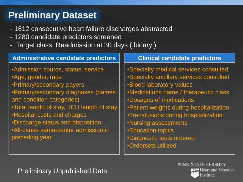
Preliminary Dataset

Administrative candidate predictors

•Admission source, status, service

•Age, gender, race

•Primary/secondary payers

•Primary/secondary diagnoses (names

and condition categories)

•Total length of stay, ICU length of stay

•Hospital costs and charges

•Discharge status and disposition

•All-cause same-center admission in

preceding year

Clinical candidate predictors

•Specialty medical services consulted

•Specialty ancillary services consulted

•Blood laboratory values

•Medications name / therapeutic class

•Dosages of medications

•Patient weights during hospitalization

•Transfusions during hospitalization

•Nursing assessments

•Education topics

•Diagnostic tests ordered

•Ordersets utilized

- 1612 consecutive heart failure discharges abstracted

- 1280 candidate predictors screened

- Target class: Readmission at 30 days ( binary )

Preliminary Unpublished Data

Benefits of Stochastic Gradient Boosting

Does not require data transformation

Handles large numbers of categorical and continuous variables

Has mechanisms for:

- Feature selection

- Managing missing values

- Assessing the relationship of predictors to target

Robust to:

- Data entry errors, Outliers, Target misclassification

Friedman JH. Stochastic gradient boosting. Computational Statistics and Data Analysis 2002; 38(4):367- 378.

Input and processing

High model accuracy

Classification and regression

Non-parametric application of logistic , L1, L2, or Huber-M loss function

Output

TreeNet™ Modeling with our Dataset

Parameters of ‘feature fit’

Parameters of ‘feature selection’

Elements of insight

Putting it all together

1

2

3

4

TreeNet – parameters of ‘feature fit’

Do not forget the manual …..

Feature selection – variable importance

Variable Importance

Calculation

Squared relative improvement

is the sum of squared

improvements (in squared

error risk) over all internal

nodes for which the variable

was chosen as the splitting

variable

Measurements are relative

and is customary to express

largest at 100 and scale other

variables appropriately

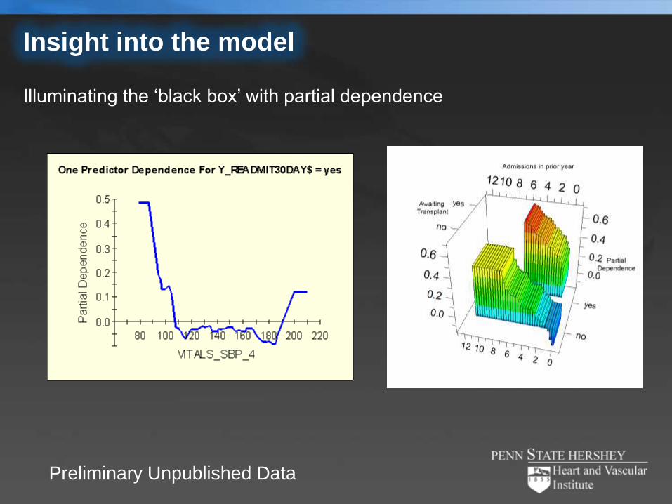
Insight into the model

Illuminating the ‘black box’ with partial dependence

Preliminary Unpublished Data

Approach to feature selection

Start with a subset

based on univariate

significance (i.e. P-

value below a given

level) or variance

above a given

threshold

Domain Neutral

Know your data

Univariate stats

Application of Variable

Importance

Screening with

batteries

Forward and backward

stepwise progression

Both

Use all potential

predictors

Use knowledge of

target and predictors to

make decisions on

inclusion (or rejection)

of predictor

Domain Centric

Domain ‘Neutral’ vs. Domain ‘Centric’

Model Variability

Variation

The model is fit via sampling (i.e.

stochastic) process.

Accuracy / Precision

S.E.M.= S.D. / sqrt ( N )

Precision (95%) ≈ 4 * S.E.M.

S.D. = 0.03

Establishing AUC precision and accuracy

N trials 10 30 300

S.E.M. .0095 .0055 .0017

Precision (95%) .038 .022 .007

Precision and predictor selection

AUC estimated using CV-10 ( = 10 trees) SEM .0095 and

precision (95%) of .038

Repeating CV-10 (using CVR battery) 30 times SEM .0017 and

precision (95%) of .007

Profound implication on dimensionality of model achievable without

domain knowledge input.

0.50

0.55

0.60

0.65

0.70

0.75

Avg

. R

OC

Test ROC

STEP_66 (737) (0.703)

Min = 0.5057

Median = 0.6738

Mean = 0.6500

Max = 0.7034

STEP_1 (197) (0.531)

How much of a change in AUC is clinically relevant ?

Gain Curve complements ROC curve

Preliminary Unpublished

Data

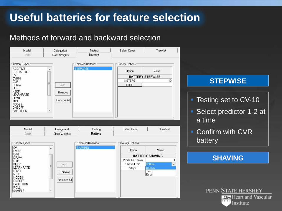
Useful batteries for feature selection

STEPWISE

SHAVING

Testing set to CV-10

Select predictor 1-2 at

a time

Confirm with CVR

battery

Methods of forward and backward selection

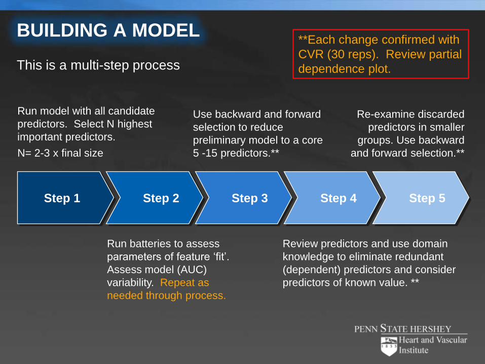
BUILDING A MODEL

Step 1 Step 2 Step 3 Step 4 Step 5

Run model with all candidate

predictors. Select N highest

important predictors.

N= 2-3 x final size

This is a multi-step process

Use backward and forward

selection to reduce

preliminary model to a core

5 -15 predictors.**

Re-examine discarded

predictors in smaller

groups. Use backward

and forward selection.**

Run batteries to assess

parameters of feature ‘fit’.

Assess model (AUC)

variability. Repeat as

needed through process.

Review predictors and use domain

knowledge to eliminate redundant

(dependent) predictors and consider

predictors of known value. **

**Each change confirmed with

CVR (30 reps). Review partial

dependence plot.

Initial runs

6 Nodes

2 Nodes

Information content and irreducible error

0.0

0.1

0.2

0.3

0.4

0.5

0.6

0 100 200 300 400 500 600 700 800 900 1000 1100 1200 1300 1400 1500

Cro

ss E

ntr

op

y

Number of Trees

Train

Test

0.576

0.577

#880 (0.518) #880 (0.518) (0.457)

0.0

0.1

0.2

0.3

0.4

0.5

0.6

0 100 200 300 400 500 600 700 800 900 1000 1100 1200 1300 1400 1500

Cro

ss E

ntr

op

y

Number of Trees

Train

Test

0.576

0.576

#287 (0.519) #287 (0.519) (0.436)

Preliminary Unpublished Data

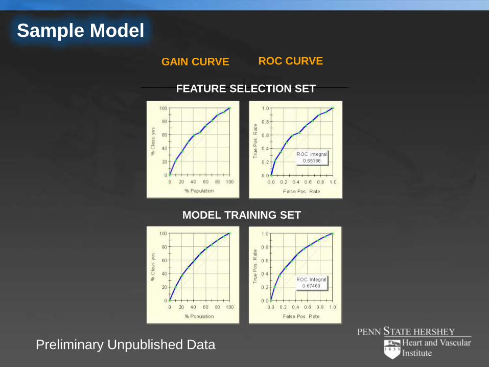
Sample Model

GAIN CURVE ROC CURVE

FEATURE SELECTION SET

MODEL TRAINING SET

Preliminary Unpublished Data

Sample partial dependence plots

The value of non-parametric regression

Admissions within prior year ICU Days

Anion Gap Initial Systolic BP

Final BNP BUN-Creatinine Ratio

Preliminary Unpublished Data

Prospective application

Additional heart failure discharges can be scored against the model

GAIN curve ROC curve

Causes for performance shift

Overfitting in the original model

Concomitant intervention programs are altering

patient risk of readmission

Preliminary Unpublished

Data

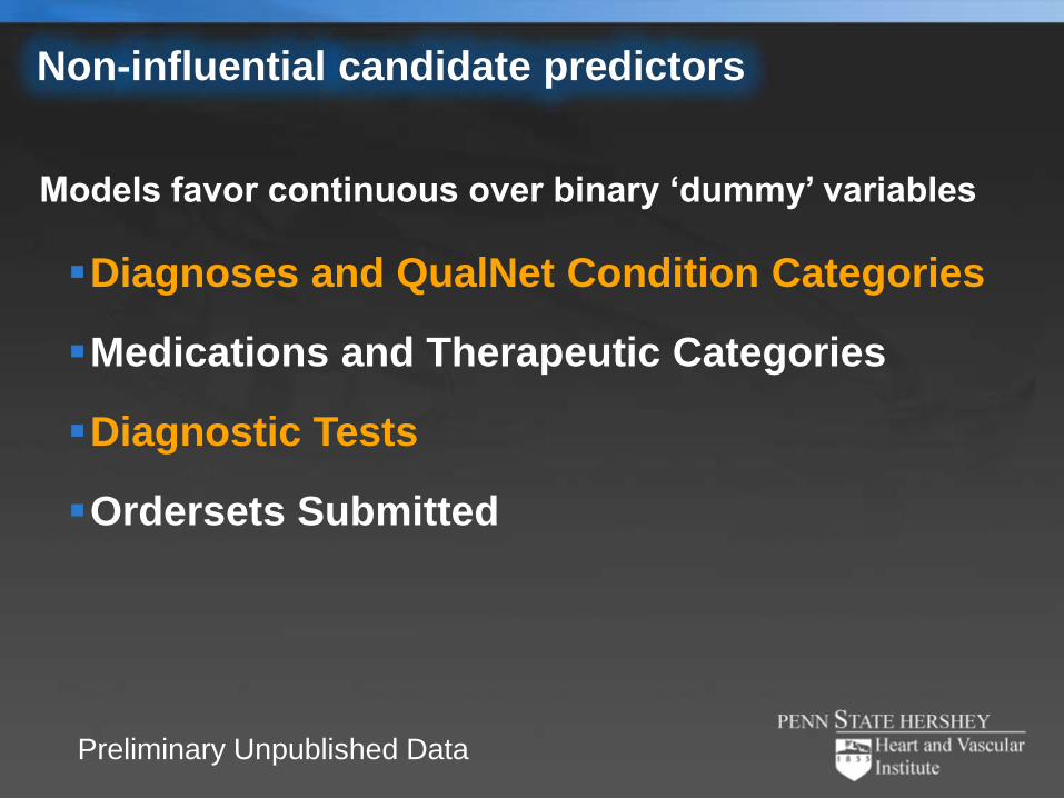
Non-influential candidate predictors

Diagnoses and QualNet Condition Categories

Medications and Therapeutic Categories

Diagnostic Tests

Ordersets Submitted

Models favor continuous over binary ‘dummy’ variables

Preliminary Unpublished Data

Lessons learned

TreeNet ( stochastic gradient boosting) is extremely well suited to

data structure of EMR data.

Insight in to dataset is a rich feature (in and above prediction

performance).

Model performance variance is important in feature selection.

- Consequence of limited information content in our dataset.

Batteries are useful.

- PARTITION – Variability assessment

- CVR – Model assessment

- STEPWISE – Forward selection

- SHAVING – Backward selection

There is great value in learning on a non-trivial dataset within a

familiar domain.

Next steps ……

Explore options to manage model variability

and increase dimensionality of predictor set.

Extend analysis of predictor interactions.

Develop mechanism of ‘point-of-care’ patient

scoring.

Apply techniques to new problems and

dataset.

Any Questions?

raronoff@hmc.psu.edu