Predicting Customers Issues Resolution Times in Mobile ... · PDF filePredicting Customers...

International Journal of Computer and Information Technology (ISSN: 2279 – 0764) Volume 02– Issue 03, May 2013

www.ijcit.com

417

Predicting Customers Issues Resolution Times in Mobile Terminals

Andi Mwegerano*

Operations, Customer Care, DfC Nokia Corporation,

Salo, Finland *andi.mwegerano{at}nokia.com

Tero Ollikainen Operations, Continuous Improvement, Lean Six Sigma

Nokia Corporation, Salo, Finland

Abstract—A factor affecting the customer satisfaction for users of a mobile terminal (MT) is how fast their possible service issues are resolved from the time they report them. As MT subscriptions have grown tremendously since the mid-eighties, the number of issues concerning the MT has grown as well. These are due to changes in factors such as technologies, applications, usability, and user interfaces. Technology changes have led to various issues that have to be resolved correctly and within a reasonable time, to keep subscribers satisfied and loyal. This paper has attempted to build a statistical model that can predict customer issue resolution times (iRT) from the moment they are reported through an inbuilt-tool for gathering Nokia product information and end user support (GENIUS). A two year (2010–2011) data bank of resolved technical issues was used to build a model to predict iRT. An initial result shows that the variable predictors selected for building the iRT model explains only 4.4% of the response variations in the model. In practice this model cannot be used in the real world and this advocates for further reaseach in the future.

Keywords- Predicting Model, Customer Satisfaction, issue resolution time

I. INTRODUCTION

The aftermarket technical support engineers in mobile terminals are often asked to estimate or predict (forecast) the amount of time needed to resolve customers’ issues from the field to keep the customer informed about their mobile phone handset. In a situation that the customer has already faced disappointment with the product, a low iRT is one of the factors that may attract customers and keep them satisfied and loyal to a company. A practical model of predicting the iRT would thus have a significant practical implication.

A. Prediction models

Prediction is the model used in this study.1

1 The terms “prediction” and “forecast” are two different words

Predicting is about saying what happens, but it may be for the past, present and future. e.g. the model predicts that an extra year of education gives 1000 euros more of income. Prediction is the process of estimating values of dependent variables based on the knowledge of an independent variable. A review by Lewis-Beck [1] clarifies the fine difference between these two words: “Forecasting aims to tell of events before they happen. It differs from

Although a prediction model would be useful, initial literature searches revealed that there is little work in mobile terminals (MT) that has attempted to predict how long a newly escalated customer issue will take to resolve. Predicting customer’s iRT is an essential part of any business activity. However predicting iRT requires setting objectives one of which is to set iRT targets. Predicting techniques vary in complexity and data requirements. However each technique fits a situation and thus an appropriate method should be used for the appropriate situation to achieve high accuracy [2]. There are many forecasting techniques, [3], one could choose from. They are: (1) Subjective (2) Time Series Techniques and (3) Cross Section Techniques. The choice of the method depends upon the nature of the data and the objective of the forecaster [2]. In extreme cases many techniques, have to be combined to achieve the objective of the project. Some researchers, in [4], [5], and [6] suggest aggregating the forecast of several methods rather than a single method. The researchers concluded that the accuracy of combined forecasts depends on both the method being used and the number of methods. They further concluded that the larger the number of methods in aggregate increases the accuracy. This argument has support [7] as it claimed that combining two different methods can frequently improve forecasting. However, combining the forecasts from different methods cannot be better than the “true” underlying model of the process generating data [8]. Regardless of the method used, if the statistical rules of the technique are not adhered to, the results will be misleading.

B. Customer satisfaction in service incidents

Service failure is one “pushing determinate” that drives customer switching behavior [9] and successful recovery can mean the difference between customer retention and defection. Companies often take too long to respond to unhappy customers, and then respond impersonally. By responding quickly, a firm conveys a sense of urgency. Quick response demonstrates that the customer's concern is the company's concern. By responding personally, with a telephone call or a

prediction in that it looks to the future, whereas prediction may not (as in a successful reconstruction of some past outcome). Further, forecasting differs from explanation, having the goal of predicting an outcome, rather than the goal of theorizing about outcomes”.


www.ijcit.com

418

visit, the firm creates an opportunity for dialogue with the customer—an opportunity to listen, ask questions, explain, apologize, and provide an appropriate remedy [10]. Speed of the response is crucial to customers [11]. Service employees need specific training to deal with dissatisfied customers and how to help customers solve a service issue. Customers judge the responsiveness, assurance, empathy and tangibles during the service delivery process; hence, these are seen as the process dimensions of the service delivery [10]. Customer satisfaction was found to be lower after service failure, even given high-recovery performance, than in the case of error-free service [12]. Research has shown that effectively handling customer complaints has a dramatic impact on customer retention and loyalty [13]. Collecting customer complaint data is common practice in many companies and has received vast research attention. Research has focused on the process to handle complaints on the customer experience and analysis of complaint data and the relationships to important business outcome [14], [15]; [16], [17], [18], [19], [20]. This paper is trying to develop a model that predicts the iRT for providing iCA i.e., service recovery for customers’ issues. The prediction model is directed towards being a practical tool for managers in after-sales process, providing both a tool for managing after-sales service and being a prediction tool aiding customer work.

The remainder of this paper is organized as follows: In section 2, we explain how and where the data was gathered and the descriptive statistics of the data is also displayed. We explain how the customer issues are escalated and the predicting model block diagram is provided with explanation. Section 3 explains the statistical procedure method. Section 4, the predicting model results and testing are tabulated and explained. In section 5, a discussion and conclusion are provided.

II. CASE AND DATA GATHERING

Nokia is one of the biggest mobile phones manufacturers in the world. Millions of phones are sold by the company. The authorized service vendors (ASV) provide services for Nokia products. The customers in this paper are the ASV’s who are in turn in contact with end users or consumers. It is important for the ASV to have an estimate of time for when a customer issue will be resolved. By knowing the iRT the ASV can for example, decide to give a loan or swap the MT to keep the customer satisfied. A two year (2010-2011) data bank of resolved technical issues is gathered and analyzed using suitable statistical methods to predict the iRT for service recovery. The following describes the after sales service issue escalation chain [21] and data gathered from the process.

A. High level customer issue escalation process

The customer issue escalation process is shown in Figure 1 below where:

SL Service Level

SL1 Authorized Service Vendor (ASV)

SL2 Country Sales Area - Care (CSAC)

SL3 Region Sales Area - Care (RSAC)

SL4 Care Product Mangers (CPM)

SL5 Product Designers (R&D)

Figure 1. SIPOC diagram of the customer issues escalation

The main suppliers in the SIPOC (Supplier, Input, Process, Output, and Customer) diagram are the mobile terminals authorized service vendors (ASV), and less frequently is the manufacturer using the country sales area technical support engineers (CSAC) and the manufacturers region sales technical support engineers (RSAC). The inputs are the customers’ issues raised by the ASV (called SL1 in the service chain network) including the product specifications like software, variant software, product samples, issue symptoms (TA), business impact (iBI) due to the issue etc. The process is described as follows: When a customer X approaches an ASV with an issue Y with his/her mobile terminal (MT), the ASV tries to find a solution for the Y issue and resolve the issue and gives back the MT to the customer X. However if the issue Y can’t be resolved by the AVS, the issue is documented into an in-house tool called GENIUS and escalated to the sales area (SA) technical support (referred as SL2 in the service chain), who then resolves the issue and returns it back to SL1 or otherwise they escalate the issue to regional sales area technical support engineers (RSAC) i.e. SL3. The process goes as described before until the issue resolution is found. The issue correction action (iCA) is the output in the SIPOC chain. The customers are mainly the ASV and indirectly the consumers i.e. end users of the MT.

B. Data gathered for the model

A two year (2010-2011) data bank of more than 10 000 resolved technical issues was gathered from the in-house database for building an iRT prediction model. The parameters which were deemed suitable for building the predicting model were:

Entity types of mobile terminal, i.e. the business unit (BU)


www.ijcit.com

419

The software platform, (SWP) i.e. for example Symbian, Windows 7, Linux tablet, Maemo, CDMA, MeeGo and Mango

Program centers (PC) where the MT design was done

Sales area (SA)

Symptoms of the reported issues (iTA)

Business impact of the reported issue (iBI)

The interrelation of the above variables is shown in Figure 2. The authorized service vendor (ASV) in SA originates an issue provided by a customer owning a mobile terminal (MT). The issue is documented and described in the inbuilt house tool called GENIUS. The ASV defines the iBI and symptom of the issue (TA). The AVS provides also the product type of the MT, SWP and other supplementary information like the name of the operator, error screenshot, availability of the MT samples for verifications if needed, etc. The ASV is known as level one (L1) when reporting the issues in the GENIUS tool. The Program Center (PC) is the research and development department where the MT was designed. The PC is provided by the care technical support personnel, known as level 2 (SL2) in the SA to the issue database tool, in this case GENIUS. The TA, iBI, SA, SWP, BU and PC are variables that are fed into the iRT predicting model under study. The SWP, BU and PC are interdependent. The SWP is the software version in the MT; BU is the category of the MT e.g. smart MT, mobiles MT.

Figure 2. Block diagram of the variables for predicting iRT

Figure 3 displays the iRT predicting model.

Figure 3. The iRT Predicting Model Diagram

The model displays two outputs at the same time, one which is the current time, i.e. how long has an issue been open (X days) and the second is the predicted time (Y days) for resolving the issue.

The descriptive statistics of the variables gathered are summarized in Annex I.

III. STATISTICAL PROCEDURE METHODS

A statistical model was fitted to the two year (2010–2011) data bank in order to obtain an estimation model that can be used to predict the iRT’s for future customers. The statistical model used was a linear model. The iRT values were first Box Cox transformed in order for the model to meet the assumption of normality. Other model assumptions were also checked. Several candidate variables were proposed to be included in the model as explanatory variables and the model was then reduced by removing a non-significant variable in service level (SL). The final model for each level is provided in the results section. Some values of the different explanatory variables were excluded from the modeling, due to limited number of observations. All the candidate variables were chosen so that they could later be used for the actual or absolute (aiRT) prediction and so the information would have to be available when the customer brings the device for maintenance. The model yields the predictions on Box Cox transformed scale, (the Minitab simply finds an optimal power transformation) so that before building the model in Excel, coefficients need to be transformed back to the original scale of measurement. The statistical models for different levels were fitted using the Minitab version 16.1. The model was built and tested with Excel.

IV. ANALYSIS RESULTS

To begin with, we had a large number of variable predictors (SA, iTA, PC, iBI, SWP, BU) and service level (SL) which would be used for predicting iRT at each service level. Significant variable predictors were screened for each SL as will be displayed in the next four sub chapters. It was found that not all variables were significant for building the iRT predicting model


www.ijcit.com

420

TABLE I. GENERAL LINEAR MODEL: SL1 TIME^ 0.09

From Table I it can be seen that SA, iTA and iBI variables were suitable for building the prediction model at SL 1

TABLE II. ANALYSIS OF VARIANCE SL1 TIME^ 0.09 USING SSADJ FOR TESTS

For SL1, significant predictor variables for the model were found to be the SA, iTA and iBI. From the above results (see Table II) for SL1 R2

adj = 12,55% which means only 12,55% of the response variables variation is explained by the predictor variables.

From Fig 6, Annex II, it can be observed that the residual histogram figure is binomial but fullfills the normality condition.

TABLE III. GENERAL LINEAR MODEL: L2 TIME^ 0.13

Factor Type Levels Value

SA Fixed 4 SA1, SA2, SA4, SA5

iTA Fixed 16 iTA1, iTA2, iTA3, iTA4, iTA5, iTA6, iTA7 iTA8, iTA9, iTA10, iTA11, iTA12, iTA14, iTA15, iTA16,

Input SL Fixed 2 L1, L2

From Table III it can be seen that SA, iTA and input SL variables were suitable for building the prediction model at SL2.

TABLE IV. ANALYSIS OF VARIANCE SL2 TIME^ 0.13, USING ADJUSTED SSADJ FOR TESTS

For SL2, significant predictor variables for the model were found to be the SA, iTA and input SL. From the above results (see Table IV) for SL2, R2

adj = 17,13% which means only 17,13% of the response variables variation is explained by the predictor variables.

From Figure 7, Annex II, it can be observed that the normal probability plot fits the regression curve most of the part. residual histogram figure fullfills the normality condition.

TABLE V. GENERAL LINEAR MODEL: SL3 TIME^ 0.16

From Table V it can be seen that SA, and input SL variables were suitable for building the prediction model at SL 3.

TABLE VI. ANALYSIS OF VARIANCE FOR SL3 TIME^0.16 USING ADJASTED SS FOR TESTS

For SL3, 2 variables among the 7 initial variables were suitable for building the predicting model at this level. However still the R2

adj. was found to be very small. Only 5,78% of the response variation is explained by the predictor variables, i.e., SA and SL as indicated in Table VI.



iTA Fixed 17 iTA1, iTA2, iTA3, iTA4, iTA5, iTA6, iTA7 iTA8, iTA9, iTA10, iTA11, iTA12, iTA14, iTA15, iTA16, iTA19

iBI Fixed 3 iBI1, iBI2, iBI3

Source DF Seq SS Adj SS Adj MS

F P

SA 3 5,096 3,383 1,128 25,88 0,000

iTA 16 2,102 1,948 0,122 2,79 0,000

iBI 2 0,319 0,319 0,160 3,66 0,000

Error 1035 45,105 45,105 0,044

Total 1056 52,623

S = 0,209, R2 = 14,29% R2adj = 12,55%


F P

SA 3 17,553 16,582 5,527 93,33 0,000

iTA 15 2, 585 2,559 0,171 2,88 0,000

Input SL 1 1,787 1,787 1,787 30,17 0,000

Error 1680 99,400 99,500 0,059

Total 1699 121,424

S = 0,243363, R2 = 18,06% R2adj = 17,13%

Factor Type Levels Values

SA Fixed 3 SA2, SA4, SA5

Input SL Fixed 3 L1, L2, L3


F P

SA 2 2,054 2,546 1,273 17,64 0,000 Input SL 2 2,216 2,216 1,108 15,35 0,000

Error 896 64,669 64,669 0,072 Total 900 68,939

S = 0,269, R2 = 6,19% R2adj = 5,78%


www.ijcit.com

421

TABLE VII. GENERAL LINEAR MODEL: SL 4 TIME^ 0.19


PC Fixed 6 PC1, PC2, PC3, PC4, PC5, PC6


iTA Fixed 17 iTA1, iTA2, iTA3, iTA4, iTA5, iTA6, iTA7 iTA8, iTA9, iTA10, iTA11, iTA12, iTA14, iTA15, iTA16, iTA19

iBI Fixed 3 iBI1, iBI2, iBI3

Input SL

3 L1, L2, L3

From Table VII it can be seen that PC, SA, iTA, iBI and input SL variables were suitable for building the prediction model at SL4.

TABLE VIII. ANALYSIS OF VARIANCE FOR SL4 TIME^0,19, USING SSADJ. FOR TESTS


F P

PC 5 44,866 8,767 42,87 0,000 SA 3 16,264 3,383 2,458 12,02 0,000 iTA 16 5,977 1,948 0,363 2,79 0,029 iBI 2 1,015 0,319 0,160 1,77 0,066 Input SL

2 6,730

0,558 2,73 0,000

Error 1728 353,369 45,105 3,365 16,46 Total 1756 428,220 0,205

S = 0,4522, R2 = 17,48% R2adj = 16,14%

For SL4, significant predictor variables for the model were found to be the PC, SA, iTA, iBI and input SL. From the above results (see Table VIII) for SL4, R2

adj. = 16,14% which means only 16,14% of the response variables variation is explained by the predictor variables.

From Fig 9, annex II, it can be observed that the normal probability plot fits the regression curve most of the part. residual histogram figure fulfills the normality condition.

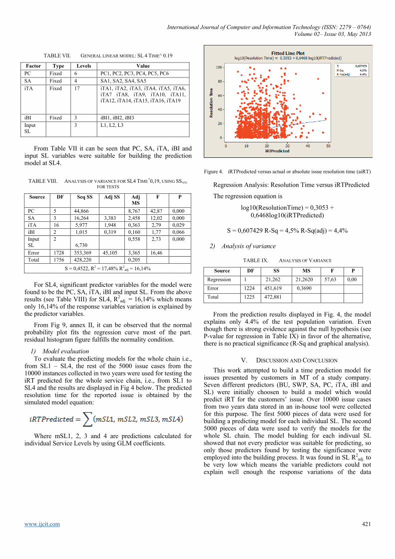
1) Model evaluation To evaluate the predicting models for the whole chain i.e.,

from SL1 – SL4, the rest of the 5000 issue cases from the 10000 instances collected in two years were used for testing the iRT predicted for the whole service chain, i.e., from SL1 to SL4 and the results are displayed in Fig 4 below. The predicted resolution time for the reported issue is obtained by the simulated model equation:

Where mSL1, 2, 3 and 4 are predictions calculated for individual Service Levels by using GLM coefficients.

Figure 4. iRTPredicted versus actual or absolute issue resolution time (aiRT)

Regression Analysis: Resolution Time versus iRTPredicted

The regression equation is

log10(ResolutionTime) = 0,3053 + 0,6468log10(iRTPredicted)

S = 0,607429 R-Sq = 4,5% R-Sq(adj) = 4,4%

2) Analysis of variance

TABLE IX. ANALYSIS OF VARIANCE

Source DF SS MS F P

Regression 1 21,262 21,2620 57,63 0,00

Error 1224 451,619 0,3690

Total 1225 472,881

From the prediction results displayed in Fig. 4, the model explains only 4.4% of the test population variation. Even though there is strong evidence against the null hypothesis (see P-value for regression in Table IX) in favor of the alternative, there is no practical significance (R-Sq and graphical analysis).

V. DISCUSSION AND CONCLUSION

This work attempted to build a time prediction model for issues presented by customers in MT of a study company. Seven different predictors (BU, SWP, SA, PC, iTA, iBI and SL) were initially choosen to build a model which would predict iRT for the customers’ issue. Over 10000 issue cases from two years data stored in an in-house tool were collected for this purpose. The first 5000 pieces of data were used for building a predicting model for each individual SL. The second 5000 pieces of data were used to verify the models for the whole SL chain. The model bulding for each indivual SL showed that not every predictor was suitable for predicting, so only those predictors found by testing the significance were employed into the building process. It was found in SL R2

adj. to be very low which means the variable predictors could not explain well enough the response variations of the data


www.ijcit.com

422

collected for building the models. SL2 had the highest R2adj =

17,13% and SL3 had the lowest R2adj = 5,78%. The whole SL

chain i.e from SL1-SL4 had even worse R2adj = 4.4%. So it can

be concluded that the variable predictors selected for building the iRT model explains only 4.4% of the response variations in the model. In practice this model cannot be used in the real world. However, the method and methodology applied to research the iRT variables can be used in future when more factors concerning the parameters explaining the variables are found. In order to improve the model predictive accuracy, further research will be done by investigating other factors and variables that will improve the prediction effectiveness. Among other things that are to be analyzed is the hardware (HW) of the products e.g. the printed wire board, as these might be of different versions at different stages of the life of the product. HW implies a circuit board where all components forming a product are surface mounted or soldered. The same goes for the software versions including the variant software which are specific for a specific customer. Another factor that might have an influence on iRT is the samples for verifying an issue. Time to receive samples for verifying an issue is not always predictable due to different custom regulations in different countries and for issue resolvers it takes a long time to receive the samples [22]. The iBI is subjective; it is likely to vary from person to person. Deeper subgrouping of the iTA would be worth investigating. Another issue that should be investigated is to find the way of working in each SL and note some practices or other work operating modes which differs from the assumed standard normal working routine.

REFERENCES [1] Lewis-Beck, M.S. Election Forecasting Principles and Practice. BJPIR:

Vol. 7 Issue 2, pg. 145-164, May 2005

[2] Mentzer, J., Cox J. (1984). “Familiarity, Application and Performance of Sales Forecasting Techniques.” Journal of Forecasting, Summer 1984, 27-36.

[3] Shahabuddin, S. “ Forecasting techniques for production schedule” Proceedings of the American Society of Business and Behavioral Sciences, Volume 7, Number 9 Las Vegas, 2000, 70-77

[4] Makridakis, Spyros. Winkler, R.L. “Average of Forecasts: Some Empirical Results” Management Science, September 1983, Vol. 29, No 9 p. 987

[5] Bates, J.M., Granger, C.W. J. “The combination of Forecasts” Operational Research Quaterly, 1969, Vol. 20 pg 451

[6] Armstrong, J.S. Combining Forecasts: The End of the Beginning or the Beginning of the End?* Published in International Journal of Forecasting (1989), 5, 585-588

[7] Mahmoud, E. “Accuracy in Forecasting: A Survey” Journal of Forecasting, April/June 1984, Vol. 3 p. 139

[8] Makridakis, S., & Hibon, M. (2000). The M3-Competition: results, conclusions and implications, International Journal of Forecasting, 16, p. 459

[9] Roos, I. “Switching Process in Customer Relationship” Journal of Service Research 1999 Vol. 15 pp 68-85

[10] Berry, L. L., Parasuraman, A., Zeithaml, V.A “Improving service quality in America: Lessons learned” Academy of Management Executive, 1994 Vol. 8 No. 2

[11] Kasper, H., Lemmikk, J., “After Sales Service quality: Views Between Industrical Customers and Service Managers” Industrial Marketing Management, 1989 Vol. 18 pp. 199-208

[12] McCollough, M.A., Berry, L.L., Yadav, M.S., “An Emperical Inestigation of a Customer Satisfaction after Service Failure and Recovery” Journal of service Research 2000 Vol. 3

[13] Singh, J., Wilkes, R.E., “When consumers complain: A path analysis of the key antecedents of consumer compliant response estimates”. Journal of the Academy of Marketing Science, 1996 Vol. 24 Issue No. 4 pp. 350-365

[14] Tax, S.S., Brown, S.W., “Recovering and Learning from Service Failure” Sloan Management Review, 1998 Vol. 3. Eason, B. Noble, and I. N. Sneddon, “On certain integrals of Lipschitz-Hankel type involving products of Bessel functions,” Phil. Trans. Roy. Soc. London, vol. A247, pp. 529–551, April 1955. (references)

[15] Fonell, C., Westbrook, R.A., “The vicious circle of consumer complaints.” Journal of Marketing, Vol. 48 Summer 1984 pp 68-78

[16] Resnick, A.J., Harmon, R.R., “Consumer complaints and managerial response: A holistic approach “ Journal of Marketing 1983, Vol. 4 pp 86-97

[17] Smith, A.K., Bolton, R.N., Wagner, J., “A model of customer satisfaction with service encounters involving failure and recovery.” Journal Marketing Reseach, Vol. xxxvi August 1999, pp 356-372

[18] Hansen, S.W., Swan, J.E., “Modeling industrial buyer complaints: Implications for satisfying and saving customers.” Journal of Marketing theory. 1997 Vol 5 Issue 4 , pp 12-21

[19] Mwegerano, A., Kytösaho, P., Tuominen, A., “Characterization of Resolution Cycle Times of Corrective Actions in Mobile Terminals”. Journal of Quality and Reliability Engineering International. 2008 Vol. 24 pp. 613-621

[20] Schbrowsky, J.A., Lapidus, R.S., “Gaining a competitive advantage by analyzing aggregate complaints.” Journal of consumer marketing. Vol 11 Issue 1 1994, pp 15-26

[21] Mwegerano, A., Kankaaranta, J., Hämeenoja, O., Suominen, A., ”Perceived after Sales Service: Communication within the Service Chain” . Quality Technology & Quantitative 2012. Vol. 9 Issue No. 4 pp. 407-419

[22] Mwegerano, A., Kytösaho, P., Tuominen, A., ”Applying sel-organizing maps method to analyze the corrective action’s quality provided to customers with mobile terminals” iBusiness journal, 2012, Vol 4 pp 108-120


www.ijcit.com

423

ANNEX I. DESCRIPTIVE STATISTICS OF THE VARIABLES GATHERED

Figure 5. Pareto chart of the explanatory variables gathered for building the

iRT predicting model

ANNEX II. MODEL RESIDUAL FOR DIFFERENT SERVICE

LEVELS (SL)

0,80,40,0-0,4-0,8

99,99

99

90

50

10

1

0,01

Residual

Per

cent

1,11,00,90,80,7

0,50

0,25

0,00

-0,25

-0,50

Fitted Value

Res

idua

l

0,450,300,150,00-0,15-0,30-0,45-0,60

80

60

40

20

0

Residual

Freq

uenc

y

2000

1800

1600

1400

1200

100080

060

040

020

01

0,50

0,25

0,00

-0,25

-0,50

Observation Order

Res

idua

l

Normal Probability Plot Versus Fits

Histogram Versus Order

Residual Plots for L1Time^0.09

Figure 6. Model Residual for SL1

1,00,50,0-0,5-1,0

99,99

99

90

50

10

1

0,01

Residual

Per

cent

1,201,050,900,750,60

1,0

0,5

0,0

-0,5

Fitted Value

Res

idua

l

0,80,60,40,20,0-0,2-0,4-0,6

160

120

80

40

0

Residual

Freq

uenc

y

2000

1800

1600

1400

1200

100080

060

040

020

01

1,0

0,5

0,0

-0,5

Observation Order

Res

idua

l




Figure 7. Model residual for SL2

1,00,50,0-0,5-1,0

99,99

99

90

50

10

1

0,01

Residual

Per

cent

1,201,151,101,051,00

0,5

0,0

-0,5

-1,0

Fitted Value

Res

idua

l

0,60,40,20,0-0,2-0,4-0,6-0,8

80

60

40

20

0

Residual

Freq

uenc

y

2000

1800

1600

1400

1200

100080

060

040

020

01

0,5

0,0

-0,5

-1,0

Observation Order

Res

idua

l




Figure 8. Model residual for SL 3

210-1-2

99,99

99

90

50

10

1

0,01

Residual

Per

cent

2,01,51,0

1

0

-1

-2

Fitted Value

Res

idua

l

1,20,80,40,0-0,4-0,8-1,2-1,6

200

150

100

50

0

Residual

Freq

uenc

y

2000180016001400120010008006004002001

1

0

-1

-2

Observation Order

Res

idua

l




Figure 9. Model residual for SL4

Predicting Customers Issues Resolution Times in Mobile ... · PDF filePredicting Customers...

Documents

Transcript of Predicting Customers Issues Resolution Times in Mobile ... · PDF filePredicting Customers...