PRECISION ENGINEERING

CENTER

2004 ANNUAL REPORT VOLUME XXII

March 2005

Sponsors: 3M Corporation Los Alamos National Laboratory Missile Defense Agency National Science Foundation Optical Research Associates Precitech Precision, Inc. Sandia National Laboratory Vistakon, Johnson & Johnson Vision Care Inc.

Faculty: Thomas Dow, Editor Phillip Russell Greg Buckner Ronald Scattergood Jeffrey Eischen David Youden Paul Ro

Graduate Students: David Brehl Lucas Lamonds Brett Brocato Witoon Panusittikorn Nathan Buescher Travis Randall Karalyn Folkert Nadim Wanna Karl Freitag Robert Woodside Simon Halbur Yanbo Yin Tim Kennedy

Undergraduate Students: Anthony Wong

Staff: Kenneth Garrard Alexander Sohn Lara Masters

TABLE OF CONTENTS

SUMMARY i

DESIGN 1. Design Tools for Freeform Optics 1 by K.P. Garrard and T.A. Dow 2. Surface Deconvolution for Diamond Turning 24 by W. Panusittikorn, K.P. Garrard, and T.A. Dow

FABRICATION 3. TEM and Raman Spectroscopic Analysis of High Pressure Phase 51 Transformations in Diamond Turned Single Crystal Silicon by T. Kennedy, T. Randall and R. Scattergood 4. Micromachining Using EVAM by B. Brocato, A. Sohn, and T.A. Dow 60 5. Live- Axis Turning by N. Buescher, A. Sohn, and T.A. Dow 90

METROLOGY 6. Metrology Artifact Design by K. Folkert and T.A. Dow 113 7. Fast Tool Servo Measurement by A. Wong and T.A. Dow 131

ACTUATION 8. Non-Contact Transportation Using Flexural Ultrasonic Wave by Y. Yin and P.I. Ro 141

CONTROL 9. Two-Axis Force-Feedback Deflection Compensation of Miniature Ball End Mills by K. Freitag, A. Sohn, G. Buckner, and T.A. Dow 158

PEC PHOTO 177 PERSONNEL 179 GRADUATES OF THE PRECISION ENGINEERING CENTER 191 ACADEMIC PROGRAM 197 PUBLICATIONS 204

i

SUMMARY The goals of the Precision Engineering Center are: 1) to improve the understanding and capability of precision metrology, actuation, manufacturing and assembly processes; and 2) to train a new generation of engineers and scientists with the background and experience to transfer this new knowledge to industry. Because the problems related to precision engineering originate from a variety of sources, significant progress can only be achieved by applying a multidisciplinary approach; one in which the faculty, students, staff and sponsors work together to identify important research issues and find the optimum solutions. Such an environment has been created and nurtured at the PEC for over 22 years; the new technology that has been developed and nearly 100 graduates attest to the quality of the results. The 2004 Annual Report summarizes the progress over the past year by the faculty, students and staff in the Precision Engineering Center. During the past year, this group included 7 faculty, 13 graduate students, 1 undergraduate student, 2 full-time technical staff members and 1 administrative staff member. Representing two different Departments from the College of Engineering, this diverse group of scientists and engineers provides a wealth of experience to address precision engineering problems. The format of this Annual Report separates the research effort into individual projects; however, this should not obscure the significant interaction that occurs among the faculty, staff and students. Weekly seminars by the students and faculty provide information exchange and feedback as well as practice in technical presentations. Teamwork and group interactions are a hallmark of research at the PEC and this contributes to both the quality of the research as well as the education of the graduates. The summaries of individual projects that follow are arranged in the same order as the body of the report, that is the five broad categories of 1) design, 2) fabrication, 3) metrology, 4) actuation and 5) control. 1) DESIGN The emphasis of the metrology projects has been to develop new techniques that can be used to predict surface shape as well as measure important parameters such as tool force. Design Tools For Freeform Optics Freeform optical surfaces can be used to control astigmatism at multiple locations in an image. As a result, a freeform surface may replace multiple spherical and aspheric reflective components in a complex optical system. Unfortunately, designers have been reluctant to use freeform or even aspheric surfaces, in most systems, because of the difficulty of obtaining optics that meet form and finish requirements at acceptable cost. A project is in progress with Optical Research Associates (ORA), the producers of CODE V, to remedy this obstacle by providing feedback to the designer on the manufacturability of an optical surface as part of the design

ii

process. Additional parameters such as surface sag, relative cost estimates and allowable form errors can now be included in the system optimization process. Surface Deconvolution for Diamond Turning Free-form optical systems can be fabricated using a Diamond Turning Machine (DTM) and a Fast Tool Servo (FTS). The DTM creates the rotationally symmetric component and the FTS simultaneously adds the Non-Rotationally Symmetric (NRS) component to create the desired surface shape. Synchronization between the DTM axes and the FTS is critical if the correct freeform shape is to be produced. The errors caused by the FTS dynamics can be corrected if they are known, repeatable and used to modify the input command to the actuator. The concept for determining the modified input command is known as deconvolution and is a standard element of digital signal processing. It is a form of feed-forward control, but the entire tool path is used to create the modified signal rather than the current value. As a result, the command is not related to the position feedback, so there is no delay in the response. Two demonstrations are presented, an off-center sphere and a cosine wave. For each shape, the surface produced was dramatically improved when compared with the uncompensated shape. 2) FABRICATION Fabrication of precision components is an emphasis area for the PEC. Current projects include machining of single crystal silicon, MEMS devices and freeform optics. Analysis Of High Pressure Phase Transformations in Single Crystal Silicon Diamond cubic silicon (Si-I) is a brittle material under standard temperature and pressure, but when exposed to a high pressure environment, the crystal structure transforms into a ductile ®-tin metallic phase (Si-II). Once the Si-II is unconstrained, it back-transforms into multiple forms of Si, mainly amorphous Si (a-Si) and Si-I. This transformation allows silicon to be machined without brittle fracture occurring, but the back transformation alters the surface (~500 nm in depth). ßIn situ analysis of this transformation during the manufacturing process is impractical. Using transmission electron microscopy (TEM), specifically cross sectional TEM (XTEM) and Raman spectroscopy, a portrait can be formed of how and why the transformations occur. Micromachining using EVAM The goal of this research is to demonstrate Elliptical Vibration Assisted Machining (EVAM) as a 3-D micro-structuring tool for MEMS applications. While many MEMS (MicroElectroMechanicalSystems) devices are fabricated using silicon etching techniques developed for the microelectronics industry, micro-machining is an attractive alternative because of its low start-up cost relative to other capital-intensive MEMS technologies, applicability to a wide range of materials, high flexibility of feature geometry and low cost for prototype manufacturing. The Ultramill Elliptical Vibration Assisted Machining (EVAM) system has unique capabilities among micro-machining techniques. Its features include zero runout and a

iii

tunable vibrating tool path. Three-dimensional structures with 15 µm plan-view features, 500 nm elevation features, and 20 nm RMS surface finish have been achieved on a 200 µm part scale. Live Axis Diamond Turning The term Live-Axis turning (LAT) has been coined to describe a lightweight, linear-motor driven, air bearing slide that can be used to fabricate non-rotationally symmetric optical components. The system described is the result of a joint effort by the PEC and Precitech to create a long-range fast tool servo to fabricate future NASA optics. The slide uses a triangular cross-section, lightweight (0.6 Kg) honeycomb aluminum piston driven by a linear motor (27 N maximum force) resulting in an acceleration capability of 45 g. The LAT axis has been mounted on a Nanoform 600 diamond turning machine and both flat surfaces and tilted flat surfaces have been machined. The flat surfaces had surface finishes of 75 nm rms and the tilted flat surfaces, using a maximum stroke of ±2 mm at 20 Hz, had a surface finish of 240 nm rms. Current efforts are centered on the control system to improve the surface finish and figure error. 3) METROLOGY Metrology is at the heart of precision engineering – from measuring fabricated parts to calibration artifacts to dynamic system characterization. Several of these areas have been addressed in research programs. Metrology Artifact Design After a part has been manufactured, the part is measured to determine whether it is within its tolerance region. These measurements are often taken on Coordinate Measuring Machines (CMMs). Traditionally, a calibration artifact determines the static influences of the machine such as machine geometry. The goal of this project is to design and fabricate a calibration artifact that will test the CMM dynamically and determine the effects of those influences. The artifact developed is a ring gauge to represent the typical size of parts manufactured by the Y-12 National Security Complex (Y-12). On the ring gauge, small swept sine wave features are placed on the inside and outside diameter. A swept sine wave is a sine wave that continuously varies its frequency. The range of frequencies creates a window for evaluation of the machine capabilities. By knowing the magnitude and phase characteristics of the dynamic system, the operator can make decisions referring to the machine’s capabilities based on the measurement speed. Fast Tool Servo Dynamic Performance Measurement Getting the most from an actuator is the goal of most servo designs. However as the operating frequency increases, gain and phase issues change the actual motion of the actuator from the desired path. Deconvolution techniques seek to identify the dynamics of the actuator and find a modified signal, that when sent through the actuator, will produce the desired path. The

iv

deconvolution algorithm requires accurate knowledge of the system dynamics; that is, the gain and phase of the outlet motion compared to the inlet command for an open-loop or a closed loop system. This section describes a method developed to find the dynamics of a Variform fast tool servo (FTS). A LabView program was developed to generate the appropriate range of input frequencies and amplitudes, send commands to the Variform, collect the resulting motion data and generate the system dynamics. 4) ACTUATION Implementation of techniques to move or control the position of an object requires a well-characterized actuator that fits the range and resolution of the application. In the past, emphasis has been placed on actuators for real-time control, but other applications such as transporting components for assembly are equally important. Non-Contact Transportation using Flexural Ultrasonic Wave A new non-contact transportation system is being designed at the Precision Engineering Center. The system is based on NFAL (Near-Field Acoustic Levitation) and near boundary streaming. In this report, background knowledge is introduced about applications of NFAL and near boundary streaming. Two experiments have been set up at the PEC, one is to check the validity of NFA, and the other is to design a non-contact transportation system. Theoretical approaches are then introduced and finite element analysis is used to conduct modal and transient analysis. 5) CONTROL Control of a precision fabrication processes involves both the characterization of the electromechanical system and the selection of hardware and software to implement the control algorithm. Two-Axis Force-Feedback Deflection Compensation Of Miniature Ball End Mills Correction for bending deflection of small (sub-millimeter diameter) milling tools was the focus of this project. This scheme was implemented on a high-speed, air-bearing spindle capable of speeds up to 60,000 rpm. This spindle was suspended on a pair of load cells and the real-time cutting force in two dimensions was determined based on the readings of each load cell and knowledge of the dynamic response of the spindle. Measurements from the two load cells can be combined to produce accurate (+/- 0.2 N) cutting force estimates. The load cell supported spindle was mounted on flexure guided piezoelectric actuators that incorporated closed loop capacitance gage feedback for position commands. This system can respond to the real-time cutting forces on the tool and produce the appropriate motion to compensate for tool deflection errors in two orthogonal directions. Through the use of this self-contained spindle actuator and force measurement system, form errors were reduced from 10-15 µm for a fixed spindle to 2-3µm using closed loop force feedback. An overall reduction of 75% in form error was achieved thru the implementation of force feedback machining.

1

1 DESIGN TOOLS FOR FREEFORM OPTICS

Kenneth P. Garrard Alexander Sohn

Precision Engineering Center Staff Thomas A. Dow

Professor Department of Mechanical and Aerospace Engineering

Freeform optical surfaces can be used to control astigmatism at multiple locations in an image. As a result, a freeform surface may replace multiple spherical and aspheric reflective components in a complex optical system. Unfortunately, designers have been reluctant to use freeform or even aspheric surfaces in most systems because of the difficulty of obtaining optics that meet form and finish requirements at acceptable cost. A project is under way with Optical Research Associates (ORA), the producers of CODE V, to remedy this obstacle by providing feedback to the designer on the manufacturability of an optical surface as part of the design process. Additional parameters such as surface sag, relative cost estimates and allowable form errors can now be included in the system optimization process.

2

1.1 INTRODUCTION Advanced optical systems play a pivotal role in military applications, including advanced optical telescopes and imaging LADARs (LAser Detection And Ranging). Optics provide the eyes for imaging, surveillance, detection, tracking and discrimination. Therefore, improvements in optical design and fabrication are important targets for research and development efforts. One such improvement is the inclusion of freeform elements in optical designs. A recent NASA imaging spectrometer (IRMOS) utilized freeform surfaces to help reduce the size of the system by an order of magnitude [1]. Significant reductions in size can dramatically reduce the use of exotic materials such as beryllium. The ensuing mass reductions provide enhanced performance for space systems and interceptors that require high accelerations in order to reach their targets at the correct point in trajectory. Freeform surfaces can also be used to control astigmatism at multiple locations in the field of view and thus reduce wavefront aberration. To make these advanced optical systems available for commercial and defense applications, an enhanced design environment is needed; one that gives the designer feedback on the manufacturability of the design as well as the optical performance. This environment needs a fundamentally new figure of merit to simultaneously predict optical performance and fabrication complexity. The core of this design environment is the subject of a Phase I STTR that has recently been funded by the Missile Defense Agency (MDA). The goal for this project is the creation of optical design software that, for the first time, optimizes both traditional optical performance measures and new manufacturing specific process metrics to leverage recent advances in design and fabrication capabilities for freeform optical components. Coupled with existing commercially available optical design capabilities, this new software will enable optical system designers to deploy cost effective freeform surface shapes (through minimization of optical design effort, manufacturing setup and machining time) for use in advanced multi-band (IR and visible) imagery systems. Designers will be able to create advanced optical systems to meet the evolving requirements of MDA while ensuring that they are producible. This project will combine the capabilities of the foremost optical design house, Optical Research Associates (ORA), with the unique freeform design, fabrication and metrology experience of the Precision Engineering Center (PEC). 1.2 OPTICAL DESIGN FOR MANUFACTURING This project involves the transfer of technology from the PEC to ORA with the goal of providing the optical designer with timely feedback on the manufacturing feasibility and cost of design options. By incorporating knowledge of the capabilities and limitations of fabrication technologies into the design optimization software, the class of available surfaces can be

3

extended to include freeform geometries. Initially, the scope of this work is limited to diamond machining with a fast tool servo and off-axis conic surfaces. 1.2.1 OPTICAL DESIGN The selection of elements and element locations for a new optical design is driven by optical performance and packaging requirements. The designer can employ reflective, refractive or diffractive elements whose shapes can be planar, spherical, aspheric or freeform. However, once an acceptable design is conceived, manufacturing and assembly issues determine its viability. The cost to change the design is lowest in the early stages and is increasingly expensive as the effort proceeds from concept to product. If the designer has feedback on the manufacturability of the elements early in the design process, the quality of the final design can be improved. For a design that consists of a series of spherical elements, a large body of information is available regarding manufacturability – material compatibility, geometry limitations, delivery and cost. Aspheric designs are less common, but fabrication capabilities to generate such surfaces are available. However, freeform surface fabrication capabilities are very limited. While some of the available optical software can deal with such shapes, no feedback is available to the designer on either the feasibility or the cost to create such a surface. Hence, most designers tend to avoid freeform shapes, even if they would simplify the design, reduce the number of components, improve the imaging performance, shorten the assembly time, and decrease the cost. 1.2.2 FABRICATION Freeform optical surfaces have no axis of symmetry and, as a result, this surface shape is a function of both radius (r) and angular position (θ). To produce such a surface, an additional degree of freedom is needed. This has been done by driving the machine tool axis as a function of r and θ (typically a big, heavy axis and thus the spindle speed must be low and production times tend to be long) or adding an auxiliary axis (Fast Tool Servo - FTS) to move the tool. Auxiliary axes can be obtained with strokes from 5 µm to several mm and operating frequencies from 1 KHz to 2 Hz respectively. A fast tool servo on a Diamond Turning Machine (DTM) is the most efficient way to produce freeform shapes in diamond turnable materials. The FTS can be programmed to create surfaces that are a function of DTM axes positions as well as the spindle angular position as illustrated in Figure 1. The shape of the freeform part can be divided into rotationally symmetric (RS) and non-rotationally symmetric (NRS) components as illustrated in Figure 2 and the decomposition can have a major impact on the fabrication process. The creation of these two components (not

4

necessarily unique) is a technical challenge that has been addressed at the Precision Engineering Center (PEC) at NC State University and will be incorporated in this project [2].

Figure 1. Coordinate system for machining an off-axis freeform surface with a fast tool servo.

(a) (b) (c) Figure 2. Off-axis conic segment (a), and its decomposition into symmetric (b) and non-symmetric (c) components for machining on-center. Note the 100x increase in amplitude scale for the non-symmetric component. The main axes of the DTM (X and Z) create the symmetric component (function of radius, r) while the FTS adds the non-symmetric component (function of angular location, θ, as well as radius, r). As the tool feeds from the outside of the part to the center, the linear axes of the lathe move the tool along the correct asphere (Figure 2b) and the fast tool servo simultaneously moves the tool in the W direction to add the (r, θ) component (Figure 2c) that will create the desired optical shape (Figure 2a). The range and bandwidth of the FTS will dictate the feed rate and maximum spindle speed, which will have a direct bearing on the time and cost to fabricate the surface.

5

1.2.3 ASTIGMATISM FROM OBLIQUE RAYS An optical wavefront acquires aberration, especially astigmatism, when it reflects obliquely off a curved mirror that is locally rotationally symmetric. This means that the surface is rotationally symmetric about the normal vector at a point intersected by the central ray in the beam. Because of the obliquity, the mirror appears to have more power in the direction of the field angle. A fan of rays in the plane of the field angle will focus closer to the mirror than a fan of rays in the orthogonal direction. The axial separation of the best focus for horizontal and vertical ray fans is a measure of astigmatism. For a locally rotationally symmetric mirror, a field angle whose chief ray is coaxial with the mirror axis (normal incidence) is the only field angle where there is no astigmatism. Otherwise, astigmatism increases as the square of the field angle. Controlling astigmatism in systems with off-axis fields can be accomplished by including one or more non-rotationally symmetric elements in the design. This usually results in a more compact optical layout as well.

tmc_aas.len Scale: 0.45 ORA 09-Jan-04

55.56 MM tmc_asp.len

ORA 09-Jan-04

FRINGE ZERNIKE PAIR Z5 AND Z6vs

FIELD ANGLE IN OBJECT SPACE

0.5waves

-2 -1 0 1 2

X Field Angle in Object Space - degrees

-2

-1

0

1

2

Y Field Angle in Object Space - degrees

tmc_aas.len

ORA 09-Jan-04

FRINGE ZERNIKE PAIR Z5 AND Z6vs

FIELD ANGLE IN OBJECT SPACE

0.5waves

-2 -1 0 1 2

X Field Angle in Object Space - degrees

-2

-1

0

1

2

Y Field Angle in Object Space - degrees

Figure 3. Optimized image quality for a 3-mirror anastigmat imager (left) has more than twice as much astigmatism across the full-field using symmetric surfaces (center) as can be achieved with freeform surfaces (right). 1.2.4 BENEFITS OF FREEFORM SURFACES To avoid astigmatism at a single off-axis field angle, what is needed is a locally anamorphic surface (i.e., not rotationally symmetric about the local surface normal), with a longer radius in the field angle direction than in the orthogonal direction. With an off-axis field, replacing a rotationally symmetric surface with a freeform surface allows the vertical and horizontal fans of rays to focus at the same point. Figure 3 shows a representative unobscured mirror system with associated astigmatism maps across the extended field of view for both the locally rotationally symmetric and freeform versions of the system. The length of the lines in the figure indicates the magnitude of the astigmatism. Note there are two nodes (points where the aberration is zero) in the field. In this illustration, one can zero out the astigmatism for two off axis field angles

6

(mirror images of each other), but for a range of field angles one cannot exactly zero the astigmatism. Distortion and coma also have this nodal behavior. Thus a key benefit of using freeform surfaces is that they offer the designer the ability to control both the number and position of aberration nodes within the field of view. This level of control allows us to reduce the worst-case wavefront aberration. 1.2.5 MODELING FREEFORM SURFACES There are at least two ways to model locally anamorphic power. One is to take an axially symmetric surface and add tilt, decenter, and asphericity. In that cas,e the vertex of the surface may be far off of the working aperture and the tilt angle may be large. However, it is simpler and more efficient to model the surface without such an extreme tilt and decenter. This can be accomplished by modeling the surface directly as an anamorphic function such as an aspheric toroid. This method of modeling can also help the fabrication process. The freeform surface can be thought of as decomposition into an axially symmetric surface plus NRS deformations. If the axis of symmetry, if the rotationally symmetric portion is in or near the working aperture, then fabrication is easier using a spindle-based method in which the part rotates about an included axis. 1.2.6 OPTIMIZATION MERIT FUNCTIONS When a freeform surface is to be utilized, the designer needs tools to evaluate the feasibility and cost of manufacture. The designer also requires techniques for quantifying these criteria, so they can be incorporated into an optimization strategy that permits simultaneous control of manufacturing issues and overall optical quality. The mathematical foundation for evaluating manufacturing cost has been developed at the PEC for off-axis conic surfaces to be machined on-center [3]. This algorithm decomposes the surface into a best-fit aspheric shape and a nonrotationally symmetric component that together create the required surface. The algorithm attempts to minimize the sag of the non-rotationally symmetric component to limit the dynamic range of the fast tool servo and maximize machining speed. In its current form, this software can be used to analyze an existing design, but it cannot be included in the optimization process to facilitate the generation of improved optical designs. The project objective is to create new software algorithms that tie together the mathematical surface decompositions for machining off-axis conic sections, that are machined on-center using a FTS, with the optical design environment using automated optimization techniques. To accomplish this, fundamental relationships must be discovered that will allow the creation of merit functions to be used within the optimization environment to produce the best (in terms of

7

manufacturability and cost) decomposition of the symmetric and asymmetric components of the desired surface shape. This research will quantify the freeform optical manufacturing processes and create a new capability in optical computer aided design (OCAD) software tools to support manufacturing. The software developed will be the foundation for a future effort to prototype a working optical system that includes freeform elements. The algorithms and design environments to be explored during this effort will assist an optical designer in the development of freeform optical components by providing timely feedback on the feasibility of fabrication. The class of optics to be addressed is freeform optics that can be machined using a fast tool servo. The software will:

• Provide feedback on the FTS range of motion required to machine the optical surface, • Compare the range to available diamond turning machine systems, • Estimate the fabrication time, • Incorporate manufacturing parameters into the optical optimization process, • Produce output files that decompose the surface into best-fit asphere and NRS parameters

suitable for downloading to a manufacturing process, and • Estimate machining errors associated with the chosen process for fabrication.

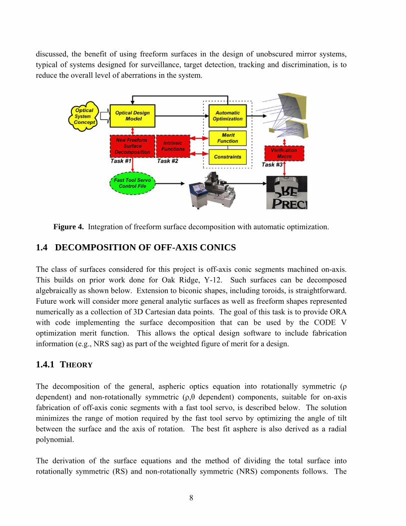
1.3 PLAN OF WORK The project will develop an integrated design and optimization environment that brings together, for the first time, the existing optical performance predictions with automated feedback of manufacturing costs of FTS machined freeform surfaces. Schematically, the project will create the environment shown in Figure 4. The proposed work plan is intended to prove the feasibility of practical and cost effective use of freeform surfaces for off-axis systems, where such surfaces would produce substantially less spherical aberration, astigmatism, distortion, coma and higher order aberrations such as trefoil and oblique spherical aberration. These surfaces would also enable the design of systems with lower overall wavefront error. To accomplish this goal, algorithms to enable process-aware optimization of optical performance will be created by first decomposing freeform surfaces into axially symmetric and anamorphically deformed component shapes and then controlling those shapes using manufacturing metrics though a set of intrinsic functions. Once this task is completed, novel verification and visualization methods must be created that will quantify the quality of the resulting surface manufacture. Each of these accomplishments will require innovation. The technical risks of creating a viable design and manufacturing process that will provide the imaging benefits of freeform surfaces are substantial, due primarily to the challenge of developing metrics that quantify the manufacturing impacts in ways that allow the metrics to be used effectively with existing, highly quantitative metrics such as image quality. As

8

discussed, the benefit of using freeform surfaces in the design of unobscured mirror systems, typical of systems designed for surveillance, target detection, tracking and discrimination, is to reduce the overall level of aberrations in the system.

Figure 4. Integration of freeform surface decomposition with automatic optimization. 1.4 DECOMPOSITION OF OFF-AXIS CONICS The class of surfaces considered for this project is off-axis conic segments machined on-axis. This builds on prior work done for Oak Ridge, Y-12. Such surfaces can be decomposed algebraically as shown below. Extension to biconic shapes, including toroids, is straightforward. Future work will consider more general analytic surfaces as well as freeform shapes represented numerically as a collection of 3D Cartesian data points. The goal of this task is to provide ORA with code implementing the surface decomposition that can be used by the CODE V optimization merit function. This allows the optical design software to include fabrication information (e.g., NRS sag) as part of the weighted figure of merit for a design. 1.4.1 THEORY The decomposition of the general, aspheric optics equation into rotationally symmetric (ρ dependent) and non-rotationally symmetric (ρ,θ dependent) components, suitable for on-axis fabrication of off-axis conic segments with a fast tool servo, is described below. The solution minimizes the range of motion required by the fast tool servo by optimizing the angle of tilt between the surface and the axis of rotation. The best fit asphere is also derived as a radial polynomial. The derivation of the surface equations and the method of dividing the total surface into rotationally symmetric (RS) and non-rotationally symmetric (NRS) components follows. The

9

general equation of an optical surface of revolution about the z axis can be written in Cartesian coordinates as,

( )( ) L+ρa+ρa+ρa+ρc+k+

cρ=z 83

62

4122

2

111 − (1)

where 222 y+x=ρ and c is the curvature of the conic at its vertex. The ai's are coefficients of an aspheric deformation polynomial. The constant, k, is related to the eccentricity of the conic and defines its shape as shown in Table 1.

Table 1. The Conic Constant

Surface k

Hyperboloid k < -1

Paraboloid k = -1

Ellipse (prolate, rotated about the major axis) -1 < k < 0

Sphere k = 0

Ellipse (oblate, rotated about the minor axis) k > 0

The geometry of the off-axis segment and its orientation in the parent coordinate system are shown in Figure 1(a). Fabrication of a segment of this surface by on-axis turning requires three coordinate transformations: translation so that the center of the surface is on-axis (i.e., coincident with the rotational axis), a cylindrical coordinate transformation that rewrites Equation (1) in terms of ρ and θ instead of x and y, and a tilt in the xz plane that minimizes the NRS sag after subtraction of the best-fit asphere. Only the first term in Equation (1) needs to be considered by the decomposition process as the aspheric deformation in terms of even radial powers can be added to the best-fit asphere. These transformations describe the surface in cylindrical coordinates as show in Equation (2).

( ) ( ) ( )θd+ρd+θρd+dθρd+d=z 2

62

54321 coscoscos − (2)

Equation (2) gives the value of z as a function of the radius from the spindle axis (ρ) and the rotational angle (θ) of the spindle. It consists of a rotationally symmetric component and a non-

10

rotationally symmetric component. The di's in Equation (2) are constants, which are defined by Equations (3-8) and depend upon the conic constant, k, the off-axis translation parameters, (x0, z0) and the tilt angle of the surface. The initial selection of the tilt angle is the tangent of the parent conic at the center of the segment. A simple iterative process generates an optimal angle with respect to the sag of the NRS surface.

( ) ( ) ( ) ( ) ( )( )α2

001 cos1

cos1cos/1sink+

αz+kαc+αx=d − (3)

( ) ( )( )α22 cos1

sincosk+

ααk=d − (4)

213 d=d (5)

( ) ( ) ( ) ( ) ( )[ ]( )α2

00214 cos1

sin1sin/1cos22k+

αz+k+αcαxdd=d −− (6)

( )α25 cos11

k+=d − (7)

( )( )α2

2226 cos1

sink+

αkd=d − (8)

Once an acceptable value for α is determined, the two components of the surface shape can be written as variations of Equation (2). The RS part will be the value of z at θ = π/2 and the NRS part will be the difference between the value of z from Equation (2) and the RS part. The evaluation of Equation (2) is problematic due to the subtraction of two very large but nearly equal quantities. A further simplification is possible that solves this loss of precision problem. It also reduces the evaluation time of the function by approximating the square root operation with a polynomial expansion. Substituting Equation (5) into Equation (2), the value of z can be rewritten as,

( ) ( ) ( )θρρθρθ 22

3

62

3

5

3

4121 coscos1cos

dd

dd

dddddz +++−+= (9)

The terms under the radical can be approximated using a binomial expansion with p = 1/2.

( ) ( ) ( )( )L+

−−+

−++=+ 32

!321

!2111 xpppxpppxx p (10)

The final simplified form of Equation (2) is now,

( ) ⎥⎦⎤

⎢⎣⎡ +−+−−≅ 5432

12 2567

1285

161

81

21cos EEEEEddz θρ (11)

11

where E is given by,

( ) ( )θρρθρ 22

3

62

3

5

3

4 coscosdd

dd

ddE ++= (12)

Equations (11) and (12) can be used to calculate surface heights over any (ρ,θ) grid needed by the optical design and optimization software. Numeric problems are avoided by calculating the truncated series in Equation (11) using Horner’s rule. More terms of the power series can be used to increase the accuracy of the calculation to any desired precision. This implementation can also be used to generate the reference data needed to fabricate the optic; either as a lookup table or in a real-time as a trajectory generator in the machine tool controller. 1.4.2 IMPLEMENTATION To transfer the decomposition procedure to ORA for incorporation into CODE V, a C program was written that implements the decomposition process and generates a vector of data points on either the conic surface, the RS component or the NRS component. Inputs are the number of radial and angular increments, the aperture (i.e., circular diameter), conic constant, radius of curvature at the center of the aperture and the radial distance from the center of the aperture to the origin. The output vector can be in Cartesian or cylindrical coordinates. In addition the NRS sag, best-fit asphere sag, an asphere error estimate and the asphere coefficients are produced. The asphere error estimate is the maximum sag between the true aspheric curve and the line segment approximation obtained by joining the radial output points. The program code listed in the appendix has been included in a beta version of CODE V as an external DLL. This facilitates future expansion to other surface types and decomposition algorithms. 1.5 VERIFICATION AND SIMULATION OF SURFACE FABRICATION One of the tasks of this project is to evaluate different machining processes for optical surfaces during the design phase to provide the designer with some feedback on manufacturability for the optical system. In its simplest form, this comes down to a cost/performance tradeoff. 1.5.1 COST The intention is not to provide a specific price quote and wholesale simulation of all the errors in a surface. Rather, the approach is more general in that a relative cost scale determined by setup time, consumables cost and machine time. In the initial cost estimate, items such as alignment, fixturing and programming are considered as factors.

12

1.5.2 PROCESSES Several fabrication processes will be considered for each part. Table 1 shows an assessment of performance and cost for each of the considered processes. Bandwidth is a measure of the maximum frequency at which NRS features can be generated. NRS Range gives the maximum excursion of the device at low frequency. Most of these systems cannot reach the maximum excursion at the bandwidth limit. The cost/time is a relative measure of how much it costs to operate the machine. This quantity includes initial purchase and setup costs, operator, maintenance, and cost of the accommodations/support equipment. The cost/area quantity is based on the amount of time necessary to set up and machine a part on the equipment.

Table 2. Cost/Performance assessment of various machining systems.

1.5.3 ASSESSMENT OF TYPICAL FABRICATION ERRORS One of the goals of this project is to provide feedback to the designer on what errors a particular fabrication process will generate in the surface. These errors are separated into two distinct categories: roughness and figure errors. Roughness The roughness of a diamond turned surface is typically limited by two factors: material effects and machine vibration. This assumes that other factors that can cause excessive roughness such as tool condition and theoretical finish are properly addressed in the turning process. Material effects such as grain size, brittle fracture, and inclusions have been thoroughly documented for common materials such as Aluminum, Copper, Electroless Nickel, Brass, PMMA, and Germanium to name a few. These materials will be placed in a database as part of the manufacturability along with their maximum finish ranges and will be combined with the

Process Vendor Bandwidth NRS Range Cost/time Cost/area Diamond Turning Various 0 0 $ $ FTS (PEC) 1kHz 38 µm $$ $ FTS 35 (Precitech) 900 Hz 35 µm $$ $ FTS 70 (Precitech) 700 Hz 70 µm $$ $ FTS 400 (Precitech,

Sterling) 300 Hz 400 µm $$ $$

Slow slide Servo (Moore Nanotech) 1 Hz 25 mm $$ $$$ Slow tool Servo (Precitech) 1 Hz 25 mm $$ $$$ Raster Flycutting (Precitech, Moore

Nanotech) 0.04 Hz 150 mm $$$ $$$$

13

machine database to provide finish feedback to the designer. This feedback will initially be supplied simply as an r.m.s. number which the designer can then enter into a scattering simulation outside the CODE V environment. Figure Errors Figure errors will be simulated so that their optical effects can be simulated in CODE V. Simulation of these errors will require a thorough analysis of their origin on one hand and a carefully chosen set of assumptions on the other. Sources of figure error seen in diamond turning are: tool centering, tool waviness, radius compensation, axis straightness, axis squareness, axis roll, pitch and yaw, synchronous spindle error motion, scale errors, and servo errors. Tool centering, tool waviness and radius correction are all manifestations of an error in the intended position of a point on the tool in relation to the part. To simulate these errors, a machining geometry must be chosen. In turning operations, location of the part in relation to the spindle axis is necessary to perform the simulation. The designer must therefore choose this parameter with the help of the decomposition. Once the surface has been located in the machine space, each point on the surface in an up to 640X480 point grid can be related to a tool position. For each tool position, the surface normals to the part are calculated and used to find the intended point of contact on the tool. For each of these contact points, an error due to centering, tool

Figure 5. Tool errors are calculated relative to a grid of surface points, which rotate about a point Pc. If there is an error in the location of the tool a distance X from this center of rotation and there is an error in the tool radius r as a function of contact angle γ, the intended contact point on the surface Pn will be relocated to P’n.

X

14

waviness, and radius correction is calculated. Centering error is simply a translation of each contact point in the X- and Y-directions. The magnitude of these errors is dependent on the centering method: optical or mechanical set station - 5µm, interferometer measurement – 1µm, AFM measurement – 100 nm. Each of these methods also has an associated cost function, but is unnecessary in the most expensive of fabrication methods – raster flycutting. Tool waviness is determined on the basis of a simulated radius variation of the tool as a function of tool contact angle. A database of several typical tool waviness profiles, in several grades (each associated with a cost function), is then used to calculate the error in the location of the tool contact point. This requires the calculation of the contact angle from the surface normals. These surface normals are also used to determine the error in the surface if, either, radius compensation was not performed, or if there is uncertainty in the determination of the tool radius. Waviness and radius compensation errors are factors considered here, including raster flycutting. All of these tool errors are then combined to produce a new surface map of the flawed, simulated surface before the next error simulation is performed. Geometric errors in the machine are simulated next in the machining system. The main sources of these errors are axis straightness, squareness, roll, pitch, and yaw as well as scale errors. All but the latter can be considered as purely a function of axis position and can be simulated from machine specs and the geometry of the machine. Scale errors, on the other hand, can vary over time as well as axis position. In addition to fixed deviations, scale errors are influenced by thermal changes in the machine base and laboratory environment. However, since thermal errors tend to vary slowly over time, typically on the order of minutes to hours, they cannot be considered dynamic errors and therefore belong into a class by themselves. Due to the difficulty in calculating thermal errors, they are determined by using measured data. Geometric errors, on the other hand, can be determined in a relatively straightforward way. Each machine axis has an associated position error profile in X, Y, and Z according to its straightness, roll, pitch, and yaw. While machine specifications usually only give magnitudes for these quantities, they normally have a sinusoidal form somewhere between ¼ and 1 period of a sine wave. This shape is thus applied to each of the error quantities, in a somewhat varied form, according to measured data. When the designer then chooses a machine to fabricate a surface, the position errors of the axes are then applied to the surface point array. Servo axis errors are the final type of error applied to the simulated surface. These are the dynamic errors of the servo, which reveal themselves in the form of amplitude and phase errors. These errors are dependent on the measured dynamics of each servo axis. A more responsive axis (higher bandwidth) will exhibit lower dynamic errors, but typically has less range than a more sluggish axis. Dynamic errors will only be applied to the NRS portion of the surface determined using decomposition. Again, each surface point will be shifted in amplitude and phase and combined with the previously calculated errors to reveal a simulation of what the surface would look like when produced with the method chosen by the designer. This modified

15

surface can then be reinserted into Code V to determine the impact of the machining process on the optical design. 1.6 CONCLUSIONS Decomposition software for off-axis conics has been transferred to ORA and included in the CODE V optical design package. This allows the user to see the impacts on the manufacturability of his or her design decisions. The addition of a cost/benefit assessment will greatly enhance the designer’s confidence in the manufacturability of free-form designs. REFERENCES 1. Garrard, K., A. Sohn, R. G. Ohl, R. Mink, V. J. Chambers. “Off-Axis Biconic Mirror

Fabrication”, Proceedings from the EUSPEN 2002 Annual Meeting (2002). 2. United States patent 5,467,675. Apparatus and method for forming a workpiece surface into

a non-rotationally symmetric shape. Thomas A. Dow, Kenneth P. Garrard, George M. Moorefield, II and Lauren W. Taylor (1995).

3. Allen, W.D., R.J. Fornaro, K.P. Garrard and L.W. Taylor. “A high performance embedded

machine tool controller”, Microprocessors and Microprogramming, 40, 179-191, (1994).

16

1.7 APPENDIX OFF-AXIS CONIC SURFACE DECOMPOSITION //------------------------------------------------------------------------// // // // Off-axis Conic Surface Decomposition for On-Axis Fabrication // // // // Copyright (c) 2004 North Carolina State University, // // Precision Engineering Center. // // // // All Rights Reserved. // // // // Written by Ken Garrard // // // //------------------------------------------------------------------------// // // nrsgen.c 10-29-2004 // #include <stdio.h> #include <stdlib.h> #include <float.h> #include <math.h> #pragma warn –aus // Useful constants #define nano_epsilon 0.000000001 #define pi 3.14159265358979323846264338327950288419716939937511 #define pi_two 1.57079632679489661923132169163975144204858469968755 #define two_pi 6.28318530717958647692528676655900576839433879875022 // Error return codes #define error_tilt 1 // Invalid [tilt_angle, conic_K] combination #define error_trans 2 // Invalid off-axis translation #define error_parms 3 // Invalid parameters [eg X0>R and K=0] // Surface type #define m_asphere 0 // Best fit asphere #define m_conic 1 // Conic segment translated on-axis #define m_nrs 2 // Non-rotationally symmetric residual #define def_surf m_nrs // Coordinate system #define m_cartesian 0 // Cartesian [x,y,z] #define m_cylinder 1 // Cylindrical [theta,rho,z] #define def_coord m_cartesian // Output control #define m_noheader 0 // Header info and surface data #define m_header 1 // Surface data vectors only #define def_header m_header #define def_n_radial 42 // Default output grid size #define def_n_angle 42 // Default off-axis conic segment #define def_conic_K -1.0 // Parabola #define def_aperture 127.0 // Aperture #define def_conic_R 2159.0 // Radius of curvature at vertex #define def_x_offaxis 300.0 // Off-axis distance // Command line argument help string #define help_str \ "\n" \ "nrsgen [-sanpchw] N M Ap K Rad X0\n\n" \ " s surface conic surface\n" \ " a asphere best fit asphere\n" \ " n nrs motion nrs decomposition\n" \ " p cylindrical coordinates (theta, rho, z)\n" \

17

" c cartesian coordinates (x, y, z)\n" \ " h include header info\n" \ " w supress header output\n\n" \ " arguments:: (use * as place-holder for default value)\n" \ " N radial increments, default = %ld\n" \ " M angular increments, default = %ld\n" \ " Ap aperture, default = %6.2lf\n" \ " K conic constant, default = %9.6lf\n" \ " Rad radius of curvature at center of aperture, default = %7.2lf\n" \ " X0 distance from origin to center of aperture, default = %7.2lf\n" // Output file header #define comment_str "//" #define header_str \ comment_str " nrsgen --> off-axis conic reference signal generation\n" \ comment_str " conic parameters::\n" \ comment_str " r = %lf\n" \ comment_str " K = %lf\n" \ comment_str " x0, z0 = %lf, %lf\n" \ comment_str " tilt = %12.10lf [%d]\n" \ comment_str " surface parameters::\n" \ comment_str " aperture = %lf\n" \ comment_str " # radial steps = %ld\n" \ comment_str " # angular steps = %ld\n" \ comment_str " decomposition results::\n" \ comment_str " nrs range = %10.7lf [%9.7lf to %#-9.7lf]\n" \ comment_str " asphere sag = %10.7lf\n" \ comment_str " asphere error = %10.7lf\n" \ comment_str " best-fit asphere polynomial coefficients::\n" // Output file column label strings #define cartesian_label comment_str "\n" comment_str " x y " #define cylinder_label comment_str "\n" comment_str " theta rho " #define conic_label " z\n" #define nrs_label " z_nrs\n" #define asphere_label " z_asphere\n" // Point data structure typedef struct s_point { double x, z; } t_point; // Line data structure, [Ax + By + C = 0] typedef struct s_line { double A, B, C; } t_line; // Argument mode structure typedef struct s_modes { int surf, // Surface type: conic, asphere, nrs coord, // Coordinates: cartesian, cylinrical header; // Text header: yes, no } t_modes; // Output file label vectors (indexed by mode.output and mode.surf) static char *coord_labels [] = {cartesian_label, cylinder_label}; static char *surf_labels [] = {asphere_label, conic_label, nrs_label}; // Error messages static char *error_strs [] = {"", "invalid [tilt,conic] combination", "invalid off-axis translation", "invalid parameters, surface does not exist"}; // Transformation results #define nterms 6 // Terms in approximation polynomials #define nsegs 100 // Intermediate segments in asphere fit static double conic_coeff [4]; // Conic transformation coefficients static double sqrt_coeff [nterms]; // Sqrt approximation coefficients static double asphere_coeff [nterms]; // Asphere polynomial coefficients

18

// Function prototypes // Command line argument parsing int next_iarg (int argi, int argc, char *argv [], int *ival); // integer double next_farg (int argi, int argc, char *argv [], double *fval); // float // Line creator and point-line distance function prototypes t_line mk_line (t_point *a, t_point *b ); double point_line_distance (t_point *pt, t_line *ln); // Surface generator int gen_surface (t_modes mode, int n_radial, int n_angle, double Wr, double K, double R, double X0); // On-axis transformation int init_gen (double R, double K, double X0, double Z0, double alpha); // On-axis tilt optimization int tilt_optmz (double R, double K, double X0, double Wr, double *Z0, double *alpha, int *ntilt); // NRS sag determination double nrs_range (double Wr, int n_radial, int n_angle, double *min_zp, double *max_zp); // Aspheric fit double asphere_fit (double Wr, int n_radial); // Point generation functions double gen_asphere (double rho, double theta); // Best fit asphere double gen_conic (double rho, double theta); // Conic segment double gen_nrs (double rho, double theta); // NRS component // Function pointer vector for variable surface generation (indexed by mode.surf) typedef double (*fp_surf) (double, double); fp_surf surf_fp[] = {gen_asphere, gen_conic, gen_nrs}; // Main // Parse input arguments, call gen_surface and print error message int main (int argc, char *argv []) { char *pch; // Character from argument string int argi = 1; // Argument vector index int rcode = 0; // Return code (0=no error) int n_radial = def_n_radial, // Number of radial steps n_angle = def_n_angle; // Number of angular steps double aperture = def_aperture, // Aperture conic_R = def_conic_R, // Conic radius conic_K = def_conic_K, // Conic constant (0=sphere,-1=parabola,...) x_offaxis = def_x_offaxis; // Distance from origin to center of aperture double Wr = def_aperture / 2.0; // Radius of circular aperture // Initialize mode vector with defaults t_modes mode = {def_surf, def_coord, def_header}; // Parse command line arguments if (argi < argc) if (*argv[argi] == '?') { // Respond to user request for help printf (help_str, n_radial, n_angle, aperture, conic_K, conic_R, x_offaxis); exit (0); } else if (*argv[argi] == '-') { // Process optional mode arguments for (pch = argv[argi++]+1; *pch != '\0'; pch++)

19

if (*pch == 's') mode.surf = m_conic; else if (*pch == 'a') mode.surf = m_asphere; else if (*pch == 'n') mode.surf = m_nrs; else if (*pch == 'p') mode.coord = m_cylinder; else if (*pch == 'c') mode.coord = m_cartesian; else if (*pch == 'h') mode.header = m_header; else if (*pch == 'w') mode.header = m_noheader; } // Parse and convert numeric arguments (if "*", keep default value) argi = next_iarg(argi, argc, argv, &n_radial ); argi = next_iarg(argi, argc, argv, &n_angle ); argi = next_farg(argi, argc, argv, &aperture ); argi = next_farg(argi, argc, argv, &conic_K ); argi = next_farg(argi, argc, argv, &conic_R ); argi = next_farg(argi, argc, argv, &x_offaxis); // Generate data on off-axis conic surface Wr = aperture / 2.0; rcode = gen_surface (mode, n_radial, n_angle, Wr, conic_K, conic_R, x_offaxis); // Output error message if (rcode > 0) printf("\nerror: %s\n", error_strs [rcode]); return (rcode); } // Convert next input command line argument to floating point double next_farg (int argi, int argc, char *argv[], double *fval) { if (argi < argc) { if (*argv[argi] != '*') *fval = atof(argv[argi]); ++argi; } return (argi); } // Convert next input command line argument to integer int next_iarg (int argi, int argc, char *argv[], int *ival) { if (argi < argc) { if (*argv[argi] != '*') *ival = atoi(argv[argi]); ++argi; } return (argi); } // Generate surface data for on-axis transformation of off-axis conic segment int gen_surface (t_modes mode, // Generator options int n_radial, // Number of radial increments int n_angle, // Number of angular increments double Wr, // Radius of off-axis segment double K, // Conic constant double R, // Radius of curvature double X0) // Distance to center of aperture { int ntilt; // Number of tilt optimizer iterations int rcode = 0; // Return code from function calls int j, k; // Loop indices double x, y, z; // Cartesian coordinates double theta, theta_incr; // Angular increment double rho, rho_incr; // Radial increment double Z0; // Z offset at center of aperture double alpha; // On-axis tilt angle double min_zp, max_zp; // Range of NRS motion double sag; // Asphere sag double max_error; // Maximum asphere curve error estimate // Find tilt angle that minimizes NRS motion if ((rcode = tilt_optmz(R, K, X0, Wr, &Z0, &alpha, &ntilt)) != 0) return (rcode); // Calculate NRS range of motion and asphere fit quality

20

sag = nrs_range (Wr, n_radial, n_angle, &min_zp, &max_zp); max_error = asphere_fit(Wr, n_radial); // Output header if (mode.header == m_header) { printf (header_str, R, K, X0, Z0, alpha, ntilt, (2.0 * Wr), n_radial, n_angle, fabs (max_zp - min_zp), min_zp, max_zp, sag, max_error); // Asphere coefficients for (k = 0; k < nterms; k++) printf ("%s A%02ld = %#-17.10lg\n", comment_str, (k + 1) * 2, asphere_coeff [k]); // Column labels printf ("%s%s", coord_labels [mode.coord], surf_labels [mode.surf]); } // Radial and angular increments rho_incr = Wr / n_radial; theta_incr = two_pi / n_angle; switch (mode.coord) { // Cylindrical coordinate output [theta, rho, z] case m_cylinder: for (j = 0, rho = Wr; j <= n_radial; j++, rho -= rho_incr) for (k = 0, theta = 0.0; k <= n_angle; k++, theta += theta_incr) { z = surf_fp [mode.surf] (rho, theta); printf (" %11.7lf %11.7lf %11.7lf\n", theta, rho, z); } break; // Cartesian coordinate output [x, y, z] case m_cartesian: for (j = 0, rho = Wr; j <= n_radial; j++, rho -= rho_incr) for (k = 0, theta = 0.0; k <= n_angle; k++, theta += theta_incr) { x = rho * cos(theta); y = rho * sin(theta); z = surf_fp [mode.surf] (rho, theta); printf (" %11.7lf %11.7lf %11.7lf\n", x, y, z); } break; } return (rcode); } // Make a line joining two points, find coefficients A,B,C of [Ax + By + C = 0] t_line mk_line (t_point *a, t_point *b) { t_line ln; if (a->x == b->x) {ln.A = 1.0; ln.B = 0.0; ln.C = -a->x;} // Vertical else if (a->z == b->z) {ln.A = 0.0; ln.B = 1.0; ln.C = -a->z;} // Horizontal else { ln.A = (b->z - a->z) / (b->x - a->x); // Slope = -A/B ln.B = -1.0; ln.C = a->z - ln.A * a->x; // Intercept = - C/B } return (ln); } // Calculate the distance between a point and a line double point_line_distance (t_point *pt, t_line *ln) { return (fabs(ln->A * pt->x + ln->B * pt->z + ln->C) / hypot(ln->A,ln->B)); } // Find coefficients to describe on-axis transformation of off-axis conic int init_gen (double R, double K, double X0, double Z0, double alpha)

21

{ int j; double d1, d2, d3, d4, d5, d6; double cos_a, sin_a, dd, dd1, d4t, rk, d51; cos_a = cos(alpha); sin_a = sin(alpha); dd = 1.0 + K * cos_a * cos_a; if (fabs (dd) < nano_epsilon) return (error_tilt); dd1 = 1.0 / dd; d1 = (X0 * sin_a + R * cos_a - (K + 1) * Z0 * cos_a) * dd1; if (fabs (d1) < nano_epsilon) return (error_trans); d2 = (-K * cos_a * sin_a) * dd1; d3 = d1 * d1; d4t = 2.0 * (X0 * cos_a - R * sin_a + (K + 1.0) * Z0 * sin_a); d4 = 2.0 * d1 * d2 - d4t * dd1; d5 = - 1.0 * dd1; d6 = d2 * d2 - (K * sin_a * sin_a) * dd1; conic_coeff [0] = d2; conic_coeff [1] = d4 / d3; conic_coeff [2] = d5 / d3; conic_coeff [3] = d6 / d3; d51 = d5 / (d1 * d1); sqrt_coeff [0] = - d1 * 0.5; asphere_coeff [0] = - (d5 / d1) * 0.5; for (j = 1; j < nterms; j++) { rk = (0.5 - j) / (j + 1); sqrt_coeff [j] = sqrt_coeff [j-1] * rk; asphere_coeff [j] = asphere_coeff [j-1] * d51 * rk; } return (0); } // Generate data point on conic surface double gen_conic (double rho, double theta) { int j; double tc, term, tz; tc = cos(theta); term = conic_coeff [1] * rho * tc + conic_coeff [2] * rho * rho + conic_coeff [3] * rho * rho * tc * tc; for (tz = 1.0, j = nterms - 1; j >= 0; j--) tz = term * (tz + sqrt_coeff [j]); tz += conic_coeff [0] * rho * tc; return (tz); } // Generate data point on best-fit asphere #pragma warn -par double gen_asphere (double rho, double theta) { int j; double tz, rr; rr = rho * rho; for (tz = 0.0, j = nterms - 1; j >= 0; j--) tz = rr * (tz + asphere_coeff [j]); return (tz); }

22

#pragma warn +par // Generate data point on residual NRS surface double gen_nrs (double rho, double theta) { return (gen_conic(rho, theta) - gen_asphere(rho, theta)); } // Find tilt angle that minimizes NRS range int tilt_optmz (double R, double K, double X0, double Wr, double *Z0, double *alpha, int *ntilt) { int rcode = 0; double dz0, sag, aperture; if ((dz0 = 1.0 - ((K + 1.0) * (X0 * X0) / (R * R))) < 0.0) return (error_parms); *Z0 = (X0 * X0) / (R * (1 + sqrt(dz0))); *ntilt = 0; aperture = 2.0 * Wr; *alpha = atan2 (*Z0, X0); do { ++(*ntilt); if ((rcode = init_gen (R, K, X0, *Z0, *alpha)) != 0) break; sag = gen_conic(Wr, 0.0) - gen_conic(Wr, pi); *alpha += atan2(sag, aperture); } while (fabs (sag) >= nano_epsilon); return (rcode); } // Find NRS range and asphere sag double nrs_range (double Wr, int n_radial, int n_angle, double *min_zp, double *max_zp) { int j, k; double z_asphere, z, rho, rho_incr, theta, theta_incr; *min_zp = DBL_MAX; *max_zp = DBL_MIN; rho_incr = Wr / n_radial; theta_incr = two_pi / n_angle; for (j = 0, rho = Wr; j <= n_radial; j++, rho -= rho_incr) { z_asphere = gen_asphere(rho,0.0); for (k = 0, theta = 0.0; k <= n_angle; k++, theta += theta_incr) { z = gen_conic(rho,theta) - z_asphere; if (z < *min_zp) *min_zp = z; if (z > *max_zp) *max_zp = z; } } return (gen_asphere(Wr,0.0) - gen_asphere(0.0,0.0)); } // Estimate quality of asphere fit for a given number of radial increments double asphere_fit (double Wr, int n_radial) { int j, k; double error, max_error, rho, rho_incr, rho_seg_incr; t_line ln; t_point pt, p1, p2; max_error = 0.0; rho_incr = Wr / n_radial; rho_seg_incr = rho_incr / nsegs; for (j = 0, rho = Wr; j <= n_radial; j++, rho -= rho_incr) { p1.x = rho; p1.z = gen_asphere(p1.x,0.0);

23

p2.x = rho + rho_incr; p2.z = gen_asphere(p2.x,0.0); ln = mk_line (&p1, &p2); for (k = 0, pt.x = p1.x; k < nsegs; k++, pt.x += rho_seg_incr) { pt.z = gen_asphere(pt.x,0.0); error = point_line_distance(&pt,&ln); if (error > max_error) max_error = error; } } return (max_error); }

24

2 SURFACE DECONVOLUTION FOR DIAMOND TURNING

Witoon Panusittikorn

Graduate Student Kenneth Garrard

Precision Engineering Center Staff Thomas A. Dow

Professor Department of Mechanical and Aerospace Engineering

Freeform optical systems can be fabricated using a Diamond Turning Machine (DTM) and a Fast Tool Servo (FTS). The DTM creates the rotationally symmetric component and the FTS simultaneously adds the Non-Rotationally Symmetric (NRS) component to create the desired surface shape. Synchronization between the DTM axes and the FTS is critical if the correct freeform shape is to be produced. Because the FTS features are changed within a single revolution while the aspheric shape changes much more slowly, the dynamics of the FTS tend to dominate any errors on the machined surface. The errors caused by the FTS dynamics can be corrected if they are known, repeatable and used to modify the input command to the actuator. The concept for determining the modified input command is known as deconvolution and is a standard element of digital signal processing. The dynamics used to create the modified signal to the actuator can be either the open-loop dynamics of the actuator, or the dynamics of the actuator modified by a closed loop control system. It is a form of feed forward control, but the entire tool path is used to create the modified signal rather than the current value. As a result, the command is not related to the position feedback so there is no delay in the response. Gain and phase response of the dynamic system is compensated to correct FTS tool motion. Two demonstrations are presented, an off center sphere and a cosine wave. For each shape, the surface produced was dramatically improved when compared with the uncompensated shape.

25

2.1 INTRODUCTION A diamond turning lathe is capable of producing high quality optical surface in a variety of nonferrous materials. Its use is normally limited to surfaces of revolution that are realized by moving of the tool through one-half of the desired shape while rotating the workpiece on a spindle. Because this process produces excellent form fidelity and optical quality surface finish, it is desirable to extend it to produce surfaces that have high spatial frequency or non-rotationally symmetric (NRS) features. The addition of a high-bandwidth fast tool servo (FTS) is one technique that has been used to add low amplitude, sub-revolution features to a surface. While the machine axes follow low frequency sinusoid trajectories to create a rotationally symmetric (RS) component, the FTS moves at high spatial frequency to produce an NRS feature within one revolution of the part. An example is the fabrication of a toric lens. This surface has two different radii of curvature in orthogonal directions. There is an average radius that can be cut by the slow-speed machine axes (x and z) but an FTS is needed to add features twice per revolution to create the smaller radius at one location and the larger radius 90 degrees later. The synchronized motions of the machine axes and the FTS combine to create the desired geometric surface. However, the dynamic behavior of the axes, particularly the FTS, can influence the commands by delaying the motion of the tool and creating errors in the resulting surface. The phase errors of the base machine axes can usually be ignored as the axis accelerations are moderate and velocity is low. However, even a small lag time associated with a FTS will result in poor form fidelity for off axis surfaces and improper placement of NRS surface features with respect to the base surface and any fiducials on the part. Since traditional feedback controllers need some computation time to produce an output command from a position error, the command always lags behind the error. Feedforward controller design makes use of the information content of the reference command signal to anticipate and reduce error. Tomizuka [3] proposed zero phase error tracking controller (ZPETC) feedforward method to achieve a zero phase error and unity DC gain in limited bandwidth. The command signal is reversed by adding lead to selected frequency components in proportion to their known response. The approach is similar to active noise cancellation and has been successfully applied to machining simple toric surface [7], vibration reduction in CMMs [8], robot path planning [9] and disk drive servo control [10]. However, the shortcoming of Tomizuka’s control scheme is its sensitivity to the modeling error. Yeh et al [4] constructed an optimal and adaptive ZPETC that improves tracking accuracy and can be implemented in real time as applied to a DC servo motor tracking control system. Kobayashi [5] developed an observer to deal with mechanical nonlinearities in a high-speed positioning system. The FTS implements a low level analog controller to reduce nonlinearities and disturbances so that the tool motion is linearly proportional to the command signal regardless of external

26

disturbances such as measurement noise. The servo is then equivalent to a linear time invariant (LTI) system. However, the response is still influenced by dynamics of the actuator and the amplifier. Cattell et al [6] implemented an adaptive feed forward cancellation on a commercial FTS to reduce steady state tracking error with respect to constant amplitude periodic reference commands. A loop shaping approach using an array of resonators advances the phase delays and corrects the amplitude gains at multiple harmonics. The technique presented here uses Digital Signal Processing (DSP) to increase both the usable bandwidth and tracking accuracy of an actuator. A new command signal is derived to move the axes along the correct path. This new signal is based on the entire reference command and the dynamic response of that axis. This idea is related to reference feed forward control and look ahead schemes, but by considering the complete command signal a priori performance of the overall machining process is greatly enhanced. The dynamics of the actuator influences the reference command resulting in an attenuated and delayed output response. When the dynamic input signal is made up of a variety of frequencies, each component will be shifted differently and the result is distortion in the command and error in the machined surface. The FTS can be considered as a spring-mass-damper driven by a periodic function x(t) with an amplitude A and a frequency of ω as illustrated in Figure 1. As an LTI system, the output response is a function of the frequency of the applied signal [1] and the stead state output motion y(t) is attenuated by a gain factor a and is phase shifted by an angle φ. Input: x(t) = Asin(ω t) Output: y(t) = a Asin(ω t +φ)

Figure 1. Spring-mass-damper system If the input x(t) contains multiple frequencies, the corresponding output can be determined using superposition; that is, the input signal can be decomposed into single-frequency components each of which will be attenuated and delayed. The response of the system y(t) will be the sum of these frequency components.

Input: x(t) = Ai sin(ω i t)i

∑ (1)

Output: y(t) = aiAi sin(ω i t + φi )i

∑ (2)

To machine a surface with high fidelity, a modified input command signal is created with constant lead time and compensated amplitude gains.

x(t) y(t) M

27

2.2 DYNAMIC SYSTEM – VARIFORM FAST TOOL SERVO The Variform employs a lever mechanism with a pair of piezoelectric stacks to produce a 400 µm P-V excursion over a frequency range from DC to 300 Hz. The two stacks move 180 degrees out of phase and rock a T-shaped lever that is connected to the tool. The lever amplifies the stack displacement and moves the tool normal to the axis of the stacks. The system includes a closed-loop controller using an LVDT as feedback on the tool position. This control system produces unity gain up to about 100 Hz, a bandwidth of 300 Hz, eliminates hysteresis by means of a reference capacitor and provides additional damping. 2.2.1 FREQUENCY RESPONSE MEASUREMENT To reduce errors caused by the dynamics of the system, the response of the fast tool servo must be well characterized. The measurement arrangement is illustrated in Figure 2. The Spectrum Analyzer (Stanford SRS 780) generates a varying frequency sine wave with fixed amplitude that is sent to one of the two actuators and an inverted copy is sent to the other. These out of phase drive signals rock the T shaped lever and move the tool. The tool motion is measured by an internal LVDT and sent to the analog controller to control the tool motion. An output connection on the Variform Controller shows the tool position as measured by the Variform. This position is compared with the amplitude and phase of the input signal at each input frequency to create the frequency response of the system that is illustrated in Figure 3.

����

������

�������

�� ������

�������

� ������

� ������

�������� ������

������

������

������� ����������

Figure 2. System arrangement to find dynamics of Variform actuator Unfortunately, the Variform measurement of the tool motion is not the actual tool motion but that motion as modified by the control system. As a result, a second measuring system (a laser interferometer) was used to measure the “true” position of the tool. Figure 3 shows the transfer

28

function magnitude and phase between the input command and output motion as defined in Figure 1. The line with dots is the Variform position measurement and the solid line is the measurement of tool position from the external laser interferometer (See Section 7 of this report). The Variform position is the result of the analog controller used to modify the magnitude of the tool motion. Note that it is flat from 0 to 200 Hz, but phase lag is added as shown on the right as compared to the actual motion of the tool.

Figure 3. Transfer function (magnitude ratio and phase change vs. frequency) between input command and output motion of the Variform as a function of the input frequency From the Variform output, the gain is 1±0.02 from DC up to 200 Hz and then drops rapidly as the frequency increases. The phase is lagging the input by about 90o at 200 Hz. The actual tool position is different with the gain changing more from 0 to 200 Hz, 1±0.4, but the phase lag is much less at 200 Hz, 60o. Clearly, the tool position correction must be based on the actual dynamics of the tool and not that as measured by the Variform position signal. The desired dynamic response can be represented in either the frequency domain (frequency response above) or the time domain (impulse response) described next. 2.2.2 IMPULSE RESPONSE The impulse response describes the dynamics of a system in the time domain as compared to the frequency domain description in Figure 3. This response is illustrated in Figure 4 where a normalized impulse1 is applied to the dynamic system at time zero and the system produces a response that is result of the system dynamics. The inverse Fourier transform of the frequency response is the impulse response and the Fourier transform of the impulse response is equal to the frequency response.

1 An impulse is defined as a signal whose magnitude is zero everywhere except at a single non zero point.

29

The discrete Fourier transform (DFT) of the normalized impulse yields an array of frequency coefficients all of which have a magnitude of one as illustrated in Figure 5. The frequency content of a swept sine wave is identical to that of a normalized impulse. As a result, the impulse response can be obtained by applying a swept sine wave to the system. Then, the transfer function of the system or the frequency response H[k] is determined by Equation (3).

H k[ ]=Y k[ ]X k[ ]

. (3)

X[k] is the DFT of a swept sine wave signal used to excite a system and Y[k] is the DFT of the time sampled response of the system. X[k] should be unity for all frequencies, but is usually calculated from x[n] (the swept sine wave) so that effects of quantization, noise and the finite range of sine frequencies are included in the analysis. The transfer function is a representation of the impulse response in the frequency domain and is calculated as the Fourier transform of the impulse response.

Time

Normalized Impulse

Frequency

Figure 5. Discrete Fourier transform of a normalized impulse

Time Time

Normalized Impulse Dynamic

System

Impulse Response

Figure 4. Impulse response is the outcome of a normalized impulse to a system

30

2.2.3 CONVOLUTION The principle of superposition can separate a complicated command signal into a series of individual impulses for a linear time discrete system. Figure 6 shows an input signal decomposed into a series of impulses, and the output obtained from each impulse charted according to its magnitude and time of application. The influences of a dynamic system on an input signal of length N can be calculated by applying the so called “convolution” operation to the input x[n] and the impulse response h[n] of the system. The convolution operation is represented by the * (star) operator and is expressed as

x n[ ]∗ h n[ ]= y n[ ]. (4) For each element of y, this operation can be mathematically described as the sum

y k[ ]= h m[ ] x k − m[ ]m = 0

M−1

∑ (5)

where M is the length of the impulse response. The length of y[n] is N+M-1.

The convolution operation (Equations (4) and (5)) is mathematically equivalent to polynomial multiplication and is complex multiplication in the frequency domain [11,12]. The DFT

Figure 6. Superposition shows how the final output is generated

Decomposed Input Signals

Individual Output Signals

System h[n]

Final Output Signal, y[n]

Sum

31

provides a convenient means of implementing convolution. An algorithm called the Fast Fourier Transform (FFT) is frequently used to accelerate the calculation by exploiting symmetries in Equation (5). MATLAB has a built in FFT algorithm that was used in this work. The convolution theorem, Equation (4), can then be restated in the frequency domain using the FFT.

x n[ ]∗ h n[ ] = y n[ ] (time domain) (6) FFT x n[ ]( )× FFT h n[ ]( )= Y k[ ] (frequency domain) (7)

Therefore, X k[ ]× H k[ ] = Y k[ ]. 2.2.4 DECONVOLUTION Deconvolution is the inverse of convolution. In the frequency domain, if a desired output Yd[k] is known, the input signal X[k] can be determined by deconvolution, or Equation (8),

X k[ ]=Yd k[ ]H k[ ]

. (8)

For a machining operation where the output yd[n] is a desired excursion of a cutting tool and H[k] is the frequency response of an actuator, the resulting X[k] (in the frequency domain) can be used as a modified control signal to the actuator. This X[k] can be efficiently transformed back to the time domain x[n] using the Inverse Fourier Transform (IFFT command in MATLAB). Concisely, the actuator input signal is obtained by solving Equation (7) for x[n].

x n[ ]= IFFT X k[ ]( )= IFFTFFT yd n[ ]( )

H k[ ]⎛

⎝ ⎜ ⎞

⎠ ⎟ (9)

2.3 EXPERIMENTAL CORROBORATION OF DECONVOLUTION 2.3.1 ANALYTICAL APPROACH Figure 7 shows the complex number form of the Variform frequency response2 depicted in Figure 3. This frequency response must contain both gathered data and its conjugate distributed up to the sampling frequency (1/∆t). The frequency response H[k] is normalized (maximum value of 1 or -1) and transformed back to the time domain. The impulse response is the result as shown in Figure 8.

2 The complex number form is an alternative way to present the more familiar frequency response (amplitude and

phase) that was in shown in Figure 3.

32

Figure 7. The complex number form of the frequency response H[k].

Figure 8. Impulse response of the Variform fast tool servo.

The modified input xm[n] that will produce the desired motion of the Variform is calculated from Equation (9) using the deconvolution operator on the desired excursion yd[n] and the frequency response of the system H[k]. 2.3.2 EXPERIMENTAL RESULTS The inverse dynamics algorithm accounts for the gain and phase response of a time based signal. In a turning process, the time based signal is a spiral pattern described as a function of radius r and rotation angle θ (i.e., the cylindrical coordinate representation of the surface). For a fixed set of (r,θ) locations, the frequency content of the z direction motion is linearly scaled by spindle speed. After applying the deconvolution algorithm for a tool path and spindle speed, the modified input command to the Variform (or the w axis) along the spiral path is known. This modified command signal is used to machine the desired surface while the base machine axes create a rotationally symmetric surface component using the same spiral excursion in (r,θ) and the mean value of the surface sag for z axis motion. Two part types were machined to illustrate the effectiveness of this approach; and off axis sphere and a cosine wave feature. Off Axis Sphere A spherical optical surface was the first shape chosen to demonstrate the inverse dynamics error compensation technique for several reasons. First, the command trajectory for an off axis sphere is not periodic and its frequency content can be modified by changing the off axis distance and/or the spindle speed. Second, the form errors of the machined surface can be measured using a Fizeau interferometer if the f-number (the ratio of focal length to entrance pupil diameter) is selected to be compatible with the reference spheres at the PEC.

33

The tool path to machine this surface is a set of nearly circular trajectories with different widths and depths depending on the radial position of the tool. An example of one pass of the tool is shown in Figure 9. This picture shows the tool path beginning at a particular height above the surface, then plunging into the part, and finally returning to that height. The deviation from a circular trajectory is a result of the shape of the intersection of the sphere with the spiral radial tool position and the correction needed for the nose radius of the tool. Because the depth of the sphere is too large to create in a single pass across the part, the surfaces were created by a series of passes following the same trajectory but plunging 10 µm deeper on each pass until the desired depth is achieved.

Figure 9. Tool cutting motion along spiral path to create a concave sphere

An off axis spherical surface with a radius R and center coordinates (a,b,c) is described in Cartesian coordinates by Equation (10).

( ) ( ) ( ) 2R=cz+by+ax 222 −−− (10) A cylindrical coordinate representation of the off axis sphere is easily found by substitution of

θr=x cos and θr=y sin into Equation (10). Solving for z gives Equation (11) which describes the sphere as a sagittal value parameterized by off axis distance r and spindle angle θ. While the base axes and spindle generate a spiral pattern overlaid on the machined surface, the FTS axis (w) plunges in and out in the z direction to create the sphere.

2222 sin2cos2 rbθbr+aθar+R+c=z −−− (11) Time variation of r and θ can be implemented by writing these Equations (11) as a function of axis cross feed (rate of change of r) and spindle speed (rate of change of θ). Then, the Variform command signal required to create the entire surface can be generated as a time based vector at any desired resolution.

34

Deconvolved Surface An NRS feature to be machined with an FTS can be expressed as an explicit or implicit function in Cartesian, cylindrical or spherical coordinates, parametrically or as a collection of data points. When its geometric description and the machining conditions such as spindle speed, cross feed rate, etc. are determined, a deconvolved surface (or a lookup table) can be constructed using the following procedure:

1. Describe the desired surface 2. Compensate for tool nose radius 3. Generate a spiral pattern overlaid on the part 4. Smooth the desired tool path 5. Apply the deconvolution operation to find the modified tool path 6. Use the modified tool path to machine the part

(a) The geometry of a desired surface is described in the polar coordinate system

(b) A map represents the amplitude of the

surface as a function of r and θ

Figure 10. Create an amplitude map of the desired surface 1. Describe the desired surface A series of concentric rings and sections described by evenly spaced r’s and θ’s as shown in Figure 10(a) is created. An off axis sphere is projected to a circle in this polar plane and surrounded by an array of dots to delimit the location of the desired surface. The amplitude of the sphere can be depicted as a polar color map in Figure 10(b). 2. Compensate for tool nose radius To machine the surface described in Figure 11(a), the spindle revolves counter clockwise and the machine translates the tool toward the center. The FTS moves the tool in the w direction as a function of the angular position of the part and the distance from the center (radius) to create the spherical shape. The tool has a given nose radius and the goal of this step is to translate a point on the surface of the part to the location of the center of the tool radius to machine that surface.

35

Along the solid line across the center of the sphere in Figure 11(a), the relationship between the path of the tool center and the surface being machined is illustrated as Figure 11(b). The center of tool is offset by the tool radius in the x and w directions to produce the desired shape. The array of points that form the surface shape is thus mapped to the array of points that represents the tool center. The array of points of the tool center is then programmed into the machine tool controller.

(a) The FTS axis needs a tool radius compensation in (b) The tool center tangentially the transverse direction of the tool path offsets from the desired surface

Figure 11. The tool radius compensation for an off axis sphere

3. Generate a spiral pattern overlaid on the part For a lathe operation, the part rotates and the tool feeds along a line from outside to inside so that the tool motion with respect to the part is a spiral as illustrated in Figure 12(a). This is a time based signal with the spindle speed controlling the time per revolution and the tool feed rate determining spacing between spirals. This is the path of the tool to be programmed and a second mapping is required to interpolate points from the radius compensated array to the spiral array. The new array is shown in Figure 12(b) and represents the path of the tool that creates the desired shape.

w

X

rTool

w-axis

36

(a) A revolving path represents (b) The amplitude of the w axis is interpolated from the

a tool path over the part tool position map

Figure 12. Generate a spiral pattern over the machined part

4. Smooth the desired tool path Some desired surfaces such as the off axis concave sphere described above have sharp corners at which the FTS must produce an infinite acceleration to machine the discontinuity. However, the Variform has an acceleration limit as well as a velocity constraint of 140 mm/s. In Figure 13, a sharp corner occurs at the conjunction between the arch and the flat (a dashed line) that must be smoothed out (a solid line). In addition, the smoothing scheme can also monitor the velocity profile of the desired path. If it exceeds the physical limit of the Variform, the given spindle speed must be reduced or the geometry changed to reduce the speed of the FTS.

Figure 13. Acceleration reduction at sharp corners

37

5. Apply the deconvolution operation to find the modified tool path A modified input command signal can be formulated using either the inverse dynamics algorithm for the entire path, or a block deconvolution in which the modification can proceed in the time, or the frequency domain. If the Variform FTS were truly a linear, time-invariant system, each inverse scheme would create the same modified tool trajectory. However, the characteristics of the FTS are intrinsically dependent on the amplitude of an input signal. Consequently, the block deconvolution with a gain scheduling scheme is the best way to generate a modified path that accounts for the nonlinearity of the servo. 6. Use the modified tool path to machine the part When the Variform FTS is driven by the modified spiral trajectory with the same time steps as the spiral created in Step 3, the tool will follow the desired path and produce the part specified in Step 1. Changes in the conditions (feed or speeds) over the machining time will create errors in the part. Block deconvolution should be used for parts with long machining times so that the command signal can be updated during the process. On Axis Sphere For comparison, an on axis concave sphere with 35.89 mm radius and 350 µm depth of cut was diamond turned on a 1” radius copper plated block to investigate the best surface finish and form fidelity achievable by the ASG-2500 DTM. The form error associated with a 1.512 mm nose radius tool was 12.5 nm RMS and the surface roughness was 3.5 nm RMS. Off Axis Sphere A small concave sphere with a sag of 120 µm P-V and a radius of 12.33 mm was selected as a test surface. This results in a 3.4 mm wide feature on a flat plane. With the center of the sphere 20 mm from the rotational axis, the Variform machines the part only once per revolution. For most of the machining time, the FTS is stationary and plunges into the part at a frequency of 153 Hz when the spindle speed is 500 rpm. A time based input command signal, accordingly, resembles a series of impulses as illustrated in Figure 14(a). The frequency spectrum of the command signal shown in the top graph of Figure 14(b) is distributed over a wide range of frequencies. The main frequency content, though, is within the bandwidth of the Variform. Accordingly, this off axis sphere can be fabricated by the Variform. A command following test was performed with the Variform mounted on an optical table and the motion monitored by a laser interferometer. In Figure 15(a), the desired trajectory (a solid line) was modified by the overlap-add block deconvolution process. A long time-based signal was segmented into short pieces, deconvolved individually in the frequency domain, and transformed back to the time domain. The modification resulted in a twisted shape of the input command signal (a solid line) that rose up a steep slope, made a small dip to change the axis velocity prior to the peak of the sphere, descended continuously, and created another small wave to decelerate the tool and gradually stop it at a DC level. This modified shape of the input command yielded

38

an output trajectory (a dashed line) close to the desired excursion. Performance of the deconvolution technique was compared to a simple gain and phase adjustment at which the input command signal had same profile as the desired excursion, but the phase was shifted and the amplitude scaled as illustrated in 15(b). As shown in Figure 16, the error (or path difference with respect to the desired tool path) associated with the simple correction technique was twice that of the deconvolved input command, 12 µm P-V versus 6 µm P-V. The investigation indicated that not only the amplitude and phase, but also the shape of the tool trajectory improve over that of the simple correction.

(a) A time-based input command signal of the off axis sphere

(b) The FFT of the input signal covered wide range of the FTS bandwidth

Figure 14. An input command signal and its frequency response of the off axis sphere

(a) Twisted shape of the modified input (b) The unmodified command made use of a command yielded a circular path simple phase and gain adjustment

Figure 15. Comparison of the deconvolution and the gain and phase correction

Input command Input command

path path

39

Figure 16. Path differences associated with modified and unmodified input signals

Experimental Results Figure 17 shows the turning setup for a 1” radius test copper blank, similar to the ones used in the fabrication of the on axis spheres, and a Variform FTS with a 1.012 mm radius diamond tool on the ASG 2500 DTM. While machining, the servo stayed 20 µm above the flat surface and created a 3 mm-wide machined feature that was 100 µm deep.

Figure 17. Fabricating off axis sphere on copper blank using the ASG 2500 DTM It appeared that the machined spherical surfaces cannot be characterized by the laser interferometer because the figure errors exceeded the tolerance of the instrument. The local slope of the machined surfaces was so steep that the interference patterns (or fringes) cannot be identified by the detector. As a result, a Talysurf profilometer was used to measure the form fidelity of the machined surfaces associated with the modified (shown in Figure 18(a)) and unmodified input command (Figure 18(b).) The traces in the tool path direction across the center of the part (solid lines in the top graphs) represented the tool trajectories that were machined into the copper blank. Their deviation from the desired circular profile (dashed lines) illustrated the

40

form errors (in the bottom graph) of the diamond turned features. Both the magnitude and shape of the path differences from the machining experiments matched the results in Figure 16. The modified input command reduced the profile error by one third ( 2± µm) when compared to the unmodified command ( 6± µm).

(a) Deconvoluted input command resulted in path difference of 6 µm P-V

(b) The difference associated with the unmodified command was three times of that

of the deconvolved input command

Figure 18. Comparison of the profiles of the off axis spheres machined at 500 rpm To investigate possible improvements in form accuracy, another off axis sphere was made. The geometric and machining parameters of the new feature as well as the deconvolution operation were similar to those in the previous cut, but the spindle speed was decreased from 500 to 250 rpm. This change decreased the frequency content of the desired surface and, as expected, resulted in reduced form error. As shown in Figure 19, the maximum error was within 1± µm and most of the error was located close to the edges, where the smoothing operation altered the slope of the sphere. This improvement meant that proper machining parameters and correct transfer function of the actuator could improve the fidelity of the machined surface.

41

Figure 19. Off axis sphere machined at 250 rpm showing better form fidelity

Figure 20. The shape of the reflection at the center of the spherical features clearly show the form error of the machined surfaces

In Figure 20, the reflection across the center of the diamond turned features illustrates the profile of the machined surfaces. The reflection inside the unmodified sphere (at the left) captures a large amplitude, but low frequency wave similar to the path difference shown in Figure 18(b). The modified surface machined at 500 rpm (center) exhibits low amplitude ripples with a high frequency component. And lastly, the feature turned at a low speed of 250 rpm (right) reflects the best sphere. If a perfect sphere is machined into a flat surface, the edge of the sphere is an exact circle. The shadow of the unmodified surface, however, illustrates a twisted circle due to

42

the phase response of the Variform FTS. The shape of the modified spheres, on the other hand, displays circular features. The surface profile and error measurements in Figure 19 were made in the direction of the tool motion across the sphere (i.e., the circumferential direction). If these spheres are measured in the radial direction (cross feed direction), a different shape emerges as shown in Figure 21. Here the error remains small ( 2± µm) but the shape is much different. One explanation may lie in the tool nose radius correction needed to fabricate the spherical shape. For this experiment, the size of the tool radius (1.012 mm) is close to the size of the spherical feature. Calculating the tool path to correct for the nose radius is a difficult task for this application due to the circular tool path, the desired spherical shape, and any variation in the tool radius over the angle of contact. For these reasons, a new surface shape (cosine wave) was tested that was independent of the tool nose radius.

Figure 21. Figure error when measuring the modified surface in cross feed direction Cosine Groove A cylindrical cavity with a fixed amplitude sinusoidal cross section profile as illustrated in Figure 22 was proposed as a new test part shape. The feature can be described as a full period of a cosine wave whose slope smoothly changes into a flat. As a result, no sharp corners are in the tool trajectory. And since the cavity has a constant depth, the same tool excursion can be replicated for every revolution. Therefore, the turning process does not need tool radius compensation. The modification technique can now be clearly validated without any influences of other corrective schemes.

43

Figure 22. A cylinder cavity with a full cosine wave cross section Analytical Approach When machined at 561 rpm, an 18 degree wide cosine groove with a 240 µm sag contains a frequency component of 187 Hz that is close to the peak of the gain response of the Variform FTS as shown in Figure 23. This makes this surface a good test because at this frequency, the output trajectory will be amplified and out of phase by 52o resulting in a path difference with respect to the desired cosine wave similar to a sine wave. The designated tool path was modified by the inverse dynamics filter using the overlap-add block deconvolution algorithm. The operation was performed in the time domain where the desired excursion is segmented and individually convolved with an inverse dynamics filter.

(a) Gain Response (b) Phase response

Figure 23. Transfer function of the Variform as measured by the laser interferometer at different input amplitudes and the frequency content (240 µm at 187 Hz) of the test part.

44

The simulated output trajectory of the tool associated with a modified input command (circles) using the deconvolution technique is shown in Figure 24. The predicted path was close to the desired path (squares) and the estimated error (a dash line) was less than 200 nm P-V.

Figure 24. A simulated output tool path associated with a modified input command signal yields a path difference of 200 nm P-V This modified input signal was then experimentally verified with the FTS on an optical table with its displacement measured by a laser interferometer. Figure 25(a) illustrates the agreement between the Variform motion (x marks) observed by the laser interferometer and that of the simulation in Figure 24. The output trajectory was in-phase and the path difference was 1± µm near the peak and 8 µm at the edges. The error associated with the unmodified signal was nearly as large as the commanded signal as shown in Figure 25(b) and the principle reason is the phase difference. The peak of the tool trajectory (x marks in Figure 27(b)) associated with an unmodified signal was 10 µm larger than desired and the path was 52o out of phase with respect to the desired path (a solid line). The resulting error is a sinusoidal profile of the path difference (a solid line) with significant magnitude of 225 µm P-V.

45

(a) Path difference associated with the

deconvolved input command

(b) Path difference associated with the

deconvolved input command

Figure 25. Path differences with modified and unmodified input commands

Since the Variform was operating near its velocity limit, the velocity was plotted to determine whether the operation was beyond the 140 mm/sec recommended velocity. If the tool excursion is a cosine wave, its velocity (or derivative) is a sine wave. In Figure 26(a), the velocity profile shows that the FTS was operated within its limits. The velocity of the unmodified excursion, on the other hand, exhibited a more a distorted sine wave shape that exceeded the Variform limits (Figure 26(b)). This means that the deconvolution technique can actually extend the usable bandwidth of the Variform.

(a) A twisted sinusoidal velocity of the modified tool path

(b) A distorted velocity profile of the unmodified path

Figure 26. The velocity profiles of the modified and unmodified tool path for a cosine wave

46

Machined Surfaces The cylinder cavity with a cosine cross section profile of the dimension described above was fabricated into a copper blank in which a flat surface was produced on the side as a reference feature. The location of the desired machined surface was designated at 0o with respect with the reference flat. In Figure 27, the cosine groove close to the circumference of the copper blank was machined using the modified input command whereas the other surface close to the center was associated with the unmodified input command. A comparison of the form errors between the modified and unmodified surfaces was made using the Talysurf profilometer. The phase angles were measured by using a microscope and the translation stages of the Zygo NewView interferometer to locate the surfaces in Cartesian coordinates before transforming to the polar coordinates for r and θ. The profile of the machined surface associated with the deconvolved input command (measured along the trace (A) in Figure 27) is depicted as a solid line in the top graph of Figure 28 (a), and the profile of the unmodified surface (measured along the trace (B) in Figure 27) is illustrated in Figure 28(b). The path differences with respect to the desired surface profile are also shown in Figures 28(a) and (b). The unmodified surface was 50o out of phase resulting in a path difference of 122 µm P-V. The deconvolved surface was in phase yielding a 50x reduction in the form error magnitude (4 µm P-V) as shown in the bottom graph of Figure 31 (a magnified version of Figure 30(a)). However, the average of the path difference is about 10 µm. This means that the amplitude of the modified surface was short by 10 µm with respect to the desired surface.

Figure 27. The machined surface associated with the modified and unmodified input commands

and the direction of the profile measurements with respect to reference flat

Modified surface

Unmodified surface

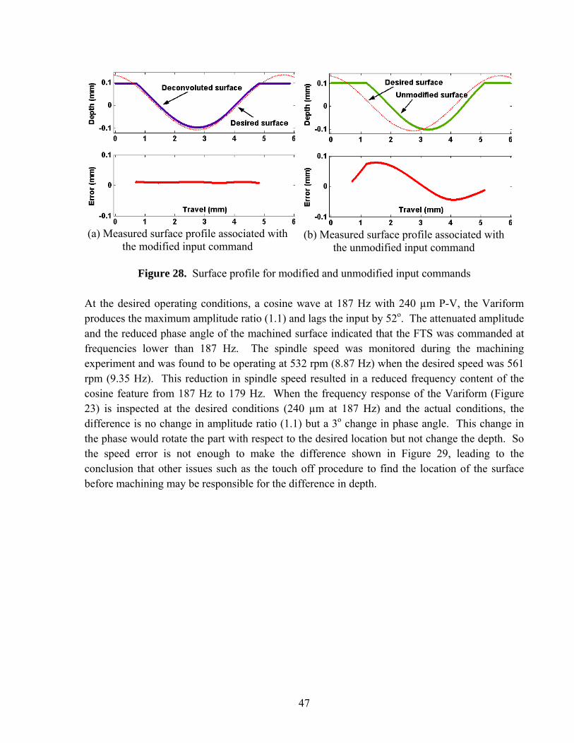
47

(a) Measured surface profile associated with the modified input command

(b) Measured surface profile associated with the unmodified input command

Figure 28. Surface profile for modified and unmodified input commands

At the desired operating conditions, a cosine wave at 187 Hz with 240 µm P-V, the Variform produces the maximum amplitude ratio (1.1) and lags the input by 52o. The attenuated amplitude and the reduced phase angle of the machined surface indicated that the FTS was commanded at frequencies lower than 187 Hz. The spindle speed was monitored during the machining experiment and was found to be operating at 532 rpm (8.87 Hz) when the desired speed was 561 rpm (9.35 Hz). This reduction in spindle speed resulted in a reduced frequency content of the cosine feature from 187 Hz to 179 Hz. When the frequency response of the Variform (Figure 23) is inspected at the desired conditions (240 µm at 187 Hz) and the actual conditions, the difference is no change in amplitude ratio (1.1) but a 3o change in phase angle. This change in the phase would rotate the part with respect to the desired location but not change the depth. So the speed error is not enough to make the difference shown in Figure 29, leading to the conclusion that other issues such as the touch off procedure to find the location of the surface before machining may be responsible for the difference in depth.

48

Figure 29. The deconvolved surface was offset by 10 µm with respect to the desired surface 2.4 CONCLUSION An input shaping technique using digital signal processing tools was evaluated to correct form errors caused by the dynamics of the Variform fast tool servo. The fundamental concepts of convolution are introduced in this report to explain the causes of attenuated and delayed excursion and to formulate a corrective algorithm. By applying deconvolution (the inverse dynamics algorithm) to a desired motion path, the dynamics of the actuator can be counteracted yielding a significant reduction in steady-state form errors. Not only is the magnitude of the error reduced by nearly two orders of magnitude, the analytical simulation predicts the experimental behavior very closely. The response shows practically no delay from the desired excursion after a startup interval lasting approximately 4 ms. In practice, this startup period will be designed to occur outside the machined region and will not affect the surface shape. Since the entire command signal needed to machine a surface can be generated a priori, the deconvolution is performed once for a given set of machining parameters (e.g., spindle speed, cross feed, tool radius). The technique critically depends on knowledge of the actuator impulse response and the proposed operating conditions. The deconvolution technique produces better form accuracy for machined surfaces than unmodified input commands. The bulk of the improvement is due to the phase compensation because the internal analog controller of the Variform does a good job of keeping the amplitude ratio equal to one over the range of frequencies from DC to 200 Hz. However, over that same range, the phase angle changes from 0 to 50º. Two surfaces were machined to demonstrate the effectiveness of this technique to correct form errors; an off axis sphere and a cosine wave shaped cavity. The off axis sphere had a depth of 120 µm, a radius of 12.33 mm, the center was 20 mm off the axis of rotation and the resulting

49

dimple was about 3 mm in diameter. The sphere was cut at 2 speeds (500 and 250 rpm) and the form error was ±2 and ±1 µm, respectively. The second surface was a cosine shaped feature cut at a depth of 240 µm. In this case, the spindle speed was about 550 rpm and the frequency command to the Variform was nearly 180 Hz, which is near its operating limit. The resulting surface had a form error of ±2 µm. The machining experiments corroborate the simulated results and the tool path measurements using the laser interferometer on the Variform mounted on an optical table. The figure errors can be decreased by two orders of magnitudes due to the significantly reduced phase response. However, even if a simple phase and gain adjustment on the output is made, it cannot eliminate the dynamic response of the FTS. This technique adds the subtle changes in the shape of the input command signal to yield an output tool path close to the desired excursion. The limitations of this technique appear with the combination of high frequencies and large amplitudes. Actuator motion is constrained by the maximum velocity of the electro-mechanical system resulting in an uncorrectable error. At frequencies above 340 Hz even a saturated input signal (±10 volts) will not produce a full magnitude tool excursion. These restrictions can be part of a procedure for automatically decomposing an arbitrary motion path into its constituent sinusoids and producing a modified command signal that drives an actuator to follow the desired profile. Inputs to this procedure will also include the actuator impulse response and the machining parameters.

REFERENCES 1. Smith, Steven W., “The Scientist and Engineer's Guide to Digital Signal Processing,” 2nd

Edition, California Technical Publishing, (1999). 2. Shannon, C.E. and W. Weaver. The Mathematical Theory of Communication. The

University of Illinois Press, Urbana, Illinois, (1949). 3. Tomizuka, M., “Zero phase error tracking algorithm for digital control,” ASME J. Dynam.

Syst. Meas., Contr., vol 109, pp. 65-68, (Mar 1987). 4. Yeh, S., and P. Hsu, “An optimal and adaptive design of the feedforward motion controller,”

IEEE/ASME Transaction. Mechatronics, vol 4, n 4, Dec 1999. 5. Kobayashi, H., Endo, S., Kobayashi, S., and C.J. Kempf, “Robust digital tracking controller

design for high-speed positioning system – A new design approach and implementation techniques,” International Workshop on Advanced Motion Control, AMC, v 1, 1996, p 65-70.

50

6. Cattell, J., M. Byl, and D. Trumper, “Adaptive feedforward cancellation viewed from an

oscillator amplitude control prespective,” Precision Engineering, 2003 7. Byl, M.F., J.A. Calzaretta, S.J. Ludwick and D.L. Trumper, “Tuning Controllers with

Multiple Adaptive Feed-forward Cancellation Resonators,” Proceedings of the 3rd EUSPEN International Conference, 2002.

8. Singhose, W.E., W.P. Seering and N.C. Singer, “The Effect of Input Shaping on Coordinate

Measuring Machine Repeatability,” Proceedings of the 1995 IFToMM World Congress on the Theory of Machines and Mechanisms. 1995.

9. Boe, F. and B. Hannaford. On-Line, “Improvement of Speed and Tracking Performance on

Repetitive Paths,” IEEE Transactions on Control System Technology, 1997. 10. Abramovitch, D.Y. Rejecting, “Rotational Disturbances on Small Disk Drives using

Rotational Accelerometers,” Proceedings of the 1996 IFAC World Congress, 1996. 11. Mitra, S.K., “Digital Signal Processing, A Computer-Based Approach, ” McGraw-Hill, 1998 12. Oppenheim, A.V. and R.W. Schafer, “Discrete-Time Signal Processing, ” Prentice Hall,

1998 13. Panusittikorn, W. “Error Compensation using Inverse Actuator Dynamics”, PhD

Dissertation, North Carolina State University, 2004.

51

3 TEM AND RAMAN SPECTROSCOPIC ANALYSIS OF HIGH PRESSURE PHASE TRANSFORMATIONS IN DIAMOND TURNED SINGLE CRYSTAL SILICON

Timothy Kennedy

Travis Randall Graduate Students

Ronald Scattergood Professor

Department of Materials Science and Engineering

Diamond cubic silicon (Si-I) is a brittle material under standard temperature and pressure, but when exposed to a high pressure environment, the crystal structure transforms into a ductile β-tin metallic phase (Si-II). Once the Si-II is unconstrained, it back transforms into multiple forms of Si, mainly amorphous Si (a-Si) and Si-I. This transformation allows silicon to be machined without brittle fracture occurring, but the back transformation alters the surface (~500 nm in depth). This alteration can be divided into two layers: an amorphous layer and a damage layer. The amorphous layer extends from the surface down as far as 200 nm; this is the a-Si byproduct of the back transformation process. Below the amorphous layer, a damage layer extends another 300 nm; this layer exists due to the stresses from the machining process and is comprised of dislocation structures. Dislocations can change the properties of Si-I, while a-Si has entirely different properties. In situ analysis of this transformation during the manufacturing process is impractical. Using transmission electron microscopy (TEM), specifically cross sectional TEM (XTEM) and Raman spectroscopy, a portrait can be formed to explain how and why Si-I transforms into Si-II and back into a-Si and Si-I.

52

3.1 INTRODUCTION This study is part of an NSF sponsored research program intended to examine the high pressure phase transformations of brittle materials (silicon, germanium, silicon nitride, etc) during manufacturing processes. Previous research in the PEC has focused on the affects of scribing on silicon [1]; this particular study is focused on diamond turning of single crystal silicon. When silicon is subjected to high pressures, it transforms from a brittle diamond cubic silicon (Si-I) to a metallic β-tin phase (Si-II); this transformation permits the ductile machining of normally brittle silicon. Once the pressure is released, the Si-II back transforms into a combination of different silicon phases, mainly amorphous silicon (a-Si) and Si-I. [2] The surface roughness of silicon after turning is comparable to that of traditional electrochemical polishing. [1] Even though reasonable surface roughness is obtainable, subsurface alteration occurs. An amorphous layer and a damage layer reside below the surface to a depth of 500 nm or more. The amorphous layer is a result of the back transformation process from Si-II and can be as thick as 200 nm. The damage layer sits right below the amorphous layer and consists of dislocation structures. If these layers can be controlled, then diamond turning of silicon wafers would be a more cost effective means of wafer preparation than electrochemical polishing. In situ observation of the high pressure phase transformation in silicon is nearly impossible during the machining process. The best way to theorize why and how the silicon transforms and back transforms is to use transmission electron microscopy (TEM) and Raman spectroscopy to observe the back transformed material. The only draw back to Raman spectroscopy is that quantitative data is hard to ascertain, compared to TEM, which provides excellent quantitative data. 3.2 DETAILS OF THE PROJECT For this project, TEM and Raman data will be collected from (100) oriented silicon that has been diamond turned along the <110> and <001> type directions. Different crystal orientations are available, but it has been shown that (100) oriented silicon provides the best ductility [1]. Machining parameters and techniques will also need to be examined. 3.2.1 EXPERIMENTAL SETUP A Rank Pneumo ASG 2500 Diamond Turning Machine (DTM) will be used to create the samples for this study. The samples used are 10 mm wide by 20 mm long, and are oriented so that the cutting direction follows either the <110> or <001> type directions across the 1 cm width. The tools being used are 3 mm radius round-nosed diamond tools with rake angles of -30° and -45°. Currently samples are prepared by fly cutting. This technique should increase the

53

life of the diamond tool because the diamond is not always in contact with the silicon. Because chemical wear is the dominant wear mechanism, the intermittent contact during fly cutting should reduce the wear. The parameters used during turning have an effect on the amount of back transformed a-Si. [3] The slower the feed rate, the more amorphous material is formed; so spindle speed and feed rate need to be optimized so that the layered structure can be controlled through machining, instead of other processes such as thermal annealing. It has also been shown that tool geometry has a great effect on subsurface layers. A straight nose tool produces the opposite that is observed with a round nose tool. [4] Samples have been prepared with feed rates of 15, 7, 5, 3, 2 and 1 µm/rev. Surface finishes of the ductile-turned regions were measured using a Zygo New View 5600 white light interferometer. MetroPro, the software suite used to analyze the interferometer data, reports a measure of surface roughness by the root mean square (RMS) parameter and peak to valley (PV) values. Measurements were taken from the center outward in regions within and outside the predicted fracture pattern area (further explained in Results section.) Once the surface finish is evaluated, samples are analyzed with Raman spectroscopy and TEM. 3.2.2 ANALYTICAL APPROACH Raman Spectroscopy Raman spectroscopy measures the intensity and wavelength of inelastically scattered light from molecules. The scattered light is shifted by the molecular vibrational energy, which is directly controlled by the interatomic bond length of the atoms in the sample [5]. In the case of silicon, each phase has its own interatomic bond length and thus, each phase would have a unique and sharp Raman spectrum. In the case of a-Si, the interatomic bond lengths vary, so the Raman spectrum from a-Si is broadened. Raman spectroscopy provides a view of what phases are present in the back transformed silicon and is able to detect these differences in vibrational energies to provide a qualitative view of phases present. TEM TEM is an electron microscopy technique that provides sub-nanometer resolution. Using a high energy electron beam (200kV), a detailed image is created. A method known as cross sectional TEM (XTEM) will be used since a planar view would not be able to illustrate the layered structure. Basic phase information can be gained through imaging, or electron diffraction, along with detailed dislocation information. The dislocation information cannot be directly seen using Raman spectroscopy.

54

3.2.3 EXPERIMENTAL RESULTS Optical quality, low RMS (1-10 nm) surfaces were created by diamond turning single crystal silicon wafers in the ductile regime. Ductile regime material removal was evident by the absence of fracture damage, repeated feed marks in the surface, and the generation of continuous chips. Increasing the feed rate created an increase in the surface roughness as shown in Figure 1; since increasing feed rate also reduces the amount of material removed by ductile processes.

Figure 1. RMS vs. Feed Rate for various feed rates on single crystal silicon. Feed rate seemed to be the limiting factor for generating a damage free surface. At increasing feed rates, certain directions on a wafer face initiated fracture before others, creating symmetric damage patterns on the surface. The more negative rake angle tool tended to suppress the onset of fracture in the favored direction, allowing machining at higher feed rates. The damage patterns for the wafer orientations tested ((100), and (111)) were very similar to those found previously and were explained qualitatively by an orientation stress model used in that research. [1] The pattern for (100) is shown in Figure 2.

55

Figure 2. Damage patterns for (100) wafer as a result of machining at sufficiently high feed rates.1

For surfaces that were ductile turned with similar parameters of tool rake and low feed rate, there appeared to be no difference in surface roughness and profile shape radially (changing cutting direction) as measured by interferometery methods. The RMS (and PV) value of ductile turned surfaces was limited by the effect of the condition of the tool. While tools were freshly sharpened, experimental preparation (i.e. part touch off and preliminary facing cuts) perhaps dulled the tips enough to result in non-ideal material removal (deformation under the tool and elastic spring back.) This was evident by higher-than-theorized PV values, and machining profiles that did not fit theoretical shape (but were similar to realistic expectations) as measured by interferometery techniques. Additionally, machining runs on silicon were subject to tool wear and damage considerations, as evident by the repeated patterns of tool damage features into the part surface. Despite these various problems, surfaces turned within the ductile regime had RMS values in the range of <1 nm to 10 nm increasing with feed rate. The characteristic Raman peak for Si-I is 520 cm-1, while a-Si has a lower peak at 470-1 due to its amorphous structure. As shown in Figure 3, the Si-I peak decreases as feed rate decrease, while the a-Si peak increases. The information on the far left of Figure 3 is background radiation. The intensity units are arbitrary on all Raman spectra. The downside of Raman is that quantitative data cannot be acquired. But a qualitative comparison is achievable by taking the ratio of heights of the Si-I and a-Si peak, as can be easily seen in Figure 4.

56

Figure 3. Raman spectra at feed rates a) 15, b) 7, c) 3, d) 2, and e) 1 µm/rev. [3]

Figure 4. Raman spectra from Figure 3 zoomed into 400-1-600-1, showing relative heights of peaks. [3]

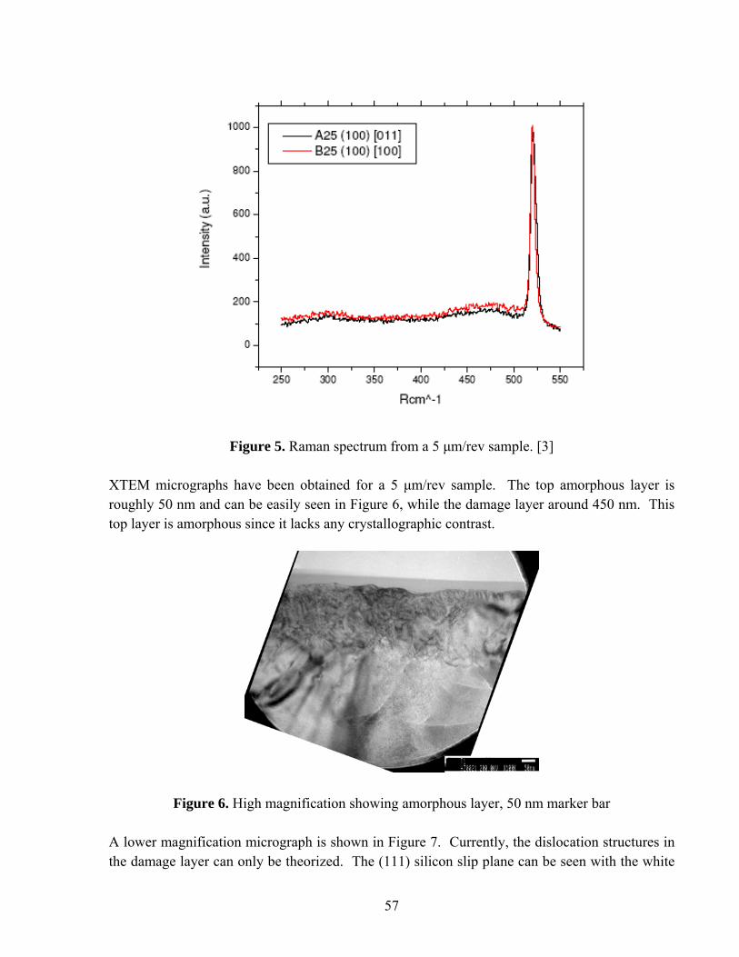
57

Figure 5. Raman spectrum from a 5 µm/rev sample. [3]

XTEM micrographs have been obtained for a 5 µm/rev sample. The top amorphous layer is roughly 50 nm and can be easily seen in Figure 6, while the damage layer around 450 nm. This top layer is amorphous since it lacks any crystallographic contrast.

Figure 6. High magnification showing amorphous layer, 50 nm marker bar

A lower magnification micrograph is shown in Figure 7. Currently, the dislocation structures in the damage layer can only be theorized. The (111) silicon slip plane can be seen with the white

58

line in Figure 7. The top plane is the (100) plane and an angle of 54° separates that with the (111) plane. This shows that some type of deformation process is occurring, but there is currently no reasonable explanation for it.

Figure 7. Low Magnification image showing depth of damage layer and slip plane 3.3 CONCLUSIONS Low RMS surfaces were achieved by ductile regime turning with high negative rake angles and large nose radius diamond tools for various crystallographic orientations of single crystal silicon. Symmetric fracture patterns resulting from high feed rate machining were the limiting factor for ductile regime machining. Surface characteristics, such as roughness and profile, seemed to show little dependence with respect to crystallographic orientation within the ductile regime. From the TEM and Raman data it is clear that the back transformed material contains an amorphous layer and a deeper damage layer. This structure has also been seen by other research groups, but it is important to note that nobody has taken an in depth look at this damage layer before. When the Raman spectra and TEM images are compared, the qualitative comparison is a good link between the two analytical techniques. Figure 5 shows a very small a-Si compared to its Si-I, this holds true when looking at Figure 7. There is a very thin amorphous layer compared to the rest of the image. Other things yet to be explained are the rectangular structures present at the bottom of the damage layer in Figure 7. Future Work More silicon samples need to be machined at different feed rates and with different machining techniques. These samples will then be examined with Raman and TEM. Atomic force microscopy (AFM) and scanning electron microscopy (SEM) will be explored as different methods of analyzing the silicon. New diamond tools have been purchased and will allow improved surface finishes, and the possibility of changing tool geometry will also be explored.

59

References 1. Randall, T., M.S. Thesis, Characterizing the Ductile Response of Brittle

Semiconductors to Dynamic Contact Processes, North Carolina State University, 2004. http://www.lib.ncsu.edu/theses/available/etd-06182004-104005/

2. Domnich, V. and Y. Gogotsi. “Phase Transformations in Silicon Under Contact

Loading”, Rev. Adv. Mater. Sci. 3(2002) 1-36 3. Walter, J., M.S. Thesis, Raman Scattering Analysis of Structural Transformations

Due Precision Engineered Si, 6H-SiC and β-Si3N4, North Carolina State University, 2004. http://www.lib.ncsu.edu/theses/available/etd-11302004-114015/

4. Yan, J. “Laser micro-Raman spectroscopy of single-point diamond machined

silicon substrates”. J. App. Phys. Vol. 94 Number 4 (2004) 2094-2101 5. http://elchem.kaist.ac.kr/vt/chem-ed/spec/vib/raman.htm

60

4 MICROMACHINING USING EVAM

Brett Brocato Graduate Student

Dave Brehl Graduate Student

Alex Sohn Precision Engineering Center Staff

Thomas Dow Professor

Department of Mechanical and Aerospace Engineering

The goal of this research is to demonstrate Elliptical Vibration Assisted Machining (EVAM) as a 3-D micro-structuring tool for MEMS applications. While many MEMS (MicroElectroMechanicalSystems) devices are fabricated using silicon etching techniques developed for the microelectronics industry, micro-machining is an attractive alternative because of its low start-up cost relative to other capital-intensive MEMS technologies. The Ultramill Elliptical Vibration Assisted Machining (EVAM) system has unique capabilities among micro-machining techniques. Its features include zero runout and a tunable vibrating tool path. Three-dimensional structures with 15 µm plan-view features, 500 nm elevation features, and 20 nm RMS surface finish have been achieved on a 200 µm part scale.

61

4.1 INTRODUCTION Microelectromechanical systems (MEMS) offer designers the ability to create miniature mechanical oscillators, optical network components and biological labs on a chip. Although manufacturers are introducing a wide range of MEMS-based products, developers have found that guiding MEMS devices from the laboratory to the marketplace is a costly and time-consuming venture. For example, it is not unusual for a single MEMS prototyping run to take 3 months. The high cost of a MEMS fabrication facility forces companies to use existing foundries such as Sandia, MCNC or Berkeley with long lead times. The problem lies not with the MEMS devices themselves, but with the semiconductor-based manufacturing techniques employed to build them. Semiconductor wafer fabs excel at producing high-volume integrated circuits using standard CMOS processing, but many MEMS devices are manufactured in lower volumes with more complex structures, such as moving three-dimensional micromirror arrays.

Technology / Feature Geometry

Min. Feature size** / Feature tolerance

Feature Positional Tolerance

Material Removal Rate

Materials

Focused Ion Beam/ /2D & 3D

200 nm / 20 nm 100 nm 0.5 µm3/sec Any

Micro Milling or Turning /2D or 3D

25 µm / 2 µm 3 µm 10,400 µm3/sec Polymers, Al, Brass, Nickel, SS and Titanium

Excimer Laser /2D or 3D

6 µm / < 1 µm < 1 µm 40,000 µm3/sec Polymers, Ceramics and some metals

Femto-Second Laser /2D or 3D

1 µm / <1µm < 1 µm 13,000 µm3/sec Any

Micro-EDM(Sinker or Wire) /2D or 3D

25 µm /3 µm 3 µm 25x106 µm3/sec Conductive materials

LIGA /2D

< 1 µm / 20-500 nm

~ 300 nm across 75 mm

N/A Copper, Nickel, Permalloy

Table 1. Material and Feature Size Guidelines by Process Type [1]

There are non-semiconductor processes for making MEMS devices that include focused ion beam machining, mechanical turning and milling, laser processing, electro-discharge machining

62

and LIGA. Each technique can be classified in terms of minimum feature size, position tolerance, maximum material removal rate and material compatibility [1] as shown in Table 1. Focused Ion Beam (FIB) machining is a process in which the kinetic energy of accelerated ions is converted to thermal energy and used to vaporize very small amounts of material from a workpiece. It is a 3-D process with extremely high tolerances that can be used on any material. The main disadvantages are slow material removal rate (MRR) and high equipment costs. Excimer lasers and femto-second lasers have comparable removal rates to micro-machining. The achieved tolerances are superior to micro-machining. Excimer lasers have less material flexibility than micro-machining. Micro-Electro Discharge Machining (Micro-EDM) has an extremely high MRR and comparable accuracy to micro-machining, but only works on conductive materials. The most common material-removal processes in macro manufacturing are turning and milling. The lower dimensional limits of these processes are being expanded by current research. Micro-machining is the process of chip removal by means of a spindle and an end mill in the diameter range of 200-µm or less. Part features are on the order of 25 µm. Carbide milling tools are commercially available in 100-µm size. Researchers have created custom diamond tools as small as 22 µm. Feature aspect ratios of 40:1 have been achieved on machined parts. Micro-machining has the advantage of greater material and geometry flexibility than that of lithography and most other micromachining processes. Current micro-machining techniques using a high-speed spindle are plagued with tool runout that limits the feature size and tolerance. A proposed concept is to replace the high-speed spindle with a piezoelectrically driven tool holder that can move the diamond tool tip in an elliptical motion at frequencies up to 5000 Hz - the equivalent of 300,000 rpm. The two actuators are driven independently to create a tool path that can be changed from linear to elliptical to circular with the amplitude, frequency and phase of the excitation voltages. Advantages of this technology include:

• Optical surface finish • Sub-micrometer 3D feature size and position • Extremely low cutting forces • No burring at the edge of a cut • Applicable to a wide range of materials – metals, plastics and ceramics

A terminology convention will be used throughout this report to differentiate between the vibrating motion of the Ultramill diamond tool and the overall motion of the Ultramill as a unit during machining operations. The Ultramill’s diamond tool motion with respect to the Ultramill body will be referred to as the tool path. The motion of the Ultramill body with respect to the

63

workpiece will be referred to as a motion plan or motion program. Two states of repair for the Nanoform 600 DTM y-axis will be discussed in this paper. State “A” is a condition of degraded air bearing stiffness. State “B” is the nominal condition of the axis. 4.2 EXPERIMENTAL APPARATUS 4.2.1 ULTRAMILL ELLIPTICAL TOOL PATH The Ultramill linkage consists of two piezoelectric actuators with pin connections to the tool holder and diamond tool. The elliptical tool path is generated by actuating the piezo stacks with out-of-phase sinusoidal voltage signals. An illustration of the tool path is shown in Figure 1.

� � � � � � � � �

�

�

��

� �

��

� � � � � � � � �

0 45 90 135 180 225 270 315 360

�� ����

������������������

������������������

����

��

���

����

��

���

Figure 1. Ultramill tool path.

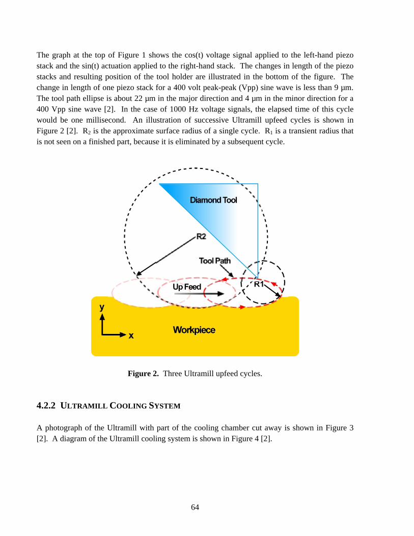
64

The graph at the top of Figure 1 shows the cos(t) voltage signal applied to the left-hand piezo stack and the sin(t) actuation applied to the right-hand stack. The changes in length of the piezo stacks and resulting position of the tool holder are illustrated in the bottom of the figure. The change in length of one piezo stack for a 400 volt peak-peak (Vpp) sine wave is less than 9 µm. The tool path ellipse is about 22 µm in the major direction and 4 µm in the minor direction for a 400 Vpp sine wave [2]. In the case of 1000 Hz voltage signals, the elapsed time of this cycle would be one millisecond. An illustration of successive Ultramill upfeed cycles is shown in Figure 2 [2]. R2 is the approximate surface radius of a single cycle. R1 is a transient radius that is not seen on a finished part, because it is eliminated by a subsequent cycle.

Figure 2. Three Ultramill upfeed cycles. 4.2.2 ULTRAMILL COOLING SYSTEM A photograph of the Ultramill with part of the cooling chamber cut away is shown in Figure 3 [2]. A diagram of the Ultramill cooling system is shown in Figure 4 [2].

65

Figure 3. Ultramill cut-away.

Figure 4. Ultramill cooling system.

The reservoir, chiller, pump, and controller are contained within a Thermocube thermoelectric cooler. The controller maintains a constant temperature of the fluid returning to the reservoir from the Ultramill cooling chamber. This temperature is the setpoint of the Thermocube controller. The fluid used is 3M Fluoroinert 3283. It is a dielectric, extremely low viscosity coolant chosen to be compatible with the piezoceramic actuators and to promote turbulent

66

convection [2]. The Thermocube is equipped with a 30 Hz diaphragm pump. Transmission of pump vibration to the Ultramill was minimized by using gravity flow through the cooling chamber and separating the inlet hose from the chamber. 4.2.3 NANOFORM/ULTRAMILL INTEGRATION The Ultramill was adapted to the 3-D micro-structuring application by mounting it on the Nanoform 600 3-axis DTM. This allows the Ultramill to be moved in x- and z-directions with 1.25 nanometer resolution, and in the y-direction with 40 nm resolution. Figure 5 shows the experimental assembly.

Figure 5. Experimental Setup.

The Ultramill is mounted on the y-axis. Figure 5 also shows the 130x video microscope used for Ultramill touch-off and process monitoring. The parts to be machined are placed on the Nanoform vacuum chuck. The inset shows the rake face of the 1 mm radius Ultramill diamond tool and a side view of the static diamond tool used to turn parts flat before machining. A blank is placed on the vacuum chuck and diamond-turned to the desired surface finish before the Ultramill is used. After a blank is prepared with the static diamond tool, the vacuum chuck and spindle are locked to prevent rotation in preparation for micromachining using the Ultramill. In the inset of Figure 5, the major axis (a) of Ultramill tool motion is in the x-direction and the minor axis (b) is in the z-direction. Upfeed of the Ultramill is accomplished by Nanoform x-axis motion, which in turn moves the vacuum chuck and part with relation to the Ultramill. Vertical

67

motion of the y-axis is the crossfeed direction for the Ultramill. Touch-off and depth of cut changes for the Ultramill are controlled by the z-axis. 4.2.4 MICROMACHINING EXPERIMENTS Micromachining is accomplished by rastering the Ultramill across the face of the part. Figure 6 shows an example machining sequence of five raster passes for a flat with no depth changes.

Figure 6. Rastering sequence. In this example, the upfeed distance is 2 mm and the crossfeed increment is 1 µm per pass. Negative-x direction on the Nanoform 600 is the upfeed direction for the Ultramill. At touch-off, the z-axis is zeroed at the apparent surface of the part. In the Nanoform coordinate system, negative-z displacements from zero are deeper into the part. Figure 6 shows five raster passes with a 3 µm intended depth of cut and a 1.5 µm clearance from the part during x-axis backfeed. 4.3 ULTRAMILL MOTION PLANNING Traditional micro-milling motion programs require that the tool center path be offset from the desired surface by the fixed tool radius. The elliptical motion of the Ultramill diamond tool means that the effective tool shape changes with the relative orientation of the Ultramill and the desired structure. This section will discuss how Ultramilled surface features affect the motion program path, graphical methods of Ultramill motion planning, and proposed methods of automatic motion program generation.

68

4.3.1 ULTRAMILLED SURFACE FEATURES Surface finish of a raster-cut flat surface is affected by Ultramill actuation frequency, elliptical tool path, tool radius, upfeed speed and crossfeed pass increment. The peak-to-valley (PV) surface finish in the upfeed direction is approximated by Equation 1 [2].

)(8 2

2

RufpcPV = (1)

In Equation 1, ufpc is the upfeed per cycle, defined as the upfeed velocity divided by the

Ultramill actuation frequency. R2 in Equation 1 is the surface radius of the workpiece at the

bottom of the Ultramill tool path. It is approximated by Equation 2 [2]

baR

2

2 = (2)

In Equation 2, a is the major axis of the Ultramill tool path ellipse and b is the minor axis. PV surface finish in the crossfeed direction is defined by Equation 3 [2].

)(8

2

tRfPV = (3)

In this expression, Rt is the tool radius and f is the crossfeed increment per pass. Micro-structured features on Ultramilled parts depend on elliptical tool path size, tool radius, feed speed, or increment of the Nanoform axes, and depth of cut. A typical negative surface feature created by a plunge into the part may be described by the terms depth of cut (DOC), width of cut (WOC), and length of cut (LOC). Width of cut is equal to the chord of the tool radius at a given depth of cut and is illustrated in Figure 7.

Figure 7. Width of Cut

69

Length of Cut (LOC) is equal to the chord of the tool motion ellipse at the depth of cut. It is illustrated in Figure 8.

Figure 8. Length of Cut.

Length of cut may be calculated using Equation 4.

(4)

The relationship between DOC, WOC and LOC for the tool radii used in this research is shown in Figure 9.

Figure 9. DOC vs. WOC and LOC.

:= LOC2 − 2 b DOC DOC2 a

b

70

This minimum negative surface feature must be taken into account when programming Ultramill tool motion to produce a 3-D micro-structure. If a feature is to remain on the part, the Ultramill tool path center may approach it no closer than LOC / 2 in the upfeed direction or WOC / 2 in the crossfeed direction during the machining process. 4.3.2 MOTION PLANNING An Ultramill motion program path must be planned using varying approach distances between the tool path center and a desired structure. These approach distances depend on the relative orientation of the Ultramill tool with respect to the micro-structure. If part features are orthogonal to the tool rake face and to the elliptical tool path major and minor dimensions, raised features may be preserved by limiting the motion program approach distance to either LOC/2 in the upfeed direction or WOC/2 in the crossfeed direction. Desired features not parallel to either feed direction require graphical planning of the motion program approach distance. This requirement is illustrated in Figure 10. The drawing shows a section of a 1mm x 1mm angstrom symbol with Ultramill negative features placed at critical points in the machining process.

Figure 10. Ultramill features. The angstrom symbol, the logo of the Precision Engineering Center, was used as a proof-of-concept micro-structure design for Ultramill motion planning. The 1 mm angstrom symbol was designed to be machined with the 1 mm radius Ultramill diamond tool. In this example, the design change in depth of cut from background to foreground is 500 nm. At that change in DOC, and with ellipse parameters a = 11 µm and b = 2 µm, the negative feature cut by the Ultramill is an ellipse 63 µm wide in the crossfeed direction by 14 µm long in the upfeed direction. If a raised feature is to be preserved, tool motion must be offset so that the raised feature has no interference with the Ultramill elliptical tool path. In the case of the diagonal

71

sides of the A, that amount is equal to the distance from the ellipse centroid to the ellipse’s point of tangency with the diagonal feature. The graphical method of Ultramill motion planning is complex and time-consuming. The angstrom symbol motion program required approximately 20 hours to write. The difficulty of this task is due to three factors: tool offset, raster pass development, and program length. The changing tool offset for the Ultramill with x-y orientation and z depth of cut change has already been discussed. Figure 10 shows a complex-geometry part with tool offsets. Writing a motion program to produce an arbitrary structure involves several steps. For all points on each raster machining pass, the entire perimeter of the offset clearance ellipse must be checked to make sure it neither encroaches on features raised above the cutting plane, nor misses locations where cuts are desired. This takes excessive time when performed manually. Raster machining requires determining the X and Y coordinates where the tool must execute Z direction motions (lift from or plunge into the part). This must be done for each change in elevation for features on the part, and for every raster pass. Parts machined to date have required from 50 to 200 raster passes. The PMAC controller used on the Nanoform 600 uses a low-level language. The commands are simple but many are required to execute a sequence of tool moves. Programs to machine typical contoured parts are estimated to need from of 600 to 3500 commands. Writing the program therefore is laborious, slow, and prone to typing and logic errors. To more readily create Nanoform machining programs, an effort was begun to automate the processes for motion program planning and PMAC code writing. This has resulted in two MATLAB programs for machining program generation. The first program, MORPH3, finds the tool-offset points required to produce a given feature edge, and calculates the X and Y coordinates at which tool motions in Z (lift or plunge) must be executed. At present, the program is limited to part designs with only 2 levels in the vertical or Z direction, i.e. raised features on a machined background. Also, the edges of the raised features must be perpendicular relative to the machined background. The second program, PMACWRITER, generates code for a machining program, in a standardized format. Although some editing is usually necessary before the machining program can be used, nearly all of the routine labor has been eliminated. The required offsets for the tool center point can be determined using the morphological operation of “dilation” [3]. Dilation is a mathematic operation analogous to “touching” a “probe” of known geometry to an unknown surface (Figure 11). An image is constructed by observing the displacement of the probe relative to a reference point, as it is swept along the surface locations with the probe. In the situation here, the “probe” is the offset ellipse for the tool center, and the “surface” is the set of edges defining raised features on the part. The

72

coordinates of the points defining the dilated image correspond to the X and Y locations of the tool center point, where Z motion (lift or plunge) must occur, to produce the desired features.

Figure 11. Dilation of a Surface.

“Erosion” is an operation, which applies a known probe to a dilated image, to reconstruct the surface. Generally the reconstruction deviates from the actual surface, since variations in the surface result in contact at different points on the probe. For Ultramill machining, the eroded surface may be thought of as the part, which will actually be produced, given the required tool center offsets. Features cannot be produced if they are of smaller scale than the tool center offset ellipse. This will be illustrated below. MATLAB’s Image Processing Toolbox contains standard functions to perform dilation (imdilate) and erosion (imerode) on an array of data. In this case, the data array is a discretized representation (bit map) of the part to be machined. The elliptical probe (called a “structural element” in the MATLAB functions) is approximated by a rectangle with dimensions equal to the major and minor axes of the tool center offset ellipse. The first step in developing a machining program is to create a bit map of the part. This can be done by scanning a black and white image, or by manipulating a CAD drawing made in a program such as Solidworks, as in Figure 12, left. In this initial bit map, the raised sections of the part are dark, while the background is light. The bit map must be scaled, so that each pixel in the crossfeed direction corresponds to the planned crossfeed increment for machining (i.e., if the crossfeed increment is to be 2 µm per pass, then each pixel has a crossfeed dimension of 2 µm). Pixel scale in the upfeed direction is arbitrary, although square pixels are typical.

73

Figure 12. Solidworks model of sample part (left), scaled bitmap (right). The MATLAB program MORPH3 is then run, using this scaled bitmap (Figure 12, right) and dimensional information for the tool center offset ellipse. MORPH3 creates a rectangular structural element that approximates the clearance ellipse, which is used in the dilation and erosion functions. Output from the program consists of a repeat of the bit map of the original part (Figure 13, left); the dilation (Figure 13, middle); the erosion of the dilated image (Figure 13, right); and a tabular listing of the tool motions in Z by pass, X (upfeed) and Y (crossfeed) coordinates. The MATLAB image processing functions require a reversal of the scheme used to indicate surface height on the part—in Figure 13 note that black now represents the background, and white indicates the raised portions of the part.

74

Figure 13. Sample part from Figure 12 showing original bitmap (left), dilation (middle), erosion from dilation (right)

The reconstructed surface, obtained by eroding the dilated image, is useful in checking that the machined part will actually be as designed. Figure 13 used a tool center offset ellipse consistent with the scale of the features on the part. In Figures 14 (left) and 14 (right), the offset ellipse is oversized relative to the smallest features on the part. Figure 14 (right) clearly shows that the finished part will have unintended features. In this case it will be necessary either to modify the design of the part, change tool geometry, or adjust the dimensions of the machining ellipse.

75

Figure 14. Dilation (left), erosion of dilated image (right) with oversize offset ellipse

The motion program coordinates determined by the MORPH3 program are used as input to the PMACWRITER program, which generates the actual text file used by the Nanoform’s PMAC controller. PMACWRITER consists of standard text blocks of PMAC commands, into which are inserted the numerical values calculated by MORPH3 for a specific part design. Three sources of possible deviations between the actual vs design parts have been identified. The first type, depicted in Figures 14 (left) and 14 (right), comes from a mismatch between the resolution needed on the part and the size of the tool center offset ellipse. A second problem stems from using a rectangular probe for dilation and erosion, instead of the actual ellipse. Using an array of pixels, which more closely approaches the shape of the tool center offset ellipse, can reduce this error. A third error source results from using a bit map instead of an analytical model—curves and diagonals are depicted as series of stepped squares, instead of in their true shape. But raster machining itself is inherently a discrete operation, since cross feed passes are made at specified intervals. The estimated error in feature size, arising from this source, is from ½ to 1 ½ times the pixel dimension, depending on the orientation of the feature edge relative to the tool path. Most of the parts machined to date have used a crossfeed step of 1 µm per pass. Had these parts been machined using a program generated from a bit map, the pixel size would be 1 µm square, and there would be a potential error of approximately 1.5 µm from the original design drawing.

76

4.3.3 MICROMACHINING RESULTS Two sizes of 3-dimensional structures were manufactured. The first was made with the 1 mm-radius Ultramill diamond tool. It was a 1 mm-square version of the Precision Engineering Center angstrom logo. The second, made with the 50 µm-radius tool, was a 200 µm-square version of the logo. The comparative size of the structures is shown in Figure 15.

Figure 15. Interferograms of 1 mm angstrom symbol and 200 um angstrom symbol (top left). The workpiece material for all machining experiments in this report is hard-plated copper. The 1 mm-square angstrom symbol shown in Figure 15 was made with the rastering sequence similar to the one shown in Figure 6 of section 4.2.4. Upfeed and crossfeed directions are shown for reference in Figure 15. Figure 16 shows a background upfeed direction profile of this part with the location of the profile highlighted on a partial view of the part.

Figure 16. 1 mm angstrom background upfeed profile: 159 nm PV, 32 nm RMS.

77

Due to a programmed upfeed speed incompatible with the acceleration limits on the Nanoform 600 control system, upfeed speed was not constant at any point on this part. The average upfeed speed was approximately 2.4 mm/sec. At 1000 Hz Ultramill actuation frequency, the approximate ufpc is 2.4 µm upfeed per cycle. Theoretical PV error in the upfeed direction is about 12 nm. The PV error over this profile is 160 nm. Surface frequencies lower than 416/mm (1000 Hz at 2.4 mm/s) are visible. A crossfeed profile of this part is shown in Figure 17.

Figure 17. Angstrom background crossfeed profile: 119 nm PV, 26 nm RMS.

The crossfeed increment between passes was 5 µm. With the 1 mm radius tool, this gives a theoretical crossfeed PV error of about 3.1 nm. PV error over this profile is 119 nm. Over the 300-µm length of the inspection profile, 60 crossfeed cycles were expected. The lower-frequency visible peaks in this area indicate unknown variables in the process. Due to surface errors greater than 100 nm peak-peak in the parts shown above, the authors investigated the performance of the y-axis air bearing. After adjusting the y-axis to increase the stiffness by 100% (nominal state B), a 200 µm x 200 µm angstrom symbol was machined using the 50 µm radius tool. Figure 18 shows a background upfeed profile of this part, and Figure 19 shows a background crossfeed profile. Upfeed speed for this section of the angstrom averaged 0.5 mm/sec. The part was machined with the Ultramill running at 1000 Hz. The ufpc is 500 µm at that speed. The theoretical PV error in the upfeed direction is about 1 nm. The PV error in this upfeed profile is 40 nm. The area of interest in Figure 19 is masked so that the raised sections of the angstrom symbol will not dominate the Zygo NewView’s best-fit-plane calculation. The crossfeed increment for this part was 1 µm. The theoretical PV error in the crossfeed direction with the 50 µm radius tool is 2.5 nm. Over the 85 µm length of this profile, there should be 85 crossfeed marks of 2.5 nm height. The PV error in this profile is 91 nm, and the RMS error is 19 nm. Figure 20 shows the smallest feature

78

achieved with the Ultramill to date. This section of the symbol is 15 µm wide in the upfeed direction.

Figure 18. 200 µm angstrom symbol background upfeed: 40 nm PV, 10 nm RMS.

Figure 19. 200 µm angstrom symbol background crossfeed: 91 nm PV, 19 nm RMS.

79

Figure 20. Angstrom symbol feature detail: 15 µm upfeed dimension.

Rastered flats were machined with the Ultramill to assess best-case form and finish capability. Because no depth of cut change is required during an upfeed pass, upfeed speed is constant over a significant portion of the part. Constant surface frequencies in the upfeed direction allow comparison of significant frequencies in the machining process with those on the part. The part in Figures 21 and 22 was machined with the y-axis in its nominal state B and with the 50 µm-radius Ultramill tool. The upfeed speed was 100 mm/min upfeed speed and the crossfeed increment was 1.67 µm. At 1000 Hz, the upfeed speed of 1.67 mm / sec yields a 1.67 µm upfeed per cycle (ufpc). An upfeed profile at 100x is shown in Figure 21. Over the 16.7 µm length of the profile, the 10 expected Ultramill cycles are visible. The expected PV height of these cycles is 6 nm. Each peak shown is about 10 nm above the local mean of the profile. A longer profile is shown in Figure 22. The 30 Ultramill cycles expected in this 52 µm profile are visible in this figure, but 3 lower-frequency waves are also visible, with a spatial frequency of about 58/mm. At the programmed upfeed speed of 1.67 mm/s, this translates to a time-domain frequency of 97 Hz. Frequencies in this range are supported by z-axis position data and capacitance gage vibration data discussed in the next section.

Figure 21. Upfeed profile showing 10 Ultramill cycles at 1.67 µm per cycle.

80

Figure 22. Upfeed profile: low frequency, 1.67 mm/s upfeed. 4.4 DISCUSSION OF SURFACE FEATURES 4.4.1 ULTRAMILL VIBRATION 4.4.1.1 Y- and Z- axis Combined Some of the experiments were performed with the y-axis in a state of degraded stiffness, referred to as State A. Measurements of vibration with the Ultramill running were taken before and after the air-bearing repair. A capacitance gage was mounted on the Nanoform x-axis targeting the forward face of the Ultramill beside the tool holder. Because the y-axis is mounted on the z-axis, data acquired with this experiment includes both z-axis motion and y-axis air-bearing vibration. The peak-peak vibration with the y-axis in its degraded state A is about 230 nm. The dominant frequency of vibration in this state is the 1000 Hz UMHS actuation frequency. Due to the high level of vibration, the y-axis air bearing was regapped to the design dimension. This configuration is known as state B. Figure 23 shows 25 kHz vibration data gathered after this procedure, and Figure 24 shows an FFT of that data. The peak-peak vibration is about 80 nm in this case. In the FFT, the 30 Hz amplitude peak of the diaphragm pump is visible. The largest amplitude in this data occurs at 10 Hz.

81

Figure 23. Cap gage output of State B: z-axis holding position, Ultramill 1000 Hz / 400Vpp

Figure 24. FFT of State B vibration. 4.4.1.2 Y-axis Vibration measurements were taken for nominal state B of the y-axis with the Ultramill mounted on the y-axis, but with the y-axis removed from the Nanoform. The vibration data is shown in Figure 25.

82

Figure 25. Y-axis state B vibration, mounted on optical table, Ultramill 1000Hz / 400 Vpp. The peak-peak vibration is about 80 nm. The 1000 Hz actuation frequency of the Ultramill is readily apparent in this signal. Figure 26 shows the low-frequency range of an FFT of this vibration data.

Figure 26. FFT of state B off Nanoform.

The largest peak in this low-frequency range is at 60 Hz.

83

4.4.1.3 Z-axis High-frequency axes position data has been gathered from the Nanoform 600 PMAC controller during the Ultramill experiments. Figure 27 shows 450 Hz data of ten consecutive passes in a rastered flat program with 2 mm upfeed distance and 1.5 µm crossfeed increment. The Ultramill was operating at 1000 Hz during this data collection. The data was gathered as a flat was being cut. A peak-peak position error of 19 nm occurs during the first pass at the bottom of Figure 27.

Figure 27. Ten 1.5 µm crossfeed passes (Ultramill actuated at 400 Vpp / 1000 Hz)

Figure 28. FFT of pass #1 An FFT of time-domain data from pass #1 is shown in Figure 28. The highest amplitude is at 13 Hz. This frequency shows some agreement with the 10 Hz peak observed in combined y- and z-

84

axes vibration in Figure 23. The programmed upfeed speed of this part program was 1.5 mm/sec. Position data from the x-axis was differentiated to yield data on upfeed speed and confirmed that the part speed within the central 1.8 mm in the x-direction was constant at 1.5 ± .05 mm/s. Surface frequencies in the upfeed direction should also be constant over this area. The 13 Hz peak of z-axis vibration (shown in Figure 28) should yield a spatial frequency of 19.5/mm at 1.5 mm/s. A 20x Zygo NewView white light interferogram of this flat was taken, covering 700 µm of upfeed distance in the center of the flat. Figure 29 shows a power spectral density (PSD) plot of an upfeed pass. The power spectral density plot shows a peak at 20/mm spatial frequency. This agrees with the 13 Hz peak in z-axis vibration shown in Figure 28. The lowest-frequency peaks in this PSD plot have a wavelength are on the order of the total size of the interferogram and should be neglected. The peak at 65/mm spatial frequency (97 Hz @ 1.5 mm/s) agrees with the 100 Hz peak in z-axis vibration shown in Figure 28.

Figure 29. Power spectral density, 1.5 mm/s upfeed pass. 4.4.2 TEMPERATURE EXPERIMENTS Because the motion commands of an Ultramill motion program are open loop, any change in operating condition will influence the position of the tool. One area of concern is the temperature, especially since the cooling system is needed to protect the piezoelectric actuators from damage. An experiment was performed to study thermal effects on Ultramill depth of cut. A flat 2 mm in the x (upfeed) direction by 200 µm in the y (crossfeed) direction was machined. The crossfeed increment used was 1 µm. A deliberate temperature excursion was caused just after pass 50. This was accomplished by raising the Thermocube controller’s setpoint temperature 5º C. This setpoint is the return temperature of the cooling system or the temperature of the Ultramill cooling chamber. The setpoint temperature was lowered to the original value (20º C) after reaching apparent thermal equilibrium at the elevated temperature. The 50 µm section of thermal equilibrium provided a baseline against which to measure the effects of the temperature excursion. The flat area also provided a rough fiducial feature to line

85

up (in y) the section of best-case flatness with the section of best-case temperature control. Depth of cut data was measured using the Form Talysurf profilometer.

Figure 30. Surface profile shown with theoretical thermal expansion. The surface profile is plotted as a function of crossfeed distance in Figure 30. The depth of the 50-um EVAM flat section between y = 0 mm and y = 0.05 mm is zeroed so that any deviations are equal to the change in depth of cut. A temperature excursion of 7º C in piezo stack skin temperature resulted in a change in depth of cut of 2.2 µm. These changes in temperature and DOC, when applied to the 24.4 mm length of the piezo stacks, indicate an effective coefficient of thermal expansion (CTE) of 13 ppm / ºC. The theoretical thermal expansion trace applies this CTE to the piezo stack temperature data. It is not obvious from these experimental results whether the temperature(s) controlling expansion had reached equilibrium at the time that the setpoint temperature was reduced, about five minutes after the initiation of the temperature excursion. Also, the slope of thermal contraction was neither constant nor equal to the slope of expansion. Due to the questions raised by these results, experiments were performed to directly measure tool holder position over longer periods of time. These experiments were performed with the Ultramill dismounted from the Nanoform 600. A light acrylic mounting block with a thin brass capacitance gage target was mounted on the Ultramill tool holder. The capacitance gage was positioned to measure average tool holder position. Federal gages were used to measure movement of the locknut face. Any deformation of the cooling chamber would be reflected by locknut motion. Figure 31 shows the experimental arrangement.

86

Figure 31. Capacitance and federal gages positioned to measure thermal expansion The piezo stack skin temperature, tool holder average total deflection, and Federal gauge deflections for 2 locations on the tool holder locknut are plotted as functions of time in minutes. Before each test, the Ultramill was allowed to come to thermal equilibrium after power was applied to the piezo stacks, as defined by no variation in either piezo stack temperature or coolant return temperature for at least 5 minutes. The control setpoint for the coolant return temperature was then increased by 3 degrees C in a single step. The coolant return setpoint was held constant for a period of 10 to 25 minutes, until the tool holder displacement appeared to have reached steady state. Then the coolant temperature setpoint was reduced by 3 degrees C to return to the original value. Data logging continued until it appeared that tool holder displacement had reached steady state. During the tests, the capacitance gauge measured instantaneous position data for the tool holder total deflection. This instantaneous data included the elliptical motion of the tool driven by the piezo stacks. The overall trend of the tool holder position envelope was watched visually to estimate when steady state deflection had been reached. The average position was determined by filtering the instantaneous data to remove the components of tool motion.

87

Figure 32. 3 degree temperature excursion, 25 minutes duration.

The tool holder average deflection, as a function of piezo stack temperature, is significant. Based on the upper equilibrium temperature of the piezo stacks (ignoring the overshoot right after changing the coolant return temperature), the tool holder expansion rate averages 0.8 µm / °C. If a similar rate holds for small piezo stack temperature changes, then even a 0.1 °C increase in stack temperature during machining could mean a growth in the tool tip position on the order of 80 nm, which could be a significant dimensional error for some machined parts. The tool holder average position change, as a function of piezo stack skin temperature, is not constant. While Figure 32 shows a maximum expansion of about 2.5 µm for a 3 ºC excursion, other test results ranged from 1.8 to 3.2 µm for similar conditions. It can take different amounts of time (from the time the coolant return temperature setpoint is changed) to achieve maximum tool holder expansion. The thermal deflection of the Ultramill cooling chamber is small compared to that of the tool holder, as shown by the Federal gage results. During a typical machining run, piezo stack temperature variation rarely exceeds 0.2 °C. The temperature excursions seen in these tests are extreme compared to operational situations. However, the relatively large piezo stack and/or tool holder expansions, which occurred during the test, indicate that temperature changes could be a major factor in Z-direction deviations from nominal depth of cut.

88

4.4.3 FUTURE WORK Future work in process characterization involves new analysis techniques for use with white light interferometer surface topology data and improved data gathering techniques for use during the machining process. Programs have been developed in Matlab for the analysis of specific surface features such as a single upfeed groove or crossfeed tool-radius feature. Nanoform axis-position data gathering techniques are being modified to produce higher-density data during the machining process that may be combined with part topology data to identify the causes of deviations from theoretical surfaces. Future work in automated program generation should address the following 3 items, most likely in the order presented: 1. Replacement of the rectangular “probe” used for dilation and erosion, with pixel arrays, which more closely approximate the shape of the tool, center offset ellipse. 2. Expanded capability of automatically generated machining programs to allow part designs with features located at several elevations above the background. 3. Extension of automatically generated machining programs to allow part designs with profiled edges, e.g. ramped or curved transitions between different elevations. 4.5 CONCLUSIONS Machining tests to date in hard-plated copper have demonstrated that EVAM using the Ultramill High Speed and Nanoform 600 combination is capable of sub-millimeter 3-D microstructuring. Microstructures as small as 200 µm square have been fabricated, comprised of binary features with arbitrary geometry as small as 15 µm wide and 0.5 µm high. Surface finishes of 14 nm RMS (40 nm PV) in the upfeed direction and 19 nm RMS (91 nm PV) in the crossfeed direction have been achieved. Tool geometry and motion programming are important factors in the scale and shape of 3-D features which can be achieved on a microstructure. Reducing the diamond tool’s nose radius from 1 mm to 50 µm allowed the overall size of a demonstration microstructure (the PEC’s angstrom logo) to be reduced from 1 mm to 0.2 mm square. Further work in motion program planning and machining strategy is expected to permit more complex (non-binary) 3-D geometries to be achieved, and may permit further reduction in feature sizes. Automated motion program generation will facilitate this work, by reducing the turnaround time required to run experiments.

89

Theoretical surface finishes in both the upfeed and crossfeed directions are less than 10 nm PV, as predicted by the EVAM tool path parameters. This is considerably better than results to date. Temperature excursions in the piezo stacks, DTM axes vibration, and electrical / controls issues all are potential reasons why theoretical finishes have not yet been achieved. Further work is required to identify the contribution of each of these factors to the machined surfaces, as well as which of them can be economically improved and by what degree. REFERENCES 1. Benevides, G., “Meso-machining Capabilities”, M4: Workshop on Micro/Meso-Mechanical

Manufacturing, Evanston, IL, May 2000. 2. Schaller, T, Heckele, M, Ruprecht, R, “Mechanical Micromachining for Mold Insert

Fabrication and Replication”, ASPE Proceedings, Vol.19, Pg 3-8, 1999. 3. Negishi, N, “Elliptical Vibration Assisted Machining with Single Crystal Diamond Tools”,

MS Thesis, NC State University, 2003. 4. Villarrubia, J.S., Journal of Research of the National Institute of Standards and Technology,

4, 102 (1997)

90

5 LIVE-AXIS TURNING

Nathan Buescher Graduate Student

Alex Sohn Research Assistant, Precision Engineering Center

Thomas A. Dow Professor

Department of Mechanical and Aerospace Engineering

The term Live-Axis turning (LAT) has been coined to describe a lightweight, linear-motor driven, air bearing slide that can be used to fabricate non-rotationally symmetric optical components. The system described is the result of a joint effort by the PEC and Precitech to create a long-range fast tool servo to fabricate future NASA optics. The slide uses a triangular cross-section, lightweight (0.6 Kg) honeycomb aluminum piston, driven by a linear motor (27 N maximum force), resulting in an acceleration capability of 45 g. The LAT axis has been mounted on a Nanoform 600 diamond turning machine and both flat surfaces and tilted flat surfaces have been machined. The flat surfaces had surface finishes of 75 nm rms and the tilted flat surfaces, using a maximum stroke of ± 2 mm at 20 Hz, had a surface finish of 240 nm rms. Current efforts are centered on the control system to improve the surface finish and figure error.

91

5.1 INTRODUCTION The objective of the development of a Live-Axis Turning (LAT) system is to apply recent advances in air-bearing slide design and linear motors to increase the velocity and range of tool motion and demonstrate a commercially viable device that will extend the fabrication capability of non-rotationally symmetric (NRS) surfaces. This technology, aided by high-resolution feedback devices and advanced control algorithms, will allow NRS surfaces to be machined efficiently and accurately on currently available diamond turning lathes. The goal is to create a tool axis capable of 4 mm displacement at 20 Hz. Diamond turning has revolutionized optical fabrication because of its ability to accurately and rapidly create optical surfaces, as well as the opto-mechanical features needed for alignment. An emerging trend in optical design is the use of optical surfaces that are non-rotationally symmetric (NRS). When such surfaces are included in an optical system, the number of components, bulk and weight of the system can be reduced. The shape of these surfaces can typically be divided into a best-fit sphere or asphere and a non-symmetric component as illustrated in Figure 1. It is this non-symmetric component of a surface that requires the use of a fast axis.

a.) Off-axis parabolic mirror

b.) rotationally symmetric component of mirror c.) NRS component of the mirror

Figure 1: Decomposition of mirror surface (a) into symmetric (b) and non-symmetric (c) components for on-axis fabrication.

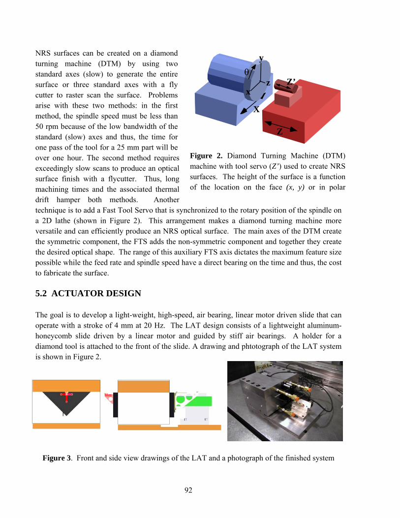
92

NRS surfaces can be created on a diamond turning machine (DTM) by using two standard axes (slow) to generate the entire surface or three standard axes with a fly cutter to raster scan the surface. Problems arise with these two methods: in the first method, the spindle speed must be less than 50 rpm because of the low bandwidth of the standard (slow) axes and thus, the time for one pass of the tool for a 25 mm part will be over one hour. The second method requires exceedingly slow scans to produce an optical surface finish with a flycutter. Thus, long machining times and the associated thermal drift hamper both methods. Another technique is to add a Fast Tool Servo that is synchronized to the rotary position of the spindle on a 2D lathe (shown in Figure 2). This arrangement makes a diamond turning machine more versatile and can efficiently produce an NRS optical surface. The main axes of the DTM create the symmetric component, the FTS adds the non-symmetric component and together they create the desired optical shape. The range of this auxiliary FTS axis dictates the maximum feature size possible while the feed rate and spindle speed have a direct bearing on the time and thus, the cost to fabricate the surface. 5.2 ACTUATOR DESIGN The goal is to develop a light-weight, high-speed, air bearing, linear motor driven slide that can operate with a stroke of 4 mm at 20 Hz. The LAT design consists of a lightweight aluminum-honeycomb slide driven by a linear motor and guided by stiff air bearings. A holder for a diamond tool is attached to the front of the slide. A drawing and phtotograph of the LAT system is shown in Figure 2.

Figure 3. Front and side view drawings of the LAT and a photograph of the finished system

x

y

z

Z

Z’

X

θ

Figure 2. Diamond Turning Machine (DTM)machine with tool servo (Z’) used to create NRSsurfaces. The height of the surface is a functionof the location on the face (x, y) or in polar

93

5.2.1 SLIDE MATERIAL The first step in the axis design was to select a material for the slide and develop the shape of the cross-section. The slide required a small moving mass, high stiffness to produce a high natural frequency for the system and sufficient surface area to produce a stiff air bearing. For these reasons, aluminum honeycomb was selected as the working material. Aluminum honeycomb consists of a honeycomb core of thin aluminum sheet sandwiched between two thicker aluminum faces. The core cell structure holds the face sheets apart to generate the high bending stiffness but its low shear strength tends to decrease the theoretical stiffness by about 80%. The properties of flat honeycomb samples were calculated and measured, and a model for the actual material properties based on modulus and density was constructed. This model was used in the analysis discussed next. 5.2.2 FEM ANALYSIS To select an optimum cross-section shape, finite element models were created for different candidate shapes. Three basic shapes were analyzed: a box, a V-shape, and a triangle, as illustrated in Figure 4. The properties of interest are the bending stiffness, mass, first natural frequency, center of gravity, location of the linear motor and location of the position sensing encoder.

Figure 4: From left to right, the box, V-shape, and triangular slide designs After simulating static bending as well as dynamic mode shapes for each slide design, the box geometry was eliminated because removal of material to embed the motor caused a large drop in natural frequency. The remaining designs were compared using data obtained from simulations as shown in Table 1.

Table 1: Comparison of V Shape and Triangle slide designs

Mass (g) Nat.Freq. (Hz) Lateral stiffness (N/µm) Vertical stiffness (N/µm) # Parts V Shape 400 3450 8.145 8.17 4 Triangle 445 3950 25 10.5 2

94

Although slightly heavier, the triangular cross-section was selected because it proved more resistant to static forces such as tool-tip loads, displayed a higher natural frequency than the V shape and required a housing structure with the least number of parts, simplifying the assembly. 5.2.3 SLIDE LENGTH Another important design issue is the length of the moving slide. As the slide length increases, the bearing stiffness and natural frequency increase due to the larger surface area. However, the structural natural frequency of the moving slide decreases as the length increases. After analyzing the changes in natural frequency and the rate of change of stiffness with bearing length, a 7” slide was selected as the optimum length. 5.2.4 MOTOR SELECTION A brushless linear motor was chosen for its smooth motion characteristics, high accuracy, repeatability, high acceleration capabilities and stiffness. To reduce the moving mass of the system, the smallest/lightest motor capable of producing enough continuous force to drive the system was desired. Equation (1) was used to determine the force needed to drive the system:

F = mAω2 (1)

where m is the mass in Kg, A is the amplitude in m and ω is the frequency in rad/sec. For an assumed moving mass of 500 g, an operating frequency of 20 Hz, and an amplitude of 2 mm (for a total stroke of 4 mm), 15.8 N are needed to drive the system. From the Airex Linear Motor P12 Series, the P12-1 is chosen (continuous force 27 N [2]). This motor weighs 100 g. 5.2.5 MOUNTING BRACKET The motor mount bracket connects the motor to the slide. The bracket must support the full weight of the motor, provide a rigid coupling to the slide and have minimum weight. The first bracket tested had a square faceplate to be bolted to the rear of the slide and a channel with 1.5 mm thick walls and vertical gussets to contain the motor. However, this bracket was disappointingly flexible, allowing too much deflection between the motor and slide. As a result of modeling, the faceplate was made taller to provide more resistance against vertical bending; also horizontal gussets were added. Lightweighting holes were also added to the bracket in non-critical locations to reduce the mass.

Figure 5: Improvedfinal bracket

95

The new bracket, shown in Figure 5, performed well in dynamic simulations. The natural frequency of the slide-bracket-motor system was increased by nearly 50% and deformation was similar to that predicted for the slide and motor, indicating sufficient bracket stiffness. 5.2.6 EXPERIMENTAL VERIFICATION When the moving slide was fabricated, accelerometers were used to observe its dynamic characteristics and compare those results to the predicted behavior. A free-free natural frequency test was used both with and without the motor and bracket. The setup for the experiment is shown in Figure 6.

Figure 6. Setup for frequency analysis

A hammer was used to strike the slide resting on soft foam. The attached accelerometer then reported the vibration. The results are given below in Table 2.

Table 2: Experimental results for natural frequency test (moving slide only)

With the values for the first and second natural frequencies showing a near match, two accelerometers were used to observe the vibration at different spots simultaneously on the slide. The relative magnitude and phase data of the two positions confirmed the predicted mode shapes – a twisting motion at the first frequency and a bending mode at the second. 5.2.7 LINEAR ENCODER The Renishaw RGH24B linear encoder provides position feedback to the UMAC controller for position control and to the amplifier for commutation. The encoder scale is in the form of a steel tape and is attached to the top of the slide via an adhesive backing. The readhead is rigidly attached to the structure of the bearing. The encoder signal period is 20 µm. The 1 V p-p

1st Natural Frequency (Hz) 2nd Natural Frequency (Hz) Ratio of First/Second Predicted Results 3950 5110 0.77 Actual Results 3540 4660 0.76

96

sinusoidal output is interpolated by the UMAC into 4096 counts per period, giving it a theoretical resolution of 5 nm. During initial machining tests, PWM noise from the X- and Z-axis amplifiers limited the actual resolution to approximately 100 nm. Subsequent line filtering improved this figure to slightly better than 50 nm. 5.2.8 TOOL HOLDER Precitech designed a light-weight tool holder pictured in Figure 7, which attaches to the front of the triangular piston. The diamond tool is mounted on a standard commercial indexing-style insert that is bolted to the tool holder. The tool is in line with the linear encoder that is attached to the piston, so there is no Abbe offset in the position measurement.

Figure 7. Tool holder and diamond tool mounted on the front of the triangular piston

5.3 ACTUATOR FABRICATION The piston, air-bearings and housing were fabricated at Precitech and at local contractors in the Keene, NH area. Two pistons were fabricated. The first was used for dynamic testing and the second was assembled into the air bearing and used for machining experiments. 5.3.1 AIR BEARING DESIGN A base assembly and a top, as shown in the overall photograph of Figure 3, support the triangular piston. The base assembly is composed of a v-block with two thin etched plates brazed on the face of the bearing surfaces. These plates incorporate an innovative air bearing design and fabrication procedure. The air bearing assembly includes eight replaceable brass orifices; and external pneumatic fittings (see Figure 3) were provided to permit development of the dynamic stiffness. The bearings in the base assembly were optimized for stiffness and damping in frequency range of the first dominant vibration mode. The brazed assembly is precision ground

97

to provide precise air film gaps with the cap and slide assembly, which can be fine tuned at assembly. The upper air bearing in the top plate was designed primarily to provide preload for the two lower air bearings. This greatly relieves the manufacturing tolerances. All surfaces were lapped to improved flatness and finish and the final straightness on average was less than 0.0001” (2.5 µm) and the finish was 20 µin or 0.5 µm. Alignment of the finished 90 degree v-block to the bottom of the base was accomplished by inserting the Slide/Piston into the v-block, turning the piston and base over, and placing the top of the piston on a block of steel that would be ground in place on a surface grinder. Then the bottom of the base was clean ground. After the bottom was ground, the top of the base was re-ground relative to the bottom. The piston was then inserted into the base, and the initial clearance of 0.0018” (45 µm) was ground into the base. 5.3.2 PISTON AIR BEARING STIFFNESS Stiffness measurement was done with the base sitting on a granite plate and with a bridge built from steel, which was used to support a 10 lb test weight as shown in Figure 8. The piston was protruding approximately 0.60” from each end of the base/top plate. Precision ground risers were placed on each end of the piston as a base to form the test bridge assembly and 80 psi of air was applied to the entire assembly.

Figure 8. Measurement of the piston air bearing stiffness The 10 lb test weight was placed in the center of the bridge, and the electronic indicator was positioned on the end of the piston. The indicator showed 5-7 µin of deflection, indicating a stiffness of 1.67 million lb/in. Then, the test weight was moved from the central position on the test bridge to the end of the test bridge, directly over the indicator. Now the indicator showed 30-

98

35 µin of deflection. Stiffness was 300,000 lb/in. For this test, the magnetic base supporting the electronic indicator was positioned on the top plate in order to minimize deflection in the measurement loop. The air flow to the piston was measured. Flow measurements on the base with 80 psi applied were 94 liter/min. Flow measurements on the top plate with 80 psi applied were 96 liter/min. 5.4 DYNAMIC TESTING One major concern in attaching the LAT system to the Z-axis of the Nanoform 600 DTM was the effect it would have on the motion of the Z-axis. Initial estimates showed that, given the baseline design parameters, the impact on the Z-axis would not be significant due to the high stiffness of the Z-axis and the small moving mass of the LAT axis compared to the Z-axis. For a LAT amplitude of 2 mm amplitude at 20 Hz, the force generated on the Z-axis by the 0.657 Kg moving mass will be 21 N (F=mAω2).

• Nanoform 600 (Testbed) Z-slide stiffness: k=6X107 N/m • Static Deflection: @ 21 N = 0.345 µm • Dynamic Z-Slide Deflection @ 20 Hz (ignoring viscous damping and nonlinear coupling):

DTM Z slide mass = 105 Kg For 21 N amplitude, A=F/(k-mω2) = (21 N)/( 6X107 N/m - 105 kg*(20*2π)2)=0.36 µm

The small difference between the static deflection and the dynamic deflection is a result of the large difference between the excitation frequency (20 Hz) and the natural frequency of the Z-slide (105 Hz).

Figure 9. Motion of the Z-axis of the DTM with the LAT performing a 2 mm, 20 Hz sine wave

99

If this deflection only occurred at the excitation frequency (as it would with a linear system), the result would be an apparent reduction in the amplitude of the servo motion and that reduction could be compensated with increased gain. However, the low frequency servo motion excites the Z-slide at its natural frequency (105 Hz) as shown in Figure 9. The relative motion of the Z-slide at the 105 Hz natural frequency is larger than that at the excitation frequency of 20 Hz. This high frequency motion will have a deleterious effect on the surface finish and some remedy must be developed to reduce this effect. Several ideas including counter-balance masses and tuned dampers will be examined in a later phase of the project. 5.5 CONTROL SYSTEM DEVELOPMENT The LAT system was integrated into the Nanoform 600 diamond turning machine for the machining experiments. The machine controller, a Delta Tau Turbo UMAC, allowed this new axis to be added to the system without compromising performance or flexibility. The existing user interface was used to input the commands to the LAT slide and evaluate the motion of the tool with respect to the commanded position.

����

�������

��� � �

� ���������� ������� �

�� ��

���� ����� �

���������������

�������� ���

������ �

Figure 10. Diagram of general control system layout As shown in Figure 10, the UMAC controller on the DTM controlled the LAT axis as well as the other linear axes (X and Z) and the spindle. This setup, as opposed to one where a separate system controls the LAT axis, was chosen to simplify the integration problems. The controller for the LAT axis must know the positions of the other axes, including the spindle, in order to

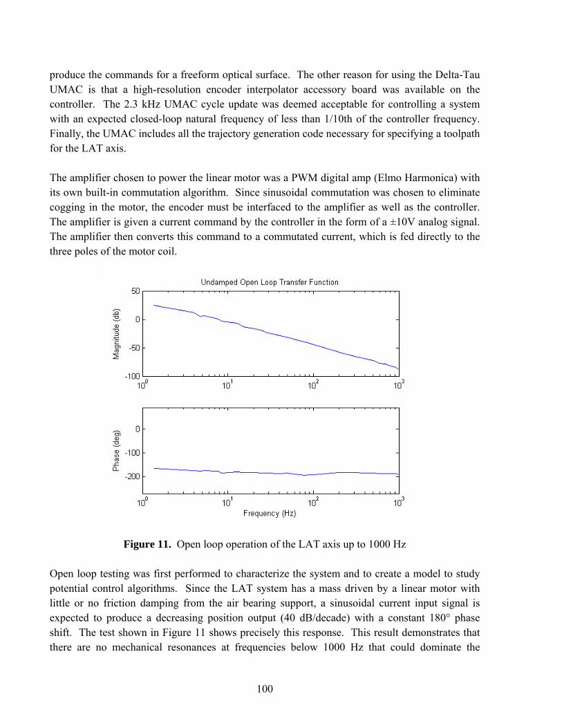
100

produce the commands for a freeform optical surface. The other reason for using the Delta-Tau UMAC is that a high-resolution encoder interpolator accessory board was available on the controller. The 2.3 kHz UMAC cycle update was deemed acceptable for controlling a system with an expected closed-loop natural frequency of less than 1/10th of the controller frequency. Finally, the UMAC includes all the trajectory generation code necessary for specifying a toolpath for the LAT axis. The amplifier chosen to power the linear motor was a PWM digital amp (Elmo Harmonica) with its own built-in commutation algorithm. Since sinusoidal commutation was chosen to eliminate cogging in the motor, the encoder must be interfaced to the amplifier as well as the controller. The amplifier is given a current command by the controller in the form of a ±10V analog signal. The amplifier then converts this command to a commutated current, which is fed directly to the three poles of the motor coil.

Figure 11. Open loop operation of the LAT axis up to 1000 Hz

Open loop testing was first performed to characterize the system and to create a model to study potential control algorithms. Since the LAT system has a mass driven by a linear motor with little or no friction damping from the air bearing support, a sinusoidal current input signal is expected to produce a decreasing position output (40 dB/decade) with a constant 180° phase shift. The test shown in Figure 11 shows precisely this response. This result demonstrates that there are no mechanical resonances at frequencies below 1000 Hz that could dominate the

101

motion of the axis. The mechanical system can thus be considered to behave as it was designed. Based on the measurements of the triangular piston alone, the first resonance should be above 2.5 KHz but the dynamics of the air bearing could introduce other dynamics.

����

���������� � � ����

������� �� � ���!�"��#

�� � ��

�������

Figure 12. Control loop for the LAT axis The next step was to close the loop using position feedback to control the postion of the tool. The system looks like the diagram in Figure 12. The amplifier operates in current mode and provides a force to the LAT through the linear motor. The motion of the slide is measured with the encoder and this is compared with the commanded position at each time step to produce a difference signal that is the input to the control algorithm in the machine controller. The digital algorithm is used to change the gain and phase of the LAT axis, such that the output follows the commanded signal up to some frequency dependent on the algorithm and gains selected.

Figure 13. Closed loop Bode plots for the LAT system

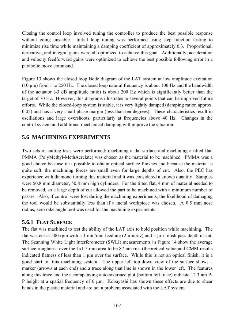
102

Closing the control loop involved tuning the controller to produce the best possible response without going unstable. Initial loop tuning was performed using step function testing to minimize rise time while maintaining a damping coefficient of approximately 0.3. Proportional, derivative, and integral gains were all optimized to achieve this goal. Additionally, acceleration and velocity feedforward gains were optimized to achieve the best possible following error in a parabolic move command. Figure 13 shows the closed loop Bode diagram of the LAT system at low amplitude excitation (10 µm) from 1 to 250 Hz. The closed loop natural frequency is about 100 Hz and the bandwidth of the actuator (-3 dB amplitude ratio) is about 200 Hz which is significantly better than the target of 70 Hz. However, this diagrams illustrates to several points that can be improved future efforts. While the closed-loop system is stable, it is very lightly damped (damping ration approx. 0.05) and has a very small phase margin (less than ten degrees). These characteristics result in oscillations and large overshoots, particularly at frequencies above 40 Hz. Changes in the control system and additional mechanical damping will improve the situation. 5.6 MACHINING EXPERIMENTS Two sets of cutting tests were performed: machining a flat surface and machining a tilted flat. PMMA (PolyMethyl-MethAcrelate) was chosen as the material to be machined. PMMA was a good choice because it is possible to obtain optical surface finishes and because the material is quite soft, the machining forces are small even for large depths of cut. Also, the PEC has experience with diamond turning this material and it was considered a known quantity. Samples were 50.8 mm diameter, 50.8 mm high cylinders. For the tilted flat, 4 mm of material needed to be removed, so a large depth of cut allowed the part to be machined with a minimum number of passes. Also, if control were lost during the machining experiments, the likelihood of damaging the tool would be substantially less than if a metal workpiece was chosen. A 0.5 mm nose radius, zero rake angle tool was used for the machining experiments. 5.6.1 FLAT SURFACE The flat was machined to test the ability of the LAT axis to hold position while machining. The flat was cut at 500 rpm with a 1 mm/min feedrate (2 µm/rev) and 5 µm finish pass depth of cut. The Scanning White Light Interferometer (SWLI) measurements in Figure 14 show the average surface roughness over the 1x1.5 mm area to be 87 nm rms (theoretical value and CMM results indicated flatness of less than 1 µm over the surface. While this is not an optical finish, it is a good start for this machining system. The upper left top-down view of the surface shows a marker (arrows at each end) and a trace along that line is shown in the lower left. The features along this trace and the accompanying autocovariace plot (bottom left trace) indicate 12.3 nm P-P height at a spatial frequency of 6 µm. Kobayashi has shown these effects are due to shear bands in the plastic material and are not a problem associated with the LAT system.

103

Figure 14. Scanning White Light Interferometer (SWLI) image of the machined flat The shear bands account for less than 5% of the surface roughness for the flat surface. The cause of the remainder of the surface error cannot be directly deduced from the surface measurement, though indirect evidence shows two likely sources: Encoder signal noise and a resonance in the axis control. Noise associated with the PWM (pulse width modulation) amplifiers used to power the linear and spindle axes of the DTM is present in the analog encoder signal. This noise occurs primarily at the 28 KHz modulation frequency, but through various ground paths becomes a broad-band quasi-white noise. With this noise on the encoder signals, the position feedback signal read by the control algorithm contained a significant error. As a result, the controller failed to accurately position the axis. This is a vulnerability of the chosen encoder feedback system where an analog sinusoidal signal is read directly by the controller as opposed to going through an interpolator box that then sends a digital position feedback signal. Reading the sine wave signals directly was selected because of the need to measure the position at both high resolution and high velocity. Once the noise problem was identified, it was improved by adding line filters to the axis motors. The resonance in the axis control system was another source for the high surface roughness measured on the flat surfaces. The axis error during machining is shown in Figure 15 along with the frequency content. The time plot over one second shows peaks with a magnitude of 1.6 µm

104

which is similar to the surface roughness of the machine flat. The major frequency identified is 265 Hz. The origin of this peak is not known but a similar value was present during machining of the tilted flat. Future efforts will involve identification of the source of this vibration and reducing its effect using controller design, mechanical damping and counter balancing designs.

Figure 15. Error motion (left) of the LAT axis (commanded minus actual position) during machining at 500 rpm. The figure at right is the FFT of the error. 5.6.2 TILTED FLAT A second experiment involved the fabrication of a tilted flat. A sketch of this experiment is shown in Figure 16 with the LAT slide moving the tool in a sine wave motion with one cycle per rotation of the part. The LAT slide is programmed to generate a particular depth at each rotary encoder location. As the tool moves from the OD to ID, the tool will move in and out once per revolution to create a flat surface that is tilted with respect to the spindle face

Tool motion = A sin f θ

Rotating spindle

LAT

Figure 16. Top view of DTM during generation of tilted flat.

105

The tilted flat was machined using 500 rpm, 2.5 mm/min feedrate (5 µm/rev) and 5 µm final pass depth of cut. Roughing cuts were first performed using a 100 µm depth to rough cut the slope on the part. The final surface had an average roughness of 412 nm and a figure error of 47 µm.

Figure 17. Surface roughness on the 4 mm tilted flat. The radial direction is approximately along the grooves.

A sample roughness measurement over a 719x539 µm region is shown in Figure 17. This region is about 5 times larger than the flat in Figure 14 and represents 144 passes of the tool. Two features dominate the shape of the tilted flat; one is an undulation in the radial direction with a spatial wavelength of 400 µm and the other is lower amplitude but parallel feature with a wavelength of 60 µm. These features are likely due to vibration of the LAT axis. While the amplitudes of vibration of the axis and those measured on the surface are of similar magnitude, correlating any one of the multitude of vibrations of the axis to the many surface defects is not possible. Figure 18 shows the time signal and frequency spectrum of the position error (commanded position minus the encoder reading) recorded during the machining of the tilted flat. The FFT shows many resonances mainly occurring at around 65 and 250 Hz surrounded by several harmonics.

106

Figure 18. Error motion (left) of the LAT axis (commanded minus actual position) during machining at 500 rpm with 8.3 Hz error removed. FFT of the error is shown at right.

5.6.3 FIGURE ERROR Figure error for both the flat surface and the tilted flat was to be measured using a Zygo GPI laser interferometer. Due to the greater than expected roughness and the low reflectance of PMMA, however, measurements could not reliably be made through interferometry. Instead, figure measurements were made using a Brown & Sharpe Gage 2000 Coordinate Measuring Machine (CMM) shown in Figure 19. While this instrument has a substantially lower resolution (1 µm) than the laser interferometer (0.1 nm), errors in the tilted flat are currently still large enough not to require such high resolution. The non-tilted flat, on the other hand, was found to be flat to better than 1 µm – beyond the capability of the CMM. The tilted flat has a P-V error of 46 µm. Further improvements in control schemes and noise reduction in the system will reduce this figure error significantly.

Figure 19. Tilted flat being measured by the CMM

Frequency (Hz) Time (s) Time (s)

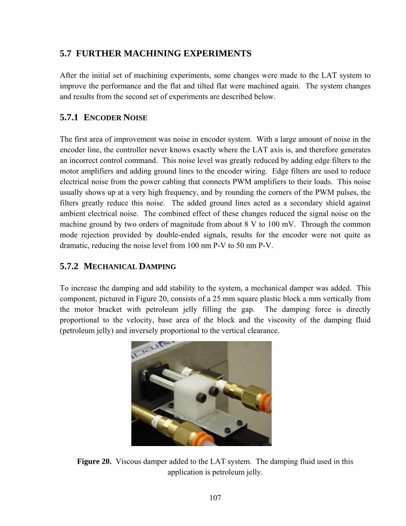
107

5.7 FURTHER MACHINING EXPERIMENTS After the initial set of machining experiments, some changes were made to the LAT system to improve the performance and the flat and tilted flat were machined again. The system changes and results from the second set of experiments are described below. 5.7.1 ENCODER NOISE The first area of improvement was noise in encoder system. With a large amount of noise in the encoder line, the controller never knows exactly where the LAT axis is, and therefore generates an incorrect control command. This noise level was greatly reduced by adding edge filters to the motor amplifiers and adding ground lines to the encoder wiring. Edge filters are used to reduce electrical noise from the power cabling that connects PWM amplifiers to their loads. This noise usually shows up at a very high frequency, and by rounding the corners of the PWM pulses, the filters greatly reduce this noise. The added ground lines acted as a secondary shield against ambient electrical noise. The combined effect of these changes reduced the signal noise on the machine ground by two orders of magnitude from about 8 V to 100 mV. Through the common mode rejection provided by double-ended signals, results for the encoder were not quite as dramatic, reducing the noise level from 100 nm P-V to 50 nm P-V. 5.7.2 MECHANICAL DAMPING To increase the damping and add stability to the system, a mechanical damper was added. This component, pictured in Figure 20, consists of a 25 mm square plastic block a mm vertically from the motor bracket with petroleum jelly filling the gap. The damping force is directly proportional to the velocity, base area of the block and the viscosity of the damping fluid (petroleum jelly) and inversely proportional to the vertical clearance.

Figure 20. Viscous damper added to the LAT system. The damping fluid used in this

application is petroleum jelly.

108

5.7.3 NOTCH FILTER Finally, a notch filter was added to the controller to eliminate the sharp peak around 250 Hz seen during the first flat surface machining experiment (Figure 18). The effect of the notch filter is shown in Figure 21. The top graph shows the old system FFT (excluding 8.3 Hz) without the notch filter. The bottom shows the system with the addition of the notch filter, which effectively removes the 250 Hz frequency.

Figure 21. The effect of the notch filter in the controller on the system performance

5.7.4 FLAT SURFACE Surface finish After the changes were made to the system, another flat was machined. The cutting parameters were the same as those for the original flat. The Scanning White Light Interferometer (SWLI) measurements in Figure 22 show the average surface roughness over the 0.7X0.5 mm area to be 87 nm rms.

109

Figure 22. Scanning White Light Interferometer (SWLI) image of the second machined flat Figure Measurement Since the surface finish of the second flat was much better than the first, it could be measured using the Zygo GPI laser interferometer. Figure 23 shows a total figure error of 800 nm over the entire part, with an RMS of 87 nm. These numbers show a much better surface than originally machined, indicating improved performance from the LAT axis. 5.7.5 TILTED FLAT

The second tilted flat was machined at 500 rpm, 2.5 mm/min feedrate (5 µm/rev) and 5 µm final depth of cut (same parameters as original cut). However, this tilted flat only had a P-V height of 2 mm. The results from this experiment were similar to those in the first experiment. The surface was again dominated by undulations occurring at two spatial frequencies: roughly 400 µm and 60 µm. For the new tilted flat (again using the Brown & Sharpe CMM), the figure error was 54 mm. Upon further examination of the data, it was noted that this figure error was dominated by an error in tool centering in the x-direction. While tool centering is not important when machining a flat, in the case of a tilted flat, the primary excursion of the LAT axis is

110

sinusoidal as a function of X-axis position. If the X-axis position is incorrect, a characteristic error results.

Figure 23. Figure error of the second machined flat measured by the Zygo laser interferometer.

5.8 CONCLUSIONS AND FUTURE WORK Preliminary results from experiments conducted at the PEC show the Live-Axis Turning system to be a viable means of fabricating non-rotationally symmetric surfaces (NRS). A flat surface and a tilted flat have been produced, showing the error when holding position and performing a high-speed, high-amplitude trajectory. While these surfaces are not yet optical quality, the results are a good start for this machining system. A proposal for a Phase II effort has been submitted and, if funded, additional work will conducted including:

• General mechanical improvements – This category will include an encoder that creates less noise and a new linear motor amplifier. Also, a counter-balance or tuned damper will be considered to minimize the reaction forces from the LAT system that affect the z-axis motion.

111

• Mechanical Damping – The addition of damping on the slide is important to creating a stiff, stable control system.

• Controller optimization – Control design has been completed on the system, but a more in-depth scheme with other types of controllers will be studied to improve system performance.

• New motion program for machining – While the programs for the flat and tilted flat were basic motion programs implemented on a Delta Tau UMAC controller, use of the controller’s inverse kinematics programming may improve signal following error.

112

REFERENCES 1. Garrard, K.P., A. Sohn, R. G. Ohl, R. Mink, V. J. Chambers. “Off-Axis Biconic Mirror

Fabrication.” Proceedings from the EUSPEN 2002 Annual Meeting (2002). 2. Airex Corporation. Dover, New Hampshire, http://www.airex.com 3. Lin, C. L. “Multiobjective PID Control for a Brushless Linear Motor: An Evolutionary

Approach.” IEE Proceedings Electric Power Applications, v 149, No. 6, Nov 2002, p. 397-406.

113

6 METROLOGY ARTIFACT DESIGN

Karalyn Folkert Graduate Student

Kenneth Garrard Precision Engineering Center Staff

Thomas A. Dow Professor

Department of Mechanical and Aerospace Engineering After a part has been manufactured, the part is measured to determine whether it is within its tolerance region. These measurements are often taken on Coordinate Measuring Machines (CMMs). The dynamics of the CMM influence the overall measurement. Traditionally, a calibration artifact determines the static influences of the machine, such as machine geometry. The goal of this project is to design and fabricate a calibration artifact that will test the CMM dynamically and determine the effects of those influences. The artifact developed is a ring gauge to represent the typical size of parts manufactured by the Y-12 National Security Complex (Y-12). On the ring gauge, small swept sine wave features are placed on the inside and outside diameter. A swept sine wave is a sine wave that continuously varies its frequency. The range of frequencies creates a window for evaluation of the machine capabilities. The transfer function of the CMM dynamics is found by comparing the accepted swept sine wave with the measured wave. By knowing the magnitude and phase characteristics of the dynamic system, the operator can make decisions referring to the machine’s capabilities based on the measurement speed. Issues relating to fabrication, measurement, and data analysis will be discussed.

114

6.1 INTRODUCTION The Y-12 National Security Complex (Y-12) manufactures precision work pieces for the government and private companies. Part acceptance is based on dimensional inspection by comparison to the tolerance specifications of the part drawing. The goal of this project is to design and fabricate an artifact that can accurately predict the measurement uncertainty for a specific task, such as scanning around a workpiece by determining a transfer function associated with the machine. 6.2 CMM A CMM consists of three carriages that are mutually orthogonal. Each machine may have a different configuration. In Figure 1, the three axes are able to move while the table remains fixed. Displacement transducers are fixed along each linear axis of the CMM, which allows a spatial reference point on the probe to be used to determine the displacement along a coordinate path in the working volume of the CMM.

Figure 1. Moving bridge CMM at NCSU. In Figure 1, the probe is attached to the end of the z-axis carriage. As the carriages move and the probe contacts the surface of a work piece, the probe takes a coordinate measurement reading at the point of contact. The probe is an integral part of the CMM but increases the inherent error of the CMM. 6.2.1 CALIBRATION OF CMMS There is an important need to quantify the capability of measuring machines to characterize the dimensional features of 3-D work pieces. For a given measurement task, different machines and

115

measurement procedures will produce different results depending on the shape, weight and surface features of the part. Over the years, significant effort has been expended to find methods to reduce errors in a measuring machine [1]. Typically, the working volume is divided into regions and the position errors in each region are defined in the x, y and z directions. This error information can be put into look-up tables on the machine controller and the actual part dimensions can be determined based on compensating the machine measurements for the errors in position from the error map. The uncertainty in the measurement result will involve the size of the error and the repeatability of that error for a specific machine position. Error mapping the entire working volume of the CMM provides one solution for calibration by correcting the slide position based on the position of the probe [1]. Error mapping of the CMM highlights the parametric errors of the machine but does not consider the dynamic errors during a measurement. The complexity of a part will greatly increase the resulting measurement error due to the increased complexity of the CMM motion [2]. Accordingly, higher measurement speeds will result in higher accelerations when measuring anything other than a flat surface. The changing accelerations will magnify the static geometric errors; since these errors are dependant on carriage positions, the acceleration of one carriage will vary the moment applied to another carriage [2]. One way to estimate dynamic errors is to use additional sensors attached to each carriage of the CMM and to construct a kinematic model to estimate probe position [2]. However, this method only demonstrates improved measurement accuracy with single axis motion. Instead of modeling the dynamic errors of the machine, an artifact may be designed to determine the actual dynamic characteristics of the machine. To address more measurement specific errors, the artifact should be the approximate size and weight of a typical work piece. Therefore, if boxes are to be measured, then a box of roughly the same size, shape and weight of the box to be measured should be calibrated. The artifact box or series of artifact boxes must exhibit the typical errors of the boxes to be measured to validate the machine capability relative to those types of errors. However, to test the dynamic limits of the CMM, features need to be designed into the artifact. These features may simulate various conditions that the probe may encounter on a part. Some other major considerations for an artifact are ease of use, transportability, stability, time needed for calibration and ability to diagnose the error [1]. 6.3 RING GAUGE There have been a number of calibration artifacts developed including ball bars, ball and hole plates, ring gauges, and hole bars [3]. After considering these artifact standards, a ring gauge was chosen for further development. The overall attributes of the ring gauge (outside diameter (OD), inside diameter (ID), width and wall thickness) can be used to exercise multiple axes of a

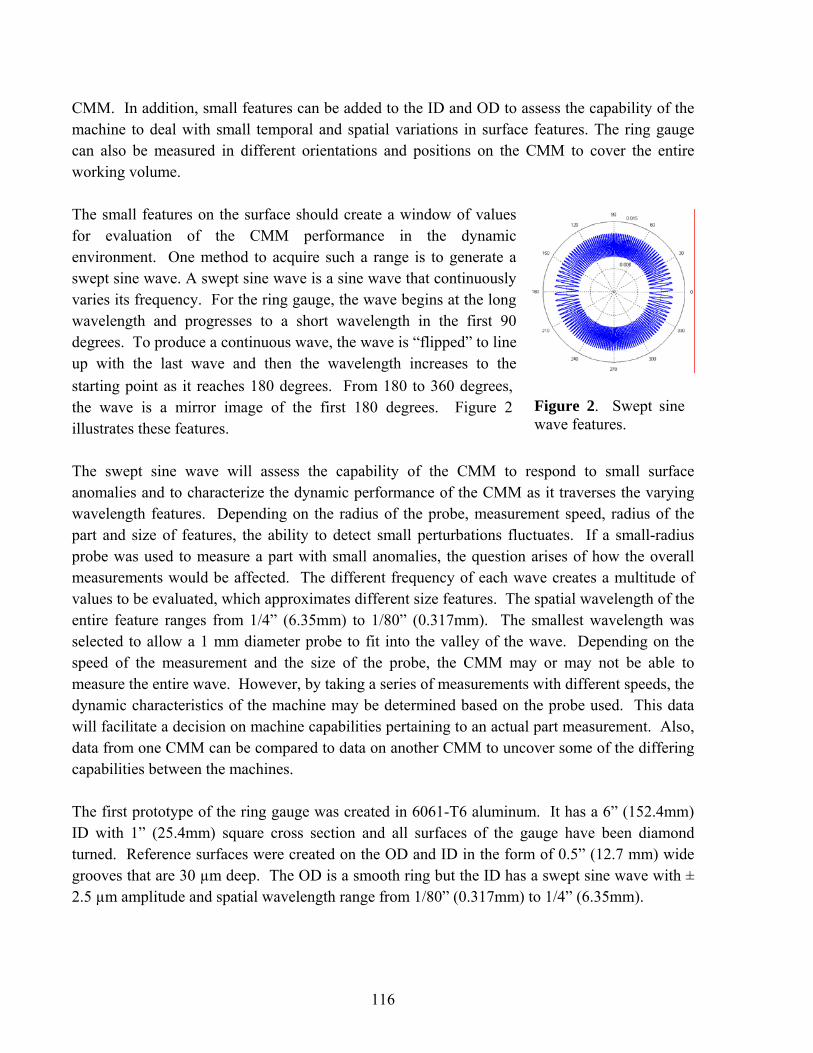
116

CMM. In addition, small features can be added to the ID and OD to assess the capability of the machine to deal with small temporal and spatial variations in surface features. The ring gauge can also be measured in different orientations and positions on the CMM to cover the entire working volume. The small features on the surface should create a window of values for evaluation of the CMM performance in the dynamic environment. One method to acquire such a range is to generate a swept sine wave. A swept sine wave is a sine wave that continuously varies its frequency. For the ring gauge, the wave begins at the long wavelength and progresses to a short wavelength in the first 90 degrees. To produce a continuous wave, the wave is “flipped” to line up with the last wave and then the wavelength increases to the starting point as it reaches 180 degrees. From 180 to 360 degrees, the wave is a mirror image of the first 180 degrees. Figure 2 illustrates these features. The swept sine wave will assess the capability of the CMM to respond to small surface anomalies and to characterize the dynamic performance of the CMM as it traverses the varying wavelength features. Depending on the radius of the probe, measurement speed, radius of the part and size of features, the ability to detect small perturbations fluctuates. If a small-radius probe was used to measure a part with small anomalies, the question arises of how the overall measurements would be affected. The different frequency of each wave creates a multitude of values to be evaluated, which approximates different size features. The spatial wavelength of the entire feature ranges from 1/4” (6.35mm) to 1/80” (0.317mm). The smallest wavelength was selected to allow a 1 mm diameter probe to fit into the valley of the wave. Depending on the speed of the measurement and the size of the probe, the CMM may or may not be able to measure the entire wave. However, by taking a series of measurements with different speeds, the dynamic characteristics of the machine may be determined based on the probe used. This data will facilitate a decision on machine capabilities pertaining to an actual part measurement. Also, data from one CMM can be compared to data on another CMM to uncover some of the differing capabilities between the machines. The first prototype of the ring gauge was created in 6061-T6 aluminum. It has a 6” (152.4mm) ID with 1” (25.4mm) square cross section and all surfaces of the gauge have been diamond turned. Reference surfaces were created on the OD and ID in the form of 0.5” (12.7 mm) wide grooves that are 30 µm deep. The OD is a smooth ring but the ID has a swept sine wave with ± 2.5 µm amplitude and spatial wavelength range from 1/80” (0.317mm) to 1/4” (6.35mm).

Figure 2. Swept sinewave features.

117

The material chosen for the trial fabrication of the ring gauge was Aluminum 6061-T6. Al 6061 was selected for its ease of machineability and its prevalence. One of the attributes of Al 6061 is its high coefficient of thermal expansion. The size of the part may change a significant amount depending on the temperature of its environment. For calibration purposes, it is important that the artifact not fluctuate in size. Thus, the material for the final artifact is 17-4 PH stainless steel which will be heat treated for thermal stability. Stainless steel cannot be machined with a diamond tool due to the amount of damage possible to the tool. For this reason, the ring is plated with Electroless Nickel, which exhibits a non-ferrous characteristic, making diamond tool machining permissible. The plating also adds to the microhardness; the actual quantity is dependant on the phosphorus content of the plating. 6.3.1 FABRICATION OF SWEPT SINE WAVE The wave features of the artifact are fabricated using a Fast Tool Servo (FTS) shown in Figure 3. An 18 mm long, hollow cylindrical piezoelectric actuator (25 mm OD and 12 mm ID) drives the device to a maximum displacement of 18 µm. A capacitance gage provides feedback on the position of the tool holder by observing the movement of the base plate through the hollow actuator. A commanded position is turned into a positive input voltage and sent to a high voltage amplifier where it is amplified by 100 before being sent to the FTS.

Figure 3. Fast Tool Servo. Figure 4. System dynamics of the FTS. The open-loop dynamics of the FTS as a function of the frequency of a sine wave command is shown in Figure 4. The top graph is the amplitude ratio of the output voltage from the capacitance gage to the input voltage to the amplifier. It shows a slight decrease in amplitude with frequency up to about 400 Hz and a strong increase to the first natural frequency of about 5 kHz. This frequency is a result of the first bending mode of the cylindrical plate that serves as the base for the tool holder. The phase difference between input and output shows a small offset (3˚) at DC that grows to about 27˚ at 1000 Hz

118

6.3.2 CONTROL OF THE FTS The FTS has high order characteristics (Figure 4) that will greatly impede the accuracy of the features. For this reason, closed loop control will be used to control the FTS. The swept sine wave will be cut into the surface in the 10 to 600 Hz range. Even in this range, there is a change in the magnitude as well as phase. There is an initial phase lag of 3° that increases to 7°. One complication when using piezoelectric actuators (PZTs) is that they add hysteresis to the motion and, as a result, the gain for the system is a function of the amplitude. Figure 5 illustrates this phenomenon. The three curves are for 100%, 75% and 20% of the range of motion. Note that the peak-to-peak (P-P) voltage divided by the P-P motion is not a constant: it varies from 1.846 to 1.365 at 100% and 20% respectively. This is a significant drop in gain; 25% from the full range to 20% of full range. As a result, the open-loop transfer function will change with different amplitudes of the swept sine wave. Such non-linear behavior may complicate control for an arbitrary input shape.

Figure 5. Hysteresis loops for different amplitudes of motion for the PZTs in the FTS. Feedback control can correct for position error at low frequency. The closed loop control uses feedback from the capacitance gage position sensor along with proportional-integral (PI) control algorithm to correct position error. The gains were chosen based on the best possible response of the system. The purpose of this closed loop control is to shape the response of the system, prevent overshoot and correct for the following error. A proportional gain of 0.3 is used to produce a constant magnitude with the chosen integral gain. The integral gain controls how quickly the system reaches its intended input. A gain of 10,000 has been chosen.

119

Figure 6. Comparison of closed loop and open loop system identifications up to 600 Hz. Figure 6 shows the closed loop system response as compared to the open loop response and also demonstrates the change in the transfer function as the amplitude changes. The dot and circle markers correspond to the closed loop system with amplitude inputs of 1 µm and 5 µm, respectively. The triangle marker represents the open loop response of the system. The magnitude remains constant in the operating range of interest for the closed loop responses. There is less phase lag at low frequency with the 1µm input but it becomes larger than the open loop value for frequencies greater than 100 Hz. However, for the desired amplitude of 5µm, the phase and magnitude are always better than the open loop system. If the swept sine wave were machined using this closed loop control system, the phase in the higher frequency waves would still put them out of position by 15˚. To reduce the effect of the FTS phase lag, the phase will be corrected using deconvolution [4]. This technique (see Section 2 of this report) uses the closed loop dynamics of the FTS to determine a modified input signal. When the modified signal is applied to the FTS, the motion of the tool will be the desired shape. Figure 7 demonstrates the decrease in error from open loop to closed loop to closed loop with deconvolution control.

120

Figure 7. Comparison of different control methods from open-loop (left) to closed-loop (center) to close-loop with deconvolution (right)

6.3.3 ERROR SOURCE IDENTIFICATION As shown in the 2004 Annual Report, a trial artifact was fabricated and had a number of errors. Those errors included a decrease in amplitude of the swept sine wave and distortion in the overall shape of the ring. The fabrication of the ring gauge used open loop control without the use of a capacitance (cap) gauge to measure the displacement of the FTS tool during fabrication. The source of these errors will be identified through duplication of the previous fabrication. To simplify the fabrication process, reduce distortion affects and incorporate the cap gauge, the sine waves were machined onto the OD of a 100 mm diameter aluminum cylinder. Figure 8 shows the setup of the experiment. The swept sine wave signal was sent to the FTS open loop to reproduce the previous fabrication and to determine the associated errors.

Figure 8. Experimental setup to machine swept sine wave on OD of cylinder and the air-bearing LVDT used to measure the final shape.

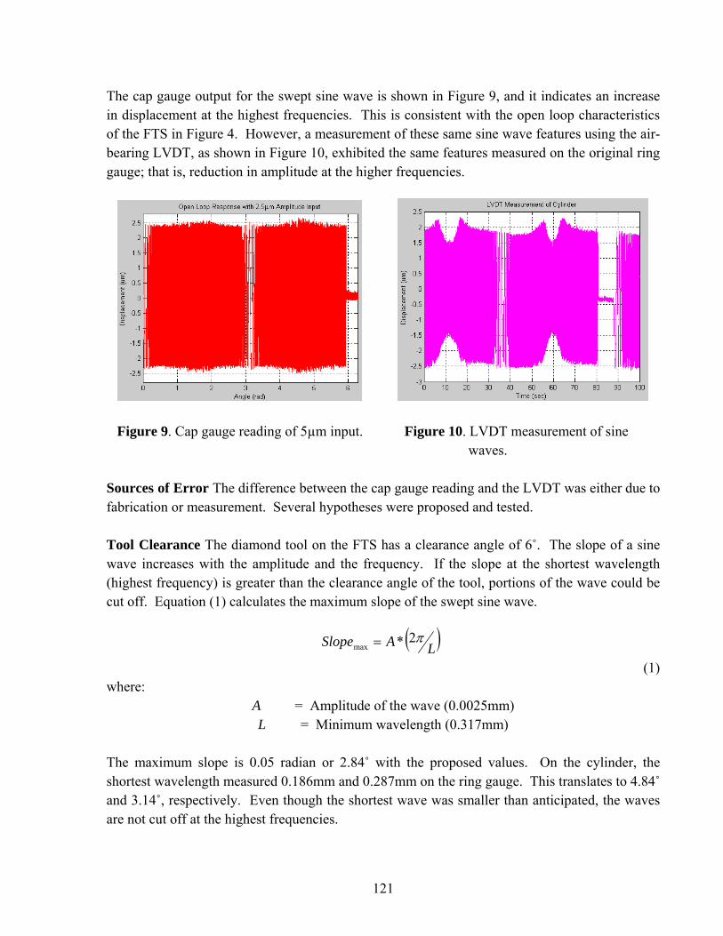
121

The cap gauge output for the swept sine wave is shown in Figure 9, and it indicates an increase in displacement at the highest frequencies. This is consistent with the open loop characteristics of the FTS in Figure 4. However, a measurement of these same sine wave features using the air-bearing LVDT, as shown in Figure 10, exhibited the same features measured on the original ring gauge; that is, reduction in amplitude at the higher frequencies.

Figure 9. Cap gauge reading of 5µm input. Figure 10. LVDT measurement of sine waves. Sources of Error The difference between the cap gauge reading and the LVDT was either due to fabrication or measurement. Several hypotheses were proposed and tested. Tool Clearance The diamond tool on the FTS has a clearance angle of 6˚. The slope of a sine wave increases with the amplitude and the frequency. If the slope at the shortest wavelength (highest frequency) is greater than the clearance angle of the tool, portions of the wave could be cut off. Equation (1) calculates the maximum slope of the swept sine wave.

( )LASlope π2*max = (1)

where: A = Amplitude of the wave (0.0025mm) L = Minimum wavelength (0.317mm)

The maximum slope is 0.05 radian or 2.84˚ with the proposed values. On the cylinder, the shortest wavelength measured 0.186mm and 0.287mm on the ring gauge. This translates to 4.84˚ and 3.14˚, respectively. Even though the shortest wave was smaller than anticipated, the waves are not cut off at the highest frequencies.

122

Probe Tip Diameter The size of the probe used for measurement may also be an issue. There is a maximum probe size that is capable of fitting into each wave. The LVDT used a 1mm diameter probe. Probe compensation equations were applied to the commanded input to determine if and where the probe would not be able to measure [5]. Figure 11 illustrates the areas where the 1mm diameter probe would not fit into the swept sine wave of the cylinder.

Figure 11. Top curve is the expected measurement and lower is the actual LVDT measurement. The probe compensated data showed that the LVDT probe could not measure the valleys of the wave but indicated that all the peaks could be measured. This may be attributed to a shorter spatial wavelength that prevented the probe from fitting into the valley of the wave. The reduction of the peak at the shortest spatial wavelengths may be due to the filtering of the instrument if the probe lost contact with the surface after not being able to properly measure the valleys. The compensation equations do not take into account the speed of measurement and assume exact following of the wave. 6.4 FINAL ARTIFACT After determining the sources of error associated with the trial fabrication of the ring gauge artifact, various changes will be made to the fabrication procedure. Some of those changes will be discussed in the following sections. 6.4.1 MOUNTING CONSIDERATIONS The most significant problem with the overall shape of the ring gauge was due to the distortion of the flat surfaces caused by the amount of torque applied to the bolts to hold the ring during fabrication. The obvious conclusion is to apply less torque to the bolts. The first fabrication included 100 in-lb of torque applied to each bolt. After calculation, it was determined that

123

approximately 5 in-lb would be more appropriate. 5 in-lb of torque on the bolts is equivalent to 100 lbf of a vacuum holding the ring gauge. Small alterations to the ring gauge design could also be made to lessen the distortion influence. Instead of placing counter bores on the opposite sides of one bolt location, the counter bore could be placed on one surface and then the other counter bore applied on the opposite face but rotated 60°. Figure 12 illustrates this idea.

Figure 12. New design of the ring gauge artifact.

It should also be noted that a 45° chamfer is placed on the edge of the counter bore. The chamfer will be used for the resting of steel balls in the horizontal orientation during CMM measurement. Another point of significance is the change in material. As mentioned, the trial ring gauge used Al 6061-T6 whereas the final ring gauge will use 17-4 PH Stainless Steel. The steel is stiffer than the aluminum, which will also decrease the amount of distortion caused by the bolts. 6.4.2 RING TOLERANCES The revised ring gauge design includes a number of tolerances to ensure quality of the artifact. Those specifications were for concentricity, parallelism, perpendicularity, and total run out. Figure 13 shows the specified tolerances.

124

Figure 13. Drawing with tolerance specifications of ring gauge.

Concentricity defines the relationship between one center and another. By choosing the center of the ID, the center of the OD must lie within a 0.001” diameter zone of the ID’s center. Tolerancing the concentricity along with the total run out ensures the uniform thickness of the ring. Total run out is referring to the control of all surface elements around a datum axis. The tolerance uses the datum axis of the ID center. Specifically in terms of the ID and OD, when the surface is rotated 360°, the entire surface must lie within a 0.001” tolerance zone at every position of the placement of the indicator [6]. A parallelism tolerance has been specified to guarantee the hole surface center lies within a 0.001” tolerance zone around the hole center datum axis which is equidistant from the OD and ID of the ring. The perpendicularity tolerance assures that the holes are perpendicular to the top and bottom surfaces of the ring [6]. The 0.001” tolerance values chosen were to ensure that the 0.006” thick Electroless Nickel plating layer is sufficient for machining. 6.5 DATA ANALYSIS Once the final ring gauge has been fabricated, it needs to be measured and the measurement data analyzed. The swept sine wave was generated through Matlab and integrated into a look-up table in the dSPACE model. Some analysis has begun on the perfect swept sine wave. One approach to analyzing the swept sine wave is to apply a Fast Fourier Transform (FFT) to the data set. The swept sine wave measurement is sampled in time, or is in the time domain. By knowing the measurement speed, the sampling rate, and the spatial wavelength of the swept sine wave, the measurement can be placed in the frequency domain. The FFT converts the time

125

domain measurement into the frequency domain. An FFT may be used to determine other frequencies present in a data set that would normally not be apparent in the time sampled measurement. The allure of the swept sine wave is that is it contains a wide range of frequencies. However, this makes the analysis of its FFT more difficult. 6.5.1 DISCRETE FOURIER TRANSFORM (DFT) If a system is defined as f(n) in the time domain and δt is the sampled time with N samples, the DFT converts the time samples to N frequency samples. It creates a complex number with the real value as a cosine component and the imaginary value as a sine component [4]. Equation 2 represents the DFT operation.

⎟⎟⎠

⎞⎜⎜⎝

⎛−⎟

⎠⎞

⎜⎝⎛×= ∑

−

= Nkni

NknnfkF

N

n

ππ 2sin2cos)()(1

0 (2)

where k = 1..N The maximum frequency sampled is equivalent to the reciprocal of the sampling time. The DFT is typically calculated using an FFT algorithm to quicken the calculation [4]. The results of the calculation are used to create a frequency spectrum with magnitude and phase components. If an FFT is performed on a 6 Hz sine wave with an amplitude of 4, the frequency spectrum will indicate the largest magnitude at 6 Hz with a value of 4. The phase is equal to -90° at 6 Hz. Figure 14 demonstrates these attributes.

Figure 14. 6 Hz sine wave (left); FFT frequency response with peak magnitude of 4 and -90° phase at 6 Hz (right). If any phase were added to the above sine wave, the additional phase would be apparent on the phase plot. A phase shift of 45° to the right increases the phase value to -135°.

126

An FFT calculation on a single frequency sine wave is the basis for understanding more complicated signals. Consider a signal with 3 separate sine waves added together as in Figure 15.

Figure 15. Addition of multiple sine waves (left); FFT frequency spectrum (right). The frequency spectrum indicates that the first sine wave is a 1 Hz wave with an amplitude of 2 and a positive additional phase to produce a value of -32.7°. The second wave is 4 Hz, has an amplitude of 1.5 and has also been shifted to the left to give a phase value of -32.7°. The final wave is 8 Hz with an amplitude of 1 and -32.7° of phase. The addition of multiple sine waves produces a classic result, but the placement of single frequency sine waves next to each other creates a different outcome. If a 4 Hz sine wave is concatenated with a 5 Hz sine wave, the frequency spectrum concedes a decrease in amplitude and an increase in phase as shown in Figure 16.

4 Hz 5 Hz4 Hz 5 Hz

Figure 16. Concatenation of two single frequency sine waves (left); FFT frequency spectrum (right).

127

The original amplitude of both waves was 4. However, after the FFT calculation, the peak magnitude is equal to approximately 2.5 at 4.5 Hz. Recall that the magnitude is the square root of the sum of the squares of each component of the complex number. So, at 4 Hz, the magnitude is √4, or 2, and the same is true at 5 Hz. Between 4 and 5 Hz, the magnitude is no longer 4 which alters the value of the peak magnitude found at 4.5 Hz. The phase at 4.5 Hz is also -180° due to the addition of the individual phase values of each wave. The swept sine wave on the ring gauge combines four separate quadrants of the same frequency range. In the first quadrant, the wave begins at a low frequency and progresses to a higher frequency where it is “flipped” over in the second quadrant to return to the starting frequency. This is similar to concatenating several increasing single frequency sine waves, then rotating the complete wave 180° and attaching the rotated wave onto the original wave. Figure 17 illustrates this idea.

Figure 17. Eight single frequency sine waves placed side by side (left); FFT frequency spectrum (right). The sine wave plot is in the time domain but shows where the divisions of the different frequency waves occur. Although the amplitude of each wave is 4, the peak magnitude is smaller for the same reason as was previously described with the two single frequency concatenated waves. The phase remains at -180° for the frequency range because each sine wave repeats itself. For frequencies less than 4 Hz, the phase is zero and for frequencies greater than 7 Hz, the phase accumulates from one frequency to the next. 6.5.2 SWEPT SINE WAVE ANALYSIS The values of the swept sine wave were produced based on a minimum and maximum spatial wavelength. Because the wavelengths can be considered as individual frequencies, an FFT can

128

be performed on the data set. With sampled data, the units on the frequency spectrum plot are in terms of hertz. However, with the generated spatial data, it is more useful to plot the results in terms of wave numbers. The wave number is directly related to the spatial wavelength. Figure 18 represents the FFT of the “perfect” swept sine wave.

Figure 18. FFT of swept sine wave with original amplitude of 5 µm and 20,000 points.

The plot indicates a maximum magnitude of 0.276 µm and 90° phase at a wave number of 34.5; although the magnitude looks relatively constant, each alternating value is zero. The phase is also alternating from +90° to 0° to -90° and vice versa. This is due to the repetition of the individual frequencies in each quadrant; the location of each wavelength is shifted by 90° from the previous location. The FFT of the swept sine wave is difficult to interpret as compared to a single frequency sine wave due to the constantly varying nature of the wavelength. Rather than strictly interpreting the FFT and comparing it to an FFT of an actual measurement, the data analysis may be simplified. A CMM has dynamic characteristics that will influence the overall measurement of the artifact. Since the ideal swept sine wave is known and the CMM will assemble its own data set, the dynamic system may be found using a form of deconvolution [4]. Convolution in the time domain is the multiplication of the swept sine wave and the impulse response of the dynamic system to construct an output that shows the influence of these dynamics. Since the dynamics of a particular CMM are not known, the measurement may be divided by the theoretical wave, the inverse of convolution, or deconvolution. Deconvolution can be calculated in the time domain as well. From the time domain, the dynamics may be converted to the frequency domain to create a bode plot of the system. Figure 19 denotes a theoretical dynamic system.

129

Figure 19. Theoretical second-order dynamic system. If the operator specifies a measurement speed, the speed may be applied to the swept sine wave data and a CMM operating range determined. One measurement speed may correspond to the window illustrated in Figure 19. The operator should expect the actual measurement to look similar to Figure 20.

Figure 20. Simulated swept sine wave measurement. The bode plot (Figure 19) suggested that the magnitude would increase before rapidly decreasing at the natural frequency of the system; the measurement would include some phase from the beginning as well. These attributes are recognizable in the time plot.

130

The transfer function communicates a lot of information about the dynamic system of a particular CMM. However, the operator may not be as concerned with all the details of the system but rather with the amount of error of a single point. It may be necessary to redefine the plot to indicate the possible error within the frequency range of a measurement. 6.6 FUTURE WORK The final aspects of the project will include fabrication of the ring gauge and actual implementation of the data analysis algorithm. The 17-4 PH stainless steel rings have been heat treated and plated with Electroless Nickel. The fabrication control loop along with speed control has been finalized. After fabrication, the artifact may be measured with an LVDT using different speeds to test the theory for data analysis. The last step will be to demonstrate the use of the artifact at Y-12. REFERENCES 1. Wong, A., Folkert, K., and Dow, T. A. Metrology Artifact Development. Precision

Engineering Center Interim Report. October 2003. 2. Weekers, W. G., Schellekens, P. H. J., Compensation for dynamic errors of coordinate

measuring machines. Measurement, 1997, 20 (3), p. 197-209. 3. Cauchick-Miguel, P., King, T., and Davis, J., CMM verification: a survey. Measurement,

1996, 17 (1), p. 1-16. 4. Panusittikorn, W. Error Compensation using Inverse Actuator Dynamics. PhD

Dissertation, NC State University, August 2004. 5. Balkey, M.M., Day, R.D., Batha, S.H., Elliot, N.E., Pierce, T., Sandoval, D.L., Garrard, K.P., and Sohn, A., Production and Metrology of Cylindrical Inertial Confinement Fusion Targets with Sinusoidal Perturbations. Fusion Science and Technology, Vol 45, No 2, p. 107-112, (2004). 6. ANSI Y14.5M – 1982, Dimensioning and Tolerancing. ASME, 1983, New York.

131

7 FAST TOOL SERVO MEASUREMENT

Anthony Wong Undergraduate Student

Thomas A. Dow Professor

Department of Mechanical and Aerospace Engineering

Getting the most from an actuator is the goal of most servo designs. However as the operating frequency increases, gain and phase issues change the actual motion of the actuator from the desired path. Deconvolution techniques seek to identify the dynamics of the actuator and find a modified signal that, when sent through the actuator, will produce the desired path. The deconvolution algorithm requires accurate knowledge of the system dynamics; that is, the gain and phase of the outlet motion compared to the inlet command for an open-loop or a closed loop system. The purpose of this report is to describe methods that were developed to find the dynamics of a Variform fast tool servo (FTS). This piezoelectrically-driven, lever-amplified servo has a range of 300 µm, a small signal bandwidth of 325 Hz and a speed limit of 140 mm/sec. It has a built-in analog control system with an LVDT sensor for position feedback. Because the LVDT measurement was not the true actuator motion, an external sensor (laser interferometer) was introduced to determine the actual motion of the actuator. Fortunately, the relationship between the LVDT and the laser was independent of the operating amplitude and could be integrated into the dynamics as measured by the LVDT. A LabView program was developed to generate the appropriate range of input frequencies and amplitudes, send commands to the Variform, collect the resulting motion data and generate the system dynamics. This method for finding the dynamics of the FTS yields a 1.4% error in magnitude and 2.6% error in phase when compared to the laser measurement. It was also found that excitation at velocities greater than 140mm/s were destructive to the Variform and should be avoided.

132

7.1 INTRODUCTION Machining a precision part requires positioning the tool in the right place at the right time. As the complexity of the part is increased (from spheres to aspheres to freeform surfaces), more axes are necessary and this task becomes more difficult. Actuators, position feedback devices, correction for slide straightness/squareness and control systems (algorithms and high-speed processors) have all been refined to increase the positioning accuracy of these machines. One area that has not received much attention is integration of the actuator dynamics into the command signal. This technique is commonly applied to a wide variety of control systems from manual operation of a crane to actuators for disk drives heads. In the language of system dynamics, the command signal is convoluted with (multiplied by) the system dynamics to produce the actual motion. Conversely, if the desired motion is “deconvoluted” with (divided by) the system dynamics, the required input to get the desired motion will be the result. The PEC is currently developing a deconvolution scheme that will, based on the characteristics of the motion command, automatically determine a new input command to compensate for system dynamics. One of the prerequisite pieces of information to develop this alogirthm is the dynamic characteristic of the system to be controlled. Since this technique is used to modify the command signal, an accurate knowledge of the system characteristics prior to cutting is of utmost importance for the accuracy and precision of the final part shape. For this application the deconvolution algorithm is applied to a commercial actuator, a Variform Fast Tool Servo (FTS), to improve the fidelity during machining of non-rotationally symmetric optical surfaces. The goal of this project is to investigate the dynamic response of the Variform FTS to input commands with different magnitude and frequency and to develop methods to characterize this performance. The characteristics of interest are how the output motion of the FTS changes with frequency and amplitude. The Variform has an internal position sensor, a Linear Variable Differential Transformer (LVDT), which could be used to measure the motion of the Variform and characterize it. However, the internal LVDT is known to have its own dynamics, so the LVDT measurements do not display the FTS dynamics but rather a combination of the two systems. These sensor dynamics mean that the Variform cannot be accurately characterized by using the internal LVDT alone. Also the characterization methods are to be performed by the client, who is assumed to not possess an external measuring system with the range and bandwidth to completely characterize the Variform. 7.2 MEASURING VARIFORM DYNAMICS 7.2.1 STRATEGY Since the output of the LVDT (FTSLVDT) on the Variform does not accurately represent the motion of the tool, the measurement of the tool motion was also made with a separate sensor that

133

could follow the true motion of the tool (FTSTrue). If the relationship between the tool motion as measured by the LVDT and the true motion proved to be repeatable over the range of frequencies of interest, then the Variform system dynamics could be constructed by measuring them with the LVDT and convoluting (multiplying) this result with the ratio of FTSTrue to FTSLVDT as shown in Equation (1).

InputFTS

FTSFTS

InputFTS LVDT

LVDT

TrueTrue *= (1)

This can be written in terms of the transfer function between the true motion of the Variform and that measured by the LVDT in Equation (2) and serves as the basic concept for capturing the dynamics of the Variform.

InputFTSTF

InputFTS LVDT

LVDTLaserTrue */= (2)

7.2.2 EXTERNAL SENSOR A Zygo Axiom 2/20 heterodyne laser interferometer was chosen as the external sensor. In the chosen configuration, the laser measurement system has a range of 0.5 mm, which is greater than the 0.4 mm travel of the Variform. The Axiom also has a maximum velocity measuring capability of 0.9 m/s, which is greater than the maximum velocity of the Variform.

Figure 1: Diagram of Laser Setup (dotted line is horizontal polarized beam and solid line is

vertically polarized)

Figure 1 illustrates the orientation of the laser, interferometer and mirror on the tool mounted in the Variform. A single pass configuration with a focusing lens was used. Two orthogonal

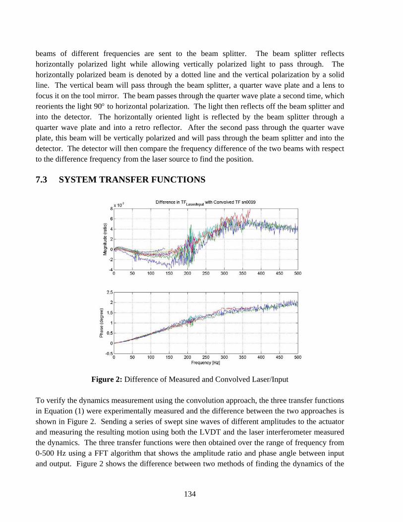
134

beams of different frequencies are sent to the beam splitter. The beam splitter reflects horizontally polarized light while allowing vertically polarized light to pass through. The horizontally polarized beam is denoted by a dotted line and the vertical polarization by a solid line. The vertical beam will pass through the beam splitter, a quarter wave plate and a lens to focus it on the tool mirror. The beam passes through the quarter wave plate a second time, which reorients the light 90° to horizontal polarization. The light then reflects off the beam splitter and into the detector. The horizontally oriented light is reflected by the beam splitter through a quarter wave plate and into a retro reflector. After the second pass through the quarter wave plate, this beam will be vertically polarized and will pass through the beam splitter and into the detector. The detector will then compare the frequency difference of the two beams with respect to the difference frequency from the laser source to find the position. 7.3 SYSTEM TRANSFER FUNCTIONS

Figure 2: Difference of Measured and Convolved Laser/Input

To verify the dynamics measurement using the convolution approach, the three transfer functions in Equation (1) were experimentally measured and the difference between the two approaches is shown in Figure 2. Sending a series of swept sine waves of different amplitudes to the actuator and measuring the resulting motion using both the LVDT and the laser interferometer measured the dynamics. The three transfer functions were then obtained over the range of frequency from 0-500 Hz using a FFT algorithm that shows the amplitude ratio and phase angle between input and output. Figure 2 shows the difference between two methods of finding the dynamics of the

135

actuator motion: first, the transfer function between the laser interferometer and the input, and second, by the convolution (product) of the laser measurement to LVDT measurement with the LVDT measurement to input. Mathematically, Figure 2 shows the following.

[ ]inputLVDTLVDTLaserinputLaser TFTFTFresidual /// *−= (3)

The top graph in Figure 2 indicates that the difference in magnitude is less than 1% using the two measurement techniques and that difference does not vary with amplitude. Therefore, the convolution approach yields excellent results and can be used to find the magnitude of the actuator dynamics using only the internal LVDT motion sensor and using a fixed laser to LVDT transfer function (TFLaser/LVDT). The phase difference is a little more complicated. It has less variation among the different amplitudes and has a nearly linear increase from 0-2 Hz over the 500 Hz range of measurement. In addition, it has a slope change around 300 Hz. A linear phase increase suggests a constant time lag in the convolved transfer function (DA or AD converter time?) but the kink has not been explained. It could be the result of non-linearities in the Variform. The phase error should be a topic for further investigation but is not addressed in this report.

Figure 3: Variform Dynamics (output/input) as measured by laser interferometer

Based on the results above, the mathematical method of convolving transfer functions was confirmed as a viable method of finding the actual dynamics of the Variform. Figure 3 shows the measured Laser/Input transfer function for the system. The small magnitude and phase error shown in Figure 2 will not significantly change this graph. The magnitude variation is 1% and the 2° phase shift from Figure 2 would only be 1.4% out a total phase lag of 144° at 500 Hz.

136

Therefore, the convolution method has been selected to carry the actuator dynamics into the deconvolution method. 7.3.1 VARIFORM DYNAMICS For the convolution method to work an accurate knowledge of the actuator dynamics is needed and those dynamics must be repeatable for the actuators used. If the dynamics are identical for all the Variforms, then only one need be measured; but if variations exist over time or different units, each unit must be measured periodically. Based on previous experiments [1], the motion of the Variform is a strong function of the amplitude. However, the relationship between that motion and the output from the LVDT is independent of the amplitude. To verify this conclusion, Figure 4 shows the amplitude independence of the TFLaser/LVDT. This figure shows the difference between the average value of measurements made at ten different amplitudes (up to 200 µm) and that measured for 1 Volt (20 µm) excitation. The difference between the transfer function at low amplitude and the average is only about 0.5% and will be assumed to have a negligible effect. Accordingly, the average of the TFLaser/LVDT over different amplitudes can be used interchangeably with it measured at any one amplitude.

Figure 4: Magnitude differences between Average and 1 V Amplitude

137

Figure 5 shows the TFLaser/LVDT of three different Variforms (Serial # 0099, 0113, and 0144). The graphs show the average of the transfer function over ten amplitudes. The magnitudes of TFLaser/LVDT for the different Variforms have the same shape but appear to be shifted by a constant. The phase vs frequency is the same for each Variforms.

Figure 5: LVDT Dynamics of 3 Variforms – Serial # 0099, 0113, 0144

The difference in magnitude presents a problem for the convolution method because an external sensor would be needed to find the LVDT dynamics, which negates the goal of this proposed technique. However, the shape similarity can be utilized to minimize this problem. Since the TFLaser/LVDT is independent of amplitude, another sensor with less range and velocity capabilities could be used to find one point on the TFLaser/LVDT. This point could then be used to determine how to appropriately shift the magnitude curve. A readily available sensor such as a Federal gauge or capacitance gauge could be used. If the TFLaser/LVDT were measured at 1 Hz, then the curve could be offset to find the gain for each separate unit. Magnitude Calibration The transfer function TFLaser/LVDT will be set by default to have unity gain at DC and the constant developed by measuring the Variform at low frequency will be used to modify that gain throughout the frequency range. The constant will be found by inputting 1 volt to the Variform

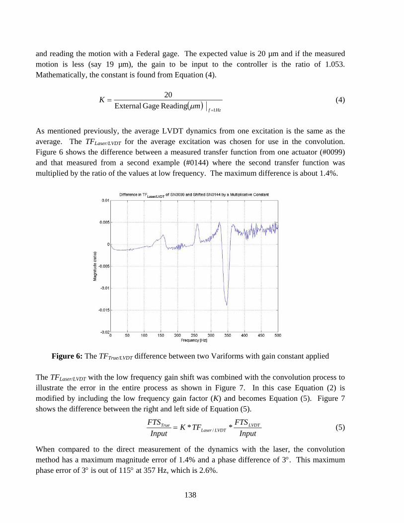
138

and reading the motion with a Federal gage. The expected value is 20 µm and if the measured motion is less (say 19 µm), the gain to be input to the controller is the ratio of 1.053. Mathematically, the constant is found from Equation (4).

( )Hzf

mK

1Reading Gage External20

=

=µ

(4)

As mentioned previously, the average LVDT dynamics from one excitation is the same as the average. The TFLaser/LVDT for the average excitation was chosen for use in the convolution. Figure 6 shows the difference between a measured transfer function from one actuator (#0099) and that measured from a second example (#0144) where the second transfer function was multiplied by the ratio of the values at low frequency. The maximum difference is about 1.4%.

Figure 6: The TFTrue/LVDT difference between two Variforms with gain constant applied

The TFLaser/LVDT with the low frequency gain shift was combined with the convolution process to illustrate the error in the entire process as shown in Figure 7. In this case Equation (2) is modified by including the low frequency gain factor (K) and becomes Equation (5). Figure 7 shows the difference between the right and left side of Equation (5).

InputFTSTFK

InputFTS LVDT

LVDTLaserTrue ** /= (5)

When compared to the direct measurement of the dynamics with the laser, the convolution method has a maximum magnitude error of 1.4% and a phase difference of 3°. This maximum phase error of 3° is out of 115° at 357 Hz, which is 2.6%.

139

Figure 7: Difference between Measured and Convolved then Shifted Laser/Input

7.3.2 VELOCITY LIMIT The Variform actuators have a velocity limit. The manual says that the maximum amplitude up to 100 Hz is 0.008” (200 µm) and from 100 Hz to 200 Hz this value is reduced to 0.004” (100 µm). Experimentally, a sinewave command into the mechanically-amplified piezoelectric actuator begins to distort and turn into a triangle wave when the velocity approaches 140 mm/s. This velocity limit was initially thought to be the limit at which the closed loop controller of the actuator lost accuracy. However, after testing outside this speed, it was determined that high frequency, high amplitude excitations are destructive to the Variform. Two Variforms were able to operate under such taxing conditions, but two others were not and were damaged. Operating at velocities greater than 140 mm/s is possible, but the system may be damaged and such high speeds are not recommended. A limit was placed on the speed to protect the Variform during testing. The required stop frequency is determined by the following equation based on the velocity of a sine wave with a given amplitude1 (A) in mm and frequency (fstop) in Hz.

1 Amplitude is half of the peak-to-valley motion.

140

fstop =1402πA

(6)

CONCLUSION A viable method has been found for characterizing the dynamics of a Variform fast tool servo. Procedures were created to find both the actuator dynamics as measured by the internal LVDT and an external sensor (laser interferometer). The shape of the transfer function between the actual tool motion and that measured by the internal LVDT (TFLaser/LVDT) has been found to be independent of the amplitude and frequency of the excitation. However, the transfer function for a specific example of the Variform may have a different gain. Using an external sensor at low frequency, this gain can be determined and the TFLaser/LVDT compensated. The gain-adjusted transfer function is then convolved with the Variform dynamics as measured by the internal LVDT to give the actual dynamics of the Variform. Using this convolution technique, the error when compared to direct measurement of the dynamics is at most 1.4% in magnitude and 2.6% in phase. The error in the phase is appears to be systematic error and further study of potential sources may reduce the phase error. It has also been observed that damage to the actuator can occur if the velocity limit of 140 mm/s velocity limit is exceeded. The testing procedure was designed to remain below the velocity limit. REFERENCES 1. Panusittikorn, W. Annual Report section 2003 – Lara please fill in details.

141

8 NON-CONTACT TRANSPORTATION USING FLEXURAL ULTRASONIC WAVE

Yin Yanbo

Graduate Student Paul I.Ro Professor

Department of Mechanical & Aerospace Engineering A new non-contact transportation system is being designed at the Precision Engineering Center. The system is based on NFAL (Near-Field Acoustic Levitation) and near boundary streaming. In this report, background knowledge is introduced about applications of NFAL and near boundary streaming. Also, two experiments are set up at the PEC, one is to check the validity of NFA, and the other is to design a non-contact transportation system. Theoretical approaches are then introduced in the report and Ansys software is used to conduct modal, transient analysis.

142

8.1 INTRODUCTION In manufacturing and processing precision products such as compact discs, LCD, LSI and silicon wafers of semiconductors, a non-contact transportation system is indispensable to eliminate tiny defects and scratches. In order to realize such a system, several techniques have been proposed, e.g. gas bearing: transportation with an electromagnetic force or a static electronic force. In these systems, however, several problems must be overcome: (1) Levitated objects are constrained to electrically conductive materials except the gas bearing. (2) In the gas bearing systems, not only an abundance of gas is needed, but also the levitation and transportation mechanism is too complicated and expensive to be conducted. Acoustic levitation can be employed in a non-contact transportation system due to the following advantages: (1) no material is type limited to the levitated object, (2) compact size, (3) free of noise and (4) no demand on large amount of clean gas. This project conducted at the PEC investigated acoustic levitation, designed the experiment setup, proposed governing equations of acoustic levitation and checked the validity. In this report, the experiment setup for the transportation system is described. Y. Hashimoto’s groups on this non-contact transportation conducted a great deal of research. Suspension Mechanism in NFAL was theoretically and experimentally conducted [3][4]. An experimental apparatus was fabricated to measure the transportation speed and transient characteristics [3]. A method was devised that increases the capability of the device to carry large objects by placing vibrating beams in parallel and enlarging the transportation range by placing the vibrating beams in a series [6]. One new experimental system, which consists of multiple ultrasonic actuators, is defined to transport large-size planar objects [7]. Besides non-contact transportation systems, NFAL can also be applied to ultrasonic motor and non-contact linear bearings. 8.1.1 ULTRASONIC MOTOR

Figure 1. Prototype of configuration of ultrasonic motor

143

Figure 1 shows a prototype of the ultrasonic motor, in which two ultrasonic actuators are attached with screws to a cylinder stator made of aluminum. A thin cylindrical rotor is inserted into the stator to make narrow gap between them. Two alternative voltages drive the two actuators with a phase difference of 90, and the distance between the excitation points is three quarters of one wave length of the flexural wave. Therefore a traveling wave in the circumferential direction is excited by superposition of two degenerate standing waves with 90-phase difference. This is commonly used in traditional ultrasonic motors. The resonance frequency of the stator ring is tuned to that of the actuator. Using a non-contact ultrasonic motor, high speeds of 3000rpm can be obtained, which is impossible for a conventional contact ultrasonic motor to achieve.[8]

Figure 2. Revolution speed of rotor vs. stator vibration velocity

As shown in Figure 2, the rotor speed increases linearly with the stator vibration velocity. The revolution speed increases rapidly when exceeding a threshold, which results from the severe turbulence in the flow boundary layer on the rotor surface [8]. The revolution speed and axial rotor stability was fully analyzed and high revolution speed can be obtained. 8.1.2 NON-CONTACT LINEAR BEARING

Figure 3. Prototype of non-contact linear bearing

144

Figure 3 is the prototype of a linear bearing based on Near-Field Acoustic Levitation (NFAL). A beam with an L-shaped cross-section is used for the guide tail and a slider of the same cross- section is levitated by an ultrasonic traveling wave excited along the beam. This provides a small and inexpensive non-contact bearing with immunity against magnetic.

Figure 4. Experiment setup

In Figure 4, the L-shaped beam is excited using a Langevin with a stepped horn at 18kHz, the side length and the wall thickness of the beam are 30mm and 2 mm, respectively. The transducer is mounted diagonally half way from the corner of the L, 45mm from the end of the beam [9].

Figure 5. Thrust versus displacement amplitude

The movement of the levitated slider by two transducers was investigated. The value of the thrust applying on the slider was evaluated by elevating one end of the beam to equalize the thrust and weight of the slider to stop the slider. Figure 5 shows the thrust to the maximum displacement amplitude in the diagonal excitation. The thrust was generated successfully in both directions by changing the driving phase difference.

145

8.2 DETAILS OF THE PROJECT 8.2.1 NEAR FIELD ACOUSTIC LEVITATION (NFAL) The relationship between levitation and input voltage is shown in Figure 6 Here, levitation distance is proportional to the amplitude. The top two lines represent the levitation of two objects with different mass but same mass area ratio.

The Levitation Vs.Input Voltage

15

20

25

30

35

40

45

3 3.5 4 4.5 5 5.5 6

Input Voltage (V)

Levi

tatio

n D

ista

nce(

mic

rom

eter

)

M/A=1.5M/A=1.5M/A=3

Figure 6. Levitation vs. Input Voltage Experiment Set-up The experiment was carried out using the configuration shown in Figure 8. It consists of one rectangular vibration plate (54*40*3 mm) and one mechanical horn connected to the Piezo actuator. The cone horn parameters are shown in Figure 7 and the design sizes are in Table1.

Figure 7. Mechanical Horn design

146

Table 1. Mechanical Cone horn for NFAL

Equations Actual size of horn

2

1

SS

N = 3.8 Relationship between

dimensions

)1(1 xDD α−=

LNN 11

•−

=α

D1=24mm D2=6.316mm

Frequency equation 2

2 )()1(

1)(

KLN

NKLKLtg

−+

=

Length of the horn π

λ KLL •=2

100.083mm

The node position αKKxtg =)( 0 0475.380 =x

mm The Magnification factor

⎥⎦⎤

⎢⎣⎡ •

−−= )sin(11)cos( KL

KLNNKLNM 3.061

Maximum stress position )1(21

1)( MM

M xKxK

Kxtg ααα

αθ −−−

•=+

Shape factor

)cos()cos(2θθαϕ++

•=MKx

KLK

N

Where )(1

Ktg αθ −=

147

Figure 8. Experimental Set-up

The actuator is a Bolted Langevin type Transducer (BLT) manufactured by NTK (Model No. DA2228). The levitated object was placed on the surface of the rectangular plate, which was excited at frequency of 16.8 kHz. A Capacitance Gage and the levitation distance conducted the vibration amplitude measurement by laser displacement meter (Angstrom Resolver Model 101), respectively. Aluminum was chosen as the material of horn and beam because of its excellent acoustic characteristics. Amplitude distribution on the plate Figure 9 shows the distribution of amplitude on the vibration plate. Figure 10(a) is the Chladni’s pattern of vibration and (b) is the mode shape simulated by Ansys. The dissymmetry of the pattern in Figure10 (a) may arise from bad horizontality of the plate.

0

1

2

3

4

5

6

7

8

9

0 5 10 15 20 25 30

0

1

2

3

4

5

6

7

0 2 4 6 8 10 12

(a) Longitude Distribution of Amplitude (b) Sectional Distribution of Amplitude.

Figure 9. Amplitude Distribution on the plate

148

(a) The Chladni’s pattern of vibration mode (b) Mode shape of vibrating plate

Figure 10. Amplitude Distribution and Mode Shape

Analytical Approach

Figure 11. Levitation by Piston Vibration

Levitation by piston vibration Consider an object with a planar bottom levitated by an acoustic standing wave, which is radiated from a piston-like sound source, as shown in Figure 11. The surface of a levitated object is assumed to be rigid plane, and the piston vibrates as

tωξξ cos0= Based on formation derived by B. Chu and R.E. Apfel [2], the radiation pressure is

]2

)2sin(1[

lklk

EKPa

a+><= (1)

Where >< E is the time average energy density and expressed as:

)(sin/4

220

20 lkE aωρ

ξ>=< (2)

Each symbol is defined below:

P, radiation pressure,2

1 γ+=K ,

149

where γ specific heat ratio, for air 4.1=γ , cka /ω= ,

where c sound velocity l Levitation distance 0ξ Vibration amplitude 0ρ Medium density.

Figure 12 shows the derivative results from formation by the two previous authors. When

levitation distance l is small enough to satisfy 1<<lka , the radiation pressure is

2

202

041

lcP

ξργ+

= (3)

Then levitation distance can be derived by making W equal to P as below:

WK

cH2

00

ρξ= (4)

where: W -weight / area of levitated object.

.

Figure 12. Matlab result

(a) Pressure vs. Amplitude (b) Pressure vs. Frequency

(c) Levitation vs. Pressure (d) Levitation vs. Amplitude

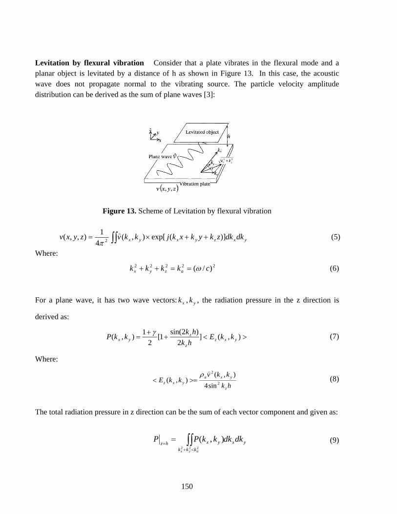
150

Levitation by flexural vibration Consider that a plate vibrates in the flexural mode and a planar object is levitated by a distance of h as shown in Figure 13. In this case, the acoustic wave does not propagate normal to the vibrating source. The particle velocity amplitude distribution can be derived as the sum of plane waves [3]:

Figure 13. Scheme of Levitation by flexural vibration

yxzyxyx dkdkzkykxkjkkvzyxv )](exp[),(4

1),,( 2 ++×= ∫∫)

π (5)

Where: 22222 )/( ckkkk azyx ω==++ (6)

For a plane wave, it has two wave vectors: xk , yk , the radiation pressure in the z direction is

derived as:

><++

= ),(]2

)2sin(1[2

1),( yxzz

zyx kkE

hkhkkkP γ (7)

Where:

hkkkv

kkEz

yxayxz 2

2

sin4),(

),()ρ

>=< (8)

The total radiation pressure in z direction can be the sum of each vector component and given as:

yxkkk

yxhzdkdkkkPP

ayx

∫∫<+

==

222

),( (9)

151

8.2.2 ULTRASONIC TRANSPORTATION Figure 14 shows the schematic diagram of the non-contact transportation system using flexural traveling wave. The traveling wave sound source produces two unidirectional forces on the object in the gap. One is in the normal direction and levitates the object and the other induces the near boundary streaming in the parallel direction. The velocity gradient of the near boundary streaming on the surface of the object produces the viscous force that causes the object to move in a horizontal direction.

Figure 14. Scheme of Transportation System When the beam starts to vibrate, the plate is rapidly levitated and gradually accelerated along the wave propagation direction by the viscous force [3]. The exact governing equation that describes the air velocity gradient and the effect on the transport speed of the object has not been conducted yet. Mechanical Horn Design The vibrating motion generated by the actuator is normally too low for practical use, so it is necessary to magnify this motion, which is the function of a mechanical horn (also called amplitude transformer) that acts as a resonant element in the compression mode. Table 2 shows the design parameters for the combined horn. Figure 15 shows one horn combined with a step and exponential horn, which is being incorporated in the research.

152

Figure 15. Combined Horn

Table 2. Design of Combined Horn

Equation Actual size of

horn The dimension of transition shape

xeDD β−= 1

2

lnL

N=β

221 β−= KK

D1=48mm D2=12mm

Frequency equation 0)2()(ln)(1)( 122

2121

21 =++• KLtgNLKLK

LKtg

The length of the transition shape 22

λ•= HL

where 2221 )(ln)(1 NLKH +=

π

L2=66.895mm

The magnification factor )]sin()[cos( 21221 LKtgLKNM •−= α

where 2

1211)()(

KLNNKLtgtg •−

+=α

4

The node position along the transition shape 2

))(2

( 221

0λαπ

•−= tgLK

Hx 18.577mm

L1,L3 22

3131

λπ

λπ

•=•==KLKLLL 23.374mm

The total length 321 LLLL ++= 113.642mm

153

Beam Design It is simple to design the beam, but it is very important to determine the position of the actuator attached to the beam, because that determines the scale of vibration velocity. Normally, the horn is attached to the beam at a length of 4/λ from the end. Figure 16 and Figure 17 show the beam mode shape of beam.

Mode Shape of the Beam

-2

-1.5

-1

-0.5

0

0.5

1

1.5

2

0 10 20 30 40 50 60

Length (cm)

Mod

e Sh

ape

Phi 30Phi 31

Figure 16. Mode Shape of 30th and 31st Figure 17. Modal Simulation using Ansys

Experiment setup

(a) Top View (b) Side View

Figure 18. Experiment setup

The system shown in Figure 18 consists of one beam (400*50.8*3.175mm) and two Langevin type Transducers (BLT) manufactured by NTK (Model No. DA4427), which are attached to the beam at a length of 4/λ from the end of the beam. When there are phase angles of 90º difference, the traveling wave is produced and changes the phase difference between the two transducers. Thus, changing the transportation direction. Since there is no support force across the width of

154

the vibrating beam, the levitated object is not stable and slides off easily during transportation. It is necessary to make appropriate vibration distributions across the plate in order to transport a levitated object stably. One traditional but effective method to make both ends thinner can obtain the desirable vibration distribution to prevent the plate falling off the beam. The system is excited at a frequency of 25.6 KHz, which makes the most desirable traveling wave on the beam. When a flat plate (r=36.1mm mass=4g) is put on the vibrating beam, the plate is suddenly levitated and then gradually accelerated to a certain speed due to the near boundary streaming produced by the traveling wave. Due to the oscillation along the width direction, it is difficult to get the position using a Laser displace meter. The author uses a simple but effective method, Web Cam, to capture the motion, and then utilizes Matlab to derive the position versus time data. The flow chart of derivation is shown in Figure 19. The video is divided into frames and on each frame the plate is marked with darker dot in the center, therefore the position can be obtained by calculating the intensity. Figure 20 shows the divided frames, from which the marked dot can be seen in the figure.

Figure 19. Derivation Flow Chart

155

Figure 20. Divided Frames

Figure 21. Position versus Time

Figure 21 shows the position versus time for the first three curves, which have the same phase angle, and the rest as a result of inversing the phase angle. From the figure, it can be seen that the motion of the plate is gradually accelerated and then moves at a constant speed. The velocity of the plate is about 11 cm/s. By making the phase angle of two transducers 0, the plate can stay stable on the beam with tiny oscillation amplitude. In order to obtain a precise stop-go control, a close-loop control is desired.

Marked Dot

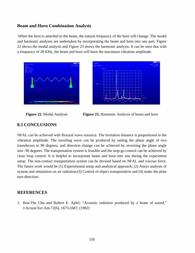
156

Beam and Horn Combination Analysis When the horn is attached to the beam, the natural frequency of the horn will change. The modal and harmonic analyses are undertaken by incorporating the beam and horn into one part. Figure 22 shows the modal analysis and Figure 23 shows the harmonic analysis. It can be seen that with a frequency of 28 KHz, the beam and horn will have the maximum vibration amplitude.

Figure 22. Modal Analysis Figure 23. Harmonic Analysis of beam and horn 8.3 CONCLUSIONS NFAL can be achieved with flexural wave resource. The levitation distance is proportional to the vibration amplitude. The traveling wave can be produced by setting the phase angle of two transducers to 90 degrees, and direction change can be achieved by reversing the phase angle into -90 degrees. The transportation system is feasible and the stop-go control can be achieved by close loop control. It is helpful to incorporate beam and horn into one during the experiment setup. The non-contact transportation system can be devised based on NFAL and viscous force. The future work would be (1) Experimental setup and analytical approach; (2) Ansys analysis of system and simulation on air radiation;(3) Control of object transportation and (4) make the plate turn direction. REFERENCES 1. Boa-The Chu and Robert E. Apfel, “Acoustic radiation produced by a beam of sound,”

J.Acoust.Soc.Am.72(6), 1673-1687, (1982)

157

2. Hideyuki Nomura, Tomoo Kamakura and Kazuhisha Matsuda, ”Theoretical and experimental examination of near-field acoustic levitation,” J.Acoust.Soc.Am. 111(4),1578-1583,(2002).

3. Ide, T., J.Friend, K.Nakamura and S.Ueha,”a Non-contact linear bearing by ultrasonic

levitation,” WCU 2003,Paris.2003. 4. Junhui Hu,Kentaro Nakamura and Sadayuki Ueha,”An analysis of a noncontact ultrasonic

motor with an ultrasonically levitated rotor,” Ultrasonics 35 ,459-467, 1997. 5. Lin Zhongmao, The Principle and Design of Ultrasonic Amplitude Transformer,Science

Press,Beijing,1987.[In Chinese]. 6. Sadayuki Ueha, Yoshiki Hashimoto and Yoshikazu Koike,”Non-contact transportation using

near-field acoustic levitation ,” Ultrasonics 38 ,26-32,(2000). 7. Takafumi Amano, Yoshikazu Koike, Kentaro Nakamura, Sadayuki Ueha and Yoshiki

Hashimoto,”A multi-tranducer near field acoustic levitation system for noncontact transportation of large-sized planar objects,” Jpn.J.Apple.Phys., vol 39, 2982-2985,2000.

8. Yoshikau Koike,Sadayuki Ueha,Atsushi Okonogi, Takafumi Amano and Kentaro

Nakamura,”Suspension Mechanism in Near field acoustic levitation phenomenon,” IEEE ULTRASONICS SYMPOSIUM,671-674,(2000)

9. Yoshiki Hashimoto, Yoshikazu Koike and Sadayuki Ueha, “Near-field acoustic levitation of

planar specimens using flexural vibration,” J.Acoust.Soc.Am.100(4),2057-2061,(1996). 10. Yoshiki Hashimoto, Yoshikazu Koike and Sadayuki Ueha,”Magnification of transportation

range using Non-Contact acoustic Levitation by connecting vibrating plates,” Jpn.J.Apple.Phys., vol 36, 3140-3145,1997

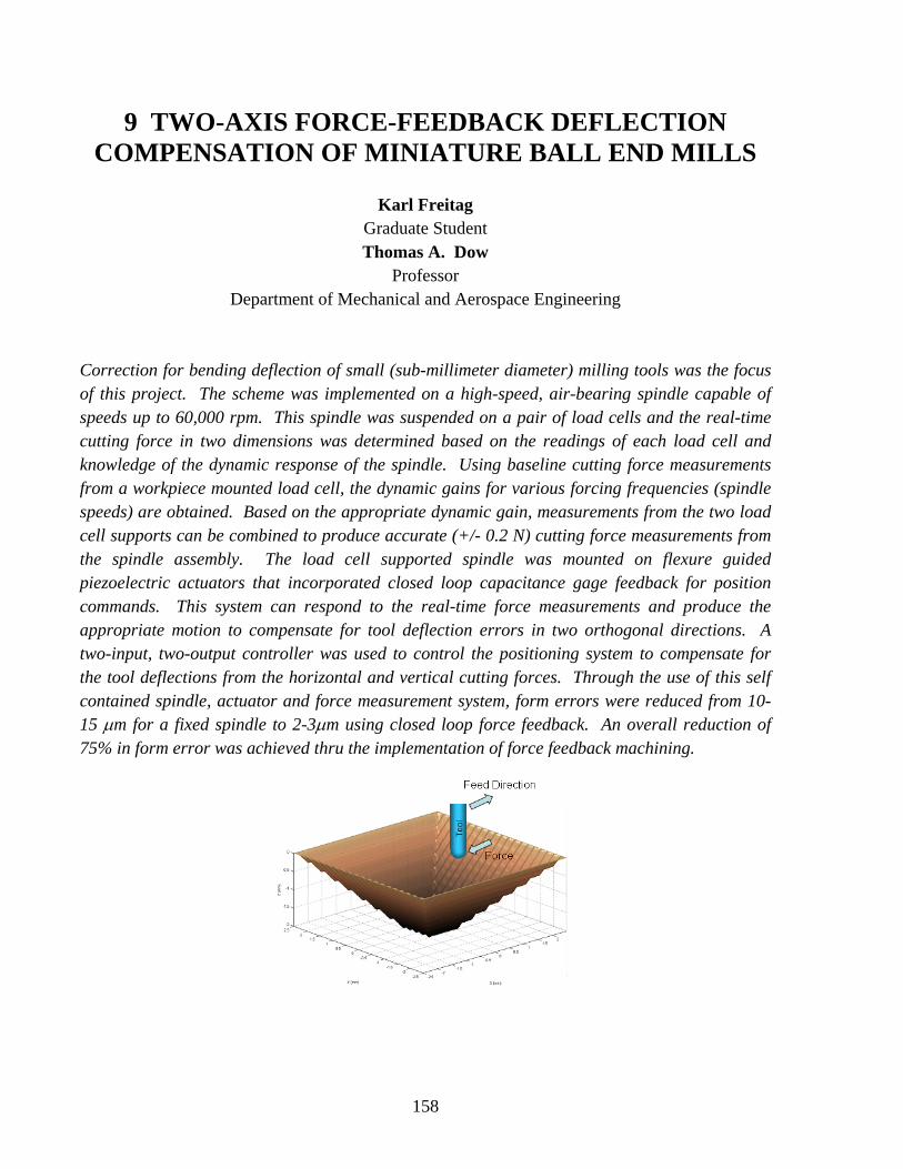
158

9 TWO-AXIS FORCE-FEEDBACK DEFLECTION COMPENSATION OF MINIATURE BALL END MILLS

Karl Freitag Graduate Student Thomas A. Dow

Professor Department of Mechanical and Aerospace Engineering

Correction for bending deflection of small (sub-millimeter diameter) milling tools was the focus of this project. The scheme was implemented on a high-speed, air-bearing spindle capable of speeds up to 60,000 rpm. This spindle was suspended on a pair of load cells and the real-time cutting force in two dimensions was determined based on the readings of each load cell and knowledge of the dynamic response of the spindle. Using baseline cutting force measurements from a workpiece mounted load cell, the dynamic gains for various forcing frequencies (spindle speeds) are obtained. Based on the appropriate dynamic gain, measurements from the two load cell supports can be combined to produce accurate (+/- 0.2 N) cutting force measurements from the spindle assembly. The load cell supported spindle was mounted on flexure guided piezoelectric actuators that incorporated closed loop capacitance gage feedback for position commands. This system can respond to the real-time force measurements and produce the appropriate motion to compensate for tool deflection errors in two orthogonal directions. A two-input, two-output controller was used to control the positioning system to compensate for the tool deflections from the horizontal and vertical cutting forces. Through the use of this self contained spindle, actuator and force measurement system, form errors were reduced from 10-15 µm for a fixed spindle to 2-3µm using closed loop force feedback. An overall reduction of 75% in form error was achieved thru the implementation of force feedback machining.

159

9.1 INTRODUCTION Fabricating micrometer features on hard steel injection molding dies is a difficult problem. To reach the regions of interest, the diameter of these milling tools are often limited to a millimeter or less and lengths of 4 to 7 mm are often required. The tools required for such machining are (Diameters < 1.0 mm) termed miniature tools and are the focus of this research. These tools are available in several different shank lengths to accommodate various applications and die geometries. Figure 1 contains a photograph of the 0.8 mm diameter miniature ball end mills used. The tools are made of tungsten carbide with a titanium aluminum carbide coating. Although the tool material is very strong, the thin geometry of these tools results in low tool stiffness (0.2 N/µm and less), which becomes a significant factor when machining heat treated steels. Deflections of these tools under low (10N) cutting forces can produce part errors of 50 µm with a 4.0mm shank tool. The primary goal of this research is to reduce tool deflection errors to ± 2 µm, through the use of force-feedback machining.

Figure 1. Miniature Ball End Mills on left with close-up of ball end on right This report is the culmination of several projects on this topic beginning with open loop control using path correction [1,2], followed up by one-dimensional correction with a load cell under the part [3] and a second one-dimensional correction scheme with the sensor and correction scheme on the spindle [4]. Each of these techniques developed new approaches to correction of the deflection of the miniature tools. However, each had its drawbacks related to the amount of effort needed to implement the control scheme or the limited correction capability available. The technique described here uses a self-contained spindle that can measure the forces on the tool in two directions and a correction scheme that compensates for the deflection of the tool caused by those forces.

160

9.2 DESCRIPTION OF APPARATUS The apparatus consists of three parts: the force measurement system, the actuation system and the control system. The force measurement system uses a pair of 3-axis load cells to sense the force in 2 orthogonal directions and the actuation system uses a pair of piezoelectric actuators to move the spindle to compensate for the tool deflection caused by the cutting forces. The controller takes the information from the force system and sends commands to the actuation system with position feedback from a pair of capacitance gages to acknowledge the motion. 9.2.1 FORCE MEASUREMENT SYSTEM When measuring the cutting forces from the spindle assembly, the locations of the load cells are very important. They should not be located inside the force loop between the actuators and ground. The reaction forces from the piezoelectric actuators must have a ground to push against that are free from the load cells. If the load cells are located in this force loop, the actuation forces of the piezoelectric actuators will be measured by the load cells and interfere with cutting force measurements. For this reason, the load cells are located as close to the measurement source as possible, situated below the spindle block and above the piezo actuators as shown in Figure 2.

Figure 2. Force Measuring Spindle Design (Center of Gravity at ⊗)

In this spindle based measurement system, two load cells are used so that all reaction forces between the spindle and its ground are captured. They are equally spaced about the center of gravity of the spindle to cancel the effects of in-phase or out-of-phase spindle vibrations as needed in the later force signal processing. Using the results obtained by increasing spindle speed during cutting, the frequency response of the spindle assembly can be obtained in the X, Y and Z directions. From this data, a look-up table is generated in Simulink (Matlab) to cross reference the spindle speed (forcing frequency)

161

with the appropriate dynamic magnification factor. In essence, the magnitude portion of the transfer function is measured and then assembled into a lookup table for implementation on the A/D data acquisition system. The block diagram for this force measurement algorithm is illustrated in Figure 3.

Figure 3. Force Measurement Block Diagram

Once the spindle speed has been determined, the dynamic magnification factor is extracted from the look-up tables whose data was generated in the previous experiment. Three independent look up tables are used to account for the X, Y, and Z directions. The Simulink model for this subsystem is located below in Figure 4.

Figure 4. Simulink Dynamic Magnification Factor Subsystem

162

The results of this force measurement technique produce forces measured on the spindle equivalent to the forces measured on the work piece during a cut. Figure 5 is a comparison between the force measured on the work piece and the force measured on the spindle assembly as well as the output from the force measurement algorithm of Figure 4. The results clearly show that the spindle mounted force sensors give the same force measurement as a sensor mounted to the lightweight part.

Figure 5. Comparison of the cutting forces measured on the work piece and spindle

9.2.2 ACTUATION SYSTEM The actuation system used piezoelectric actuators as the prime mover and flexures to control the motion. Piezoelectric actuators are crystalline materials that respond with strain upon application of an electric field. Flexures are compliant mechanisms [5] designed to utilize linear elastic deformation as a means to produce fine motion or precise forces. In its simplest form, a flexure element consists of two rigid bodies interconnected with a compliant element. Flexures are advantageous for producing precision motion since they are free from stiction, backlash, and friction present in rotary or linear bearings. The absence of stick-slip conditions results in smooth precise motion. This smooth motion is based on linear elastic deformation and the elasticity theory. For small displacements, there will be a linear relationship between applied force and displacement. A number of different actuation strategies were investigated including linear, rotary and stacked axes. One of the difficulties is avoiding crosstalk between the axes so that correction in each direction can be accomplished based on the force components measured by the load cells. The best design was to create two flexure axes at the appropriate locations to produce the desired

163

displacement. The resulting two-axis flexure design is illustrated below in Figure 6. The dotted lines illustrate the two flexure axes of rotation for this design.

Figure 6. Two Axis Flexure Design Figure 7 shows how this design moves when vertical actuation is desired. The actuators are located at the arrows and both elongate to move the spindle, which is on the bottom plate. The deflection occurs in the pivot at the end away from the tool but in line (vertically) with the tool.

Figure 7. Vertical Actuation using the two piezoelectric actuators together The horizontal actuation uses the two actuators in a push-pull mode where one is lifting one side of the bottom plate and the second is pulling it down as illustrated in Figure 8. Since the piezoelectric actuators cannot supply a tensile force, the push and pull is accomplished by preloading the actuators such that the preload force will provide the pull to move that side of the bottom plate down. A preload force of 800N is applied directly above each stack thru the compression of a Belleville washer. This preload is applied directly above the piezo actuators to

Pivot

164

avoid application of a bending moment to the load cell plate which can effect the measurement of the cutting force from the load cells.

Figure 8. Horizontal Actuation is accomplished by twisting the bottom plate

The two axis force feedback actuator was designed to produce the tool error correction of 40 µm in the horizontal and vertical direction guided by flexures with displacement feedback from a pair of capacitance gages. The force is measured with a pair of 3-axis load cells that connect the spindle to the actuation platform. A top view of the complete apparatus is shown in Figure 9.

Figure 9. Force Measurement Platform with spindle and back flexures visible

Pivot

165

9.3 MULTIVARIABLE CONTROL The force feedback spindle actuator is a two-input two-output system where the displacement at each piezo stack contributes to both the horizontal and vertical tool position. Control of the actuator is achieved through decoupling of the horizontal and vertical dynamics. Proportional Integral (PI) control is used to control the horizontal and vertical systems separately and then recombined to solve for the individual voltage to each piezo. The horizontal controller produces the differential voltage between the two piezos while the vertical controller produces a sum. The command following of the two-axis actuator was evaluated with an 8µm square profile. The square motion profile below in Figure 10 (Left) was positioned in a total time of 500ms. The complete force feedback control algorithm is shown below in Figure 10 (Right) where the horizontal and vertical tool forces are first measured to produce a desired horizontal and vertical tool position. The two axis controller then positions the tool to the desired position using capacitance gage closed loop feedback. Step response for a horizontal and vertical 2µm step are displayed below in Figure 11.

+

-Controller

-

+

C1

C2

Xm

Ym

Tool Position Equations

2212

2111

CbCaY

CbCaX

⋅+⋅=

⋅+⋅=

FX

FYtoolk1

Tool ComplianceMeasuredForce

toolk1

Tool Compliance

Cap Gages

MeasuredForce

Y

X

r1

r2

e1

e2

u1

u2

PZT1

PZT2

Actu

ator

Figure 10. Command following, Tool position (µm), Force-Feedback Block Diagram (Right)

Figure 11. Horizontal Step Response (Left), Vertical Step Response (Right)

166

9.4 EXPERIMENTAL VERIFICATION To study the potential of this force feedback technique, the spindle with force measuring and error correction system was added to the Nanoform 600 diamond turning machine, as shown in Figure 12. This spindle was mounted on the y-axis of the machine and that axis was used to move the tool in the vertical direction. The y-axis was in turn mounted on the z-axis that changed the depth of cut. The part was mounted on the x-axis, which moved the part left to right. In this way, a three dimensional part could be fabricated and the error corrected in the plane of the part, that is, the x (horizontal) and y (vertical) directions.

Workpiece

Force-FeedbackSpindle Actuator

Figure 12. Force-Feedback Spindle Actuator mounted on Diamond Turning Machine

9.4.1 PART PROFILES 5mm Hemisphere To test the two-axis force feedback actuator, a 5mm diameter hemisphere was milled into a flat workpiece as shown in Figure 13. To machine the 5 mm diameter hemisphere, a raster cut sequence was used. In a raster cut sequence, one axis is used to increment position sequentially while the other rasters back and forth performing the contouring of the part.

167

Figure 13. Workpiece with 5 mm Diameter Hemisphere

The Y-axis on the DTM is used to increment the vertical position between each step while the X and Z-axes, which have higher resolution encoders, are used to perform the contouring of the sphere. The X,Y,and Z machine tool paths for the raster cut 5mm diameter hemisphere is shown in Figure 14.

Figure 14. X,Y,Z Tool Path for 5mm Raster Cut Hemisphere

To machine the 5mm diameter hemisphere, successive hemispheres of increasing radii are machined until the final diameter of 5mm is reached. The radius of the hemisphere is incremented by 100 µm for each hemisphere sequence using a crossfeed (∆Y) of 50 µm. This results in a total of 100 passes to machine the 5 mm diameter hemisphere.

168

In the initial raster cut sequence, a portion of the tool deflection errors from each pass were cut away by the following pass in the opposite direction because the tool has a different deflection in that direction. To avoid removal of errors from the previous pass and facilitate part measurement, a consistent tool feed direction was used; that is, the machining was always in the same direction. Tool Radius Compensation The tools used in the force-feedback machining experiments were ball end mills with a tool radius of 400 µm. To obtain the desired final part geometry, the tool path was corrected to account for the radius of the tool. To machine a hemisphere with a ball end mill, the compensated tool path forms a smaller diameter hemisphere located inside the desired geometry offset by the tool radius. The geometric relationship between the compensated tool path and the desired geometry is shown in Figure 15. To machine a 5 mm diameter hemisphere using a 0.8 mm diameter ball end mill, the tool path radius is adjusted to (2.5 mm-0.4 mm) = 2.1 mm to account for the 400 µm tool radius.

ToolRadius = 400 µm

Tool Path

Material Removed

Figure 15. Tool Radius Compensation for Hemisphere Cut

Part Measurement The first measurements of the machined hemisphere were made using an air bearing LVDT probe on the Nanoform to scan along the surface of the part. Due to the steep slope at the edge of the hemisphere, the probe needed to be positioned at an angle to avoid interference with the probe tip. The part to be measured was mounted to the Nanoform spindle to rotate around the hemisphere axis while recording spiral surface data from the LVDT probe. Due to the form error of the hemisphere, centering the hemisphere on the Nanoform axis was not feasible since there was no way to discern the form error from part runout. Measurement of the 5 mm hemisphere (Figure ) was attempted on the Talysurf profilometer by tilting the part to increase probe clearance. Interference of the Talysurf probe near the hemisphere walls dominated the measurement, making most of the data void. As a result, it was

169

difficult to accurately predict the sphere radius from the limited angular range of data. The best fit radius of the hemisphere center was 2.474 mm resulting in a radial error of 26 µm short from the desired radius of 2.5 mm.

Figure 16. 5mm Hemisphere (right), Talysurf Profile (left)

The Talysurf data in Figure 16 contains three horizontal scans across the hemisphere at different locations and the shank of the probe interfering with the spherical surface at each end. To compare the surface error of two hemispheres, the two scans must also run through the same points. A new part with less steep walls was suggested to facilitate measurement.

Four Sided Frustum The geometry and form error of a four sided frustum can be measured on the Talysurf profilometer without the probe interference or critical alignment needed with the hemisphere. A four-sided frustum is the geometry that is obtained by removing the top of a four-sided pyramid (Figure 17Figure ).

Figure 17. Four-Sided Frustum, 6061 Aluminum

The geometry of the frustum is easier to measure since the slope of the walls can be set to avoid interference with the Talysurf probe. The center square of the frustum also makes this profile less sensitive to probe alignment since the probe does not have to pass thru the exact center. The

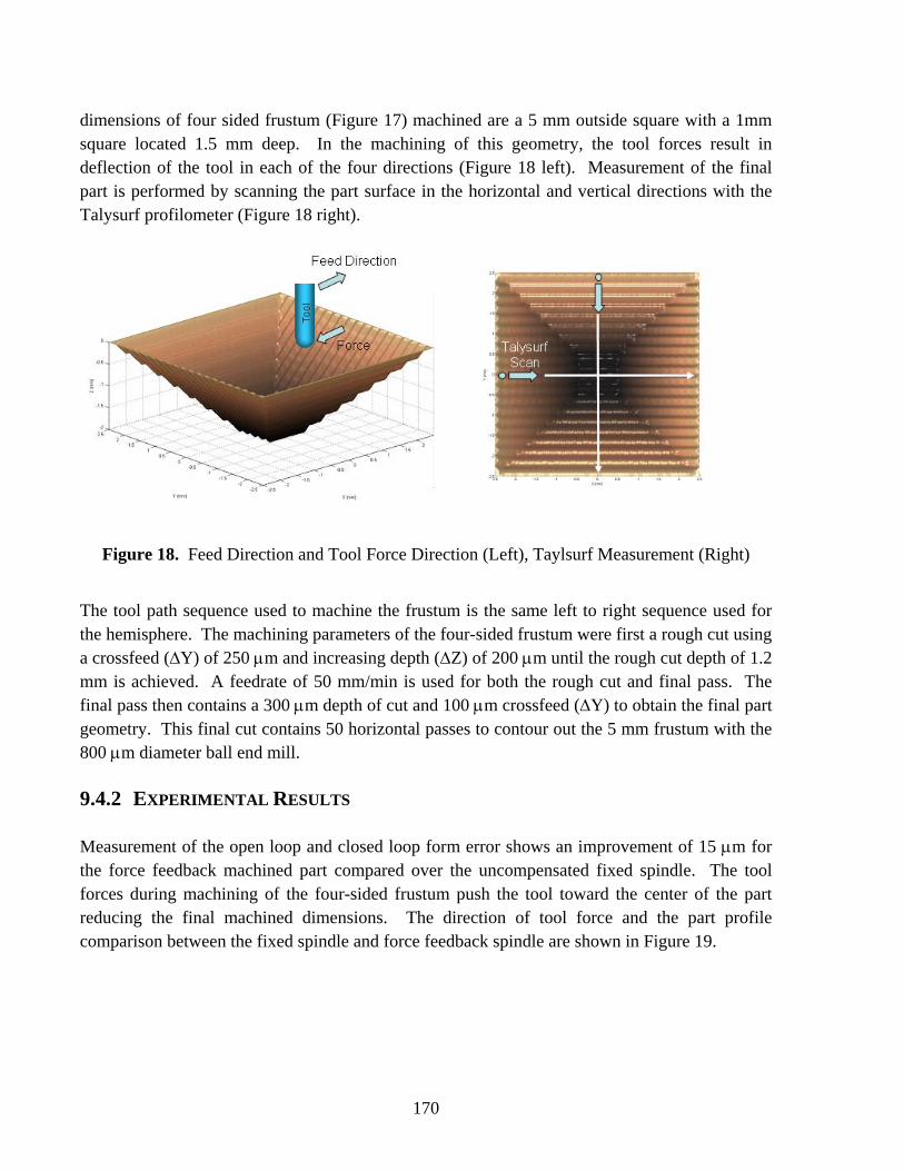
170

dimensions of four sided frustum (Figure 17) machined are a 5 mm outside square with a 1mm square located 1.5 mm deep. In the machining of this geometry, the tool forces result in deflection of the tool in each of the four directions (Figure 18 left). Measurement of the final part is performed by scanning the part surface in the horizontal and vertical directions with the Talysurf profilometer (Figure 18 right).

Figure 18. Feed Direction and Tool Force Direction (Left), Taylsurf Measurement (Right)

The tool path sequence used to machine the frustum is the same left to right sequence used for the hemisphere. The machining parameters of the four-sided frustum were first a rough cut using a crossfeed (∆Y) of 250 µm and increasing depth (∆Z) of 200 µm until the rough cut depth of 1.2 mm is achieved. A feedrate of 50 mm/min is used for both the rough cut and final pass. The final pass then contains a 300 µm depth of cut and 100 µm crossfeed (∆Y) to obtain the final part geometry. This final cut contains 50 horizontal passes to contour out the 5 mm frustum with the 800 µm diameter ball end mill. 9.4.2 EXPERIMENTAL RESULTS Measurement of the open loop and closed loop form error shows an improvement of 15 µm for the force feedback machined part compared over the uncompensated fixed spindle. The tool forces during machining of the four-sided frustum push the tool toward the center of the part reducing the final machined dimensions. The direction of tool force and the part profile comparison between the fixed spindle and force feedback spindle are shown in Figure 19.

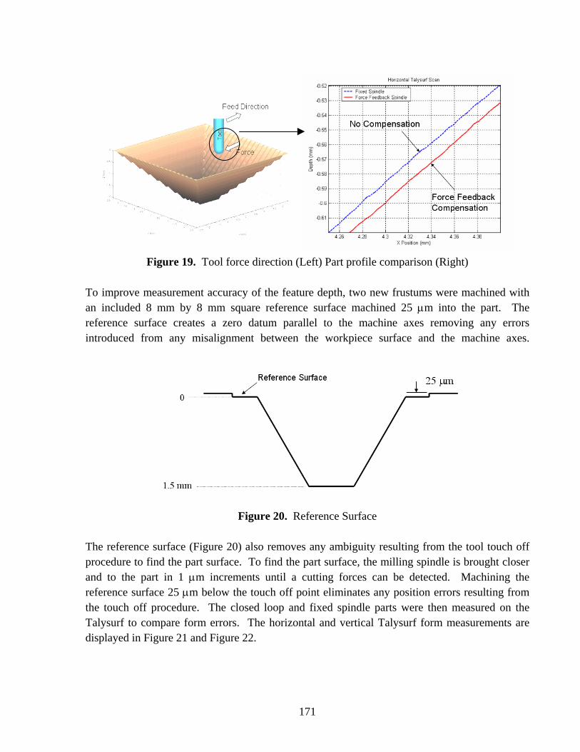
171

Figure 19. Tool force direction (Left) Part profile comparison (Right)

To improve measurement accuracy of the feature depth, two new frustums were machined with an included 8 mm by 8 mm square reference surface machined 25 µm into the part. The reference surface creates a zero datum parallel to the machine axes removing any errors introduced from any misalignment between the workpiece surface and the machine axes.

Figure 20. Reference Surface

The reference surface (Figure 20) also removes any ambiguity resulting from the tool touch off procedure to find the part surface. To find the part surface, the milling spindle is brought closer and to the part in 1 µm increments until a cutting forces can be detected. Machining the reference surface 25 µm below the touch off point eliminates any position errors resulting from the touch off procedure. The closed loop and fixed spindle parts were then measured on the Talysurf to compare form errors. The horizontal and vertical Talysurf form measurements are displayed in Figure 21 and Figure 22.

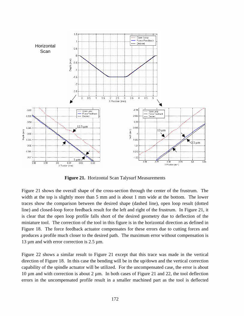
172

Figure 21. Horizontal Scan Talysurf Measurements

Figure 21 shows the overall shape of the cross-section through the center of the frustrum. The width at the top is slightly more than 5 mm and is about 1 mm wide at the bottom. The lower traces show the comparison between the desired shape (dashed line), open loop result (dotted line) and closed-loop force feedback result for the left and right of the frustrum. In Figure 21, it is clear that the open loop profile falls short of the desired geometry due to deflection of the miniature tool. The correction of the tool in this figure is in the horizontal direction as defined in Figure 18. The force feedback actuator compensates for these errors due to cutting forces and produces a profile much closer to the desired path. The maximum error without compensation is 13 µm and with error correction is 2.5 µm. Figure 22 shows a similar result to Figure 21 except that this trace was made in the vertical direction of Figure 18. In this case the bending will be in the up/down and the vertical correction capability of the spindle actuator will be utilized. For the uncompensated case, the error is about 10 µm and with correction is about 2 µm. In both cases of Figure 21 and 22, the tool deflection errors in the uncompensated profile result in a smaller machined part as the tool is deflected

Horizontal Scan

12.5 µm

1 µm

13 µm

2.5 µm

173

away from the desired location. The overall form error is reduced from 10-15 µm to 2-3 µm using the force feedback actuator, attaining a 75% reduction of error.

Figure 22. Vertical Scan Talysurf Measurements

9.5 CONCLUSIONS AND FUTURE WORK Real time cutting force measurement can be obtained from the machining spindle using two load cell supports, once the dynamic response of the spindle is incorporated. Using baseline cutting force measurements from a workpiece mounted load cell, the dynamic gains for various forcing frequencies (spindle speeds) are obtained. Using the appropriate dynamic gain, measurements from the two load cell supports can be combined to produce accurate (+/- 0.2 N) cutting force measurements from the spindle assembly.

Vertical Scan

10 µm 10 µm

2 µm

1 µm

174

Using flexure guided piezoelectric actuators incorporating closed loop capacitance gage feedback, two axis tool positioning is produced to compensate for tool deflection errors as a result of the real time cutting forces. A two-input two-output controller is used to control the two axis tool positioning, which corresponds to the tool deflection and results from the horizontal and vertical cutting forces. Through the use of this self contained spindle actuator and force measurement system, form errors were reduced from 10-15 µm for a fixed spindle to 2-3µm using closed loop force feedback. An overall reduction of 75% in form error was achieved thru the implementation of force feedback machining. The mechanical design of the 2-axis system allows the machining force in each direction to be independently measured and the tool end positioned to compensate for the resulting deflection. Two 3-axis load cells are used to measure the force and the correction is made with two piezoelectric actuators that use capacitance gages for position feedback. Techniques for capturing the peak force, using that force along with the tool compliance to create a positioning error, comparing that error with the cap gage readings and sending the filtered commands to the actuators have been developed and demonstrated. Two machined features are described: a 5 mm radius hemisphere and a 5 mm wide 4-sided frustrum. Each surface was machined using a raster scan technique and the magnitude and direction of the machining forces were measured and tool deflection compensated. Error in final part geometry due to tool deflection was reduced by 15µm through the implementation of force feedback compensation.

.

REFERENCES 1. Dow, T., Miller E., Garrard K., Sohn A., Wright, T. “Compensation of Tool Force in Small

Diameter End Mills,” ASPE Proceedings, Vol. 20, pp. 546-550 and to be published in Precision Engineering in 2003

2. Miller, E., “Deflection Prediction and Error Correction of High Speed Miniature Milling

Tools,” MS Thesis, North Carolina State University, 2000. 3. Hood, D, “Force Feedback Control of Tool Deflection in Miniature Ball End Milling,” MS

Thesis, North Carolina State University, 2003. 4. Clayton , S. , “Force Modeling and Deflection Compensation of Miniature Ball End Mills,”

MS Thesis, North Carolina State University, 2003.

175

5. Smith, S., Flexures: Elements of Elastic Mechanisms, Gordon and Breach Science Publishers, 2000

6. Lobontiu, N., Compliant Mechanisms: Design of Flexure Hinges, CRC Press, 2003. 7. Drescher, J. D., “Tool Force Measurement in Diamond Turning,” MS Thesis, North Carolina

State University, 1989. 8. Arcona, C., “Tool Force, Chip Formation and Surface Finish in Diamond Turning,” Ph.D.

Dissertation, North Carolina State University, 1996. 9. Minor, P., “Tool Wear and Tool Forces in High Speed Machining of Aluminum,” MS

Thesis, North Carolina State University, 1998. 10. Altintas, Y., Manufacturing Automation: Metal Cutting Mechanics, Machine Tool

Vibrations, and CNC Design, Cambridge University Press, 2000.

176

FAC

UL

TY

, ST

AFF

, AN

D S

TU

DE

NT

S O

F T

HE

PR

EC

ISIO

N E

NG

INE

ER

ING

CE

NT

ER

St

andi

ng (L

to R

): N

. Wan

na, L

. Lam

onds

, R. W

oods

ide,

N. B

uesc

her,

R. S

catte

rgoo

d, T

. Dow

and

K. G

arra

rd

Sitti

ng:

(L to

R):

D. B

rehl

, K. F

olke

rt, A

. Soh

n, B

. Bro

cato

, T. K

enne

dy a

nd L

. Mas

ters

St

uden

ts N

ot P

ictu

red:

K. F

reita

g, S

. Hal

bur,

W. P

anus

ittik

orn,

T. R

anda

ll, a

nd Y

. Yin

Fa

culty

Not

Pic

ture

d: G

. Buc

kner

, J. E

isch

en, P

. Ro,

P. R

usse

ll an

d D

. You

den

177

178

179

FACULTY THOMAS A. DOW Director, Precision Engineering Center Professor, Department of Mechanical and Aerospace Engineering BS, Mechanical Engineering, Virginia Polytechnical Institute, 1966 MS, Engineering Design, Case Institute of Technology, 1968 PhD, Mechanical Engineering, Northwestern University, 1972 After receiving his PhD degree from Northwestern University in 1972, Dr. Dow joined the Tribology Section of Battelle Columbus Laboratories and worked there for ten years. His research interests were in the areas of friction and wear and included studies on a wide variety of topics from lubrication of cold-rolling mills using oil-in-water emulsions to wet braking effectiveness of bicycle brakes to elastohydrodynamic lubricant film generation in ball and roller bearings. He developed experimental apparatuses, established analytical models, and corroborated those analyses with experimental measurements. Dr. Dow joined the faculty at North Carolina State University in 1982 and was instrumental in developing the academic and research program in precision engineering. His current research interests include the design of precision machining systems, real-time control, and metrology. He was one of the founders of the American Society for Precision Engineering and currently acts as the Executive Director.

180

GREGORY D. BUCKNER Assistant Professor, Department of Mechanical and Aerospace Engineering BS, Mechanical Engineering, Louisiana State University, 1986 MS, Mechanical Engineering, Virginia Polytechnic Institute, 1987 PhD, Mechanical Engineering, University of Texas at Austin, 1996 After receiving his PhD degree from the University of Texas at Austin in 1996, Dr. Buckner joined the University of Texas Center for Electromechanics (UT-CEM), where he served as a research engineer until 1999. His research at UT-CEM focused on the design and implementation of advanced controllers for electromechanical systems. Applications included self-learning control systems for active vehicle suspensions, magnetic bearings for flywheel systems, and manufacturing processes. Dr. Buckner joined the faculty at North Carolina State University in 1999 as an Assistant Professor of Mechanical and Aerospace Engineering. Dr. Buckner's research and teaching interests focus on the design and control of electromechanical systems, with an emphasis on self-learning algorithms. Current research topics include electromechanical actuators for system identification of milling processes, and magnetic bearings for flywheel and milling applications.

181

JEFFREY W. EISCHEN Associate Professor Department of Mechanical and Aerospace Engineering BS, Mechanical Engineering, UCLA, 1978 MS, Mechanical Engineering, Stanford University, 1981 PhD, Mechanical Engineering, Stanford University, 1986 Dr. Eischen has been with N.C. State since 1986 and his research areas of interest include computational solid mechanics, elasticity, fracture mechanics and structural dynamics. Dr. Eischen worked with Failure Analysis Associates from June 1978 - June 1986 as a Mechanical Engineer. His primary responsibilities included analysis and prevention of industrial equipment failures.

182

PAUL I. RO Associate Professor Mechanical and Aerospace Engineering Department BS, Mechanical Engineering, University of Minnesota, 1982 MS, Mechanical Engineering, Massachusetts Institute of Technology, 1985 PhD, Mechanical Engineering, Massachusetts Institute of Technology, 1989 Dr. Ro joined the faculty of North Carolina State University in January 1989, as an Assistant Professor in the Mechanical & Aerospace Engineering Department. He became an Associate Professor in July 1994. Dr. Ro has developed two graduate courses in the department (multivariable Control and Robotics) and has taught undergraduate Automatic Control and Dynamics courses. His research covers a wide range of controls and various applications of control theories in the following three areas: Precision Engineering, Robotics and Intelligent Vehicle Control. In precision engineering, Dr. Ro’s research concentrates on the characterization and control of microdynamic behaviors of precision slide systems (ball-screw, traction drive, piezo-electric drive, electrostatic drives and magnetic servo levitated drive) to enhance their nano-motion capabilities, development of advanced control schemes and experimental verifications to improve diamond turning process using force and position sensory feedbacks, design of a long-range fast tool servo system using magnetic servo levitated actuators, and active control of precision slide vibration using piezo-electric drives. In robotics, some of the on-going projects include design and implementation of free-floating non-holonomic space robot and a planar passive-joint robot for fuel consumption minimization, neural-fuzzy hybrid scheme for mobile robot path planning, and two-arm coordinated motion control for fixtureless assembly. In intelligent vehicle control, on-going projects include nonlinear tire model identification by Artificial Neural Network, hybrid neural-sliding mode control of 4 Wheel steering for robust handling, semi-active suspension control using energy based Fuzzy Logic scheme, and others.

183

PHILLIP E. RUSSELL Professor Department of Materials Science and Engineering BS, Physics, Appalachian State University, 1975 MS, Physics, West Virginia University, 1977 PhD, Materials Science and Engineering, University of Florida, 1982 After graduate work at the University of Florida, Dr. Russell joined the Solar Energy Research Institute (a DOE lab) in Golden Co. in 1980. There he developed a photovoltic materials and device characterization laboratory with emphasis on electron and ion beam analytical instrumentation. After three years at SERI, Dr. Russell joined JEOL, Inc. in Boston, Massachusetts, an electron optical instrumentation company where he led the technical and application groups. One of his major projects was the development of an electron beam based integrated circuit metrology system. He was also involved in the development and application of focused ion beam systems and electron beam lithography systems, as well as numerous analytical instrumentation projects. On joining North Carolina State University, Dr. Russell took on the role of Director of the Analytical Instrumentation Facility and has established graduate level courses in electron optics and electron optical instrumentation techniques. He was awarded the NSF Presidential Young Investigator Award in 1987. His research at NCSU and the Precision Engineering Center are in the areas of Scanned Probe Microscopy, Focused Ion Beam Technology, Scanning Electron Microscopy, Lithography metrology and beam testing of integrated circuits.

184

RONALD O. SCATTERGOOD Professor Materials Science and Engineering Department BS, Metallurgical Engineering, Lehigh University, 1961 MS, Metallurgy, Massachusetts Institute of Technology, 1963 PhD, Metallurgy, Massachusetts Institute of Technology, 1968 R.O. Scattergood is a Professor in the Department of Materials Science and Engineering. He received BS degrees in Mining Engineering and Metallurgical Engineering from Lehigh University. His MS and PhD degrees were obtained in Metallurgy from M.I.T. In 1968 he became a member of the basic research staff in the Materials Science Division at the Argonne National Laboratory. In 1981, he joined the faculty as a Professor of Materials Engineering at North Carolina State University. Professor Scattergood's major research interests have been focused on the mechanical behavior of solids. He has worked in the areas of strengthening mechanisms in solids, continuum theory of defects, radiation effects, wear and fracture processes in ceramics, and precision engineering with emphasis on machining processes. He has expertise in both analytical and computer modeling as well as in mechanical testing methods and microscopy. He has published over 140 technical papers, books and reports.

185

DAVID YOUDEN Technical Associate, Eastman Kodak Company Adjunct Lecturer, Department of Mechanical and Aerospace Engineering ASME, Central New England College, Worcester, MA, 1965 Prior to joining Eastman Kodak's Manufacturing Systems Technology Division in 1997, Mr. Youden was Research and Development Manager at Rank Pneumo, a division of Rank Taylor Hobson Inc. for ten years. Before that, he was Director of Engineering at the Cone Blanchard Machine Company. He has also worked at Ocean Systems, Inc. of Reston, Virginia and the Heald Machine Company, a division of Cincinnati Milacron. During his professional career, Mr. Youden has been granted numerous patents in the field of machine tools, and he has published and presented technical papers on the design and testing of ultra-precision machine tools in the US, Japan, and Germany. Mr. Youden graduated from Central New England College and attended Worcester Polytechnic Institute and Clark University. He is a charter member of the American Society for Precision Engineering.

186

STAFF KENNETH P. GARRARD Research Assistant Precision Engineering Center BS, Computer Science, North Carolina State University, 1979 MS, Computer Studies, North Carolina State University, 1983 As a full-time research assistant, Mr. Garrard is studying the design of systems software that supports the development of high-speed real-time applications for special purpose multiprocessor computer systems. He has several years experience in academia and industry designing and implementing real-time systems. As a Precision Engineering Center staff member, Mr. Garrard's current activities include the design and implementation of software for Diamond Turning Machine and Fast Tool Servo controller projects. LARA MASTERS Administrative Assistant Precision Engineering Center BA, Religious Studies, College of Charleston, 2000 MPA Candidate, North Carolina State University Mrs. Masters became a member of the PEC Staff in August 2003. Previously she served as public policy intern at North Carolina Center for Nonprofits in Raleigh, NC, and as an event planner at Capital City Club in Raleigh, NC. Mrs. Masters brings to the Center her knowledge of nonprofit management and public policy and provides the overall administrative support for the Center.

187

ALEXANDER SOHN Research Assistant/Lecturer Precision Engineering Center B.S., Physics, University of Texas at Arlington, 1992 M.S., Physics, University of Texas at Arlington, 1994 Mr. Sohn joined the Precision Engineering Center in August, 1997 as a member of the technical staff. His current research interests range from machine design and metrology to the design and fabrication of nonimaging optics. Mr. Sohn's varied research activities began in microwave optics and atomic physics as a student at the University of Texas at Arlington and later progressed to precision machine design, design and fabrication of plastic optics as well as automation and machine vision at Fresnel Technologies, Inc. in Fort Worth, Texas.

188

GRADUATE STUDENTS DURING 2004 DAVID BREHL’s extensive industrial career includes a range of design, development, and project engineering roles with AERCO International, BOC Gases, and Babcock & Wilcox. A deepening interest in design of integrated electromechanical systems, along with a desire to focus his career on technology development, led him to pursue a PhD in Mechanical Engineering at NC State; this follows a recent Master’s in ME program at Stevens Institute of Technology (Hoboken, NJ). He joined the PEC in August 2004. BRETT BROCATO interned at Fort James Paper and TRW Vehicle Safety Systems prior to graduating from the University of Alabama in 1999 with his bachelor's degree is in Mechanical Engineering with a minor in the Computer Based Honors Program. Before enrolling in the NC State master's program, he worked for Bell Helicopter and Corning Optical Fiber. NATHAN BUESCHER was born and raised in Raleigh, NC. He received his BS in Mechanical Engineering as well as a Minor in Mathematics from NC State University in May 2003. He began work with the PEC in August 2003. Some of his prior work experience includes Stantec Consulting, Inc. and Joel Wittkamp Design. KARALYN FOLKERT is originally from Zeeland, MI. She received her BS in Mechanical Engineering from Western Michigan University. While completing her undergraduate workk, she participated in Tribology research and was published. Her senior design project involved the design of a range interlock system for a heavy-duty, 10-speed transmission. She began her work at the PEC in the fall of 2003. KARL FREITAG graduated from Clarkson University in 1995 with a BS in Mechanical Engineering. After graduation he went to work in the automotive industry for New Venture Gear’s Transfer Case Division in Syracse, NY. At NVG, he worked as a product engineer and worked on the transfer case design for the 1998 Dodge Durango. After NVG, Karl has been working for the past 7 years as a Senior Engineer in Optical Fiber Manufacturing for Corning, Inc. in Wilmington, NC. Karl completed his master’s degree in fall 2004 and is currently employed at Northrop Grumman in Baltimore, Maryland. SIMON HALBUR comes from La Crosse, WI. He completed his undergraduate work at Loras College in Dubuque, IA where he obtained a B.S. in Electromechanical Engineering and a minor in Mathematics. During his studies he performed research for the University of Texas at Arlington on the development of a wireless sensor network. His work at PEC began in early 2004 and he graduated that fall.

189

TIM KENNEDY was born and raised in Chapel Hill, NC. Tim received his BS from NCSU in May 2004. Before working at the PEC, he work at the Analytical Instrumentation Facility for two years as an undergraduate research assistant. He started working with the PEC August 2004. WITOON PANUSITTIKORN began his graduate study at NCSU in Industrial Engineering and earned his MIE in 1998. Before graduating with his MSME in May 2001, Witoon developed a nonlinear control algorithm to manipulate a magnetic-free material handling system, using ultrasonic vibration. He applied his knowledge of the nonlinear controller on a magnetic hysteresis in a magnetostrictive transducer and completed this project in the first year of his tenure as a Ph.D. student in Mechanical Engineering. Currently, he is developing an open-loop control algorithm for precision manufacturing at he PEC. The technique uses digital signal processing to correct amplitude and phase response of a fast tool servo. Witoon completed his Ph.D. in 2004 and returned to his home country of Thailand. TRAVIS RANDALL received his BS in Ceramic Engineering from Alfred University in May 2002. Originally from Ann Arbor, MI, Travis spent most of his life in upstate New York. He started working with the PEC and NC State in August 2002. Prior to arriving at NC State, he worked for NYS Department of Transportation and Alcoa Chemical. His research at the PEC entails the study of scribing mechanics in single crystal silicon. Travis completed his M.S. in 2004. YANBO YIN received his BS and ME in Precision Instrument and Mechanology from Tsinghua University Beijing in 2000 and 2003 respectively. For his undergraduate thesis, he joined the micro-mechanical lab with experimental research on Micro-jet. For his master’s degree,Yin developed a computer aided system on wireless communication on base station distribution. Currently, he is pursing his Ph.D. degree in Mechanical Engineering under guidance of Dr.Ro. His research involves Non-contact object transportation using ultrasonic.

190

UNDERGRADUATE STUDENTS DURING 2004 ANTHONY WONG was raised in Virginia Beach, VA. He first came to NC State in fall 2001 to begin his undergraduate study of Mechanical Engineering. Before working as a Research Assistant at the PEC, Anthony previously did research in structural health monitoring and structure of CuA1C14.

191

GRADUATES OF THE PRECISION ENGINEERING CENTER

Student Degree Date Company/Location Jeffrey Abler PhD December 1994 ETEC Systems, Inc.

Tucson, AZ

William Allen PhD December 1994 North Carolina State Univ. Raleigh, NC

Kelly Allred MS June 1988

Christopher Arcona PhD May 1993

Norton Worcester, MA

Bradford Austin MS June 2000 IBM Corporation Fishkill, NY

Markus Bauer PhD December 2001 SCYNEXIS Chemistry & Automation, Inc. Research Triangle Park, NC

Tom Bifano PhD June 1988 Boston University Boston, MA

Scott Blackley MS May 1990 Motorola Austin, TX

Peter Blake PhD December 1988 NASA Goddard Greenbelt, MD

Mark Cagle MS June 1986 NASA-Langley Norfolk, VA

John Carroll PhD January 1986 Cummins Engine Co. Columbus, IN

Matthew Cerniway MS October 2001 Naval Surface Warfare Ctr West Bethesda, MD

Damon Christenbury MS June 1985 Michelin Tire Co. Spartanburg, SC

Stuart Clayton MS May 2003 Naval Depot Cherry Point

192

James Cuttino PhD December 1994

UNC – Charlotte Charlotte, NC

Bob Day PhD July 1998 Los Alamos National Lab Los Alamos, NM

Joseph Drescher PhD May 1992 Pratt & Whitney East Hartford, CT

William Enloe MS December 1988 ITT Roanoke, VA

Karl Falter MS December 1989 Eastman Kodak Company Raleigh, NC

Peter Falter PhD May 1990 Lockheed-Martin Orlando, Florida

John Fasick MS May 1998 Kodak Rochester, NY

Steven Fawcett PhD June 1991 MicroE Natick, MA

Andre Fredette PhD May 1993 IBM Research Triangle Park, NC

Karl Freitag MS August 2004 Northrop Grumman Baltimore, MD

David Gill PhD August 2002 Sandia National Laboratories Albuquerque, NM

Jim Gleeson MS June 1986 Battelle Columbus Labs Columbus, OH

Mary Smith Golding MS May 1990 Harris Corporation Melbourne, FL

David Grigg PhD August 1992 Zygo Corporation Middlefield, CT

Hector Gutierrez PhD October 1997 Florida Inst. Of Tech. Melbourne, FL.

193

Christian Haeuber MS December 1996

Harris Corporation Melbourne, FL

Simon Halbur MS December 2004

Matias Heinrich MS July 2001 Vistakon Jacksonville, FL

Gary Hiatt

PhD May 1992 Caterpiller Zebulon, NC

David Hood MS May 2003

Peter Hubbel MS December 1991 Delco Electronics Kokomo, IN

Konrad Jarausch PhD

December 1999

Intel Corporation San Jose, CA

Bradley Jared

PhD December 1999 3M Cincinnati, OH

David Kametz MS August 2002 Naval Air Warfare Center Aircraft Division Patuxent River, MD

Jerry Kannel PhD June 1986 Battelle Columbus Labs Columbus, OH

Byron Knight MS May 1990 Harris Corporation Melbourne, FL

Mark Landy MS June 1986 Battelle Columbus Labs Columbus, OH

Mike Loewenthal

MS December 1988 SVG Norwalk, CT

Michael Long

PhD June 2000 Eastman Kodak Rochester, NY

Bryan Love MS May 2001 Virginia Tech

Michael Hung-Tai Luh MS June 1989 Proctor and Gamble Cincinnati, OH

194

Dan Luttrell MS 1987 Luttrell, Inc. New Boston, NH

Edward Marino MS September 1999 Pratt Whitney Hartford, CT

Edward Miller

MS December 2000 General Electric Greenville, SC

Michele Miller PhD December 1994 Michigan Tech. University Houghton, MI

Paul Minor MS September 1998 Hartford, CT

Gary Mitchum MS June 1987 Harris Corporation Melbourne, FL

Charles Mooney MS December 1994

JEOL Peabody, MA

Patrick Morrissey MS May 2003

Larry Mosley PhD June 1987 Intel Corporation Chandler, AZ

Patrick Moyer PhD May 1993 UNC-Charlotte Charlotte, NC

Nobuhiko Negishi MS August 2003

Ayodele Oyewole MS October 1997 Pratt & Whitney East Hartford, CT

Hakan Ozisik PhD December 1989

Witoon Panusittikorn PhD December 2004 Thailand

John Pellerin MS May 1990 Sematech Austin, TX

Travis Randall MS August 2004 MBA student NCSU

Ganesh Rao MS December 1994 Oak Ridge National Lab Oak Ridge, TN

195

John Richards MS September 1997 Intel Corporation San Jose, CA

Walter Rosenberger MS May 1993 The East Group Kinston, NC

Alex Ruxton MS December 1996 Pratt &Whitney Palm Beach, Florida

Anthony Santavy

MS August 1996

Ford Dearborn, MI

Keith Sharp PhD May 1998 Morgan Crucible Dunn, NC

Gordon Shedd PhD March 1991

Wonbo Shim PhD May 2000 Seagate Inc. Oklahoma City, OK

Robert Skolnick MS September 1997 San Diego, CA

Denise Skroch MS May 1989 IBM Corporation Raleigh, NC

Elizabeth Smith MS April 1989

Stanley Smith PhD May 1993

Ronald Sparks PhD May 1991 Alcoa Corporation Pittsburg, PA

Brent Stancil MS December 1996 Harris Corporation Melbourne, FL

Gene Storz MS May 1994

Anand Tanikella PhD August 1996 Norton Industrial Ceramics Northboro, MA

Donna Thaus MS May 1996 Northern Telecom Research Triangle Park, NC

John Thornton

MS December 1993 Digital Instruments Santa Barbara, CA

196

Michael Tidwell

MS December 1991

John Tyner MS June 1995 Naval Depot Cherry Point

Tao Wu PhD December 2003 Gave birth to Evan Wu Zhang July 31, 2003.

197

ACADEMIC PROGRAM Problems and limitations associated with precision manufacturing can originate in the machine, the process, or the material. In fact, most problems will probably be caused by a combination of these factors. Therefore, improvement of current processes and development of new manufacturing methods will require knowledge of a multi-disciplinary array of subjects. The educational goal of the Precision Engineering Center is to develop an academic program which will educate scientists and engineers in metrology, control, materials, and the manufacturing methods of precision engineering. The graduate students involved in the Precision Engineering Center have an annual stipend as research assistants. They can take up to 3 classes each semester while spending about 20 hours per week on their research projects. These students also work in the Center full-time during the summer months. The Precision Engineering Center began in 1982 with an emphasis on the mechanical engineering problems associated with precision engineering. As a result, the original academic program proposed was biased toward courses related to mechanical design and analysis. However, as the research program has developed, the need for complementary research in sensors, materials, and computers has become obvious. A graduate student capable of making valuable contributions in the computer area, for example, will require a significantly different academic program than in mechanical engineering. For this reason, the Center faculty has set a core curriculum and each student in the program is required to take at least 3 of these core courses. The remainder of the courses for the MS or the PhD degree are determined by the university or department requirements and the faculty committee of the student. The required courses are: • MAE 545 Metrology in Precision Manufacturing • PY 516 Physical Optics • MAT 700 Modern Concepts in Materials Science • CSC (ECE) 714 Real Time Computer Systems

198

PhD DEGREE PROGRAM The PhD program in Precision Engineering has been set up as a multi-disciplinary program, drawing upon courses throughout the University to provide background and expertise for the students. It should contain required courses to insure solid grounding in the fundamentals plus electives to prepare the student in his area of specialization. Because Precision Engineering is concerned with an integrated manufacturing process, students interested in computer control, materials, machine structure, and measurement and actuation systems are involved in the program. Student research projects include the wide variety of topics addressed in this report. Each student's thesis should have an experimental component because Precision Engineering is basically a hands-on technology.

MS DEGREE PROGRAM The Master of Science degree will have a higher percentage of application courses than the PhD degree. The emphasis will be to develop the foundation for involvement in precision engineering research and development. A total of 30 credits including 6 credits for the MS thesis is required. The thesis, while less comprehensive than the PhD dissertation, will be directed at important problems in Precision Engineering. Typically the MS program will take four semesters plus one summer.

UNDERGRADUATE PROGRAM The undergraduate degree broadly prepares an engineering student for industrial activities ranging from product design and engineering sales to production implementation. Because a large share of engineers only have the BS degree, these will be the people who must implement the new technology developed in research programs like the Precision Engineering Center. Therefore, a way must be found to acquaint engineers at the BS level with the techniques, problems, and potential of precision manufacturing. In most undergraduate degree programs only limited time is available for technical electives. However, these electives offer the student the opportunity to expand his knowledge in many different directions. Beginning graduate courses (such as metrology) can be used as undergraduate electives.

199

Undergraduate projects and summer employment have also been utilized to include undergraduate students into the research program of the Center. During the 1998-1999 academic year, four undergraduate students in Mechanical Engineering were involved various projects at the PEC.

STUDY PLANS Study plans for several example students are given below both for the MS and the PhD degree. Because of the breadth of the field and the wide range of thesis topics, few if any study plans will be exactly the same. The plan will depend upon the student's background, his interests, his thesis topic, the department, and the chairman and members of his committee. PhD PROGRAM IN MECHANICAL ENGINEERING Major Courses: • MAE 740 Advanced Machine Design I • MAE 741 Advanced Machine Design II • MAE 706 Heat Transfer Theory & Applications • MAE 713 Principles of Structural Vibration • MAE 760 Computational Fluid Mechanics and Heat Transfer • MAE 545 Metrology in Precision Manufacturing • MAE 715 Nonlinear Vibrations • MAE 716 Random Vibration • MAE 714 Analytical Methods in Structural Vibration • MAE 742 Mechanical Design for Automated Assembly • MAE 895 Doctoral Dissertation Research Minor Courses: • MA 511 Advanced Calculus I • MA 775 Mathematical Methods in the Physical Sciences I • CSC 780 Numerical Analysis II • PY 516 Physical Optics • ECE 716 System Control Engineering • MAT 700 Modern Concepts in Materials Science • ECE 726 Advanced Feedback Control • ECE 764 Digital Image Processing

200

PhD PROGRAM IN MATERIALS ENGINEERING Major Courses: • MAT 710 Elements of Crystallography and Diffraction • MAT 700 Modern Concepts in Materials Science • MAT 556 Composite Materials • MAT 715 Transmission Electron Microscopy • MAT 795 Defect Analysis/Advanced Materials Experiments • MAT 753 Advanced Mechanical Properties of Materials • MAT 712 Scanning Electron Microscopy • MAT 895 Doctoral Dissertation Research Minor Courses: • PY 414 Electromagnetism I • ST 502 Experimental Statistics for Engineers I • MAE 740 Advanced Machine Design I • MAE 741 Advanced Machine Design II • MAE 545 Metrology in Precision Manufacturing • PY 516 Physical Optics • MA 401 Applied Differential Equations II PhD PROGRAM IN ME (FOR STUDENT WITH MS DEGREE) • ECE 716 System Control Engineering • ECE 791 Gate Array Design • MAT 700 Modern Concepts in Materials Science • PY 516 Physical Optics • MA 502 Advanced Mathematics for Engineers and Scientists II • MA 775 Mathematical Methods in the Physical Sciences I • MA 780 Numerical Analysis II • MAE 732 Fundamentals of Metal Machining Theory • MAE 740 Advanced Machine Design I • MAE 741 Advanced Machine Design II • MAE 545 Metrology in Precision Manufacturing • MAE 716 Random Vibration

201

MS PROGRAM FOR ME STUDENT • MAE 713 Principles of Structural Vibration • MAE 740 Advanced Machine Design I • MAE 545 Metrology in Precision Manufacturing • MAT 700 Modern Concepts in Materials Science • PY 516 Physical Optics • MA 501 Advanced Math for Engineers and Scientists I • MA 502 Advanced Math for Engineers and Scientists II • MAE 695 Master's Thesis Research

MS PROGRAM FOR COMPUTER SCIENCE STUDENT • CSC 501 Operating Systems Principles • CSC 506 Architecture of Parallel Computers • CSC 512 Compiler Construction • ECE 521 Computer Design and Technology • CSC 715 Concurrent Software Systems • MAE 545 Metrology for Precision Manufacturing • MAE 789 Digital Control Systems • ECE 764 Digital Image Processing

MS PROGRAM FOR MATERIALS SCIENCE STUDENT • MAT 700 Modern Concepts in Material Science • MAT 710 Elements of Crystallography and Diffraction • MAT 715 Transmission Electron Microscopy • MAT 712 Scanning Electron Microscopy • MAT 722 Advanced Scanning Electron Microscopy and Surface Analysis • MAE 545 Metrology for Precision Manufacturing • PY 516 Physical Optics • ECE 738 IC Technology and Fabrication • MAT 695 Master's Thesis Research

202

MS PROGRAM FOR PHYSICS STUDENT • PY 516 Physical Optics • PY 552 Introduction to Structure of Solids I • PY 753 Introduction to Structure of Solids II • PY 781 Quantum Mechanics I • PY 782 Quantum Mechanics II • PY 783 Advanced Classical Mechanics • PY 785 Advanced Electricity and Magnetism I • PY 786 Advanced Electricity and Magnetism II • MAT 700 Modern Concepts in Material Science • MAE 545 Metrology for Precision Manufacturing • PY 695 Master's Thesis Research

SHORT COURSES AND TV COURSES Six graduate level courses: Scanning Electron Microscopy (MAT 712), Advanced SEM Surface Analysis (MAT 722), Modern Concepts in Material Science (MAT 700), Mechanical Properties of Materials (MAT 705), and Metrology (MAE 545) have been offered as video courses nationwide via National Technological University. In a typical year, approximately 120 students from industry and national laboratories participate in these courses. Future plans call for a MS program in Precision Engineering to be offered via the television network.

TECHNICAL REPORTS Volume 1 - 1983 December 1983 136 pages Volume 2 - 1984 January 1985 168 pages Volume 3 - 1985 January 1986 294 pages Volume 4 - 1986 January 1987 255 pages Volume 5 - 1987 December 1987 336 pages Volume 6 - 1988 December 1988 362 pages Volume 7 - 1989 March 1990 357 pages Volume 8 - 1990 March 1991 385 pages Volume 9 - 1991 March 1992 382 pages Volume 10 - 1992 March 1993 289 pages Volume 11 - 1993 March 1994 316 pages Volume 12 - 1994 March 1995 268 pages Volume 13 - 1995 January 1996 251 pages

203

Volume 14 - 1996 January 1997 232 pages Volume 15 - 1997 January 1998 298 pages Volume 16 – 1998 January 1999 258 pages Volume 17 – 1999 January 2000 232 pages Volume 18 – 2000 January 2001 274 pages Volume 19 – 2001 January 2002 201 pages Volume 20 – 2002 January 2003 328 pages Volume 21 - 2003 January 2004 208 pages Volume 22 – 2004 February 2005 207 pages

204

PUBLICATIONS PAPERS PUBLISHED 1. Austin, B.W., T. Randall and R. O. Scattergood, "Residual Stress Bend Effect Due to

Diamond-Tip Scribing of an Al3O3-TiC Composite Ceramic", Indentation Techniques in Ceramic Materials Characterization, Ceram. Trans., vol. 156, 117 (2004).

2. Bolotin, G., G.Buckner, N. Jardine, A. Kiefer, J. Raman, V. Jeevanandam, “A Novel

Instrumented Retractor to Monitor Tissue Disruptive Forces during Lateral Thoracotomy”, 41st Annual Meeting of The Society of Thoracic Surgeons, Tampa FL, (2005).

3. Brocato, B., Dow, T. and Sohn, A., "Micro-machining using Elliptical Vibration Assisted

Machining", Proceedings of the ASPE, Vol 34, October, 2004, Pg 80-83. 4. Buckner, G., “Estimation of uncertainty bounds in sliding mode control”, a chapter to appear

in “Computationally Intelligent Hybrid Systems: The Fusion of Soft Computing and Hard Computing”, an IEEE Press (Piscataway, NJ) and John Wiley & Sons (New York, NY) book in preparation, to appear 2004.

5. Buescher, N, Dow, T, Sohn, A, Norlund, B, and Roblee, J, "Live Axis Turning", Proceedings

of the ASPE, Vol 34, October, 2004, Pg 213-216. 6. Folkert, K.F., T.A. Dow and K.P. Garrard, “Metrology Artifact Design,” Proceedings from

the American Society for Precision Engineering 2004 Annual Meeting, vol 34, pp 462-465, (2004).

7. Freitag, K and Dow, T. "Two-Axis Force-Feedback Deflection Compensation of Miniature

Ball End Mills", Proceedings of the ASPE, Vol 34, October, 2004, Pg 48-51. 8. Furukawa, T., S. Saadat, M. Ishibashi, G. D. Buckner, and M. N. Noori: “Structural

Identification of Partially Nonlinear System Subjected to Seismic Excitation Using Intelligent Parameter Varying (IPV) Approach”, Proceedings of the Third International Conference on Earthquake Engineering New Frontier and Research Transformation, Nanjing P. R. China, pp.868-872, Editors: Weiqing Liu, Fuh-Gwo Yuan and Peter C. Chang, (2004).

9. Lawrence, B.M., G.A. Mirka, and G.D. Buckner, “System Identification Applied to the

Biomechanical Response of Sudden Loading”, Proceedings of the 2004 Industrial Engineering Research Conference (IERC), Houston, TX, (2004).

205

10. Panusittikorn, W., K.P. Garrard and T.A. Dow, “Error Compensation via Command Signal Deconvolution.” Proceedings from the American Society for Precision Engineering 2004 Annual Meeting, vol 34, pp 201-204, (2004).

11. Panusittikorn, W., M.C. Lee, P.I. Ro, “Modeling and Sliding Mode Control of Friction-based

Object Transport using Two-mode Ultrasonic Excitation,” IEEE Trans. on Industrial Electronics, 51 (4), 917-926, (2004).

12. Ro, P.I. and Y. Yin, “Intelligent Industrial Transport System using Ultrasonic Flexural

Vibration,” Proceedings of the National Science Foundation DMII Grantees’ Meeting, Scottsdale, AZ, (2005).

13. Saadat, S.A., M. N. Noori, G.D.Buckner, T. Furukawa and Y. Suzuki, “Structural health

monitoring and damage detection using an intelligent parameter varying (IPV) technique”, International Journal of Non-Linear Mechanics, vol. 39, no. 10, pp. 1687-1697, (2004).

14. Saadat, S.A., G.D. Buckner, T. Furukawa, and M.N. Noori, “An Intelligent Parameter

Varying (IPV) Approach for Non-linear System Identification of Base Excited Structures”, International Journal of Non-Linear Mechanics, vol. 39, no. 6, pp. 993-1004, (2004).

15. Saadat, S., G. D. Buckner, M. N. Noori, and T. Furukawa: “Structural Health Monitoring and

Damage Detection Using the Intelligent Parameter Varying (IPV) Technique”, Proceedings of the 5th Korea-Japan Seminar/Workshop on System Identification and Structural Health Monitoring, Dongguk University, Seoul, Korea, pp. 199-207, Editors: Chung Bang Yun and Tadanobu Sato (2004).

16. Scattergood, R.O., "Ductile Grinding of Brittle Materials", Indentation Techniques in

Ceramic Materials Characterization, Ceram. Trans., vol. 156, 131 (2004). 17. Wan Q et al, P.I. Ro, “Forced Convective Cooling via Acoustic Streaming in a Narrow

Channel Established by Vibrating Piezoelectric Bimorph,” accepted for publication in Flow, Turbulence, and Combustion, (2005).

18. Wu, T. and P.I. Ro, “Dynamic peak amplitude analysis and bonding layer effects of

piezoelectric bimorph cantilevers,” Smart Materials and Structure, 13, 203-210, (2004). 19. Wu, T. and Ro, P.I., “Heat Transfer Performance of a Cooling System Using Vibrating

Piezoelectric Beams,” the Journal of Micromechanics and Microengineering, 15, 213-220 (2005).

REPORTS PUBLISHED 1. Brocato, B., A. Sohn and. T.A. Dow, “Micro-Machining Using Elliptical Vibration Assisted

Machining”, 2004 Precision Engineering Center Interim Report, pp. 13-18, September 2004.

206

2. Buescher, N., A. Sohn and T.A. Dow, “Live-Axis Turning”, 2004 Precision Engineering

Center Interim Report, pp. 19-26, September 2004. 3. Folkert, K. and T.A. Dow, “Metrology Artifact Design”, 2004 Precision Engineering Center

Interim Report, pp. 47-56, September 2004. 4. Freitag, K., A. Sohn, G. Buckner, and T.A. Dow, “Two-Axis Force-Feedback Deflection

Compensation of Miniature Ball End Mills”, 2004 Precision Engineering Center Interim Report, pp. 1-6, September 2004.

5. Garrard, K.P. and T.A. Dow, “Design Tools for Freeform Optics”, 2004 Precision

Engineering Center Interim Report, pp. 63-69, September 2004. 6. Halbur, S. and P.I. Ro, “Microelectric Cooling Using Piezoelectric Bimorphs”, 2004

Precision Engineering Center Interim Report, pp. 41-46, September 2004. 7. Panusittikorn, W., K.P. Garrard, and T.A. Dow, “Surface Decomposition for Diamond

Turning”, 2004 Precision Engineering Center Interim Report, pp. 7-12, September 2004. 8. Randall, T., and R.O. Scattergood, “High Pressure Phase Transformation and Ductility in

Diamond Turned Silicon”, 2004 Precision Engineering Center Interim Report, pp. 57-62, September 2004.

9. Wong, A, and T.A. Dow, “Fast Tool Servo Performance”, 2004 Precision Engineering

Center Interim Report, pp. 35-40, September 2004. 10. Yin, Y., and P.I. Ro, “Non-Contact Transportation Using Flexural Ultrasonic Wave”, 2004

Precision Engineering Center Interim Report, pp. 27-34, September 2004. PAPERS SUBMITTED OR ACCEPTED FOR PUBLICATION AND PRESENTATIONS 1. Balkey, M.M., R.D. Day, S.H. Batha, N.E. Elliot, T. Pierce, D.L. Sandoval, K.P. Garrard and

A. Sohn, “Production and Metrology of Cylindrical Inertial Confinement Fusion Targets with Sinusoidal Perturbations.” Fusion Science and Technology, March 2004.

2. Dixit R.K., and G.D. Buckner, “Sliding Mode Control and Observation for Semiactive

Vehicle Suspensions”, to appear, Vehicle System Dynamics. 3. Garrard, K., T. Bruegge, M. Rodgers, T. Dow and A. Sohn, “Design Tools for Freeform

Optics.” SPIE AM05 Optics and Photonics, Current Developments in Lens Design and Optical Engineering VI, (OEI408).

207

4. Hood, D.W., G.D. Buckner, and T.A. Dow, “Force Feedback Control of Tool Deflection in Minature Ball End Milling”, to appear, Journal of Precision Engineering.

5. Lawrence, B., G. Buckner, and G. Mirka, "Adaptive System Identification Applied to the

Biomechanical Response of the Human Trunk during Sudden Loading", to appear, Journal of Biomechanics.

PENDING PATENTS 1. Sohn, A., K.P. Garrard, and T.A. Dow, “Polar Coordinate-Based Profilometer and Methods”,

USPTO Application 20040088874, May 2004. THESES AND DISSERTATIONS 1. Freitag, Karl, Two-Axis Force Feedback Deflection Compensation of Miniature Ball End

Mills, MS Thesis, North Carolina State University, August 2004. 2. Halbur, Simon, Assessment of Cooling Microelectronics Using Piezoelectric Bimorphs, MS

Thesis, North Carolina State University, December 2004. 3. Panusittikorn, Witoon, Error Compensation Using Inverse Actuator Dynamics, PhD Thesis,

North Carolina State University, December 2004. 4. Randall, Travis, Characterizing the Ductile Response of Brittle Semiconductor Materials to

Dynamic Contact Processes, MS Thesis, North Carolina State University, August 2004.

208