Precalculus Workshop - Functions

Introduction to Functions

A function f : D → C is a rule that assigns to each element x in a set D exactly one element,called f(x), in a set C.

• D is called the domain of f .

• C is called the codomain of f .

• The subset R = {y ∈ C | f(x) = y for some x ∈ D} is called the range of f .

VIDEO EXAMPLE 3.1 - SOME BASICS

Intercepts

Use the following rules to determine the intercepts, or zeros, of a given function y = f(x).

1. To determine the x-intercepts, set y = 0 and solve for x.

2. To determine the y-intercepts, set x = 0 and solve for y.

VIDEO EXAMPLE 3.2 - INTERCEPTS 1

VIDEO EXAMPLE 3.3 - INTERCEPTS 2

Summary of Important Functions

The following is a summary of important functions. You should have this information memorizedfor your calculus class. Links are given to the sections of the workshop where more informationcan be found.

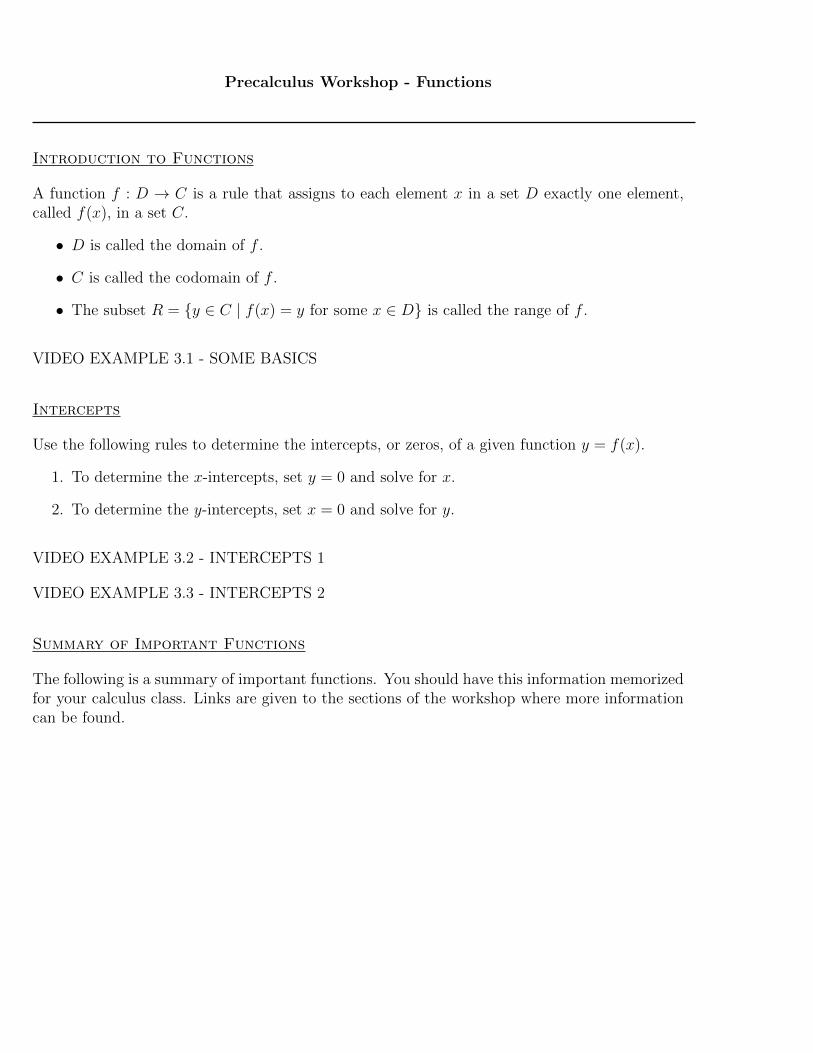
1. Basic Linear Function: f(x) = x (more on linear functions)

• Domain: (−∞,∞) = {x | x ∈ R}• Range: (−∞,∞) = {y | y ∈ R}

Figure 1: Graph of the basic linear function f(x) = x.

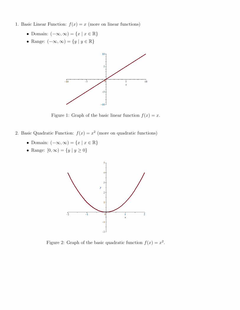
2. Basic Quadratic Function: f(x) = x2 (more on quadratic functions)

• Domain: (−∞,∞) = {x | x ∈ R}• Range: [0,∞) = {y | y ≥ 0}

Figure 2: Graph of the basic quadratic function f(x) = x2.

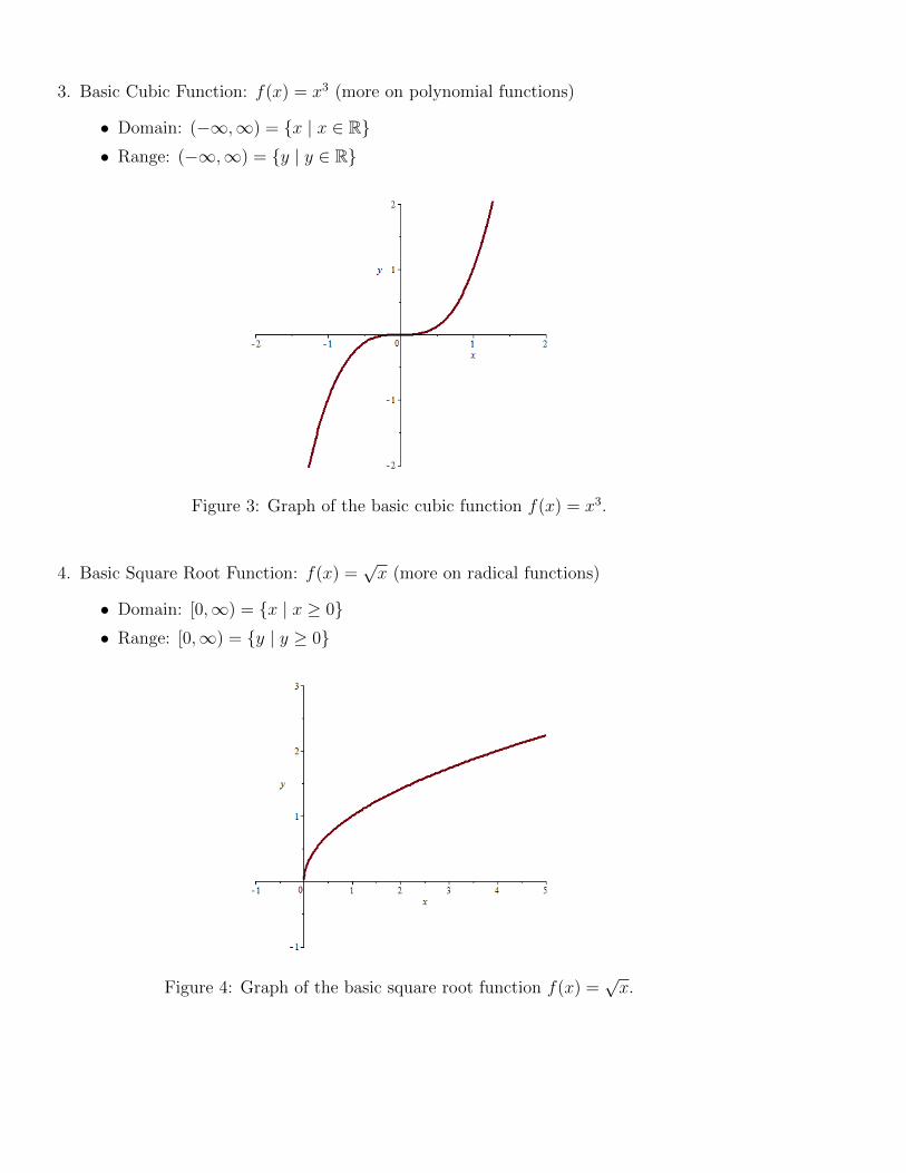
3. Basic Cubic Function: f(x) = x3 (more on polynomial functions)

• Domain: (−∞,∞) = {x | x ∈ R}• Range: (−∞,∞) = {y | y ∈ R}

Figure 3: Graph of the basic cubic function f(x) = x3.

4. Basic Square Root Function: f(x) =√x (more on radical functions)

• Domain: [0,∞) = {x | x ≥ 0}• Range: [0,∞) = {y | y ≥ 0}

Figure 4: Graph of the basic square root function f(x) =√x.

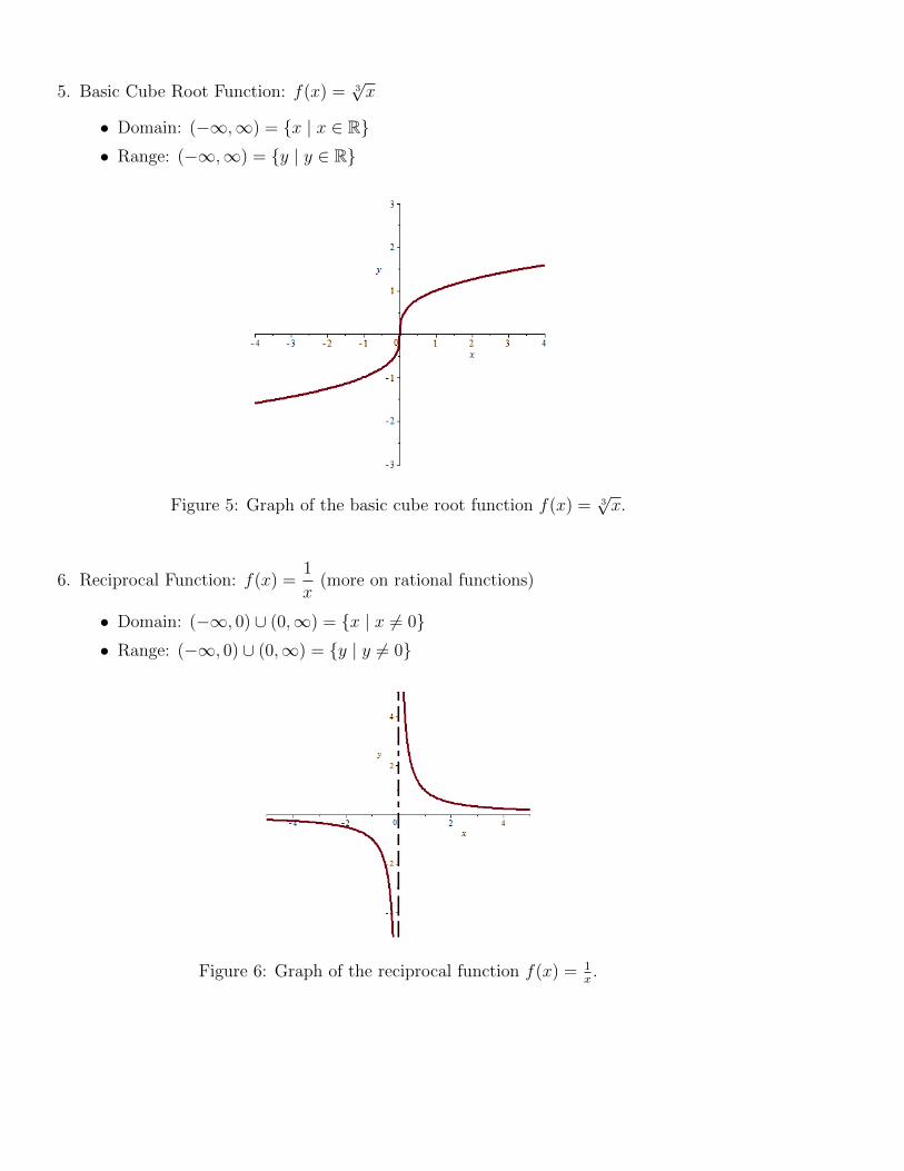
5. Basic Cube Root Function: f(x) = 3√x

• Domain: (−∞,∞) = {x | x ∈ R}• Range: (−∞,∞) = {y | y ∈ R}

Figure 5: Graph of the basic cube root function f(x) = 3√x.

6. Reciprocal Function: f(x) =1

x(more on rational functions)

• Domain: (−∞, 0) ∪ (0,∞) = {x | x 6= 0}• Range: (−∞, 0) ∪ (0,∞) = {y | y 6= 0}

Figure 6: Graph of the reciprocal function f(x) = 1x.

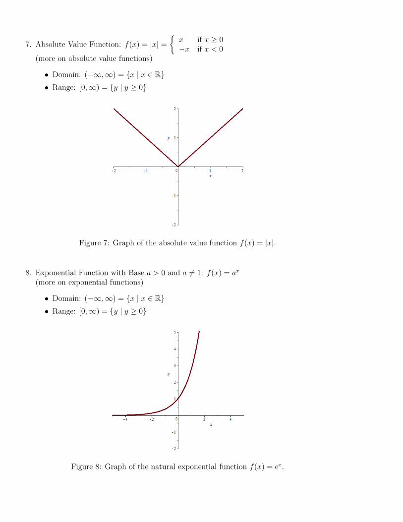
7. Absolute Value Function: f(x) = |x| ={x if x ≥ 0−x if x < 0

(more on absolute value functions)

• Domain: (−∞,∞) = {x | x ∈ R}• Range: [0,∞) = {y | y ≥ 0}

Figure 7: Graph of the absolute value function f(x) = |x|.

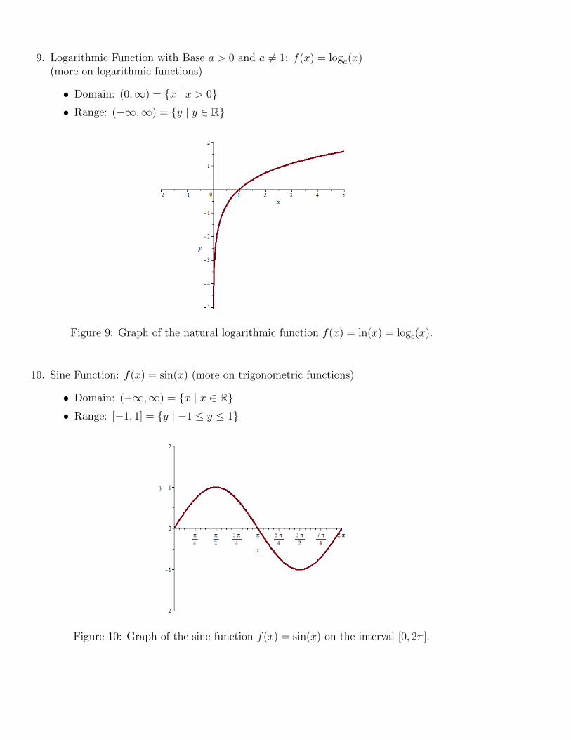
8. Exponential Function with Base a > 0 and a 6= 1: f(x) = ax

(more on exponential functions)

• Domain: (−∞,∞) = {x | x ∈ R}• Range: [0,∞) = {y | y ≥ 0}

Figure 8: Graph of the natural exponential function f(x) = ex.

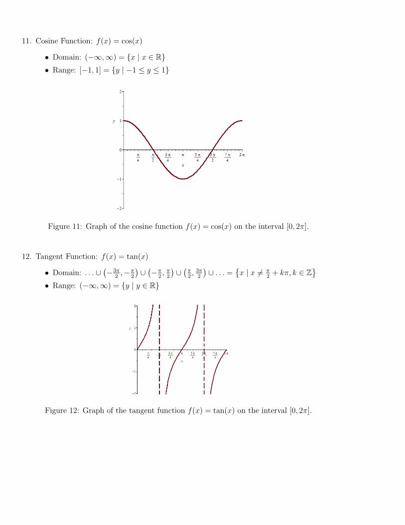
9. Logarithmic Function with Base a > 0 and a 6= 1: f(x) = loga(x)(more on logarithmic functions)

• Domain: (0,∞) = {x | x > 0}• Range: (−∞,∞) = {y | y ∈ R}

Figure 9: Graph of the natural logarithmic function f(x) = ln(x) = loge(x).

10. Sine Function: f(x) = sin(x) (more on trigonometric functions)

• Domain: (−∞,∞) = {x | x ∈ R}• Range: [−1, 1] = {y | −1 ≤ y ≤ 1}

Figure 10: Graph of the sine function f(x) = sin(x) on the interval [0, 2π].

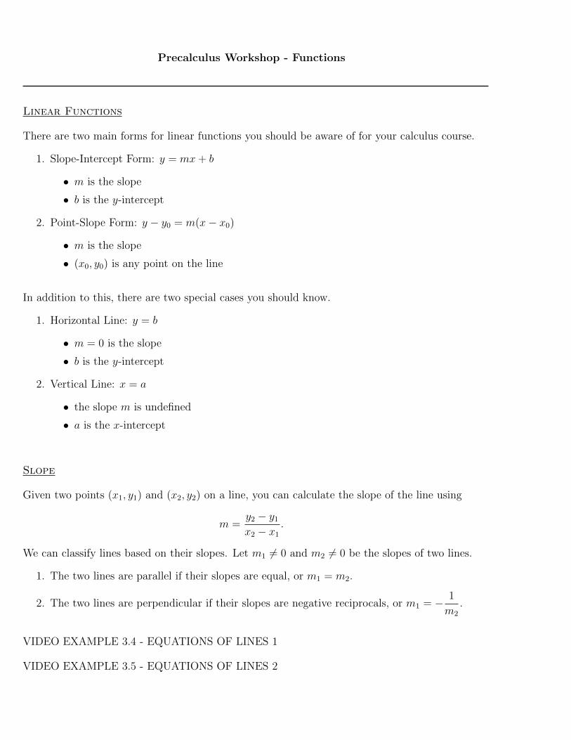
11. Cosine Function: f(x) = cos(x)

• Domain: (−∞,∞) = {x | x ∈ R}• Range: [−1, 1] = {y | −1 ≤ y ≤ 1}

Figure 11: Graph of the cosine function f(x) = cos(x) on the interval [0, 2π].

12. Tangent Function: f(x) = tan(x)

• Domain: . . . ∪(−3π

2,−π

2

)∪(−π

2, π2

)∪(π2, 3π

2

)∪ . . . =

{x | x 6= π

2+ kπ, k ∈ Z

}• Range: (−∞,∞) = {y | y ∈ R}

Figure 12: Graph of the tangent function f(x) = tan(x) on the interval [0, 2π].

Precalculus Workshop - Functions

Linear Functions

There are two main forms for linear functions you should be aware of for your calculus course.

1. Slope-Intercept Form: y = mx + b

• m is the slope

• b is the y-intercept

2. Point-Slope Form: y − y0 = m(x− x0)

• m is the slope

• (x0, y0) is any point on the line

In addition to this, there are two special cases you should know.

1. Horizontal Line: y = b

• m = 0 is the slope

• b is the y-intercept

2. Vertical Line: x = a

• the slope m is undefined

• a is the x-intercept

Slope

Given two points (x1, y1) and (x2, y2) on a line, you can calculate the slope of the line using

m =y2 − y1x2 − x1

.

We can classify lines based on their slopes. Let m1 6= 0 and m2 6= 0 be the slopes of two lines.

1. The two lines are parallel if their slopes are equal, or m1 = m2.

2. The two lines are perpendicular if their slopes are negative reciprocals, or m1 = − 1

m2

.

VIDEO EXAMPLE 3.4 - EQUATIONS OF LINES 1

VIDEO EXAMPLE 3.5 - EQUATIONS OF LINES 2

Precalculus Workshop - Functions

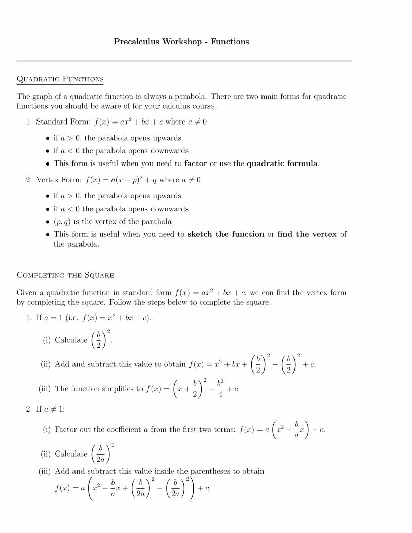
Quadratic Functions

The graph of a quadratic function is always a parabola. There are two main forms for quadraticfunctions you should be aware of for your calculus course.

1. Standard Form: f(x) = ax2 + bx + c where a 6= 0

• if a > 0, the parabola opens upwards

• if a < 0 the parabola opens downwards

• This form is useful when you need to factor or use the quadratic formula.

2. Vertex Form: f(x) = a(x− p)2 + q where a 6= 0

• if a > 0, the parabola opens upwards

• if a < 0 the parabola opens downwards

• (p, q) is the vertex of the parabola

• This form is useful when you need to sketch the function or find the vertex ofthe parabola.

Completing the Square

Given a quadratic function in standard form f(x) = ax2 + bx + c, we can find the vertex formby completing the square. Follow the steps below to complete the square.

1. If a = 1 (i.e. f(x) = x2 + bx + c):

(i) Calculate

(b

2

)2

.

(ii) Add and subtract this value to obtain f(x) = x2 + bx +

(b

2

)2

−(b

2

)2

+ c.

(iii) The function simplifies to f(x) =

(x +

b

2

)2

− b2

4+ c.

2. If a 6= 1:

(i) Factor out the coefficient a from the first two terms: f(x) = a

(x2 +

b

ax

)+ c.

(ii) Calculate

(b

2a

)2

.

(iii) Add and subtract this value inside the parentheses to obtain

f(x) = a

(x2 +

b

ax +

(b

2a

)2

−(

b

2a

)2)

+ c.

(iv) Remove −(

b

2a

)2

from the parentheses by multiplying by a:

f(x) = a

(x2 +

b

ax +

(b

2a

)2)− a ·

(b

2a

)2

+ c.

(v) The function simplifies to f(x) = a

(x +

b

2a

)2

− b2

4a+ c.

VIDEO EXAMPLE 3.6 - COMPLETING THE SQUARE

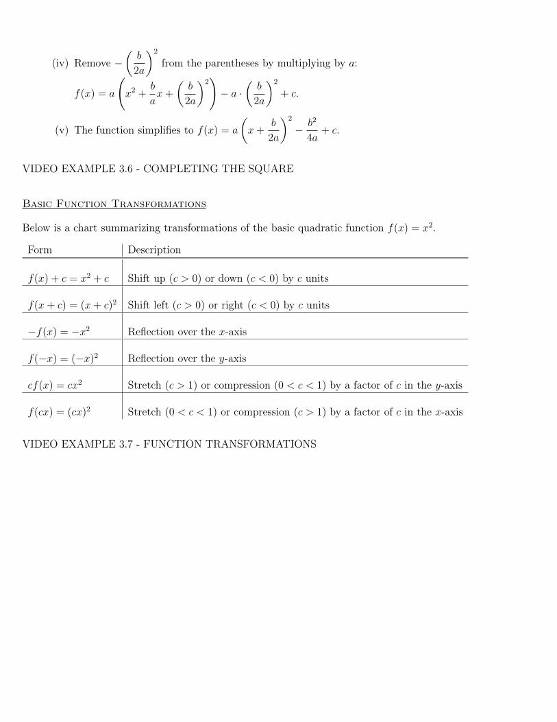
Basic Function Transformations

Below is a chart summarizing transformations of the basic quadratic function f(x) = x2.

Form Description

f(x) + c = x2 + c Shift up (c > 0) or down (c < 0) by c units

f(x + c) = (x + c)2 Shift left (c > 0) or right (c < 0) by c units

−f(x) = −x2 Reflection over the x-axis

f(−x) = (−x)2 Reflection over the y-axis

cf(x) = cx2 Stretch (c > 1) or compression (0 < c < 1) by a factor of c in the y-axis

f(cx) = (cx)2 Stretch (0 < c < 1) or compression (c > 1) by a factor of c in the x-axis

VIDEO EXAMPLE 3.7 - FUNCTION TRANSFORMATIONS

Precalculus Workshop - Functions

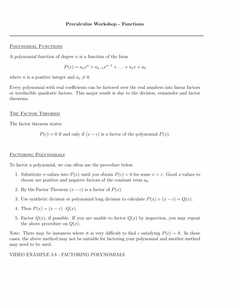
Polynomial Functions

A polynomial function of degree n is a function of the form

P (x) = anxn + an−1x

n−1 + . . . + a1x + a0

where n is a positive integer and an 6= 0.

Every polynomial with real coefficients can be factored over the real numbers into linear factorsor irreducible quadratic factors. This major result is due to the division, remainder and factortheorems.

The Factor Theorem

The factor theorem states:

P (c) = 0 if and only if (x− c) is a factor of the polynomial P (x).

Factoring Polynomials

To factor a polynomial, we can often use the procedure below.

1. Substitute x-values into P (x) until you obtain P (c) = 0 for some x = c. Good x-values tochoose are positive and negative factors of the constant term a0.

2. By the Factor Theorem (x− c) is a factor of P (x).

3. Use synthetic division or polynomial long division to calculate P (x)÷ (x− c) = Q(x).

4. Then P (x) = (x− c) ·Q(x).

5. Factor Q(x), if possible. If you are unable to factor Q(x) by inspection, you may repeatthe above procedure on Q(x).

Note: There may be instances where it is very difficult to find c satisfying P (c) = 0. In thesecases, the above method may not be suitable for factoring your polynomial and another methodmay need to be used.

VIDEO EXAMPLE 3.8 - FACTORING POLYNOMIALS

Precalculus Workshop - Functions

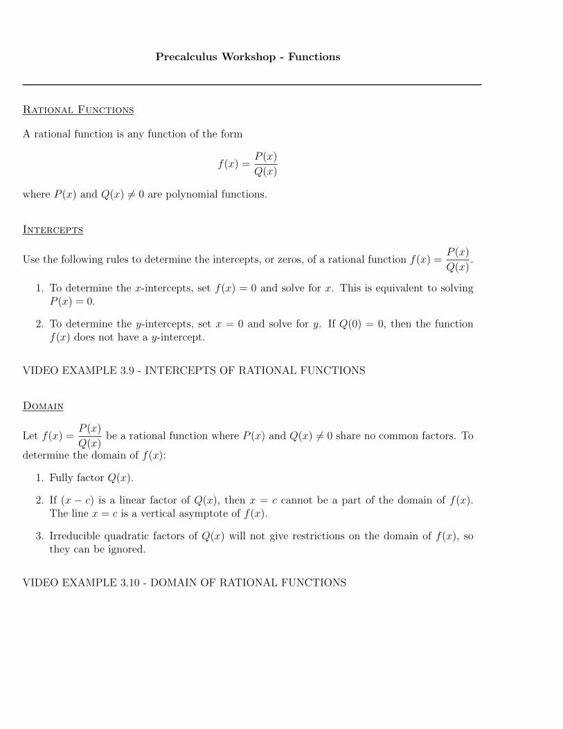
Rational Functions

A rational function is any function of the form

f(x) =P (x)

Q(x)

where P (x) and Q(x) 6= 0 are polynomial functions.

Intercepts

Use the following rules to determine the intercepts, or zeros, of a rational function f(x) =P (x)

Q(x).

1. To determine the x-intercepts, set f(x) = 0 and solve for x. This is equivalent to solvingP (x) = 0.

2. To determine the y-intercepts, set x = 0 and solve for y. If Q(0) = 0, then the functionf(x) does not have a y-intercept.

VIDEO EXAMPLE 3.9 - INTERCEPTS OF RATIONAL FUNCTIONS

Domain

Let f(x) =P (x)

Q(x)be a rational function where P (x) and Q(x) 6= 0 share no common factors. To

determine the domain of f(x):

1. Fully factor Q(x).

2. If (x − c) is a linear factor of Q(x), then x = c cannot be a part of the domain of f(x).The line x = c is a vertical asymptote of f(x).

3. Irreducible quadratic factors of Q(x) will not give restrictions on the domain of f(x), sothey can be ignored.

VIDEO EXAMPLE 3.10 - DOMAIN OF RATIONAL FUNCTIONS

Precalculus Workshop - Functions

Radical Functions

A radical function is any function of the form

f(x) = n√

P (x)

where P (x) is a polynomial function of degree 1 or higher. We will only consider the case whereP (x) is a polynomial of degree 1, that is, P (x) = mx + b, m 6= 0.

Intercepts

Use the following rules to determine the intercepts, or zeros, of a radical function f(x) = n√

P (x).

1. To determine the x-intercepts, set f(x) = 0 and solve for x. This is equivalent to solvingP (x) = 0.

2. To determine the y-intercepts, set x = 0 and solve for y. If P (0) < 0, then the functionf(x) does not have a y-intercept.

VIDEO EXAMPLE 3.11 - INTERCEPTS OF RADICAL FUNCTIONS

Domain

Let f(x) = n√

P (x) be a radical function where P (x) = mx + b, m 6= 0. To find the domain off(x) use the following rules:

1. If n is odd, f(x) has domain (−∞,∞) = {x | x ∈ R}.

2. If n is even, solve the inequality P (x) ≥ 0.

VIDEO EXAMPLE 3.12 - DOMAIN OF RADICAL FUNCTIONS

Precalculus Workshop - Functions

Piecewise Functions

A piecewise function is defined by using different formulas on different parts of its domain.

f(x) =

formula 1 interval 1formula 2 interval 2...formula n interval n

Evaluating Piecewise Functions

To evaluate a piecewise function at x = a, first look on the right hand side to determine whichinterval contains x = a. Then substitute x = a into the corresponding formula.

VIDEO EXAMPLE 3.13 - EVALUATING PIECEWISE FUNCTIONS

Precalculus Workshop - Functions

Function Composition

If f(x) and g(x) are functions, the composition of f(x) and g(x) is defined to be

(f ◦ g)(x) = f(g(x)).

NOTE: In general f ◦ g 6= g ◦ f , as can be seen in the next example.

VIDEO EXAMPLE 3.14 - FUNCTION COMPOSITION

Domain

The domain of (f ◦ g)(x) = f(g(x)) is the set of all x such that x is in the domain of g(x), andg(x) is in the domain of f(x). To determine the domain of (f ◦ g)(x), you can use the followingprocedure.

1. Determine any values of x in which g(x) is undefined.

2. Determine any values of x in which f(g(x)) is undefined.

3. The domain of (f ◦ g)(x) is the set of real numbers minus the union of the sets from steps1. and 2.

VIDEO EXAMPLE 3.15 - DOMAIN OF COMPOSITION 1

VIDEO EXAMPLE 3.16 - DOMAIN OF COMPOSITION 2

Precalculus Workshop - Functions

One-to-One Functions

A function f : R→ R is called one-to-one if f(x1) = f(x2) implies x1 = x2, where x1, x2 ∈ R.

To show a function is one-to-one:

1. Begin with f(x1) = f(x2).

2. Evaluate f at x1 and f at x2 and set these expressions equal to each other.

3. Use algebra to simplify to x1 = x2.

VIDEO EXAMPLE 3.17 - PROVING A FUNCTION IS ONE-TO-ONE

Inverse Functions

If f : D → R is a one-to-one function with domain D and range R, then the inverse functionf−1 : R→ D has domain R and range D and is defined by

f−1(y) = x⇔ f(x) = y.

for all y ∈ R.

NOTE: f−1(x) 6= 1

f(x). We use [f(x)]−1 =

1

f(x)to denote the reciprocal of f(x).

If f(x) and f−1(x) are inverse functions, they satisfy the inverse function properties:

1. (f ◦ f−1)(x) = f(f−1(x)) = x for all x ∈ R.

2. (f−1 ◦ f)(x) = f−1(f(x)) = x for all x ∈ D.

Finding an Inverse Function

If f(x) is a one-to-one function, we can find its inverse by using the following procedure.

1. Write y = f(x).

2. Interchange x and y.

3. Solve the equation for y.

4. The resulting equation is y = f−1(x).

VIDEO EXAMPLE 3.18 - FINDING INVERSE FUNCTIONS