Precalculus Polynomial & Rational --- Part One V. J. Motto.
75
Precalculu s Polynomial & Rational --- Part One V. J. Motto
-
Upload
lauren-mckinney -
Category
Documents
-
view
224 -
download
2
Transcript of Precalculus Polynomial & Rational --- Part One V. J. Motto.
PrecalculusPolynomial & Rational --- Part One
V. J. Motto
Real Zeros of Polynomials
The Factor Theorem tells us that finding
the zeros of a polynomial is really the same
thing as factoring it into linear factors.
In this section, we study some algebraic
methods that help us find the real zeros
of a polynomial, and thereby factor the
polynomial.
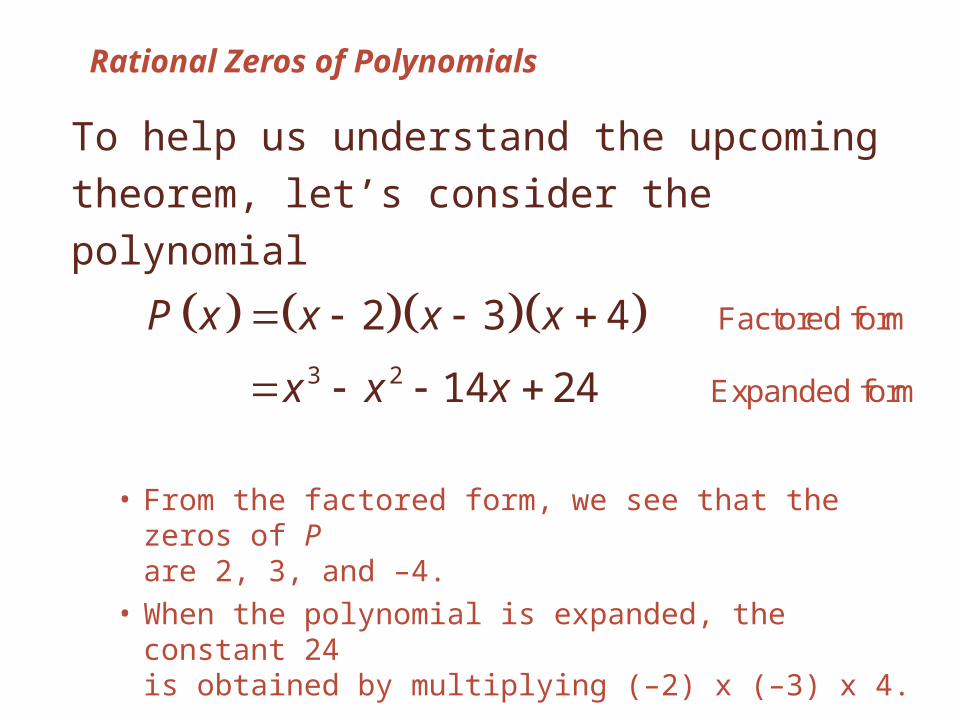
Rational Zeros of Polynomials
To help us understand the upcoming theorem,
let’s consider the polynomial
• From the factored form, we see that the zeros of P are 2, 3, and –4.
• When the polynomial is expanded, the constant 24 is obtained by multiplying (–2) x (–3) x 4.
3 2
Factored form
Expanded form
2 3 4
14 24
P x x x x
x x x

Rational Zeros of Polynomials
This means that the zeros of
the polynomial are all factors of
the constant term.
• The following generalizes this observation.

Rational Zeros Theorem
If the polynomial
has integer coefficients, then every rational
zero of P is of the form
where: • p is a factor of the constant coefficient a0.
• q is a factor of the leading coefficient an.
11 1 0
n nn nP x a x a x a x a
p
q

Rational Zeros Theorem—Proof
If p/q is a rational zero, in lowest terms,
of the polynomial P, we have:
1
1 1 0
1 11 1 0
1 2 11 1 0
0
0
n n
n n
n n n nn n
n n n nn n
p p pa a a a
q q q
a p a p q a pq a q
p a p a p q a q a q

Rational Zeros Theorem—Proof
Now, p is a factor of the left side, so it must be
a factor of the right as well.
As p/q is in lowest terms, p and q have no
factor in common; so, p must be a factor of a0.
• A similar proof shows that q is a factor of an.

Rational Zeros Theorem
From the theorem, we see that:
• If the leading coefficient is 1 or –1, the rational zeros must be factors of the constant term.

E.g. 1—Finding Rational Zeros (Leading Coefficient 1)
Find the rational zeros of
P(x) = x3 – 3x + 2
• Since the leading coefficient is 1, any rational zero must be a divisor of the constant term 2.
• So, the possible rational zeros are ±1 and ±2.
• We test each of these possibilities.

E.g. 1—Finding Rational Zeros (Leading Coefficient 1)
• The rational zeros of P are 1 and –2.
3
3
3
3
1 1 3 1 2 0
1 1 3 1 2 4
2 2 3 2 2 4
2 2 3 2 2 0
P
P
P
P

E.g. 2—Using the Theorem to Factor a Polynomial
Factor the polynomial
P(x) = 2x3 + x2 – 13x + 6
• By the theorem, the rational zeros of P are of the form
• The constant term is 6 and the leading coefficient is 2.• Thus,
Factor of constant termPossible rational zero of
Factor of leading coefficientP
Factor of 6Possible rational zero of
Factor of 2P

E.g. 2—Using the Theorem to Factor a Polynomial
The factors of 6 are: ±1, ±2, ±3, ±6
The factors of 2 are: ±1, ±2
• Thus, the possible rational zeros of P are:
1 2 3 6 1 2 3 6, , , , , , ,
1 1 1 1 2 2 2 2
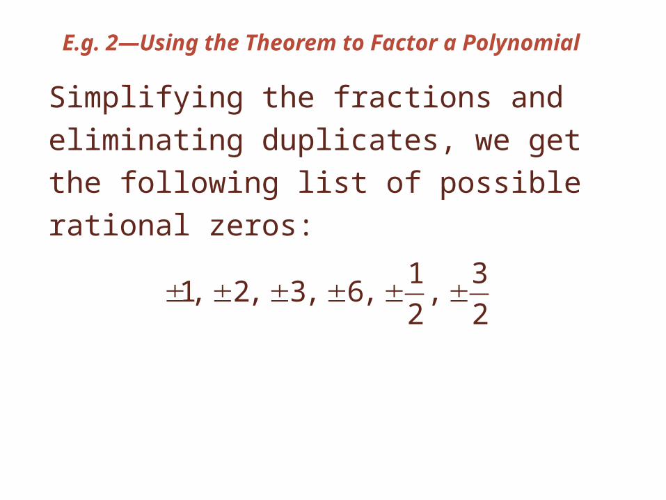
E.g. 2—Using the Theorem to Factor a Polynomial
Simplifying the fractions and eliminating
duplicates, we get the following list of
possible rational zeros:
1 31, 2, 3, 6, ,
2 2
E.g. 2—Using the Theorem to Factor a Polynomial
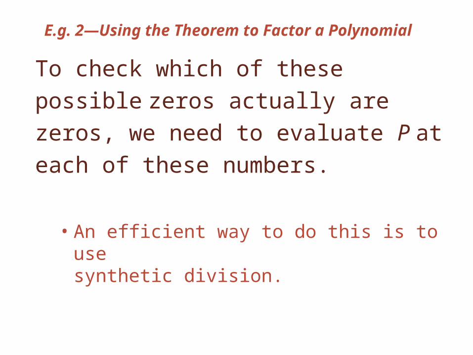
To check which of these possible zeros
actually are zeros, we need to evaluate P
at each of these numbers.
• An efficient way to do this is to use synthetic division.

E.g. 2—Using the Theorem to Factor a Polynomial
Test if 1 is a zero:
• Remainder is not 0.
• So, 1 is not a zero.
1 2 1 13 6
2 3 10
2 3 10 4

E.g. 2—Using the Theorem to Factor a Polynomial
Test if 2 is a zero:
• Remainder is 0.
• So, 2 is a zero.
2 2 1 13 6
4 10 6
2 5 3 0

E.g. 2—Using the Theorem to Factor a Polynomial
From the last synthetic division, we see that
2 is a zero of P and that P factors as:
3 2
2
2 13 6
2 2 5 3
2 2 1 3
P x x x x
x x x
x x x
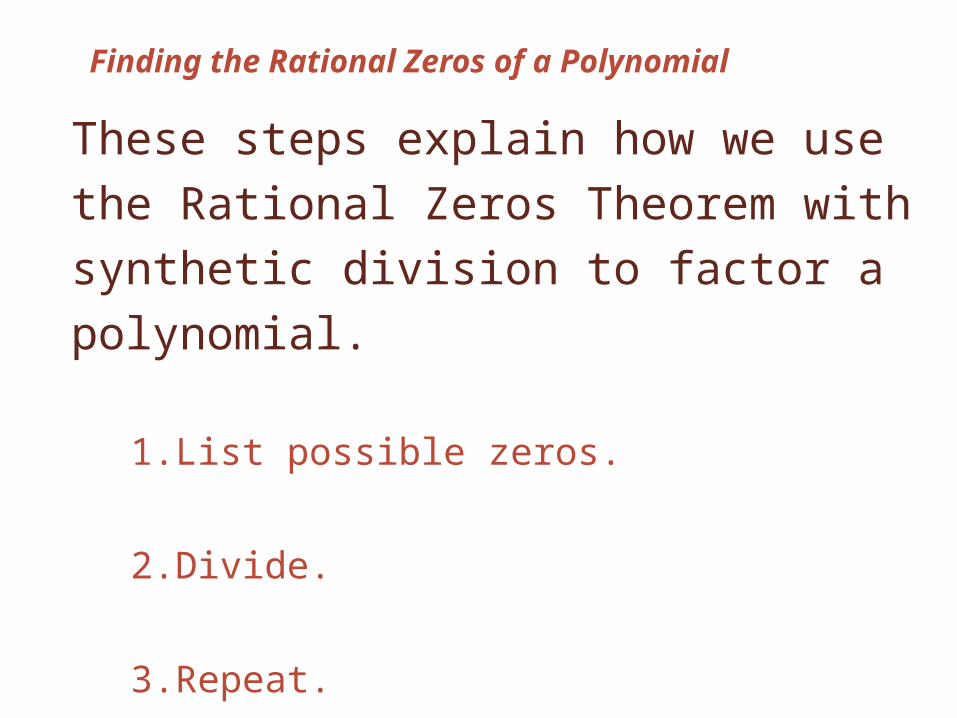
Finding the Rational Zeros of a Polynomial
These steps explain how we use the
Rational Zeros Theorem with synthetic
division to factor a polynomial.
1. List possible zeros.
2. Divide.
3. Repeat.

Step 1 to Finding the Rational Zeros of a Polynomial
List possible zeros.
• List all possible rational zeros using the Rational Zeros Theorem.

Step 2 to Finding the Rational Zeros of a Polynomial
Divide.
• Use synthetic division to evaluate the polynomial at each of the candidates for rational zeros that you found in Step 1.
• When the remainder is 0, note the quotient you have obtained.

Step 3 to Finding the Rational Zeros of a Polynomial
Repeat.
• Repeat Steps 1 and 2 for the quotient.
• Stop when you reach a quotient that is quadratic or factors easily.
• Use the quadratic formula or factor to find the remaining zeros.

E.g. 3—Using the Theorem and the Quadratic Formula
Let P(x) = x4 – 5x3 – 5x2 + 23x + 10.
(a) Find the zeros of P.
(b) Sketch the graph of P.

E.g. 3—Theorem & Quad. Formula
The leading coefficient of P is 1.
• So, all the rational zeros are integers.
• They are divisors of the constant term 10.
• Thus, the possible candidates are:
±1, ±2, ±5, ±10
Example (a)

E.g. 3—Theorem & Quad. Formula
Using synthetic division, we find that 1 and 2
are not zeros.
1 1 5 5 23 10
1 4 9 14
1 4 9 14 24
Example (a)
2 1 5 5 23 10
2 6 22 2
1 3 11 1 12

E.g. 3—Theorem & Quad. Formula
5 1 5 5 23 10
5 0 25 10
1 0 5 2 0
Example (a)
However, 5 is a zero.

E.g. 3—Theorem & Quad. Formula
Also, P factors as:
4 3 2
3
5 5 23 10
5 5 2
x x x x
x x x
Example (a)

E.g. 3—Theorem & Quad. Formula
We now try to factor the quotient
x3 – 5x – 2
• Its possible zeros are the divisors of –2, namely, ±1, ±2
• We already know that 1 and 2 are not zeros of the original polynomial P.
• So, we don’t need to try them again.
Example (a)

E.g. 3—Theorem & Quad. Formula
Checking the remaining candidates –1
and –2, we see that –2 is a zero.
Example (a)
2 1 0 5 2
2 4 2
1 2 1 0
E.g. 3—Theorem & Quad. Formula
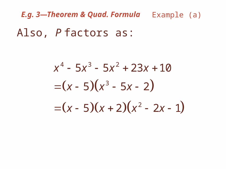
Also, P factors as:
4 3 2
3
2
5 5 23 10
5 5 2
5 2 2 1
x x x x
x x x
x x x x
Example (a)

E.g. 3—Theorem & Quad. Formula
Now, we use the quadratic formula to
obtain the two remaining zeros of P:
• The zeros of P are: 5, –2 , ,
22 2 4 1 1
1 22
x
1 2 1 2
Example (a)

E.g. 3—Theorem & Quad. Formula
Now that we know the zeros of P, we can
use the methods of Section 3-1 to sketch
the graph.
• If we want to use a graphing calculator instead, knowing the zeros allows us to choose an appropriate viewing rectangle.
• It should be wide enough to contain all the x-intercepts of P.
Example (b)

E.g. 3—Theorem & Quad. Formula
Numerical approximations to the zeros
of P are:
5, –2, 2.4, –0.4
Example (b)

E.g. 3—Theorem & Quad. Formula
So, in this case, we choose the rectangle
[–3, 6] by [–50, 50] and draw the graph.
Example (b)

Descartes’ Rule of Signs and
Upper and Lower Bounds for Roots

Descartes’ Rule of Signs
In some cases, the following rule is helpful
in eliminating candidates from lengthy lists
of possible rational roots.
• It was discovered by the French philosopher and mathematician René Descartes around 1637.

Variation in Sign
To describe this rule, we need
the concept of variation in sign.
• Suppose P(x) is a polynomial with real coefficients, written with descending powers of x (and omitting powers with coefficient 0).
• A variation in sign occurs whenever adjacent coefficients have opposite signs.

Variation in Sign
For example,
P(x) = 5x7 – 3x5 – x4 + 2x2 + x – 3
has three variations in sign.

Descartes’ Rule of Signs
Let P be a polynomial with real coefficients.
1. The number of positive real zeros of P(x) is either equal to the number of variations in sign in P(x) or is less than that by an even whole number.
2. The number of negative real zeros of P(x) is either equal to the number of variations in sign in P(-x) or is less than that by an even whole number.

E.g. 4—Using Descartes’ Rule
Use Descartes’ Rule of Signs to determine
the possible number of positive and negative
real zeros of the polynomial
P(x) = 3x6 + 4x5 + 3x3 – x – 3
• The polynomial has one variation in sign.
• So, it has one positive zero.

E.g. 4—Using Descartes’ Rule
Now,
P(–x) = 3(–x)6 + 4(–x)5 +3(–x)3 – (–x) – 3
= 3x6 – 4x5 – 3x3 + x – 3
• Thus, P(–x) has three variations in sign.
• So, P(x) has either three or one negative zero(s), making a total of either two or four real zeros.
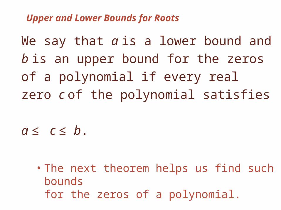
Upper and Lower Bounds for Roots
We say that a is a lower bound and b is an
upper bound for the zeros of a polynomial if
every real zero c of the polynomial satisfies
a ≤ c ≤ b.
• The next theorem helps us find such bounds for the zeros of a polynomial.

The Upper and Lower Bounds Theorem
Let P be a polynomial with real coefficients.
• If we divide P(x) by x – b (with b > 0) using synthetic division, and if the row that contains the quotient and remainder has no negative entry, then b is an upper bound for the real zeros of P.
• If we divide P(x) by x – a (with a < 0) using synthetic division, and if the row that contains the quotient and remainder has entries that are alternately nonpositive and nonnegative, then a is a lower bound for the real zeros of P.

Upper and Lower Bounds Theorem
A proof of this theorem is suggested in
Exercise 91.
The phrase “alternately nonpositive and
nonnegative” simply means that:
• The signs of the numbers alternate, with 0 considered to be positive or negative as required.

E.g. 5—Upper & Lower Bounds for Zeros of Polynomial
Show that all the real zeros of the polynomial
P(x) = x4 – 3x2 + 2x – 5
lie between –3 and 2.
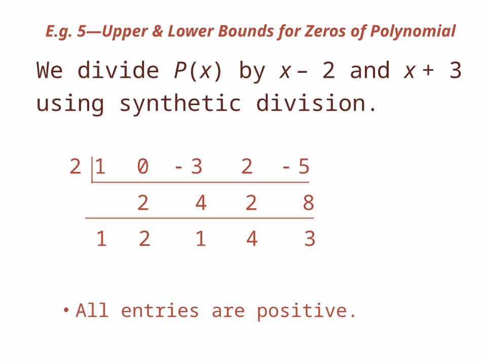
E.g. 5—Upper & Lower Bounds for Zeros of Polynomial
We divide P(x) by x – 2 and x + 3 using
synthetic division.
• All entries are positive.
2 1 0 3 2 5
2 4 2 8
1 2 1 4 3

E.g. 5—Upper & Lower Bounds for Zeros of Polynomial
• Entries alternate in sign.
3 1 0 3 2 5
3 9 18 48
1 3 6 16 43

E.g. 5—Upper & Lower Bounds for Zeros of Polynomial
By the Upper and Lower Bounds Theorem,
–3 is a lower bound and 2 is an upper
bound for the zeros.
• Neither –3 nor 2 is a zero (the remainders are not 0 in the division table).
• So, all the real zeros lie between these numbers.

E.g. 6—Factoring a Fifth-Degree Polynomial
Factor completely the polynomial
P(x) = 2x5 + 5x4 – 8x3 – 14x2 + 6x + 9
• The possible rational zeros of P are:
±½ , ±1, ±3/2, ±3, ±9/2, ±9
• We check the positive candidates first, beginning with the smallest.

E.g. 6—Factoring a Fifth-Degree Polynomial
• ½ is not a zero.
12
5 33 92 4 8
33 9 632 4 8
2 5 8 14 6 9
1 3
2 6 5

E.g. 6—Factoring a Fifth-Degree Polynomial
• P(1) = 0.
1 2 5 8 14 6 9
2 7 1 15 9
2 7 1 15 9 0

E.g. 6—Factoring a Fifth-Degree Polynomial
Thus, 1 is a zero,
and
P(x) = (x – 1)(2x4 + 7x3 – x2 – 15x – 9)

E.g. 6—Factoring a Fifth-Degree Polynomial
We continue by factoring the
quotient.
• We still have the same list of possible zeros, except that ½ has been eliminated.

E.g. 6—Factoring a Fifth-Degree Polynomial
• 1 is not a zero.
1 2 7 1 15 9
2 9 8 7
2 9 8 7 16

E.g. 6—Factoring a Fifth-Degree Polynomial
• P(3/2) = 0, (remainder is 0) all entries nonnegative.
32 2 7 1 15 9
3 15 21 9
2 10 14 6 0

E.g. 6—Factoring a Fifth-Degree Polynomial
We see that 3/2 is both a zero and
an upper bound for the zeros of P(x).
• So, we don’t need to check any further for positive zeros.
• All the remaining candidates are greater than 3/2.

E.g. 6—Factoring a Fifth-Degree Polynomial
P(x) = (x – 1)(x – 3/2)(2x3 + 10x2 + 14x + 6)
= (x – 1)(2x – 3)(x3 + 5x2 + 7x + 3)
• By Descartes’ Rule, x3 + 5x2 + 7x + 3 has no positive zero.
• So, its only possible rational zeros are –1 and –3.

E.g. 6—Factoring a Fifth-Degree Polynomial
• P(–1) = 0.
1 1 5 7 3
1 4 3
1 4 3 0

E.g. 6—Factoring a Fifth-Degree Polynomial
Therefore,
P(x) = (x – 1)(2x – 3)(x + 1)(x2 + 4x + 3)
= (x – 1)(2x – 3)(x + 1)2(x + 3)
• This means that the zeros of P are:
1, 3/2, –1, –3

E.g. 6—Factoring a Fifth-Degree Polynomial
The graph of the polynomial is shown
here.

Using Algebra and Graphing Devices
to Solve Polynomial Equations

Using Algebra and Graphing Devices
In Section 1-9, we used graphing devices to
solve equations graphically.
We can now use the algebraic techniques
we’ve learned to select an appropriate
viewing rectangle when solving a polynomial
equation graphically.

E.g. 7—Solving a Fourth-Degree Equation Graphically
Find all real solutions of the following
equation, correct to the nearest tenth.
3x4 + 4x3 – 7x2 – 2x – 3 = 0
• To solve the equation graphically, we graph:
P(x) = 3x4 + 4x3 – 7x2 – 2x – 3

E.g. 7—Solving a Fourth-Degree Equation Graphically
First, we use the Upper and Lower Bounds
Theorem to find two numbers between
which all the solutions must lie.
• This allows us to choose a viewing rectangle that is certain to contain all the x-intercepts of P.
• We use synthetic division and proceed bytrial and error.

E.g. 7—Solving a Fourth-Degree Equation Graphically
To find an upper bound, we try the whole
numbers, 1, 2, 3, . . . as potential candidates.
• We see that 2 is an upper bound for the roots.
• All entries are positive.
2 3 4 7 2 3
6 20 26 48
3 10 13 24 45

E.g. 7—Solving a Fourth-Degree Equation Graphically
Now, we look for a lower bound, trying
–1, –2, and –3 as potential candidates.
• We see that –3 is a lower bound for the roots.
• Entries alternate in sign.
3 3 4 7 2 3
9 15 24 78
3 5 8 26 75

E.g. 7—Solving a Fourth-Degree Equation Graphically
Thus, all the roots lie between –3
and 2.
• So, the viewing rectangle [–3, 2] by [–20,20] contains all the x-intercepts of P.
E.g. 7—Solving a Fourth-Degree Equation Graphically
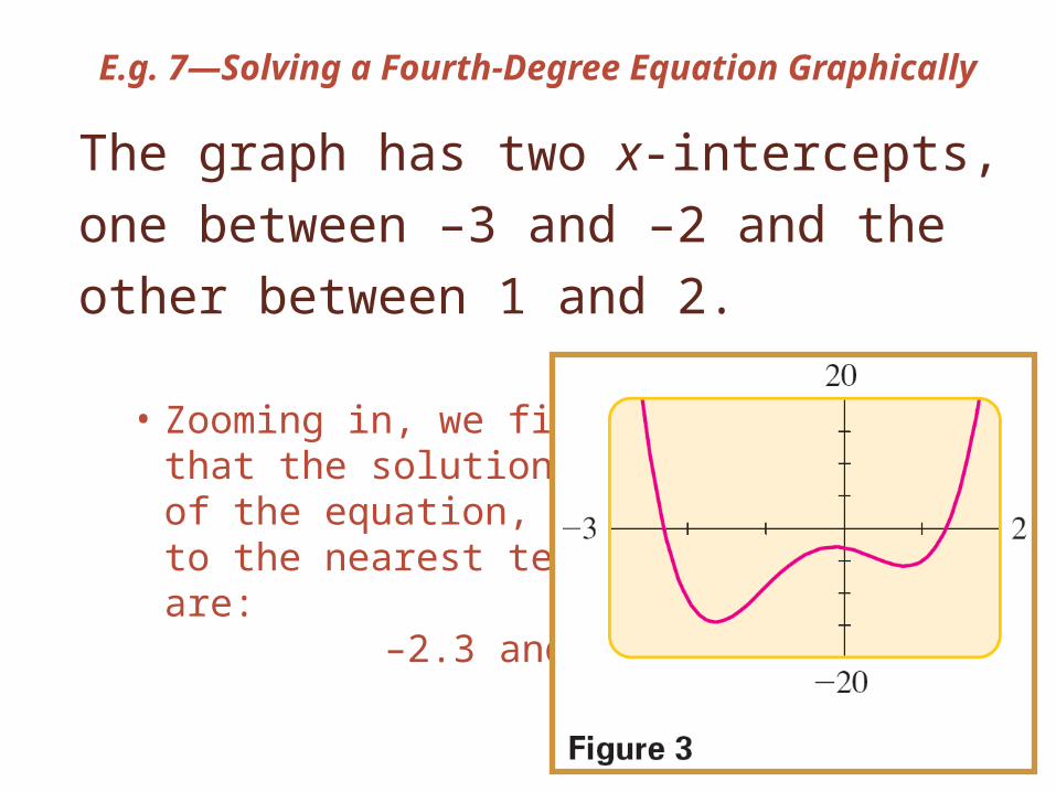
The graph has two x-intercepts, one
between –3 and –2 and the other between
1 and 2.
• Zooming in, we find that the solutions of the equation, to the nearest tenth, are:
–2.3 and 1.3

E.g. 8—Determining the Size of a Fuel Tank
A fuel tank consists of a cylindrical center
section 4 ft long and two hemispherical end
sections.• If the tank has a volume of 100 ft3,
what is the radius r, correct to the nearest hundredth of a foot?

E.g. 8—Determining the Size of a Fuel Tank
Using the volume formula (volume of
a cylinder: V = πr2h), we see that the volume
of the cylindrical section of the tank is:
π · r2 · 4

E.g. 8—Determining the Size of a Fuel Tank
The two hemispherical parts together form
a complete sphere whose volume (volume
of a sphere: V = 4/3πr3) is:
4/3πr3

E.g. 8—Determining the Size of a Fuel Tank
As the total volume of the tank is 100 ft3,
we get the equation:
4/3πr3 + 4πr2 = 100
E.g. 8—Determining the Size of a Fuel Tank
A negative solution for r would be
meaningless in this physical situation.
Also, by substitution, we can verify that r = 3
leads to a tank that is over 226 ft3 in volume—
much larger than the required 100 ft3.
• Thus, we know the correct radius lies somewhere between 0 and 3 ft.

E.g. 8—Determining the Size of a Fuel Tank
So, we use a viewing rectangle of [0, 3] by
[50, 150] to graph the function
y = 4/3πx3 + 4πx2
• We want the value of the function to be 100.
• Hence, we also graph the horizontal line y = 100 in the same viewing rectangle.

E.g. 8—Determining the Size of a Fuel Tank
The correct radius will be the x-coordinate
of the point of intersection of the curve and
the line.• Using the cursor and
zooming in, we see that, at the point of intersection, x ≈ 2.15, correct to two decimal places.
• So, the tank has a radius of about 2.15 ft.

Determining the Size of a Fuel Tank
Note that we also could have solved
the equation in Example 8 as follows.
1. We write it as: 4/3πr3 + 4πr2 – 100 = 0
2. We find the x-intercept of the function
y = 4/3πx3 + 4πx2 – 100