Pre Calculus I
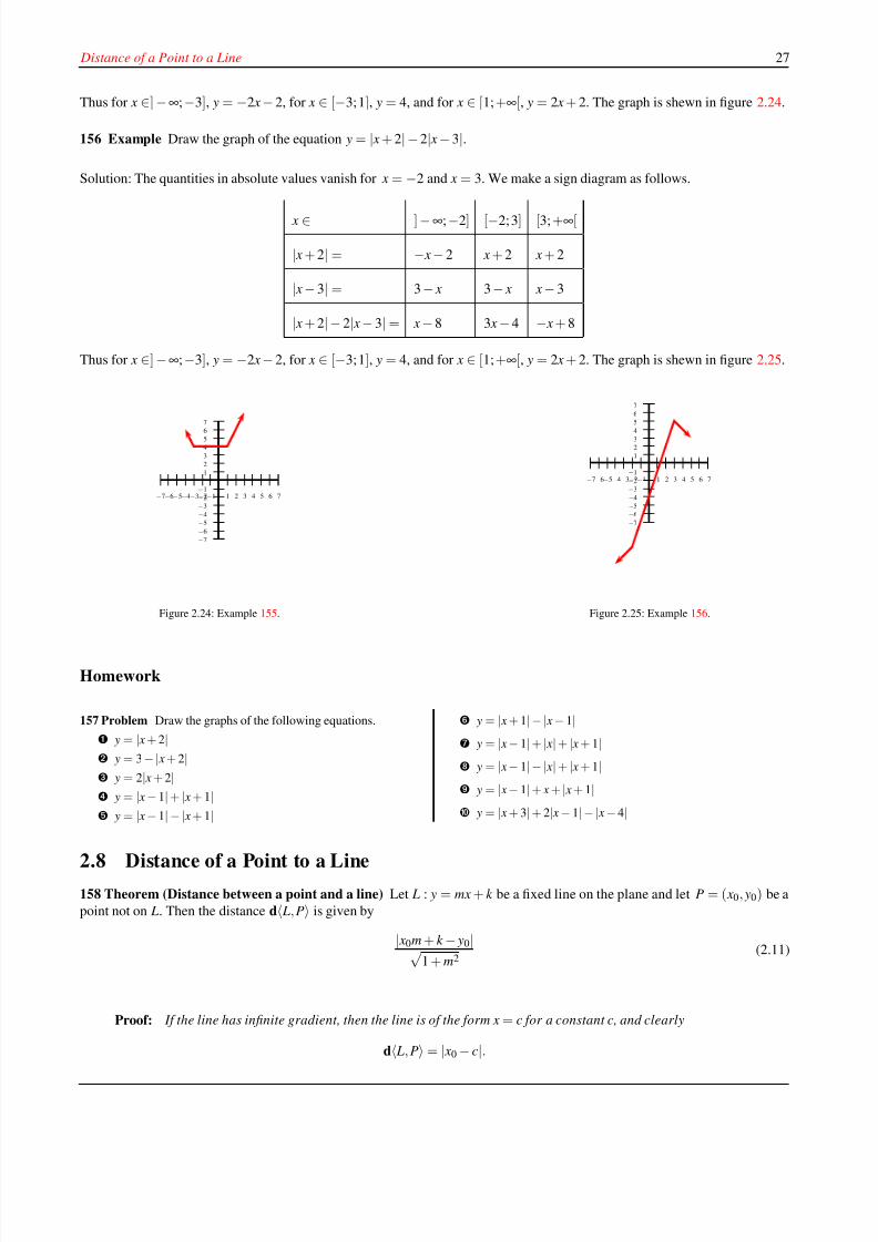
125
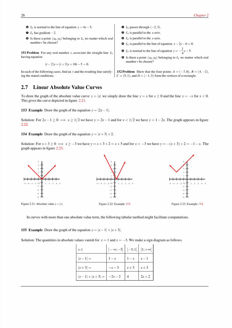
l c u l u s r e c a l c u l u s I P r e c a l c u s I P r e u s I P r e c P r e c a l c u l c u l u s I P r r e c a l c u e c a l c u l u s I P r e c r e c a l c u l P r e c a l c u l P r e c a l c u l u I P r e c a l c u P r e c a e c a l c u l u s I P r e c a l u s I l u a l c u l u s I r e c a l c u l u s r c P r e c a l c u l s I P r e c a u s I P r e c r l c u l u s I P r e c a l c u l u s I l u s P r e c a l c u l u s I P r e u s I P r e c a P r e c a u l u s I P e c a l c u P r e c a l u l u s I l c u l u s I P r e c a u l u s I l u s I P r e s I P r e c a l c u I P c u l u s I P r e c a P r e c a l c u l u e c a l c u l u s I P r e c a l c u l u P r e c a l c u a l c u l u s P r e c a a l c u l u s I P r e c l c u l u P r e c a r e c a l c u r e c a l c u l u s I r P r e c a l c u l u s l c u l u s I P c u l u u l u s I e c a l c u l u s I P r e u s I P r r r e c a l c u P r e c a l c u l u s I P I P r e c a r e c a l c u c a l c u l u s I l u s I P r e e c a l c u l u s I P r e c a l c u l u a l c u l u s I I P r e c a l r e c a l c u l u I P r e I P r e c a l c r l u s I P r e P r e c a l c u l u l c u l u s I u l u s I P r e c a l c u l u s I u l u s l c u l u s I l u s I c a l c u l u u s I P r e c a l c u l u u s I P c a l c u l u l c u l u s l c u l u s I P r e c a r e c a l c u l u s u s I P r e c a l c P r e c a l c u s I P r e c a l c u u l u s I P r r e c a l c u l u s l c u l u u l u s I I P r e c a l c e c a l c u l u s l u s I r l u s I P r e c P r e c a l c u I P r e c a l c u l u s I P s I P r e c a r e c a l c u l u s c u l u s I P r David A. Santos [email protected] August 26, 2005VERSION
-
Upload
jafet-lugo-gomez -
Category
Documents
-
view
241 -
download
1
Transcript of Pre Calculus I
8/8/2019 Pre Calculus I
http://slidepdf.com/reader/full/pre-calculus-i 1/125
l c u l u s
r e c a l c u l u s
I
P r e c
a l c u
sI
P r e
u sI
P r e c
P r e c
a l c u
l c u l u
sI
P r
r e c a l c u
e c a l c u l
u sI
P r e c
r e c a l c u l
P r e c
a l c u l
P r e c
a l c u l u
IP r e c
a l c u
P r e c
a
e c a l c u l u
sI
P r e c
a
l u s
I
l u
a l c u l u
sI
r e c a l c u l u s
rc
P
r e c a l c u l
sI
P r e c
a
u sI
P r e c
r
l c u l u s
IP r
e c a l c u l u
sI
l u s
P r e c
a l c u l u
sI
P r e
u sI
P r e c
a
P r e c a
u l u s
IP e
c a l c u
P r e c
a l
u l u s
I
l c
u l u s
IP r e c
a
u l u s
I
l u s
IP r e
sI
P r e c
a l c u
I
P
c u l u
sI
P r e c a
P r e c
a l c u l u
e c a l c u l u
sI
P r e c
a l c u l u
P r e c a l
c u
a l c u l u
s
P r e c
a
a l c u l u
s
IP r e c
l c u l u
P r e c
a
r e c a l c u
r e c a l c u l u s
I
r
P r e c a l c u l u s
l c u l u s
IP
c u l u
u l u s
I
e c a l c u l u s
IP r e
u sI
P r
r
r e c a l c u
P
r e c a l c u l u s
IP
IP r e c
a
r e c a l c u
c a l c u l u
sI
l u s
IP r e
e c a l c u l u
sI
P r e c
a l c u
l u
a l c u l u
sI
IP r e c a l
r e c a l c u l u
IP r e
IP r e c
a l c
r
l u s
IP r e
P r e c a l c u l u
l c u l u s
I
u l u s
IP r e c
a l c u l u
sI
u l u s
l c u l u
sI
l u s
I
c a l c u l u
u sI
P r
e c a l c u l u
u sI
P
c a l c u l u
l c u l u s
l c u l u s
IP r e c a
r e c a l c u l u s
u sI
P r e c
a l c
P r e c
a l c u
sI P
r e c
a l c u
u l u s
IP r
r e c a l c u l u s
l c u l u
u l u s
I
IP r e c
a l c
e c a l c u l u
s
l u s
I
r
l u sI
P r e c
P r e c
a l c u
IP r e c a l c u l u s
I P
sI
P r e c
a
r e c a l c u l u s
c u l u
sI
P r
David A. [email protected]
August 26, 2005VERSION
8/8/2019 Pre Calculus I
http://slidepdf.com/reader/full/pre-calculus-i 2/125
ii
Contents
Preface iii
To the Student iv
1 Numbers and Notation 1
1.1 The Real Line . . . . . . . . . . . . . . . . . 1Homework . . . . . . . . . . . . . . . . . . 5
1.2 Intervals . . . . . . . . . . . . . . . . . . . . 6
Homework . . . . . . . . . . . . . . . . . . 7
1.3 Sets on the Plane . . . . . . . . . . . . . . . 8
Homework . . . . . . . . . . . . . . . . . . 9
1.4 Neighbourhood of a point . . . . . . . . . . . 9
Answers . . . . . . . . . . . . . . . . . . . . . . . 10
2 Distance and Curves on the Plane 11
2.1 Distance on the Real Line . . . . . . . . . . . 11
Homework . . . . . . . . . . . . . . . . . . 13
2.2 Distance on the Real Plane . . . . . . . . . . 13
Homework . . . . . . . . . . . . . . . . . . 152.3 Circles . . . . . . . . . . . . . . . . . . . . . 16
Homework . . . . . . . . . . . . . . . . . . 17
2.4 Semicircles . . . . . . . . . . . . . . . . . . 18
Homework . . . . . . . . . . . . . . . . . . 20
2.5 Lines . . . . . . . . . . . . . . . . . . . . . 20
Homework . . . . . . . . . . . . . . . . . . 22
2.6 Parallel and Perpendicular Lines . . . . . . . 23
Homework . . . . . . . . . . . . . . . . . . 25
2.7 Linear Absolute Value Curves . . . . . . . . 26
Homework . . . . . . . . . . . . . . . . . . 27
2.8 Distance of a Point to a Line . . . . . . . . . 27
Homework . . . . . . . . . . . . . . . . . . 28
2.9 Parabolas . . . . . . . . . . . . . . . . . . . 28Homework . . . . . . . . . . . . . . . . . . 29
2.10 Hyperbolas . . . . . . . . . . . . . . . . . . 29
Answers . . . . . . . . . . . . . . . . . . . . . . . 31
3 Functions I: Assignment Rules 33
3.1 Basic Definitions . . . . . . . . . . . . . . . 33
Homework . . . . . . . . . . . . . . . . . . 37
3.2 Piecewise Functions . . . . . . . . . . . . . . 38
Homework . . . . . . . . . . . . . . . . . . 40
3.3 Translations . . . . . . . . . . . . . . . . . . 41
Homework . . . . . . . . . . . . . . . . . . 43
3.4 Distortions . . . . . . . . . . . . . . . . . . . 43
Homework . . . . . . . . . . . . . . . . . . 45
3.5 Reflexions . . . . . . . . . . . . . . . . . . . 45
Homework . . . . . . . . . . . . . . . . . . 46
3.6 Symmetry . . . . . . . . . . . . . . . . . . . 47
Homework . . . . . . . . . . . . . . . . . . 50
3.7 Behaviour of the Graphs of Functions . . . . 51
Homework . . . . . . . . . . . . . . . . . . 57Answers . . . . . . . . . . . . . . . . . . . . . . . 57
4 Functions II: Domains and Images 59
4.1 Natural Domain of an Assignment Rule . . . 59
Homework . . . . . . . . . . . . . . . . . . 61
4.2 Algebra of Functions . . . . . . . . . . . . . 61
Homework . . . . . . . . . . . . . . . . . . 67
4.3 Injections and Surjections . . . . . . . . . . . 68
Homework . . . . . . . . . . . . . . . . . . 71
4.4 Inversion . . . . . . . . . . . . . . . . . . . 71
Homework . . . . . . . . . . . . . . . . . . 74
Answers . . . . . . . . . . . . . . . . . . . . . . . 75
5 Polynomial Functions 77
5.1 Power Functions . . . . . . . . . . . . . . . 77
Homework . . . . . . . . . . . . . . . . . . 79
5.2 Affine Functions . . . . . . . . . . . . . . . 79
5.3 Quadratic Functions . . . . . . . . . . . . . . 80
Homework . . . . . . . . . . . . . . . . . . 84
5.4 Polynomials . . . . . . . . . . . . . . . . . . 84
5.4.1 Roots . . . . . . . . . . . . . . . . . 84
5.4.2 Ruffini’s Factor Theorem . . . . . . . 85
Homework . . . . . . . . . . . . . . . . . . 89
5.5 Graphs of Polynomials . . . . . . . . . . . . 89
Homework . . . . . . . . . . . . . . . . . . 91
Answers . . . . . . . . . . . . . . . . . . . . . . . 91
6 Rational Functions and Algebraic Functions 93
6.1 Inverse Power Functions . . . . . . . . . . . 93
6.2 Rational Functions . . . . . . . . . . . . . . 94
6.3 Algebraic Functions . . . . . . . . . . . . . . 96
Answers . . . . . . . . . . . . . . . . . . . . . . . 96
A Complex Numbers 97
A.1 Arithmetic of Complex Numbers . . . . . . . 97
A.2 Equations involving Complex Numbers . . . 99
Homework . . . . . . . . . . . . . . . . . . 100
B Sample Multiple-Choice Questions 101
8/8/2019 Pre Calculus I
http://slidepdf.com/reader/full/pre-calculus-i 3/125
iii
Preface
There are very few good Calculus books, written in English, available to the American reader. Only [ Har], [Kla], [Apo], [Olm],
and [Spi] come to mind.
The situation in Precalculus is even worse, perhaps because Precalculus is a peculiar American animal: it is a review course
of all that which should have been learned in High School but was not. A distinctive American slang is thus called to describe
the situation with available Precalculus textbooks: they stink!
I have decided to write these notes with the purpose to, at least locally, for my own students, I could ameliorate this situationand provide a semi-rigorous introduction to precalculus.
These notes are in constant state of revision. I would greatly appreciate comments, additions, exercises, figures, etc., in
order to help me enhance them. I would also like to begin translating them into Spanish. Any help would be appreciated.
David A. Santos
Legal Notice
This material may be distributed only subject to the terms and conditions set forth in the Open Publication License, version 1.0
or later (the latest version is presently available at http://www.opencontent.org/openpub/.
THIS WORK IS LICENSED AND PROVIDED “AS IS” WITHOUT WARRANTY OF ANY KIND, EXPRESS OR IM-
PLIED, INCLUDING, BUT NOT LIMITED TO, THE IMPLIED WARRANTIES OF MERCHANTABILITY AND FITNESS
FOR A PARTICULAR PURPOSE OR A WARRANTY OF NON-INFRINGEMENT.
THIS DOCUMENT MAY NOT BE SOLD FOR PROFIT OR INCORPORATED INTO COMMERCIAL DOCUMENTS
WITHOUT EXPRESS PERMISSION FROM THE AUTHOR(S). THIS DOCUMENT MAY BE FREELY DISTRIBUTED
PROVIDED THE NAME OF THE ORIGINAL AUTHOR(S) IS(ARE) KEPT AND ANY CHANGES TO IT NOTED.
8/8/2019 Pre Calculus I
http://slidepdf.com/reader/full/pre-calculus-i 4/125
To the Student
These notes are provided for your benefit as an attempt to organise the salient points of the course. They are a very terse account
of the main ideas of the course, and are to be used mostly to refer to central definitions and theorems. The number of examples
is minimal, and here you will not find exercises. The motivation or informal ideas of looking at a certain topic, the ideas linking
a topic with another, the worked-out examples, etc., are given in class. Hence these notes are not a substitute to lectures: you
must always attend to lectures. The order of the notes may not necessarily be the order followed in the class.
There is a certain algebraic fluency that is necessary for a course at this level. These algebraic prerequisites would be
difficult to codify here, as they vary depending on class response and the topic lectured. If at any stage you stumble in Algebra,
seek help! I am here to help you!
Tutoring can sometimes help, but bear in mind that whoever tutors you may not be familiar with my conventions. Again, I
am here to help! On the same vein, other books may help, but the approach presented here is at times unorthodox and finding
alternative sources might be difficult.
Here are more recommendations:
• Read a section before class discussion, in particular, read the definitions.
• Class provides the informal discussion, and you will profit from the comments of your classmates, as well as gainconfidence by providing your insights and interpretations of a topic. Don’t be absent!
• I encourage you to form study groups and to discuss the assignments. Discuss among yourselves and help each other but
don’t be parasites! Plagiarising your classmates’ answers will only lead you to disaster!
• Once the lecture of a particular topic has been given, take a fresh look at the notes of the lecture topic.
• Try to understand a single example well, rather than ill-digest multiple examples.
• Start working on the distributed homework ahead of time.
• Ask questions during the lecture. There are two main types of questions that you are likely to ask.
1. Questions of Correction: Is that a minus sign there? If you think that, for example, I have missed out a minus
sign or wrote P where it should have been Q,1 then by all means, ask. No one likes to carry an error till line XLV
because the audience failed to point out an error on line I. Don’t wait till the end of the class to point out an error.
Do it when there is still time to correct it!
2. Questions of Understanding: I don’t get it! Admitting that you do not understand something is an act requiring
utmost courage. But if you don’t, it is likely that many others in the audience also don’t. On the same vein, if you
feel you can explain a point to an inquiring classmate, I will allow you time in the lecture to do so. The best way to
ask a question is something like: “How did you get from the second step to the third step?” or “What does it mean
to complete the square?” Asseverations like “I don’t understand” do not help me answer your queries. If I consider
that you are asking the same questions too many times, it may be that you need extra help, in which case we will
settle what to do outside the lecture.
1My doctoral adviser used to say “I said A, I wrote B, I meant C and it should have been D!
iv

8/8/2019 Pre Calculus I
http://slidepdf.com/reader/full/pre-calculus-i 5/125
To the Student v
• Don’t fall behind! The sequence of topics is closely interrelated, with one topic leading to another.
• You will need square-grid paper, a ruler (preferably a T-square), some needle thread, and a compass.
• The use of calculators is allowed, especially in the occasional lengthy calculations. However, when graphing, you will
need to provide algebraic/analytic/geometric support of your arguments. The questions on assignments and exams will
be posed in such a way that it will be of no advantage to have a graphing calculator.
• Presentation is critical. Clearly outline your ideas. When writing solutions, outline major steps and write in completesentences. As a guide, you may try to emulate the style presented in the scant examples furnished in these notes.
8/8/2019 Pre Calculus I
http://slidepdf.com/reader/full/pre-calculus-i 6/125
vi
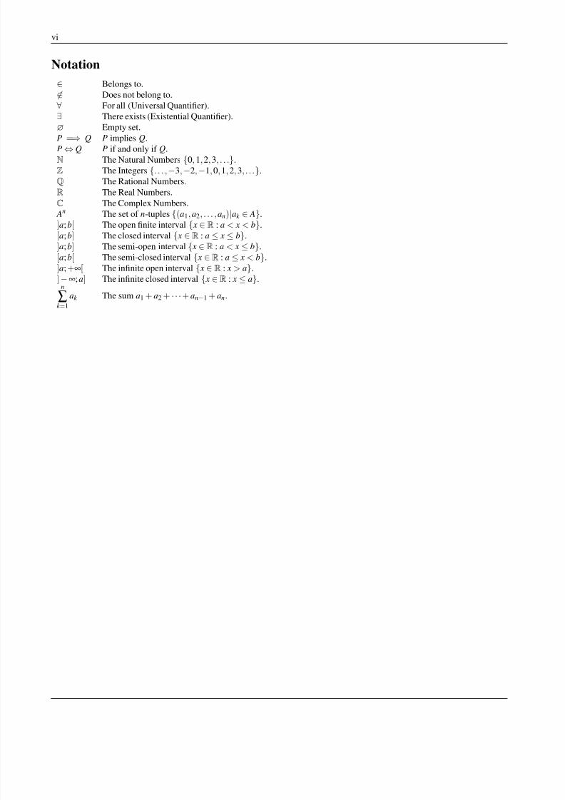
Notation
∈ Belongs to.∈ Does not belong to.∀ For all (Universal Quantifier).∃ There exists (Existential Quantifier).
∅ Empty set.
P =⇒ Q P implies Q.P ⇔ Q P if and only if Q.
N The Natural Numbers {0, 1, 2, 3, . . .}.
Z The Integers {. . . ,−3,−2,−1, 0, 1, 2, 3, . . .}.
Q The Rational Numbers.
R The Real Numbers.
C The Complex Numbers.
An The set of n-tuples {(a1, a2, . . . ,an)|ak ∈ A}.
]a; b[ The open finite interval { x ∈ R : a < x < b}.
[a; b] The closed interval { x ∈ R : a ≤ x ≤ b}.
]a; b] The semi-open interval { x ∈ R : a < x ≤ b}.
[a; b[ The semi-closed interval { x ∈ R : a ≤ x < b}.
]a; +∞[ The infinite open interval
{ x
∈R : x > a
}.
] −∞; a] The infinite closed interval { x ∈ R : x ≤ a}.n
∑k =1
ak The sum a1 + a2 + · · ·+ an−1 + an.
8/8/2019 Pre Calculus I
http://slidepdf.com/reader/full/pre-calculus-i 7/125
Chapter
1Numbers and Notation
This chapter introduces essential notation and terminology that will be used throughout these notes.
1.1 The Real Line
1 Definition We will mean by a set a collection of well defined members or elements. A subset is a sub-collection of a set. We
denote that B is a subset of A by the notation B ⊆ A or sometimes B ⊂ A.1
2 Definition Let A be a set. If a belongs to the set A, then we write a ∈ A, read “a is an element of A.” If a does not belong to
the set A, we write a ∈ A, read “a is not an element of A.” The set that has no elements, that is empty set , will be denoted by ∅.
We denote the set of natural numbers {0, 1, 2, . . .}2 by the symbol N. The natural numbers allow us to count things, and
they have the property that addition and multiplication is closed within them: that is, if we add or multiply two natural numbers,
we stay within the natural numbers. Observe that this is not true for subtraction and division, since, for example, neither 2 − 7
nor 2 ÷ 7 are natural numbers. We then say that the natural numbers enjoy closure within multiplication and addition.
3 Definition A prime number is a natural number p > 1 whose only divisors are 1 and p.
The first few primes are 2, 3, 5, 7, 11, 13, 17, 19, 23, 29, 31, . . .. We have the following fact, for which proof we refer the
reader to any number theory book.
4 Fact Any natural number greater than 1 can be factorised uniquely (except for the order of the factors) as a product of prime
numbers.
5 Example The prime factorisation of 2002 is 2 · 7 ·11 ·13.
That we have an inexhaustible source of primes has been known since Euclid, whose proof of the fact we now present.
6 Theorem (Euclid) There are infinitely many primes.
Proof: Let p1, p2, . . . pk be a list of primes. Construct the integer
n = p1 p2 · · · pk + 1.
This integer is greater than 1 and so by Fact 4 it must have a prime divisor p. Observe that p must be different from
any of p1, p2, . . . , pk since n leaves remainder 1 upon division by any of the pi. We have shown that no finite list of
primes exhausts the set of primes, i.e., that the set of primes is infinite.u
1There is no agreement relating the choice. Some use ⊂ to denote strict containment, but we will not need such subtleties in these notes.2We follow common European usage and include 0 among the natural numbers.
1
8/8/2019 Pre Calculus I
http://slidepdf.com/reader/full/pre-calculus-i 8/125
2 Chapter 1
By appending the opposite (additive inverse) of every member of N to N we obtain the set
Z= {. . . ,−3,−2,−1, 0, 1, 2, 3, . . .}3
of integers. The closure of multiplication and addition is retained by this extension and now we also have closure under
subtraction. Also, we have gained the notion of positivity. This last property allows us to divide the integers into the strictly
positive, the strictly negative or zero, and hence introduces an ordering in the rational numbers by defining a ≤ b if and only if
b − a is positive.Enter now in the picture the rational numbers, commonly called fractions, which we denote by the symbol Q.4 They are
the numbers of the forma
bwith a ∈ Z, b ∈ Z, b = 0, that is, the division of two integers, with the divisor distinct from zero.
Observe that every rational numbera
bis a solution to the equation (with x as the unknown) bx − a = 0. It can be shewn that
the rational numbers are precisely those numbers whose decimal representation either is finite (e.g., 0.123) or is periodic (e.g.,
0.123 = 0.123123123. . .). Notice that every integer is a rational number, sincea
1= a, for any a ∈ Z.
7 Example Write the infinitely repeating decimal 0.345 = 0.345454545. . . as the quotient of two natural numbers.
Solution: The trick is to obtain multiples of x = 0.345454545. . . so that they have the same infinite tail, and then subtract these
tails, cancelling them out.5 So observe that
10 x = 3.45454545. . . ;1000 x = 345.454545. . . =⇒ 1000 x − 10 x = 342 =⇒ x =342
990=
19
55.
Upon reaching Q we have formed a system of numbers having closure for the four arithmetical operations of addition,
subtraction, multiplication, or division. 6 These closure properties give us the following theorem.
8 Theorem Between any two different rational numbers there is another rational number.
Proof: If r , s are rational numbers with r < s, then their averager + s
2is also a rational number and satisfies
r <r + s
2< s. u
The last theorem implies that however close two rational numbers might be, we can always fit another rational number inbetween them. It is surprising, however, that we cannot “fill up the space between two rational numbers with just rational
numbers,” for we will demonstrate shortly that there are numbers which are not rational. Up until the Pythagoreans7, the ancient
Greeks thought that all numbers were the ratio of two integers. It was then discovered that the length of the hypothenuse of a
right triangle having both legs of unit length—which is√
2 in modern notation—could not be represented as the ratio of two
integers, that is, that√
2 is irrational8.
9 Theorem The number√
2 is irrational.
Proof: If √
2 were rational, then we would have, for some relatively prime positive integers,√
2 =a
b. This entails
a2 = 2b2. The sinistral side has an even number of prime factors (including repetitions), whereas the dextral side
has an odd number of prime factors. This is a contradiction to Fact 4 (unique factorisation), and hence√
2 is
irrational. u
Appending the irrational numbers to the rational numbers we obtain the real numbers R.
! The set of irrational numbers isR\Q.
3Z for the German word Z¨ ahlen, meaning number .4Q for quotients.5That this cancellation is meaningful depends on the concept of convergence, of which we may talk more later.6 “Reeling and Writhing, of course, to begin with, ”the Mock Turtle replied, “and the different branches of Arithmetic–Ambition, Distraction, Uglification,
and Derision.”7Pythagoras lived approximately from 582 to 500 BC. A legend says that the fact that
√2 was irrational was secret carefully guarded by the Pythagoreans.
One of them betrayed this secret, and hence was assassinated by being drowned from a ship.8An irrational number is thus one that cannot be written as the quotient of two integers
a
bwith b = 0.
8/8/2019 Pre Calculus I
http://slidepdf.com/reader/full/pre-calculus-i 9/125
The Real Line 3
Generalising Theorem 8 we have the following.
10 Theorem Between any two real numbers there is a rational number.
Proof: Let x, y be real numbers with x < y. Since there are infinitely many positive integers, there must be a
positive integer n such that n >1
y − x
. Consider the rational number r =m
n
, where m is the least natural number
with m > nx. This means that
m > nx ≥ m − 1.
We claim that x <m
n< y. The first inequality is clear, since by choice x <
m
n. For the second inequality observe
that, again
nx ≥ m − 1 and y − x >1
n=⇒ x >
m
n− 1
nand y > x +
1
n=⇒ y >
m
n− 1
n+
1
n=
m
n.
Thusm
nis a rational number between x and y. u
11 Corollary Between any two real numbers there is an irrational number.
Proof: Let a < b be two real numbers. By Theorem 10 , there is a rational number r witha√
2< r <
b√2
. But
then a <√
2r < b, and it is easy to prove that √
2r is an irrational number. u
Observe that√
2 is a solution to the equation x2 − 2 = 0. A further example is3√
5, which is a solution to the equation
x5 − 3 = 0. Any number which is a solution of an equation of the form a0 xn + a1 x
n−1 + · · · + an = 0 is called an algebraic
number .
12 Example Prove that3
√2 + 1 is algebraic.
Solution: Work backwards: if x =
3 √2 + 1, then x3
= √2 + 1, which gives ( x3
− 1)2
= 2, which is x6
− 2 x3
− 1 = 0.
A number u is an upper bound for a set of numbers A if for all a ∈ A we have a ≤ u. The smallest such upper bound is called
the supremum of the set A. Similarly, a number l is a lower bound for a set of numbers B if for all b ∈ B we have l ≤ b. The
largest such lower bound is called the infimum of the set B. The real numbers have the following property, which we enunciate
as an axiom.
13 Axiom (Completeness of R) Any set of real numbers which is bounded above has a supremum. Any set of real numbers
which is bounded below has a infimum.
Observe that the rational numbers are not complete. For example, there is no largest rational number in the set
{ x ∈Q : x2 < 2}
since√
2 is irrational and for any good rational approximation to√
2 we can always find a better one.
Are there real numbers which are not algebraic? It wasn’t till the XIXth century when it was discovered that there were
irrational numbers which were not algebraic. These irrational numbers are called transcendental numbers. It was later shewn
that numbers like π and e are transcendental. In fact, in the XIXth century George Cantor proved that even though N and R are
both infinite sets, their infinities are in a way “different” because they cannot be put into a one-to-one correspondence.
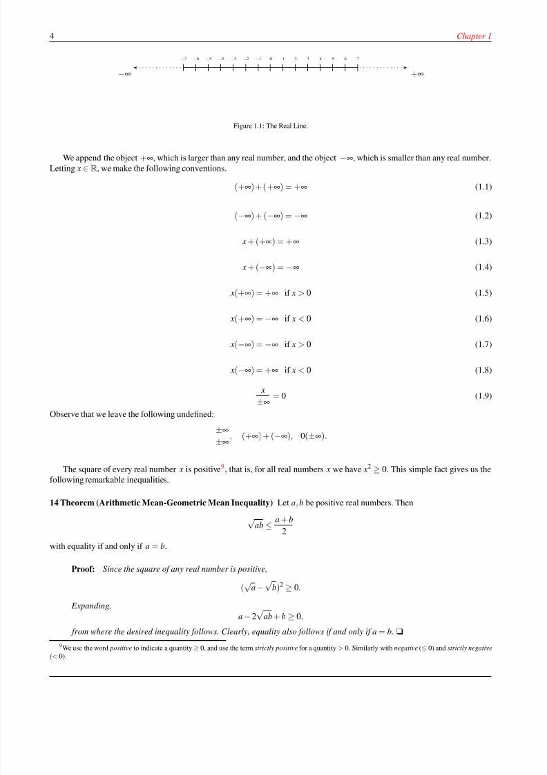
Geometrically, each real number can be viewed as a point on a straight line. We make the convention that we orient the real
line with 0 as the origin, the positive numbers increasing towards the right from 0 and the negative numbers decreasing towards
the left of 0, as in figure 1.1.
8/8/2019 Pre Calculus I
http://slidepdf.com/reader/full/pre-calculus-i 10/125
4 Chapter 1
0 1 2 3 4 5 6 7−1−2−3−4−5−6−7
+∞−∞
Figure 1.1: The Real Line.
We append the object +∞, which is larger than any real number, and the object −∞, which is smaller than any real number.
Letting x ∈ R, we make the following conventions.
(+∞) +( +∞) = +∞ (1.1)
(−∞) + (−∞) = −∞ (1.2)
x + (+∞) = +∞ (1.3)
x + (−∞) = −∞ (1.4)
x(+∞) = +∞ if x > 0 (1.5)
x(+∞) = −∞ if x < 0 (1.6)
x(−∞) = −∞ if x > 0 (1.7)
x(−∞) = +∞ if x < 0 (1.8)
x
±∞= 0 (1.9)
Observe that we leave the following undefined:
±∞±∞ , (+∞) + (−∞), 0(±∞).
The square of every real number x is positive9, that is, for all real numbers x we have x2 ≥ 0. This simple fact gives us the
following remarkable inequalities.
14 Theorem (Arithmetic Mean-Geometric Mean Inequality) Let a, b be positive real numbers. Then
√ab ≤ a + b
2
with equality if and only if a = b.
Proof: Since the square of any real number is positive,
(√
a −√
b)2 ≥ 0.
Expanding,
a − 2√
ab + b ≥ 0,
from where the desired inequality follows. Clearly, equality also follows if and only if a= b. u
9We use the word positive to indicate a quantity ≥ 0, and use the term strictly positive for a quantity > 0. Similarly with negative (≤ 0) and strictly negative
(< 0).
8/8/2019 Pre Calculus I
http://slidepdf.com/reader/full/pre-calculus-i 11/125
The Real Line 5
15 Corollary (Harmonic Mean-Geometric Mean Inequality) Let a, b be strictly positive real numbers. Then
21a
+ 1b
≤√
ab
with equality if and only if a = b.
Proof: By the Arithmetic Mean-Geometric Mean Inequality 1
a· 1
b≤
1a
+ 1b
2,
whence the desired result follows upon rearrangement. Clearly, equality also follows if and only if a= b. u
16 Example The sum of two positive real numbers is 50. Find their maximum product.
Let x, y be these positive real numbers with x + y = 50. By the Arithmetic Mean-Geometric Mean Inequality
√ xy ≤ x + y
2= 25.
Thus their maximum product is 625, since
xy ≤ 252 = 625.
Introducing the object i =√−1—whose square satisfies i2 = −1, a negative number—and considering the numbers of the
form a + bi, with a and b real numbers, we obtain the complex numbersC. The addition and multiplication of complex numbers
a + bi and c + di, where a, b, c, d are real numbers, is defined thus
(a + bi) + (c + di) = (a + c) + (b + d )i; (a + bi)(c + di) = (ac − bd ) + (ad + bc)i.
In summary we have
N
⊆Z
⊆Q
⊆R
⊆C.
Homework
17 Problem Give examples, if at all possible, of the following.
the sum of two ratio-
nals giving an irrational
number.
the sum of two irra-
tionals giving an irra-
tional number.
the sum of two irra-
tionals giving a rationalnumber.
the product of a rational
and an irrational giving
an irrational number.
the product of a rational
and an irrational giving
a rational number.
the product of two ir-
rationals giving an irra-
tional number. the product of two irra-
tionals giving a rational
number.
18 Problem Describe the following sets explicitly by either provid-
ing a list of their elements or an interval.
{ x ∈R : x3 = 8} { x ∈R : | x|3 = 8} { x ∈R : | x| = −8} { x ∈R : | x| < 4}
{ x ∈ Z : | x| < 4} { x ∈R : | x| < 1} { x ∈ Z : | x| < 1} { x ∈ Z : x2002 < 0}
19 Problem Describe explicitly the set { x ∈ Z : x < 0,1000 < x2 <2003} by listing its elements.
20 Problem Write the infinitely repeating decimal 0.123 =0.123123123 . . . as the quotient of two positive integers.
21 Problem Compute (123456789)2 − (123456791)(123456787)mentally.
22 Problem Describe explicitly the set
{ x ∈ Z : −13 ≤ x ≤ 15, x is divisible by 3}
by listing its elements.
23 Problem (Inclusion-Exclusion) Let X be a finite set and let
card ( X ) denote the number of elements of X . Prove that if A and B
are finite sets then card ( A∪ B) = card( A) + card ( B) −card( A∩ B).
8/8/2019 Pre Calculus I
http://slidepdf.com/reader/full/pre-calculus-i 12/125
6 Chapter 1
24 Problem Of 40 people, 28 smoke and 16 chew tobacco. It is also
known that 10 both smoke and chew. How many among the 40 nei-
ther smoke nor chew?
25 Problem Prove that if a, b, c are positive real numbers then
(a + b)(b + c)(c + a) ≥ 8abc.
26 Problem If a, b, c, d , are real numbers such that a2 + b2 + c2 +d 2 = ab + bc + cd + da, prove that a = b = c = d .
27 Problem The values of a, b, c, and d are 1,2,3 and 4 but not
necessarily in that order. What is the largest possible value of
ab + bc + cd + da?
28 Problem Prove that if r ≥ s ≥ t then
r 2 − s2 + t 2 ≥ (r − s + t )2
29 Problem Prove that
a3 + b3 + c3 − 3abc = (a + b + c)(a2 + b2 + c2 − ab− bc− ca)
and that
2a2 + 2b2 + 2c2 − 2ab− 2bc− 2ca = (a−b)2 + (b− c)2 + (c −a)2.
Deduce now the arithmetic-mean-geometric-mean inequality for
three positive real numbers, that is, prove that if α ≥ 0, β ≥ 0, γ ≥ 0,
then3 αβ γ ≤ α +β +γ
3.
1.2 Intervals
30 Definition An interval I is a subset of the real numbers with the following property: if s ∈ I and t ∈ I , and if s < x < t , then x ∈ I . In other words, intervals are those subsets of real numbers with the property that every number between two elements is
also contained in the set. Since there are infinitely many decimals between two different real numbers, intervals with distinct
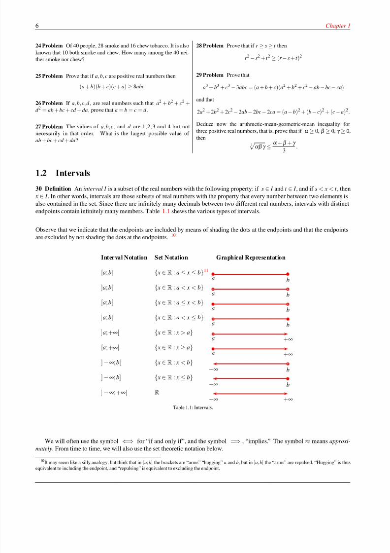
endpoints contain infinitely many members. Table 1.1 shews the various types of intervals.
Observe that we indicate that the endpoints are included by means of shading the dots at the endpoints and that the endpoints
are excluded by not shading the dots at the endpoints. 10
Interval Notation Set Notation Graphical Representation
[a; b] { x ∈ R : a ≤ x ≤ b}11
a b
]a; b[ { x ∈ R : a < x < b}a b
[a; b[ { x ∈ R : a ≤ x < b}a b
]a; b] { x ∈ R : a < x ≤ b}a b
]a; +∞[ { x ∈ R : x > a}a +∞
[a; +∞[ { x ∈ R : x ≥ a}a +∞
]−∞; b[ { x ∈ R : x < b}−∞ b
]
−∞; b]
{ x
∈R : x
≤b
} −∞ b
]−∞; +∞[ R−∞ +∞
Table 1.1: Intervals.
We will often use the symbol ⇐⇒ for “if and only if”, and the symbol =⇒ , “implies.” The symbol ≈ means approxi-
mately. From time to time, we will also use the set theoretic notation below.
10It may seem like a silly analogy, but think that in [a; b] the brackets are “arms” “hugging” a and b, but in ]a; b[ the “arms” are repulsed. “Hugging” is thusequivalent to including the endpoint, and “repulsing” is equivalent to excluding the endpoint.
8/8/2019 Pre Calculus I
http://slidepdf.com/reader/full/pre-calculus-i 13/125
Intervals 7
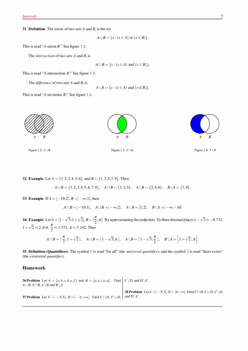
31 Definition The union of two sets A and B, is the set
A ∪ B = { x : ( x ∈ A) or ( x ∈ B)}.
This is read “ A union B.” See figure 1.2.
The intersection of two sets A and B, is
A ∩ B = { x : ( x ∈ A) and ( x ∈ B)}.
This is read “ A intersection B.” See figure 1.3.
The difference of two sets A and B, is
A \ B = { x : ( x ∈ A) and ( x ∈ B)}.
This is read “ A set minus B.” See figure 1.4.
A B
Figure 1.2: A ∪ B
A B
Figure 1.3: A ∩ B
A B
Figure 1.4: A \ B
32 Example Let A =
{1, 2, 3, 4, 5, 6
}, and B =
{1, 3, 5, 7, 9
}. Then
A ∪ B = {1, 2, 3, 4, 5, 6, 7, 9}, A ∩ B = {1, 3, 5}, A \ B = {2, 4, 6}, B \ A = {7, 9}.
33 Example If A = [−10;2], B =] −∞; 1[, then
A ∩ B = [−10;1[, A ∪ B =] −∞; 2], A \ B = [1; 2], B \ A =] −∞;−10[
34 Example Let A = [1−√
3; 1+√
2], B = [π
2;π [. By approximating the endpoints. To three decimal places 1−
√3 ≈ −0.732,
1 +√
2 ≈ 2.414,π
2≈ 1.571, π ≈ 3.142. Thus
A
∩ B = [
π
2
; 1 +√
2 ] , A
∪ B = [ 1
−
√3;π [ , A
\ B = [ 1
−
√3;
π
2
[ , B
\ A = 1 +
√2 ; π .
35 Definition (Quantifiers) The symbol ∀ is read “for all” (the universal quantifier ), and the symbol ∃ is read “there exists”
(the existential quantifier ).
Homework
36 Problem Let A = {a, b, c, d , e, f } and B = {a, e, i, o, u}. Find
A∪ B, A ∩ B, A \ B and B\ A.
37 Problem Let C =] − 5; 5[, D =] − 1; +∞[. Find C ∩ D, C ∪ D,
C \ D, and D\C .
38 Problem Let C =]−5; 3[, D = [4; +∞[. Find C ∩ D, C ∪ D, C \ D,
and D\C .
8/8/2019 Pre Calculus I
http://slidepdf.com/reader/full/pre-calculus-i 14/125
8 Chapter 1
39 Problem Let C = [−1;−2 +√
3[, D = [−0.5;√
2 − 1]. Find C ∩ D, C ∪ D, C \ D, and D\C .
1.3 Sets on the Plane
40 Definition Let A1, A2, . . . , An, be sets. The Cartesian Product of these n sets is defined and denoted by
A1 × A2 ×· · ·× An = {(a1, a2, . . . ,an) : ak ∈ Ak },
that is, the set of all ordered n-tuples whose elements belong to the given sets.
! In the particular case when all the Ak are equal to a set A, we write
A1 × A2 ×· · ·× An = An.
41 Example If A = {−1,−2} and B = {−1, 2} then
A × B = {(−1,−1), (−1, 2), (−2,−1), (−2, 2))},
B × A = {(−1,−1), (−1,−2), (2,−1), (2,−2)},
A2 = {(−1,−1), (−1,−2), (−2,−1), (−2,−2)},
B2 = {(−1,−1), (−1, 2), (2,−1), (2, 2)}.
Notice that these sets are all different, even though some elements are shared.
42 Example (−1, 2) ∈ Z2 but (−1,√
2) ∈ Z2.
43 Example (−1,√
2) ∈ Z×R but (−1,√
2) ∈ R×Z.
44 Definition R2 =R
×R—the real Cartesian Plane—- is the set of all ordered pairs ( x, y) of real numbers.
We represent the elements of R2 graphically as follows. Intersect perpendicularly two copies of the real number line. These
two lines are the axes. Their point of intersection—which we label O = (0, 0)— is the origin. To each point P on the plane we
associate an ordered pair P = ( x, y) of real numbers. Here x is the abscissa12, which measures the horizontal distance of our
point to the origin, and y is the ordinate, which measures the vertical distance of our point to the origin. The points x and y are
the coordinates of P. This manner of dividing the plane and labelling its points is called the Cartesian coordinate system. The
horizontal axis is called the x-axis and the vertical axis is called the y-axis. It is therefore sufficient to have two numbers x and
y to completely characterise the position of a point P = ( x, y) on the plane R2.
1
2
3
4
−1
−2
−3
−4
1 2 3 4−1−2−3−4
Figure 1.5: Example 45.
1
2
3
4
−1
−2
−3
−4
1 2 3 4−1−2−3−4
Figure 1.6: Example 46
.
1
2
3
4
−1
−2
−3
−4
1 2 3 4−1−2−3−4
Figure 1.7: Example 47.
D
C B
A
E F G
Figure 1.8: Example 48.
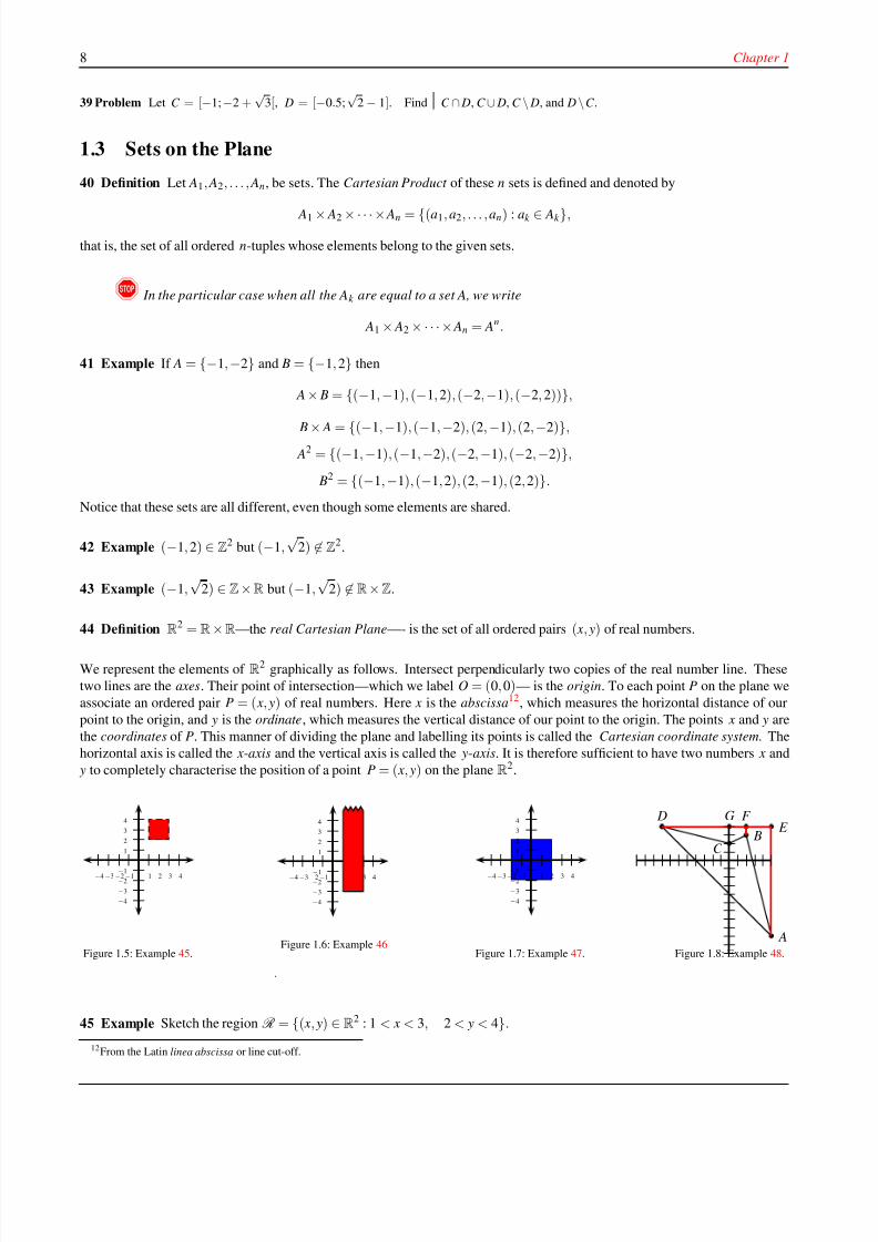
45 Example Sketch the region R = {( x, y) ∈ R2 : 1 < x < 3, 2 < y < 4}.
12From the Latin linea abscissa or line cut-off.
8/8/2019 Pre Calculus I
http://slidepdf.com/reader/full/pre-calculus-i 15/125
Neighbourhood of a point 9
Solution: The region is a square, excluding its boundary. The graph is shewn in figure 1.5, where we have dashed the boundary
lines in order to represent their exclusion.
46 Example The region R = [1; 3] × [−3; +∞[ is the infinite half strip on the plane sketched in figure 1.6. The boundary
lines are solid, to indicate their inclusion. The upper boundary line is toothed, to indicate that it continues to infinity.
47 Example The region R
= {( x, y) ∈ R2
: | x| ≤ 2, | y| ≤ 2} is the 4 × 4 square sketched in figure 1.7.
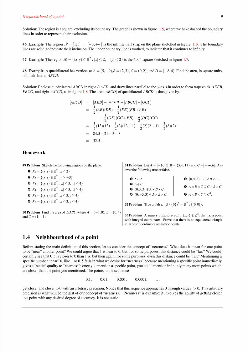
48 Example A quadrilateral has vertices at A = (5,−9), B = (2, 3), C = (0, 2), and D = (−8, 4). Find the area, in square units,
of quadrilateral ABCD.
Solution: Enclose quadrilateral ABCD in right △ AED, and draw lines parallel to the y-axis in order to form trapezoids AEFB,
FBCG, and right △GCD, as in figure 1.8. The area [ ABCD] of quadrilateral ABCD is thus given by
[ ABCD] = [ AED]− [ AEFB]− [FBCG]− [GCD]
=1
2( AE )( DE ) − 1
2(FE )(FB + AE )−
−1
2
(GF )(GC + FB)
−1
2
( DG)(GC )
=1
2(13)(13) − 1
2(3)(13 + 1) − 1
2(2)(2 + 1) − 1
2(8)(2)
= 84.5 − 21 − 3 − 8
= 52.5.
Homework
49 Problem Sketch the following regions on the plane.
R1 = {( x, y) ∈ R2 : x ≤ 2} R2 = {( x, y) ∈ R2 : y ≥ −3} R3 = {( x, y) ∈ R2 : | x| ≤ 3, | y| ≤ 4} R4 = {( x, y) ∈ R2 : | x| ≤ 3, | y| ≥ 4} R5 = {( x, y) ∈ R2 : x ≤ 3, y ≥ 4} R6 = {( x, y) ∈ R2 : x ≤ 3, y ≤ 4}
50 Problem Find the area of △ ABC where A = (−1, 0), B = (0, 4)and C = (1,−1).
51 Problem Let A = [−10;5], B = {5,6, 11} and C =] −∞; 6[. An-
swer the following true or false.
5
∈ A.
6 ∈ C .
(0, 5,3) ∈ A × B ×C .
(0,−5, 3) ∈ A× B×C .
(0, 5,3)
∈C
× B
×C .
A × B ×C ⊆ C × B ×C .
A × B ×C ⊆ C 3.
52 Problem True or false: (R\{0})2 =R2 \{(0, 0)}.
53 Problem A lattice point is a point ( x, y) ∈ Z2, that is, a point
with integral coordinates. Prove that there is no equilateral triangle
all whose coordinates are lattice points.
1.4 Neighbourhood of a point
Before stating the main definition of this section, let us consider the concept of “nearness.” What does it mean for one point
to be “near” another point? We could argue that 1 is near to 0, but, for some purposes, this distance could be “far.” We could
certainly see that 0.5 is closer to 0 than 1 is, but then again, for some purposes, even this distance could be “far.” Mentioning a
specific number “near” 0, like 1 or 0.5 fails in what we desire for “nearness” because mentioning a specific point immediately
gives a “static” quality to “nearness”: once you mention a specific point, you could mention infinitely many more points which
are closer than the point you mentioned. The points in the sequence
0.1, 0.01, 0.001, 0.0001, . . .
get closer and closer to 0 with an arbitrary precision. Notice that this sequence approaches 0 through values > 0. This arbitrary
precision is what will be the gist of our concept of “nearness.” “Nearness” is dynamic: it involves the ability of getting closer
to a point with any desired degree of accuracy. It is not static.
8/8/2019 Pre Calculus I
http://slidepdf.com/reader/full/pre-calculus-i 16/125
10 Chapter 1
Again, the points in the sequence
−1
2, −1
4, −1
8, − 1
16, . . .
are arbitrarily close to 0, but they “approach” 0 from the left. Once again, the sequence
+
1
2 , −1
3 , +
1
4 , −1
5 , . . .
approaches 0 from both above and below. After this long preamble, we may formulate our first definition.
54 Definition The notation x → a, read “ x tends to a,” means that x is very close, with an arbitrary degree of precision, to
a. Here x can approach a through values smaller or larger than a. We write x → a+ (read “ x tends to a from the right”) to
mean that x approaches a through values larger than a and we write x → a− (read “ x tends to a from the left”) we mean that x
approaches a through values smaller than a.
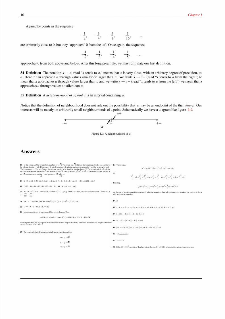
55 Definition A neighbourhood of a point a is an interval containing a.
Notice that the definition of neighbourhood does not rule out the possibility that a may be an endpoint of the the interval. Our
interests will be mostly on arbitrarily small neighbourhoods of a point. Schematically we have a diagram like figure 1.9.
−∞ +∞a
a+
a−|
Figure 1.9: A neighbourhood of a.
Answers
17 1) this is impossible. 2) take both numbers to be
√2. Their sum is 2
√2 which is also irrational. 3) take one number tobe √2 and the other −√2. Their sum is 0, which is rational. 4) take the rational number to be 1 and the irrational to be √2.
Their product is 1 ·√
2 =√
2. 5) take the rational number to be 0 and the irrational to be√
2. Their product is 0 ·√
2 = 0. 6)
take one irrational number to be√
2 and the other to be√
3. Their product is√
2 ·√
3 =√
6. 7) take one irrational number to
be√
2 and the other to be1√
2. Their product is
√2 · 1√
2= 1.
18 (i) {2}, (ii) {−2, 2}, (iii) ∅, (iv) ] −4;4 [, (v) {−3,−2,−1, 0, 1, 2, 3}, (vi) ] −1;1 [, (vii) {0}, (viii) ∅
19 {−32,−33,−34, −35,−36, −37,−38,−39, −40,−41,−42,−43,−44}
20 If x = 0.123123123 .. . then 1000 x = 0.123123123 .. . giving 1000 x − x = 123, since the tails cancel out. This results in
x =123
999=
41
333.
21 Put x = 123456789. Then we want x2 − ( x − 2)( x + 2) = x2 − ( x2 −4) = 4.
22 {−12,−9,−6,−3, 0, 3, 6, 9, 12, 15}
24 Let A denote the set of smokers and B the set of chewers. Then
card ( A ∪ B) = card ( A) + card ( B) −card ( A∩ B) = 28 + 16 −10 = 34,
meaning that there are 34 people that either smoke or chew (or possibly both). Therefore the number of people that neither
smoke nor chew is 40 − 34 = 6.
25 The result quickly follows upon multiplying the three inequalities
a + b ≥ 2√
ab,
b + c ≥ 2√
bc,
c + a ≥ 2√
ca.
26 Transposing,a2 − ab + b2 −bc + c2 − dc + d 2 − da = 0,
or
a2
2− ab +
b2
2+
b2
2− bc +
c2
2+
c2
2−dc +
d 2
2+
d 2
2− da +
a2
2= 0.
Factoring,
1
2(a− b)2 +
1
2(b −c)2 +
1
2(c− d )2 +
1
2(d −a)2 = 0.
As the sum of positive quantities is zero only when the quantities themselves are zero, we obtain a = b, b = c, c = d , d = a,which proves the assertion.
27 25
36 A∪ B = {a, b, c, d , e, f , i, o, u}, A∩ B = {a, e}, A \ B = {b, c, d , f }, B \ A = {i, o, u}
37 ]− 1;5 [, ]− 5; +∞[, ]− 5;−1], [5; +∞[
38 ∅, ]− 5;3 [∪[4; +∞[, ]− 5;3 [, [4; +∞[
39 [−0.5;−2 +√
3[, [−1;√
2− 1], [−1;−0.5[, [−2 +√
3;√
2 −1]
50 4.5 square units.
51 TFTFTTF
52 False. (R\{0})2 consists of the plane minus the axes.R2 \{ (0, 0)} consists of the plane minus the origin.
8/8/2019 Pre Calculus I
http://slidepdf.com/reader/full/pre-calculus-i 17/125
Chapter
2Distance and Curves on the Plane
The main objective of this chapter is to introduce the distance formula for two points on the plane, and by means of this distance
formula, the linking of certain equations with certain curves on the plane. Thus the main object of these notes, that of relating
a graph to a formula, is partially answered.
2.1 Distance on the Real Line
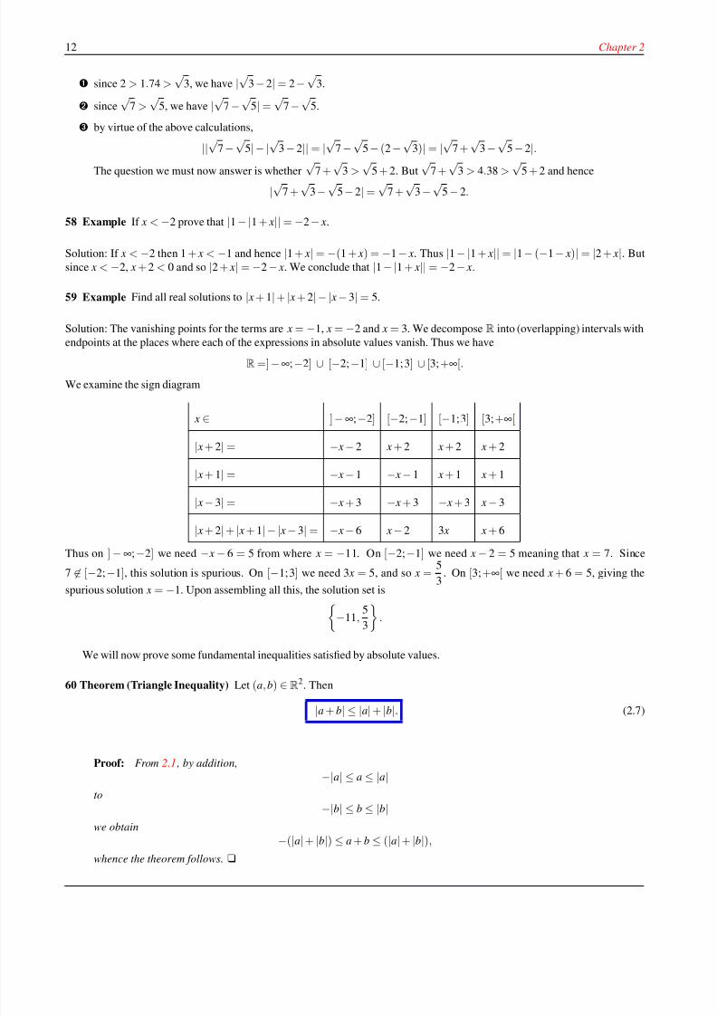
56 Definition Let x ∈ R. The absolute value of x—denoted by | x|—is defined by
| x| =
− x if x < 0,
x if x ≥ 0.
The absolute value of a real number is thus the distance of that real number to 0, and hence | x− y| is the distance between x and
y on the real line. Below are some properties of the absolute value. Here x, y,t are all real numbers.
−| x| ≤ x ≤ | x|. (2.1)
| x − y| = | y − x| (2.2)
√ x2 = | x| (2.3)
| x|2 = | x2| = x2 (2.4)
| x
| ≤t
⇐⇒ −t
≤ x
≤t (t
≥0) (2.5)
| x| ≥ t ⇐⇒ x ≤ −t or x ≥ t (t ≥ 0) (2.6)
57 Example Write without absolute value signs:
|√
3 − 2|, |
√7 −
√5|,
||√
7 −√
5|− |√
3− 2||
Solution: We have
11
8/8/2019 Pre Calculus I
http://slidepdf.com/reader/full/pre-calculus-i 18/125
12 Chapter 2
since 2 > 1.74 >√
3, we have |√
3 − 2| = 2 −√
3.
since√
7 >√
5, we have |√
7 −√
5| =√
7 −√
5.
by virtue of the above calculations,
||√
7 −√
5|− |√
3 − 2|| = |√
7 −√
5 − (2 −√
3)| = |√
7 +√
3 −√
5 − 2|.
The question we must now answer is whether
√7 +
√3 >
√5 + 2. But
√7 +
√3 > 4.38 >
√5 + 2 and hence
|√
7 +√
3−√
5 − 2| =√
7 +√
3 −√
5 − 2.
58 Example If x < −2 prove that |1 −|1 + x|| = −2 − x.
Solution: If x < −2 then 1 + x < −1 and hence |1 + x| = −(1 + x) = −1 − x. Thus |1 −|1 + x|| = |1− (−1 − x)| = |2 + x|. But
since x < −2, x + 2 < 0 and so |2 + x| = −2 − x. We conclude that |1 −|1 + x|| = −2 − x.
59 Example Find all real solutions to | x + 1|+ | x + 2|− | x − 3| = 5.
Solution: The vanishing points for the terms are x = −1, x = −2 and x = 3. We decompose R into (overlapping) intervals with
endpoints at the places where each of the expressions in absolute values vanish. Thus we have
R=] −∞;−2] ∪ [−2;−1] ∪ [−1; 3] ∪ [3; +∞[.
We examine the sign diagram
x ∈ ]−∞;−2] [−2;−1] [−1; 3] [3; +∞[
| x + 2| = − x − 2 x + 2 x + 2 x + 2
| x + 1| = − x − 1 − x − 1 x + 1 x + 1
| x− 3| = − x + 3 − x + 3 − x + 3 x − 3
| x + 2| + | x + 1|− | x − 3| = − x − 6 x − 2 3 x x + 6
Thus on ] −∞;−2] we need − x − 6 = 5 from where x = −11. On [−2;−1] we need x − 2 = 5 meaning that x = 7. Since
7 ∈ [−2;−1], this solution is spurious. On [−1; 3] we need 3 x = 5, and so x =5
3. On [3; +∞[ we need x + 6 = 5, giving the
spurious solution x = −1. Upon assembling all this, the solution set is−11,
5
3
.
We will now prove some fundamental inequalities satisfied by absolute values.
60 Theorem (Triangle Inequality) Let (a, b) ∈ R2. Then
|a + b| ≤ |a| + |b|. (2.7)
Proof: From 2.1 , by addition,
−|a| ≤ a ≤ |a|to
−|b| ≤ b ≤ |b|we obtain
−(|a|+ |b|) ≤ a + b ≤ (|a| + |b|),
whence the theorem follows. u
8/8/2019 Pre Calculus I
http://slidepdf.com/reader/full/pre-calculus-i 19/125
Distance on the Real Plane 13
61 Corollary Let (a, b) ∈ R2. Then
||a|− |b| |≤ |a − b| . (2.8)
Proof: We have
|a| = |a − b + b| ≤ |a − b| + |b|,giving
|a|− |b| ≤ |a − b|.Similarly,
|b| = |b − a + a| ≤ |b − a| + |a| = |a − b| + |a|,gives
|b|− |a| ≤ |a − b|.The stated inequality follows from this.u
Homework
62 Problem Write without absolute values: |√
3 −
|2 −√
15| |
63 Problem Write without absolute values if x > 2: | x −|1− 2 x||.
64 Problem Find all the real solutions to |5 x −2| = |2 x + 1|.
65 Problem Find all real solutions to | x− 2|+ | x − 3| = 1.
66 Problem Find the set of solutions to the equation | x|+ | x−1| = 2.
67 Problem Find the solution set to the equation | x|+ | x −1| = 1.
68 Problem Find thesolution setto theequation |2 x|+| x−1|−3| x+2| = 1.
69 Problem Find thesolution setto theequation |2 x|+| x−1|−3| x+2| = −7.
70 Problem Find thesolution setto theequation |2 x|+| x−1|−3| x+2| = 7.
71 Problem If x < 0 prove that
x −
( x −1)2
= 1− 2 x.
72 Problem Find the real solutions, if any, to | x2 −3 x| = 2.
73 Problem Find the real solutions, if any, to x2 − 2| x|+ 1 = 0.
74 Problem Find the real solutions, if any, to x2 −| x|− 6 = 0.
75 Problem Find the real solutions, if any, to x2 = |5 x −6|.
76 Problem Prove that if x ≤ −3, then | x + 3|− | x −4| is constant.
77 Problem Prove that max(a, b) =a + b + |a −b|
2.
78 Problem Prove that min(a, b) =a + b −|a −b|
2.
2.2 Distance on the Real PlaneWe now turn our attention to the plane, which we denote by the symbol R2.
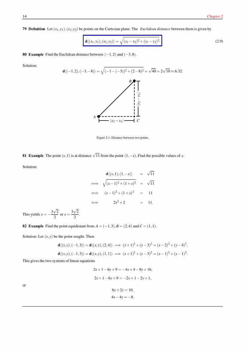
Consider two points A = ( x1, y1), B = ( x2, y2) on the Cartesian plane, as in figure 2.1. Dropping perpendicular lines to C , as
in the figure, we can find their Euclidean distance AB with the aid of the Pythagorean Theorem. For
AB2 = AC 2 + BC 2,
translates into
AB =
( x2 − x1)2 + ( y2 − y1)2.
This motivates the following definition.
8/8/2019 Pre Calculus I
http://slidepdf.com/reader/full/pre-calculus-i 20/125
14 Chapter 2
79 Definition Let ( x1, y1), ( x2, y2) be points on the Cartesian plane. The Euclidean distance between them is given by
d( x1, y1), ( x2, y2) =
( x1 − x2)2 + ( y1 − y2)2. (2.9)
80 Example Find the Euclidean distance between (−1, 2) and (−3, 8).
Solution:
d(−1, 2), (−3,−8) =
(−1 − (−3))2 + (2 − 8)2 =√
40 = 2√
10 ≈ 6.32.
A
B
C
| y 2
−
y 1
|
| x2 − x1|
Figure 2.1: Distance between two points.
81 Example The point ( x, 1) is at distance√
11 from the point (1,− x). Find the possible values of x.
Solution:
d( x, 1), (1,− x) =√
11
⇐⇒ ( x− 1)2 + (1 + x)2 = √11
⇐⇒ ( x − 1)2 + (1 + x)2 = 11
⇐⇒ 2 x2 + 2 = 11.
This yields x = −3√
2
2or x =
3√
2
2.
82 Example Find the point equidistant from A = (−1, 3), B = (2, 4) and C = (1, 1).
Solution: Let ( x, y) be the point sought. Then
d( x, y), (−1, 3) = d( x, y), (2, 4) =⇒ ( x + 1)2 + ( y − 3)2 = ( x − 2)2 + ( y− 4)2,
d( x, y), (−1, 3) = d( x, y), (1, 1) =⇒ ( x + 1)2 + ( y − 3)2 = ( x − 1)2 + ( y− 1)2.
This gives the two systems of linear equations
2 x + 1− 6 y + 9 = −4 x + 4 − 8 y + 16,
2 x + 1 − 6 y + 9 = −2 x + 1 − 2 y + 1,
or
6 x + 2 y = 10,
4 x − 4 y = −8.
8/8/2019 Pre Calculus I
http://slidepdf.com/reader/full/pre-calculus-i 21/125
Distance on the Real Plane 15
This system solves to ( x, y) = (3
4,
11
4).
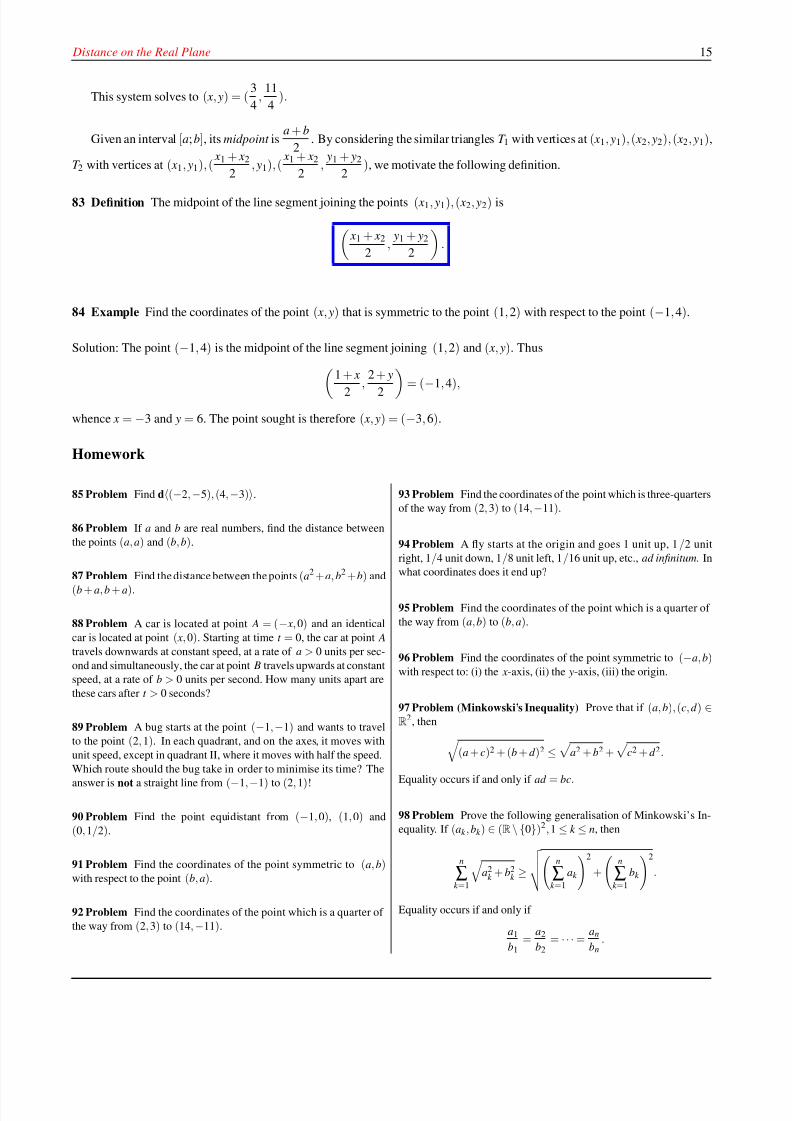
Given an interval [a; b], its midpoint isa + b
2. By considering the similar triangles T 1 with vertices at ( x1, y1), ( x2, y2), ( x2, y1),
T 2 with vertices at ( x1, y1), ( x1 + x2
2, y1), (
x1 + x2
2,
y1 + y2
2), we motivate the following definition.
83 Definition The midpoint of the line segment joining the points ( x1, y1), ( x2, y2) is
x1 + x2
2,
y1 + y2
2
.
84 Example Find the coordinates of the point ( x, y) that is symmetric to the point (1, 2) with respect to the point (−1, 4).
Solution: The point (−1, 4) is the midpoint of the line segment joining (1, 2) and ( x, y). Thus
1 + x
2 ,
2 + y
2 = (−1, 4),
whence x = −3 and y = 6. The point sought is therefore ( x, y) = (−3, 6).
Homework
85 Problem Find d(−2,−5), (4,−3).
86 Problem If a and b are real numbers, find the distance between
the points (a, a) and (b, b).
87 Problem Find the distance between the points(
a2
+a
,b2
+b
)and
(b + a, b + a).
88 Problem A car is located at point A = (− x, 0) and an identical
car is located at point ( x, 0). Starting at time t = 0, the car at point A
travels downwards at constant speed, at a rate of a > 0 units per sec-
ond and simultaneously, the car at point B travels upwards at constant
speed, at a rate of b > 0 units per second. How many units apart are
these cars after t > 0 seconds?
89 Problem A bug starts at the point (−1,−1) and wants to travel
to the point (2, 1). In each quadrant, and on the axes, it moves with
unit speed, except in quadrant II, where it moves with half the speed.
Which route should the bug take in order to minimise its time? The
answer is not a straight line from (−1,−1) to (2, 1)!
90 Problem Find the point equidistant from (−1, 0), (1, 0) and
(0,1/2).
91 Problem Find the coordinates of the point symmetric to (a, b)with respect to the point (b, a).
92 Problem Find the coordinates of the point which is a quarter of
the way from (2, 3) to (14,−11).
93 Problem Find the coordinates of the point which is three-quarters
of the way from (2, 3) to (14,−11).
94 Problem A fly starts at the origin and goes 1 unit up, 1/2 unit
right, 1/4 unit down, 1/8 unit left, 1/16 unit up, etc., ad infinitum. In
what coordinates does it end up?
95 Problem Find the coordinates of the point which is a quarter of
the way from (a, b) to (b, a).
96 Problem Find the coordinates of the point symmetric to (−a, b)with respect to: (i) the x-axis, (ii) the y-axis, (iii) the origin.
97 Problem (Minkowski’s Inequality) Prove that if (a, b),(c, d ) ∈R2, then
(a + c)2 + (b + d )2 ≤
a2 + b2 +
c2 + d 2.
Equality occurs if and only if ad = bc.
98 Problem Prove the following generalisation of Minkowski’s In-
equality. If (ak , bk ) ∈ (R\{0})2,1 ≤ k ≤ n, then
n
∑k =1
a2
k + b2
k ≥
n
∑k =1
ak
2
+
n
∑k =1
bk
2
.
Equality occurs if and only if
a1
b1=
a2
b2= · · · =
an
bn.
8/8/2019 Pre Calculus I
http://slidepdf.com/reader/full/pre-calculus-i 22/125
16 Chapter 2
99 Problem (AIME 1991) Let P = {a1, a2, . . . , an} be a collection
of points with
0 < a1 < a2 < · · · < an < 17.
Consider
Sn = minP
n
∑k =1
(2k −1)2 + a2
k ,
where the minimum runs over all such partitions P. Shew that exactly
one of S2, S3, . . . ,Sn, . . . is an integer, and find which one it is.
2.3 Circles
We now study our first curve on the plane: the circle. We will see that the equation of a circle on the plane is a consequence of
the distance formula 2.9.
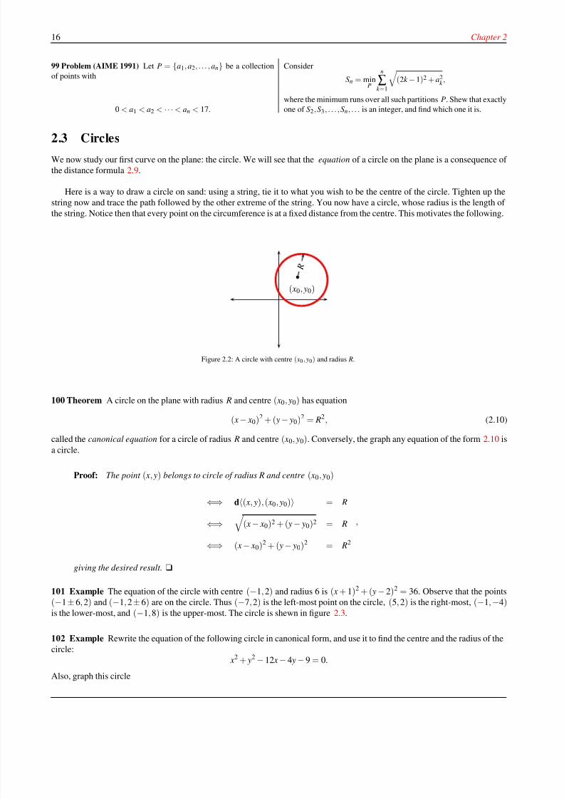
Here is a way to draw a circle on sand: using a string, tie it to what you wish to be the centre of the circle. Tighten up the
string now and trace the path followed by the other extreme of the string. You now have a circle, whose radius is the length of
the string. Notice then that every point on the circumference is at a fixed distance from the centre. This motivates the following.
( x0, y0)
R
Figure 2.2: A circle with centre ( x0, y0) and radius R.
100 Theorem A circle on the plane with radius R and centre ( x0, y0) has equation
( x− x0)2 + ( y− y0)2 = R2, (2.10)
called the canonical equation for a circle of radius R and centre ( x0, y0). Conversely, the graph any equation of the form 2.10 is
a circle.
Proof: The point ( x, y) belongs to circle of radius R and centre ( x0, y0)
⇐⇒ d( x, y), ( x0, y0) = R
⇐⇒
( x − x0)2 + ( y − y0)2 = R
⇐⇒( x
− x0)2 + ( y
− y0)2 = R2
,
giving the desired result. u
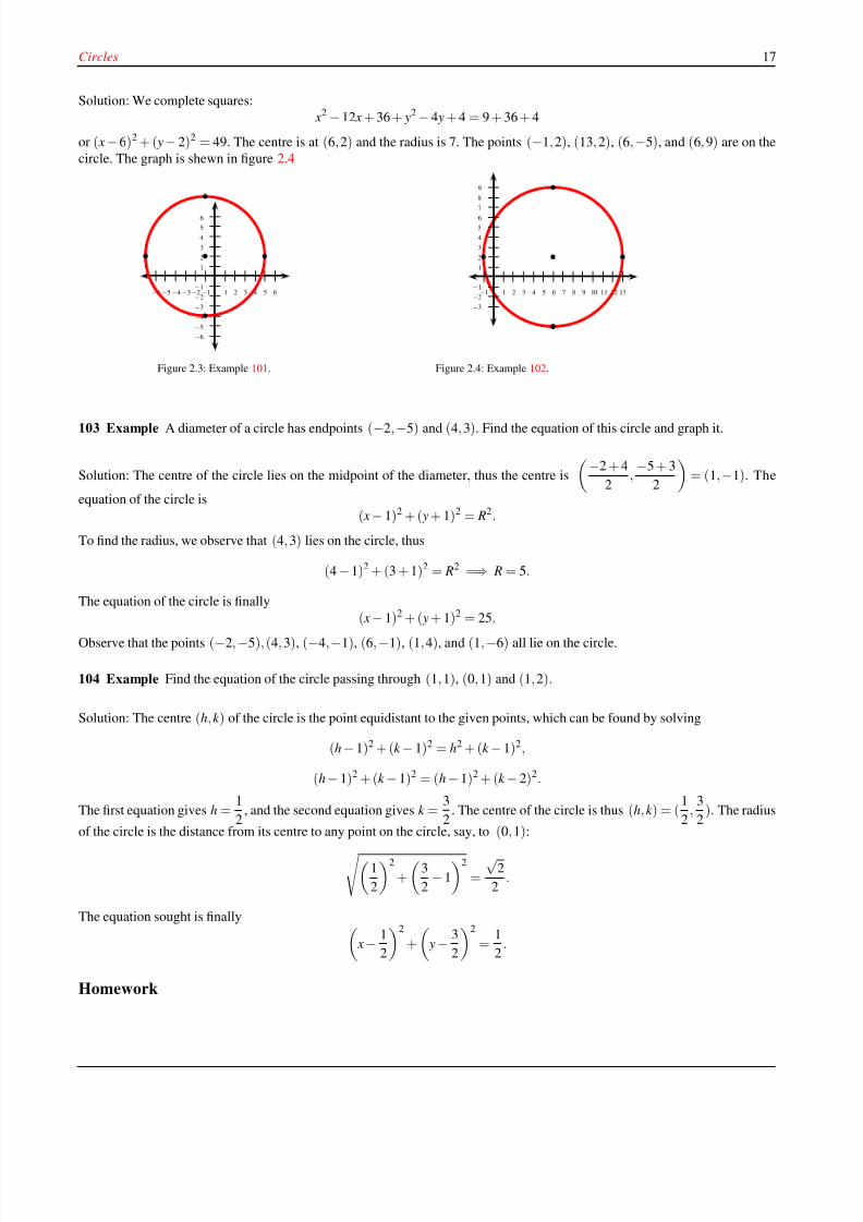
101 Example The equation of the circle with centre (−1, 2) and radius 6 is ( x + 1)2 + ( y − 2)2 = 36. Observe that the points
(−1± 6, 2) and (−1, 2± 6) are on the circle. Thus (−7, 2) is the left-most point on the circle, (5, 2) is the right-most, (−1,−4)is the lower-most, and (−1, 8) is the upper-most. The circle is shewn in figure 2.3.
102 Example Rewrite the equation of the following circle in canonical form, and use it to find the centre and the radius of the
circle:
x2 + y2 − 12 x − 4 y − 9 = 0.
Also, graph this circle
8/8/2019 Pre Calculus I
http://slidepdf.com/reader/full/pre-calculus-i 23/125
Circles 17
Solution: We complete squares:
x2 − 12 x + 36 + y2 − 4 y + 4 = 9 + 36 + 4
or ( x − 6)2 + ( y − 2)2 = 49. The centre is at (6, 2) and the radius is 7. The points (−1, 2), (13, 2), (6,−5), and (6, 9) are on the
circle. The graph is shewn in figure 2.4
1
2
3
4
5
6
−1
−2
−3
−4
−5
−6
1 2 3 4 5 6−1−2−3−4−5−6
Figure 2.3: Example 101.
1
2
3
4
5
67
8
9
−1
−2
−3
1 2 3 4 5 6 7 8 9 10 11 12 13−1
Figure 2.4: Example 102.
103 Example A diameter of a circle has endpoints (−2,−5) and (4, 3). Find the equation of this circle and graph it.
Solution: The centre of the circle lies on the midpoint of the diameter, thus the centre is
−2 + 4
2,−5 + 3
2
= (1,−1). The
equation of the circle is
( x − 1)2 + ( y + 1)2 = R2.
To find the radius, we observe that (4, 3) lies on the circle, thus
(4 − 1)2 + (3 + 1)2 = R2 =⇒ R = 5.
The equation of the circle is finally
( x
−1)2 + ( y + 1)2 = 25.
Observe that the points (−2,−5), (4, 3), (−4,−1), (6,−1), (1, 4), and (1,−6) all lie on the circle.
104 Example Find the equation of the circle passing through (1, 1), (0, 1) and (1, 2).
Solution: The centre (h, k ) of the circle is the point equidistant to the given points, which can be found by solving
(h − 1)2 + (k − 1)2 = h2 + (k − 1)2,
(h− 1)2 + (k − 1)2 = (h − 1)2 + (k − 2)2.
The first equation gives h =1
2, and the second equation gives k =
3
2. The centre of the circle is thus (h, k ) = (
1
2,
3
2). The radius
of the circle is the distance from its centre to any point on the circle, say, to (0, 1): 1
2
2
+
3
2− 1
2
=
√2
2.
The equation sought is finally x − 1
2
2
+
y− 3
2
2
=1
2.
Homework
8/8/2019 Pre Calculus I
http://slidepdf.com/reader/full/pre-calculus-i 24/125
18 Chapter 2
105 Problem Prove that the points (4, 2) and (−2,−6) lie on the cir-
cle with centre at (1,−2) and radius 5. Prove, moreover, that these
two points are diametrically opposite.
106 Problem A diameter AB of a circle has endpoints A = (1,2) and
B = (3,4). Find the equation of this circle.
107 Problem Find the equation of the circle with centre at (−1, 1)and passing through (1, 2).
108 Problem Rewrite the following circle equations in canonical
form and find their centres C and their radius R. Draw the circles.
Also, find at least four points belonging to each circle.
x2 + y2 −2 y = 35,
x2 + 4 x + y2 − 2 y = 20,
x2 + 4 x + y2 − 2 y = 5,
2 x2 −8 x + 2 y2 = 16,
4 x
2
+ 4 x +
15
2 + 4 y
2
−12 y = 0 3 x2 + 2 x
√3 + 5 + 3 y2 − 6 y
√3 = 0
109 Problem Let
R1 = {( x, y) ∈ R2| x2 + y2 ≤ 9},
R2 = {( x, y) ∈R2|( x + 2)2 + y2 ≤ 1},
R3 = {( x, y) ∈R2|( x − 2)2 + y2 ≤ 1},
R4 = {( x, y) ∈R2| x2 + ( y + 1)2 ≤ 1},
R5 = {( x, y) ∈R2|| x| ≤ 3, | y| ≤ 3},
R6 =
{( x, y)
∈R2
|| x
| ≥2,
| y
| ≥2
}.
Sketch the following regions.
R1 \ ( R2 ∪ R3 ∪ R4).
R5 \ R1
R1 \ R6
R2 ∪ R3 ∪ R6
110 Problem Find the equation of the circle passing through (−1, 2)and centre at (1, 3).
111 Problem Find the canonical equation of the circle passing
through (−1, 1), (1,−2), and (0, 2).
112 Problem Let a, b, c be real numbers with a2 > 4b. Construct a
circle with diameter at the points (1,0) and (−a, b). Shew that the
intersection of this circle with the x-axis are the roots of the equation
x2 + ax + b = 0. Why must we impose a2 > 4b?
2.4 Semicircles
Solving for y in ( x − x0)2 + ( y− y0)2 = R2, we obtain
y = y0
± R2
−( x
− x0)2.
The choice of the + sign gives the upper half of the circle (the upper semicircle) and the − sign gives the lower semicircle.
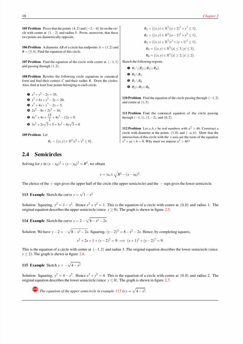
113 Example Sketch the curve y =
1 − x2
Solution: Squaring, y2 = 1 − x2. Hence x2 + y2 = 1. This is the equation of a circle with centre at (0, 0) and radius 1. The
original equation describes the upper semicircle (since y ≥ 0). The graph is shewn in figure 2.5.
114 Example Sketch the curve y = 2 −
8− x2 − 2 x
Solution: We have y − 2 = −
8 − x2 − 2 x. Squaring, ( y − 2)2 = 8− x2 − 2 x. Hence, by completing squares,
x2 + 2 x + 1 + ( y − 2)2 = 9 =⇒ ( x + 1)2 + ( y − 2)2 = 9.
This is the equation of a circle with centre at (−1, 2) and radius 3. The original equation describes the lower semicircle (since
y ≤ 2). The graph is shewn in figure 2.6.
115 Example Sketch y = −
4 − x2
Solution: Squaring, y2 = 4 − x2. Hence x2 + y2 = 4. This is the equation of a circle with centre at (0, 0) and radius 2. The
original equation describes the lower semicircle (since y ≤ 0). The graph is shewn in figure 2.7.
! The equation of the upper semicircle in example 115 is y =
4− x2.
8/8/2019 Pre Calculus I
http://slidepdf.com/reader/full/pre-calculus-i 25/125
Semicircles 19
Solving for x in ( x − x0)2 + ( y − y0)2 = R2, we obtain
x = x0 ±
R2 − ( y− y0)2.
The choice of the + sign gives the right half of the circle and the − sign gives the left semicircle.
116 Example Sketch the curve x = 4− y2
Solution: Squaring, x2 = 4 − y2. Hence x2 + y2 = 4. This is the equation of a circle with centre at (0, 0) and radius 2. The
original equation describes the right semicircle (since x ≥ 0). The graph is shewn in figure 2.8.
! The equation of the left semicircle in example 116 is x = −
4 − y2.
1
2
3
4
5
6
−1
−2
−3
−4
−5
−6
1 2 3 4 5 6−1−2−3−4−5−6
Figure 2.5: Example 113
1
2
3
4
5
6
−1
−2
−3
−4
−5
−6
1 2 3 4 5 6−1−2−3−4−5−6
Figure 2.6: Example 114
1
2
−1
−2
1 2−1−2
Figure 2.7: Example 115
1
2
−1
−2
1 2−1−2
Figure 2.8: Example 116
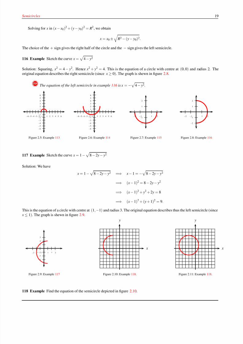
117 Example Sketch the curve x = 1 −
8 − 2 y− y2
Solution: We have
x = 1 − 8 − 2 y − y2 =⇒ x − 1 = − 8 − 2 y − y2
=⇒ ( x − 1)2 = 8 − 2 y− y2
=⇒ ( x − 1)2 + y2 + 2 y = 8
=⇒ ( x − 1)2 + ( y + 1)2 = 9.
This is the equation of a circle with centre at (1,−1) and radius 3. The original equation describes thus the left semicircle (since
x ≤ 1). The graph is shewn in figure 2.9.
1
23
−1
−2
−3
1 2 3−1−2−3
Figure 2.9: Example 117
x
y
Figure 2.10: Example 118.
x
y
Figure 2.11: Example 118.
118 Example Find the equation of the semicircle depicted in figure 2.10.
8/8/2019 Pre Calculus I
http://slidepdf.com/reader/full/pre-calculus-i 26/125
20 Chapter 2
Solution: Complete the semicircle to a full circle, as in figure 2.11. The equation of the circle is
( x + 2)2 + ( y + 1)2 = 9.
Since this is a left semi-circle, we solve for x and take the minus sign on the square root:
( x + 2)2
+ ( y + 1)2
= 9 =⇒ ( x + 2)2
= 9 − ( y + 1)2
=⇒ x + 2 = −
9 − ( y + 1)2
=⇒ x = −2 −
9 − ( y + 1)2.
The equation sought is thus
x = −2 −
9 − ( y + 1)2.
Homework
119 Problem Sketch the following curves. y =
16− x2
x = −
16− y2
x = − 12− 4 y− y2
x = −5−
12 + 4 y − y2
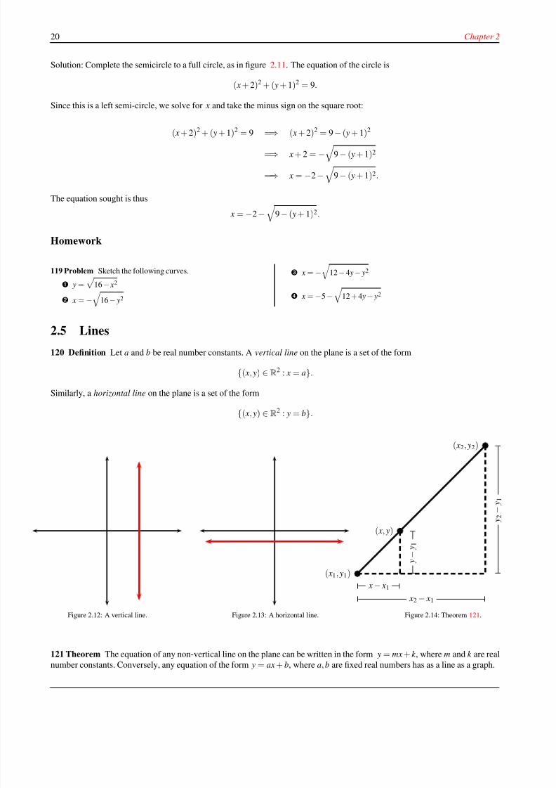
2.5 Lines
120 Definition Let a and b be real number constants. A vertical line on the plane is a set of the form
{( x, y) ∈ R2 : x = a}.
Similarly, a horizontal line on the plane is a set of the form
{( x, y) ∈ R2 : y = b}.
Figure 2.12: A vertical line. Figure 2.13: A horizontal line.
( x1, y1)
( x, y)
( x2, y2)
y 2
−
y 1
y
−
y 1
x − x1
x2 − x1
Figure 2.14: Theorem 121.
121 Theorem The equation of any non-vertical line on the plane can be written in the form y = mx + k , where m and k are real
number constants. Conversely, any equation of the form y = ax + b, where a, b are fixed real numbers has as a line as a graph.
8/8/2019 Pre Calculus I
http://slidepdf.com/reader/full/pre-calculus-i 27/125
Lines 21
Proof: If the line is parallel to the x-axis, that is, if it is horizontal, then it is of the form y= b, where b is a
constant and so we may take m = 0 and k = b. Consider now a line non-parallel to any of the axes, as in figure
2.14 , and let ( x, y) , ( x1, y1) , ( x2, y2) be three given points on the line. By similar triangles we have
y2 − y1
x2 − x1=
y − y1
x − x1,
which, upon rearrangement, gives
y =
y2 − y1
x2 − x1
x − x1
y2 − y1
x2 − x1
+ y1,
and so we may take
m =y2 − y1
x2 − x1, k = − x1
y2 − y1
x2 − x1
+ y1.
Conversely, consider real numbers x1 < x2 < x3 , and let P = ( x1, ax1 + b) , Q = ( x2, ax2 + b) , and R = ( x3, ax3 + b)be on the graph of the equation y = ax + b. We will shew that
dP, Q+ dQ, R = dP, R.
Since the points P, Q, R are arbitrary, this means that any three points on the graph of the equation y = ax + b are
collinear, and so this graph is a line. Then
dP, Q =
( x2 − x1)2 + (ax2 − ax1)2 = | x2 − x1|
1 + a2 = ( x2 − x1)
1 + a2,
dQ, R =
( x3 − x2)2 + (ax3 − ax2)2 = | x3 − x2|
1 + a2 = ( x3 − x2)
1 + a2,
dP, Q =
( x3 − x1)2 + (ax3 − ax1)2 = | x3 − x1|
1 + a2 = ( x3 − x1)
1 + a2,
from where
dP, Q + dQ, R = dP, R follows. This means that the points P, Q, and R lie on a straight line, which finishes the proof of the theorem.u
122 Definition The quantity m =y2 − y1
x2 − x1in Theorem 121 is the slope or gradient of the line joining( x1, y1) and ( x2, y2). Since
y = m(0) + k , the quantity k is the y-intercept of the line joining ( x1, y1) and ( x2, y2).
Figure 2.15: Example 123.
Figure 2.16: Example 124.
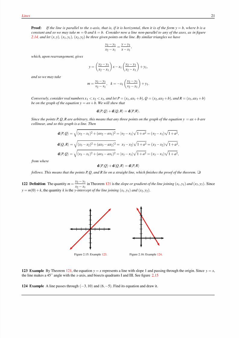
123 Example By Theorem 121, the equation y = x represents a line with slope 1 and passing through the origin. Since y = x,
the line makes a 45◦ angle with the x-axis, and bisects quadrants I and III. See figure 2.15
124 Example A line passes through (−3, 10) and (6,−5). Find its equation and draw it.
8/8/2019 Pre Calculus I
http://slidepdf.com/reader/full/pre-calculus-i 28/125
22 Chapter 2
Solution: The equation is of the form y = mx + k . We must find the slope and the y-intercept. To find m we compute the ratio
m =10− (−5)
−3 − 6= −5
3.
Thus the equation is of the form y = −5
3 x + k and we must now determine k . To do so, we substitute either point, say the first,
into y = −5
3 x + k obtaining 10 = −5
3 (−3) + k , whence k = 5. The equation sought is thus y = −5
3 x + 5. To draw the graph,
first locate the y-intercept (at (0, 5)). Since the slope is −5
3, move five units down (to (0, 0)) and three to the right (to (3, 0)).
Connect now the points (0, 5) and (3, 0). The graph appears in figure 2.16.
125 Example Three points (4, u), (1,−1) and (−3,−2) lie on the same line. Find u.
Solution: Since the points lie on the same line, any choice of pairs of points used to compute the gradient must yield the same
quantity. Thereforeu − (−1)
4 − 1=
−1 − (−2)
1 − (−3)
which simplifies to the equation
u + 13
= 14
.
Solving for u we obtain u = −1
4.
x
y
l1
l2
l3
l4
Figure 2.17: Problem 126.
0
1
2
3
0 1 2 3 4 5
Figure 2.18: Problem 127.
Homework
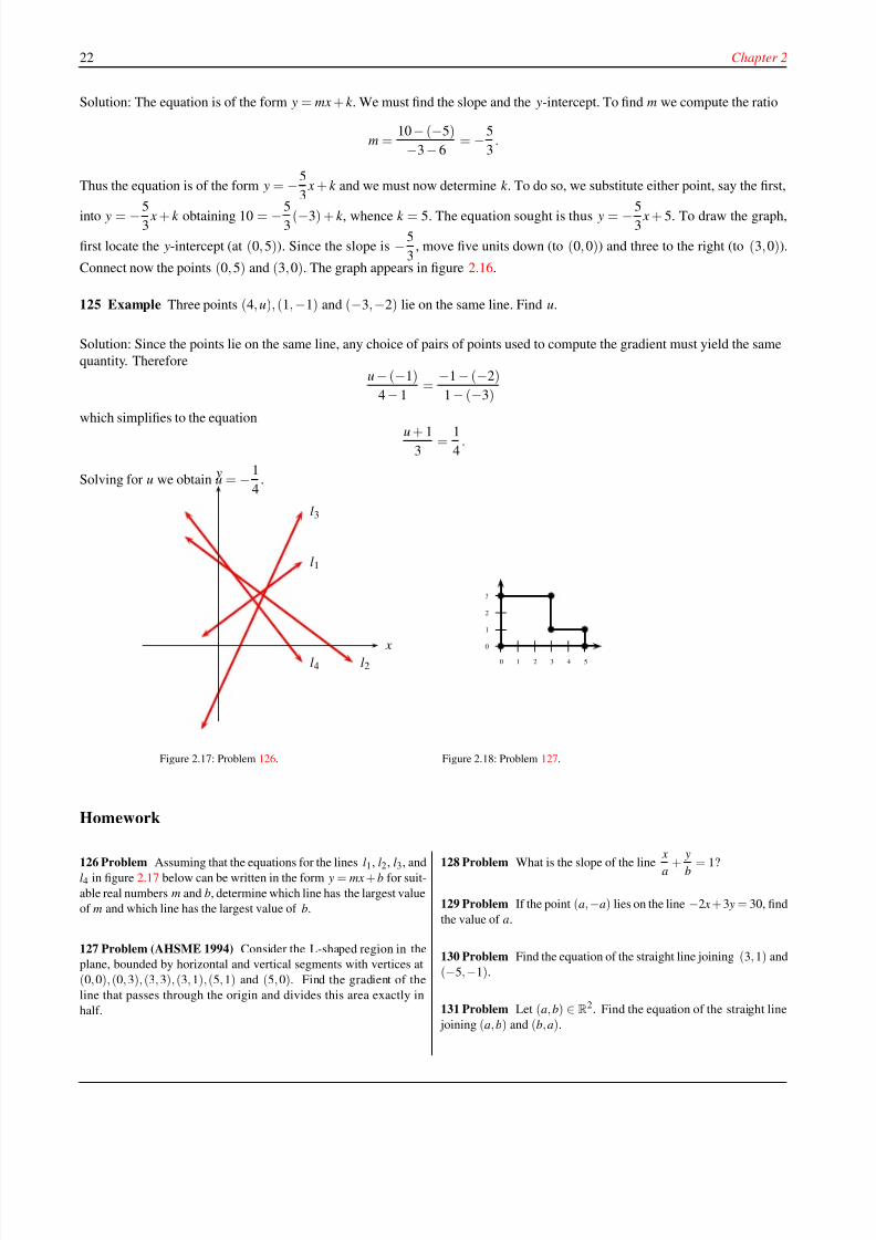
126 Problem Assuming that the equations for the lines l1, l2, l3, andl4 in figure 2.17 below can be written in the form y = mx + b for suit-
able real numbers m and b, determine which line has the largest value
of m and which line has the largest value of b.
127 Problem (AHSME 1994) Consider the L-shaped region in the
plane, bounded by horizontal and vertical segments with vertices at
(0,0), (0, 3), (3, 3), (3, 1),(5, 1) and (5, 0). Find the gradient of the
line that passes through the origin and divides this area exactly in
half.
128 Problem What is the slope of the line xa
+ yb
= 1?
129 Problem If the point (a,−a) lies on the line −2 x + 3 y = 30, find
the value of a.
130 Problem Find the equation of the straight line joining (3, 1) and
(−5,−1).
131 Problem Let (a, b) ∈ R2. Find the equation of the straight line
joining (a, b) and (b, a).
8/8/2019 Pre Calculus I
http://slidepdf.com/reader/full/pre-calculus-i 29/125
Parallel and Perpendicular Lines 23
132 Problem Find the equation of theline that passesthrough (a, a2)and (b, b2).
133 Problem The points (1, m), (2, 4) lie on a line with gradient m.
Find m.
134 Problem Consider the following regions on the plane. R1 = {( x, y) ∈ R2| y ≤ 1 − x},
R2 = {( x, y) ∈ R2| y ≥ x + 2},
R3 = {( x, y) ∈ R2| y ≤ 1 + x}.
Sketch the following regions.
R1 \ R2
R2 \ R1
R1 ∩ R2 ∩ R3
R2
\( R1
∪ R2)
135 Problem A vertical line divides the triangle with vertices
(0, 0), (1, 1) and (9,1) in the plane into two regions of equal area.
Find the equation of this vertical line.
2.6 Parallel and Perpendicular Lines
136 Definition Two lines are parallel if they have the same slope.
137 Example Find the equation of the line passing through (4, 0) and parallel to the line joining (−1, 2) and (2,−4).
Solution: First we compute the slope of the line joining (−1, 2) and (2,−4):
m =2 − (−4)
−1− 2= −2.
The line we seek is of the form y = −2 x + k . We now compute the y-intercept, using the fact that the line must pass through
(4, 0). This entails solving 0 = −2(4) + k , whence k = 8. The equation sought is finally y = −2 x + 8.
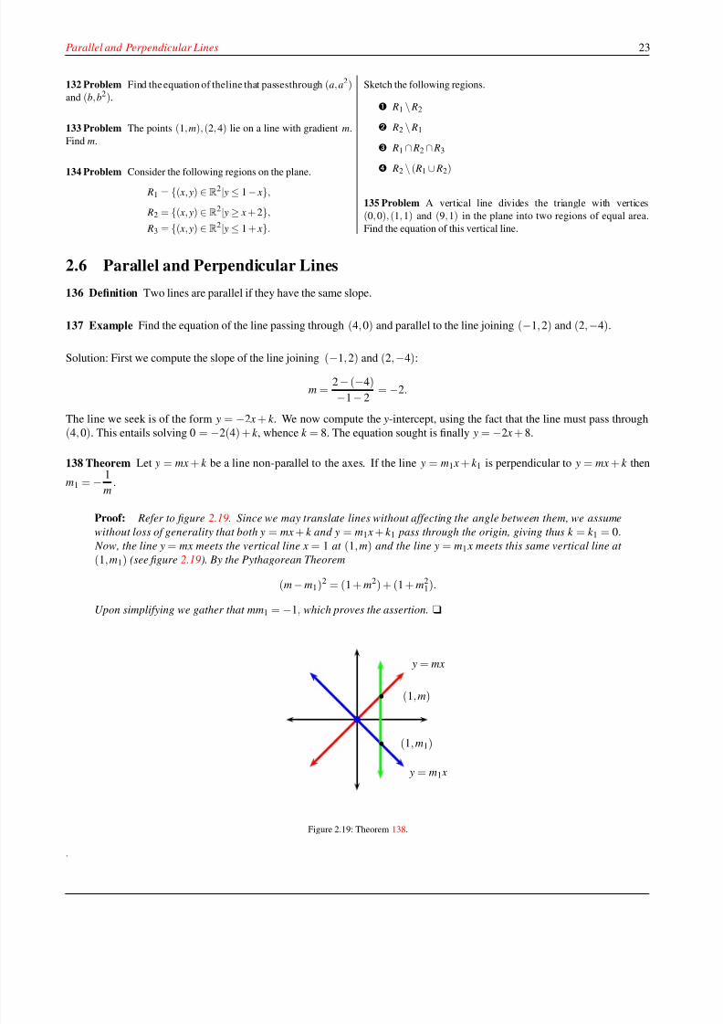
138 Theorem Let y = mx + k be a line non-parallel to the axes. If the line y = m1 x + k 1 is perpendicular to y = mx + k then
m1 = − 1
m.
Proof: Refer to figure 2.19. Since we may translate lines without affecting the angle between them, we assume
without loss of generality that both y = mx + k and y = m1 x + k 1 pass through the origin, giving thus k = k 1 = 0. Now, the line y = mx meets the vertical line x = 1 at (1, m) and the line y = m1 x meets this same vertical line at
(1, m1) (see figure 2.19). By the Pythagorean Theorem
(m − m1)2 = (1 + m2) + (1 + m21).
Upon simplifying we gather that mm1 = −1, which proves the assertion. u
y = mx
y = m1 x
•
•
(1, m)
(1, m1)
Figure 2.19: Theorem 138.
.
8/8/2019 Pre Calculus I
http://slidepdf.com/reader/full/pre-calculus-i 30/125
24 Chapter 2
139 Example Find the equation of the line passing through (4, 0) and perpendicular to the line joining (−1, 2) and (2,−4).
Solution: The slope of the line joining (−1, 2) and (2,−4) is −2. The slope of any line perpendicular to it
m1 = − 1
m=
1
2.
The equation sought has the form y = x2
+ k . We find the y-intercept by solving 0 = 42
+ k , whence k = −2. The equation of
the perpendicular line is thus y =x
2− 2.
140 Example For a given real number t , associate the straight line Lt with the equation
Lt : (4 − t ) y = (t + 2) x + 6t .
Determine t so that the point (1, 2) lies on the line Lt and find the equation of this line.
Determine t so that the Lt be parallel to the x-axis and determine the equation of the resulting line.
Determine t so that the Lt be parallel to the y-axis and determine the equation of the resulting line.
Determine t so that the Lt be parallel to the line −5 y = 3 x − 1.
Determine t so that the Lt be perpendicular to the line −5 y = 3 x − 1.
Is there a point (a, b) belonging to every line Lt regardless of the value of t ?
Solution:
If the point (1, 2) lies on the line Lt then we have
(4− t )(2) = (t + 2)(1) + 6t =⇒ t =2
3.
The line sought is thus
L2/3 : (4 − 2
3) y = (
2
3+ 2) x + 6
2
3
or y =
4
5 x +
6
5.
We need t + 2 = 0 =⇒ t = −2. In this case
(4 − (−2)) y = −12 =⇒ y = −2.
We need 4 − t = 0 =⇒ t = 4. In this case
0 = (4 + 2) x + 24 =⇒ x = −4.
The slope of Lt ist + 2
4 − t ,
and the slope of the line −5 y = 3 x − 1 is −3
5. Therefore we need
t + 2
4 − t = −3
5=⇒ −3(4 − t ) = 5(t + 2) =⇒ t = −11.
In this case we needt + 2
4 − t =
5
3=⇒ 5(4 − t ) = 3(t + 2) =⇒ t =
7
4.
8/8/2019 Pre Calculus I
http://slidepdf.com/reader/full/pre-calculus-i 31/125
Parallel and Perpendicular Lines 25
Yes. From above, the obvious candidate is (−4,−2). To verify this observe that
(4 − t )(−2) = (t + 2)(−4) + 6t ,
regardless of the value of t .
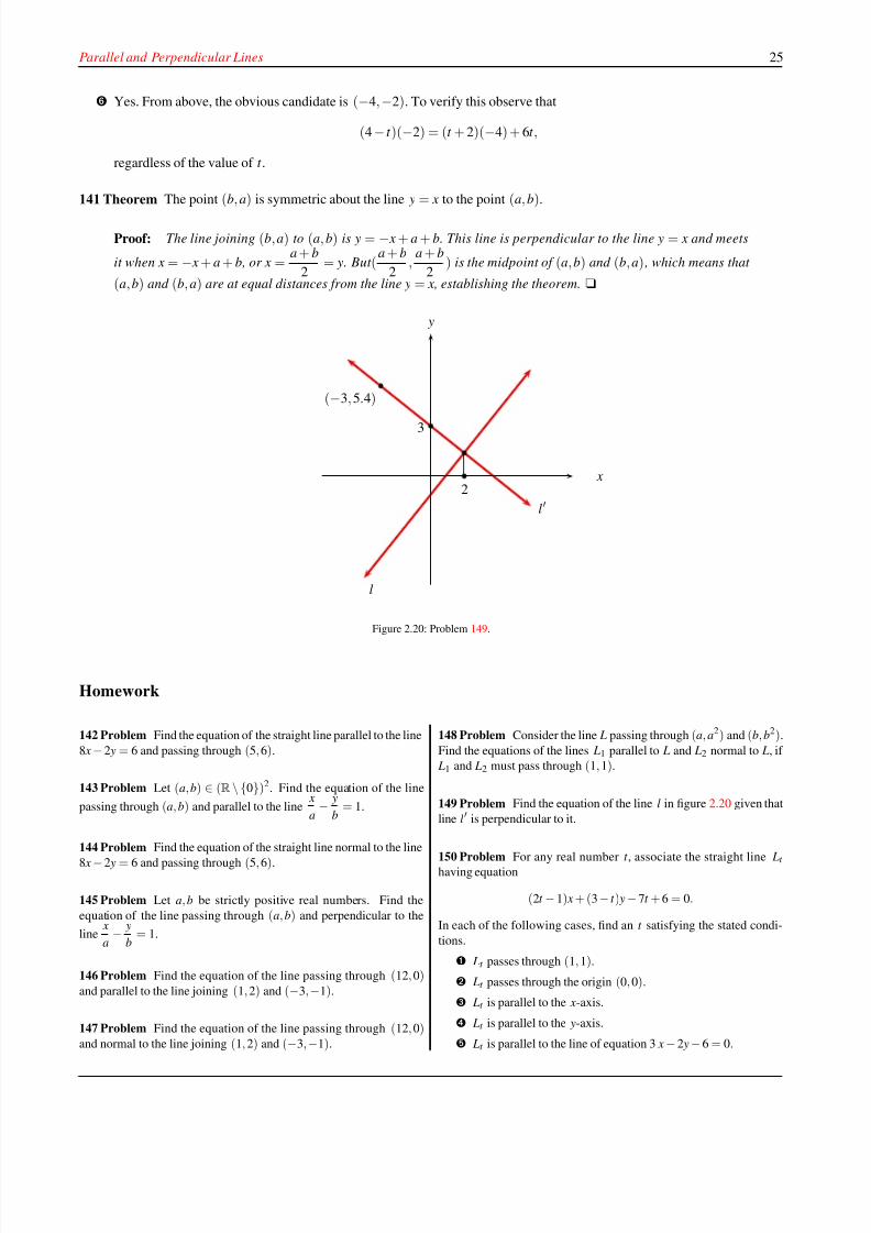
141 Theorem The point (b, a) is symmetric about the line y = x to the point (a, b).
Proof: The line joining (b, a) to (a, b) is y = − x + a + b. This line is perpendicular to the line y = x and meets
it when x = − x + a + b, or x =a + b
2= y. But (
a + b
2,
a + b
2) is the midpoint of (a, b) and (b, a) , which means that
(a, b) and (b, a) are at equal distances from the line y = x, establishing the theorem. u
3
2
(−3, 5.4)
x
y
l′
l
Figure 2.20: Problem 149.
Homework
142 Problem Find the equation of the straight line parallel to the line
8 x −2 y = 6 and passing through (5, 6).
143 Problem Let (a, b) ∈ (R \{0})2. Find the equation of the line
passing through (a, b) and parallel to the linex
a− y
b= 1.
144 Problem Find the equation of the straight line normal to the line8 x −2 y = 6 and passing through (5, 6).
145 Problem Let a, b be strictly positive real numbers. Find the
equation of the line passing through (a, b) and perpendicular to the
linex
a− y
b= 1.
146 Problem Find the equation of the line passing through (12, 0)and parallel to the line joining (1, 2) and (−3,−1).
147 Problem Find the equation of the line passing through (12, 0)and normal to the line joining (1, 2) and (−3,−1).
148 Problem Consider the line L passing through (a, a2) and (b, b2).
Find the equations of the lines L1 parallel to L and L2 normal to L, if
L1 and L2 must pass through (1, 1).
149 Problem Find the equation of the line l in figure 2.20 given that
line l′ is perpendicular to it.
150 Problem For any real number t , associate the straight line Lt
having equation
(2t −1) x + (3− t ) y −7t + 6 = 0.
In each of the following cases, find an t satisfying the stated condi-
tions.
Lt passes through (1, 1).
Lt passes through the origin (0, 0).
Lt is parallel to the x-axis.
Lt is parallel to the y-axis.
Lt is parallel to the line of equation 3 x − 2 y− 6 = 0.
8/8/2019 Pre Calculus I
http://slidepdf.com/reader/full/pre-calculus-i 32/125
8/8/2019 Pre Calculus I
http://slidepdf.com/reader/full/pre-calculus-i 33/125
8/8/2019 Pre Calculus I
http://slidepdf.com/reader/full/pre-calculus-i 34/125
28 Chapter 2
If m = 0 , then L is parallel to the x-axis and clearly
d L, P = | y0 − k |,which agrees with the theorem. Suppose now that m = 0. The line L has gradient m and any line perpendicular to
it has gradient − 1
m. The distance from P to L is the length of the line segment joining P to the intersection point
( x1, y1) of the line L1 perpendicular to L and passing through P. Now, it is easy to see that L1 has equation
L1 : y = − 1
m x + y0 +
x0
m,
and so, L and L1 intersect at
x1 =y0m + x0 − bm
1 + m2, y1 =
y0m2 + x0m + k
1 + m2.
Therefore
d L, P = d( x0, y0), ( x1, y1)
=
( x0 − x1)2 + ( y0 − y1)2
=
x0 − y0m + x0 − km
1 + m2
2+
y0 − y0m2 + x0m + k
1 + m2
2
=
( x0m2 − y0m + km)2 + ( y0 − x0m − k )2
1 + m2
=
(m2 + 1)( x0m − y0 + k )2
1 + m2
=| x0m − y0 + k |√
1 + m2,
proving the theorem. u
159 Example Find the distance between the line L : 2 x − 3 y = 1 and the point (−1, 1).
Solution: The equation of the line L can be rewritten in the form L : y =2
3 x − 1
3. Using Theorem 158, we have
d L, P =|− 2
3− 1 − 1
3|
1 + ( 23 )2
=6√
13
13.
Homework
160 Problem Find the distance from the point (1, 1) to the line
y =
− x.
161 Problem Let a ∈ R. Find the distance from the point (a, 0) to
the line L : y = ax + 1.
162 Problem Find the equation of the circle with centre at (3, 4) and
tangent to the line x− 2 y + 3 = 0.
2.9 Parabolas
163 Definition A parabola is the collection of all the points on the plane whose distance from a fixed point F (called the focus
of the parabola) is equal to the distance to a fixed line L (called the directrix of the parabola). See figure 2.26, where FD = DP.
We can draw a parabola as follows. Cut a piece of thread as long as the trunk of T-square (see figure 2.27). Tie one end to the
end of the trunk of the T-square and tie the other end to the focus, say, using a peg. Slide the crosspiece of the T-square along
the directrix, while maintaining the thread tight against the ruler with a pencil.
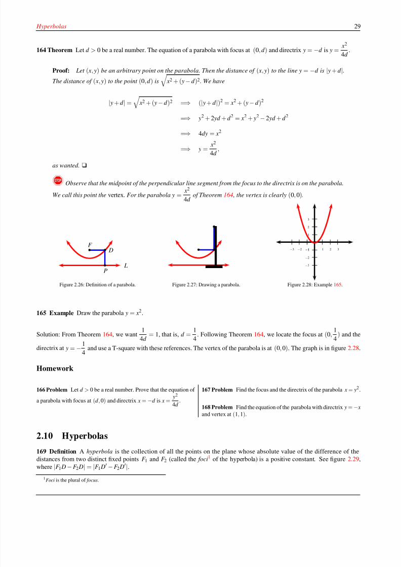
8/8/2019 Pre Calculus I
http://slidepdf.com/reader/full/pre-calculus-i 35/125
Hyperbolas 29
164 Theorem Let d > 0 be a real number. The equation of a parabola with focus at (0, d ) and directrix y = −d is y =x2
4d .
Proof: Let ( x, y) be an arbitrary point on the parabola. Then the distance of ( x, y) to the line y = −d is | y + d |.The distance of ( x, y) to the point (0, d ) is
x2 + ( y − d )2. We have
| y + d | =
x2 + ( y − d )2 =⇒ (| y + d |)2 = x2 + ( y − d )2
=⇒ y2 + 2 yd + d 2 = x2 + y2 − 2 yd + d 2
=⇒ 4dy = x2
=⇒ y =x2
4d ,
as wanted. u
! Observe that the midpoint of the perpendicular line segment from the focus to the directrix is on the parabola.
We call this point the vertex. For the parabola y =
x2
4d of Theorem 164 , the vertex is clearly (0, 0).
F D
P L
Figure 2.26: Definition of a parabola.
Figure 2.27: Drawing a parabola.
1
2
3
−1
−2
−3
1 2 3−1−2−3
Figure 2.28: Example 165.
165 Example Draw the parabola y = x2.
Solution: From Theorem 164, we want1
4d = 1, that is, d =
1
4. Following Theorem 164, we locate the focus at (0,
1
4) and the
directrix at y = −1
4and use a T-square with these references. The vertex of the parabola is at (0, 0). The graph is in figure 2.28.
Homework
166 Problem Let d > 0 be a real number. Prove that the equation of a parabola with focus at (d , 0) and directrix x = −d is x =
y2
4d .
167 Problem Find the focus and the directrix of the parabola x = y
2
.
168 Problem Find the equation of the parabola with directrix y = − x
and vertex at (1, 1).
2.10 Hyperbolas
169 Definition A hyperbola is the collection of all the points on the plane whose absolute value of the difference of the
distances from two distinct fixed points F 1 and F 2 (called the foci1 of the hyperbola) is a positive constant. See figure 2.29,
where |F 1 D − F 2 D| = |F 1 D′ − F 2 D
′|.1Foci is the plural of focus.
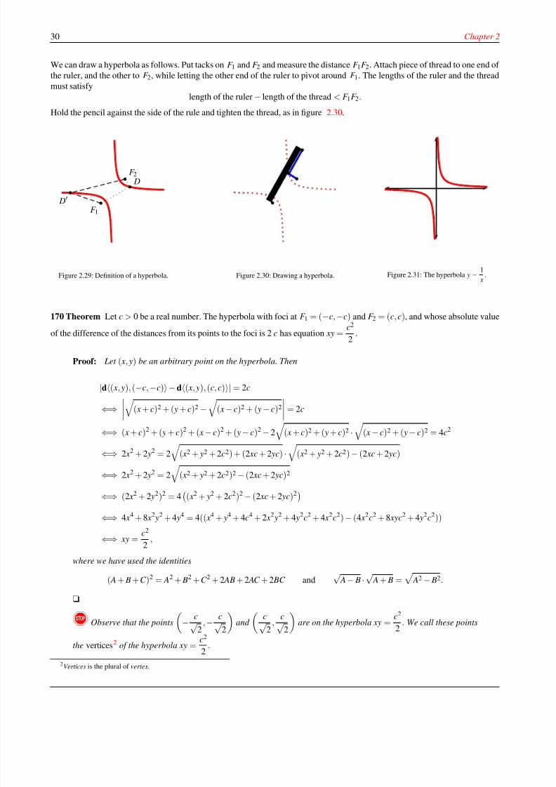
8/8/2019 Pre Calculus I
http://slidepdf.com/reader/full/pre-calculus-i 36/125
30 Chapter 2
We can draw a hyperbola as follows. Put tacks on F 1 and F 2 and measure the distance F 1F 2. Attach piece of thread to one end of
the ruler, and the other to F 2, while letting the other end of the ruler to pivot around F 1. The lengths of the ruler and the thread
must satisfy
length of the ruler − length of the thread < F 1F 2.
Hold the pencil against the side of the rule and tighten the thread, as in figure 2.30.
F 1
F 2 D
D′
Figure 2.29: Definition of a hyperbola.
Figure 2.30: Drawing a hyperbola. Figure 2.31: The hyperbola y = 1 x
.
170 Theorem Let c > 0 be a real number. The hyperbola with foci at F 1 = (−c,−c) and F 2 = (c, c), and whose absolute value
of the difference of the distances from its points to the foci is 2c has equation xy =c2
2.
Proof: Let ( x, y) be an arbitrary point on the hyperbola. Then
|d( x, y), (−c,−c)− d( x, y), (c, c)| = 2c
⇐⇒ ( x + c)2 + ( y + c)2 − ( x − c)2 + ( y − c)2 = 2c
⇐⇒ ( x + c)2 + ( y + c)2 + ( x − c)2 + ( y − c)2 − 2
( x + c)2 + ( y + c)2 ·
( x − c)2 + ( y− c)2 = 4c2
⇐⇒ 2 x2 + 2 y2 = 2
( x2 + y2 + 2c2) + (2 xc + 2 yc) ·
( x2 + y2 + 2c2)− (2 xc + 2 yc)
⇐⇒ 2 x2 + 2 y2 = 2
( x2 + y2 + 2c2)2 − (2 xc + 2 yc)2
⇐⇒ (2 x2 + 2 y2)2 = 4
( x2 + y2 + 2c2)2 − (2 xc + 2 yc)2
⇐⇒ 4 x4 + 8 x2 y2 + 4 y4 = 4(( x4 + y4 + 4c4 + 2 x2 y2 + 4 y2c2 + 4 x2c2) − (4 x2c2 + 8 xyc2 + 4 y2c2))
⇐⇒xy =
c2
2,
where we have used the identities
( A + B +C )2 = A2 + B2 +C 2 + 2 AB + 2 AC + 2 BC and√
A − B ·√ A + B =
A2 − B2.
u
! Observe that the points
− c√
2,− c√
2
and
c√
2,
c√2
are on the hyperbola xy =
c2
2. We call these points
the vertices2 of the hyperbola xy =c2
2.
2Vertices is the plural of vertex.
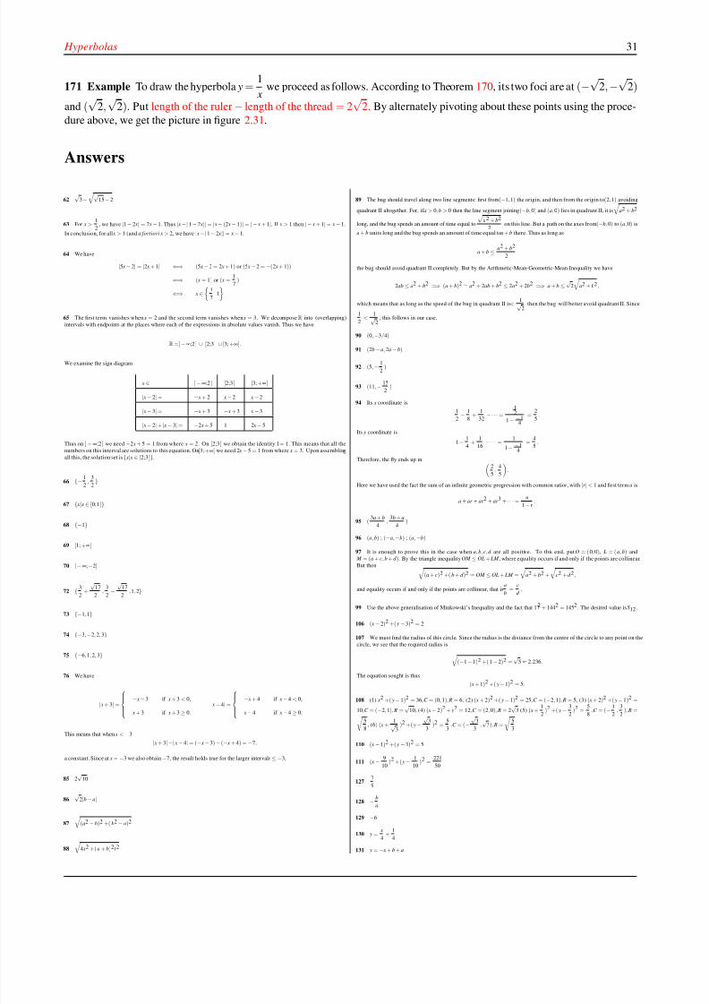
8/8/2019 Pre Calculus I
http://slidepdf.com/reader/full/pre-calculus-i 37/125
Hyperbolas 31
171 Example To draw the hyperbola y =1
xwe proceed as follows. According to Theorem 170, its two foci are at (−
√2,−
√2)
and (√
2,√
2). Put length of the ruler − length of the thread = 2√
2. By alternately pivoting about these points using the proce-
dure above, we get the picture in figure 2.31.
Answers
62√
3− √
15 −2
63 For x >1
2, we have |1− 2 x| = 2 x − 1. Thus | x −|1 − 2 x|| = | x − (2 x− 1)| = |− x + 1|. If x > 1 then |− x + 1| = x − 1.
In conclusion, for all x > 1 (and a fortiori x > 2, we have | x −|1− 2 x|| = x− 1.
64 We have
|5 x− 2| = |2 x + 1| ⇐⇒ (5 x− 2 = 2 x + 1) or (5 x − 2 = −(2 x + 1))
⇐⇒ ( x = 1) or ( x =1
7)
⇐⇒ x ∈
1
7, 1
65 The first term vanishes when x = 2 and the second term vanishes when x = 3. We decompose R into (overlapping)
intervals with endpoints at the places where each of the expressions in absolute values vanish. Thus we have
R=]−∞;2 ]
∪[2;3 ]
∪[3; +∞[.
We examine the sign diagram
x ∈ ]−∞;2 ] [2;3 ] [3; +∞[
| x− 2| = − x + 2 x− 2 x −2
| x− 3| = − x + 3 − x + 3 x −3
| x− 2| + | x − 3| = −2 x + 5 1 2 x − 5
Thus on ] −∞;2 ] we need −2 x + 5 = 1 from where x = 2. On [2;3 ] we obtain the identity 1 = 1. This means that all the
numbers on this interval are solutions to this equation. On [3; +∞[ we need 2 x −5 = 1 from where x = 3. Upon assembling
all this, the solution set is { x| x ∈ [2;3 ]}.
66 {− 1
2,
3
2}
67 { x| x ∈ [0;1 ]}
68 {−1}
69 [1; +∞[
70 ]−∞;−2]
72 { 3
2+
√17
2,
3
2−
√17
2, 1, 2}
73 {−1, 1}
74 {−3,−2, 2, 3}
75 {−6, 1, 2, 3}
76 We have
| x + 3| =
− x −3 if x + 3 < 0,
x + 3 if x + 3 ≥ 0.
| x −4| =
− x + 4 if x −4 < 0,
x −4 if x −4 ≥ 0.
This means that when x < −3
| x + 3|−| x− 4| = (− x− 3) −(− x + 4) = −7,
a constant. Since at x = −3 we also obtain −7, the result holds true for the larger interval x ≤ −3.
85 2√
10
86√
2|b −a|
87
(a2 − b)2 +( b2 − a)2
88
4 x2 +( a + b)2t 2
89 The bug should travel along two line segments: first from (−1, 1) the origin, and then from the origin to (2, 1) avoiding
quadrant II altogether. For, if a > 0, b > 0 then the line segment joining (−b, 0) and (a, 0) lies in quadrant II, it is
a2 + b2
long, and the bug spends an amount of time equal to
a2 + b2
2on this line. But a path on the axes from (−b, 0) to (a, 0) is
a + b units long and the bug spends an amount of time equal to a + b there. Thus as long as
a + b ≤ a2 + b2
2
the bug should avoid quadrant II completely. But by the Arithmetic-Mean-Geometric-Mean Inequality we have
2ab ≤ a2 + b2 =⇒ (a + b)2 = a2 + 2ab + b2 ≤ 2a2 + 2b2 =⇒ a + b ≤√
2
a2 + b2 ,
which means that as long as the speed of the bug in quadrant II is <1√
2then the bug will better avoid quadrant II. Since
1
2<
1√2
, this follows in our case.
90 (0,−3/4)
91 (2b −a, 2a − b)
92 (5,− 1
2)
93 (11,− 15
2)
94 Its x coordinate is
1
2− 1
8+
1
32−··· =
12
1− −14
=2
5.
Its y coordinate is
1− 1
4+
1
16−··· =
1
1− −14
=4
5.
Therefore, the fly ends up in 2
5,
4
5
.
Here we have used the fact the sum of an infinite geometric progression with common ratio r , with |r | < 1 and first term a is
a + ar + ar 2 + ar 3 + ·· · =a
1 −r .
95 (3a + b
4 ,3b + a
4 )
96 (a, b) ; (−a,−b) ; (a,−b)
97 It is enough to prove this in the case when a, b, c, d are all positive. To this end, put O = ( 0, 0), L = ( a, b) and M = (a + c, b + d ). By the triangle inequality OM ≤ OL + LM , where equality occurs if and only if the points are collinear.
But then (a + c)2 +( b + d )2 = OM ≤ OL + LM =
a2 + b2 +
c2 + d 2,
and equality occurs if and only if the points are collinear, that isa
b=
c
d .
99 Use the above generalisation of Minkowski’s Inequality and the fact that 17 2 + 1442 = 1452 . The desired value is S12 .
106 ( x − 2)2 +( y −3)2 = 2
107 We must find the radius of this circle. Since the radius is the distance from the centre of the circle to any point on the
circle, we see that the required radius is
(−1 −1)2 +( 1− 2)2 =
√5 ≈ 2.236.
The equation sought is thus
( x + 1)2 +( y− 1)2 = 5.
108 (1) x2 +( y− 1)2 = 36,C = (0, 1), R = 6. (2) ( x + 2)2 +( y − 1)2 = 25,C = (−2, 1), R = 5, (3) ( x + 2)2 +( y− 1)2 =
10,C = (−2, 1), R =√
10, (4) ( x − 2)2 + y2 = 12,C = (2, 0), R = 2√
3 (5) ( x +1
2)2 +( y − 3
2)2 =
5
8,C = (− 1
2,
3
2), R =
5
8, (6) ( x +
1√3
)2 +( y−√
3
3)2 =
5
3,C = (−
√3
3,√
3), R =
5
3
110 ( x − 1)2 +( y −3)2 = 5
111 ( x − 9
10)2 +( y− 1
10)2 =
221
50
1277
9
128 − b
a
129 −6
130 y =x
4+
1
4
131 y = − x + b + a
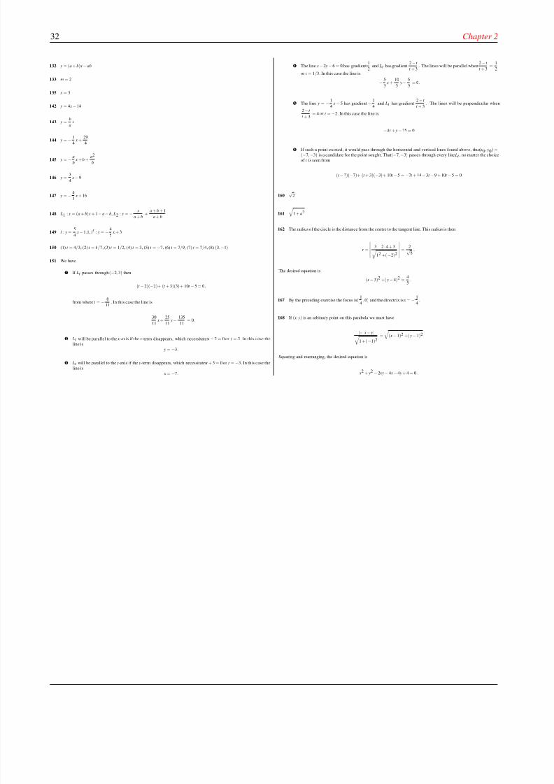
8/8/2019 Pre Calculus I
http://slidepdf.com/reader/full/pre-calculus-i 38/125
32 Chapter 2
132 y = (a + b) x − ab
133 m = 2
135 x = 3
142 y = 4 x− 14
143 y =b
a x
144 y = − 1
4x +
29
4
145 y = − a
b x + b +
a2
b
146 y =3
4x − 9
147 y = − 4
3x + 16
148 L1 : y = (a + b) x + 1− a− b, L2 : y = − x
a + b+
a + b + 1
a + b
149 l : y =5
4x −1.1, l′ : y = − 4
5x + 3
150 (1) t = 4/3, (2) t = 6/7, (3) t = 1/2, (4) t = 3, (5) t = −7, (6) t = 7/9, (7) t = 7/4, (8) (3,−1)
151 We have
If Lt passes through (−2, 3) then
(t − 2)(−2)+ (t + 3)(3)+ 10t − 5 = 0,
from where t = − 8
11. In this case the line is
− 30
11x +
25
11y − 135
11= 0.
Lt will be parallel to the x-axis if the x-term disappears, which necessitates t − 2 = 0 or t = 2. In this case the
line is y = −3.
Lt will be parallel to the y-axis if the y-term disappears, which necessitates t + 3 = 0 or t = −3. In this case the
line is
x = −7.
The line x − 2 y − 6 = 0 has gradient1
2and Lt has gradient
2− t
t + 3. The lines will be parallel when
2 − t
t + 3=
1
2or t = 1/3. In this case the line is
− 5
3x +
10
3y − 5
3= 0.
The line y = − 1
4x − 5 has gradient − 1
4and Lt has gradient
2 − t
t + 3. The lines will be perpendicular when
2 − t
t + 3= 4 or t = −2. In this case the line is
−4 x + y
−25 = 0.
If such a point existed, it would pass through the horizontal and vertical lines found above, thus ( x0 , y0) =(−7,−3) is a candidate for the point sought. That (−7,−3) passes through every line Lt , no matter the choice
of t is seen from
(t − 2)(−7)+ (t + 3)(−3)+ 10t −5 = −7t + 14 −3t − 9 + 10t −5 = 0.
160√
2
161
1 + a2
162 The radius of the circle is the distance from the centre to the tangent line. This radius is then
r =
3 − 2 ·4 + 3 12 +(−2)2
=2√
5.
The desired equation is
( x −3)2 +( y− 4)2 =4
5.
167 By the preceding exercise the focus is (1
4, 0) and the directrix is x = − 1
4.
168 If ( x, y) is an arbitrary point on this parabola we must have
|− x− y| 1 +(−1)2
=
( x −1)2 +( y− 1)2
Squaring and rearranging, the desired equation is
x2 + y2 − 2 xy − 4 x −4 y + 4 = 0.
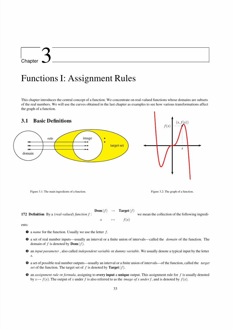
8/8/2019 Pre Calculus I
http://slidepdf.com/reader/full/pre-calculus-i 39/125
Chapter
3Functions I: Assignment Rules
This chapter introduces the central concept of a function. We concentrate on real-valued functions whose domains are subsets
of the real numbers. We will use the curves obtained in the last chapter as examples to see how various transformations affect
the graph of a function.
3.1 Basic Definitions
domain
imagerule
target set
Figure 3.1: The main ingredients of a function.
( x, f ( x)) f ( x)
x
Figure 3.2: The graph of a function.
172 Definition By a (real-valued) function f :Dom( f ) → Target ( f )
x → f ( x)
we mean the collection of the following ingredi-
ents:
a name for the function. Usually we use the letter f .
a set of real number inputs—usually an interval or a finite union of intervals—called the domain of the function. The
domain of f is denoted by Dom( f ).
an input parameter , also called independent variable or dummy variable. We usually denote a typical input by the letter
x.
a set of possible real number outputs—usually an interval or a finite union of intervals—of the function, called the target
set of the function. The target set of f is denoted by Target ( f ).
an assignment rule or formula, assigning to every input a unique output. This assignment rule for f is usually denoted
by x → f ( x). The output of x under f is also referred to as the image of x under f , and is denoted by f ( x).
33
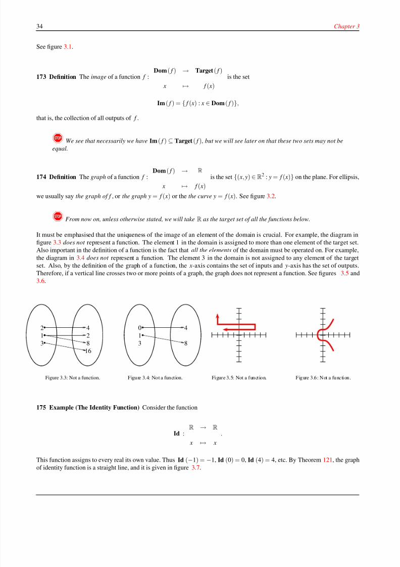
8/8/2019 Pre Calculus I
http://slidepdf.com/reader/full/pre-calculus-i 40/125
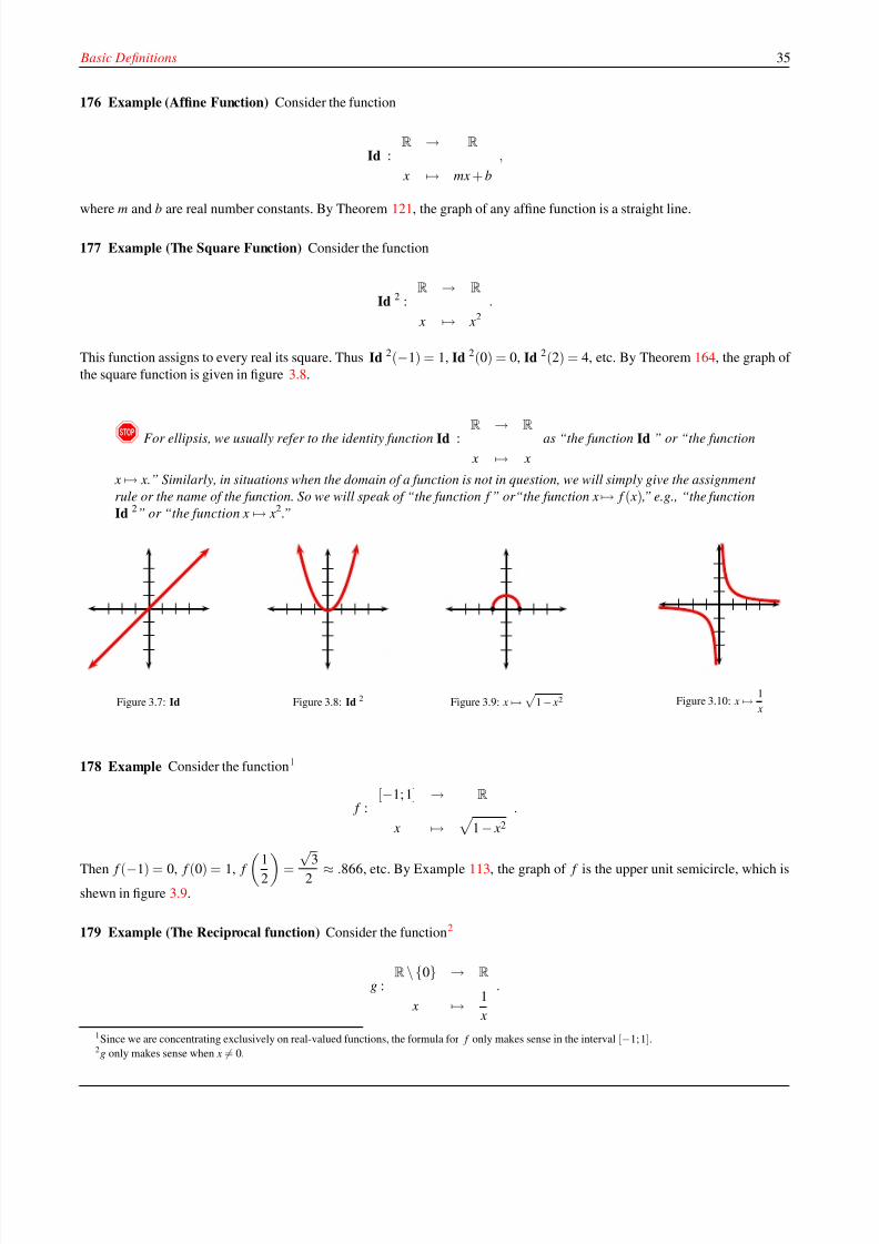
8/8/2019 Pre Calculus I
http://slidepdf.com/reader/full/pre-calculus-i 41/125
Basic Definitions 35
176 Example (Affine Function) Consider the function
Id :R → R
x → mx + b
,
where m and b are real number constants. By Theorem 121, the graph of any affine function is a straight line.
177 Example (The Square Function) Consider the function
Id 2 :R → R
x → x2
.
This function assigns to every real its square. Thus Id 2(−1) = 1, Id 2(0) = 0, Id 2(2) = 4, etc. By Theorem 164, the graph of
the square function is given in figure 3.8.
! For ellipsis, we usually refer to the identity functionId : R → R
x → x
as “the function Id ” or “the function
x → x.” Similarly, in situations when the domain of a function is not in question, we will simply give the assignment
rule or the name of the function. So we will speak of “the function f ” or“the function x→ f ( x) ,” e.g., “the function
Id 2” or “the function x → x2.”
Figure 3.7: Id Figure 3.8: Id 2
Figure 3.9: x →
1 − x2 Figure 3.10: x → 1
x
178 Example Consider the function1
f :[−1; 1] → R
x →
1 − x2
.
Then f (−1) = 0, f (0) = 1, f 1
2
= √3
2≈ .866, etc. By Example 113, the graph of f is the upper unit semicircle, which is
shewn in figure 3.9.
179 Example (The Reciprocal function) Consider the function2
g :R\{0} → R
x → 1
x
.
1Since we are concentrating exclusively on real-valued functions, the formula for f only makes sense in the interval [−1;1].2g only makes sense when x = 0.
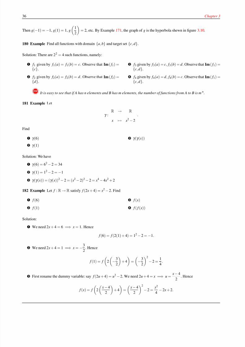
8/8/2019 Pre Calculus I
http://slidepdf.com/reader/full/pre-calculus-i 42/125
36 Chapter 3
Then g(−1) = −1, g(1) = 1, g
1
2
= 2, etc. By Example 171, the graph of g is the hyperbola shewn in figure 3.10.
180 Example Find all functions with domain {a, b} and target set {c, d }.
Solution: There are 22 = 4 such functions, namely:
f 1 given by f 1(a) = f 1(b) = c. Observe that Im ( f 1) ={c}.
f 2 given by f 2(a) = f 2(b) = d . Observe that Im ( f 2) ={d }.
f 3 given by f 3(a) = c, f 3(b) = d . Observe that Im ( f 1) ={c, d }.
f 4 given by f 4(a) = d , f 4(b) = c. Observe that Im ( f 1) ={c, d }.
! It is easy to see that if A has n elements and B has m elements, the number of functions from A to B is mn.
181 Example Let
γ :R → R
x → x2 − 2
.
Find
γ (6)
γ (1)
γ (γ ( x))
Solution: We have
γ (6) = 62 − 2 = 34
γ (1) = 12 − 2 = −1
γ (γ ( x)) = (γ ( x))2 − 2 = ( x2 − 2)2 − 2 = x4 − 4 x2 + 2
182 Example Let f : R→R satisfy f (2 x + 4) = x2 − 2. Find
f (6)
f (1)
f ( x)
f ( f ( x))
Solution:
We need 2 x + 4 = 6 =⇒ x = 1. Hence
f (6) = f (2(1) + 4) = 12
−2 =
−1.
We need 2 x + 4 = 1 =⇒ x = −3
2. Hence
f (1) = f
2
−3
2
+ 4
=
−3
2
2
− 2 =1
4.
First rename the dummy variable: say f (2u + 4) = u2 − 2. We need 2u + 4 = x =⇒ u =x − 4
2. Hence
f ( x) = f
2
x − 4
2
+ 4
=
x − 4
2
2
− 2 =x2
4− 2 x + 2.
8/8/2019 Pre Calculus I
http://slidepdf.com/reader/full/pre-calculus-i 43/125
Basic Definitions 37
Using the above part,
f ( f ( x)) =( f ( x))2
4− 2 f ( x) + 2
=
x2
4− 2 x + 2
2
4− 2
x2
4− 2 x + 2
+ 2
= x4
64− x
3
4+ 3 x
2
4+ 2 x − 1
183 Example f : R→ R is a function satisfying f (3) = 2 and f ( x + 3) = f (3) f ( x). Find f (−3).
Solution: Since we are interested in f (−3), we first put x = −3 in the relation, obtaining
f (0) = f (3) f (−3).
Thus we must also know f (0) in order to find f (−3). Letting x = 0 in the relation,
f (3) = f (3) f (−3) =⇒ f (−3) = 1.
Notice that the fact that f (3) = 2 is irrelevant, we only need f (3) = 0.
184 Example (Cauchy’s Functional Equation) Suppose f satisfies f ( x + y) = f ( x) + f ( y). Prove that ∃c ∈ R such that
f ( x) = cx, ∀ x ∈Q.
Solution: Letting y = 0 we obtain f ( x) = f ( x) + f (0), and so f (0) = 0. If k is a positive integer we obtain
f (kx) = f ( x + (k − 1) x)
= f ( x) + f ((k − 1) x)
= f ( x) + f ( x) + f ((k − 2) x) = 2 f ( x) + f ((k − 2) x)
= 2 f ( x) + f ( x) + f ((k − 3) x) = 3 f ( x) + f ((k − 3) x)
...
= · · · = k f ( x) + f (0) = k f ( x).
Letting y = − x we obtain 0 = f (0) = f ( x) + f (− x) and so f (− x) = − f ( x). Hence f (nx) = n f ( x) for n ∈ Z. Let x ∈Q, which
means that x =s
t for integers s, t with t = 0. This means that tx = s · 1 and so f (tx) = f (s · 1) and by what was just proved
for integers, t f ( x) = s f (1). Hence f ( x) =s
t f (1) = x f (1). Since f (1) is a constant, we may put c = f (1). Thus f ( x) = cx for
rational numbers x.
Homework
185 Problem Draw thegraph of thefunction f :R → R
x → |2 x −1|and find f (−1), f (0), f (1).
186 Problem Find all functions from {0, 1, 2} to {−1, 1}.
187 Problem Find all functions from {−1, 1} to {0,1, 2} .
188 Problem Let f : Dom ( f ) → R be a function. f is said to
have a fixed point at t ∈ Dom ( f ) if f (t ) = t . Let s : [0; +∞[→ R,
s( x) = x5 − 2 x3 + 2 x. Find all fixed points of s.
189 Problem Let f :R→R, x → x2 − x. Find
f ( x + h) − f ( x −h)
h.
8/8/2019 Pre Calculus I
http://slidepdf.com/reader/full/pre-calculus-i 44/125
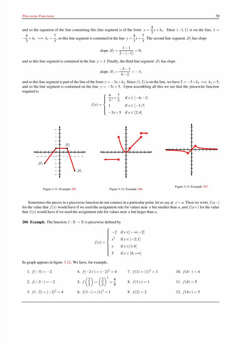
8/8/2019 Pre Calculus I
http://slidepdf.com/reader/full/pre-calculus-i 45/125
Piecewise Functions 39
and so the equation of the line containing this line segment is of the form y =4
3 x + k 1. Since (−1, 1) is on the line, 1 =
−4
3+ k 1 =⇒ k 1 =
7
3, so this line segment is contained in the line y =
4
3 x +
7
3. The second line segment L 2 has slope
slope L 2 =1 − 1
2 − (−1)= 0,
and so this line segment is contained in the line y = 1. Finally, the third line segment L 3 has slope
slope L 3 =−5 − 1
4 − 2= −3,
and so this line segment is part of the line of the form y = −3 x + k 2. Since (1, 2) is on the line, we have 2 = −3+ k 2 =⇒ k 2 = 5,
and so the line segment is contained on the line y = −3 x + 5. Upon assembling all this we see that the piecewise function
required is
f ( x) =
4
3 x +
7
3if x ∈ [−4;−1]
1 if x ∈ [−1; 2]
−3 x + 5 if x ∈ [2; 4]
1
2
3
4
5
6
−1
−2
−3
−4
−5
−6
1 2 3 4 5 6−1−2−3−4−5−6
L 1
L 2
L 3
Figure 3.11: Example 205.
Figure 3.12: Example 206.
Figure 3.13: Example 207.
Sometimes the pieces in a piecewise function do not connect at a particular point, let us say at x = a. Then we write f (a−)for the value that f ( x) would have if we used the assignment rule for values near a but smaller than a, and f (a+) for the value
that f ( x) would have if we used the assignment rule for values near a but larger than a.
206 Example The function f : R→ R is piecewise defined by
f ( x) =
−2 if x ∈]−∞;−2[
x2
if x ∈ [−2; 1] x if x ∈]1; 4[
5 if x ∈ [4; +∞[
Its graph appears in figure 3.12. We have, for example,
1. f (−3) = −2
2. f (−2−) = −2
3. f (−2) = (−2)2 = 4
4. f (−2+) = (−2)2 = 4
5. f
2
3
=
2
3
2
=4
9
6. f (1−) = (1)2 = 1
7. f (1) = (1)2 = 1
8. f (1+) = 1
9. f (2) = 2
10. f (4−) = 4
11. f (4) = 5
12. f (4+) = 5
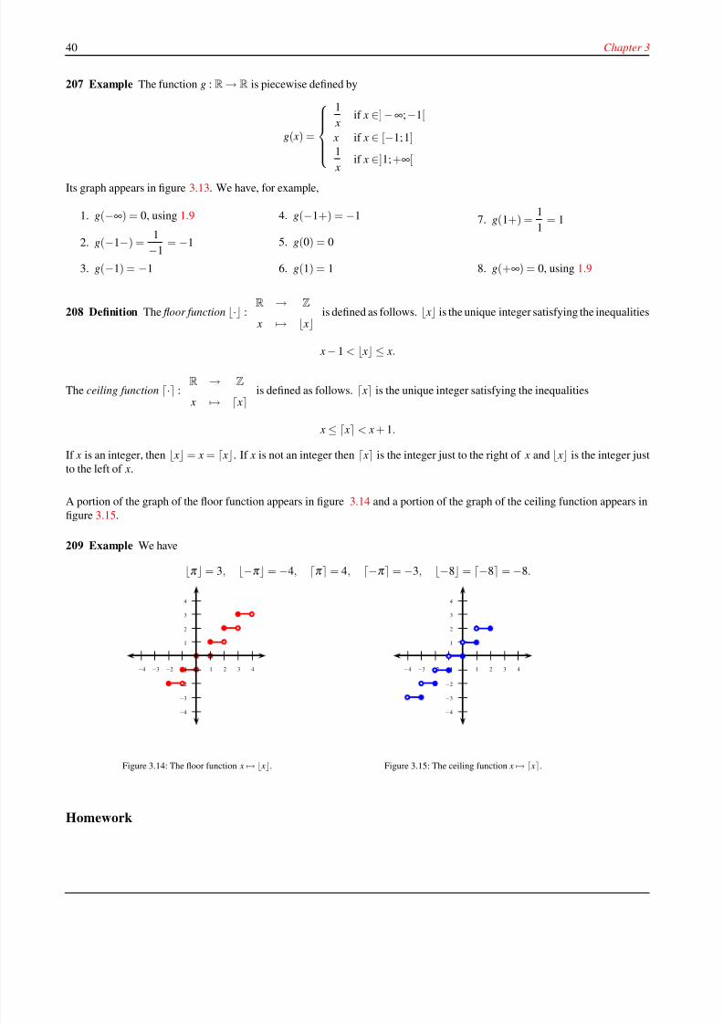
8/8/2019 Pre Calculus I
http://slidepdf.com/reader/full/pre-calculus-i 46/125
40 Chapter 3
207 Example The function g : R→ R is piecewise defined by
g( x) =
1
xif x ∈] −∞;−1[
x if x ∈ [−1; 1]1
xif x ∈]1; +∞[
Its graph appears in figure 3.13. We have, for example,
1. g(−∞) = 0, using 1.9
2. g(−1−) =1
−1= −1
3. g(−1) = −1
4. g(−1+) = −1
5. g(0) = 0
6. g(1) = 1
7. g(1+) =1
1= 1
8. g(+∞) = 0, using 1.9
208 Definition The floor function ⌊·⌋ :R → Z
x → ⌊ x⌋is defined as follows. ⌊ x⌋ is the unique integer satisfying the inequalities
x − 1 < ⌊ x⌋ ≤ x.
The ceiling function ⌈·⌉ :R → Z
x → ⌈ x⌉is defined as follows. ⌈ x⌉ is the unique integer satisfying the inequalities
x ≤ ⌈ x⌉ < x + 1.
If x is an integer, then ⌊ x⌋ = x = ⌈ x⌋. If x is not an integer then ⌈ x⌉ is the integer just to the right of x and ⌊ x⌋ is the integer just
to the left of x.
A portion of the graph of the floor function appears in figure 3.14 and a portion of the graph of the ceiling function appears in
figure 3.15.
209 Example We have
⌊π ⌋ = 3, ⌊−π ⌋ = −4, ⌈π ⌉ = 4, ⌈−π ⌉ = −3, ⌊−8⌋ = ⌈−8⌉ = −8.
1
2
3
4
−1
−2
−3
−4
1 2 3 4−1−2−3−4
Figure 3.14: The floor function x → ⌊ x⌋.
1
2
3
4
−1
−2
−3
−4
1 2 3 4−1−2−3−4
Figure 3.15: The ceiling function x → ⌈ x⌉.
Homework
8/8/2019 Pre Calculus I
http://slidepdf.com/reader/full/pre-calculus-i 47/125
Translations 41
210 Problem Write f :R→R, f ( x) = | x−1|+ | x+2| as a piecewise
function. Graph this function.
211 Problem Write f :R→R, f ( x) = x| x| as a piecewise function.
212 Problem Write f :R
→R, f ( x) = x+
| x
|as a piecewise function
and draw its graph.
213 Problem Graph x → ⌊2 x⌋.
214 Problem Graph x → ⌊ x2⌋.
215 Problem Let g :R→R be piecewise defined by
g( x) =
1
xif x ∈] −∞;−1[
| x| if x ∈ [−1; 1]
1 + 2 x if x ∈]1; +∞[
Graph it and determine
1. g(−∞)
2. g(−1−)
3. g(−1)
4. g(−1+)
5. g(0)
6. g(1−)
7. g(1)
8. g(1+)
9. g(+∞)
216 Problem Solve the equation ⌊ x
5⌋ = 10.
3.3 Translations
In this section we study how several rigid transformations affect both the graph of a function and its assignment rule.
217 Theorem Let f be a function and let v and h be real numbers. If ( x0, y0) is on the graph of f , then ( x0, y0 + v) is on the
graph of g, where g( x) = f ( x) +v, and if ( x1, y1) is on the graph of f , then ( x1 −h, y1) is on the graph of j, where j( x) = f ( x +h).
Proof: Let Γ f ,Γ g,Γ j denote the graphs of f , g, j respectively.
( x0, y0) ∈ Γ f ⇐⇒ y0 = f ( x0) ⇐⇒ y0 + v = f ( x0) + v ⇐⇒ y0 + v = g( x0) ⇐⇒ ( x0, y0 + v) ∈ Γ g.
Similarly,
( x1, y1) ∈ Γ f ⇐⇒ y1 = f ( x1) ⇐⇒ y1 = f ( x1 − h + h) ⇐⇒ y1 = j( x1 − h) ⇐⇒ ( x1 − h, y1) ∈ Γ j.
u
218 Definition Let f be a function and let v and h be real numbers. We say that the curve y = f ( x) + v is a vertical translation
of the curve y = f ( x). If v > 0 the translation is v up, and if v < 0, it is v units down. Similarly, we say that the curve y = f ( x + h)is a horizontal translation of the curve y = f ( x). If h > 0, the translation is h units left, and if h < 0, then the translation is h
units right.

8/8/2019 Pre Calculus I
http://slidepdf.com/reader/full/pre-calculus-i 48/125
42 Chapter 3
219 Example If f ( x) = x2, then figures 3.16, 3.17 and 3.18 shew vertical translations 3 units up and 3 units down, respectively.
Figures 3.19, 3.20, and 3.21, respectively shew a horizontal translation 3 units right, 3 units left, and a simultaneous translation
3 units left and down. The corresponding assignment rules are
a( x) = f ( x) + 3 = x2 + 3, b( x) = f ( x) − 3 = x2 − 3; c( x) = f ( x + 3) = ( x − 3)2; d ( x) = ( x + 3)2; g( x) = ( x + 3)2 − 3
Figure 3.16: y = f ( x) = x2
Figure 3.17: y =a( x) = x2 + 3
Figure 3.18: y =b( x) = x2
−3
Figure 3.19: y =c( x) = ( x
−3)2
Figure 3.20: y =d ( x) = ( x + 3)2
Figure 3.21: y =g( x) = ( x + 3)2 −3
220 Example If g( x) = x (figure 3.22), then figures , 3.23 and 3.24 shew vertical translations 3 units up and 3 units down,
respectively. Notice than in this case g( x + t ) = x + t = g( x) + t , so a vertical translation by t units has exactly the same graph
as a horizontal translation t units.
Figure 3.22: y = g( x) = x Figure 3.23: y = g( x)+ 3 = x + 3 Figure 3.24: y = g( x)− 3 = x −3
221 Definition Given a function f we write f (−∞) for the value that f may eventually approach for large (in absolute value)
and negative inputs and f (+∞) for the value that f may eventually approach for large (in absolute value) and positive input.The line y = b is a (horizontal) asymptote for the function f if either
f (−∞) = b or f (+∞) = b.
222 Definition Let k > 0 be an integer. A function f has a pole of order k at the point x = a if ( x−a)k −1 f ( x) → ±∞ as x → a,
but ( x − a)k f ( x) as x → a is finite. Some authors prefer to use the term vertical asymptote, rather than pole.
223 Example Since x f ( x) = 1, f (0−) = −∞, f (0+) = +∞ for f :R\{0} → R
x → 1
x
, f has a pole of order 1 at x = 0.
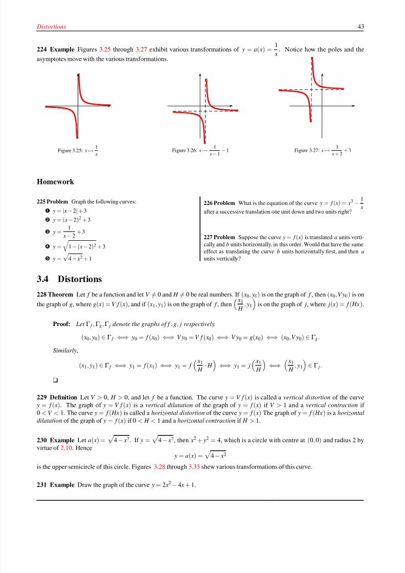
8/8/2019 Pre Calculus I
http://slidepdf.com/reader/full/pre-calculus-i 49/125
Distortions 43
224 Example Figures 3.25 through 3.27 exhibit various transformations of y = a( x) =1
x. Notice how the poles and the
asymptotes move with the various transformations.
Figure 3.25: x → 1
xFigure 3.26: x → 1
x− 1− 1 Figure 3.27: x → 1
x + 2+ 3
Homework
225 Problem Graph the following curves:
y = | x −2| + 3
y = ( x −2)2 + 3
y =1
x − 2+ 3
y =
1− ( x −2)2 + 3
y =
4− x2 + 1
226 Problem What is the equation of the curve y = f ( x) = x3 − 1 x
after a successive translation one unit down and two units right?
227 Problem Suppose the curve y = f ( x) is translated a units verti-
cally and b units horizontally, in this order. Would that have the same
effect as translating the curve b units horizontally first, and then a
units vertically?
3.4 Distortions
228 Theorem Let f be a function and let V = 0 and H = 0 be real numbers. If ( x0, y0) is on the graph of f , then ( x0,V y0) is onthe graph of g, where g( x) = V f ( x), and if ( x1, y1) is on the graph of f , then
x1
H , y1
is on the graph of j, where j( x) = f ( Hx).
Proof: Let Γ f ,Γ g,Γ j denote the graphs of f , g, j respectively.
( x0, y0) ∈ Γ f ⇐⇒ y0 = f ( x0) ⇐⇒ V y0 = V f ( x0) ⇐⇒ V y0 = g( x0) ⇐⇒ ( x0,V y0) ∈ Γ g.
Similarly,
( x1, y1) ∈ Γ f ⇐⇒ y1 = f ( x1) ⇐⇒ y1 = f
x1
H · H
⇐⇒ y1 = j
x1
H
⇐⇒
x1
H , y1
∈ Γ j.
u
229 Definition Let V > 0, H > 0, and let f be a function. The curve y = V f ( x) is called a vertical distortion of the curve y = f ( x). The graph of y = V f ( x) is a vertical dilatation of the graph of y = f ( x) if V > 1 and a vertical contraction if
0 < V < 1. The curve y = f ( Hx) is called a horizontal distortion of the curve y = f ( x) The graph of y = f ( Hx) is a horizontal
dilatation of the graph of y = f ( x) if 0 < H < 1 and a horizontal contraction if H > 1.
230 Example Let a( x) =
4 − x2. If y =
4 − x2, then x2 + y2 = 4, which is a circle with centre at (0, 0) and radius 2 by
virtue of 2.10. Hence
y = a( x) =
4 − x2
is the upper semicircle of this circle. Figures 3.28 through 3.33 shew various transformations of this curve.
231 Example Draw the graph of the curve y = 2 x2 − 4 x + 1.
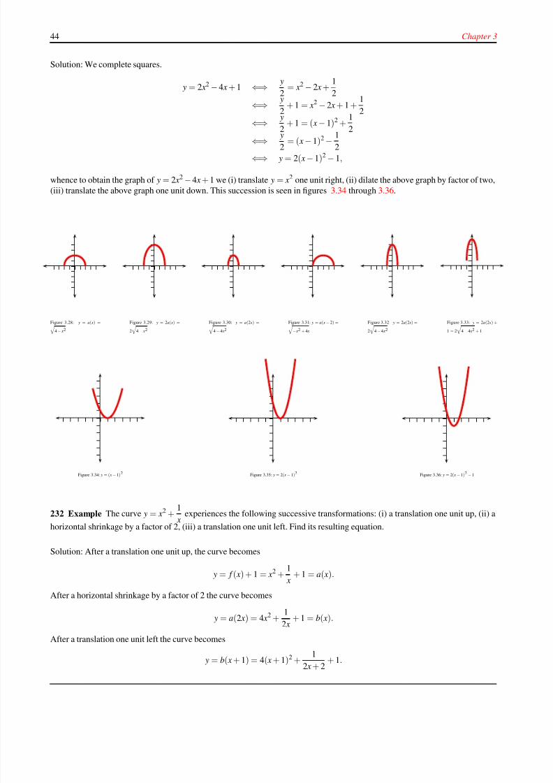
8/8/2019 Pre Calculus I
http://slidepdf.com/reader/full/pre-calculus-i 50/125
44 Chapter 3
Solution: We complete squares.
y = 2 x2 − 4 x + 1 ⇐⇒ y
2= x2 − 2 x +
1
2
⇐⇒ y
2+ 1 = x2 − 2 x + 1 +
1
2
⇐⇒ y
2+ 1 = ( x − 1)2 +
1
2
⇐⇒ y2
= ( x − 1)2 − 12
⇐⇒ y = 2( x − 1)2 − 1,
whence to obtain the graph of y = 2 x2 −4 x + 1 we (i) translate y = x2 one unit right, (ii) dilate the above graph by factor of two,
(iii) translate the above graph one unit down. This succession is seen in figures 3.34 through 3.36.
Figure 3.28: y = a( x) = 4− x2
Figure 3.29: y = 2a( x) =
2
4 − x2
Figure 3.30: y = a(2 x) = 4 −4 x2
Figure 3.31: y = a( x − 2) = − x2 + 4 x
Figure 3.32: y = 2a(2 x) =
2
4 −4 x2
Figure 3.33: y = 2a(2 x) +
1 = 2
4− 4 x2 + 1
Figure 3.34: y = ( x −1)2 Figure 3.35: y = 2( x − 1)2 Figure 3.36: y = 2( x −1)2 − 1
232 Example The curve y = x2 +1
xexperiences the following successive transformations: (i) a translation one unit up, (ii) a
horizontal shrinkage by a factor of 2, (iii) a translation one unit left. Find its resulting equation.
Solution: After a translation one unit up, the curve becomes
y = f ( x) + 1 = x2 +1
x+ 1 = a( x).
After a horizontal shrinkage by a factor of 2 the curve becomes
y = a(2 x) = 4 x2 +1
2 x+ 1 = b( x).
After a translation one unit left the curve becomes
y = b( x + 1) = 4( x + 1)2 +1
2 x + 2+ 1.
8/8/2019 Pre Calculus I
http://slidepdf.com/reader/full/pre-calculus-i 51/125
Reflexions 45
The required equation is thus
y = 4( x + 1)2 +1
2 x + 2+ 1 = 4 x2 + 8 x + 5 +
1
2 x + 2.
Homework
233 Problem Draw the graphs of the following curves:
y =x2
2
y =x2
2− 1
y = 2| x| + 1
y =2
x
y = x2
+ 4 x + 5
y = 2 x2 + 8 x
234 Problem The curve y =1
xexperiences the following successive
transformations: (i) a translation one unit left, (ii) a vertical dilatation
by a factor of 2, (iii) a translation one unit down. Find its resulting
equation and make a rough sketch of the resulting curve.
3.5 Reflexions
235 Theorem Let f be a function If ( x0, y0) is on the graph of f , then ( x0,− y0) is on the graph of g, where g( x) = − f ( x), and
if ( x1, y1) is on the graph of f , then (− x1, y1) is on the graph of j, where j( x) = f (− x).
Proof: Let Γ f ,Γ g,Γ j denote the graphs of f , g, j respectively.
( x0, y0) ∈ Γ f ⇐⇒ y0 = f ( x0) ⇐⇒ − y0 = − f ( x0) ⇐⇒ − y0 = g( x0) ⇐⇒ ( x0,− y0) ∈ Γ g.
Similarly,
( x1, y1) ∈ Γ f ⇐⇒ y1 = f ( x1) ⇐⇒ y1 = f (−(− x1)) ⇐⇒ y1 = j (− x1) ⇐⇒ (− x1, y1) ∈ Γ j.
u
236 Definition Let f be a function. The curve y = − f ( x) is said to be the reflexion of f about the x-axis and the curve
y = f (− x) is said to be the reflexion of f about the y-axis.
237 Example Figures 3.37 through 3.40 shew various reflexions about the axes.
238 Example Let f : R\{0} → R with
f ( x) = x +2
x− 1.
The curve y = f ( x) experiences the following successive transformations:
A reflexion about the x-axis.
A translation 3 units left.
A reflexion about the y-axis.
A vertical dilatation by a factor of 2.
Find the equation of the resulting curve. Note also how the domain of the function is affected by these transformations.
Solution:
A reflexion about the x-axis gives the curve
y = − f ( x) = 1− 2
x− x = a( x),
say, with Dom(a) = R\{0}.
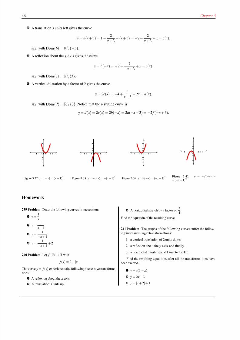
8/8/2019 Pre Calculus I
http://slidepdf.com/reader/full/pre-calculus-i 52/125
46 Chapter 3
A translation 3 units left gives the curve
y = a( x + 3) = 1 − 2
x + 3− ( x + 3) = −2 − 2
x + 3− x = b( x),
say, with Dom(b) = R\{−3}.
A reflexion about the y-axis gives the curve
y = b(− x) = −2 − 2
− x + 3+ x = c( x),
say, with Dom(c) = R\{3}.
A vertical dilatation by a factor of 2 gives the curve
y = 2c( x) = −4 +4
x − 3+ 2 x = d ( x),
say, with Dom(d ) = R\{3}. Notice that the resulting curve is
y = d ( x) = 2c( x) = 2b(− x) = 2a(− x + 3) = −2 f (− x + 3).
Figure 3.37: y = d ( x) = ( x− 1)2 Figure 3.38: y = −d ( x) =−( x−1)2 Figure 3.39: y = d (− x) = (− x−1)2 Figure 3.40: y = −d (− x) =−(− x− 1)2
Homework
239 Problem Draw the following curves in succession:
y =1
x
y =1
x + 1
y =
1
− x + 1
y =1
− x + 1+ 2
240 Problem Let f :R→R with
f ( x) = 2−| x|.The curve y = f ( x) experiences the following successive transforma-
tions:
A reflexion about the x-axis.
A translation 3 units up.
A horizontal stretch by a factor of 3
4.
Find the equation of the resulting curve.
241 Problem The graphs of the following curves suffer the follow-
ing successive, rigid transformations:
1. a vertical translation of 2 units down,
2. a reflexion about the y-axis, and finally,
3. a horizontal translation of 1 unit to the left.
Find the resulting equations after all the transformations have
been exerted.
y = x(1 − x)
y = 2 x − 3
y = | x + 2|+ 1
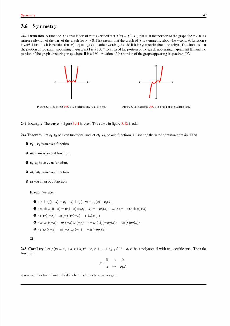
8/8/2019 Pre Calculus I
http://slidepdf.com/reader/full/pre-calculus-i 53/125
Symmetry 47
3.6 Symmetry
242 Definition A function f is even if for all x it is verified that f ( x) = f (− x), that is, if the portion of the graph for x < 0 is a
mirror reflexion of the part of the graph for x > 0. This means that the graph of f is symmetric about the y-axis. A function g
is odd if for all x it is verified that g(− x) = −g( x), in other words, g is odd if it is symmetric about the origin. This implies that
the portion of the graph appearing in quadrant I is a 180 ◦ rotation of the portion of the graph appearing in quadrant III, and the
portion of the graph appearing in quadrant II is a 180◦ rotation of the portion of the graph appearing in quadrant IV.
Figure 3.41: Example 243. The graph of an even function. Figure 3.42: Example 243. The graph of an odd function.
243 Example The curve in figure 3.41 is even. The curve in figure 3.42 is odd.
244 Theorem Let ε 1,ε 2 be even functions, and let ω 1,ω 2 be odd functions, all sharing the same common domain. Then
ε 1 ± ε 2 is an even function.
ω 1 ±ω 2 is an odd function.
ε 1 ·ε 2 is an even function.
ω 1 ·ω 2 is an even function.
ε 1 ·ω 1 is an odd function.
Proof: We have
(ε 1 ± ε 2)(− x) = ε 1(− x) ± ε 2(− x) = ε 1( x) ± ε 2( x).
(ω 1 ±ω 2)(− x) = ω 1(− x) ±ω 2(− x) = −ω 1( x) ∓ω 2( x) = −(ω 1 ±ω 2)( x)
(ε 1ε 2)(− x) = ε 1(− x)ε 2(− x) = ε 1( x)ε 2( x)
(ω 1ω 2)(
− x) = ω 1(
− x)ω 2(
− x) = (
−ω 1( x))(
−ω 2( x)) = ω 1( x)ω 2( x))
(ε 1ω 1)(− x) = ε 1(− x)ω 1(− x) = −ε 1( x)ω 1( x)
u
245 Corollary Let p( x) = a0 + a1 x + a2 x2 + a3 x
3 + · · · + an−1 xn−1 + an x
n be a polynomial with real coefficients. Then the
function
p :R → R
x → p( x)
is an even function if and only if each of its terms has even degree.
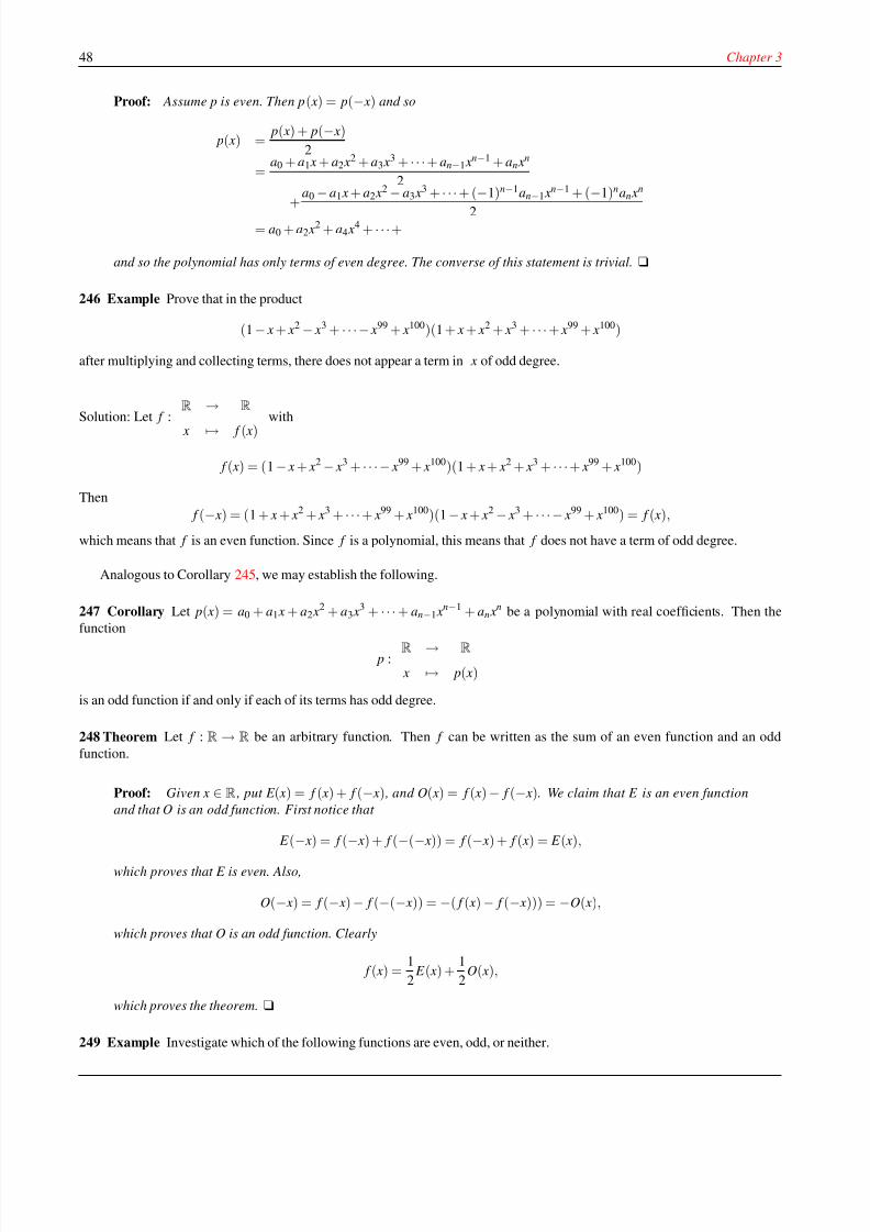
8/8/2019 Pre Calculus I
http://slidepdf.com/reader/full/pre-calculus-i 54/125
48 Chapter 3
Proof: Assume p is even. Then p( x) = p(− x) and so
p( x) =p( x) + p(− x)
2
=a0 + a1 x + a2 x
2 + a3 x3 + · · ·+ an−1 x
n−1 + an xn
2
+a0 − a1 x + a2 x
2 − a3 x3 + · · · + (−1)n−1an−1 x
n−1 + (−1)nan xn
2= a0 + a2 x
2 + a4 x4 + · · ·+
and so the polynomial has only terms of even degree. The converse of this statement is trivial.u
246 Example Prove that in the product
(1 − x + x2 − x3 + · · ·− x99 + x100)(1 + x + x2 + x3 + · · · + x99 + x100)
after multiplying and collecting terms, there does not appear a term in x of odd degree.
Solution: Let f :R → R
x → f ( x)with
f ( x) = (1 − x + x2 − x3 + · · ·− x99 + x100)(1 + x + x2 + x3 + · · ·+ x99 + x100)
Then
f (− x) = (1 + x + x2 + x3 + · · ·+ x99 + x100)(1 − x + x2 − x3 + · · ·− x99 + x100) = f ( x),
which means that f is an even function. Since f is a polynomial, this means that f does not have a term of odd degree.
Analogous to Corollary 245, we may establish the following.
247 Corollary Let p( x) = a0 + a1 x + a2 x2 + a3 x
3 + · · · + an−1 xn−1 + an x
n be a polynomial with real coefficients. Then the
function
p :R → R
x → p( x)
is an odd function if and only if each of its terms has odd degree.
248 Theorem Let f : R → R be an arbitrary function. Then f can be written as the sum of an even function and an odd
function.
Proof: Given x ∈ R , put E ( x) = f ( x) + f (− x) , and O( x) = f ( x) − f (− x). We claim that E is an even function
and that O is an odd function. First notice that
E (
− x) = f (
− x) + f (
−(
− x)) = f (
− x) + f ( x) = E ( x),
which proves that E is even. Also,
O(− x) = f (− x) − f (−(− x)) = −( f ( x) − f (− x))) = −O( x),
which proves that O is an odd function. Clearly
f ( x) =1
2 E ( x) +
1
2O( x),
which proves the theorem. u
249 Example Investigate which of the following functions are even, odd, or neither.
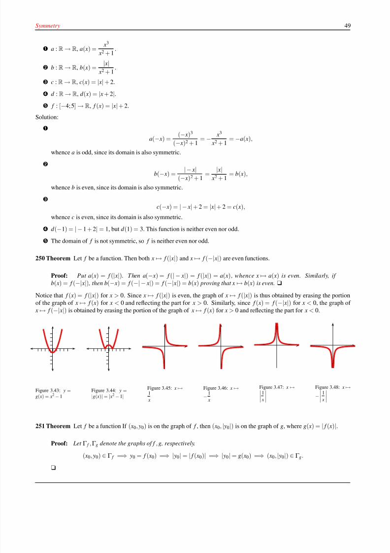
8/8/2019 Pre Calculus I
http://slidepdf.com/reader/full/pre-calculus-i 55/125
Symmetry 49
a : R→R, a( x) =x3
x2 + 1.
b : R→R, b( x) =| x|
x2 + 1.
c : R→ R, c( x) = | x| + 2.
d : R→ R, d ( x) = | x + 2|. f : [−4; 5] →R, f ( x) = | x|+ 2.
Solution:
a(− x) =(− x)3
(− x)2 + 1= − x3
x2 + 1= −a( x),
whence a is odd, since its domain is also symmetric.
b(− x) =|− x|
(− x)2 + 1=
| x| x2 + 1
= b( x),
whence b is even, since its domain is also symmetric.
c(− x) = |− x|+ 2 = | x|+ 2 = c( x),
whence c is even, since its domain is also symmetric.
d (−1) = |− 1 + 2| = 1, but d (1) = 3. This function is neither even nor odd.
The domain of f is not symmetric, so f is neither even nor odd.
250 Theorem Let f be a function. Then both x → f (| x|) and x → f (−| x|) are even functions.
Proof: Put a( x) = f (| x|). Then a(− x) = f (| − x|) = f (| x|) = a( x) , whence x → a( x) is even. Similarly, if
b( x) = f (−|
x|) , then b(
− x) = f (
−|− x|) = f (
−| x|) = b( x) proving that x
→b( x) is even. u
Notice that f ( x) = f (| x|) for x > 0. Since x → f (| x|) is even, the graph of x → f (| x|) is thus obtained by erasing the portion
of the graph of x → f ( x) for x < 0 and reflecting the part for x > 0. Similarly, since f ( x) = f (−| x|) for x < 0, the graph of
x → f (−| x|) is obtained by erasing the portion of the graph of x → f ( x) for x > 0 and reflecting the part for x < 0.
Figure 3.43: y =g( x) = x2 − 1
Figure 3.44: y =|g( x)| = | x2 − 1|
Figure 3.45: x →1
x
Figure 3.46: x →− 1
x
Figure 3.47: x →1
x
Figure 3.48: x →− 1
x
251 Theorem Let f be a function If ( x0, y0) is on the graph of f , then ( x0, | y0|) is on the graph of g, where g( x) = | f ( x)|.
Proof: Let Γ f ,Γ g denote the graphs of f , g, respectively.
( x0, y0) ∈ Γ f =⇒ y0 = f ( x0) =⇒ | y0| = | f ( x0)| =⇒ | y0| = g( x0) =⇒ ( x0, | y0|) ∈ Γ g.
u
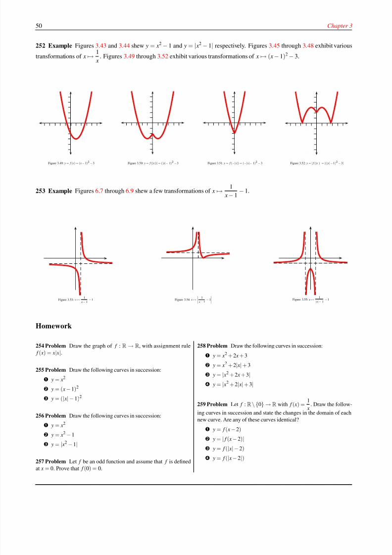
8/8/2019 Pre Calculus I
http://slidepdf.com/reader/full/pre-calculus-i 56/125
50 Chapter 3
252 Example Figures 3.43 and 3.44 shew y = x2 − 1 and y = | x2 − 1| respectively. Figures 3.45 through 3.48 exhibit various
transformations of x → 1
x. Figures 3.49 through 3.52 exhibit various transformations of x → ( x − 1)2 − 3.
Figure 3.49: y = f ( x) = ( x− 1)2 −3 Figure 3.50: y = f (| x|)| = (| x|− 1)2 −3 Figure 3.51: y = f (−| x|) = (−| x|− 1)2 −3 Figure 3.52: y = | f (| x|)| = |(| x|−1)2 −3|
253 Example Figures 6.7 through 6.9 shew a few transformations of x →1
x − 1 − 1.
Figure 3.53: x → 1
x− 1− 1 Figure 3.54: x →
1
x− 1− 1
Figure 3.55: x → 1
| x|− 1− 1
Homework
254 Problem Draw the graph of f : R → R, with assignment rule
f ( x) = x| x|.
255 Problem Draw the following curves in succession:
y = x2
y = ( x −1)2
y = (| x|−1)2
256 Problem Draw the following curves in succession:
y = x2
y = x2 −1
y = | x2 −1|
257 Problem Let f be an odd function and assume that f is defined
at x = 0. Prove that f (0) = 0.
258 Problem Draw the following curves in succession:
y = x2 + 2 x + 3
y = x2 + 2| x|+ 3
y = | x2 + 2 x + 3| y = | x2 + 2| x| + 3|
259 Problem Let f :R\{0} →R with f ( x) =1
x. Draw the follow-
ing curves in succession and state the changes in the domain of each
new curve. Are any of these curves identical?
y = f ( x −2)
y = | f ( x −2)| y = f (| x|− 2)
y = f (| x −2|)
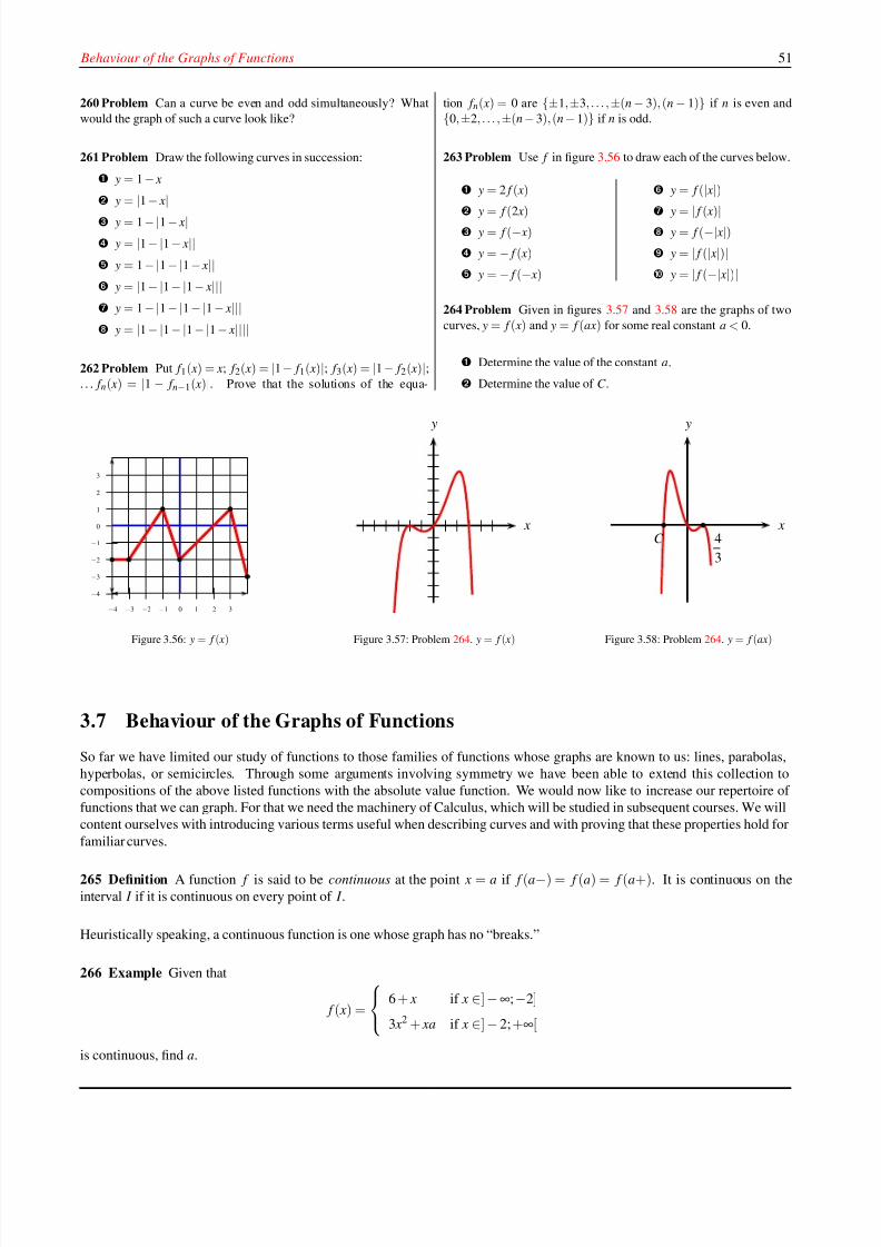
8/8/2019 Pre Calculus I
http://slidepdf.com/reader/full/pre-calculus-i 57/125
Behaviour of the Graphs of Functions 51
260 Problem Can a curve be even and odd simultaneously? What
would the graph of such a curve look like?
261 Problem Draw the following curves in succession:
y = 1− x
y =
|1
− x
| y = 1−|1− x| y = |1−|1− x|| y = 1−|1−|1− x|| y = |1−|1−|1− x||| y = 1−|1−|1−|1− x||| y = |1−|1−|1−|1− x||||
262 Problem Put f 1( x) = x; f 2( x) = |1− f 1( x)|; f 3( x) = |1− f 2( x)|;. . . f n( x) = |1 − f n−1( x)|. Prove that the solutions of the equa-
tion f n( x) = 0 are {±1,±3, . . . ,±(n − 3), (n − 1)} if n is even and
{0,±2, . . . ,±(n− 3),(n− 1)} if n is odd.
263 Problem Use f in figure 3.56 to draw each of the curves below.
y = 2 f ( x)
y = f (2 x)
y = f (− x)
y = − f ( x)
y = − f (− x)
y = f (| x|)
y = | f ( x)| y = f (−| x|) y = | f (| x|)| y = | f (−| x|)|
264 Problem Given in figures 3.57 and 3.58 are the graphs of two
curves, y = f ( x) and y = f (ax) for some real constant a < 0.
Determine the value of the constant a.
Determine the value of C .
−4
−3
−2
−1
0
1
2
3
−4 −3 −2 −1 0 1 2 3
Figure 3.56: y = f ( x)
x
y
Figure 3.57: Problem 264. y = f ( x)
x
y
4
3
C
Figure 3.58: Problem 264. y = f (ax)
3.7 Behaviour of the Graphs of Functions
So far we have limited our study of functions to those families of functions whose graphs are known to us: lines, parabolas,
hyperbolas, or semicircles. Through some arguments involving symmetry we have been able to extend this collection to
compositions of the above listed functions with the absolute value function. We would now like to increase our repertoire of
functions that we can graph. For that we need the machinery of Calculus, which will be studied in subsequent courses. We will
content ourselves with introducing various terms useful when describing curves and with proving that these properties hold for
familiar curves.
265 Definition A function f is said to be continuous at the point x = a if f (a−) = f (a) = f (a+). It is continuous on the
interval I if it is continuous on every point of I .
Heuristically speaking, a continuous function is one whose graph has no “breaks.”
266 Example Given that
f ( x) =
6 + x if x ∈]−∞;−2]
3 x2 + xa if x ∈]− 2; +∞[
is continuous, find a.
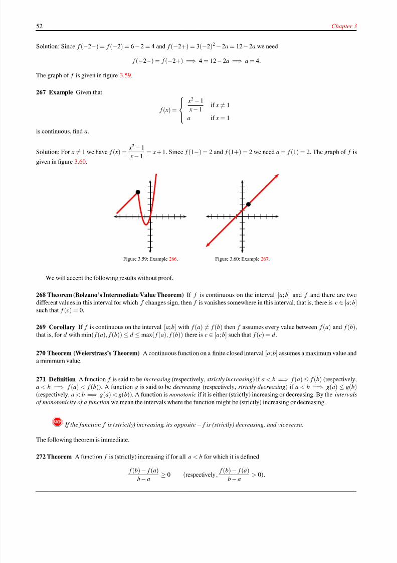
8/8/2019 Pre Calculus I
http://slidepdf.com/reader/full/pre-calculus-i 58/125
52 Chapter 3
Solution: Since f (−2−) = f (−2) = 6− 2 = 4 and f (−2+) = 3(−2)2 − 2a = 12 − 2a we need
f (−2−) = f (−2+) =⇒ 4 = 12 − 2a =⇒ a = 4.
The graph of f is given in figure 3.59.
267 Example Given that
f ( x) =
x2 − 1
x − 1if x = 1
a if x = 1
is continuous, find a.
Solution: For x = 1 we have f ( x) =x2 − 1
x − 1= x + 1. Since f (1−) = 2 and f (1+) = 2 we need a = f (1) = 2. The graph of f is
given in figure 3.60.
Figure 3.59: Example 266.
Figure 3.60: Example 267.
We will accept the following results without proof.
268 Theorem (Bolzano’s Intermediate Value Theorem) If f is continuous on the interval [a; b] and f and there are twodifferent values in this interval for which f changes sign, then f is vanishes somewhere in this interval, that is, there is c ∈ [a; b]such that f (c) = 0.
269 Corollary If f is continuous on the interval [a; b] with f (a) = f (b) then f assumes every value between f (a) and f (b),
that is, for d with min( f (a), f (b)) ≤ d ≤ max( f (a), f (b)) there is c ∈ [a; b] such that f (c) = d .
270 Theorem (Weierstrass’s Theorem) A continuous function on a finite closed interval [a; b] assumes a maximum value and
a minimum value.
271 Definition A function f is said to be increasing (respectively, strictly increasing) if a < b =⇒ f (a) ≤ f (b) (respectively,
a < b =⇒ f (a) < f (b)). A function g is said to be decreasing (respectively, strictly decreasing) if a < b =⇒ g(a) ≤ g(b)(respectively, a < b =⇒ g(a) < g(b)). A function is monotonic if it is either (strictly) increasing or decreasing. By the intervals
of monotonicity of a function we mean the intervals where the function might be (strictly) increasing or decreasing.
! If the function f is (strictly) increasing, its opposite− f is (strictly) decreasing, and viceversa.
The following theorem is immediate.
272 Theorem A function f is (strictly) increasing if for all a < b for which it is defined
f (b) − f (a)
b− a≥ 0 (respectively,
f (b)− f (a)
b − a> 0).
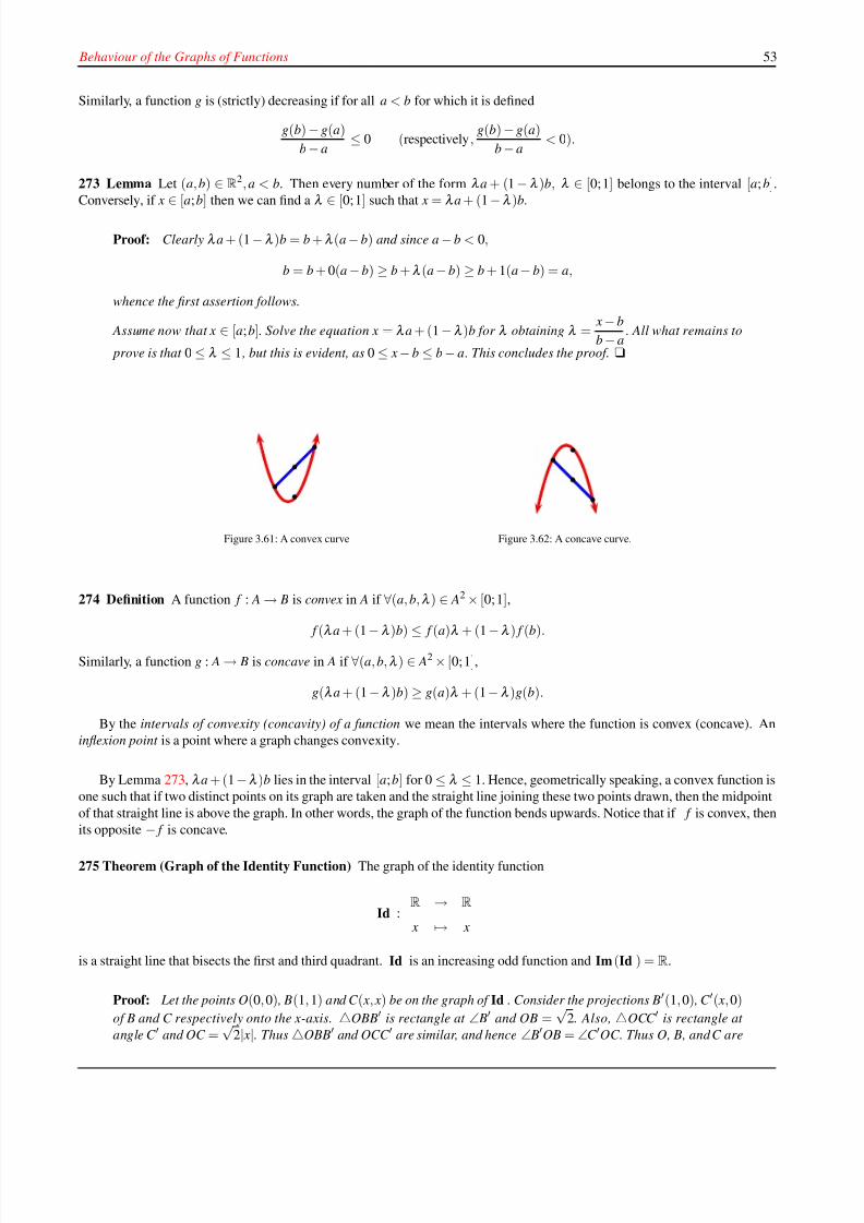
8/8/2019 Pre Calculus I
http://slidepdf.com/reader/full/pre-calculus-i 59/125
Behaviour of the Graphs of Functions 53
Similarly, a function g is (strictly) decreasing if for all a < b for which it is defined
g(b) − g(a)
b − a≤ 0 (respectively,
g(b) − g(a)
b − a< 0).
273 Lemma Let (a, b) ∈ R2, a < b. Then every number of the form λ a + (1 −λ )b, λ ∈ [0; 1] belongs to the interval [a; b].Conversely, if x
∈[a; b] then we can find a λ
∈[0; 1] such that x = λ a + (1
−λ )b.
Proof: Clearly λ a + (1 −λ )b = b +λ (a − b) and since a − b < 0,
b = b + 0(a − b) ≥ b +λ (a − b) ≥ b + 1(a− b) = a,
whence the first assertion follows.
Assume now that x ∈ [a; b]. Solve the equation x = λ a + (1 −λ )b for λ obtaining λ =x − b
b − a. All what remains to
prove is that 0 ≤ λ ≤ 1 , but this is evident, as 0 ≤ x − b ≤ b − a. This concludes the proof. u
Figure 3.61: A convex curve
Figure 3.62: A concave curve.
274 Definition A function f : A → B is convex in A if ∀(a, b,λ ) ∈ A2 × [0; 1],
f (λ a + (1 −λ )b) ≤ f (a)λ + (1 −λ ) f (b).
Similarly, a function g : A → B is concave in A if ∀(a, b,λ ) ∈ A2 × [0; 1],
g(λ a + (1 −λ )b) ≥ g(a)λ + (1−λ )g(b).
By the intervals of convexity (concavity) of a function we mean the intervals where the function is convex (concave). An
inflexion point is a point where a graph changes convexity.
By Lemma 273, λ a + (1−λ )b lies in the interval [a; b] for 0 ≤ λ ≤ 1. Hence, geometrically speaking, a convex function is
one such that if two distinct points on its graph are taken and the straight line joining these two points drawn, then the midpoint
of that straight line is above the graph. In other words, the graph of the function bends upwards. Notice that if f is convex, then
its opposite
− f is concave.
275 Theorem (Graph of the Identity Function) The graph of the identity function
Id :R → R
x → x
is a straight line that bisects the first and third quadrant. Id is an increasing odd function and Im (Id ) = R.
Proof: Let the points O(0, 0) , B(1, 1) and C ( x, x) be on the graph of Id . Consider the projections B′(1, 0) , C ′( x, 0)
of B and C respectively onto the x-axis. △OBB′ is rectangle at ∠ B′ and OB =√
2. Also, △OCC ′ is rectangle at
angle C ′ and OC =√
2| x|. Thus △OBB′ and OCC ′ are similar, and hence ∠ B′OB =∠C ′OC. Thus O, B, and C are
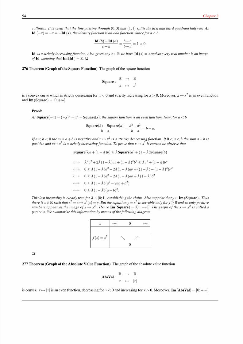
8/8/2019 Pre Calculus I
http://slidepdf.com/reader/full/pre-calculus-i 60/125
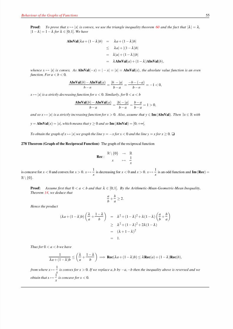
8/8/2019 Pre Calculus I
http://slidepdf.com/reader/full/pre-calculus-i 61/125
Behaviour of the Graphs of Functions 55
Proof: To prove that x → | x| is convex, we use the triangle inequality theorem 60 and the fact that |λ | = λ ,|1 −λ | = 1 −λ for λ ∈ [0; 1]. We have
AbsVal(λ a + (1 −λ )b) = |λ a + (1 −λ )b|≤ |λ a|+ |(1−λ )b|= λ
|a|
+ (1−λ )
|b|
= λ AbsVal(a) + (1 −λ )AbsVal(b),
whence x → | x| is convex. As AbsVal(− x) = | − x| = | x| = AbsVal( x) , the absolute value function is an even
function. For a < b < 0 ,
AbsVal(b) − AbsVal(a)
b − a=
|b|− |a|b − a
=−b − (−a)
b − a= −1 < 0,
x → | x| is a strictly decreasing function for x < 0. Similarly, for 0 < a < b
AbsVal(b) − AbsVal(a)
b − a=
|b|− |a|b − a
=b− a
b− a= 1 > 0,
and so x → | x| is a strictly increasing function for x > 0. Also, assume that y ∈ Im (AbsVal). Then ∃ x ∈ R with
y = AbsVal( x) = | x| , which means that y ≥ 0 and so Im (AbsVal) = [0; +∞[.
To obtain the graph of x → | x| we graph the line y = − x for x < 0 and the line y = x for x ≥ 0. u
278 Theorem (Graph of the Reciprocal Function) The graph of the reciprocal function
Rec :R\{0} → R
x → 1
x
is concave for x < 0 and convex for x > 0. x → 1 x
is decreasing for x < 0 and x > 0. x → 1 x
is an odd function and Im (Rec) =
R\{0}.
Proof: Assume first that 0 < a < b and that λ ∈ [0; 1]. By the Arithmetic-Mean-Geometric-Mean Inequality,
Theorem 14 , we deduce that a
b+
b
a≥ 2.
Hence the product
(λ a + (1 −λ )b)
λ
a+
1 −λ
b
= λ 2 + (1−λ )2 +λ (1 −λ )
a
b+
b
a
≥λ 2 + (1
−λ )2 + 2λ (1
−λ )
= (λ + 1 −λ )2
= 1.
Thus for 0 < a < b we have
1
λ a + (1 −λ )b≤λ
a+
1 −λ
b
=⇒ Rec(λ a + (1 −λ )b) ≤ λ Rec(a) + (1 −λ )Rec(b),
from where x → 1
xis convex for x > 0. If we replace a, b by −a,−b then the inequality above is reversed and we
obtain that x → 1
xis concave for x < 0.
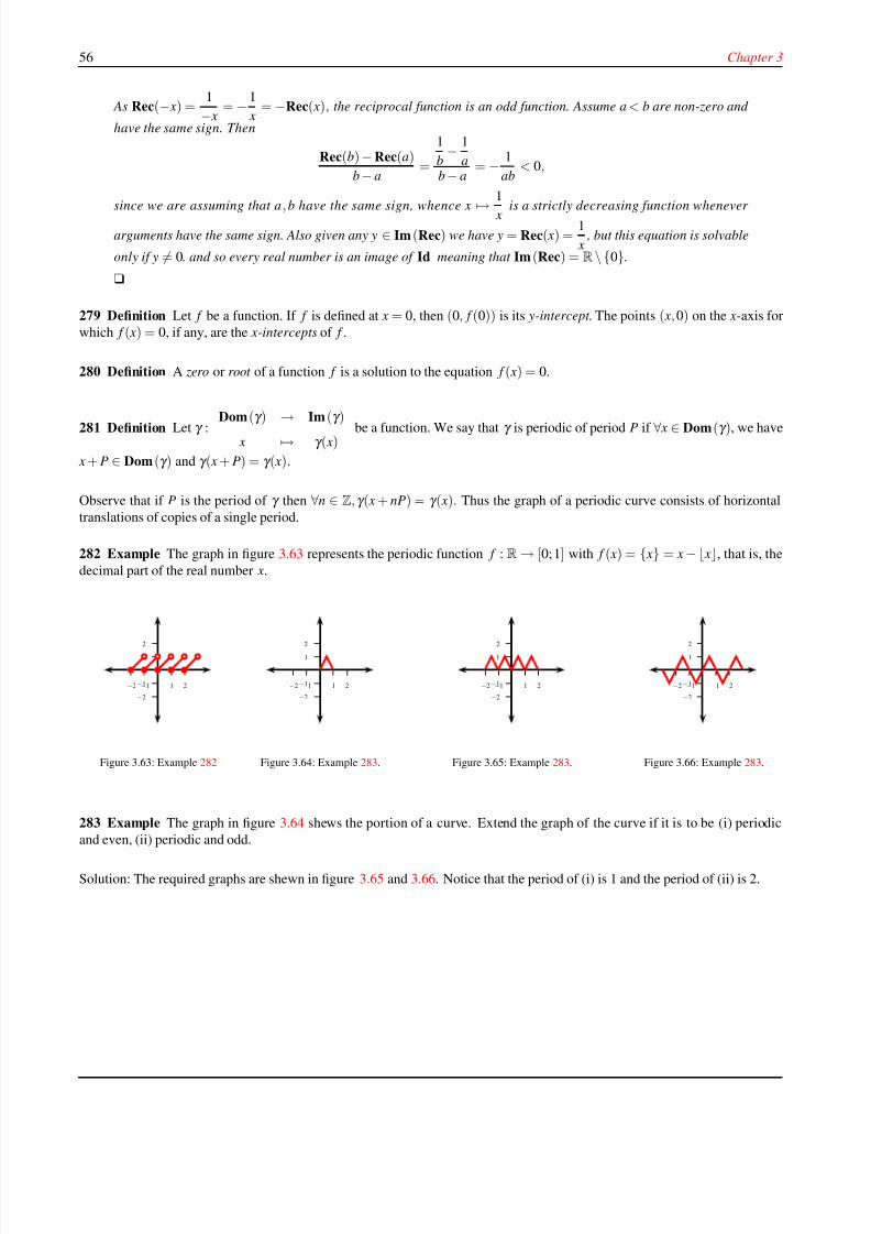
8/8/2019 Pre Calculus I
http://slidepdf.com/reader/full/pre-calculus-i 62/125
56 Chapter 3
As Rec(− x) =1
− x= −1
x= −Rec( x) , the reciprocal function is an odd function. Assume a< b are non-zero and
have the same sign. Then
Rec(b) − Rec(a)
b− a=
1
b− 1
ab− a
= − 1
ab< 0,
since we are assuming that a, b have the same sign, whence x→
1
xis a strictly decreasing function whenever
arguments have the same sign. Also given any y ∈ Im (Rec) we have y = Rec( x) =1
x , but this equation is solvable
only if y = 0. and so every real number is an image of Id meaning that Im (Rec) = R\{0}.
u
279 Definition Let f be a function. If f is defined at x = 0, then (0, f (0)) is its y-intercept . The points ( x, 0) on the x-axis for
which f ( x) = 0, if any, are the x-intercepts of f .
280 Definition A zero or root of a function f is a solution to the equation f ( x) = 0.
281 Definition Let γ :Dom(γ )
→Im (γ )
x → γ ( x)be a function. We say that γ is periodic of period P if ∀ x ∈ Dom(γ ), we have
x + P ∈ Dom(γ ) and γ ( x + P) = γ ( x).
Observe that if P is the period of γ then ∀n ∈ Z,γ ( x + nP) = γ ( x). Thus the graph of a periodic curve consists of horizontal
translations of copies of a single period.
282 Example The graph in figure 3.63 represents the periodic function f : R→ [0; 1] with f ( x) = { x} = x −⌊ x⌋, that is, the
decimal part of the real number x.
1
2
−1
−2
1 2−1−2
Figure 3.63: Example 282
1
2
−1
−2
1 2−1−2
Figure 3.64: Example 283.
1
2
−1
−2
1 2−1−2
Figure 3.65: Example 283.
1
2
−1
−2
1 2−1−2
Figure 3.66: Example 283.
283 Example The graph in figure 3.64 shews the portion of a curve. Extend the graph of the curve if it is to be (i) periodic
and even, (ii) periodic and odd.
Solution: The required graphs are shewn in figure 3.65 and 3.66. Notice that the period of (i) is 1 and the period of (ii) is 2.
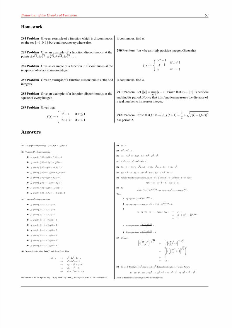
8/8/2019 Pre Calculus I
http://slidepdf.com/reader/full/pre-calculus-i 63/125
Behaviour of the Graphs of Functions 57
Homework
284 Problem Give an example of a function which is discontinuous
on the set {−1, 0, 1} but continuous everywhere else.
285 Problem Give an example of a function discontinuous at the
points ±3
√1,±3
√2,±3
√3,±3
√4,±3
√5, . . ..
286 Problem Give an example of a function r discontinuous at the
reciprocal of every non-zero integer.
287 Problem Give an example of a function discontinuous at the odd
integers.
288 Problem Give an example of a function discontinuous at the
square of every integer.
289 Problem Given that
f ( x) = x2 −1 if x ≤ 1
2 x + 3a if x > 1
is continuous, find a.
290 Problem Let n be a strictly positive integer. Given that
f ( x) =
xn − 1
x− 1if x = 1
a if x = 1
is continuous, find a.
291 Problem Let || x|| = minn∈Z
| x − n|. Prove that x → || x|| is periodic
and find its period. Notice that this function measures the distance of
a real number to its nearest integer.
292 Problem Prove that f :R→R, f (t + 1) = 12
+ f (t )− ( f (t ))2
has period 2.
Answers
185 The graph is in figure ??. f (−1) = 3, f (0) = 1, f (1) = 1.
186 There are 23 = 8 such functions:
f 1 given by f 1(0) = f 1(1) = f 1(2) = −1
f 2 given by f 2(0) = 1, f 2(1) = f 2(2) = −1
f 3 given by f 3(0) = f 3(1) = −1, f 3(2) = 1
f 4 given by f 4(0) = −1, f 4(1) = 1, f 4 (2) = −1
f 5 given by f 5(0) = f 5(1) = f 5(2) = 1
f 6 given by f 6(0) = −1, f 6(1) = f 6(2) = 1
f 7 given by f 7(0) = f 7(1) = 1, f 7(2) = −1
f 8 given by f 8(0) = 1, f 8(1) = −1, f 8 (2) = 1
187 There are 32 = 9 such functions:
f 1 given by f 1(−1) = f 1(1) = 0
f 2 given by f 2(−1) = f 2(1) = 1
f 3 given by f 3(−1) = f 3(1) = 2
f 4 given by f 4(−1) = 0, f 4(1) = 1
f 5 given by f 5(
−1) = 0, f 5(1) = 2
f 6 given by f 6(−1) = 1, f 6(1) = 2
f 7 given by f 7(−1) = 1, f 7(1) = 0
f 8 given by f 8(−1) = 2, f 8(1) = 0
f 9 given by f 9(−1) = 2, f 9(1) = 1
188 We must look for all x ∈ Dom( f ) such that s( x) = x. Thus
s( x) = x =⇒ x5 − 2 x3 + 2 x = x
=⇒ x5 − 2 x3 + x = 0
=⇒ x( x4 −2 x2 + 1) = 0
=⇒ x( x2 −1)2 = 0
=⇒ x( x + 1)2( x −1)2 = 0.
The solutions to this last equation are {−1, 0, 1}. Since −1 ∈ Dom(s), the only fixed points of s are x = 0 and x = 1.
189 4 x − 2
190 6 x2 + 2h2 − 6
191 a(3) = 6; x2 + x −6; 24 −11 x −10 x2 + 2 x3 + x4
192 7, x2 − 2 x −1, x4 −4 x3 + 8 x + 2
193 h( x− 1) = −11 + 7 x− x2 ; h( x) = −5 + 5 x− x2 ; h( x + 1) = −1 + 3 x − x2
194 f ( x) = x2 − 2 x + 1; f ( x + 2) = x2 + 2 x + 1; f ( x −2) = x2 − 6 x + 9
195 Rename the independent variable, say h(1− s) = 2s. Now, if 1 −s = 3 x then s = 1− 3 x. Hence
h(3 x) = h(1− s) = 2s = 2(1 −3 x) = 2 −6 x.
196 Put p( x) = (1− x2 + x4)2003 = a0 + a1 x + a2 x2 + ·· ·+ a8012 x8012 .
Then
a0 = p(0) = (1 − 02 + 04)2003 = 1.
a0 + a1 + a2 + ·· ·+ a8012 = p(1) = (1 −12 + 14)2003 = 1.
a0 −a1 + a2 −a3 + · · ·− a8011 + a8012 = p(−1)
= (1 −(−1)2 +(−1)4)2003
= 1.
The required sum isp(1)+ p(−1)
2
= 1.
The required sum isp(1)− p(−1)
2= 0.
197 We have f
27 + y3
y3
27 y
=
f
3
y
3+ 1
3
3 y
=
f
3
y
3+ 1
3 y
3
= 53
= 125.
198 Let y = 0. Then 2g( x) = 2 x2 , that is, g( x) = x2 . Let us check that g( x) = x2 works. We have
g( x + y)+ g( x− y) = ( x + y)2 +( x− y)2 = x2 + 2 xy + y2 + x2 −2 xy + y2 = 2 x2 + 2 y2 ,
which is the functional equation given. Our choice of g works.
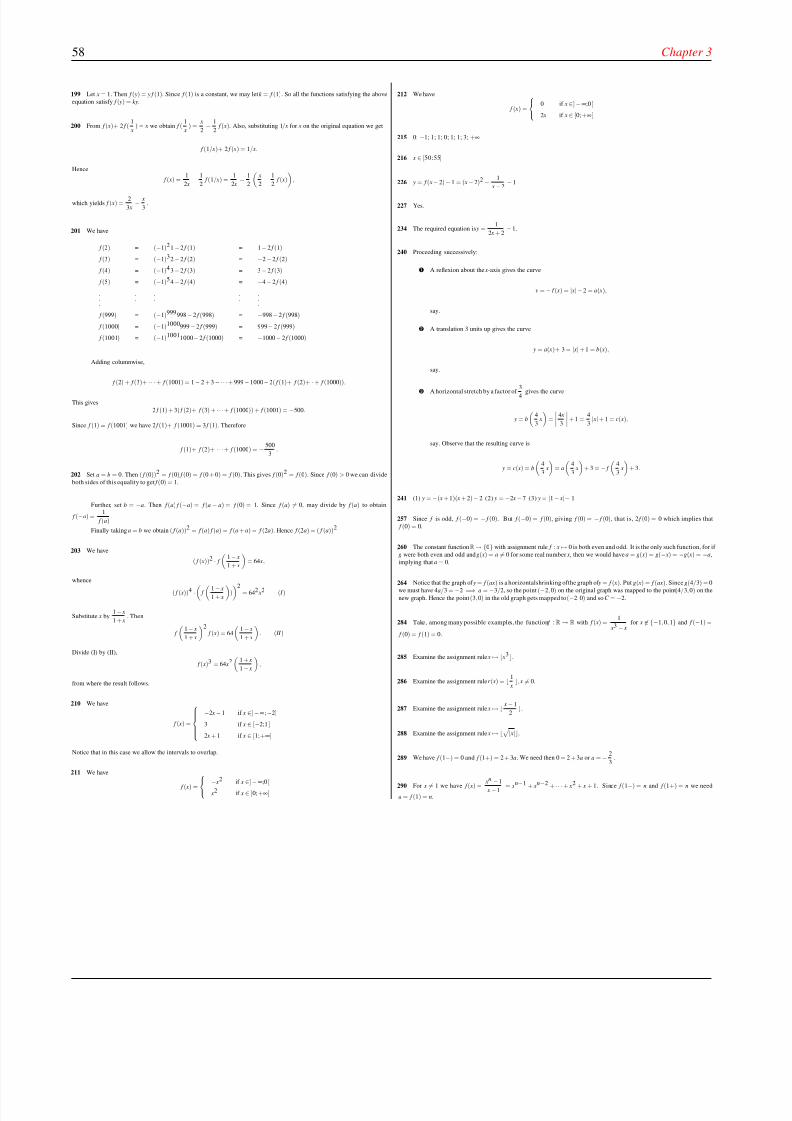
8/8/2019 Pre Calculus I
http://slidepdf.com/reader/full/pre-calculus-i 64/125
58 Chapter 3
199 Let x = 1. Then f ( y) = y f (1). Since f (1) is a constant, we may let k = f (1). So all the functions satisfying the above
equation satisfy f ( y) = ky.
200 From f ( x)+ 2 f (1
x) = x we obtain f (
1
x) =
x
2− 1
2f ( x). Also, substituting 1/ x for x on the original equation we get
f (1/ x)+ 2 f ( x) = 1/ x.
Hence
f ( x) =1
2 x− 1
2f (1/ x) =
1
2 x− 1
2
x
2− 1
2f ( x)
,
which yields f ( x) =2
3 x− x
3.
201 We have
f (2) = (−1)2 1 −2 f (1) = 1− 2 f (1)
f (3) = (−1)3 2 −2 f (2) = −2 −2 f (2)
f (4) = (−1)4 3 −2 f (3) = 3− 2 f (3)
f (5) = (−1)5 4 −2 f (4) = −4 −2 f (4)
.
.
.
.
.
.
.
.
.
.
.
.
.
.
.
f (999) = (−1)999 998 − 2 f (998) = −998 −2 f (998)
f (1000) = (−1)1000999 −2 f (999) = 999− 2 f (999)
f (1001) = (−1)10011000− 2 f (1000) = −1000 − 2 f (1000)
Adding columnwise,
f (2) + f (3)+
·· ·+ f (1001) = 1
−2 + 3
−···+ 999
−1000
−2( f (1)+ f (2)+
·+ f (1000)).
This gives
2 f (1) + 3( f (2)+ f (3) + ·· ·+ f (1000)) + f (1001) = −500.
Since f (1) = f (1001) we have 2 f (1)+ f (1001) = 3 f (1). Therefore
f (1)+ f (2)+ ·· ·+ f (1000) = − 500
3.
202 Set a = b = 0. Then ( f (0))2 = f (0) f (0) = f (0 + 0) = f (0). This gives f (0)2 = f (0). Since f (0) > 0 we can divide
both sides of this equality to get f (0) = 1.
Further, set b = −a. Then f (a) f (−a) = f (a − a) = f (0) = 1. Since f (a) = 0, may divide by f (a) to obtain
f (−a) =1
f (a).
Finally taking a = b we obtain ( f (a))2 = f (a) f (a) = f (a + a) = f (2a). Hence f (2a) = ( f (a))2
203 We have
( f ( x))2 · f
1 − x
1 + x
= 64 x,
whence
( f ( x))4 ·
f
1 − x
1 + x
)
2= 642 x2 ( I )
Substitute x by1 − x
1 + x. Then
f
1 − x
1 + x
2 f ( x) = 64
1 − x
1 + x
. ( II )
Divide (I) by (II),
f ( x)3 = 64 x2
1 + x
1 − x
,
from where the result follows.
210 We have
f ( x) =
−2 x− 1 if x ∈] −∞;−2]
3 if x ∈ [−2;1 ]
2 x + 1 if x ∈ [1; +∞[
Notice that in this case we allow the intervals to overlap.
211 We have
f ( x) =
− x2 if x ∈]−∞;0 [
x2 if x ∈ [0; +∞[
212 We have
f ( x) =
0 if x ∈]−∞;0 [
2 x if x ∈ [0; +∞[
215 0; −1; 1; 1; 0; 1; 1; 3; +∞
216 x ∈ [50;55[
226 y = f ( x− 2)− 1 = ( x − 2)2 − 1
x
−2
− 1
227 Yes.
234 The required equation is y =1
2 x + 2−1.
240 Proceeding successively:
A reflexion about the x-axis gives the curve
y = − f ( x) = | x|−2 = a( x),
say.
A translation 3 units up gives the curve
y = a( x)+ 3 = | x| + 1 = b( x),
say.
A horizontal stretch by a factor of 34
gives the curve
y = b
4
3x
=
4 x
3
+ 1 =4
3| x|+ 1 = c( x),
say. Observe that the resulting curve is
y = c( x) = b
4
3x
= a
4
3x
+ 3 = − f
4
3x
+ 3.
241 (1) y = −( x + 1)( x + 2)− 2 (2) y = −2 x −7 (3) y = |1 − x|− 1
257 Since f is odd, f (−0) = − f (0). But f (−0) = f (0), giving f (0) = − f (0), that is, 2 f (0) = 0 which implies that
f (0) = 0.
260 The constant function R→ {0} with assignment rule f : x → 0 is both even and odd. It is the only such function, for if g were both even and odd and g( x) = a = 0 for some real number x, then we would have a = g( x) = g(− x) = −g( x) = −a,
implying that a = 0.
264 Notice that the graph of y = f (ax) is a horizontalshrinking ofthe graph of y = f ( x). Put g( x) = f (ax). Since g(4/3) = 0we must have 4a/3 = −2 =⇒ a = −3/2, so the point (−2, 0) on the original graph was mapped to the point (4/3, 0) on the
new graph. Hence the point (3, 0) in the old graph gets mapped to (−2, 0) and so C = −2.
284 Take, among many possible examples, the function f : R→ R with f ( x) =1
x3 − xfor x ∈ {−1, 0, 1} and f (−1) =
f (0) = f (1) = 0.
285 Examine the assignment rule x → ⌊ x3⌋.
286 Examine the assignment rule r ( x) = ⌊ 1
x⌋, x = 0.
287 Examine the assignment rule x → ⌊ x −1
2⌋.
288 Examine the assignment rule x → ⌊
| x|⌋.
289 We have f (1−) = 0 and f (1+) = 2 + 3a. We need then 0 = 2 + 3a or a = − 2
3.
290 For x = 1 we have f ( x) =xn −1
x −1= xn−1 + xn−2 + ·· · + x2 + x + 1. Since f (1−) = n and f (1+) = n we need
a = f (1) = n.
8/8/2019 Pre Calculus I
http://slidepdf.com/reader/full/pre-calculus-i 65/125
Chapter 4Functions II: Domains and Images
4.1 Natural Domain of an Assignment Rule
293 Definition The natural domain of an assignment rule is the largest set of real number inputs that will give a real number
output of a given assignment rule.
! For the algebraic combinations that we are dealing with, we must then worry about having non-vanishing
denominators and taking even-indexed roots of positive real numbers.
294 Example Find the natural domain of the rule x → 1
x2 − x − 6.
Solution: In order for the output to be a real number, the denominator must not vanish. We must have x2 − x − 6 = ( x + 2)( x −3) = 0, and so x = −2 nor x = 3. Thus the natural domain of this rule is R\{−2, 3}.
295 Example Find the natural domain of x → 1 x4 − 16
.
Solution: Since x4 − 16 = ( x2 − 4)( x2 + 4) = ( x + 2)( x − 2)( x2 + 4), the rule is undefined when x = −2 or x = 2. The natural
domain is thus R\{−2, +2}.
296 Example Find the natural domain for the rule f ( x) =2
4 −| x| .
Solution: The denominator must not vanish, hence x = ±4. The natural domain of this rule is thus R\{−4, 4}.
297 Example Find the natural domain of the rule f ( x) =√
x + 3
Solution: In order for the output to be a real number, the quantity under the square root must be positive, hence x + 3 ≥ 0 =⇒ x ≥ −3 and the natural domain is the interval [−3; +∞[.
298 Example Find the natural domain of the rule g( x) =2√
x + 3
Solution: The denominator must not vanish, and hence the quantity under the square root must be positive, therefore x > −3
and the natural domain is the interval ] − 3+;∞[.
299 Example Find the natural domain of the rule x → 4√
x2.
59
8/8/2019 Pre Calculus I
http://slidepdf.com/reader/full/pre-calculus-i 66/125
60 Chapter 4
Solution: Since for all real numbers x2 ≥ 0, the natural domain of this rule is R.
300 Example Find the natural domain of the rule x → 4
− x2.
Solution: Since for all real numbers − x2 ≤ 0, the quantity under the square root is a real number only when x = 0, whence the
natural domain of this rule is {0}.
301 Example Find the natural domain of the rule x → 1√ x2
.
Solution: The denominator vanishes when x = 0. Otherwise for all real numbers, x = 0, we have x2 > 0. The natural domain of
this rule is thus R\{0}.
302 Example Find the natural domain of the rule x → 1√− x2.
Solution: The denominator vanishes when x = 0. Otherwise for all real numbers, x = 0, we have − x2 < 0. Thus
− x2 is only
a real number when x = 0, and in that case, the denominator vanishes. The natural domain of this rule is thus the empty set ∅.
303 Example Find the natural domain of the assignment rule
x → √1 − x +
1√1 + x
.
Solution: We need simultaneously 1− x ≥ 0 (which implies that x ≤ 1) and 1 + x > 0 (which implies that x > −1), so x ∈]−1; 1].
304 Example Find the largest subset of real numbers where the assignment rule x →
x2 − x − 6 gives real number outputs.
Solution: The quantity x2 − x − 6 = ( x + 2)( x − 3) under the square root must be positive. Studying the sign diagram
x ∈ ]−∞;−2] [−2; 3] [3; +∞[
signum( x + 2) = − + +
signum( x− 3) = − − +
signum(( x + 2)( x − 2)) = + − +
we conclude that the natural domain of this formula is the set ]−∞;−2] ∪ [3; +∞[.
305 Example Find the natural domain for the rule f ( x) =1√
x2 − x − 6.
The denominator must not vanish, so the quantity under the square root must be positive. By the preceding problem this happenswhen x ∈] −∞;−2[ ∪ ]3; +∞[.
306 Example Find the natural domain of the rule x →
x2 + 1.
Solution: Since ∀ x ∈ R we have x2 + 1 ≥ 1, the square root is a real number for all real x. Hence the natural domain is R.
307 Example Find the natural domain of the rule x →
x2 + x + 1.
Solution: The discriminant of x2 + x + 1 = 0 is 12 − 4(1)(1) < 0. Since the coefficient of x2 is 1 > 0, the expression x2 + x + 1
is always positive, meaning that the required natural domain is all of R.
8/8/2019 Pre Calculus I
http://slidepdf.com/reader/full/pre-calculus-i 67/125
Algebra of Functions 61
Aliter: Observe that
x2 + x + 1 =
x +
1
2
2
+3
4≥ 3
4,
the square root is a real number for all real x. Hence the natural domain is R.
Homework
308 Problem Below are given some assignment rules. Verify that
the accompanying set is the natural domain of the assignment rule.
Assignment Rule Natural Domain
x →
(1− x)( x + 3) x ∈ [−3; 1].
x →
1− x
x + 3x ∈] − 3; 1]
x → x + 3
1− x x ∈ [−3; 1[
x →
1
( x + 3)(1− x)x ∈] − 3; 1[
309 Problem Find the natural domain for the given assignment
rules.
x →
1 1 + | x| x → 4
5−| x|
x → 3
5−| x| x → 1
x2 + 2 x + 2
x → 1√ x2 − 2 x −2
x →
1
| x− 1|+ | x + 1|
x →√− x
x2 − 1
x →√
1− x2
1−| x| x → √
x +√− x
310 Problem Below are given some assignment rules. Verify that
the accompanying set is the natural domain of the assignment rule.
Assignment Rule Natural Domain
x →
x
x2 −9x ∈]− 3; 0]
]3; +∞[
x →
−| x| x = 0
x →
−|| x|− 2| x ∈ {−2,2}
x →
1
x x ∈]0; +∞[
x →
1
x2x ∈R\{0}
x → 1
− x
x ∈]−∞; 0[
x →
1
−| x| ∅ (the empty set)
x → 1
x√
x + 1 x ∈]− 1; 0[
]0; +∞[
x → √1 + x +
√1− x [−1; 1]
311 Problem Find the natural domain for the rule
f ( x) =
x3 − 12 x.
312 Problem Find the natural domain of the rule
x → 1√ x2
−2 x
−2
.
313 Problem Find the natural domain for the following rules.
x →
−( x + 1)2,
x → 1 −( x + 1)2
f ( x) =
x1/2
√ x4 − 13 x2 + 36
g( x) =4√
3− x√ x4 − 13 x2 + 36
h( x) =1√
x6 − 13 x4 + 36 x2
j( x) =1√
x5 − 13 x3 + 36 x
k ( x) =1
| x4 − 13 x2 + 36|
4.2 Algebra of Functions
314 Definition Let f : Dom( f ) → R and g : Dom(g) →R. Then Dom( f ± g) = Dom( f ) ∩ Dom(g) and the sum
(respectively, difference) function f + g (respectively, f − g) is given by
f ± g :Dom( f ) ∩ Dom(g) → R
x → f ( x) ± g( x).
In other words, if x belongs both to the domain of f and g, then
( f ± g)( x) = f ( x)± g( x).
8/8/2019 Pre Calculus I
http://slidepdf.com/reader/full/pre-calculus-i 68/125
62 Chapter 4
315 Definition Let f : Dom( f ) → R and g : Dom(g) →R. Then Dom( f g) = Dom( f ) ∩ Dom(g) and the product function
f g is given by
f g :Dom( f )∩ Dom(g) → R
x → f ( x) · g( x).
In other words, if x belongs both to the domain of f and g, then
( f g)( x) = f ( x) · g( x).
316 Example Let
f :[−1; 1] → R
x → x2 + 2 x, g :
[0; 2] → R
x → 3 x + 2.
Find
Dom( f ± g)
Dom( f g)
( f + g)(−1)
( f + g)(1)
( f g)(1)
( f − g)(0)
( f + g)(2)
Solution: We have
Dom( f ± g) = Dom( f ) ∩ Dom(g) = [−1; 1]∩ [0; 2] =[0; 1].
Dom( f g) is also Dom( f ) ∩ Dom(g) = [0; 1].
Since−
1∈
[0; 1], ( f + g)(−
1) is undefined.
( f + g)(1) = f (1) + g(1) = 3 + 5 = 8.
( f g)(1) = f (1)g(1) = (3)(5) = 15.
( f − g)(0) = f (0) − g(0) = 0 − 2 = −2.
Since 2∈
[0; 1], ( f + g)(2) is undefined.
317 Definition Let g : Dom(g) →R be a function. The support of g, denoted by supp(g) is the set of elements in Dom(g)where g does not vanish, that is
supp (g) = { x ∈ Dom(g) : g( x) = 0}.
318 Example Let
g :R → R
x → x3 − 2 x.
Then x3 − 2 x = x( x −√
2)( x +√
2). Thus
supp(g) = R\{−√2, 0√2}.
319 Example Let
g :[0; 1] → R
x → x3 − 2 x.
Then x3 − 2 x = x( x −√
2)( x +√
2). Thus
supp(g) = [0; 1]\{−√
2, 0√
2} =]0; 1].
8/8/2019 Pre Calculus I
http://slidepdf.com/reader/full/pre-calculus-i 69/125
Algebra of Functions 63
320 Definition Let f : Dom( f ) →R and g : Dom(g) →R. Then Dom
f
g
= Dom( f )∩ supp(g) and the quotient function
f
gis given by
f
g:
Dom( f )∩ supp(g) → R
x
→f ( x)
g( x)
.
In other words, if x belongs both to the domain of f and g and g( x) = 0, thenf
g( x) =
f ( x)
g( x).
321 Example Let
f :[−2; 3] → R
x → x3 − x, g :
[0; 5] → R
x → x3 − 2 x2.
Find
supp ( f )
supp (g)
Dom
f
g
Dom
g
f
f
g (2)
g
f (2)
f
g(1/3)
g
f (1/3)
Solution:
As x3
− x = x( x
−1)( x + 1), supp ( f ) = [
−2;
−1[
∪]
−1; 0[
∪]0; 3]
As x3 − 2 x2 = x2( x − 2), supp(g) =]0; 2[∪]2; 5].
Dom
f
g
= Dom( f )∩ supp(g) = [−2; 3] ∩ (]0; 2[∪]2; 5]) =]0; 2[∪]2; 3]
Dom
g
f
= Dom(g) ∩ supp( f ) = [0; 5] ∩ ([−2;−1[∪] − 1; 0[∪]0; 3]) =]0; 3]
f
g(2) is undefined, as 2 ∈]0; 2[∪]2; 3].
g
f (2) =
g(2)
f (2)=
0
6= 0.
f
g(1/3) =
− 827
− 527
=8
5
g
f (1/3) =
− 527
− 827
=5
8
We are now going to consider “functions of functions.”
8/8/2019 Pre Calculus I
http://slidepdf.com/reader/full/pre-calculus-i 70/125
64 Chapter 4
322 Definition Let f : Dom( f ) → R, g : Dom(g) →R and let U = { x ∈ Dom(g) : g( x) ∈ Dom( f )}. We define the
composition function of f and g as
f ◦ g :U → R
x → f (g( x)). (4.1)
We read f ◦ g as “ f composed with g.”
! We have Dom( f ◦ g) = { x ∈ Dom(g) : g( x) ∈ Dom( f )}. Thus to find Dom( f ◦ g) we find those elements of
Dom(g) whose images are in Dom( f ) ∩ Im (g)
323 Example Let
f :{−2,−1, 0, 1, 2} → R
x → 2 x + 1, g :
{0, 1, 2, 3} → R
x → x2 − 4.
Find Im ( f ).
Find Im (g).
Find Dom( f ◦ g).
Find Dom(g ◦ f ).
Find ( f ◦ g)(0).
Find (g ◦ f )(0).
Find ( f ◦ g)(2).
Find (g ◦ f )(2).
Solution:
We have f (−2) = −3, f (−1) = −1, f (0) = 1, f (1) = 3, f (2) = 5. Hence Im ( f ) = {−3,−1, 1, 3, 5}.
We have g(0) = −4, g(1) = −3, g(2) = 0, g(3) = 5. Hence Im (g) = {−4,−3, 0, 5}.
Dom( f ◦ g) = { x ∈ Dom(g) : g( x) ∈ Dom( f )} = {2}.
Dom(g ◦ f ) = { x ∈ Dom( f ) : f ( x) ∈ Dom(g)} = {0, 1}.
( f ◦ g)(0) = f (g(0)) = f (−4), but this last is undefined.
(g ◦ f )(0) = g( f (0)) = g(1) = −3.
( f ◦ g)(2) = f (g(2)) = f (0) = 1.
(g ◦ f )(2) = g( f (2)) = g(5), but this last is undefined.
324 Example Let
f :R → R
x → 2 x − 3
, g :R → R
x → 5 x + 1
.
Demonstrate that Im ( f ) = R.
Demonstrate that Im (g) = R.
Find ( f ◦ g)( x).
Find (g ◦ f )( x).
Is it ever true that ( f ◦g)( x) = (g ◦ f )( x)?
Solution:
8/8/2019 Pre Calculus I
http://slidepdf.com/reader/full/pre-calculus-i 71/125
Algebra of Functions 65
Take b ∈ R. We must shew that ∃ x ∈ R such that f ( x) = b. But
f ( x) = b =⇒ 2 x − 3 = b =⇒ x =b + 3
2.
Sinceb + 3
2is a real number satisfying f
b + 3
2
= b, we have shewn that Im ( f ) = R.
Take b ∈ R. We must shew that ∃ x ∈ R such that g( x) = b. But
g( x) = b =⇒ 5 x + 1 = b =⇒ x =b − 1
5.
Sinceb − 1
5is a real number satisfying g
b − 1
5
= b, we have shewn that Im (g) = R.
We have
( f ◦ g)( x) = f (g( x)) = f (5 x + 1) = 2(5 x + 1) − 3 = 10 x − 1
We have
(g ◦ f )( x) = g( f ( x)) = g(2 x − 3) = 5(2 x − 3) + 1 = 10 x − 14.
(g ◦ f )( x).
If ( f ◦ g)( x) = (g ◦ f )( x)
then we would have
10 x− 1 = 10 x − 14
which entails that −1 = −14, absolute nonsense!
! Composition of functions need not be commutative.
325 Example Consider
f :[−
√3;
√3] → R
x
→ 3 − x2
, g :[−2; +∞[ → R
x
→ −
√ x + 2
.
Find Im ( f ).
Find Im (g).
Find Dom( f ◦ g).
Find f ◦ g.
Find Dom(g ◦ f ).
Find g ◦ f .
Solution:
Assume y = 3 − x
2
. Then y ≥ 0. Moreover x = ± 3 − y2
. This makes sense only if −√
3 ≤ y ≤√
3. HenceIm ( f ) = [0;√3].
Assume y = −√ x + 2. Then y ≤ 0, and since x → −√
x + 2 decreases steadily, we have Im (g) =] −∞; 0].
Dom( f ◦g) = { x ∈ Dom(g) : g( x) ∈ Dom( f )}= { x ∈ [−2; +∞[: −
√3 ≤ −√
x + 2 ≤√
3}= { x ∈ [−2; +∞[: −
√3 ≤ −√
x + 2 ≤ 0}= { x ∈ [−2; +∞[: x ≤ 1}= [−2; 1]
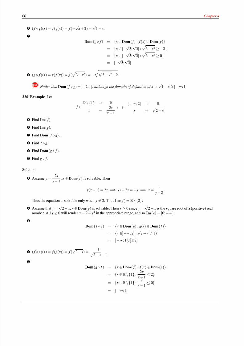
8/8/2019 Pre Calculus I
http://slidepdf.com/reader/full/pre-calculus-i 72/125
66 Chapter 4
( f ◦ g)( x) = f (g( x)) = f (−√ x + 2) =
√1 − x.
Dom(g ◦ f ) = { x ∈ Dom( f ) : f ( x) ∈ Dom(g)}= { x ∈ [−
√3;
√3] :
3 − x2 ≥ −2}
=
{ x
∈[
−
√3;
√3] : 3 −
x2
≥0
}= [−√3;√3]
(g ◦ f )( x) = g( f ( x)) = g(
3 − x2) = −
3− x2 + 2.
! Notice that Dom( f ◦ g) = [−2; 1] , although the domain of definition of x→ √1 − x is ]−∞; 1].
326 Example Let
f :R\{1} → R
x → 2 x
x − 1
, g :] −∞; 2] → R
x → √2− x
Find Im ( f ).
Find Im (g).
Find Dom( f ◦ g).
Find f ◦ g.
Find Dom(g ◦ f ).
Find g ◦ f .
Solution:
Assume y =
2 x
x − 1 , x ∈ Dom( f ) is solvable. Then
y( x − 1) = 2 x =⇒ yx − 2 x = + y =⇒ x =y
y− 2.
Thus the equation is solvable only when y = 2. Thus Im ( f ) = R\{2}.
Assume that y =√
2 − x, x ∈ Dom(g) is solvable. Then y ≥ 0 since y =√
2 − x is the square root of a (positive) real
number. All y ≥ 0 will render x = 2 − y2 in the appropriate range, and so Im (g) = [0; +∞[.
Dom( f ◦ g) = { x ∈ Dom(g) : g( x) ∈ Dom( f )}= { x ∈]−∞; 2] :
√2 − x = 1}
= ]−∞; 1[∪]1; 2]
( f ◦ g)( x) = f (g( x)) = f (√
2 − x) =1√
2 − x − 1.
Dom(g ◦ f ) = { x ∈ Dom( f ) : f ( x) ∈ Dom(g)}= { x ∈ R\{1} :
2 x
x − 1≤ 2}
= { x ∈ R\{1} :2
x − 1≤ 0}
= ] −∞; 1[
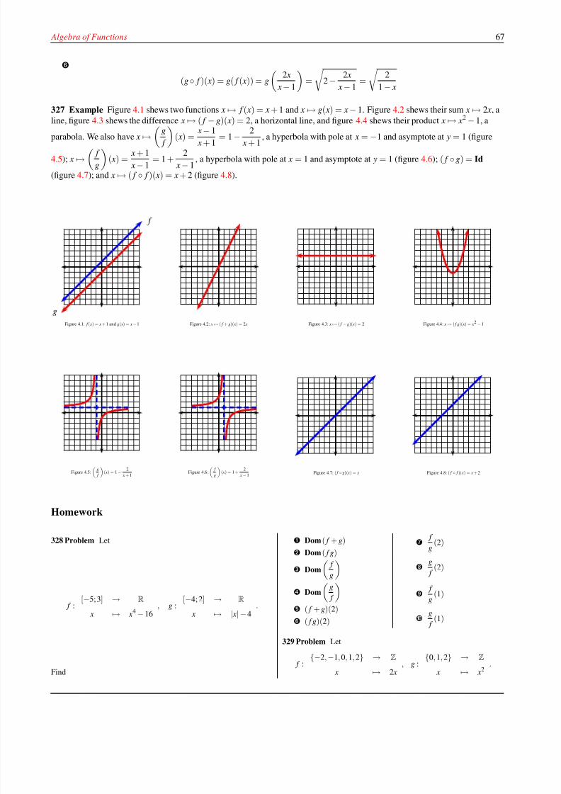
8/8/2019 Pre Calculus I
http://slidepdf.com/reader/full/pre-calculus-i 73/125
Algebra of Functions 67
(g ◦ f )( x) = g( f ( x)) = g
2 x
x − 1
=
2 − 2 x
x − 1=
2
1 − x
327 Example Figure 4.1 shews two functions x → f ( x) = x + 1 and x → g( x) = x − 1. Figure 4.2 shews their sum x → 2 x, a
line, figure 4.3 shews the difference x → ( f − g)( x) = 2, a horizontal line, and figure 4.4 shews their product x → x2 − 1, a
parabola. We also have x → g
f ( x) =
x
−1
x + 1 = 1 −2
x + 1 , a hyperbola with pole at x = −1 and asymptote at y = 1 (figure
4.5); x →
f
g
( x) =
x + 1
x − 1= 1 +
2
x − 1, a hyperbola with pole at x = 1 and asymptote at y = 1 (figure 4.6); ( f ◦ g) = Id
(figure 4.7); and x → ( f ◦ f )( x) = x + 2 (figure 4.8).
f
g
Figure 4.1: f ( x) = x + 1 and g( x) = x −1 Figure 4.2: x → ( f + g)( x) = 2 x Figure 4.3: x → ( f −g)( x) = 2 Figure 4.4: x → ( f g)( x) = x2 −1
Figure 4.5:
g
f
( x) = 1 − 2
x + 1Figure 4.6:
f
g
( x) = 1 +
2
x − 1Figure 4.7: ( f ◦ g)( x) = x Figure 4.8: ( f ◦ f )( x) = x + 2
Homework
328 Problem Let
f :[−5; 3] → R
x → x4 − 16, g :
[−4; 2] → R
x → | x|−4.
Find
Dom ( f + g)
Dom ( f g)
Dom
f
g
Dom
g
f
( f + g)(2)
( f g)(2)
f
g
(2)
g
f (2)
f
g(1)
g
f (1)
329 Problem Let
f :{−2,−1, 0, 1, 2} → Z
x → 2 x, g :
{0, 1, 2} → Z
x → x2.
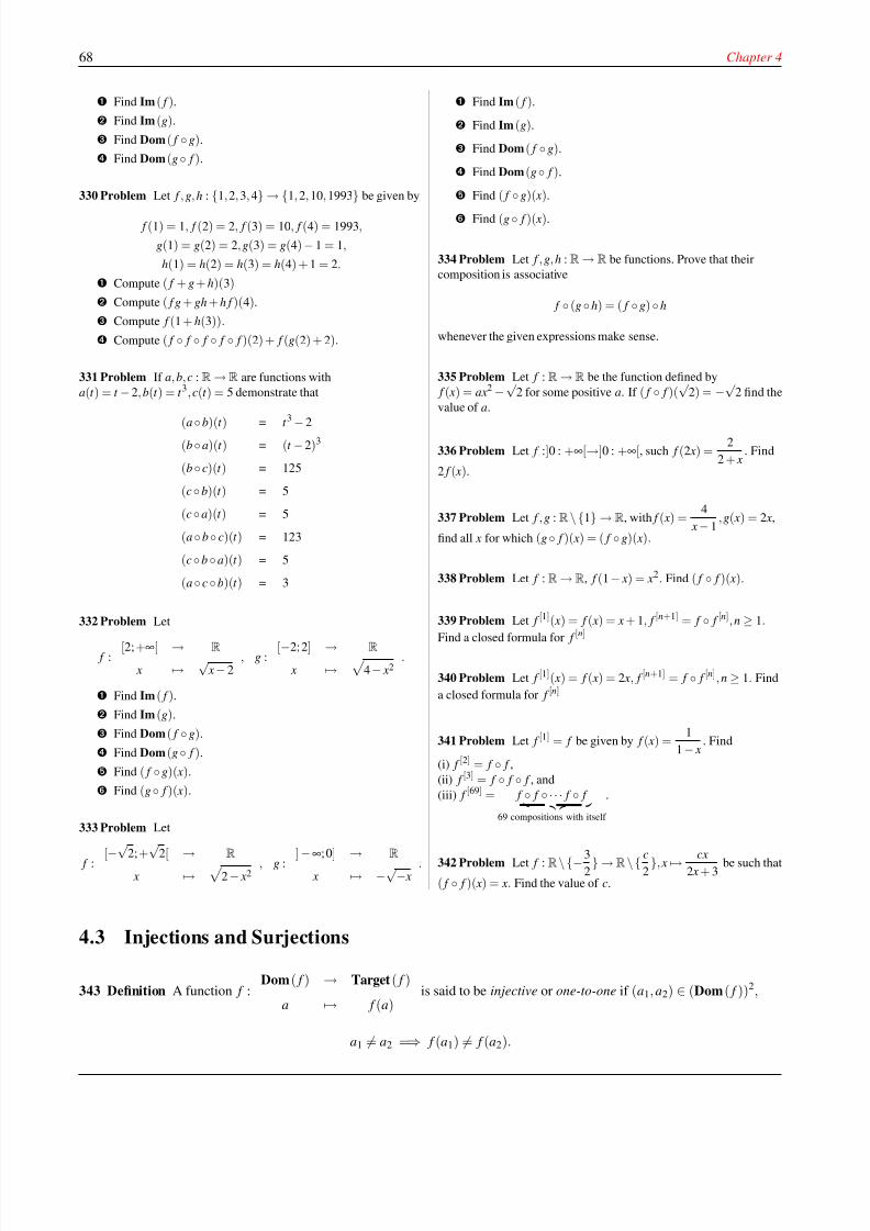
8/8/2019 Pre Calculus I
http://slidepdf.com/reader/full/pre-calculus-i 74/125
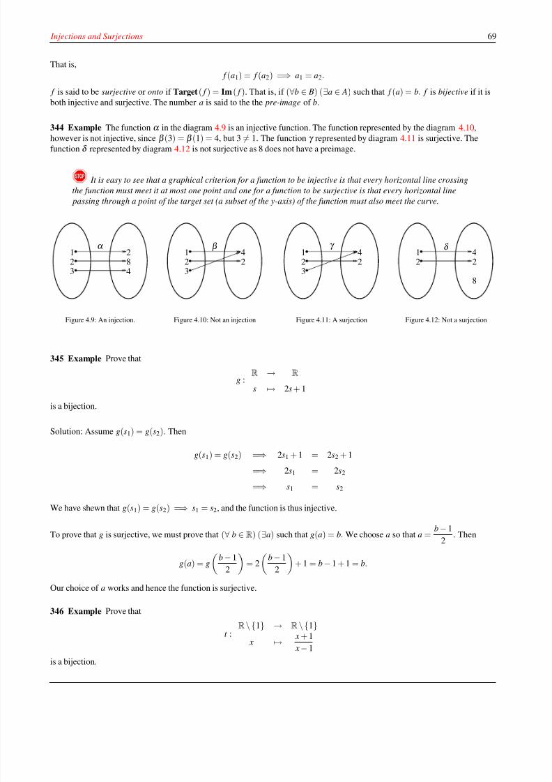
8/8/2019 Pre Calculus I
http://slidepdf.com/reader/full/pre-calculus-i 75/125
Injections and Surjections 69
That is,
f (a1) = f (a2) =⇒ a1 = a2.
f is said to be surjective or onto if Target ( f ) = Im ( f ). That is, if (∀b ∈ B) (∃a ∈ A) such that f (a) = b. f is bijective if it is
both injective and surjective. The number a is said to the the pre-image of b.
344 Example The function α in the diagram 4.9 is an injective function. The function represented by the diagram 4.10,
however is not injective, since β (3) = β (1) = 4, but 3 = 1. The function γ represented by diagram 4.11 is surjective. Thefunction δ represented by diagram 4.12 is not surjective as 8 does not have a preimage.
! It is easy to see that a graphical criterion for a function to be injective is that every horizontal line crossing
the function must meet it at most one point and one for a function to be surjective is that every horizontal line
passing through a point of the target set (a subset of the y-axis) of the function must also meet the curve.
α 1 22 8
3 4
Figure 4.9: An injection.
β
2 21 4
3
Figure 4.10: Not an injection
21
3
24
γ
Figure 4.11: A surjection
8
δ
2 21 4
Figure 4.12: Not a surjection
345 Example Prove that
g :R → R
s → 2s + 1
is a bijection.
Solution: Assume g(s1) = g(s2). Then
g(s1) = g(s2) =⇒ 2s1 + 1 = 2s2 + 1
=⇒ 2s1 = 2s2
=⇒ s1 = s2
We have shewn that g(s1) = g(s2) =⇒ s1 = s2, and the function is thus injective.
To prove that g is surjective, we must prove that (∀
b
∈R) (
∃a) such that g(a) = b. We choose a so that a =
b − 1
2
. Then
g(a) = g
b − 1
2
= 2
b − 1
2
+ 1 = b − 1 + 1 = b.
Our choice of a works and hence the function is surjective.
346 Example Prove that
t :R\{1} → R\{1}
x → x + 1
x − 1
is a bijection.
8/8/2019 Pre Calculus I
http://slidepdf.com/reader/full/pre-calculus-i 76/125
70 Chapter 4
Solution: Assume t (a) = t (b). Then
t (a) = t (b) =⇒ a + 1
a − 1=
b + 1
b − 1
=⇒ (a + 1)(b − 1) = (b + 1)(a − 1)
=⇒ ab − a + b − 1 = ab− b + a − 1
=⇒ 2a = 2b
=⇒ a = b
We have proved that t (a) = t (b) =⇒ a = b, which shews that t is injective.
To prove that t is surjective, we must be able to find a solution a with t (a) = y for y = 1. But
t (a) = y ⇐⇒ a + 1
a − 1= y ⇐⇒ ya− y = a + 1 ⇐⇒ ya − a = 1 + y ⇐⇒ a =
1 + y
1 − y.
This last expression makes sense for y = 1 and thus t is surjective.
347 Example Prove that
h :R
→R
x → x3
is a bijection.
Solution: Assume h(b) = h(a). Then
h(a) = h(b) =⇒ a3 = b3
=⇒ a3 − b3 = 0
=⇒ (a − b)(a2 + ab + b2) = 0
Now,
b
2
+ ab + a
2
= b +
a
22
+
3a2
4 .
This shews that b2 + ab + a2 is positive unless both a and b are zero. Hence b − a = 0 in all cases. We have shewn that
h(b) = h(a) =⇒ b = a, and the function is thus injective.
To prove that h is surjective, we must prove that (∀ b ∈ R) (∃a) such that h(a) = b. We choose a so that a = b1/3. Then
h(a) = h(b1/3) = (b1/3)3 = b.
Our choice of a works and hence the function is surjective.
348 Example Observe that
h :R → [0; +∞[
w → w
2
is not injective. For h(−2) = h(2) = 4 but −2 = 2. The graph of h is a full parabola opening up and in fact, most vertical lines
crossing h meet the parabola at two points.
349 Example If we however restrict h in example 348 to the positive reals, as
j :[0; +∞[ → [0; +∞[
w → w2
then j is injective. For, it is only the right half of a parabola opening up. We can prove this analytically as follows. Clearly if
j(s) = 0 then s = 0. Assume now that j(a) = j(b) with a, b positive. Then a2 = b2 which is to say (a − b)(a + b) = 0. Since
a, b are positive real numbers, a + b > 0. Therefore a − b = 0 which is to say a = b.
8/8/2019 Pre Calculus I
http://slidepdf.com/reader/full/pre-calculus-i 77/125
Inversion 71
350 Example Prove that f :R\{1} → R
x → x1/3
x1/3 − 1
is injective but not surjective.
Solution: We have
f (a) = f (b) =⇒
a1/3
a1/3 − 1=
b1/3
b1/3 − 1=⇒ a1/3b1/3 − a1/3 = a1/3b1/3 − b1/3
=⇒ −a1/3 = −b1/3
=⇒ a = b,
whence f is injective. To prove that f is not surjective assume that f ( x) = b, b ∈ R. Then
f ( x) = b =⇒ x1/3
x1/3 − 1= b =⇒ x =
b3
(b − 1)3.
The expression for x is not a real number when b = 1, and so there is no real x such that f ( x) = 1.
Homework
351 Problem Prove that h :R→R given by h(s) = 3− s is a
bijection.
352 Problem Prove that g :R→R given by g( x) = x1/3 is a
bijection.
353 Problem Prove that f :R\{−1} →R\{1} given by
f ( x) =x −1
x + 1is a bijection.
354 Problem Prove that f :R\{1} → R\{2}
x → 2 x
x + 1
is surjective
but that g :R\{1} → R
x → 2 x
x + 1
is not surjective.
355 Problem Classify each of the following as injective, surjective,
bijective or neither.
f :R→R, x → x4
f :R→ {1}, x → 1
f : {1, 2,3} → {a, b}, f (1) = f (2) = a, f (3) = b
f : [0; +∞[→R, x → x3
f :R→R, x → | x| f : [0; +∞[→R, x → −| x| f :R→ [0; +∞[, x → | x| f : [0; +∞[→ [0; +∞[, x → x4
356 Problem Let f : E → F , g : F → G be two functions. Prove that
if g◦ f is surjective then g is surjective.
357 Problem Let f : E → F , g : F → G be two functions. Prove that
if g◦ f is injective then f is injective.
4.4 Inversion
358 Definition Let A × B ⊆ R
2
. A function F : A → B is said to be invertible if there exists a function F −1
(called the inverseof F ) such that F ◦ F −1 = Id B and F −1 ◦ F = Id A. Here Id S is the identity on the set S function with rule Id S( x) = x.
Consider the functions u : {a, b, c} → { x, y, z} and v : { x, y, z} → {a, b, c} as given by diagram 4.13. It is clear the v undoes
whatever u does. Furthermore, we observe that u and v are bijections and that the domain of u is the image of v and vice-versa.
This example motivates the following theorem.
359 Theorem A function f : A → B is invertible if and only if it is a bijection.
Proof: Assume first that f is invertible. Then there is a function f −1 : B → A such that
f ◦ f −1 = Id B and f −1 ◦ f = Id A. (4.2)
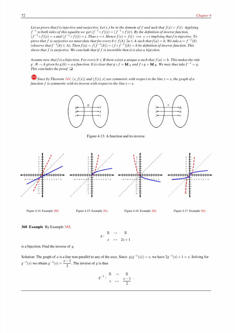
8/8/2019 Pre Calculus I
http://slidepdf.com/reader/full/pre-calculus-i 78/125
8/8/2019 Pre Calculus I
http://slidepdf.com/reader/full/pre-calculus-i 79/125
Inversion 73
The graphs of g (dashed), g−1 (solid) and the identity function (dotted) appear in figure 4.14.
361 Example
f :[0; +∞[ → [0; +∞[
x → x2
has inverse
f −1 :[0; +∞[ → [0; +∞[
x → √ x
.
The graph of f (dashed), f −1 (solid) and the line y = x (dotted) appear in figure 4.15.
362 Example
g :] −∞; 0] → [0; +∞[
x → x2
has inverse
g−1
:
[0; +∞[
→]
−∞; 0]
x → −√ x
.
g−1( x) = −√ x. The graphs of g (dashed), g−1 (solid) and the line y = x appear in figure 4.16.
363 Example Let
b :R → R
x → x3
Find the inverse of b.
Solution: Since b(b−1( x)) = x, we have (b−1( x))3 = x. Solving for b−1( x) we obtain b−1( x) = x1/3. The inverse of b is
b−1 :R → R
x → x1/3.
We will see in Theorem 375 how to graph b. The graph of b and its inverse appear in figure 4.17.
364 Example Consider the rule
f ( x) =1√
x4
−1
.
Find the natural domain of f .
Find the inverse assignment rule f −1.
Find the image of the natural domain of f and find the natural domain of f −1.
Conclude.
Solution:
The expression under the square root must be positive. Hence x4 − 1 > 0 and the natural domain is ]−∞;−1[∪]1; +∞].Since f (− x) = f ( x), f is not injective in this natural domain, so in order to find an inverse, we must restrict the domain
to where f is injective.
8/8/2019 Pre Calculus I
http://slidepdf.com/reader/full/pre-calculus-i 80/125
74 Chapter 4
Put
y =1√
x4 − 1.
Observe that y > 0. Now exchange x and y and solve for y:
x =1
y4
−1
=⇒ x2( y4 − 1) = 1 =⇒ y4 =x2 + 1
x2.
Since y > 0 we choose the plus sign and so
y =4
x2 + 1
x2.
Hence
f −1( x) =4
x2 + 1
x2.
The expression for f −1( x) is undefined when x = 0 (notice that it is always positive). Hence the natural domain of f −1
is R\{0}. The image of the natural domain of f is, on the other hand, ]0; +∞[.
The function
f :]1; +∞[ → ]0; +∞[
x → 1√ x4 − 1
is a bijection with inverse
f −1 :
]0; +∞[ → ]1; +∞[
x →
x2 + 1
x2
.
Homework
365 Problem Let
c :R\{−2} → R\{1}
x → x
x + 2
.
Prove that c is bijective and find the inverse of c.
366 Problem Consider the rule
f ( x) =1
3√
x5
−1
.
Find the natural domain of f .
Find the inverse assignment rule f −1.
Find the image of the natural domain of f and the natural
domain of f −1.
Conclude.
367 Problem Verify that the functions below, with their domains
and images, have the claimed inverses.
Assignment Rule Natural Domain Image Inverse
x → √2− x ]−∞; 2] [0; +∞[ x → 2− x2
x → 1√2− x
]−∞; 2[ ]0; +∞[ x → 2− 1
x2
x → 2 + x3
2− x3R\{ 3
√2} R\{−1} x → 3
2 x −2
x + 1
x → 1
x3 −1R\{1} R\{0} x → 3
1 +
1
x
368 Problem Let f , g, h : {1, 2, 3, 4} → {1, 2, 10,1993} be given by
f (1) = 1, f (2) = 2, f (3) = 10, f (4) = 1993, g(1) = g(2) = 2, g(3) =g(4) − 1 = 1, h(1) = h(2) = h(3) = h(4) + 1 = 2.
Is f invertible? Why? If so, what is f −1( f (h(4)))?
Is g one-to-one? Why?
369 Problem Given g :R→R, g( x) = 2 x + 8 and
f :R\{−2} →R\{0}, f ( x) =1
x + 2find (g ◦ f −1)(−2).
370 Problem Let f , g : A → A be invertible. Shew that f ◦ g is
invertible and that ( f ◦ g)−1 = g−1 ◦ f −1.
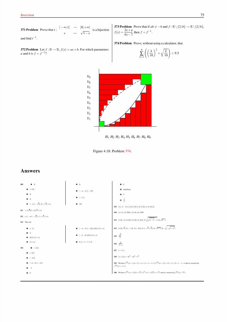
8/8/2019 Pre Calculus I
http://slidepdf.com/reader/full/pre-calculus-i 81/125
8/8/2019 Pre Calculus I
http://slidepdf.com/reader/full/pre-calculus-i 82/125
76 Chapter 4
341 We have (i) f [2] ( x) = ( f ◦ f )( x) = f ( f ( x)) =1
1− 11− x
=x −1
x.
(ii) f [3]( x) = ( f ◦ f ◦ f )( x) = f ( f [2]( x))) = f
x− 1
x
=
1
1− x−1 x
= x.
(iii) Notice that f [4] ( x) = ( f ◦ f [3] )( x) = f ( f [3] ( x)) = f ( x) = f [1] ( x). We see that f is cyclic of period 3, that is,
f [1] = f [14] = f [7] = . . . , f [2] = f [5] = f [8] = . . . , f [3] = f [6] = f [9] = .. .. Hence f [69] ( x) = f [3] ( x) = x.
342 c = −3
354 We must shew that there is a solution x for the equation f ( x) = b, b ∈ R\{2}. Now
f ( x) = b =⇒ 2 x x + 1
= b =⇒ x = b2 −b
.
Thus as long as b = 2 there is x ∈ R with f ( x) = b. Since there is no x such that g( x) = 2 and 2 ∈ Target(g), g is not
surjective.
355 neither, f (−1) = f (1) so not injective. There is no a with f (a) = −1, so not surjective.
surjective, f (1) = f (−1) so not injective.
surjective, not injective.
injective, as proved in text, there is no a with f (a) = −1, so not surjective.
neither, |1| = |− 1| so not injective, there is no a with |a| = −1, so not surjective.
injective, non-surjective since, say, there is no a with −|a| = 1.
surjective, non-injective since, say, |− 1| = |1| but −1 = 1.
bijective.
365 Since c(c−
1( x)) = x, we havec−1( x)
c−1( x)+ 2= x. Solving for c
−1( x) we obtain c
−1( x) =
2 x
1 − x=
−2 +
2
1− x. The
inverse of c is therefore
c−1 :R\{1} → R\{−2}
x → −2 +2
1− x
.
366 We have
The expression under the cubic root must not be 0. Hence x5 = 1 and the natural domain is R\{1}.
Put
y =1
3 x5 −1
.
Now exchange x and y and solve for y:
x =1
3
y5 − 1
=⇒ x3( y5 − 1) = 1 =⇒ y =5
x3 + 1
x3.
Hence
f −1( x) =5
x3 + 1
x3.
As x varies in R\{1}, the expression1
3 x5 −1
assumes all positive and negative values, but it is never 0.
Thus Im( f ) = R\{0}. The expression for f −1( x) is undefined when x = 0. Hence the natural domain of f −1
is R\{0}.
The function
f :
R\{1} → R\{0} x → 1
3 x5 − 1
is a bijection with inverse
f −1 :
R\{0} → R\{1}
x → 5
x3 + 1
x3
.
368 1) Yes, f is a bijection. f −1( f (h(4))) = h(4) = 1, 2) No
369 3
371 t −1 :[0; +∞[ → ]−∞;1 ]
x → 1 − x2
372 Either a = 1, b = 0 or a = −1 and b arbitrary.
374 The inverse of
f :[0; +∞[ → [0; +∞[
x
→x2
is
f −1 :[0; +∞[ → [0; +∞[
x → √ x
.
In diagram 4.18, each rectangle V k has its lower left corner at (0,k
10), base
k
10and height
1
10. Each rectangle H k has
lower left corner at (k
10, 0), base
1
10and height (
k
10)2 . The collective area of these rectangles is
1
10
1
10
2+
1
10+
2
10
2+
2
10+
3
10
2+
3
10+ ·· ·+
9
10
2+
9
10
Since these grey rectangles do not intersect with the green squares on the corners, their collective area is less than the area
of the unit square minus these smaller squares: 1 − 1
100− 4
100=
95
100. We thus conclude that
1
10
1
10
2+
1
10+
2
10
2+
2
10+
3
10
2+
3
10+ ·· · +
9
10
2+
9
10
<
95
100.
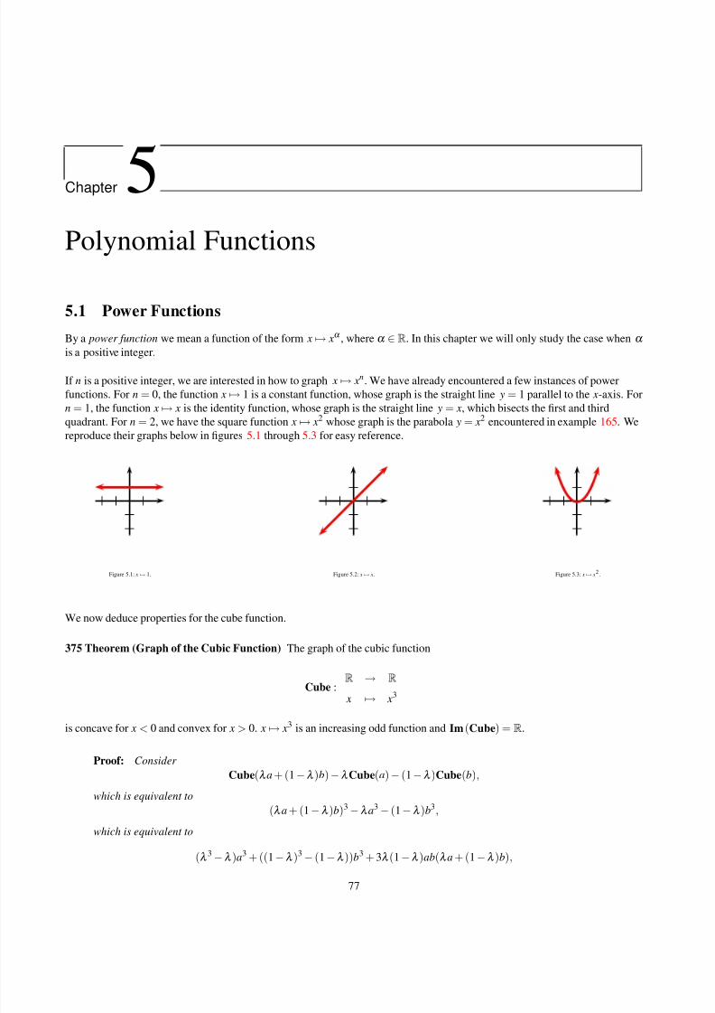
8/8/2019 Pre Calculus I
http://slidepdf.com/reader/full/pre-calculus-i 83/125
Chapter
5Polynomial Functions
5.1 Power Functions
By a power function we mean a function of the form x
→ xα , where α
∈R. In this chapter we will only study the case when α
is a positive integer.
If n is a positive integer, we are interested in how to graph x → xn. We have already encountered a few instances of power
functions. For n = 0, the function x → 1 is a constant function, whose graph is the straight line y = 1 parallel to the x-axis. For
n = 1, the function x → x is the identity function, whose graph is the straight line y = x, which bisects the first and third
quadrant. For n = 2, we have the square function x → x2 whose graph is the parabola y = x2 encountered in example 165. We
reproduce their graphs below in figures 5.1 through 5.3 for easy reference.
Figure 5.1: x → 1. Figure 5.2: x → x. Figure 5.3: x → x2 .
We now deduce properties for the cube function.
375 Theorem (Graph of the Cubic Function) The graph of the cubic function
Cube :R → R
x → x3
is concave for x < 0 and convex for x > 0. x → x3 is an increasing odd function and Im (Cube) = R.
Proof: Consider
Cube(λ a + (1 −λ )b)−λ Cube(a) − (1 −λ )Cube(b),
which is equivalent to
(λ a + (1 −λ )b)3 −λ a3 − (1 −λ )b3,
which is equivalent to
(λ 3 −λ )a3 + ((1 −λ )3 − (1 −λ ))b3 + 3λ (1 −λ )ab(λ a + (1 −λ )b),
77
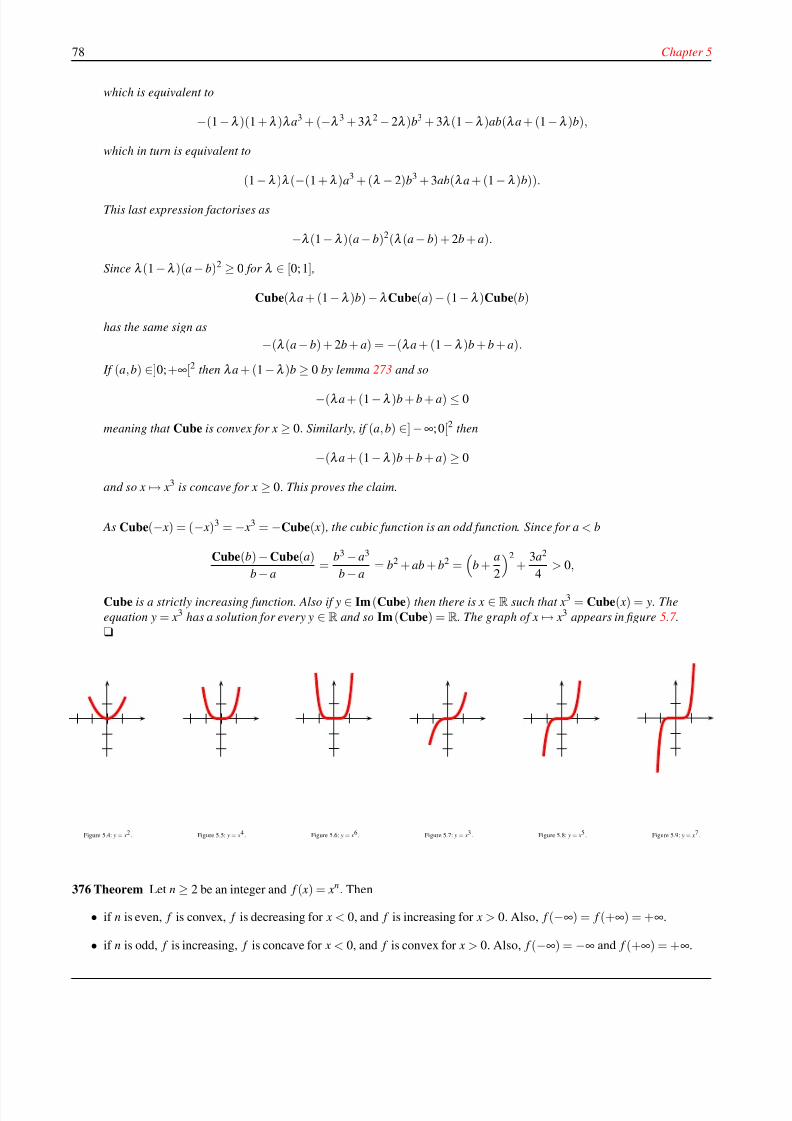
8/8/2019 Pre Calculus I
http://slidepdf.com/reader/full/pre-calculus-i 84/125
78 Chapter 5
which is equivalent to
−(1 −λ )(1 +λ )λ a3 + (−λ 3 + 3λ 2 − 2λ )b3 + 3λ (1 −λ )ab(λ a + (1 −λ )b),
which in turn is equivalent to
(1
−λ )λ (
−(1 +λ )a3 + (λ
−2)b3 + 3ab(λ a + (1
−λ )b)).
This last expression factorises as
−λ (1 −λ )(a − b)2(λ (a − b) + 2b + a).
Since λ (1 −λ )(a − b)2 ≥ 0 for λ ∈ [0; 1] ,
Cube(λ a + (1 −λ )b) −λ Cube(a) − (1 −λ )Cube(b)
has the same sign as
−(λ (a − b) + 2b + a) = −(λ a + (1 −λ )b + b + a).
If (a, b) ∈]0; +∞[2 then λ a + (1 −λ )b ≥ 0 by lemma 273 and so
−(λ a + (1 −λ )b + b + a) ≤ 0
meaning that Cube is convex for x ≥ 0. Similarly, if (a, b) ∈] −∞; 0[2 then
−(λ a + (1 −λ )b + b + a) ≥ 0
and so x → x3 is concave for x ≥ 0. This proves the claim.
As Cube(− x) = (− x)3 = − x3 = −Cube( x) , the cubic function is an odd function. Since for a< b
Cube(b) − Cube(a)
b−
a=
b3 − a3
b−
a= b2 + ab + b2 = b +
a
22
+3a2
4> 0,
Cube is a strictly increasing function. Also if y∈ Im (Cube) then there is x ∈ R such that x3 = Cube( x) = y. The
equation y = x3 has a solution for every y ∈ R and so Im (Cube) = R. The graph of x → x3 appears in figure 5.7 .
u
Figure 5.4: y = x2 . Figure 5.5: y = x4 . Figure 5.6: y = x6 . Figure 5.7: y = x3 . Figure 5.8: y = x5 . Figure 5.9: y = x7 .
376 Theorem Let n ≥ 2 be an integer and f ( x) = xn. Then
• if n is even, f is convex, f is decreasing for x < 0, and f is increasing for x > 0. Also, f (−∞) = f (+∞) = +∞.
• if n is odd, f is increasing, f is concave for x < 0, and f is convex for x > 0. Also, f (−∞) = −∞ and f (+∞) = +∞.
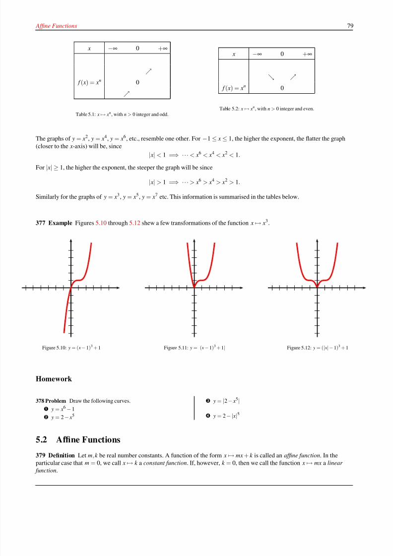
8/8/2019 Pre Calculus I
http://slidepdf.com/reader/full/pre-calculus-i 85/125
Affine Functions 79
x −∞ 0 +∞
ր f ( x) = xn 0
ր
Table 5.1: x → xn, with n > 0 integer and odd.
x −∞ 0 +∞
ց ր f ( x) = xn 0
Table 5.2: x → xn, with n > 0 integer and even.
The graphs of y = x2, y = x4, y = x6, etc., resemble one other. For −1 ≤ x ≤ 1, the higher the exponent, the flatter the graph
(closer to the x-axis) will be, since
| x| < 1 =⇒ ··· < x6 < x4 < x2 < 1.
For | x| ≥ 1, the higher the exponent, the steeper the graph will be since
| x| > 1 =⇒ ··· > x6 > x4 > x2 > 1.
Similarly for the graphs of y = x3, y = x5, y = x7 etc. This information is summarised in the tables below.
377 Example Figures 5.10 through 5.12 shew a few transformations of the function x → x3.
Figure 5.10: y = ( x− 1)3 + 1 Figure 5.11: y = |( x − 1)3 + 1| Figure 5.12: y = (| x|− 1)3 + 1
Homework
378 Problem Draw the following curves.
y = x6 −1
y = 2− x5
y = |2− x5|
y = 2−| x|5
5.2 Affine Functions
379 Definition Let m, k be real number constants. A function of the form x → mx + k is called an affine function. In the
particular case that m = 0, we call x → k a constant function. If, however, k = 0, then we call the function x → mx a linear
function.
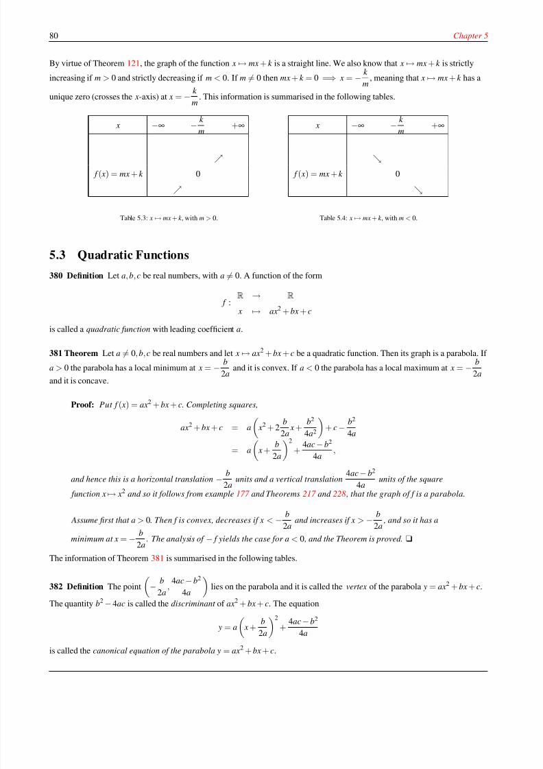
8/8/2019 Pre Calculus I
http://slidepdf.com/reader/full/pre-calculus-i 86/125
80 Chapter 5
By virtue of Theorem 121, the graph of the function x → mx + k is a straight line. We also know that x → mx + k is strictly
increasing if m > 0 and strictly decreasing if m < 0. If m = 0 then mx + k = 0 =⇒ x = − k
m, meaning that x → mx + k has a
unique zero (crosses the x-axis) at x = − k
m. This information is summarised in the following tables.
x
−∞
−k
m
+∞
ր f ( x) = mx + k 0
ր
Table 5.3: x → mx + k , with m > 0.
x
−∞
−k
m
+∞
ց f ( x) = mx + k 0
ց
Table 5.4: x → mx + k , with m < 0.
5.3 Quadratic Functions
380 Definition Let a, b, c be real numbers, with a = 0. A function of the form
f :R → R
x → ax2 + bx + c
is called a quadratic function with leading coefficient a.
381 Theorem Let a = 0, b, c be real numbers and let x → ax2 + bx + c be a quadratic function. Then its graph is a parabola. If
a > 0 the parabola has a local minimum at x = − b
2aand it is convex. If a < 0 the parabola has a local maximum at x = − b
2aand it is concave.
Proof: Put f ( x) = ax2 + bx + c. Completing squares,
ax2 + bx + c = a
x2 + 2
b
2a x +
b2
4a2
+ c − b2
4a
= a
x +
b
2a
2
+4ac − b2
4a,
and hence this is a horizontal translation − b
2aunits and a vertical translation
4ac− b2
4aunits of the square
function x → x2 and so it follows from example 177 and Theorems 217 and 228 , that the graph of f is a parabola.
Assume first that a > 0. Then f is convex, decreases if x < − b
2aand increases if x > − b
2a , and so it has a
minimum at x = − b2a
. The analysis of − f yields the case for a < 0 , and the Theorem is proved. u
The information of Theorem 381 is summarised in the following tables.
382 Definition The point
− b
2a,
4ac − b2
4a
lies on the parabola and it is called the vertex of the parabola y = ax2 + bx + c.
The quantity b2 − 4ac is called the discriminant of ax2 + bx + c. The equation
y = a
x +
b
2a
2
+4ac− b2
4a
is called the canonical equation of the parabola y = ax2 + bx + c.
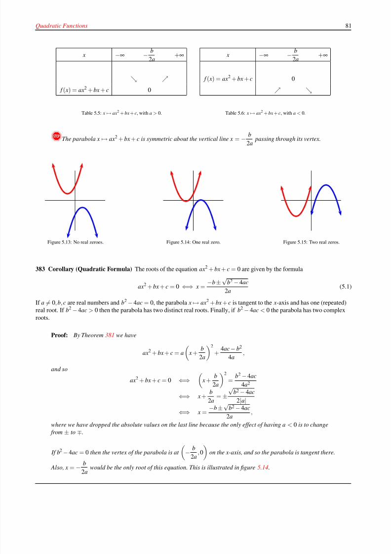
8/8/2019 Pre Calculus I
http://slidepdf.com/reader/full/pre-calculus-i 87/125
Quadratic Functions 81
x −∞ − b
2a+∞
ց ր f ( x) = ax2 + bx + c 0
Table 5.5: x → ax2 + bx + c, with a > 0.
x −∞ − b
2a+∞
f ( x) = ax2 + bx + c 0
ր ց
Table 5.6: x → ax2 + bx + c, with a < 0.
!The parabola x → ax2 + bx + c is symmetric about the vertical line x = − b
2apassing through its vertex.
Figure 5.13: No real zeroes. Figure 5.14: One real zero. Figure 5.15: Two real zeros.
383 Corollary (Quadratic Formula) The roots of the equation ax2 + bx + c = 0 are given by the formula
ax2
+ bx + c = 0 ⇐⇒ x = −b
±
√b2
−4ac
2a (5.1)
If a = 0, b, c are real numbers and b2 − 4ac = 0, the parabola x → ax2 + bx + c is tangent to the x-axis and has one (repeated)
real root. If b2 − 4ac > 0 then the parabola has two distinct real roots. Finally, if b2 − 4ac < 0 the parabola has two complex
roots.
Proof: By Theorem 381 we have
ax2 + bx + c = a
x +
b
2a
2
+4ac− b2
4a,
and so
ax2
+bx
+c
=0
⇐⇒ x+
b
2a2
=
b2
−4ac
4a2
⇐⇒ x +b
2a= ±
√b2 − 4ac
2|a|⇐⇒ x =
−b ±√b2 − 4ac
2a,
where we have dropped the absolute values on the last line because the only effect of having a< 0 is to change
from ± to ∓.
If b2 − 4ac = 0 then the vertex of the parabola is at
− b
2a, 0
on the x-axis, and so the parabola is tangent there.
Also, x = − b
2awould be the only root of this equation. This is illustrated in figure 5.14.
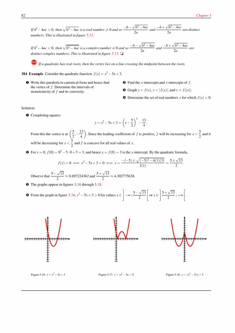
8/8/2019 Pre Calculus I
http://slidepdf.com/reader/full/pre-calculus-i 88/125
82 Chapter 5
If b2 − 4ac > 0 , then
b2 − 4ac is a real number = 0 and so−b −√
b2 − 4ac
2aand
−b +√
b2 − 4ac
2aare distinct
numbers. This is illustrated in figure 5.15.
If b2 − 4ac < 0 , then
b2 − 4ac is a complex number = 0 and so−b −√
b2 − 4ac
2aand
−b +√
b2 − 4ac
2aare
distinct complex numbers. This is illustrated in figure 5.13. u
! If a quadratic has real roots, then the vertex lies on a line crossing the midpoint between the roots.
384 Example Consider the quadratic function f ( x) = x2 − 5 x + 3.
Write this parabola in canonical form and hence find
the vertex of f . Determine the intervals of
monotonicity of f and its convexity.
Find the x-intercepts and y-intercepts of f .
Graph y = f ( x), y = | f ( x)|, and y = f (| x|).
Determine the set of real numbers x for which f ( x) > 0.
Solution:
Completing squares
y = x2 − 5 x + 3 =
x − 5
2
2
− 13
4.
From this the vertex is at
5
2,−13
4
. Since the leading coefficient of f is positive, f will be increasing for x >
5
2and it
will be decreasing for x <5
2and f is concave for all real values of x.
For x = 0, f (0) = 02 − 5 · 0 + 3 = 3, and hence y = f (0) = 3 is the y-intercept. By the quadratic formula,
f ( x) = 0 ⇐⇒ x2 − 5 x + 3 = 0 ⇐⇒ x =−(−5) ±
(−5)2 − 4(1)(3)
2(1)=
5±√13
2.
Observe that 5 −√132
≈ 0.697224362 and 5 +√132
≈ 4.302775638.
The graphs appear in figures 5.16 through 5.18.
From the graph in figure 5.16, x2 − 5 x + 3 > 0 for values x ∈−∞ ;
5−√13
2
or x ∈
5 +
√13
2; +∞
.
Figure 5.16: y = x2 − 5 x + 3 Figure 5.17: y = | x2 − 5 x + 3| Figure 5.18: y = | x|2 − 5| x|+ 3
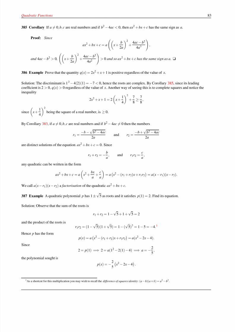
8/8/2019 Pre Calculus I
http://slidepdf.com/reader/full/pre-calculus-i 89/125
Quadratic Functions 83
385 Corollary If a = 0, b, c are real numbers and if b2 − 4ac < 0, then ax2 + bx + c has the same sign as a.
Proof: Since
ax2 + bx + c = a
x +
b
2a
2
+4ac− b2
4a2
,
and 4ac− b2 > 0 , x + b2a2
+ 4ac − b2
4a2 > 0 and so ax2 + bx + c has the same sign as a. u
386 Example Prove that the quantity q( x) = 2 x2 + x + 1 is positive regardless of the value of x.
Solution: The discriminant is 12 − 4(2)(1) = −7 < 0, hence the roots are complex. By Corollary 385, since its leading
coefficient is 2 > 0, q( x) > 0 regardless of the value of x. Another way of seeing this is to complete squares and notice the
inequality
2 x2 + x + 1 = 2
x +
1
4
2
+7
8≥ 7
8,
since x +1
42
being the square of a real number, is
≥0.
By Corollary 383, if a = 0, b, c are real numbers and if b2 − 4ac = 0 then the numbers
r 1 =−b −√
b2 − 4ac
2aand r 2 =
−b +√
b2 − 4ac
2a
are distinct solutions of the equation ax2 + bx + c = 0. Since
r 1 + r 2 = −b
a, and r 1r 2 =
c
a,
any quadratic can be written in the form
ax2 + bx + c = a
x2 + bxa
+ ca
= a
x2 − (r 1 + r 2) x + r 1r 2
= a( x − r 1)( x − r 2).
We call a( x − r 1)( x − r 2) a factorisation of the quadratic ax2 + bx + c.
387 Example A quadratic polynomial p has 1 ±√
5 as roots and it satisfies p(1) = 2. Find its equation.
Solution: Observe that the sum of the roots is
r 1 + r 2 = 1 −√
5 + 1 +√
5 = 2
and the product of the roots is
r 1r 2 = (1
−
√5)(1 +
√5) = 1
−(√
5)2 = 1
−5 =
−4.1
Hence p has the form
p( x) = a x2 − (r 1 + r 2) x + r 1r 2
= a( x2 − 2 x − 4).
Since
2 = p(1) =⇒ 2 = a(12 − 2(1) − 4) =⇒ a = −2
5,
the polynomial sought is
p( x) = −2
5
x2 − 2 x − 4
.
1As a shortcut for this multiplication you may wish to recall the difference of squares identity: (a− b)(a + b) = a2 −b2.
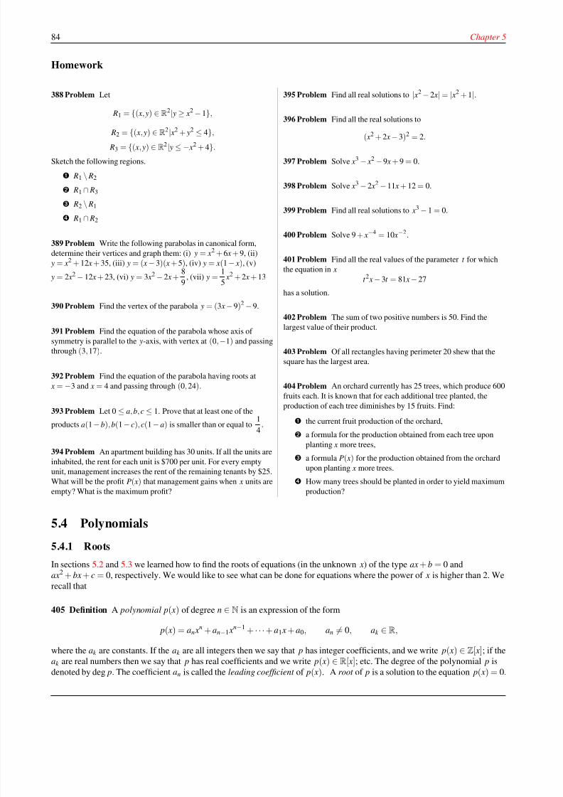
8/8/2019 Pre Calculus I
http://slidepdf.com/reader/full/pre-calculus-i 90/125
84 Chapter 5
Homework
388 Problem Let
R1 = {( x, y) ∈R2| y ≥ x2 −1},
R2 ={
( x, y)∈R2
| x2 + y2
≤4}
,
R3 = {( x, y) ∈ R2| y ≤ − x2 + 4}.
Sketch the following regions.
R1 \ R2
R1 ∩ R3
R2 \ R1
R1 ∩ R2
389 Problem Write the following parabolas in canonical form,
determine their vertices and graph them: (i) y = x2 + 6 x + 9, (ii)
y = x2 + 12 x + 35, (iii) y = ( x − 3)( x + 5), (iv) y = x(1− x), (v)
y = 2 x2 − 12 x + 23, (vi) y = 3 x2 − 2 x +8
9 , (vii) y =1
5 x2 + 2 x + 13
390 Problem Find the vertex of the parabola y = (3 x− 9)2 −9.
391 Problem Find the equation of the parabola whose axis of
symmetry is parallel to the y-axis, with vertex at (0,−1) and passing
through (3,17).
392 Problem Find the equation of the parabola having roots at
x = −3 and x = 4 and passing through (0, 24).
393 Problem Let 0 ≤ a, b, c ≤ 1. Prove that at least one of theproducts a(1−b), b(1−c), c(1− a) is smaller than or equal to
1
4.
394 Problem An apartment building has 30 units. If all the units are
inhabited, the rent for each unit is $700 per unit. For every empty
unit, management increases the rent of the remaining tenants by $25.
What will be the profit P( x) that management gains when x units are
empty? What is the maximum profit?
395 Problem Find all real solutions to | x2 − 2 x| = | x2 + 1|.
396 Problem Find all the real solutions to
( x2
+ 2 x −3)2
= 2.
397 Problem Solve x3 − x2 −9 x + 9 = 0.
398 Problem Solve x3 − 2 x2 −11 x + 12 = 0.
399 Problem Find all real solutions to x3 − 1 = 0.
400 Problem Solve 9 + x−4 = 10 x−2.
401 Problem Find all the real values of the parameter t for which
the equation in x
t 2 x − 3t = 81 x− 27
has a solution.
402 Problem The sum of two positive numbers is 50. Find the
largest value of their product.
403 Problem Of all rectangles having perimeter 20 shew that the
square has the largest area.
404 Problem An orchard currently has 25 trees, which produce 600
fruits each. It is known that for each additional tree planted, the
production of each tree diminishes by 15 fruits. Find:
the current fruit production of the orchard,
a formula for the production obtained from each tree upon
planting x more trees,
a formula P( x) for the production obtained from the orchard
upon planting x more trees.
How many trees should be planted in order to yield maximum
production?
5.4 Polynomials
5.4.1 RootsIn sections 5.2 and 5.3 we learned how to find the roots of equations (in the unknown x) of the type ax + b = 0 and
ax2 + bx + c = 0, respectively. We would like to see what can be done for equations where the power of x is higher than 2. We
recall that
405 Definition A polynomial p( x) of degree n ∈ N is an expression of the form
p( x) = an xn + an−1 x
n−1 + · · · + a1 x + a0, an = 0, ak ∈ R,
where the ak are constants. If the ak are all integers then we say that p has integer coefficients, and we write p( x) ∈ Z[ x]; if the
ak are real numbers then we say that p has real coefficients and we write p( x) ∈ R[ x]; etc. The degree of the polynomial p is
denoted by deg p. The coefficient an is called the leading coefficient of p( x). A root of p is a solution to the equation p( x) = 0.
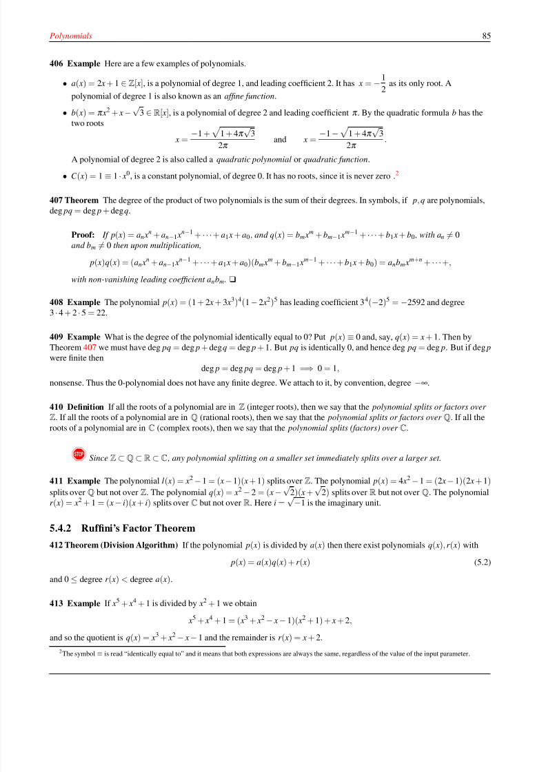
8/8/2019 Pre Calculus I
http://slidepdf.com/reader/full/pre-calculus-i 91/125
Polynomials 85
406 Example Here are a few examples of polynomials.
• a( x) = 2 x + 1 ∈ Z[ x], is a polynomial of degree 1, and leading coefficient 2. It has x = −1
2as its only root. A
polynomial of degree 1 is also known as an affine function.
• b( x) = π x2 + x −√
3 ∈ R[ x], is a polynomial of degree 2 and leading coefficient π . By the quadratic formula b has the
two roots
x = −1 + 1 + 4π √32π
and x = −1 − 1 + 4π √32π
.
A polynomial of degree 2 is also called a quadratic polynomial or quadratic function.
• C ( x) = 1 ≡ 1 · x0, is a constant polynomial, of degree 0. It has no roots, since it is never zero .2
407 Theorem The degree of the product of two polynomials is the sum of their degrees. In symbols, if p, q are polynomials,
deg pq = deg p + degq.
Proof: If p( x) = an xn + an−1 x
n−1 + · · ·+ a1 x + a0, and q( x) = bm xm + bm−1 xm−1 + · · ·+ b1 x + b0 , with an = 0
and bm = 0 then upon multiplication,
p( x
)q
( x
) = (a
n xn
+a
n−1 xn
−1
+ · · · +a
1 x
+a
0)(b
m xm
+b
m−1 xm
−1
+ · · ·+b
1 x
+b
0) =a
nb
m xm+n
+ · · ·+,with non-vanishing leading coefficient anbm. u
408 Example The polynomial p( x) = (1 + 2 x + 3 x3)4(1 − 2 x2)5 has leading coefficient 34(−2)5 = −2592 and degree
3 ·4 + 2 · 5 = 22.
409 Example What is the degree of the polynomial identically equal to 0? Put p( x) ≡ 0 and, say, q( x) = x + 1. Then by
Theorem 407 we must have deg pq = deg p + degq = deg p + 1. But pq is identically 0, and hence deg pq = deg p. But if deg p
were finite then
deg p = deg pq = deg p + 1 =⇒ 0 = 1,
nonsense. Thus the 0-polynomial does not have any finite degree. We attach to it, by convention, degree −∞.
410 Definition If all the roots of a polynomial are in Z (integer roots), then we say that the polynomial splits or factors over
Z. If all the roots of a polynomial are in Q (rational roots), then we say that the polynomial splits or factors over Q. If all the
roots of a polynomial are in C (complex roots), then we say that the polynomial splits (factors) over C.
! Since Z⊂Q⊂ R⊂C , any polynomial splitting on a smaller set immediately splits over a larger set.
411 Example The polynomial l( x) = x2 −1 = ( x−1)( x + 1) splits over Z. The polynomial p( x) = 4 x2 −1 = (2 x− 1)(2 x + 1)
splits over Q but not over Z. The polynomial q( x) = x2 − 2 = ( x −√
2)( x +√
2) splits over R but not over Q. The polynomial
r ( x) = x2 + 1 = ( x − i)( x + i) splits over C but not over R. Here i =√−1 is the imaginary unit.
5.4.2 Ruffini’s Factor Theorem
412 Theorem (Division Algorithm) If the polynomial p( x) is divided by a( x) then there exist polynomials q( x), r ( x) with
p( x) = a( x)q( x) + r ( x) (5.2)
and 0 ≤ degree r ( x) < degree a( x).
413 Example If x5 + x4 + 1 is divided by x2 + 1 we obtain
x5 + x4 + 1 = ( x3 + x2 − x − 1)( x2 + 1) + x + 2,
and so the quotient is q( x) = x3 + x2 − x − 1 and the remainder is r ( x) = x + 2.
2The symbol ≡ is read “identically equal to” and it means that both expressions are always the same, regardless of the value of the input parameter.
8/8/2019 Pre Calculus I
http://slidepdf.com/reader/full/pre-calculus-i 92/125
86 Chapter 5
414 Example Find the remainder when ( x + 3)5 + ( x + 2)8 + (5 x + 9)1997 is divided by x + 2.
Solution: As we are dividing by a polynomial of degree 1, the remainder is a polynomial of degree 0, that is, a constant.
Therefore, there is a polynomial q( x) and a constant r with
( x + 3)5 + ( x + 2)8 + (5 x + 9)1997 = q( x)( x + 2) + r
Letting x = −2 we obtain
(−2 + 3)5 + (−2 + 2)8 + (5(−2) + 9)1997 = q(−2)(−2 + 2) + r = r .
As the sinistral side is 0 we deduce that the remainder r = 0.
415 Example A polynomial leaves remainder −2 upon division by x − 1 and remainder −4 upon division by x + 2. Find the
remainder when this polynomial is divided by x2 + x − 2.
Solution: From the given information, there exist polynomials q1( x), q2( x) with p( x) = q1( x)( x − 1) − 2 and
p( x) = q2( x)( x + 2) − 4. Thus p(1) = −2 and p(−2) = −4. As x2 + x − 2 = ( x − 1)( x + 2) is a polynomial of degree 2, the
remainder r ( x) upon dividing p( x) by x2 + x − 1 is of degree 1 or smaller, that is r ( x) = ax + b for some constants a, b which
we must determine. By the Division Algorithm,
p( x) = q( x)( x2 + x − 1) + ax + b.
Hence
−2 = p(1) = a + b
and
−4 = p(−2) = −2a + b.
From these equations we deduce that a = 2/3, b = −8/3. The remainder sought is
r ( x) =2
3 x − 8
3.
416 Theorem (Ruffini’s Factor Theorem) The polynomial p( x) is divisible by x − a if and only if p(a) = 0. Thus if p is apolynomial of degree n, then p(a) = 0 if and only if p( x) = ( x − a)q( x) for some polynomial q of degree n − 1.
Proof: As x − a is a polynomial of degree 1 , the remainder after diving p( x) by x − a is a polynomial of degree 0 ,
that is, a constant. Therefore
p( x) = q( x)( x − a) + r .
From this we gather that p(a) = q(a)(a − a) + r = r , from where the theorem easily follows. u
417 Example Find the value of a so that the polynomial
t ( x) = x3 − 3ax2 + 2
be divisible by x + 1.
Solution: By Ruffini’s Theorem 416, we must have
0 = t (−1) = (−1)3 − 3a(−1)2 + 2 =⇒ a =1
3.
418 Definition Let a be a root of a polynomial p. We say that a is a root of multiplicity m if p( x) is divisible by ( x − a)m but
not by ( x − a)m+1. This means that p can be written in the form p( x) = ( x − a)mq( x) for some polynomial q with q(a) = 0.
419 Corollary If a polynomial of degree n had any roots at all, then it has at most n roots.
8/8/2019 Pre Calculus I
http://slidepdf.com/reader/full/pre-calculus-i 93/125
Polynomials 87
Proof: If it had at least n+ 1 roots then it would have at least n+ 1 factors of degree 1 and hence degree n + 1 at
least, a contradiction. u
Notice that the above theorem only says that if a polynomial has any roots, then it must have at most its degree number of
roots. It does not say that a polynomial must possess a root. That all polynomials have at least one root is much more difficult
to prove. We will quote the theorem, without a proof.
420 Theorem (Fundamental Theorem of Algebra) A polynomial of degree at least one with complex number coefficientshas at least one complex root.
! The Fundamental Theorem of Algebra implies then that a polynomial of degree n has exactly n roots
(counting multiplicity).
A more useful form of Ruffini’s Theorem is given in the following corollary.
421 Corollary If the polynomial p with integer coefficients,
p( x) = an xn + an−1 x
n−1 + · · ·+ a1 x + a0.
has a rational roots
t ∈Q (here
s
t is assumed to be in lowest terms), then s divides a
0and t divides a
n.
Proof: We are given that
0 = p
s
t
= an
sn
t n
+ an−1
sn−1
t n−1
+ · · ·+ a1
s
t
+ a0.
Clearing denominators,
0 = ansn + an−1sn−1t + · · ·+ a1st n−1 + a0t n.
This last equality implies that
−a0t n = s(ansn−1 + an−1sn−2t + · · ·+ a1t n−1).
Since both sides are integers, and since s and t have no factors in common, then s must divide a0. We also gather
that −ansn = t (an−1sn−1 + · · · + a1st n−2 + a0t n−1),
from where we deduce that t divides an , concluding the proof.u
422 Example Factorise a( x) = x3 − 3 x − 5 x2 + 15 over Z[ x] and over R[ x].
Solution: By Corollary 421, if a( x) has integer roots then they must be in the set {−1, 1,−3, 3,−5, 5}. We test
a(±1), a(±3), a(±5) to see which ones vanish. We find that a(5) = 0. By the Factor Theorem, x − 5 divides a( x). Using long
division,
x2 − 3
x − 5
x3 − 5 x2 − 3 x + 15
− x
3
+ 5 x
2
− 3 x + 15
3 x − 15
0
we find
a( x) = x3 − 3 x − 5 x2 + 15 = ( x − 5)( x2 − 3),
which is the required factorisation over Z[ x]. The factorisation over R[ x] is then
a( x) = x3 − 3 x − 5 x2 + 15 = ( x − 5)( x −√
3)( x +√
3).
8/8/2019 Pre Calculus I
http://slidepdf.com/reader/full/pre-calculus-i 94/125
88 Chapter 5
423 Example Factorise b( x) = x5 − x4 − 4 x + 4 over Z[ x] and over R[ x].
Solution: By Corollary 421, if b( x) has integer roots then they must be in the set {−1, 1,−2, 2,−4, 4}. We quickly see that
b(1) = 0, and so, by the Factor Theorem, x − 1 divides b( x). By long division
x4 − 4
x − 1 x
5
− x
4
− 4 x + 4− x5 + x4
− 4 x + 4
4 x − 4
0
we see that
b( x) = ( x − 1)( x4 − 4) = ( x − 1)( x2 − 2)( x2 + 2),
which is the desired factorisation over Z[ x]. The factorisation over R is seen to be
b( x) = ( x − 1)( x −√
2)( x +√
2)( x2 + 2).
Since the discriminant of x2 + 2 is−
8 < 0, x2 + 2 does not split over R.
424 Lemma Complex roots of a polynomial with real coefficients occur in conjugate pairs, that is, if p is a polynomial with
real coefficients and if u + vi is a root of p, then its conjugate u − vi is also a root for p. Here i =√−1 is the imaginary unit.
Proof: Assume
p( x) = a0 + a1 x + · · · + an xn
and that p(u + vi) = 0. Since the conjugate of a real number is itself, and conjugation is multiplicative (Theorem
463) , we have
0 = 0
= p(u + vi)
= a0 + a1(u + vi) + · · ·+ an(u + vi)n
= a0 + a1(u + vi) + · · ·+ an(u + vi)n
= a0 + a1(u − vi) + · · ·+ an(u − vi)n
= p(u − vi),
whence u − vi is also a root. u
Since the complex pair root u ± vi would give the polynomial with real coefficients
( x − u − vi)( x − u + vi) = x2 − 2ux + (u2 + v2),
we deduce the following theorem.
425 Theorem Any polynomial with real coefficients can be factored in the form
A( x − r 1)m1 ( x − r 2)m2 · · ·( x − r k )mk ( x2 + a1 x + b1)n1 ( x2 + a2 x + b2)n2 · · · ( x2 + al x + bl)nl ,
where each factor is distinct, the mi, lk are positive integers and A, r i, ai, bi are real numbers.
8/8/2019 Pre Calculus I
http://slidepdf.com/reader/full/pre-calculus-i 95/125
Graphs of Polynomials 89
Homework
426 Problem Find the cubic polynomial p having zeroes at
x = −1,2, 3 and satisfying p(1) = −24.
427 Problem How many cubic polynomials with leading coefficient
−2 are there splitting in the set {1, 2,3}?
428 Problem Find the cubic polynomial c having a root of x = 1, a
root of multiplicity 2 at x = −3 and satisfying c(2) = 10.
429 Problem A cubic polynomial p with leading coefficient 1
satisfies p(1) = 1, p(2) = 4, p(3) = 9. Find the value of p(4).
430 Problem The polynomial p( x) has integral coefficients and
p( x) = 7 for four different values of x. Shew that p( x) never equals
14.
431 Problem Find the value of a so that the polynomial
t ( x) = x3 −3ax2 + 12
be divisible by x + 4..
432 Problem Let f ( x) = x4 + x3 + x2 + x + 1. Find the remainder
when f ( x5) is divided by f ( x).
433 Problem If p( x) is a cubic polynomial with
p(1) = 1, p(2) = 2, p(3) = 3, p(4) = 5, find p(6).
434 Problem The polynomial p( x) satisfies p(− x) = − p( x). When
p( x) is divided by x − 3 the remainder is 6. Find the remainder when
p( x) is divided by x2 − 9.
435 Problem Factorise x3 + 3 x2 −4 x + 12 over Z[ x].
436 Problem Factorise 3 x4 + 13 x3 −37 x2 − 117 x + 90 over Z[ x].
437 Problem Find a, b such that the polynomial x3 + 6 x2 + ax + b
be divisible by the polynomial x2 + x −12.
5.5 Graphs of Polynomials
We start with the following theorem, which we will state without proof.
438 Theorem A polynomial function x → p( x) is an everywhere continuous function.
439 Theorem Let p( x) = an xn + an−1 x
n−1 + · · · + a1 x + a0 an = 0, be a polynomial with real number coefficients. Then
p(
−∞) = (signum(an))(
−1)n∞, p(+∞) = (signum(an))∞.
Thus a polynomial of odd degree will have opposite signs for values of large magnitude and different sign, and a polynomial
of even degree will have the same sign for values of large magnitude and different sign.
Proof: If x = 0 then
p( x) = an xn + an−1 x
n−1 + · · ·+ a1 x + a0 = an xn
1 +an−1
x+ · · ·+
a1
xn−1+
a0
xn
∼ an x
n,
since as x → ±∞ , the quantity in parenthesis tends to 1 and so the eventual sign of p( x) is determined by an xn ,
which gives the result. u
440 Corollary A polynomial of odd degree with real number coefficients always has a real root.
Proof: Since a polynomial of odd degree eventually changes sign, since it is continuous, the corollary follows
from Bolzano’s Intermediate Value Theorem 268. u
We now consider polynomials with real number coefficients and that split in R. Such polynomials have the form
p( x) = a( x − r 1)m1 ( x − r 2)m2 · · ·( x − r k )mk ,
where a = 0 and the r i are real numbers and the mi ≥ 1 are integers. Graphing such polynomials will be achieved by referring
to the following theorem.
441 Theorem Let a = 0 and the r i are real numbers and the mi be positive integers. Then the graph of the polynomial
p( x) = a( x − r 1)m1 ( x − r 2)m2 · · ·( x − r k )mk ,
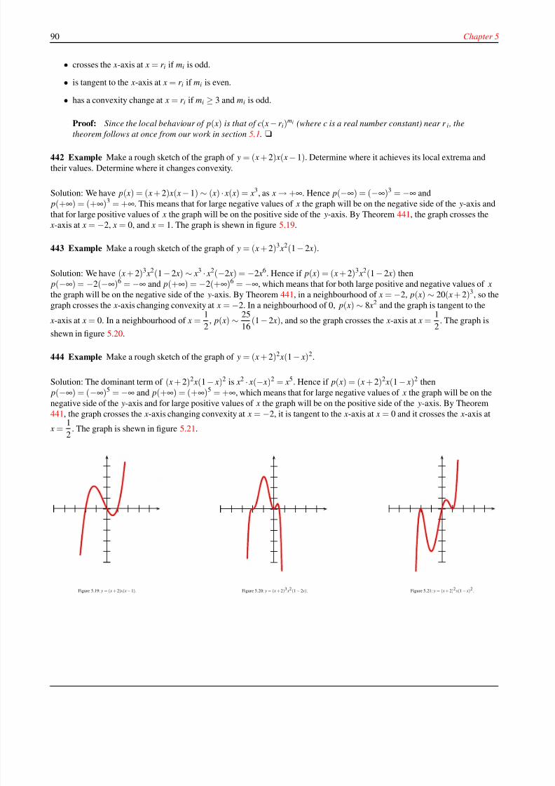
8/8/2019 Pre Calculus I
http://slidepdf.com/reader/full/pre-calculus-i 96/125
90 Chapter 5
• crosses the x-axis at x = r i if mi is odd.
• is tangent to the x-axis at x = r i if mi is even.
• has a convexity change at x = r i if mi ≥ 3 and mi is odd.
Proof: Since the local behaviour of p( x) is that of c( x − r i)mi (where c is a real number constant) near r i , the
theorem follows at once from our work in section 5.1. u
442 Example Make a rough sketch of the graph of y = ( x + 2) x( x − 1). Determine where it achieves its local extrema and
their values. Determine where it changes convexity.
Solution: We have p( x) = ( x + 2) x( x − 1) ∼ ( x) · x( x) = x3, as x → +∞. Hence p(−∞) = (−∞)3 = −∞ and
p(+∞) = (+∞)3 = +∞. This means that for large negative values of x the graph will be on the negative side of the y-axis and
that for large positive values of x the graph will be on the positive side of the y-axis. By Theorem 441, the graph crosses the
x-axis at x = −2, x = 0, and x = 1. The graph is shewn in figure 5.19.
443 Example Make a rough sketch of the graph of y = ( x + 2)3 x2(1 − 2 x).
Solution: We have ( x + 2)3 x2(1 − 2 x) ∼ x3 · x2(−2 x) = −2 x6. Hence if p( x) = ( x + 2)3 x2(1 − 2 x) then p(−∞) = −2(−∞)6 = −∞ and p(+∞) = −2(+∞)6 = −∞, which means that for both large positive and negative values of x
the graph will be on the negative side of the y-axis. By Theorem 441, in a neighbourhood of x = −2, p( x) ∼ 20( x + 2)3, so the
graph crosses the x-axis changing convexity at x = −2. In a neighbourhood of 0, p( x) ∼ 8 x2 and the graph is tangent to the
x-axis at x = 0. In a neighbourhood of x =1
2, p( x) ∼ 25
16(1 − 2 x), and so the graph crosses the x-axis at x =
1
2. The graph is
shewn in figure 5.20.
444 Example Make a rough sketch of the graph of y = ( x + 2)2 x(1 − x)2.
Solution: The dominant term of ( x + 2)2 x(1 − x)2 is x2 · x(− x)2 = x5. Hence if p( x) = ( x + 2)2 x(1 − x)2 then
p(−∞) = (−∞)5 = −∞ and p(+∞) = (+∞)5 = +∞, which means that for large negative values of x the graph will be on the
negative side of the y-axis and for large positive values of x the graph will be on the positive side of the y-axis. By Theorem
441, the graph crosses the x-axis changing convexity at x = −2, it is tangent to the x-axis at x = 0 and it crosses the x-axis at
x =1
2. The graph is shewn in figure 5.21.
Figure 5.19: y = ( x + 2) x( x− 1). Figure 5.20: y = ( x + 2)3 x2(1− 2 x). Figure 5.21: y = ( x + 2)2 x(1− x)2 .
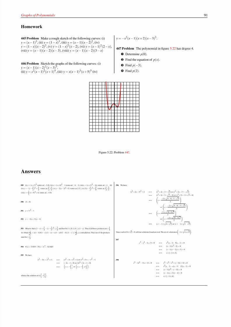
8/8/2019 Pre Calculus I
http://slidepdf.com/reader/full/pre-calculus-i 97/125
Graphs of Polynomials 91
Homework
445 Problem Make a rough sketch of the following curves: (i)
y = ( x− 1)3, (ii) y = (1− x)3, (iii) y = ( x − 1)( x −2)2, (iv)
y = (1− x)( x −2)2, (v) y = (1− x)2( x− 2), (vi) y = ( x −1)2(2− x),
(vii) y = ( x −1)( x− 2)( x −3), (viii) y = ( x − 1)( x −2)(3 − x)
446 Problem Sketch the graphs of the following curves: (i)
y = ( x− 1)( x −2)2( x −3)3,
(ii) y = x2( x− 1)2( x + 1)4, (iii) y = x( x −1)3( x + 5)5 (iv)
y = − x2( x− 1)( x + 2)( x− 3)3.
447 Problem The polynomial in figure 5.22 has degree 4.
Determine p(0).
Find the equation of p( x).
Find p(−3).
Find p(2).
Figure 5.22: Problem 447.
Answers
389 (i) y = ( x + 3)2 vertex at (−3, 0), (ii) y = ( x + 6)2 −1 vertex at (−6,−1), (iii) y = ( x + 1)2 − 16, vertex at (−1,−16)
(iv) y = −( x − 1
2)2 +
1
4, vertex at (
1
2,
1
4) (v) y = 2( x− 3)2 + 5, vertex at (3, 5), (vi) 3( x− 1
3)2 +
5
9, vertex at (
1
3,
5
9)
(vii) y =1
5( x + 5)2 + 8, vertex at (−5, 8)
390 (3,−9)
391 y = 2 x2 − 1
392 y = −2( x + 3)( x− 4)
393 Observe that x(1 − x) =1
4−( x− 1
2)2 ≤ 1
4and that for x ∈ [0, 1], 0 ≤ x(1 − x). Thus if all these products are >
1
4
we obtain1
43< a(1 −b)b(1− c)c(1− a) = a(1− a)b(1 −b)c(1− c) ≤ 1
43, a contradiction. Thus one of the products
must be ≤ 1
4.
394 P( x) = 21025− 25( x −1)2 ; $21025
395 We have
| x2 −2 x| = | x2 + 1| ⇐⇒ ( x2 − 2 x = x2 + 1) or ( x2 + 2 x = − x2 − 1)
⇐⇒ (−2 x − 1 = 0) or (2 x2 + 2 x + 1 = 0)
⇐⇒
x = − 1
2
or
x = − 1
2± i
2
,
whence the solution set is
− 1
2
.
396 We have
( x2 + 2 x −3)2 = 2 ⇐⇒ ( x2 + 2 x − 3 =√
2) or ( x2 + 2 x− 3 = −√
2)
⇐⇒ ( x2 + 2 x − 3−√
2 = 0) or ( x2 + 2 x− 3 +√
2 = 0)
⇐⇒ x =
−2 ±
4 −4(−3 −√2)
2
or
x =
−2±
4− 4(−3 +√
2)
2
⇐⇒
x =−2 ±
16 + 4
√2
2
or
x =
−2±
16 − 4√
2
2
⇐⇒ ( x = −1± 4 +√
2) or ( x = −1± 4 −√
2).
Since each of 4 ±√
2 > 0, all four solutions found are real. The set of solutions is
−1±
4±
√2
.
397
x3 − x2 − 9 x + 9 = 0 ⇐⇒ x2( x− 1) −9( x −1) = 0
⇐⇒ ( x − 1)( x2 − 9) = 0
⇐⇒ ( x − 1)( x− 3)( x + 3) = 0
⇐⇒ x ∈ {−3, 1, 3}.
398
x3 − 2 x2 − 11 x + 12 = 0 ⇐⇒ x3 − x2 − x2 + x− 12 x + 12 = 0
⇐⇒ x2( x− 1) − x( x −1)− 12( x− 1) = 0
⇐⇒ ( x− 1)( x2 − x− 12) = 0
⇐⇒ ( x− 1)( x + 3)( x− 4) = 0
⇐⇒ x ∈ {−3, 1, 4}.
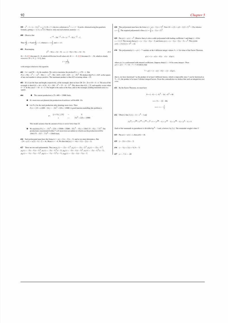
8/8/2019 Pre Calculus I
http://slidepdf.com/reader/full/pre-calculus-i 98/125
92 Chapter 5
399 x3 −1 = ( x− 1)( x2 + x + 1). If x = 1, the two solutions to x2 + x + 1 = 0 can be obtained using the quadratic
formula, getting x = 1/2± i√
3/2. There is only one real solution, namely x = 1.
400 Observe that
x−4 − 10 x−2 + 9 = ( x−2 − 9)( x−2 − 1).
Thus1
x2= 9 and
1
x2= 1, whence x = ± 1
3and x = ±1.
401 Rearranging,
(t 2 − 81) x = 3(t − 9) =⇒ (t −9)(t + 9) x = 3(t −9). (5.3)
If t = 9, (5.3) becomes 0 = 0, which will be true for all values of x. If t = −9, (5.3) becomes 0 = −54, which is clearlynonsense. If t ∈R\{−9, 9}, then
x =3
t + 9
is the unique solution to the equation.
402 Let x and 50− x be the numbers. We seek to maximise the product P( x) = x(50− x). But
P( x) = 50 x− x2 = −( x2 − 50 x) = −( x2 −50 x + 625) + 625 = 625 − ( x −25)2 . We deduce that P( x) ≤ 625, as the square
of any real number is always positive. The maximum product is thus 625 occurring when x = 25.
403 If b, h are the base and height, respectively, of the rectangle, then we have 20 = 2b + 2h or 10 = b + h. The area of the
rectangle is then A(h) = bh = h(10 −h) = 10h− h2 = 25 −(h− 5)2 . This shows that A(h) ≤ 25, and equality occurs when
h = 5. In this case b = 10 − h = 5. The height is the same as the base, and so the rectangle yielding maximum area is a
square.
404 The current production is 25 × 600 = 15000 fruits.
If x more trees are planted, the production of each tree will be 600 − 15 x.
Let P( x) be the total production after planting x more trees. Then
P( x) = (25 + x)(600 −15 x) = −15 x2 + 225 x + 15000. A good function modelling this problem is
P :{ x ∈ N| x ≥ 25} → N
x → −15 x2 + 225 x + 15000.
This model assumes that the amount of trees is never fewer than 25.
We maximise P( x) = −15 x2 + 225 x + 15000 = 15000 − 15( x2 − 15 x) = 15843.75 −15( x −7.5)2. The
production is maximised if either 7 or 8 more trees are added, in which case the production will be
15843.75 − 15(7− 7.5)2 = 15840 fruits.
426 Such polynomial must have the form p( x) = a( x + 1)( x −2)( x −3), and so we must determine a. But
−24 = p(1) = a(2)(−1)(−2) = 4a. Hence a = −6. We thus find p( x) = −6( x + 1)( x− 2)( x− 3).
427 There are ten such polynomials. They are p1( x) = −2( x− 1)3, p2( x) = −2( x− 2)3 , p3( x) = −2( x− 3)3 ,
p4( x) = −2( x− 1)( x −2)2 , p5( x) = −2( x −1)2( x− 2), p6( x) = −2( x −1)( x −3)2 , p7( x) = −2( x −1)2( x −3),
p8( x) = −2( x− 2)( x −3)2 , p9( x) = −2( x −2)2( x− 3), p10( x) = −2( x − 1)( x − 2)( x − 3).
428 This polynomial must have the form c( x) = a( x −1)( x + 3)2 . Now 10 = c(2) = a(2− 1)(2 + 3)2 = 25a, whence
a =2
5. The required polynomial is thus c( x) =
2
5( x− 1)( x + 3)2 .
429 Put g( x) = p( x) − x2. Observe that g is also a cubic polynomial with leading coefficient 1 and that g( x) = 0 for
x = 1, 2, 3. This means that g( x) = ( x −1)( x −2)( x −3) and hence p( x) = ( x− 1)( x −2)( x −3)+ x2 . This yields
p(4) = (3)(2)(1)+ 42 = 22.
430 The polynomial g( x) = p( x)− 7 vanishes at the 4 different integer values a, b, c, d . In virtue of the Factor Theorem,
g( x) = ( x− a)( x− b)( x− c)( x− d )q( x),
where q( x) is a polynomial with integral coefficients. Suppose that p(t ) = 14 for some integer t . Theng(t ) = p(t ) −7 = 14 − 7 = 7. It follows that
7 = g(t ) = (t − a)(t −b)(t − c)(t − d )q(t ),
that is, we have factorised 7 as the product of at least 4 different factors, which is impossible since 7 can be factorised as
7(−1)1, the product of at most 3 distinct integral factors. From this contradiction we deduce that such an integer t does not
exist.
431 By the Factor Theorem, we must have
0 = t (−4) = (−4)3 − 3a(−4)2 + 40
⇐⇒ 0 = −24 − 48a
⇐⇒ a = − 1
2.
432 Observe that f ( x)( x− 1) = x5 −1 and
f ( x5) = x20 + x15 + x10 + x5 + 1 = ( x20 −1)+ ( x15 −1)+ ( x10 −1)+ ( x5 − 1) + 5.
Each of the summands in parentheses is divisible by x5 − 1 and, a fortiori, by f ( x). The remainder sought is thus 5.
433 Put g( x) = p( x) − x, then p(6) = 16.
435 ( x − 2)( x + 2)( x − 3)
436 ( x − 3)( x + 3)( x + 5)(3 x− 2)
437 a = −7, b = −60
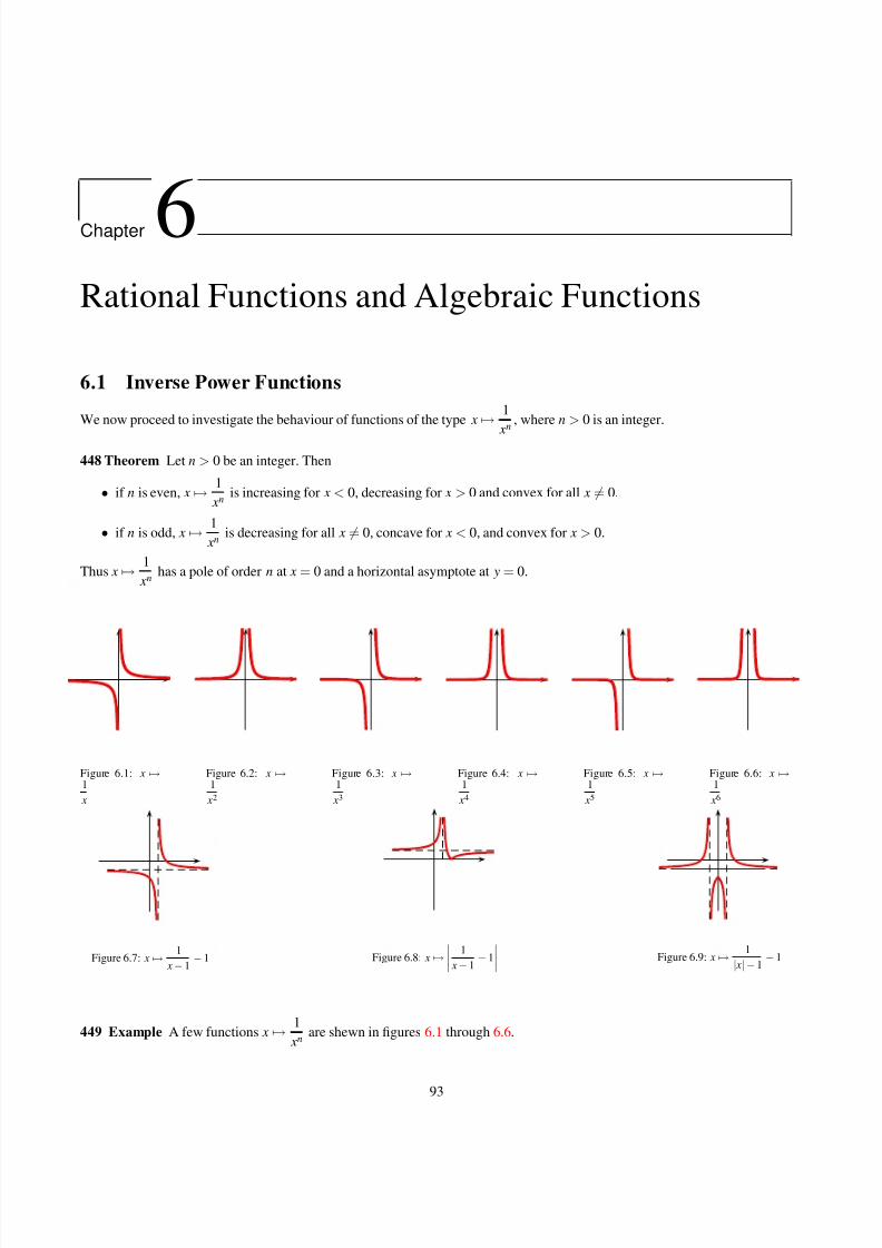
8/8/2019 Pre Calculus I
http://slidepdf.com/reader/full/pre-calculus-i 99/125
Chapter
6Rational Functions and Algebraic Functions
6.1 Inverse Power Functions
We now proceed to investigate the behaviour of functions of the type x
→1
xn
, where n > 0 is an integer.
448 Theorem Let n > 0 be an integer. Then
• if n is even, x → 1
xnis increasing for x < 0, decreasing for x > 0 and convex for all x = 0.
• if n is odd, x → 1
xnis decreasing for all x = 0, concave for x < 0, and convex for x > 0.
Thus x → 1
xnhas a pole of order n at x = 0 and a horizontal asymptote at y = 0.
Figure 6.1: x →1
x
Figure 6.2: x →1
x2
Figure 6.3: x →1
x3
Figure 6.4: x →1
x4
Figure 6.5: x →1
x5
Figure 6.6: x →1
x6
Figure 6.7: x → 1
x− 1− 1 Figure 6.8: x →
1
x− 1− 1
Figure 6.9: x → 1
| x|− 1− 1
449 Example A few functions x → 1
xnare shewn in figures 6.1 through 6.6.
93
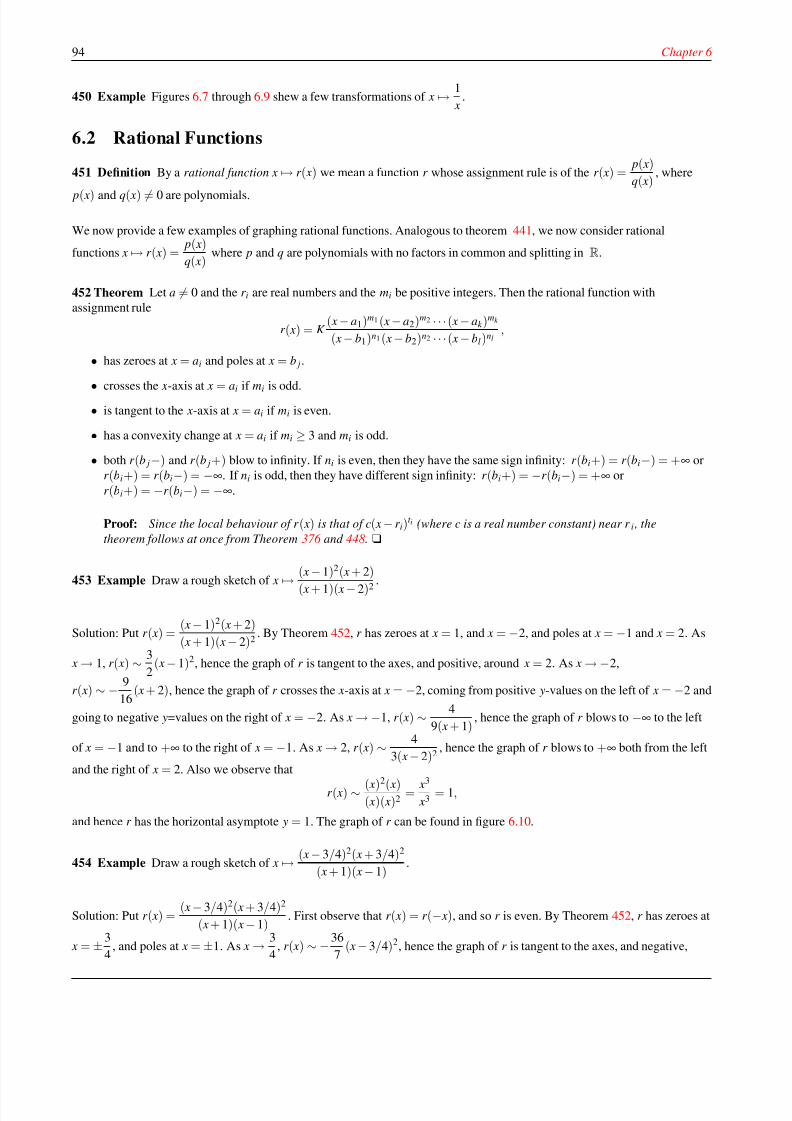
8/8/2019 Pre Calculus I
http://slidepdf.com/reader/full/pre-calculus-i 100/125
94 Chapter 6
450 Example Figures 6.7 through 6.9 shew a few transformations of x → 1
x.
6.2 Rational Functions
451 Definition By a rational function x → r ( x) we mean a function r whose assignment rule is of the r ( x) =p( x)
q( x), where
p( x) and q( x) = 0 are polynomials.
We now provide a few examples of graphing rational functions. Analogous to theorem 441, we now consider rational
functions x → r ( x) =p( x)
q( x)where p and q are polynomials with no factors in common and splitting in R.
452 Theorem Let a = 0 and the r i are real numbers and the mi be positive integers. Then the rational function with
assignment rule
r ( x) = K ( x − a1)m1 ( x − a2)m2 · · · ( x − ak )
mk
( x − b1)n1 ( x − b2)n2 · · ·( x − bl)nl,
• has zeroes at x = ai and poles at x = b j.
• crosses the x-axis at x = ai if mi is odd.
• is tangent to the x-axis at x = ai if mi is even.
• has a convexity change at x = ai if mi ≥ 3 and mi is odd.
• both r (b j−) and r (b j+) blow to infinity. If ni is even, then they have the same sign infinity: r (bi+) = r (bi−) = +∞ or
r (bi+) = r (bi−) = −∞. If ni is odd, then they have different sign infinity: r (bi+) = −r (bi−) = +∞ or
r (bi+) = −r (bi−) = −∞.
Proof: Since the local behaviour of r ( x) is that of c( x − r i)t i (where c is a real number constant) near r i , the
theorem follows at once from Theorem 376 and 448. u
453 Example Draw a rough sketch of x →( x
−1)2( x + 2)
( x + 1)( x − 2)2 .
Solution: Put r ( x) =( x − 1)2( x + 2)
( x + 1)( x − 2)2. By Theorem 452, r has zeroes at x = 1, and x = −2, and poles at x = −1 and x = 2. As
x → 1, r ( x) ∼ 3
2( x − 1)2, hence the graph of r is tangent to the axes, and positive, around x = 2. As x → −2,
r ( x) ∼ − 9
16( x + 2), hence the graph of r crosses the x-axis at x = −2, coming from positive y-values on the left of x = −2 and
going to negative y=values on the right of x = −2. As x → −1, r ( x) ∼ 4
9( x + 1), hence the graph of r blows to −∞ to the left
of x = −1 and to +∞ to the right of x = −1. As x → 2, r ( x) ∼ 4
3( x − 2)2, hence the graph of r blows to +∞ both from the left
and the right of x=
2. Also we observe that
r ( x) ∼ ( x)2( x)
( x)( x)2=
x3
x3= 1,
and hence r has the horizontal asymptote y = 1. The graph of r can be found in figure 6.10.
454 Example Draw a rough sketch of x → ( x − 3/4)2( x + 3/4)2
( x + 1)( x − 1).
Solution: Put r ( x) =( x − 3/4)2( x + 3/4)2
( x + 1)( x − 1). First observe that r ( x) = r (− x), and so r is even. By Theorem 452, r has zeroes at
x = ±3
4, and poles at x = ±1. As x → 3
4, r ( x) ∼ −36
7( x − 3/4)2, hence the graph of r is tangent to the axes, and negative,
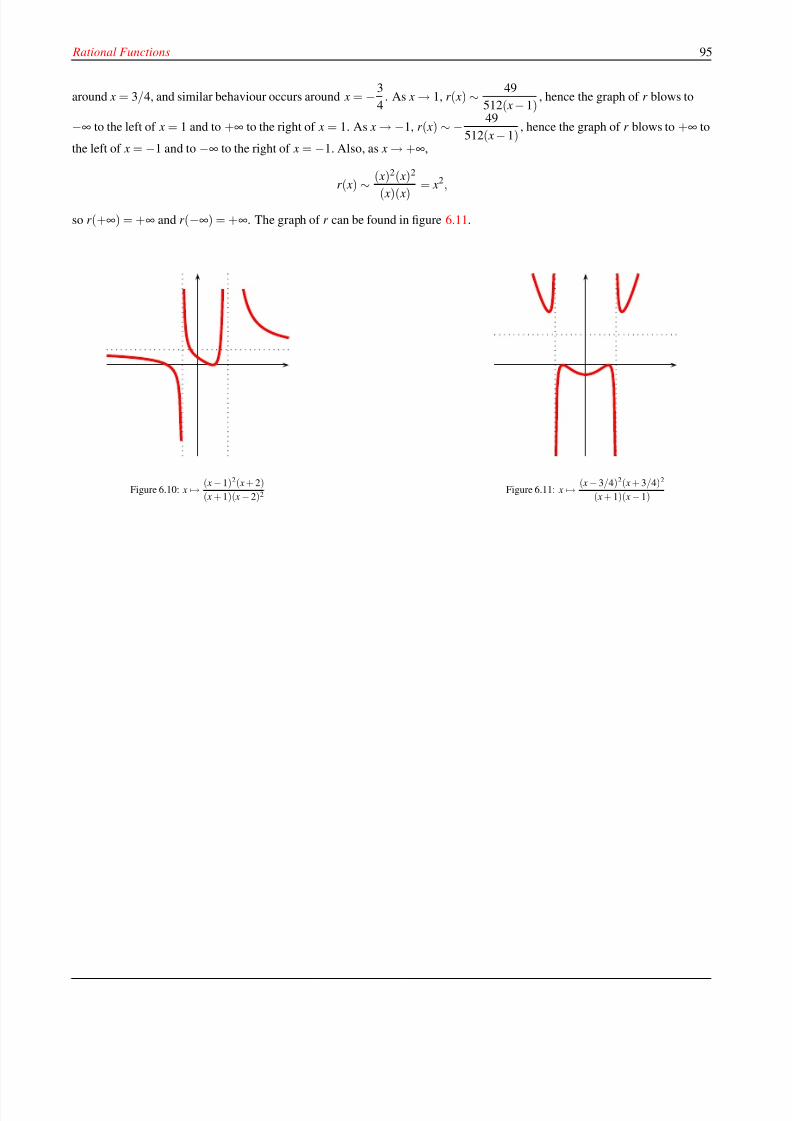
8/8/2019 Pre Calculus I
http://slidepdf.com/reader/full/pre-calculus-i 101/125
Rational Functions 95
around x = 3/4, and similar behaviour occurs around x = −3
4. As x → 1, r ( x) ∼ 49
512( x − 1), hence the graph of r blows to
−∞ to the left of x = 1 and to +∞ to the right of x = 1. As x → −1, r ( x) ∼ − 49
512( x − 1), hence the graph of r blows to +∞ to
the left of x = −1 and to −∞ to the right of x = −1. Also, as x → +∞,
r ( x)∼
( x)2( x)2
( x)( x)= x2,
so r (+∞) = +∞ and r (−∞) = +∞. The graph of r can be found in figure 6.11.
Figure 6.10: x → ( x −1)2( x + 2)
( x + 1)( x − 2)2Figure 6.11: x → ( x − 3/4)2( x + 3/4)2
( x + 1)( x −1)
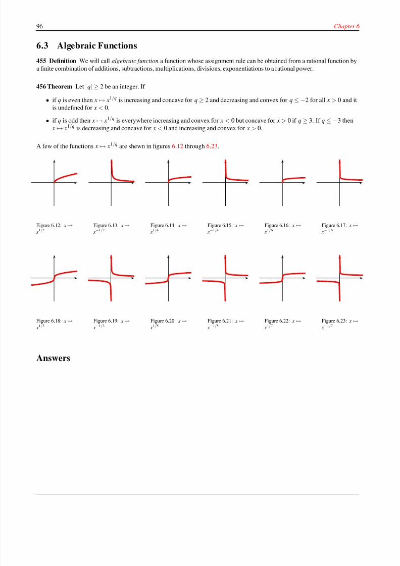
8/8/2019 Pre Calculus I
http://slidepdf.com/reader/full/pre-calculus-i 102/125
96 Chapter 6
6.3 Algebraic Functions
455 Definition We will call algebraic function a function whose assignment rule can be obtained from a rational function by
a finite combination of additions, subtractions, multiplications, divisions, exponentiations to a rational power.
456 Theorem Let |q| ≥ 2 be an integer. If
• if q is even then x → x1/q is increasing and concave for q ≥ 2 and decreasing and convex for q ≤ −2 for all x > 0 and itis undefined for x < 0.
• if q is odd then x → x1/q is everywhere increasing and convex for x < 0 but concave for x > 0 if q ≥ 3. If q ≤ −3 then
x → x1/q is decreasing and concave for x < 0 and increasing and convex for x > 0.
A few of the functions x → x1/q are shewn in figures 6.12 through 6.23.
Figure 6.12: x → x1/2
Figure 6.13: x → x−1/2
Figure 6.14: x → x1/4
Figure 6.15: x → x−1/4
Figure 6.16: x → x1/6
Figure 6.17: x → x−1/6
Figure 6.18: x → x1/3
Figure 6.19: x → x−1/3
Figure 6.20: x → x1/5
Figure 6.21: x → x−1/5
Figure 6.22: x → x1/7
Figure 6.23: x → x−1/7
Answers
8/8/2019 Pre Calculus I
http://slidepdf.com/reader/full/pre-calculus-i 103/125
Appendix
AComplex Numbers
A.1 Arithmetic of Complex Numbers
One uses the symbol i to denote the imaginary unit i =√
−1. Then i2 =
−1.
457 Example Find√−25.
Solution:√−25 = 5i.
Since i0 = 1, i1 = i, i2 = −1, i3 = −i, i4 = 1, i5 = i, etc., the powers of i repeat themselves cyclically in a cycle of period 4.
458 Example Find i1934.
Solution: Observe that 1934 = 4(483) + 2 and so i1934 = i2 = −1.
459 Example For any integral α one has
iα + iα +1 + iα +2 + iα +3 = iα (1 + i + i2 + i3) = iα (1 + i− 1 − i) = 0.
If a, b are real numbers then the object a + bi is called a complex number . One uses the symbol C to denote the set of all
complex numbers. If a, b, c, d ∈ R, then the sum of the complex numbers a + bi and c + di is naturally defined as
(a + bi) + (c + di) = (a + c) + (b + d )i (A.1)
The product of a + bi and c + di is obtained by multiplying the binomials:
(a + bi)(c + di) = ac + adi + bci + bdi2 = (ac − bd ) + (ad + bc)i (A.2)
460 Example Find the sum (4 + 3i) + (5 − 2i) and the product (4 + 3i)(5 − 2i).
Solution: One has
(4 + 3i) + (5 − 2i) = 9 + i
and
(4 + 3i)(5− 2i) = 20− 8i + 15i− 6i2 = 20 + 7i + 6 = 26 + 7i.
461 Definition Let z ∈ C, (a, b) ∈ R2 with z = a + bi. The conjugate z of z is defined by
z = a + bi = a − bi (A.3)
97
8/8/2019 Pre Calculus I
http://slidepdf.com/reader/full/pre-calculus-i 104/125
8/8/2019 Pre Calculus I
http://slidepdf.com/reader/full/pre-calculus-i 105/125
Equations involving Complex Numbers 99
Proof: By Theorem 463 , conjugation is multiplicative, hence
| z1 z2| =√
z1 z2 z1 z2
=√
z1 z2 z1 · z2
=√
z1 z1 z2 z2
= √ z1 z1√ z2 z2
= | z1|| z2|
whence the assertion follows. u
469 Example Write (22 + 32)(52 + 72) as the sum of two squares.
Solution: The idea is to write 22 + 32 = |2 + 3i|2, 52 + 72 = |5 + 7i|2 and use the multiplicativity of the modulus. Now
(22 + 32)(52 + 72) = |2 + 3i|2|5 + 7i|2
= |(2 + 3i)(5 + 7i)|2
= |− 11 + 29i|2
= 112 + 292
A.2 Equations involving Complex Numbers
Recall that if ux2 + vx + w = 0 with u = 0, then the roots of this equation are given by the Quadratic Formula
x = − v
2u±
√v2 − 4uw
2u(A.7)
The quantity v2 − 4uw under the square root is called the discriminant of the quadratic equation ux2 + vx + w = 0. If u, v, w are
real numbers and this discriminant is negative, one obtains complex roots.
Complex numbers thus occur naturally in the solution of quadratic equations. Since i2 = −1, one sees that x = i is a root of the
equation x2 + 1 = 0. Similary, x = −i is also a root of x2 + 1.
470 Example Solve 2 x2 + 6 x + 5 = 0
Solution: Using the quadratic formula
x = −6
4±
√−4
4= −3
2± i
1
2
In solving the problems that follow, the student might profit from the following identities.
s2 − t 2 = (s − t )(s + t ) (A.8)
s2k − t 2k = (sk − t k )(sk + t k ), k ∈ N (A.9)
s3 − t 3 = (s − t )(s2 + st + t 2) (A.10)
s3 + t 3 = (s + t )(s2 − st + t 2) (A.11)
471 Example Solve the equation x4 − 16 = 0.
Solution: One has x4 − 16 = ( x2 − 4)( x2 + 4) = ( x − 2)( x + 2)( x2 + 4). Thus either x = −2, x = 2 or x2 + 4 = 0. This last
equation has roots ±2i. The four roots of x4 − 16 = 0 are thus x = −2, x = 2, x = −2i, x = 2i.
8/8/2019 Pre Calculus I
http://slidepdf.com/reader/full/pre-calculus-i 106/125
100 Appendix A
472 Example Find the roots of x3 − 1 = 0.
Solution: x3 − 1 = ( x − 1)( x2 + x + 1). If x = 1, the two solutions to x2 + x + 1 = 0 can be obtained using the quadratic
formula, getting x = −1
2± i
√3
2.
473 Example Find the roots of x3
+ 8 = 0.
Solution: x3 + 8 = ( x + 2)( x2 − 2 x + 4). Thus either x = −2 or x2 − 2 x + 4 = 0. Using the quadratic formula, one sees that the
solutions of this last equation are x = 1 ± i√
3.
474 Example Solve the equation x4 + 9 x2 + 20 = 0.
Solution: One sees that
x4 + 9 x2 + 20 = ( x2 + 4)( x2 + 5) = 0
Thus either x2 + 4 = 0, in which case x = ±2i or x2 + 5 = 0 in which case x = ±i√
5. The four roots are x = ±2i,±i√
5
Homework
475 Problem Perform the following operations. Write your result
in the form a + bi, with (a, b) ∈ R2.
1.√
36 +√−36
2. (4 + 8i) − (9− 3i) + 5(2 + i)− 8i
3. 4 + 5i + 6i2 + 7i3
4. i(1 + i) + 2i2(3 −4i)
5. (8− 9i)(10 + 11i)
6. i1990 + i1991 + i1992 + i1993
7.2− i
2 + i
8. 1− i1 + 2i
+ 1 + i1 + 2i
9. (5 + 2i)2 + (5−2i)2
10. (1 + i)3
476 Problem Find real numbers a, b such that
(a−2) + (5b + 3)i = 4− 2i
477 Problem Write (22 + 32)(32 + 72) as the sum of two squares.
478 Problem Prove that (1 + i)2 = 2i and that (1− i)2 = −2i. Use
this to write
(1 + i)2004
(1 − i)2000
in the form a + bi, (a, b) ∈ R2.
479 Problem Prove that (1 + i√
3)3 = 8. Use this to prove that
(1 + i√
3)30 = 230.
480 Problem Find |5 + 7i|, |√
5 + 7i|, |5 + i√
7| and |√
5 + i√
7|.
481 Problem Prove that if k is an integer then
(4k +1)i4k +(4k +2)i4k +1 + (4k +3)i4k +2 +(4k +4)i4k +3 = −2−2i.
Use this to prove that
1 + 2i + 3i2 + 4i3 + · · ·+ 1995i1994 + 1996i1995 = −998 −998i.
482 Problem If z and z′ are complex numbers with either | z| = 1 or
| z′| = 1, prove that z − z′
1− zz′
= 1.
483 Problem Prove that if z, z′ and w are complex numbers with
| z
|=
| z′
|=
|w
|= 1, then
| zz′ + zw + z′w| = | z + z′ + w|
484 Problem Prove that if n is an integer which is not a multiple of
4 then
1n + in + i2n + i3n = 0.
Now let
f ( x) = (1 + x + x2)1000 = a0 + a1 x + · · ·+ a2000 x2000.
By considering f (1) + f (i) + f (i2) + f (i3), find
a0 + a4 + a8 + · · ·+ a2000.
485 Problem Find all the roots of the following equations.
1. x2 + 8 = 0
2. x2 + 49 = 0
3. x2 − 4 x + 5 = 0
4. x2 − 3 x + 6 = 0
5. x4 − 1 = 0
6. x4 + 2 x2 −3 = 0
7. x3 − 27 = 0
8. x6 − 1 = 0
9. x6 − 64 = 0

8/8/2019 Pre Calculus I
http://slidepdf.com/reader/full/pre-calculus-i 107/125
Appendix BSample Multiple-Choice Questions
101
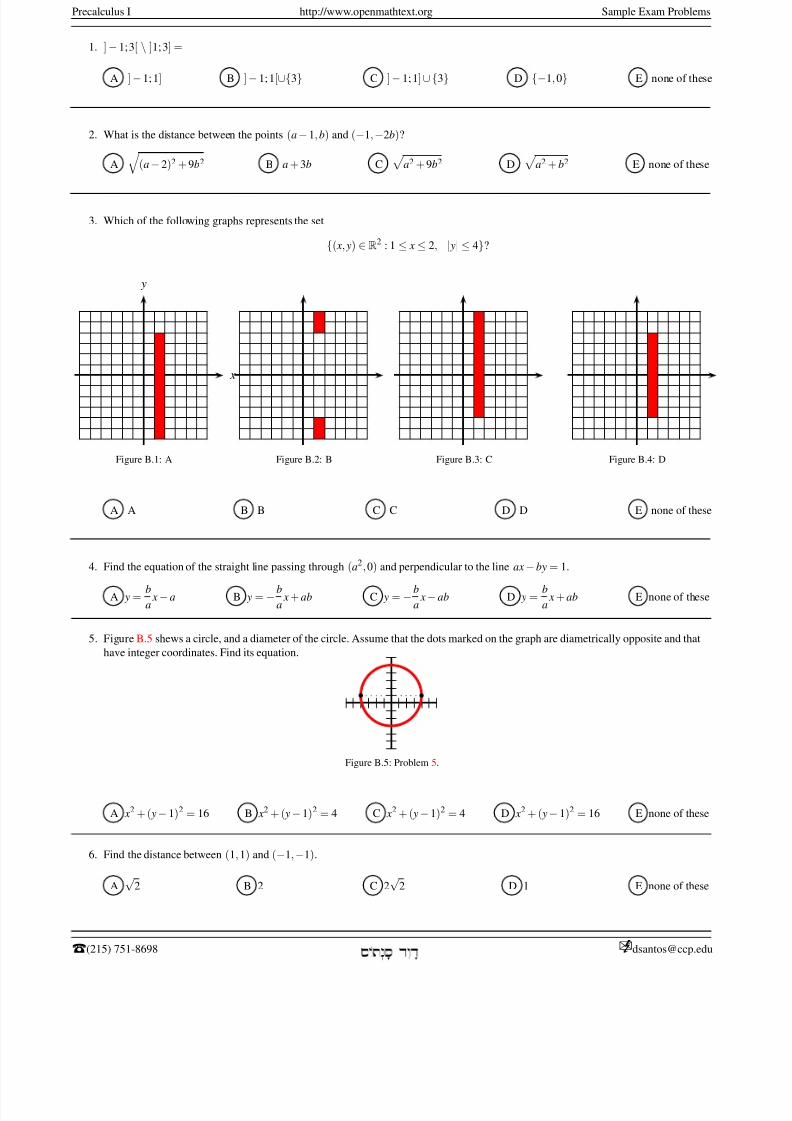
8/8/2019 Pre Calculus I
http://slidepdf.com/reader/full/pre-calculus-i 108/125
Precalculus I http://www.openmathtext.org Sample Exam Problems
1. ] − 1; 3[ \ ]1; 3] =
A ] −1; 1] B ]− 1; 1[∪{3} C ]− 1; 1]∪{3} D {−1, 0} E none of these
2. What is the distance between the points (a−1, b) and (−1,−2b)?
A
(a− 2)2 + 9b2 B a + 3b C
a2 + 9b2 D
a2 + b2 E none of these
3. Which of the following graphs represents the set
{( x, y) ∈R2 : 1 ≤ x ≤ 2, | y| ≤ 4}?
x
y
Figure B.1: A Figure B.2: B Figure B.3: C Figure B.4: D
A A B B C C D D E none of these
4. Find the equation of the straight line passing through (a2,0) and perpendicular to the line ax −by = 1.
A y =b
a x − a B y = −b
a x + ab C y = −b
a x− ab D y =
b
a x + ab E none of these
5. Figure B.5 shews a circle, and a diameter of the circle. Assume that the dots marked on the graph are diametrically opposite and that
have integer coordinates. Find its equation.
Figure B.5: Problem 5.
A x2 + ( y− 1)2 = 16 B x2 + ( y −1)2 = 4 C x2 + ( y −1)2 = 4 D x2 + ( y− 1)2 = 16 E none of these
6. Find the distance between (1, 1) and (−1,−1).
A√
2 B 2 C 2√
2 D 1 E none of these
T(215) 751-8698 [email protected]á ê à á
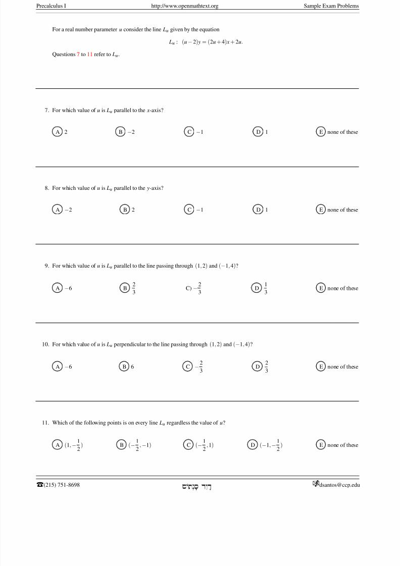
8/8/2019 Pre Calculus I
http://slidepdf.com/reader/full/pre-calculus-i 109/125
Precalculus I http://www.openmathtext.org Sample Exam Problems
For a real number parameter u consider the line Lu given by the equation
Lu : (u −2) y = (2u + 4) x + 2u.
Questions 7 to 11 refer to Lu.
7. For which value of u is Lu parallel to the x-axis?
A 2 B −2 C −1 D 1 E none of these
8. For which value of u is Lu parallel to the y-axis?
A −2 B 2 C −1 D 1 E none of these
9. For which value of u is Lu parallel to the line passing through (1, 2) and (−1, 4)?
A
−6 B
2
3
C)
−2
3
D1
3
E none of these
10. For which value of u is Lu perpendicular to the line passing through (1, 2) and (−1, 4)?
A −6 B 6 C −2
3D
2
3E none of these
11. Which of the following points is on every line Lu regardless the value of u?
A (1,−1
2) B (−1
2,−1) C (−1
2,1) D (−1,−1
2) E none of these
T(215) 751-8698 [email protected]á ê à á
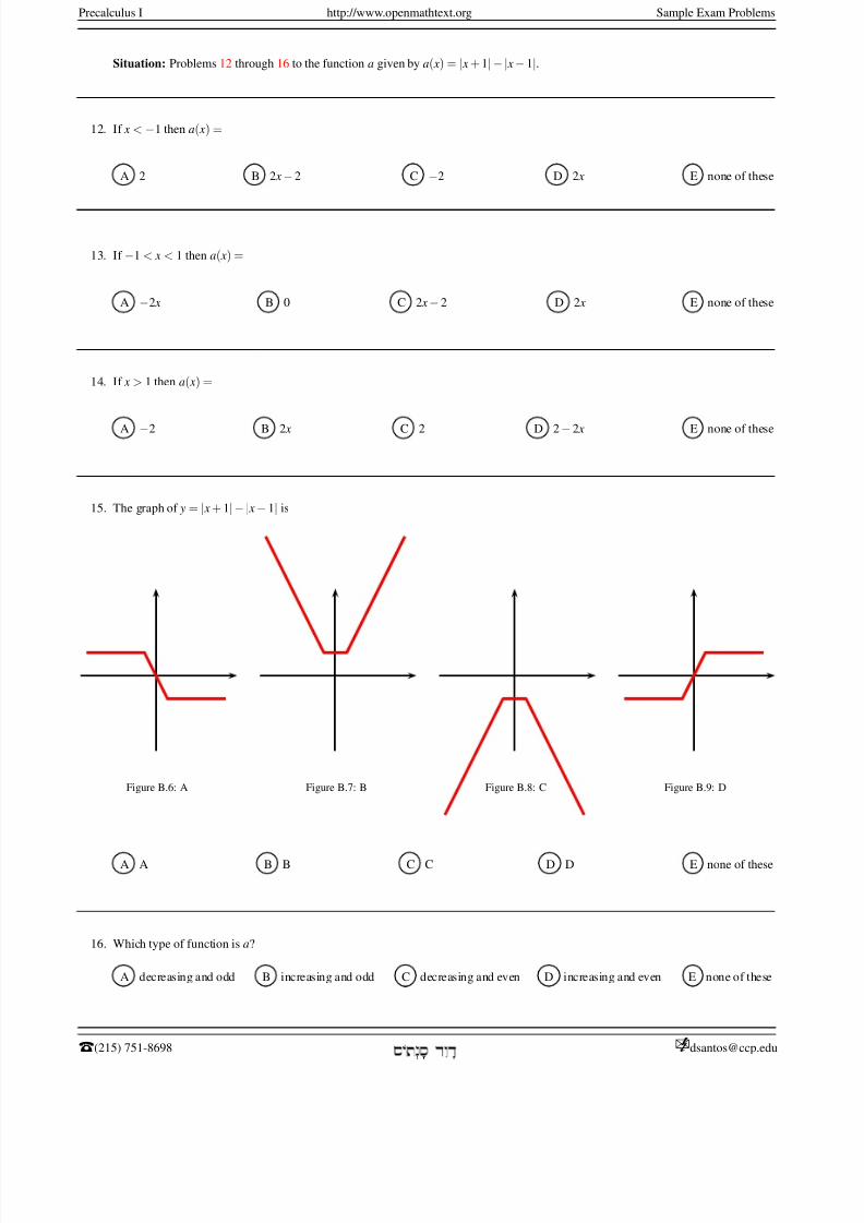
8/8/2019 Pre Calculus I
http://slidepdf.com/reader/full/pre-calculus-i 110/125
Precalculus I http://www.openmathtext.org Sample Exam Problems
Situation: Problems 12 through 16 to the function a given by a( x) = | x + 1|− | x− 1|.
12. If x < −1 then a( x) =
A 2 B 2 x −2 C −2 D 2 x E none of these
13. If −1 < x < 1 then a( x) =
A −2 x B 0 C 2 x− 2 D 2 x E none of these
14. If x > 1 then a( x) =
A −2 B 2 x C 2 D 2− 2 x E none of these
15. The graph of y = | x + 1|− | x − 1| is
Figure B.6: A Figure B.7: B Figure B.8: C Figure B.9: D
A A B B C C D D E none of these
16. Which type of function is a?
A decreasing and odd B increasing and odd C decreasing and even D increasing and even E none of these
T(215) 751-8698 [email protected]á ê à á
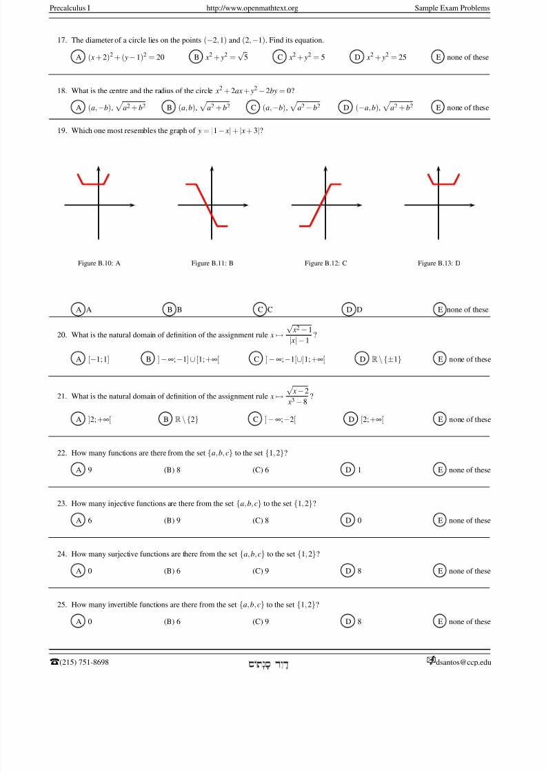
8/8/2019 Pre Calculus I
http://slidepdf.com/reader/full/pre-calculus-i 111/125
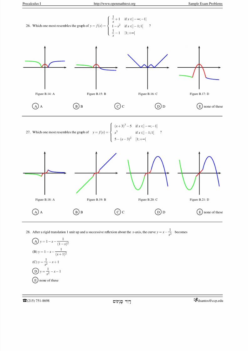
8/8/2019 Pre Calculus I
http://slidepdf.com/reader/full/pre-calculus-i 112/125
Precalculus I http://www.openmathtext.org Sample Exam Problems
26. Which one most resembles the graph of y = f ( x) =
1
x+ 1 if x ∈]−∞;−1]
1 − x2 if x ∈]− 1; 1[1
x− 1 [1; +∞[
?
Figure B.14: A Figure B.15: B Figure B.16: C Figure B.17: D
A A B B C C D D E none of these
27. Which one most resembles the graph of y = f ( x) =
( x + 3)2 − 5 if x ∈] −∞;−1]
x3 if x ∈] −1; 1[
5− ( x − 3)2 [1; +∞[
?
Figure B.18: A Figure B.19: B Figure B.20: C Figure B.21: D
A A B B C C D D E none of these
28. After a rigid translation 1 unit up and a successive reflexion about the x-axis, the curve y = x− 1
x2becomes
A y = 1− x −1
(1− x)2
(B) y = 1− x − 1
( x + 1)2
(C) y =1
x2− x + 1
D y =1
x2− x− 1
E none of these
T(215) 751-8698 [email protected]á ê à á
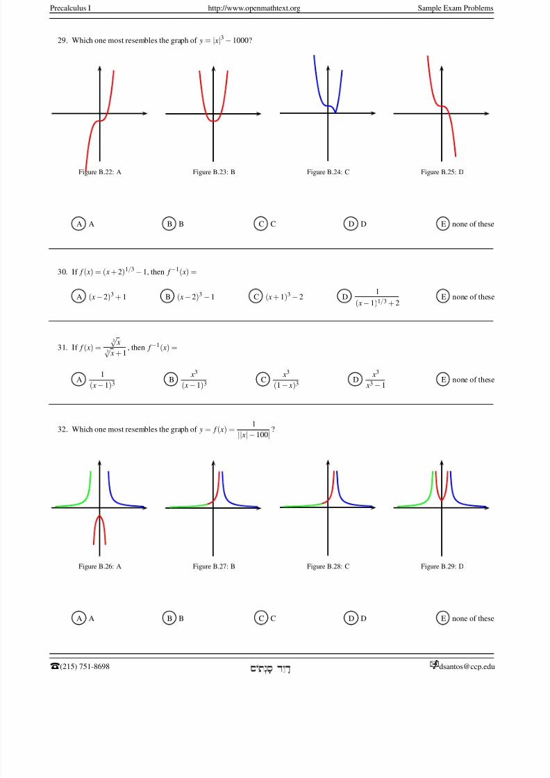
8/8/2019 Pre Calculus I
http://slidepdf.com/reader/full/pre-calculus-i 113/125
Precalculus I http://www.openmathtext.org Sample Exam Problems
29. Which one most resembles the graph of y = | x|3 − 1000?
Figure B.22: A Figure B.23: B Figure B.24: C Figure B.25: D
A A B B C C D D E none of these
30. If f ( x) = ( x + 2)1/3 −1, then f −1( x) =
A ( x −2)3 + 1 B ( x −2)3 −1 C ( x + 1)3 −2 D1
( x− 1)1/3 + 2E none of these
31. If f ( x) =3√
x3√
x + 1, then f −1( x) =
A1
( x− 1)3B
x3
( x −1)3C
x3
(1 − x)3D
x3
x3 − 1E none of these
32. Which one most resembles the graph of y = f ( x) =1
|| x|−100|?
Figure B.26: A Figure B.27: B Figure B.28: C Figure B.29: D
A A B B C C D D E none of these
T(215) 751-8698 [email protected]á ê à á
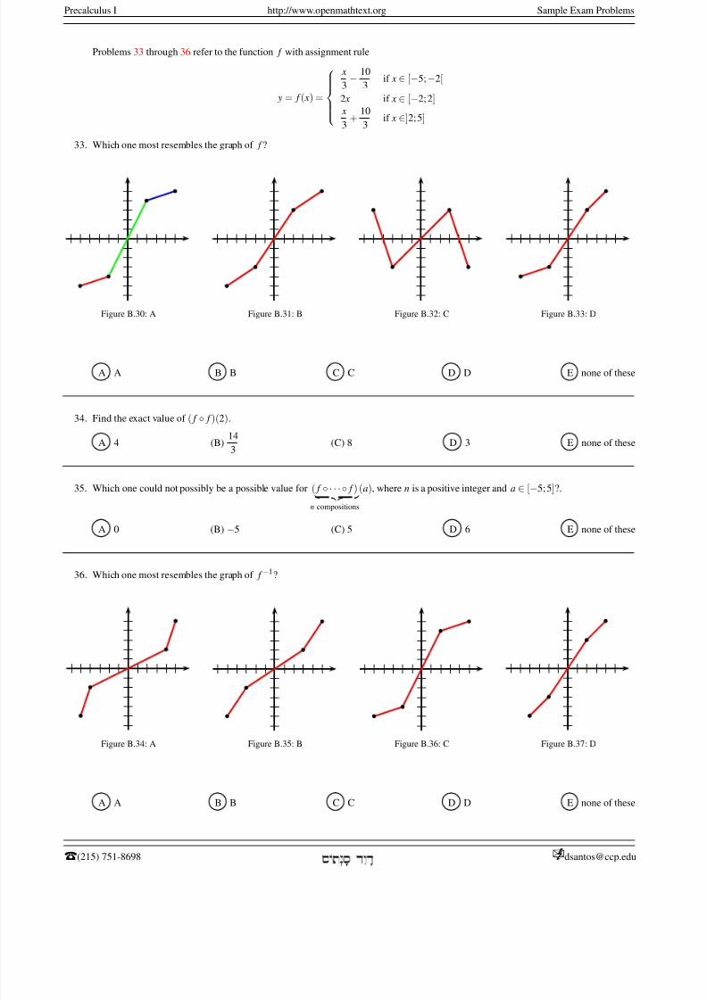
8/8/2019 Pre Calculus I
http://slidepdf.com/reader/full/pre-calculus-i 114/125
Precalculus I http://www.openmathtext.org Sample Exam Problems
Problems 33 through 36 refer to the function f with assignment rule
y = f ( x) =
x
3− 10
3if x ∈ [−5;−2[
2 x if x ∈ [−2; 2] x
3+
10
3if x ∈]2; 5]
33. Which one most resembles the graph of f ?
Figure B.30: A
Figure B.31: B
Figure B.32: C
Figure B.33: D
A A B B C C D D E none of these
34. Find the exact value of ( f ◦ f )(2).
A 4 (B)14
3(C) 8 D 3 E none of these
35. Which one could not possibly be a possible value for ( f ◦ · · · ◦ f )
n compositions
(a), where n is a positive integer and a ∈ [−5; 5]?.
A 0 (B) −5 (C) 5 D 6 E none of these
36. Which one most resembles the graph of f −1?
Figure B.34: A
Figure B.35: B
Figure B.36: C
Figure B.37: D
A A B B C C D D E none of these
T(215) 751-8698 [email protected]á ê à á
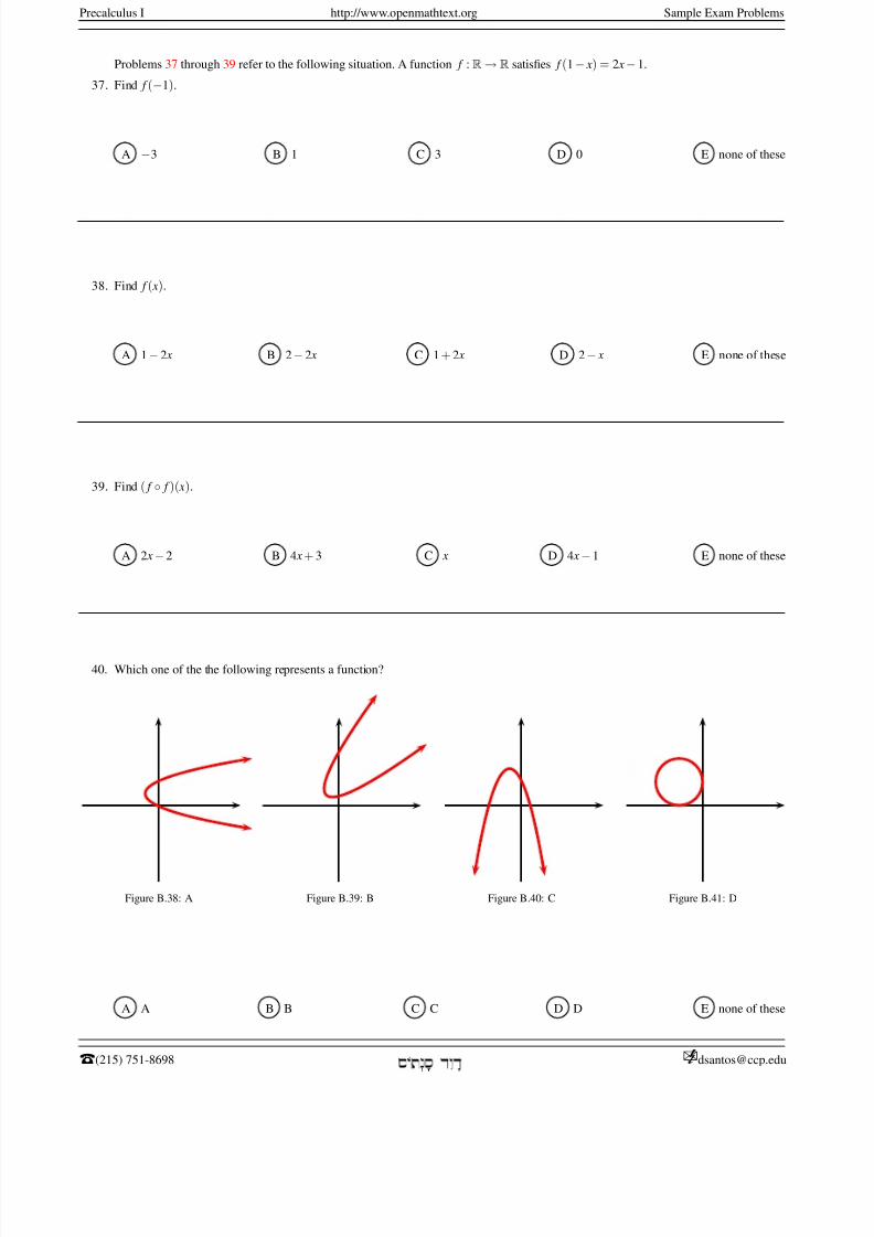
8/8/2019 Pre Calculus I
http://slidepdf.com/reader/full/pre-calculus-i 115/125
Precalculus I http://www.openmathtext.org Sample Exam Problems
Problems 37 through 39 refer to the following situation. A function f :R→R satisfies f (1− x) = 2 x− 1.
37. Find f (−1).
A −3 B 1 C 3 D 0 E none of these
38. Find f ( x).
A 1− 2 x B 2− 2 x C 1 + 2 x D 2− x E none of these
39. Find ( f ◦ f )( x).
A 2 x −2 B 4 x + 3 C x D 4 x −1 E none of these
40. Which one of the the following represents a function?
Figure B.38: A Figure B.39: B Figure B.40: C Figure B.41: D
A A B B C C D D E none of these
T(215) 751-8698 [email protected]á ê à á
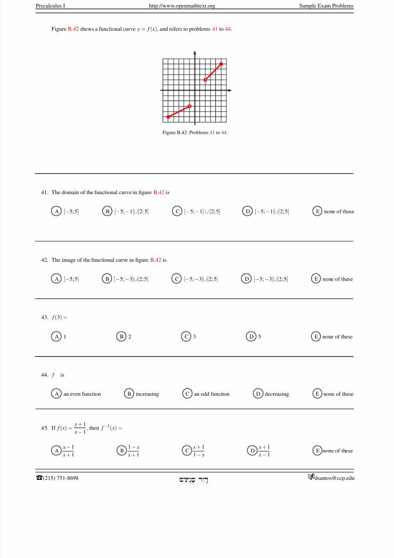
8/8/2019 Pre Calculus I
http://slidepdf.com/reader/full/pre-calculus-i 116/125
Precalculus I http://www.openmathtext.org Sample Exam Problems
Figure B.42 shews a functional curve y = f ( x), and refers to problems 41 to 44.
Figure B.42: Problems 41 to 44.
41. The domain of the functional curve in figure B.42 is
A [−5; 5] B [−5;−1[∪]2; 5] C [−5;−1]∪ [2; 5] D [−5;−1[∪[2; 5[ E none of these
42. The image of the functional curve in figure B.42 is
A [−5; 5] B [−5;−3]∪]2; 5] C [−5;−3[∪]2; 5[ D [−5;−3[∪]2; 5[ E none of these
43. f (3) =
A 1 B 2 C 3 D 5 E none of these
44. f is
A an even function B increasing C an odd function D decreasing E none of these
45. If f ( x) =x + 1
x −1, then f −1( x) =
Ax− 1
x + 1B
1− x
x + 1C
x + 1
1− xD
x + 1
x− 1E none of these
T(215) 751-8698 [email protected]á ê à á
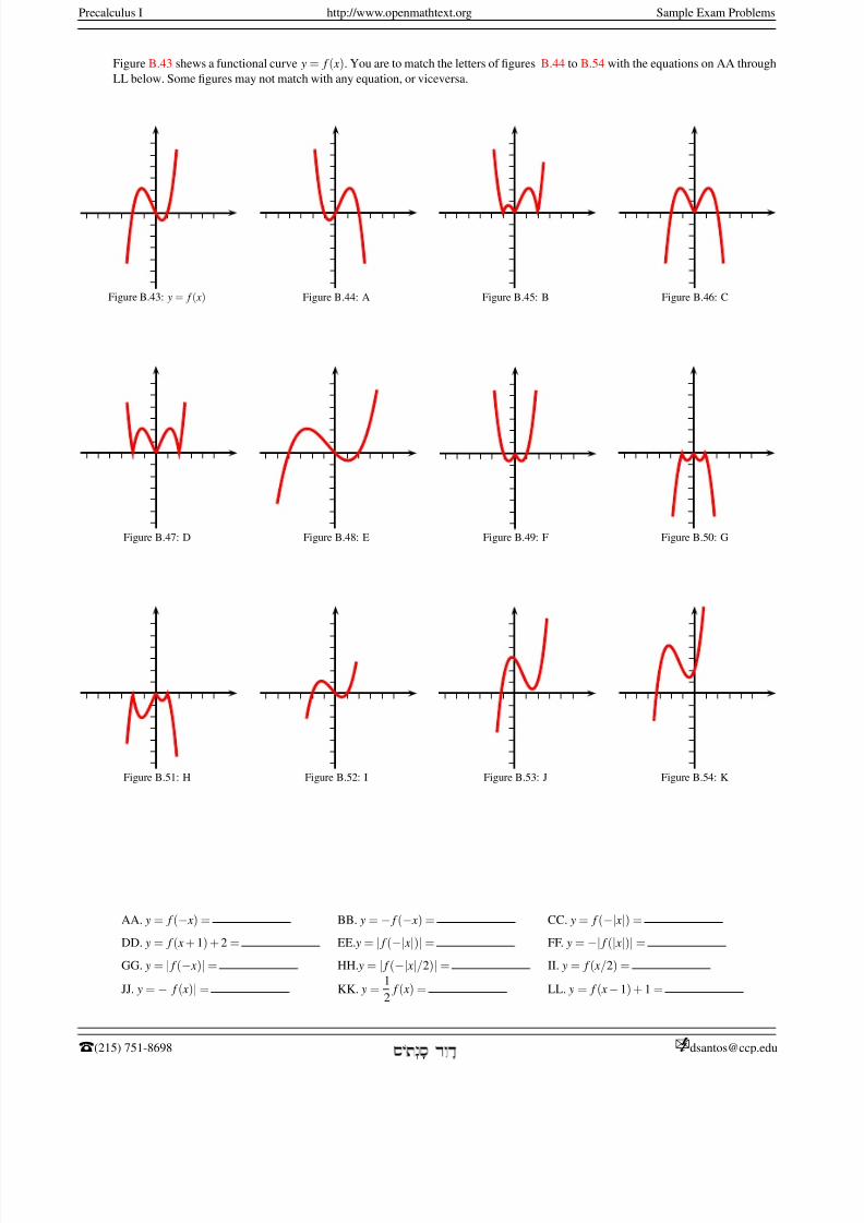
8/8/2019 Pre Calculus I
http://slidepdf.com/reader/full/pre-calculus-i 117/125
Precalculus I http://www.openmathtext.org Sample Exam Problems
Figure B.43 shews a functional curve y = f ( x). You are to match the letters of figures B.44 to B.54 with the equations on AA through
LL below. Some figures may not match with any equation, or viceversa.
Figure B.43: y = f ( x) Figure B.44: A Figure B.45: B Figure B.46: C
Figure B.47: D Figure B.48: E Figure B.49: F Figure B.50: G
Figure B.51: H Figure B.52: I Figure B.53: J Figure B.54: K
AA. y = f (− x) = BB. y = − f (− x) = CC. y = f (−| x|) =
DD. y = f ( x + 1) + 2 = EE. y = | f (−| x|)| = FF. y = −| f (| x|)| =
GG. y = | f (− x)| = HH. y = | f (−| x|/2)| = II. y = f ( x/2) =
JJ. y = −| f ( x)| = KK. y =1
2f ( x) = LL. y = f ( x −1) + 1 =
T(215) 751-8698 [email protected]á ê à á
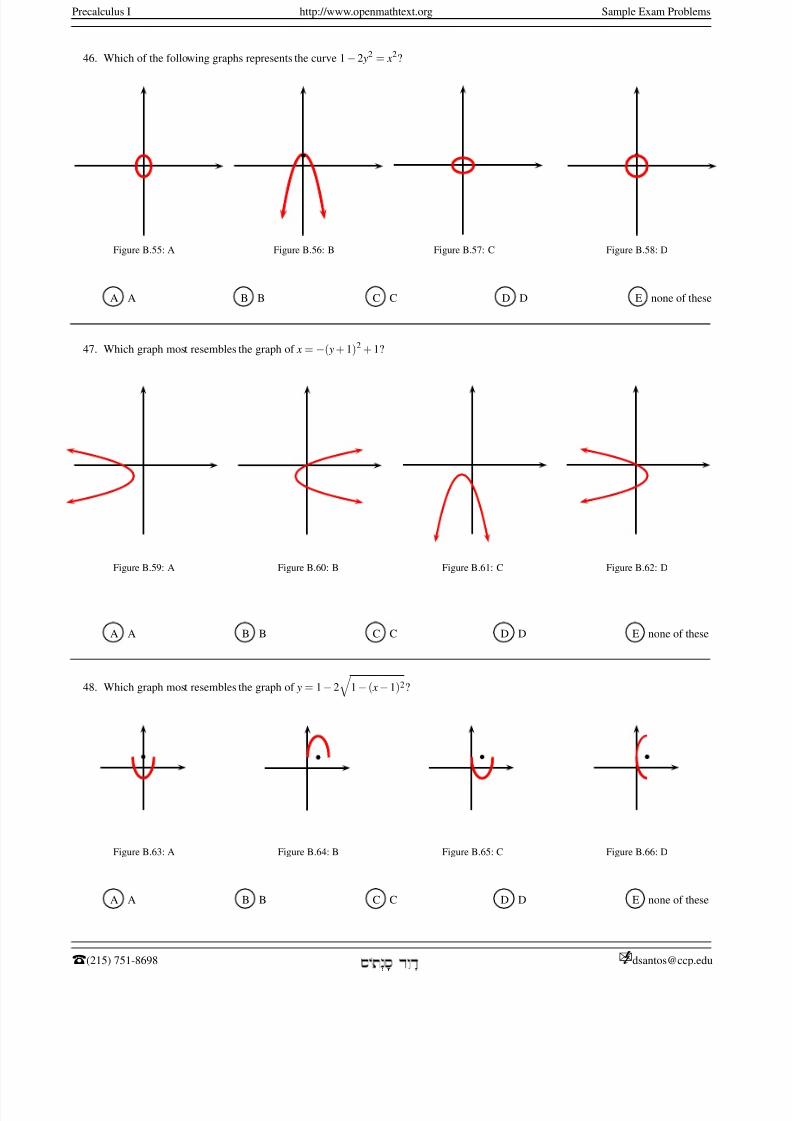
8/8/2019 Pre Calculus I
http://slidepdf.com/reader/full/pre-calculus-i 118/125
Precalculus I http://www.openmathtext.org Sample Exam Problems
46. Which of the following graphs represents the curve 1−2 y2 = x2?
Figure B.55: A
Figure B.56: B Figure B.57: C
Figure B.58: D
A A B B C C D D E none of these
47. Which graph most resembles the graph of x = −( y + 1)2 + 1?
Figure B.59: A Figure B.60: B Figure B.61: C Figure B.62: D
A A B B C C D D E none of these
48. Which graph most resembles the graph of y = 1−2
1− ( x −1)2?
Figure B.63: A
Figure B.64: B
Figure B.65: C
Figure B.66: D
A A B B C C D D E none of these
T(215) 751-8698 [email protected]á ê à á
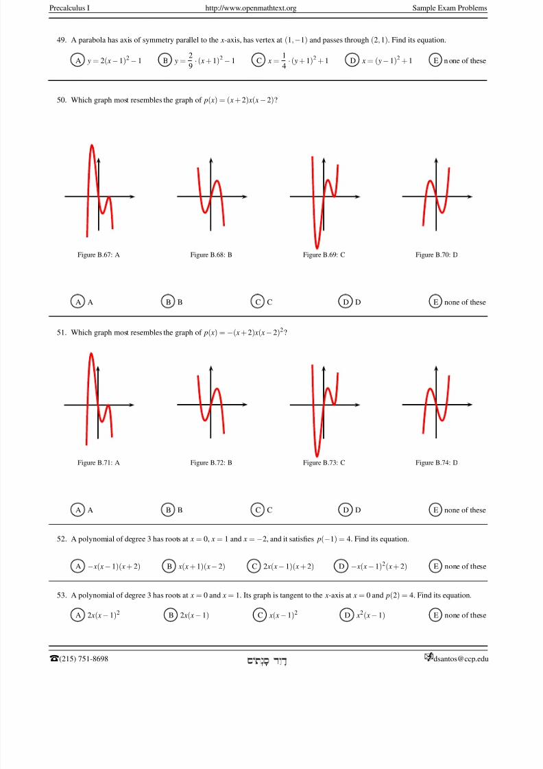
8/8/2019 Pre Calculus I
http://slidepdf.com/reader/full/pre-calculus-i 119/125
Precalculus I http://www.openmathtext.org Sample Exam Problems
49. A parabola has axis of symmetry parallel to the x-axis, has vertex at (1,−1) and passes through (2, 1). Find its equation.
A y = 2( x −1)2 − 1 B y =2
9· ( x + 1)2 − 1 C x =
1
4· ( y + 1)2 + 1 D x = ( y− 1)2 + 1 E n one of these
50. Which graph most resembles the graph of p( x) = ( x + 2) x( x −2)?
Figure B.67: A Figure B.68: B Figure B.69: C Figure B.70: D
A A B B C C D D E none of these
51. Which graph most resembles the graph of p( x) = −( x + 2) x( x − 2)2?
Figure B.71: A Figure B.72: B Figure B.73: C Figure B.74: D
A A B B C C D D E none of these
52. A polynomial of degree 3 has roots at x = 0, x = 1 and x = −2, and it satisfies p(−1) = 4. Find its equation.
A − x( x− 1)( x + 2) B x( x + 1)( x− 2) C 2 x( x− 1)( x + 2) D − x( x −1)2( x + 2) E none of these
53. A polynomial of degree 3 has roots at x = 0 and x = 1. Its graph is tangent to the x-axis at x = 0 and p(2) = 4. Find its equation.
A 2 x( x − 1)2 B 2 x( x −1) C x( x −1)2 D x2( x− 1) E none of these
T(215) 751-8698 [email protected]á ê à á
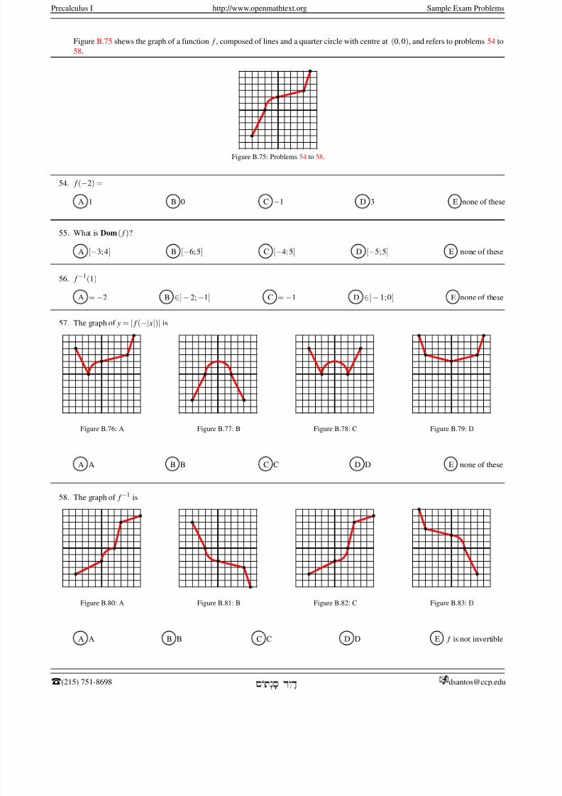
8/8/2019 Pre Calculus I
http://slidepdf.com/reader/full/pre-calculus-i 120/125
Precalculus I http://www.openmathtext.org Sample Exam Problems
Figure B.75 shews the graph of a function f , composed of lines and a quarter circle with centre at (0, 0), and refers to problems 54 to
58.
Figure B.75: Problems 54 to 58.
54. f (−2) =
A 1 B 0 C −1 D 3 E none of these
55. What is Dom ( f )?
A [−3; 4] B [−6; 5] C [−4; 5] D [−5; 5] E none of these
56. f −1(1)
A = −2 B ∈]− 2;−1[ C = −1 D ∈]− 1; 0[ E none of these
57. The graph of y = | f (−| x|)| is
Figure B.76: A
Figure B.77: B
Figure B.78: C
Figure B.79: D
A A B B C C D D E none of these
58. The graph of f −1 is
Figure B.80: A
Figure B.81: B
Figure B.82: C
Figure B.83: D
A A B B C C D D E f is not invertible
T(215) 751-8698 [email protected]á ê à á
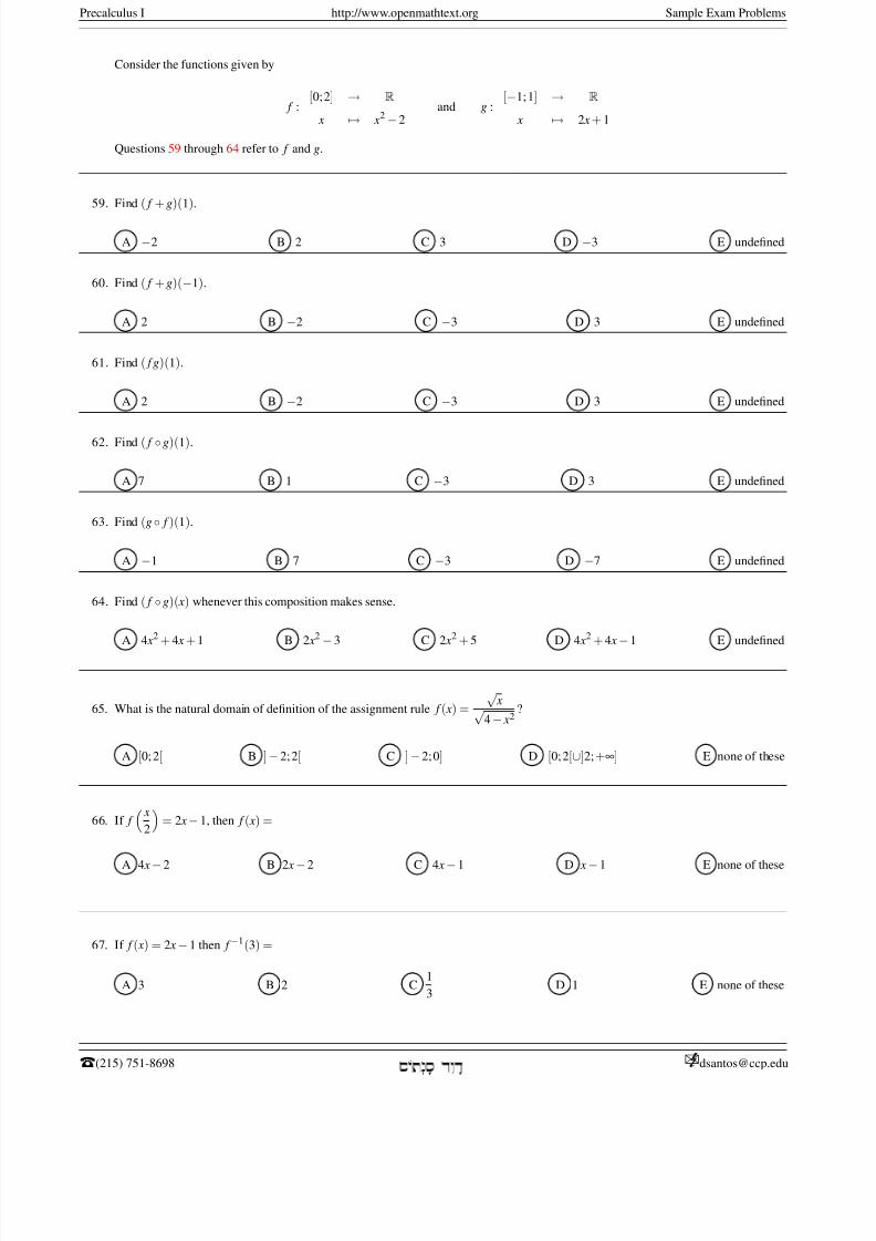
8/8/2019 Pre Calculus I
http://slidepdf.com/reader/full/pre-calculus-i 121/125
Precalculus I http://www.openmathtext.org Sample Exam Problems
Consider the functions given by
f :[0; 2] → R
x → x2 −2and g :
[−1; 1] → R
x → 2 x + 1
Questions 59 through 64 refer to f and g.
59. Find ( f + g)(1).
A −2 B 2 C 3 D −3 E undefined
60. Find ( f + g)(−1).
A 2 B −2 C −3 D 3 E undefined
61. Find ( f g)(1).
A 2 B −2 C −3 D 3 E undefined
62. Find ( f ◦ g)(1).
A 7 B 1 C −3 D 3 E undefined
63. Find (g◦ f )(1).
A −1 B 7 C −3 D −7 E undefined
64. Find ( f ◦ g)( x) whenever this composition makes sense.
A 4 x2
+ 4 x + 1 B 2 x2
− 3 C 2 x2
+ 5 D 4 x2
+ 4 x −1 E undefined
65. What is the natural domain of definition of the assignment rule f ( x) =
√ x√
4 − x2?
A [0; 2[ B ]− 2; 2[ C ] −2; 0] D [0; 2[∪]2; +∞] E none of these
66. If f x
2
= 2 x− 1, then f ( x) =
A 4 x− 2 B 2 x −2 C 4 x −1 D x −1 E none of these
67. If f ( x) = 2 x − 1 then f −1(3) =
A 3 B 2 C1
3D 1 E none of these
T(215) 751-8698 [email protected]á ê à á
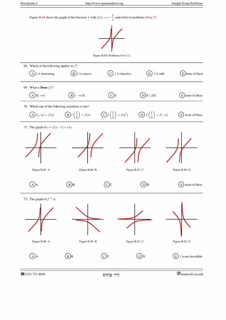
8/8/2019 Pre Calculus I
http://slidepdf.com/reader/full/pre-calculus-i 122/125
Precalculus I http://www.openmathtext.org Sample Exam Problems
Figure B.84 shews the graph of the function f with f ( x) = x− 1
x, and refers to problems 68 to 72.
Figure B.84: Problems 68 to 72.
68. Which of the following applies to f ?
A f is increasing B f is convex C f is injective D f is odd E none of these
69. What is Dom ( f )?
A ]0; +∞[ B ] −∞; 0[ C R D R\{0} E none of these
70. Which one of the following assertions is true?
A f (−a) = f (a) B f
1
a
= f (a) C f
1
a
= f (a2) D f
1
a
= f (−a) E none of these
71. The graph of y = f ( x −1) + 1 is
Figure B.85: A Figure B.86: B Figure B.87: C Figure B.88: D
A A B B C C D D E none of these
72. The graph of f −1 is
Figure B.89: A Figure B.90: B Figure B.91: C Figure B.92: D
A A B B C C D D E f is not invertible
T(215) 751-8698 [email protected]á ê à á
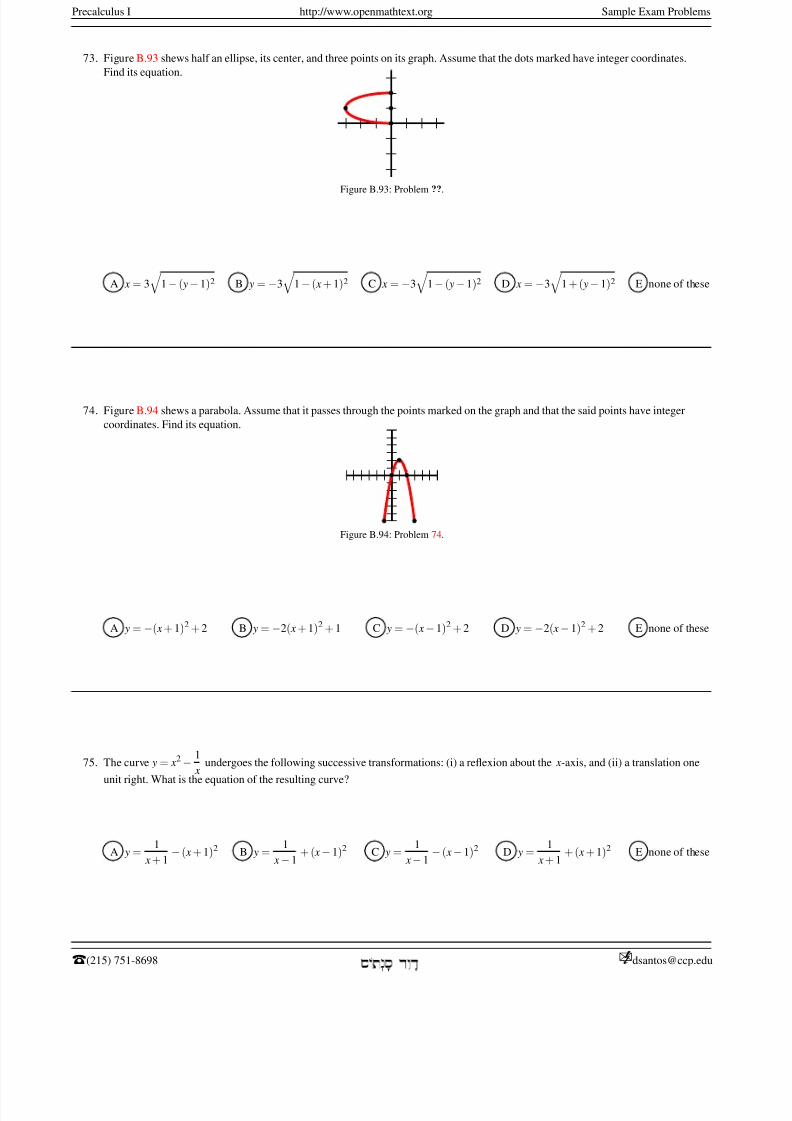
8/8/2019 Pre Calculus I
http://slidepdf.com/reader/full/pre-calculus-i 123/125
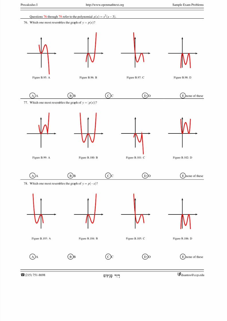
8/8/2019 Pre Calculus I
http://slidepdf.com/reader/full/pre-calculus-i 124/125
Precalculus I http://www.openmathtext.org Sample Exam Problems
Questions 76 through 78 refer to the polynomial p( x) = x2( x− 3).
76. Which one most resembles the graph of y = p( x)?
Figure B.95: A Figure B.96: B Figure B.97: C Figure B.98: D
A A B B C C D D E none of these
77. Which one most resembles the graph of y = | p( x)|?
Figure B.99: A Figure B.100: B Figure B.101: C Figure B.102: D
A A B B C C D D E none of these
78. Which one most resembles the graph of y = p(− x)?
Figure B.103: A Figure B.104: B Figure B.105: C Figure B.106: D
A A B B C C D D E none of these
T(215) 751-8698 [email protected]á ê à á

8/8/2019 Pre Calculus I
http://slidepdf.com/reader/full/pre-calculus-i 125/125
Bibliography
[Apo] Apostol, T. M., Calculus, Vol 1 & 2, 2nd ed., Waltham: Xerox, 1967.
[Art] Artino, R., Gaglione, A., and Shell, N., The Contest Problem Book IV, Mathematical Association of America.
[Har] Hardy, G. H., Pure Mathematics, 10th ed., New York: Cambridge University Press, 1952.
[Kla] Klambauer, Gabriel, Aspects of Calculus, New York: Springer-Verlag, 1986.
[Gel1] Gelfand, I.M., Glagoleva, E.G., Kirillov, A.A. The Method of Coordinates, Mineola, New York: Dover Publications, Inc., 2002.
[Gel2] Gelfand, I.M., Glagoleva, E.G., Shnol, E.E. Functions and Graphs , Mineola, New York: Dover Publications, Inc., 2002.
[Lan] Landau, E., Differential and Integral Calculus, New York, Chelsea Publishing Company, 1950.
[Olm] Olmstead, J. M. H., Calculus with Analytic Geometry, Vol 1 & 2, New York: Appleton-Century-Crofts, 1966.
[Par] Parsonson, S. L., Pure Mathematics, Vol 1 & 2, New York: Cambridge University Press, 1970.
[Spi] Spivak, Michael Calculus, 3rd ed., Houston, Texas: Publish or Perish, Inc., 1994.