pratik meshram-Unit 5 (contemporary mkt r sch)

Unit 5

Data Analysis-II

TOPICS5.1 Cluster Analysis5.2 Multidimensional Scaling5.3 Perceptual Mapping5.4 Discriminant Analysis

Analysis of data is the process of evaluating data using analytical and logical reasoning to examine each component of the data provided. This form of analysis is just one of the many steps that must be completed when conducting a research experiment. Data from various sources is gathered, reviewed, and then analyzed to form some sort of finding or conclusion. There are a variety of specific data analysis method, some of which include data mining, text analytics, business intelligence, and data visualizations. It is a process of inspecting, cleaning, transforming, and modeling data with the goal of discovering useful information, suggesting conclusions, and supporting decision making.Data analysis has multiple facets and approaches, encompassing diverse techniques under a variety of names, in different business, science, and social science domains.

Introduction

5.1 Cluster Analysis

Grouping similar customers and products is a fundamental marketing activity. It issued, prominently, in market segmentation. As companies cannot connect with all their customers, they have to divide markets into groups of consumers, customers, or clients (called segments) with similar needs and wants. Firms can then target each of these segments by positioning themselves in a unique segment (such as Ferrari in the high-end sports car market).

A) Meaning:Cluster analysis embraces a variety of techniques, the main objective of which is to group observations or variables into homogeneous and distinct clusters. A simple numerical example will help explain these objectives


B) Example:The daily expenditures on food (X1) and clothing (X2) of persons are shown in following Table.

The numbers are fictitious and not at all realistic, but the example will help us explain the essential features of cluster analysis as simply as possible. The data of Table are plotted in next figure.

Person X1 X2

A 2 4

B 8 2

C 9 3

D 1 5

e 8.5 1

.a

.c

.d

.e.b

X2

5

10

o


B) Example:

Inspection of figure suggests that the observations from two clusters. The consists of persons ‘A’ and ‘D’, and the second of b, c and e. It can be noted that the observations in each cluster are similar to one another with respect to expenditures on food and clothing, and that the two clusters are quite distinct from each other.These conclusions concerning the number of clusters and their membership were reached through a visual inspection of figure. This inspection was possible bemuse only two variables were involved in grouping the observations.


C) Examples of Clustering Applications:Marketing

Land use

Insurance

City-planning

Earth-quake studies


C) Examples of Clustering Applications:1) Marketing:

Help marketers discover distinct groups in their customer bases, and then use this knowledge to develop targeted marketing programs.

2) Land use:Identification of areas of similar land use in an earth observation database.

3) Insurance:Identifying groups of motor insurance policy holders with a high average claim cost.

4) City-planning:Identifying groups of houses according to their house type, value, and geographical location.

5) Earth-quake studies:Observed earth quake epicenters should be clustered along continent faults.


D) Types of Data required to Clustering in Data Mining:Scalability

Versatility

Discover Clusters

Minimal Input

Parameter

High Dimensio

nality

Ability to Deal with

Noisy Data

Interpretability


D) Types of Data required to Clustering in Data Mining:1) Scalability:

The cluster method should be applicable to huge databases and should decrease linearly with data size increase.

2) Versatility:Clustering objects could be of different types – numerical data, Boolean data or categorical data. Ideally a clustering method should be suitable for all different types of data objects.

3) Ability to Discover Clusters with Different Shapes:This is an important requirement for spatial data clustering. Many clustering algorithms can only discover clusters with spherical shapes.

4) Minimal Input Parameter:The method should require a minimum amount of domain knowledge for correct clustering. However, most current clustering algorithms have several key parameters and they are thus not practical for use in real world applications.


D) Types of Data required to Clustering in Data Mining:

5) High Dimensionality:The clustering algorithm should not only be able to handle low- dimensional data but also the high dimensional space.

6) Ability to Deal with Noisy Data:Databases contain noisy, missing or erroneous data. Some algorithms are sensitive to such data and may lead to poor quality clusters.

7) Interpretability:The clustering results should be interpretable, comprehensible and usable.


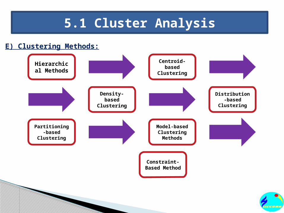
E) Clustering Methods:

Hierarchical Methods

Centroid-based

Clustering

Distribution-based

Clustering

Density-based

Clustering

Partitioning-based

Clustering

Model-based Clustering Methods

Constraint-Based

Method



1) Hierarchical Methods:Hierarchical clustering procedures are characterized by the tree-like structure established in the course of the analysis. Most hierarchical techniques fall into category called agglomerative clustering. In this category, clusters are consecutively formed from objects. Initially, this type of procedure starts with each object representing an individual cluster.

2) Centroid-based Clustering:In centroid-based clustering, clusters are represented by a central vector, which may not necessarily be a member of the data set. When the number of clusters is fixed to k, k-means clustering gives a formal definition as an optimization problem: find the cluster centers and assign the objects to the nearest cluster center, such that the squared distances from the cluster are minimized.



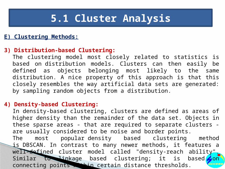
3) Distribution-based Clustering:The clustering model most closely related to statistics is based on distribution models. Clusters can then easily be defined as objects belonging most likely to the same distribution. A nice property of this approach is that this closely resembles the way artificial data sets are generated: by sampling random objects from a distribution.

4) Density-based Clustering:In density-based clustering, clusters are defined as areas of higher density than the remainder of the data set. Objects in these sparse areas - that are required to separate clusters - are usually considered to be noise and border points.The most popular density based clustering method is DBSCAN. In contrast to many newer methods, it features a well-defined cluster model called "density-reach ability". Similar to linkage based clustering; it is based on connecting points within certain distance thresholds.


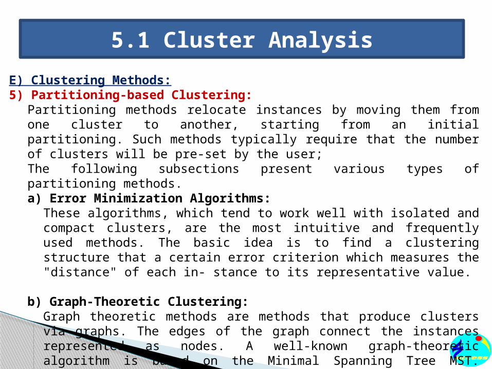
E) Clustering Methods:5) Partitioning-based Clustering:

Partitioning methods relocate instances by moving them from one cluster to another, starting from an initial partitioning. Such methods typically require that the number of clusters will be pre-set by the user;The following subsections present various types of partitioning methods.a) Error Minimization Algorithms:

These algorithms, which tend to work well with isolated and compact clusters, are the most intuitive and frequently used methods. The basic idea is to find a clustering structure that a certain error criterion which measures the "distance" of each in- stance to its representative value.

b) Graph-Theoretic Clustering:Graph theoretic methods are methods that produce clusters via graphs. The edges of the graph connect the instances represented as nodes. A well-known graph-theoretic algorithm is based on the Minimal Spanning Tree MST. Inconsistent edges are edges whose weight significantly larger than the average of nearby edge lengths. Another graph-theoretic approach constructs graphs based on limited neighborhood.


E) Clustering Methods:6) Model-based Clustering Methods:

These methods attempt to optimize the fit between the given data and some mathematical models. Unlike conventional clustering, which identifies groups of objects, model-based clustering methods also find characteristic descriptions for each group, where each group represents a concept or class. The most frequently used induction methods are decision trees and neural networks.a) Decision Trees:

In decision trees, the dam is represented by a hierarchical tree, where each leaf refers to a concept and contains a probabilistic description of that concept. Several algorithms produce classification trees for representing the unlabelled data.

b) Neural Networks:This type of algorithm represents each cluster by a neuron or “prototype”. The input data is also represented by neurons, which are connected to the prototype neurons. Each such connection has a weight, which is learned adaptively during learning.

7) Constraint-Based Method:In this method the clustering is performed by incorporation of user or application oriented constraints. The constraint refers to the user expectation or the properties of desired clustering results.


F) Process of Clustering Analysis:

5.1 Cluster AnalysisF) Process of Clustering Analysis:1) Decide on the Clustering Variables:

At the beginning of the clustering process, we have to select appropriate variables for clustering. Even though this choice is of utmost importance, it is rarely treated as such and, instead, a mixture of intuition and data availability guide most analyses in marketing practice. However, faulty assumptions may lead to improper market segments and, consequently, to deficient marketing strategies. Thus, great care should be taken when selecting the clustering variables.

2) Decide on the Clustering Procedure:By choosing a specific clustering procedure, we determine how clusters are to be formed. This always involves optimizing some kind of criterion, such as minimizing the within-cluster variance (i.e., the clustering variables’ overall variance of objects in a specific cluster), or maximizing the distance between the objects or clusters. The procedure could also address the question of how to determine the similarity between objects in a newly formed cluster and the remaining objects in the dataset.

3) Decide on the number of clusters:An important question we haven’t yet addressed is how to decide on the number of clusters to retain from the data. Unfortunately, hierarchical methods provide only very limited guidance for making this decision.

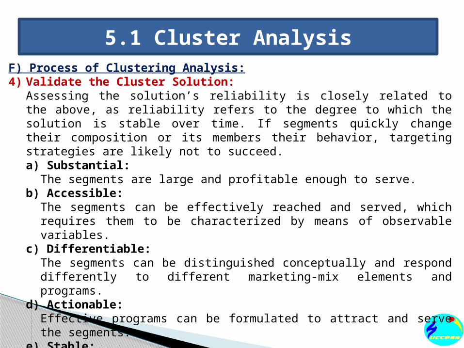
5.1 Cluster AnalysisF) Process of Clustering Analysis:4) Validate the Cluster Solution:

Assessing the solution’s reliability is closely related to the above, as reliability refers to the degree to which the solution is stable over time. If segments quickly change their composition or its members their behavior, targeting strategies are likely not to succeed. a) Substantial:

The segments are large and profitable enough to serve.b) Accessible:

The segments can be effectively reached and served, which requires them to be characterized by means of observable variables.

c) Differentiable:The segments can be distinguished conceptually and respond differently to different marketing-mix elements and programs.

d) Actionable:Effective programs can be formulated to attract and serve the segments.

e) Stable:Only segments that are stable over time can provide the necessary grounds for a successful marketing strategy.

5.1 Cluster AnalysisF) Process of Clustering Analysis:4) Validate the Cluster Solution:f) Parsimonious:

To be managerially meaningful, only a small set of substantial clusters should be identified.

g) Familiar:To ensure management acceptance, the segments composition should be comprehensible.

h) Relevant:Segments should be relevant in respect of the company’s competencies and objectives.

i) Compactness:Segments exhibit a high degree of within-segment homogeneity and between-segment heterogeneity.

j) Compatibility:Segmentation results meet other managerial functions’ requirements.

5) Interpretation of Data:The final step of any cluster analysis is the interpretation of the clusters. Interpreting clusters always involves examining the cluster centroids, which are the clustering variables’ average values of all objects in a certain cluster.

5.1 Cluster AnalysisG) Amalgamation or Linkage Rules:1) Single Linkage (nearest neighbor):

As described above, in this method the distance between two clusters is determined by the distance of the two closest objects (nearest neighbors) in the different clusters. This rule will, in a sense, string objects together to form clusters, and the resulting clusters tend to represent long "chains."

2) Complete Linkage (furthest neighbor):In this method, the distances between clusters are determined by the greatest distance between any two objects in the different clusters (i.e., by the "furthest neighbors"). This method usually performs quite well in cases when the objects actually form naturally distinct "clumps." If the clusters tend to be somehow elongated or of a "chain" type nature, then this method is inappropriate.

3) Un-weighted pair-group Average:In this method, the distance between two clusters is calculated as the average distance between all pairs of objects in the two different clusters. This method is also very efficient when the objects form natural distinct "clumps," however, it performs equally well with elongated, "chain" type clusters.

5.1 Cluster AnalysisG) Amalgamation or Linkage Rules:4) Weighted pair-group Average:

This method is identical to the un-weighted pair-group average method, except that in the computations, the size of the respective clusters (i.e., the number of objects contained in them) is used as a weight. Thus, this method (rather than the previous method) should be used when the cluster sizes are suspected to be greatly uneven. Note that in their book, Sneath and Sokal (1973) introduced the abbreviation WPGMA to refer to this method as weighted pair-group method using arithmetic averages.

5) Un-weighted pair-group Centroid:The centroid of a cluster is the average point in the multidimensional space defined by the dimensions. In a sense, it is the center of gravity for the respective cluster. In this method, the distance between two clusters is determined as the difference between centroids. Sneath and Sokal (1973) use the abbreviation UPGMC to refer to this method as un-weighted pair-group method using the centroid average.

6) Weighted pair-group Centroid (median):This method is identical to the previous one, except that weighting is introduced into the computations to take into consideration differences in cluster sizes (i.e., the number of objects contained in them).

5.1 Cluster AnalysisH) Psychographic Segmentation:Consumers are not all alike. This provides a challenge for the development and marketing of profitable products and services. Not every offering will be right for every customer, nor will every customer be equally responsive to marketing efforts. Segmentation is a way of organizing customers into groups with similar traits, product preferences, or expectations. Once segments are identified, marketing messages and in many cases even products can be customized for each segment. The better the segment(s) chosen for targeting by a particular organization, the more successful the organization is assumed to be in the marketplace. Since its introduction in the late 1950s, market segmentation has become a central concept of marketing practice.Segments are constructed on the basis of customers:a) Demographic characteristics, b) Psychographics, c) Desired benefits from products/services,d) Past-purchase and product-use behaviors.

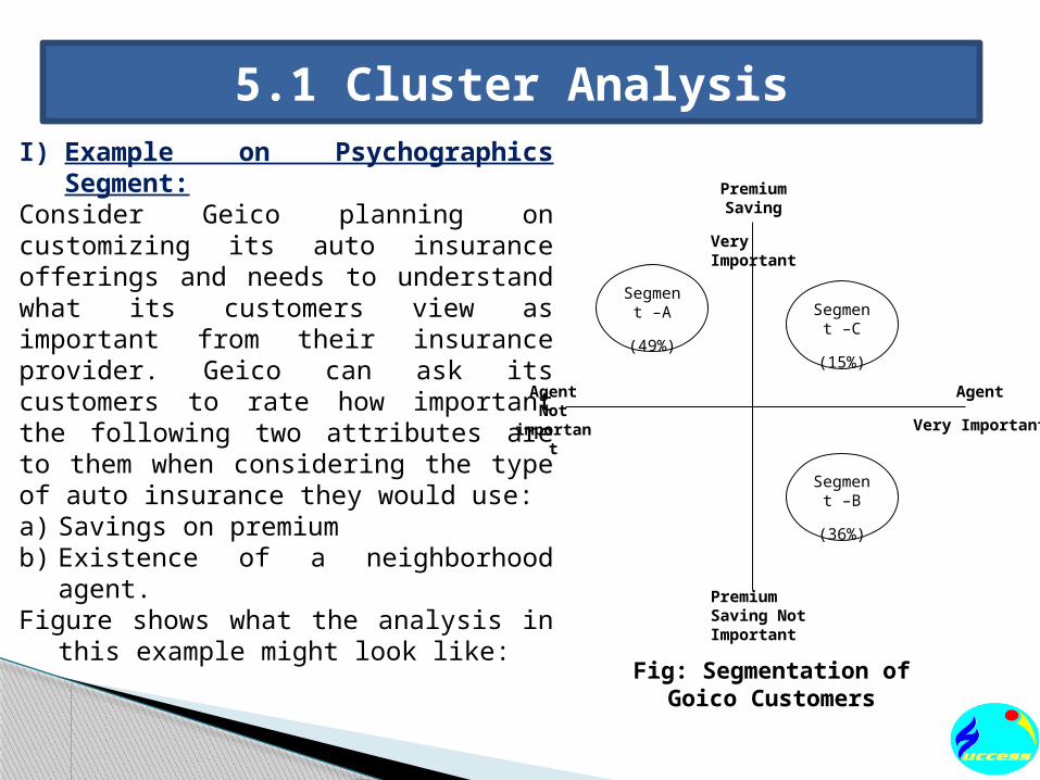
5.1 Cluster AnalysisI) Example on Psychographics Segment:Consider Geico planning on customizing its auto insurance offerings and needs to understand what its customers view as important from their insurance provider. Geico can ask its customers to rate how important the following two attributes are to them when considering the type of auto insurance they would use:a) Savings on premiumb) Existence of a neighborhood agent.Figure shows what the analysis in this example

might look like:

Premium Saving

Very Important

Agent Not important

Premium Saving Not Important

Agent

Very Important

Segment –A

(49%)

Segment –C

(15%)

Segment –B

(36%)

Fig: Segmentation of Goico Customers

5.1 Cluster AnalysisJ) Interpretation of Example:

1) Cluster analysis to interpret data:Cluster analysis is a class of statistical techniques that can be applied to data that exhibits natural groupings. Cluster analysis makes no distinction between dependent and independent variables. The entire set of interdependent relationships is examined. Cluster analysis sorts through the raw data on customers and groups them into clusters. A cluster is a group of relatively homogeneous customers. Customers who belong to the same cluster are similar to each other. They are also dissimilar to customers outside the cluster, particularly customers in other clusters. The primary input for cluster analysis is a measure of similarity between customers, such as

a) correlation coefficients, b) distance measures,c) association coefficients.

5.1 Cluster AnalysisJ) Interpretation of Example:

2) Distance Measures:The main input into any cluster analysis procedure is a measure of distance between individuals who are being clustered. Distance between two individuals is obtained through a measure called “Euclidean distance.” lf two individuals, Joe and Sam, are being clustered on the basis of n variables, then the Euclidean distance between Joe and Sam is represented as: Euclidean=

Where,XJoe, 1 = Respondents the value of Joe along variable 1,XSam, 1 = Respondents the value of Sam along variable 1

2 2,1 .1 , ,( ) ... ( ) Joe Sam Joe n Sam nx x x x

5.1 Cluster AnalysisJ) Interpretation of Example:3) K-Means Clustering Algorithm:

K-means clustering belongs to the non-hierarchical class of clustering aIgorithn1s. It is one of the more popular algorithms used for clustering in practice because of its simplicity and speed. It is considered to be more robust to different types of variables, is more appropriate for large datasets that are common in marketing, and is less sensitive to some customers who are outliers (in other words, extremely different from others).For K-means clustering, the user has to specify the number of clusters required before the clustering algorithm is started. The basic algorithm for K-means clustering is as follows:a) Choose the number of clusters, ‘k’.b) Generate k random points as cluster centroids.c) Assign each point to the nearest cluster centroid.d) Recomputed the new cluster centroid.

Repeat the two previous steps until some convergence criterion is met. Usually the convergence criterion is that the assignment of customers to clusters has not changed over multiple iterations.

5.1 Cluster AnalysisJ) Interpretation of Example:4) Profiling Clusters:

Once clusters are identified, the description of the clusters in terms of the variables used for clustering—or using additional data such as demographics helps in customizing marketing strategy for each segment. This process of describing the clusters is termed “profiling." Figure Iis an example of such a process. A good deal of cluster-analysis software also provides information on which cluster a customer belongs to. This information can be used to calculate the means of the profiling variables for each cluster.

5) Conclusion:Given a segmentation basis, the K—means clustering algorithm would identify clusters and the customers that belong to each cluster. The management, however, has to carefully select the variables to use for segmentation. Criteria frequently used for evaluating the effectiveness of a segmentation scheme include: identifiability, sustainability, accessibility, and action ability dentyiability refers to the extent that managers can recognize segments in the marketplace.

5.2 Multidimensional Scaling:Multidimensional scaling (MDS) is a means of visualizing the level of similarity of individual cases of a dataset. It refers to a set of related ordination techniques used in information visualization, in particular to display the information contained in a distance matrix.

A) Meaning:Multidimensional scaling (MDS) is a series of techniques that helps the analyst to identify key dimensions underlying respondents’ evaluations of objects. It is often used in Marketing to identify key dimensions underlying customer evaluations of products, services or companies.Once the data is in hand, multidimensional scaling can help determine: a) what dimensions respondents use when evaluating objects b) how many dimensions they may use in a particular situation c) the relative importance of each dimension, and d) how the objects are related perceptually

5.2 Multidimensional Scaling:B) Types of Multidimensional Scaling:

Classical multidimen

sional scaling

Metric multidimen

sional scaling

Non-metric multidimen

sional scaling

Generalized multidimen

sional scaling

5.2 Multidimensional Scaling:B) Types of Multidimensional Scaling:1) Classical multidimensional scaling:

It is also known as Principal Coordinates analysis, Torgerson Scaling or Torgerson–Gower scaling.

2) Metric multidimensional scaling:It is a superset of classical MDS that generalizes the optimization procedure to a variety of loss functions and input matrices of known distances with weights and so on.

3) Non-metric multidimensional scaling:In contrast to metric MDS, non-metric MDS finds both a non-parametric monotonic relationship between the dissimilarities in the item-item matrix and the Euclidean distances between items, and the location of each item in the low-dimensional space. The relationship is typically found using isotonic regression.

4) Generalized multidimensional scaling:It is an extension of metric multidimensional scaling, in which the target space is an arbitrary smooth non-Euclidean space. In cases where the dissimilarities are distances on a surface and the target space is another surface, GMDS allows finding the minimum-distortion embedding of one surface into another.

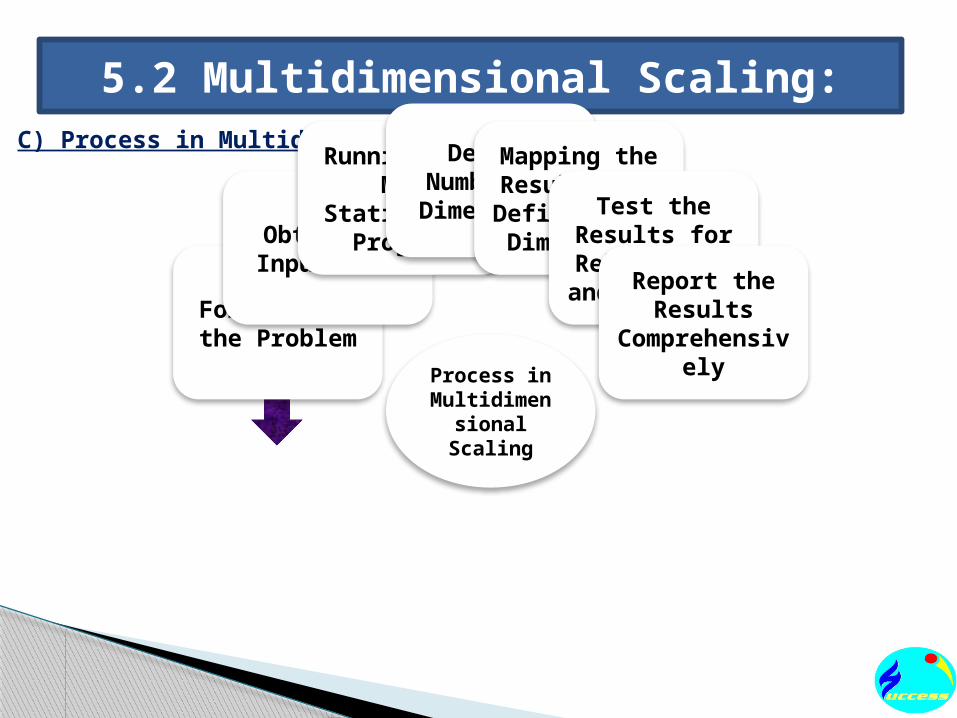
5.2 Multidimensional Scaling:C) Process in Multidimensional Scaling:

Process in Multidime

nsional Scaling

Formulating the Problem

Obtaining Input Data

Running the MDS

Statistical Program

Decide Number of Dimensions

Mapping the Results and Defining the Dimensions

Test the Results for Reliability

and ValidityReport the Results

Comprehensively

5.2 Multidimensional Scaling:C) Process in Multidimensional Scaling: 1) Formulating the Problem:

What variables do you want to compare? How many variables do you want to compare? More than 20 is often considered cumbersome. Fewer than 8 (4 pairs) will not give valid results. What purpose is the study to be used for?

2) Obtaining Input Data:Respondents are asked a series of questions. For each product pair, they are asked to rate similarity (usually on a 7 point Liker scale from very similar to very dissimilar).

3) Running the MDS Statistical Program:Software for running the procedure is available in many software for statistics. Often there is a choice between Metric MDS (which deals with interval or ratio level data), and No metric MDS (which deals with ordinal data).

4) Decide Number of Dimensions:The researcher must decide on the number of dimensions they want the computer to create. The more dimensions, the better the statistical fit, but the more difficult it is to interpret the results.

5.2 Multidimensional Scaling:C) Process in Multidimensional Scaling: 5) Mapping the Results and Defining the Dimensions:

The statistical program (or a related module) will map the results. The map will plot each product (usually in two-dimensional space). The proximity of products to each other indicate either how similar they are or how preferred they are, depending on which approach was used. How the dimensions of the embedding actually correspond to dimensions of system behavior, however, is not necessarily obvious.

6) Test the Results for Reliability and Validity:Compute R-squared to determine what proportion of variance of the scaled data can be accounted for by the MDS procedure. An R-square of 0.6 is considered the minimum acceptable level. An R-square of 0.8 is considered good for metric scaling and .9 is considered good for non-metric scaling.

7) Report the Results Comprehensively:Along with the mapping, at least distance measure (e.g., Sorenson index, Jacquard index) and reliability (e.g., stress value) should be given. It is also very advisable to give the algorithm (e.g., Kruskal, Mather), which is often defined by the program used (sometimes replacing the algorithm report), if you have given a start configuration or had a random choice, the number of runs, the assessment of dimensionality, the Monte Carlo method results, the number of iterations, the assessment of stability, and the proportional variance of each axis (r-square).

5.2 Multidimensional Scaling:D) Scenario Example on Multidimensional Scaling :

We are interested in understanding consumers’ perceptions of six candy bars on the market. Instead of trying to gather information about consumers’ evaluation of the candy bars on a number of attributes, the researcher will instead gather only perceptions of overall similarities or dissimilarities. The data are typically gathered by having respondents give simple global responses to statements such as these:a) Rate the similarity of products A and B on a 10-point scale b) Product A is more similar to B than to C c) I like product A better than product C

Candy Bar A B C D E F

A - 2 13 4 3 8

B 12 6 5 7

C 9 10 11

D - 1 14

E - - 15

F - - -

5.2 Multidimensional Scaling:E) Steps of Multidimensional scaling to solve such problem:

Step 1: Objectives of Multidimensional

Scaling

Step 2: Research Design of MDS

Step 3: Assumptions of Multidimensional Scaling Analysis

Step 4: Deriving the MDS Solution and Assessing Overall Fit

Step 5: Interpreting the MDS Results

Step 6: Validating the MDS Results


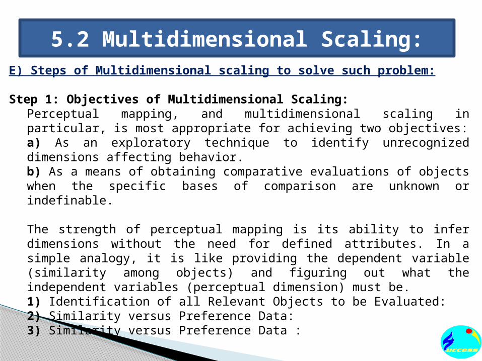
Step 1: Objectives of Multidimensional Scaling:Perceptual mapping, and multidimensional scaling in particular, is most appropriate for achieving two objectives:a) As an exploratory technique to identify unrecognized dimensions affecting behavior.b) As a means of obtaining comparative evaluations of objects when the specific bases of comparison are unknown or indefinable.

The strength of perceptual mapping is its ability to infer dimensions without the need for defined attributes. In a simple analogy, it is like providing the dependent variable (similarity among objects) and figuring out what the independent variables (perceptual dimension) must be.1) Identification of all Relevant Objects to be Evaluated:2) Similarity versus Preference Data:3) Similarity versus Preference Data :


Step 2: Research Design of MDS:Perceptual mapping techniques can be classified by the nature of the responses obtained from the individual concerning the object. 1) Objects: Their Number and Selection:

An implicit assumption in perceptual mapping is that there are common characteristics, either objective or perceived, that the respondent could use for evaluations. Therefore it is vital that the objects be comparable.

2) Collection of Similarity or Preference Data:The primary distinction among multidimensional scaling programs is the type of data (qualitative or quantitative) used to represent similarity and preferences.

3) Similarities Data:When collecting similarities data, the researcher is trying to determine which items are the

most similar to each other and which are the most dissimilar. 4) Preference Data:Preference implies that stimuli should be judged in terms of dominance relationships – that is,

stimuli are ordered in terms of the preference for some property.

5.2 Multidimensional Scaling:E) Steps of Multidimensional scaling to solve such problem:Step 2: Research Design of MDS:5) Similarity Data:

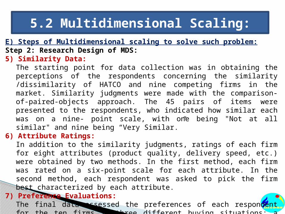
The starting point for data collection was in obtaining the perceptions of the respondents concerning the similarity /dissimilarity of HATCO and nine competing firms in the market. Similarity judgments were made with the comparison-of-paired-objects approach. The 45 pairs of items were presented to the respondents, who indicated how similar each was on a nine- point scale, with one being "Not at all similar" and nine being “Very Similar.”

6) Attribute Ratings:In addition to the similarity judgments, ratings of each firm for eight attributes (product quality, delivery speed, etc.) were obtained by two methods. In the first method, each firm was rated on a six-point scale for each attribute. In the second method, each respondent was asked to pick the firm best characterized by each attribute.

7) Preference Evaluations:The final data assessed the preferences of each respondent for the ten firms in three different buying situations: a straight re-buy, a modified re-buy and a new-buy situation. In each situation, the respondents ranked the firms in order of preference for that particular type of purchase.


Step 3: Assumptions of Multidimensional Scaling Analysis:Multidimensional scaling, while having no restraining assumptions on the methodology, type of data, or form of the relationships among the variables, does require that the researcher accept several tenets about perception, including the following:1) Each respondent will not perceive a stimulus to have the same dimensionality (although it is thought that most people judge in terms of a limited number of characteristics or dimensions). 2) Respondents need not attach the same level of importance to a dimension, even if all respondents perceive this dimension. 3) Judgments of a stimulus in terms of either dimensions or levels of importance need not remain stable over time. People may not maintain the same perceptions for long periods of time.


Step 4: Deriving the MDS Solution and Assessing Overall Fit:

The determination of how many dimensions are actually represented in the data is generally reached through one of three approaches: subjective evaluation, screen plots of the stress measures, or an overall index of fit.

a) Incorporating Preferences into MDS:Up to this point, we have concentrated on developing perceptual maps based on

similarity judgments. However, perceptual maps can also be derived from preferences. A critical assumption is the homogeneity of perception across individuals for the set of objects. This allows all differences to be attributed to preferences, not perceptual differences.


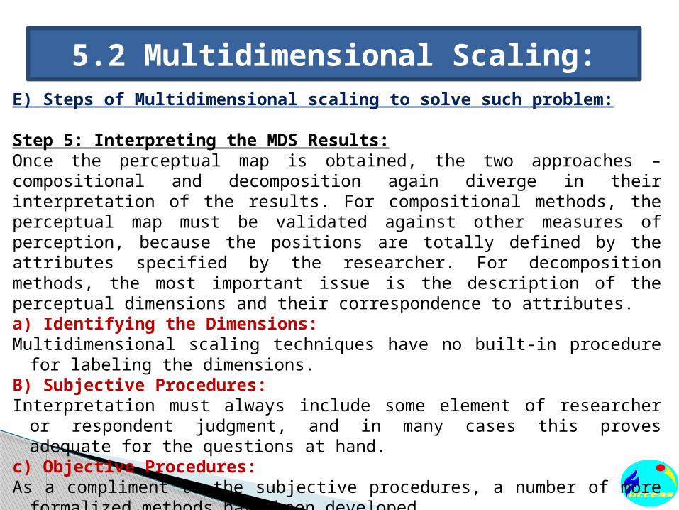
Step 5: Interpreting the MDS Results:Once the perceptual map is obtained, the two approaches – compositional and decomposition again diverge in their interpretation of the results. For compositional methods, the perceptual map must be validated against other measures of perception, because the positions are totally defined by the attributes specified by the researcher. For decomposition methods, the most important issue is the description of the perceptual dimensions and their correspondence to attributes.a) Identifying the Dimensions:Multidimensional scaling techniques have no built-in procedure for labeling the dimensions. B) Subjective Procedures:Interpretation must always include some element of researcher or respondent judgment, and

in many cases this proves adequate for the questions at hand. c) Objective Procedures:As a compliment to the subjective procedures, a number of more formalized methods have

been developed.


Step 6: Validating the MDS Results:The most direct approach towards validation is a split-sample or multi-sample comparison, in which either the original sample is divided or a new sample is collected. Most often the comparison between results is done visually or with a simple correlation of coordinates.a) Correspondence Analysis:

Correspondence Analysis is an interdependence technique that has become increasingly popular for dimension reduction and perceptual mapping. It is a compositional technique because the perceptual map is based on the association between objects and a set of descriptive characteristics or attributes specified by the researcher. Its most direct application is portraying the “correspondence” of categories of variables, which is then used as the basis for developing perceptual maps.

5.3 Perceptual MappingA) Meaning:Perceptual mapping has been used to satisfy marketing and advertising information needs related to product positioning, competitive market structure, consumer preferences and brand perceptions. Perceptual maps satisfy these types of information needs by analyzing and then translating consumers' numeric ratings, brand similarity data and brand preference data into a visual representation of how those consumers view the set of brands and products.

B) Definitions:

1) Kardes, Cronley, & Cline: “Perceptual maps measure the way products are positioned in the minds of consumers and show these perceptions on a graph whose axes are formed by product attributes.”

2) (Ferrell & Hartline, 2008):“A perceptual map represents customer perceptions and preferences spatially by means of a visual display”

5.3 Perceptual MappingC) Approaches to Perceptual Mapping:There are two approaches to perceptual mapping.1) Attribute based perceptual mapping:

Attribute based approaches require a respondent to evaluate a set of brands on a large number of specific attributes, typically those attributes felt to influence how consumers perceive, evaluate and distinguish among brands and products. Attribute based perceptual maps can be created through the use of one of three mathematical techniques: factor analysis, discriminate analysis and correspondence analysis. These approaches to attribute based perceptual mapping are discussed in the next section.

2) Non-attribute based perceptual mapping:Non-attribute based approaches require a respondent to rate brands in terms of similarities or preferences rather than attributes. A discussion of non-attribute based perceptual mapping is presented later. While attribute and non-attribute based approaches to perceptual mapping differ in terms of the types of data collected, both approaches share the fundamental assumption of perceptual maps that consumers use broad dimensions to evaluate brands and products.

5.3 Perceptual MappingD) Information Require to Perceptual Mapping:1) The Number of Dimensions Consumers use to Distinguish between Brands or Products:

This information reveals tl1e complexity of the product category from the consumer's perspective. I-lightly complex categories are those where consumers use a large number of dimensions to evaluate brands and products; less complex categories are typically those where fewer dimensions are used.

2) The Nature and Characteristics of these Dimensions:This information reveals the specific attributes or dimensions that consumers use to distinguish among products.

3) The Location of Actual Brands, as well as the Ideal Brand on these Dimensions:This infom1ation reveals consumers' evaluations of tl1e advertiser's product versus other products and versus the ideal product on dimensions of importance. Further, it makes explicit from the consumers' perspective, a brand's most direct competitors and provides a basis for determining the extent to which future advertising should reinforce or seek to change the brands current positioning.

5.4 Discriminant AnalysisA) Methods under Discriminant Analysis:

Multiple Discrimin

ant Analysis

Linear Discriminant

Analysis

K-NNs Discrimin

ant Analysis

5.4 Discriminant AnalysisA) Methods under Discriminant Analysis:1) Multiple Discriminant Analysis:

MDA is also termed Discriminant Factor Analysis and Canonical Discriminant Analysis. It adopts a similar perspective to PCA: the rows of the data matrix to be examined constitute points in a multidimensional space, as also do the group mean vectors. Discriminating axes are determined in this space, in such a way that optimal separation of the predefined groups is attained.

2) Linear Discriminant Analysis:It is the 2-group case of MDA. It optimally separates two groups, using the Mahalanob is metric or generalized distance. It also gives the same linear separating decision surface as Bayesian maximum likelihood discrimination in the case of equal class covariance matrices.

3) K-NNs Discriminant Analysis:Non-parametric (distribution-free) methods dispense with the need for assumptions regarding the probability density function. They have become very popular especially in the image processing area. The K-NNs method assigns an object of unknown affiliation to the group to which the majority of its K nearest neighbors belongs.

5.4 Discriminant AnalysisB)_Discriminant Function:Discriminant analysis is used to analyze relationships between a non-metric dependent variable and metric or dichotomous independent variables. Discriminant analysis attempts to use the independent variables to distinguish among the groups or categories of the dependent variable. The usefulness of a discriminant model is based upon its accuracy rate, or ability to predict the known group memberships in the categories of the dependent variable.Each function is given a discriminant score to determine how well it predicts group placement.1) Structure Correlation Coefficients:

The correlation between each predictor and the discriminant score of each function. 2) Standardized Coefficients:

Each predictor’s unique contribution to each function, therefore this is a partial correlation. Indicates the relative importance of each predictor in predicting group assignment from each function.

3) Functions at Group Centroids: Mean discriminant scores for each grouping variable are given for each function. The farther apart the means are, the less error there will be in classification.

5.4 Discriminant AnalysisC) Goals to Discriminant FunctionThere are two main goals for discriminant analysis:

1) Discrimination:To construct a classifier to distinguish a set of observations from a known population.

2) Classification:To distribute unlabeled observations into labeled groups with the classifier. The emphasis is on deriving a classifier that can be used to sort new observations into the labeled classes.

D) When to Use Discriminant Analysis:3) Data should be from distinct groups.4) DA is used to interpret group differences.5) DA is used to classify new objects.

5.4 Discriminant AnalysisE) Assumptions in Discriminant analysis:The discriminant model has the following assumptions:1) Multivariate Normality:

Data values are from a normal distribution. We can use a normality test to verify this. However, please note that normal assumptions are usually not "fatal". The resultant significance tests may still be reliable.

2) Equality of variance-covariance within Group:The covariance matrix within each group should be equal. Equality Test of Covariance Matrices can be used to verify it. When in doubt, try re-running the analyses using the Quadratic method, or by adding more observations or excluding one or two groups.

3) Low Multicollinearity of the Variables:When high multicollinearity among two or more variables is present, the discriminant function coefficients will not reliably predict group membership. We can use the pooled within-groups correlation matrix to detect multicollinearity. If there are correlation coefficients larger than 0.8, exclude some variables or use Principle Component Analysis first.

5.4 Discriminant AnalysisF) Steps/ Process in Discriminant analysis:

Preparing Analysis Data

Verifying Assumptions

Selecting Discriminant Methods

Interpreting and Verifying the Results

5.4 Discriminant AnalysisF) Steps/ Process in Discriminant analysis:1) Preparing Analysis Data:

a) Enough Sample Size:As a rule, the sample size of the smallest group should exceed the number of variables. Usually it is best that there should be at least 20 for each variable. While this low sample size may work, it is not encouraged. There should be at least 5 observations for each variable.

b) Independent Random Sample (no outliers):Discriminant analysis requires that the observations are independent of one another, i.e., no repeated measures or matched pairs data. In addition, discriminant analysis is highly sensitive to the inclusion of outliers.

c) Selecting Proper Variables:Suppressor variables should be excluded. We can judge by observing the Univariate ANOVA table.

d) Dividing The Sample:The Classification Summary of Training Data evaluates the observation via discriminant functions derived from the same data. The "error rate" is usually larger when the user evaluates the test data, which is not used for discrminant function estimation.

5.4 Discriminant AnalysisF) Steps/ Process in Discriminant analysis:2) Verifying Assumptions:

The normality test, Equality Test of Covariance Matrices, and pooled within-groups correlation matrix can be used to verify the assumptions. Please see Assumptions for more information.

3) Selecting Discriminant Methods:a) Linear or Quadratic:

The Quadratic Discriminant Analysis (QDA) is like the linear discriminant analysis (LDA) except that the covariance matrix in LDA is identical. If the equality test of covariance matrices fails, QDA should be selected. However, though QDA is more flexible for the covariance matrix than LDA, it has more parameters to estimate.

b) Identifiable prior probabilities:Discriminant analysis assumes that prior probabilities of group membership are identifiable. If group population size is unequal, prior probabilities may differ. If one finds that N for each group in the descriptive statistics table is different, use Proportional to group size for the Pier Probabilities option.

5.4 Discriminant AnalysisG) Two Group Discriminant Analyses:

In the two-group case, discriminant function analysis can also be thought of as (and is analogous to) multiple regression (see Multiple Regression; the two-group discriminant analysis is also called Fisher linear discriminant analysis after Fisher, 1936; computationally all of these approaches are analogous). If we code the two groups in the analysis as 1 and 2, and use that variable as the dependent variable in a multiple regression analysis, then we would get results that are analogous to those we would obtain via Discriminant Analysis. In general, in the two-group case we fit a linear equation of the type:

Group = a + b1*x1 + b2*x2 + ... + Bm*xm

Where a is a constant and b1 through bm are regression coefficients. The interpretation of the results of a two-group problem is straightforward and closely follows the logic of multiple regressions: Those variables with the largest (standardized) regression coefficients are the ones that contribute most to the prediction of group membership.

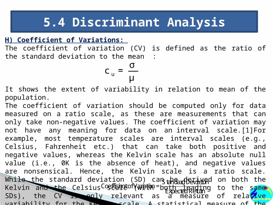
5.4 Discriminant AnalysisH) Coefficient of Variations: The coefficient of variation (CV) is defined as the ratio of the standard deviation to the mean :

It shows the extent of variability in relation to mean of the population.The coefficient of variation should be computed only for data measured on a ratio scale, as these are measurements that can only take non-negative values. The coefficient of variation may not have any meaning for data on an interval scale.[1]For example, most temperature scales are interval scales (e.g., Celsius, Fahrenheit etc.) that can take both positive and negative values, whereas the Kelvin scale has an absolute null value (i.e., 0K is the absence of heat), and negative values are nonsensical. Hence, the Kelvin scale is a ratio scale. While the standard deviation (SD) can be derived on both the Kelvin and the Celsius scale (with both leading to the same SDs), the CV is only relevant as a measure of relative variability for the Kelvin scale. A statistical measure of the dispersion of data points in a data series around the mean. It is calculated as follows:

u

σc =

μ

S tandard DeviationCoefficient of Variation =

Expected Return

pratik meshram-Unit 5 (contemporary mkt r sch)

Education

Transcript of pratik meshram-Unit 5 (contemporary mkt r sch)