PRAM (2) PRAM algorithm design techniques

1PRAM (2)COMP 633 - Prins

COMP 633 - Parallel Computing

Lecture 3 Aug 26, 31 + Sep 2 2021

PRAM (2)PRAM algorithm design techniques

• Reading for next class (Sep 7): PRAM handout secn 5

• Written assignment 1 is posted, due Thu Sep 16


Topics

• PRAM Algorithm design techniques– pointer jumping

– algorithm cascading

– parallel divide and conquer


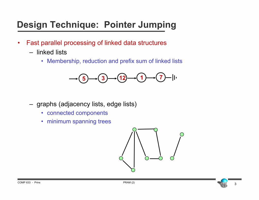
Design Technique: Pointer Jumping

• Fast parallel processing of linked data structures– linked lists

• Membership, reduction and prefix sum of linked lists

– graphs (adjacency lists, edge lists)• connected components• minimum spanning trees

5 3 12 1 7


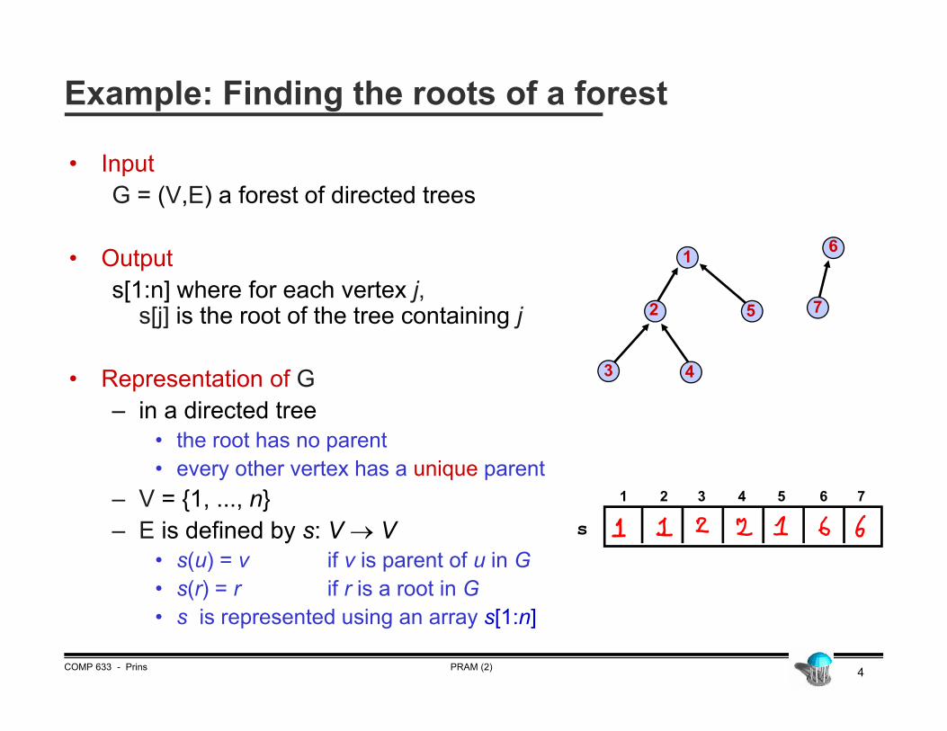
• InputG = (V,E) a forest of directed trees

• Outputs[1:n] where for each vertex j,

s[j] is the root of the tree containing j

• Representation of G– in a directed tree

• the root has no parent• every other vertex has a unique parent

– V = {1, ..., n}– E is defined by s: V V

• s(u) = v if v is parent of u in G• s(r) = r if r is a root in G• s is represented using an array s[1:n]

1

2

3

5

6

7

4

Example: Finding the roots of a forest

s

1 2 3 4 5 6 7


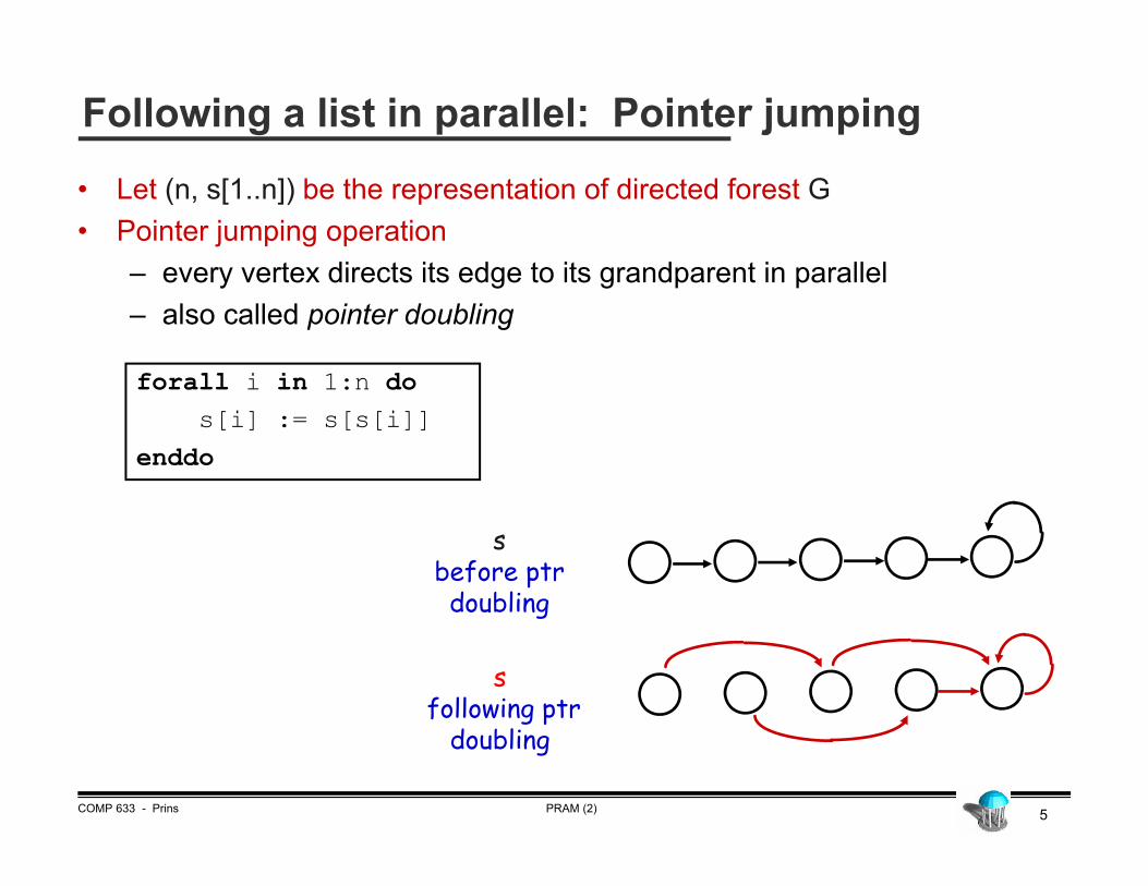
• Let (n, s[1..n]) be the representation of directed forest G• Pointer jumping operation

– every vertex directs its edge to its grandparent in parallel– also called pointer doubling

forall i in 1:n dos[i] := s[s[i]]

enddo

sbefore ptrdoubling

Following a list in parallel: Pointer jumping

sfollowing ptr

doubling


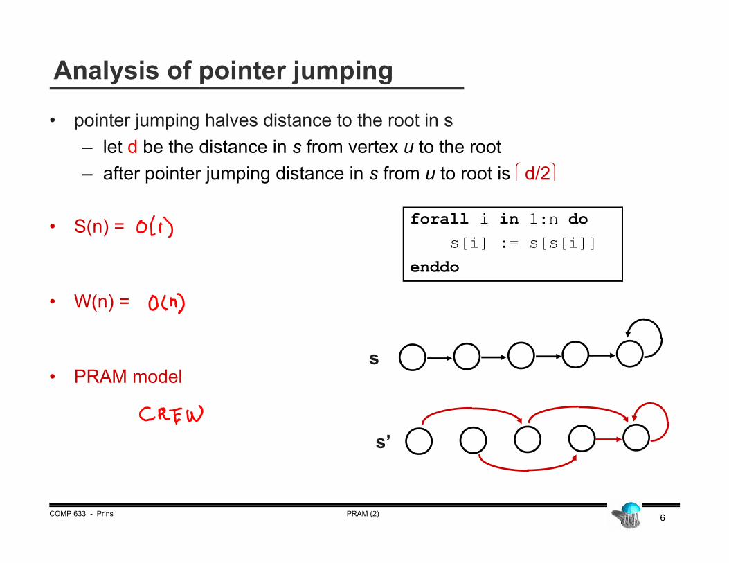
• pointer jumping halves distance to the root in s– let d be the distance in s from vertex u to the root– after pointer jumping distance in s from u to root is d/2

• S(n) =

• W(n) =

• PRAM model

Analysis of pointer jumping

forall i in 1:n dos[i] := s[s[i]]

enddo

s

s’

7

after 1 doubling

after 2 doublings

Initial Forest

Pointer jumping in a forest

All vertices point to the root of their tree

PRAM (2)COMP 633 - Prins


• pointer jumping reaches a fixed point when forest has max height 1– vertex i is distance 1 or less from root when s[i] = s[s[i]]

• forest height 1 s[i] = root of tree containing i

Finding roots of a forest

forall i in 1:n dowhile s[i] != s[s[i]] do

s[i] := s[s[i]]end do

enddo


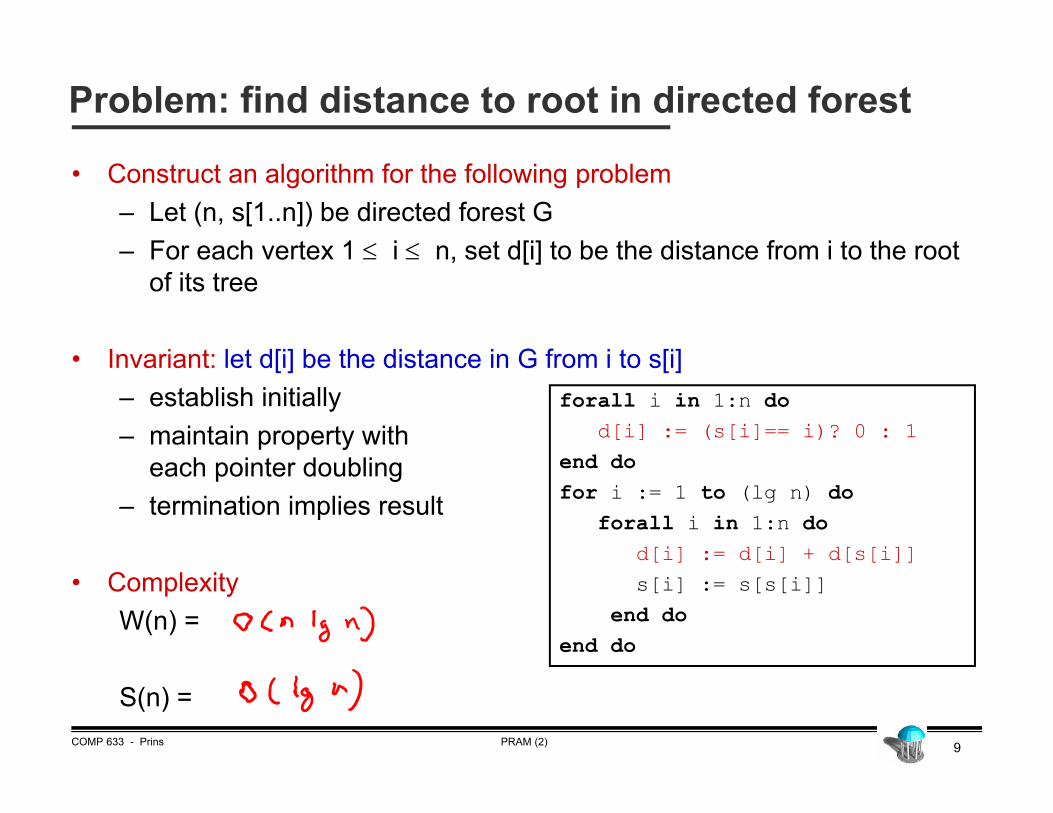
Problem: find distance to root in directed forest

• Construct an algorithm for the following problem– Let (n, s[1..n]) be directed forest G– For each vertex 1 i n, set d[i] to be the distance from i to the root

of its tree

• Invariant: let d[i] be the distance in G from i to s[i]– establish initially– maintain property with

each pointer doubling– termination implies result

• Complexity W(n) =

S(n) =

forall i in 1:n dod[i] := (s[i]== i)? 0 : 1

end dofor i := 1 to (lg n) do

forall i in 1:n dod[i] := d[i] + d[s[i]]s[i] := s[s[i]]

end doend do


Design Technique: Algorithm Cascading

• Technique for improving work efficiency of an algorithm– suppose we have

• work-inefficient but fast parallel algorithm A• work-efficient but slow algorithm B (typically sequential)

– combine (“cascade”) A and B to get best of both

“Speeding up by slowing down”


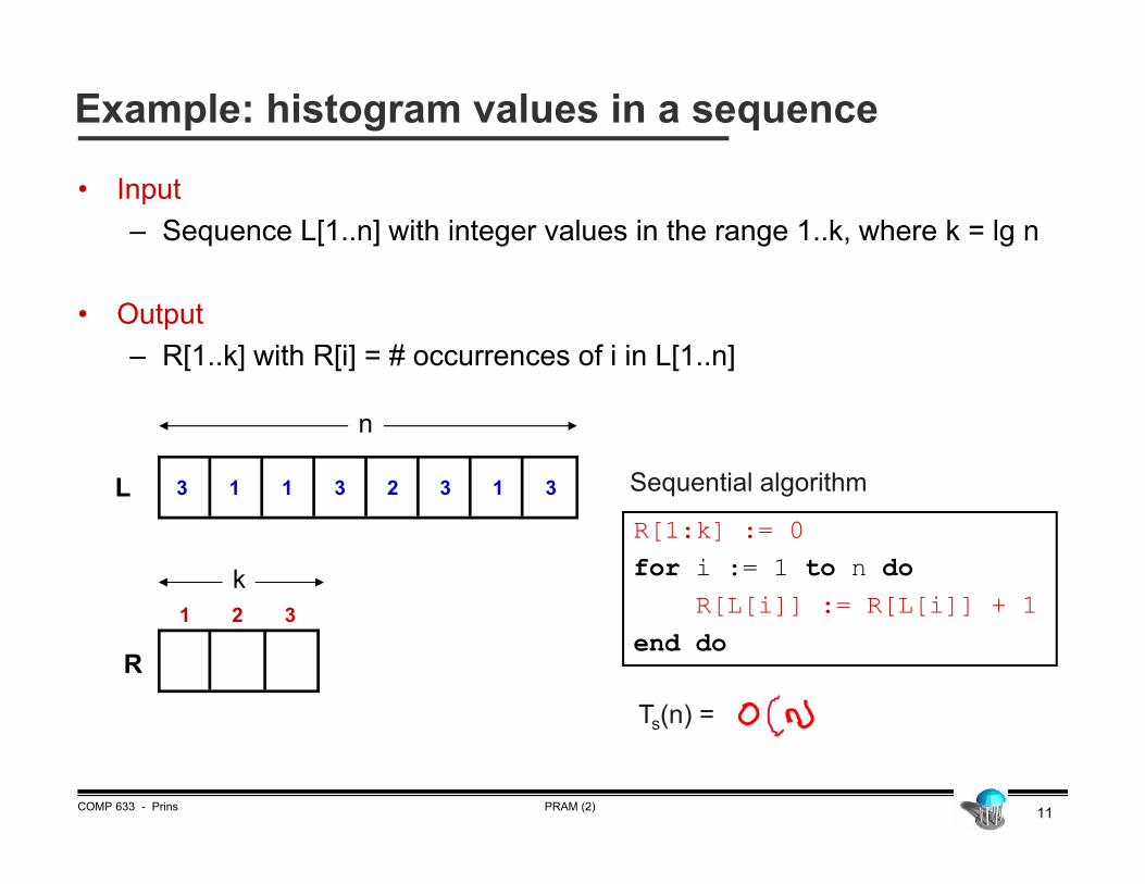
Example: histogram values in a sequence

• Input– Sequence L[1..n] with integer values in the range 1..k, where k = lg n

• Output – R[1..k] with R[i] = # occurrences of i in L[1..n]

R[1:k] := 0for i := 1 to n do

R[L[i]] := R[L[i]] + 1

end do

Sequential algorithm3 1 1 3 2 3 31

1 2 3

L

R

Ts(n) =

n

k


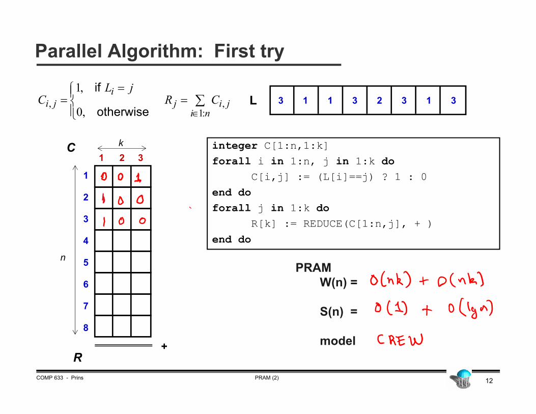
integer C[1:n,1:k]forall i in 1:n, j in 1:k do

C[i,j] := (L[i]==j) ? 1 : 0end doforall j in 1:k do

R[k] := REDUCE(C[1:n,j], + )

end do

PRAMW(n) =

S(n) =

model

Parallel Algorithm: First try

ni

jiji

ji CRjL

C:1

,,,0

,1

otherwise

if

1 2 3k

n

1

2

3

4

5

6

7

8

+

C

R

3 1 1 3 2 3 31L


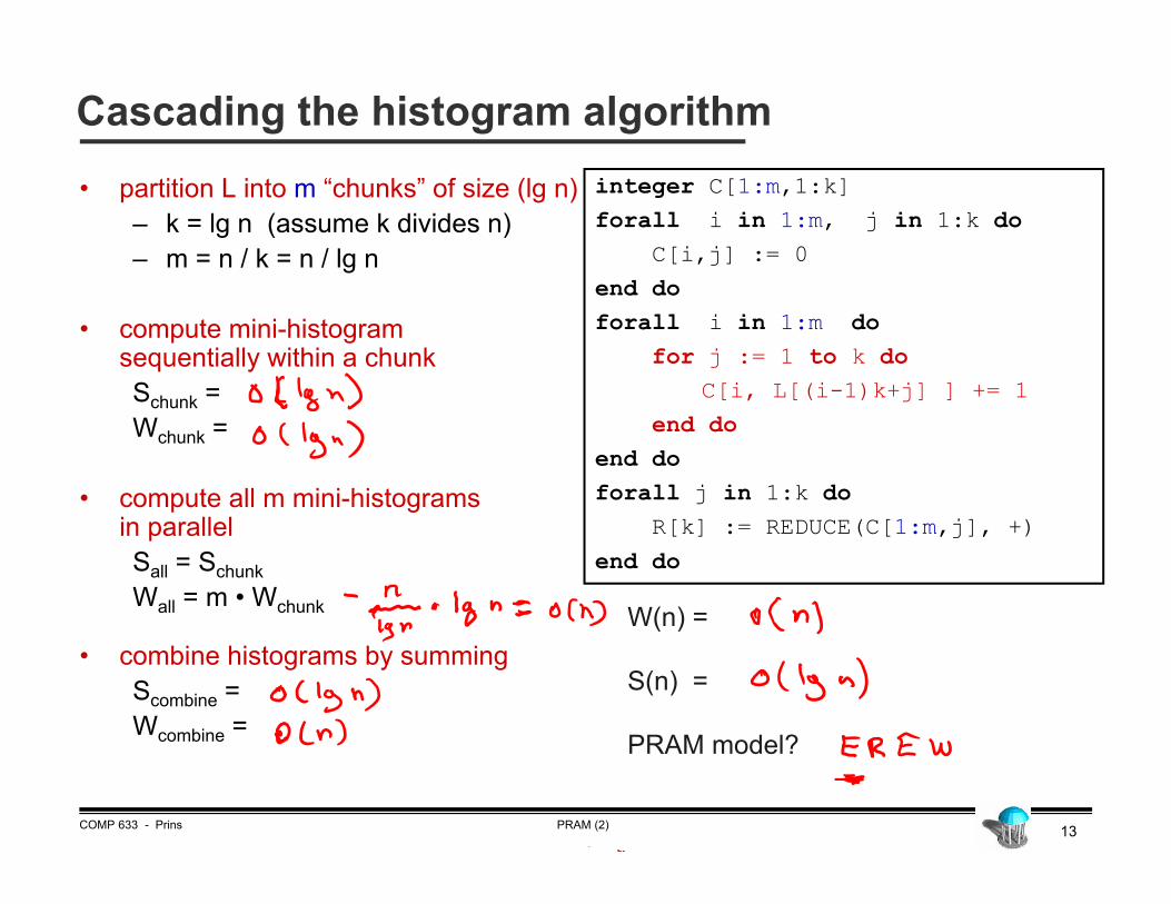
integer C[1:m,1:k]forall i in 1:m, j in 1:k do

C[i,j] := 0end doforall i in 1:m do

for j := 1 to k doC[i, L[(i-1)k+j] ] += 1

end doend doforall j in 1:k do

R[k] := REDUCE(C[1:m,j], +)

end do

Cascading the histogram algorithm• partition L into m “chunks” of size (lg n)

– k = lg n (assume k divides n)– m = n / k = n / lg n

• compute mini-histogramsequentially within a chunk Schunk =Wchunk =

• compute all m mini-histograms in parallelSall = SchunkWall = m • Wchunk

• combine histograms by summingScombine =Wcombine =

W(n) =

S(n) =

PRAM model?


Parallel Divide and Conquer

• To solve problem instance P using parallel divide-and-conquer– divide P into subproblems (possibly in parallel)– apply D&C recursively to each subproblem in parallel– combine subsolutions to produce solution (possibly in parallel)

• Example: sorting– mergesort

• combining– subproblems: left/right half of array– sort each subproblem– merge results

– quicksort• partitioning

– subproblems: values less than pivot, values greater than or equal to pivot– sort each subproblem– concatenate results


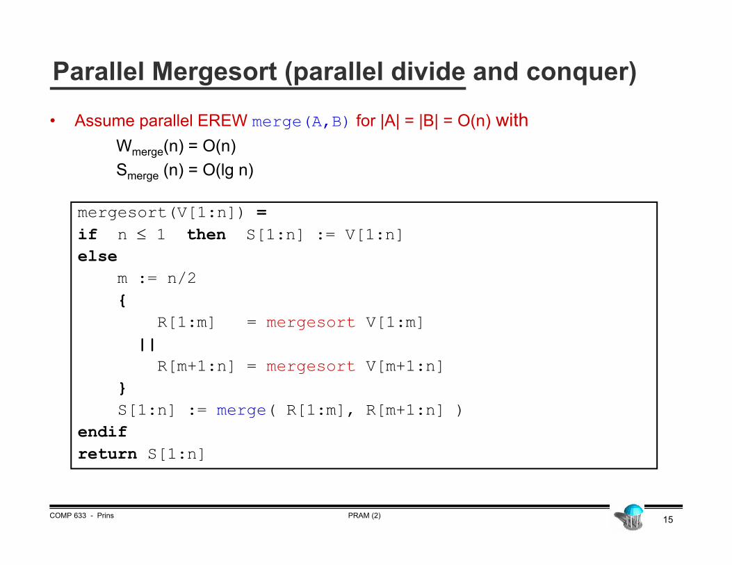
Parallel Mergesort (parallel divide and conquer)• Assume parallel EREW merge(A,B) for |A| = |B| = O(n) with

Wmerge(n) = O(n)Smerge (n) = O(lg n)

mergesort(V[1:n]) =if n 1 then S[1:n] := V[1:n]else

m := n/2{

R[1:m] = mergesort V[1:m] || R[m+1:n] = mergesort V[m+1:n]

}S[1:n] := merge( R[1:m], R[m+1:n] )

endifreturn S[1:n]

16

Mergesort complexity (figure)



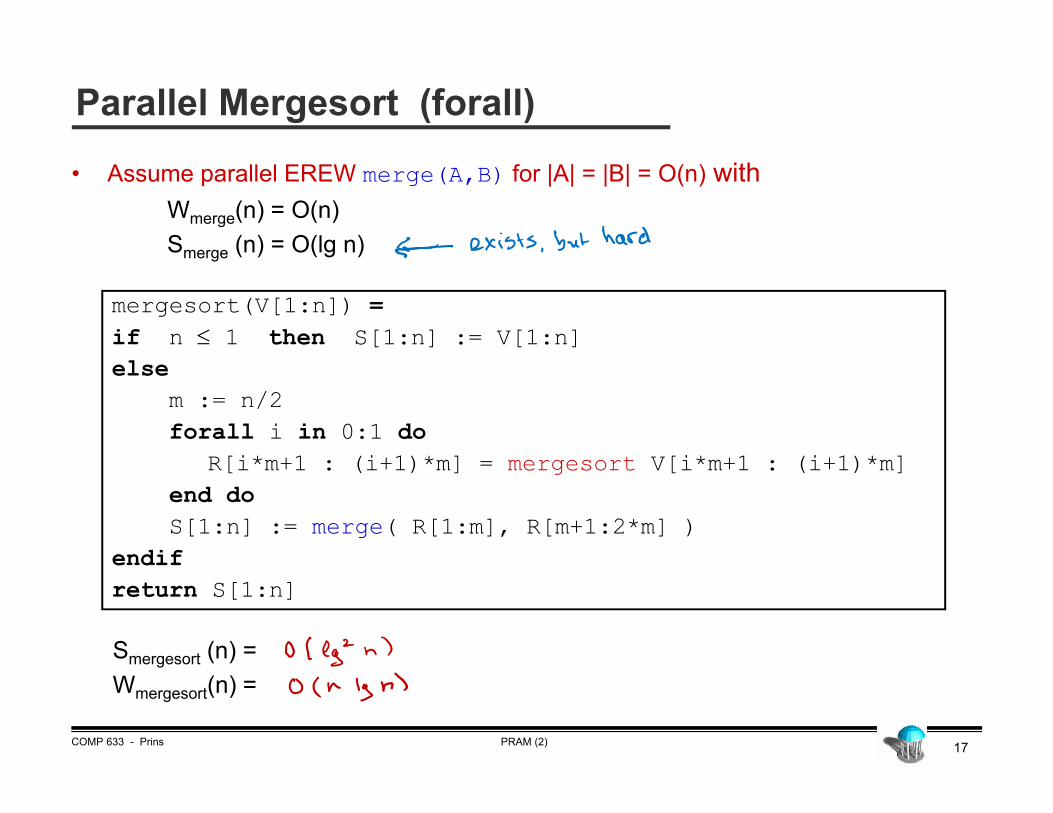
Parallel Mergesort (forall)

mergesort(V[1:n]) =if n 1 then S[1:n] := V[1:n]else

m := n/2forall i in 0:1 do

R[i*m+1 : (i+1)*m] = mergesort V[i*m+1 : (i+1)*m]end doS[1:n] := merge( R[1:m], R[m+1:2*m] )

endifreturn S[1:n]

• Assume parallel EREW merge(A,B) for |A| = |B| = O(n) withWmerge(n) = O(n)Smerge (n) = O(lg n)

Smergesort (n) = Wmergesort(n) =


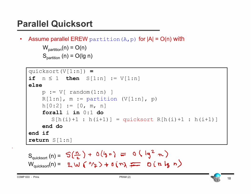
Parallel Quicksort

quicksort(V[1:n]) =if n 1 then S[1:n] := V[1:n]else

p := V[ random(1:n) ]R[1:n], m := partition (V[1:n], p)h[0:2] := [0, m, n]forall i in 0:1 do

S[h(i)+1 : h(i+1)] = quicksort R[h(i)+1 : h(i+1)]end do

end ifreturn S[1:n]

• Assume parallel EREW partition(A,p) for |A| = O(n) withWpartition(n) = O(n)Spartition (n) = O(lg n)

Squicksort (n) = Wquicksort(n) =

19

Quicksort complexity (figure)


Best case: W(n) = 2W(n/2)+O(n) W(n)=O(𝑛 lg 𝑛)S(n) = S(n/2) + O(lg n) S(n)=O(lg 𝑛)

General case: unpredictable number and size of subproblems

Worst case: W n 𝑂 𝑛 , 𝑆 𝑛 𝑂 𝑛 lg𝑛


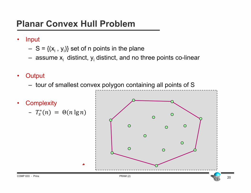
Planar Convex Hull Problem• Input

– S = {(xi , yi)} set of n points in the plane– assume xi distinct, yi distinct, and no three points co-linear

• Output– tour of smallest convex polygon containing all points of S

• Complexity– 𝑇∗ 𝑛 Θ 𝑛 lg 𝑛


Two Parallel Algorithms for Planar Convex Hull

• two divide and conquer algorithms– combining approach– partitioning approach

• combining algorithm (like mergesort)– assume input points presented in order of increasing x coordinate

• can be obtained using 𝑂 𝑛 lg 𝑛 work, 𝑂 lg 𝑛 step sorting algorithm– optimal worst case performance

• partitioning algorithm (like quicksort)– no assumptions about order of input points– suboptimal worst case performance– very good expected case performance


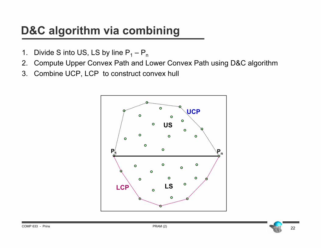
D&C algorithm via combining

1. Divide S into US, LS by line P1 – Pn

2. Compute Upper Convex Path and Lower Convex Path using D&C algorithm3. Combine UCP, LCP to construct convex hull

P1 Pn

US

LS

UCP

LCP


Construction of upper convex path

Divide Recur

Combine (1): find upper common tangent Combine (2): create upper convex path

P1 PnPn/2

Pn/2+1


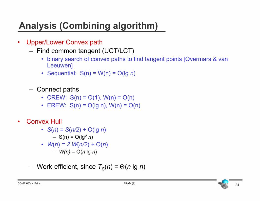
Analysis (Combining algorithm)• Upper/Lower Convex path

– Find common tangent (UCT/LCT) • binary search of convex paths to find tangent points [Overmars & van

Leeuwen]• Sequential: S(n) = W(n) = O(lg n)

– Connect paths• CREW: S(n) = O(1), W(n) = O(n)• EREW: S(n) = O(lg n), W(n) = O(n)

• Convex Hull• S(n) = S(n/2) + O(lg n)

– S(n) = O(lg2 n)• W(n) = 2 W(n/2) + O(n)

– W(n) = O(n lg n)

– Work-efficient, since TS(n) = (n lg n)


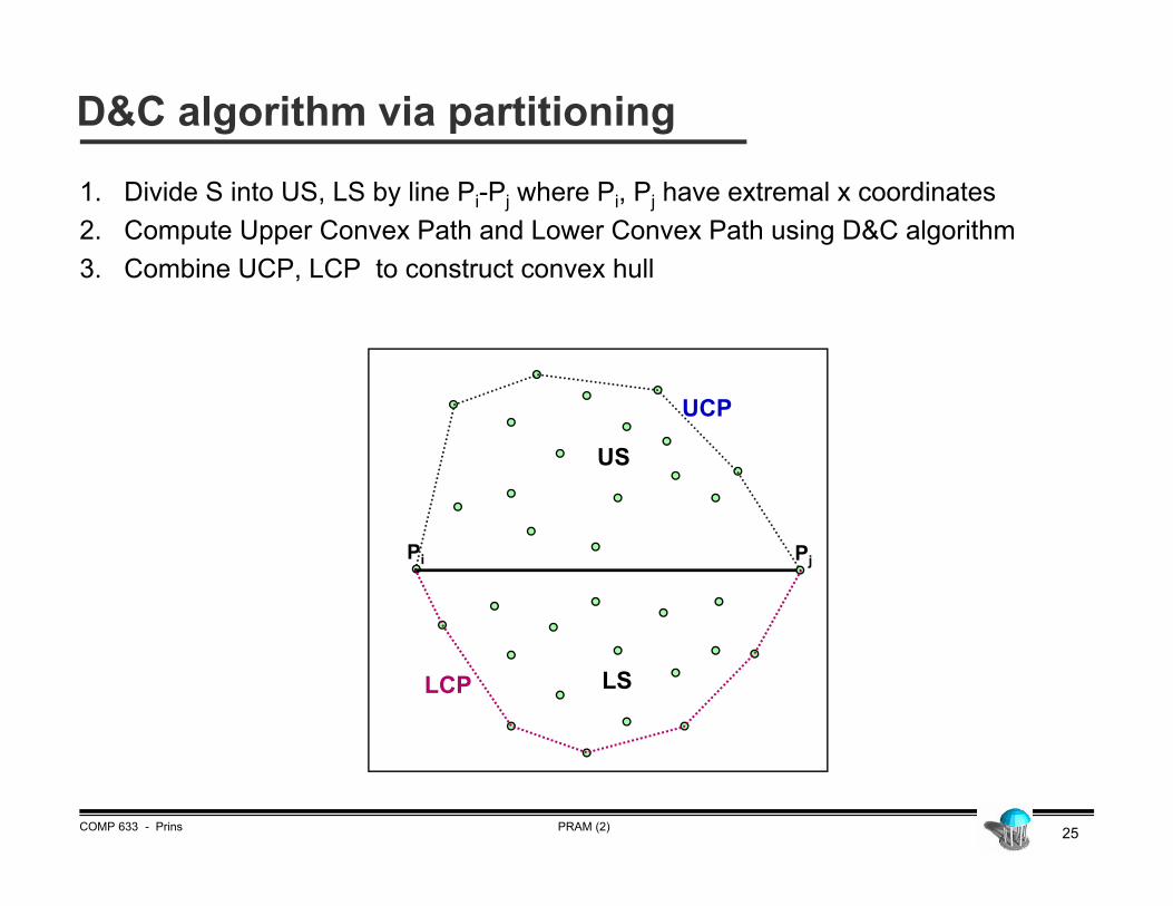
D&C algorithm via partitioning

1. Divide S into US, LS by line Pi-Pj where Pi, Pj have extremal x coordinates2. Compute Upper Convex Path and Lower Convex Path using D&C algorithm3. Combine UCP, LCP to construct convex hull

Pi Pj

US

LS

UCP

LCP


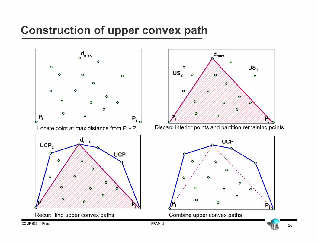
Construction of upper convex path

Locate point at max distance from Pi - Pj Discard interior points and partition remaining points

Recur: find upper convex paths Combine upper convex paths

Pi Pj

dmax

Pi Pj

dmax

Pi Pj

dmax

US1US2

UCP1

UCP2

Pi Pj

UCP


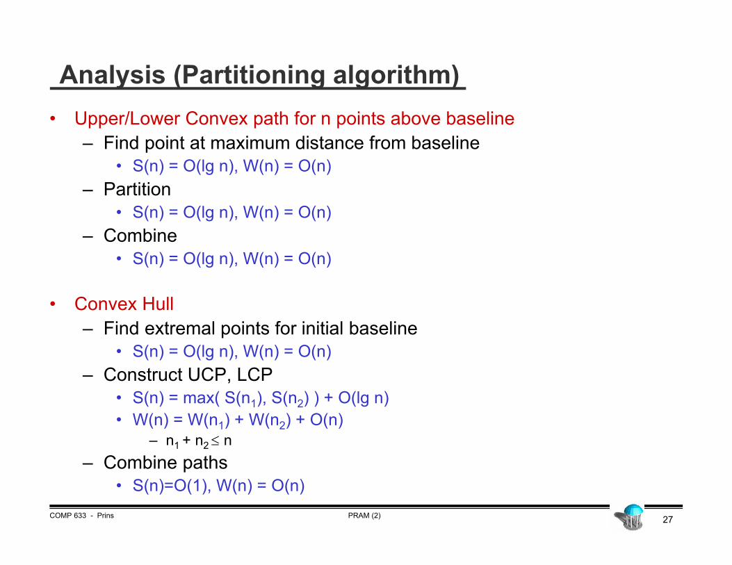
Analysis (Partitioning algorithm)• Upper/Lower Convex path for n points above baseline

– Find point at maximum distance from baseline • S(n) = O(lg n), W(n) = O(n)

– Partition• S(n) = O(lg n), W(n) = O(n)

– Combine• S(n) = O(lg n), W(n) = O(n)

• Convex Hull– Find extremal points for initial baseline

• S(n) = O(lg n), W(n) = O(n)– Construct UCP, LCP

• S(n) = max( S(n1), S(n2) ) + O(lg n)• W(n) = W(n1) + W(n2) + O(n)

– n1 + n2 n– Combine paths

• S(n)=O(1), W(n) = O(n)


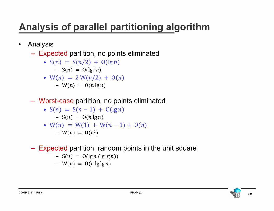
Analysis of parallel partitioning algorithm• Analysis

– Expected partition, no points eliminated• S 𝑛 S 𝑛/2 O lg 𝑛

– S 𝑛 O lg2 𝑛• W 𝑛 2 W 𝑛/2 O 𝑛

– W 𝑛 O 𝑛 lg 𝑛

– Worst-case partition, no points eliminated• S 𝑛 S 𝑛 1 O lg 𝑛

– S 𝑛 O 𝑛 lg 𝑛• W 𝑛 W 1 W 𝑛 1 O 𝑛

– W 𝑛 O 𝑛2

– Expected partition, random points in the unit square– S 𝑛 O lg 𝑛 lg lg 𝑛– W 𝑛 O 𝑛 lg lg 𝑛


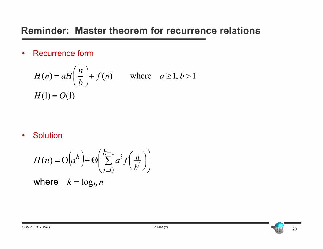
Reminder: Master theorem for recurrence relations

• Recurrence form

• Solution

)1()1(

1,1where)()(

OH

banfbnaHnH

nk

faanH

b

bn

k

i

iki

log

)(1

0

where


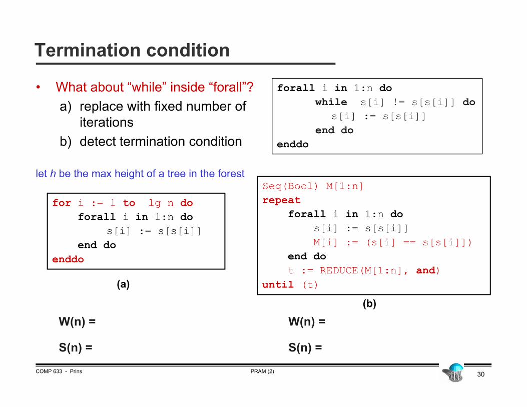
Termination condition

• What about “while” inside “forall”?a) replace with fixed number of

iterationsb) detect termination condition

let h be the max height of a tree in the forest

forall i in 1:n dowhile s[i] != s[s[i]] do


enddo

for i := 1 to lg n doforall i in 1:n do


enddo

Seq(Bool) M[1:n]repeat

forall i in 1:n dos[i] := s[s[i]]M[i] := (s[i] == s[s[i]])

end dot := REDUCE(M[1:n], and)

until (t)

W(n) =

S(n) =

W(n) =

S(n) =

(a)

(b)

PRAM (2) PRAM algorithm design techniques

Documents

Transcript of PRAM (2) PRAM algorithm design techniques