Prairie Hydrological Model Study Progress Report, December 2008

Centre for Hydrology Report No. 4 Revised Version

J. Pomeroy, C. Westbrook, X. Fang, T. Brown, A. Minke, X. Guo Centre for Hydrology

University of Saskatchewan 117 Science Place

Saskatoon, SK S7N 5C8

January 15, 2009

Prairie Hydrological Model Study Progress Report, December 2008

J. Pomeroy, C. Westbrook, X. Fang, T. Brown, A. Minke, X. Guo

Centre for Hydrology University of Saskatchewan

117 Science Place Saskatoon, SK

S7N 5C8 This report is an update on progress made to the middle of December 2008, corresponding to “Milestone Month 20”. According to our study plan, at this milestone “we will have completed a wetland module and with evaluation on Smith Creek Research Basin and archival data available at the Centre for Hydrology (Objective 3, 4)”. More specifically, Objectives 3 and 4 are stated as:

• Objective 3: A physically based, hydrological response unit-based hydrological model, (the Prairie Hydrological Model), will be developed that is suitable for multiple season simulation of the hydrology of the Canadian Prairie environment. The model will be capable of predicting water balance, soil moisture, snow cover, actual evaporation and streamflow on a daily time-step with minimal calibration of model parameters from streamflow records. The model will contain a wetland module that includes assigned variable drainage rates from the wetland. The intended basins would drain to a stream or internally drained lake/wetland, with basin size to be greater than ~1 km2 and less than ~250 km2.

• Objective 4: The Prairie Hydrological Model will be evaluated at Smith Creek through hydrological simulation and quantitative analysis of multi-objective criteria, including streamflow and wetland extent. Whilst calibration will be minimised and limited to non-physical aspects of the model, certain parameters will be optimised from these comparisons. For streamflow, both annual and peak flows are parameters of interest. For wetlands, seasonal extent is the parameter of interest.

Outlined below are the research activities regarding these two objectives, beginning with a description of the model created with the Cold Regions Hydrological Modelling Platform (CRHM), the CRHM-Prairie Hydrological Model, or CRHM-PHM, followed by a description of the addition of the wetland module, and concluding with preliminary results from CRHM-PHM evaluations at Smith Creek. 1. CRHM-PHM Description CRHM-PHM has been developed using the original Cold Regions Hydrological Model (CHRM) platform (Pomeroy et al., 2007a). CRHM is a state-of-the-art, physically based hydrological model which uses a modular, object-oriented structure. Within CRHM, component modules represent basin descriptions, observations or physically based algorithms for calculating hydrological processes, including redistribution of snow by wind, snowmelt, infiltration, evaporation, soil moisture balance, and runoff routing.

1

2

These processes are simulated on landscape units called hydrological response units (HRU). HRUs are defined as spatial units of mass and energy balance calculation corresponding to biophysical landscape units, within which processes and states are represented by single sets of parameters, state variables, and fluxes. HRUs can be finely scaled (hillslope segment), or coarsely scaled (sub-basin). HRUs in the prairies typically correspond to agricultural fields (stubble or fallow fields), natural cover (grassland or forest woodland), and bodies of water (lake or pond) (Fang and Pomeroy, 2008). CRHM has shown good simulations in a semi-arid, well-drained prairie basin (Fang and Pomeroy, 2007), boreal and arctic basins (Pomeroy et al., 2007a) and in a sub-humid, poorly and internally drained prairie basin (Fang and Pomeroy, 2008). For modelling large basins (greater than 250 km2), CRHM has a new component feature called “Group”, in which sequential, physically based modules are linked together and applied to all HRUs. A new large basin modelling feature that uses Groups is the representative basins (RB), in which a set of physically based modules are assembled with certain arrangement of HRUs to represent a sub-basin type (RB) that occurs frequently. Streamflow output from a number of RBs are then routed along the main stream through lakes, wetlands and channel. In this way, CRHM is capable of modelling a large basin such as Smith Creek (~445 km2) by dividing it into several sub-basins. To develop a prairie hydrological model that is suitable for a basin with a large number of wetland drainage networks, a new wetland module was incorporated into CRHM-PHM, which is described in the following section. 2. Wetland Module Description A new wetland module was developed by modifying a soil moisture balance model, which calculates soil moisture balance and drainage (Dornes et al., 2008). This model was modified from an original soil moisture balance routine developed by Leavesley et al., (1983). The changes are to make this algorithm more consistent with what is known about prairie water storage and drainage (Pomeroy et al., 2007b). A flowchart of the wetland module is shown in Figure 1. The soil moisture balance model divides the soil column into two layers; the top layer is called the recharge zone. Inputs to the soil column layers are derived from infiltration from both snowmelt and rainfall. Evapotranspiration withdraws moisture from both soil column layers. Evaporation only occurs from the recharge zone, and water for transpiration is taken out of the entire soil column. Excess water from both soil column layers satisfies groundwater flow requirements before being discharged to subsurface flow (representing flow in macropores that occurs in cracking clay, very coarse soils and in organic soils). The movement of runoff, subsurface discharge and groundwater discharge between HRUs is calculated by a routing module. Two new components - depression and pond - were added to the soil moisture balance model to model wetland drainage. Depressional storage represents small scale (sub-HRU) transient water storage on the surface of fields, pastures and woodlands. Pond storage represents water storage that dominates a HRU in wet conditions, though the pond can be permitted to dry up in drought conditions. The inputs to depressional storage are from surface runoff and overland flow after the soil column is saturated. After the depressional storage is filled, overland flow is generated via the fill-and-spill process (Spence and Hosler, 2007), in which over-topping of the

3

Figure 1. CRHM-PHM wetland module flowchart.

depression results in runoff but minimal leakage of water from the depression to sub-surface storage is permitted before it overtops. Evaporation is permitted from depressional storage. Pond storage works in a similar manner to depressional storage, except that the pond area does not have a soil column, and inputs are derived from uphill surface runoff and infiltration. In the wetland module, both depressions and ponds have storage capacity; the difference is that depressional storage represents ephemeral wetlands or drained wetlands on cultivated fields, whilst pond storage characterizes a large permanent or non-drained wetland or lake. This wetland modelling scheme provides the flexibility to allow CRHM-PHM to model wetland drainage factors (drained vs. non-drained) as well as storage types (temporary vs. permanent). There are a number of key parameters that control the wetland module: antecedent moisture content in the soil column, maximum soil moisture capacity in the soil column, subsurface and groundwater drainage factors, and depression and pond storage capacity. Values for antecedent soil moisture content were determined based on gravimetric measurement of soil samples taken in the fall of 2007. The maximum soil moisture capacity was related to the depth of rooting zone and to soil texture and was set as the product of rooting depth multiplied by the soil porosity. Subsurface and groundwater drainage factors are the rate of excess water entering groundwater from either the soil column, depression or pond, and the rate of discharge as lateral shallow subsurface and groundwater flows. These rates are very slow compared to the fast rates of surface runoff discharge; hydraulic conductivity based on soil texture was used to estimate these rates. Pond storage capacity was determined from an existing surface area-volume relationship for prairie wetlands; the relationship was derived from a number of wetlands with various sizes in the upper Assiniboine River basin in eastern Saskatchewan (Wiens, 2001). The wetland area of Smith Creek was acquired from the DUC wetland inventory, and wetland volume was estimated by applying the area-volume relationship. Depressional storage was found to be small compared to pond storage. Therefore, small values were provisionally assigned to the depressional storage, noting some uncertainty in the values. The uncertainty could be minimized by using fine resolution DEM derived from LiDAR, which could provide a new way to quantify small depressional storage volumes using a revised volume-area relationship once it is fully confirmed (Hayashi and van der Kamp, 2000). 3. Evaluation of CRHM-PHM with Wetland Module 3.1 Meteorological and field observation dataset The dataset used to drive the CRHM-PHM was collected from the main University of Saskatchewan meteorological station in Smith Creek (SC-1). The dataset includes air temperature (ºC), relative humidity (%), vapour pressure (kPa), wind speed (m/s), precipitation (mm), and radiation (W/m2: incident short-wave, reflected short-wave, and net all-wave). Some of this data is available online http://128.233.99.232/. It should be noted that the vapour pressure is calculated from air temperature and relative humidity. Quality control was conducted to ensure continuity and reduce errors in the dataset. A few data gaps were caused by power outages at the weather station and missing data were

4

Figure 2. Meteorological data at Smith Creek SC-1 station: (a) air temperature (b) relative humidity (c) vapour pressure (d) wind speed (e) cumulative rainfall and snowfall (f) incident and reflected short-wave and net all-wave radiation.

5

Figure 2. Concluded.

6

7

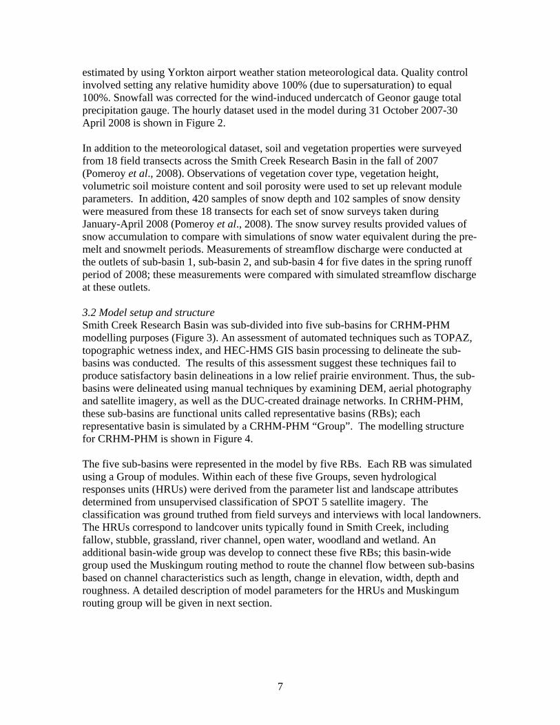
estimated by using Yorkton airport weather station meteorological data. Quality control involved setting any relative humidity above 100% (due to supersaturation) to equal 100%. Snowfall was corrected for the wind-induced undercatch of Geonor gauge total precipitation gauge. The hourly dataset used in the model during 31 October 2007-30 April 2008 is shown in Figure 2. In addition to the meteorological dataset, soil and vegetation properties were surveyed from 18 field transects across the Smith Creek Research Basin in the fall of 2007 (Pomeroy et al., 2008). Observations of vegetation cover type, vegetation height, volumetric soil moisture content and soil porosity were used to set up relevant module parameters. In addition, 420 samples of snow depth and 102 samples of snow density were measured from these 18 transects for each set of snow surveys taken during January-April 2008 (Pomeroy et al., 2008). The snow survey results provided values of snow accumulation to compare with simulations of snow water equivalent during the pre-melt and snowmelt periods. Measurements of streamflow discharge were conducted at the outlets of sub-basin 1, sub-basin 2, and sub-basin 4 for five dates in the spring runoff period of 2008; these measurements were compared with simulated streamflow discharge at these outlets. 3.2 Model setup and structure Smith Creek Research Basin was sub-divided into five sub-basins for CRHM-PHM modelling purposes (Figure 3). An assessment of automated techniques such as TOPAZ, topographic wetness index, and HEC-HMS GIS basin processing to delineate the sub-basins was conducted. The results of this assessment suggest these techniques fail to produce satisfactory basin delineations in a low relief prairie environment. Thus, the sub-basins were delineated using manual techniques by examining DEM, aerial photography and satellite imagery, as well as the DUC-created drainage networks. In CRHM-PHM, these sub-basins are functional units called representative basins (RBs); each representative basin is simulated by a CRHM-PHM “Group”. The modelling structure for CRHM-PHM is shown in Figure 4. The five sub-basins were represented in the model by five RBs. Each RB was simulated using a Group of modules. Within each of these five Groups, seven hydrological responses units (HRUs) were derived from the parameter list and landscape attributes determined from unsupervised classification of SPOT 5 satellite imagery. The classification was ground truthed from field surveys and interviews with local landowners. The HRUs correspond to landcover units typically found in Smith Creek, including fallow, stubble, grassland, river channel, open water, woodland and wetland. An additional basin-wide group was develop to connect these five RBs; this basin-wide group used the Muskingum routing method to route the channel flow between sub-basins based on channel characteristics such as length, change in elevation, width, depth and roughness. A detailed description of model parameters for the HRUs and Muskingum routing group will be given in next section.

8

Figure 3. Map of Smith Creek sub-basin current (2000) drainage network.

Figure 4. CRHM-PHM modelling structure. Each sub-basin is a Representative Basin that is simulated using a Group of modules. Group 6 links the Representative Basins into the Smith Creek Basin for calculation of streamflow at the outlet.

9

10

A set of physically based modules was assembled in each RB Group to simulate the hydrological processes relevant to Smith Creek Research Basin. The schematic of these modules is shown in Figure 5. These modules include:

• observation module – reads the meteorological data (temperature, wind speed, relative humidity, vapour pressure, precipitation, and radiation), providing these inputs to other modules;

• Garnier and Ohmura’s radiation module (Garnier and Ohmura, 1970) – calculates the theoretical global radiation, direct and diffuse solar radiation, as well as maximum sunshine hours based on latitude, elevation, ground slope, and azimuth, providing radiation inputs to sunshine hour module, energy-budget snowmelt module, net all-wave radiation module;

• sunshine hour module – estimates sunshine hours from incoming short-wave radiation and maximum sunshine hours, generating inputs to energy-budget snowmelt module, net all-wave radiation module;

• Gray and Landine’s albedo module (Gray and Landine, 1987) – estimates snow albedo throughout the winter and into the melt period and also indicates the beginning of melt for the energy-budget snowmelt module;

• PBSM module or Prairie Blowing Snow Model (Pomeroy and Li, 2000) – simulates the wind redistribution of snow and estimates snow accumulation throughout the winter period;

• Walmsley’s windflow module (Walmsley et al., 1989) – adjusts the wind speed change due to local topographic features and provides the feedback of adjusted wind speed to the PBSM module;

• EBSM module or Energy-Budget Snowmelt Model (Gray and Landine, 1988) – estimates snowmelt by calculating the energy balance of radiation, sensible heat, latent heat, ground heat, advection from rainfall, and change in internal energy;

• canopy adjustment for radiation module (Sicart et al., 2004) – adjusts the net all-wave radiation energy where woodland imposes effects of tree canopy on amount of radiation energy for melting snowpack underneath;

• all-wave radiation module – calculates net all-wave radiation from the short-wave radiation and provides inputs to the evaporation module;

• infiltration module – two types: Gray’s snowmelt infiltration (Gray et al., 1985) estimates snowmelt infiltration into frozen soils, Green-Ampt infiltration and redistribution expression (Ogden and Saghafian, 1997) estimates rainfall infiltration into unfrozen soils, both infiltration algorithms update moisture content in the soil column from soil moisture balance with wetland/depression component module;

• evaporation module – two types: Granger’s evaporation expression (Granger and Gray, 1989) estimates actual evaporation from unsaturated surface, Priestley and Taylor evaporation expression (Priestley and Taylor, 1972) estimates evaporation from saturated surface or water body, both evaporation update moisture content in the soil column, and Priestley and Taylor evaporation also updates moisture content in the wetland/depression from soil moisture balance with wetland/depression component module;

Figure 5. CRHM-PHM schematic of physically-based hydrological modules.

11

12

• soil moisture balance calculation with wetland/depression storage and fill & spill module – this is a newly developed module, specifically for basins such as Smith Creek, with prominent wetland storage and drainage attributes. The description of this module was given in the previous section;

• Muskingum routing module – the Muskingum method is based on a variable discharge-storage relationship (Chow, 1964) and is used to route the runoff between HRUs in the RB. The routing storage constant is estimated from the averaged length of HRU to main channel and averaged flow velocity; the average flow velocity is calculated by Manning’s equation (Chow, 1959) based on averaged HRU length to main channel, average change in HRU elevation, overland flow depth and HRU roughness.

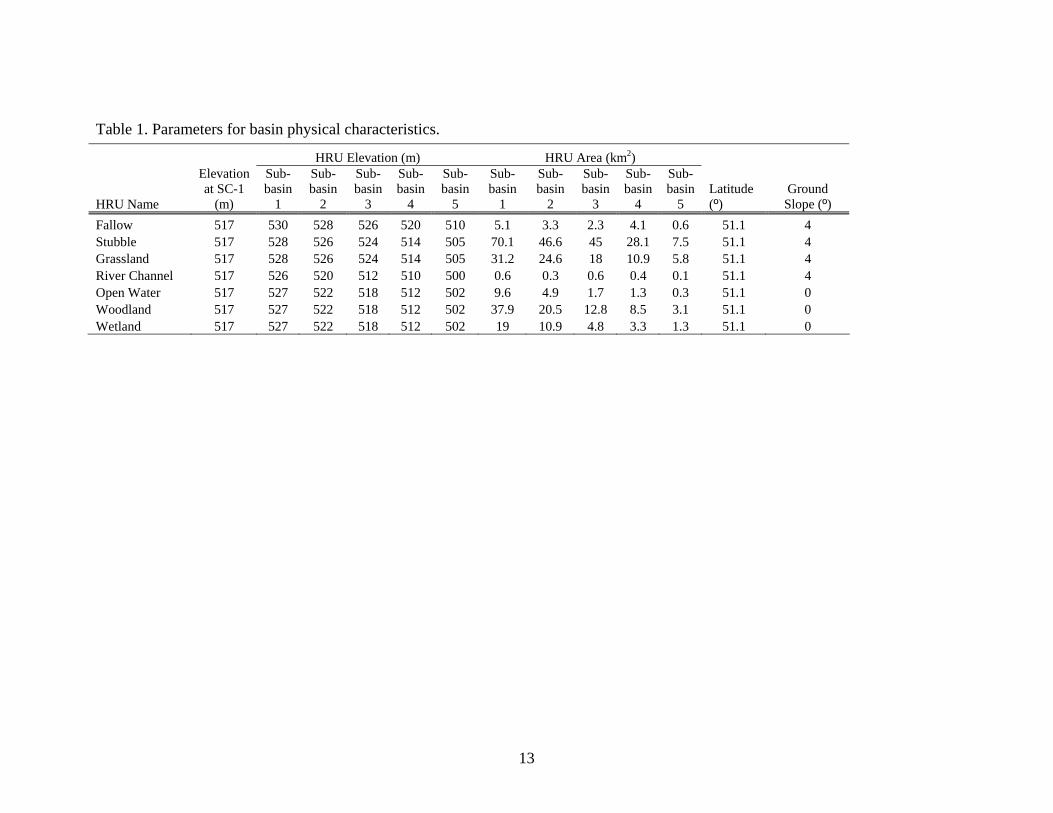
3.3 Model parameters A number of parameters for basin physical characteristics were set up for the seven HRUs, including elevation of meteorological station, HRU elevation, HRU area, latitude, and ground slope. These parameters are essential to the observation, sunshine and radiation modules. The average values of these parameters are shown in Table 1. The elevation at station SC-1 and average elevation for HRU at different sub-basins were determined from a DEM acquired from the DUC GIS dataset. Areas for fallow, stubble, grassland, open water, woodland, and wetland HRUs were decided based on SPOT 5 classification; areas for river channel HRU was determined from DUC drainage GIS dataset. The latitude is the geographic centre of Smith Creek basin and was measured from GPS. The average ground slope was determined from the reported slope values in Saskatchewan Soil Survey (1991). In addition, a list of albedo parameters for bare ground and snow, as well as the canopy parameter LAI (leaf area index), was developed for the HRUs. The values of these parameters are shown in Table 2. The albedo parameters are required in the albedo, evaporation and snowmelt modules; 0.17 and 0.85 were determined for bare ground and snow respectively, based on recommended values by Male and Gray (1981). The canopy parameter, LAI, was used to adjust the radiation module for canopy effects. Small values of LAI (0.001) were set for fallow, stubble, grassland, river channel, open water and wetland HRUs, due to lack of canopy cover above the ground; 0.4 was assigned to woodland HRUs, representing s typical LAI value for aspen trees during the winter at Smith Creek. A set of parameters was also developed for the blowing snow module (Table 3). Blowing snow fetch distance is the upwind distance without disruption to the flow of snow. A computer program “FetchR” (Lapen and Martz, 1993) was used to estimate the fetch for the large exposed areas such as fallow, stubble and grassland HRUs from the DEM and vegetation classification, resulting in 1000 m, 1000 m, and 500 m respectively. For river channel, open water, woodland and wetland HRUs, 300 m was assigned. The vegetation height, stalk density and stalk diameter were calculated based on vegetation survey measurements. The distribution factor parameterizes the allocation of blowing snow transport from aerodynamically smoother (or windier) HRU to aerodynamically rougher (or calmer) ones. Lower values indicate lower aerodynamic roughness (or higher wind

HRU Elevation (m) HRU Area (km2)

HRU Name

Elevation at SC-1

(m)

Sub-basin

1

Sub-basin

2

Sub-basin

3

Sub-basin

4

Sub-basin

5

Sub-basin

1

Sub-basin

2

Sub-basin

3

Sub-basin

4

Sub-basin

5 Latitude (º)

Ground Slope (º)

Fallow 517 530 528 526 520 510 5.1 3.3 2.3 4.1 0.6 51.1 4 Stubble 517 528 526 524 514 505 70.1 46.6 45 28.1 7.5 51.1 4 Grassland 517 528 526 524 514 505 31.2 24.6 18 10.9 5.8 51.1 4 River Channel 517 526 520 512 510 500 0.6 0.3 0.6 0.4 0.1 51.1 4 Open Water 517 527 522 518 512 502 9.6 4.9 1.7 1.3 0.3 51.1 0 Woodland 517 527 522 518 512 502 37.9 20.5 12.8 8.5 3.1 51.1 0 Wetland 517 527 522 518 512 502 19 10.9 4.8 3.3 1.3 51.1 0

13

Table 1. Parameters for basin physical characteristics.

Table 2. Albedo and canopy parameters.

HRU Name Bare Ground Albedo Snow Albedo LAI Fallow 0.17 0.85 0.001 Stubble 0.17 0.85 0.001 Grassland 0.17 0.85 0.001 River Channel 0.17 0.85 0.001 Open Water 0.17 0.85 0.001 Woodland 0.17 0.85 0.4 Wetland 0.17 0.85 0.001

Table 3. Blowing snow parameters.

HRU Name Fetch (m)

Vegetation Height (m)

Stalk Density (#/m2)

Stalk Diameter (m)

Distribution Factor

Fallow 1000 0.001 320 0.003 0.1 Stubble 1000 0.12 320 0.003 0.5 Grassland 500 0.4 320 0.003 1 River Channel 300 0.7 1 0 5 Open Water 300 0.001 1 0 0.5 Woodland 300 6 100 0.01 1 Wetland 300 1.5 100 0.01 10

speed) and higher value means greater roughness (or lower wind speed). Thus, the values presented in Table 3 allow snow to be transported from fallow open water HRUs to stubble HRU and then to grassland according to what was observed in the field. and woodland HRUs, and subsequently to river channel and wetland HRUs. A frozen soil infiltration parameter was set up for HRUs (Table 4). The initial fall soil saturation is important for estimating snowmelt infiltration into frozen soils and was determined from the soil porosity and observed fall soil moisture. The soil porosity was estimated from soil texture, which is predominately loam and clay in Smith Creek. Fall soil moisture was estimated from gravimetric measurement of soil survey samples. Values of 100% for river channel and open water HRUs indicate that both are saturated. Table 4. Frozen soil infiltration parameter.

HRU Name Initial Fall Soil Saturation (%) Fallow 46 Stubble 50 Grassland 54 River Channel 100 Open Water 100 Woodland 53 Wetland 87

A list of key parameters for the new wetland module is present in Table 5. For the soil column, the maximum water holding capacity was determined by multiplying the rooting

14

15

zone depth by soil porosity; the initial value of available water in the soil column was estimated by multiplying the maximum water holding capacity by volumetric soil moisture content. The soil recharge layer is the shallow top layer of the soil column, approximately 60 mm; the initial value of available water in the soil recharge layer was determined by multiplying the maximum water holding capacity and volumetric soil moisture content. It should be noted that the model treats river channel, open water, and wetland HRUs as having no soil column, and sustaining permanent surface ponding. Their maximum storage capacity was determined from a surface area-volume relationship for prairie wetlands derived from the upper Assiniboine Rive basin in eastern Saskatchewan (Wiens, 2001). Small values of initial storage were assigned to small depressions. Subsurface and groundwater drainage factors control the rate of flow in the subsurface and groundwater domains; these rates are slow in the prairie environment (Pomeroy et al., 2007b) and were estimated from the saturated hydraulic conductivity based on soil texture. Parameters for routing surface runoff between HRUs within the sub-basins are shown in Table 6. These parameters were used in the Muskingum routing module (Chow, 1964). The routing length from each HRU to the main channel stream was estimated from DUC stream network GIS dataset. Manning’s equation (Chow, 1959) was used to calculate the average flow velocity; the parameters used in the equation include Manning’s roughness coefficient, hydraulic radius, and longitudinal friction slope. Hydraulic radius was determined from flow depth based on the channel shape. Longitudinal friction slope was calculated from the DEM and DUC stream network GIS dataset; the average change in HRU elevation over a certain length to the stream was approximated. Manning’s roughness coefficient was estimated based on the channel’s condition. From the average flow velocity and routing length, the storage constant was estimated. The dimensionless weighting factor controls the level of attenuation, ranging from 0 (maximum attenuation) to 0.5 (no attenuation); 0.25 was used for Smith Creek. The routing order determines the direction of surface runoff; the routing destination specifies where the runoff from one HRU goes to, 0 indicating directly to the basin outlet and other numbers indicating the destination HRU number. A set of parameters for routing channel flow between RBs was set up for the five sub-basins (Table 7). The Muskingum routing method (Chow, 1964) was used for routing flow in the channel. The routing length is the main channel length in each sub-basin and was estimated from DUC stream network GIS dataset. Hydraulic radius is the function of a cross-sectional area of flow in the channel and the wetted perimeter of flow; it was determined from the flow depth based on channel shape. Longitudinal friction slope was calculated from the DUC stream network GIS dataset; the average change in elevation over a certain length of stream was approximated from the GIS. Manning’s roughness coefficient was estimated based on the channel condition based on visual inspection. All these parameters were used in Manning’s equation (Chow, 1959) to calculate the average flow velocity. Based on the average flow velocity and routing length, the storage constant parameter, or travel time of flow in the channel, was calculated. The dimensionless weighting factor controls the attenuation level, ranging from 0 (maximum attenuation) to 0.5 (no attenuation); 0.25 was used for Smith Creek. The routing order parameter

16

Table 5. Wetland module parameters.

Table 6. Parameters of Muskingum routing between HRUs within sub-basin.

Routing Length to Stream (m)

HRU Name

Sub-basin

1

Sub-basin

2

Sub-basin

3

Sub-basin

4

Sub-basin

5

Manning's Roughness Coefficient

Hydraulic Radius

(m)

Longitudinal Friction Slope

(º)

Dimensionless Weighting

Factor Routing Order

Routing Destination

Fallow 6000 5000 5000 4000 2000 0.04 0.01 0.001 0.25 1 7 Stubble 6000 5000 5000 4000 2000 0.05 0.01 0.001 0.25 2 7 Grassland 6000 5000 5000 4000 2000 0.11 0.01 0.001 0.25 3 7 River Channel 6000 5000 5000 4000 2000 0.035 0.01 0.001 0.25 6 0 Open Water 6000 5000 5000 4000 2000 0.11 0.01 0.00002 0.25 7 4 Woodland 6000 5000 5000 4000 2000 0.2 0.01 0.00002 0.25 5 7 Wetland 6000 5000 5000 4000 2000 0.2 0.01 0.00002 0.25 4 5

Soil Recharge Layer Soil Column Surface Depression Storage

HRU Name

Initial Value of Available Water (mm)

Maximum Water Holding

Capacity (mm)

Initial Value of Available Water (mm)

Maximum Water Holding Capacity (mm)

Initial Value (mm)

Maximum Storage Capacity

(mm) Subsurface and Groundwater

Drainage Factor (mm/day) Fallow 28 60 276 600 0 5 0.001 Stubble 30 60 300 600 0 5 0.001 Grassland 32 60 324 600 0 5 0.001 River Channel 0 0 0 0 40 200 0.001 Open Water 0 0 0 0 45 420 0.001 Woodland 32 60 318 600 0 0 0.001 Wetland 0 0 0 0 45 420 0.001

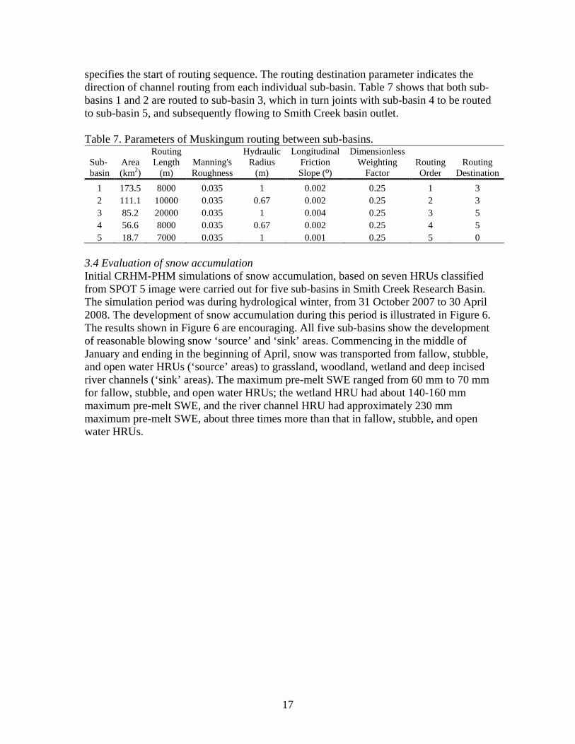
specifies the start of routing sequence. The routing destination parameter indicates the direction of channel routing from each individual sub-basin. Table 7 shows that both sub-basins 1 and 2 are routed to sub-basin 3, which in turn joints with sub-basin 4 to be routed to sub-basin 5, and subsequently flowing to Smith Creek basin outlet. Table 7. Parameters of Muskingum routing between sub-basins.

Sub-basin

Area (km2)

Routing Length

(m) Manning's Roughness

Hydraulic Radius

(m)

Longitudinal Friction Slope (º)

Dimensionless Weighting

Factor Routing Order

Routing Destination

1 173.5 8000 0.035 1 0.002 0.25 1 3 2 111.1 10000 0.035 0.67 0.002 0.25 2 3 3 85.2 20000 0.035 1 0.004 0.25 3 5 4 56.6 8000 0.035 0.67 0.002 0.25 4 5 5 18.7 7000 0.035 1 0.001 0.25 5 0

3.4 Evaluation of snow accumulation Initial CRHM-PHM simulations of snow accumulation, based on seven HRUs classified from SPOT 5 image were carried out for five sub-basins in Smith Creek Research Basin. The simulation period was during hydrological winter, from 31 October 2007 to 30 April 2008. The development of snow accumulation during this period is illustrated in Figure 6. The results shown in Figure 6 are encouraging. All five sub-basins show the development of reasonable blowing snow ‘source’ and ‘sink’ areas. Commencing in the middle of January and ending in the beginning of April, snow was transported from fallow, stubble, and open water HRUs (‘source’ areas) to grassland, woodland, wetland and deep incised river channels (‘sink’ areas). The maximum pre-melt SWE ranged from 60 mm to 70 mm for fallow, stubble, and open water HRUs; the wetland HRU had about 140-160 mm maximum pre-melt SWE, and the river channel HRU had approximately 230 mm maximum pre-melt SWE, about three times more than that in fallow, stubble, and open water HRUs.

17

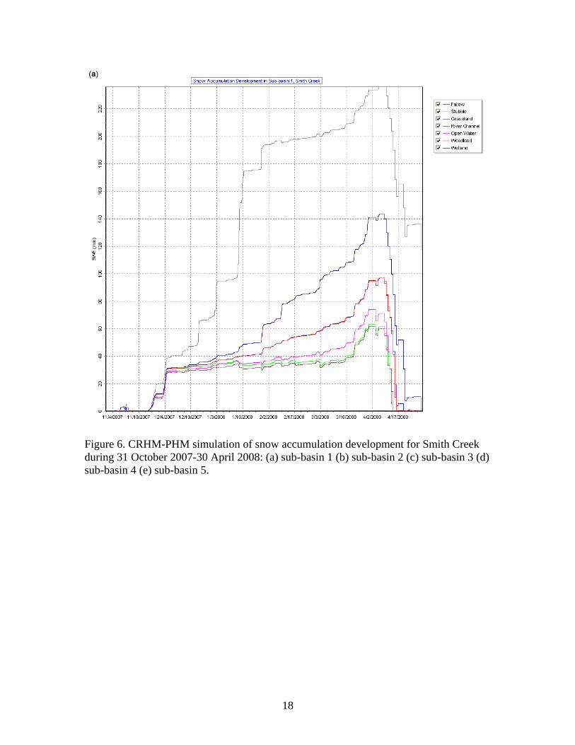
Figure 6. CRHM-PHM simulation of snow accumulation development for Smith Creek during 31 October 2007-30 April 2008: (a) sub-basin 1 (b) sub-basin 2 (c) sub-basin 3 (d) sub-basin 4 (e) sub-basin 5.

18

Figure 6. Continued.

19

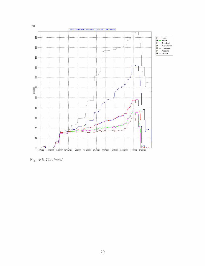
Figure 6. Continued.

20

Figure 6. Continued.

21

Figure 6. Concluded.

22

In addition, the simulated snow accumulation was compared to the observed accumulation for seven HRUs in each sub-basin during both pre-melt and melt periods. During the pre-melt period, three surveys of SWE were conducted - on the 7th and 28th of February, and on the 20th of March. During the melt period, four surveys of SWE were carried out during 11- 14 April. Figure 7 shows the comparison of these observed SWE and corresponding simulations for fallow, stubble, grassland, river channel, open water, woodland and wetland HRUs in sub-basin 1. There is generally good agreement between the observed SWE and simulated SWE for most HRUs; however, a relatively large difference between the observation and simulation exists for fallow, stubble, grassland and open water HRUs during the melt period. This may be related to the uncertainty of determining HRUs area from SPOT 5 image classification or to cumulative errors in the snowmelt routine. The comparison between the observed SWE and simulated SWE for the seven HRUs show very similar results for other four sub-basins and are not shown in this report.

Snow Accumulation in Fallow Field from Smith Creek Sub-basin 1

0

5

10

15

20

25

30

35

40

45

02-Feb-08 12-Feb-08 22-Feb-08 03-Mar-08 13-Mar-08 23-Mar-08 02-Apr-08 12-Apr-08 22-Apr-08

SW

E (m

m)

ObservedSimulated

(a)

Figure 7. Comparison of simulated and observed snow accumulation during pre-melt and melt periods for seven HRUs at sub-basin 1, Smith Creek (a) fallow (b) stubble (c) grassland (d) river channel (e) open water (f) woodland (g) wetland.

23

Snow Accumulation in Stubble Field from Smith Creek Sub-basin 1

0

5

10

15

20

25

30

35

40

45

50

02-Feb-08

12-Feb-08

22-Feb-08

03-Mar-08

13-Mar-08

23-Mar-08

02-Apr-08

12-Apr-08

22-Apr-08

SWE

(mm

)

ObservedSimulated

(b)

Snow Accumulation in Grassland from Smith Creek Sub-basin 1

0

10

20

30

40

50

60

70

80

02-Feb-08

12-Feb-08

22-Feb-08

03-Mar-08

13-Mar-08

23-Mar-08

02-Apr-08

12-Apr-08

22-Apr-08

SWE

(mm

)

ObservedSimulated

(c)

Figure 7. Continued.

24

Snow Accumulation in River Channel from Smith Creek Sub-basin 1

0

50

100

150

200

250

300

02-Feb-08

12-Feb-08

22-Feb-08

03-Mar-08

13-Mar-08

23-Mar-08

02-Apr-08

12-Apr-08

22-Apr-08

SWE

(mm

)

ObservedSimulated

(d)

Snow Accumulation in Open Water from Smith Creek Sub-basin 1

0

10

20

30

40

50

60

02-Feb-08

12-Feb-08

22-Feb-08

03-Mar-08

13-Mar-08

23-Mar-08

02-Apr-08

12-Apr-08

22-Apr-08

SWE

(mm

)

ObservedSimulated

(e)

Figure 7. Continued.

25

Snow Accumulation in Woodland from Smith Creek Sub-basin 1

0

10

20

30

40

50

60

70

80

90

02-Feb-08

12-Feb-08

22-Feb-08

03-Mar-08

13-Mar-08

23-Mar-08

02-Apr-08

12-Apr-08

22-Apr-08

SWE

(mm

)

ObservedSimulated

(f)

Snow Accumulation in Wetland from Smith Creek Sub-basin 1

0

20

40

60

80

100

120

140

02-Feb-08

12-Feb-08

22-Feb-08

03-Mar-08

13-Mar-08

23-Mar-08

02-Apr-08

12-Apr-08

22-Apr-08

SWE

(mm

)

ObservedSimulated

(g)

Figure 7. Concluded.

26

To quantify the difference between the observed and simulated SWE, the Root Mean Square Difference (RMSD) was calculated for the seven HRUs (Table 8). The RMSD is a weighted measure of the difference between observed and predicted SWE and has the same units as the observed and predicted SWE. For all five sub-basins, the RMSD was relatively small for fallow, stubble, open water and woodland HRUs, the values ranging from 1.8 mm to 7.9 mm. The Wetland HRU had moderately large values of RMSD, between 6.7 mm and 13.7 mm. Values of RMSD were similar for grassland and river channel HRUs, ranging from 11.6 mm to 17.5 mm. However, these larger values of RMSD for wetland and river channel are still within the acceptable level, considering their peak pre-melt SWE ranges from 140 mm to 230 mm. Table 8. Evaluation of CRHM-PHM performance in snow accumulation simulation with Root Mean Square Difference (mm SWE).

HRU Name Sub-basin 1 Sub-basin 2 Sub-basin 3 Sub-basin 4 Sub-basin 5 Fallow 2.7 1.8 2.7 2.6 1.8 Stubble 3.4 3.3 7.0 6.8 6.1 Grassland 14.4 12.7 12.7 13.4 13.1 River Channel 17.5 17.5 11.6 12.6 12.2 Open Water 5.5 5.5 5.5 5.5 7.9 Woodland 2.7 2.7 2.7 2.7 2.7 Wetland 6.7 8.3 12.7 13.7 6.4

3.5 Evaluation of runoff and streamflow discharge The surface runoff between HRUs in the sub-basins and channel flow between sub-basins were routed using the Muskingum routing method. At the outlet of the five sub-basins, with no calibration, the springtime discharge was simulated during the runoff period (10-30 April 2008), and the hourly instantaneous discharge is shown in Figure 8. Discharges at sub-basin 1, 2, and 4 were also measured on five days, 16-17 and 21-23 April. The measured discharges were only instantaneous values between 1400 and 1500 hours and it must be noted that this is therefore a very limited model test. The comparison of measured discharges and corresponding simulated discharges is presented in Figure 9. For the sub-basin 1 outlet, there was no discharge simulated by the model during these five discharge observation days, but rather the simulated discharge started appearing on 25 April, about two days delayed. There are large numbers of depressions, ponds, and lakes in the sub-basin 1, the depression/pond storage capacity and routing parameters set up in the model contributed to this delay. The simulated discharge was somewhat comparable to the observed discharge at the sub-basin 1 outlet; while the difference between simulated and observed discharges was quite large for both sub-basin 2 and 4. However, the magnitude of these observed instantaneous discharges is very small, ranging from 0.03 to 1.2 m3/s. For a simulation without calibration, the model is unable to accurately estimate such small magnitudes of discharge. The model performance in simulating streamflow discharge was evaluated in the hydrological years of 1994-95 and 2001-02. These are two distinct years: with a large runoff event in spring of 1995, and a drought in the spring of 2002. The purpose is to find out how the model’s performance is different under extremely wet and dry conditions.

27

Springtime Hourly Discharge of Smith Creek Sub-basins

0

2

4

6

8

10

12

14

10/0

4/20

08

11/0

4/20

08

12/0

4/20

08

13/0

4/20

08

14/0

4/20

08

15/0

4/20

08

16/0

4/20

08

17/0

4/20

08

18/0

4/20

08

19/0

4/20

08

20/0

4/20

08

21/0

4/20

08

22/0

4/20

08

23/0

4/20

08

24/0

4/20

08

25/0

4/20

08

26/0

4/20

08

27/0

4/20

08

28/0

4/20

08

29/0

4/20

08

30/0

4/20

08

01/0

5/20

08

Inst

anta

neou

s Di

scha

rge

(m3 /s

) Sub-basin 1Sub-basin 2Sub-basin 3Sub-basin 4Sub-basin 5

Figure 8. Hourly instantaneous discharge at sub-basins of Smith Creek during spring runoff period, 2008.

Springtime Dicharge of Smith Creek Sub-basin 1

0

0.2

0.4

0.6

0.8

1

1.2

1.4

16/04

/2008

17/04

/2008

18/04

/2008

19/04

/2008

20/04

/2008

21/04

/2008

22/04

/2008

23/04

/2008

24/04

/2008

25/04

/2008

26/04

/2008

27/04

/2008

28/04

/2008

Inst

anta

neou

s D

isch

arge

(m3 /s

) ObservedSimulated

(a)

Figure 9. Comparison of observed and simulated springtime hourly instantaneous discharge at sub-basins of Smith Creek (a) sub-basin 1 (b) sub-basin 2 (c) sub-basin 4.

28

Springtime Dicharge of Smith Creek Sub-basin 2

0

0.5

1

1.5

2

2.5

3

3.5

16/04

/2008

17/04

/2008

18/04

/2008

19/04

/2008

20/04

/2008

21/04

/2008

22/04

/2008

23/04

/2008

Inst

anta

neou

s D

isch

arge

(m3 /s

) ObservedSimulated

(b)

Springtime Dicharge of Smith Creek Sub-basin 4

0

1

2

3

4

5

6

16/04

/2008

17/04

/2008

18/04

/2008

19/04

/2008

20/04

/2008

21/04

/2008

22/04

/2008

23/04

/2008

Inst

anta

neou

s D

isch

arge

(m3 /s

) ObservedSimulated

(c)

Figure 9. Concluded.

29

The meteorological data for these two years was obtained from Environment Canada Weather Office historical database for Langenburg and Yorkton. The precipitation adjustment between Langenburg and Yorkton was conducted based on the Double Mass Curve method; the purpose is to replace the missing precipitation data in Langenburg with the adjusted precipitation from Yorkton. The incident short-wave radiation was estimated from sunshine hour data acquired from Environment Canada meteorology database. Initial conditions of soil moisture content were derived from soil moisture dataset supplied by Manitoba Water Stewardship. DUC historical (1958) upland landcover inventory was adjusted by the changes in individual landcover between 1958 and 1994 and between 1958 and 2001; the landcover information for 1994 and 2001 was derived from Census of Agriculture in Churchbridge and Langenburg. The adjusted DUC upland landcover was used for 1994 and 2001. Based on the same modelling structure, the daily streamflow discharge of Smith Creek near Marchwell was simulated and compared to the observed streamflow discharge (Figure 10). In the spring of 1995, simulated and observed peak daily discharges are comparable, 24.6 and 22.6 m3/s, respectively. The timing of the simulated peak discharge is late; the peak daily discharge was observed on 25 April, while the model simulated it on 8 May, about two weeks behind. In the spring of 2002, the peak daily discharges are much smaller, 0.16 and 1.04 m3/s for the simulated and observed, respectively. The predicted peak daily discharge on 11 May is more three weeks behind the observed one on 16 April. To quantify the model’s performance, Root Mean Square Difference (RMSD) and Model Bias (MB) were calculated. RMSD is a weighted measure of the difference between simulated and observed discharges and has the same units as m3/s. MB is dimensionless index for annual water balance, a positive bias indicates overprediction and a negative bias indicates underprediction. Values of RMSD are 0.2 and 0.005 m3/s for the simulated daily discharges in 1994-95 and 2001-02, respectively; both are relatively small to the respective peak daily discharges. However, -0.13 and -0.93 are values of MB for the simulated daily discharges in 1994-95 and 2001-02, respectively. This indicates that the total annual discharge predicted by the model is 13% and 93% less than the observation for hydrological years of 1994-95 and 2001-02, respectively. Even though the model’s simulated peak daily discharge is behind by two to three weeks, the averaged errors of simulated daily discharge are quite small for both wet and dry years. For the total annual discharge, the model has better performance in a wet year than in a dry year. It is assumed that these errors could be reduced by calibration of parameters or by inclusion of a more accurate DEM as derived from LiDAR data. 4. Characterization of wetland storage Within the Smith Creek Research Basin, 14 wetlands were selected for a detailed topographic survey. These data were used to create a high resolution digital elevation model (DEM) which allowed for accurate volume measurements of each wetland. These volume calculations were compared to the estimated volume produced by three different methods. The Volume-Area-Depth (V-A-D) relationship developed by Hayashi and van der Kamp (2000) was found to estimate volume and area particularly well for all wetlands. The errors associated with this method were <5% for volume and <10% for

30

Discharge of Smith Creek near Marchwell

0

5

10

15

20

25

30

31/1

0/19

94

30/1

1/19

94

31/1

2/19

94

31/0

1/19

95

28/0

2/19

95

31/0

3/19

95

30/0

4/19

95

31/0

5/19

95

30/0

6/19

95

31/0

7/19

95

31/0

8/19

95

30/0

9/19

95

Daily

Mea

n Di

scha

rge

(m3 /s

) ObservedSimulated

MB = -0.13 RMSD = 0.2

Discharge of Smith Creek near Marchwell

0

0.2

0.4

0.6

0.8

1

1.2

31/1

0/20

01

30/1

1/20

01

31/1

2/20

01

31/0

1/20

02

28/0

2/20

02

31/0

3/20

02

30/0

4/20

02

31/0

5/20

02

30/0

6/20

02

31/0

7/20

02

31/0

8/20

02

30/0

9/20

02

Daily

Mea

n D

isch

arge

(m3 /s

) ObservedSimulated

MB = -0.93 RMSD = 0.005

Figure 10. Comparison of observed and simulated daily discharge of Smith Creek near Marchwell for hydrological years of 1994-95 and 2001-02.

31

area. This level of error is within the limit that Hayashi and van der Kamp (2000) advocate as acceptable. The Volume-Area regression method used in the Upper Assiniboine River Basin Study (Wiens, 2001) was tested on eight wetlands in Smith Creek. The surface area measurements were extracted from DUC wetland GIS dataset and were used as input to the regression formula. This method ranged from underestimating volume by 46% to overestimating volume by 30% (Figure 11). These results indicate that the Volume-Area regression method used in the Upper Assiniboine River Basin Study has limitations for accurately estimating wetland storage. The last method tested was a simplified version of the Hayashi and van der Kamp V-A-D relationship. This method is advantageous because it does not require a topographic survey yet it still incorporates information on the wetland depression. The required inputs for this method are two measurements of wetland surface area and depth. These measurements should have sufficient time between them that the natural fluctuations in water storage are reflected by the measurements. The simplified V-A-D relationship was found to estimate volume and area well, with errors of <10%.

Figure 11. Comparison of wetland volume calculation methods. There is a potential to apply the simplified V-A-D method to all wetlands in Smith Creek if adequate quality topographic information is available. This would involve utilizing remote sensing and a high resolution LiDAR DEM of the entire basin to provide the surface area and bathymetry of dry wetlands. These data will enable the Hayashi and van der Kamp coefficients to be calculated and the simplified method to be applied. Given the

32

performance of the Upper Assiniboine River Basin method, it should be possible to make improvements to storage estimations if the simplified Hayashi and van der Kamp (2000) V-A-D relationship can be applied. 5. Conclusions A new wetland module was successfully incorporated into the CRHM-PHM, which completed the model structure and requirement for simulating prairie hydrological processes and water balance. Smith Creek was broken down into five sub-basins and seven landcover based HRUs were set up for each sub-basin. Various datasets (DUC drainage network, wetland inventory, topographic map based DEM) and information derived from field surveys of soil properties and vegetation were used for determining values of model parameters. Simulations of CRHM-PHM were conducted and model performances in predicting snow accumulations and streamflow discharge were evaluated. The model had generally good performance in predicted snow accumulation in pre-melt and melt periods for most of HRUs, and better simulation for streamflow discharge was found for a wet year than for a dry year. Topographic surveys were carried out to characterize wetland storage volumes. Various methods: Hayashi and van der Kamp V-A-D relationship, the Upper Assiniboine River Basin V-A regression method, and simplified Hayashi and van der Kamp V-A-D relationship were used to calculate the wetland volume. The calculated volume and measured volumes were compared. Both the Hayashi and van der Kamp V-A-D relationship and its simplified version had results very comparable to the measured values and higher accuracy than the Upper Assiniboine River Basin V-A regression method. The simplified Hayashi and van der Kamp V-A-D relationship can be applied for estimating wetland storage for entire Smith Creek provided that high resolution of LiDAR DEM is available.

33

References Chow, V.T. 1959. Open Channel Hydraulics. McGraw-Hill, Inc. New York, USA. Chow, V.T. 1964. Handbook of Applied Hydrology. McGraw-Hill, Inc. New York, USA. Dornes, P.F., Pomeroy, J.W., Pietroniro, A., Carey, S.K. and Quinton, W. L. 2008.

Influence of landscape aggregation in modelling snow-cover ablation and snowmelt runoff in a sub-arctic mountainous environment. Hydrological Sciences Journal, 53(4), 725-740.

Fang, X. and Pomeroy, J.W. 2007. Snowmelt runoff sensitivity analysis to drought on the Canadian Prairies. Hydrological Processes 21: 2594-2609.

Fang, X. and Pomeroy, J.W. 2008. Drought impacts on Canadian prairie wetland snow hydrology. Hydrological Processes 22: 2858-2873.

Garnier, B.J. and Ohmura, A. 1970. The evaluation of surface variations in solar radiation income. Solar Energy 13: 21-34.

Granger, R.J. and Gray, D.M. 1989. Evaporation from natural non-saturated surfaces. Journal of Hydrology 111: 21–29.

Gray, D.M., Landine, P.G. and Granger, R.J. 1985. Simulating infiltration into frozen Prairie soils in stream flow models. Canadian Journal of Earth Science 22: 464-474.

Gray, D.M. and Landine, P.G. 1987. Albedo model for shallow prairie snow covers. Canadian Journal of Earth Sciences 24: 1760-1768.

Gray, D.M. and Landine, P.G. 1988. An energy-budget snowmelt model for the Canadian Prairies. Canadian Journal of Earth Sciences 25: 1292-1303.

Hayashi, M. and van der Kamp, G. 2000. Simple equations to represent the volume-area-depth relations of shallow wetlands in small topographic depressions. Journal of Hydrology 237: 74-85.

Lapen, D.R. and Martz, L.W. 1993. The measurement of two simple topographic indices of wind sheltering exposure from raster digital elevation models. Computer & Geosciences 19: 769-779.

Leavesley, G.H., Lichty, R.W., Troutman, B.M. and Saindon, L.G. 1983. Precipitation-runoff modelling system: user’s manual. US Geological Survey Water Resources Investigations Report 83-4238. 207 pp.

Male, D.H. and Gray, D.M. 1981. Snowcover ablation and runoff. In Gray, D.M. and Male, D.H. (Eds.), Handbook of Snow: principles, processes, management & use. Ontario: Pergamon Press Canada Ltd., pp. 360-436.

Ogden, F.L. and Saghafian, B. 1997. Green and Ampt infiltration with redistribution. Journal of Irrigation and Drainage Engineering 123: 386-393.

Pomeroy, J.W. and Li, L. 2000. Prairie and Arctic areal snow cover mass balance using a blowing snow model. Journal of Geophysical Research 105: 26619-26634.

Pomeroy, J.W., Gray, D.M., Brown, T., Hedstrom, N.R., Quinton, W., Granger, R.J. and Carey, S. 2007a. The Cold Regions Hydrological Model, a platform for basing process representation and model structure on physical evidence. Hydrological Processes 21: 2650-2667.

Pomeroy, J.W., de Boer, D. and L. Martz. 2007b. Hydrology and water resources. In, (eds. B. Thraves, M. Lewry, J Dale, H. Schlichtmann) Saskatchewan: Geographic Perspectives. Canadian Plains Research Centre, Regina, SK. 63-80.

34

Pomeroy, J.W., Westbrook, C., Fang, X., Minke, A. and Guo, X. 2008. Prairie Hydrological Model Study Progress Report, April 2008. Centre for Hydrology Report No.3, University of Saskatchewan, p.18

Priestley, C.H.B. and Taylor, R.J. 1972. On the assessment of surface heat flux and evaporation using large-scale parameters. Monthly Weather Review 100: 81-92.

Saskatchewan Soil Survey. 1991. The soils of Langenburg (181), Fertile Belt (183), Churchbridge (211), Saltcoats (213) rural municipalities Saskatchewan. Saskatchewan Institute of Pedology, Publication S208, Saskatoon, p.79.

Sicart, J.E., Pomeroy, J.W., Essery, R.L.H., Hardy, J., Link, T. and Marks, D. 2004. A sensitivity study of daytime net radiation during snowmelt to forest canopy and atmospheric conditions. Journal of Hydrometeorology 5: 774-784.

Spence, C., and J. Hosler, 2007. Representation of stores along drainage networks in heterogeneous landscapes for runoff modelling. Journal of Hydrology 347: 474-486.

Walmsley, J.L., Taylor, P.A. and Salmon, J.R. 1989. Simple guidelines for estimating windspeed variations due to small-scale topographic features – an update. Climatological Bulletin 23: 3-14.

Wiens, L.H. 2001. A surface area-volume relationship for prairie wetlands in the upper Assiniboine River basin, Saskatchewan. Canadian Water Resources Journal 26: 503-513.

35