Practical Lessons using Propensity Scores to Generate Comparison Groups for Persistence Research

Jennifer Lowman, Ph.D.

Coordinator, Student Persistence Research

University of Nevada, Reno

Outline

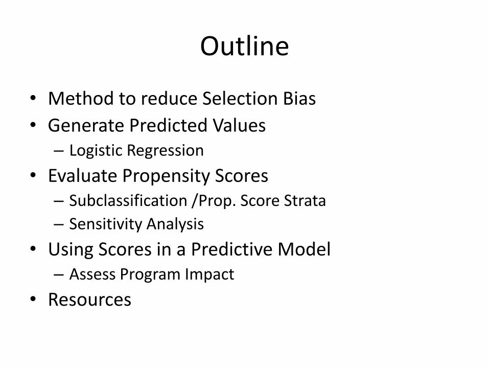
• Method to reduce Selection Bias

• Generate Predicted Values – Logistic Regression

• Evaluate Propensity Scores – Subclassification /Prop. Score Strata

– Sensitivity Analysis

• Using Scores in a Predictive Model – Assess Program Impact

• Resources

Selection Bias

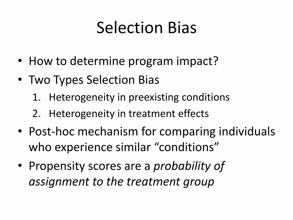
• How to determine program impact?

• Two Types Selection Bias

1. Heterogeneity in preexisting conditions

2. Heterogeneity in treatment effects

• Post-hoc mechanism for comparing individuals who experience similar “conditions”

• Propensity scores are a probability of assignment to the treatment group

Propensity Scores

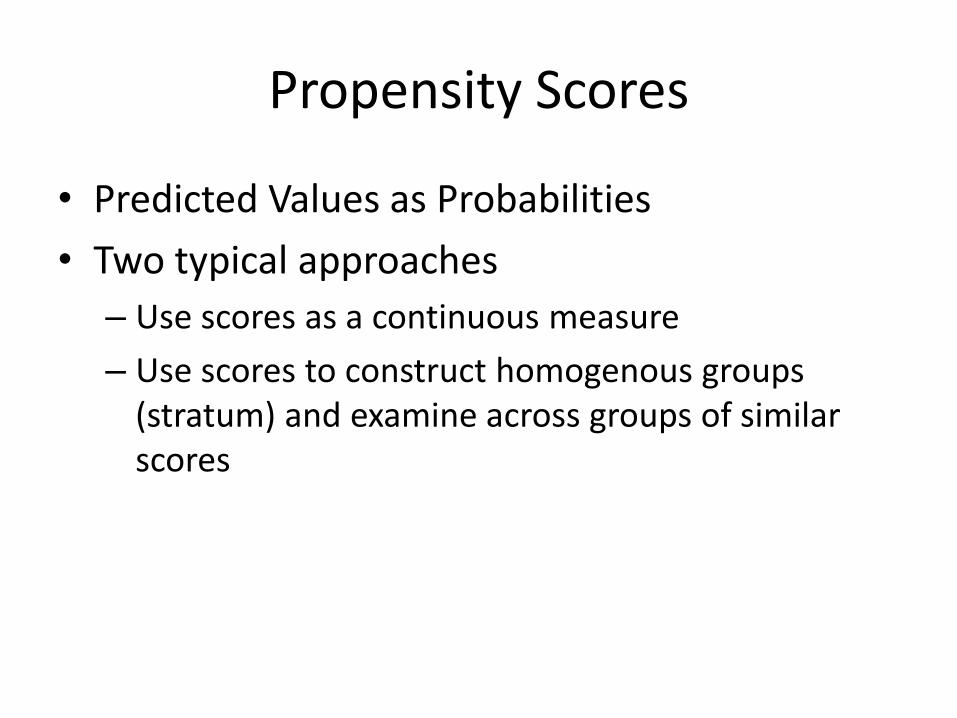
• Predicted Values as Probabilities

• Two typical approaches

– Use scores as a continuous measure

– Use scores to construct homogenous groups (stratum) and examine across groups of similar scores

Generate Predicted Values

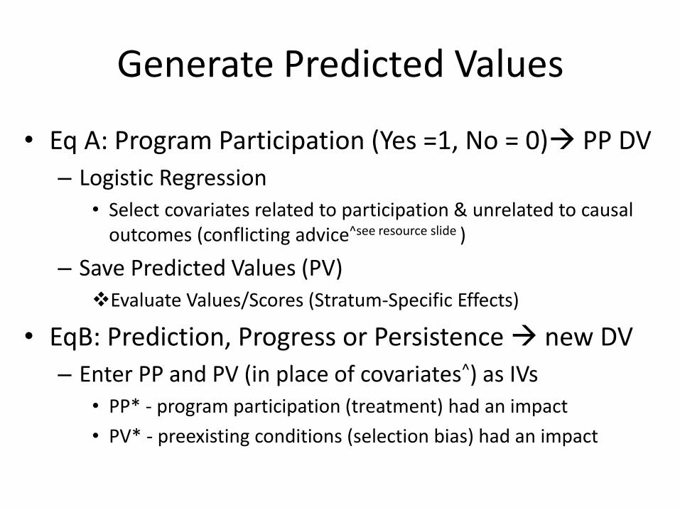
• Eq A: Program Participation (Yes =1, No = 0) PP DV

– Logistic Regression

• Select covariates related to participation & unrelated to causal outcomes (conflicting advice^see resource slide )

– Save Predicted Values (PV)

Evaluate Values/Scores (Stratum-Specific Effects)

• EqB: Prediction, Progress or Persistence new DV

– Enter PP and PV (in place of covariates^) as IVs

• PP* - program participation (treatment) had an impact

• PV* - preexisting conditions (selection bias) had an impact

SPSS

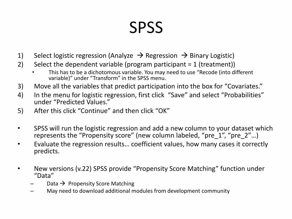
1) Select logistic regression (Analyze Regression Binary Logistic) 2) Select the dependent variable (program participant = 1 (treatment))

• This has to be a dichotomous variable. You may need to use “Recode (into different variable)” under “Transform” in the SPSS menu.

3) Move all the variables that predict participation into the box for “Covariates.” 4) In the menu for logistic regression, first click “Save” and select “Probabilities”

under “Predicted Values.” 5) After this click “Continue” and then click “OK” • SPSS will run the logistic regression and add a new column to your dataset which

represents the “Propensity score” (new column labeled, “pre_1”, “pre_2”…) • Evaluate the regression results… coefficient values, how many cases it correctly

predicts.

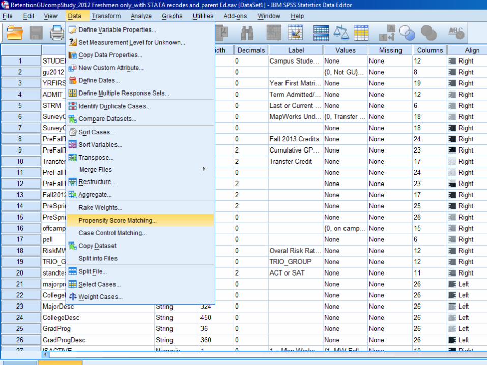
• New versions (v.22) SPSS provide “Propensity Score Matching” function under “Data”

– Data Propensity Score Matching – May need to download additional modules from development community

STATA

• logit or logistic regression commands

(1) logistic DV treatment variable …variable list

(2) predict xb

• Becker & Ichino’s ado file “pscore” – With documentation The STATA Journal

(1) pscore DV [variable list], pscore (new)

…blockid (new variable) detail numblo(#)

details necessary to examine balancing

Evaluating Propensity Scores

• Distribution diagnostics – Examine probabilities for program participation

– Correct or Incorrect Classification

• Subclassification into Strata – 5-Strata^see resources, Cochran 1968 removes 90% bias

– “Balancing” Strata • Minimize differences on mean within each interval

• Matching means on covariates

• Estimate Strata-Specific Effects – sensitivity analysis

Balancing Method

• Within each interval, the average propensity score of treated and control is tested to determine is groups differ

• If the test fails in one interval, splits the interval in half and tests again

• Continue until, in all intervals, the average propensity score of treated and control units does not differ.

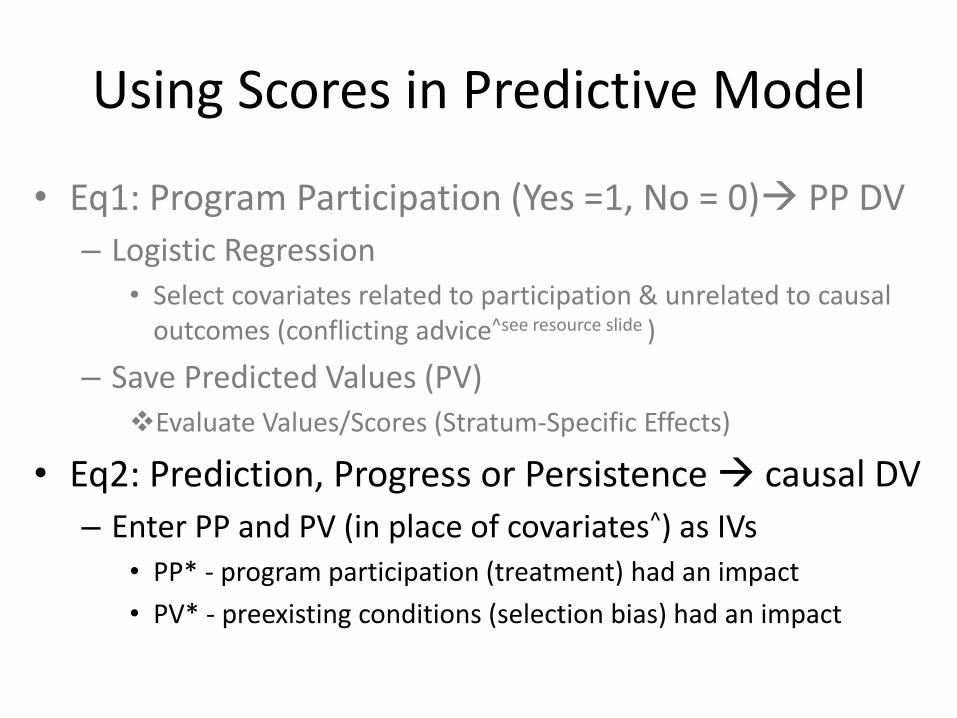
Using Scores in Predictive Model

• Eq1: Program Participation (Yes =1, No = 0) PP DV

– Logistic Regression

• Select covariates related to participation & unrelated to causal outcomes (conflicting advice^see resource slide )

– Save Predicted Values (PV)

Evaluate Values/Scores (Stratum-Specific Effects)

• Eq2: Prediction, Progress or Persistence causal DV

– Enter PP and PV (in place of covariates^) as IVs

• PP* - program participation (treatment) had an impact

• PV* - preexisting conditions (selection bias) had an impact

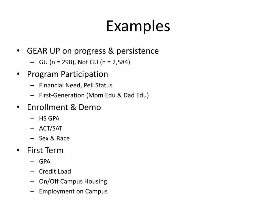
Examples

• GEAR UP on progress & persistence – GU (n = 298), Not GU (n = 2,584)

• Program Participation – Financial Need, Pell Status

– First-Generation (Mom Edu & Dad Edu)

• Enrollment & Demo – HS GPA

– ACT/SAT

– Sex & Race

• First Term – GPA

– Credit Load

– On/Off Campus Housing

– Employment on Campus

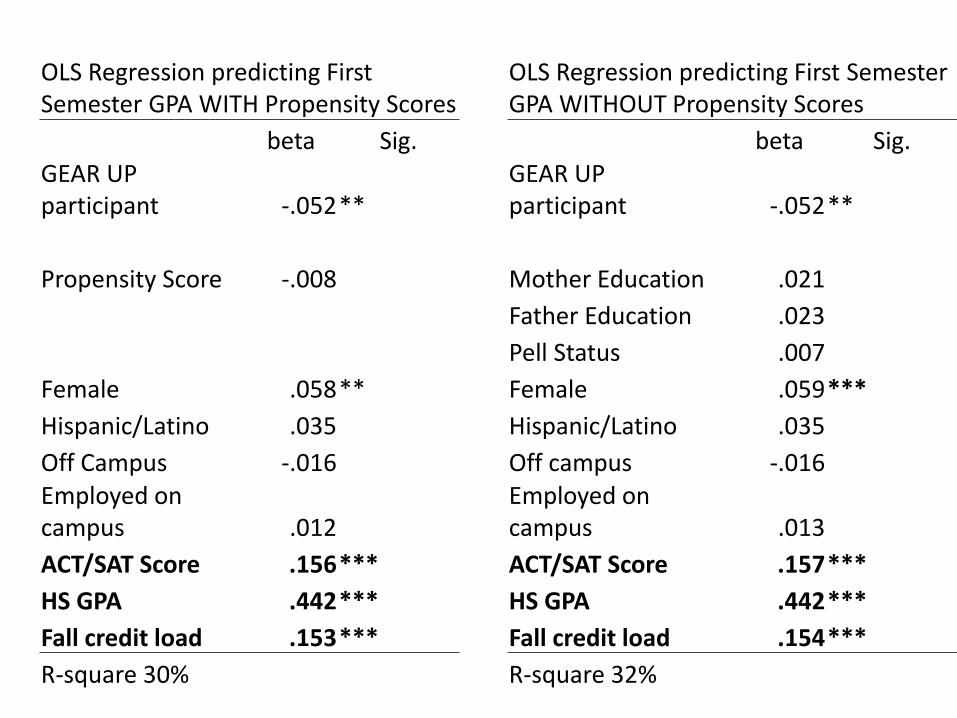
OLS Regression predicting First Semester GPA WITH Propensity Scores

OLS Regression predicting First Semester GPA WITHOUT Propensity Scores

beta Sig. beta Sig. GEAR UP participant -.052 **

GEAR UP participant -.052 **

Propensity Score -.008 Mother Education .021

Father Education .023

Pell Status .007

Female .058 ** Female .059 ***

Hispanic/Latino .035 Hispanic/Latino .035

Off Campus -.016 Off campus -.016 Employed on campus .012

Employed on campus .013

ACT/SAT Score .156 *** ACT/SAT Score .157 ***

HS GPA .442 *** HS GPA .442 ***

Fall credit load .153 *** Fall credit load .154 ***

R-square 30% R-square 32%

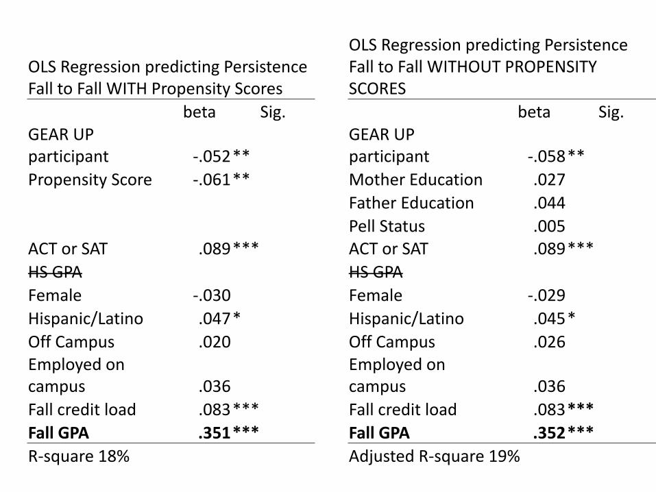
OLS Regression predicting Persistence Fall to Fall WITH Propensity Scores

OLS Regression predicting Persistence Fall to Fall WITHOUT PROPENSITY SCORES

beta Sig. beta Sig. GEAR UP participant -.052 **

GEAR UP participant -.058 **

Propensity Score -.061 ** Mother Education .027

Father Education .044

Pell Status .005 ACT or SAT .089 *** ACT or SAT .089 ***

HS GPA HS GPA

Female -.030 Female -.029

Hispanic/Latino .047 * Hispanic/Latino .045 *

Off Campus .020 Off Campus .026 Employed on campus .036

Employed on campus .036

Fall credit load .083 *** Fall credit load .083 ***

Fall GPA .351 *** Fall GPA .352 ***

R-square 18% Adjusted R-square 19%

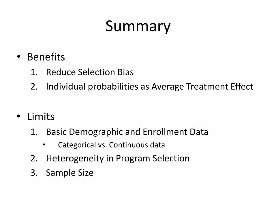
Summary

• Benefits

1. Reduce Selection Bias

2. Individual probabilities as Average Treatment Effect

• Limits

1. Basic Demographic and Enrollment Data

• Categorical vs. Continuous data

2. Heterogeneity in Program Selection

3. Sample Size

Access to Notes

www.unr.edu/ateam/researchmethods

Jennifer Lowman, jlowman@unr.edu

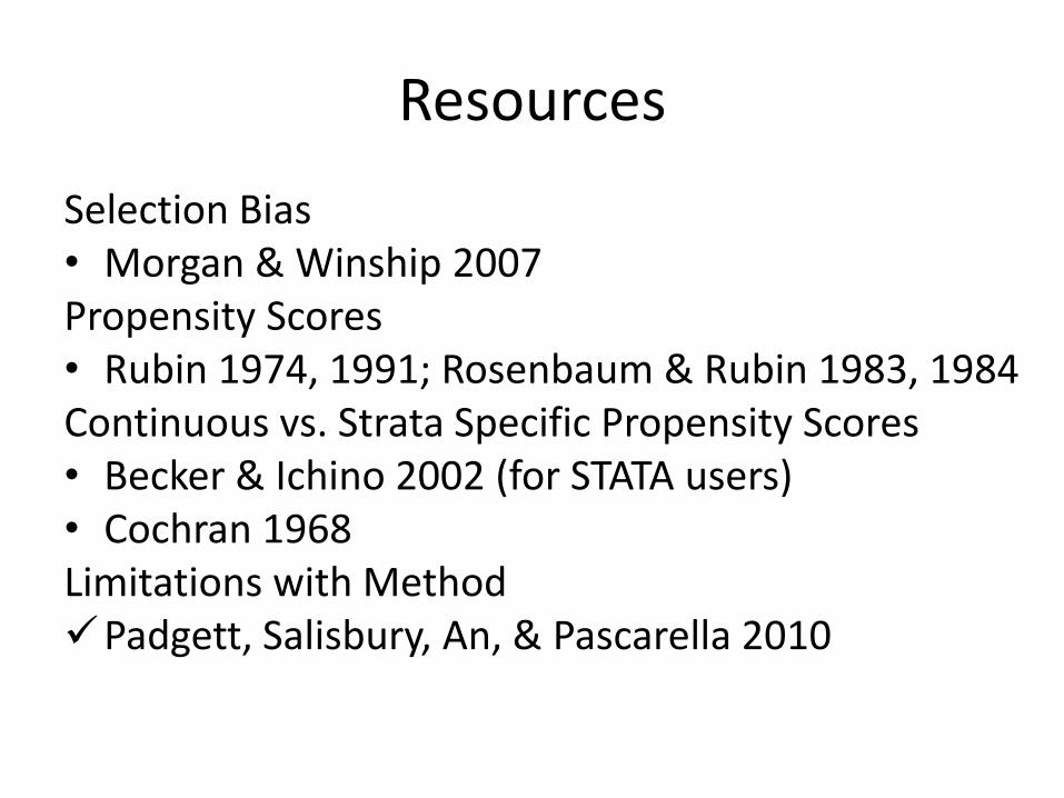
Resources

Selection Bias • Morgan & Winship 2007 Propensity Scores • Rubin 1974, 1991; Rosenbaum & Rubin 1983, 1984 Continuous vs. Strata Specific Propensity Scores • Becker & Ichino 2002 (for STATA users) • Cochran 1968 Limitations with Method Padgett, Salisbury, An, & Pascarella 2010

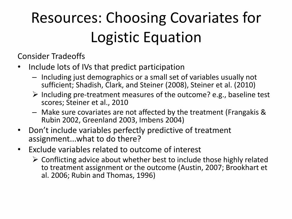
Resources: Choosing Covariates for Logistic Equation

Consider Tradeoffs • Include lots of IVs that predict participation

– Including just demographics or a small set of variables usually not sufficient; Shadish, Clark, and Steiner (2008), Steiner et al. (2010)

Including pre-treatment measures of the outcome? e.g., baseline test scores; Steiner et al., 2010

– Make sure covariates are not affected by the treatment (Frangakis & Rubin 2002, Greenland 2003, Imbens 2004)

• Don’t include variables perfectly predictive of treatment assignment...what to do there?

• Exclude variables related to outcome of interest Conflicting advice about whether best to include those highly related

to treatment assignment or the outcome (Austin, 2007; Brookhart et al. 2006; Rubin and Thomas, 1996)