ppl Internship report (Syed Wajih ul Hasnain)

1

Syed Wajih-ul-Hasnain [Internee]UNIVERSITY OF NEW SOUTH WALES (UNSW)

Internship Report 2015

INTERNSHIP REPORT

Reservoir Engineering Department

(5thJan., 2015 to 13th Feb., 2015)

P A K I S T A N P E T R O L E U M L I M I T E D

Submitted by:

Syed Wajih ul Hasnain

School of Petroleum Engineering

University of New South Wales (UNSW), Australia

1



Table of ContentsAcknowledgement 2

Introduction 3

Reservoir Department 4

Revision and Core Concepts 5

Fluid Properties 5

Material Balance 6

Primary Recovery Mechanism 6

Decline Curve Analysis 8

MBAL 10

Task Accomplished 11

Conclusion 20

1



Acknowledgement

I am very thankful to the Pakistan Petroleum Limited for providing me the opportunity to enhance my theoretical knowledge and experience the real time working environment.

I especially thank the Reservoir Engineering Department, PPL for giving me the chance to learn and clear my concepts. I am very grateful to Mr Adil Ahmed Siddiqui (senior reservoir engineer) who showed especial interest in grooming me by providing his precious time and by fine tuning my internship program.

Other people who I like to thank are:

1) Dr. Fareed Iqbal Siddiqui (Senior Manager Reservoir Engineering) 2) M. Noman Khan (Deputy Chief Engineer Reservoir)3) Mr Bilal Younus (Trainee Engineer)

1



1. Introduction:

The pioneer of the natural gas industry in the country, Pakistan Petroleum Limited (PPL) has been a frontline player in the energy sector since the mid-1950s. As a major supplier of natural gas, PPL today contributes over 20 percent of the country’s total natural gas supplies besides producing crude oil, Natural Gas Liquid and Liquefied Petroleum Gas.

The company’s history can be traced back to the establishment of a public limited company in June 1950, with majorshareholding by Burmah Oil Company (BOC) of the United Kingdom for exploration, prospecting, development and production of oil and natural gas resources. In September 1997, BOC disinvested from the Exploration and Production (E&P) sector worldwide and sold its equity in PPL to the Government of Pakistan (GoP). Subsequently, the government reduced its holding through an initial public offer in June 2004. More recently, GoP further disinvested its 5 percent shares, around 3.55 percent of the total paid-up capital, in PPL through Secondary Public Offering in 2014. Currently, the company’s shareholding is divided between the government, which owns about 68 percent, PPL Employees Empowerment Trust that has approximately 7 percent — being shares transferred to employees under BESOS — and private investors, who hold nearly 25 percent.

PPL operates six producing fields across the country at Sui (Pakistan’s largest gas field), Adhi, Kandhkot, Chachar,Mazarani and Hala and holds working interest in fifteen partner-operated producing fields, including Qadirpur the country’s second largest gas field.

As a major stakeholder in securing a safe energy future for the country, PPL pursues an aggressive exploration agenda aimed at enhancing hydrocarbon recovery and replenish reserves. PPL together with its subsidiaries has a portfolio of 47 exploration assets of which the company operates 27, including one contract in Iraq, while 20 blocks, comprising three offshore leases in Pakistan and two onshore concessions in Yemen, are operated by joint venture partners.

Over the years, PPL has developed a reliable foundation and infrastructure for providing clean and safe energy through sustainable exploitation of indigenous natural resources while adhering to best practices of corporate governance and employee health and safety and constraining the ecological footprint of its operations. As a result, Monitoring and Inspection, Design and Construction, Drilling and Well Engineering, Joint Operations, Operational Technical Support Services and Projects departments, Mazarani, Adhi and Kandhkot fields, Sui Field Gas Compressor Station, Sui Production, Sui Field Engineering and Sui Purification stand certified for ISO 9001 Quality Management System.

PPL has played a significant role as a responsible corporate citizen since the inception of its commercial activities inSui by establishing the Sui Model School in 1957 for children of workers and local communities.

1



2. Reservoir Department

Reservoir engineering department is the core department of PPL. All the important decisions and fact finding initial results regarding developing a field, reservoir management and surveillance are carried out here. The staff consists of highly qualified and well experienced professionals who are well qualified in their jobs.

Core Responsibilities:

Estimating reserves and forecasting for property evaluations and development planning. Carrying out reservoir simulation studies to optimize recoveries. Analyzing the properties of fluid to predict fluid behavior and various physical effects. Predicting reserves and performance for well proposals. Predicting and evaluating water-flood and enhanced recovery performance. Developing and applying reservoir optimization techniques. Developing cost-effective reservoir monitoring and surveillance programs. Performing reservoir characterization studies. Analyzing the economics and risk assessments of major development programs. Updating and booking of corporate reserves

1



3. Revision of Core Concepts:

On the recommendation of Sir Adil, I revised some basic concepts related to reservoir engineering which proved fruitful for the remaining of my internship.

3.1 Fluid Properties:

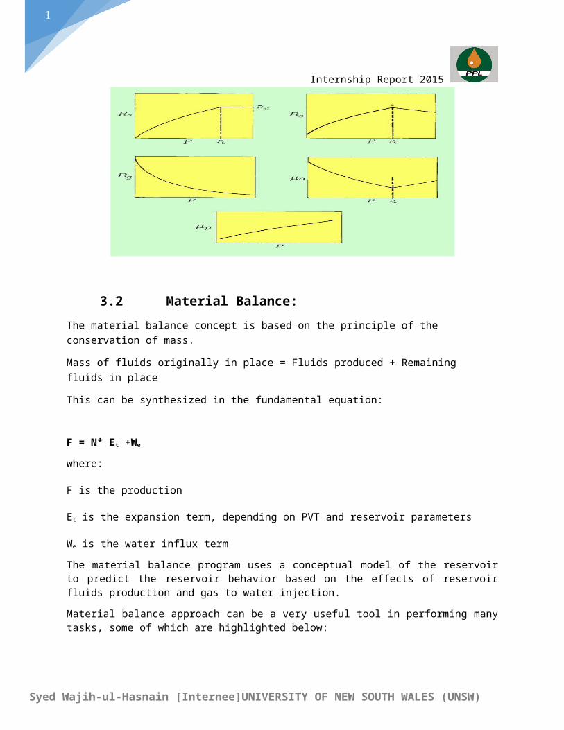
Oil Formation Volume Factor (Bo): The liquid-phase volume at reservoir conditions divided by the liquid volume of the same sample at standard conditions.

Gas Formation Volume Factor (Bg): The vapor-phase volume at reservoir conditions divided by the gas volume of the same sample at standard conditions.

Dissolved Gas-Oil Ratio (Rs): The ratio of the volume of surface gas to stock-tank oil in a reservoir liquid phase at reservoir conditions.

Dissolved Oil-Gas Ratio (Rv):The ratio of volume of stock tank oil to the surface gas contained in a reservoir vapor phase at reservoir conditions.

Two Phase Oil Formation Volume Factor (Bto): The total volume at reservoir conditions divided by its resulting oil-phase volume at standard conditions.

Two Phase Gas Formation Volume Factor (Btg): The total volume at reservoir conditions divided by its resulting gas-phase volume at standard conditions.

Expansivities: Total expansion of a unit mass of oil phase between two pressures at reservoir conditions.

1



3.2 Material Balance:

The material balance concept is based on the principle of the conservation of mass.

Mass of fluids originally in place = Fluids produced + Remaining fluids in place

This can be synthesized in the fundamental equation:

F = N* Et +We

where:

F is the production

Et is the expansion term, depending on PVT and reservoir parameters

We is the water influx term

The material balance program uses a conceptual model of the reservoir to predict the reservoir behavior based on the effects of reservoir fluids production and gas to water injection.

Material balance approach can be a very useful tool in performing many tasks, some of which are highlighted below:

·Quantify different parameters of a reservoir such as hydrocarbon in place, gas cap size, etc.

·Determine the presence, the type and size of an aquifer, encroachment angle, etc.

·Estimate the depth of the gas/oil, water/oil, gas/water contacts.

·Predict the reservoir pressure for a given production and/or injection schedule,

·Predict the reservoir performance and manifold back pressures for a given production schedule.

·Predict the reservoir performance and well production for a given manifold pressure schedule.

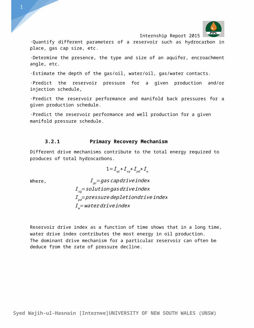
3.2.1 Primary Recovery Mechanism

Different drive mechanisms contribute to the total energy required to produces of total hydrocarbons.

1=I gc+ I sg+ I pd+ Iw

Where, I gc=gascapdrive indexI sg=solution gasdrive indexI pd=pressure depletiondrive indexIw=water driveindex

1



Reservoir drive index as a function of time shows that in a long time, water drive index contributes the most energy in oil production.The dominant drive mechanism for a particular reservoir can often be deduce from the rate of pressure decline.

1



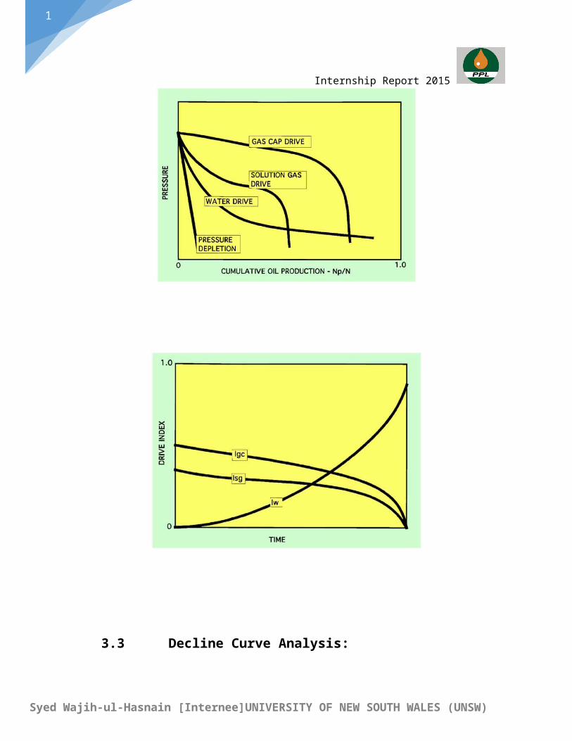
3.3 Decline Curve Analysis:

Decline curve analysis extrapolates past-performance observations to estimate future production performance.

As can be observed from the graph below, initial decline stage is sufficient to calculate future cumulative production and the amount of time requires producing oil which is very crucial considering the amount of money is at stake.

Below are the types of curves observes during the decline curve analysis:

1



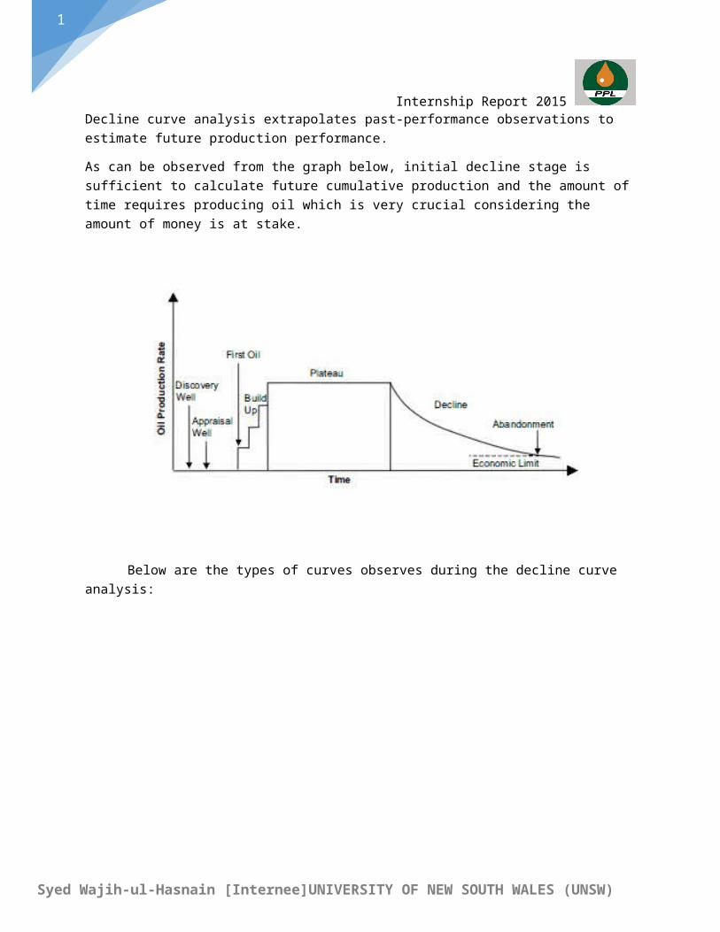
Steps for Decline Curve Analysis

Smooth the rate versus time data

Calculate D for each time increment by using D=−ln( q jq j−1 )/( t j−t j−1) Estimate Di and b from 1/d vs t plot Predict q and Np Match the actual and predicted values and reduce the error by iteration.

4. MBALMBAL is a reservoir modelling tool designed to allow for greater understanding of the current reservoir behavior and perform predictions while determining its depletion.

This is the tool which I focused on a lot. A good user of this software can attain very reliable results from it.

I tried to solve all the tasks given to me through this software to reconfirm my results.

1



5. Tasks Accomplished5.1 EstimatingOGIP by calculating pressure at datum depth provided Z factor and production data are given for the years 20005, 2007, 2011 and 2014.

K KBE

KBE, amsl

THF

THF, amsl

Sea Level

13.12 ft.

1



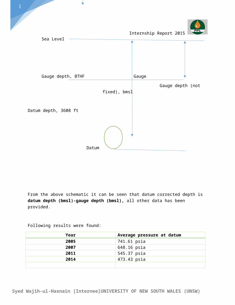
Gauge depth, BTHF Gauge

Gauge depth (not fixed), bmsl

Datum depth, 3608 ft

Datum

From the above schematic it can be seen that datum corrected depth is datum depth (bmsl)-gauge depth (bmsl), all other data has been provided.

Following results were found:

Year Average pressure at datum2005 741.61 psia2007 648.16 psia2011 545.37 psia2014 473.43 psia

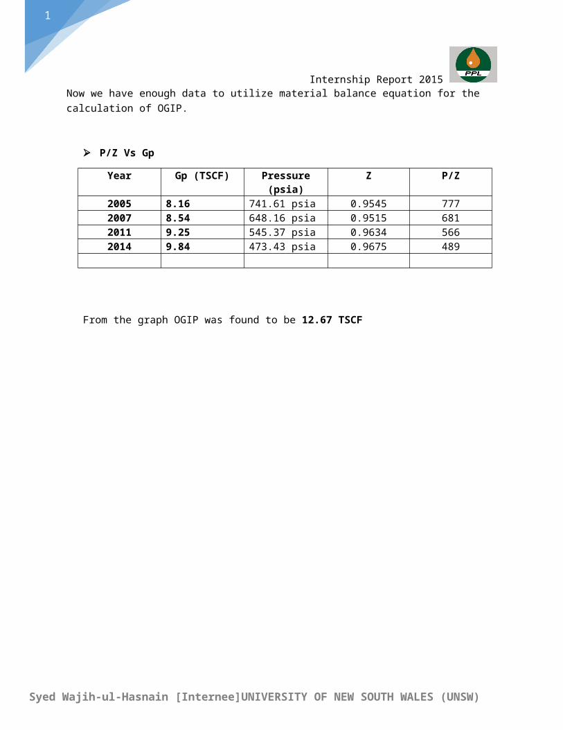
Now we have enough data to utilize material balance equation for the calculation of OGIP.

P/Z Vs Gp

Year Gp (TSCF) Pressure (psia) Z P/Z2005 8.16 741.61 psia 0.9545 7772007 8.54 648.16 psia 0.9515 6812011 9.25 545.37 psia 0.9634 5662014 9.84 473.43 psia 0.9675 489

1



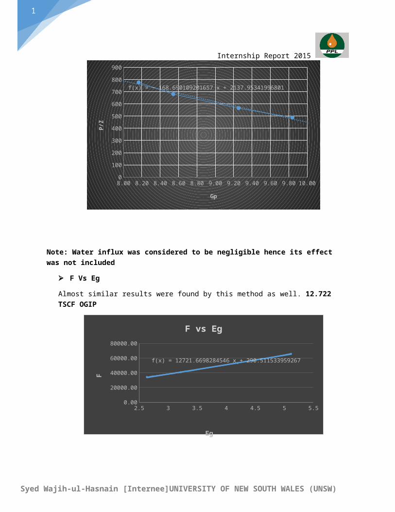
From the graph OGIP was found to be 12.67 TSCF

8.00 8.20 8.40 8.60 8.80 9.00 9.20 9.40 9.60 9.80 10.000

100

200

300

400

500

600

700

800

900

f(x) = − 168.690109201657 x + 2137.95341996801

Gp

P/Z

Note: Water influx was considered to be negligible hence its effect was not included

F Vs Eg

1


Internship Report 2015 Almost similar results were found by this method as well. 12.722 TSCF OGIP

2.5 3 3.5 4 4.5 5 5.50.00

10000.00

20000.00

30000.00

40000.00

50000.00

60000.00

70000.00

f(x) = 12721.6698284546 x + 290.511533959267

F vs Eg

Eg

F

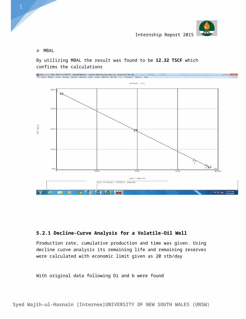
MBAL

By utilizing MBAL the result was found to be 12.32 TSCF which confirms the calculations

1



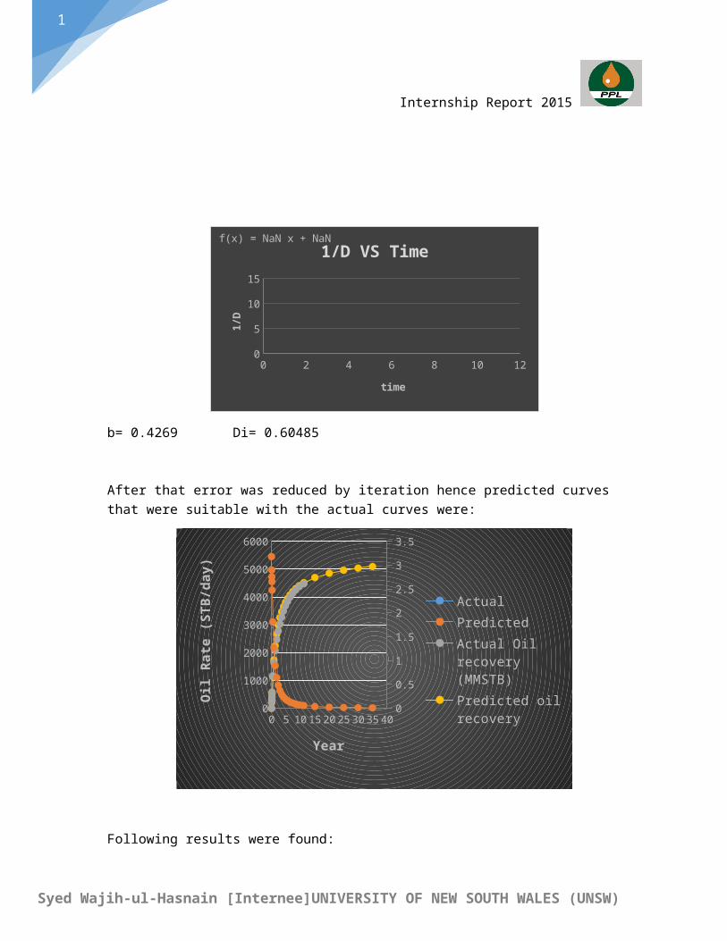
5.2.1 Decline-Curve Analysis for a Volatile-Oil Well

Production rate, cumulative production and time was given. Using decline curve analysis its remaining life and remaining reserves were calculated with economic limit given as 20 stb/day

With original data following Di and b were found

0 2 4 6 8 10 1202468

1012

f(x) = NaN x + NaN1/D VS Time

time

1/D

b= 0.4269 Di= 0.60485

After that error was reduced by iteration hence predicted curves that were suitable with the actual curves were:

1



0 5 10 15 20 25 30 35 400

1000

2000

3000

4000

5000

6000

0

0.5

1

1.5

2

2.5

3

3.5

ActualPredictedActual Oil recovery (MMSTB)Predicted oil recovery

Year

Oil

Rate

(STB

/day

)


b= 0.6 Di= 1.51 Reserves remaining (Np) = 311.893 MSTB Life remaining = 19.64 yrs

1



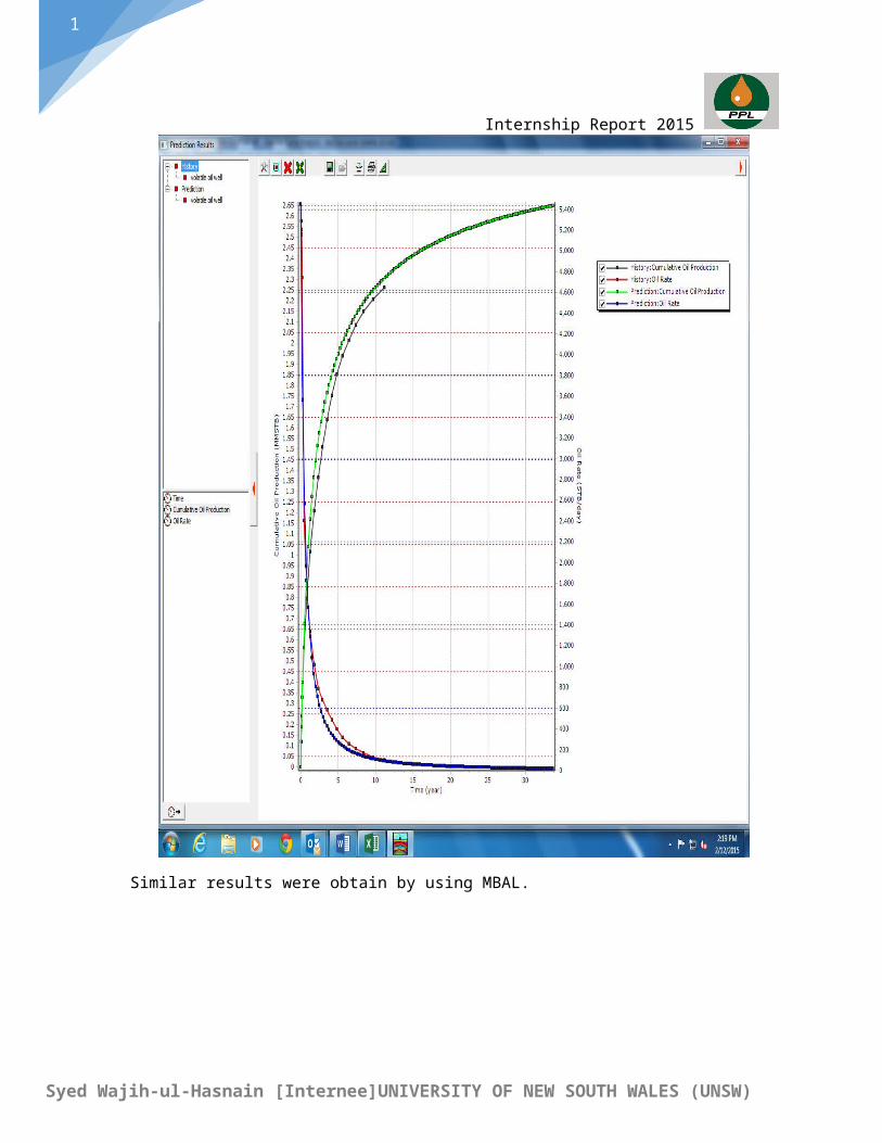
Similar results were obtain by using MBAL.

1



5.2.2 Decline-Curve Analysis for a Wet-Gas Well

Production rate, cumulative production and time was given. Using decline curve analysis its remaining life and remaining reserves were calculated with economic limit given as 1 MMscf/day

With original data following Di and b were found

0 0.5 1 1.5 2 2.5 3 3.5 4 4.50

0.5

1

1.5

2

2.5 2.28866077987281f(x) = 0.392672553819782 x + 0.997864861310077

1/D VS Time

Time (Years)

1/D

(Yea

rs)

b= 0.3927 Di= 1.0021


0 5 10 15 20 25 30 350 5 10 15 20 25 30 350

20000

40000

60000

80000

100000

120000

0

10

20

30

40

50

60

70

Gas rate Predicted gas rateCumulative production Predicted cumulative production

Time (Years)

Gas r

ate

(Msc

f/da

y)

1




b= 0.46 Di= 1.0021 Reserves remaining (Np) = 14.31 Bscf Life remaining = 12.00 yrs


5.2.3 Decline-Curve Analysis for a Wet-Gas Well

Production rate, cumulative production and time were given. Using decline curve analysis its remaining life and remaining reserves were calculated with economic limit given as 4 STB/day

1


Internship Report 2015 With original data following Di and b were found

0 2 4 6 8 10 12 14 16 180

2

4

6

8

10

12f(x) = NaN x + NaN

b= 0.2097 Di= 0.2318


0 10 20 30 40 50 600 10 20 30 40 50 600

50

100

150

200

250

300

350

0

100

200

300

400

500

600

Chart Title

Oil rate predicted oil ratecumulative production predicted cumulative production

time (Years)

Oil

rate

(stb

/day

)


1


Internship Report 2015 b= 0.27 Di= 0.286 Reserves remaining (Np) = 37.53 MSTB Life remaining = 14.19 yrs


6) ConclusionThe internship at Reservoir Engineering Department has been a good learning experience. I learnt a lot from the professionals of the pioneer Petroleum Company of Pakistan. I thank everyone for giving me their valuable time and sharing precious knowledge with me. Learning software and working on real problems have definitely enhanced my knowledge.

I hope this internship will help me develop my future career.

ppl Internship report (Syed Wajih ul Hasnain)

Documents

Transcript of ppl Internship report (Syed Wajih ul Hasnain)