PPL ATH Vol. 77, No. 6, pp. 2093{2118

Copyright © by SIAM. Unauthorized reproduction of this article is prohibited.

SIAM J. APPL. MATH. c© 2017 Society for Industrial and Applied MathematicsVol. 77, No. 6, pp. 2093–2118

STABLE EQUILIBRIA OF ANISOTROPIC PARTICLESON SUBSTRATES: A GENERALIZEDWINTERBOTTOM CONSTRUCTION∗

WEIZHU BAO† , WEI JIANG‡ , DAVID J. SROLOVITZ§ , AND YAN WANG¶

Abstract. We present a new approach for predicting stable equilibrium shapes of two-dimensionalcrystalline islands on flat substrates, as commonly occur through solid-state dewetting of thin films.The new theory is a generalization of the widely used Winterbottom construction (i.e., an extensionof the Wulff construction for particles on substrates). This approach is equally applicable to caseswhere the crystal surface energy is isotropic, weakly anisotropic, strongly anisotropic, and “cusped”.We demonstrate that, unlike in the classical Winterbottom approach, multiple equilibrium islandshapes may be possible when the surface energy is strongly anisotropic. We analyze these shapesthrough perturbation analysis, by calculating the first and second variations of the total free energyfunctional with respect to contact locations and island shape. Based on this analysis, we find thenecessary conditions for the equilibria to be stable to two-dimensional perturbations and exploit thisthrough a generalization of the Winterbottom construction to identify all possible stable equilibriumshapes. Finally, we propose a dynamical evolution method based on surface diffusion mass transportto determine whether all of the stable equilibrium shapes are dynamically accessible. Applyingthis approach, we demonstrate that islands with different initial shapes may evolve into differentstationary shapes and show that these dynamically determined stationary states correspond to thepredicted stable equilibrium shapes, as obtained from the generalized Winterbottom construction.

Key words. solid-state dewetting, generalized Winterbottom construction, thermodynamicvariation, multiple stable equilibrium, anisotropic surface energy, surface diffusion

AMS subject classifications. 74G65, 74G15, 74H55, 74G99

DOI. 10.1137/16M1091599

1. Introduction. Many micro- and nanoscale devices use solid thin films as ba-sic building components. Compared to traditional bulk materials, thin films have avery large surface-area-to-volume ratio. Such films can be unstable to particle forma-tion (dewetting or agglomeration) due to surface tension/capillarity effects, especiallyat high temperatures and/or on long time scales. Solid-state dewetting has beenobserved and studied in a large number of experimental systems (e.g., see the recentreview papers [26, 39]), such as Ni films on MgO substrates and Si films on amorphousSiO2 substrates (i.e., SOI).

∗Received by the editors August 29, 2016; accepted for publication (in revised form) June 8, 2017;published electronically November 28, 2017.

http://www.siam.org/journals/siap/77-6/M109159.htmlFunding: The first author’s work was supported by the Singapore A*STAR SERC PSF grant

1321202067. The second author’s work was supported by National Natural Science Foundationof China 11401446 and 91630313. The third author’s work was supported by the NSF Divisionof Materials Research through award DMR 1609267. The fourth author’s work was supported byNational Natural Science Foundation of China 91630207 and U1530401, and China PostdoctoralScience Foundation 2017M610750.†Department of Mathematics, National University of Singapore, Singapore 119076 (matbaowz@

nus.edu.sg).‡Corresponding author. School of Mathematics and Statistics and Computational Science Hubei

Key Laboratory, Wuhan University, Wuhan 430072, People’s Republic of China ([email protected]).§Departments of Materials Science and Engineering and Mechanical Engineering and Applied

Mechanics, University of Pennsylvania, Philadelphia, PA 19104 ([email protected]).¶Applied and Computational Mathematics Division, Beijing Computational Science Research

Center, Beijing 100193, People’s Republic of China ([email protected]).

2093

Dow

nloa

ded

11/3

0/17

to 2

02.1

14.7

0.14

3. R

edis

trib

utio

n su

bjec

t to

SIA

M li

cens

e or

cop

yrig

ht; s

ee h

ttp://

ww

w.s

iam

.org

/jour

nals

/ojs

a.ph

p

http://www.siam.org/journals/siap/77-6/M109159.html

mailto:[email protected]







2094 W. BAO, W. JIANG, D. J. SROLOVITZ, AND Y. WANG

The dewetting of solid thin films is similar to the dewetting of liquid films [3,35, 46]. The main difference between solid and liquid dewetting is associated withanisotropy of physical properties (e.g., surface energy, diffusivity) and the mode ofmass transport; solid-state dewetting is usually dominated by surface diffusion ratherthan fluid dynamics (as in liquid-state dewetting). Solid-state dewetting is increas-ingly important in many modern technologies where it can be either detrimental oradvantageous. For example, dewetting can destroy micro-/nanodevice performancethrough instabilities in carefully patterned structures (this is a major reliability is-sue). On the other hand, dewetting of a continuous film can be used to createpatterns of nanoscale particles which can be used for sensors [30], for optical andmagnetic devices [1], and as catalysts for the growth of carbon or semiconductornanowires [36]. Therefore, solid-state dewetting is attracting ever more attention(e.g., see [5, 15, 17, 33, 34, 37, 44, 50]).

From a mathematical perspective, theoretical solid-state dewetting studies can becategorized into two major classes. The first focuses on the equilibrium of particles onsubstrates (e.g., [22, 49]), i.e., finding the stable equilibrium shapes of solid-state par-ticles via constrained minimization; the second examines the temporal evolution of thefilm/particle morphology (e.g., [5, 15, 16, 37, 41, 44]), i.e., examining dewetting dy-namics subject to different classes of kinetic phenomena, such as Rayleigh-like instabil-ities [15, 18], corner-induced instabilities [50], and periodic mass-shedding [41, 44]. Inthis paper, we mainly focus on the determination of equilibrium shapes of anisotropicparticles on substrates and validate the theoretical predictions on (multiple) stableequilibria by numerically solving sharp-interface dynamical evolution models basedon surface diffusion and contact line migration.

Following the thermodynamic principles laid out by Gibbs [9], we seek to deter-mine the equilibrium shape of an island/film on a substrate that is a connected shapeΩ which minimizes the total interfacial energy functional of the system [16, 22],

minΩ

W =∫

ΓFVγFV dΓFV +

∫ΓFS

γFSdΓFS +∫

ΓV SγV SdΓV S︸︷︷︸

Substrate Energy

s.t. |Ω| = const.(1.1)

Here, Ω refers to the island/film (see Figure 1), |Ω| represents its total volume(three dimensions)/area (two dimensions) of the region, ΓFV , ΓFS, and ΓV S repre-sent the film/vapor, film/substrate, and vapor/substrate interfaces, respectively, andγFV , γFS, γV S represent their corresponding interfacial energy densities. As is typical

Fig. 1. A schematic illustration of a film or island on a flat, rigid substrate in two dimen-sions with three interfaces, i.e., film/vapor (FV), film/substrate (FS), and vapor/substrate (VS)interfaces.

Dow

nloa

ded

11/3

0/17

to 2

02.1

14.7

0.14

3. R

edis

trib

utio

n su

bjec

t to

SIA

M li

cens

e or

cop

yrig

ht; s

ee h

ttp://

ww

w.s

iam

.org

/jour

nals

/ojs

a.ph

p


STABLE EQUILIBRIA OF ANISOTROPIC PARTICLES 2095

in solid-state dewetting problems, we assume that γFS and γV S are constants (weassume here that the substrate is flat and remains so during the entire dewettingprocess, but the effects of a mechanically or chemically reactive substrate also canbe included in the model). If γFV is a constant, the problem is isotropic; if γFV de-pends on the orientation of the film/vapor interface (free surface), it is anisotropic.For crystalline films, γFV is a function of the surface normal (the angle between theouter surface normal and the y-axis in two dimensions) θ of the film/vapor interface,i.e., γFV := γ(θ) ∈ C0[−π, π] is a positive periodic function. For γ(θ) ∈ C2[−π, π],the surface energy is referred to as smooth; otherwise, it is nonsmooth or “cusped”.For a smooth surface energy γ(θ), it is weakly anisotropic if the surface stiffnessγ(θ) := γ(θ) + γ ′′(θ) > 0 ∀ θ ∈ [−π, π]; otherwise, it is strongly anisotropic. Weremark here that in the strongly anisotropic case, one approach in the literature is to“modify” the surface energy γ(θ) such that γ(θ) is positive ∀ θ ∈ [−π, π] [6, 7].

In the absence of a substrate, the island/film is completely surrounded by thevapor and the problem reduces to the classical problem in applied mathematics andmaterials science, i.e., determining a connected shape Ω such that

minΩ

W =∫

ΓFVγFV dΓFV for |Ω| = const.(1.2)

This problem was first solved by Wulff [45] over a century ago using a geometricalapproach which has become known as the Wulff (or Gibbs–Wulff) construction (seean illustration in Figure 2). In fact, for the isotropic and weakly anisotropic cases,the Wulff envelope yields a unique connected particle shape which is the equilibrium;however, for the strongly anisotropic case, the Wulff envelope includes distinct “ears”,and its inner simply connected envelope yields the equilibrium by applying the vanGogh treatment, i.e., cutting off/removing these “ears” (cf. Figure 2(c)). For theconvenience of readers, Figure 3 displays the Wulff constructions for several differenttypes of surface energy densities γ(θ).

Subsequently, several researchers (e.g., see [8, 25, 27, 31, 38]) provided rigorousproofs that the Wulff construction indeed yields a particle shape of minimal energy,i.e., the solution of (1.2). For example, Fonseca and Muller [8] applied geometricmeasure theory to show that the Wulff construction gives the equilibrium (solution)to (1.2). On the other hand, Gurski, McFadden, and Miksis determined the linear

θ

γ (θ )

(a) γ−plot (b) Draw normals(c) Inner envelope =

equilibrium shape

Fig. 2. A schematic illustration for the Wulff construction in two dimensions with a stronglyanisotropic surface energy γ(θ) = 1 + 0.3 cos(4θ), where (a) is the γ-plot (blue curve of pointswith angle θ and distance γ(θ) to the origin, i.e., the Wulff point) with the gray line (normal)perpendicular to the radius vector; (b) shows these normals at all points along the γ-plot; (c) showsthe equilibrium particle (Wulff) shape in blue (i.e., the solution to (1.2))—this is the inner envelopeof all of these planes (outlined in black) after the “ears” have been removed.

Dow

nloa

ded

11/3

0/17

to 2

02.1

14.7

0.14

3. R

edis

trib

utio

n su

bjec

t to

SIA

M li

cens

e or

cop

yrig

ht; s

ee h

ttp://

ww

w.s

iam

.org

/jour

nals

/ojs

a.ph

p



(a) (b) (c) (d)

Fig. 3. γ-plot (blue line), Wulff envelope (black line) and Wulff shape (shaded blue region) forseveral typical surface energy densities γ(θ): (a) γ(θ) ≡ 1 (isotropic); (b) γ(θ) = 1 + 0.06 cos(4θ)(weakly anisotropic); (c) γ(θ) = 1+0.3 cos(4θ) (strongly anisotropic); and (d) γ(θ) = | cos θ|+ | sin θ|(“cusped”).

stability of the above problem under the weak anisotropy, and they considered firstand second variations of a two-dimensional (2D) equilibrium shape, while includingthe important effects of an axial perturbation (i.e., Rayleigh instability) [10, 11]. Infact, the variational problem (1.2) is scale-invariant and thus it can be first solvedfor any fixed volume/area in three/two dimensions and followed by an appropriaterescaling. In two dimensions, if γ(θ) ∈ C1[−π, π], the Wulff envelope can be expressedanalytically as [14, 32, 41]

x(θ) = −γ(θ) sin θ − γ ′(θ) cos θ,y(θ) = γ(θ) cos θ − γ ′(θ) sin θ,

θ ∈ [−π, π],(1.3)

where a scaling factor can be chosen such that the area of the inner simply connectedregion surrounded by the curve is |Ω|.

The equilibrium shape of an island on a substrate (i.e., the island in contact witha flat substrate where the substrate energy terms are included) is the solution to (1.1)and can be determined using the geometrical Wulff–Kaischew construction [19]. Thisequilibrium shape is often called the Winterbottom shape [43], i.e., a Wulff shapetruncated by a flat substrate plane/line in three/two dimensions, and where the Wulffshape is truncated depends on the wettability of the substrate, i.e., γV S − γFS. TheWinterbottom construction, though widely studied and applied (e.g., [21, 23, 48]),only describes island shapes corresponding to the global minimum of the free energy,i.e., the solution to (1.1). It does not, however, predict all possible stable equilibria,including metastable solutions—local minimizers. In fact, experiments often showisland shapes that are not consistent with the Winterbottom shape and this dis-crepancy is likely attributable to the island shapes trapped in metastable free energyminima [24, 28]. To clarify this issue, this paper addresses the determination of all pos-sible stable equilibria (including local and global minimizers) of the problem (1.1). Wepropose a generalization of the Winterbottom construction that not only is simply thetruncated Wulff shape but also considers the “ears” from the truncated Wulff envelope.

This paper is organized as follows. In section 2, we consider first-order pertur-bations to the shape of the 2D film/vapor interface and contact positions, including

Dow

nloa

ded

11/3

0/17

to 2

02.1

14.7

0.14

3. R

edis

trib

utio

n su

bjec

t to

SIA

M li

cens

e or

cop

yrig

ht; s

ee h

ttp://

ww

w.s

iam

.org

/jour

nals

/ojs

a.ph

p



the first and second thermodynamic variations of the total interfacial energy func-tional. Based on the thermodynamic variations, in section 3 we propose a generalizedWinterbottom construction for determining all possible stable equilibrium shapes. Insection 4, we adopt a sharp-interface dynamical evolution model under surface diffu-sion and contact line migration for simulating solid-state dewetting and implementthis model by a numerical method from different initial conditions for finding stableequilibrium shapes of the problem. Then, several numerical simulations are reportedto validate the generalized Winterbottom construction in section 5. Finally, we drawsome conclusions in section 6.

2. Thermodynamic variation. In this section, we consider the solid-statedewetting problem in two dimensions and calculate its first and second thermody-namic variations of the total free energy of the system. For simplicity, all the physi-cal variables in the following discussion are nondimensionalized, and the subscript sstands for differentiation with respect to the arc length.

As illustrated in Figure 4, the film/vapor interface is denoted as Γ := X(s) =(x(s), y(s)), s ∈ [0, L] with arc length s, and L represents the total length of theinterface Γ. The outer unit normal vector n and unit tangent vector τ can be expressedas n = (−ys, xs) and τ = (xs, ys). Suppose that the flat substrate coincides with thex-axis of a Cartesian system, and xlc and xrc represent the x-axis coordinates of the leftand right contact points, respectively, i.e., x(0) = xlc and x(L) = xrc . In this scenario,the constrained minimization problem (1.1) can be reformulated as (by subtracting aconstant and in dimensionless form)

minΩ

W := W (Γ) =∫

Γγ(θ) dΓ− σ(xrc − xlc) s.t. |Ω| = const.,(2.1)

where σ := (γV S−γFS)/γ0 is a dimensionless material constant, γ0 is a surface energydensity employed to nondimensionalize the equations, and γ(θ) is the dimensionlessfilm/vapor surface energy density (scaled by γ0). In the following discussion, accordingto (1.3), we assume that γ(θ) ∈ C3([−π, π]) so that the equilibrium curve is at leasta continuous piecewise-C2 curve.

2.1. First and second variations. We calculate the first and second variationsof the energy functional W defined in (2.1) with respect to the interface curve Γ andthe left and right contact points, xlc and xrc . In general, the calculation of the first vari-ation with respect to a closed curve, such as the functional defined in the problem (1.2)[4] and the Willmore functional [42], only requires consideration of the perturbationalong the normal direction of the closed curve, because the perturbation along the tan-gent direction of the closed curve contributes nothing to the first variation. However,in this case, the energy functional also depends on the two contact points (xlc and xrc),and we find that the tangent perturbation plays an important role in understandingcontact point perturbations; hence, tangent perturbation must also be included.

We assume that the interface Γ = (x(s), y(s)) is a continuous piecewise-C2 curve,and its derivatives about the arc length, in the following discussion, can be understoodin the weak sense. We consider the following infinitesimal first-order perturbationabout the curve Γ along both its normal and tangent directions (see Figure 4):

Γε = Γ + εϕ(s)n + εψ(s)τ ,(2.2)

where 0 < ε 1 is a small perturbation parameter, and ϕ(s), ψ(s) ∈ Lip[0, L]represent Lipschitz continuous perturbation functions with respect to arc length s.

Dow

nloa

ded

11/3

0/17

to 2

02.1

14.7

0.14

3. R

edis

trib

utio

n su

bjec

t to

SIA

M li

cens

e or

cop

yrig

ht; s

ee h

ttp://

ww

w.s

iam

.org

/jour

nals

/ojs

a.ph

p



Film

Substrate

Vapor

x lc

x rc

Γτ

n

θ

Γǫ = Γ + ǫϕ(s)n + ǫψ (s)τ

Fig. 4. A schematic illustration of an infinitesimal perturbation (denoted by the dashed line)about the film/vapor interface curve Γ along its normal and tangent directions. As the curve isperturbed, the contact points xl

c and xrc may move along the substrate.

Then the two components of the new curve Γε can be expressed as follows:

Γε = (xε(s), yε(s)) = (x(s) + εu(s), y(s) + εv(s)), 0 ≤ s ≤ L,(2.3)

where s is still a parameterization (but not the arc length) of the new curve Γε andits two component increments along the x- and y-axes are defined as

u(s) = xs(s)ψ(s)− ys(s)ϕ(s),v(s) = xs(s)ϕ(s) + ys(s)ψ(s).

(2.4)

Equivalently, the functions ϕ(s) and ψ(s) can be expressed byϕ(s) = xs(s)v(s)− ys(s)u(s),ψ(s) = xs(s)u(s) + ys(s)v(s).

(2.5)

As illustrated in Figure 4, because the contact points must move along the substrate,the increments along the y-axis at the two contact points must be zero, i.e.,

v(0) = v(L) = 0 ⇐⇒ xs(0)ϕ(0) + ys(0)ψ(0) = xs(L)ϕ(L) + ys(L)ψ(L) = 0.(2.6)

Due to this infinitesimal perturbation, the total interface free energy W (Γε) :=W (Γε;ϕ,ψ) for the new curve Γε after perturbation becomes

W (Γε) := W (Γε;ϕ,ψ) =∫

Γεγ(θε) dΓε − σ

[(xrc + εu(L)

)−(xlc + εu(0)

)]=∫ L

0γ

(arctan

yεsxεs

)√(xεs)2 + (yεs)2 ds− σ

[(xrc + εu(L)

)−(xlc + εu(0)

)],(2.7)

where yεs = ys + εvs and xεs = xs + εus, θε := arctan yεsxεs∈ [−π, π], and the function

“arctan” is the generalization of the usual arctangent function [16].If the total energy W (Γε) is understood as a function of the perturbation param-

eter ε, then by simple calculations, we obtain

dW (Γε)dε

=∫ L

0

[γ ′(θε)

dθε

dε

√(xεs)2 + (yεs)2 + γ(θε)

xsus + ysvs + ε(u2s + v2

s)√(xεs)2 + (yεs)2

]ds

−σ[u(L)− u(0)

],(2.8)

Dow

nloa

ded

11/3

0/17

to 2

02.1

14.7

0.14

3. R

edis

trib

utio

n su

bjec

t to

SIA

M li

cens

e or

cop

yrig

ht; s

ee h

ttp://

ww

w.s

iam

.org

/jour

nals

/ojs

a.ph

p



wheredθε

dε=

xsvs − ysus(xεs)2 + (yεs)2 .(2.9)

Noting (2.4), (2.8), and (2.9), we can calculate the rate of change of the total interfaceenergy functional with respect to the curve Γ in terms of ε as

δW (Γ;ϕ,ψ) = limε→0

W (Γε)−W (Γ)ε

=dW (Γε)dε

∣∣∣ε=0

=∫ L

0

[γ ′(θ)(ϕs − κψ) + γ(θ)κϕ+ γ(θ)ψs

]ds− σ

[u(L)− u(0)

]=(γ ′(θ)ϕ

)∣∣∣s=Ls=0

+∫ L

0γ ′′(θ)κϕ ds−

∫ L

0γ′(θ)κψ ds+

∫ L

0γ(θ)κϕ ds

+(γ(θ)ψ

)∣∣∣s=Ls=0

+∫ L

0γ ′(θ)κψ ds− σ

[u(L)− u(0)

]=∫ L

0

(γ ′′(θ) + γ(θ)

)κϕ ds+

[γ ′(θ)ϕ(s) + γ(θ)ψ(s)− σu(s)

]s=Ls=0

,(2.10)

where δW (Γ;ϕ,ψ) is called the first variation of the interface energy functional (2.1)and κ represents the curvature of the curve, i.e., κ = −yssxs + xssys.

Assume that θla and θra are contact angles at the left and right contact points,respectively; then we have

xs(0) = cos θla, ys(0) = sin θla, xs(L) = cos θra, ys(L) = sin θra.(2.11)

From (2.5) and (2.6), we haveψ(0) = u(0) cos θla, ϕ(0) = −u(0) sin θla,ψ(L) = u(L) cos θra, ϕ(L) = −u(L) sin θra.

(2.12)

Inserting (2.12) into (2.10), we obtain

δW (Γ;ϕ,ψ) =∫ L

0µ(s)ϕ(s) ds+ f(θra;σ)u(L)− f(θla;σ)u(0),(2.13)

where

f(θ;σ) := γ(θ) cos θ − γ ′(θ) sin θ − σ,(2.14)

and µ := µ(s) represents the dimensionless chemical potential of the system,

µ(s) := γ(θ)κ(s) =(γ ′′(θ) + γ(θ)

)κ(s),(2.15)

and θ := θ(s) is the local orientation of the interface curve.Similar to the first variation, we calculate the second variation of the energy

functional (2.1). From (2.8) and (2.9), we have

d2W (Γε)dε2

=∫ L

0

γ ′′(θε)

(dθεdε

)2√(xεs)2 + (yεs)2 + γ ′(θ)

d2θε

dε2

√(xεs)2 + (yεs)2

+ 2γ ′(θε)dθε

dε

xsus + ysvs + ε(u2s + v2

s)√(xεs)2 + (yεs)2

+ γ(θε)u2s + v2

s√(xεs)2 + (yεs)2

− γ(θε)

[xsus + ysvs + ε(u2

s + v2s)]2[

(xεs)2 + (yεs)2]3/2

ds,(2.16)

Dow

nloa

ded

11/3

0/17

to 2

02.1

14.7

0.14

3. R

edis

trib

utio

n su

bjec

t to

SIA

M li

cens

e or

cop

yrig

ht; s

ee h

ttp://

ww

w.s

iam

.org

/jour

nals

/ojs

a.ph

p



where xεs = xs + εus, yεs = ys + εvs, and dθε

dε is defined in (2.9) and

d2θε

dε2= −2

(xsvs − ysus)[xsus + ysvs + ε(u2

s + v2s)]

[(xεs)2 + (yεs)2

]2 .(2.17)

Substituting (2.5) and (2.17) into (2.16) and recalling that κ = −yssxs + xssys andx2s + y2

s = 1, we obtain

δ2W (Γ;ϕ,ψ) =d2W (Γε)dε2

∣∣∣ε=0

=∫ L

0

γ ′′(θ)(xsvs − ysus)2 + γ(θ)

[(u2s + v2

s

)− (xsus + ysvs)2] ds

=∫ L

0

[γ(θ) + γ ′′(θ)

](xsvs − ysus)2 ds =

∫ L

0γ(θ)

(ϕs − κψ

)2ds.(2.18)

2.2. Equilibrium shapes and stability. Based on the above first variation ofthe total free energy functional, i.e., (2.13), and by assuming the normal perturbationfunction ϕ(s) satisfies ∫ L

0ϕ(s) ds = 0(2.19)

to ensure the total area/mass conservation in the first-order sense, we obtain nec-essary and sufficient conditions for equilibrium shapes of the solid-state dewettingproblem (2.1).

Definition 2.1 (equilibrium shapes). If a continuous piecewise-C2 curve Γe :=(x(s), y(s)

)for s ∈ [0, L] satisfies δW (Γe;ϕ,ψ) ≡ 0 ∀ ϕ,ψ ∈ Lip[0, L] with the

perturbation function ϕ(s) satisfying (2.19), i.e.,∫ L

0 ϕ(s) ds = 0, it is an equilibriumshape of the solid-state dewetting problem (2.1).

Lemma 2.2. Assume that a continuous piecewise-C2 curve Γe :=(x(s), y(s)

)for

s ∈ [0, L] represents the film/vapor interface of the solid-state dewetting problem (2.1)with material constant σ and surface energy density γ(θ). Then Γe is an equilibriumshape if and only if the following two conditions are satisfied:

µ(s) := γ(θ)κ(s) = [γ(θ) + γ ′′(θ)]κ(s) ≡ C, a.e. s ∈ [0, L],(2.20)f(θ;σ) = γ(θ) cos θ − γ ′(θ) sin θ − σ = 0, θ = θla, θ

ra,(2.21)

where the constant C is determined by the given area of the film, and θla ∈ [0, π] andθra ∈ [−π, 0] represent the left and right contact angles of Γe, respectively.

Proof. It’s easy to see that if the conditions (2.20)–(2.21) are both satisfied, by us-ing (2.13) and (2.19), then we find that δW (Γe;ϕ,ψ) ≡ 0 ∀ϕ,ψ ∈ Lip[0, L]. Therefore,Γe is an equilibrium shape.

Conversely, if Γe is an equilibrium shape, then δW (Γe;ϕ,ψ) ≡ 0 ∀ϕ,ψ ∈ Lip[0, L].Since u(0) and u(L) are arbitrary, by using (2.13), we can obtain the condition (2.21)and the following expression: ∫ L

0µ(s)ϕ(s) ds = 0.

Dow

nloa

ded

11/3

0/17

to 2

02.1

14.7

0.14

3. R

edis

trib

utio

n su

bjec

t to

SIA

M li

cens

e or

cop

yrig

ht; s

ee h

ttp://

ww

w.s

iam

.org

/jour

nals

/ojs

a.ph

p



By choosing C = 1L

∫ L0 µ(s) ds and making use of

∫ L0 ϕ(s) ds = 0, we have

∫ L0

(µ(s)−

C)ϕ(s) ds = 0. By choosing ϕ(s) = µ(s)− C, we obtain∫ L

0

(µ(s)− C

)2ds = 0.

Therefore, we find that µ(s) ≡ C, a.e. s ∈ [0, L], i.e., the condition (2.20).

It can be easily shown that the Wulff envelope, i.e., (1.3), satisfies the condition(2.20): µ(s) ≡ C. Note that when γ(θ) is strongly anisotropic, the curve givenabove by (1.3) will self-intersect, i.e., the Wulff envelope will form “ears”. In thiscase, without considering the substrate energy, the Wulff construction states thatcutting off all “ears” will give the unique equilibrium shape. Considering the substrateenergy, the (classical) Winterbottom construction still follows the Wulff constructionapproach; however, in the following we show that this is not always true.

Condition (2.21) is called the anisotropic Young equation, which has been de-rived over the years by many authors (e.g., see [13, 29, 41]). Its roots determine theanisotropic Young angles, θa ∈ [−π, π]. For the isotropic case, i.e., γ(θ) ≡ 1, it is easyto see that the anisotropic Young equation collapses to the well-known (isotropic)Young equation, i.e., cos θ = σ = γV S−γFS

γ0, which is commonly used in liquid-state

wetting/dewetting [47, 3]. When −1 ≤ σ ≤ 1, the Young equation has a unique rootθla = cos−1 σ in the interval [0, π] and a unique root θra = − cos−1 σ in the interval[−π, 0], and when |σ| > 1, there is no root and complete wetting or dewetting occurs.For the anisotropic case, differentiating f(θ;σ) with respect to θ, we obtain

df(θ;σ)dθ

= −[γ ′′(θ) + γ(θ)] sin θ = −γ(θ) sin θ, θ ∈ [−π, π].

For the weakly anisotropic case, i.e., the surface stiffness γ(θ) = γ ′′(θ) + γ(θ) > 0for θ ∈ [−π, π], f(θ;σ) is a monotonously decreasing function on the interval [0, π]and a monotonously increasing function on the interval [−π, 0], respectively; in thiscase, for any given σ ∈ R, the anisotropic Young equation (2.21) has at most one rootθ = θla ∈ [0, π] and at most one root θ = θra ∈ [−π, 0], respectively. On the other hand,in the strongly anisotropic case, i.e., the surface stiffness γ(θ) = γ ′′(θ) +γ(θ) changessign over [−π, π] and the anisotropic Young equation (2.21) may have multiple rootsover the interval [0, π] (see Figure 5) and/or over the interval [−π, 0].

Looking back at the explicit expression of the Wulff envelope, i.e., (1.3), if we firstuse a flat substrate line given by the expression y = σ to truncate the Wulff envelope

0 0.2 0.4 0.6 0.8 1−1

0

1

2

θ/π

f(θ;

σ)

β = 0β = 0.06β = 0.15β = 0.3

Fig. 5. Plot of f(θ;σ) as a function of θ for γ(θ) = 1 + β cos(4θ) for different β and σ = −0.5.

Dow

nloa

ded

11/3

0/17

to 2

02.1

14.7

0.14

3. R

edis

trib

utio

n su

bjec

t to

SIA

M li

cens

e or

cop

yrig

ht; s

ee h

ttp://

ww

w.s

iam

.org

/jour

nals

/ojs

a.ph

p



and then redefine the origin of the Cartesian coordinates for the Wulff envelope bydenoting the y-coordinate of the flat substrate line as the zero (the x-coordinate isunchanged), we find that the substrate intersects the Wulff envelope at contact points(x(θla), 0) and (x(θra), 0) with contact angles θla ∈ [0, π] and θra ∈ [−π, 0]. It is easyto see that θla and θra satisfy the anisotropic Young equation (2.21). Therefore, weconclude that a connected curve segment of the Wulff envelope, which is truncatedby a flat substrate line y = σ, is an equilibrium shape of the solid-state dewettingproblem (2.1) [16]. However, the situation is much more complicated when the surfaceenergy is strongly anisotropic due to the existence of multiple roots over [0, π] and/or[−π, 0] in the anisotropic Young equation (2.21). In general, not all equilibria withanisotropic Young contact angles (roots of the anisotropic Young equation (2.21)) arestable. Stability conditions for the equilibrium shapes can be determined by usingthe second variation of the energy functional.

Definition 2.3 (stable equilibrium). If a continuous piecewise-C2 curve Γe :=(x(s), y(s)

)for s ∈ [0, L] satisfies the relation ∀ ν0 > 0, there exists a small positive

number ε0 such that when |ε| < ε0, the following relation always holds:

W (Γe) ≤W (Γεe;ϕ,ψ) ≤W (Γe) + ν0 ∀ ‖ϕ‖Lip[0,L] ≤ 1, ‖ψ‖Lip[0,L] ≤ 1,(2.22)

where W (Γεe;ϕ,ψ) is defined above in (2.7) with the perturbation function ϕ(s) satis-fying (2.19) (i.e.,

∫ L0 ϕ(s) ds = 0), then Γe is a stable equilibrium of the solid-state

dewetting problem (2.1).

According to the above second variation, i.e., (2.18), we can obtain a necessarycondition for stable equilibria of the solid-state dewetting problem (2.1).

Lemma 2.4. If a continuous piecewise-C2 curve Γe :=(x(s), y(s)

)for s ∈ [0, L]

satisfies relation (2.22), then Γe is an equilibrium shape and the following stabilitycondition (with respect to 2D perturbations) holds:

γ(θ(s)) = γ(θ) + γ ′′(θ) ≥ 0, a.e. s ∈ [0, L].(2.23)

Proof. If Γe satisfies (2.22), then when |ε| < ε0, W (Γe) ≤ W (Γεe;ϕ,ψ). Byexamining W (Γεe;ϕ,ψ) as a function of ε and W (Γe) = W (Γ0

e;ϕ,ψ), we see that

δW (Γe;ϕ,ψ) = limε→0

1ε

[W (Γεe;ϕ,ψ)−W (Γe)

]= 0.

Therefore, Γe is an equilibrium shape of the solid-state dewetting problem (2.1).Furthermore, using Taylor expansion for W (Γεe;ϕ,ψ) with respect to ε, we have

W (Γεe;ϕ,ψ) = W (Γe) + δW (Γe;ϕ,ψ) ε+12δ2W (Γe;ϕ,ψ) ε2 +O

(ε3),

where the second variation δ2W (Γe;ϕ,ψ) is defined by (2.18). Then, by using theabove definition of stable equilibrium and the first variation δW (Γe;ϕ,ψ) = 0, weimmediately have

δ2W (Γe;ϕ,ψ) =∫ L

0γ(θ)

(ϕs − κψ

)2ds ≥ 0.

Since ϕ(s) and ψ(s) are arbitrarily chosen functions, we obtain γ(θ(s)) = γ(θ) +γ ′′(θ) ≥ 0, a.e. s ∈ [0, L].

Dow

nloa

ded

11/3

0/17

to 2

02.1

14.7

0.14

3. R

edis

trib

utio

n su

bjec

t to

SIA

M li

cens

e or

cop

yrig

ht; s

ee h

ttp://

ww

w.s

iam

.org

/jour

nals

/ojs

a.ph

p



Remark 2.5. This lemma shows that all surface orientations presented in the sta-ble equilibrium shape have nonnegative surface stiffness. We refer to these orientationsas stable orientations.

Combining Lemmas 2.2 and 2.4, we have the following theorem, which presentsnecessary conditions for stable equilibria of the solid-state dewetting problem (2.1).

Theorem 2.6 (necessary conditions). Assume that a continuous piecewise-C2

curve Γe :=(x(s), y(s)

)for s ∈ [0, L] is the film/vapor interface of the solid-state

dewetting problem (2.1) with material constant σ and film/vapor interface energydensity γ(θ). If Γe is a stable equilibrium, then the three conditions (2.20), (2.21),and (2.23) are simultaneously satisfied.

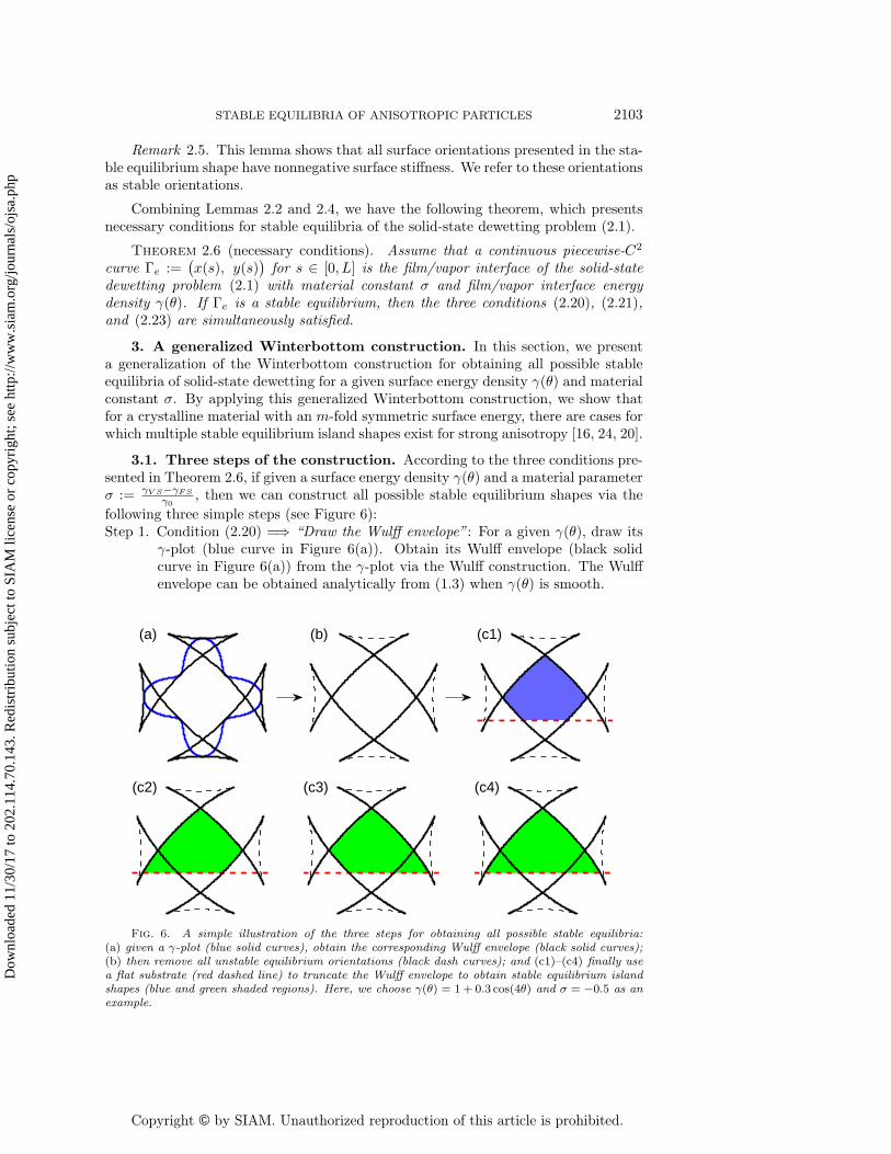
3. A generalized Winterbottom construction. In this section, we presenta generalization of the Winterbottom construction for obtaining all possible stableequilibria of solid-state dewetting for a given surface energy density γ(θ) and materialconstant σ. By applying this generalized Winterbottom construction, we show thatfor a crystalline material with an m-fold symmetric surface energy, there are cases forwhich multiple stable equilibrium island shapes exist for strong anisotropy [16, 24, 20].

3.1. Three steps of the construction. According to the three conditions pre-sented in Theorem 2.6, if given a surface energy density γ(θ) and a material parameterσ := γV S−γFS

γ0, then we can construct all possible stable equilibrium shapes via the

following three simple steps (see Figure 6):Step 1. Condition (2.20) =⇒ “Draw the Wulff envelope”: For a given γ(θ), draw its

γ-plot (blue curve in Figure 6(a)). Obtain its Wulff envelope (black solidcurve in Figure 6(a)) from the γ-plot via the Wulff construction. The Wulffenvelope can be obtained analytically from (1.3) when γ(θ) is smooth.

(a) (b) (c1)

(c2) (c3) (c4)

Fig. 6. A simple illustration of the three steps for obtaining all possible stable equilibria:(a) given a γ-plot (blue solid curves), obtain the corresponding Wulff envelope (black solid curves);(b) then remove all unstable equilibrium orientations (black dash curves); and (c1)–(c4) finally usea flat substrate (red dashed line) to truncate the Wulff envelope to obtain stable equilibrium islandshapes (blue and green shaded regions). Here, we choose γ(θ) = 1 + 0.3 cos(4θ) and σ = −0.5 as anexample.

Dow

nloa

ded

11/3

0/17

to 2

02.1

14.7

0.14

3. R

edis

trib

utio

n su

bjec

t to

SIA

M li

cens

e or

cop

yrig

ht; s

ee h

ttp://

ww

w.s

iam

.org

/jour

nals

/ojs

a.ph

p



Step 2. Condition (2.23) =⇒ “Remove all unstable orientations”: Remove all ori-entations from the Wulff envelope (obtained in Step 1) for which the sur-face stiffness is negative (black dashed curves in Figure 6(b)). As shown inFigure 6(b), only parts of the Wulff envelope “ears” are unstable.

Step 3. Condition (2.21) =⇒ “Truncate the Wulff envelope”: Add a flat substratey = σ (red dashed line in Figures 6(c1)–(c4)) and discard the sections ofthe remaining Wulff envelope (obtained in Step 2). The origin of the x-ycoordinates lies at the center of the Wulff envelope (i.e., the Wulff pointshown in Figure 2(a)). Stable equilibria are enclosed by the Wulff envelopeand the substrate line (blue shaded region in Figure 6(c1) and green shadedregions in Figures 6(c2)–(c4)).

In general, when the surface energy is isotropic or weakly anisotropic (i.e., theWulff envelope has no “ears”), this procedure can produce at most one stable equilib-rium. This is the most widely discussed application of the Winterbottom construction.However, when the surface energy is strongly anisotropic, this procedure may producemultiple stable equilibria, depending on the position of the flat substrate line (i.e., thematerial constant σ). For example, if we choose σ = 0.25, this will produce only onestable equilibrium; on the contrary, if we choose σ = −0.5 (shown in Figure 6), it willproduce four stable equilibria, including two symmetric shapes ((c1) and (c4)) andtwo asymmetric shapes ((c2) and (c3)). In the following discussion, we focus largelyon cases of strong anisotropy.

3.2. Stable equilibria in strongly anisotropic cases. Here we discuss moredetails regarding stable equilibrium shapes found by application of the generalizedWinterbottom construction for solid thin films with m-fold (m = 2, 3, 4, 6) smooth,symmetric film/vapor interface energy densities, which are widely discussed in thematerials science literature. We write this surface energy density in the form

γ(θ) = 1 + β cos[m(θ + φ)

], θ ∈ [−π, π],(3.1)

where φ ∈ [0, π] represents a phase shift angle describing the rotation of the islandcrystal structure with respect to the substrate plane, and β (≥ 0) controls the degreeof the anisotropy. For this surface energy, when β = 0 the system is isotropic; when0 < β < 1

m2−1 it is weakly anisotropic; otherwise, it is strongly anisotropic.We now focus on four strongly anisotropic cases where the substrate line intersects

with part of the Wulff envelope “ears”; these are cases not addressed in the classicalWinterbottom construction [19, 43].

Case 1 (unique stable equilibrium with an inverted shape). When the flat substrateline intersects with the top “ear” of the Wulff envelope (see Figures 7(a)–(d)), thestable equilibrium can be obtained by “flipping over” the truncated part of the Wulffenvelope, as shown in Figures 7(c) and (d). Two different equilibrium island shapesare seen—the first between the substrate line (red) and dashed black line (shadedin green in Figure 7(c)) and the second between the substrate line and the solidblack line (shaded in blue in Figure 7(d)). The first one (in green) is unstable, whilethe second (in blue) is stable. Interestingly, the stable case shown by Figure 7(d)has concave rather than convex surfaces. This is quite different from the classicalWinterbottom/Wulff constructions where the island/particle shape is always convex.The convexity of Wulff shapes has been rigorously proven by [31]. In this example, theanisotropic Young equation (2.21) has two different roots (i.e., θa = 0.3425, 0.6863)in [0, π], but only the root 0.6863 corresponds to the left contact angle of the stableequilibrium shape shown by Figure 7(d).

Dow

nloa

ded

11/3

0/17

to 2

02.1

14.7

0.14

3. R

edis

trib

utio

n su

bjec

t to

SIA

M li

cens

e or

cop

yrig

ht; s

ee h

ttp://

ww

w.s

iam

.org

/jour

nals

/ojs

a.ph

p



(e)(a) Zoom in

σ = −1.6

σ = 1.75

(c)

(b)

(d)

Fig. 7. Generalized Winterbottom constructions for m = 2, β = 0.7, φ = 0 with (b)–(d) σ =1.75 and (e) σ = −1.6, where (a) the solid and dashed black curves show the stable equilibriumand unstable equilibrium sections of the Wulff envelope (with its “ears”), and the red dashed linescorrespond to the substrate for two different values of σ; (b) an enlarged section of the upper portionof the plot in (a) around the substrate line σ = 1.75; (c) an inverted form of (b)—the green shadingrepresents the unstable equilibrium island shape; (d) an inverted form of (b)—the blue shadingrepresents the stable equilibrium island shape; (e) the truncated Wulff envelope shape when σ =−1.6—in this case, the two contact points meet each other, and a complete dewetting will occur(i.e., the island becomes a free particle not attached to the substrate).

Case 2 (a self-intersection curve with complete dewetting). When σ = −1.6, theflat substrate line intersects the bottom “ear” (see Figures 7(a) and (e)), and thetruncated Wulff envelope shape is a self-intersection curve, shown by Figure 7(e). Inthis case, the two contact points meet each other, and complete dewetting occurs—this implies that the island becomes an isolate particle, detached from the substrate.Note here that in this example, the anisotropic Young equation (2.21) has only oneroot (i.e., θa = 2.2497), and it is less than π.

Case 3 (unique stable equilibrium). When the flat substrate line intersects themiddle “ears” of the Wulff envelope above the center, only one stable equilibriumshape exists and that is the one represented by the classical Winterbottom construc-tion. In this example (i.e., γ(θ) = 1 + 0.3 cos(4θ) and σ = 0.25), the anisotropicYoung equation (2.21) has three different roots (θa = 0.8471, 1.6436, 2.1649) in[0, π], but only the root θa = 0.8471 corresponds to the left contact angle of the stableequilibrium shape.

Case 4 (multiple stable equilibria). In this case, the substrate line intersectsthe middle “ears” below the center. As shown in Figure 8, it admits three solu-tions to the anisotropic Young equation (2.21). For the case shown in Figure 8(a)(m = 4, β = 0.3, φ = 0, σ = −0.5, for which stable equilibrium shapes have beenclearly shown by Figure 6), the three solutions for the left contact angle in [0, π] areθa = 1.0563, 1.4146, 2.3575, two of which are stable. This yields the four stableequilibrium shapes—two symmetric (blue shaded region and striped region in Fig-ure 8(a)) and two asymmetric stable equilibrium shapes (blue shaded region plus thestriped regions to the left or right of it in Figure 8(a)). Similarly, for the case shown inFigure 8(b) (m = 4, β = 0.4, φ = 0, σ = −

√3/2), there are three solutions in [0, π] for

the left contact angle θa = 1.0672, 1.3723, 2.4520, two of which are stable. However,this yields one symmetric (striped region in Figure 8(b)) and two asymmetric stableequilibrium shapes (blue shaded region plus the striped regions on the left or rightof the center of the blue region in Figure 8(b)), together with a completely dewettedparticle (the blue region detached from the substrate in Figure 8(b)).

Dow

nloa

ded

11/3

0/17

to 2

02.1

14.7

0.14

3. R

edis

trib

utio

n su

bjec

t to

SIA

M li

cens

e or

cop

yrig

ht; s

ee h

ttp://

ww

w.s

iam

.org

/jour

nals

/ojs

a.ph

p



(a) (b)

Fig. 8. Two different examples for Case 4, where the generalized Winterbottom constructionsare given for (a) m = 4, β = 0.3, φ = 0, σ = −0.5; (b) m = 4, β = 0.4, φ = 0, σ = −

√3/2.

The four cases discussed here clearly show that the anisotropic Young equation(2.21) may have multiple roots in [0, π] (corresponding to static values of the left con-tact angles), but it is not necessarily the case that all of these are stable; i.e., thereare stable and unstable anisotropic Young angles. More precisely, “stable anisotropicYoung angles” refer here to all roots to (2.21) for which (2.23) is satisfied, i.e., equi-librium contact angles which may occur for stable orientations. For the m-fold crys-talline surface energy (3.1) with φ = 0, we find that a stable anisotropic Young angleuniquely determines a symmetric stable equilibrium shape. Hence, the number of sta-ble anisotropic Young angles reflects the number of stable equilibrium island shapes.For a fixed φ, we can examine how the number of anisotropic Young angles (i.e., theroots of the anisotropic Young equation (2.21) in [0, π]) and the number of those thatare stable vary with the magnitude of the anisotropy β and the material constantσ. We show these numbers of anisotropic Young angles as a function of β and σfor m-fold symmetric crystals (m = 2, 3, 4, 6) in Figure 9 (for φ = 0). As shown inFigure 9, when m increases, the maximum number of stable anisotropic Young anglesalso increases, and this means that more stable equilibrium shapes may appear (notethat we only show data for 0 ≤ β < 1 since outside this range, the surface energydensity γ(θ) may be nonpositive).

4. Dynamical evolution via surface diffusion. In the previous section, weshowed that when the surface energy is strongly anisotropic, multiple stable equilib-rium island shapes (and contact angles) are possible. Which equilibrium shape ap-pears may depend on how the system evolves, i.e., it may be possible for the systemto be trapped in a metastable equilibrium. In order to investigate this question, wepropose the dynamical evolution sharp-interface model via surface diffusion-controlledshape evolution for simulating solid-state dewetting and finding numerical stationary(or equilibrium) shapes. In the following section, we present numerical results forthis model, evolving the structure until the shape becomes stationary, and comparethe resulting morphologies with those predicted in the previous section. We previ-ously outline this approach in [41, 16] and describe it here for (i) the isotropic/weaklyanisotropic, (ii) the strongly anisotropic, and (iii) the nonsmooth and/or “cusped”surface energy cases.

4.1. Isotropic/weakly anisotropic case. In this case, γ(θ) ∈ C2[−π, π] andγ(θ) := γ(θ) + γ ′′(θ) > 0 ∀ θ ∈ [−π, π], where the first variation was shown in (2.13).A sharp-interface model for the 2D solid-state dewetting of an island/film on a flat

Dow

nloa

ded

11/3

0/17

to 2

02.1

14.7

0.14

3. R

edis

trib

utio

n su

bjec

t to

SIA

M li

cens

e or

cop

yrig

ht; s

ee h

ttp://

ww

w.s

iam

.org

/jour

nals

/ojs

a.ph

p



10 2 3 4 5 6

−3 −2 −1 0 1 2 30

0.5

1

0 0

1 1

1

σ

β

(a)

1

3

−3 −2 −1 0 1 2 30

0.5

1

0 0

11

1

21

σ

β

(b)

1

8

−3 −2 −1 0 1 2 30

0.5

1

0 0

1

1 1

112

2 1

11

σ

β

(c)

1

15

−3 −2 −1 0 1 2 30

0.5

1

1 1

12

12 2

13

13

12 211 11

σ

β

1

35

(d)

0 0

Fig. 9. Phase diagrams of the number of anisotropic Young angles (roots of the anisotropicYoung equation (2.21) in [0, π]) as a function of β and σ for (a) m = 2, (b) m = 3, (c) m = 4,and (d) m = 6 (under the fixed φ = 0). The colors indicate the total number of anisotropic Youngangles—see the color bar at the top. The Arabic numerals in each of the plots indicate the numberof stable anisotropic Young angles. Of course, the number of stable anisotropic Young angles is lessthan or equal to the number of roots of (2.21).

Dow

nloa

ded

11/3

0/17

to 2

02.1

14.7

0.14

3. R

edis

trib

utio

n su

bjec

t to

SIA

M li

cens

e or

cop

yrig

ht; s

ee h

ttp://

ww

w.s

iam

.org

/jour

nals

/ojs

a.ph

p



rigid substrate via surface diffusion was proposed in [41, 2]. In dimensionless form,the model may be written as

Xt = µss n, 0 < s < L(t), t > 0,(4.1)µ =

[γ(θ) + γ ′′(θ)

]κ, κ = −yssxs + xssys,(4.2)

where Γ := Γ(t) = X(s, t) = (x(s, t), y(s, t)) represents the moving film/vapor inter-face, s is the arc length or distance along the interface, t is time, n = (−ys, xs) isthe interface outer unit normal direction, µ := µ(s, t) is the chemical potential, andL := L(t) represents the total length of the moving film/vapor interface. The initialcondition is

X(s, 0) = (x(s, 0), y(s, 0)) = X0(s) = (x0(s), y0(s)), 0 ≤ s ≤ L0 := L(0),(4.3)

and the boundary conditions are as follows [41]:(i) contact point condition,

y(0, t) = 0, y(L, t) = 0, t ≥ 0;(4.4)

(ii) relaxed contact angle condition,

dxlcdt

= η f(θld;σ),dxrcdt

= −η f(θrd;σ), t ≥ 0,(4.5)

where θld := θld(t) and θrd := θrd(t) are the (dynamic) contact angles at the leftand right contact points, respectively, 0 < η < ∞ denotes the contact linemobility, and f(θ;σ) is defined as in (2.14);

(iii) zero-mass flux condition,

µs(0, t) = 0, µs(L, t) = 0, t ≥ 0.(4.6)

Condition (4.4) implies that the two contact points must move along the flatsubstrate, condition (4.5) is the energy dissipation relation for the moving contactpoints [41], and condition (4.6) ensures that the total area/mass of the thin film isconserved (no mass flux at the moving contact points). The total area/mass of theisland A(t) and the total interfacial energy W (t) are defined as

A(t) =∫ L(t)

0y(s, t)xs(s, t) ds, W (t) =

∫ L(t)

0γ(θ(s, t)) ds− σ

[xrc(t)− xlc(t)

].

(4.7)

Proposition 4.1. For the sharp-interface model governing by (4.1)–(4.2) togetherwith boundary conditions (4.4)–(4.6) and the initial condition (4.3), the total area/massis conserved and the total interfacial energy decreases during the evolution in theisotropic or weakly anisotropic case:

A(t) ≡ A(0) =∫ L(0)

0y(s, 0)xs(s, 0) ds, t ≥ 0,(4.8)

W (t) ≤W (t1) ≤W (0) =∫ L(0)

0γ(θ(s, 0)) ds− σ

[xrc(0)− xlc(0)

], t ≥ t1 ≥ 0.(4.9)

Dow

nloa

ded

11/3

0/17

to 2

02.1

14.7

0.14

3. R

edis

trib

utio

n su

bjec

t to

SIA

M li

cens

e or

cop

yrig

ht; s

ee h

ttp://

ww

w.s

iam

.org

/jour

nals

/ojs

a.ph

p



Proof. We first introduce a new time-independent variable p ∈ [0, 1] and re-parameterize the moving film/vapor interface such that p = 0 and p = 1 represent theleft and right contact points, respectively. Then the arc length s is a function of p andt and we denote sp = ∂s

∂p . The area/mass of the thin film in (4.8) can be rewritten as

A(t) =∫ 1

0yxp dp.(4.10)

By differentiating (4.10) with respect to t and integrating by parts, we obtain

A(t) =∫ 1

0(ytxp + yxpt) dp =

∫ 1

0(ytxp − ypxt) dp+ yxt|p=1

p=0

=∫ 1

0(xt, yt) · (−yp, xp) dp =

∫ L(t)

0Xt · n ds

=∫ L(t)

0µss ds = µs

(L(t), t

)− µs

(0, t)

= 0,(4.11)

which immediately implies the total area/mass is conserved.The total free energy in (4.9) can be rewritten as

W (t) =∫ 1

0γ(θ)sp dp− σ

[xrc(t)− xlc(t)

].(4.12)

Notice that the following equations hold:

np = κspτ , τ p = −κspn, θp = −κsp, spt = Xpt · τ , θtsp = Xpt · n.(4.13)

Differentiating (4.12) with respect to t and integrating by parts, making use of theabove identities (4.13) and (4.1)–(4.6), we obtain

W (t) =∫ 1

0(γ ′(θ)θtsp + γ(θ)spt) dp− σ

(dxrcdt− dxlc

dt

)=∫ 1

0Xpt ·

(γ ′(θ) n + γ(θ) τ

)dp− σ

(dxrcdt− dxlc

dt

)= −

∫ 1

0Xt ·

((γ ′′(θ)θpn + γ ′(θ)κspτ

)+(γ ′(θ)θpτ − γ(θ)κspn

))dp

+[Xt ·

(γ ′(θ) n + γ(θ) τ

)]p=1p=0 − σ

(dxrcdt− dxlc

dt

)=∫ L(t)

0κ(γ(θ) + γ ′′(θ)

)Xt · n ds+ f(θrd;σ)

dxrcdt− f(θld;σ)

dxlcdt

(4.14)

=∫ L(t)

0µµss ds−

1η

[(dxrcdt

)2

+(dxlcdt

)2]

= µµs|s=L(t)s=0 −

∫ L(t)

0µ2s ds−

1η

[(dxrcdt

)2

+(dxlcdt

)2]

= −∫ L(t)

0µ2s ds−

1η

[(dxrcdt

)2

+(dxlcdt

)2]≤ 0, t ≥ 0,(4.15)

which demonstrates that the total free energy is dissipative during the evolution.

Dow

nloa

ded

11/3

0/17

to 2

02.1

14.7

0.14

3. R

edis

trib

utio

n su

bjec

t to

SIA

M li

cens

e or

cop

yrig

ht; s

ee h

ttp://

ww

w.s

iam

.org

/jour

nals

/ojs

a.ph

p



4.2. Strongly anisotropic case. In this case, γ(θ) ∈ C2[−π, π] and the surfacestiffness γ(θ) := γ(θ) + γ ′′(θ) changes sign for some θ ∈ [−π, π], and the governingequations (4.1)–(4.2) become ill-posed. These governing equations can be regularizedby adding regularization terms such that the regularized sharp-interface model iswell-posed. In practice, this is often done by regularizing the total interfacial energyW (Γ) in (2.1) by adding the well-known Willmore energy, i.e., Wwm = 1

2

∫Γ κ

2 dΓ[12, 40, 16, 2], such that the regularized total interfacial energy becomes

W εreg(Γ) = W (Γ) + ε2Wwm(Γ) =

∫Γ

[γ(θ) +

ε2

2κ2]dΓ− σ(xrc − xlc),(4.16)

where 0 < ε 1 is a small regularization parameter.Similar to the calculation of the first variation of W (Γ) in (2.1) to obtain (2.13),

we obtain the first variation of the regularized total interfacial energy W εreg(Γ) as

(details omitted here for brevity) [16]

δW εreg(Γ;ϕ,ψ) =

∫ L

0µε(s)ϕ(s) ds+ fε(θrd;σ)u(L)− fε(θld;σ)u(0)

− (κϕs)|L0 +(

12κ2ψ

)∣∣∣∣L0,(4.17)

where the function fε(θ;σ) is defined as

fε(θ;σ) := γ(θ) cos θ − γ ′(θ) sin θ − σ − ε2κs(θ) sin θ,(4.18)

and µε := µε(s) represents the dimensionless (regularized) chemical potential of thesystem, i.e.,

µε(s) := γ(θ)κ− ε2(κ3

2+ κss

), γ(θ) = γ(θ) + γ′′(θ), κ = −yssxs + xssys.(4.19)

For ε → 0, if κs(θ) = o(1/ε2) at contact points, then fε(θ;σ) → f(θ;σ), which isdefined in (2.14).

A sharp-interface model for the solid-state dewetting of a 2D island/film withstrongly anisotropic surface energy γ(θ) on a flat rigid substrate can be written as (indimensionless form) [16, 2]

Xt =(µε)ss

n, 0 < s < L(t), t > 0.(4.20)

The initial condition is (4.3), the first boundary condition is (i) the contact pointcondition (4.4), and the other boundary conditions can be written as follows:

(ii′) relaxed contact angle condition,

dxlcdt

= η fε(θld;σ),dxrcdt

= −η fε(θrd;σ), t ≥ 0,(4.21)

(iii′) zero-mass flux condition,(µε)s(0, t) = 0,

(µε)s(L, t) = 0, t ≥ 0,(4.22)

Dow

nloa

ded

11/3

0/17

to 2

02.1

14.7

0.14

3. R

edis

trib

utio

n su

bjec

t to

SIA

M li

cens

e or

cop

yrig

ht; s

ee h

ttp://

ww

w.s

iam

.org

/jour

nals

/ojs

a.ph

p



(iv) zero-curvature condition,

κ(0, t) = 0, κ(L, t) = 0, t ≥ 0.(4.23)

Compared to the isotropic/weakly anisotropic case, the contact point condition(4.4) is the same and the boundary conditions (4.21)–(4.22) are similar. However,the additional boundary condition (4.23) is obtained from the first variation of thefree energy (4.17) such that the system is self-closed (the dynamical evolution PDEsbecome sixth-order while they are fourth-order for the isotropic/weakly anisotropiccase) and the total (regularized) free energy is dissipative during the evolution. Infact, this zero-curvature boundary condition (4.23) may be interpreted as the shapetends to be faceted near the two contact points when the surface energy anisotropyis strong.

As a function of time, the total (regularized) interfacial energy is defined as

W εreg(t) :=

∫ L(t)

0

[γ(θ) +

ε2

2κ2]ds− σ

[xrc(t)− xlc(t)

].(4.24)

Proposition 4.2. For the sharp-interface model governed by (4.20) and (4.19),together with boundary conditions (4.4) and (4.21)–(4.23) and initial condition (4.3),the total area/mass is conserved (i.e., (4.8) is valid), and the total (regularized) in-terfacial energy decreases during the evolution, i.e.,

W εreg(t) ≤W ε

reg(t1) ≤W εreg(0), t ≥ t1 ≥ 0.(4.25)

Proof. The proof that the total area/mass is conserved is similar to the proof ofProposition 4.1 and is omitted here for brevity. In order to prove that the energyis always decreasing during the evolution, the Willmore regularization energy can berewritten as

Wwm(t) =12

∫ 1

0κ2sp dp.(4.26)

Differentiating (4.26) with respect to t, making use of (4.13) and the identity κtsp =−θpt − κspt, applying (4.23), and integrating by parts, we obtain

Wwm(t) =12

∫ 1

0

(2κκtsp + κ2spt

)dp =

∫ 1

0

(−κθpt − κ2spt +

12κ2spt

)dp

=∫ 1

0

(−κθpt −

12κ2spt

)dp =

∫ 1

0

(κsspθt −

12κ2spt

)dp

=∫ 1

0Xpt ·

(κsn−

12κ2τ

)dp

= −∫ 1

0Xt ·

(κssspn + κsnp − κκsspτ −

12κ2τ p

)dp+

(κsXt · n

)p=1p=0

= −∫ L(t)

0

(κss +

12κ3)

Xt · n ds− (κs sin θ)θ=θrddxrcdt

+ (κs sin θ)θ=θlddxlcdt

.(4.27)

Dow

nloa

ded

11/3

0/17

to 2

02.1

14.7

0.14

3. R

edis

trib

utio

n su

bjec

t to

SIA

M li

cens

e or

cop

yrig

ht; s

ee h

ttp://

ww

w.s

iam

.org

/jour

nals

/ojs

a.ph

p



Combining (4.27) and (4.14), applying (4.21)–(4.22) and integrating by parts, we have

W εreg(t) =

∫ L(t)

0

(γ(θ)κ− ε2

(κss +

12κ3))

Xt · n ds+ fε(θrd;σ)dxrcdt− fε(θld;σ)

dxlcdt

=∫ L(t)

0µε(µε)ss ds−

1η

[(dxrcdt

)2

+(dxlcdt

)2]

= −∫ L(t)

0(µε)2

s ds−1η

[(dxrcdt

)2

+(dxlcdt

)2]≤ 0, t ≥ 0,(4.28)

which immediately implies (4.25).

4.3. Nonsmooth and/or “cusped” cases. In this case, γ(θ) ∈ C0[−π, π]but γ(θ) /∈ C2[−π, π]. In most anisotropic solid-state dewetting analyses, it is as-sumed that the surface energy γ(θ) is piecewise smooth and is only nonsmooth and/or“cusped” at a finite set of points. A typical example can be given as [2, 32]

γ(θ) = 1 + β cos[m(θ + φ)] +n∑i=1

| sin(θ − αi)|, θ ∈ [−π, π],(4.29)

where n is a positive integer, β ≥ 0 is a constant, m is a positive integer, and φ ∈ [0, π]and αi ∈ [0, π] for i = 1, 2, . . . , n are constants.

In this situation, we can first smooth the surface energy γ(θ) by a C2-smoothfunction γδ(θ) with a smoothing parameter 0 < δ 1 such that γδ(θ) convergesuniformly to γ(θ) for θ ∈ [−π, π] when δ → 0+. For the above example, we use

γδ(θ) = 1 + β cos[m(θ + φ)] +n∑i=1

√δ2 + (1− δ2) sin2(θ − αi), θ ∈ [−π, π].(4.30)

If the smoothed surface energy γδ(θ) is weakly anisotropic, γδ(θ) + γ′′δ (θ) > 0∀ θ ∈ [−π, π]), we can apply the sharp-interface model presented in section 4.1 by re-placing γ(θ) with γδ(θ). On the other hand, if the smoothed surface energy is stronglyanisotropic, γδ(θ) + γ′′δ (θ) < 0 for some θ ∈ [−π, π], we must use the (regularized)sharp-interface model with a regularization parameter 0 < ε 1 (see section 4.2) byreplacing γ(θ) with γδ(θ).

5. Numerical validation. In this section, we present six examples to vali-date the proposed generalized Winterbottom construction by numerically solving theproposed dynamical evolution equations for the mass transport via surface diffusioncoupled with contact line migration. These examples will also show that metastable is-land shapes are dynamically accessible. The first four examples correspond to the fourcases discussed in section 3 and the other two are for an m-fold smooth surface energyγ(θ) with a nonzero phase angle φ and nonsmooth surface energy γ(θ) with “cusps”.For the weakly anisotropic case, (4.1)–(4.2) coupled with boundary conditions (4.4)–(4.6) are numerically solved; for the strongly anisotropic case, (4.19)–(4.20) coupledwith boundary conditions (4.4) and (4.21)–(4.23) are numerically solved. We employa semi-implicit parametric finite element method recently proposed by [2] for solvingthe above two cases. We note that for these two cases, we have rigorously proved that

Dow

nloa

ded

11/3

0/17

to 2

02.1

14.7

0.14

3. R

edis

trib

utio

n su

bjec

t to

SIA

M li

cens

e or

cop

yrig

ht; s

ee h

ttp://

ww

w.s

iam

.org

/jour

nals

/ojs

a.ph

p



−1 0 10

1

(a)

x

y

Initial state Wulff envelope Numerical equilibrium

−1 0 10

1

(b)

x

y

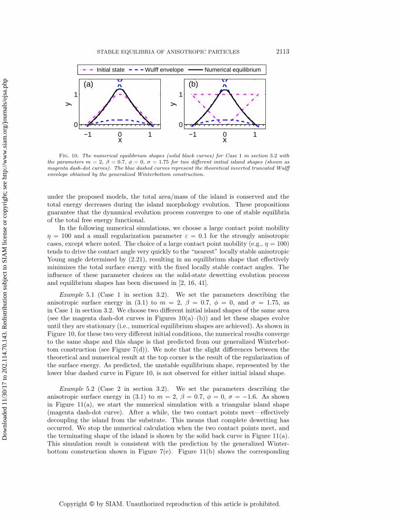
Fig. 10. The numerical equilibrium shapes (solid black curves) for Case 1 in section 3.2 withthe parameters m = 2, β = 0.7, φ = 0, σ = 1.75 for two different initial island shapes (shown asmagenta dash-dot curves). The blue dashed curves represent the theoretical inverted truncated Wulffenvelope obtained by the generalized Winterbottom construction.

under the proposed models, the total area/mass of the island is conserved and thetotal energy decreases during the island morphology evolution. These propositionsguarantee that the dynamical evolution process converges to one of stable equilibriaof the total free energy functional.

In the following numerical simulations, we choose a large contact point mobilityη = 100 and a small regularization parameter ε = 0.1 for the strongly anisotropiccases, except where noted. The choice of a large contact point mobility (e.g., η = 100)tends to drive the contact angle very quickly to the “nearest” locally stable anisotropicYoung angle determined by (2.21), resulting in an equilibrium shape that effectivelyminimizes the total surface energy with the fixed locally stable contact angles. Theinfluence of these parameter choices on the solid-state dewetting evolution processand equilibrium shapes has been discussed in [2, 16, 41].

Example 5.1 (Case 1 in section 3.2). We set the parameters describing theanisotropic surface energy in (3.1) to m = 2, β = 0.7, φ = 0, and σ = 1.75, asin Case 1 in section 3.2. We choose two different initial island shapes of the same area(see the magenta dash-dot curves in Figures 10(a)–(b)) and let these shapes evolveuntil they are stationary (i.e., numerical equilibrium shapes are achieved). As shown inFigure 10, for these two very different initial conditions, the numerical results convergeto the same shape and this shape is that predicted from our generalized Winterbot-tom construction (see Figure 7(d)). We note that the slight differences between thetheoretical and numerical result at the top corner is the result of the regularization ofthe surface energy. As predicted, the unstable equilibrium shape, represented by thelower blue dashed curve in Figure 10, is not observed for either initial island shape.

Example 5.2 (Case 2 in section 3.2). We set the parameters describing theanisotropic surface energy in (3.1) to m = 2, β = 0.7, φ = 0, σ = −1.6. As shownin Figure 11(a), we start the numerical simulation with a triangular island shape(magenta dash-dot curve). After a while, the two contact points meet—effectivelydecoupling the island from the substrate. This means that complete dewetting hasoccurred. We stop the numerical calculation when the two contact points meet, andthe terminating shape of the island is shown by the solid back curve in Figure 11(a).This simulation result is consistent with the prediction by the generalized Winter-bottom construction shown in Figure 7(e). Figure 11(b) shows the corresponding

Dow

nloa

ded

11/3

0/17

to 2

02.1

14.7

0.14

3. R

edis

trib

utio

n su

bjec

t to

SIA

M li

cens

e or

cop

yrig

ht; s

ee h

ttp://

ww

w.s

iam

.org

/jour

nals

/ojs

a.ph

p



−1 0 10

1

2 (a)

x

y

0 0.1 0.2

1

2

(b)

t

θ dlFig. 11. Simulation results for Case 2 in section 3.2 with parameters m = 2, β = 0.7, φ = 0,

σ = −1.6: (a) the final state of the numerical evolution which was stopped when the two contactpoints meet; (b) the temporal evolution of the left dynamical contact angle (blue curve) as it convergesto the theoretical anisotropic Young angle θa = 2.2497 (red dashed line).

−1 0 10

1

(a)

x

y


−1 0 10

1

(b)

x

y

Fig. 12. The numerical equilibrium shapes (solid black curves) for Case 3 in section 3.2 withthe parameters: m = 4, β = 0.3, φ = 0, σ = 0.25 for two different initial island shapes (magentadash-dot curves). The blue dashed curve represents the theoretical truncated Wulff envelope obtainedfrom the generalized Winterbottom construction, Figure 6(c).

temporal evolution of the left dynamic contact angle. As is clearly seen in this fig-ure, the numerical left dynamic contact angle converges to the theoretical anisotropicYoung angle θa = 2.2497.

Example 5.3 (Case 3 in section 3.2). We choose the same set of parametersm = 4, β = 0.3, φ = 0, σ = 0.25 as the Case 3 in section 3.2. As shown in Figure 12,for both of the two very different initial shapes, the system evolves to the same final,stationary shape. This shape is in good agreement with the stable equilibrium shapeFigure 6(c) predicted by the generalized Winterbottom construction.

Example 5.4 (Case 4 in section 3.2). For Case 4, we choose the same set of pa-rameters m = 4, β = 0.4, φ = 0, σ = −

√3/2 as in Figure 8(b) in section 3.2. As

predicted by the generalized Winterbottom construction, three different stable equi-librium shapes and complete dewetting are the solutions. More precisely, these stableequilibria include a symmetric stable equilibrium island shape shown in Figure 13(a),two asymmetric stable equilibrium shapes shown in Figure 13(b) (its mirror is also asolution, not shown here), and complete dewetting shown in Figure 13(c) (its numer-ical simulation was stopped when the two contact points met). All of these shapescorrespond to the theoretical predictions obtained from the generalized Winterbottom

Dow

nloa

ded

11/3

0/17

to 2

02.1

14.7

0.14

3. R

edis

trib

utio

n su

bjec

t to

SIA

M li

cens

e or

cop

yrig

ht; s

ee h

ttp://

ww

w.s

iam

.org

/jour

nals

/ojs

a.ph

p



−2 −1 0 1 20

1

2(a)

x

y

−1 0 1 20

1

2(b)

xy


−2 −1 0 1 20

1

2 (c)

x

y

Initial stateTerminating state

Fig. 13. Multiple equilibria (black solid curves) are found for Case 4 with the parameters m = 4,β = 0.4, φ = 0, σ = −

√3/2 for three different initial island shapes (magenta dash-dot curves). The

energies of these three states decrease from (a) to (c), indicating that the classical Winterbottomconstruction prediction yields the globally minimum energy island shape (note that the shape in (b)has a mirror symmetric counterpart, not shown here).

−1 0 1

−1

0

1φ

(a)

−4 −2 0 2 40

2

(b)

−4 −2 0 2 40

2

(c)

Fig. 14. (a) Illustration of the generalized Winterbottom construction for an m-fold smoothsurface energy described by the parameters m = 4, β = 0.3, and σ = 0.2 for the case in whichthe crystal structure of the island is rotated with respect to the substrate by φ = π/6. The stableequilibrium shapes for these parameters are shown by the horizontal stripes and blue-shaded regions.(b), (c) Numerical equilibrium states (black solid curves) for solid-state dewetting starting withdifferent initial shapes (magenta dash-dot curves) for the same set of parameters.

construction. By comparing the numerical equilibrium shapes with the generalizedWinterbottom predictions, we find that they are in good accordance with each other.These results demonstrate that not only the global equilibrium island shape but alsoall of the metastable island shapes are dynamically attainable. This shows that it isnecessary to consider the generalization of the Winterbottom construction and notjust the classical Winterbottom construction in understanding experimentally observ-able island morphologies.

Example 5.5 (m-fold smooth surface energy with a nonzero phase angle φ). Inorder to demonstrate the generality of our proposed generalized Winterbottom con-struction, we also present an example of an m-fold symmetry crystalline island withm = 4, β = 0.3, and σ = 0.2, where the crystal lattice of the island is rotated byφ = π/6 (relative to the substrate surface normal). As seen in Figure 14(a), two differ-ent stable equilibria are found from the generalized Winterbottom construction (blue

Dow

nloa

ded

11/3

0/17

to 2

02.1

14.7

0.14

3. R

edis

trib

utio

n su

bjec

t to

SIA

M li

cens

e or

cop

yrig

ht; s

ee h

ttp://

ww

w.s

iam

.org

/jour

nals

/ojs

a.ph

p



−2 −1 0 1 2

−1

0

1 (a)

−1 0 10

1 (b)

−1 0 10

1 (d)

−1 0 10

1 (c)

Fig. 15. (a) Illustration of the generalized Winterbottom construction for a nonsmooth surfaceenergy with “cusps” as per (4.29), where the parameters were set to m = 4, β = 0.25, φ = 0, n =1, α1 = 0, σ = −0.3. The blue shaded and horizontal striped regions indicate different stable equilib-rium shapes. (b)–(d) Numerical stable solutions (black solid curves) found from evolving the islandshapes from different initial shapes (magenta dash-dot curves) using the smoothed surface energy,defined in (4.30) with ε = δ = 0.05 (note that the shape in (c) has a mirror symmetric counterpart,not shown here).

shaded and horizontally striped regions). We show the numerically stable solutions inFigures 14(b)–(c) (solid black curves) obtained for two different initial island shapes(magenta dash-dot curves). We observe that these two different initial conditionsconverge to two different stationary states—both of the shapes (one correspondingto the global equilibrium and one metastable) are predicted from the generalizedWinterbottom construction.

Example 5.6 (nonsmooth surface energy with “cusps”). For this example, weperform numerical calculations for the nonsmooth (cusped) surface energy densityγ(θ) in (4.29) for the parameters m = 4, β = 0.25, φ = 0, n = 1, and α1 = 0.Figure 15(a) depicts the generalized Winterbottom construction for this nonsmoothsurface energy density and σ = −0.3. Applying the generalized Winterbottom con-struction to this case, we find four distinct stable equilibria (the asymmetric one hasa mirror symmetry, not shown here). Figures 15(b)–(d) show the numerical equilib-rium states obtained (black solid curves) starting from three different initial shapes(magenta dash-dot curves) along with the Winterbottom predictions for the same setof parameters. The numerical calculations were performed with δ = 0.05 in (4.30)and ε = 0.05 in (4.20). Again, the agreement between the numerical results and ourtheoretical predictions is excellent. The energies for these equilibrium shapes increasefrom (b) to (d)—the symmetric island shape in (b) is the classical Winterbottomprediction corresponding to the global minimum energy shape.

6. Conclusions. We have presented a new approach to predicting stable equilib-rium shapes of 2D crystalline islands on flat substrates. Our theory is a generalizationof the widely used, classical Winterbottom construction [43]. This approach is equallyapplicable to isotropic, weakly anisotropic, strongly anisotropic, and “cusped” crystalsurface energy functions. We predict that, unlike in the classical Winterbottom ap-proach, multiple equilibrium island shapes may be possible. We analyzed these shapesthrough a perturbation analysis, by calculating the first and second variations of thetotal free energy functional with respect to contact positions and island shape. Based

Dow

nloa

ded

11/3

0/17

to 2

02.1

14.7

0.14

3. R

edis

trib

utio

n su

bjec

t to

SIA

M li

cens

e or

cop

yrig

ht; s

ee h

ttp://

ww

w.s

iam

.org

/jour

nals

/ojs

a.ph

p



on this analysis, we obtained the necessary conditions for the equilibria to be stablewith respect to 2D perturbation and exploit this through a generalization of the Win-terbottom construction to identify all possible stable equilibrium shapes. Finally, wedeveloped a dynamical evolution method based upon surface diffusion mass transportto determine if all of the stable equilibrium shapes are dynamically accessible. Ap-plying this approach, we demonstrated that islands with different initial shapes mayevolve into different stationary shapes and show that these dynamically determinedstationary states correspond to those stable, equilibrium shapes predicted by our new,generalized Winterbottom construction.

REFERENCES

[1] L. Armelao, D. Barreca, G. Bottaro, A. Gasparotto, S. Gross, C. Maragno, andE. Tondello, Recent trends on nanocomposites based on Cu, Ag and Au clusters: Acloser look, Coord. Chem. Rev., 250 (2006), pp. 1294–1314.

[2] W. Bao, W. Jiang, Y. Wang, and Q. Zhao, A parametric finite element method for solid-state dewetting problems with anisotropic surface energies, J. Comput. Phys., 330 (2017),pp. 380–400.

[3] P.-G. De Gennes, Wetting: statics and dynamics, Rev. Mod. Phys., 57 (1985), pp. 827–863.[4] K. Deckelnick, G. Dziuk, and C. M. Elliott, Computation of geometric partial differential

equations and mean curvature flow, Acta Numer., 14 (2005), pp. 139–232.[5] E. Dornel, J. Barbe, F. De Crecy, G. Lacolle, and J. Eymery, Surface diffusion dewetting

of thin solid films: Numerical method and application to Si/SiO2, Phys. Rev. B, 73 (2006),p. 115427.

[6] P. Du and H. Wong, A delta-function model for axially symmetric crystals, Scripta Mater.,55 (2006), pp. 1171–1174.

[7] P. Du and H. Wong, An analytic solution for three-dimensional axisymmetric equilibriumcrystal shapes, Scripta Mater., 60 (2009), pp. 631–634.

[8] I. Fonseca and S. Muller, A uniqueness proof for the Wulff theorem, Proc. Roy. Soc. Edin-burgh, 119 (1991), pp. 125–136.

[9] J. W. Gibbs, On the equilibrium of heterogeneous substances, Trans. Connecticut Acad. ArtsSci., 3 (1878), pp. 104–248.

[10] K. Gurski and G. McFadden, The effect of anisotropic surface energy on the Rayleigh insta-bility, Proc. R. Soc. Lond. Ser. A Math. Phys. Eng. Sci., 459 (2003), pp. 2575–2598.

[11] K. Gurski, G. McFadden, and M. J. Miksis, The effect of contact lines on theRayleigh instability with anisotropic surface energy, SIAM J. Appl. Math., 66 (2006),pp. 1163–1187.

[12] M. E. Gurtin and M. E. Jabbour, Interface evolution in three dimensions with curvature-dependent energy and surface diffusion: Interface-controlled evolution, phase transitions,epitaxial growth of elastic films, Arch. Ration. Mech. Anal., 163 (2002), pp. 171–208.

[13] C. Herring, The Physics of Powder Metallurgy, W. E. Kingston, ed., McGraw-Hill, New York,1951.

[14] D. W. Hoffman and J. W. Cahn, A vector thermodynamics for anisotropic surfaces:I. Fundamentals and application to plane surface junctions, Surface Sci., 31 (1972),pp. 368–388.

[15] W. Jiang, W. Bao, C. V. Thompson, and D. J. Srolovitz, Phase field approach for simu-lating solid-state dewetting problems, Acta Mater., 60 (2012), pp. 5578–5592.

[16] W. Jiang, Y. Wang, Q. Zhao, D. J. Srolovitz, and W. Bao, Solid-state dewetting and islandmorphologies in strongly anisotropic materials, Scripta Mater., 115 (2016), pp. 123–127.

[17] E. Jiran and C. Thompson, Capillary instabilities in thin films, J. Electron. Mater., 19 (1990),pp. 1153–1160.

[18] C. Joshi, T. Abinandanan, and A. Choudhury, Phase field modelling of rayleigh instabilitiesin the solid-state, Acta Mater., 109 (2016), pp. 286–291.

[19] R. Kaischew, Equilibrium shape and work of formation of crystalline nuclei on a foreignsubstrate (in Bulgarian), Commun. Bulg. Acad. Sci., 1 (1950), p. 100.

[20] L. Klinger and E. Rabkin, Shape evolution by surface and interface diffusion with rigid bodyrotations, Acta Mater., 59 (2011), pp. 6691–6699.

[21] M. Koiso and B. Palmer, Anisotropic capillary surfaces with wetting energy, Calc. Var. PartialDifferential Equations, 29 (2007), pp. 295–345.

[22] M. D. Korzec, M. Roczen, M. Schade, B. Wagner, and B. Rech, Equilibrium shapes ofpolycrystalline silicon nanodots, J. Appl. Phys., 115 (2014), 074304.

Dow

nloa

ded

11/3

0/17

to 2

02.1

14.7

0.14

3. R

edis

trib

utio

n su

bjec

t to

SIA

M li

cens

e or

cop

yrig

ht; s

ee h

ttp://

ww

w.s

iam

.org

/jour

nals

/ojs

a.ph

p



[23] R. Kotecky and C.-E. Pfister, Equilibrium shapes of crystals attached to walls, J. Stat.Phys., 76 (1994), pp. 419–445.

[24] O. Kovalenko and E. Rabkin, Mechano-stimulated equilibration of gold nanoparticles onsapphire, Scripta Mater., 107 (2015), pp. 149–152.

[25] M. Laue, Nachtrag zu meiner Arbeit: Eine Ausgestaltung der Londonschen Theorie derSupraleitung, Ann. Phys., 435 (1943), pp. 223–224.

[26] F. Leroy, F. Cheynis, Y. Almadori, S. Curiotto, M. Trautmann, J. Barbe, P. Muller,et al., How to control solid state dewetting: A short review, Surface Sci. Rep., 71 (2016),pp. 391–409.

[27] H. Liebmann, Der Curie-Wulff’sche Satz uber Combinationsformen von Krystallen, Z. Kristal-log., 53 (1914), pp. 171–177.

[28] O. Malyi, L. Klinger, D. J. Srolovitz, and E. Rabkin, Size and shape evolution of facetedbicrystal nanoparticles of gold on sapphire, Acta Mater., 59 (2011), pp. 2872–2881.

[29] D. Min and H. Wong, The effect of strong surface energy anisotropy on migrating grain-boundary grooves, J. Appl. Phys., 100 (2006), 053523.

[30] J. Mizsei, Activating technology of SnO2 layers by metal particles from ultrathin metal films,Sensors Actuators B Chemical, 16 (1993), pp. 328–333.

[31] W. W. Mullins, Proof that the two-dimensional shape of minimum surface free energy isconvex, J. Math. Phys., 3 (1962), pp. 754–759.

[32] D. Peng, S. Osher, B. Merriman, and H.-K. Zhao, The geometry of Wulff crystal shapesand its relations with Riemann problems, in Proceedings of Nonlinear Partial DifferentialEquations, Evanston, IL, 1998, pp. 251–303.

[33] O. Pierre-Louis, A. Chame, and Y. Saito, Dewetting of ultrathin solid films, Phys. Rev.Lett., 103 (2009), 195501.

[34] E. Rabkin, D. Amram, and E. Alster, Solid state dewetting and stress relaxation in a thinsingle crystalline Ni film on sapphire, Acta Mater., 74 (2014), pp. 30–38.

[35] W. Ren, D. Hu, and W. E, Continuum models for the contact line problem, Phys. Fluids, 22(2010), 102103.

[36] V. Schmidt, J. V. Wittemann, S. Senz, and U. Gosele, Silicon nanowires: A re-view on aspects of their growth and their electrical properties, Adv. Mater, 21 (2009),pp. 2681–2702.

[37] D. J. Srolovitz and S. A. Safran, Capillary instabilities in thin films: II. Kinetics, J. Appl.Phys., 60 (1986), pp. 255–260.

[38] J. E. Taylor, Existence and structure of solutions to a class of non-elliptic variational prob-lems, Sympos. Math., 14 (1974), pp. 499–508.

[39] C. V. Thompson, Solid-state dewetting of thin films, Annu. Rev. Mater. Res., 42 (2012),pp. 399–434.

[40] S. Torabi, J. Lowengrub, A. Voigt, and S. Wise, A new phase-field model for stronglyanisotropic systems, Proc. R. Soc. Lond. Ser. A Math. Phys. Eng. Sci., 465 (2009),pp. 1337–1359.

[41] Y. Wang, W. Jiang, W. Bao, and D. J. Srolovitz, Sharp interface model for solid-statedewetting problems with weakly anisotropic surface energies, Phys. Rev. B, 91 (2015),p. 045303.

[42] T. J. Willmore, An Introduction to Differential Geometry, Courier Corporation, NorthChelmsford, MA, 2013.

[43] W. Winterbottom, Equilibrium shape of a small particle in contact with a foreign substrate,Acta Metall., 15 (1967), pp. 303–310.

[44] H. Wong, P. Voorhees, M. Miksis, and S. Davis, Periodic mass shedding of a retractingsolid film step, Acta Mater., 48 (2000), pp. 1719–1728.

[45] G. Wulff, Zur frage der geschwindigkeit des wachstums und der auflosung der krystallflachen,Z. Kristallogr, 34 (1901), pp. 449–530.

[46] X. Xu and X. Wang, Derivation of the Wenzel and Cassie equations from a phase field modelfor two phase flow on rough surface, SIAM J. Appl. Math., 70 (2010), pp. 2929–2941.

[47] T. Young, An essay on the cohesion of fluids, Philos. Trans. R. Soc. London, 95 (1805),pp. 65–87.

[48] R. Zia, J. Avron, and J. Taylor, The summertop construction: crystals in a corner, J. Stat.Phys., 50 (1988), pp. 727–736.

[49] R. V. Zucker, D. Chatain, U. Dahmen, S. Hagege, and W. C. Carter, New softwaretools for the calculation and display of isolated and attached interfacial-energy minimizingparticle shapes, J. Mater. Sci., 47 (2012), pp. 8290–8302.

[50] R. V. Zucker, G. H. Kim, J. Ye, W. C. Carter, and C. V. Thompson, The mechanism ofcorner instabilities in single-crystal thin films during dewetting, J. Appl. Phys., 119 (2016),125306.

Dow

nloa

ded

11/3

0/17

to 2

02.1

14.7

0.14

3. R

edis

trib

utio

n su

bjec

t to

SIA

M li

cens

e or

cop

yrig

ht; s

ee h

ttp://

ww

w.s

iam

.org

/jour

nals

/ojs

a.ph

p

PPL ATH Vol. 77, No. 6, pp. 2093{2118

Documents

Transcript of PPL ATH Vol. 77, No. 6, pp. 2093{2118