Power System Representation: Voltage-Current Relations, and Power Flow Analysis

EE 340

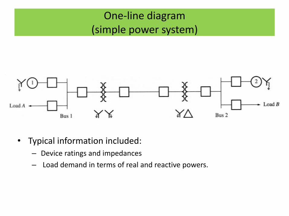
One-line diagram (simple power system)

• Typical information included: – Device ratings and impedances

– Load demand in terms of real and reactive powers.

Per-unit equivalent circuit

• Real power systems are convenient to analyze using their per-phase (since its is a balanced three-phase) per-unit (since there are many transformers) equivalent circuits.

• Recall: given the base apparent power (3—phase) and base voltage (line-to-line), the base current and base impedance are given by

Per-unit system

• The base apparent power and base voltage are specified at a point in the circuit, and the other values are calculated from them.

• The base voltage varies by the voltage ratio of each transformer in the circuit but the base apparent power stays the same through the circuit.

• The per-unit impedance may be transformed from one base to another as

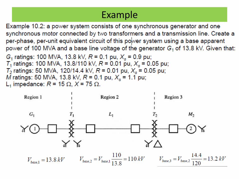
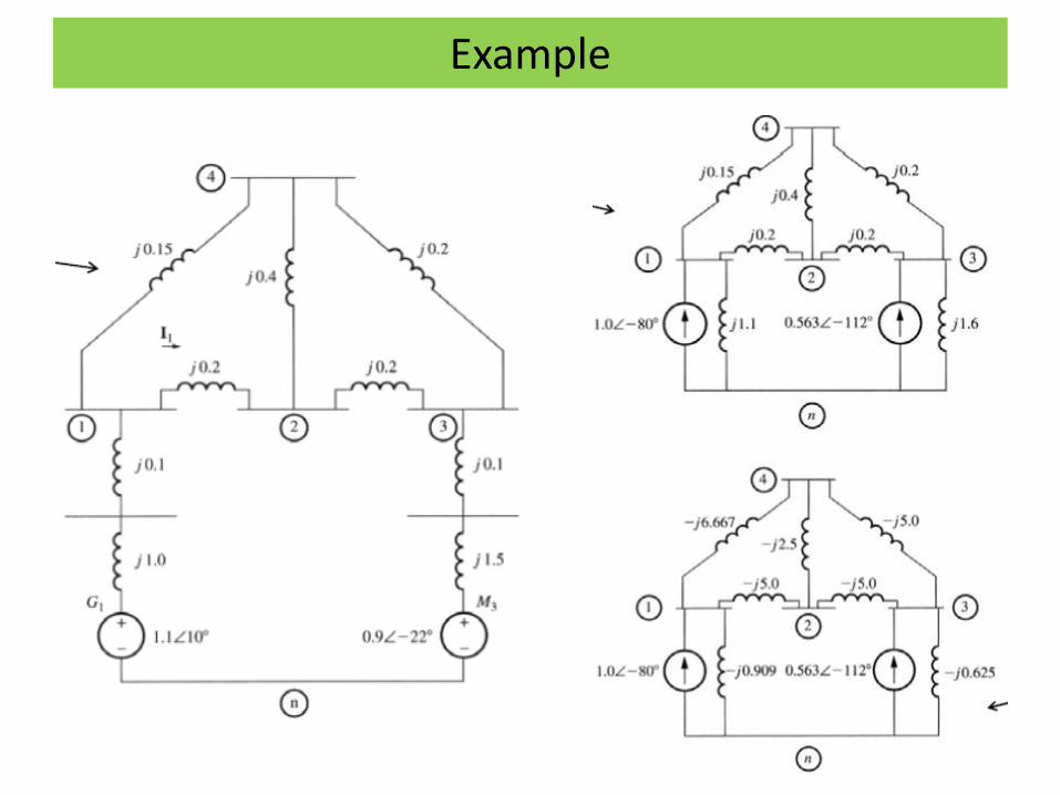
Example

Example (cont.)

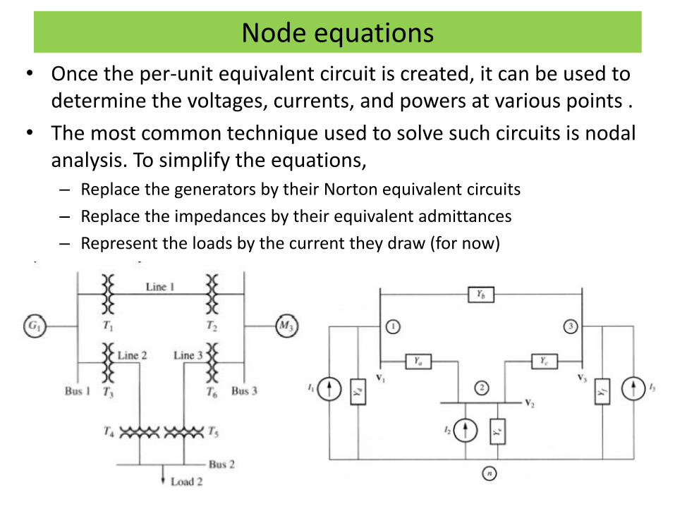
Node equations

• Once the per-unit equivalent circuit is created, it can be used to determine the voltages, currents, and powers at various points .

• The most common technique used to solve such circuits is nodal analysis. To simplify the equations, – Replace the generators by their Norton equivalent circuits

– Replace the impedances by their equivalent admittances

– Represent the loads by the current they draw (for now)

Node equations

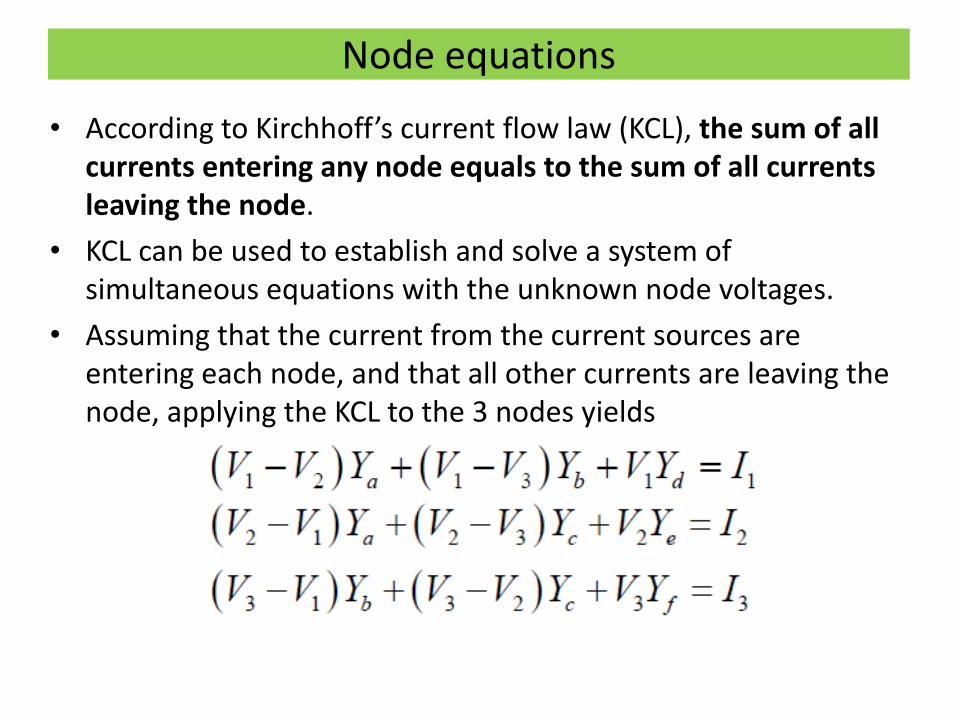
• According to Kirchhoff’s current flow law (KCL), the sum of all currents entering any node equals to the sum of all currents leaving the node.

• KCL can be used to establish and solve a system of simultaneous equations with the unknown node voltages.

• Assuming that the current from the current sources are entering each node, and that all other currents are leaving the node, applying the KCL to the 3 nodes yields

Node equations – the Ybus matrix

• In matrix from,

Ybus and Zbus matrices of a power network

Example

Example (cont.)

Problems

• 10.3

• 10.5

• 10.7, 10.8, 10.9

Power-flow analysis equations

11 12 13 14 1 1

21 22 23 24 2 2

31 32 33 34 3 3

41 42 43 44 4 4

Y Y Y Y V I

Y Y Y Y V I

Y Y Y Y V I

Y Y Y Y V I

The basic equation for power-flow analysis is derived from

the nodal analysis equations for the power system: For

example, for a 4-bus system,

where Yij are the elements of the bus admittance matrix, Vi are

the bus voltages, and Ii are the currents injected at each node.

The node equation at bus i can be written as

n

j

jiji VYI1

Power-flow analysis equations

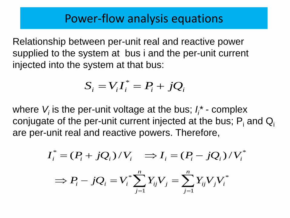
Relationship between per-unit real and reactive power

supplied to the system at bus i and the per-unit current

injected into the system at that bus:

where Vi is the per-unit voltage at the bus; Ii* - complex

conjugate of the per-unit current injected at the bus; Pi and Qi

are per-unit real and reactive powers. Therefore,

iiiii jQPIVS *

** /)(/)( iiiiiiii VjQPIVjQPI

n

j

ijij

n

j

jijiii VVYVYVjQP1

*

1

*

Power flow equations

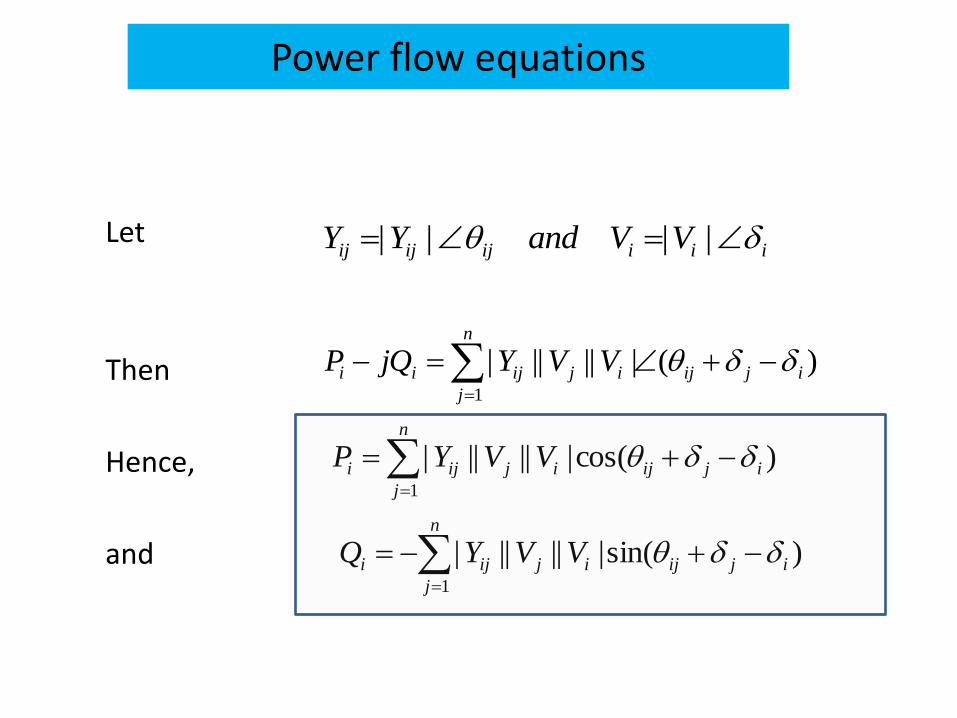
Let

Then

Hence,

and

iiiijijij VVandYY ||||

)(||||||1

ijij

n

j

ijijii VVYjQP

)cos(||||||1

ijij

n

j

ijiji VVYP

)sin(||||||1

ijij

n

j

ijiji VVYQ

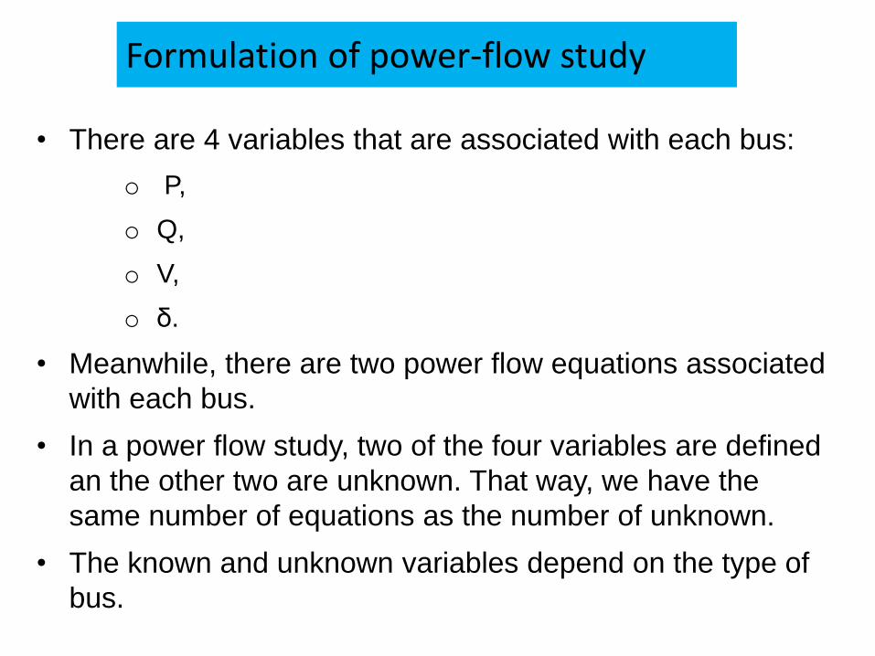
• There are 4 variables that are associated with each bus:

o P,

o Q,

o V,

o δ.

• Meanwhile, there are two power flow equations associated

with each bus.

• In a power flow study, two of the four variables are defined

an the other two are unknown. That way, we have the

same number of equations as the number of unknown.

• The known and unknown variables depend on the type of

bus.

Formulation of power-flow study

Each bus in a power system can be classified as one of three types:

1. Load bus (P-Q bus) – a buss at which the real and reactive

power are specified, and for which the bus voltage will be

calculated. All busses having no generators are load busses. In

here, V and δ are unknown.

2. Generator bus (P-V bus) – a bus at which the magnitude of the

voltage is defined and is kept constant by adjusting the field

current of a synchronous generator. We also assign real power

generation for each generator according to the economic

dispatch. In here, Q and δ are unknown

3. Slack bus (swing bus) – a special generator bus serving as the

reference bus. Its voltage is assumed to be fixed in both

magnitude and phase (for instance, 10˚ pu). In here, P and Q

are unknown.

Formulation of power-flow study

Formulation of power-flow study

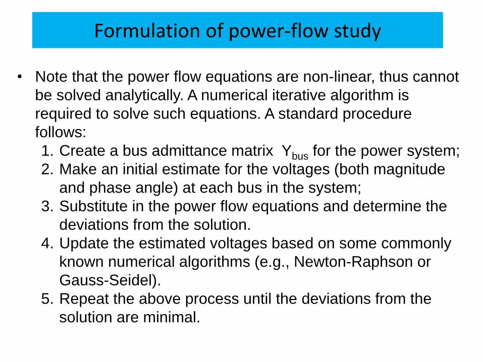
• Note that the power flow equations are non-linear, thus cannot

be solved analytically. A numerical iterative algorithm is

required to solve such equations. A standard procedure

follows:

1. Create a bus admittance matrix Ybus for the power system;

2. Make an initial estimate for the voltages (both magnitude

and phase angle) at each bus in the system;

3. Substitute in the power flow equations and determine the

deviations from the solution.

4. Update the estimated voltages based on some commonly

known numerical algorithms (e.g., Newton-Raphson or

Gauss-Seidel).

5. Repeat the above process until the deviations from the

solution are minimal.

Example

Consider a 4-bus power system below. Assume that

– bus 1 is the slack bus and that it has a voltage V1 = 1.0∠0° pu.

– The generator at bus 3 is supplying a real power P3 = 0.3 pu to the system with a voltage magnitude 1 pu.

– The per-unit real and reactive power loads at busses 2 and 4 are P2 = 0.3 pu, Q2 = 0.2 pu, P4 = 0.2 pu, Q4 = 0.15 pu.

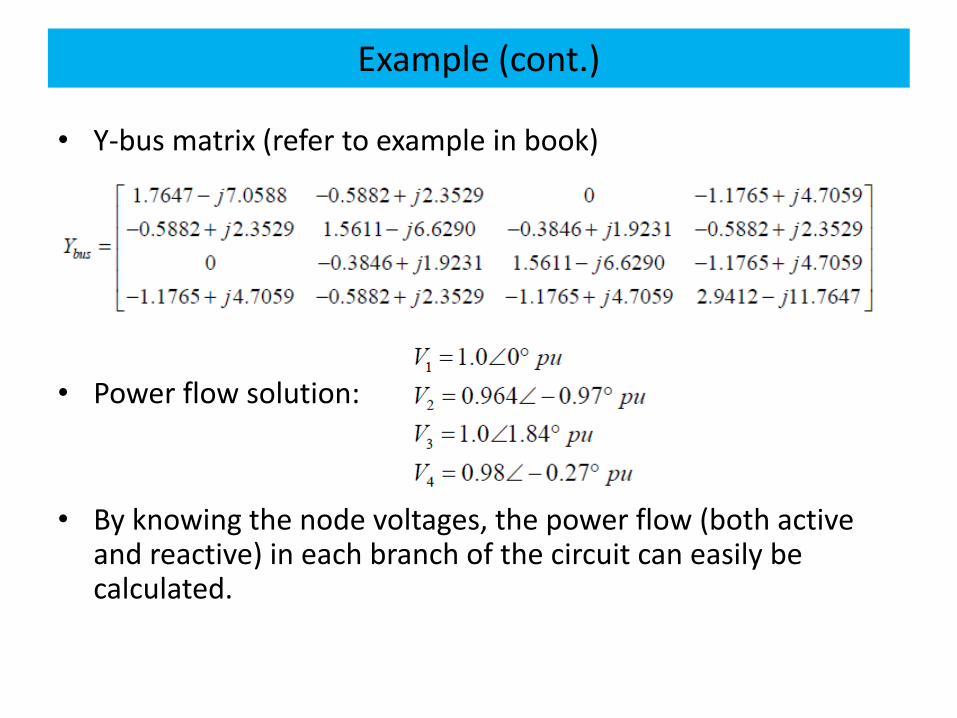
Example (cont.)

• Y-bus matrix (refer to example in book)

• Power flow solution:

• By knowing the node voltages, the power flow (both active and reactive) in each branch of the circuit can easily be calculated.