arX

iv:s

ubm

it/11

7861

9 [c

s.IT

] 7

Feb

201

51

Power Efficient Resource Allocation for

Full-Duplex Radio Distributed Antenna

Networks

Derrick Wing Kwan Ng, Yongpeng Wu, and Robert Schober

Abstract

In this paper, we study the resource allocation algorithm design for distributed antenna multiuser

networks with full-duplex (FD) radio base stations (BSs) which enable simultaneous uplink and downlink

communications. The considered resource allocation algorithm design is formulated as an optimiza-

tion problem taking into account the antenna circuit power consumption of the BSs and the quality

of service (QoS) requirements of both uplink and downlink users. We minimize the total network

power consumption by jointly optimizing the downlink beamformer, the uplink transmit power, and

the antenna selection. To overcome the intractability of the resulting problem, we reformulate it as

an optimization problem with decoupled binary selection variables and non-convex constraints. The

reformulated problem facilitates the design of an iterative resource allocation algorithm which obtains

an optimal solution based on the generalized Bender’s decomposition (GBD) and serves as a benchmark

scheme. Furthermore, to strike a balance between computational complexity and system performance, a

suboptimal algorithm with polynomial time complexity is proposed. Simulation results illustrate that the

proposed GBD based iterative algorithm converges to the global optimal solution and the suboptimal

algorithm achieves a close-to-optimal performance. Our results also demonstrate the trade-off between

power efficiency and the number of active transmit antennas when the circuit power consumption is

taken into account. In particular, activating an exceedingly large number of antennas may not be a power

efficient solution for reducing the total system power consumption. In addition, our results reveal that

FD systems facilitate significant power savings compared totraditional half-duplex systems, despite the

non-negligible self-interference.

Index Terms

Distributed antennas, full-duplex radio, antenna selection, non-convex optimization, resource allo-

cation.

Derrick Wing Kwan Ng, Yongpeng Wu, and Robert Schober are with the Institute for Digital Communications (IDC), Friedrich-

Alexander-University Erlangen-Nurnberg (FAU), Germany(email:kwan, yongpeng.wu, schober@lnt.de). Derrick Wing Kwan

Ng and Robert Schober are also with the University of BritishColumbia, Vancouver, Canada.

2

I. INTRODUCTION

The next generation wireless communication systems are required to support ubiquitous and

high data rate communication applications with guaranteedquality of service (QoS). These re-

quirements translate into a tremendous demand for bandwidth and energy consumption. Multiple-

input multiple-output (MIMO) is a viable solution for addressing these issues as it provides extra

degrees of freedom in the spatial domain which facilitates atrade-off between multiplexing gain

and diversity gain. Hence, a large amount of work has been devoted to MIMO communication

over the past decades [1], [2]. However, the modest computational capabilities of mobile devices

limit the MIMO gains that can be achieved in practice. An attractive alternative for realizing

the performance gains offered by multiple antennas is multiuser MIMO, where a multiple-

antenna transmitter serves multiple single-antenna receivers simultaneously [3], [4]. In fact, the

combination of multiuser MIMO and distributed antennas is widely recognized as a promising

technology for mitigating interference and extending service coverage [5]–[7]. Specifically, dis-

tributed antennas introduce additional capabilities for combating both path loss and shadowing by

shortening the distances between the transmitters and the receivers. Nevertheless, if the number

of antennas is very large, the circuit power consumption of distributed antenna networks becomes

non-negligible compared to the power consumed for transmission. However, this problem has

not been considered in most of the existing literature [5]–[7] on power efficient communication

network design. Furthermore, even with these powerful MIMOtechniques, spectrum scarcity is

still a major obstacle in providing high speed uplink and downlink communications.

Traditional communication systems are designed for half-duplex (HD) transmission since

this mode of operation facilitates low-complexity transceiver design. In particular, uplink and

downlink communication are statically separated in eithertime or frequency, e.g. via time division

duplex or frequency division duplex, which leads to a loss inspectral efficiency. Even though

different approaches have been proposed for improving the spectral efficiency of HD systems, e.g.

dynamic uplink-dowlink scheduling/allocation in time division duplex communication systems

[8], [9], the fundamental spectral efficiency loss induced by the HD constraint remains unsolved.

On the contrary, full duplex (FD) transmission allows downlink and uplink transmission to occur

simultaneously at the same frequency. In fact, FD radio has the potential to double the spectral

efficiency of conventional HD communication systems. However, in practice, the downlink

3

transmission in FD systems creates self-interference to the uplink receive antennas which can be

exceedingly large compared to the received power of the useful information signals. In fact, the

huge difference in the power levels of the two signals saturates the dynamic range of the analog-

to-digital converter (ADC) essentially preventing FD communication. Fortunately, several recent

breakthroughs in hardware (/signal processing algorithm)design for suppressing self-interference

have been reported and FD radio prototypes have been successfully presented [10]–[14]. As a

result, FD radio has regained the attention of both industry[15]–[18] and academia [19]–[23].

In [19], the authors studied techniques for self-interference suppression and cancellation for FD

multiple-antenna relays. In [20], the outage probability of MIMO FD single-user relaying systems

was investigated. In [21], a resource allocation algorithmwas proposed for maximization of the

achievable end-to-end system data rate of multicarrier multiuser MIMO FD relaying systems.

In [22], a suboptimal beamformer design was considered to improve the spectral efficiency of a

FD radio base station enabling simultaneous uplink and downlink communication. In [23], the

concept of FD communication was extended to the case of massive MIMO where a FD radio

relay is equipped with a large number of antennas for suppressing the self-interference and for

enhancing the system throughput. However, the benefits of multiple-antenna FD radio do not

come for free. The rapidly escalating cost caused by the power consumption of the circuitries of

large antenna systems has lead to significant financial implications for service providers, which is

often overlooked in the literature [10]-[23]. In fact, the systems in [10]-[23] are designed to serve

peak service demands by activating all available antennas of the system, without considering the

power consumption in the off-peak periods. However, the service loads vary across a wireless

network in practice, depending on the geographic location of the receivers and the time of day.

Thus, we expect that extra power savings can be achieved by dynamically switching off some of

the antennas. Nevertheless, the optimal number of active antennas has not been investigated from

a system power efficiency point of view for FD radio communication, yet. In addition, there

may be fewer degrees of freedom for self-interference suppression at each FD radio base station

in distributed antenna systems if the total number of antennas in the network is fixed. Thus,

it is unclear whether the distributed antenna architectureleads to power savings for FD radio

communication. Furthermore, unlike for the orthogonal transmission adopted in HD systems,

the uplink and downlink transmit powers are coupled in FD systems which make the design of

efficient resource allocation algorithms particularly challenging.

4

In this paper, we address the above issues and study the resource allocation algorithm design for

multiuser distributed antenna communication networks. Weminimize the total network power

consumption while taking into account the circuit power consumption of the distributed BS

antennas and ensuring the QoS of both uplink and downlink users. In particular, we propose an

optimal iterative resource allocation algorithm based on the generalized Bender’s decomposition

[24]–[26]. Furthermore, we propose a suboptimal resource allocation scheme with polynomial

time computational complexity based on the difference of convex functions (d.c.) programming

[27] which finds a local optimal solution for the considered optimization problem.

II. SYSTEM MODEL

A. Notation

Matrices and vectors are represented by boldface capital and lower case letters, respectively.

AH , AT , Tr(A), andRank(A) represent the Hermitian transpose, the transpose, the trace, and

the rank of matrixA, respectively;A ≻ 0 andA 0 indicate thatA is a positive definite and a

positive semidefinite matrix, respectively;IN is theN×N identity matrix;CN×M andHN denote

the sets of allN×M matrices andN×N Hermitian matrices with complex entries, respectively;

diag(x1, · · · , xK) denotes a diagonal matrix with the diagonal elements given by x1, · · · , xK;

|·| denotes the absolute value of a complex scalar; the circularly symmetric complex Gaussian

distribution is denoted byCN (µ,C) with mean vectorµ and co-variance matrixC; ∼ stands for

“distributed as”;E· denotes statistical expectation; and∇xf denotes the gradient of a function

f with respect to vectorx.

B. System Model

We consider a distributed antenna multiuser communicationnetwork. The system consists of

a central processor (CP),L FD radio base stations (BSs), andK mobile users, cf. Figure 1. Each

FD radio BS is equipped withNT > 1 antennas for downlink transmission and uplink reception1.

TheK users employ single-antenna HD mobile communication devices to ensure low hardware

complexity. In particular,KU andKD users are scheduled for simultaneous uplink and downlink

transmission, respectively, such thatKU+KD = K. On the other hand, the CP is the core unit of

the network. In particular, the FD radios are connected to the CP via backhaul links. In addition,

1We assume that the antennas equipped at the FD BSs can transmit and receive simultaneously which has been successfully

demonstrated in some FD radio prototypes [12].

5

FD radio BS 2

Downlink user 1

Uplink user 1

FD radio BS 3

FD radio BS 1

Signal

Co-channel Interference Central processor

(CP)

Backhaul connection

Fig. 1. Multiuser downlink distributed antenna communication system model withL = 3 full duplex (FD) radio base stations

(BSs),KU = 1 uplink user, andKD = 1 downlink user. For the depicted case, the antennas equippedat FD radio BS2 are

switched to idle mode for reducing the total power consumption in the network.

the CP has the full channel state information of the entire network and the data of all downlink

users for resource allocation. In this paper, we assume thatthe CP is a powerful computing unit,

e.g. a series of baseband units as in cloud radio access networks (C-RAN), which computes the

resource allocation policy and broadcasts it to all FD radioBSs. Each FD radio BS receives the

control signals for resource allocation and the data of theKD downlink users from the CP via a

backhaul link. Furthermore, the FD radio BSs transfer the received uplink signals via backhaul

links to the CP, where the information is decoded. In this paper, we assume that the backhaul

links are implemented with optical fiber and have sufficiently large capacity and low latency to

support real time information exchange between the CP and the FD radio BSs. For studies on

the impact of a limited backhaul capacity on the performanceof wireless systems, please refer

to [2], [28].

C. Channel Model

A frequency flat fading channel is assumed2 in this paper. The received signals at downlink

userk ∈ 1, . . . , KD and theL FD radio BSs are given by

yDLk = hH

Dkx +

KU∑

j=1

√PUj gj,kd

Uj

︸ ︷︷ ︸co−channel interference

+nk and (1)

yUL =

KU∑

j=1

PUj hUj

dUj + HSIx︸ ︷︷ ︸self−interference

+z, (2)

2The frequency flat fading channel can be interpreted as one subcarrier of an orthogonal frequency division multiplexing

system.

6

respectively, wherex ∈ CNTL×1 denotes the joint transmit signal vector of theL FD radio BSs to

theKD downlink users. The downlink channel between theL FD radio BSs and userk is denoted

by hDk∈ CNTL×1, and we usegj,k ∈ C to represent the channel between uplink userj and

downlink userk. dUj andPUj are the transmit data and transmit power sent from uplink user j to

theL FD radio BSs, respectively.hUj∈ CNTL×1 is the uplink channel between uplink userj and

theL FD radio BSs. Due to simultaneous uplink reception and downlink transmission at the FD

radio BSs, self-interference from the downlink impairs theuplink signal reception. In practice,

different interference mitigation techniques such as antenna cancellation, balun cancellation, and

circulators [12], [13] have been proposed to alleviate the impairment caused by self-interference.

In order to isolate the resource allocation algorithm design from the specific implementation of

self-interference mitigation, we model the residual self-interference after interference cancellation

by matrix HSI ∈ CNTL×NTL. VariableshDk, gj,k, HSI, andhUj

capture the joint effect of path

loss and multipath fading.z ∼ CN (0, σ2zINTL) andnk ∼ CN (0, σ2

nk) represent the additive white

Gaussian noise (AWGN) at theL FD radio BSs and userk, respectively.

In each scheduling time slot,KD independent signal streams are transmitted simultaneously at

the same frequency to theKD downlink users. Specifically, a dedicated downlink beamforming

weight, wlk ∈ C, is allocated to downlink userk at the l-th, l ∈ 1, . . . , NTL, antenna to

facilitate downlink information transmission. For the sake of presentation, we define a super-

vectorwk ∈ CNTL×1 for downlink userk as

wk =[w1

k w2k . . . w

NTLk

]T. (3)

wk represents the joint beamformer used by theNTL antennas shared by the FD radio BSs for

serving downlink userk. Then, the information signal to downlink userk, xk, can be expressed

as

xk = wkdDk , (4)

wheredDk ∈ C is the data symbol for downlink userk. Without loss of generality, we assume

that E|dDk |2 = E|dUj |

2 = 1, ∀k ∈ 1, . . . , KD, j ∈ 1, . . . , KU.

D. Network Power Consumption Model

In our system model, we include the circuit power consumption of the system in the objec-

tive function in order to design a resource allocation algorithm which facilities power-efficient

7

communication. Thus, we model the power dissipation in the system as the sum of one static

term and four dynamic terms as follows [24]:

UTP

(wk, sl, P

Uj

)= P0 +

NTL∑

l=1

slPActive +

NTL∑

l=1

(1− sl)PIdle

︸ ︷︷ ︸Antenna power consumption

+ η

NTL∑

l=1

KD∑

k=1

εD|wlk|

2 +

KU∑

j=1

εUζjPUj

︸ ︷︷ ︸Amplifer power consumption

, (5)

whereP0 is the aggregated static power consumption of the CP, all FD radio BSs, and all backhaul

links. sl ∈ 0, 1 is a binary selection variable. In particular,sl = 1 and sl = 0 indicate that

the l-th antenna in the FD communication system is in active mode and idle mode, respectively,

sl will be optimized to minimize the total network power consumption in the next section.

PActive > 0 is the signal processing power that is consumed if an antennais active.PActive

includes the power dissipations of the transmit filter, mixer, frequency synthesizer, digital-to-

analog converter, etc. In this paper, an FD radio antenna is considered active if it serves at least

one user in the system.P Idle > 0 is the required power consumption of an antenna in idle mode,

i.e., if it is not serving any user, andPActive > P Idle holds in general.∑KD

k=1

∑NTL

l=1 |wlk|

2 is the

total power radiated by theL FD radio BSs for downlink transmission.εD ≥ 1 and εU ≥ 1

are constants which account for the inefficiency of the poweramplifier 3 adopted for downlink

and uplink transmission, respectively. In other words,εD∑KD

k=1

∑NTL

l=1 |wlk|

2 andεU∑KU

j=1 PUj are

the total power consumptions of the power amplifiers for downlink and uplink transmission,

respectively.η ≥ 0 and ζj ≥ 0 in the last two terms of (5) are constant weights which can be

chosen by the system designer to prioritize the importance of the total downlink transmit power

and the transmit power of individual uplink usersj ∈ 1, . . . , KU, respectively.

III. PROBLEM FORMULATION

In this section, we first introduce the QoS metrics for the considered FD radio communi-

cation network. Then, we formulate the resource allocationalgorithm design as a non-convex

optimization problem.

3We assume Class A power amplifiers with linear characteristic are implemented in the transceivers. In practice, the maximum

power efficiency of Class A amplifiers is25%.

8

A. Achievable Data Rate

The achievable data rate (bit/s/Hz) between theL FD radio BSs and downlink userk ∈

1, . . . , KD is given by

Ck = log2(1 + ΓDLk ), where ΓDL

k =|hH

Dkwk|2

KD∑t6=k

|hHDkwt|2 +

∑KU

j=1 PUj |gj,k|

2 + σ2nk

(6)

is the receive signal-to-interference-plus-noise ratio (SINR) at downlink userk.

On the other hand, we assume that the CP employs a linear receiver for decoding of the

received uplink information. Therefore, the achievable data rate between theL FD radio BSs

and uplink userj is given by

CULj = log2

(1 + ΓUL

j

), ΓUL

j =PUj |vH

j hUj|2

σ2z‖vj‖2 + Ij

, (7)

Ij = vHj

( KD∑

k=1

HSIwkwHk H

HSI

)vj +

KU∑

r 6=j

PUr |v

Hj hUr

|2, (8)

wherevj ∈ CNTL×1 is the receive beamforming vector for decoding of the information for uplink

userj. In this paper, maximum ratio combining (MRC) is adopted, i.e., the receive beamformer

for uplink userj is chosen asvj =∑NTL

l=1 slRlhUjto maximize the signal strength of the received

signal, whereRl , diag(0, · · · , 0︸ ︷︷ ︸

(l−1)

, 1, 0, · · · , 0︸ ︷︷ ︸LNT−l

), ∀l ∈ 1, . . . , LNT, is a diagonal matrix. It is

known that MRC achieves a good system performance, especially if a large number of antennas

is employed, and has been widely adopted in the literature [3], [4].

Remark 1: We note that zero-forcing beamforming (ZFBF) or minimum mean square error

beamforming (MMSE-BF) are not considered for uplink signaldetection since they do not

facilitate an efficient resource allocation algorithm design for the considered network.

Using MRC, the uplink SINR of userj is given by

ΓULj =

PUj Tr

(hUj

hHUj

∑NTL

m=1

∑NTL

n=1 smsnRmhUjhHUjRH

n

)

σ2z Tr

(∑NTL

l=1 slhUjhHUjRl

)+ Ij

, where (9)

Ij = Tr( KD∑

k=1

HSIwkwHk H

HSI

NTL∑

m=1

NTL∑

n=1

smsnRmhUjhHUjRH

n

)(10)

+

KU∑

r 6=j

PUr Tr

(hUr

hHUr

NTL∑

m=1

NTL∑

n=1

smsnRmhUjhHUjRH

n

). (11)

9

B. Optimization Problem Formulation

The system objective is to minimize the total network power consumption while providing

QoS for reliable communication to both uplink and downlink users simultaneously. We obtain

the optimal resource allocation algorithm policy by solving the following optimization problem:

minimizewk,sl,P

Uj

UTP

(wk, sl, P

Uj

)

s.t. C1:|hH

Dkwk|2

KD∑t6=k

|hHDkwt|2 +

∑KU

j=1 PUj |gj,k|2 + σ2

nk

≥ ΓDLreqk

, ∀k ∈ 1, . . . , KD,

C2: ΓULj ≥ ΓUL

reqj, ∀j ∈ 1, . . . , KU,

C3:KD∑

k=1

|wlk|

2 ≤ slPDLmaxl

, ∀l ∈ 1, . . . , NTL, C4: 0 ≤ PUj ≤ PU

maxj, ∀j ∈ 1, . . . , KU,

C5: sl ∈ 0, 1, ∀l ∈ 1, . . . , NTL. (12)

ΓDLreqk

andΓULreqj

in constraints C1 and C2 denote the minimum receive SINR required by downlink

userk and uplink userj for successful information decoding, respectively. In C3,we constrain

the maximum radiated power of thel-th antenna in the system toPDLmaxl

to satisfy the maximum

power spectral mask limit. C4 limits the maximum transmit power and ensures the non-negativity

of the transmit power of uplink userj. C5 constrains the optimization variables which control

the active and idle states of the antennas in the system to be binary.

Remark 2: In this paper, energy/power saving is achieved by optimizing not only the uplink

and downlink transmit powers, but also by optimizing the states of the antennas in the network.

Thereby, it is expected that switching the antennas on and off adaptively according to the channel

conditions is an effective strategy for reducing the network power consumption when the QoS

requirements are not stringent or the number of users is low.

IV. RESOURCEALLOCATION ALGORITHM DESIGN

The optimization problem in (12) is a mixed non-convex and combinatorial optimization

problem. The combinatorial nature is due to the binary selection variables in C5. Also, variable

sl is coupled with both downlink beamforming vectorwk and uplink power allocation variable

PUj in constraint C2. Furthermore, constraint C1 is non-convexwith respect towk. In the

following, we first transform the optimization problem intoan equivalent form and obtain the

10

global optimal solution by using the generalized Bender’s decomposition. Then, we propose a

suboptimal polynomial time algorithm which is inspired by the difference of convex functions

program.

A. Problem Reformulation

In this section, we reformulate the considered optimization problem in (12) using the defini-

tionsWk = wkwHk , HDk

= hDkhHDk

, andHUj= hUj

hHUj

. This leads to

minimizeWk∈H

NTL,sl,PUj ,qm,n

P0 +

NTL∑

l=1

slPActive +

NTL∑

l=1

(1− sl)PIdle + η

KD∑

k=1

εDTr(Wk) + εU

KU∑

j=1

ζjPUj

s.t. C1:Tr(HDk

Wk)

ΓDLreqk

≥KD∑

t6=k

Tr(HDkWj) +

KU∑

j=1

PUj |gj,k|

2 + σ2nk, ∀k,

C2:PUj

ΓULreqj

Tr(HUj

NTL∑

m=1

NTL∑

n=1

qm,nRmHUjRH

n

)

≥ σ2z Tr

(NTL∑

l=1

ql,lHUjRl

)+ Tr

( KD∑

k=1

HSIWkHHSI

NTL∑

m=1

NTL∑

n=1

qm,nRmHUjRH

n

)

+∑

r 6=j

Tr(HUr

NTL∑

m=1

NTL∑

n=1

PUr qm,nRmHUj

RHn

), ∀j ∈ 1, . . . , KU,

C3:KD∑

k=1

Tr(WkRl) ≤ slPDLmaxl

, ∀l ∈ 1, . . . , NTL, C4, C5,

C6: Wk 0, ∀k, C7: Rank(Wk) ≤ 1, ∀k,C8: 0 ≤ qm,n ≤ sm, ∀m,n ∈ 1, . . . , NTL,

C9: qm,n ≤ sn, ∀m,n, C10: qm,n ≥ sn + sm − 1, ∀m,n. (13)

Constraints C6, C7, andWk ∈ HNTL, ∀k, are imposed to guarantee thatWk = wkw

Hk holds

after optimization.qm,n is an auxiliary continuous optimization variable which is introduced to

handle the product of two binary variablessnsm in constraint C2, cf. (9)–(11). In particular,

because of constraints C8 – C10,qm,n will have a binary value ifsl is binary.

We note that constraint C2 is still non-convex due to the product termsqm,nPUt andqm,nWk

which is an obstacle for the design of a computationally efficient resource allocation algorithm.

In order to circumvent this difficulty, we adopt the big-M formulation [29], [30] to decompose

the product terms. First, we introduce auxiliary variablesPUj,m,n = PU

j qm,n andWm,n

k = Wkqm,n.

11

Then, we impose the following additional constraints:

C11: PUj,m,n ≤ PU

maxjqm,n, ∀j,m, n, C12: PU

j,m,n ≤ PUj , ∀j,m, n, (14a)

C13: PUj,m,n ≥ PU

j − (1− qm,n)PUmaxj

, ∀j,m, n, C14: PUj,m,n ≥ 0, (14b)

C15: Wm,n

k INTLPDLmaxl

qm,n, ∀k,m, n, C16: Wm,n

k Wk, ∀k,m, n, (14c)

C17: Wm,n

k Wk − (1− qm,n)INTLPDLmaxl

, ∀k,m, n,C18: Wm,n

k 0, ∀k,m, n. (14d)

In particular, constraints C11-C18 involve only continuous optimization variables, i.e.,Pj, Pj,m,n,

qm,n, andWk, which facilitates the design of an efficient resource allocation algorithm. Subse-

quently, we substitutePUj,m,n = PU

j qm,n andWm,n

k = Wkqm,n into the coupled variables in C2

which yields

C2:1

ΓULreqj

Tr(HUj

NTL∑

m=1

NTL∑

n=1

PUj,m,nRmHUj

RHn

)

≥ σ2z Tr

(NTL∑

l=1

ql,lHUjRl

)+ Tr

( KD∑

k=1

NTL∑

m=1

NTL∑

n=1

HSIWm,n

k HHSIRmHUj

RHn

)

+∑

r 6=j

Tr(HUr

NTL∑

m=1

NTL∑

n=1

PUr,m,nRmHUj

RHn

), ∀j ∈ 1, . . . , KU. (15)

The big-M formulation linearizes the termsqm,nPUr andqm,nWk such that constraintC2 is an

affine function with respect to the new optimization variables PUj,m,n and W

m,n

k . We note that

constraints C2 andC2 are equivalent when constraints C5 and C11–C18 are satisfied.

As a result, the considered optimization problem (13) can betransformed into the following

equivalent problem:

minimizeWk∈H

NTL,Wm,n

k,sl,qm,n,

PUj

,PUj,m,n

P0 +

NTL∑

l=1

slPActive +

NTL∑

l=1

(1− sl)PIdle + η

KD∑

k=1

εDTr(Wk) +

KU∑

j=1

εUζjPUj

s.t. C1, C2,C3, C4, C6,C8 – C18,

C5: sl ∈ 0, 1, ∀l, C7: Rank(Wk) ≤ 1, ∀k, (16)

and we can focus on the design of an algorithm for solving the optimization problem in (16).

Now, the remaining non-convexity of optimization problem (16) is due to constraints C5 and

C7.

Remark 3: We note that the uplink-downlink duality approach in [31], [32] cannot be applied

to our problem for the following two reasons. First, the uplink and downlink transmit power

12

variables are coupled in constraints C1 and C2. Second, the uplink and downlink transmit powers

of each transceiver are constrained.

B. Optimal Iterative Resource Allocation Algorithm

Now, we adopt the generalized Bender’s decomposition (GBD)to handle the constraints

involving binary optimization variables [24]–[26], i.e.,C3, C8, C9, and C10. In particular, we de-

compose the problem in (16) into two sub-problems:(a) a primal problem which is a non-convex

optimization problem involving continuous optimization variablesWk,Wm,n

k , PUj , P

Uj,m,n, qm,n;

(b) a master problem which is a mixed integer linear program (MILP). Specifically, the primal

problem is solved for givensl which yields an upper bound for the optimal value of (16). In

contrast, the solution of the master problem provides a lower bound for the optimal value of (16).

Subsequently, we solve the primal and master problems iteratively until the solutions converge.

In the following, we first propose algorithms for solving theprimal and master problems in the

i-th iteration, respectively. Then, we describe the iterative procedure between the master problem

and the primal problem.

1) Solution of the primal problem in the i-th iteration: For given and fixed input parameters

sl = sl(i) obtained from the master problem in thei-th iteration, we minimize the objective

function with respect to variablesWk,Wm,n

k , PUj , P

Uj,m,n, qm,n in the primal problem:

minimizeWk∈H

NTL,Wm,n

k,qm,n,

PUj

,PUj,m,n

P0 +

NTL∑

l=1

slPActive +

NTL∑

l=1

(1− sl)PIdle + η

KD∑

k=1

εDTr(Wk) + εU

KU∑

j=1

ζjPUj

s.t. C1, C2,C3, C4, C16 – C18. (17)

We note that constraint C5 in (16) will be handled by the master problem since it involves only

the binary optimization variablesl. Now, the only obstacle in solving (17) is the combinatorial

rank constraint in C7 and we adopt the SDP relaxation approach to handle this non-convexity. In

particular, we relax constraint C7:Rank(Wk) ≤ 1 by removing it from the problem formulation,

such that the considered problem in (17) becomes a convex SDPand can be solved efficiently

by numerical methods designed for convex programming such as interior point methods [33].

If the solutionWk of the relaxed version of (17) is a rank-one matrix for all downlink users,

then the problem in (17) and its relaxed version share the same optimal solution and the same

optimal objective value.

13

Now, we study the tightness of the adopted SDP relaxation. The SDP relaxed version of

(17) is jointly convex with respect to the optimization variables and satisfies Slater’s constraint

qualification. Thus, strong duality holds and solving the dual problem is equivalent to solving

(17). To obtain the dual problem, we define the Lagrangian of the relaxed version of (17) as

L(Θ,Φ

)= UTP

(Wk, sl, P

Uj

)+f1(Θ,Φ)+f2(Θ,Φ), where (18)

UTP

(Wk, sl, P

Uj

)= P0+

NTL∑

l=1

slPActive+

NTL∑

l=1

(1− sl)PIdle + η

KD∑

k=1

εDTr(Wk)+εU

KU∑

j=1

ζjPUj (19)

f1(Θ,Φ) = −KD∑

k=1

Tr(ZkWk)−KU∑

j=1

NTL∑

m=1

NTL∑

n=1

βj,m,nPUj,m,n +

KU∑

j=1

λj(PUj − PU

maxj)

+

KD∑

k=1

αk

[−

Tr(HDkWk)

ΓDLreqk

+

KD∑

t6=k

Tr(HDkWj) +

KU∑

j=1

PUj |gj,k|

2 + σ2z

]−

KU∑

j=1

χjPUj

+

KU∑

j=1

ψj

(−Tr

(HUj

∑NTL

m=1

∑NTL

n=1 PUj,m,nRmHUj

RHn

)

ΓULreqj

+ σ2z Tr

(NTL∑

l=1

ql,lHUjRl

)

+Tr( KD∑

k=1

NTL∑

m=1

NTL∑

n=1

HSIWm,n

k HHSIRmHUj

RHn

)+∑

r 6=j

Tr(HUr

NTL∑

m=1

NTL∑

n=1

PUr,m,nRmHUj

RHn

))

+

KU∑

j=1

NTL∑

m=1

NTL∑

n=1

µj,m,n(PUj,m,n − PU

maxjqm,n) +

KU∑

j=1

NTL∑

m=1

NTL∑

n=1

ξj,m,n

(PUj − (1− qm,n)P

Umaxj

− PUj,m,n

)

+

KU∑

j=1

NTL∑

m=1

NTL∑

n=1

τj,m,n(PUj,m,n − PU

j )−NTL∑

m=1

NTL∑

n=1

ςm,nqm,n

+

KD∑

k=1

NTL∑

m=1

NTL∑

n=1

Tr

DC15k,m,n

(W

m,n

k − INTLPDLmaxl

qm,n

)+DC16k,m,n

(W

m,n

k −Wk

)

+

KD∑

k=1

NTL∑

m=1

NTL∑

n=1

Tr

DC17k,m,n

(Wk−(1 − qm,n)INTLP

DLmaxl

−Wm,n

k

)−DC18k,m,n

Wm,n

k

, and (20)

f2(Θ,Φ) =

KD∑

k=1

NTL∑

l=1

ρl

(Tr(WkRl)− slP

DLmaxl

)+

NTL∑

m=1

NTL∑

n=1

κm,n(qm,n − sm)

+

NTL∑

m=1

NTL∑

n=1

ϕm,n(qm,n − sn) +

NTL∑

m=1

NTL∑

n=1

ωm,n(sn + sm − 1− qm,n). (21)

Here,Θ = Wk, sl, PUj ,W

m,n

k , PUj,m,n, qm,n andΦ = αk, ψj, ρl, λj, χj,Zk, ςm,n, κm,n, ϕm,n,

ωm,n, µj,m,nτj,m,n, ξj,m,n, βj,m,n,DC15k,m,n,DC16k,m,n

,DC17k,m,n,DC18k,m,n

are the collections of

14

primal and dual variables, respectively;αk ≥ 0, ψj ≥ 0, ρl ≥ 0, λj, χj ≥ 0,Zk 0, ςm,n ≥

0, κm,n ≥ 0, ϕm,n ≥ 0, ωm,n ≥ 0, µj,m,n ≥ 0, τj,m,n ≥ 0, ξj,m,n ≥ 0, βj,m,n ≥ 0,DC15k,m,n

0,DC16k,m,n 0,DC17k,m,n

0, and DC18k,m,n 0, are the scalar/matrix dual variables for

constraints C1 – C4, C8 – C18, respectively. FunctionUTP

(Wk, sl, P

Uj

)in (19) is the objective

function of the SDP relaxed version of problem (17);f1(Θ,Φ) in (20) is a function involving

the constraints that do not depend on the binary optimization variables;f2(Θ,Φ) in (21) is

a function involving the constraints includingsl(i). These functions are introduced here for

notational simplicity and will be exploited for facilitating the presentation of the solutions for

both the primal problem and the master problem.

For a givensl, the dual problem of the SDP relaxed optimization problem in(17) is given by

maximizeΦ

minimizeΘ

L(Θ,Φ

). (22)

We defineΘ∗(i) = W∗k, sl, P

U∗j ,Wm,n∗

k , PU∗j,m,n, q

∗m,n andΦ(i) = Φ∗ as the optimal primal

solution and the optimal dual solution of the SDP relaxed problem in (17) in thei-th iteration.

Now, we introduce the following theorem regarding the tightness of the adopted SDP relax-

ation.

Theorem 1: Assuming the channel vectors of the downlink users,hDk, k ∈ 1, . . . , KD, can

be modeled as statistically independent random variables,then the solution of the SDP relaxed

version of (17) is rank-one, i.e.,Rank(Wk) = 1, ∀k, with probability one. Thus, the optimal

downlink beamformer for userk, i.e.,wk, is the principal eigenvector ofWk.

Proof: Please refer to Appendix A for a proof of Theorem1.

On the other hand, we formulate anl1-minimization problem for the case when (17) is

infeasible for given binary variablessl(i). The l1-minimization problem is given as:

minimizeWk∈H

NTL,Wm,n

k,qm,n,

PUj

,PUj,m,n

,νC3l

,νC8m,n,νC9

m,n,νC10m,n

NTL∑

l=1

νC3l +

NTL∑

m=1

NTL∑

n=1

νC8m,n + νC9

m,n + νC10m,n (23)

s.t. C1, C2,C4, C6, C11 – C18,

C3: Tr(WkRl) ≤ sl(i)PDLmaxl

+ νC3l , ∀l ∈ 1, . . . , NTL,

C8: 0 ≤ qm,n ≤ sm(i) + νC8m,n, ∀m,n ∈ 1, . . . , NTL, C9: qm,n ≤ sn(i) + νC9

m,n, ∀m,n,

C10: νC10m,n + qm,n ≥ sn(i) + sm(i)− 1, ∀m,n, C19: νC3

l , νC8m,n, ν

C9m,n, ν

C10m,n ≥ 0, ∀l, m, n, k.

15

Equation (23) is an SDP problem and can be solved by interior point methods with polynomial

time computational complexity. We note that the objective function in (23) is the sum of the

constraint violations with respect to the problem in (17). Besides, the corresponding dual variables

and the optimal primal variables will be used as the input to the master problem for the next iter-

ation [25]. We adopt a similar notation as in (13) to denote the primal and dual variables in (23).

In particular, the primal and dual solutions for thel1-minimization problem in (23) are denoted as

Θ = Wk, sl, PU

j ,Wm,n

k , PUj,m,n, qm,n andΦ = αk, ψj, ρl, λj, χj,Zk, ςm,n, κm,n, ϕm,n, ωm,n,

µj,m,n, τ j,m,n, ξj,m,n, βj,m,n,DC15k,m,n,DC16k,m,n

, DC17k,m,n,DC18k,m,n

, respectively. The primal

and dual variables will be exploited as inputs for the constraints of the master problem.

2) Solution of the master problem in the i-th iteration: For notational simplicity, we defineF

andI as the sets of all iteration indices at which the primal problem is feasible and infeasible,

respectively. Then, we formulate the master problem which utilizes the solutions of (13) and

(23). The master problem in thei-th iteration is given as follows:

minimize, sl

(24a)

s.t. C5, (24b)

≥ ξ(Φ(t), sl), t ∈ 1, . . . , i ∩ F , (24c)

0 ≥ ξ(Φ(t), sl), t ∈ 1, . . . , i ∩ I, (24d)

wheresl and are optimization variables for the master problem and

ξ(Φ(t), sl) = minimizeWk∈H

NTL,Wm,n

k,qm,n,

PUj

,PUj,m,n

UTP

(Wk, sl, P

Uj

)+ f1(Θ,Φ(t)) + f2(Θ,Φ(t)), (25)

ξ(Φ(t), sl) = minimizeWk∈H

NTL,Wm,n

k,qm,n,

PUj

,PUj,m,n

f1(Θ,Φ(t)) + f2(Θ,Φ(t)). (26)

Equations (25) and (26) are two different minimization problems defining the constraint set

of the master problem in (24). In particular, ≥ ξ(Φ(t), sl), t ∈ 1, . . . , i ∩ F in (24c) and

0 ≥ ξ(Φ(t), sl), t ∈ 1, . . . , i ∩ I in (24d) denote the sets of hyperplanes spanned by the

optimality cut and thefeasibility cut from the first to thei-th iteration, respectively. The two

different types of hyperplanes reduce the search region forthe global optimal solution. Moreover,

bothξ(Φ(t), sl) andξ(Φ(t), sl) are also functions ofsl which is the optimization variable of the

outer minimization in (24).

16

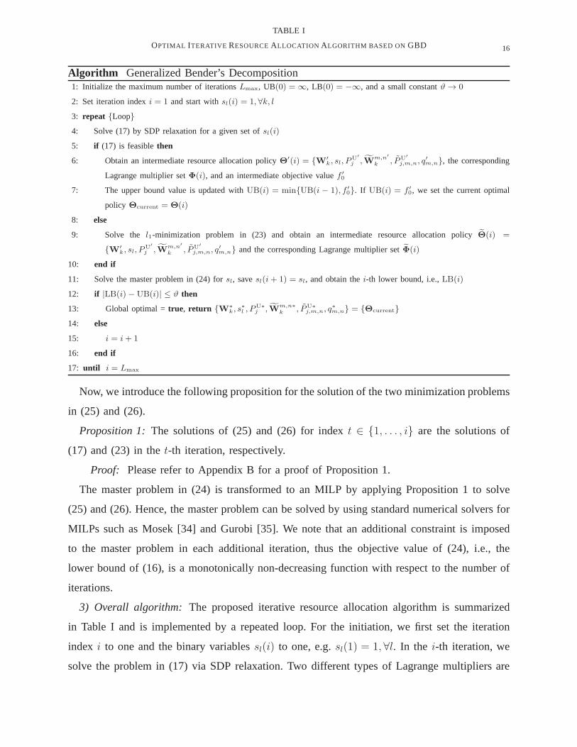
TABLE I

OPTIMAL ITERATIVE RESOURCEALLOCATION ALGORITHM BASED ON GBD

Algorithm Generalized Bender’s Decomposition1: Initialize the maximum number of iterationsLmax, UB(0) = ∞, LB(0) = −∞, and a small constantϑ → 0

2: Set iteration indexi = 1 and start withsl(i) = 1, ∀k, l

3: repeat Loop

4: Solve (17) by SDP relaxation for a given set ofsl(i)

5: if (17) is feasiblethen

6: Obtain an intermediate resource allocation policyΘ′(i) = W′

k, sl, PU′

j ,Wm,n′

k , PU′

j,m,n, q′

m,n, the corresponding

Lagrange multiplier setΦ(i), and an intermediate objective valuef ′

0

7: The upper bound value is updated withUB(i) = minUB(i − 1), f ′

0. If UB(i) = f ′

0, we set the current optimal

policy Θcurrent = Θ(i)

8: else

9: Solve the l1-minimization problem in (23) and obtain an intermediate resource allocation policyΘ(i) =

W′

k, sl, PU′

j ,Wm,n′

k , PU′

j,m,n, q′

m,n and the corresponding Lagrange multiplier setΦ(i)

10: end if

11: Solve the master problem in (24) forsl, savesl(i+ 1) = sl, and obtain thei-th lower bound, i.e.,LB(i)

12: if |LB(i)− UB(i)| ≤ ϑ then

13: Global optimal =true, return W∗

k, s∗

l , PU∗

j ,Wm,n∗

k , PU∗

j,m,n, q∗

m,n = Θcurrent

14: else

15: i = i+ 1

16: end if

17: until i = Lmax

Now, we introduce the following proposition for the solution of the two minimization problems

in (25) and (26).

Proposition 1: The solutions of (25) and (26) for indext ∈ 1, . . . , i are the solutions of

(17) and (23) in thet-th iteration, respectively.

Proof: Please refer to Appendix B for a proof of Proposition 1.

The master problem in (24) is transformed to an MILP by applying Proposition 1 to solve

(25) and (26). Hence, the master problem can be solved by using standard numerical solvers for

MILPs such as Mosek [34] and Gurobi [35]. We note that an additional constraint is imposed

to the master problem in each additional iteration, thus theobjective value of (24), i.e., the

lower bound of (16), is a monotonically non-decreasing function with respect to the number of

iterations.

3) Overall algorithm: The proposed iterative resource allocation algorithm is summarized

in Table I and is implemented by a repeated loop. For the initiation, we first set the iteration

index i to one and the binary variablessl(i) to one, e.g.sl(1) = 1, ∀l. In the i-th iteration, we

solve the problem in (17) via SDP relaxation. Two different types of Lagrange multipliers are

17

defined depending on the feasibility of the primal problem. If the problem is feasible for a given

sl(i) (lines 6, 7), then we obtain an intermediate resource allocation policyΘ(i), an intermediate

objective valuef ′0, and the corresponding Lagrange multiplier setΦ(i). In particular,Φ(i) is used

to generate anoptimality cut in the master problem. Also, the optimal resource allocation policy

and the performance upper boundUB(i) are updated if the computed objective value is the lowest

across all the iterations. On the contrary, if the primal problem is infeasible for a givensl(i)

(line 9), then we solve thel1-minimization problem in (23) and obtain an intermediate resource

allocation policyΘ(i) and the corresponding Lagrange multiplier setΦ(i). This information will

be used to generate aninfeasibility cut in the master problem. We note that the upper bound

is obtained only from the feasible primal problem. Subsequently, we solve the master problem

based onΘ(t) andΘ(i), t ∈ 1, . . . , i, via a standard MILP numerical solver. Due to weak

duality [26], the optimal value of the original optimization problem in (17) is bounded below

by the objective value of the master problem in each iteration. The algorithm stops when the

difference between thei-th lower bound and thei-th upper bound is smaller than a predefined

thresholdϑ ≥ 0 (lines 12 – 14). We note that when the master and the primal problems can be

solved in each iteration, the proposed algorithm is guaranteed to converge to the optimal solution

[25, Theorem 6.3.4].

C. Suboptimal Resource Allocation Algorithm Design

The optimal iterative resource allocation algorithm proposed in the last section has a non-

polynomial time computational complexity due to the MILP master problem4. In this section, we

propose a suboptimal resource allocation algorithm which has a polynomial time computational

complexity. The starting point for the design of the proposed suboptimal resource allocation

algorithm is the reformulated optimization problem in (13).

1) Problem reformulation via difference of convex functions programming: The major obstacle

in solving (13) are the binary constraints. Hence, we rewrite constraint C5 in its equivalent form:

C5a: 0 ≤ sl ≤ 1, ∀l ∈ 1 . . . , L and C5b:NTL∑

l=1

sl −NTL∑

l=1

s2l ≤ 0. (27)

Now, optimization variablessl in C5a are continuous values between zero and one while

constraint C5b is the difference of two convex functions. Byusing the SDP relaxation approach

4The optimal algorithm serves mainly as a performance benchmark for the proposed suboptimal algorithm.

18

TABLE II

SUBOPTIMAL ITERATIVE RESOURCEALLOCATION ALGORITHM

Algorithm Successive Convex Approximation1: Initialize the maximum number of iterationsLmax, penalty factorφ ≫ 0, iteration indexi = 0, ands(i)l

2: repeat Loop

3: Solve (31) for a givens(i+1)l and obtain the intermediate resource allocation policyW′

k, s′

l, PU′

j ,Wm,n′

k , PU′

j,m,n, q′

m,n

4: Sets(i+1)l = s′l and i = i+ 1

5: until Convergence ori = Lmax

as in the optimal resource allocation algorithm, we can reformulate the optimization problem as

minimizeWk∈H

NTL,Wlk,b

,PUj ,PU

j,m,n,qm,n

UTP

(Wk, sl, P

Uj

)(28)

s.t. Θ ∈ D, C5b,

whereD denotes the convex feasible solution set spanned by constraints C1, C2,C3, C4, C5a, C6,

and C8 – C18. The only non-convexity in (28) is due to constraint C5b which is a reverse convex

function [27]. Now, we introduce the following Theorem for handling the constraint.

Theorem 2: For a large constant valueφ≫ 1, (28) is equivalent5 to the following problem:

minimizeWk∈H

NTL,Wlk,b

,PUj ,PU

j,m,n,qm,n

UTP

(Wk, sl, P

Uj

)+ φ(NTL∑

l=1

sl −NTL∑

l=1

s2l

)(29)

s.t. Θ ∈ D.

In particular,φ acts as a large penalty factor for penalizing the objective function for anysl that

is not equal to0 or 1.

Proof: Please refer to Appendix C for a proof of Theorem 2.

The problem in (29) is in the canonical form of difference of convex (d.c.) functions pro-

gramming. Specifically,g(sl) =∑NTL

l=1 s2l is a concave function and we minimize d.c. functions

over a convex constraint set. As a result, we can apply successive convex approximation [36] to

obtain a local optimal solution of (29).

2) Suboptimal iterative algorithm: Sinceg(sl) is a differentiable convex function, inequality

g(sl) ≥ g(s(i)l ) +∇slg(s

(i)l )(sl − s

(i)l ), ∀l ∈ 1, . . . , NTL, (30)

always holds for any feasible points(i)l , where the right hand side of (30) is an affine function

[33] and represents a global underestimator ofg(sl).

5Here, equivalence means that both problems share the same optimal objective value and the same optimal resource allocation

policy.

19

As a result, for any given value ofs(i)l , we solve the following optimization problem,

minimizeWk∈H

NTL,Wlk,b

,sl,PUj ,PU

j,m,n,qm,n

UTP

(Wk, sl, P

Uj

)+ φ(NTL∑

l=1

sl−NTL∑

l=1

(s(i)l )2−2

NTL∑

l=1

s(i)l (sl−s

(i)l ))

s.t. Θ ∈ D, (31)

which leads to an upper bound of (29). Then, to tighten the obtained upper bound, we employ

an iterative algorithm which is summarized in Table II. First, we initialize the value ofs(i)l for

iteration indexi = 0. Then, in each iteration, we solve (31) for given values ofs(i)l , cf. line 3,

and updates(i+1)l with the intermediate solutions′l, cf. line 4. The proposed iterative method

generates a sequence of feasible solutionss(i+1)l with respect to (29) by solving the convex

upper bound problem (31) successively. As shown in [36], theproposed suboptimal iterative

algorithm converges to a local optimal solution6 of (29) with polynomial time computational

complexity. In fact, the proposed suboptimal algorithm benefits from the convexity of (31)

and different numerical methods can be used to efficiently solve (31). In particular, when the

primal-dual path-following interior-point method is used with a proper choice of kernel(/barrier)

function, cf. [37], [38], the computational complexity of the proposed suboptimal algorithm

is O(Lmax(NTL)2 ln((NTL)

2/ǫ)) with respect toNTL for a given solution accuracyǫ > 0

[39], whereO(·) stands for the big-O notation. The computational complexity is significantly

reduced compared to the computational complexity of an exhaustive search which is given by

O(2NTL(NTL ln(NTL/ǫ)) with respect toNTL, i.e., cf. Figure 3.

Remark 4: The proposed algorithm requiress(i)l to be a feasible point for the initialization,

i.e., for i = 0. This point can be easily obtained since the constraints in (29) span a convex set.

V. SIMULATION RESULTS

In this section, we evaluate the system performance of the proposed resource allocation designs

via simulations. There areL = 3 FD radio BSs in the system, which are placed at the corner

points of an equilateral triangle. The inter-site distancebetween any two FD radio BSs is250

meters. The uplink and downlink users are uniformly distributed inside a disc with radius500

meters centered at the centroid of the triangle. We set the constant weights for the downlink and

uplink power consumption asη = ζj = 1, ∀j ∈ 1, . . . , KU. The penalty termφ for the proposed

6By following a similar approach as in the proof of Theorem 1, it can be shown thatRank(Wk) = 1 holds despite the

adopted SDP relaxation.

20

TABLE III

SYSTEM PARAMETERS

Carrier center frequency and path loss exponent 1.9 GHz and3.6

Multipath fading distribution and total noise variance,σ2z Rayleigh fading and−62 dBm

Minimum required SINR for uplink userj, ΓULreqj

10 dB

Power amplifier power efficiency and antenna power consumption in idle mode,P Idle 1/εD = 1/εU = 0.2 and0 dBm

Max. transmit power for downlink and uplink,PDLmaxl

andPUmaxj

48 dBm and23 dBm

suboptimal algorithm is set to10PDLmaxl

. Also,P0 = 0 is adopted in all simulation results7. Unless

specified otherwise, we assume50 dB of self-interference cancellation8 at the FD radio BSs and

the circuit power consumption per antenna isPActive = 30 dBm. The antenna gains for the BSs

and the users are10 dBi and 0 dBi, respectively, and there areNT = 20 antennas equipped

in each FD BS resulting inNTL = 60 antennas in the network. Furthermore, all downlink

users require identical minimum SINRs, i.e.,ΓDLreqk

= ΓDLreq, ∀k. The performance of the proposed

algorithms is compared with the performances of the following four baseline systems designed

for peak system load when all the available antennas are activated. In particular, we minimize

the total system power consumption of all four baseline systems using a similar approach as for

the schemes proposed in this paper but setsl = 1, ∀l ∈ 1, . . . , NTL. The baseline systems are

configured as follows.Baseline 1: a FD distributed antenna system (FD-DAS);Baseline 2: a HD

distributed antenna system (HD-DAS);Baseline 3: a FD system with co-located antennas (FD-

CAS); Baseline 4: a HD system with co-located antennas (HD-CAS). For the HD communication

systems, we adopt static time division duplex such that uplink and downlink communication

occur in non-overlapping equal-length time intervals. In other words, both self-interference and

the uplink-to-downlink co-channel interference are avoided. For a fair performance comparison

between HD and FD systems, we setlog2(1+ΓULreqj

) = 1/2 log2(1+ΓUL−HDreqj

) andlog2(1+ΓDLreqj

) =

1/2 log2(1+ΓDL−HDreqj

) such that the minimum required SINRs for the uplink users,ΓUL−HDreqj

, and

downlink users,ΓDL−HDreqj

, becomeΓUL−HDreqj

= (1 + ΓULreqj

)2 − 1 andΓDL−HDreqj

= (1 + ΓDLreq)

2 − 1,

respectively, to account for the penalty due to the loss in spectral efficiency of the HD protocol.

Also, the power consumption of downlink and uplink transmission in the objective function of

the HD systems is reduced by a factor of two as at a given time either uplink or downlink

transmission is performed. For the CAS, we assume that thereis only one BS located at the

center of the system, which is equipped with the same number of antennas as all FD BSs in the

7We note that the value ofP0 does not affect the resource allocation algorithm design.

8We assume a balun analog circuit is implemented in the FD radio BSs which can cancel50 dB of self-interference [11].

The residual self-interference is handled by the beamforming matrixWk via the proposed optimization framework.

21

0 50 100 150 200 250 300 35035

40

45

50

Number of iterations

Ave

rage

tota

l sys

tem

po

wer

con

sum

ptio

n (d

Bm

)

0 10 20 30 40 50 60

46

47

48

49

Number of iteartions

Obj

ectiv

e va

lue

of

equa

tion

(29)

(dB

m)

SINR = 24 dBOptimal value, SINR = 24 dBSINR = 21 dBOptimal value, SINR = 21 dB

Upper bound, SINR = 24 dBLower bound, SINR = 24 dBUpper bound, SINR = 21 dBLower bound, SINR = 21 dB

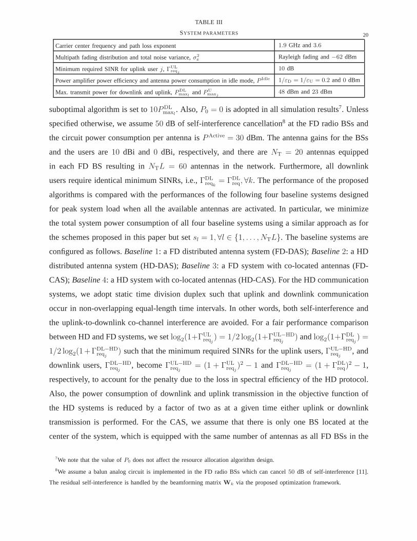
Fig. 2. Convergence of the proposed iterative algorithms.

30 40 50 60 70 80 90 10010

5

1010

1015

1020

1025

1030

1035

Number of BS antennas (NTL)

Com

puta

tiona

l com

plex

ity

Proposed suboptimal algorithmBrute force search

Computational complexityreduction

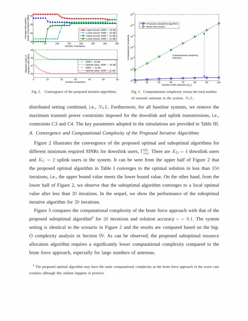
Fig. 3. Computational complexity versus the total number

of transmit antennas in the system,NTL.

distributed setting combined, i.e.,NTL. Furthermore, for all baseline systems, we remove the

maximum transmit power constraints imposed for the downlink and uplink transmissions, i.e.,

constraints C3 and C4. The key parameters adopted in the simulations are provided in Table III.

A. Convergence and Computational Complexity of the Proposed Iterative Algorithms

Figure 2 illustrates the convergence of the proposed optimal and suboptimal algorithms for

different minimum required SINRs for downlink users,ΓDLreq. There areKD = 4 downlink users

andKU = 2 uplink users in the system. It can be seen from the upper half of Figure 2 that

the proposed optimal algorithm in Table I converges to the optimal solution in less than350

iterations, i.e., the upper bound value meets the lower bound value. On the other hand, from the

lower half of Figure 2, we observe that the suboptimal algorithm converges to a local optimal

value after less than20 iterations. In the sequel, we show the performance of the suboptimal

iterative algorithm for20 iterations.

Figure 3 compares the computational complexity of the bruteforce approach with that of the

proposed suboptimal algorithm9 for 20 iterations and solution accuracyǫ = 0.1. The system

setting is identical to the scenario in Figure 2 and the results are computed based on the big-

O complexity analysis in Section IV. As can be observed, the proposed suboptimal resource

allocation algorithm requires a significantly lower computational complexity compared to the

brute force approach, especially for large numbers of antennas.

9 The proposed optimal algorithm may have the same computational complexity as the brute force approach in the worst case

scenario although this seldom happens in practice.

22

12 14 16 18 20 22 24 26 28 3040

45

50

55

60

65

70

75

80

85

Minimum required SINR of downlink users (dB)

Ave

rage

tota

l sys

tem

pow

er c

onsu

mpt

ion

(dB

m)

Optimal algorithmSuboptimal algorithmBaseline 1: FD−DASBaseline 2: HD−DASBaseline 3: FD−CASBaseline 4: HD−CAS

Performance gain

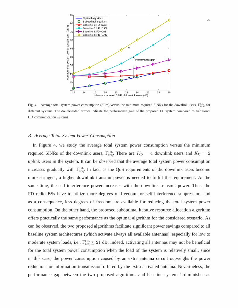
Fig. 4. Average total system power consumption (dBm) versusthe minimum required SINRs for the downlink users,ΓDLreq, for

different systems. The double-sided arrows indicate the performance gain of the proposed FD system compared to traditional

HD communication systems.

B. Average Total System Power Consumption

In Figure 4, we study the average total system power consumption versus the minimum

required SINRs of the downlink users,ΓDLreq. There areKD = 4 downlink users andKU = 2

uplink users in the system. It can be observed that the average total system power consumption

increases gradually withΓDLreq. In fact, as the QoS requirements of the downlink users become

more stringent, a higher downlink transmit power is needed to fulfill the requirement. At the

same time, the self-interference power increases with the downlink transmit power. Thus, the

FD radio BSs have to utilize more degrees of freedom for self-interference suppression, and

as a consequence, less degrees of freedom are available for reducing the total system power

consumption. On the other hand, the proposed suboptimal iterative resource allocation algorithm

offers practically the same performance as the optimal algorithm for the considered scenario. As

can be observed, the two proposed algorithms facilitate significant power savings compared to all

baseline system architectures (which activate always all available antennas), especially for low to

moderate system loads, i.e.,ΓDLreq ≤ 21 dB. Indeed, activating all antennas may not be beneficial

for the total system power consumption when the load of the system is relatively small, since

in this case, the power consumption caused by an extra antenna circuit outweighs the power

reduction for information transmission offered by the extra activated antenna. Nevertheless, the

performance gap between the two proposed algorithms and baseline system1 diminishes as

23

1 2 3 4 5

35

40

45

50

55

60

65

Number of downlink users (KD)

Ave

rage

tota

l sys

tem

pow

er c

onsu

mpt

ion

(dB

m)

Optimal algorithmSuboptimal algorithmBaseline 1: FD−DASBaseline 2: HD− DASBaseline 3: FD− CASBaseline 4: HD− CAS

Performance gain

FD systems

HD systems

Proposed algorithms

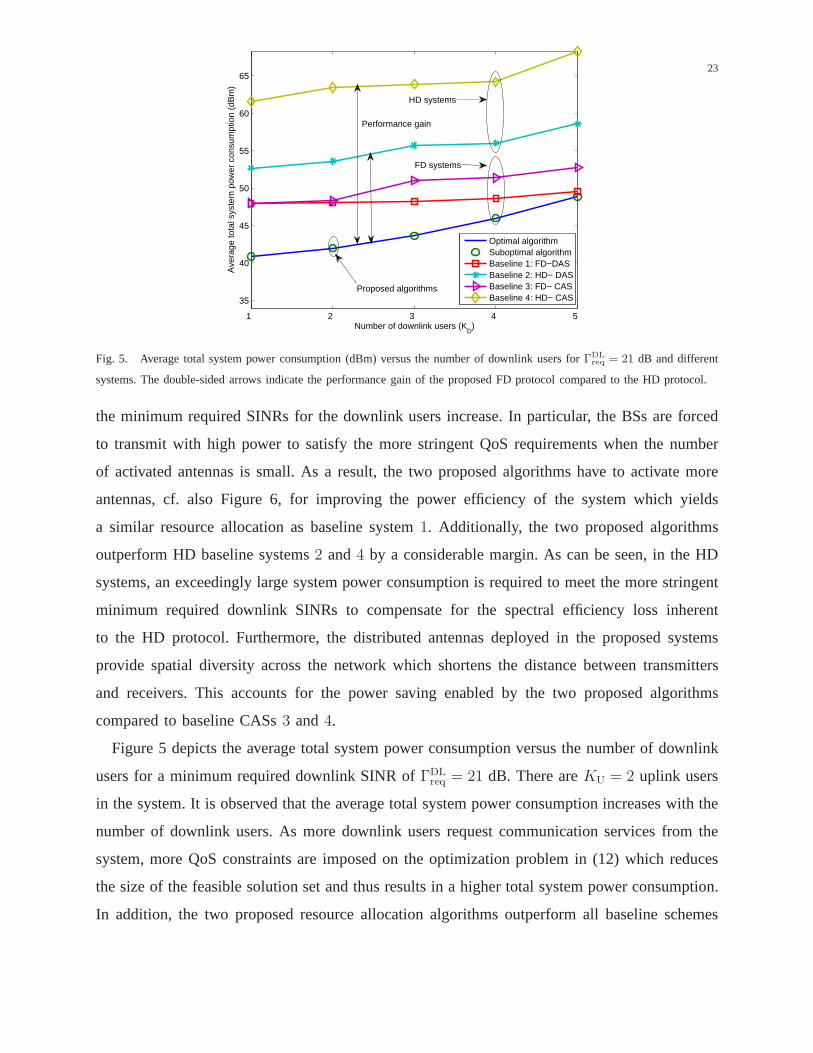
Fig. 5. Average total system power consumption (dBm) versusthe number of downlink users forΓDLreq = 21 dB and different

systems. The double-sided arrows indicate the performancegain of the proposed FD protocol compared to the HD protocol.

the minimum required SINRs for the downlink users increase.In particular, the BSs are forced

to transmit with high power to satisfy the more stringent QoSrequirements when the number

of activated antennas is small. As a result, the two proposedalgorithms have to activate more

antennas, cf. also Figure 6, for improving the power efficiency of the system which yields

a similar resource allocation as baseline system1. Additionally, the two proposed algorithms

outperform HD baseline systems2 and4 by a considerable margin. As can be seen, in the HD

systems, an exceedingly large system power consumption is required to meet the more stringent

minimum required downlink SINRs to compensate for the spectral efficiency loss inherent

to the HD protocol. Furthermore, the distributed antennas deployed in the proposed systems

provide spatial diversity across the network which shortens the distance between transmitters

and receivers. This accounts for the power saving enabled bythe two proposed algorithms

compared to baseline CASs3 and4.

Figure 5 depicts the average total system power consumptionversus the number of downlink

users for a minimum required downlink SINR ofΓDLreq = 21 dB. There areKU = 2 uplink users

in the system. It is observed that the average total system power consumption increases with the

number of downlink users. As more downlink users request communication services from the

system, more QoS constraints are imposed on the optimization problem in (12) which reduces

the size of the feasible solution set and thus results in a higher total system power consumption.

In addition, the two proposed resource allocation algorithms outperform all baseline schemes

24

12 14 16 18 20 22 24 26 28 305

10

15

20

25

30

Minimum required SINR of downlink users (dB)

Ave

rage

num

ber

of a

ctiv

ated

ant

enna

s (N

TL)

Optimal algorithm, KD = 4

Suboptimal algorithm, KD = 4

Optimal algorithm, KD = 3

Suboptimal algorithm, KD = 3

Optimal algorithm, KD = 2

Suboptimal algorithm, KD = 2

Optimal algorithm, KD = 1

Suboptimal algorithm, KD = 1

KD = 1

KD = 4

KD = 3

KD = 2

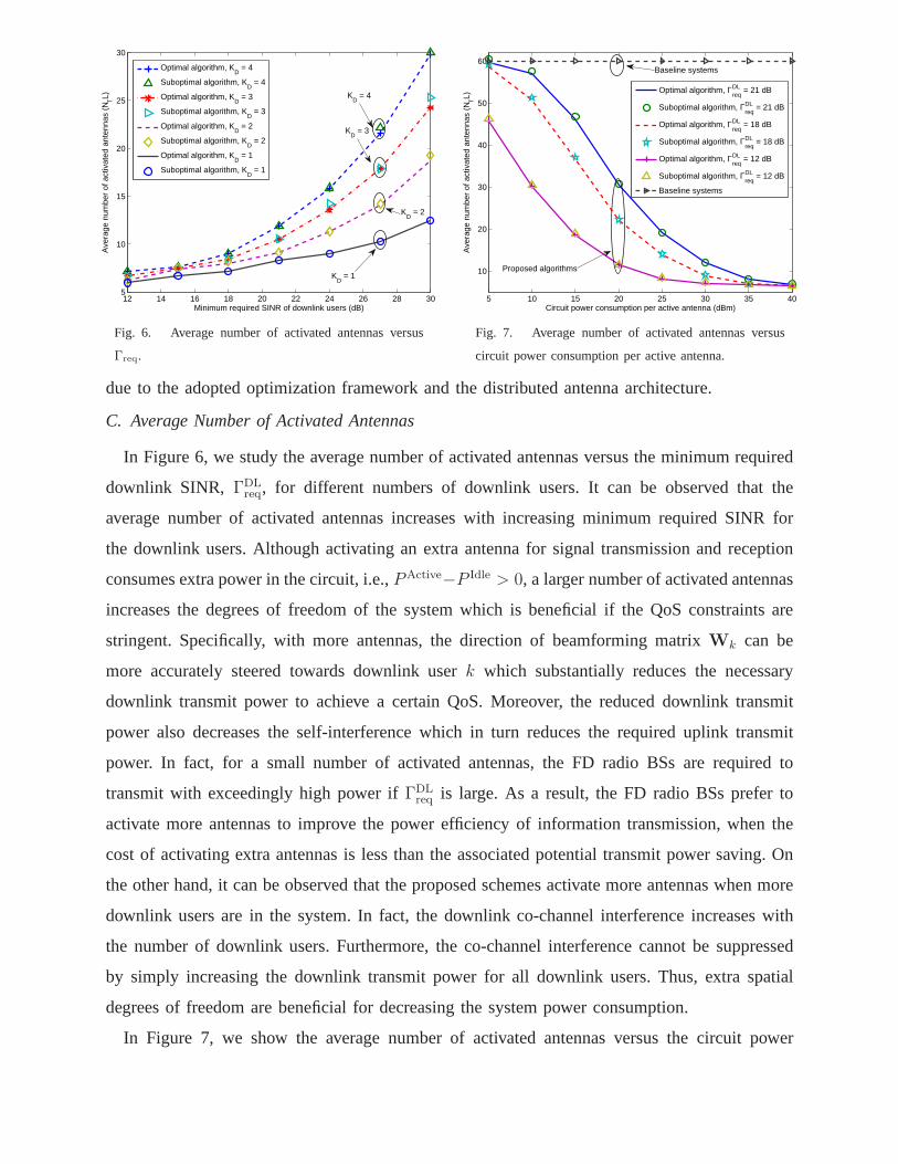
Fig. 6. Average number of activated antennas versus

Γreq.

5 10 15 20 25 30 35 40

10

20

30

40

50

60

Circuit power consumption per active antenna (dBm)

Ave

rage

num

ber

of a

ctiv

ated

ant

enna

s (N

TL)

Optimal algorithm, ΓDLreq

= 21 dB

Suboptimal algorithm, ΓDLreq

= 21 dB

Optimal algorithm, ΓDLreq

= 18 dB

Suboptimal algorithm, ΓDLreq

= 18 dB

Optimal algorithm, ΓDLreq

= 12 dB

Suboptimal algorithm, ΓDLreq

= 12 dB

Baseline systems

Proposed algorithms

Baseline systems

Fig. 7. Average number of activated antennas versus

circuit power consumption per active antenna.

due to the adopted optimization framework and the distributed antenna architecture.

C. Average Number of Activated Antennas

In Figure 6, we study the average number of activated antennas versus the minimum required

downlink SINR, ΓDLreq, for different numbers of downlink users. It can be observedthat the

average number of activated antennas increases with increasing minimum required SINR for

the downlink users. Although activating an extra antenna for signal transmission and reception

consumes extra power in the circuit, i.e.,PActive−P Idle > 0, a larger number of activated antennas

increases the degrees of freedom of the system which is beneficial if the QoS constraints are

stringent. Specifically, with more antennas, the directionof beamforming matrixWk can be

more accurately steered towards downlink userk which substantially reduces the necessary

downlink transmit power to achieve a certain QoS. Moreover,the reduced downlink transmit

power also decreases the self-interference which in turn reduces the required uplink transmit

power. In fact, for a small number of activated antennas, theFD radio BSs are required to

transmit with exceedingly high power ifΓDLreq is large. As a result, the FD radio BSs prefer to

activate more antennas to improve the power efficiency of information transmission, when the

cost of activating extra antennas is less than the associated potential transmit power saving. On

the other hand, it can be observed that the proposed schemes activate more antennas when more

downlink users are in the system. In fact, the downlink co-channel interference increases with

the number of downlink users. Furthermore, the co-channel interference cannot be suppressed

by simply increasing the downlink transmit power for all downlink users. Thus, extra spatial

degrees of freedom are beneficial for decreasing the system power consumption.

In Figure 7, we show the average number of activated antennasversus the circuit power

25

consumption per active antenna,PActive (dBm), for different minimum required SINRs for the

downlink users. It is expected that the FD radio BSs prefer toactivate more antennas when

the circuit power consumption per antenna is small or the SINR requirements of the downlink

users are demanding, since in this case, the power savings achieved by activating extra antennas

surpasses the corresponding circuit power consumption. Onthe contrary, when the circuit power

consumption per antenna is high, the FD radio BSs become moreconservative in activating

antennas since using a large number of antennas may no longerbe beneficial to the overall

system power consumption.

VI. CONCLUSIONS

In this paper, we formulated the resource allocation algorithm design for power efficient

distributed FD antenna networks as a mixed combinatorial and non-convex optimization problem,

where the antenna circuit power consumption and the QoS requirements of the uplink and

downlink users were taken into account. Applying the generalized Bender’s decomposition, we

developed an optimal iterative resource allocation algorithm for solving the problem optimally. In

addition, a polynomial time computational complexity suboptimal algorithm was also proposed

to strike a balance between computational complexity and optimality. Simulation results showed

that the proposed suboptimal iterative resource allocation algorithm approaches the optimal

performance in a small number of iterations. Furthermore, our results unveiled the substantial

power savings enabled in FD radio distributed antennas networks by dynamically switching off

a subset of the available antennas; an exceedingly large number of activated antennas may not

be a cost effective solution for reducing the total system power consumption when the QoS

requirements of the users are not stringent.

APPENDIX

A. Proof of Theorem 1

We start the proof by rewriting the Lagrangian function of the primal problem in (17) in terms

of the beamforming matrixWk:

L(Θ,Φ

)=

KD∑

k=1

Tr(AkWk)−KD∑

k=1

Tr((

Zk +αkHDk

ΓDLreqk

)Wk

)+∆ (32)

and Ak = ηεDINTL+

KD∑

j 6=k

αjHDj+

NTL∑

l=1

ρRl +

NTL∑

m=1

NTL∑

n=1

(DC17k,m,n

−DC16k,m,n

). (33)

26

∆ denotes the collection of variables that are independent ofWk. For convenience, the optimal

primal and dual variables of the SDP relaxed version of (17) are denoted by the corresponding

variables with an asterisk superscript. By exploiting the Karush-Kuhn-Tucker (KKT) optimality

conditions, we obtain the following equations:

Z∗k0, α∗

k ≥ 0, ∀k, (34)

Z∗kW

∗k=0, (35)

Z∗k=A∗

k −α∗kHDk

ΓDLreqk

, (36)

whereA∗k in (36) is obtained by substituting the optimal dual variablesΦ∗ into (33). From (35),

we know that the optimal beamforming matrixW∗k is a rank-one matrix whenRank(Z∗

k) =

NTL − 1. In particular,W∗k is required to lie in the null space spanned byZ∗

k for W∗k 6= 0.

As a result, by revealing the structure ofZ∗k, we can study the rank of beamforming matrix

W∗k. In the following, we first show by contradiction thatA∗

k is a positive definite matrix with

probability one. To this end, we focus on the dual problem in (22). For a given set of optimal

dual variables,Φ∗, and a subset of optimal primal variables,s∗l , PU∗j ,Wm,n∗

k , PU∗j,m,n, q

∗m,n, the

dual problem in (22) can be written as

minimizeWk∈H

NT

L(Θ,Φ∗

). (37)

SupposeA∗k is negative semi-definite, i.e.,A∗

k 0, then we can construct a beamforming

matrix Wk = rwkwHk as one of the solutions of (37), wherer > 0 is a scaling parameter and

wk is the eigenvector corresponding to one of the non-positiveeigenvalues ofA∗k. We substitute

Wk = rwkwHk into (37) which yields

L(Θ,Φ

)=

KD∑

k=1

Tr(rA∗kwkw

Hk )

︸ ︷︷ ︸≤0

−rKD∑

k=1

Tr(wkw

Hk

(Z∗

k +α∗kHDk

ΓDLreqk

))+∆. (38)

Besides, constraint C1 is satisfied with equality for the optimal solution and thusαk > 0.

Furthermore, since the channel vectors of the downlink users, i.e.,hDk, ∀k ∈ 1, . . . , KD, are

assumed to be statistically independent, we obtain−r∑KD

k=1Tr(wkw

Hk

(Z∗

k +α∗

kHDk

ΓDLreqk

))→ −∞

when we setr → ∞. Thus, the dual optimal value becomes unbounded from below.Yet, the

optimal value of the primal problem in (17) is non-negative for ΓDLreqk

> 0 which leads to

a contradiction as strong duality does not hold. Therefore,for the optimal solution,A∗k is a

positive definite matrix with probability one andRank(A∗k) = NTL, i.e.,A∗

k has full rank.

27

Then, by exploiting (36) and basic rank inequality results,we have the following implication:

Rank(Z∗k) + Rank

(α∗k

HDk

ΓDLreqk

)≥ Rank

(Z∗

k + α∗k

HDk

ΓDLreqk

)= Rank(A∗

k) = NTL

⇒ Rank(Z∗k) ≥ NTL− 1. (39)

Furthermore,W∗k 6= 0 is required to satisfy C1 forΓDL

reqk> 0. Thus,Rank(Z∗

k) = NTL− 1 and

Rank(W∗k) = 1 hold with probability one.

B. Proof of Proposition 1

We start the proof by studying the solution of the SDP relaxedversion of (17) via its dual

problem in (22). For a given set of optimal dual variablesΦ(i), we haveΘ(i)

= argminΘ

UTP

(Wk, sl, P

Uj

)+f1(Θ,Φ(i))

+

KD∑

k=1

NTL∑

l=1

ρl Tr(WkRl) +

NTL∑

m=1

NTL∑

n=1

κm,nqm,n + ϕm,nqm,n − ωm,nqm,n, (40)

where the first equality is due to the KKT conditions of the SDPrelaxed version of (17). On

the other hand, we can rewrite functionξ(Φ(t), sl,k), t ∈ 1, . . . , i, in (25) asξ(Φ(t), sl,k)

=

minimize

Θ

UTP

(Wk, sl, P

Uj

)+f1(Θ,Φ(i))+

KD∑

k=1

NTL∑

l=1

ρl Tr(WkRl)+

NTL∑

m=1

NTL∑

n=1

κm,nqm,n

+ϕm,nqm,n − ωm,nqm,n

+

NTL∑

m=1

NTL∑

n=1

ωm,n(sn + sm − 1)− κm,nsm − ϕm,nsn

−KD∑

k=1

NTL∑

l=1

slPDLmaxl

(41)

The difference between (40) and (41) is a constant offset. Thus,Θ(t) is also the solution for the

minimization in the master problem in (41) for thet-th constraint in (24c). The same approach

can be adopted to prove that the solution of (23) is also the solution of (26).

C. Proof of Theorem 2

We start the proof of Theorem 2 by using theabstract Lagrangian duality [27], [40], [41]. In

particular, the optimization problem in (28) can be writtenas

minimizeΘ∈D

maximizeφ≥0

L(Θ, φ) (42)

28

where

L(Θ, φ) = UTP

(Wk, sl, P

Uj

)+ φ(NTL∑

l=1

sl −NTL∑

l=1

s2l

)(43)

and the dual problem of (28) is given by

maximizeφ≥0

minimizeΘ∈D

L(Θ, φ). (44)

For notational simplicity, we define

Ω(φ) = minimizeΘ∈D

L(Θ, φ). (45)

Then, we have the following inequalities:

maximizeφ≥0

Ω(φ) = maximizeφ≥0

minimizeΘ∈D

L(Θ, φ) (46a)

(a)≤ minimize

Θ∈Dmaximize

φ≥0L(Θ, φ) = (28), (46b)

where (a) is due to the weak duality [33]. We note that∑NTL

l=1 sl−∑NTL

l=1 s2l ≥ 0 for Θ ∈ D such

thatL(Θ, φ) is a monotonically increasing function inφ. In other words,Ω(φ) is increasing in

φ and is bounded from above by the optimal value of (42). Suppose the optimal solution for

(46a) is denoted asφ∗0 andΘ∗ = Wk, sl, P

Uj ,W

lk,b, P

Uj,m,n, qm,n, where0 ≤ φ∗

0 ≤ ∞. Then,

we study the following two cases for the solution structure of (46a). In the first case, we assume∑NTL

l=1 sl−∑NTL

l=1 s2l = 0 for (46a). As a result,Θ∗ is also a feasible solution to (28). Subsequently,

we substituteΘ∗ into the optimization problem in (28) which yields:

Ω(φ∗0) = UTP

(Wk, sl, P

Uj

)≥ (28). (47)

By utilizing (46a) and (47), we can conclude that

minimizeΘ∈D

maximizeφ≥0

L(Θ, φ) = maximizeφ≥0

minimizeΘ∈D

L(Θ, φ) (48)

must hold for∑NTL

l=1 sl −∑NTL

l=1 s2l = 0. Furthermore, the monotonicity ofΩ(φ) with respect to

φ implies thatΩ(φ) = (28), ∀φ ≥ φ∗

0, (49)

and the result of Theorem 2 follows immediately.

Now, we study the case of∑NTL

l=1 sl −∑NTL

l=1 s2l > 0 at the optimal solution for (46a). The

optimization problemmaximizeφ≥0

Ω(φ) → ∞ is unbounded from above due to the monotonicity

of functionΩ(φ) with respect toφ. This contradicts the inequality in (46a) as (28) is finite and

positive. Thus, for the optimal solution,∑NTL

l=1 sl−∑NTL

l=1 s2l = 0 holds and the result of Theorem

2 follows immediately from the first considered case.

29

REFERENCES

[1] D. Tse and P. Viswanath,Fundamentals of Wireless Communication, 1st ed. Cambridge University Press, 2005.

[2] F. Zhuang and V. Lau, “Backhaul Limited Asymmetric Cooperation for MIMO Cellular Networks via Semidefinite

Relaxation,”IEEE Trans. Signal Process., vol. 62, pp. 684–693, Feb. 2014.

[3] T. Marzetta, “Noncooperative Cellular Wireless with Unlimited Numbers of Base Station Antennas,”IEEE Trans. Wireless

Commun., vol. 9, pp. 3590–3600, Nov. 2010.

[4] D. W. K. Ng, E. Lo, and R. Schober, “Energy-Efficient Resource Allocation in OFDMA Systems with Large Numbers of

Base Station Antennas,”IEEE Trans. Wireless Commun., vol. 11, pp. 3292 –3304, Sep. 2012.

[5] R. Heath, S. Peters, Y. Wang, and J. Zhang, “A Current Perspective on Distributed Antenna Systems for the Downlink of

Cellular Systems,”IEEE Commun. Mag., vol. 51, pp. 161–167, Apr. 2013.

[6] J. Joung and S. Sun, “Energy Efficient Power Control for Distributed Transmitters with ZF-based Multiuser MIMO

Precoding,”IEEE Commun. Lett., vol. 17, pp. 1766–1769, Sep. 2013.

[7] D. Lee, H. Seo, B. Clerckx, E. Hardouin, D. Mazzarese, S. Nagata, and K. Sayana, “Transmission and Reception in

LTE-Advanced: Deployment Scenarios and Operational Challenges,”IEEE Commun. Mag., vol. 50, pp. 148–155, Feb.

2012.

[8] B. Yu, S. Mukherjee, H. Ishii, and L. Yang, “Dynamic TDD Support in the LTE-B Enhanced Local Area Architecture,”

in Proc. IEEE Global Telecommun. Conf., Dec. 2012, pp. 585–591.

[9] S. Song, Y. Chang, H. Xu, D. Zheng, and D. Yang, “Energy Efficiency Model Based on Stochastic Geometry in Dynamic

TDD Cellular Networks,” inProc. IEEE Intern. Commun. Conf., Jun. 2014, pp. 889–894.

[10] J. I. Choi, M. Jain, K. Srinivasan, P. Levis, and S. Katti, “Achieving Single Channel, Full Duplex Wireless Communication,”

in Proc. of the Sixteenth Annual Intern. Conf. on Mobile Computing and Netw., 2010, pp. 1–12.

[11] M. Jain, J. I. Choi, T. Kim, D. Bharadia, S. Seth, K. Srinivasan, P. L. S. Katti, and P. Sinha, “Practical, Real-Time,

Full Duplex Wireless,” inProc. of the Seventeenth Annual Intern. Conf. on Mobile Computing and Netw., Sep. 2011, pp.

301–312.

[12] D. Bharadia and S. Katti, “Full Duplex MIMO Radios,” inProc. 11-th USENIX Symposium on Networked Sys. Design

and Implementation, Apr. 2014.

[13] M. Duarte and A. Sabharwal, “Full-Duplex Wireless Communications using Off-the-Shelf Radios: Feasibility and First

Results,” in2010 Conference Record of the Forty Fourth Asilomar Conf. on Signals, Systems and Comput., Nov. 2010,

pp. 1558–1562.

[14] M. Duarte, C. Dick, and A. Sabharwal, “Experiment-Driven Characterization of Full-Duplex Wireless Systems,”IEEE

Trans. Wireless Commun., vol. 11, pp. 4296–4307, Dec. 2012.

[15] A. K. Khandani, “Full Duplex Wireless Transmission with Self-Interference Cancellation,” Patent US20 130 301 487A1,

2013. [Online]. Available: http://www.patentlens.net/patentlens/patent/US7062320/

[16] “Full Duplex Configuration of Un and Uu Subframes for Type I Relay,” 3GPP TSG RAN WG1 R1-100139, Tech. Rep.,

Jan 2010.

[17] “Text Proposal on Inband Full Duplex Relay for TR 36.814,” 3GPP TSG RAN WG1 R1-101659, Tech. Rep., Feb 2010.

[18] “Full-Duplex Radios for Local Access,” European Commission - Research: The Seventh Framework Programme, Tech.

Rep. [Online]. Available: http://www.fp7-duplo.eu/index.php/general-info

[19] T. Riihonen, S. Werner, and R. Wichman, “Mitigation of Loopback Self-Interference in Full-Duplex MIMO Relays,”IEEE

Trans. Signal Process., vol. 59, pp. 5983–5993, Dec. 2011.

30

[20] H. Suraweera, I. Krikidis, G. Zheng, C. Yuen, and P. Smith, “Low-Complexity End-to-End Performance Optimization in

MIMO Full-Duplex Relay Systems,”IEEE Trans. Wireless Commun., vol. 13, pp. 913–927, Feb. 2014.

[21] D. W. K. Ng, E. S. Lo, and R. Schober, “Dynamic Resource Allocation in MIMO-OFDMA Systems with Full-Duplex

and Hybrid Relaying,”IEEE Trans. Commun., vol. 60, pp. 1291–1304, May 2012.

[22] D. Nguyen, L.-N. Tran, P. Pirinen, and M. Latva-Aho, “Onthe Spectral Efficiency of Full-Duplex Small Cell Wireless

Systems,”IEEE Trans. Wireless Commun., vol. 13, pp. 4896–4910, Sep. 2014.

[23] H. Q. Ngo, H. Suraweera, M. Matthaiou, and E. Larsson, “Multipair Full-Duplex Relaying With Massive Arrays and

Linear Processing,”IEEE J. Select. Areas Commun., vol. 32, pp. 1721–1737, Sep. 2014.

[24] R. Ramamonjison, A. Haghnegahdar, and V. Bhargava, “Joint Optimization of Clustering and Cooperative Beamforming

in Green Cognitive Wireless Networks,”IEEE Trans. Wireless Commun., vol. 13, pp. 982–997, Feb. 2014.

[25] C. A. Floudas,Nonlinear and Mixed-Integer Optimization: Fundamentals and Applications, 1st ed. Oxford University

Press, 1995.

[26] D. Li and X. Sun,Nonlinear Integer Programming. Springer, 2006.

[27] E. Che, H. Tuan, and H. Nguyen, “Joint Optimization of Cooperative Beamforming and Relay Assignment in Multi-User

Wireless Relay Networks,”IEEE Trans. Wireless Commun., vol. 13, pp. 5481–5495, Oct. 2014.

[28] D. W. K. Ng and R. Schober, “Secure and Green SWIPT in Distributed Antenna Networks with Limited Backhaul

Capacity,”submitted for possible journal publication, 2014. [Online]. Available: http://arxiv.org/abs/1410.3065

[29] Y. Cheng, M. Pesavento, and A. Philipp, “Joint Network Optimization and Downlink Beamforming for CoMP Transmissions

Using Mixed Integer Conic Programming,”IEEE Trans. Signal Process., vol. 61, pp. 3972–3987, Aug. 2013.

[30] J. Lee and S. L. (Eds.),Mixed Integer Nonlinear Programming. The IMA Volumes in Mathematics and its Applications,

2012, vol. 154.

[31] W. Yu and T. Lan, “Transmitter Optimization for the Multi-Antenna Downlink With Per-Antenna Power Constraints,”

IEEE Trans. Signal Process., vol. 55, pp. 2646–2660, Jun. 2007.

[32] S. Luo, R. Zhang, and T. J. Lim, “Downlink and Uplink Energy Minimization Through User Association and Beamforming

in Cloud RAN,” submitted for possible journal publication, 2014. [Online]. Available: http://arxiv.org/abs/1402.4238

[33] S. Boyd and L. Vandenberghe,Convex Optimization. Cambridge University Press, 2004.

[34] “MOSEK ApS: Software for Large-Scale Mathematical Optimization Problems, Version 7.0.0.111,” Apr. 2014. [Online].

Available: http://www.mosek.com/

[35] “GUROBI Optimization, State-of-the-Art Mathematical Programming Solver, v5.6,” Apr. 2014. [Online]. Available:

http://www.gurobi.com/

[36] Q. T. Dinh and M. Diehl, “Local Convergence of Sequential Convex Programming for Nonlinear Programming,” inChapter

of Recent Advances in Optimization and Its Application in Engineering. Oxford University Press, 2010.

[37] B. Choi and G. Lee, “New Complexity Analysis for Primal-Dual Interior-Point Methods for Self-Scaled Optimization

Problems,”Fixed Point Theory and Applications, no. 1, p. 213, Dec. 2012.

[38] G. Wang and Y. Bai, “A New Primal-Dual Path-Following Interior-Point Algorithm for Semidefinite Optimization,”Journal

of Mathematical Analysis and Applications, vol. 353, pp. 339 – 349, 2009.

[39] I. Polik and T. Terlaky, “Interior Point Methods for Nonlinear Optimization,” inNonlinear Optimization, 1st ed., G. D.

Pillo and F. Schoen, Eds. Springer, 2010, ch. 4.

[40] C. Goh and X. Q. Yang,Duality in Optimization and Variational Inequalities, 1st ed. Taylor & Francis, 2002.

[41] R. Rockafellar,Conjugate Duality and Optimization. Society for Industrial and Applied Mathematics, 1974.