POWER CONTROL BY GEOMETRIC PROGRAMMING

MUNG CHIANG ∗, CHEE WEI TAN †, DANIEL P. PALOMAR ‡,

DANIEL O’NEILL, §DAVID JULIAN¶

Abstract. In wireless cellular or ad hoc networks where qualities of service are interference-limited, a variety of power control problems can be formulated as nonlinear optimization with asystem-wide objective, e.g., maximizing total system throughput or achieving maxmin fairness, andmany QoS constraints from individual users, e.g., on data rate, delay, and outage probability. Weshow that in the high SIR regime, these nonlinear and apparently difficult, nonconvex optimizationproblems can be transformed into convex optimization problems through geometric programming,thus can be very efficiently solved for global optimality even in large networks. In the mediumto low SIR regime, these constrained nonlinear optimization of power control cannot be turned intotractable convex formulations, but a heuristic can be used to compute the optimal solution by solvinga series of geometric programs. While efficient and robust algorithms have been extensively studiedfor centralized solutions of geometric programs, distributed algorithms have not been fully explored.We present a systematic method of distributed algorithms for power control based on geometricprograms. These techniques for power control, together with their implications to admission controland pricing in wireless networks, are illustrated through several numerical examples.

1. Introduction. Due to the broadcast nature of radio transmission, data ratesand other qualities of service in a wireless network are affected by interference. This isparticularly important in CDMA systems where users transmit at the same time overthe same frequency bands and their spreading codes are not perfectly orthogonal.Transmit power control is often used to tackle this problem of signal interference.In this chapter, we study how to optimize over the transmit powers to create theoptimal set of Signal-to-Interference Ratios (SIR) on wireless links. Optimality heremay be referring to maximizing a system-wide efficiency metric (e.g., the total systemthroughput), or maximizing a Quality of Service (QoS) metric for a user in the highestQoS class, or maximizing a QoS metric for the user with the minimum QoS metricvalue (i.e., a maxmin optimization).

While the objective represents a system-wide goal to be optimized, individualusers’ QoS requirements also need to be satisfied. Any power allocation must thereforebe constrained by a feasible set formed by these minimum requirements from theusers. Such a constrained optimization captures the tradeoff between user-centricconstraints and some network-centric objective. Because a higher power level fromone transmitter increases the interference levels at other receivers, there may not beany feasible power allocation to satisfy the requirements from all the users. Sometimesan existing set of requirements can be satisfied, but when a new user is admitted intothe system, there exists no more feasible power control solutions, or the maximizedobjective is reduced due to the tightening of the constraint set, leading to the needfor admission control and admission pricing, respectively.

Because many QoS metrics are nonlinear functions of SIR, which is in turn anonlinear (and neither convex nor concave) function of transmit powers, the abovepower control optimization or feasibility problems are difficult nonlinear optimizationproblems that may appear to be not efficiently solvable. This chapter shows that,when SIR is much larger than 0dB, a class of nonlinear optimization called Geometric

∗ELECTRICAL ENGINEERING DEPARTMENT, PRINCETON UNIVERSITY†ELECTRICAL ENGINEERING DEPARTMENT, PRINCETON UNIVERSITY‡ELECTRICAL ENGINEERING DEPARTMENT, PRINCETON UNIVERSITY§ELECTRICAL ENGINEERING DEPARTMENT, STANFORD UNIVERSITY¶QUALCOMM

1

Programming (GP) can be used to efficiently compute the globally optimal powercontrol in many of these problems, and efficiently determine the feasibility of userrequirements by returning either a feasible (and indeed optimal) set of powers or acertificate of infeasibility. This leads to an effective admission control and admissionpricing method. The key observation is that despite the apparent nonconvexity, theGP technique turns these constrained optimization of power control into nonlinearyet still convex optimization, which is intrinsically tractable despite its nonlinearityin objective and constraints. When SIR is comparable to or below 0dB, the powercontrol problems are truly nonconvex with no efficient and global solution methods. Inthis case, we present a heuristic that empirically almost always compute the globallyoptimal power allocation by solving a sequence of GPs.

The GP approach reveals the hidden convexity structure, thus efficient solutionmethods, in power control problems with nonlinear objective functions, and clearlydifferentiates the tractable formulations in high-SIR regime from the intractable onesin low-SIR regime. Power control by GP is applicable to formulations in both cellularnetworks with single-hop transmission between mobile users and base stations andad hoc networks with mulithop transmission among the nodes, as illustrated throughseveral numerical examples in this chapter. Traditionally, GP is solved by centralizedcomputation through the highly efficient interior point methods. We also outline anew result on how GP can be solved distributively with message passing.

The rest of this chapter is organized as follows. In section 2, we provide a con-cise introduction to GP. Section 3 is the core section of this chapter, with severalsubsections each discussing GP based power control with different representative for-mulations in cellular and multihop networks, with centralized computation and forhigh-SIR regime. This section’s results are based on an Infocom 2002 paper [14]. Twopreviously unpublished extensions are then presented: solution method for low-SIRregime in section 4 and distributed algorithm in section 5.

2. Geometric Programming. GP is a class of nonlinear, nonconvex optimiza-tion with many useful theoretical and computational properties. Since a GP canbe turned into a convex optimization problem 1, a local optimum is also a globaloptimum, duality gap is zero under mild conditions, and a global optimum can becomputed very efficiently. Numerical efficiency holds both in theory and in practice:interior point methods applied to GP have provably polynomial time complexity [18],and are very fast in practice (see, e.g., the algorithms and discussions on numericalefficiency in [16]) with high-quality software downloadable from the Internet (e.g., theMOSEK package). Convexity and duality properties of GP are well understood, andlarge-scale, robust numerical solvers for GP are available. Furthermore, special struc-tures in GP and its Lagrange dual problem lead to distributed algorithms, physicalinterpretations, and computational acceleration beyond the generic results for convexoptimization.

GP was invented in 1960s [12] and applied to primarily mechanical and chemi-cal engineering problems in 1960s and 1970s and then to several other science andengineering disciplines [1, 3, 4, 5]. Since mid-1990s, GP has been used to solve avariety of analysis and design problems in communication systems, including recentlyto wireless network power control [14, 15], resource allocation [9], joint congestioncontrol and power control [6], queuing systems [10], information theory [8], as well as

1Minimizing a convex objective function subject to upper bound inequality constraints on convexconstraint functions and linear equality constraints is a convex optimization problem.

2

to coding and signal processing. A detailed tutorial of GP and comprehensive surveyof its recent applications to communication systems can be found in [7]. This sectioncontains a brief introduction of GP terminology for applications to be shown in thenext three sections.

2.1. Basic formulations. There are two equivalent forms of GP: standard formand convex form. The first is a constrained optimization of a type of function calledposynomial, and the second form is obtained from the first through logarithmic changeof variable. 2

We first define a monomial as a function f : Rn++ → R:

f(x) = dxa(1)

1 xa(2)

2 . . . xa(n)

n

where the multiplicative constant d ≥ 0 and the exponential constants a(j) ∈ R, j =1, 2, . . . , n. A sum of monomials, indexed by k below, is called a posynomial:

f(x) =K

∑

k=1

dkxa(1)

k

1 xa(2)

k

2 . . . xa(n)

kn .

where dk ≥ 0, k = 1, 2, . . . , K, and a(j)k ∈ R, j = 1, 2, . . . , n, k = 1, 2, . . . , K. The key

features about posynomial are its positivity and convexity (in log domain).For example, 2x−π

1 x0.52 +3x1x

1003 is a posynomial in x, x1−x2 is not a posynomial,

and x1/x2 is a monomial, thus also a posynomial.Minimizing a posynomial subject to posynomial upper bound inequality con-

straints and monomial equality constraints is called GP in standard form:

minimize f0(x)subject to fi(x) ≤ 1, i = 1, 2, . . . , m,

hl(x) = 1, l = 1, 2, . . . , M(2.1)

where fi, i = 0, 1, . . . , m, are posynomials: fi(x) =∑Ki

k=1 dikxa(1)

ik

1 xa(2)

ik

2 . . . xa(n)

ikn , and

hl, l = 1, 2, . . . , M are monomials: hl(x) = dlxa(1)

l

1 xa(2)

l

2 . . . xa(n)

ln . 3

GP in standard form is not a convex optimization problem, because posynomialsare not convex functions. However, with a logarithmic change of the variables andmultiplicative constants: yi = log xi, bik = log dik , bl = log dl, and a logarithmicchange of the functions’ values, we can turn it into the following equivalent problem4 in y:

minimize p0(y) = log∑K0

k=1 exp(aT0ky + b0k)

subject to pi(y) = log∑Ki

k=1 exp(aTiky + bik) ≤ 0, i = 1, 2, . . . , m,

ql(y) = aTl y + bl = 0, l = 1, 2, . . . , M.

(2.2)

2Standard form GP is often used in network resource allocation problems, and convex form GPin problems based on stochastic models such as information theoretic problems.

3Note that a monomial equality constraint can also be expressed as two monomial inequalityconstraints: hl(x) ≥ 1 and hl(x) ≤ 1. Thus a standard form GP can be defined as the minimizationof a posynomial under upper bound inequality constraints on posynomials.

4Equivalence relationship between two optimization problems is used in a loose way here. If theoptimized value of problem A is a simple (e.g., monotonic and invertible) function of the optimizedvalue of problem B, and an optimizer of problem B can be easily computed from an optimizer ofproblem A (e.g., through a simple mapping), then problems A and B are said to be equivalent.

3

This is referred to as GP in convex form, which is a convex optimization problemsince it can be verified that the log-sum-exp function is convex [5].

In summary, GP is a nonlinear, nonconvex optimization problem that can betransformed into a nonlinear, convex problem. Therefore, a local optimum for GP isalso a global optimum, and the duality gap is zero under mild technical conditions.

2.2. Duality, feasibility, and sensitivity analysis. The Lagrange dual prob-lem of GP has interesting structures. In particular, dual GP is linearly constrainedand its objective function is a generalized entropy function [12]. Following the stan-dard procedure of deriving the Lagrange dual problem [5], it is readily verified thatfor the following GP over y with m posynomial constraints,

minimize log∑K0

k=1 exp(aT0ky + b0k)

subject to log∑Ki

k=1 exp(aTiky + bik) ≤ 0, i = 1, . . . , m,

the Lagrange dual problem is

maximize bT0 ν0 −

∑K0

j=1 ν0j log ν0j +∑m

i=1

(

bTi νi −

∑Ki

j=1 νij logνij

1T νi

)

subject to νi � 0, i = 0, . . . , m,

1Tν0 = 1,

∑mi=0 AT

i νi = 0

(2.3)

where the optimization variables are (m+1) vectors: ν i, i = 0, 1, . . . , m. The lengthof νi is Ki, i.e., the number of monomial terms in the ith posynomial, i = 0, 1, . . . , m.Here, A0 is the matrix of the exponential constants in the objective function, whereeach row corresponds to each monomial term (i.e., aT

0k is the kth row in matrixA0), and Ai, i = 1, 2, . . . , m, are the matrices of the exponential constants in theconstraint functions, again with each row corresponding to each monomial term. Themultiplicative constants in the objective function are denoted as b0 and those in theith constraint as bi, i = 1, 2, . . . , m. Linearity of dual problem constraints is utilizedin some very efficient GP solvers (e.g., [16]) that solve both the primal and dualproblems of a GP simultaneously.

Testing whether there is any variable x that satisfies a set of posynomial inequalityand monomial equality constraints:

fi(x) ≤ 1, i = 1, . . . , m, hl(x) = 1, l = 1, . . . , M(2.4)

is called a GP feasibility problem. Solving feasibility problem is useful when we wouldlike to determine whether the constraints are too tight to allow any feasible solution,or when it is necessary to generate a feasible solution as the initial point of a interior-point algorithm.

Feasibility of the monomial equality constraints can be verified by checking feasi-bility of the linear system of equations that the monomial constraints get logarithmi-cally transformed into. Feasibility of the posynomial inequality constraints can thenbe verified by solving the following GP, introducing an auxiliary variable s ∈ R inaddition to variables x ∈ Rn [12, 4]:

minimize ssubject to fi(x) ≤ s, i = 1, . . . , m

gl(x) = 1, l = 1, . . . , M,s ≥ 1.

(2.5)

4

This GP always has a feasible solution: s = max{1, maxi{fi(x)}} for any x thatsatisfies the monomial equality constraints. Now solve problem (2.5) and obtain theoptimal (s∗,x∗). If s∗ = 1, then the set of posynomial constraints fi(x) ≤ 1 arefeasible, and the associated x∗ is a feasible solution to the original feasibility problem(2.4). Otherwise, the set of posynomial constraints is infeasible.

The constant parameters in a GP may be based on inaccurate estimates or varyover time. As constant parameters change a little, we may not want to solve theslightly perturbed GP from scratch. It is useful to directly determine the impactof small perturbations of constant parameters on the optimal solution. Suppose weloosen the ith inequality constraint (with ui > 0) or tighten it (with ui < 0), andshift the jth equality constraint (with vj ∈ R) in a standard form GP:

minimize f0(x)subject to fi(x) ≤ eui , i = 1, . . . , m,

gj(x) = evj , j = 1, . . . , M.(2.6)

Consider the optimal value of a GP p∗ as a function of the perturbations u,v.The sensitivities of a GP with respect to the ith inequality constraint and lth equalityconstraint are defined as:

Si =∂ log p∗(0, 0)

∂ui=

∂p∗(0, 0)/∂ui

p∗(0, 0),

Tj =∂ log p∗(0, 0)

∂vj=

∂p∗(0, 0)/∂vj

p∗(0, 0).

A large sensitivity Si with respect to an inequality constraint means that if the con-straint is tightened (or loosened), the optimal value of GP increases (or decreases)considerably. Sensitivity can be obtained from the corresponding Lagrange dual vari-ables of (2.6): Si = −λi and Tj = −νj where λ and ν are the Lagrange multipliers ofthe inequality and equality constraints in the convex form of (2.6), respectively.

3. Power Control by Geometric Programming: High SIR Case. GP instandard form can be used to formulate network resource allocation problems withnonlinear objectives under nonlinear QoS constraints. The basic idea is that resourcesare often allocated proportional to some parameters, and when resource allocations areoptimized over these parameters, we are maximizing an inverted posynomial subject tolower bounds on other inverted posynomials, which are equivalent to GP in standardform. This section presents how GP can be used to efficiently solve QoS constrainedpower control problems with nonlinear objectives, based on results in [14, 7].

Various schemes for power control, centralized or distributed, based on differenttransmission models and application needs, have been extensively studied since 1990s,e.g., in [2, 13, 17, 20, 21, 22] and many other publications. This chapter summarizesthe approach of formulating power control problems through GP (and an extensionof GP called Signomial Programming). The key advantage is that globally optimalpower allocations can be efficiently computed for a variety of nonlinear system-wideobjectives and user QoS constraints, even when these nonlinear problems appear tobe nonconvex optimization.

3.1. Basic model. Consider a wireless (cellular or multihop) network with nlogical transmitter/receiver pairs. Transmit powers are denoted as P1, . . . , Pn. Inthe cellular uplink case, all logical receivers may reside in the same physical receiver,i.e., the base station. In the multihop case, since the transmission environment can

5

be different on the links comprising an end-to-end path, power control schemes mustconsider each link along a flow’s path.

Under Rayleigh fading, the power received from transmitter j at receiver i isgiven by GijFijPj where Gij ≥ 0 represents the path gain and is often modeled asproportional to d−γ

ij where dij is distance and γ is the power fall-off factor. We also letGij encompass antenna gain and coding gain. The numbers Fij model Rayleigh fadingand are independent and exponentially distributed with unit mean. The distributionof the received power from transmitter j at receiver i is then exponential with meanvalue E [GijFijPj ] = GijPj . The distribution of the received power from transmitterj at receiver i is exponential with mean value E [GijFijPj ] = GijPj . The SIR for thereceiver on logical link i is:

SIRi =PiGiiFii

∑Nj 6=i PjGijFij + ni

(3.1)

where ni is the noise for receiver i.The constellation size M used by a link can be closely approximated for MQAM

modulations as follows: M = 1 + −φ1

ln(φ2BER)SIR where BER is the bit error rate and

φ1, φ2 are constants that depend on the modulation type. Defining K = −φ1

ln(φ2BER)

leads to an expression of the data rate Ri on the ith link as a function of SIR:Ri = 1

T log2(1 + KSIRi), which will be approximated as

Ri =1

Tlog2(KSIRi)(3.2)

when KSIR is much larger than 1. This approximation is reasonable either when thesignal level is much higher than the interference level or, in CDMA systems, whenthe spreading gain is large. For notational simplicity in the rest of this chapter, weredefine Gii as K times the original Gii, thus absorbing constant K into the definitionof SIR.

The aggregate data rate for the system can then be written as the sum

Rsystem =∑

i

Ri =1

Tlog2

[

∏

i

SIRi

]

.

So in the high SIR regime, aggregate data rate maximization is equivalent to maximiz-ing a product of SIR. The system throughput is the aggregate data rate supportableby the system given a set of users with specified QoS requirements.

Outage probability is another important QoS parameter for reliable communi-cation in wireless networks. A channel outage is declared and packets lost whenthe received SIR falls below a given threshold SIRth, often computed from the BERrequirement. Most systems are interference dominated and the thermal noise is rela-tively small, thus the ith link outage probability is

Po,i = Prob{SIRi ≤ SIRth}

= Prob{GiiFiiPi ≤ SIRth

∑

j 6=i

GijFijPj}.

The outage probability can be expressed as Po,i = 1 −∏

j 6=i1

1+SIRthGij Pj

GiiPi

[15],

which means that an upper bound on Po,i ≤ Po,i,max can be written as an upper

6

bound on a posynomial in P:

∏

j 6=i

(

1 +SIRthGijPj

GiiPi

)

≤1

1 − Po,i,max.(3.3)

3.2. Cellular wireless networks. We first present how GP-based power con-trol applies to cellular wireless networks with one-hop transmission from N users to abase station, extending the scope of power control by the classical solution in CDMAsystems that equalizes SIRs, and those by the iterative algorithms (e.g., in [2, 13, 17])that minimize total power (a linear objective function) subject to SIR constraints.

We start the discussion on the suite of power control problem formulations witha simple objective function and simple constraints.

Proposition 1. The following constrained problem of maximizing the SIR of aparticular user i∗ is a GP:

maximize SIRi∗(P)subject to SIRi(P) ≥ SIRi,min, ∀i,

Pi1Gi1 = Pi2Gi2,0 ≤ Pi ≤ Pi,max, ∀i.

The first constraint, equivalent to Ri ≥ Ri,min, sets a floor on the SIR of otherusers and protects these users from user i∗ increasing her transmit power excessively.The second constraint reflects the classical power control criterion in solving the near-far problem in CDMA systems: the expected received power from one transmitteri1 must equal that from another i2. The third constraint is regulatory or systemlimitations on transmit powers. All constraints are verified to be inequality upperbounds on posynomials.

Alternatively, we can use GP to maximize the minimum SIR among all users.The maxmin fairness objective:

maximizeP mink

{SIRk}

can be accommodated in GP-based power control because it can be turned into equiv-alently maximizing an auxiliary variable t such that SIRk ≥ t, ∀k, which has posyn-omial objective and constraints in (P, t).

Example 1. A simple system comprised of five users is used for a numericalexample. The five users are spaced at distances d of 1, 5, 10, 15, and 20 units fromthe base station. The power fall-off factor γ = 4. Each user has a maximum powerconstraint of Pmax = 0.5mW . The noise power is 0.5µW for all users. The SIR ofall users, other than the user we are optimizing for, must be greater than a commonthreshold SIR level β. In different experiments, β is varied to observe the effect onthe optimized user’s SIR. This is done independently for the near user at d = 1, amedium distance user at d = 15, and the far user at d = 20. The results are plottedin Figure 3.1.

Several interesting effects are illustrated. First, when the required threshold SIRin the constraints is sufficiently high, there are no feasible power control solutions.At moderate threshold SIR, as β is decreased, the optimized SIR initially increasesrapidly. This is because it is allowed to increase its own power by the sum of thepower reductions in the four other users, and the noise is relatively insignificant. Atlow threshold SIR, the noise becomes more significant and the power trade-off from

7

−5 0 5 10−20

−15

−10

−5

0

5

10

15

20

Threshold SIR (dB)

Opt

imiz

ed S

IR (

dB)

Optimized SIR vs. Threshold SIR

nearmediumfar

Fig. 3.1. Constrained optimization of power control in a cellular network (Example 1).

the other users less significant, so the curve starts to bend over. Eventually, theoptimized user reaches its upper bound on power and cannot utilize the excess powerallowed by the lower threshold SIR for other users. Therefore, during this stage,the only gain in the optimized SIR is the lower power transmitted by the other users.This is exhibited by the transition from a sharp bend in the curve to a much shallowersloped curve. We also note that the most distant user in the constraint set dictatesfeasibility.

We now proceed to show that GP can also be applied to the problem formulationswith an overall system objective of total system throughput, under both user datarate constraints and outage probability constraints.

Proposition 2. The following constrained problem of maximizing system through-put is a GP:

maximize Rsystem(P)subject to Ri(P) ≥ Ri,min, ∀i,

Po,i(P) ≤ Po,i,max, ∀i,0 ≤ Pi ≤ Pi,max, ∀i

(3.4)

where the optimization variables are the transmit powers P.

The objective is equivalent to minimizing the posynomial∏

i ISRi, where ISRis 1

SIR. Each ISR is a posynomial in P and the product of posynomials is againa posynomial. The first constraint is from the data rate demand Ri,min by eachuser. The second constraint represents the outage probability upper bounds Po,i,max.These inequality constraints put upper bounds on posynomials of P, as can be readilyverified through (3.2,3.3). Thus (3.4) is indeed a GP, and efficiently solvable for globaloptimality.

There are several obvious variations of problem (3.4) that can be solved by GP,e.g., we can lower bound Rsystem as a constraint and maximize Ri∗ for a particularuser i∗, or have a total power

∑

i Pi constraint or objective function.The objective function to be maximized can also be generalized to a weighted

sum of data rates:∑

i wiRi where w � 0 is a given weight vector. This is still a GP

8

because maximizing∑

i wi log SIRi is equivalent to maximizing log∏

i SIRwi

i , whichis in turn equivalent to minimizing

∏

i ISRwi

i . Now use auxiliary variables ti, andminimize

∏

i twi

i over the original constraints in (3.4) plus the additional constraintsISRi ≤ ti for all i. This is readily verified to be a GP, and is equivalent to the originalproblem.

In addition to efficient computation of the globally optimal power allocation withnonlinear objectives and constraints, GP can also be used for admission control basedon feasibility study described in subsection 2.2, and for determining which QoS con-straint is a performance bottleneck, i.e., meet tightly at the optimal power allocation,based on sensitivity analysis in subsection 2.2.

3.3. Extension: Multihop wireless networks. In wireless multihop net-works, system throughput may be measured either by end-to-end transport layerutilities or by link layer aggregate throughput. GP application to the first approachhas appeared in [6], and we focus on the second approach in this section by extendingproblem formulations, such as (3.4), to multihop case as in the following example.

Example 2. Consider a simple four node multihop network shown in Figure 3.2.There are two connections A → B → D and A → C → D. Nodes A and D, as wellas B and C, are separated by a distance of 20m. Path gain between a transmitterand a receiver is the distance to the power −4. Each link has a maximum transmitpower of 1mW. All nodes use MQAM modulation. The minimum data rate for eachconnection is 100bps, and the target BER is 10−3. Assuming Rayleigh fading, werequire outage probability be smaller than 0.1 on all links for an SIR threshold of 10dB.Spreading gain is 200. Using GP formulation (3.4), we find the maximized systemthroughput R∗ = 216.8kbps, R∗

i = 54.2kbps for each link, P ∗1 = P ∗

3 = 0.709mW andP ∗

2 = P ∗4 = 1mW. The resulting optimized SIR is 21.7dB on each link.

20m

20mA

C

B

D

1 2

3 4

Fig. 3.2. A small wireless multihop network (Example 2).

For this topology, we also consider an illustrative example of admission controland pricing. Three new users U1, U2, and U3 are going to arrive to the network inorder. U1 and U2 require 30kbps sent along the upper path A → B → D, whileU3 requires 10kbps sent from A → B. All three users require the outage probabilityto be less than 0.1. When U1 arrives at the system, her price is the baseline price.Next, U2 arrives, and her QoS demands decrease the maximum system throughputfrom 216.82kbps to 116.63kbps, so her price is the baseline price plus an amountproportional to the reduction in system throughput. Finally, U3 arrives, and her QoS

9

demands produce no feasible power allocation solution, so she is not admitted to thesystem.

3.4. Extension: Queuing models. We now turn to delay and buffer over-flow properties to be included in constraints or objective function of power controloptimization. The average delay a packet experiences traversing a network is an im-portant design consideration in some applications. Queuing delay is often the primarysource of delay, particularly for bursty data traffic in multihop networks. A node ifirst buffers the received packets in a queue and then transmits these packets at arate R set by the SIR on the egress link, which is in turn determined by the transmitpowers P. A FIFO queuing discipline is used here for simplicity. Routing is assumedto be fixed, and is feed-forward with all packets visiting a node at most once.

Packet traffic entering the multihop network at the transmitter of link i is assumedto be Poisson with parameter λi and to have an exponentially distributed length withparameter Γ. Using the model of an M/M/1 queue, the probability of transmitteri having a backlog of Ni = k packets to transmit is well known to be Prob{Ni =k} = (1 − ρ)ρk where ρ = λi

ΓRi(P) , and the expected delay is 1ΓRi(P)−λi

. Under the

feed-forward routing and Poisson input assumptions, Burke’s theorem can be applied.Thus the total packet arrival rate at node i is Λi =

∑

j∈I(i) λj where I(i) is the set of

connections traversing node i. The expected delay D̄i can be written as

D̄i =1

ΓRi(P) − Λi.(3.5)

A bound D̄i,max on D̄i can thus be written as 1ΓT

log2(SIRi)−Λi

≤ D̄i,max, or equiva-

lently, ISRi(P) ≤ 2−TΓ (D̄−1

max+Λi), which is an upper bound on a posynomial ISR ofP.

The probability PBO of dropping a packet due to buffer overflow at a node is alsoimportant in several applications. It is again a function of P and can be written asPBO,i = Prob{Ni > B} = ρB+1 where B is the buffer size and ρ = Λi

ΓRi(P) . Setting

an upper bound PBO,i,max on the buffer overflow probability also gives a posynomiallower bound constraint in P: ISRi(P) ≤ 2−Ψ where Ψ = TΛi

Γ(PBO,i,max)1

B+1.

Proposition 3. The following nonlinear problem of optimizing powers to max-imize system throughput, subject to constraints on outage probability, expected delay,and the probability of buffer overflow, is a GP:

maximize Rsystem(P)subject to D̄i(P) ≤ D̄i,max, ∀i,

PBO,i(P) ≤ PBO,i,max, ∀i,Same constraints as in problem (3.4)

(3.6)

where the optimization variables are the transmit powers P.Example 3. Consider a numerical example of the optimal tradeoff between

maximizing the system throughput and bounding the expected delay for the networkshown in Figure 3.3. There are six nodes, eight links, and five multihop connections.All sources are Poisson with intensity λi = 200 packets per second, and exponentiallydistributed packet lengths with an expectation of of 100 bits. The nodes use CDMAtransmission scheme with a symbol rate of 10k symbols per second and the spreadinggain is 200. Transmit powers are limited to 1mW and the target BER is 10−3. Thepath loss matrix is calculated based on a power falloff of d−4 with the distance d, anda separation of 10m between any adjacent nodes along the perimeter of the network.

10

A

B C

D

E F

1

2

3

4

5

6

7 8

Fig. 3.3. Topology and flows in a multihop wireless network (Example 3).

0.03 0.04 0.05 0.06 0.07 0.08 0.09 0.1220

230

240

250

260

270

280

290Optimized throughput for different delay bounds

Delay bound (s)

Max

imiz

ed s

yste

m th

roug

hput

(kb

ps)

Fig. 3.4. Optimal tradeoff between maximized system throughput and average delay constraint(Example 3).

Figure 3.4 shows the maximized system throughput for different upper boundnumerical values in the expected delay constraints, obtained by solving a sequence ofGPs, one for each point on the curve. There is no feasible power allocation to achievedelay smaller than 0.036s. As the delay bound is relaxed, the maximized systemthroughput increases sharply first, then more slowly until the delay constraints areno longer active. GP efficiently returns the globally optimal tradeoff between systemthroughput and queuing delay.

4. Power Control by Geometric Programming: Medium to Low SIR

Case. There are two main limitations in the GP-based power control methods dis-cussed so far: high-SIR assumption and centralized computation. Both can be over-come as discussed in this and the next section.

The first limitation is the assumption that SIR is much larger than 0dB, which canbe removed by the condensation method for Signomial Programming. When SIR isnot much larger than 0dB, the approximation of log(1+SIR) as log SIR does not hold.Unlike SIR, which is an inverted posynomial, 1 + SIR is not an inverted posynomial.

11

Instead, 1

1+SIR is a ratio between two posynomials:

∑

j 6=i GijPj + ni∑

j GijPj + ni.

Minimizing or upper bounding a ratio between two posynomials is a truly nonconvexproblem that is intrinsically intractable.

4.1. Signomial programming. To overcome this difficulty, we need a general-ization of GP called Signomial Programming (SP): minimizing a signomial subject toupper bound inequality constraints on signomials, where a signomial s(x) is a sum ofmonomials, possibly with negative multiplicative coefficients:

s(x) =

N∑

i=1

cigi(x)

where c ∈ RN and gi(x) are monomials.We first convert a SP into a Complementary GP, which allows upper bound con-

straints on the ratio between two posynomials, and then apply a monomial approx-imation iteratively. This is known in operations research community as the conden-sation method [3, 11], which is an instance of the cutting-plane method for nonlinearprogramming.

The conversion between a SP and a Complementary GP is trivial. An inequalityin SP of the following form

fi1(x) − fi2(x) ≤ 1,

where fi1, fi2 are posynomials, is clearly equivalent to

fi1(x)

1 + fi2(x)≤ 1.(4.1)

Now we have two choices to make the monomial approximation. One is to ap-proximate the denominator 1+fi2(x) with a monomial but leave the numerator fi1(x)as a posynomial. This is called the (single) condensation method, and results in aGP approximation of a SP. An iterative procedure can then be carried out: given afeasible xk, from which a monomial approximation using xk can be made and a GPformed, from which an optimizer can be computed and used as xk+1: the startingpoint for the next iteration. This sequence of computation of x may converge to x∗,a global optimizer of the original SP.

There are many ways to make a monomial approximation of a posynomial. Onepossibility is based on the following simple inequality: arithmetic mean is greater thanor equal to geometric mean, i.e.,

∑

i

αivi ≥∏

i

vαi

i ,

where v � 0 and α � 0, 1Tα = 1. Letting ui = αivi, we can write this basic

inequality as

∑

i

ui ≥∏

i

(

ui

αi

)αi

.

12

Let {ui(x)} be the monomial terms in a posynomial f(x) =∑

i ui(x). For a givenα � 0 such that 1T

α = 1, a lower bound inequality on posynomial f(x) can now beapproximated by an upper bound inequality on the following monomial:

∏

i

(

ui(x)

αi

)−αi

.(4.2)

This approximation is in the conservative direction because the original constraint isnow tightened. There are many choices of α. One possibility is to let

αi(x) = ui(x)/f(x), ∀i,

for any fixed positive x, which obviously satisfies the condition that α � 0 and1T

α = 1. Given an α for each of the upper bound inequalities on ratio between twoposynomials (4.1), a standard form GP can be obtained based on the above geometricmean approximation.

Another choice is to make the monomial approximation for both the denominator1 + fi2(x) and numerator posynomials fi2(x) in (4.1). That turns all the constraintsinto monomials, and after a log transformation, approximate SP as a linear program(LP). This is called the double condensation method, and a similar iterative procedurecan be carried out as in the single condensation method. The main difference from thesingle condensation method is that this LP approximation always generate solutionsthat are infeasible in the original SP. At the kth step of the iteration, the mostviolated constraint is condensed at xk, i.e., the monomial approximation is appliedto this constraint inequality using α(xk). The resulting new constraint is added tothe LP approximation for the (k + 1)th step of the iteration. Iterations in doublecondensation stop at the solution x∗ where all constraints in the original SP aresatisfied.

4.2. Applications to power control. Figure 4.2 shows the approach of GP-based power control for general SIR regime. In the high SIR regime, we solve onlyone GP. In the medium to low SIR regimes, we solve truly nonconvex power controlproblems that cannot be turned into convex formulation through a series of GPs.

(High SIR)OriginalProblem

Solve1 GP

(Mediumto

Low SIR)

OriginalProblem

SPComplementary

GP (Condensed)Solve1 GP

-

- - -

6

Fig. 4.1. GP-based power control for general SIR regime.

GP-based power control problems in the medium to low SIR regimes become Sig-nomial Programs, which can be solved by the single or double condensation method.We focus on the single condensation method here. Consider a representative prob-lem formulation of maximizing total system throughput in a cellular wireless networksubject to user rate and outage probability constraints from proposition 2 which is

13

explicitly written out as:

minimize∏N

i=11

1+SIRi

subject to (2TRi,min − 1) 1

SIRi

≤ 1, i = 1, . . . , N,

(SIRth)N−1(1 − Po,i,max)∏N

j 6=iGijPj

GiiPi≤ 1, i = 1, . . . , N,

Pi(Pi,max)−1 ≤ 1, i = 1, . . . , N.

(4.3)

All the constraints are posynomials. However, the objective is not a posynomial, buta ratio between two posynomials. This power control problem is a SP (equivalently,a Complementary GP), and can be solved by the condensation method by solving aseries of GPs. Specifically, we have the following algorithm:

STEP 0: Choose an initial power vector: a feasible P.STEP 1: Evaluate the denominator posynomial of the (4.3) objective function

with the given P.STEP 2: Compute for each term i in this posynomial,

αi =value of ith term in posynomial

value of posynomial.

STEP 3: Condense the denominator posynomial of the (4.3) objective functioninto a monomial using (4.2) with weights αi.

STEP 4: Solve the resulting GP using an interior point method.STEP 5: Go to STEP 1 using P of STEP 4.STEP 6: Terminate the kth loop if ‖ P(k) − P(k−1) ‖≤ ε where ε is the error

tolerance for exit condition.As condensing the objective in the above problem gives us an underestimate of

the objective value, each GP in the condensation iteration loop tries to improve theaccuracy of the approximation to a particular minimum in the original feasible region.

Example 4. We consider a wireless cellular network with 3 users. Let T =10−6s, Gii = 1.5, and generate Gij , i 6= j, as independent random variables uniformlydistributed between 0 and 0.3. Threshold SIR is SIRth = −10dB, and minimal datarate requirements are 100 kbps, 600 kbps and 1000 kbps for logical links 1, 2 and 3respectively. Maximal outage probabilities are 0.01 for all links, and maximal transmitpowers are 3mW, 4mW and 5mW for link 1, 2 and 3 respectively.

For each instance of SP power control (4.3), we pick a random initial feasiblepower vector P uniformly between 0 and Pmax. Figure 4.2 compares the maximizedtotal network throughput achieved over five hundred sets of experiments with differentinitial vectors. With the (single) condensation method, SP converges to differentoptima over the entire set of experiments, achieving (or coming very close to) theglobal optimum at 5290 bps (96% of the time) and a local optimum at 5060 bps (4%of the time), thus is very likely to converge to or very close to the global optimum.The average number of GP iterations required by the condensation method over thesame set of experiments is 15 if an extremely tight exit condition is picked for SPcondensation iteration: ε = 1 × 10−10. This average can be substantially reduced byusing a larger ε, e.g., increasing ε to 1 × 10−2 requires on average only 4 GPs.

Other constant parameter values are tried, and a particular instance of thesefurther trials is shown in Table 4.1, where the maximized total system throughputand the corresponding power vector are shown for exhaustive search (which alwaysgenerates the globally optimal results) and the condensation method (which solvesthe SP formulation through a series of GPs).

14

0 50 100 150 200 250 300 350 400 450 5005050

5100

5150

5200

5250

5300

Experiment index

Tot

al s

yste

m th

roug

hput

ach

ieve

d

Optimized total system throughput

Fig. 4.2. Maximized total system throughput achieved by (single) condensation method for 500different initial feasible vectors (Example 4). Each point represents a different experiment with adifferent initial power vector.

We have thus far discussed a power control problem (4.3) where the objectivefunction needs to be condensed. The method is also applicable if some constraintfunctions are signomials and need to be condensed. For example, consider the caseof differentiated services where a user expects to obtain a predicted QoS relativelybetter than the other users. We may have a proportional delay differentiation modelwhere a user who pays more tariff obtains a delay proportionally lower as comparedto users who pay less. Then for a particular ratio between any user i and j, σij , wehave

Di

Dj

= σij ,(4.4)

which, by (3.5), is equivalent to

1 + SIRj

(1 + SIRi)σij= 2(λj−σijλi)T/Γ.(4.5)

The denominator on the left hand side is a ratio between posynomials raised to apositive power. Therefore, the double condensation method can be readily used tosolve the proportional delay differentiation problem because the function on the lefthand side can be condensed to a monomial, and a monomial equality constraint isallowed in GP.

Example 5A. We consider the wireless cellular network in Example 4 with anadditional constraint D1

D3= 1. The arrival rates of each user at base station is measured

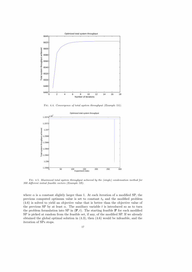
and input as network parameters into (4.5). Figures 4.3 and 4.4 show the convergencetowards satisfying all the QoS constraints including the DiffServ constraint. As shownon the figures, the convergence is extremely fast with the power allocations very closeto the optimal power allocation by the 8th GP iteration.

Example 5B. A slightly larger cellular system with 6 users is then studied.The number of users is still small enough for exhaustive search to be conducted and

15

Method System throughput P ∗1 P ∗

2 P ∗3

Exhaustive 6626 kbps 0.65 0.77 0.79searchSingle 6626 kbps by 0.65 0.77 0.78

condensation solving 17 GPsAdded DiffServ 6624 kbps by 0.68 0.75 0.68

constraint solving 17 GPs

Table 4.1

Examples 4 and 5A. Row 2 shows Example 4 using the single condensation on system throughputmaximization, and Row 1 shows the optimal solutions found by exhaustive search. Row 3 showsExample 5A with an additional DiffServ constraint D1/D3 = 1, which also recovers the new optimalsolution of 6624 kbps as verified by exhaustive search.

0 2 4 6 8 10 12 14 16 180.2

0.4

0.6

0.8

1

1.2

1.4

1.6

1.8

Number of iterations

Pow

er (

mW

)

Transmit power for each user

User 1User 2User 3

Fig. 4.3. Convergence of power variables (Example 5A).

to establish the benchmark of globally optimal power control. Performance of SPcondensation method for 300 different initial feasible power allocations is shown inFigure 4.5. With an extremely few number of exceptions, SP condensation returns theglobally optimal power allocation. By using a more relaxed but sufficiently accurateexit condition ε = 10−3, the average number of GP iterations needed is reduced to 11even though the problem size doubles compared to Example 5A.

The optimum of power control produced by the condensation method may be alocal one. The following new heuristic of solving a series of SPs (each solved througha series of GPs) can be further applied to help find the global optimum. After theoriginal SP (4.3) is solved, a slightly modified SP is formulated and solved:

minimize t

subject to∏N

i=11

1+SIRi

≤ t,

t ≤ t0α ,

Same set of constraints as problem (4.3),

(4.6)

16

0 2 4 6 8 10 12 14 16 186460

6480

6500

6520

6540

6560

6580

6600

6620

6640

Tot

al s

yste

m th

roug

hput

ach

ieve

d

Number of iterations

Optimized total system throughput

Fig. 4.4. Convergence of total system throughput (Example 5A).

0 50 100 150 200 250 3001.2358

1.236

1.2362

1.2364

1.2366

1.2368

1.237

1.2372

1.2374x 104

Experiment index

Tot

al s

yste

m th

roug

hput

ach

ieve

d

Optimized total system throughput

Fig. 4.5. Maximized total system throughput achieved by the (single) condensation method for300 different initial feasible vectors (Example 5B).

where α is a constant slightly larger than 1. At each iteration of a modified SP, theprevious computed optimum value is set to constant t0 and the modified problem(4.6) is solved to yield an objective value that is better than the objective value ofthe previous SP by at least α. The auxiliary variable t is introduced so as to turnthe problem formulation into SP in (P, t). The starting feasible P for each modifiedSP is picked at random from the feasible set, if any, of the modified SP. If we alreadyobtained the global optimal solution in (4.3), then (4.6) would be infeasible, and theiteration of SPs stops.

17

Example 4 Continued. The above heuristic is applied to the rare instances ofExample 4 where solving SP returns a locally optimal power allocation, and is foundto obtain the globally optimal solution within 1 or 2 rounds of solving additional SPs(4.6).

5. Distributed Implementation. Another limitation for GP based power con-trol is the need for centralized computation if a GP is solved by interior point methods.The GP formulations of power control problems can also be solved by a new methodof distributed algorithm for GP that is first presented in this chapter (see also [19, 7]).The basic idea is that each user solves its own local optimization problem and the cou-pling among users is taken care of by message passing among the users. Interestingly,the special structure of coupling for the problem at hand (essentially, all couplingamong the logical links can be lumped together using interference terms) allows oneto further reduce the amount of message passing among the users [19]. Specifically,we use a dual decomposition method to decompose a GP into smaller subproblemswhose solutions are jointly and iteratively coordinated by the use of dual variables.The key step is to introduce auxiliary variables and to add extra equality constraints,thus transferring the coupling in the objective to coupling in the constraints, whichcan be solved by introducing ‘consistency pricing’. We illustrate this idea through anunconstrained minimization problem followed by an application of the technique towireless network power control.

5.1. Distributed algorithm for GP. Suppose we have the following uncon-strained standard form GP in x � 0:

minimize∑

i fi(xi, {xj}j∈I(i))(5.1)

where xi denotes the local variable of the ith user, {xj}j∈I(i) denote the coupledvariables from other users, and fi is either a monomial or posynomial. Making achange of variable yi = log xi, ∀i in the original problem, we obtain

minimize∑

i fi(eyi , {eyj}j∈I(i)).

We now rewrite the problem by introducing auxiliary variables yij for the coupledarguments and additional equality constraints to enforce consistency:

minimize∑

i fi(eyi , {eyij}j∈I(i))

subject to yij = yj , ∀j ∈ I(i), ∀i.(5.2)

Each ith user controls the local variables (yi, {yij}j∈I(i)). Next, the Lagrangian of(5.2) is formed as

L({yi}, {yij}; {γij}) =∑

i

fi(eyi , {eyij}j∈I(i)) +

∑

i

∑

j∈I(i)

γij(yj − yij)

=∑

i

Li(yi, {yij}; {γij})

where

Li(yi, {yij}; {γij}) = fi(eyi , {eyij}j∈I(i)) +

(

∑

j:i∈I(j)

γji

)

yi −∑

j∈I(i)

γijyij .(5.3)

18

The minimization of the Lagrangian with respect to the primal variables ({yi}, {yij})can be done simultaneously (in a parallel fashion) by each user. In the more generalcase where the original problem (5.1) is constrained, the additional constraints canbe included in the minimization at each Li.

In addition, the following master dual problem has to be solved to obtain theoptimal dual variables or consistency prices {γij}:

max{γij}

g({γij})(5.4)

where

g({γij}) =∑

i

minyi,{yij}

Li(yi, {yij}; {γij}).

Note that the transformed primal problem (5.2) is convex, and the duality gap is zerounder mild conditions; hence the Lagrange dual problem indeed solves the originalstandard GP problem. A simple way to solve the maximization in (5.4) is with thefollowing update for the consistency prices:

γij(t + 1) = γij(t) + δ(t)(yj(t) − yij(t)).(5.5)

Appropriate choice of the stepsize δ(t) > 0 leads to stability and convergence of thedual algorithm [7].

Summarizing, the ith user has to: i) minimize the function Li in (5.3) involvingonly local variables upon receiving the updated dual variables {γji, j : i ∈ I(j)} (notethat {γij , j ∈ I(i)} are local dual variables), and ii) update the local consistency prices{γij , j ∈ I(i)} with (5.5).

5.2. Applications to power control. As an illustrative example, we maximizethe total system throughput in the high SIR regime with constraints local to each user.If we directly applied the distributed approach described in the last subsection, theresulting algorithm would not be very practical since it would require knowledge byeach user of the interfering channels and interfering transmit powers, which wouldtranslate into a large amount of message passing. To obtain a practical distributedsolution, we can leverage the structures of power control problems at hand, and insteadkeep a local copy of each of the effective received powers P R

ij = GijPj and write theproblem as follows (using the log change of variable x̃ = log x):

minimize∑

i log(

G−1ii exp(−P̃i)

(

∑

j 6=i exp(P̃ Rij ) + σ2

))

subject to P̃ Rij = G̃ij + P̃j ,

Constraints local to each user.

(5.6)

The partial Lagrangian is

L =∑

i

log

G−1ii exp(−P̃i)

∑

j 6=i

exp(P̃ Rij ) + σ2

+∑

i

∑

j 6=i

γij

(

P̃ Rij −

(

G̃ij + P̃j

))

,

from which the dual variable update is found as

γij (t + 1) = γij (t) + δ(t)(

P̃ Rij −

(

G̃ij + P̃j

))

= γij (t) + δ(t)(

P̃ Rij − log GijPj

)

.(5.7)

19

Each user has to minimize the following Lagrangian (with respect to the primal vari-ables) subject to the local constraints:

Li

(

P̃i,{

P̃ Rij

}

j; {γij}j

)

= log

G−1ii exp(−P̃i)

∑

j 6=i

exp(P̃ Rij ) + σ2

+∑

j 6=i

γij P̃Rij −

∑

j 6=i

γji

P̃i.

(5.8)Some practical observations are in order:• For the minimization of the local Lagrangian, each user only needs to know

the term(

∑

j 6=i γji

)

involving the dual variables from the interfering users,

which requires some message passing.• For the dual variable update, each user needs to know the effective received

power from each of the interfering users P Rij = GijPj for j 6= i, which in prac-

tice may be estimated from the received messages, hence no explicit messagepassing is required for this.

With this approach we have avoided the need to know all the interfering channelsGij and the powers used by the interfering users Pj . However, each user still needsto know the consistency prices from the interfering users via some message passing.This message passing can be reduced in practice by ignoring the messages from linksthat are physically far apart, leading to suboptimal distributed heuristics.

Example 6. We apply the distributed algorithm to solve the above power controlproblem for three logical links with Gij = 0.2, i 6= j, Gii = 1, ∀i, maximal transmitpowers of 6mW, 7mW and 7mW for link 1, 2 and 3 respectively. Figure 5.1 showsthe convergence of the dual objective function which is also the global optimal to-tal throughput of the links. Figure 5.2 shows the convergence of the two auxiliaryvariables in link 1 and 3 towards the optimal solutions.

0 50 100 150 2000.4

0.6

0.8

1

1.2

1.4

1.6

1.8

2

2.2x 10

4

Iteration

Dual objective function

Fig. 5.1. Convergence of the dual objective function through distributed algorithm (Example 6).

6. Conclusions. Power control problems with nonlinear objective and constraintsmay seem to be difficult to solve for global optimality. However, when SIR is much

20

0 50 100 150 200−10

−8

−6

−4

−2

0

2

Iteration

Consistency of the auxiliary variables

log(P2)

log(PR12

/G12

)

log(PR32

/G32

)

Fig. 5.2. Convergence of the consistency constraints through distributed algorithm (Example 6).

larger than 0dB, GP can be used to turn these problems, with a variety of possiblecombinations of objective and constraint functions involving data rate, delay, and out-age probability, into intrinsically tractable convex formulations. Then interior pointalgorithms can efficiently compute the globally optimal power allocation even for alarge network. Feasibility and sensitivity analysis of GP naturally lead to admissioncontrol and pricing schemes. When the high SIR approximation cannot be made, thesepower control problems become SP and may be solved by the heuristic of condensa-tion method through a series of GPs. Distributed optimal algorithms for GP-basedpower control in multihop networks can also be carried out through message passing.

Sections 4 and 5 present very recent advances overcoming the major limitationsof the original GP-based power control methods in [14]. Several interesting researchissues remain to be further explored: reduction of SP solution complexity by usinghigh-SIR approximation to obtain the initial power vector and by solving the seriesof GPs only approximately (except the last GP), combination of SP solution anddistributed algorithm for distributed power control in low SIR regime, and applicationto optimal spectrum management in DSL broadband access systems with interference-limited performance across the tones and among competing users sharing a cablebinder.

Acknowledgement. We would like to acknowledge collaborations on GP-basedresource allocation with Stephen Boyd at Stanford University and Arak Sutivong atQualcomm, and discussions with Wei Yu at the University of Toronto.

This work has been supported by Hertz Foundation Fellowship, Stanford Grad-uate Fellowship, NSF Grants CNS-0417607, CNS-0427677, CCF-0440443, and NSFCAREER Award CCF-0448012.

REFERENCES

[1] M. Avriel, Ed. Advances in Geometric Programming, Plenum Press, New York, 1980.

21

[2] N. Bambos, “Toward power-sensitive network architectures in wireless communications: Con-cepts, issues, and design aspects.” IEEE Pers. Comm. Mag., vol. 5, no. 3, pp. 50-59, 1998.

[3] C. S. Beightler and D. T. Philips, Applied Geometric Programming, Wiley 1976.[4] S. Boyd, S. J. Kim, L. Vandenberghe, and A. Hassibi, “A tutorial on geometric programming”,

Stanford University EE Technical Report, 2005.[5] S. Boyd and L. Vandenberghe, Convex Optimization, Cambridge University Press, 2004.[6] M. Chiang, “Balancing transport and physical layers in wireless multihop networks: Jointly

optimal congestion control and power control,” IEEE J. Sel. Area Comm., vol. 23, no. 1,pp. 104-116, Jan. 2005.

[7] M. Chiang, “Geometric programming for communication systems”, To appear in Foundationsand Trends of Communications and Information Theory, 2005.

[8] M. Chiang and S. Boyd, “Geometric programming duals of channel capacity and rate distortion,”IEEE Trans. Inform. Theory, vol. 50, no. 2, pp. 245-258, Feb. 2004.

[9] M. Chiang and A. Sutivong, “Efficient nonlinear optimization of resource allocation”, Proc.IEEE Globecom, San Francisco, CA, Dec. 2003.

[10] M. Chiang, A. Sutivong, and S. Boyd, “Efficient nonlinear optimizations of queuing systems,”Proc. IEEE Globecom, Taipei, ROC, Nov. 2002.

[11] R. J. Duffin, “Linearized geometric programs,” SIAM Review, vol. 12, pp. 211-227, 1970.[12] R. J. Duffin, E. L. Peterson, and C. Zener, Geometric Programming: Theory and Applications,

Wiley, 1967.[13] G. Foschini and Z. Miljanic, “A simple distributed autonomous power control algorithm and its

convergence”, IEEE Trans. Veh. Tech., vol. 42, no. 4, 1993.[14] D. Julian, M. Chiang, D. ONeill, and S. Boyd, “QoS and fairness constrained convex optimiza-

tion of resource allocation for wireless cellular and ad hoc networks.” Proc. IEEE Infocom,New York, NY, June 2002.

[15] S. Kandukuri and S. Boyd, “Optimal power control in interference limited fading wireless chan-nels with outage probability specifications”, IEEE Trans. Wireless Comm., vol. 1, no. 1, pp.46-55, Jan. 2002.

[16] K. O. Kortanek, X. Xu, and Y. Ye, “An infeasible interior-point algorithm for solving primaland dual geometric programs,” Math. Programming, vol. 76, pp. 155-181, 1996.

[17] D. Mitra, “An asynchronous distributed algorithm for power control in cellular radio systems”,Proceedings of 4th WINLAB Workshop Rutgers University, NJ, 1993.

[18] Yu. Nesterov and A. Nemirovsky, Interior Point Polynomial Methods in Convex Programming,SIAM Press, 1994.

[19] D. Palomar and M. Chiang, “Distributed algorithms for coupled utility maximization,” Workingdraft, Princeton University, 2005.

[20] C. Saraydar, N. Mandayam, and D. Goodman, “Pricing and power control in a multicell wirelessdata network”, IEEE J. Sel. Areas Comm., vol. 19, no. 10, pp. 1883-1892, 2001.

[21] C. Sung and W. Wong, “Power control and rate management for wireless multimedia CDMAsystems”, IEEE Trans. Comm. vol. 49, no. 7, pp. 1215-1226, 2001.

[22] R. Yates, “A framework for uplink power control in cellular radio systems”, IEEE J. Sel. AreasComm., vol. 13, no. 7, pp. 1341-1347, 1995.

22