POVERTYIN TIMOR-LESTE

2014

CONTENT

PREFACE 01

EXECUTIVE SUMMARY 03

INTRODUCTION 09

POVERTY MEASUREMENT METHODOLOGY I: 11CONSUMPTION-BASED WELFARE INDICATOR

Consumption as the welfare indicator 11

Constructing comparable nominal consumption 11

Changes in nominal consumption 12expenditure 2007-2014

POVERTY MEASUREMENT METHODOLOGY II: 13POVERTY LINES

District-level poverty lines 13

Food poverty line 14

Rent poverty line 15

Non-food (excluding rent) poverty line 15

Overall poverty line 15

The estimated poverty lines 17

POVERTY ESTIMATES 19

Poverty indices 19

Headcount index 15

Poverty gap index 19

Squared poverty gap index 19

Results 20

Average consumption and inequality 20

Poverty estimates: national, sectoral 20

and regional

District-level poverty estimates 21

POVERTY REDUCTION: TIMOR-LESTE IN THE 23INTERNATIONAL CONTEXT

SENSITIVITY OF POVERTY INCIDENCE 27

Calorie requirements 27

Festivities and ceremonies 29

Fieldwork team effects 30

HOUSEHOLD CHARACTERISTICS AND POVERTY 32

Demography and poverty 32

Consumption pattern and poverty 35

Nutritional status of children 35

Ownership of livestock and other durable goods 35

MULTIDIMENSIONAL DEPRIVATION AND POVERTY 39

Annex A: Timor-Leste Survey of Living 42Standards-3

Annex B: Consumption-based welfare indicator 45

Annex C: Rental model 49

Annex D: Standard errors and 50confidence intervals

Annex E: Sensitivity analysis: fieldwork teams 52

Annex F: Issue in developing a multidimensional 57poverty index for Timor-Leste

REFERENCES 63

P O V

T I M O RL E S T E

E R T Y

01

Pov

erty

in T

imor

-Les

te 2

014

PREFACE

This report provides a detailed assessment of the

methodological approaches and headline poverty

results from the Timor-Leste Survey of Living

Standards 3. The survey is the third in a series of

mutually comparable, detailed surveys to assess a

wide range of aspects of living standards in Timor-

Leste. Over time, the Timor-Leste Surveys of Living

Standards (TLSLS) have become larger to allow for

greater precision and depth of analysis. TLSLS-1 was

conducted in 2001 soon after Timor-Leste became

an independent nation. TLSLS-1 surveyed 1,800

households over a period of three months. Six years

later, TLSLS-2 began, in 2007, and included 4,477

households surveyed over 12 months.

This survey, TLSLS-3, is the latest in the series. It

was conducted over a 12 month period from April

2014 to April 2015 and involved surveys of 5,916

households, 30 percent more than the previous

survey. A focus of the series has been to conduct

high-quality surveys that provide a sound basis for

the monitoring of household living standards, and

the critical task of designing public policy to help

improve living standards for all. TLSLS-3 marks the

highest level of survey design and implementation by

the General Directorate of Statistics, with technical

support from the World Bank. The result is a very

comprehensive, high-quality survey.

As opposed to the first two TLSLS which both followed

periods of instability and upheaval, the intervening

period between TLSLS-2 and TLSLS-3 has been one

of peace, development and stability in Timor-Leste.

It is therefore important to reflect upon the impact

that a stable country with an ambitious development

agenda can have on improving living standard when

not set back by periods of conflict or disasters.

This report focuses on providing key results from

the TLSLS-3 and a detailed account of the survey

methods. These is not the end but marks the

beginning of an exercise to exploit the rich detail of

the data-source, and the Government of Timor-Leste

in coordination with its development partners and

research community will be conducting further work

to assess the drivers of poverty, and help to design

policy and interventions that have the biggest positive

impact for the most people.

Dili, September 2016

Helder Lopes

Vice-Minister of Finance

T I M O RL E S T E

E R T Y

0302

Pov

erty

in T

imor

-Les

te 2

014

Pov

erty

in T

imor

-Les

te 2

014

EXECUTIVESUMMARY

INTRODUCTION

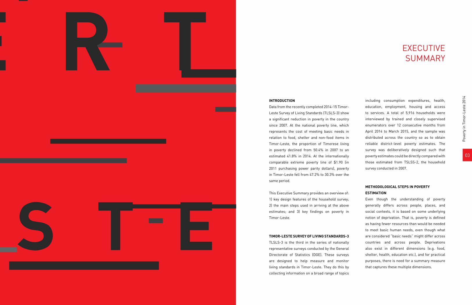
Data from the recently completed 2014-15 Timor-

Leste Survey of Living Standards (TLSLS-3) show

a significant reduction in poverty in the country

since 2007. At the national poverty line, which

represents the cost of meeting basic needs in

relation to food, shelter and non-food items in

Timor-Leste, the proportion of Timorese living

in poverty declined from 50.4% in 2007 to an

estimated 41.8% in 2014. At the internationally

comparable extreme poverty line of $1.90 (in

2011 purchasing power parity dollars), poverty

in Timor-Leste fell from 47.2% to 30.3% over the

same period.

This Executive Summary provides an overview of:

1) key design features of the household survey;

2) the main steps used in arriving at the above

estimates; and 3) key findings on poverty in

Timor-Leste.

TIMOR-LESTE SURVEY OF LIVING STANDARDS-3

TLSLS-3 is the third in the series of nationally

representative surveys conducted by the General

Directorate of Statistics (DGE). These surveys

are designed to help measure and monitor

living standards in Timor-Leste. They do this by

collecting information on a broad range of topics

including consumption expenditures, health,

education, employment, housing and access

to services. A total of 5,916 households were

interviewed by trained and closely supervised

enumerators over 12 consecutive months from

April 2014 to March 2015, and the sample was

distributed across the country so as to obtain

reliable district-level poverty estimates. The

survey was deliberatively designed such that

poverty estimates could be directly compared with

those estimated from TSLSS-2, the household

survey conducted in 2007.

METHODOLOGICAL STEPS IN POVERTY

ESTIMATION

Even though the understanding of poverty

generally differs across people, places, and

social contexts, it is based on some underlying

notion of deprivation. That is, poverty is defined

as having fewer resources than would be needed

to meet basic human needs, even though what

are considered “basic needs” might differ across

countries and across people. Deprivations

also exist in different dimensions (e.g. food,

shelter, health, education etc.), and for practical

purposes, there is need for a summary measure

that captures these multiple dimensions.

P O V

T I M O RL E S T E

E R T Y

0504

Pov

erty

in T

imor

-Les

te 2

014

Pov

erty

in T

imor

-Les

te 2

014

This report provides key results using (i) a

consumption-based indicator that aggregates

deprivations in multiple dimensions in monetary

terms and (ii) a set of non-monetary indicators

that directly capture specific deprivations in

key dimensions. A consumption-based rather

than income-based measure is used because

information on consumption is more easily and

accurately collected than information on income

given the large subsistence and informal sectors in

the economy. In addition, non-monetary indicators

are used to assess deprivations in specific

dimensions that are not completely captured by

monetary measures, such as health, education,

and ownership of essential assets.

Consumption-based poverty measures. The

consumption-based indicator is per capita total

household expenditure which consists of three

key components: 1) the value food expenditures

(purchased as well as own-produced); 2) the rental

value of dwellings (actual or imputed); and 3) the

value of all other non-food, non-rent expenditures.

The values of food and non-food consumption

were directly computed from TLSLS-3 responses.

For rent, as most dwellings are owner-occupied

and few people actually pay rent, the value of

rent is imputed with the commonly-used hedonic

regression approach. The hedonic model uses the

relationship between respondents’ estimates of

actual rent paid (when available) or how much their

dwelling could be rented for and the characteristics

of the dwelling to estimate market values of

dwellings with specific characteristics.

The consumption-based poverty line is the sum of

three components: 1) the food poverty line; 2) the

rental poverty line; and 3) the non-food non-rent

poverty line. The food poverty line is derived as

the cost of the typical local food basket that yields

a nutrient value of 2,100 calories per person. The

rental poverty line is the average estimated rental

cost of a reference dwelling that has 2 rooms,

good external walls, proper sanitation and access

to electricity. Finally, the non-food poverty line is

specified as the average non-food expenditure of

those households whose food expenditures are

close to the food poverty line.

KEY STEPS IN MEASURING POVERTY

1. Per capita total consumption expenditure is used to measure welfare.

2. A poverty line, also expressed in per capita consumption expenditure, is specified as the

monetary value of a 2,100 calorie per day diet, living in a 2 room home with proper

sanitation and access to electricity, and a corresponding consumption level of non-food

goods and services.

3. The following poverty indices are used to summarize the level of poverty:

Poverty headcount index: The proportion of the total population below the poverty line.

Poverty gap Index: A measure of the average amount by which a family’s consumption

falls short of the poverty line expressed as a proportion of the poverty line, while the

consumption shortfall of those above the poverty line is taken to be zero.

Given the objective of generating district-level

poverty estimates, poverty lines were estimated

separately for each district, accounting for

differences in consumption patterns as well as

commodity prices. Given the smaller sample sizes

at district level, the margins of error are higher

for district-level estimates. The key steps used in

estimating poverty prevalence are summarized in

the Box 1. Details on these steps are discussed in

Sections 2 and 3.

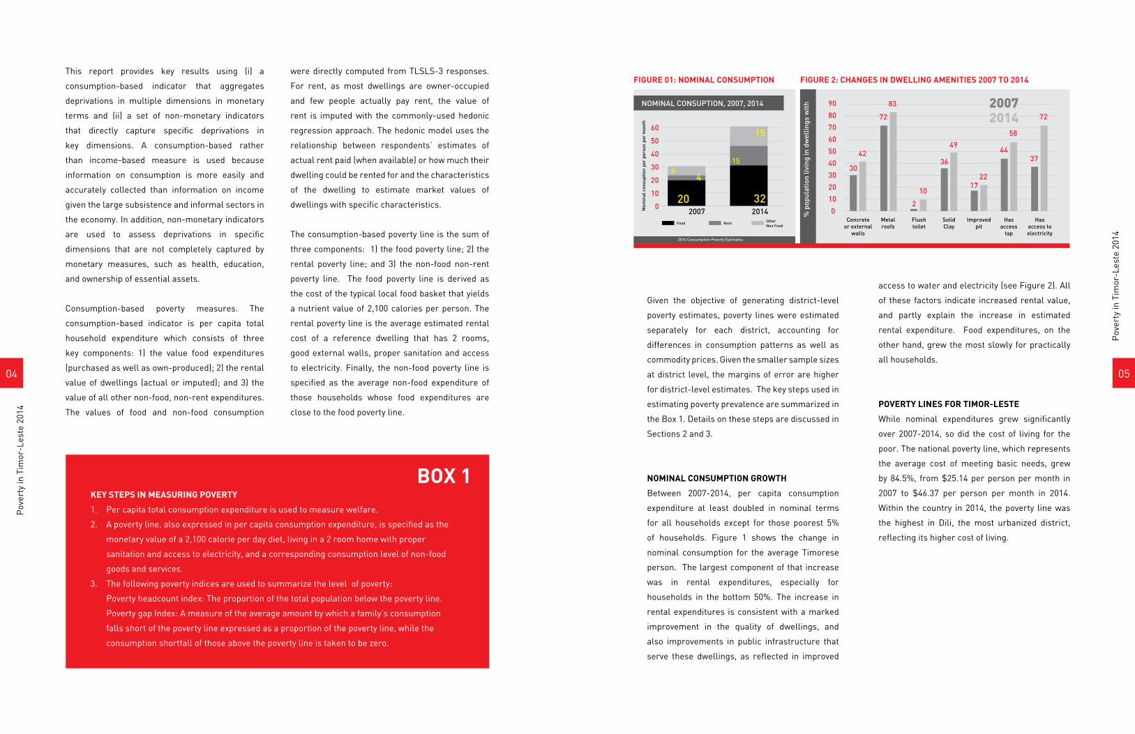
NOMINAL CONSUMPTION GROWTH

Between 2007-2014, per capita consumption

expenditure at least doubled in nominal terms

for all households except for those poorest 5%

of households. Figure 1 shows the change in

nominal consumption for the average Timorese

person. The largest component of that increase

was in rental expenditures, especially for

households in the bottom 50%. The increase in

rental expenditures is consistent with a marked

improvement in the quality of dwellings, and

also improvements in public infrastructure that

serve these dwellings, as reflected in improved

access to water and electricity (see Figure 2). All

of these factors indicate increased rental value,

and partly explain the increase in estimated

rental expenditure. Food expenditures, on the

other hand, grew the most slowly for practically

all households.

POVERTY LINES FOR TIMOR-LESTE

While nominal expenditures grew significantly

over 2007-2014, so did the cost of living for the

poor. The national poverty line, which represents

the average cost of meeting basic needs, grew

by 84.5%, from $25.14 per person per month in

2007 to $46.37 per person per month in 2014.

Within the country in 2014, the poverty line was

the highest in Dili, the most urbanized district,

reflecting its higher cost of living.

FIGURE 01: NOMINAL CONSUMPTION FIGURE 2: CHANGES IN DWELLING AMENITIES 2007 TO 2014

% p

opul

atio

n liv

ing

in d

wel

lings

wit

h

60

70

80

90

50

40

30

20

10

30

42

72

83 20072014

2

10

36

49

1722

44

58

0Concrete

or externalwalls

Metalroofs

Flushtoilet

SolidClay

Improvedpit

Hasaccess

tap

Hasaccess toelectricity

37

72

6

60

50

40

30

20

10

0

15

15

32

4

20

NOMINAL CONSUPTION, 2007, 2014

Nom

inal

con

supt

ion

per

pers

on p

er m

onth

Food

2007 2014Rent Other

Non Food

2014 Consumption Poverty Estimates

BOX 1

0706

Pov

erty

in T

imor

-Les

te 2

014

Pov

erty

in T

imor

-Les

te 2

014

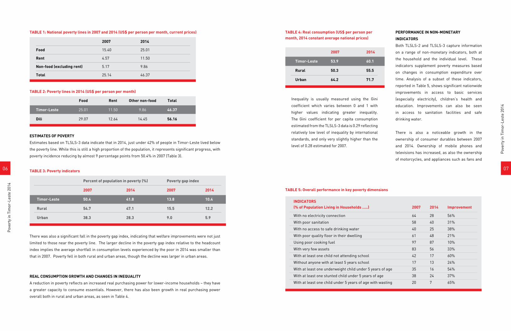
ESTIMATES OF POVERTY

Estimates based on TLSLS-3 data indicate that in 2014, just under 42% of people in Timor-Leste lived below

the poverty line. While this is still a high proportion of the population, it represents significant progress, with

poverty incidence reducing by almost 9 percentage points from 50.4% in 2007 (Table 3).

There was also a significant fall in the poverty gap index, indicating that welfare improvements were not just

limited to those near the poverty line. The larger decline in the poverty gap index relative to the headcount

index implies the average shortfall in consumption levels experienced by the poor in 2014 was smaller than

that in 2007. Poverty fell in both rural and urban areas, though the decline was larger in urban areas.

REAL CONSUMPTION GROWTH AND CHANGES IN INEQUALITY

A reduction in poverty reflects an increased real purchasing power for lower-income households – they have

a greater capacity to consume essentials. However, there has also been growth in real purchasing power

overall both in rural and urban areas, as seen in Table 4.

TABLE 3: Poverty indicators

TABLE 2: Poverty lines in 2014 (US$ per person per month)

TABLE 1: National poverty lines in 2007 and 2014 (US$ per person per month, current prices)

TABLE 5: Overall performance in key poverty dimensions

2007 2014

Food 15.40 25.01

Rent 4.57 11.50

Non-food (excluding rent) 5.17 9.86

Total 25.14 46.37

Inequality is usually measured using the Gini

coefficient which varies between 0 and 1 with

higher values indicating greater inequality.

The Gini coefficient for per capita consumption

estimated from the TLSLS-3 data is 0.29 reflecting

relatively low level of inequality by international

standards, and only very slightly higher than the

level of 0.28 estimated for 2007.

PERFORMANCE IN NON-MONETARY

INDICATORS

Both TLSLS-2 and TLSLS-3 capture information

on a range of non-monetary indicators, both at

the household and the individual level. These

indicators supplement poverty measures based

on changes in consumption expenditure over

time. Analysis of a subset of these indicators,

reported in Table 5, shows significant nationwide

improvements in access to basic services

(especially electricity), children’s health and

education. Improvements can also be seen

in access to sanitation facilities and safe

drinking water.

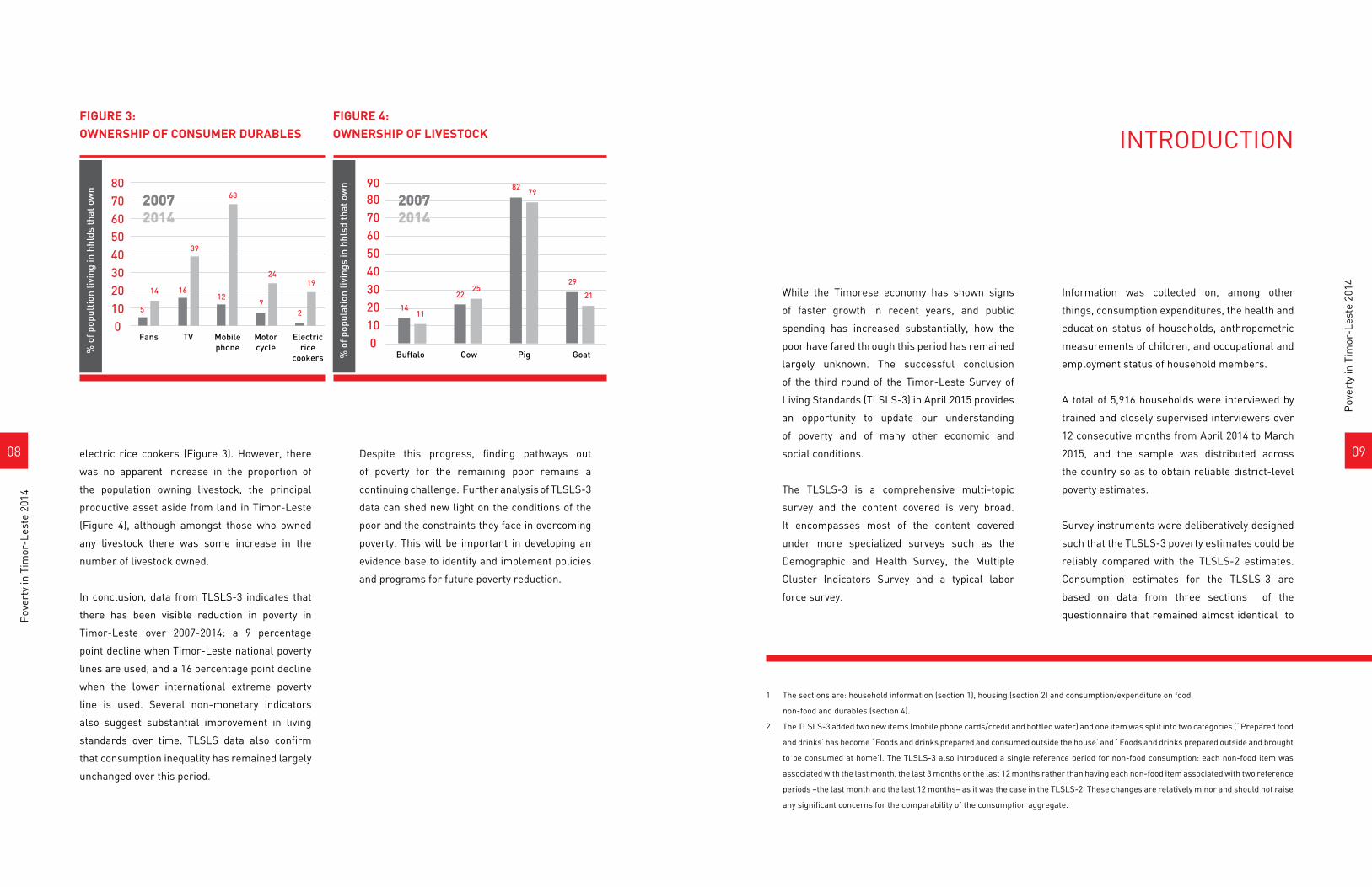
There is also a noticeable growth in the

ownership of consumer durables between 2007

and 2014. Ownership of mobile phones and

televisions has increased, as also the ownership

of motorcycles, and appliances such as fans and

TABLE 4: Real consumption (US$ per person per month, 2014 constant average national prices)

2007 2014

Timor-Leste 53.9 60.1

Rural 50.3 55.5

Urban 64.2 71.7

Food Rent Other non-food Total

Timor-Leste 25.01 11.50 9.86 46.37

Dili 29.07 12.64 14.45 56.16

Percent of population in poverty (%) Poverty gap index

2007 2014 2007 2014

Timor-Leste 50.4 41.8 13.8 10.4

Rural 54.7 47.1 15.5 12.2

Urban 38.3 28.3 9.0 5.9

INDICATORS (% of Population Living in Households …..) 2007 2014 Improvement

With no electricity connection 64 28 56%

With poor sanitation 58 40 31%

With no access to safe drinking water 40 25 38%

With poor quality floor in their dwelling 61 48 21%

Using poor cooking fuel 97 87 10%

With very few assets 83 56 33%

With at least one child not attending school 42 17 60%

Without anyone with at least 5 years school 17 13 24%

With at least one underweight child under 5 years of age 35 16 54%

With at least one stunted child under 5 years of age 38 24 37%

With at least one child under 5 years of age with wasting 20 7 65%

0908

Pov

erty

in T

imor

-Les

te 2

014

Pov

erty

in T

imor

-Les

te 2

014

While the Timorese economy has shown signs

of faster growth in recent years, and public

spending has increased substantially, how the

poor have fared through this period has remained

largely unknown. The successful conclusion

of the third round of the Timor-Leste Survey of

Living Standards (TLSLS-3) in April 2015 provides

an opportunity to update our understanding

of poverty and of many other economic and

social conditions.

The TLSLS-3 is a comprehensive multi-topic

survey and the content covered is very broad.

It encompasses most of the content covered

under more specialized surveys such as the

Demographic and Health Survey, the Multiple

Cluster Indicators Survey and a typical labor

force survey.

Information was collected on, among other

things, consumption expenditures, the health and

education status of households, anthropometric

measurements of children, and occupational and

employment status of household members.

A total of 5,916 households were interviewed by

trained and closely supervised interviewers over

12 consecutive months from April 2014 to March

2015, and the sample was distributed across

the country so as to obtain reliable district-level

poverty estimates.

Survey instruments were deliberatively designed

such that the TLSLS-3 poverty estimates could be

reliably compared with the TLSLS-2 estimates.

Consumption estimates for the TLSLS-3 are

based on data from three sections of the

questionnaire that remained almost identical to

electric rice cookers (Figure 3). However, there

was no apparent increase in the proportion of

the population owning livestock, the principal

productive asset aside from land in Timor-Leste

(Figure 4), although amongst those who owned

any livestock there was some increase in the

number of livestock owned.

In conclusion, data from TLSLS-3 indicates that

there has been visible reduction in poverty in

Timor-Leste over 2007-2014: a 9 percentage

point decline when Timor-Leste national poverty

lines are used, and a 16 percentage point decline

when the lower international extreme poverty

line is used. Several non-monetary indicators

also suggest substantial improvement in living

standards over time. TLSLS data also confirm

that consumption inequality has remained largely

unchanged over this period.

Despite this progress, finding pathways out

of poverty for the remaining poor remains a

continuing challenge. Further analysis of TLSLS-3

data can shed new light on the conditions of the

poor and the constraints they face in overcoming

poverty. This will be important in developing an

evidence base to identify and implement policies

and programs for future poverty reduction.

1 The sections are: household information (section 1), housing (section 2) and consumption/expenditure on food,

non-food and durables (section 4).

2 The TLSLS-3 added two new items (mobile phone cards/credit and bottled water) and one item was split into two categories (`Prepared food

and drinks’ has become ̀ Foods and drinks prepared and consumed outside the house’ and ̀ Foods and drinks prepared outside and brought

to be consumed at home’). The TLSLS-3 also introduced a single reference period for non-food consumption: each non-food item was

associated with the last month, the last 3 months or the last 12 months rather than having each non-food item associated with two reference

periods –the last month and the last 12 months– as it was the case in the TLSLS-2. These changes are relatively minor and should not raise

any significant concerns for the comparability of the consumption aggregate.

INTRODUCTION

5

14

20072014

Fans TV Mobilephone

Motorcycle

Electricrice

cookers

1612

39

72

2419

68

% o

f pop

ulti

on li

ving

in h

hlds

that

ow

n

607080

50403020100

20072014

Buffalo Cow Pig Goat

1411

2225

8279

29

21

% o

f pop

ulat

ion

livin

gs in

hhl

sd th

at o

wn

60708090

50403020100

FIGURE 3:OWNERSHIP OF CONSUMER DURABLES

FIGURE 4:OWNERSHIP OF LIVESTOCK

1110

Pov

erty

in T

imor

-Les

te 2

014

Pov

erty

in T

imor

-Les

te 2

014

The main methodological consideration in

constructing new estimates of poverty with the

TLSLS-3 data is to construct estimates that

are comparable with the 2007 TLSLS-2 poverty

estimates and are consistent across space. This

in turn implies considerations relating to (a)

using consumption as the welfare indicator, (b)

constructing comparable estimates of nominal

consumption, and (c) constructing a set of poverty

lines for 2014 that reflect, as far as possible, the

same standard of living as the poverty lines for

2007. Section 2 covers the first two considerations,

and the latter will be covered in Section 3.

CONSUMPTION AS THE WELFARE INDICATOR

The decision to use total consumption expenditure

(including some imputed expenditures as

discussed below) rather than income as the

measure of individual welfare is motivated by

two main considerations. First, consumption is

arguably a more appropriate indicator if we are

concerned with realized, rather than potential

welfare, since not all income is consumed, nor all

consumption financed out of income. Individuals

use savings and credit to smooth fluctuations

in income and therefore consumption provides

a more accurate measure of an individual’s

welfare over time. Second, similar to many

other developing countries with large informal

sectors, in Timor Leste, consumption tends to

be measured more accurately than income in

household surveys. This is largely due to the

difficulties in defining and measuring income for

the self-employed who account for a relatively

large proportion of the work force.

As in the TLSLS-2 poverty estimates, per capita

household consumption is used as the basic

measure of individual welfare. While this measure

does not incorporate some important aspects of

individual welfare, such as consumption of public

goods (for example, schools, health services,

public sewage facilities), it is a useful aggregate

money metric of welfare that reflects individual

preferences conditional on prices and incomes,

and for that reason, is widely used in welfare

assessment and poverty monitoring.

CONSTRUCTING COMPARABLE NOMINAL

CONSUMPTION

Having selected consumption as the measure of

welfare, the first task in constructing comparable

poverty measures is to construct comparable

estimates of nominal consumption for every

household. Household nominal consumption has

three components: (i) food, (ii) rent as the value

the TLSLS 2007. The two surveys followed highly

comparable fieldwork protocols, even though

the TLSLS-3 canvassed a substantially larger

sample. Further details on TLSLS-3 are provided

in Annex A.

Using these new data, this report presents

comparable estimates of poverty. The primary

focus is on poverty measured in terms of

household consumption expenditure, an

important indicator of wellbeing. The construction

of this consumption-based poverty measures is

discussed in Sections 2 through 5.

Of course, consumption poverty provides only

a partial window on deprivation and well-

being of the population. So this assessment is

supplemented with a further look at progress in

other “non-income” dimensions of welfare. The

last section of this report presents estimates for

several such non-income indicators as building

blocks for an analysis of multidimensional poverty

in Timor-Leste. Finally, Annex F suggests options

for future work on constructing multidimensional

poverty measures for the country.

POVERTY MEASUREMENT METHODOLOGY I:

CONSUMPTION-BASEDWELFARE INDICATOR

1312

Pov

erty

in T

imor

-Les

te 2

014

Pov

erty

in T

imor

-Les

te 2

014

of housing services consumed by the household,

and (iii) other non-food goods and services.

The food and non-food components are directly

estimated from the survey data based on the

reported value of the food and non-food items

consumed. This follows the same procedures as

in the TLSLS-2 survey (see Annex B for details).

However, most houses in Timor-Leste are owner

occupied and the rental market in the country

is thin. Hence reported rent in the survey is not

actual rent, but respondents-estimated rent and

this is subject to measurement errors. For this

reason, information on estimated rents is not used

directly. Instead, when constructing the rental

component, actual rents are used whenever

available, and predicted (imputed) rents are

used otherwise. These predictions are obtained

from a hedonic rental model that estimates the

relationship between reported rental values and

a number of observable dwelling characteristics

(number of rooms, building materials used etc.).

Such a model had earlier been estimated with the

TLSLS-2 data to evaluate the rental component

of household consumption in 2007 (World Bank,

2008). A similar model is estimated now with

TLSLS-3 data to calculate the rental component

of household consumption in 2014. The estimated

rental models for 2007 and 2014 are shown in

Annex C.

CHANGES IN NOMINAL CONSUMPTION

EXPENDITURE 2007-2014

Figure 1 shows the growth in nominal

consumption per capita between 2007 (TLSLS-2)

and 2014 (TLSLS-3). It is notable that at least in

nominal terms, rent has been the fastest growing

component of consumption and food has been

the slowest component. Correspondingly, food

budget shares have declined over the two survey

periods, which in view of Engel’s law (income

elasticity of food being typically less than one)

is suggestive of improvements in the standards

of living. The substantial increase in nominal

rents and the rental share of consumption also

point to the need for more attention to the rental

component of the poverty lines.

POVERTY MEASUREMENT METHODOLOGY II: POVERTY LINES

FIGURE 1:GROWTH IN NOMINAL

CONSUMPTION BY CENTILE, 2007-2014

(PERCENT INCREASE)

Source:TLSLS 2007

and TLSLS 2014.

0

0

100

200

300

400

500

600

%

10 20 30 40 50 60 70 80 90 100

Percentile of total nominal comsuption per person

Total

Other nonfood

Food

Rent

DISTRICT-LEVEL POVERTY LINES

In the case of the TLSLS-2, poverty lines were

constructed for six domains: the rural and

urban segments of three regions (Table 1) as the

TLSLS-2 sample size permitted only this degree

of spatial disaggregation of the poverty lines.

Given the above, two main approaches can be

considered for the construction of poverty lines

for the TLSLS-3 in 2014: (i) updating the 2007

poverty lines for the six domains using estimates

of changes in the cost of living for the six domains,

or (ii) constructing a new set of poverty lines using

TLSLS-3 data and achieving comparability by

using the same methodology as in 2007.

Updating the poverty lines is restrictive in that it

limits the spatial disaggregation of the poverty

lines for 2014 to the same six domains for which

poverty lines were constructed for 2007. The

TLSLS-3, on the hand, has a 33 percent larger

sample size so that poverty statistics can be

disaggregated at the district level. Statistics at

the district level have greater policy relevance

because districts are the key administrative

units. Given that poverty statistics at the district

level are best constructed with poverty lines

determined at the district level, a continuation

of the legacy of the TLSLS-2 of six domains for

determining poverty lines appears now both

undesirable as well as unnecessary. Hence,

exploiting the larger sample size of the TLSLS-3,

which is representative at the district level,

poverty lines in 2014 are estimated separately for

the 13 districts.

The minimum sample size in the TLSLS-3

amongst the 13 districts was 254 households in

Aileu district and the median sample size was 419

households. These sample sizes are somewhat

lower than corresponding sizes for the six

domains for 2007 (Table 2), but nonetheless offer

an acceptable level of precision for the estimation

of poverty line. This new opportunity for further

spatial disaggregation is the primary motivation

for a move to district-level poverty lines with the

TLSLS-3.

TABLE 1: REGIONS, DOMAINS AND DISTRICTS

Regions Domains Districts

EAST East Urban Baucau, Lautem

and East Rural and Viqueque

CENTRE Centre Urban Aileu, Ainaro, Dili,

and Centre Rural Ermera, Liquica,

Manufahi, Manututo

WEST West Urban Bobonaro, Cova Lima

and West Rural and Oecussi

1514

Pov

erty

in T

imor

-Les

te 2

014

Pov

erty

in T

imor

-Les

te 2

014

determined as the average (per capita) quantities

of food items consumed by households belonging

to the reference group of the poor who live in that

particular domain.

The domain-specific average food bundles of

the poor are scaled up (or down) to yield the

recommended 2,100 calories per person per day.

The scaled bundles are then valued using median

prices (unit-values) of food items paid by the poor

in each domain to obtain the food poverty line for

that domain.

Rent poverty line

The rent poverty lines represent the average

imputed rental cost per person of a reference

dwelling in each domain. These lines are

constructed using a hedonic rental model

where the actual or estimated rents reported

by households are modelled as a function of

a number of the dwelling characteristics and

domain fixed effects. This is the same model as

that used for estimating the rental component of

household consumption as discussed in section

2.1 above. The model uses similar specifications

for 2007 and 2014, the only difference between

the two years is that the fixed effects refer to the

six domains for 2007, while they refer to the 13

districts for 2014.

The estimated parameters are then used to derive

the cost of a reference dwelling that is kept fixed

across domains and over the two surveys and

the rent poverty lines by domain are calculated

by dividing the predicted cost of the reference

dwelling in each domain by the corresponding

average household size of the poor in

that domain3.

As the procedure involves making predictions

over samples for two periods, a parsimonious

specification with only six dwelling characteristics

is used4. The reference dwelling for the rent

poverty lines is assumed to have 2 rooms, good

external walls, proper sanitation and access to

electricity. The estimated models are shown in

Annex C.

Non-food (excluding rent) poverty line

The non-food (excluding rent)5 poverty lines are

estimated in terms of what the poor actually

spend on non-food items. For any given domain,

the non-food poverty line corresponds to the

average per capita non-food consumption of the

population whose actual combined per capita

food and rent consumption is within plus/minus

5% of the sum of the food and rent poverty lines

for that domain.

Overall poverty line

The overall poverty line for a domain is the sum of

the food poverty line, the rent poverty line and the

non-food poverty line for that domain.

It is also worth noting that developing district-level

poverty lines is a more forward-looking approach.

It is reasonable to presume that the sample size

for future rounds of the TLSLS will grow. Thus,

it will be increasingly inappropriate and less

defensible to continue with the framework of six

spatial domains inherited from the 2007 TLSLS for

the future. Establishing a new baseline of district-

level poverty lines now will assist in monitoring

district-level trends in poverty in the future.

Before describing the new approach in detail, it is

also worth noting that in moving to the district as

the level of disaggregation for poverty lines, we,

in the process, lose the urban-rural split. The

TLSLS-3 sample size is simply not large enough

to disaggregate by both district and urban-

rural segments. However, this does not imply

that urban-rural cost of living differentials are

totally ignored under this approach. To the extent

districts differ in their degree of “urbanity”, the

district-specific poverty lines will build in cost

of living differentials due to higher or lower

representation of urban areas across districts.

For instance, a higher poverty line for Dili will

reflect, in part, the higher urban cost of living for

its largely urban population.

The comparability of district-level poverty lines in

2014 with 2007 is achieved by using exactly the

same approach to the construction of poverty

lines in 2014 as in 2007, although at a lower

level of aggregation (i.e., for 13 districts for 2014

relative to the six domains in 2007).

Poverty lines for both years are determined using

the cost of basic needs approach (Ravallion 2008).

This method effectively calculates the poverty

line as the cost of a consumption bundle that is

(i) consistent with the consumption pattern of

the poor and (ii) deemed adequate for meeting

basic needs. The poverty line has three main

components: food, rent and non-food.

Food poverty line

The food poverty line is anchored to the

recommended nutritional norm of 2,100 calories

per person. For each of the six domains in

2007 and for each of the 13 districts in 2014,

representative food bundles for the poor are

constructed to correspond to the average food

consumption pattern of the poor in that domain.

A national reference group representing the poor

is identified, and the food bundle for a particular

domain (6 in 2007 and 13 in 2014) is then

TABLE 2: COMPARING MINIMUM SAMPLE SIZES

TLSLS-3 TLSLS-2

Total sample size 5,916 households from 400 PSUs 4,477 households from 300 PSUs

Minimum sample size 254 households in Aileu district 375 households in East Urban domainin district or domain

Median sample size 419 households 695 households per district or domain

3 The average household size of the poor by domain is estimated taking into account only households that belong to the same national

reference group of poor households used for the estimation of the food poverty lines.

4 A parsimonious specification helps ward against “out-of-sample” forecasting errors that may result from the inclusion of variables that

are only marginally significant or insignificant in one of the two periods.

5 Hereafter, non-food always refers to remaining non-food excluding rent.

1716

Pov

erty

in T

imor

-Les

te 2

014

Pov

erty

in T

imor

-Les

te 2

014

than 5%. For both 2007 and 2014, it took only

two iterations for the poverty lines to converge

to the final estimates.

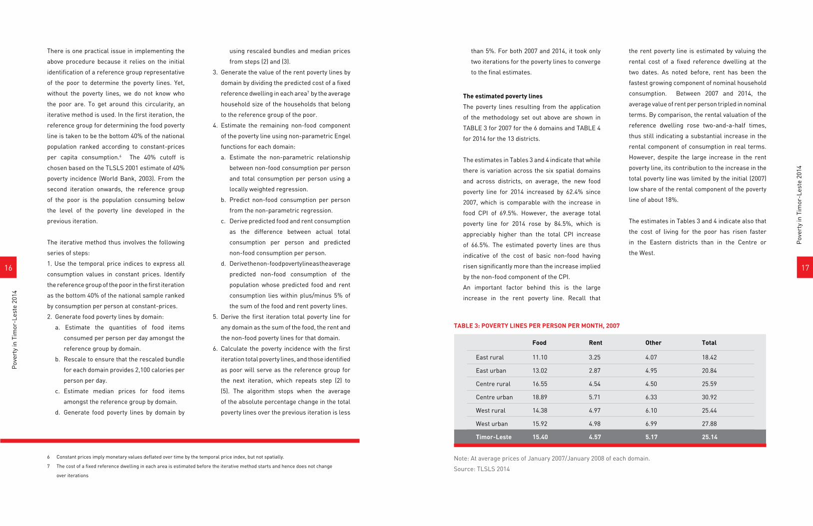
The estimated poverty lines

The poverty lines resulting from the application

of the methodology set out above are shown in

TABLE 3 for 2007 for the 6 domains and TABLE 4

for 2014 for the 13 districts.

The estimates in Tables 3 and 4 indicate that while

there is variation across the six spatial domains

and across districts, on average, the new food

poverty line for 2014 increased by 62.4% since

2007, which is comparable with the increase in

food CPI of 69.5%. However, the average total

poverty line for 2014 rose by 84.5%, which is

appreciably higher than the total CPI increase

of 66.5%. The estimated poverty lines are thus

indicative of the cost of basic non-food having

risen significantly more than the increase implied

by the non-food component of the CPI.

An important factor behind this is the large

increase in the rent poverty line. Recall that

the rent poverty line is estimated by valuing the

rental cost of a fixed reference dwelling at the

two dates. As noted before, rent has been the

fastest growing component of nominal household

consumption. Between 2007 and 2014, the

average value of rent per person tripled in nominal

terms. By comparison, the rental valuation of the

reference dwelling rose two-and-a-half times,

thus still indicating a substantial increase in the

rental component of consumption in real terms.

However, despite the large increase in the rent

poverty line, its contribution to the increase in the

total poverty line was limited by the initial (2007)

low share of the rental component of the poverty

line of about 18%.

The estimates in Tables 3 and 4 indicate also that

the cost of living for the poor has risen faster

in the Eastern districts than in the Centre or

the West.

There is one practical issue in implementing the

above procedure because it relies on the initial

identification of a reference group representative

of the poor to determine the poverty lines. Yet,

without the poverty lines, we do not know who

the poor are. To get around this circularity, an

iterative method is used. In the first iteration, the

reference group for determining the food poverty

line is taken to be the bottom 40% of the national

population ranked according to constant-prices

per capita consumption.6 The 40% cutoff is

chosen based on the TLSLS 2001 estimate of 40%

poverty incidence (World Bank, 2003). From the

second iteration onwards, the reference group

of the poor is the population consuming below

the level of the poverty line developed in the

previous iteration.

The iterative method thus involves the following

series of steps:

1. Use the temporal price indices to express all

consumption values in constant prices. Identify

the reference group of the poor in the first iteration

as the bottom 40% of the national sample ranked

by consumption per person at constant-prices.

2. Generate food poverty lines by domain:

a. Estimate the quantities of food items

consumed per person per day amongst the

reference group by domain.

b. Rescale to ensure that the rescaled bundle

for each domain provides 2,100 calories per

person per day.

c. Estimate median prices for food items

amongst the reference group by domain.

d. Generate food poverty lines by domain by

using rescaled bundles and median prices

from steps (2) and (3).

3. Generate the value of the rent poverty lines by

domain by dividing the predicted cost of a fixed

reference dwelling in each area7 by the average

household size of the households that belong

to the reference group of the poor.

4. Estimate the remaining non-food component

of the poverty line using non-parametric Engel

functions for each domain:

a. Estimate the non-parametric relationship

between non-food consumption per person

and total consumption per person using a

locally weighted regression.

b. Predict non-food consumption per person

from the non-parametric regression.

c. Derive predicted food and rent consumption

as the difference between actual total

consumption per person and predicted

non-food consumption per person.

d. Derive the non-food poverty line as the average

predicted non-food consumption of the

population whose predicted food and rent

consumption lies within plus/minus 5% of

the sum of the food and rent poverty lines.

5. Derive the first iteration total poverty line for

any domain as the sum of the food, the rent and

the non-food poverty lines for that domain.

6. Calculate the poverty incidence with the first

iteration total poverty lines, and those identified

as poor will serve as the reference group for

the next iteration, which repeats step (2) to

(5). The algorithm stops when the average

of the absolute percentage change in the total

poverty lines over the previous iteration is less

6 Constant prices imply monetary values deflated over time by the temporal price index, but not spatially.

7 The cost of a fixed reference dwelling in each area is estimated before the iterative method starts and hence does not change

over iterations

Note: At average prices of January 2007/January 2008 of each domain.

Source: TLSLS 2014

TABLE 3: POVERTY LINES PER PERSON PER MONTH, 2007

Food Rent Other Total

East rural 11.10 3.25 4.07 18.42

East urban 13.02 2.87 4.95 20.84

Centre rural 16.55 4.54 4.50 25.59

Centre urban 18.89 5.71 6.33 30.92

West rural 14.38 4.97 6.10 25.44

West urban 15.92 4.98 6.99 27.88

Timor-Leste 15.40 4.57 5.17 25.14

1918

Pov

erty

in T

imor

-Les

te 2

014

Pov

erty

in T

imor

-Les

te 2

014

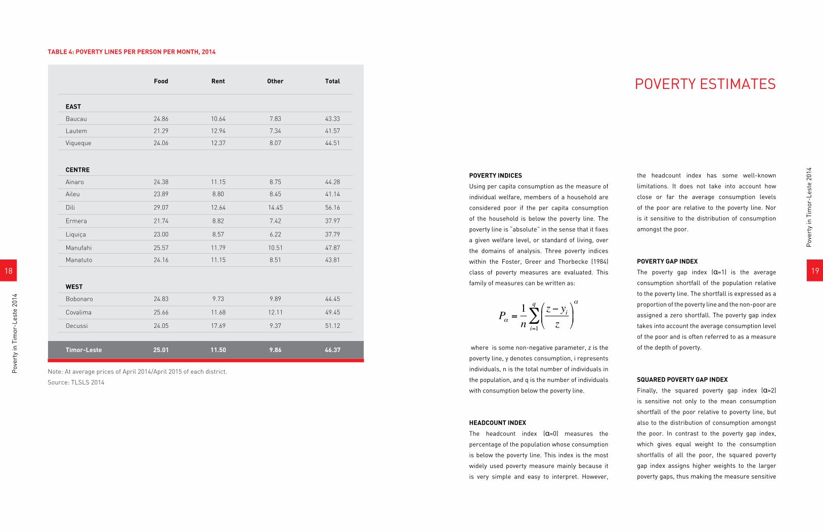
POVERTY INDICES

Using per capita consumption as the measure of

individual welfare, members of a household are

considered poor if the per capita consumption

of the household is below the poverty line. The

poverty line is “absolute” in the sense that it fixes

a given welfare level, or standard of living, over

the domains of analysis. Three poverty indices

within the Foster, Greer and Thorbecke (1984)

class of poverty measures are evaluated. This

family of measures can be written as:

where is some non-negative parameter, z is the

poverty line, y denotes consumption, i represents

individuals, n is the total number of individuals in

the population, and q is the number of individuals

with consumption below the poverty line.

HEADCOUNT INDEX

The headcount index (α=0) measures the

percentage of the population whose consumption

is below the poverty line. This index is the most

widely used poverty measure mainly because it

is very simple and easy to interpret. However,

the headcount index has some well-known

limitations. It does not take into account how

close or far the average consumption levels

of the poor are relative to the poverty line. Nor

is it sensitive to the distribution of consumption

amongst the poor.

POVERTY GAP INDEX

The poverty gap index (α=1) is the average

consumption shortfall of the population relative

to the poverty line. The shortfall is expressed as a

proportion of the poverty line and the non-poor are

assigned a zero shortfall. The poverty gap index

takes into account the average consumption level

of the poor and is often referred to as a measure

of the depth of poverty.

SQUARED POVERTY GAP INDEX

Finally, the squared poverty gap index (α=2)

is sensitive not only to the mean consumption

shortfall of the poor relative to poverty line, but

also to the distribution of consumption amongst

the poor. In contrast to the poverty gap index,

which gives equal weight to the consumption

shortfalls of all the poor, the squared poverty

gap index assigns higher weights to the larger

poverty gaps, thus making the measure sensitive

POVERTY ESTIMATES

€

Pα =1n

z − yiz

$

% &

'

( )

i=1

q

∑α

TABLE 4: POVERTY LINES PER PERSON PER MONTH, 2014

Note: At average prices of April 2014/April 2015 of each district.

Source: TLSLS 2014

Food Rent Other Total

EAST

Baucau 24.86 10.64 7.83 43.33

Lautem 21.29 12.94 7.34 41.57

Viqueque 24.06 12.37 8.07 44.51

CENTRE

Ainaro 24.38 11.15 8.75 44.28

Aileu 23.89 8.80 8.45 41.14

Dili 29.07 12.64 14.45 56.16

Ermera 21.74 8.82 7.42 37.97

Liquiça 23.00 8.57 6.22 37.79

Manufahi 25.57 11.79 10.51 47.87

Manatuto 24.16 11.15 8.51 43.81

WEST

Bobonaro 24.83 9.73 9.89 44.45

Covalima 25.66 11.68 12.11 49.45

Oecussi 24.05 17.69 9.37 51.12

Timor-Leste 25.01 11.50 9.86 46.37

2120

Pov

erty

in T

imor

-Les

te 2

014

Pov

erty

in T

imor

-Les

te 2

014

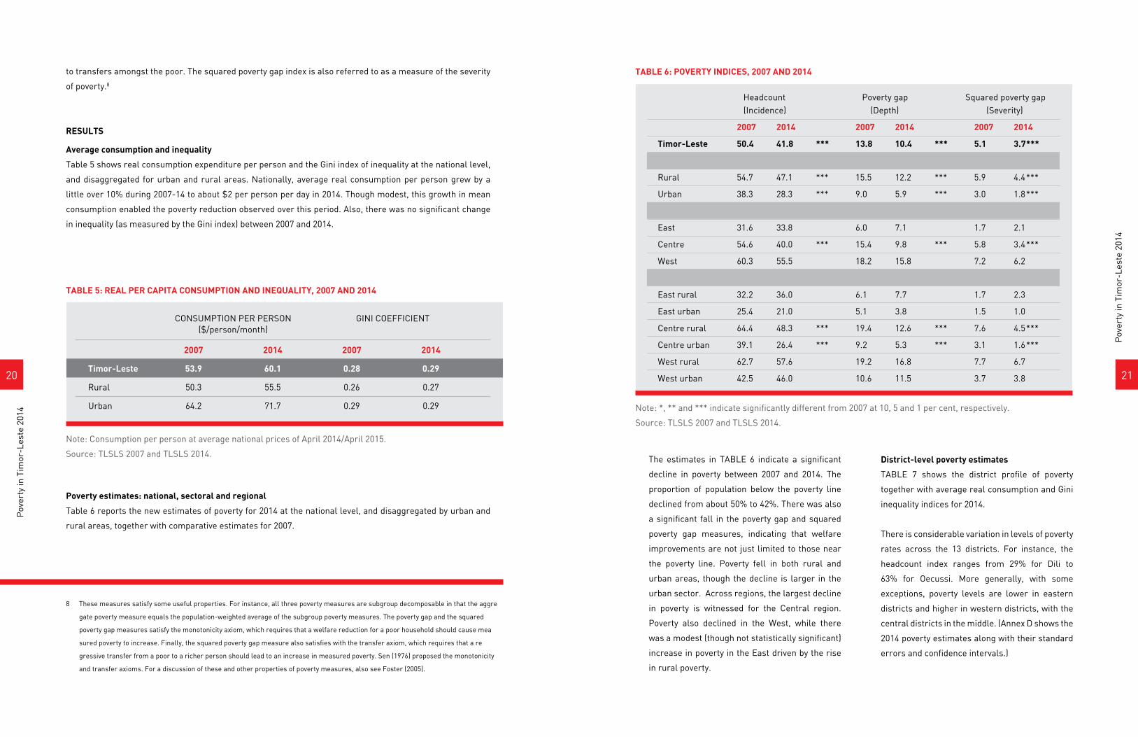
The estimates in TABLE 6 indicate a significant

decline in poverty between 2007 and 2014. The

proportion of population below the poverty line

declined from about 50% to 42%. There was also

a significant fall in the poverty gap and squared

poverty gap measures, indicating that welfare

improvements are not just limited to those near

the poverty line. Poverty fell in both rural and

urban areas, though the decline is larger in the

urban sector. Across regions, the largest decline

in poverty is witnessed for the Central region.

Poverty also declined in the West, while there

was a modest (though not statistically significant)

increase in poverty in the East driven by the rise

in rural poverty.

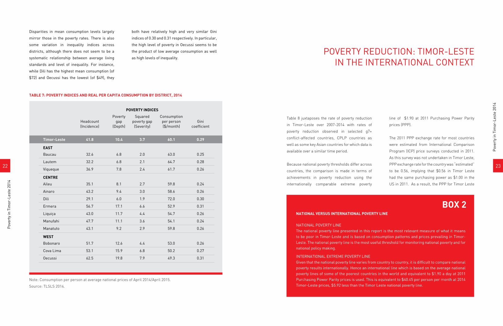
District-level poverty estimates

TABLE 7 shows the district profile of poverty

together with average real consumption and Gini

inequality indices for 2014.

There is considerable variation in levels of poverty

rates across the 13 districts. For instance, the

headcount index ranges from 29% for Dili to

63% for Oecussi. More generally, with some

exceptions, poverty levels are lower in eastern

districts and higher in western districts, with the

central districts in the middle. (Annex D shows the

2014 poverty estimates along with their standard

errors and confidence intervals.)

to transfers amongst the poor. The squared poverty gap index is also referred to as a measure of the severity

of poverty.8

RESULTS

Average consumption and inequality

Table 5 shows real consumption expenditure per person and the Gini index of inequality at the national level,

and disaggregated for urban and rural areas. Nationally, average real consumption per person grew by a

little over 10% during 2007-14 to about $2 per person per day in 2014. Though modest, this growth in mean

consumption enabled the poverty reduction observed over this period. Also, there was no significant change

in inequality (as measured by the Gini index) between 2007 and 2014.

Poverty estimates: national, sectoral and regional

Table 6 reports the new estimates of poverty for 2014 at the national level, and disaggregated by urban and

rural areas, together with comparative estimates for 2007.

8 These measures satisfy some useful properties. For instance, all three poverty measures are subgroup decomposable in that the aggre

gate poverty measure equals the population-weighted average of the subgroup poverty measures. The poverty gap and the squared

poverty gap measures satisfy the monotonicity axiom, which requires that a welfare reduction for a poor household should cause mea

sured poverty to increase. Finally, the squared poverty gap measure also satisfies with the transfer axiom, which requires that a re

gressive transfer from a poor to a richer person should lead to an increase in measured poverty. Sen (1976) proposed the monotonicity

and transfer axioms. For a discussion of these and other properties of poverty measures, also see Foster (2005).

TABLE 5: REAL PER CAPITA CONSUMPTION AND INEQUALITY, 2007 AND 2014

TABLE 6: POVERTY INDICES, 2007 AND 2014

CONSUMPTION PER PERSON GINI COEFFICIENT ($/person/month)

2007 2014 2007 2014

Timor-Leste 53.9 60.1 0.28 0.29

Rural 50.3 55.5 0.26 0.27

Urban 64.2 71.7 0.29 0.29

Note: Consumption per person at average national prices of April 2014/April 2015.

Source: TLSLS 2007 and TLSLS 2014.

Headcount Poverty gap Squared poverty gap (Incidence) (Depth) (Severity)

2007 2014 2007 2014 2007 2014

Timor-Leste 50.4 41.8 *** 13.8 10.4 *** 5.1 3.7 ***

Rural 54.7 47.1 *** 15.5 12.2 *** 5.9 4.4 ***

Urban 38.3 28.3 *** 9.0 5.9 *** 3.0 1.8 ***

East 31.6 33.8 6.0 7.1 1.7 2.1

Centre 54.6 40.0 *** 15.4 9.8 *** 5.8 3.4 ***

West 60.3 55.5 18.2 15.8 7.2 6.2

East rural 32.2 36.0 6.1 7.7 1.7 2.3

East urban 25.4 21.0 5.1 3.8 1.5 1.0

Centre rural 64.4 48.3 *** 19.4 12.6 *** 7.6 4.5 ***

Centre urban 39.1 26.4 *** 9.2 5.3 *** 3.1 1.6 ***

West rural 62.7 57.6 19.2 16.8 7.7 6.7

West urban 42.5 46.0 10.6 11.5 3.7 3.8

Note: *, ** and *** indicate significantly different from 2007 at 10, 5 and 1 per cent, respectively.

Source: TLSLS 2007 and TLSLS 2014.

2322

Pov

erty

in T

imor

-Les

te 2

014

Pov

erty

in T

imor

-Les

te 2

014

Table 8 juxtaposes the rate of poverty reduction

in Timor-Leste over 2007-2014 with rates of

poverty reduction observed in selected g7+

conflict-affected countries, CPLP countries as

well as some key Asian countries for which data is

available over a similar time period.

Because national poverty thresholds differ across

countries, the comparison is made in terms of

achievements in poverty reduction using the

internationally comparable extreme poverty

line of $1.90 at 2011 Purchasing Power Parity

prices (PPP).

The 2011 PPP exchange rate for most countries

were estimated from International Comparison

Program (ICP) price surveys conducted in 2011.

As this survey was not undertaken in Timor Leste,

PPP exchange rate for the country was “estimated”

to be 0.56, implying that $0.56 in Timor Leste

had the same purchasing power as $1.00 in the

US in 2011. As a result, the PPP for Timor Leste

Disparities in mean consumption levels largely

mirror those in the poverty rates. There is also

some variation in inequality indices across

districts, although there does not seem to be a

systematic relationship between average living

standards and level of inequality. For instance,

while Dili has the highest mean consumption (of

$72) and Oecussi has the lowest (of $49), they

both have relatively high and very similar Gini

indices of 0.30 and 0.31 respectively. In particular,

the high level of poverty in Oecussi seems to be

the product of low average consumption as well

as high levels of inequality.

TABLE 7: POVERTY INDICES AND REAL PER CAPITA CONSUMPTION BY DISTRICT, 2014

Note: Consumption per person at average national prices of April 2014/April 2015.

Source: TLSLS 2014.

POVERTY REDUCTION: TIMOR-LESTE IN THE INTERNATIONAL CONTEXT

POVERTY INDICES

Poverty Squared Consumption Headcount gap poverty gap per person Gini (Incidence) (Depth) (Severity) ($/month) coefficient

Timor-Leste 41.8 10.4 3.7 60.1 0.29

EAST

Baucau 32.6 6.8 2.0 63.0 0.25

Lautem 32.2 6.8 2.1 64.7 0.28

Viqueque 36.9 7.8 2.4 61.7 0.26

CENTRE

Aileu 35.1 8.1 2.7 59.8 0.24

Ainaro 43.2 9.4 3.0 58.6 0.26

Dili 29.1 6.0 1.9 72.0 0.30

Ermera 56.7 17.1 6.6 52.9 0.31

Liquiça 43.0 11.7 4.4 54.7 0.26

Manufahi 47.7 11.1 3.6 54.1 0.24

Manatuto 43.1 9.2 2.9 59.8 0.26

WEST

Bobonaro 51.7 12.6 4.4 53.0 0.26

Cova Lima 53.1 15.9 6.8 50.2 0.27

Oecussi 62.5 19.8 7.9 49.3 0.31

NATIONAL VERSUS INTERNATIONAL POVERTY LINE

NATIONAL POVERTY LINEThe national poverty line presented in this report is the most relevant measure of what it means to be poor in Timor-Leste and is based on consumption patterns and prices prevailing in Timor-Leste. The national poverty line is the most useful threshold for monitoring national poverty and for national policy making.

INTERNATIONAL EXTREME POVERTY LINEGiven that the national poverty line varies from country to country, it is difficult to compare national poverty results internationally. Hence an international line which is based on the average national poverty lines of some of the poorest countries in the world and equivalent to $1.90 a day at 2011 Purchasing Power Parity prices is used. This is equivalent to $40.45 per person per month at 2014 Timor-Leste prices, $5.92 less than the Timor Leste national poverty line.

BOX 2

2524

Pov

erty

in T

imor

-Les

te 2

014

Pov

erty

in T

imor

-Les

te 2

014

is less reliable than for other countries where

actual price surveys were conducted. Using the

2011 PPP of 0.56 and after adjusting for inflation

between 2011 and 2014, the international poverty

line in 2014 Timor Leste prices is equivalent to

$1.33 per person or $40.45 per person per month.

This is considerably lower than the 2014 national

poverty line of $46.37 per person per month. It

should therefore be noted that the international

line has less firm grounding than the national

poverty line in the basic need requirements in

Timor Leste. In fact the minimum living standard

is lowered when moving from the national poverty

line to the international poverty line.

Table 8 shows that poverty in Timor-Leste declined

by 16.9 percentage points, from 47.2% in 2007 to

30.3% in 2014. The rate of poverty reduction in

Timor-Leste took place at a more rapid rate than

in Haiti, Sierra Leone, and Togo (among the g7+

countries) as well as China and Indonesia.

TABLE 8: POVERTY REDUCTION IN SELECTED COUNTRIES

Source: TLSLS 2014 and World Bank. Source: TLSLS 2014

Rate of poverty decline at $1.90 (2011 PPP) poverty line

Selected countries Period Average percentage points per year

Selected g7+ countries

Chad 2003-2011 3.1

Congo 2004-2012 1.9

Haiti 2001-2012 0.2

Sierra Leone 2003-2011 0.8

Togo 2006-2011 0.3

Timor Leste 2007-2014 2.4

Selected CPLP countries

Angola 2000-2008 0.3

Mozambique 2002-2008 1.9

Cabo Verde 2001-2007 1.8

Others

China 2002-2010 1.5

Indonesia 2005-2010 0.9

India 2004-2011 2.5

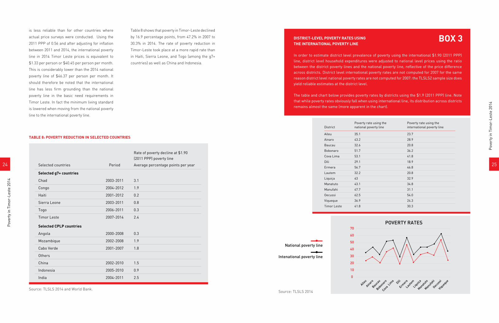
DISTRICT-LEVEL POVERTY RATES USINGTHE INTERNATIONAL POVERTY LINE

In order to estimate district level prevalence of poverty using the international $1.90 (2011 PPP) line, district level household expenditures were adjusted to national level prices using the ratio between the district poverty lines and the national poverty line, reflective of the price difference across districts. District level international poverty rates are not computed for 2007 for the same reason district level national poverty rates are not computed for 2007: the TLSLS2 sample size does yield reliable estimates at the district level.

The table and chart below provides poverty rates by districts using the $1.9 (2011 PPP) line. Note that while poverty rates obviously fall when using international line, its distribution across districts remains almost the same (more apparent in the chart).

BOX 3

Poverty rate using the Poverty rate using theDistrict national poverty line international poverty line

Aileu 35.1 23.7

Ainaro 43.2 28.9

Baucau 32.6 20.8

Bobonaro 51.7 36.2

Cova Lima 53.1 41.8

Dili 29.1 18.9

Ermera 56.7 46.8

Lautem 32.2 20.8

Liquiça 43 32.9

Manatuto 43.1 34.8

Manufahi 47.7 31.1

Oecussi 62.5 54.0

Viqueque 36.9 24.3

Timor Leste 41.8 30.3

POVERTY RATES

Aileu

AinaroBauca

uBobonaro

Cova L

ima

DiliErm

eraLaute

mLiquiça

Manatuto

Manufahi

Oecuss

iViqueque

60

70

50

40

30

20

10

0

National poverty line

Intenational poverty line

2726

Pov

erty

in T

imor

-Les

te 2

014

Pov

erty

in T

imor

-Les

te 2

014

This section investigates the robustness of the

poverty estimates presented above to different

methodological choices. The first subsection

deals with robustness with respect to correcting

for household members’ age and sex in calorie

requirements, the second subsection looks

at changes in the poverty estimates due to

the inclusion of expenses on festivities and

ceremonies in total household consumption, and

the third subsection assesses robustness against

potential biases due to fieldwork team effects. For

brevity, this section presents results pertaining

to the measure of poverty incidence only (the

headcount index); however results for the other

poverty measures (the poverty gap index and the

squared poverty gap index) are similar.

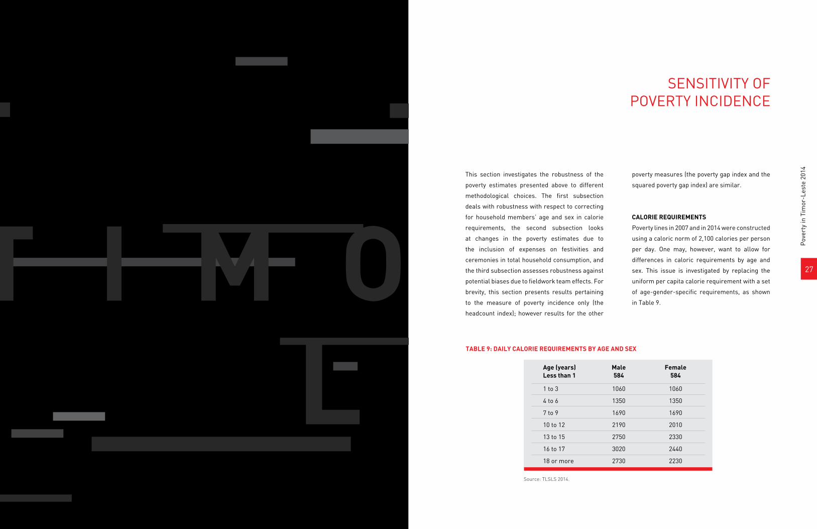
CALORIE REQUIREMENTS

Poverty lines in 2007 and in 2014 were constructed

using a caloric norm of 2,100 calories per person

per day. One may, however, want to allow for

differences in caloric requirements by age and

sex. This issue is investigated by replacing the

uniform per capita calorie requirement with a set

of age-gender-specific requirements, as shown

in Table 9.

SENSITIVITY OFPOVERTY INCIDENCE

TABLE 9: DAILY CALORIE REQUIREMENTS BY AGE AND SEX

Source: TLSLS 2014.

Age (years) Male FemaleLess than 1 584 584

1 to 3 1060 1060

4 to 6 1350 1350

7 to 9 1690 1690

10 to 12 2190 2010

13 to 15 2750 2330

16 to 17 3020 2440

18 or more 2730 2230

P O V

T I M O RL E S T E

E R T Y

2928

Pov

erty

in T

imor

-Les

te 2

014

Pov

erty

in T

imor

-Les

te 2

014

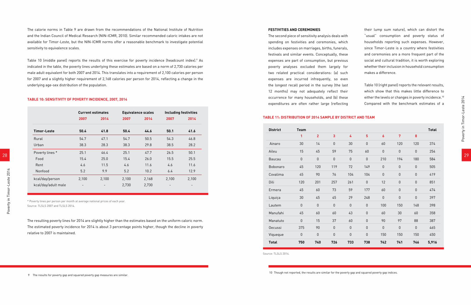
FESTIVITIES AND CEREMONIES

The second piece of sensitivity analysis deals with

spending on festivities and ceremonies, which

includes expenses on marriages, births, funerals,

festivals and similar events. Conceptually, these

expenses are part of consumption, but previous

poverty analyses excluded them largely for

two related practical considerations: (a) such

expenses are incurred infrequently, so even

the longest recall period in the survey (the last

12 months) may not adequately reflect their

occurrence for many households, and (b) these

expenditures are often rather large (reflecting

their lump sum nature), which can distort the

“usual” consumption and poverty status of

households reporting such expenses. However,

since Timor-Leste is a country where festivities

and ceremonies are a more frequent part of the

social and cultural tradition, it is worth exploring

whether their inclusion in household consumption

makes a difference.

Table 10 (right panel) reports the relevant results,

which show that this makes little difference to

either the levels or changes in poverty incidence.10

Compared with the benchmark estimates of a

9 The results for poverty gap and squared poverty gap measures are similar.

The calorie norms in Table 9 are drawn from the recommendations of the National Institute of Nutrition

and the Indian Council of Medical Research (NIN-ICMR, 2010). Similar recommended caloric intakes are not

available for Timor-Leste, but the NIN-ICMR norms offer a reasonable benchmark to investigate potential

sensitivity to equivalence scales.

Table 10 (middle panel) reports the results of this exercise for poverty incidence (headcount index).9 As

indicated in the table, the poverty lines underlying these estimates are based on a norm of 2,730 calories per

male adult equivalent for both 2007 and 2014. This translates into a requirement of 2,100 calories per person

for 2007 and a slightly higher requirement of 2,168 calories per person for 2014, reflecting a change in the

underlying age-sex distribution of the population.

The resulting poverty lines for 2014 are slightly higher than the estimates based on the uniform caloric norm.

The estimated poverty incidence for 2014 is about 3 percentage points higher, though the decline in poverty

relative to 2007 is maintained.

TABLE 10: SENSITIVITY OF POVERTY INCIDENCE, 2007, 2014

TABLE 11: DISTRIBUTION OF 2014 SAMPLE BY DISTRICT AND TEAM Current estimates Equivalence scales Including festivities

2007 2014 2007 2014 2007 2014

Timor-Leste 50.4 41.8 50.4 44.6 50.1 41.6

Rural 54.7 47.1 54.7 50.5 54.3 46.8

Urban 38.3 28.3 38.3 29.8 38.5 28.2

Poverty lines * 25.1 46.4 25.1 47.7 26.5 50.1

Food 15.4 25.0 15.4 26.0 15.5 25.5

Rent 4.6 11.5 4.6 11.6 4.6 11.6

Nonfood 5.2 9.9 5.2 10.2 6.4 12.9

kcal/day/person 2,100 2,100 2,100 2,168 2,100 2,100

kcal/day/adult male - - 2,730 2,730 - -

* Poverty lines per person per month at average national prices of each year.

Source: TLSLS 2007 and TLSLS 2014.

Source: TLSLS 2014.

District Team Total

1 2 3 4 5 6 7 8

Ainaro 30 14 0 30 0 60 120 120 374

Aileu 15 45 59 75 60 0 0 0 254

Baucau 0 0 0 0 0 210 194 180 584

Bobonaro 45 120 119 72 149 0 0 0 505

Covalima 45 90 76 104 104 0 0 0 419

Dili 120 201 257 261 0 12 0 0 851

Ermera 45 60 73 59 177 60 0 0 474

Liquiça 30 45 45 29 248 0 0 0 397

Lautem 0 0 0 0 0 100 150 148 398

Manufahi 45 60 60 43 0 60 30 60 358

Manatuto 0 15 37 60 0 90 97 88 387

Oecussi 375 90 0 0 0 0 0 0 465

Viqueque 0 0 0 0 0 150 150 150 450

Total 750 740 726 733 738 742 741 746 5,916

10 Though not reported, the results are similar for the poverty gap and squared poverty gap indices.

3130

Pov

erty

in T

imor

-Les

te 2

014

Pov

erty

in T

imor

-Les

te 2

014

decline from 50.4% in 2007 to 41.8% in 2014,

these estimates indicate a decline from 50.1%

to 41.6%. The main reason for this small change

is easy to appreciate. The inclusion of festivities

and ceremonies certainly increases non-food and

total consumption of households, but it also raises

the allowance for the non-food component of the

poverty line. Recall that the latter is estimated as

the non-food (excluding rent) expenditure of the

population whose food and rent expenditure is in

the neighbourhood of the food and rent poverty

lines. Thus, effectively, the methodology used for

the estimation of poverty lines offers an element

of built-in stability to the poverty estimates,

which is also reflected in the results reported in

Table 10.

FIELDWORK TEAM EFFECTS

The TLSLS-3 deployed 8 teams to carry out the

entire fieldwork for the yearlong survey. All teams

received the same centralized training prior to

the launch of fieldwork. As noted in Annex A,

for quality assurance purposes, the sample was

randomly distributed across quarters, districts

and teams. Thus, the sample of each district, with

the exception of Oecussi, was randomly allocated

to at least three different teams of fieldworkers

(interpenetrating sampling) whose fieldwork

was spread over the four quarters. Oecussi was

surveyed by two teams, with a different team

visiting each quarter. The distribution of the final

sample by team and district is shown in Table 11.

For a sufficiently large total sample size, the

households surveyed by each team could be

considered an independent random subsample of

the overall sample. However, in smaller samples,

this would only be approximately so, thus raising

the possibility of team effects in finite samples.

Could this bias district-level poverty estimates?

We investigate this by conducting the following

experiment for each team. We consider ignoring

the subsample surveyed by one particular team,

say team j. Thus, the households surveyed by

team j are assigned a sampling weight of zero, and

correspondingly, for each district team j was active

in, the sampling weights of households surveyed

by other teams are increased to achieve the same

total population for the district. Consumption,

poverty lines and poverty measures are then

recalculated for such a reweighted sample,

and then we test for any statistically significant

difference with respect to the benchmark poverty

estimates using the full sample for all teams. The

presence of statistically significant differences

would be suggestive of finite sample biases due

to team effects. The experiment is repeated for

each team j=1,2…8. The results are summarized

in Table 12.11

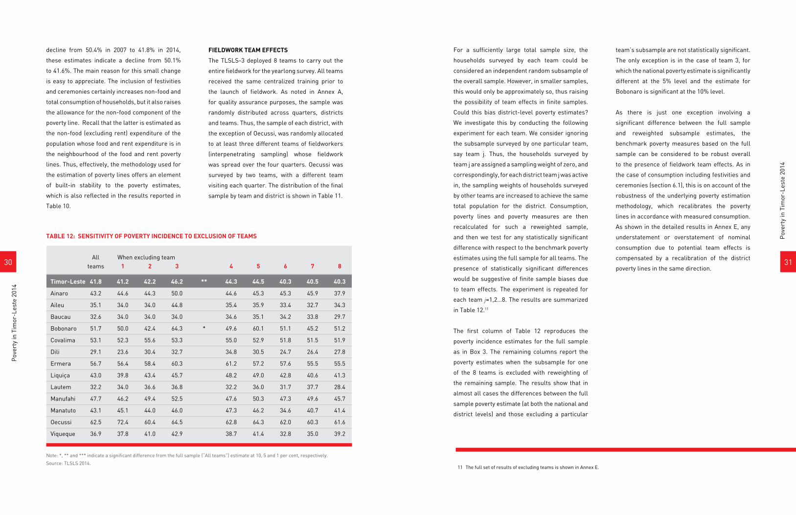
The first column of Table 12 reproduces the

poverty incidence estimates for the full sample

as in Box 3. The remaining columns report the

poverty estimates when the subsample for one

of the 8 teams is excluded with reweighting of

the remaining sample. The results show that in

almost all cases the differences between the full

sample poverty estimate (at both the national and

district levels) and those excluding a particular

team’s subsample are not statistically significant.

The only exception is in the case of team 3, for

which the national poverty estimate is significantly

different at the 5% level and the estimate for

Bobonaro is significant at the 10% level.

As there is just one exception involving a

significant difference between the full sample

and reweighted subsample estimates, the

benchmark poverty measures based on the full

sample can be considered to be robust overall

to the presence of fieldwork team effects. As in

the case of consumption including festivities and

ceremonies (section 6.1), this is on account of the

robustness of the underlying poverty estimation

methodology, which recalibrates the poverty

lines in accordance with measured consumption.

As shown in the detailed results in Annex E, any

understatement or overstatement of nominal

consumption due to potential team effects is

compensated by a recalibration of the district

poverty lines in the same direction.

11 The full set of results of excluding teams is shown in Annex E.

TABLE 12: SENSITIVITY OF POVERTY INCIDENCE TO EXCLUSION OF TEAMS

Note: *, ** and *** indicate a significant difference from the full sample (“All teams”) estimate at 10, 5 and 1 per cent, respectively.

Source: TLSLS 2014.

All When excluding team teams 1 2 3 4 5 6 7 8

Timor-Leste 41.8 41.2 42.2 46.2 ** 44.3 44.5 40.3 40.5 40.3

Ainaro 43.2 44.6 44.3 50.0 44.6 45.3 45.3 45.9 37.9

Aileu 35.1 34.0 34.0 44.8 35.4 35.9 33.4 32.7 34.3

Baucau 32.6 34.0 34.0 34.0 34.6 35.1 34.2 33.8 29.7

Bobonaro 51.7 50.0 42.4 64.3 * 49.6 60.1 51.1 45.2 51.2

Covalima 53.1 52.3 55.6 53.3 55.0 52.9 51.8 51.5 51.9

Dili 29.1 23.6 30.4 32.7 34.8 30.5 24.7 26.4 27.8

Ermera 56.7 56.4 58.4 60.3 61.2 57.2 57.6 55.5 55.5

Liquiça 43.0 39.8 43.4 45.7 48.2 49.0 42.8 40.6 41.3

Lautem 32.2 34.0 36.6 36.8 32.2 36.0 31.7 37.7 28.4

Manufahi 47.7 46.2 49.4 52.5 47.6 50.3 47.3 49.6 45.7

Manatuto 43.1 45.1 44.0 46.0 47.3 46.2 34.6 40.7 41.4

Oecussi 62.5 72.4 60.4 64.5 62.8 64.3 62.0 60.3 61.6

Viqueque 36.9 37.8 41.0 42.9 38.7 41.4 32.8 35.0 39.2

3332

Pov

erty

in T

imor

-Les

te 2

014

Pov

erty

in T

imor

-Les

te 2

014

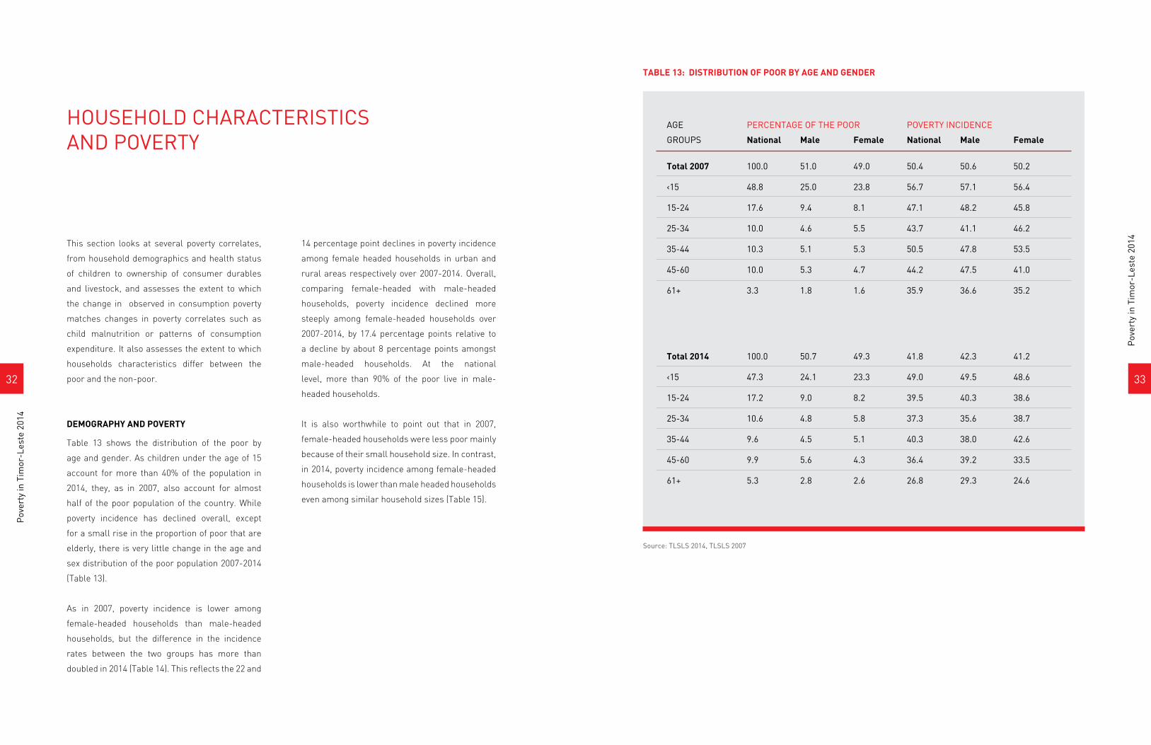
This section looks at several poverty correlates,

from household demographics and health status

of children to ownership of consumer durables

and livestock, and assesses the extent to which

the change in observed in consumption poverty

matches changes in poverty correlates such as

child malnutrition or patterns of consumption

expenditure. It also assesses the extent to which

households characteristics differ between the

poor and the non-poor.

DEMOGRAPHY AND POVERTY

Table 13 shows the distribution of the poor by

age and gender. As children under the age of 15

account for more than 40% of the population in

2014, they, as in 2007, also account for almost

half of the poor population of the country. While

poverty incidence has declined overall, except

for a small rise in the proportion of poor that are

elderly, there is very little change in the age and

sex distribution of the poor population 2007-2014

(Table 13).

As in 2007, poverty incidence is lower among

female-headed households than male-headed

households, but the difference in the incidence

rates between the two groups has more than

doubled in 2014 (Table 14). This reflects the 22 and

14 percentage point declines in poverty incidence

among female headed households in urban and

rural areas respectively over 2007-2014. Overall,

comparing female-headed with male-headed

households, poverty incidence declined more

steeply among female-headed households over

2007-2014, by 17.4 percentage points relative to

a decline by about 8 percentage points amongst

male-headed households. At the national

level, more than 90% of the poor live in male-

headed households.

It is also worthwhile to point out that in 2007,

female-headed households were less poor mainly

because of their small household size. In contrast,

in 2014, poverty incidence among female-headed

households is lower than male headed households

even among similar household sizes (Table 15).

HOUSEHOLD CHARACTERISTICSAND POVERTY

TABLE 13: DISTRIBUTION OF POOR BY AGE AND GENDER

Source: TLSLS 2014, TLSLS 2007

AGE PERCENTAGE OF THE POOR POVERTY INCIDENCE

GROUPS National Male Female National Male Female

Total 2007 100.0 51.0 49.0 50.4 50.6 50.2

‹15 48.8 25.0 23.8 56.7 57.1 56.4

15-24 17.6 9.4 8.1 47.1 48.2 45.8

25-34 10.0 4.6 5.5 43.7 41.1 46.2

35-44 10.3 5.1 5.3 50.5 47.8 53.5

45-60 10.0 5.3 4.7 44.2 47.5 41.0

61+ 3.3 1.8 1.6 35.9 36.6 35.2

Total 2014 100.0 50.7 49.3 41.8 42.3 41.2

‹15 47.3 24.1 23.3 49.0 49.5 48.6

15-24 17.2 9.0 8.2 39.5 40.3 38.6

25-34 10.6 4.8 5.8 37.3 35.6 38.7

35-44 9.6 4.5 5.1 40.3 38.0 42.6

45-60 9.9 5.6 4.3 36.4 39.2 33.5

61+ 5.3 2.8 2.6 26.8 29.3 24.6

3534

Pov

erty

in T

imor

-Les

te 2

014

Pov

erty

in T

imor

-Les

te 2

014

CONSUMPTION PATTERN AND POVERTY

Table 16 shows the share of major consumption

categories in total consumption. The share of

food in total consumption expenditure declined

from 66% to 54% over 2007-2014. Not only that,

the decline was larger for the poor (14 percentage

points) than for the non-poor (11 percentage

points). However, the most significant change

was in the share of rental expenditures, especially

for the poor: rental share more than doubled from

12.6% in 2007 to 27.2% in 2014. Share of non-food

expenditures increased marginally for both poor

and non-poor while shares of utilities, health, and

education declined.

NUTRITIONAL STATUS OF CHILDREN

Table 17 provides information on the nutritional

status of children based on anthropometric

measurements. It is clear that both the incidence

of underweight children (weight lower than that of

a reference child of a particular age) and wasting

(weight lower than that of a reference child of a

particular height) decreased significantly over

2007-2014. The incidence of wasting almost

halved while the incidence of underweight children

declined by about 16 percentage points indicating

a substantial decline in acute malnutrition among

children. However such rates of progress are

not observed for stunting (height lower than that

of a reference child of a particular age) where

the decline was only about 5 percentage points.

The stunting prevalence rate itself remains high

at 49.2% implying that about half the children

in the country continue to suffer from chronic

malnutrition, most likely due to inadequate intake

of essential micronutrients.

OWNERSHIP OF LIVESTOCK AND OTHER

DURABLE GOODS

There are some noticeable changes in ownership

of consumer durables between 2007 and 2014. As

Table18 shows, ownership of mobile phones and

TABLE 14: POVERTY AMONGST FEMALE AND MALE-HEADED HOUSEHOLDS

TABLE 15. POVERTY AMONGST FEMALE AND MALE-HEADED HOUSEHOLDS BY HOUSEHOLD SIZE

TABLE 16: SHARES OF MAJOR CONSUMPTION CATEGORIES IN TOTAL CONSUMPTION, BY POVERTY STATUS

POVERTY INCIDENCE (%) PERCENTAGE OF THE POOR

National Rural Urban National Rural Urban

Total 2007 50.4 54.7 38.3 100.0 100.0 100.0

Female-headed 45.0 47.2 39.2 9.0 8.6 10.9

Male-headed 51.0 55.5 38.2 91.0 91.4 89.1

Total 2014 41.8 47.1 28.3 100.0 100.0 100.0

Female-headed 27.6 32.8 16.9 6.9 6.9 7.3

Male-headed 43.4 48.6 29.9 93.1 93.2 92.7

%

HOUSEHOLD POVERTY INCIDENCE

SIZE National Male Female

Total 2007 50.4 51.0 45.0

1 or 2 8.1 6.4 10.5

3 20.4 17.8 26.8

4 32.4 31.9 36.2

5 43.8 42.5 53.1

6 53.6 53.0 61.4

7+ 61.6 61.4 64.9

Total 2014 41.8 43.4 27.6

1 or 2 1.4 1.7 0.8

3 11.5 13.2 6.1

4 22.7 22.6 23.6

5 27.5 27.4 28.0

6 43.8 44.2 39.8

7+ 56.2 57.1 43.4

(%)

2007 2014

National Non-poor Poor National Non-poor Poor

Total 100.0 100.0 100.0 100.0 100.0 100.0

Food 66.2 64.3 70.6 54.0 53.1 57.0

Non-food 10.4 11.4 8.2 12.9 14.1 9.2

Utilities 8.7 9.4 7.0 8.0 8.6 5.9

Rent 12.7 12.8 12.6 24.2 23.2 27.2

Health 0.6 0.6 0.4 0.2 0.2 0.2

Education 1.4 1.5 1.1 0.7 0.7 0.6

Source: TLSLS 2014

Source: TLSLS 2014Source: TLSLS 2014

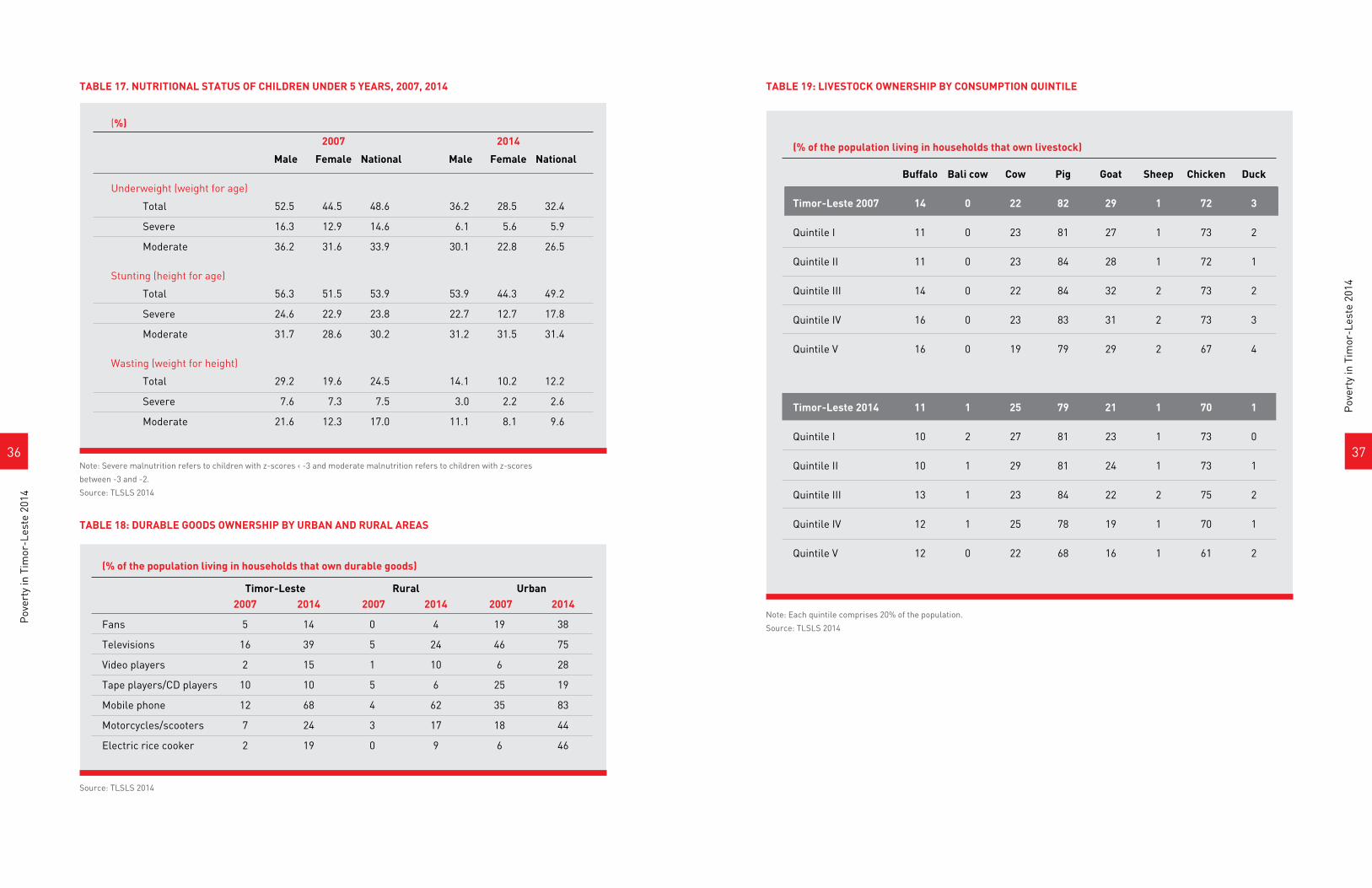
3736

Pov

erty

in T

imor

-Les

te 2

014

Pov

erty

in T

imor

-Les

te 2

014

TABLE 17. NUTRITIONAL STATUS OF CHILDREN UNDER 5 YEARS, 2007, 2014

TABLE 18: DURABLE GOODS OWNERSHIP BY URBAN AND RURAL AREAS

TABLE 19: LIVESTOCK OWNERSHIP BY CONSUMPTION QUINTILE

Note: Severe malnutrition refers to children with z-scores ‹ -3 and moderate malnutrition refers to children with z-scores

between -3 and -2.

Source: TLSLS 2014

(%)

2007 2014

Male Female National Male Female National

Underweight (weight for age)

Total 52.5 44.5 48.6 36.2 28.5 32.4

Severe 16.3 12.9 14.6 6.1 5.6 5.9

Moderate 36.2 31.6 33.9 30.1 22.8 26.5

Stunting (height for age)

Total 56.3 51.5 53.9 53.9 44.3 49.2

Severe 24.6 22.9 23.8 22.7 12.7 17.8

Moderate 31.7 28.6 30.2 31.2 31.5 31.4

Wasting (weight for height)

Total 29.2 19.6 24.5 14.1 10.2 12.2

Severe 7.6 7.3 7.5 3.0 2.2 2.6

Moderate 21.6 12.3 17.0 11.1 8.1 9.6

(% of the population living in households that own durable goods)

Timor-Leste Rural Urban 2007 2014 2007 2014 2007 2014

Fans 5 14 0 4 19 38

Televisions 16 39 5 24 46 75

Video players 2 15 1 10 6 28

Tape players/CD players 10 10 5 6 25 19

Mobile phone 12 68 4 62 35 83

Motorcycles/scooters 7 24 3 17 18 44

Electric rice cooker 2 19 0 9 6 46

Note: Each quintile comprises 20% of the population.

Source: TLSLS 2014

(% of the population living in households that own livestock)

Buffalo Bali cow Cow Pig Goat Sheep Chicken Duck

Timor-Leste 2007 14 0 22 82 29 1 72 3

Quintile I 11 0 23 81 27 1 73 2

Quintile II 11 0 23 84 28 1 72 1

Quintile III 14 0 22 84 32 2 73 2

Quintile IV 16 0 23 83 31 2 73 3

Quintile V 16 0 19 79 29 2 67 4

Timor-Leste 2014 11 1 25 79 21 1 70 1

Quintile I 10 2 27 81 23 1 73 0

Quintile II 10 1 29 81 24 1 73 1

Quintile III 13 1 23 84 22 2 75 2

Quintile IV 12 1 25 78 19 1 70 1

Quintile V 12 0 22 68 16 1 61 2

Source: TLSLS 2014

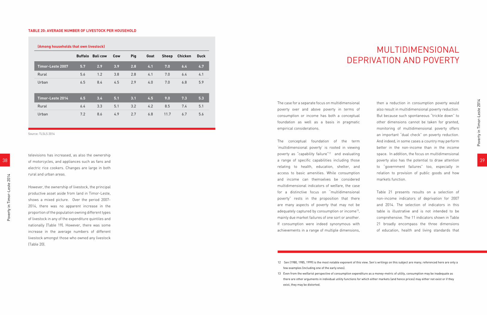
3938

Pov

erty

in T

imor

-Les

te 2

014

Pov

erty

in T

imor

-Les

te 2

014

The case for a separate focus on multidimensional

poverty over and above poverty in terms of

consumption or income has both a conceptual

foundation as well as a basis in pragmatic

empirical considerations.

The conceptual foundation of the term

‘multidimensional poverty’ is rooted in viewing

poverty as “capability failure”12 and evaluating

a range of specific capabilities including those

relating to health, education, shelter, and

access to basic amenities. While consumption

and income can themselves be considered

multidimensional indicators of welfare, the case

for a distinctive focus on “multidimensional

poverty” rests in the proposition that there

are many aspects of poverty that may not be

adequately captured by consumption or income13,

mainly due market failures of one sort or another.

If consumption were indeed synonymous with

achievements in a range of multiple dimensions,

then a reduction in consumption poverty would

also result in multidimensional poverty reduction.

But because such spontaneous “trickle down” to

other dimensions cannot be taken for granted,

monitoring of multidimensional poverty offers

an important “dual check” on poverty reduction.

And indeed, in some cases a country may perform

better in the non-income than in the income

space. In addition, the focus on multidimensional

poverty also has the potential to draw attention

to “government failures” too, especially in

relation to provision of public goods and how

markets function.

Table 21 presents results on a selection of

non-income indicators of deprivation for 2007

and 2014. The selection of indicators in this

table is illustrative and is not intended to be

comprehensive. The 11 indicators shown in Table

21 broadly encompass the three dimensions

of education, health and living standards that

MULTIDIMENSIONALDEPRIVATION AND POVERTY

12 Sen (1980, 1985, 1999) is the most notable exponent of this view. Sen’s writings on this subject are many; referenced here are only a

few examples (including one of the early ones).

13 Even from the welfarist perspective of consumption expenditure as a money-metric of utility, consumption may be inadequate as

there are other arguments in individual utility functions for which either markets (and hence prices) may either not exist or if they

exist, they may be distorted.

TABLE 20: AVERAGE NUMBER OF LIVESTOCK PER HOUSEHOLD

televisions has increased, as also the ownership

of motorcycles, and appliances such as fans and

electric rice cookers. Changes are large in both

rural and urban areas.

However, the ownership of livestock, the principal

productive asset aside from land in Timor-Leste,

shows a mixed picture. Over the period 2007-

2014, there was no apparent increase in the

proportion of the population owning different types

of livestock in any of the expenditure quintiles and

nationally (Table 19). However, there was some

increase in the average numbers of different

livestock amongst those who owned any livestock

(Table 20).

(Among households that own livestock)

Buffalo Bali cow Cow Pig Goat Sheep Chicken Duck

Timor-Leste 2007 5.7 2.9 3.9 2.8 4.1 7.0 6.4 4.7

Rural 5.6 1.2 3.8 2.8 4.1 7.0 6.4 4.1

Urban 6.5 8.4 4.5 2.9 4.0 7.0 6.8 5.9

Timor-Leste 2014 6.5 3.4 5.1 3.1 4.5 9.0 7.3 5.3

Rural 6.4 3.3 5.1 3.2 4.2 8.5 7.4 5.1

Urban 7.2 8.6 4.9 2.7 6.8 11.7 6.7 5.6

Source: TLSLS 2014

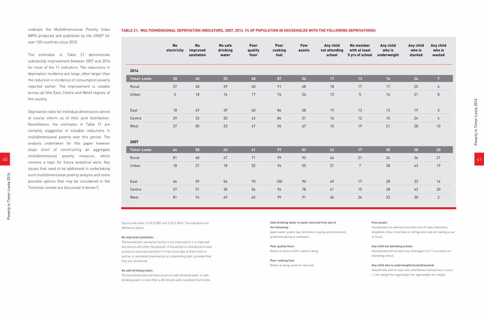
4140

Pov

erty

in T

imor

-Les

te 2

014

Pov

erty

in T

imor

-Les

te 2

014

underpin the Multidimensional Poverty Index

(MPI) produced and published by the UNDP for

over 100 countries since 2010.

The estimates in Table 21 demonstrate

substantial improvement between 2007 and 2014

for most of the 11 indicators. The reductions in

deprivation incidence are large, often larger than

the reduction in incidence of consumption poverty

reported earlier. The improvement is notable

across all (the East, Centre and West) regions of

the country.

Deprivation rates for individual dimensions cannot

of course inform us of their joint distribution.

Nonetheless, the estimates in Table 21 are

certainly suggestive of sizeable reductions in

multidimensional poverty over this period. The

analysis undertaken for this paper however

stops short of constructing an aggregate

multidimensional poverty measure, which

remains a topic for future analytical work. Key

issues that need to be addressed in undertaking

such multidimensional poverty analysis and some

possible options that may be considered in the

Timorese context are discussed in Annex F.

TABLE 21: MULTIDIMENSIONAL DEPRIVATION INDICATORS, 2007, 2014 (% OF POPULATION IN HOUSEHOLDS WITH THE FOLLOWING DEPRIVATIONS)

Source and notes: TLSLS 2007 and TLSLS 2014. The indicators are

defined as below.

No improved sanitation:

The household’s sanitation facility is not improved or it is improved

but shared with other households. A household is considered to have

access to improved sanitation if it has some type of flush toilet or

latrine, or ventilated improved pit or composting toilet, provided that

they are not shared.

No safe drinking water:

The household does not have access to safe drinking water or safe

drinking water is more than a 30-minute walk roundtrip from home.

No No No safe Poor Poor Few Any child No member Any child Any child Any child electricity improved drinking quality cooking assets not attending with at least who is who is who is sanitation water floor fuel school 5 yrs of school underweight stunted wasted

2014

Timor-Leste 28 40 25 48 87 56 17 13 16 24 7

Rural 37 48 29 60 91 68 18 17 17 25 6

Urban 3 18 16 17 76 24 12 5 14 21 8

East 18 49 39 60 86 58 19 13 13 19 5

Centre 29 32 20 43 84 51 16 12 15 24 6

West 37 50 23 47 96 67 15 19 21 28 10

2007

Timor-Leste 64 58 40 61 97 83 42 17 35 38 20

Rural 81 68 47 71 99 93 46 21 34 36 21

Urban 18 27 18 32 94 55 31 7 38 43 19

East 66 59 54 70 100 90 49 17 28 33 14

Centre 57 51 30 56 96 78 41 15 38 43 20

West 81 74 49 63 99 91 36 24 33 30 2

Safe drinking water is water sourced from any of

the following:

piped water, public tap, borehole or pump, protected well,

protected spring or rainwater.

Poor quality floor:

Refers to floors of dirt, sand or dung.

Poor cooking fuel:

Refers to dung, wood or charcoal.

Few assets:

Households not owning more than one of radio, television,

telephone, bike, motorbike or refrigerator and not owning a car

or truck.

Any child not attending school:

Households with at least one child aged 6 to 11 currently not

attending school.

Any child who is underweight/stunted/wasted:

Households with at least one child below 5 whose has z-score

‹-2 for weight-for-age/height-for-age/weight-for-height.

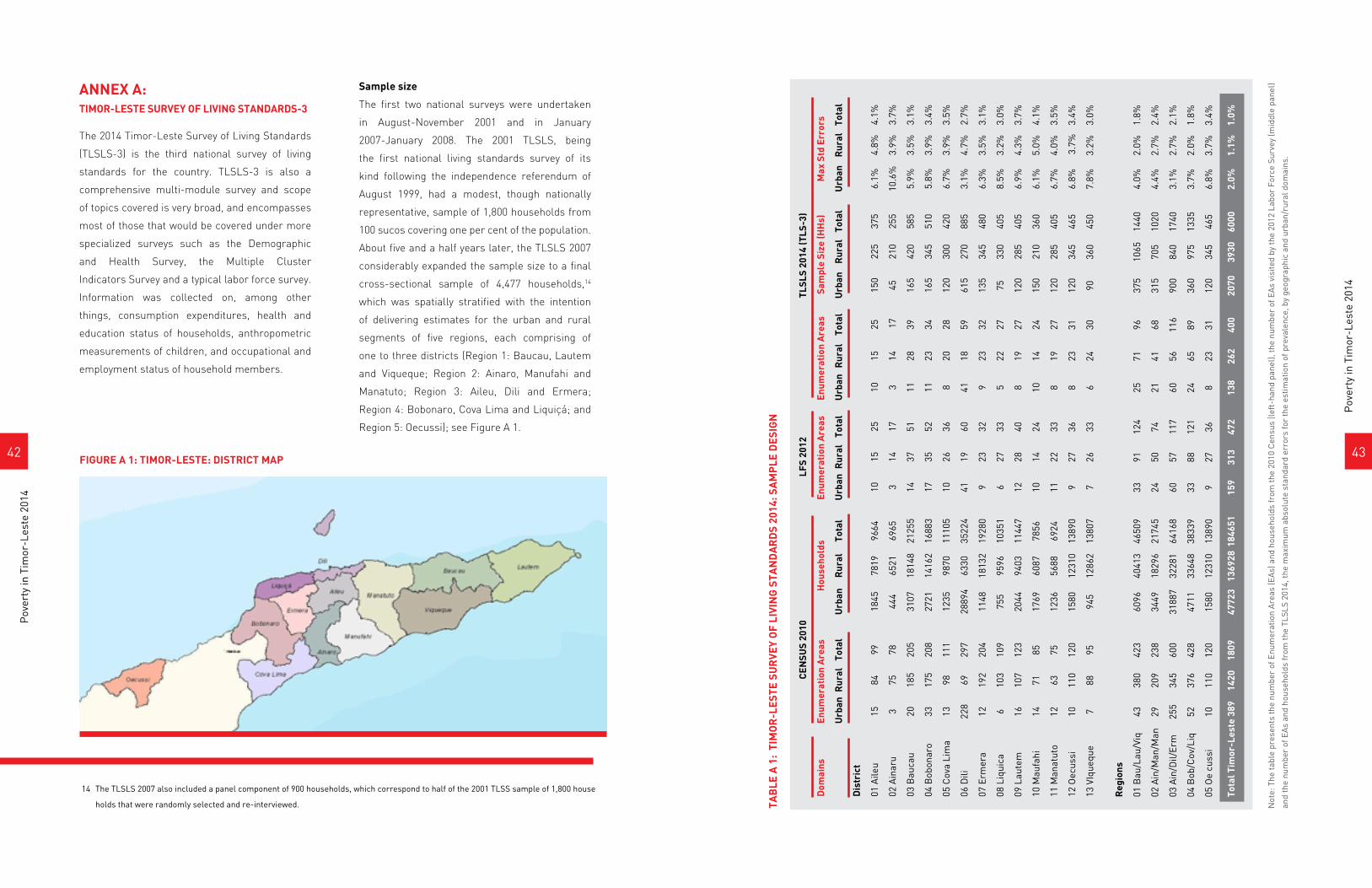
4342

Pov

erty

in T

imor

-Les

te 2

014

Pov

erty

in T

imor

-Les

te 2

014

ANNEX A:TIMOR-LESTE SURVEY OF LIVING STANDARDS-3

The 2014 Timor-Leste Survey of Living Standards

(TLSLS-3) is the third national survey of living

standards for the country. TLSLS-3 is also a

comprehensive multi-module survey and scope

of topics covered is very broad, and encompasses

most of those that would be covered under more

specialized surveys such as the Demographic

and Health Survey, the Multiple Cluster

Indicators Survey and a typical labor force survey.

Information was collected on, among other

things, consumption expenditures, health and

education status of households, anthropometric

measurements of children, and occupational and

employment status of household members.

Sample size

The first two national surveys were undertaken

in August-November 2001 and in January

2007-January 2008. The 2001 TLSLS, being

the first national living standards survey of its

kind following the independence referendum of

August 1999, had a modest, though nationally

representative, sample of 1,800 households from

100 sucos covering one per cent of the population.

About five and a half years later, the TLSLS 2007

considerably expanded the sample size to a final

cross-sectional sample of 4,477 households,14

which was spatially stratified with the intention

of delivering estimates for the urban and rural

segments of five regions, each comprising of

one to three districts (Region 1: Baucau, Lautem

and Viqueque; Region 2: Ainaro, Manufahi and

Manatuto; Region 3: Aileu, Dili and Ermera;

Region 4: Bobonaro, Cova Lima and Liquiçá; and

Region 5: Oecussi); see Figure A 1.

14 The TLSLS 2007 also included a panel component of 900 households, which correspond to half of the 2001 TLSS sample of 1,800 house

holds that were randomly selected and re-interviewed.

FIGURE A 1: TIMOR-LESTE: DISTRICT MAP

TAB

LE A

1:

TIM

OR

-LES

TE S

UR

VEY

OF

LIVI

NG

STA

ND

AR

DS

2014

: SA

MP

LE D

ESIG

N

CEN

SUS

2010

LF

S 20

12

TL

SLS

2014

(TLS

-3)

Dom

ains

E

num

erat

ion

Are

as

H

ouse

hold

s

E

num

erat

ion

Are

as

E

num

erat

ion

Are

as

Sam

ple

Size

(HH

s)

Max

Std

Err

ors

U

rban

Rur

al

Tota

l U

rban

R

ural

To

tal

Urb

an R

ural

To

tal

Urb

an

Rur

al

Tota

l U

rban

R

ural

To

tal

Urb

an

Rur

al

Tota

l

Dis

tric

t

01 A

ileu

15

84

99

1845

78

19

9664

10

15

25

10

15

25

15

0 22

5 37

5 6.

1%

4.8%

4.

1%

02 A

inar

u 3

75

78

444

6521

69

65

3 14

17

3

14

17

45

21

0

255

10

.6%

3.

9%

3.7%

03 B

auca

u

20

185

20

5

3107

18

148

21

255

14

37

51

11

28

39

165

42

0

585

5.

9%

3.5%

3.

1%

04 B

obon

aro

33

175

208

2721

14

162

1688

3 17

35

52

11

23

34

16

5

345

510

5.

8%

3.9%

3.

4%

05 C

ova

Lim

a

13

98

111

1235

98

70

1110

5 10

26

36

8

20

28

120

300

420

6.

7%

3.9%

3.

5%

06 D

ili

228

69

297

2889

4 63

30

3522

4 41

19

60

41

18

59

61

5 27

0 88

5 3.

1%

4.7%

2.

7%

07 E

rmer

a

12

192

204

1148

18

132

1928

0 9

23

32

9 23

32

13

5 34

5 48

0 6.

3%

3.5%

3.

1%

08 L

iqui

ca

6 10

3 10

9 75

5 95

96

1035

1 6

27

33

5 22

27

75

33

0 40

5

8.5%

3.

2%

3.0%

09 L

aute

m

16

107

123

2044

94

03

1144

7 12

28

40

8

19

27

120

28

5 40

5 6.

9%

4.3%

3.

7%

10 M

aufa

hi

14

71

85

1769

60

87

7856

10

14

24

10

14

24

15

0 21

0 36

0 6.

1%

5.0%

4.

1%

11 M

anat

uto

12

63

75

12

36

5688

69

24

11

22

33

8 19

27

12

0 28

5 40

5 6.

7%

4.0%

3.

5%

12 O

ecus

si

10

110

12

0 15

80

1231

0

1389

0 9

27

36

8 23

31

12

0 34

5 46

5 6.

8%

3.7

%

3.4%

13 V

Ique

que

7

88

95

945

1286

2 13

807

7 26

33

6

24

30

90

360

45

0 7.

8%

3.2%

3.

0%

Reg

ions

01 B

au/L

au/V

iq

43

380

423

6096

40

413

4650

9 33

91

12

4 25

71

96

37

5 10

65

1440

4.

0%

2.0%

1.

8%

02 A

in/M

an/M

an

29

209

238

3449

18

296

2174

5 24

50

74

21

41

68

31

5 70

5 10

20

4.4%

2.

7%

2.4%

03 A

in/D

il/Er

m

255

345

600

3188

7 32

281

6416

8 60

57

11

7 60

56

11

6 90

0 84

0 17

40

3.1%

2.

7%

2.1%

04 B

ob/C

ov/L

iq

52

376

428

4711

33

648

3833

9 33

88

12

1 24

65

89

36

0 97

5 13

35

3.7%

2.

0%

1.8%

05 O

e cu

ssi

10

110

120

1580

12

310

1389

0 9

27

36

8 23

31

12

0 34

5 46

5 6.

8%

3.7%

3.

4%

Tota

l Tim

or-L

este

389

14

20

1809

47

723

1369

28 1

8465

1 15

9 31

3 47

2 13

8 26

2

400

2070

39

30

6000

2.

0%

1.1%

1.

0%

Not

e: T

he ta

ble

pres

ents

the

num

ber

of E

num

erat

ion

Are

as (E

As)

and

hou

seho

lds

from

the

2010

Cen

sus

(left

-han

d pa

nel),

the

num

ber

of E

As

visi

ted

by th

e 20

12 L

abor

For

ce S

urve

y (m

iddl

e pa

nel)

and

the

num

ber

of E

As

and

hous

ehol

ds fr

om th

e TL

SLS

2014

, the

max

imum

abs

olut

e st

anda

rd e

rror

s fo

r th

e es

timat

ion

of p

reva

lenc

e, b

y ge

ogra

phic

and

urb

an/r

ural

dom

ains

.

4544

Pov

erty

in T

imor

-Les

te 2

014

Pov

erty

in T

imor

-Les

te 2

014

responsible for 50 EAs and visited one enumeration

area per week. Each enumerator within the team

was responsible for interviewing 5 households,

with the enumeration of each household spread

over four visits.

The data for each PSU were transmitted on a

continuous basis to the Directorate General of

Statistics (DGE) Office in Dili. The transfer was

done through the internet using USB-modems.

Data quality control

Three layers of supervision were utilized to assure

high data quality of the TLSLS 2014:

1. Human supervision. This layer consists of

(i) team supervisors re-visiting some randomly

selected households to ask selected questions

again; (ii) the core team from the DGE re-visiting

some households to supervise the supervisors.

The DGE prepared standard supervision forms

that were used for this purpose.

2. Computer-based quality controls. This

second layer of supervision involved the

data entry program that complemented human

supervision, applying consistency checks

to each households’ data. The information

registered on the questionnaires was

immediately entered into laptops, using an

“intelligent” data entry program that allows

for both data entry and consistency checks.

Possible inconsistencies were resolved

by asking the household members the same

questions again, during the next visit. Teams

did not move to another enumeration area

until all inconsistencies were resolved in all of

the 15 questionnaires.

Examples of the multiple consistency checks

included in the data entry program are: (1)

checking that the per capita calorie intake

of each household (as reported by the food

consumption sections of the questionnaire)

is within a reasonable range for the

household’s composition (the distribution of

household members by age and sex), (2)

checking for the consistency of each child’s

anthropometric measures (weight and height),

using the World Health Organization

reference tables.

3. Monitoring selected indicators. As there is

perverse incentive for the interviewers to

modify some answers to reduce work, the third

layer of data quality control involved DGE Office

in Dili monitoring the evolution of several

indicators using partial national databases,

periodically received from the field. Some

examples of the indicators monitored were

average household size, average number

of food items consumed, average number

of children under five, and average number of

women between 15-49 years that can be

expected to remain similar all four quarters of

the survey and across teams.

ANNEX B:CONSUMPTION-BASED WELFARE INDICATOR

Two key elements of poverty measurement

relate to (i) the construction of an individual

welfare indicator, and (ii) the construction of an

appropriate poverty line against which the chosen

welfare indicator will be compared in order to

classify individuals as poor or non-poor, and if

poor, to measure their consumption shortfalls

(relative to the poverty line) . This Annex describes

the procedures adopted in relation to the

first element.

With an expansion of statistical capacity within

the country as well as a maturing of government

institutions and operations, greater demands were

placed on the third round of the living standards

survey. The TLSLS 2014 faced the challenge of

delivering estimates of comparable quality for

each of Timor-Leste’s 13 districts, leading to a

further expansion of the sample size. To meet this

challenge within the existing resource and time

constraints, it was decided not to have a panel

component in the TLSLS 2014, but to augment

the total sample size to 6,000 households with 15

sample households in each of 400 enumeration

areas (EAs) stratified across rural and urban

sectors of the 13 districts.

Sample design

The TLSLS 2014 sample was selected in two

stages: Census Enumeration Areas (EAs) as

Primary Sampling Units (PSUs) and individual

households as secondary units. A cluster of 15

households was visited in each PSU.

The sample frame for TLSLS 2014 makes use

of the recent 2010 Census, but indirectly, taking

advantage of the household listings prepared for

the Labor Force Survey (LFS) in 2012. The LFS

distributed its sample of 472 EAs across the urban

and rural segments of the 13 districts, with an

allocation that was considered adequate for the

TLSLS 2014.

The TLSLS 2014 only needed to visit a subsample

of 400 out of the 472 EAs for the LFS. The TLSLS

2014 subsample was allocated to the same strata

as the LFS, and the 400 PSUs were randomly

selected with equal probabilities within each

stratum. The detailed sample design is shown in

Table A1.

The right-hand panel of Table A1 above presents

the sample size and the maximum absolute

standard errors of the TLSLS 2014, by district and

urban/rural domains. The left-hand panel shows

the number of EAs and households of the 2010

Census, and the number of EAs visited by the LFS.

The figures are broken down by district on top,

and according to the regions used by the TLSLS

2007 (TLSLS-2) at the bottom.

The standard errors for most indicators of

interest will be between 3 and 4 percentage

points at the district level, but larger for the

urban/rural subdivisions of each district. In other

words, the survey can be expected to allow basic

comparisons between districts, but not for the

urban/rural portions of each district. Urban/rural

comparisons would be possible at the national

level and marginally possible within the five

regions used by the TLSLS-2.

Like its predecessor, the TLSLS 2014 was fielded

over a yearlong period and the sample was

randomly distributed across the four quarters

of the year to capture seasonality. For quality

assurance purposes, the sample of each district

was also randomly allocated to at least three

different teams of fieldworkers (interpenetrating

sampling). The two criteria (random allocation

into quarters and teams) could be satisfied

simultaneously in all districts except Oecussi,

which was visited by a different team each quarter.

Fieldwork organization and data management

The fieldwork organization for the TLSLS 2014 is

similar to that used successfully for the TLSLS-2

in 2007. The fieldworkers were organized into

8 independent teams, each of them composed

of one supervisor, three enumerators, one data

entry operator and one driver. Each team was

4746

Pov

erty

in T

imor

-Les

te 2

014

Pov

erty

in T

imor

-Les

te 2

014

The general principle followed was to (a) to exclude

items that do not directly contribute to household

consumption, (b) to exclude items that are lumpy

and highly infrequent in nature. Following this

principle, expenses related to taxes, festivities

and ceremonies, jewelry, furniture, household

equipment and other durables, donations,

gambling/cash losses and bank deposits, were

excluded: 21 non-food items in 2007 and 20 non-

food items in 2014 (deposits on savings accounts

no longer needed to be excluded in 2014 because

this non-food item was not included in the

questionnaire). Altogether, 52 non-food items in

2007 and 53 non-food items in 2014 were included

in the measure of household consumption. The

additional item in 2014 relating to mobile phone

expenses was largely irrelevant for 2007 because

of the very limited usage of mobile phones at

that time.

Reference period

As for the reference period, the TLSLS-2 captures

non-food consumption using two reference

periods: the last month and the last 12 months.

The chosen reference period is the last month.

However, households do not buy many non-food

items every month. In order to better capture the

overall non-food consumption of the population,

whenever households do not purchase a non-food

item in the last month but report its consumption

in the last 12 months, the latter is converted to a

monthly basis and included as part of the non-food

consumption. By contrast, the TLSLS-3 assigned

a single reference period to all non-food items

depending on how frequently they are purchased:

the last month, the last 3 months and the last 12

months. Expenses over the last month entered

directly into the monthly consumption aggregate,

whereas expenses recorded over the last 3 or 12

months were converted to a monthly basis.

Rent

The last component of consumption relates to

rent. The objective is to try to measure the value

of the flow of “housing” services received by

households from living in their dwelling. When a

household rents its dwelling and rental markets

are well-established, that value would be the

actual rent paid by the household. However, in

Timor-Leste, only a handful of households rent

their dwellings. Thus, paid rent cannot be used to

determine housing values for the vast majority of

non-renting households.

The survey asks households for estimates of

how much their dwelling could be rented for,

so these “imputed” rents can be included in

the consumption aggregate. But self-reported

imputed rents are subject to measurement error.

Hence, in order to minimize potential errors, a

hedonic housing rental regression was estimated

and the predicted imputed rent from this

regression was included as part of consumption

for all non-renting households. For those renting

their dwellings, the actual rent paid was included

in their consumption aggregate.

The sum of food, non-food and housing rentals

(actual or imputed) gives the aggregate nominal

consumption of the household. This nominal

consumption was further adjusted by a price index

to reflect temporal differences in the cost of living. 16

Following well-established practice and consistent

with the approach in earlier poverty assessments

for Timor-Leste, per capita household

consumption is taken to be the measure of welfare

at the individual level.15 Thus, the first step in

estimating poverty measures is to construct

a measure of total household consumption or

the “consumption aggregate” at the household

level, which could then be normalized by

household size.

For poverty measures to be comparable over

time, the consumption aggregate also need to

be constructed in a comparable manner over

time. As noted already, the consumption-related

modules of the TLSLS-2 in 2007 and the TLSLS-3

in 2014 were kept virtually identical to allow such

comparability, and we follow the same procedures

for constructing consumption aggregates for

the two rounds of the survey. The following

describes how the three main components of

consumption –food, rent and remaining non-food–

were constructed.

Food

The food component is based on information that

was obtained using a recall period over the last

seven days.

The survey collects information on 131 food items

in 2007 and 135 food items in 2014. The reason

for the small difference in the number of items

is that (i) both local rice and imported rice have

been split into two subcategories each: subsidized

and non-subsidized, (ii) bottled water has been

added as a new food item, and (iii) prepared food

and drinks has been split into `Foods and drinks

prepared and consumed outside the house’ and

`Foods and drinks prepared outside and brought

to be consumed at home’.

These food items are organized according to 14

broad categories: cereals, tubers, fish, meat,

eggs and milk products, vegetables, legumes

and nuts, fruit, oil and fat, beverages and drinks,

ingredients, miscellaneous, alcoholic drinks, and

tobacco and betel.

The monetary value reported by the household

refers to the actual consumption of these items

and includes all possible sources, including

purchases, self-production and gifts or transfers.

Food consumption is constructed by adding up the

consumption of all food items and is expressed on

a monthly basis.

Non-food

The non-food component introduces a couple of

practical issues: the choice of items to include

and the selection of the reference period.

Items to include

Regarding the first issue, the survey gathers

information on 73 non-food items. Two small

changes occurred between the two surveys:

deposits on savings accounts was dropped in

2014 and expenses on mobile phones was added

in 2014. These non-food items are organized

in categories such as clothing and footwear,

education, health, taxes, festivities, utilities and

household maintenance, etc.

15 See Deaton (1997) and Ravallion (2016) for theoretical and practical arguments for using consumption as the measure of welfare for

poverty estimation.

16 Spatial cost of living differences are also taken into account, but this is done by way of estimating the poverty lines for six domains

(the rural and urban areas of the East, Centre and West regions) in 2007 or by district in 2014, as discussed before.

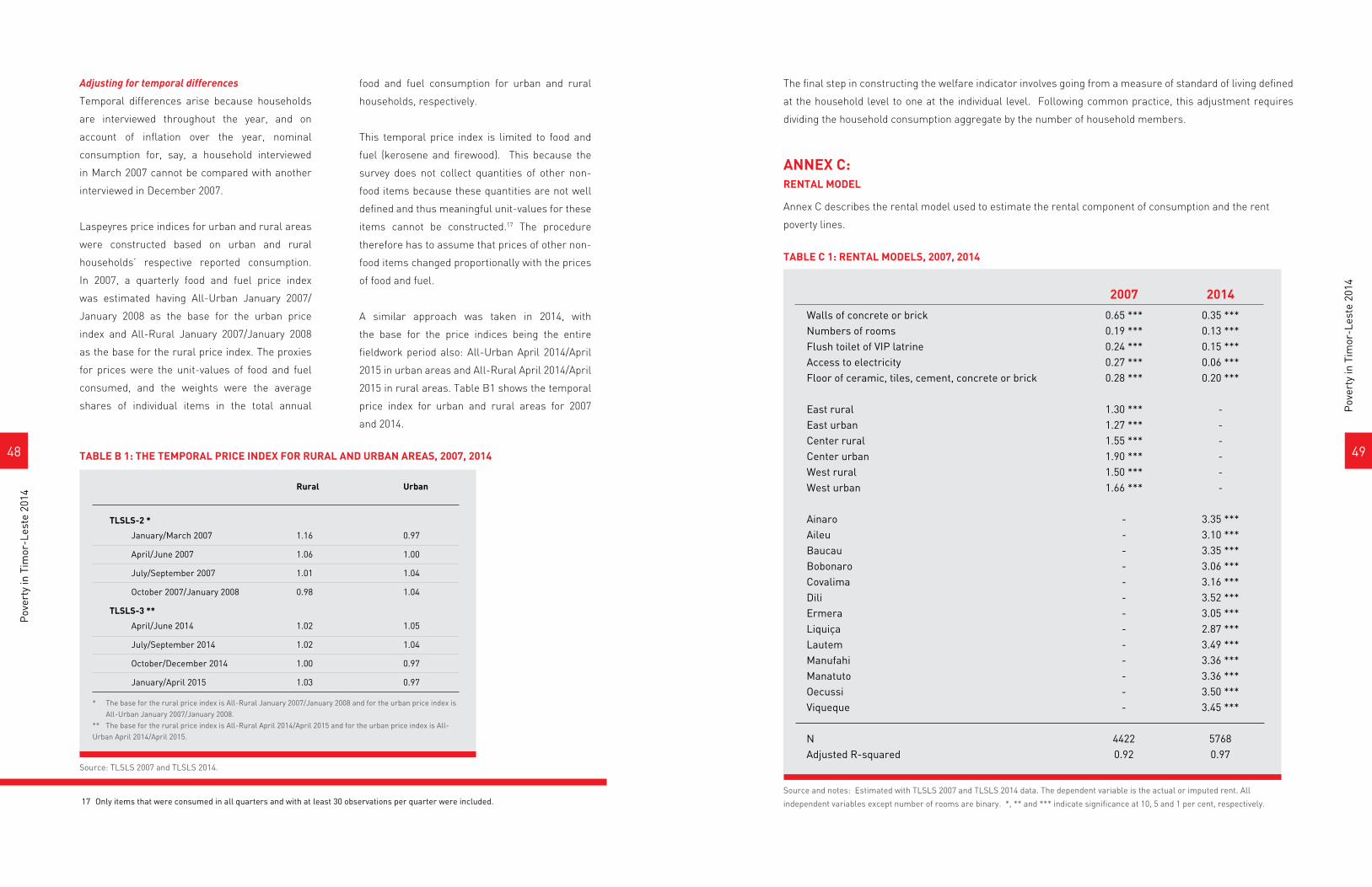
4948

Pov

erty

in T

imor

-Les

te 2

014

Pov

erty

in T

imor

-Les

te 2

014

17 Only items that were consumed in all quarters and with at least 30 observations per quarter were included.

TABLE C 1: RENTAL MODELS, 2007, 2014

Source and notes: Estimated with TLSLS 2007 and TLSLS 2014 data. The dependent variable is the actual or imputed rent. All

independent variables except number of rooms are binary. *, ** and *** indicate significance at 10, 5 and 1 per cent, respectively.

Adjusting for temporal differences

Temporal differences arise because households

are interviewed throughout the year, and on

account of inflation over the year, nominal

consumption for, say, a household interviewed

in March 2007 cannot be compared with another

interviewed in December 2007.

Laspeyres price indices for urban and rural areas

were constructed based on urban and rural

households’ respective reported consumption.

In 2007, a quarterly food and fuel price index

was estimated having All-Urban January 2007/

January 2008 as the base for the urban price

index and All-Rural January 2007/January 2008

as the base for the rural price index. The proxies

for prices were the unit-values of food and fuel

consumed, and the weights were the average

shares of individual items in the total annual

food and fuel consumption for urban and rural

households, respectively.

This temporal price index is limited to food and

fuel (kerosene and firewood). This because the

survey does not collect quantities of other non-

food items because these quantities are not well

defined and thus meaningful unit-values for these

items cannot be constructed.17 The procedure

therefore has to assume that prices of other non-

food items changed proportionally with the prices

of food and fuel.

A similar approach was taken in 2014, with

the base for the price indices being the entire

fieldwork period also: All-Urban April 2014/April

2015 in urban areas and All-Rural April 2014/April

2015 in rural areas. Table B1 shows the temporal

price index for urban and rural areas for 2007

and 2014.

2007 2014

Walls of concrete or brick 0.65 *** 0.35 ***Numbers of rooms 0.19 *** 0.13 ***Flush toilet of VIP latrine 0.24 *** 0.15 ***Access to electricity 0.27 *** 0.06 ***Floor of ceramic, tiles, cement, concrete or brick 0.28 *** 0.20 ***

East rural 1.30 *** -East urban 1.27 *** -Center rural 1.55 *** -Center urban 1.90 *** -West rural 1.50 *** -West urban 1.66 *** -

Ainaro - 3.35 ***Aileu - 3.10 ***Baucau - 3.35 ***Bobonaro - 3.06 ***Covalima - 3.16 ***Dili - 3.52 ***Ermera - 3.05 ***Liquiça - 2.87 ***Lautem - 3.49 ***Manufahi - 3.36 ***Manatuto - 3.36 ***Oecussi - 3.50 ***Viqueque - 3.45 ***

N 4422 5768Adjusted R-squared 0.92 0.97

The final step in constructing the welfare indicator involves going from a measure of standard of living defined

at the household level to one at the individual level. Following common practice, this adjustment requires

dividing the household consumption aggregate by the number of household members.

ANNEX C:RENTAL MODEL

Annex C describes the rental model used to estimate the rental component of consumption and the rent

poverty lines.

TABLE B 1: THE TEMPORAL PRICE INDEX FOR RURAL AND URBAN AREAS, 2007, 2014

Source: TLSLS 2007 and TLSLS 2014.

* The base for the rural price index is All-Rural January 2007/January 2008 and for the urban price index is All-Urban January 2007/January 2008.** The base for the rural price index is All-Rural April 2014/April 2015 and for the urban price index is All- Urban April 2014/April 2015.

Rural Urban

TLSLS-2 *

January/March 2007 1.16 0.97

April/June 2007 1.06 1.00

July/September 2007 1.01 1.04

October 2007/January 2008 0.98 1.04

TLSLS-3 **

April/June 2014 1.02 1.05

July/September 2014 1.02 1.04

October/December 2014 1.00 0.97

January/April 2015 1.03 0.97

5150

Pov

erty

in T

imor

-Les

te 2

014

Pov

erty

in T

imor

-Les

te 2

014

ANNEX D:STANDARD ERRORS AND CONFIDENCE INTERVALS

Annex D demonstrates the standard errors and confidence intervals of the 2014 poverty estimates for the

poverty incidence, poverty gap and the squared poverty gap measures.

TABLE D 2: POVERTY GAP, 2014

Poverty Standard (95% confidence interval)

incidence error Lower bound Upper bound

Timor-Leste 41.8 1.4 39.0 44.5

Rural 47.1 1.8 43.6 50.5

Urban 28.3 2.0 24.3 32.2

East 33.8 2.4 29.1 38.4

Centre 40.0 2.0 36.1 43.9

West 55.5 2.9 49.9 61.2

East Rural 36.0 2.8 30.6 41.5

East urban 21.0 3.6 13.9 28.1

Centre rural 48.3 2.7 43.0 53.7

Centre urban 26.4 2.4 21.6 31.3

West rural 57.6 3.4 51.0 64.2

West urban 46.0 4.3 37.5 54.5

Aileu 35.1 5.1 25.2 45.1

Ainaro 43.2 5.2 33.1 53.4

Baucau 32.6 3.7 25.3 39.8

Bobonaro 51.7 5.2 41.5 61.9

Cova Lima 53.1 5.7 41.8 64.3

Dili 29.1 2.5 24.2 34.0

Ermera 56.7 5.8 45.4 68.1

Lautem 31.2 4.9 22.6 41.8

Liquiça 43.0 8.1 27.1 59.0

Manufahi 47.7 5.4 37.0 58.4

Manatuto 43.1 6.1 31.1 55.0

Oecussi 62.5 3.5 55.6 69.3

Viqueque 36.9 3.7 29.6 44.2

Note: The estimation of standard errors and confidence intervals takes into account the three key features of survey design: strata,

primary sampling units and sampling weights.

Source: TLSLS 2014.

Note: The estimation of standard errors and confidence intervals takes into account the three key features of survey design: strata,

primary sampling units and sampling weights.

Source: TLSLS 2014.

Poverty Standard (95% confidence interval)

gap error Lower bound Upper bound

Timor-Leste 10.4 0.5 9.4 11.4

Rural 12.2 0.7 10.8 13.5

Urban 5.9 0.6 4.8 7.1

East 7.1 0.7 5.7 8.5

Centre 9.8 0.7 8.3 11.3

West 15.8 1.3 13.3 18.3

East Rural 7.7 0.8 6.0 9.3

East urban 3.8 0.8 2.2 5.4

Centre rural 12.6 1.1 10.4 14.7

Centre urban 5.3 0.7 3.9 6.7

West rural 16.8 1.5 13.8 19.7

West urban 11.5 1.5 8.6 14.4

Aileu 8.1 2.1 3.9 12.3

Ainaro 9.4 1.6 6.2 12.5

Baucau 6.8 1.0 4.9 8.7

Bobonaro 12.6 1.8 9.1 16.2

Cova Lima 15.9 3.1 9.8 22.0

Dili 6.0 0.7 4.6 7.5

Ermera 17.1 2.7 11.8 22.4

Lautem 6.8 1.6 3.8 9.9

Liquiça 11.7 2.4 7.0 16.5

Manufahi 11.1 1.6 8.0 14.2

Manatuto 9.2 2.3 4.8 13.7

Oecussi 19.8 0.1.7 16.5 23.1

Viqueque 7.8 1.3 5.2 10.4

TABLE D 1: POVERTY INCIDENCE, 2014

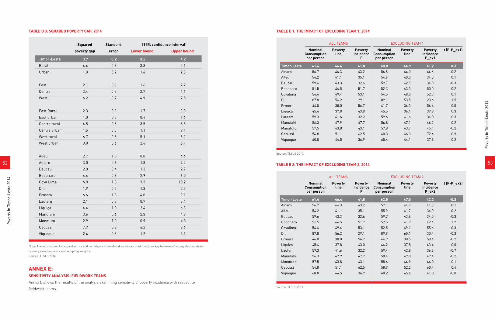
5352

Pov

erty

in T

imor

-Les

te 2

014

Pov

erty

in T

imor

-Les

te 2

014

ANNEX E:SENSITIVITY ANALYSIS: FIELDWORK TEAMS

Annex E shows the results of the analysis examining sensitivity of poverty incidence with respect to

fieldwork teams.

TABLE E 2: THE IMPACT OF EXCLUDING TEAM 2, 2014

TABLE D 3: SQUARED POVERTY GAP, 2014

ALL TEAMS EXCLUDING TEAM 2

Nominal Poverty Poverty Nominal Poverty Poverty t (P-P_ex2) Consumption line Incidence Consumption line Incidence per person P per person P_ex2

Timor-Leste 61.4 46.4 41.8 62.5 47.5 42.2 -0.2

Ainaro 56.7 44.3 43.2 57.1 44.9 44.3 0.1

Aileu 54.2 41.1 35.1 55.9 41.7 34.0 0.2

Baucau 59.6 43.3 32.6 59.7 43.6 34.0 -0.3

Bobonaro 51.5 44.5 51.7 52.5 41.9 42.4 1.2

Covalima 54.4 49.4 53.1 52.5 49.1 55.6 -0.3

Dili 87.8 56.2 29.1 89.9 60.1 30.4 -0.3

Ermera 44.0 38.0 56.7 44.9 38.5 58.4 -0.2

Liquiça 45.4 37.8 43.0 44.2 37.8 43.4 0.0

Lautem 59.3 41.6 32.2 59.4 42.8 36.6 -0.7

Manufahi 56.3 47.9 47.7 58.4 49.8 49.4 -0.2

Manatuto 57.5 43.8 43.1 58.6 44.9 44.0 -0.1

Oecussi 54.8 51.1 62.5 58.9 52.2 60.4 0.4

Viqueque 60.0 44.5 36.9 60.2 45.6 41.0 -0.8

TABLE E 1: THE IMPACT OF EXCLUDING TEAM 1, 2014

ALL TEAMS EXCLUDING TEAM 1

Nominal Poverty Poverty Nominal Poverty Poverty t (P-P_ex1) Consumption line Incidence Consumption line Incidence per person P per person P_ex1

Timor-Leste 61.4 46.4 41.8 60.8 44.9 41.2 0.3

Ainaro 56.7 44.3 43.2 56.8 44.0 44.6 -0.2

Aileu 54.2 41.1 35.1 54.6 40.0 34.0 0.1

Baucau 59.6 43.3 32.6 59.7 42.9 34.0 -0.3

Bobonaro 51.5 44.5 51.7 52.3 43.3 50.0 0.2

Covalima 54.4 49.4 53.1 54.5 48.0 52.3 0.1

Dili 87.8 56.2 29.1 89.1 53.5 23.6 1.5

Ermera 44.0 38.0 56.7 41.7 36.3 56.4 0.0

Liquiça 45.4 37.8 43.0 45.5 36.1 39.8 0.3

Lautem 59.3 41.6 32.2 59.6 41.4 34.0 -0.3

Manufahi 56.3 47.9 47.7 56.8 47.1 46.2 0.2

Manatuto 57.5 43.8 43.1 57.8 43.7 45.1 -0.2

Oecussi 54.8 51.1 62.5 40.3 46.3 72.4 -0.9

Viqueque 60.0 44.5 36.9 60.4 44.1 37.8 -0.2

Note: The estimation of standard errors and confidence intervals takes into account the three key features of survey design: strata,

primary sampling units and sampling weights.

Source: TLSLS 2014.

Squared Standard (95% confidence interval)

poverty gap error Lower bound Upper bound

Timor-Leste 3.7 0.2 3.2 4.2

Rural 4.4 0.3 3.8 5.1

Urban 1.8 0.2 1.4 2.3

East 2.1 0.3 1.6 2.7

Centre 3.4 0.3 2.7 4.1

West 6.2 0.7 4.9 7.5

East Rural 2.3 0.3 1.7 3.0

East urban 1.0 0.3 0.4 1.6

Centre rural 4.5 0.5 3.5 5.5

Centre urban 1.6 0.3 1.1 2.1

West rural 6.7 0.8 5.1 8.2

West urban 3.8 0.6 2.6 5.1

Aileu 2.7 1.0 0.8 4.6

Ainaro 3.0 0.6 1.8 4.2

Baucau 2.0 0.4 1.3 2.7

Bobonaro 4.4 0.8 2.9 6.0

Cova Lima 6.8 1.8 3.3 10.2

Dili 1.9 0.3 1.3 2.5

Ermera 6.6 1.3 4.0 9.1

Lautem 2.1 0.7 0.7 3.4

Liquiça 4.4 1.0 2.4 6.3

Manufahi 3.6 0.6 2.3 4.8

Manatuto 2.9 1.0 0.9 4.8

Oecussi 7.9 0.9 6.2 9.6

Viqueque 2.4 0.6 1.2 3.5

Source: TLSLS 2014.

Source: TLSLS 2014.

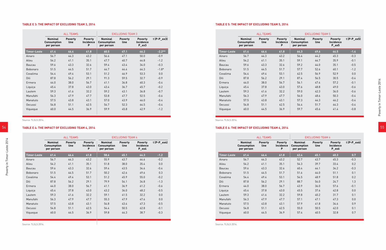
5554

Pov

erty

in T

imor

-Les

te 2

014

Pov

erty

in T

imor

-Les

te 2

014

Source: TLSLS 2014.Source: TLSLS 2014.

TABLE E 5: THE IMPACT OF EXCLUDING TEAM 5, 2014 TABLE E 3: THE IMPACT OF EXCLUDING TEAM 3, 2014

ALL TEAMS EXCLUDING TEAM 5

Nominal Poverty Poverty Nominal Poverty Poverty t (P-P_ex5) Consumption line Incidence Consumption line Incidence per person P per person P_ex5

Timor-Leste 61.4 46.4 41.8 64.3 49.6 44.5 -1.4

Ainaro 56.7 44.3 43.2 56.4 44.2 45.3 -0.3

Aileu 54.2 41.1 35.1 59.1 44.7 35.9 -0.1

Baucau 59.6 43.3 32.6 59.2 44.0 35.1 -0.5

Bobonaro 51.5 44.5 51.7 57.7 52.6 60.1 -1.2

Covalima 54.4 49.4 53.1 62.5 56.9 52.9 0.0

Dili 87.8 56.2 29.1 87.4 56.5 30.5 -0.4

Ermera 44.0 38.0 56.7 56.1 47.4 57.2 -0.1

Liquiça 45.4 37.8 43.0 57.6 48.8 49.0 -0.6

Lautem 59.3 41.6 32.2 59.0 42.3 36.0 -0.6

Manufahi 56.3 47.9 47.7 56.0 48.6 50.3 -0.4

Manatuto 57.5 43.8 43.1 57.3 44.3 46.2 -0.4

Oecussi 54.8 51.1 62.5 54.4 51.7 64.3 -0.4

Viqueque 60.0 44.5 36.9 59.7 45.6 41.4 -0.8

ALL TEAMS EXCLUDING TEAM 3

Nominal Poverty Poverty Nominal Poverty Poverty t (P-P_ex3) Consumption line Incidence Consumption line Incidence per person P per person P_ex3

Timor-Leste 61.4 46.4 41.8 60.5 47.1 46.2 -2.2**

Ainaro 56.7 44.3 43.2 56.6 47.1 50.0 -0.9

Aileu 54.2 41.1 35.1 47.7 40.7 44.8 -1.2

Baucau 59.6 43.3 32.6 59.4 43.4 34.0 -0.3

Bobonaro 51.5 44.5 51.7 44.7 44.4 64.3 -1.8*

Covalima 54.4 49.4 53.1 51.2 46.9 53.3 0.0

Dili 87.8 56.2 29.1 91.3 59.5 32.7 -0.9

Ermera 44.0 38.0 56.7 41.1 36.8 60.3 -0.4

Liquiça 45.4 37.8 43.0 43.4 36.7 45.7 -0.2

Lautem 59.3 41.6 32.2 59.2 43.1 36.8 -0.7

Manufahi 56.3 47.9 47.7 53.8 47.7 52.5 -0.6

Manatuto 57.5 43.8 43.1 57.0 43.9 46.0 -0.4

Oecussi 54.8 51.1 62.5 54.7 52.3 64.5 -0.4

Viqueque 60.0 44.5 36.9 59.9 45.8 42.9 -1.2

TABLE E 6: THE IMPACT OF EXCLUDING TEAM 6, 2014

ALL TEAMS EXCLUDING TEAM 6

Nominal Poverty Poverty Nominal Poverty Poverty t (P-P_ex6) Consumption line Incidence Consumption line Incidence per person P per person P_ex6

Timor-Leste 61.4 46.4 41.8 62.4 45.1 40.3 0.7

Ainaro 56.7 44.3 43.2 52.7 43.7 45.3 -0.3

Aileu 54.2 41.1 35.1 54.3 39.7 33.4 0.2

Baucau 59.6 43.3 32.6 60.4 44.1 34.2 -0.3

Bobonaro 51.5 44.5 51.7 51.6 44.0 51.1 0.1

Covalima 54.4 49.4 53.1 54.5 48.9 51.8 0.2

Dili 87.8 56.2 29.1 88.7 54.0 24.7 1.3

Ermera 44.0 38.0 56.7 43.9 36.0 57.6 -0.1

Liquiça 45.4 37.8 43.0 45.5 37.6 42.8 0.0

Lautem 59.3 41.6 32.2 59.8 40.2 31.7 0.1

Manufahi 56.3 47.9 47.7 57.1 47.1 47.3 0.0

Manatuto 57.5 43.8 43.1 57.9 41.8 34.6 0.9

Oecussi 54.8 51.1 62.5 55.0 50.5 62.0 0.1

Viqueque 60.0 44.5 36.9 57.4 40.5 32.8 0.7

TABLE E 4: THE IMPACT OF EXCLUDING TEAM 4, 2014

ALL TEAMS EXCLUDING TEAM 4

Nominal Poverty Poverty Nominal Poverty Poverty t (P-P_ex4) Consumption line Incidence Consumption line Incidence per person P per person P_ex4

Timor-Leste 61.4 46.4 41.8 58.6 45.1 44.3 -1.2

Ainaro 56.7 44.3 43.2 55.9 43.7 44.6 -0.2

Aileu 54.2 41.1 35.1 51.8 38.0 35.4 0.0

Baucau 59.6 43.3 32.6 59.4 43.5 34.6 -0.4

Bobonaro 51.5 44.5 51.7 50.2 42.6 49.6 0.3

Covalima 54.4 49.4 53.1 51.2 45.9 55.0 -0.2

Dili 87.8 56.2 29.1 79.9 54.1 34.8 -1.3

Ermera 44.0 38.0 56.7 41.1 36.9 61.2 -0.6

Liquiça 45.4 37.8 43.0 43.2 36.0 48.2 -0.5

Lautem 59.3 41.6 32.2 59.1 41.5 32.2 0.0

Manufahi 56.3 47.9 47.7 55.3 47.9 47.6 0.0

Manatuto 57.5 43.8 43.1 54.8 43.4 47.3 -0.5

Oecussi 54.8 51.1 62.5 54.4 50.5 62.8 -0.1

Viqueque 60.0 44.5 36.9 59.8 44.3 38.7 -0.3

Source: TLSLS 2014.Source: TLSLS 2014.

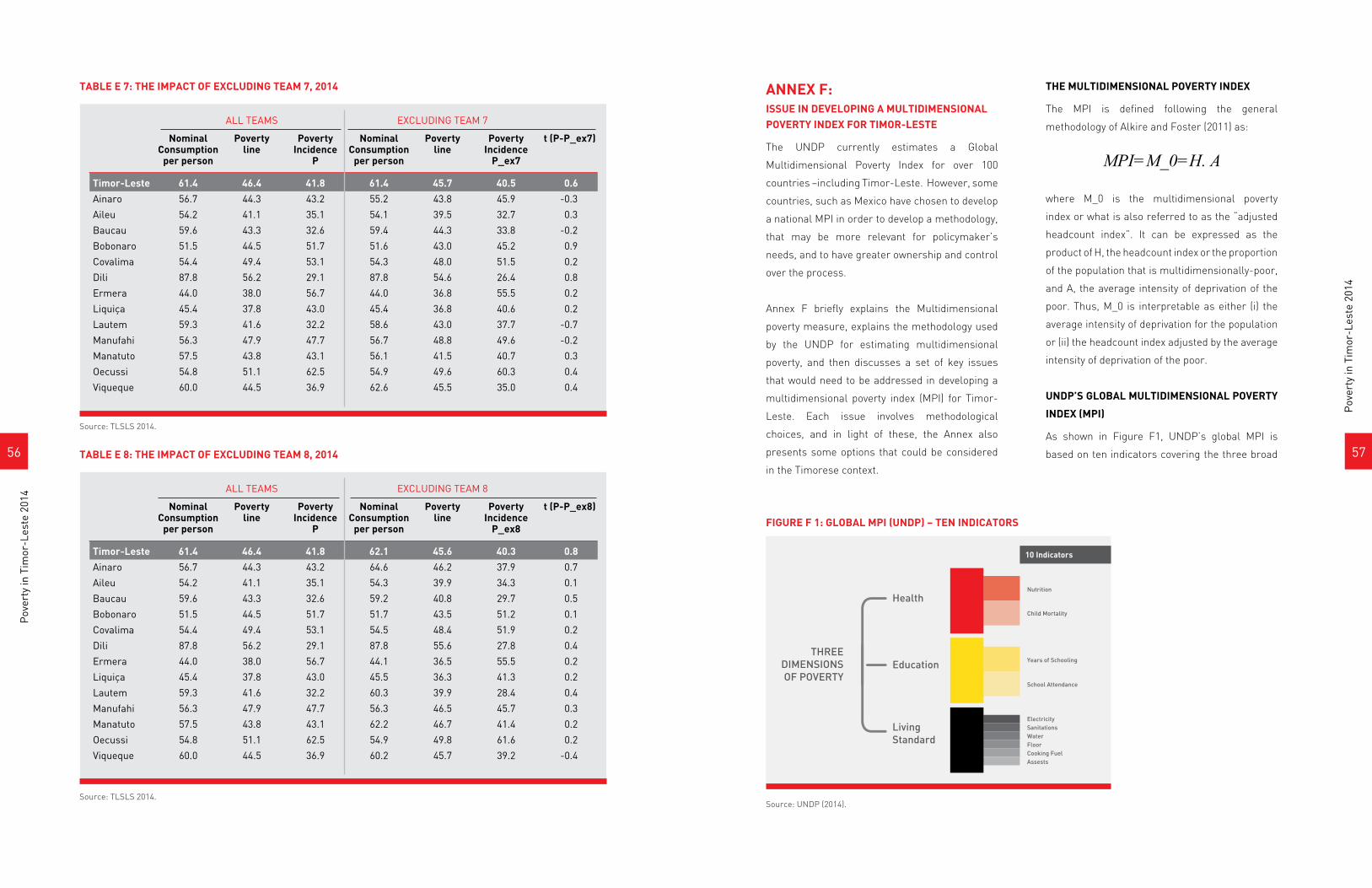
5756

Pov

erty

in T

imor

-Les

te 2

014

Pov

erty

in T

imor

-Les

te 2

014

ANNEX F:ISSUE IN DEVELOPING A MULTIDIMENSIONAL POVERTY INDEX FOR TIMOR-LESTE

The UNDP currently estimates a Global

Multidimensional Poverty Index for over 100

countries –including Timor-Leste. However, some

countries, such as Mexico have chosen to develop

a national MPI in order to develop a methodology,

that may be more relevant for policymaker’s

needs, and to have greater ownership and control

over the process.

Annex F briefly explains the Multidimensional

poverty measure, explains the methodology used

by the UNDP for estimating multidimensional

poverty, and then discusses a set of key issues

that would need to be addressed in developing a

multidimensional poverty index (MPI) for Timor-

Leste. Each issue involves methodological

choices, and in light of these, the Annex also

presents some options that could be considered

in the Timorese context.

THE MULTIDIMENSIONAL POVERTY INDEX

The MPI is defined following the general

methodology of Alkire and Foster (2011) as:

MPI=M_0=H. A

where M_0 is the multidimensional poverty

index or what is also referred to as the “adjusted

headcount index”. It can be expressed as the

product of H, the headcount index or the proportion

of the population that is multidimensionally-poor,

and A, the average intensity of deprivation of the

poor. Thus, M_0 is interpretable as either (i) the

average intensity of deprivation for the population

or (ii) the headcount index adjusted by the average

intensity of deprivation of the poor.

UNDP’S GLOBAL MULTIDIMENSIONAL POVERTY

INDEX (MPI)

As shown in Figure F1, UNDP’s global MPI is

based on ten indicators covering the three broad

THREEDIMENSIONSOF POVERTY

HealthNutrition

Child Mortality

Years of Schooling

School Attendance

ElectricitySanitationsWaterFloorCooking FuelAssests

10 Indicators

Education

LivingStandard

FIGURE F 1: GLOBAL MPI (UNDP) – TEN INDICATORS

Source: UNDP (2014).

TABLE E 7: THE IMPACT OF EXCLUDING TEAM 7, 2014

ALL TEAMS EXCLUDING TEAM 7

Nominal Poverty Poverty Nominal Poverty Poverty t (P-P_ex7) Consumption line Incidence Consumption line Incidence per person P per person P_ex7

Timor-Leste 61.4 46.4 41.8 61.4 45.7 40.5 0.6

Ainaro 56.7 44.3 43.2 55.2 43.8 45.9 -0.3

Aileu 54.2 41.1 35.1 54.1 39.5 32.7 0.3

Baucau 59.6 43.3 32.6 59.4 44.3 33.8 -0.2

Bobonaro 51.5 44.5 51.7 51.6 43.0 45.2 0.9

Covalima 54.4 49.4 53.1 54.3 48.0 51.5 0.2

Dili 87.8 56.2 29.1 87.8 54.6 26.4 0.8

Ermera 44.0 38.0 56.7 44.0 36.8 55.5 0.2

Liquiça 45.4 37.8 43.0 45.4 36.8 40.6 0.2

Lautem 59.3 41.6 32.2 58.6 43.0 37.7 -0.7

Manufahi 56.3 47.9 47.7 56.7 48.8 49.6 -0.2

Manatuto 57.5 43.8 43.1 56.1 41.5 40.7 0.3

Oecussi 54.8 51.1 62.5 54.9 49.6 60.3 0.4

Viqueque 60.0 44.5 36.9 62.6 45.5 35.0 0.4

TABLE E 8: THE IMPACT OF EXCLUDING TEAM 8, 2014

ALL TEAMS EXCLUDING TEAM 8

Nominal Poverty Poverty Nominal Poverty Poverty t (P-P_ex8) Consumption line Incidence Consumption line Incidence per person P per person P_ex8

Timor-Leste 61.4 46.4 41.8 62.1 45.6 40.3 0.8

Ainaro 56.7 44.3 43.2 64.6 46.2 37.9 0.7

Aileu 54.2 41.1 35.1 54.3 39.9 34.3 0.1

Baucau 59.6 43.3 32.6 59.2 40.8 29.7 0.5

Bobonaro 51.5 44.5 51.7 51.7 43.5 51.2 0.1

Covalima 54.4 49.4 53.1 54.5 48.4 51.9 0.2

Dili 87.8 56.2 29.1 87.8 55.6 27.8 0.4

Ermera 44.0 38.0 56.7 44.1 36.5 55.5 0.2

Liquiça 45.4 37.8 43.0 45.5 36.3 41.3 0.2

Lautem 59.3 41.6 32.2 60.3 39.9 28.4 0.4

Manufahi 56.3 47.9 47.7 56.3 46.5 45.7 0.3

Manatuto 57.5 43.8 43.1 62.2 46.7 41.4 0.2

Oecussi 54.8 51.1 62.5 54.9 49.8 61.6 0.2

Viqueque 60.0 44.5 36.9 60.2 45.7 39.2 -0.4

Source: TLSLS 2014.

Source: TLSLS 2014.

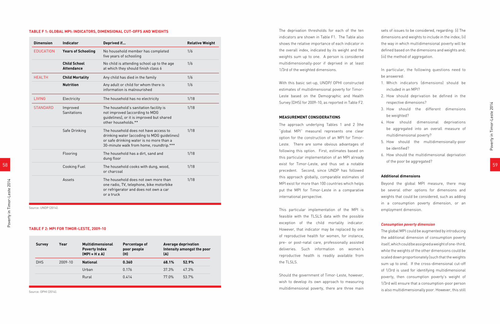
5958

Pov

erty

in T

imor

-Les

te 2

014

Pov

erty

in T

imor

-Les

te 2

014

The deprivation thresholds for each of the ten

indicators are shown in Table F1. The Table also

shows the relative importance of each indicator in

the overall index, indicated by its weight and the

weights sum up to one. A person is considered

multidimensionally-poor if deprived in at least

1/3rd of the weighted dimensions.

With this basic set-up, UNDP/ OPHI constructed

estimates of multidimensional poverty for Timor-

Leste based on the Demographic and Health

Survey (DHS) for 2009-10, as reported in Table F2.

MEASUREMENT CONSIDERATIONS

The approach underlying Tables 1 and 2 (the

“global MPI” measure) represents one clear

option for the construction of an MPI for Timor-

Leste. There are some obvious advantages of

following this option. First, estimates based on

this particular implementation of an MPI already

exist for Timor-Leste, and thus set a notable

precedent. Second, since UNDP has followed

this approach globally, comparable estimates of

MPI exist for more than 100 countries which helps

put the MPI for Timor-Leste in a comparative

international perspective.

This particular implementation of the MPI is

feasible with the TLSLS data with the possible

exception of the child mortality indicator.

However, that indicator may be replaced by one

of reproductive health for women, for instance,

pre- or post-natal care, professionally assisted

deliveries. Such information on women’s

reproductive health is readily available from

the TLSLS.

Should the government of Timor-Leste, however,

wish to develop its own approach to measuring

multidimensional poverty, there are three main

sets of issues to be considered, regarding: (i) The

dimensions and weights to include in the index; (ii)

the way in which multidimensional poverty will be

defined based on the dimensions and weights and;

(iii) the method of aggregation.

In particular, the following questions need to

be answered:

1. Which indicators (dimensions) should be

included in an MPI?

2. How should deprivation be defined in the

respective dimensions?

3. How should the different dimensions

be weighted?

4. How should dimensional deprivations

be aggregated into an overall measure of

multidimensional poverty?

5. How should the multidimensionally-poor

be identified?

6. How should the multidimensional deprivation

of the poor be aggregated?

Additional dimensions

Beyond the global MPI measure, there may

be several other options for dimensions and

weights that could be considered, such as adding

in a consumption poverty dimension, or an

employment dimension.

Consumption poverty dimension

The global MPI could be augmented by introducing

the additional dimension of consumption poverty

itself, which could be assigned a weight of one-third,

while the weights of the other dimensions could be

scaled down proportionately (such that the weights

sum up to one). If the cross-dimensional cut-off

of 1/3rd is used for identifying multidimensional

poverty, then consumption poverty’s weight of

1/3rd will ensure that a consumption-poor person

is also multidimensionally poor. However, this still

TABLE F 2: MPI FOR TIMOR-LESTE, 2009-10

TABLE F 1: GLOBAL MPI: INDICATORS, DIMENSIONAL CUT-OFFS AND WEIGHTS

Source: UNDP (2014).

Source: OPHI (2014).

Dimension Indicator Deprived if... Relative Weight

EDUCATION Years of Schooling No household member has completed 1/6 five years of schooling

Child School No child is attending school up to the age 1/6 Attendance at which they should finish class 6

HEALTH Child Mortality Any child has died in the family 1/6

Nutrition Any adult or child for whom there is 1/6 information is malnourished

LIVING Electricity The household has no electricity 1/18

STANDARD Improved The household’s sanitation facility is 1/18 Sanitations not improved (according to MDG guidelines), or it is improved but shared other households.**

Safe Drinking The household does not have access to 1/18 drinking water (accoding to MDG guidelines) or safe drinking water is no more than a 30-minute walk from home, roundtrip.***

Flooring The household has a dirt, sand and 1/18 dung floor

Cooking Fuel The household cooks with dung, wood, 1/18 or charcoal

Assets The household does not own more than 1/18 one radio, TV, telephone, bike motorbike or refrigerator and does not own a car or a truck

Survey Year Multidimensional Percentage of Average deprivation Poverty Index poor people Intensity amongst the poor (MPI = H x A) (H) (A)

DHS 2009-10 National 0.360 68.1% 52.9%

Urban 0.176 37.3% 47.3%

Rural 0.414 77.0% 53.7%

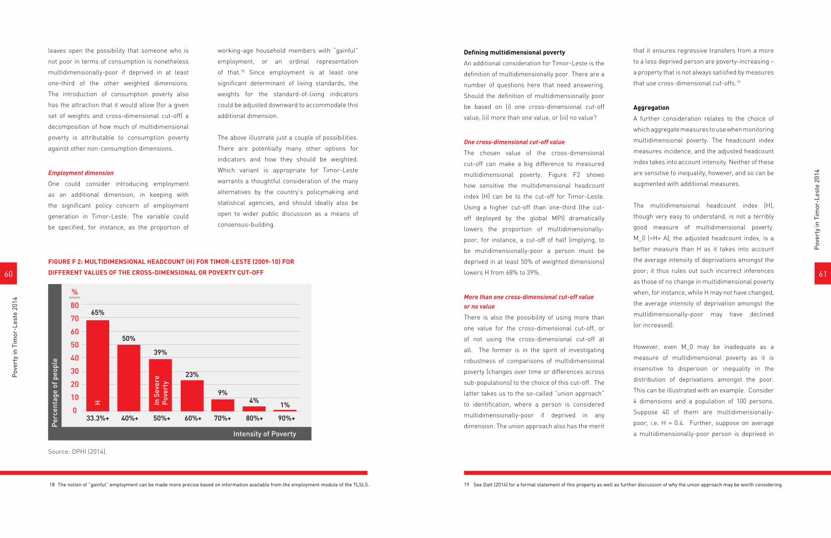
6160

Pov

erty

in T

imor

-Les

te 2

014

Pov

erty

in T

imor

-Les

te 2

014

Defining multidimensional poverty

An additional consideration for Timor-Leste is the

definition of multidimensionally poor. There are a

number of questions here that need answering.

Should the definition of multidimensionally poor

be based on (i) one cross-dimensional cut-off

value, (ii) more than one value, or (iii) no value?

One cross-dimensional cut-off value

The chosen value of the cross-dimensional

cut-off can make a big difference to measured

multidimensional poverty. Figure F2 shows

how sensitive the multidimensional headcount

index (H) can be to the cut-off for Timor-Leste.

Using a higher cut-off than one-third (the cut-

off deployed by the global MPI) dramatically

lowers the proportion of multidimensionally-

poor; for instance, a cut-off of half (implying, to

be mutidimensionally-poor a person must be

deprived in at least 50% of weighted dimensions)

lowers H from 68% to 39%.

More than one cross-dimensional cut-off valueor no value

There is also the possibility of using more than

one value for the cross-dimensional cut-off, or

of not using the cross-dimensional cut-off at

all. The former is in the spirit of investigating

robustness of comparisons of multidimensional

poverty (changes over time or differences across

sub-populations) to the choice of this cut-off. The

latter takes us to the so-called “union approach”

to identification, where a person is considered

multidimensionally-poor if deprived in any

dimension. The union approach also has the merit

that it ensures regressive transfers from a more

to a less deprived person are poverty-increasing –

a property that is not always satisfied by measures

that use cross-dimensional cut-offs.19

Aggregation

A further consideration relates to the choice of

which aggregate measures to use when monitoring

multidimensional poverty. The headcount index

measures incidence, and the adjusted headcount

index takes into account intensity. Neither of these

are sensitive to inequality, however, and so can be

augmented with additional measures.

The multidimensional headcount index (H),

though very easy to understand, is not a terribly

good measure of multidimensional poverty.

M_0 (=H× A), the adjusted headcount index, is a

better measure than H as it takes into account

the average intensity of deprivations amongst the

poor; it thus rules out such incorrect inferences

as those of no change in multidimensional poverty

when, for instance, while H may not have changed,

the average intensity of deprivation amongst the

multidimensionally-poor may have declined

(or increased).

However, even M_0 may be inadequate as a

measure of multidimensional poverty as it is

insensitive to dispersion or inequality in the

distribution of deprivations amongst the poor.

This can be illustrated with an example. Consider

4 dimensions and a population of 100 persons.

Suppose 40 of them are multidimensionally-

poor, i.e. H = 0.4. Further, suppose on average

a multidimensionally-poor person is deprived in

Source: OPHI (2014).

18 The notion of “gainful” employment can be made more precise based on information available from the employment module of the TLSLS. 19 See Datt (2014) for a formal statement of this property as well as further discussion of why the union approach may be worth considering.

FIGURE F 2: MULTIDIMENSIONAL HEADCOUNT (H) FOR TIMOR-LESTE (2009-10) FOR

DIFFERENT VALUES OF THE CROSS-DIMENSIONAL OR POVERTY CUT-OFF

leaves open the possibility that someone who is

not poor in terms of consumption is nonetheless

multidimensionally-poor if deprived in at least

one-third of the other weighted dimensions.

The introduction of consumption poverty also

has the attraction that it would allow (for a given

set of weights and cross-dimensional cut-off) a

decomposition of how much of multidimensional

poverty is attributable to consumption poverty

against other non-consumption dimensions.

Employment dimension

One could consider introducing employment

as an additional dimension, in keeping with

the significant policy concern of employment

generation in Timor-Leste. The variable could

be specified, for instance, as the proportion of

working-age household members with “gainful”

employment, or an ordinal representation

of that.18 Since employment is at least one

significant determinant of living standards, the

weights for the standard-of-living indicators

could be adjusted downward to accommodate this

additional dimension.

The above illustrate just a couple of possibilities.

There are potentially many other options for

indicators and how they should be weighted.

Which variant is appropriate for Timor-Leste

warrants a thoughtful consideration of the many

alternatives by the country’s policymaking and

statistical agencies, and should ideally also be

open to wider public discussion as a means of

consensus-building.

Intensity of Poverty

60

70

80

%

50

40

30

20

10

0

Per

cent

age

of p

eopl

e

33.3%+

65%

50%

39%

23%

9%4%

1%H In S

ever

eP

over

ty

40%+ 50%+ 60%+ 70%+ 80%+ 90%+

6362

Pov

erty

in T

imor

-Les

te 2

014

Pov

erty

in T

imor

-Les

te 2

014

Alkire, S., Foster, J.E. (2011): Counting and multidimensional poverty measurement. Journal of Public Economics,

95(7-8): 476-487.

Datt, Gaurav (2014): Making every deprivation count: multidimensional poverty without the “dual cut-off”. Working

Paper, Monash University.

Deaton, Angus (1997): The Analysis of Household Surveys. World Bank and Johns Hopkins University Press,

Baltimore.

Foster, J. (2005): Poverty indices. In: A. de Janvry and R. Kanbur (eds.) Poverty, Inequality and Development: Essays

in Honor of Erik Thorbecke, Kluwer Academic Publishers.

Foster, J., Greer, J. and E. Thorbecke (1984). A Class of Decomposable Poverty Measures, Econometrica, 52:

761-765.

OPHI (2014). “Timor-Leste Country Briefing”, Multidimensional Poverty Index Data Bank. Oxford Poverty and

Human Development Initiative (OPHI), University of Oxford. Available at: www.ophi.org.uk/multidimensional-

poverty-index/mpi-country-briefings

National Institute of Nutrition and Indian Council of Medical Research (NIN-ICMR) (2011): Dietary Guidelines

for Indians – A Manual, Second Edition, Hyderabad.

Ravallion, Martin. (2008). “Poverty Lines” in The New Palgrave Dictionary of Economics. 2nd Edition, Larry

Blume and Steven Derlauf (eds), Palgrave Macmillan, London.

_____ (2016): Economics of Poverty: History, Measurement and Policy. Oxford University Press.

Sen, Amartya (1976). Poverty: An Ordinal Approach to Measurement, Econometrica, 46: 437-446.

REFERENCES

50% of dimensions (or two dimensions), i.e. A =

0.5. Then, the MPI measure M_0 = 0.4 x 0.5 = 0.2.

But note that the measure M_0 can also be written

as M_0 = (total number of deprived dimensions of

the poor / total number of possible deprivations) =

(80 / 400) = 0.2.

M_0 depends on the total number of deprivations

but not their dispersion or concentration,

which is a limitation if one wants the measure

of multidimensional poverty to be sensitive to

the degree of inequality in the distribution of

deprivations. Measures with such sensitivity do

exist and may be worth considering (Datt, 2014).

And again, one should not underrate the possibility

of using more than one aggregate measure of

multidimensional poverty.

64

Pov

erty

in T

imor

-Les

te 2

014

_____ (1980): “Equality of what?” (Lecture delivered at Stanford University, 22 May 1979), in MacMurrin, Sterling

M., The Tanner lectures on human values 1, Salt Lake City, Utah: University of Utah Press.

_____ (1985): Commodities and Capabilities. New York, NY: North-Holland.

_____ (1999): Development as Freedom. New York: Oxford University Press.

UNDP (2014): Human Development Report 2014: Sustaining Human Progress: Reducing Vulnerability and Building

Resilience. Macmillan, New York.

World Bank (2003). Timor-Leste: Poverty in a New Nation: Analysis for Action, Washington DC.

World Bank (2008). Timor-Leste: Poverty in a Young Nation. Dili and Washington DC.