University of North Dakota University of North Dakota

UND Scholarly Commons UND Scholarly Commons

Theses and Dissertations Theses, Dissertations, and Senior Projects

1-1-2019

Potentials Of Physiological Signals To Implement A Wearable Potentials Of Physiological Signals To Implement A Wearable

Drowsiness Detection And Warning System For Pilots Drowsiness Detection And Warning System For Pilots

Shubha Majumder

Follow this and additional works at: https://commons.und.edu/theses

Recommended Citation Recommended Citation Majumder, Shubha, "Potentials Of Physiological Signals To Implement A Wearable Drowsiness Detection And Warning System For Pilots" (2019). Theses and Dissertations. 2861. https://commons.und.edu/theses/2861

This Thesis is brought to you for free and open access by the Theses, Dissertations, and Senior Projects at UND Scholarly Commons. It has been accepted for inclusion in Theses and Dissertations by an authorized administrator of UND Scholarly Commons. For more information, please contact und.commons@library.und.edu.

POTENTIALS OF PHYSIOLOGICAL SIGNALS TO IMPLEMENT A WEARABLE

DROWSINESS DETECTION AND WARNING SYSTEM FOR PILOTS

by

Shubha Majumder

Bachelor of Science in Electrical and Electronic Engineering

Chittagong University of Engineering and Technology, Bangladesh

A Thesis

Submitted to the Graduate Faculty

of the

University of North Dakota

in partial fulfillment of the requirements

for the degree of

Master of Science in Biomedical Engineering

Grand Forks, North Dakota

December

2019

ii

© 2019 Shubha Majumder and Dr. Kouhyar Tavakolian

iii

iv

PERMISSION

Title Potentials of Physiological Signals to Implement a Wearable

Drowsiness Detection and Warning System for Pilots

Department Biomedical Engineering

Degree Master of Science

In presenting this thesis in partial fulfillment of the requirements for a graduate degree from

the University of North Dakota, I agree that the library of this University shall make it freely

available for inspection. I further agree that permission for extensive copying for scholarly

purposes may be granted by the professor who supervised my thesis work or, in his absence, by

the chairperson of the department or the dean of the Graduate School. It is understood that any

copying or publication or other use of this thesis or part thereof for financial gain shall not be

allowed without my written permission. It is also understood that due recognition shall be given

to me and to the University of North Dakota in any scholarly use which may be made of any

material in my thesis.

Shubha Majumder

December 04, 2019

v

TABLE OF CONTENTS

Contents Page

LIST OF FIGURES vii

LIST OF TABLES ix

ACKNOWLEDGMENTS xii

ABSTRACT xiv

ABBREVIATIONS xvi

CHAPTER 1 INTRODUCTION 17

1.1 Motivation 17

1.2 Defining Drowsiness 18

1.3 Approaches used for Onboard Drowsiness Detection 19

1.3.1 Vehicle-based measure 20

1.3.2 Behavioral measure 22

1.3.3 Physiological signal-based measure 25

1.3.4 Subjective measure 29

1.4 Simulator based Study 31

1.5 Discussion 33

CHAPTER 2 METHODOLOGY 34

2.1 Commonly used Physiological Signals 34

2.1.1 Electrocardiogram (ECG) 34

2.1.2 Electroencephalogram (EEG) 36

2.1.3 Electrooculogram (EOG) 39

2.1.4 Photoplethysmogram (PPG) 40

vi

2.1.5 Electromyogram (EMG) 41

2.2 Our System 42

2.3 Data Acquisition 43

2.4 Data Analysis 47

2.5 Discussion 49

CHAPTER 3 RESULTS 50

3.1 Heart Rate Variability (HRV) Analysis 50

3.2 Pulse Rate Variability (PRV) Analysis 61

3.3 Pulse Arrival Time (PAT) Analysis 63

3.4 PPG Waveform based Features Extraction 69

3.5 EEG Spectral Analysis 78

3.6 Machine Learning for Drowsy Periods Detection 82

CHAPTER 4 DISCUSSION 84

CHAPTER 5 CONCLUSION, FUTURE WORK, AND CONTRIBUTION 94

5.1 Conclusion 94

5.2 Limitations 95

5.3 Future work 96

5.4 My Contribution 96

BIBLIOGRAPHY 98

vii

LIST OF FIGURES

Figure Page

Figure 1. Drowsiness detection using physiological measures 26

Figure 2. Photos of the National Higher French Institute of Aeronautics and Space

(Institut Supérieur de l’Aéronautique et de l’Espace-ISAE) flight simulator. Cockpit

view (left panel) and the view from outside of the simulator (right panel) [92]

32

Figure 3. A normal Electrocardiogram tracing [96] 36

Figure 4. Four lobes of the human brain [103] 37

Figure 5. EEG electrodes placement using 10-20 electrode placement system [109] 38

Figure 6. Anatomy of a normal human eye [114] 39

Figure 7. Horizontal and vertical electrooculography (EOG) [112] 40

Figure 8. Photoplethysmography (PPG) technique (transmission and reflection type)

[115]

41

Figure 9. Desired headset system for drowsiness detection and warning 43

Figure 10. a) Simulated flight, b) placement of EEG, ECG, PPG, and EOG electrodes

[11]

45

Figure 11. RR interval variation [129] 51

Figure 12. Heart rate variability over 24 hours [121] 52

Figure 13. Pulse arrival time (PAT) calculation technique [11] 64

Figure 14. Pulse arrival time (PAT) comparison during baseline and drowsy periods

(mean± SE). (Black and red color indicate during the baseline and drowsy periods

respectively) [11]

66

Figure 15. RR interval and PAT/RR (%) comparison for each subject during baseline

and drowsy periods. (Black and red color indicate during the baseline and drowsy

periods respectively) [11]

66

Figure 16. All the PAT and RR intervals comparison (Baseline vs Drowsy) 67

Figure 17. Comparison of baseline and drowsy PAT using PPG foot and PPG first

derivative peak

68

viii

Figure 18. Comparison of baseline and drowsy PAT using PPG second derivative

peak

69

Figure 19. PPG waveform based features extraction [11] 70

Figure 20. Increase in PPG crest time and diastolic time (Mean ± standard error (SE))

during drowsy periods compared to alert periods [11]

71

Figure 21. PPG width-based features extraction (both systolic and diastolic side) 72

Figure 22. PPG waveform timing features extraction 76

Figure 23. Signal processing steps followed to compute relative spectral power

distribution in the respective EEG frequency bands [119]

79

Figure 24. Relative spectral power distribution (mean±SE) in four EEG frequency

bands: δ, θ, α, and β during three psychological states (baseline (BL), microsleeps

(MS), and longsleeps (LS)) in five brain regions ((Frontal, F), (Central, C), (Parietal,

P), (Temporal, T), and (Occipital, O)). The x-axis represents three psychological states

and the y-axis represents relative PSD [119]

81

Figure 25. Changes observed in four ratio indices (mean±SE) during three

psychological states (Baseline (BL microsleeps (MS), and longsleeps (LS)) in five

brain regions ((Frontal, F), (Central, C), (Parietal, P), (Temporal, T), and (Occipital,

O)). The x-axis represents three psychological states and the y-axis represents relative

PSD [119]

82

ix

LIST OF TABLES

Table Page

Table 1. Previous works based on vehicle-based measure 21

Table 2. Previous works based on operator’s behavioral measure 24

Table 3. Notable studies conducted using physiological signal based measure 28

Table 4. Rating and meaning of the Karolinska Sleepiness Scale (KSS) [20] 30

Table 5. Basic information of participants. A significant difference was observed in

the KSS value at the end of the study compared to the beginning. ‘*’ represents alpha

level at 0.05

44

Table 6. Commonly used time domain parameters for HRV analysis [70][131] 53

Table 7. Commonly used frequency domain parameters for HRV analysis [70][131] 53

Table 8. Comparison of Heart rate, SDNN, and SDSD 54

Table 9. Comparison of NN50, PNN50, and RMSSD 55

Table 10. Comparison of VLF(%), LF(%) and HF(%) 55

Table 11. Comparison of LF/HF 55

Table 12. Comparison of Heart rate, SDNN, and SDSD 57

Table 13. Comparison of RMSSD, NN50, and PNN50 57

Table 14. Comparison of NN20, PNN20, and NN10 58

Table 15. Comparison of PNN10, LF, and HF 58

Table 16. LF(%), HF(%), and LF/HF values for baseline and before drowsy periods 59

Table 17. Comparison of Heart rate, SDNN and SDSD 60

Table 18. Comparison of RMSSD, NN50, and PNN50 60

Table 19. Comparison of LF(%), HF(%), and LF 61

Table 20. Comparison of HF and LF/HF 61

x

Table 21. Comparison of Heart rate, SDNN, and SDSD

62

Table 22. Comparison of RMSSD, NN50, and PNN50 62

Table 23. Comparison of VLF(%), LF(%), and HF(%) 63

Table 24. Comparison of LF/HF 63

Table 25. PAT-peak and RR intervals comparison during drowsy and baseline periods 65

Table 26. Comparison of PAT/RR and PP intervals 67

Table 27. PAT (foot, first derivative and second derivative) comparison during

drowsy periods and baseline

68

Table 28. PPG based features (systolic amplitude, crest time, and pulse interval)

comparison during baseline and drowsy periods

70

Table 29. PPG based features (pulse interval/systolic amplitude and diastolic time)

comparison during drowsy periods and baseline

71

Table 30. PPG width based features (10%, 20%, and 25% of the systolic peak)

comparison (systolic side)

73

Table 31. PPG width based features (33%, 50%, and 66% of the systolic peak)

comparison (systolic side)

73

Table 32. PPG width based features (75% and 90% of the systolic peak) comparison

(systolic side)

74

Table 33. PPG width based features (10%, 20%, and 25% of the systolic peak)

comparison (diastolic side)

74

Table 34. PPG width based features (33%, 50%, and 66% of the systolic peak)

comparison (diastolic side)

75

Table 35. PPG width based features (75% and 90% of the systolic peak) comparison

(diastolic side)

75

Table 36. PPG features (crest time, dicrotic notch time, and diastolic peak time)

comparison for baseline and drowsy periods

77

xi

Table 37. PPG features (systolic peak to dicrotic notch time, dicrotic notch to diastolic

peak, and systolic peak to diastolic peak) comparison for baseline and drowsy periods

77

Table 38. PPG features (diastolic time (from diastolic peak), and diastolic time (from

dicrotic notch)) comparison for baseline and drowsy periods

78

Table 39. Relative spectral power distribution in four frequency bands for five brain

regions ((frontal, F), (central, C), (parietal, P), (temporal, T), and (occipital, O)) under

three conditions (baseline, microsleep, and longsleep). ‘*’ and ‘†’ represent the alpha

level: p=0.05, and p=0.01 [119]

79

Table 40. Change in ratio indices in five brain regions, under three conditions

(baseline, microsleep, and longsleep). ‘*’ and ‘†’ indicate the alpha level: p=0.05,

and p=0.001 respectively [119]

80

xii

ACKNOWLEDGMENTS

First and foremost, I would like to express my sincere gratitude to my advisor and mentor Dr.

Kouhyar Tavakolian for the continuous support and guidance he has provided me throughout my

research and study. His invaluable advice, enthusiasm, and motivation pushed me to explore the

breadth of my capabilities, and I will forever be indebted to him for this.

I am very grateful to Nicholas Wilson, Department of Aviation, University of North Dakota,

for his guidance, insights, and motivation, which immensely helped me to continue this study. I

want to extend my gratitude to the rest of my thesis committee members, Dr. Naima Kaabouch

and Dr. Annie Tangpong, for their support and academic insights.

I gratefully acknowledge Lewis RJ Archer, Abdiaziz Mohamud, Emily Flaherty-Woods from

Collins Aerospace, and Rama Myers from Seeing Machines for their assistance and insights during

data acquisition and annotation. I am indebted to Dr. Chunwu Wang and Dr. Ajay K. Verma for

their constant support, guidance, and patience during data analysis, algorithm development, and

evaluating the study outcomes.

Finally, I would like to thank the School of Electrical Engineering and Computer Science,

John D. Odegard School of Aerospace Sciences, University of North Dakota, Collins Aerospace,

and Seeing Machines for their assistance to conduct this study.

xiii

DEDICATION

To my Father and Mother. . . .

xiv

ABSTRACT

Drowsiness is a transitional psychophysiological state from alertness towards sleep, which

decreases concentration and increases response time. Drowsiness during duty hours is common

for in-flight pilots due to frequent travel across different time zones, extended duty hours as well

as circadian rhythm disruption. Hence, drowsy flying is one of the leading reasons for increased

risk of accidents, especially in commercial aviation. Mainly three approaches (i.e., vehicle-based,

behavioral, and physiological signal based) are used for onboard drowsiness detection. Among

them, physiological signal-based approach is advantageous for early detection of drowsiness with

reasonable accuracy due to the strong relationship among some of the physiological signals (e.g.,

cardiac signal, brain wave) and psychophysiological states. Continuous monitoring of these

physiological signals can be useful for early drowsiness detection. In this study of pilots’

drowsiness detection, potentials of Electroencephalogram (EEG), Electrocardiogram (ECG), and

Photoplethysmogram (PPG) have been explored for on-board wearable drowsiness detection and

warning system design. ECG, ear PPG, EEG, and vertical Electrooculogram (EOG) were recorded

from 18 commercially rated pilots from 02:00 AM to 04:30 AM during simulated flight operation.

In the case of EEG analysis, power spectral density (PSD) estimation has been used. Relative band

power changes during microsleep (MS, <15s) and longesleep (LS, >15s) periods compared to

baseline periods were tested for four EEG frequency bands (delta (δ, 0.5-4Hz), theta (θ, 4-8Hz),

alpha (α, 8-13Hz), and beta (β, 13-30Hz)) from five brain regions ((Frontal, F), (Central, C),

(Parietal, P), (Temporal, T), and (Occipital, O)). Delta band power reduced significantly (p<0.05)

during microsleep periods, whereas alpha band power showed a significant increase during

microsleep events for all the brain regions. Theta and beta band power did not show any significant

xv

change during drowsiness. RR intervals using ECG, PP intervals, crest time, diastolic peak time,

systolic peak to diastolic peak, and diastolic time using PPG increased significantly during drowsy

periods. Pulse arrival time (PAT) calculated using ECG R-peak and PPG peak increased

significantly (p<0.05) during drowsy periods compared to baseline (443.51±14.07ms vs.

407.66±09.85ms). However, decrease in PAT/RR during drowsy periods for most of the subjects

indicates that increase in PAT and RR intervals during drowsy periods are not linearly correlated;

and PAT/RR can be used as an independent feature for drowsiness estimation. Besides, some other

heart rate variability (HRV) features (e.g., SDNN, RMSSD, LF, and HF) showed significant

change during drowsy periods. This study shows that besides mostly used EEG, which is not quite

feasible for on-board applications due to the requirement of numerous electrodes placement on the

scalp, both ECG and PPG can be used to monitor the physiological changes during drowsy periods.

Especially, PPG has the potential for wearable applications, since it is easily obtainable compared

to both EEG and ECG. However, studies on more subjects with variations in age range, different

parts of the day, and study environment are required for generalizing current findings and universal

recommendations.

xvi

ABBREVIATIONS

REM Rapid Eye Movement

PERCLOS Percentage of Eye Closure

NREM Non-Rapid Eye Movement

ECG Electrocardiogram

PPG Photoplethysmogram

EEG Electroencephalogram

EOG Electrooculogram

ATC Air Traffic Control

SSS Stanford Sleepiness Scale

ESS Epworth Sleepiness Scale

POMS Profile of Mood States

VAS Visual Analogue Scale

KSS Karolinska Sleepiness Scale

ANS Autonomic Nervous System

SNS Sympathetic Nervous System

PNS Parasympathetic Nervous System

HRV Heart Rate Variability

PRV Pulse Rate Variability

PAT Pulse Arrival Time

PSD Power Spectral Density

PEP Pre-Ejection Period

PTT Pulse Transit Time

17

CHAPTER 01

INTRODUCTION

1.1 Motivation

Drowsiness causes a reduction in human cognitive ability and increases reaction time, as a

result raises the risk of accidents. Drowsiness is one of the main reasons of accidents occurred in

highways and a huge safety concern for aviation, especially in commercial aviation. Studies

showed that 10-30% of road fatalities and around 20% of accidents in unsafe working places are

somehow related to drowsiness [1]. Estimation of the US National Highway Traffic Safety

Administration (NHTSA) found that every year solely in the US drowsy driving results almost

100,000 crashes, approximately 1550 deaths, and 71,000 non-fatal injuries [2]. For aviation, it has

been reported that in-flight drowsiness affects about 20% of medium-haul flights and about 40%

of long-haul flights [3]. For long-haul flights where pilots and aircrews who travel across time

zones and need to be alert during the circadian low of vigilance (2:00 AM to 6:00 AM) are

particularly at risk due to problems of disrupted sleep cycles [4][5][6]. Hence, drowsiness and

fatigue can reach particularly high levels during long-haul overnight flights and hard to avoid

during trans-meridian operations [7]. During these conditions, voluntary or involuntary sleep

epochs can occur, which is extremely risky for flight operation [8]. Between 41% to 54% of pilots

reported that fatigue-related quick vigilance reduction severely impaired flight security at least

once in their career [9]. Even the missions of US Air Force are not out of the effect of drowsiness

and involuntary sleep, 50% of the Air Force pilots admitted that they fell asleep at least once during

a mission [8][10].

18

These alarming reports indicate the disastrous effect of drowsiness in aviation as well as in

transportation industry. Hence, the development of a supplemental system that can rapidly and

accurately detect drowsiness will be an excellent solution. Fast and automatic detection of onboard

drowsiness will help to reduce the overall number of accidents [11].

1.2 Defining Drowsiness

Sleep is a neurobiological necessity with a predictable periodic pattern of sleepiness and

wakefulness. Sleepiness is the transition period between wakefulness and falling asleep. Using

behavioral definition, sleep is a reversible behavioral state of perceptual detachment from, and

insensitivity to the environment [12]. Sleepiness results from the components of the circadian cycle

of sleep and wakefulness, the constraint of sleep and disruption, or shattering of sleeping period

[13]. The term “drowsiness” frequently used as a synonym of “sleepiness,” both words refer

simply to the condition just before the actual sleep or a feeling to fall asleep.

Sleep stages are categorized as wakefulness, non-rapid eye movement (NREM) sleep, and

rapid eye movement (REM) sleep. Further, the non-rapid eye movement (NREM) sleep can be

subdivided into three stages [14][15], which are:

Stage 1: Transition from alert to sleep

Stage 2: Light sleep

Stage 3: Deep sleep

For perceiving and exploring drowsiness, investigators in this field mainly focus on Stage 1 sleep

period [31].

However, onboard drowsiness is directly related to some other factors, such as the period of the

day, quality of last sleep, spell of the current task, and circadian rhythm [16]. Sleep deprivation

and time interval between the last sleep also influence sleepiness a lot [17]. Other

19

psychophysiological factors may have interrelation with activation, arousal, and vigilance as well

[18]. However, it is not possible to observe all the related variables in a single study of drowsiness

detection [19]. Hence, investigators select one or a few specific variables related to drowsiness

and observe the influence of those specific factors on drowsiness.

1.3 Approaches used for Onboard Drowsiness Detection

Though onboard drowsiness is common among airline pilots due to frequent irregular and

extended work hours, traveling across time zones, and circadian rhythm disruption, there are not

many studies that have been conducted on airline pilots compared to a vast amount of studies

conducted on drowsy drivers. Some of the reasons can be, number of fatal accidents due to drowsy

driving are much higher than aircraft crashes, unavailability of aircraft pilots for research studies,

price and operation cost of an aircraft simulator which is much higher than a driving simulator and

not many research groups are able to get an aviation expert in their team to conduct a proper

research on aircraft pilots. However, previous studies showed that findings from a driving

simulator-based study are similar to the findings from an aircraft simulator since the ultimate focus

is drowsiness detection of an operator.

Various methods have been used for on board drowsiness detection; among them,

(i) Vehicle-based measure,

(ii) Behavioral measure and

(iii) Physiological signal based measure

are three widely investigated measures [20], commonly accompanied by another method named

subjective measure. The basic concept is quite similar for all of the methods, i.e., getting data from

the operator (driver/pilot) or vehicle, then data analysis takes place, and if the system detects any

20

drowsiness or abnormal behavior, a warning or feedback need to be sent to the operator. Although

all the applied techniques used for drivers are not equally applicable for the pilots, the

physiological signal based measure is quite similar for both pilots and drivers.

Parameters used for these approaches, previous studies, outcomes, accuracy, and limitations are

briefly described below for a better idea about onboard drowsiness detection procedures.

1.3.1 Vehicle-based measure

Vehicle operating support systems are getting better day by day, such as navigation system,

security systems are much helpful to enjoy a safe ride, but still, there are not enough technologies

to prevent sleep-related accidents [12]. In the case of a vehicle-based approach of drowsiness

detection, the research works are conducted focusing on vehicle behavior, and the vehicle-based

parameters are used to define the drowsiness level of operators. The parameters mostly used are

steering wheel movement (SWM), deviations from lane position, pressure on the accelerator, speed

deviations, standard deviation of lateral position, lane tracking, standard deviation of acceleration

rate, and some other vehicle-based measures. This vehicle-based approach is not quite feasible for

aircraft since speed of an aircraft can vary a lot within a short time, and deviation from desired

route also can vary a lot compared to on-road vehicles, and these are fine with an aircraft’s normal

operation. However, an extreme deviation from the desired route and change in altitude can be

used as useful measures.

Since the real-time driving based study is risky enough, usually, simulators are used for

this kind of study. The simulators create a realistic environment for pilots or drivers (Figure 2),

and routing scenario is also easily changeable [21]. Sensors like accelerometers and gyroscopes

are used to get the desired readings from the driving session, and these readings are recorded after

a specific time interval [22].

21

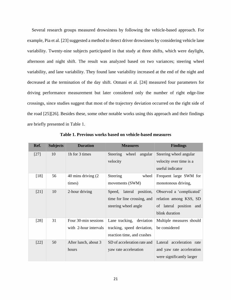
Several research groups measured drowsiness by following the vehicle-based approach. For

example, Pia et al. [23] suggested a method to detect driver drowsiness by considering vehicle lane

variability. Twenty-nine subjects participated in that study at three shifts, which were daylight,

afternoon and night shift. The result was analyzed based on two variances; steering wheel

variability, and lane variability. They found lane variability increased at the end of the night and

decreased at the termination of the day shift. Otmani et al. [24] measured four parameters for

driving performance measurement but later considered only the number of right edge-line

crossings, since studies suggest that most of the trajectory deviation occurred on the right side of

the road [25][26]. Besides these, some other notable works using this approach and their findings

are briefly presented in Table 1.

Table 1. Previous works based on vehicle-based measures

Ref. Subjects Duration Measures Findings

[27] 10 1h for 3 times Steering wheel angular

velocity

Steering wheel angular

velocity over time is a

useful indicator

[18] 56 40 mins driving (2

times)

Steering wheel

movements (SWM)

Frequent large SWM for

monotonous driving,

[21] 10 2-hour driving Speed, lateral position,

time for line crossing, and

steering wheel angle

Observed a ‘complicated’

relation among KSS, SD

of lateral position and

blink duration

[28] 31 Four 30-min sessions

with 2-hour intervals

Lane tracking, deviation

tracking, speed deviation,

reaction time, and crashes

Multiple measures should

be considered

[22] 50 After lunch, about 3

hours

SD of acceleration rate and

yaw rate acceleration

Lateral acceleration rate

and yaw rate acceleration

were significantly larger

22

Most of the studies measured many parameters during the experiment which allowed them to

access more useful information about the alertness of the operators but later worked with fewer

measures. One reason behind this is that all the recorded parameters are not equally useful as well

as some parameters showed no significant changes during operation while drowsy. However,

previous works suggest that the vehicle-based parameters are not enough to get a reliable idea

about operators' drowsy state; also the nature of the driving environment has impacts on the

recorded readings and should be considered during the study as well as for safe driving

recommendations [18]. Now, though drowsiness detection using vehicle-based measures can be

used for on-road vehicles, it is not quite suitable for aircraft. In the case of aircraft, it is reasonable

to see comparatively higher deviation in aircraft speed and track than on-road vehicles. However,

it can be used to check the extreme deviations due to drowsy flying of responsible pilots.

1.3.2 Behavioral measure

As it is mentioned earlier, drowsiness detection using vehicle-based measures is not a

reliable solution for all situations, and the outcomes of the vehicle-based research are not useful to

draw a clear relationship between drowsiness and operating properties. For these reasons, another

approach that is mainly focused on the behavior of the operator is useful since there is a significant

variation in operator’s behavior during drowsiness. Behavioral properties, especially yawning, eye

closure, blinking, head motions, percentage of eye closure (PERCLOS), hand movements, are

monitored in this method. Usually, this method uses webcam/camera and computer vision

techniques for drowsiness observation.

Comparatively more research groups worked on behavioral measures than the above-mentioned

vehicle-based measure, and the accuracy of drowsiness detection using behavioral measures is

higher than vehicle-based measures. For example, an in-flight study on 21 pilots (Air New

23

Zealand) has been conducted by Wright et al. [4] to justify the usefulness of a wrist-worn alertness

device (AD). The AD provided an auditory alarm of 95 dB when it detected wrist inactivity for at

least 5 mins. The study showed that the device was able to awaken the pilots from sleep and most

of the participants found the device acceptable to use for better safety measure.

Picot et al. [29] proposed a method to detect driver drowsiness by using visual signs, which can

be extracted from the recorded video. An algorithm was proposed that merged the useful blinking

features like PERCLOS, frequency of the blinks, amplitude-velocity ratio, and duration. The

proposed algorithm was tested for 60 hours of driving, and 20 drivers participated. The algorithm

was subject-independent and the claimed accuracy was more than 80%. Horng et al.[30] proposed

a vision-based real-time drowsiness detection method. The eye region was detected for tracking

and used for fatigue detection and an alarm was used for warning. Brandt et al. [31] presented a

visual surveillance system to track the operator’s head motion and eye blinking. The system was

able to detect fatigue and monotony, also can work in the darkness. At first, face region was

identified, and then eyes were searched in the detected face region using optical flow of the eye

region. The performance of the implemented system was tested in both simulation and natural

environments. Besides these works, Table 2 summarizes some other studies conducted using the

behavioral approach.

24

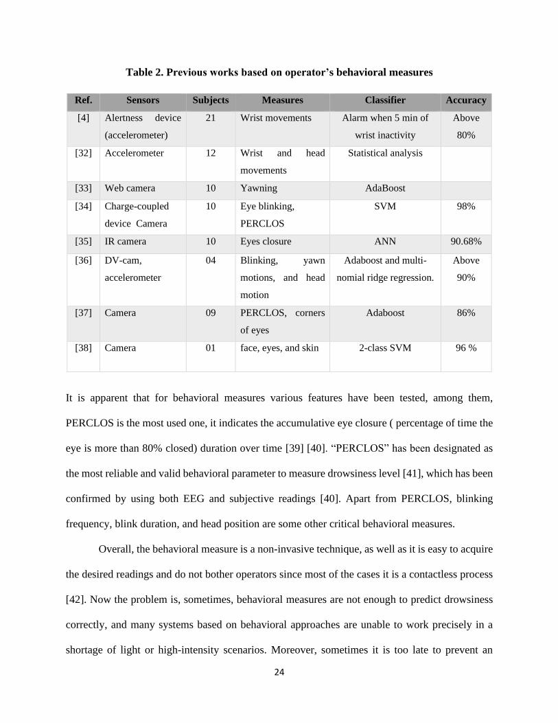
Table 2. Previous works based on operator’s behavioral measures

It is apparent that for behavioral measures various features have been tested, among them,

PERCLOS is the most used one, it indicates the accumulative eye closure ( percentage of time the

eye is more than 80% closed) duration over time [39] [40]. “PERCLOS” has been designated as

the most reliable and valid behavioral parameter to measure drowsiness level [41], which has been

confirmed by using both EEG and subjective readings [40]. Apart from PERCLOS, blinking

frequency, blink duration, and head position are some other critical behavioral measures.

Overall, the behavioral measure is a non-invasive technique, as well as it is easy to acquire

the desired readings and do not bother operators since most of the cases it is a contactless process

[42]. Now the problem is, sometimes, behavioral measures are not enough to predict drowsiness

correctly, and many systems based on behavioral approaches are unable to work precisely in a

shortage of light or high-intensity scenarios. Moreover, sometimes it is too late to prevent an

Ref. Sensors Subjects Measures Classifier Accuracy

[4] Alertness device

(accelerometer)

21 Wrist movements Alarm when 5 min of

wrist inactivity

Above

80%

[32] Accelerometer 12 Wrist and head

movements

Statistical analysis

[33] Web camera 10 Yawning AdaBoost

[34] Charge-coupled

device Camera

10 Eye blinking,

PERCLOS

SVM 98%

[35] IR camera 10 Eyes closure ANN 90.68%

[36] DV-cam,

accelerometer

04 Blinking, yawn

motions, and head

motion

Adaboost and multi-

nomial ridge regression.

Above

90%

[37] Camera 09 PERCLOS, corners

of eyes

Adaboost 86%

[38] Camera 01 face, eyes, and skin 2-class SVM 96 %

25

accident based on behavioral measures since behavioral measures are an external expression of an

internal change of physiological states, where a fatal accident may occur within a very short time

due to the sudden reduction in attention level. So, in this situation, physiological change-based

measurements are more likely to provide earlier and better detection.

1.3.3 Physiological signal-based measure

Sleepiness during flight operation is common among pilots due to long duty periods, flight

operation during the circadian low of alertness, and frequent disruption of circadian rhythm due to

time zone shift. It is worth mentioning that a previous study found that long-haul pilots use in-

flight napping as a fatigue and sleepiness countermeasure [43]. In-flight napping or having a nap

during duty periods is sometimes authorized if there is another pilot or co-pilot take control of the

aircraft. Since getting enough sleep is the only solution to reduce spontaneous sleepiness in

cockpit, it is not possible to strictly prohibit napping for pilots during a flight. Rather, introduction

of a nap schedule can be helpful to improve the vigilance level during a flight operation [44].

Therefore, the focus of these drowsiness detection systems is not to keep both pilot and co-pilot

alert when there is no apparent risk if one of them having a nap; rather, the goal of these systems

is to keep the pilot or operator alert who is in charge at that time.

Moreover, the desired devices are not intended to replace the development of rosters that

minimize fatigue and sleepiness [4]. Physiological measures based drowsiness detection focuses

on the changes of the commonly used physiological signals, such as Electroencephalography

(EEG), Electrocardiography (ECG), Electrooculography (EOG), Electromyography (EMG), and

Photoplethysmography (PPG). This method is reliable because physiological signals start to

change at an earlier stage of drowsiness, whereas behavioral and vehicular changes become

noticeable much later when preventing accidents become tough [20]. The schematic of

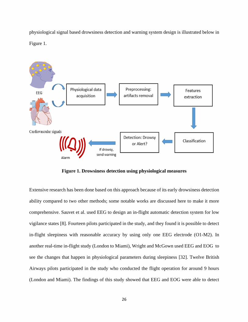
26

physiological signal based drowsiness detection and warning system design is illustrated below in

Figure 1.

Figure 1. Drowsiness detection using physiological measures

Extensive research has been done based on this approach because of its early drowsiness detection

ability compared to two other methods; some notable works are discussed here to make it more

comprehensive. Sauvet et al. used EEG to design an in-flight automatic detection system for low

vigilance states [8]. Fourteen pilots participated in the study, and they found it is possible to detect

in-flight sleepiness with reasonable accuracy by using only one EEG electrode (O1-M2). In

another real-time in-flight study (London to Miami), Wright and McGown used EEG and EOG to

see the changes that happen in physiological parameters during sleepiness [32]. Twelve British

Airways pilots participated in the study who conducted the flight operation for around 9 hours

(London and Miami). The findings of this study showed that EEG and EOG were able to detect

27

sleepiness within a short time frame (<20s), and they recommended eye movements measure as

the optimal way to monitor the onset of sleep. In another study focusing on EOG changes, Morris

and Miller found that blink amplitude, blink rate, and long closure rate were the three potential

features and can be used to measure the pilot’s vigilance state [45].

Zhang and Liu [46] studied the impact of drowsiness on ECG and pulse signals and worked

to find a natural way to monitor drowsiness. In another study, Akin et al. [47] used two other

signals EEG and EMG for observing the changes at the time of transition from wakefulness to

sleep. Both EEG and EMG were used simultaneously to increase the detection accuracy. Thirty

subjects participated in that study, and three conditions were studied for vigilance study: awake,

drowsy, and sleep. Chieh et al. [48] used EOG as a detection measure, which measured the change

of eye activities due to drowsiness. A mobile biosignal acquisition module captured the EOG

signals. Like another group (Wright and McGown) they found the EOG signal as promising to

detect drowsiness with a detection rate of 80%. In a different combination of physiological signals,

ECG and EMG were used by Sahayadhas et al. [49] for a 2-hours study at three different phases

of the day. ECG and EMG signals were recorded during driving, and the analysis of the recorded

signals was performed offline. Significant differences have been observed in the ECG and EMG

signals during the alert and drowsy period. Three signals, EEG, ECG, and EOG, were used by

Khushaba et al. [50], with a target to gather more information regarding drowsiness and to increase

the detection accuracy. Signals were acquired during the simulated driving test. The obtained

classification accuracy was 95% to 97%. Apart from these works, Table 3 summarizes some other

notable studies done in this field using physiological signal analysis.

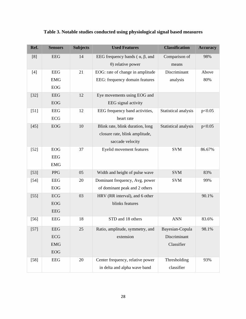
28

Table 3. Notable studies conducted using physiological signal based measures

Ref. Sensors Subjects Used Features Classification Accuracy

[8] EEG 14 EEG frequency bands ( α, β, and

θ) relative power

Comparison of

means

98%

[4] EEG

EMG

EOG

21 EOG: rate of change in amplitude

EEG: frequency domain features

Discriminant

analysis

Above

80%

[32] EEG

EOG

12 Eye movements using EOG and

EEG signal activity

[51] EEG

ECG

12 EEG frequency band activities,

heart rate

Statistical analysis p<0.05

[45] EOG 10 Blink rate, blink duration, long

closure rate, blink amplitude,

saccade velocity

Statistical analysis p<0.05

[52] EOG

EEG

EMG

37 Eyelid movement features SVM 86.67%

[53] PPG 05 Width and height of pulse wave SVM 83%

[54] EEG

EOG

20 Dominant frequency, Avg. power

of dominant peak and 2 others

SVM 99%

[55] ECG

EOG

EEG

03 HRV (RR interval), and 6 other

blinks features

90.1%

[56] EEG 18 STD and 18 others ANN 83.6%

[57] EEG

ECG

EMG

EOG

25 Ratio, amplitude, symmetry, and

extension

Bayesian-Copula

Discriminant

Classifier

98.1%

[58] EEG 20 Center frequency, relative power

in delta and alpha wave band

Thresholding

classifier

93%

29

Among the physiological signals, EEG is widely studied for drowsiness detection and sleep

disorder study [59][60]. Previous studies found that low-frequency EEG bands (within 0.5 to 13

Hz) have a substantial relationship with drowsiness [61], and regarded as reliable indices for

drowsiness detection [55]. This informative signal can be subdivided into five frequency bands,

denoted as delta band (0.5-4 Hz), theta band (4-8 Hz), alpha (8-13 Hz), the beta band (13- 30 Hz)

and gamma (>30 Hz) [62][63]. Among these, first four frequency bands (delta, theta, alpha, and

beta) are well-studied for sleep analysis. In particular, most of the drowsiness research based on

EEG is focused on the relative power variation of the theta, alpha, and beta band, as well as their

ratio indices [47][64][65]. Many of the previous studies found an inverse relationship between

alpha and beta band activity during drowsiness, alpha activity tends to increase during drowsiness,

in contrast, beta activity reduces [63][66][67][68].

ECG based heart rate variability (HRV) analysis is another measure used by many groups

for drowsy state detection. It is a measure of variations in heart rate with time and calculated by

determining beat to beat intervals ( ECG peak to peak or R to R interval) [69][70]. HRV is easy to

analysis and provides a passive way to quantify drowsiness and fatigue physiologically [71].

Individual frequency bands (such as low frequency (0.04 - 0.15 Hz) and high-frequency (0.15 -

0.40 Hz ) band) of HRV have been used for drowsiness measures [72].

1.3.4 Subjective measure

Besides these three methods of drowsiness detection, there is another approach where

subjects are directly requested to indicate his or her drowsiness level. This measure is called

subjective measure since the subject actively indicates his/her observation. Most of the time it is

used as a reference for other techniques. For subjective analysis, different scales are used by

researchers, such as Stanford Sleepiness Scale (SSS) [73][74], which had been used by some

30

groups to measure sleepiness in sleep-deprived subjects [75]. Another scale named Epworth

Sleepiness Scale (ESS) [76], used to measure the excessive daytime sleepiness in different sleep-

disordered patients [77], as well as for screening abnormalities in sleep. Profile of Mood States

(POMS) scale was used to evaluate sleepiness in different conditions [78], like sleep deprivation

[79], and work shifting [80]. Visual Analogue Scale (VAS) [81], used to measure subjective

sleepiness [82], and many research groups used this measure in their research setup [83].

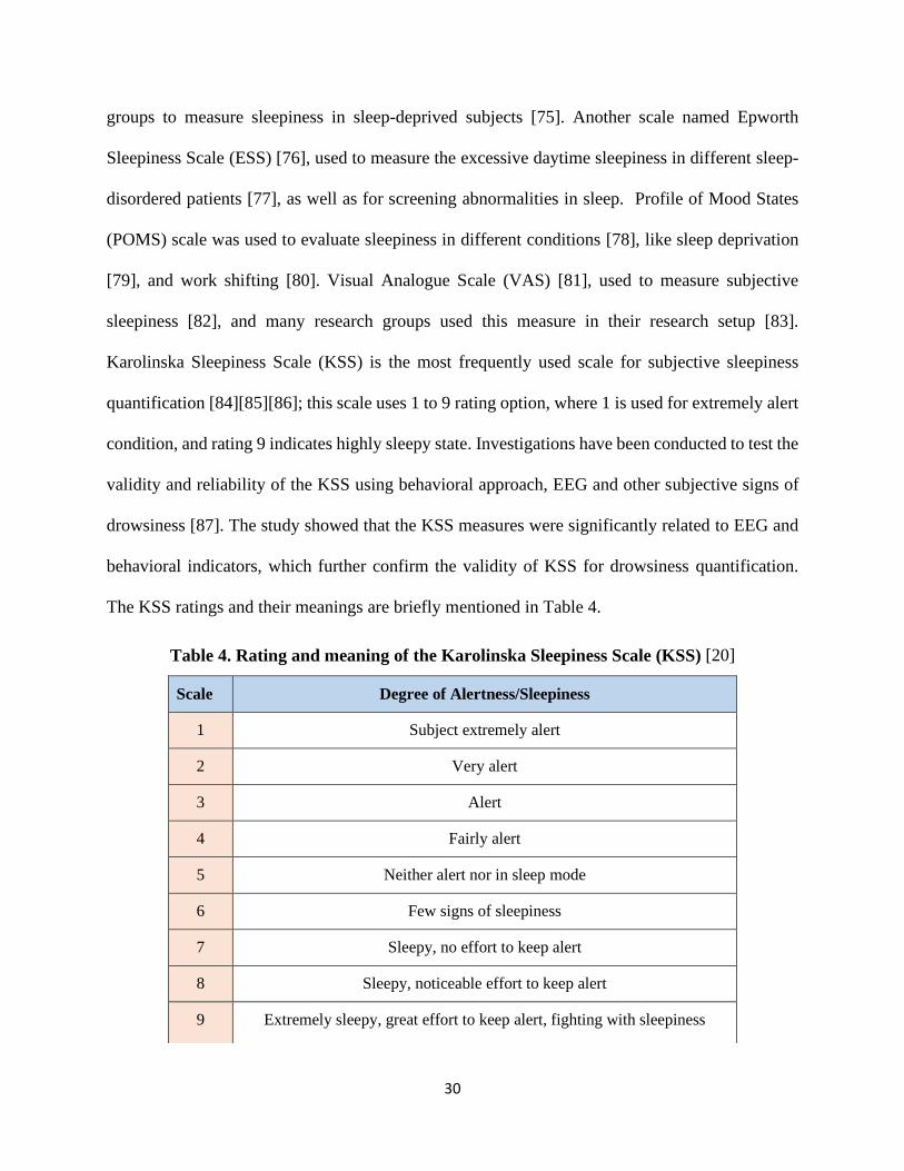
Karolinska Sleepiness Scale (KSS) is the most frequently used scale for subjective sleepiness

quantification [84][85][86]; this scale uses 1 to 9 rating option, where 1 is used for extremely alert

condition, and rating 9 indicates highly sleepy state. Investigations have been conducted to test the

validity and reliability of the KSS using behavioral approach, EEG and other subjective signs of

drowsiness [87]. The study showed that the KSS measures were significantly related to EEG and

behavioral indicators, which further confirm the validity of KSS for drowsiness quantification.

The KSS ratings and their meanings are briefly mentioned in Table 4.

Table 4. Rating and meaning of the Karolinska Sleepiness Scale (KSS) [20]

Scale Degree of Alertness/Sleepiness

1 Subject extremely alert

2 Very alert

3 Alert

4 Fairly alert

5 Neither alert nor in sleep mode

6 Few signs of sleepiness

7 Sleepy, no effort to keep alert

8 Sleepy, noticeable effort to keep alert

9 Extremely sleepy, great effort to keep alert, fighting with sleepiness

31

Usually, a subjective measure is used along with other approaches (i.e., behavioral, physiological,

or vehicle-based measure) to justify the research outcomes. Though studies on pilots found

subjective sleepiness reports were reliable for vigilance state measurement [45], a study on pilots

operating international flights found that sleep quality in prior 24h of a flight has a significant

effect on self-rated fatigue [88]. Hence, this measure is thoroughly subjective, and if measured

over a relatively long time interval, sometimes unable to provide precise measures as well as fails

to record abrupt drowsiness variation in different situations [51][61].

1.4 Simulator based Study

Simulator-based study environments are chosen most of the time over real-time studies

because real-time drowsy flying or driving experiments have a huge safety concern for both

participants and researchers. For these reasons, research groups almost always conduct their

investigations using simulators in laboratory conditions. Although there are studies that conducted

real-time studies when the subjects were operating an actual flight [51] or driving on the road,

operating with sleepiness is only safe in controlled setup used for simulation-based study [89]. The

simulators are specialized systems where a realistic route is displayed by using projectors or

computer monitors, and the aircraft movement is controlled using controllers similar to real aircraft

or using wheel used for driving [90]. It allows the operator to immerse himself/herself in a real-

life condition, also provides an opportunity for the investigators to inspect their algorithms [35].

Modern simulators use more than one projector and able to provide an almost 360-degree realistic

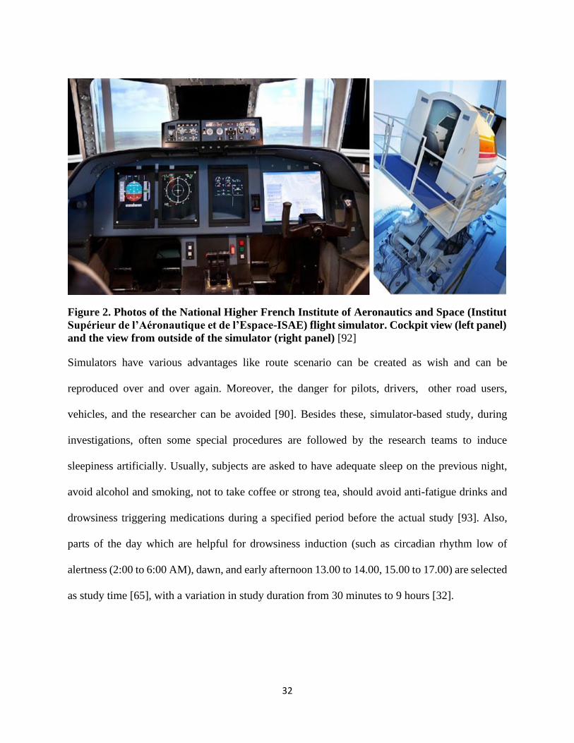
visual display with a combination of various scenarios [91]. Figure 2 shows a snap of an aircraft

simulator used for a study [92].

32

Simulators have various advantages like route scenario can be created as wish and can be

reproduced over and over again. Moreover, the danger for pilots, drivers, other road users,

vehicles, and the researcher can be avoided [90]. Besides these, simulator-based study, during

investigations, often some special procedures are followed by the research teams to induce

sleepiness artificially. Usually, subjects are asked to have adequate sleep on the previous night,

avoid alcohol and smoking, not to take coffee or strong tea, should avoid anti-fatigue drinks and

drowsiness triggering medications during a specified period before the actual study [93]. Also,

parts of the day which are helpful for drowsiness induction (such as circadian rhythm low of

alertness (2:00 to 6:00 AM), dawn, and early afternoon 13.00 to 14.00, 15.00 to 17.00) are selected

as study time [65], with a variation in study duration from 30 minutes to 9 hours [32].

Figure 2. Photos of the National Higher French Institute of Aeronautics and Space (Institut

Supérieur de l’Aéronautique et de l’Espace-ISAE) flight simulator. Cockpit view (left panel)

and the view from outside of the simulator (right panel) [92]

33

1.5 Discussion

Based on the review of previous works it is clear that the vehicle-based approach is not quite

feasible for aircraft due to the frequent variation in aircraft speed and deviation from the desired

route compared to on-road vehicles, which are all counted as reasonable for aviation. However,

extreme deviation from the desired route, change of direction, and change in altitude can be used

as features, though extensive research required to check their capability and usability.

Although the behavioral approach is easy to apply for real-time applications due to being

contactless or using less body contact, they are not reliable enough compared to physiological

signal-based approach and unable to provide early warning. Hence, the physiological signal-based

approach is the better option since it has a close relation with the internal states of the body and

able to provide an earlier warning before drowsiness interrupts operation. However, to make it

applicable for the real-time applications there is a necessity to facilitate less intrusive and

comfortable physiological data acquisition.

34

CHAPTER 02

METHODOLOGY

As discussed earlier, physiological signal-based approach has the potential to predict

drowsiness earlier with better accuracy compared to two other methods. So, in this research work,

the focus was to detect drowsiness using some of the commonly used physiological signals.

2.1 Commonly used Physiological Signals

The physiological signals which are commonly studied for drowsiness detection are

Electrocardiogram (ECG)

Electroencephalogram (EEG)

Electrooculogram (EOG)

Photoplethysmography (PPG)

Electromyogram (EMG)

2.1.1 Electrocardiogram (ECG)

The heart is a vital organ that pumps blood throughout the body using the body circulatory

system, it supplies oxygen and nutrients to the tissues and removes carbon dioxide and other wastes

produced by the tissues [94]. It can pump more than 6000 liters of blood each day continuously

during the whole life period and beats around 40 million times per year [95]. The heart has four

chambers: two atria (upper chambers) and two ventricles (lower chambers). The right atrium and

the right ventricle together make up the “right heart” whereas the left atrium and the left ventricle

make up the “left heart.” A muscle wall named the septum between the two sides of the heart

works as a separator [94][96]. The right atrium receives the deoxygenated blood from the body

and sends it to the right ventricle. The right ventricle then pumps the oxygen poor blood to the

35

lungs, where the blood gets purified and oxygenated. The oxygen-rich blood then goes to the left

atrium, and it pumps the blood to the left ventricle. The left ventricle finally pumps the oxygen-

rich blood to the body through the body circulatory system [97]. The atria and ventricles work

together, periodically contract and relax to pump blood throughout the body. The electrical system

of the heart is the power source, which makes it possible. Each heartbeat is triggered by an

electrical impulse that travels through a special pathway down to the heart. The sinoatrial node

(SA node), a small bundle of specialized cells located in the right atrium is the source of this

electrical impulse [98]. The SA node is known as the natural pacemaker of the heart. The electrical

activity then spreads throughout the walls of the right atrium and left atrium and triggers them to

contract. The contraction of both atrium then push their blood into the right and left ventricle [99].

The atrioventricular node (AV node) is a bundle of cells in the center of the heart, situated

between the atria and ventricles. The AV node works like a gate, which slows down the electrical

impulse before it travels to the ventricles which in turn provides time to both right and left atrium

to contract before ventricle contraction starts. The His-Purkinje fibers then conduct the electrical

impulse to the muscular wall of the two ventricles and trigger them to contract. The contraction of

the muscles of the ventricles results in pushing the blood out of the heart to the lungs (from the

right ventricle) and body (from the left ventricle) [98].

However, when the electric signal travels through the heart, there are changes in voltage

which can be detected by placing/attaching electrodes on the chest, which are then graphed, and

this process of recording is known as electrocardiography (ECG), also known as 12-lead ECG, or

EKG. This is a non-invasive test, and the acquired record is known as an electrocardiogram (ECG),

which helps to know about the heart rhythm, heart diseases, frequency, action, and the position of

the heart [95][99]. A typical ECG waveform is shown below.

36

Figure 3. A normal Electrocardiogram tracing [96]

The P wave represents the depolarization of the right and left atrium, whereas the short duration

QRS complex represents the ventricular (right and left ventricle) depolarization. The T wave

represents the ventricular repolarizations [100].

2.1.2 Electroencephalogram (EEG)

The brain is the most complex organ of the human body. It works like the command center

for the human nervous system. The outermost layer of the brain is known as the cerebral cortex,

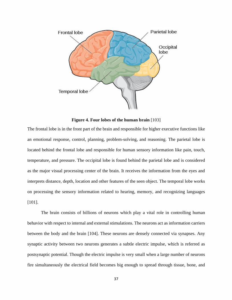
which gives it the wrinkly characteristics [101]. The cerebral cortex is lengthwise divided into two

subsections, one is the left hemisphere, and another is the right hemisphere. Each hemisphere is

then subdivided into four lobes, named, frontal, parietal, occipital, and temporal lobe [101][102].

37

Figure 4. Four lobes of the human brain [103]

The frontal lobe is in the front part of the brain and responsible for higher executive functions like

an emotional response, control, planning, problem-solving, and reasoning. The parietal lobe is

located behind the frontal lobe and responsible for human sensory information like pain, touch,

temperature, and pressure. The occipital lobe is found behind the parietal lobe and is considered

as the major visual processing center of the brain. It receives the information from the eyes and

interprets distance, depth, location and other features of the seen object. The temporal lobe works

on processing the sensory information related to hearing, memory, and recognizing languages

[101].

The brain consists of billions of neurons which play a vital role in controlling human

behavior with respect to internal and external stimulations. The neurons act as information carriers

between the body and the brain [104]. These neurons are densely connected via synapses. Any

synaptic activity between two neurons generates a subtle electric impulse, which is referred as

postsynaptic potential. Though the electric impulse is very small when a large number of neurons

fire simultaneously the electrical field becomes big enough to spread through tissue, bone, and

38

skull. Eventually, can be measured on the head surface or skin [105][106]. Electroencephalography

(EEG) is the physiological method used to record this electrical activity generated by thousands of

neurons in the brain by placing electrodes on the scalp. Simply, EEG is a record of the electrical

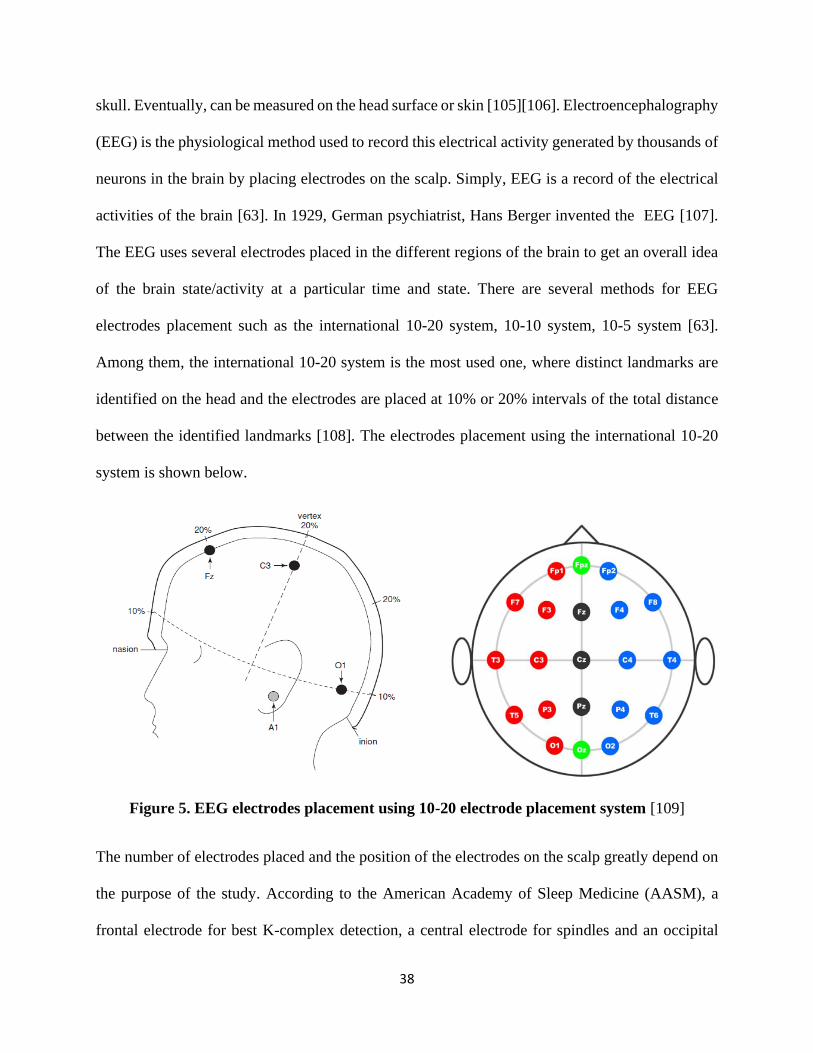
activities of the brain [63]. In 1929, German psychiatrist, Hans Berger invented the EEG [107].

The EEG uses several electrodes placed in the different regions of the brain to get an overall idea

of the brain state/activity at a particular time and state. There are several methods for EEG

electrodes placement such as the international 10-20 system, 10-10 system, 10-5 system [63].

Among them, the international 10-20 system is the most used one, where distinct landmarks are

identified on the head and the electrodes are placed at 10% or 20% intervals of the total distance

between the identified landmarks [108]. The electrodes placement using the international 10-20

system is shown below.

Figure 5. EEG electrodes placement using 10-20 electrode placement system [109]

The number of electrodes placed and the position of the electrodes on the scalp greatly depend on

the purpose of the study. According to the American Academy of Sleep Medicine (AASM), a

frontal electrode for best K-complex detection, a central electrode for spindles and an occipital

39

electrode for alpha wave should be placed for the visual scoring purpose. They recommended a

frontal electrode Fz, a central one C4, and an occipital one O1. Also, F4, C3, Cz, and O2 are

recommended to use in case any electrode falls off or not working properly [108][109].

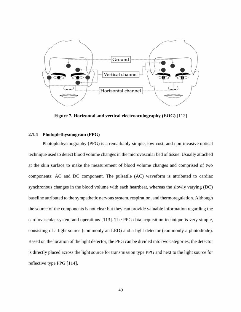
2.1.3 Electrooculogram (EOG)

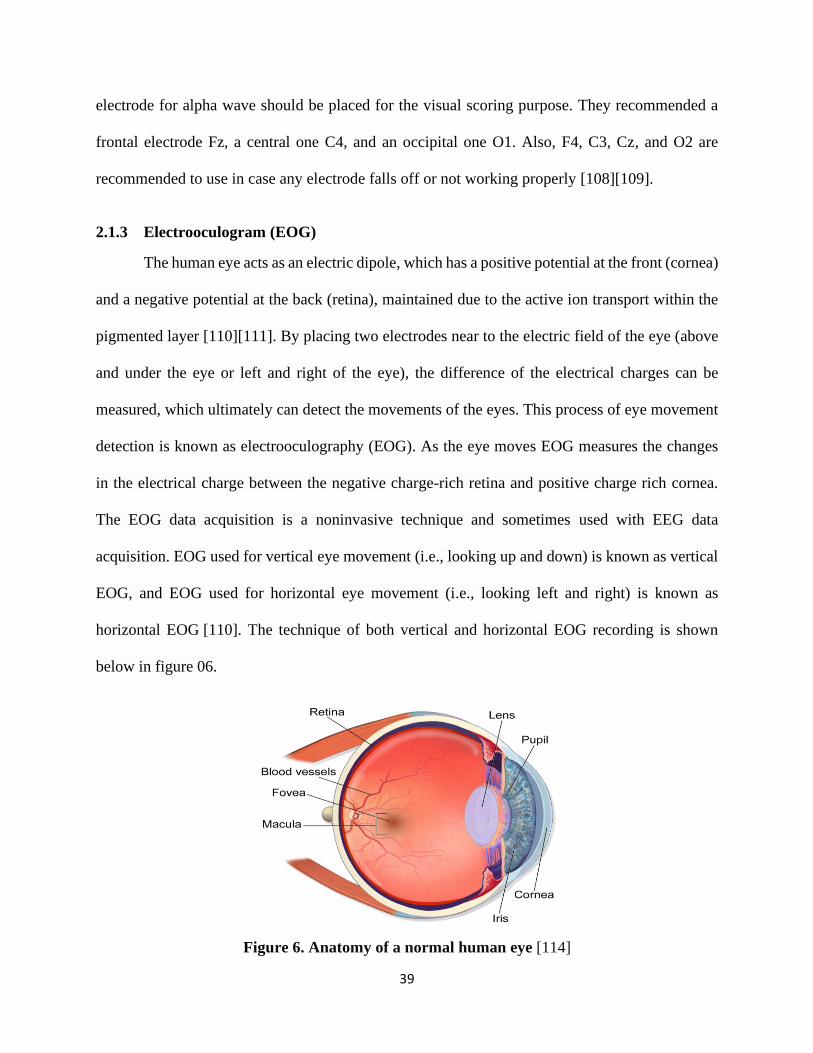
The human eye acts as an electric dipole, which has a positive potential at the front (cornea)

and a negative potential at the back (retina), maintained due to the active ion transport within the

pigmented layer [110][111]. By placing two electrodes near to the electric field of the eye (above

and under the eye or left and right of the eye), the difference of the electrical charges can be

measured, which ultimately can detect the movements of the eyes. This process of eye movement

detection is known as electrooculography (EOG). As the eye moves EOG measures the changes

in the electrical charge between the negative charge-rich retina and positive charge rich cornea.

The EOG data acquisition is a noninvasive technique and sometimes used with EEG data

acquisition. EOG used for vertical eye movement (i.e., looking up and down) is known as vertical

EOG, and EOG used for horizontal eye movement (i.e., looking left and right) is known as

horizontal EOG [110]. The technique of both vertical and horizontal EOG recording is shown

below in figure 06.

Figure 6. Anatomy of a normal human eye [114]

40

Figure 7. Horizontal and vertical electrooculography (EOG) [112]

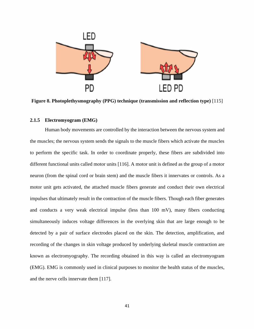
2.1.4 Photoplethysmogram (PPG)

Photoplethysmography (PPG) is a remarkably simple, low-cost, and non-invasive optical

technique used to detect blood volume changes in the microvascular bed of tissue. Usually attached

at the skin surface to make the measurement of blood volume changes and comprised of two

components: AC and DC component. The pulsatile (AC) waveform is attributed to cardiac

synchronous changes in the blood volume with each heartbeat, whereas the slowly varying (DC)

baseline attributed to the sympathetic nervous system, respiration, and thermoregulation. Although

the source of the components is not clear but they can provide valuable information regarding the

cardiovascular system and operations [113]. The PPG data acquisition technique is very simple,

consisting of a light source (commonly an LED) and a light detector (commonly a photodiode).

Based on the location of the light detector, the PPG can be divided into two categories; the detector

is directly placed across the light source for transmission type PPG and next to the light source for

reflective type PPG [114].

41

Figure 8. Photoplethysmography (PPG) technique (transmission and reflection type) [115]

2.1.5 Electromyogram (EMG)

Human body movements are controlled by the interaction between the nervous system and

the muscles; the nervous system sends the signals to the muscle fibers which activate the muscles

to perform the specific task. In order to coordinate properly, these fibers are subdivided into

different functional units called motor units [116]. A motor unit is defined as the group of a motor

neuron (from the spinal cord or brain stem) and the muscle fibers it innervates or controls. As a

motor unit gets activated, the attached muscle fibers generate and conduct their own electrical

impulses that ultimately result in the contraction of the muscle fibers. Though each fiber generates

and conducts a very weak electrical impulse (less than 100 mV), many fibers conducting

simultaneously induces voltage differences in the overlying skin that are large enough to be

detected by a pair of surface electrodes placed on the skin. The detection, amplification, and

recording of the changes in skin voltage produced by underlying skeletal muscle contraction are

known as electromyography. The recording obtained in this way is called an electromyogram

(EMG). EMG is commonly used in clinical purposes to monitor the health status of the muscles,

and the nerve cells innervate them [117].

42

However, EMG is used by some of the research groups to detect or quantify the drowsiness during

driving [49]. Mainly EMG is used to see the changes in muscle behavior during drowsiness or

impaired attention level compared to alert periods. Usually, trapezius muscles are targeted for

drowsiness monitoring since there is a significant change in these muscle bundles during

drowsiness and head movements [118].

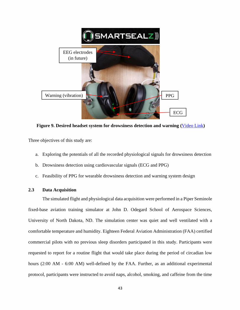
2.2 Our System

The goal of this project (Smartsealz) is to design a headset like device (commonly used by

the pilots) with physiological data acquisition, analysis capability, and feedback facility, which

can provide warning whenever a drowsy state is detected. Three physiological signals, ECG, PPG

(ear), and EEG were recorded simultaneously, where the cardiovascular signals (ECG and PPG)

are used to check their applicability for the desired system, and EOG was recorded as a gold

standard of eye closure measure. The idea is to incorporate the ECG, PPG sensor and a haptic

warning system in the headset ear pad (see Figure 9). Whereas informative EEG electrodes can be

positioned in the headband as well (in the future). The desired system should not be uncomfortable

for the aircraft pilots since they are already used to this headset mainly used for communication

with Air Traffic Control (ATC) and noise cancellation. However, with a simpler design, the

headset can be useful for on-road applications as well, which will help to avoid many accidents

occur due to drowsy driving.

43

Figure 9. Desired headset system for drowsiness detection and warning (Video Link)

Three objectives of this study are:

a. Exploring the potentials of all the recorded physiological signals for drowsiness detection

b. Drowsiness detection using cardiovascular signals (ECG and PPG)

c. Feasibility of PPG for wearable drowsiness detection and warning system design

2.3 Data Acquisition

The simulated flight and physiological data acquisition were performed in a Piper Seminole

fixed-base aviation training simulator at John D. Odegard School of Aerospace Sciences,

University of North Dakota, ND. The simulation center was quiet and well ventilated with a

comfortable temperature and humidity. Eighteen Federal Aviation Administration (FAA) certified

commercial pilots with no previous sleep disorders participated in this study. Participants were

requested to report for a routine flight that would take place during the period of circadian low

hours (2:00 AM - 6:00 AM) well-defined by the FAA. Further, as an additional experimental

protocol, participants were instructed to avoid naps, alcohol, smoking, and caffeine from the time

EEG electrodes

(in future)

PPG

suroji

t.gupt

a@U

ND.e

du

Warning (vibration)

ECG

suroji

t.gupt

a@U

ND.e

du

44

they woke up in the previous day in advance of appearing for the study at midnight (around 01:30

AM). Each participant’s data acquisition was subdivided into two phases: a take-off phase of

approximately 6 minutes and a cruise phase (autopilot activation allowed) of about 2 hours. The

data acquisition process was approved by the Institutional Review Board (IRB) of the University

of North Dakota. The participants had signed an informed consent form before starting the study.

The data acquisition sessions were concluded upon meeting one of the three conditions: (1) the

simulated flight course reached at least 2.5 hours of flight time, (2) the subject had been awoken

by the researchers twice during sleeping with a duration of more than five minutes, (3) the subject

himself/herself decided to discontinue the data recording session [11][119]. Table 6 represents the

general information about all the subjects who participated in this study; subject IDs were

randomly selected.

Table 5. Information of participants. A significant difference was observed in the KSS

value at the end of the study compared to the beginning. ‘*’ represents alpha level at 0.05

Subject

ID

Age

(years)

Gender Flight

Time

(hours)

Takeoff

time

(am)

End

Time

(am)

KSS

(start)

KSS

(end)

105 20 Male 250 2:04 4:26 6.0 9.0

122 27 Male 400 2:14 4:21 6.0 8.0

126 21 Male 280 2:11 4:11 7.0 8.0

133 21 Male 315 2:11 4:18 4.0 9.0

135 28 Male 419 1:57 4:04 6.0 9.0

136 21 Female 185 2:08 4:08 7.0 9.0

140 21 Male 200 2:06 3:25 7.0 9.0

143 20 Male 400 2:06 4:18 7.0 9.0

145 20 Male 430 2:10 4:15 6.0 8.0

149 21 Male 200 2:09 4:23 3.0 8.0

165 21 Male 215 2:00 4:26 3.0 9.0

172 20 Male 280 2:05 4:20 7.0 9.0

179 21 Male 250 2:09 4:33 4.0 8.0

183 21 Male 300 2:13 3:42 7.0 9.0

198 21 Female 195 2:20 4:06 5.0 9.0

199 20 Male 200 2:08 4:15 1.0 9.0

Mean 21.5±2.4 14 / 2 282±87 2:08 4:11 5.4±1.9 8.7±0.5*

45

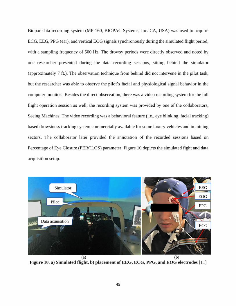
Biopac data recording system (MP 160, BIOPAC Systems, Inc. CA, USA) was used to acquire

ECG, EEG, PPG (ear), and vertical EOG signals synchronously during the simulated flight period,

with a sampling frequency of 500 Hz. The drowsy periods were directly observed and noted by

one researcher presented during the data recording sessions, sitting behind the simulator

(approximately 7 ft.). The observation technique from behind did not intervene in the pilot task,

but the researcher was able to observe the pilot’s facial and physiological signal behavior in the

computer monitor. Besides the direct observation, there was a video recording system for the full

flight operation session as well; the recording system was provided by one of the collaborators,

Seeing Machines. The video recording was a behavioral feature (i.e., eye blinking, facial tracking)

based drowsiness tracking system commercially available for some luxury vehicles and in mining

sectors. The collaborator later provided the annotation of the recorded sessions based on

Percentage of Eye Closure (PERCLOS) parameter. Figure 10 depicts the simulated fight and data

acquisition setup.

(a) (b)

Figure 10. a) Simulated flight, b) placement of EEG, ECG, PPG, and EOG electrodes [11]

Simulator

Pilot

Data acquisition

EEG

ECG

PPG

EOG

46

However, drowsy periods annotated in this way (i.e., based on PERCLOS and direct observation)

were further validated by manual observation of the EOG signal that no blink was witnessed in

those periods. Some of the events which disagreed with the PERCLOS and direct observation-

based annotations were later disregarded for analysis. There were many sleepy events less than

15s (Seeing Machines named these periods as Microsleeps), as well as greater than 15s, with a

duration as long as 4-5 minutes (Seeing Machines named these periods as Longsleeps).

We used different lengths of periods for different aspects of the study which are described

later. For example, for heart rate variability (HRV) analysis, different segment lengths varying

from commonly used 5 min, 3 min, to 120s, and 30s for ultra-short HRV measurement were used.

For pulse arrival time (PAT) and PPG feature analysis, the focus was on drowsy periods greater

than 15s and less than 35s based on the EOG analysis. Since it is unusual for a person to keep

his/her eyes open for more than this period without any blink considering a normal blinking

frequency of 15-20 times per minute [120], this consideration allowed us a natural interpretation

of EOG and aggregation of a significant number of drowsy periods. Moreover, much shorter

duration drowsy periods (less than 5s) were not suitable for getting a reliable PAT due to the very

few numbers of ECG and PPG waveforms.

As mentioned earlier, the take-off and climb phase was roughly 6 minutes, when the pilots

were manually operating the flight simulator. Therefore, the participants were more engaged (i.e.,

comparatively alert) during this period. On the other hand, after the take-off phase, pilots were

allowed to activate the “autopilot” which reduced interaction with aircraft control. The use of the

autopilot combined with operations during the window of circadian low facilitated the opportunity

for observation of sleepy periods. These periods of reduced wakefulness were selected from the

whole recording of around 2 hours, while baseline or alert periods were selected within the first

47

12 minutes of the recording. Considering noise and excessive moving artifacts, the first 3 minutes

were excluded from the baseline, so the actual baseline considered here was within the range of 3

to 12 minutes of the beginning of the recording session.

2.4 Data Analysis

ECG and PPG signals were filtered with a high pass filter of 0.5 Hz cut-off frequency to

remove the baseline and later filtered with a 60 Hz notch filter to remove the power line noise

[121]. PPG signals are significantly vulnerable to physiological (e.g., respiration, head tilt) and

measurement (e.g., motion) oriented artifacts [115] [122]. So, PPG signals were further filtered

with a low pass filter of cut off frequency of 10 Hz [123]. The used filters did not add any phase

shifts in the original signals.

The R-peaks of the ECG signal were detected by using the Pan-Tompkins algorithm [124].

Then RR intervals were calculated using the distance between consecutive R-peaks. These RR

intervals were later used to measure heart rate and different heart rate variability (HRV) parameters

as shown in Tables 2 and 3. As it is known, a PPG pulse is observed within consecutive R peaks

of the ECG waveform, the R-peaks location obtained from the Pan-Tompkins algorithm were used

to locate the PPG waveform peaks. These PPG peaks (P-peak) were used to calculate the PP

intervals (like RR intervals). Later, PP intervals were used to calculate different pulse rate

variability (PRV) parameters. Distance between the ECG R peak and the PPG peak, foot, first

derivative peak, and second derivative peak were calculated to determine the pulse arrival time

(PAT) during the drowsy and baseline periods [11].

Each subject had to fulfill two conditions to be counted for PAT analysis, which were:

(a) Good PPG and ECG (i.e., less distortion in each cycle) signal in both baseline and drowsy

periods

48

(b) Has at least one drowsy period greater than 15s

Four methods were used for pulse arrival time calculation using ECG R peaks and PPG waveform:

(a) Using the lowest point (foot) of PPG waveform

(b) Peak values of PPG waveforms

(c) The peak value of the first derivative of PPG

(d) The peak value of the second derivative of PPG

In case of EEG analysis, power spectral density (PSD) analysis was used to measure the changes

in band power in four EEG frequency bands (delta (0.5-4Hz), theta (4-8Hz), alpha (8-13Hz), and

beta (13-30Hz)) during drowsiness (microsleeps and longsleeps) compared to alert periods [63].

Among 18 subjects recorded initially, Subject 173 data recording was interrupted due to a

technical issue, Sub. 136 had finger PPG due to problems with ear PPG, Sub. 140, 143, 149, and

198 had bad PPG or ECG signals either in drowsy periods or baseline periods. As a result, these

six subjects were excluded from our PAT analysis. Therefore, 12 subjects had been used for PAT

analysis [11]. Whereas for heart rate variability (HRV) and pulse rate variability (PRV)

measurement number of subjects included in the analysis varied based on the sleepy periods, for

example, 10 subjects were included in the study for HRV measurement using 5 min window since

other subjects did not have significant drowsy periods in this range. Fifteen subjects were used for

HRV analysis before the first drowsy period, 10 subjects were used for the ultra-short (30s) HRV

analysis, and 12 subjects were used for only PPG based feature extraction due to bad PPG signal

of some of the subjects. Besides, sixteen subjects were used for EEG spectral analysis.

49

2.5 Discussion

Physiological signal-based approach appeared as a suitable option for pilots’ drowsiness

detection due to its ability to provide earlier prediction and better detection accuracy. Since EEG

provides insights about brain function, it is the most commonly used physiological signal in this

purpose. However, the problem with EEG is that EEG data acquisition requires many electrodes

placed on the scalp which is not feasible for real-time on-board applications. By identifying

informative brain regions for drowsiness quantification, it is possible to reduce the number of

electrodes and it will be beneficial for real-time applications.

However, based on previous studies, both ECG and PPG appear to be promising in

discriminating between alert and drowsy periods. Further, they need fewer electrodes compared to

EEG, which is advantageous for on-board applications. Hence, instead of depending on only one

signal it is better to use a combination of signals which can provide a better detection accuracy

with reduced false positive rate. The goal of this study was to explore the potentials of these

physiological signals (especially ECG and PPG), whether they can significantly differentiate

between drowsy periods and alert periods.

50

CHAPTER 03

RESULTS

Analyses for drowsiness detection based on physiological signals are mainly focused on

heart rate variability (HRV) analysis using ECG signal, pulse rate variability (PRV) analysis using

PPG signal, HRV and PRV agreement comparison, pulse arrival time (PAT) calculation using

PPG and ECG, features based on PPG, and power spectral density (PSD) analysis of EEG bands.

For HRV analysis, different time domain and frequency domain features have been extracted with

a variation of the time window varying from commonly used 5-minute window to 30s- window

(ultrashort HRV). The same was followed for PRV analysis as well. For PAT analysis (time

interval between ECG R peak and any specific point of PPG waveform), four methods of PAT

calculation i.e., PPG peak, PPG foot, the first derivative peak of PPG signal, and the second

derivative peak of PPG were followed. For only PPG based features, PPG width, timing, and

height-based features were extracted from each PPG pulse and compared for both baseline and

drowsy periods.

3.1 Heart Rate Variability (HRV) Analysis

Heart rate variability (HRV) is the variation in the duration or length of heartbeat intervals

[125]. It is a noninvasive method and reflects the capability of the heart to respond to various

psychophysiological and environmental stimuli. HRV provides a powerful way of observing the

interrelation between the sympathetic and parasympathetic nervous system activities. [126].

HRV is controlled by the autonomic nervous system (ANS), and it’s two branches named the

sympathetic nervous system (SNS) and parasympathetic nervous system (PNS). The sympathetic

branch is the stress, exercise, or fight or flight system and helps us to act quickly, react, and perform

51

when required. On the other hand, the parasympathetic system is denoted as the rest and digest

system, which allows the body to power down and recover after the reduction of the sympathetic

activity or when there is no necessity for a quick response. The sympathetic system activates stress

hormone production, which results in the heart’s increased contraction rate (i.e., increased heart

rate) and force (cardiac output), as a result, decreased HRV during exercise, and physically or

mentally challenging/stressful conditions. On the other hand, the parasympathetic system reduces

heart rate and increases HRV to restore homeostasis when there is less or no stress or mentally

challenging task performance required [126][127]. The separate contributions from sympathetic

and parasympathetic activity modulate the heart rate, i.e., RR intervals of the QRS complex in the

electrocardiogram at different frequencies. Sympathetic activity is related to a low-frequency

range (0.04 to 0.15 Hz), whereas parasympathetic activity is related to the higher frequency range

(0.15 to 0.4 Hz) of modulation frequencies of heart rate. Based on the activity in specific frequency

range it is possible to separate sympathetic and parasympathetic activity domination in HRV

analysis [126].

Figure 11. RR interval variation [129]

52

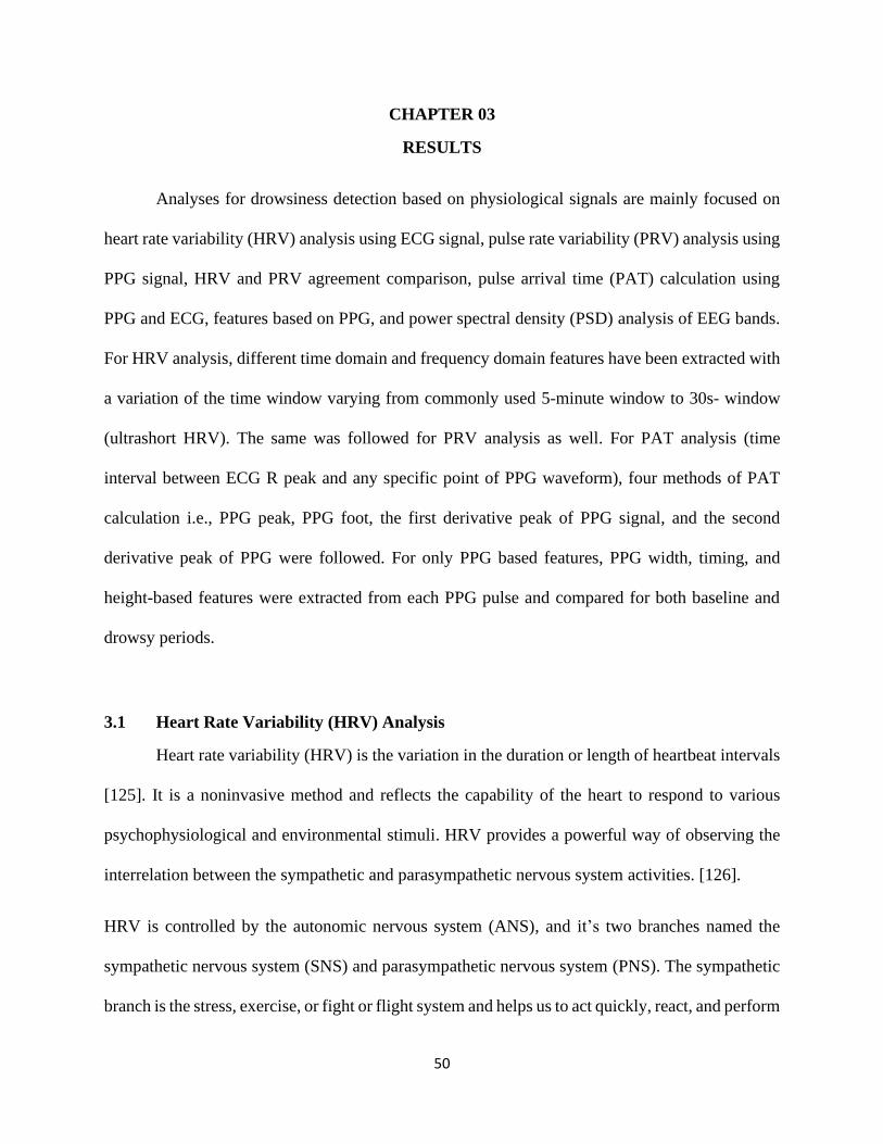
Figure 12. Heart rate variability over 24 hours [121]

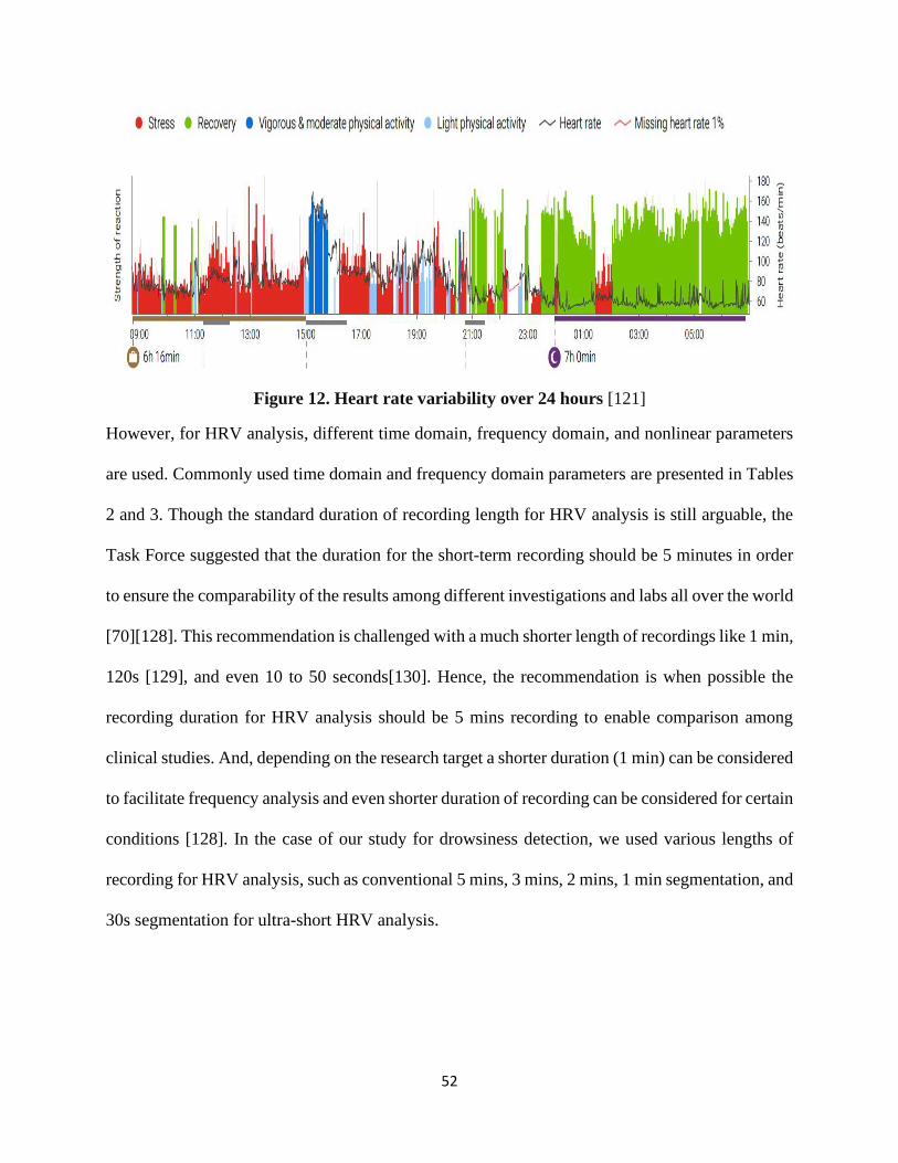
However, for HRV analysis, different time domain, frequency domain, and nonlinear parameters

are used. Commonly used time domain and frequency domain parameters are presented in Tables

2 and 3. Though the standard duration of recording length for HRV analysis is still arguable, the

Task Force suggested that the duration for the short-term recording should be 5 minutes in order

to ensure the comparability of the results among different investigations and labs all over the world

[70][128]. This recommendation is challenged with a much shorter length of recordings like 1 min,

120s [129], and even 10 to 50 seconds[130]. Hence, the recommendation is when possible the

recording duration for HRV analysis should be 5 mins recording to enable comparison among

clinical studies. And, depending on the research target a shorter duration (1 min) can be considered

to facilitate frequency analysis and even shorter duration of recording can be considered for certain

conditions [128]. In the case of our study for drowsiness detection, we used various lengths of

recording for HRV analysis, such as conventional 5 mins, 3 mins, 2 mins, 1 min segmentation, and

30s segmentation for ultra-short HRV analysis.

53

Table 6. Commonly used time-domain parameters for HRV analysis [70] [131]

Variables Units Description

RR milliseconds

(ms)

ECG R peak to R peak interval

SDNN ms The standard deviation of all RR intervals (also known as NN intervals)

SDSD ms Standard deviation of differences between adjacent RR intervals

SDANN ms Standard deviation of the averages of RR intervals in all segments of the

entire recording

RMSSD ms Root mean square of the successive differences (i.e., the square root of

the mean of the sum of the squares of the differences between adjacent

RR intervals)

SDNN

Index

ms Mean of the standard deviations of all RR intervals for all segments of

the entire recording

NN50 count Number of pairs of adjacent RR intervals differing by more than 50 ms

in that segment or the entire recording. Three variants are possible

counting all such RR interval pairs, or only pairs where the first one or

the second one is greater

pNN50 % NN50 count divided by the total number of all NN pairs

Table 7. Commonly used frequency domain parameters for HRV analysis [70] [131]

Variables Units Description Frequency range

Short time segments (5 min, 3 min)

VLF ms2 Absolute power in very low frequency range ≤0.04 Hz

LF ms2 Absolute power in low frequency range 0.04 to 0.15 Hz

HF ms2 Absolute power in high frequency range 0.15 to 0.4 Hz

LF

normalized

or LF (%)

n.u. or

%

Relative power in normalized unit or

(LF/ total power)*100

HF

normalized

or HF (%)

n.u. or

%

Relative power in normalized unit or

(HF/ total power)*100

Total power ms2 The variance of RR intervals over the segment Within in ≤ 0.4 Hz

LF/HF Ratio of LF and HF

For 24h recording

ULF ms2 Absolute power in the ultra-low frequency range ≤0.003 Hz

VLF ms2 Absolute power in very-low frequency range 0.003 to 0.04 Hz

54

LF ms2 Absolute power in low frequency range 0.04 to 0.15 Hz

HF ms2 Absolute power in high frequency range 0.15 to 0.4 Hz

Total power ms2 Variance of all RR intervals within the segment ≤ 0.4 Hz

∞ Slope of the linear interpolation of the spectrum in

a log-log scale

approximately ≤0.04

Hz

3.1.1 HRV using 5 min windowing

HRV analysis had been performed using 5 min (300s) windowing, with 50% overlapping

and 1-second progression. Commonly used time-domain features (i.e., HR, SDNN, SDSD,

RMSSD, NN50, and PNN50) and frequency domain features (i.e., VLF, LF, HF, and LF/HF) were

calculated for baseline and drowsy periods (including both microsleep (10-15s) and longsleep

(>16s)). Then the feature values were compared for two classes to check the significant changes.

Among the 10 features, SDNN, SDSD and RMSSD showed significant (p<0.05, two sample t-

test) change during drowsy periods compared to baseline periods. Tables 4 to 7 represent the

feature values (Mean±Std) calculated using 5 min windowing.

Table 8. Comparison of Heart rate, SDNN, and SDSD

Heart rate SDNN SDSD

Subs. Baseline

(Mean±Std)

Drowsy

(Mean±Std)

Baseline

(Mean±Std)

Drowsy

(Mean±Std)

Baseline

(Mean±Std)

Drowsy

(Mean±Std)

105 73.2±0.5 70.5±0.6 127.2±8 169.9±9. 2 183.8±17.5 242.6±17.8

122 73.0±0. 72.9±0.2 53.35±3.6 60.9±5. 5 54.9±9.3 63.6±12.6

133 78.5±0.3 78.2±0.3 94.4±13.2 101.0±8. 5 132.7±21.3 143.8±13.8

135 64.7±0.3 63.5±0.2 81.0±2.7 73.8±3. 0 73.7±6.5 68.3±5.2

140 80.8±0.3 77.3±0.4 121.8±9.9 206.5±7. 9 174.9±15.4 308.6±14.3

143 75.0±0.4 70.7±0.5 116.5±8.5 187.6±8. 2 162.3±17.0 250.6±16.4

145 97.4±1.0 86.0±0.2 132.7±13.1 255.9±1.9 194±25.9 409.1±5.1

165 88.3±0.3 83.0±0.3 113.9±12.1 231.7±4.3 162.1±17.2 346.6±7.6

179 91.3±0.7 80.3±0.3 134.1±18.3 284.5±3. 1 191.8±28.2 439±7.2

183 82.1±0.3 81.1±0.3 91.6±14.1 135.2±8.9 128.3±20.6 194.5±12.9

Mean 80.4±0.4 76.3±0.3 106.7±10.3 170.7±6. 1 145.9±17.9 246.7±11.3

55

Table 9. Comparison of NN50, PNN50, and RMSSD

Table 10. Comparison of VLF(%), LF(%) and HF(%)

Table 11. Comparison of LF/HF

NN50 PNN50 RMSSD

Subs. Baseline

(Mean±Std)

Drowsy

(Mean±Std)

Baseline

(Mean±Std)

Drowsy

(Mean±Std)

Baseline

(Mean±Std)

Drowsy

(Mean±Std)

105 79.9±3.6 45.9±2.8 0.3±0.0 0.3±0.0 183.6±17.5 241.9±17.7

122 12.2±1.8 10.9±2.3 0.04±0.0 0.1±0.0 54.8±9.3 63.5±12.5

133 23.6±3.0 23.1±2.6 0.1±0.0 0.1±0.0 132.5±21.35 143.6±13.8

135 41.9±3.7 24.8±2.3 0.2±0.0 0.2±0.0 73.5±6.52 68.1±5.2

140 33.4±2.9 44.5±3.4 0.1±0.0 0.2±0.0 174.6±15.4 308.03±14.2

143 51.6±3.5 36.7±2.9 0.2±0.0 0.2±0.0 162.0±16.9 249.8±16.4

145 34.3±7.9 93.0±2.5 0.1±0.0 0.2±0.0 193.7±25.9 408.6±5.08

165 16.3±2.9 50.1±1.9 0.04±0.0 0.1±0.0 161.9±17.2 346.2±7.5

179 24.5±5.2 82.6±2.7 0.1±0.0 0.3±0.0 191.6±28.2 438.3±7.3

183 9.1±2.4 15.6±1.7 0.02±0.0 0.04±0.0 128.1±20.5 194.2±12.9

Mean 32.7±3.7 42.7±2.5 0.1±0.0 0.2±0.0 145.7±17.9 246.2±11.2

VLF (%) LF(%) HF(%)

Subs. Baseline

(Mean±Std)

Drowsy

(Mean±Std)

Baseline

(Mean±Std)

Drowsy

(Mean±Std)

Baseline

(Mean±Std)

Drowsy

(Mean±Std)

105 5.6±2.5 7.0±2.0 30.1±4.7 29.5±5.5 64.3±6.5 63.6±6.9

122 26.1±3.4 24.6±3.7 41.9±3.8 39.0±4.4 31.9±6.8 36.4±7.6

133 6.5±2.0 6.2±1.3 33.9±3.6 32.3±3.5 59.6±5.2 61.4±4.2

135 22.2±1.8 22.1±2.4 53.0±2.8 49.0±2.8 24.8±3.7 28.9±4.0

140 4.4±0.9 5.8±0.9 31.8±2.5 26.4±2.7 63.8±3.0 67.7±3.0

143 6.4±1.6 10.4±2.4 36.1±4.1 35.2±5.0 57.5±5.2 54.3±6.5

145 4.5±3.1 2.5±0.3 28.8±4.5 15.4±1.2 66.6±7.4 82.1±1.4

165 5.0±0.8 4.3±0.5 32.8±2.3 26.1±2.1 62.2±2.7 69.6±2.3

179 4.6±1.3 4.8±0.5 32.6±2.1 21.1±2.2 62.8±3.0 74.1±2.4

183 6.1±1.2 4.7±0.5 33.8±2.6 31.3±1.9 60.1±3.4 64.0±2.1

Mean 9.1±1.9 9.3±1.5 35.5±3.3 30.5±3.1 55.4±4.7 60.2±4.0

LF/HF Subs. Baseline

(Mean±Std)

Drowsy

(Mean±Std)

105 0.5±0.1 0.5±0.2

122 1.4±0.5 1.2±0.4

133 0.6±0.1 0.5±0.1

135 2.2±0.4 1.8±0.3

140 0.5±0.1 0.4±0.1

143 0.6±0.1 0.7±0.2

145 0.5±0.1 0.2±0.0

165 0.5±0.1 0.4±0.0

56

3.1.2 HRV using 3 min segmenting (baseline vs. before the first drowsy epoch)

Heart rate variability (HRV) using a sliding window of 3 min with 90s progression had

been tested as well based on drowsy periods annotation provided by Seeing Machines. In this case,

the time period before the first drowsy period was selected for HRV measurement and then

compared with the baseline periods. The time domain and frequency domain features were

extracted. However, no significant changes before the first drowsy period compared to baseline

periods had been observed based on the extracted features. For statistical analysis two sample T-

test was applied, where the p-values were, heart rate (p=0.63), SDNN (p=0.78), SDSD (p= 0.88),

RMSSD (p=0.88), NN50(p=0.86), pNN50 (p=0.86), LF(p=0.85), HF (p=0.75), LF percentage

(p=0.73), HF percentage (p=0.73), and LF/HF (p=0.89). Since the periods before the first drowsy

period were used in this case, which facilitated to include more subjects in our analysis due to less

noisy data. Tables 8 to 12 represent the feature values calculated before the first drowsy periods

and the baseline periods.

179 0.5±0.1 0.3±0.0

183 0.6±0.1 0.5±0.1

Mean 0.8±0.2 0.6±0.1

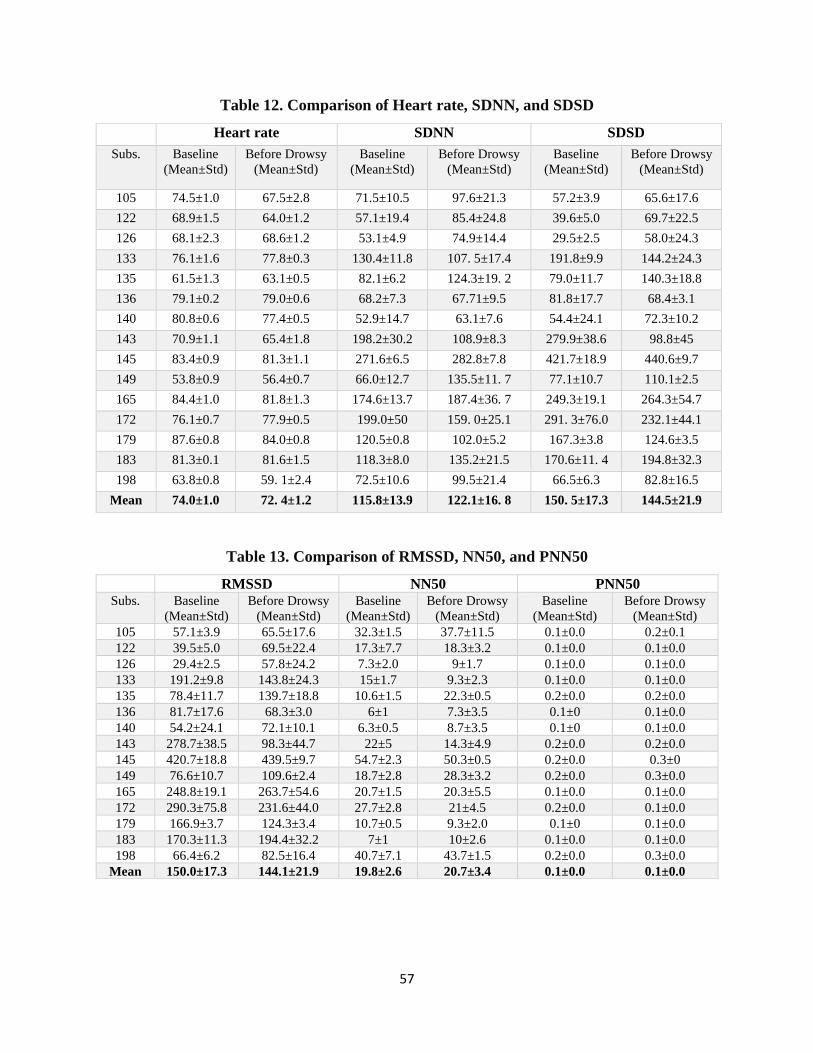
57

Table 12. Comparison of Heart rate, SDNN, and SDSD

Table 13. Comparison of RMSSD, NN50, and PNN50

Heart rate SDNN SDSD

Subs. Baseline

(Mean±Std)

Before Drowsy

(Mean±Std)

Baseline

(Mean±Std)

Before Drowsy

(Mean±Std)

Baseline

(Mean±Std)

Before Drowsy

(Mean±Std)

105 74.5±1.0 67.5±2.8 71.5±10.5 97.6±21.3 57.2±3.9 65.6±17.6

122 68.9±1.5 64.0±1.2 57.1±19.4 85.4±24.8 39.6±5.0 69.7±22.5

126 68.1±2.3 68.6±1.2 53.1±4.9 74.9±14.4 29.5±2.5 58.0±24.3

133 76.1±1.6 77.8±0.3 130.4±11.8 107. 5±17.4 191.8±9.9 144.2±24.3

135 61.5±1.3 63.1±0.5 82.1±6.2 124.3±19. 2 79.0±11.7 140.3±18.8

136 79.1±0.2 79.0±0.6 68.2±7.3 67.71±9.5 81.8±17.7 68.4±3.1

140 80.8±0.6 77.4±0.5 52.9±14.7 63.1±7.6 54.4±24.1 72.3±10.2

143 70.9±1.1 65.4±1.8 198.2±30.2 108.9±8.3 279.9±38.6 98.8±45

145 83.4±0.9 81.3±1.1 271.6±6.5 282.8±7.8 421.7±18.9 440.6±9.7

149 53.8±0.9 56.4±0.7 66.0±12.7 135.5±11. 7 77.1±10.7 110.1±2.5

165 84.4±1.0 81.8±1.3 174.6±13.7 187.4±36. 7 249.3±19.1 264.3±54.7

172 76.1±0.7 77.9±0.5 199.0±50 159. 0±25.1 291. 3±76.0 232.1±44.1

179 87.6±0.8 84.0±0.8 120.5±0.8 102.0±5.2 167.3±3.8 124.6±3.5

183 81.3±0.1 81.6±1.5 118.3±8.0 135.2±21.5 170.6±11. 4 194.8±32.3

198 63.8±0.8 59. 1±2.4 72.5±10.6 99.5±21.4 66.5±6.3 82.8±16.5

Mean 74.0±1.0 72. 4±1.2 115.8±13.9 122.1±16. 8 150. 5±17.3 144.5±21.9

RMSSD NN50 PNN50 Subs. Baseline

(Mean±Std)

Before Drowsy

(Mean±Std)

Baseline

(Mean±Std)

Before Drowsy

(Mean±Std)

Baseline

(Mean±Std)

Before Drowsy

(Mean±Std)

105 57.1±3.9 65.5±17.6 32.3±1.5 37.7±11.5 0.1±0.0 0.2±0.1

122 39.5±5.0 69.5±22.4 17.3±7.7 18.3±3.2 0.1±0.0 0.1±0.0

126 29.4±2.5 57.8±24.2 7.3±2.0 9±1.7 0.1±0.0 0.1±0.0

133 191.2±9.8 143.8±24.3 15±1.7 9.3±2.3 0.1±0.0 0.1±0.0

135 78.4±11.7 139.7±18.8 10.6±1.5 22.3±0.5 0.2±0.0 0.2±0.0

136 81.7±17.6 68.3±3.0 6±1 7.3±3.5 0.1±0 0.1±0.0

140 54.2±24.1 72.1±10.1 6.3±0.5 8.7±3.5 0.1±0 0.1±0.0

143 278.7±38.5 98.3±44.7 22±5 14.3±4.9 0.2±0.0 0.2±0.0

145 420.7±18.8 439.5±9.7 54.7±2.3 50.3±0.5 0.2±0.0 0.3±0

149 76.6±10.7 109.6±2.4 18.7±2.8 28.3±3.2 0.2±0.0 0.3±0.0

165 248.8±19.1 263.7±54.6 20.7±1.5 20.3±5.5 0.1±0.0 0.1±0.0

172 290.3±75.8 231.6±44.0 27.7±2.8 21±4.5 0.2±0.0 0.1±0.0

179 166.9±3.7 124.3±3.4 10.7±0.5 9.3±2.0 0.1±0 0.1±0.0

183 170.3±11.3 194.4±32.2 7±1 10±2.6 0.1±0.0 0.1±0.0

198 66.4±6.2 82.5±16.4 40.7±7.1 43.7±1.5 0.2±0.0 0.3±0.0

Mean 150.0±17.3 144.1±21.9 19.8±2.6 20.7±3.4 0.1±0.0 0.1±0.0

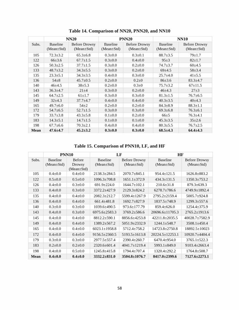
58

Table 14. Comparison of NN20, PNN20, and NN10

Table 15. Comparison of PNN10, LF, and HF

NN20 PNN20 NN10

Subs. Baseline

(Mean±Std)

Before Drowsy

(Mean±Std)

Baseline

(Mean±Std)

Before Drowsy

(Mean±Std)

Baseline

(Mean±Std)

Before Drowsy

(Mean±Std)

105 72.3±3.2 65.3±6.8 0.3±0.0 0.3±0.1 88.7±3.5 79±1.7

122 66±3.6 67.7±1.5 0.3±0.0 0.4±0.0 95±3 82±1.7

126 50.3±2.5 37.7±1.5 0.3±0.0 0.2±0.0 74.7±3.7 60±4.5

133 48.7±3.2 34.3±5.5 0.3±0.0 0.2±0.0 69±4.5 58±3.4

135 23.3±5.1 34.3±3.5 0.4±0.0 0.3±0.0 25.7±4.0 41±5.5

136 54±8 45.7±0.5 0.2±0.0 0.2±0 86±3.6 83.3±4.7

140 46±4.5 38±5.3 0.2±0.0 0.3±0 75.7±3.2 67±11.5

143 36.3±4.7 21±4 0.3±0.0 0.2±0.0 46±4.3 27±3

145 64.7±2.5 61±1.7 0.3±0.0 0.3±0.0 81.3±1.5 76.7±6.5

149 32±4.3 37.7±4.7 0.4±0.0 0.4±0.0 40.3±3.5 40±4.3

165 49.7±6.0 54±2 0.2±0.0 0.2±0.0 84.3±8.9 88.3±1.1

172 54.7±6.5 52.7±1.5 0.3±0.0 0.3±0.0 69.3±6.8 76.3±6.1

179 33.7±3.8 43.3±5.8 0.1±0.0 0.2±0.0 66±5 76.3±4.1

183 14.3±5.1 14.7±1.5 0.1±0.0 0.1±0.0 45.3±3.5 35±2.6

198 67.7±6.6 70.3±2.1 0.4±0.0 0.4±0.0 80.3±5.5 76.7±2.5

Mean 47.6±4.7 45.2±3.2 0.3±0.0 0.3±0.0 68.5±4.3 64.4±4.3

PNN10 LF HF

Subs. Baseline

(Mean±Std)

Before

Drowsy

(Mean±Std)

Baseline

(Mean±Std)

Before Drowsy

(Mean±Std)

Baseline

(Mean±Std)

Before Drowsy

(Mean±Std)

105 0.4±0.0 0.4±0.0 2138.3±284.5 2070.7±845.1 954.4±121.5 1626.8±883.2

122 0.5±0.0 0.5±0.0 1096.3±708.8 1651.1±372.9 434.3±131.5 1350.3±753.2

126 0.4±0.0 0.3±0.0 691.9±224.0 1644.7±102.1 210.6±31.8 879.3±639.3

133 0.4±0.0 0.3±0.0 3372.2±427.9 2129.3±824.2 6278.7±786.6 4749.9±1892.4

135 0.4±0.0 0.4±0.0 2082.3±212.7 5599.4±1267.9 2795.2±2159.4 5005.7±924.8

136 0.4±0.0 0.4±0.0 661.4±481.8 1692.7±827.9 1837.5±748.9 1299.3±557.6

140 0.3±0.0 0.3±0.0 1039.6±490.5 973.6±177.79 859.4±626.0 1254.4±375.9

143 0.4±0.0 0.3±0.0 6975.6±2583.3 3769.2±586.6 20696.6±11705.3 2765.2±1913.6

145 0.4±0.0 0.4±0.0 8812.2±590.1 8856.6±4253.8 42211.8±2035.5 40028.7±7582.9

149 0.4±0.0 0.4±0.0 1389.2±567.2 5051.9±2332.9 1244.1±548.7 3508.1±450.4

165 0.4±0.0 0.4±0.0 6023.1±1958.8 5712.4±758.2 14723.8±2750.8 18892.5±10023

172 0.4±0.0 0.4±0.0 9156.5±2360.5 5193.5±1613.8 20224.5±12253.1 10920.7±4404.4

179 0.3±0.0 0.3±0.0 2977.5±557.4 2390.4±260.7 6470.4±954.0 3765.1±522.3

183 0.2±0.0 0.2±0.0 2320.6±601.4 4041.7±1219.4 5993.1±849.0 9103.4±2663.4

198 0.4±0.0 0.5±0.0 1245.8±415.8 1794.4±707.4 1320.4±292.2 1764.8±508.7

Mean 0.4±0.0 0.4±0.0 3332.2±831.0 3504.8±1076.7 8417.0±2399.6 7127.6±2273.1

59

Table 16. LF(%), HF(%), and LF/HF values for baseline and before drowsy periods

3.1.3 Ultra-short HRV (30s)

Ultra-short HRV using 30s segmentations were tested to check the feasibility for faster

drowsiness detection. The same time domain and frequency domain parameters were extracted.

Two-Sample T-test has been used to identify the significant features, where most of the features

did not show significant change during drowsiness. The calculated p values for all the features

were: heart rate (p=0.13), SDNN (p=0.06), SDSD (p=0.08), RMSSD (p=0.08), NN50 (p=0.58),

pNN50 (p=0.16), LF percentage (p=0.14), HF percentage (p=0.14), LF(p<0.05)*, HF(p<0.05)*,

and LF/HF (p=0.17). Among all the features, LF and HF showed significant change during drowsy

periods compared to baseline periods. Tables 13 to 16 represent the time domain and frequency

domain feature values extracted for ultra-short HRV analysis.

LF (%) HF (%) LF /HF

Subs. Baseline

(Mean±Std)

Before Drowsy

(Mean±Std)

Baseline

(Mean±Std)

Before Drowsy

(Mean±Std)

Baseline

(Mean±Std)

Before

Drowsy

(Mean±Std)

105 69.1±0.9 57.0±3.3 30.8±0.9 42.9±3.3 2.2±0.1 1.3±0.2

122 68.5±11.0 57.7±10.8 31.5±11.0 42.2±10.8 2.4±1.0 1.5±0.7

126 75.8±5.5 68.2±19.6 24.2±5.5 31.7±19.6 3.2±1.1 3.9±4.3

133 34.9±3.2 31.0±0.2 65.0±3.2 68.9±0.2 0.5±0.1 0.4±0

135 47.7±18.5 52.5±4.0 52.2±18.5 47.4±4.0 1.0±0.6 1.2±0.2

136 24.7±6.0 55.0±10.3 75.2±6.0 44.9±10.3 0.3±0.1 1.3±0.6

140 59.8±13.6 44.1±6.8 40.1±13.6 55.8±6.8 1.7±1.1 0.8±0.2

143 26.7±5.0 60.3±16.1 73.3±5.0 39.7±16.0 0.3±0.1 1.8±1.1

145 17.3±1.5 18.5±9.5 82.7±1.5 81.5±9.5 0.2±0.0 0.2±0.1

149 52.9±4.2 56.6±12.3 47.0±4.2 43.3±12.3 1.1±0.1 1.4±0.6

165 28.7±4.7 25.9±9.6 71.3±4.7 74.1±9.6 0.4±0.1 0.3±0.2

172 34.9±12.1 32.7±3.0 65.0±12.1 67.2±3.0 0.5±0.3 0.4±0.1

179 31.5±2.6 39±5.6 68.5±2.5 61±5.6 0.4±0.0 0.6±0.1

183 27.6±3.8 30.6±0.3 72.3±3.7 69.3±0.3 0.3±0.0 0.4±0.0

198 48.1±13.9 49.8±3.4 51.9±13.9 50.1±3.4 1.02±0.5 1±0.1

Mean 43.2±7.1 45.3±7.7 56.7±7.1 54.7±7.7 1.0±0.3 1.1±0.6

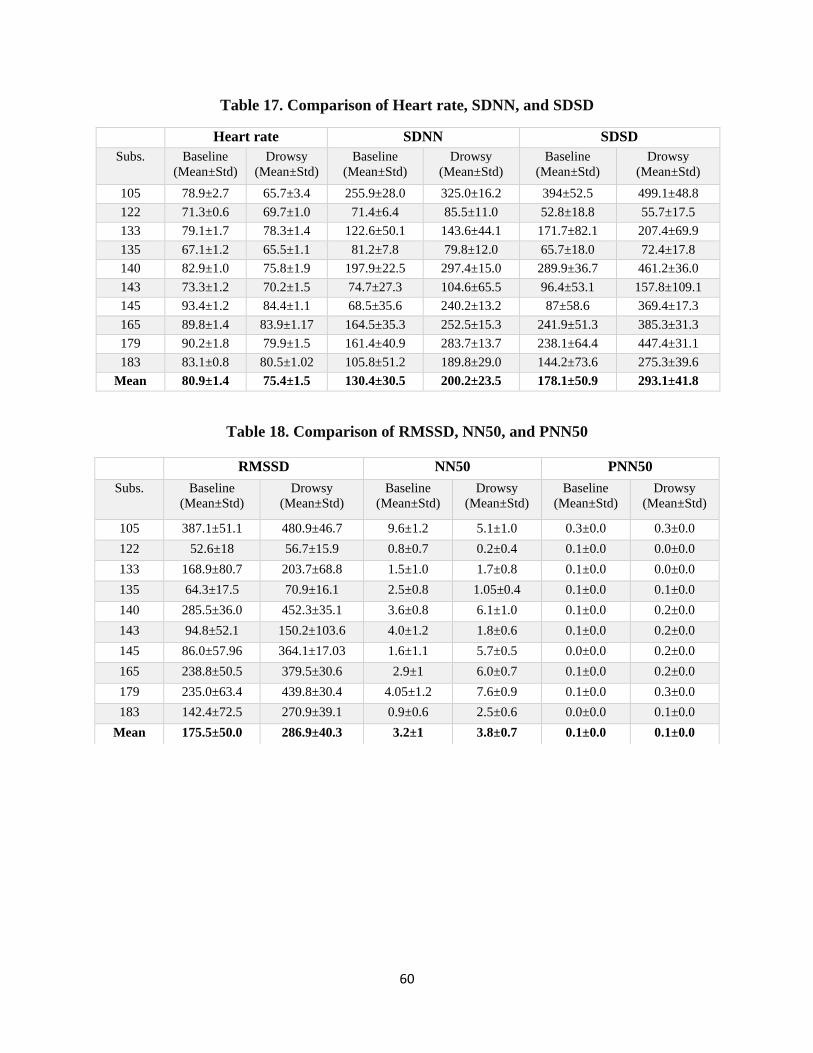
60

Table 17. Comparison of Heart rate, SDNN, and SDSD

Heart rate SDNN SDSD

Subs. Baseline

(Mean±Std)

Drowsy

(Mean±Std)

Baseline

(Mean±Std)

Drowsy

(Mean±Std)

Baseline

(Mean±Std)

Drowsy

(Mean±Std)

105 78.9±2.7 65.7±3.4 255.9±28.0 325.0±16.2 394±52.5 499.1±48.8

122 71.3±0.6 69.7±1.0 71.4±6.4 85.5±11.0 52.8±18.8 55.7±17.5

133 79.1±1.7 78.3±1.4 122.6±50.1 143.6±44.1 171.7±82.1 207.4±69.9

135 67.1±1.2 65.5±1.1 81.2±7.8 79.8±12.0 65.7±18.0 72.4±17.8

140 82.9±1.0 75.8±1.9 197.9±22.5 297.4±15.0 289.9±36.7 461.2±36.0

143 73.3±1.2 70.2±1.5 74.7±27.3 104.6±65.5 96.4±53.1 157.8±109.1

145 93.4±1.2 84.4±1.1 68.5±35.6 240.2±13.2 87±58.6 369.4±17.3

165 89.8±1.4 83.9±1.17 164.5±35.3 252.5±15.3 241.9±51.3 385.3±31.3

179 90.2±1.8 79.9±1.5 161.4±40.9 283.7±13.7 238.1±64.4 447.4±31.1

183 83.1±0.8 80.5±1.02 105.8±51.2 189.8±29.0 144.2±73.6 275.3±39.6

Mean 80.9±1.4 75.4±1.5 130.4±30.5 200.2±23.5 178.1±50.9 293.1±41.8

Table 18. Comparison of RMSSD, NN50, and PNN50

RMSSD NN50 PNN50

Subs. Baseline

(Mean±Std)

Drowsy

(Mean±Std)

Baseline

(Mean±Std)

Drowsy

(Mean±Std)

Baseline

(Mean±Std)

Drowsy

(Mean±Std)

105 387.1±51.1 480.9±46.7 9.6±1.2 5.1±1.0 0.3±0.0 0.3±0.0

122 52.6±18 56.7±15.9 0.8±0.7 0.2±0.4 0.1±0.0 0.0±0.0

133 168.9±80.7 203.7±68.8 1.5±1.0 1.7±0.8 0.1±0.0 0.0±0.0

135 64.3±17.5 70.9±16.1 2.5±0.8 1.05±0.4 0.1±0.0 0.1±0.0

140 285.5±36.0 452.3±35.1 3.6±0.8 6.1±1.0 0.1±0.0 0.2±0.0

143 94.8±52.1 150.2±103.6 4.0±1.2 1.8±0.6 0.1±0.0 0.2±0.0

145 86.0±57.96 364.1±17.03 1.6±1.1 5.7±0.5 0.0±0.0 0.2±0.0

165 238.8±50.5 379.5±30.6 2.9±1 6.0±0.7 0.1±0.0 0.2±0.0

179 235.0±63.4 439.8±30.4 4.05±1.2 7.6±0.9 0.1±0.0 0.3±0.0

183 142.4±72.5 270.9±39.1 0.9±0.6 2.5±0.6 0.0±0.0 0.1±0.0

Mean 175.5±50.0 286.9±40.3 3.2±1 3.8±0.7 0.1±0.0 0.1±0.0

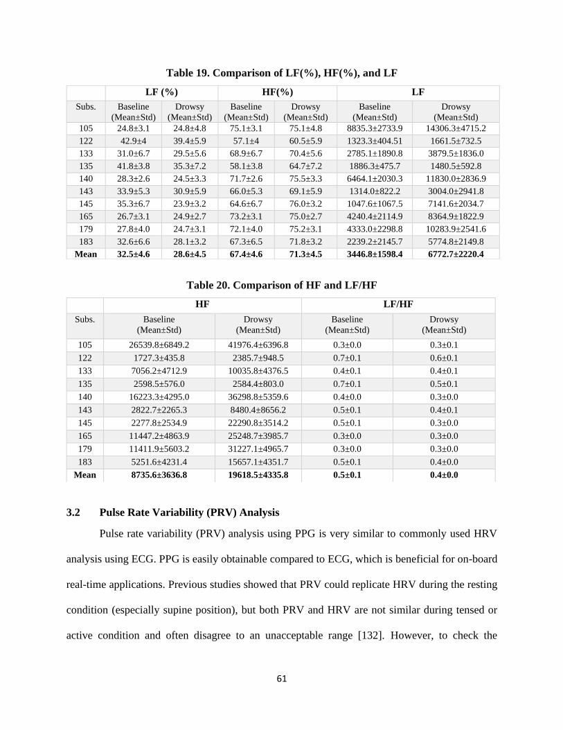
61

Table 19. Comparison of LF(%), HF(%), and LF

Table 20. Comparison of HF and LF/HF

3.2 Pulse Rate Variability (PRV) Analysis

Pulse rate variability (PRV) analysis using PPG is very similar to commonly used HRV

analysis using ECG. PPG is easily obtainable compared to ECG, which is beneficial for on-board

real-time applications. Previous studies showed that PRV could replicate HRV during the resting

condition (especially supine position), but both PRV and HRV are not similar during tensed or

active condition and often disagree to an unacceptable range [132]. However, to check the

LF (%) HF(%) LF

Subs. Baseline

(Mean±Std)

Drowsy

(Mean±Std)

Baseline

(Mean±Std)

Drowsy

(Mean±Std)

Baseline

(Mean±Std)

Drowsy

(Mean±Std)

105 24.8±3.1 24.8±4.8 75.1±3.1 75.1±4.8 8835.3±2733.9 14306.3±4715.2

122 42.9±4 39.4±5.9 57.1±4 60.5±5.9 1323.3±404.51 1661.5±732.5

133 31.0±6.7 29.5±5.6 68.9±6.7 70.4±5.6 2785.1±1890.8 3879.5±1836.0

135 41.8±3.8 35.3±7.2 58.1±3.8 64.7±7.2 1886.3±475.7 1480.5±592.8

140 28.3±2.6 24.5±3.3 71.7±2.6 75.5±3.3 6464.1±2030.3 11830.0±2836.9

143 33.9±5.3 30.9±5.9 66.0±5.3 69.1±5.9 1314.0±822.2 3004.0±2941.8

145 35.3±6.7 23.9±3.2 64.6±6.7 76.0±3.2 1047.6±1067.5 7141.6±2034.7

165 26.7±3.1 24.9±2.7 73.2±3.1 75.0±2.7 4240.4±2114.9 8364.9±1822.9

179 27.8±4.0 24.7±3.1 72.1±4.0 75.2±3.1 4333.0±2298.8 10283.9±2541.6

183 32.6±6.6 28.1±3.2 67.3±6.5 71.8±3.2 2239.2±2145.7 5774.8±2149.8

Mean 32.5±4.6 28.6±4.5 67.4±4.6 71.3±4.5 3446.8±1598.4 6772.7±2220.4

HF LF/HF

Subs. Baseline

(Mean±Std)

Drowsy

(Mean±Std)

Baseline

(Mean±Std)

Drowsy

(Mean±Std)

105 26539.8±6849.2 41976.4±6396.8 0.3±0.0 0.3±0.1

122 1727.3±435.8 2385.7±948.5 0.7±0.1 0.6±0.1

133 7056.2±4712.9 10035.8±4376.5 0.4±0.1 0.4±0.1

135 2598.5±576.0 2584.4±803.0 0.7±0.1 0.5±0.1

140 16223.3±4295.0 36298.8±5359.6 0.4±0.0 0.3±0.0

143 2822.7±2265.3 8480.4±8656.2 0.5±0.1 0.4±0.1

145 2277.8±2534.9 22290.8±3514.2 0.5±0.1 0.3±0.0

165 11447.2±4863.9 25248.7±3985.7 0.3±0.0 0.3±0.0

179 11411.9±5603.2 31227.1±4965.7 0.3±0.0 0.3±0.0

183 5251.6±4231.4 15657.1±4351.7 0.5±0.1 0.4±0.0

Mean 8735.6±3636.8 19618.5±4335.8 0.5±0.1 0.4±0.0

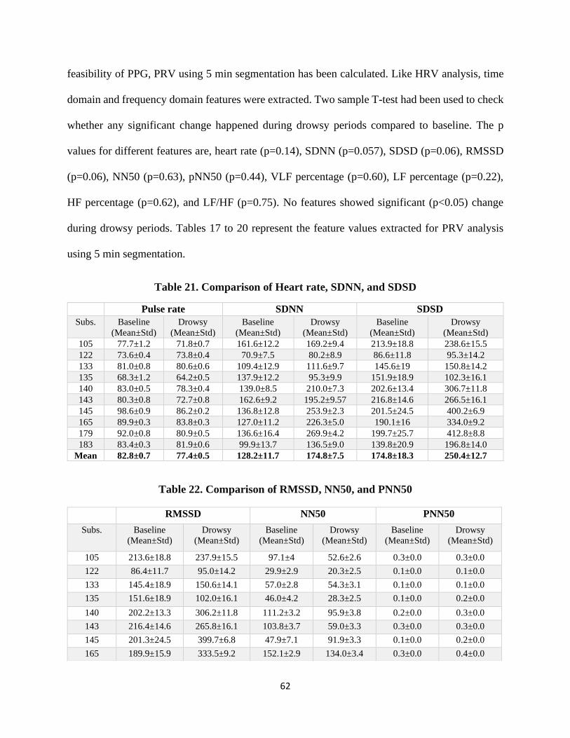
62

feasibility of PPG, PRV using 5 min segmentation has been calculated. Like HRV analysis, time

domain and frequency domain features were extracted. Two sample T-test had been used to check

whether any significant change happened during drowsy periods compared to baseline. The p

values for different features are, heart rate (p=0.14), SDNN (p=0.057), SDSD (p=0.06), RMSSD

(p=0.06), NN50 (p=0.63), pNN50 (p=0.44), VLF percentage (p=0.60), LF percentage (p=0.22),

HF percentage (p=0.62), and LF/HF (p=0.75). No features showed significant (p<0.05) change

during drowsy periods. Tables 17 to 20 represent the feature values extracted for PRV analysis

using 5 min segmentation.

Table 21. Comparison of Heart rate, SDNN, and SDSD

Pulse rate SDNN SDSD

Subs. Baseline

(Mean±Std)

Drowsy

(Mean±Std)

Baseline

(Mean±Std)

Drowsy

(Mean±Std)

Baseline

(Mean±Std)

Drowsy

(Mean±Std)

105 77.7±1.2 71.8±0.7 161.6±12.2 169.2±9.4 213.9±18.8 238.6±15.5

122 73.6±0.4 73.8±0.4 70.9±7.5 80.2±8.9 86.6±11.8 95.3±14.2

133 81.0±0.8 80.6±0.6 109.4±12.9 111.6±9.7 145.6±19 150.8±14.2

135 68.3±1.2 64.2±0.5 137.9±12.2 95.3±9.9 151.9±18.9 102.3±16.1

140 83.0±0.5 78.3±0.4 139.0±8.5 210.0±7.3 202.6±13.4 306.7±11.8

143 80.3±0.8 72.7±0.8 162.6±9.2 195.2±9.57 216.8±14.6 266.5±16.1

145 98.6±0.9 86.2±0.2 136.8±12.8 253.9±2.3 201.5±24.5 400.2±6.9

165 89.9±0.3 83.8±0.3 127.0±11.2 226.3±5.0 190.1±16 334.0±9.2

179 92.0±0.8 80.9±0.5 136.6±16.4 269.9±4.2 199.7±25.7 412.8±8.8

183 83.4±0.3 81.9±0.6 99.9±13.7 136.5±9.0 139.8±20.9 196.8±14.0

Mean 82.8±0.7 77.4±0.5 128.2±11.7 174.8±7.5 174.8±18.3 250.4±12.7

Table 22. Comparison of RMSSD, NN50, and PNN50

RMSSD NN50 PNN50

Subs. Baseline

(Mean±Std)

Drowsy

(Mean±Std)

Baseline

(Mean±Std)

Drowsy

(Mean±Std)

Baseline

(Mean±Std)

Drowsy

(Mean±Std)

105 213.6±18.8 237.9±15.5 97.1±4 52.6±2.6 0.3±0.0 0.3±0.0

122 86.4±11.7 95.0±14.2 29.9±2.9 20.3±2.5 0.1±0.0 0.1±0.0

133 145.4±18.9 150.6±14.1 57.0±2.8 54.3±3.1 0.1±0.0 0.1±0.0

135 151.6±18.9 102.0±16.1 46.0±4.2 28.3±2.5 0.1±0.0 0.2±0.0

140 202.2±13.3 306.2±11.8 111.2±3.2 95.9±3.8 0.2±0.0 0.3±0.0

143 216.4±14.6 265.8±16.1 103.8±3.7 59.0±3.3 0.3±0.0 0.3±0.0

145 201.3±24.5 399.7±6.8 47.9±7.1 91.9±3.3 0.1±0.0 0.2±0.0

165 189.9±15.9 333.5±9.2 152.1±2.9 134.0±3.4 0.3±0.0 0.4±0.0

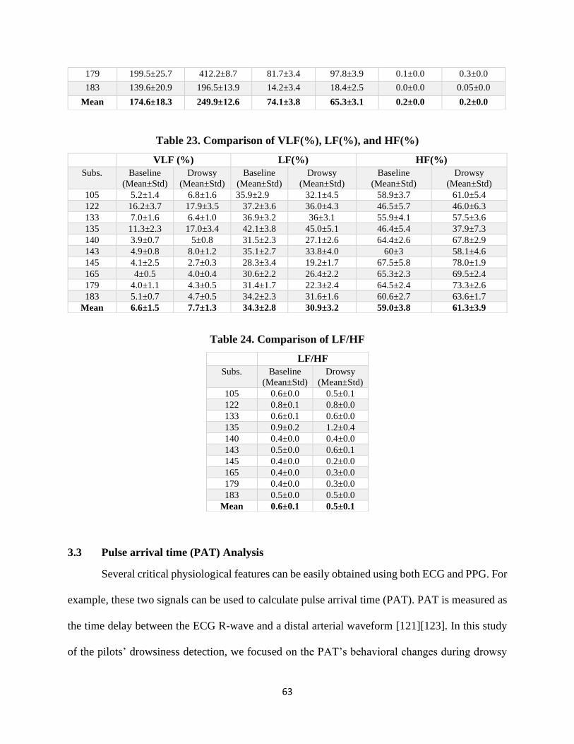
63

Table 23. Comparison of VLF(%), LF(%), and HF(%)

Table 24. Comparison of LF/HF

3.3 Pulse arrival time (PAT) Analysis

Several critical physiological features can be easily obtained using both ECG and PPG. For

example, these two signals can be used to calculate pulse arrival time (PAT). PAT is measured as

the time delay between the ECG R-wave and a distal arterial waveform [121][123]. In this study

of the pilots’ drowsiness detection, we focused on the PAT’s behavioral changes during drowsy

179 199.5±25.7 412.2±8.7 81.7±3.4 97.8±3.9 0.1±0.0 0.3±0.0

183 139.6±20.9 196.5±13.9 14.2±3.4 18.4±2.5 0.0±0.0 0.05±0.0

Mean 174.6±18.3 249.9±12.6 74.1±3.8 65.3±3.1 0.2±0.0 0.2±0.0

VLF (%) LF(%) HF(%)

Subs. Baseline

(Mean±Std)

Drowsy

(Mean±Std)

Baseline

(Mean±Std)

Drowsy

(Mean±Std)

Baseline

(Mean±Std)

Drowsy

(Mean±Std)

105 5.2±1.4 6.8±1.6 35.9±2.9 32.1±4.5 58.9±3.7 61.0±5.4

122 16.2±3.7 17.9±3.5 37.2±3.6 36.0±4.3 46.5±5.7 46.0±6.3

133 7.0±1.6 6.4±1.0 36.9±3.2 36±3.1 55.9±4.1 57.5±3.6

135 11.3±2.3 17.0±3.4 42.1±3.8 45.0±5.1 46.4±5.4 37.9±7.3

140 3.9±0.7 5±0.8 31.5±2.3 27.1±2.6 64.4±2.6 67.8±2.9

143 4.9±0.8 8.0±1.2 35.1±2.7 33.8±4.0 60±3 58.1±4.6

145 4.1±2.5 2.7±0.3 28.3±3.4 19.2±1.7 67.5±5.8 78.0±1.9

165 4±0.5 4.0±0.4 30.6±2.2 26.4±2.2 65.3±2.3 69.5±2.4

179 4.0±1.1 4.3±0.5 31.4±1.7 22.3±2.4 64.5±2.4 73.3±2.6

183 5.1±0.7 4.7±0.5 34.2±2.3 31.6±1.6 60.6±2.7 63.6±1.7

Mean 6.6±1.5 7.7±1.3 34.3±2.8 30.9±3.2 59.0±3.8 61.3±3.9

LF/HF

Subs. Baseline

(Mean±Std)

Drowsy

(Mean±Std)

105 0.6±0.0 0.5±0.1

122 0.8±0.1 0.8±0.0

133 0.6±0.1 0.6±0.0

135 0.9±0.2 1.2±0.4

140 0.4±0.0 0.4±0.0

143 0.5±0.0 0.6±0.1

145 0.4±0.0 0.2±0.0

165 0.4±0.0 0.3±0.0

179 0.4±0.0 0.3±0.0

183 0.5±0.0 0.5±0.0

Mean 0.6±0.1 0.5±0.1

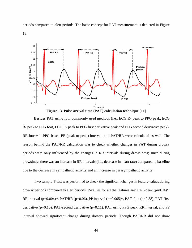
64

periods compared to alert periods. The basic concept for PAT measurement is depicted in Figure

13.

Figure 13. Pulse arrival time (PAT) calculation technique [11]

Besides PAT using four commonly used methods (i.e., ECG R- peak to PPG peak, ECG

R- peak to PPG foot, ECG R- peak to PPG first derivative peak and PPG second derivative peak),

RR interval, PPG based PP (peak to peak) interval, and PAT/RR were calculated as well. The

reason behind the PAT/RR calculation was to check whether changes in PAT during drowsy

periods were only influenced by the changes in RR intervals during drowsiness; since during

drowsiness there was an increase in RR intervals (i.e., decrease in heart rate) compared to baseline

due to the decrease in sympathetic activity and an increase in parasympathetic activity.

Two sample T-test was performed to check the significant changes in feature values during

drowsy periods compared to alert periods. P-values for all the features are: PAT-peak (p=0.04)*,

RR interval (p=0.004)*, PAT/RR (p=0.06), PP interval (p=0.005)*, PAT-foot (p=0.88), PAT-first

derivative (p=0.10), PAT-second derivative (p=0.11). PAT using PPG peak, RR interval, and PP

interval showed significant change during drowsy periods. Though PAT/RR did not show

Vo

ltag

e (m

V)

Time (s)

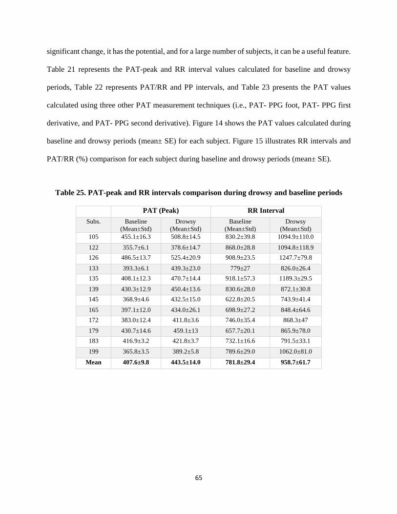
65

significant change, it has the potential, and for a large number of subjects, it can be a useful feature.

Table 21 represents the PAT-peak and RR interval values calculated for baseline and drowsy

periods, Table 22 represents PAT/RR and PP intervals, and Table 23 presents the PAT values

calculated using three other PAT measurement techniques (i.e., PAT- PPG foot, PAT- PPG first

derivative, and PAT- PPG second derivative). Figure 14 shows the PAT values calculated during

baseline and drowsy periods (mean± SE) for each subject. Figure 15 illustrates RR intervals and

PAT/RR (%) comparison for each subject during baseline and drowsy periods (mean± SE).

Table 25. PAT-peak and RR intervals comparison during drowsy and baseline periods

PAT (Peak) RR Interval

Subs. Baseline

(Mean±Std)

Drowsy

(Mean±Std)

Baseline

(Mean±Std)

Drowsy

(Mean±Std)

105 455.1±16.3 508.8±14.5 830.2±39.8 1094.9±110.0

122 355.7±6.1 378.6±14.7 868.0±28.8 1094.8±118.9

126 486.5±13.7 525.4±20.9 908.9±23.5 1247.7±79.8

133 393.3±6.1 439.3±23.0 779±27 826.0±26.4

135 408.1±12.3 470.7±14.4 918.1±57.3 1189.3±29.5

139 430.3±12.9 450.4±13.6 830.6±28.0 872.1±30.8

145 368.9±4.6 432.5±15.0 622.8±20.5 743.9±41.4

165 397.1±12.0 434.0±26.1 698.9±27.2 848.4±64.6

172 383.0±12.4 411.8±3.6 746.0±35.4 868.3±47

179 430.7±14.6 459.1±13 657.7±20.1 865.9±78.0

183 416.9±3.2 421.8±3.7 732.1±16.6 791.5±33.1

199 365.8±3.5 389.2±5.8 789.6±29.0 1062.0±81.0

Mean 407.6±9.8 443.5±14.0 781.8±29.4 958.7±61.7

66

Figure 14. Pulse arrival time (PAT) comparison during baseline and drowsy periods (mean±

SE). (Black and red color indicate during the baseline and drowsy periods respectively) [11]

Figure 15. RR interval and PAT/RR (%) comparison for each subject during baseline and

drowsy periods. (Black and red color indicate during the baseline and drowsy periods

respectively) [11]

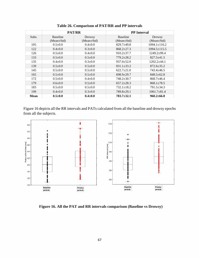
67

Table 26. Comparison of PAT/RR and PP intervals

Figure 16 depicts all the RR intervals and PATs calculated from all the baseline and drowsy epochs

from all the subjects.

PAT/RR PP Interval

Subs. Baseline

(Mean±Std)

Drowsy

(Mean±Std)

Baseline

(Mean±Std)

Drowsy

(Mean±Std)

105 0.5±0.0 0.4±0.0 829.7±49.8 1094.1±116.2

122 0.4±0.0 0.3±0.0 868.2±27.3 1094.5±115.5

126 0.5±0.0 0.4±0.0 910.2±37.7 1249.2±99.4

133 0.5±0.0 0.5±0.0 779.2±28.2 827.5±41.5

135 0.4±0.0 0.3±0.0 937.0±52.0 1202.2±44.1

139 0.5±0.0 0.5±0.0 831.1±33.2 872.6±35.2

145 0.5±0.0 0.5±0.0 622.7±21.0 743.4±46.5

165 0.5±0.0 0.5±0.0 698.9±29.7 848.5±62.8

172 0.5±0.0 0.4±0.0 748.2±30.7 868.7±46.4

179 0.6±0.0 0.5±0.0 657.2±28.3 868.1±78.5

183 0.5±0.0 0.5±0.0 732.1±18.2 791.5±34.3

199 0.4±0.0 0.3±0.0 789.8±29.1 1061.7±81.4

Mean 0.5±0.0 0.4±0.0 783.7±32.1 960.2±66.8

Figure 16. All the PAT and RR intervals comparison (Baseline vs Drowsy)

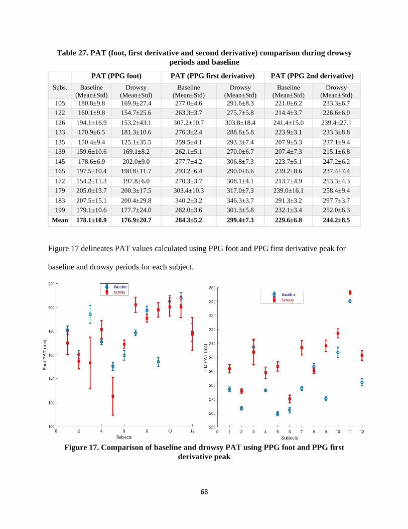
68

Table 27. PAT (foot, first derivative and second derivative) comparison during drowsy

periods and baseline

Figure 17 delineates PAT values calculated using PPG foot and PPG first derivative peak for

baseline and drowsy periods for each subject.

Figure 17. Comparison of baseline and drowsy PAT using PPG foot and PPG first

derivative peak

PAT (PPG foot) PAT (PPG first derivative) PAT (PPG 2nd derivative)

Subs. Baseline

(Mean±Std)

Drowsy

(Mean±Std)

Baseline

(Mean±Std)

Drowsy

(Mean±Std)

Baseline

(Mean±Std)

Drowsy

(Mean±Std)

105 180.8±9.8 169.9±27.4 277.0±4.6 291.6±8.3 221.0±6.2 233.3±6.7

122 160.1±9.8 154.7±25.6 263.3±3.7 275.7±5.8 214.4±3.7 226.6±6.0

126 194.1±16.9 153.2±43.1 307.2±10.7 303.8±18.4 241.4±15.0 239.4±27.1

133 170.9±6.5 181.3±10.6 276.3±2.4 288.8±5.8 223.9±3.1 233.3±8.8

135 150.4±9.4 125.1±35.5 259.5±4.1 293.3±7.4 207.9±5.3 237.1±9.4

139 159.6±10.6 169.1±8.2 262.1±5.1 270.0±6.7 207.4±7.3 215.1±6.8

145 178.6±6.9 202.0±9.0 277.7±4.2 306.8±7.3 223.7±5.1 247.2±6.2

165 197.5±10.4 190.8±11.7 293.2±6.4 290.0±6.6 239.2±8.6 237.4±7.4

172 154.2±11.3 197.8±6.0 270.3±3.7 308.1±4.1 213.7±4.9 253.3±4.3

179 205.0±13.7 200.3±17.5 303.4±10.3 317.0±7.3 239.0±16.1 258.4±9.4

183 207.5±15.1 200.4±29.8 340.2±3.2 346.3±3.7 291.3±3.2 297.7±3.7

199 179.1±10.6 177.7±24.0 282.0±3.6 301.3±5.8 232.1±3.4 252.0±6.3

Mean 178.1±10.9 176.9±20.7 284.3±5.2 299.4±7.3 229.6±6.8 244.2±8.5

69

Figure 18 illustrates the comparison of baseline and drowsy PATs using PPG second derivative

peaks.

Figure 18. Comparison of baseline and drowsy PAT using PPG second derivative peak

3.4 PPG Waveform based Features Extraction

3.4.1 Commonly used PPG features

Besides PAT, some other only PPG based features feasibility were checked for drowsiness

detection, namely: systolic amplitude (i.e., PPG foot to PPG peak height), crest time (time required

to reach PPG peak from the previous PPG foot), pulse interval (PPG foot to foot distance), ratio

of pulse interval and systolic amplitude, and diastolic time (time required to reach the next foot

from the current PPG peak). Figure 19 illustrates all the features just mentioned. Two sample T-

test showed three features that have the potential (p<0.05) to discriminate drowsy and baseline

70

periods, which are crest time (p=0.047) *, pulse interval (p=0.007) *, and diastolic time (p=0.009)

*. Two other features did not show any significant changes, systolic amplitude (p=0.55) and pulse

interval/systolic amplitude (p=0.239).

Figure 19. PPG waveform based features extraction [11]

Tables 24 and 25 represent the comparison of the feature values calculated during baseline and

drowsy periods.

Table 28. PPG based features (systolic amplitude, crest time, and pulse interval)

comparison during baseline and drowsy periods

Systolic Amplitude Crest Time Pulse Interval

Subs. Baseline

(Mean±Std)

Drowsy

(Mean±Std)

Baseline

(Mean±Std)

Drowsy

(Mean±Std)

Baseline

(Mean±Std)

Drowsy

(Mean±Std)

105 0.8±0.0 0.8±0.1 270.4±20.0 346.9±43.9 813.4±42.6 1093.7±110.3

122 0.7±0.0 0.8±0.1 194.6±11.3 249.9±51.9 854.8±31.0 1094.8±125.1

126 0.6±0.1 0.2±0.0 287.9±15.9 404.2±63.2 925.4±29.3 1248.9±110.0

133 1.7±0.1 0.9±0.0 222.3±9.9 242.6±25.0 778.9±27.1 805.1±35.4

135 1.2±0.1 1.3±0.2 252.6±20.0 343.4±45.6 946.7±67.9 1202.0±65.3

139 1.1±0.1 1.1±0.1 270.6±16.0 281.3±15.4 830.3±33.0 872.1±33.6

145 2.1±0.1 1.2±0.1 192.7±10.4 230.5±16.2 633.9±34.2 743.7±43.2

165 0.3±0.0 0.4±0.0 200.5±18.2 243.8±31.2 702.7±37.1 849±65.3

172 0.8±0.0 0.6±0.0 232.4±14.2 213.6±6.1 771.9±33.3 868.9±47.5

179 0.6±0.1 1.0±0.1 231.7±24.2 259±23.3 672.1±36.5 867.2±81.1

183 4.7±0.2 3.5±0.3 209.4±15.2 231.2±34.9 732.6±19.7 791.3±40.9

199 1.2±0.2 1.3±0.3 196.1±14.9 214.4±30.5 810.0±49.9 1058.2±81.1

Mean 1.3±0.1 1.1±0.1 230.1±15.9 271.7±32.3 789.4±36.8 957.9±69.9

71

Table 29. PPG based features (pulse interval/systolic amplitude and diastolic time)

comparison during drowsy periods and baseline

Figure 20 illustrates the comparison of crest time and diastolic time during baseline and drowsy

periods (mean ± SE).

Figure 20. Increase in PPG crest time and diastolic time (Mean ± standard error (SE)) during

drowsy periods compared to alert periods [11]

Pulse Interval/Systolic Amplitude Diastolic Time Subs. Baseline

(Mean±Std)

Drowsy

(Mean±Std)

Baseline

(Mean±Std)

Drowsy

(Mean±Std)

105 954.7±78.2 1347.0±153.4 543.5±37.6 747.0±90.0

122 1137.4±109.9 1330.3±150.1 660.2±25.9 844.3±91.5

126 1427.5±233.5 4782.6±486.2 636.5±23.7 844.1±76.0

133 445.2±34.2 887.5±102.7 556.5±24 566.0±31.3

135 769.5±82.2 1023.7±157.7 693.4±54.0 858.6±44.6

139 700.9±58.6 775.6±79.7 560.3±28.9 590.8±30.4

145 295.1±18.6 671.4±86.5 441.5±26.9 512.9±36.9

165 2084.5±260.3 2024.1±319.8 501.9±30.0 605.1±51.1

172 947.2±51.5 1279.5±105.1 540.4±23.2 655.1±43.3

179 1061.8±173.1 826.1±79.8 441.4±23.7 607.9±66.8

183 158.7±9.9 233.0±31.8 522.9±9.0 559.9±15.9

199 642.3±111.7 825.4±155.0 614.9±40.2 846.4±74.2

Mean 885.4±101.8 1333.9±159.0 559.4±28.9 686.5±54.3

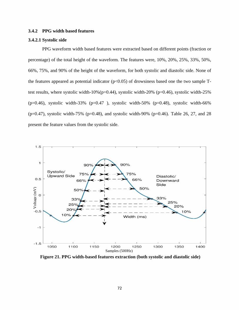
72

3.4.2 PPG width based features

3.4.2.1 Systolic side

PPG waveform width based features were extracted based on different points (fraction or

percentage) of the total height of the waveform. The features were, 10%, 20%, 25%, 33%, 50%,

66%, 75%, and 90% of the height of the waveform, for both systolic and diastolic side. None of

the features appeared as potential indicator (p<0.05) of drowsiness based one the two sample T-

test results, where systolic width-10%(p=0.44), systolic width-20% (p=0.46), systolic width-25%

(p=0.46), systolic width-33% (p=0.47 ), systolic width-50% (p=0.48), systolic width-66%

(p=0.47), systolic width-75% (p=0.48), and systolic width-90% (p=0.46). Table 26, 27, and 28

present the feature values from the systolic side.

Figure 21. PPG width-based features extraction (both systolic and diastolic side)

Samples (500Hz)

Vo

ltag

e (m

V)

73

Table 30. PPG width based features (10%, 20%, and 25% of the systolic peak) comparison

(systolic side)

Table 31. PPG width based features (33%, 50%, and 66% of the systolic peak) comparison

(systolic side)

Systolic Width (10%) Systolic Width (20%) Systolic Width (25%)

Subs. Baseline

(Mean±Std)

Drowsy

(Mean±Std)

Baseline

(Mean±Std)

Drowsy

(Mean±Std)

Baseline

(Mean±Std)

Drowsy

(Mean±Std)

105 235.2±31.3 269.4±20.5 216.0±29.5 246.8±19.7 208.0±28.3 237.6±19.4

122 144.7±7.4 157.8±14.1 126.4±6.8 139.0±13.6 119.4±6.6 131.9±13.4

126 266.5±65.6 321.5±50.7 243.1±62.2 294.2±48.5 233.6±61.1 283.4±48.2

133 172.1±9.8 203.9±21 154.3±9.6 184.8±21.7 147.0±9.5 177.4±21.8

135 187.5±26.6 192.5±30.1 167.3±25.9 171.3±28.4 159.8±25.6 163.5±27.7

139 226.4±12.7 226.1±14.3 207.3±12.6 207.1±13.9 199.3±12.5 199.3±13.9

145 157.3±15.7 175.8±13.4 139.4±14.8 157.3±12.8 132.1±14.4 149.7±12.6

165 184.4±34.3 197.4±28.0 167.3±33.7 179.9±27.4 160.3±33.3 172.8±27.2

172 166.0±9.5 159.0±4.7 147.0±8.8 140.6±4.1 139.5±8.4 133.4±4

179 189.4±18.1 199.5±15.8 170.4±17.3 179.5±15.2 162.3±16.7 171.1±14.9

183 137.6±2.8 137.0±3.2 118.0±2.2 117.5±2.3 110.4±1.9 110.1±2.1

199 140.5±8.5 146.4±7.4 123.0±7.2 127.8±6.6 115.9±6.7 120.5±6.2

Mean 184.0±20.2 198.9±18.6 165±19.2 178.8±17.8 157.3±18.8 170.9±17.6

Systolic Width (33%) Systolic Width (50%) Systolic Width (66%)

Subs. Baseline

(Mean±Std)

Drowsy

(Mean±Std)

Baseline

(Mean±Std)

Drowsy

(Mean±Std)

Baseline

(Mean±Std)

Drowsy

(Mean±Std)

105 195.8±26.8 223.7±19.3 171.2±23.3 194.7±19.1 143.4±18.8 161.2±19.5

122 109.3±6.6 121.7±13.3 90.4±6.2 102.3±12.9 73.0±5.9 84.5±12.4

126 219.8±59.6 266.8±47.8 191.2±54.9 231.8±46.6 155.8±34.6 189.4±38.5

133 136.7±9.3 166.4±22.1 116.8±9.2 144.7±22.2 97.8±8.9 123.7±22.0

135 148.6±25.2 151.8±26.9 127.9±24.2 130.2±24.8 108.1±22.5 109.6±22.4

139 187.7±12.7 187.8±13.7 164.3±12.7 164.4±13.1 139.6±13.0 139.5±12.6

145 121.9±13.7 138.8±12.1 101.8±12.6 117.3±11.1 82.7±10.9 96.6±9.8

165 150.3±33.1 162.4±26.8 130.6±32.0 142.1±25.7 111.6±30.7 122.2±24.3

172 128.5±8.15 122.6±3.8 107.7±7.5 102.5±3.5 88.1±6.8 83.6±3.2

179 150.9±16.5 159.5±14.7 128.2±15.8 136.6±14.2 105.6±14.7 114.07±13.3

183 100.0±1.9 99.6±1.9 80.8±1.5 80.6±1.7 63.6±1.5 63.7±1.5

199 106.3±6.4 110.5±6 87.7±5.6 91.2±5.2 70.7±5.04 73.8±4.8

Mean 146.3±18.3 159.3±17.3 124.9±17.1 136.5±16.7 103.3±14.4 113.5±15.3

74

Table 32. PPG width based features (75% and 90% of the systolic peak) comparison

(systolic side)

3.4.2.2 Diastolic side

For the diastolic side of the PPG waveform, the T-test result is quite same. None of the

features from diastolic side appeared as potential indicator (p<0.05) of drowsiness. Two sample

T-test results: diastolic width-10%(p=0.19), diastolic width-20%(p=0.22), diastolic width-

25%(p=0.30), diastolic width-33%(p=0.41), diastolic width-50%(p=0.44), diastolic width-

66%(p=0.51), diastolic width-75%(p=0.55), and diastolic width-90%(p=0.65). Table 29, 30, and

31 represent the feature values for both baseline and drowsy periods calculated from the PPG

diastolic side.

Table 33. PPG width based features (10%, 20%, and 25% of the systolic peak)

comparison (diastolic side)

Systolic Width (75%) Systolic Width (90%)

Subs. Baseline

(Mean±Std)

Drowsy

(Mean±Std)

Baseline

(Mean±Std)

Drowsy

(Mean±Std)

105 124.0±16.1 136.4±19.3 78.8±12.8 81.4±15.5

122 62.5±5.5 73.5±11.8 40.1±4.5 49.5±10

126 135.7±32.1 162.5±38.9 87.8±29.5 102.6±37.4

133 85.9±8.8 109.8±21.7 59.0±8.3 77.3±21.3

135 95.5±21.4 96.6±20.7 66.8±18.1 67.4±17.0

139 121.9±13.3 121.6±13.1 75.5±11.2 75.9±12.3

145 70.8±10.1 83.5±9.2 45.3±7.0 54.3±6.7

165 99.0±29.1 109.1±22.9 69.2±23.2 76.8±18.3

172 75.9±6.4 71.8±3.1 49.5±4.9 46.6±2.5

179 91.1±14.2 99.4±12.6 58.5±10.6 65.4±9.7

183 53.4±1.4 53.5±1.4 32.8±1.3 32.9±1.3

199 60.5±4.8 63.0±4.7 38.7±3.8 40.6±3.6

Mean 89.7±13.6 98.4±15 58.5±11.2 64.2±13

Diastolic Width (10%) Diastolic Width (20%) Diastolic Width (25%)

Subs. Baseline

(Mean±Std)

Drowsy

(Mean±Std)

Baseline

(Mean±Std)

Drowsy

(Mean±Std)

Baseline

(Mean±Std)

Drowsy

(Mean±Std)

105 489.3±91.4 588.3±52.7 424.5±74.5 502.9±39.9 397.2±67.8 466.6±34.4

122 574.3±75.5 589.3±42.9 476.9±57.9 485.8±32.6 441.1±49.8 448.2±28.8

126 575.6±116.3 694.8±73.7 509.5±127.9 608.0±69.1 459.7±92.4 545.9±54.2

133 448.6±18.4 473.6±25.7 386.9±16 413.3±27.5 361.5±15.7 383.5±29.0

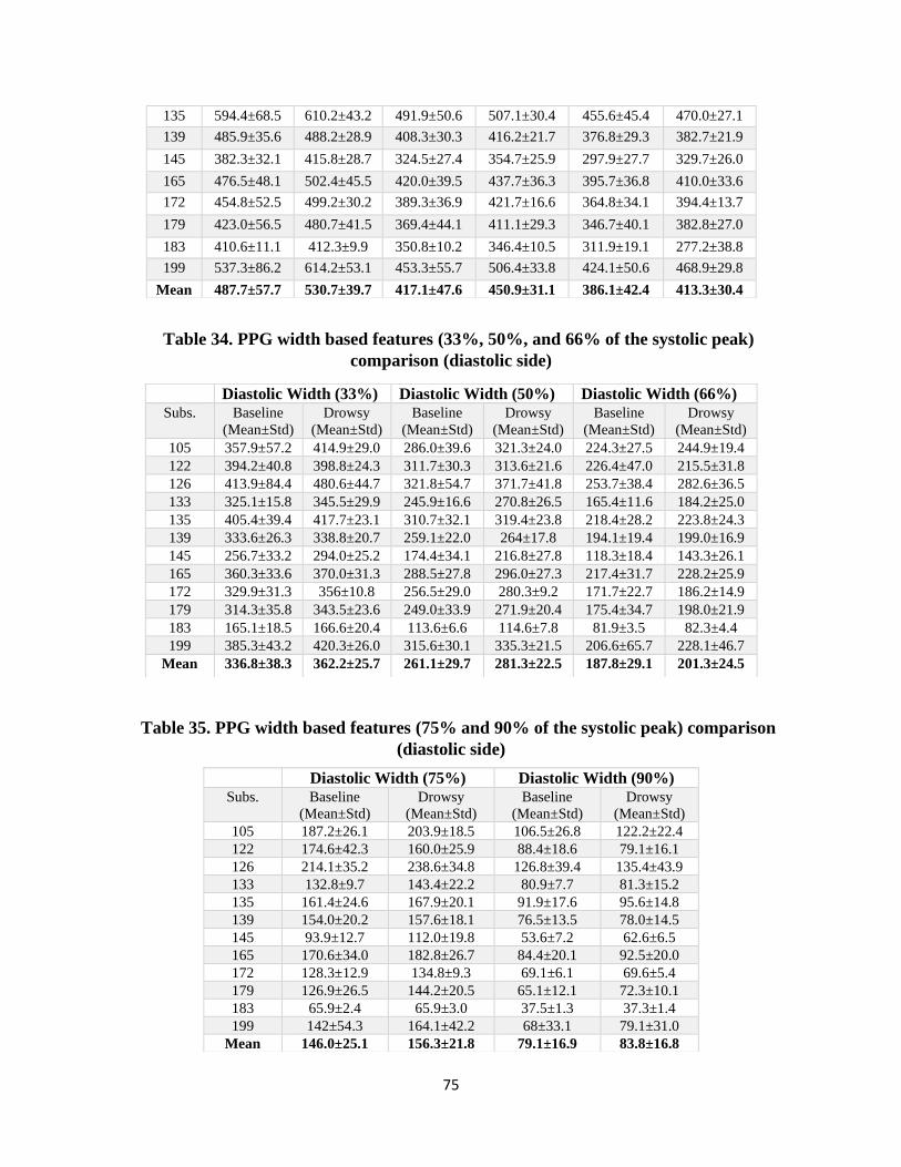
75

Table 34. PPG width based features (33%, 50%, and 66% of the systolic peak)

comparison (diastolic side)

Table 35. PPG width based features (75% and 90% of the systolic peak) comparison

(diastolic side)

135 594.4±68.5 610.2±43.2 491.9±50.6 507.1±30.4 455.6±45.4 470.0±27.1

139 485.9±35.6 488.2±28.9 408.3±30.3 416.2±21.7 376.8±29.3 382.7±21.9

145 382.3±32.1 415.8±28.7 324.5±27.4 354.7±25.9 297.9±27.7 329.7±26.0

165 476.5±48.1 502.4±45.5 420.0±39.5 437.7±36.3 395.7±36.8 410.0±33.6

172 454.8±52.5 499.2±30.2 389.3±36.9 421.7±16.6 364.8±34.1 394.4±13.7

179 423.0±56.5 480.7±41.5 369.4±44.1 411.1±29.3 346.7±40.1 382.8±27.0

183 410.6±11.1 412.3±9.9 350.8±10.2 346.4±10.5 311.9±19.1 277.2±38.8

199 537.3±86.2 614.2±53.1 453.3±55.7 506.4±33.8 424.1±50.6 468.9±29.8

Mean 487.7±57.7 530.7±39.7 417.1±47.6 450.9±31.1 386.1±42.4 413.3±30.4

Diastolic Width (33%) Diastolic Width (50%) Diastolic Width (66%)

Subs. Baseline

(Mean±Std)

Drowsy

(Mean±Std)

Baseline

(Mean±Std)

Drowsy

(Mean±Std)

Baseline

(Mean±Std)

Drowsy

(Mean±Std)

105 357.9±57.2 414.9±29.0 286.0±39.6 321.3±24.0 224.3±27.5 244.9±19.4

122 394.2±40.8 398.8±24.3 311.7±30.3 313.6±21.6 226.4±47.0 215.5±31.8

126 413.9±84.4 480.6±44.7 321.8±54.7 371.7±41.8 253.7±38.4 282.6±36.5

133 325.1±15.8 345.5±29.9 245.9±16.6 270.8±26.5 165.4±11.6 184.2±25.0

135 405.4±39.4 417.7±23.1 310.7±32.1 319.4±23.8 218.4±28.2 223.8±24.3

139 333.6±26.3 338.8±20.7 259.1±22.0 264±17.8 194.1±19.4 199.0±16.9

145 256.7±33.2 294.0±25.2 174.4±34.1 216.8±27.8 118.3±18.4 143.3±26.1

165 360.3±33.6 370.0±31.3 288.5±27.8 296.0±27.3 217.4±31.7 228.2±25.9

172 329.9±31.3 356±10.8 256.5±29.0 280.3±9.2 171.7±22.7 186.2±14.9

179 314.3±35.8 343.5±23.6 249.0±33.9 271.9±20.4 175.4±34.7 198.0±21.9

183 165.1±18.5 166.6±20.4 113.6±6.6 114.6±7.8 81.9±3.5 82.3±4.4

199 385.3±43.2 420.3±26.0 315.6±30.1 335.3±21.5 206.6±65.7 228.1±46.7

Mean 336.8±38.3 362.2±25.7 261.1±29.7 281.3±22.5 187.8±29.1 201.3±24.5

Diastolic Width (75%) Diastolic Width (90%)

Subs. Baseline

(Mean±Std)

Drowsy

(Mean±Std)

Baseline

(Mean±Std)

Drowsy

(Mean±Std)

105 187.2±26.1 203.9±18.5 106.5±26.8 122.2±22.4

122 174.6±42.3 160.0±25.9 88.4±18.6 79.1±16.1

126 214.1±35.2 238.6±34.8 126.8±39.4 135.4±43.9

133 132.8±9.7 143.4±22.2 80.9±7.7 81.3±15.2

135 161.4±24.6 167.9±20.1 91.9±17.6 95.6±14.8

139 154.0±20.2 157.6±18.1 76.5±13.5 78.0±14.5

145 93.9±12.7 112.0±19.8 53.6±7.2 62.6±6.5

165 170.6±34.0 182.8±26.7 84.4±20.1 92.5±20.0

172 128.3±12.9 134.8±9.3 69.1±6.1 69.6±5.4

179 126.9±26.5 144.2±20.5 65.1±12.1 72.3±10.1

183 65.9±2.4 65.9±3.0 37.5±1.3 37.3±1.4

199 142±54.3 164.1±42.2 68±33.1 79.1±31.0

Mean 146.0±25.1 156.3±21.8 79.1±16.9 83.8±16.8

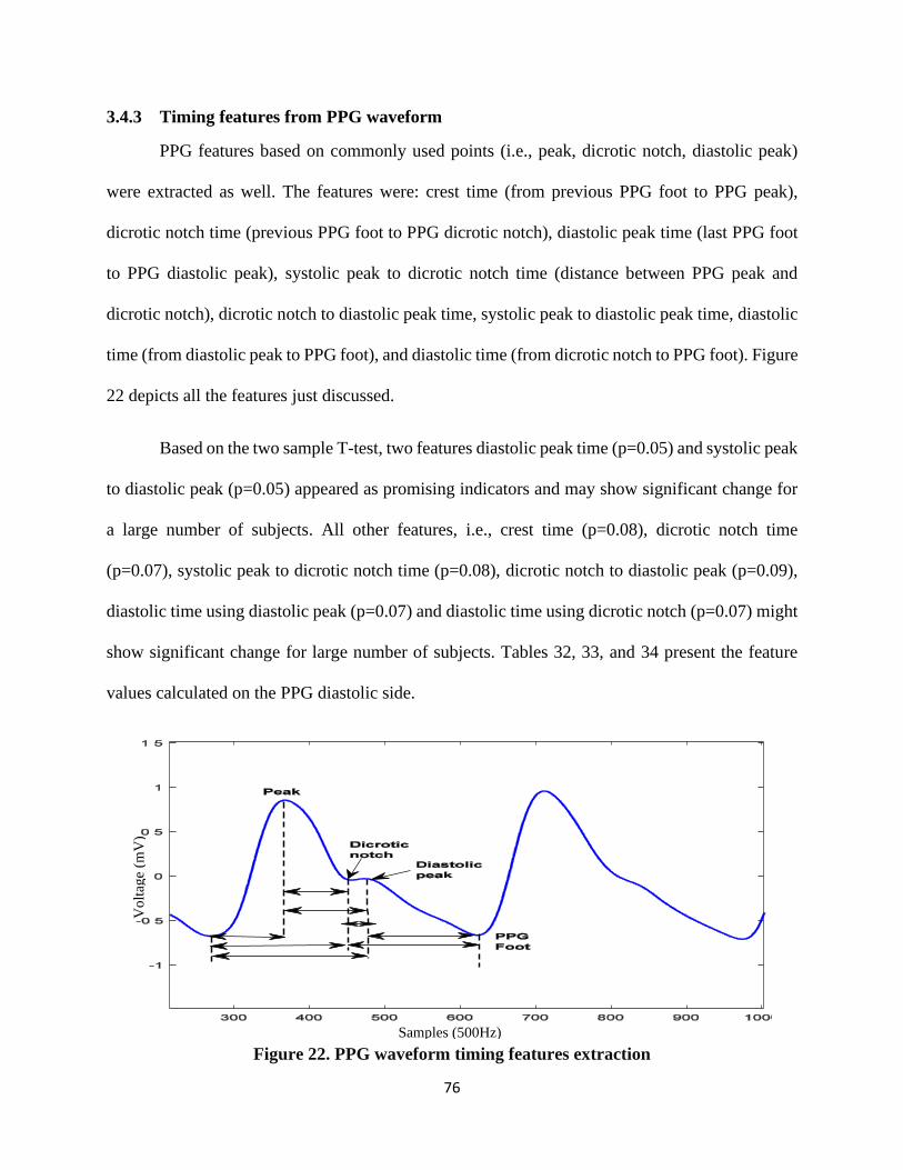
76

3.4.3 Timing features from PPG waveform

PPG features based on commonly used points (i.e., peak, dicrotic notch, diastolic peak)

were extracted as well. The features were: crest time (from previous PPG foot to PPG peak),

dicrotic notch time (previous PPG foot to PPG dicrotic notch), diastolic peak time (last PPG foot

to PPG diastolic peak), systolic peak to dicrotic notch time (distance between PPG peak and

dicrotic notch), dicrotic notch to diastolic peak time, systolic peak to diastolic peak time, diastolic

time (from diastolic peak to PPG foot), and diastolic time (from dicrotic notch to PPG foot). Figure

22 depicts all the features just discussed.

Based on the two sample T-test, two features diastolic peak time (p=0.05) and systolic peak

to diastolic peak (p=0.05) appeared as promising indicators and may show significant change for

a large number of subjects. All other features, i.e., crest time (p=0.08), dicrotic notch time

(p=0.07), systolic peak to dicrotic notch time (p=0.08), dicrotic notch to diastolic peak (p=0.09),

diastolic time using diastolic peak (p=0.07) and diastolic time using dicrotic notch (p=0.07) might

show significant change for large number of subjects. Tables 32, 33, and 34 present the feature

values calculated on the PPG diastolic side.

Figure 22. PPG waveform timing features extraction

Samples (500Hz)

Vo

ltag

e (m

V)

77

Table 36. PPG features (crest time, dicrotic notch time, and diastolic peak time)

comparison for baseline and drowsy periods

Table 37. PPG features (systolic peak to dicrotic notch time, dicrotic notch to diastolic

peak, and systolic peak to diastolic peak) comparison for baseline and drowsy periods

Crest time Dicrotic notch time Diastolic peak time Subs. Baseline

(Mean±Std)

Drowsy

(Mean±Std)

Baseline

(Mean±Std)

Drowsy

(Mean±Std)

Baseline

(Mean±Std)

Drowsy

(Mean±Std)

105 263.1±19.8 325.9±38.4 498.9±199.6 752.3±134.0 559.8±219.2 813.7±151.9

122 169.7±8.1 217.2±55.2 357.1±29 462.1±126.1 415.3±27.0 525.1±126.7

126 285.5±18.4 320.8±82.2 559.4±177.9 684.7±234.9 611.4±194.8 744.0±224.0

133 204.8±12.5 226.6±40.1 429.4±82.3 435.6±83.4 484.5±84.9 508.5±78.2

135 244.8±22.2 323.0±56.3 546.9±115.8 755.5±132.8 610.6±128.1 817.8±136.4

139 263.5±17.3 273.4±17.5 536.2±99.4 590.7±105.2 596.3±111.3 655±125.1

145 177.6±10.6 220.6±17.5 331.3±46.3 388.8±85.0 404.1±64.0 451.7±98.3

165 181.4±20.1 227.2±40.4 335.8±63.7 433.8±150.6 403.1±84.3 499.3±151.3

172 219.1±17.4 196.2±7.4 429.7±78.7 374.1±24.8 483.5±80.2 451.4±20.6

179 219.6±26.3 253.9±27.2 364.0±101.9 465.0±119.1 419.8±88.7 529.2±112.1

183 202.3±16.2 224.9±41.1 400.1±42.2 433.8±58.8 467.2±46.9 502.9±60.7

199 167.8±10.6 192.2±31.3 327.2±84.6 420.3±90.0 394.3±84.7 491.1±88.9

Mean 216.6±16.6 250.2±37.9 426.3±93.4 516.4±112.1 487.5±101.2 582.5±114.5

Systolic peak to dicrotic

notch time

Dicrotic notch to

diastolic peak

Systolic peak to diastolic

peak

Subs. Baseline

(Mean±Std)

Drowsy

(Mean±Std)

Baseline

(Mean±Std)

Drowsy

(Mean±Std)

Baseline

(Mean±Std)

Drowsy

(Mean±Std)

105 235.7±189.1 426.3±124.6 57.3±40.6 60.1±38.8 296.3±208.1 488.2±143.6

122 187.3±28.9 244.9±93.4 58.1±21.0 62.9±21.0 245.5±27.2 307.8±94.3

126 273.9±176.4 363.8±192.2 51.9±31.6 59.3±27.6 325.8±193.2 423.2±185.9

133 224.6±85.2 209±83.8 53.6±29.4 65.7±19.3 279.7±87.7 277.8±86.4

135 302.0±108.8 432.5±119.4 63.7±31.2 56.6±25.7 365.8±123.7 494.1±124.8

139 272.6±98.1 317.2±106.1 60.1±29.8 64.2±39.1 332.7±110.4 381.5±126.3

145 153.6±45.2 168.1±86.1 72.7±28.2 65.4±25.7 226.6±63.1 232.1±100.6

165 154.3±62.6 206.6±138.4 67.3±40.3 65.2±28.9 221.7±82.4 271.9±138.9

172 210.6±75.7 177.9±22.6 54.7±29.2 77.2±29.1 264.9±77.9 255.2±23.4

179 144.3±96.6 211.0±110.9 55.8±37.0 64.2±31.3 200.2±83.4 275.2±106.2

183 197.7±37.5 208.9±37.3 66.1±28.1 69.0±31.2 264.9±41.0 277.9±42.6

199 159.4±83.9 228.1±83.2 67.1±36.6 70.1±24.1 226.5±84.8 298.7±83.4

Mean 209.7±90.7 266.2±99.8 60.7±31.9 65.0±28.5 270.9±98.6 332.0±104.7

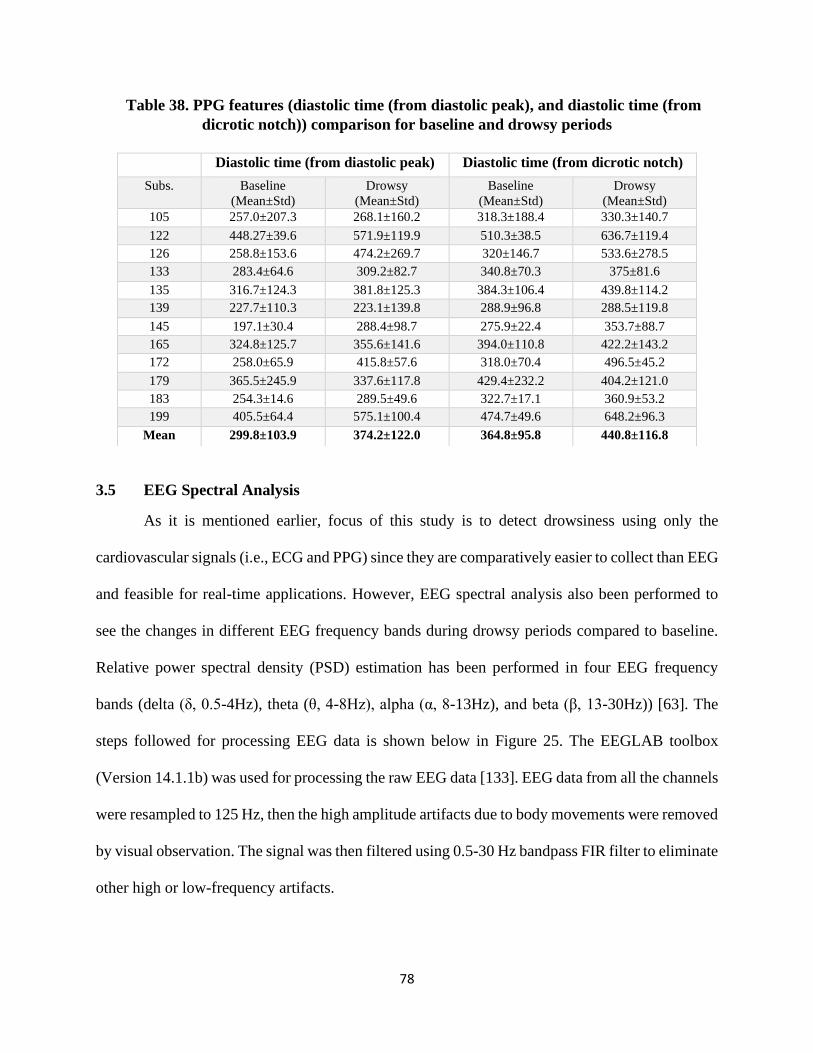
78

Table 38. PPG features (diastolic time (from diastolic peak), and diastolic time (from

dicrotic notch)) comparison for baseline and drowsy periods

3.5 EEG Spectral Analysis

As it is mentioned earlier, focus of this study is to detect drowsiness using only the

cardiovascular signals (i.e., ECG and PPG) since they are comparatively easier to collect than EEG

and feasible for real-time applications. However, EEG spectral analysis also been performed to

see the changes in different EEG frequency bands during drowsy periods compared to baseline.

Relative power spectral density (PSD) estimation has been performed in four EEG frequency

bands (delta (δ, 0.5-4Hz), theta (θ, 4-8Hz), alpha (α, 8-13Hz), and beta (β, 13-30Hz)) [63]. The

steps followed for processing EEG data is shown below in Figure 25. The EEGLAB toolbox

(Version 14.1.1b) was used for processing the raw EEG data [133]. EEG data from all the channels

were resampled to 125 Hz, then the high amplitude artifacts due to body movements were removed

by visual observation. The signal was then filtered using 0.5-30 Hz bandpass FIR filter to eliminate

other high or low-frequency artifacts.

Diastolic time (from diastolic peak) Diastolic time (from dicrotic notch)

Subs. Baseline

(Mean±Std)

Drowsy

(Mean±Std)

Baseline

(Mean±Std)

Drowsy

(Mean±Std)

105 257.0±207.3 268.1±160.2 318.3±188.4 330.3±140.7

122 448.27±39.6 571.9±119.9 510.3±38.5 636.7±119.4

126 258.8±153.6 474.2±269.7 320±146.7 533.6±278.5

133 283.4±64.6 309.2±82.7 340.8±70.3 375±81.6

135 316.7±124.3 381.8±125.3 384.3±106.4 439.8±114.2

139 227.7±110.3 223.1±139.8 288.9±96.8 288.5±119.8

145 197.1±30.4 288.4±98.7 275.9±22.4 353.7±88.7

165 324.8±125.7 355.6±141.6 394.0±110.8 422.2±143.2

172 258.0±65.9 415.8±57.6 318.0±70.4 496.5±45.2

179 365.5±245.9 337.6±117.8 429.4±232.2 404.2±121.0

183 254.3±14.6 289.5±49.6 322.7±17.1 360.9±53.2

199 405.5±64.4 575.1±100.4 474.7±49.6 648.2±96.3

Mean 299.8±103.9 374.2±122.0 364.8±95.8 440.8±116.8

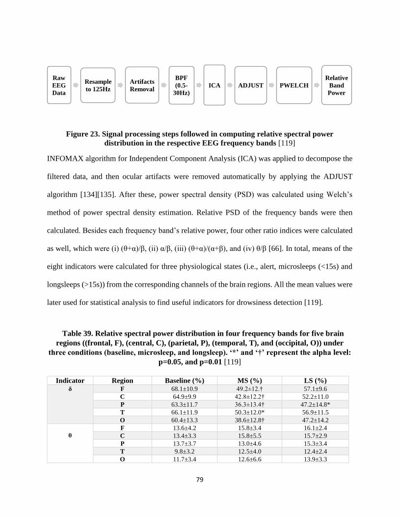
79

Figure 23. Signal processing steps followed in computing relative spectral power

distribution in the respective EEG frequency bands [119]

INFOMAX algorithm for Independent Component Analysis (ICA) was applied to decompose the

filtered data, and then ocular artifacts were removed automatically by applying the ADJUST

algorithm [134][135]. After these, power spectral density (PSD) was calculated using Welch’s

method of power spectral density estimation. Relative PSD of the frequency bands were then

calculated. Besides each frequency band’s relative power, four other ratio indices were calculated

as well, which were (i) (θ+α)/β, (ii) α/β, (iii) (θ+α)/(α+β), and (iv) θ/β [66]. In total, means of the

eight indicators were calculated for three physiological states (i.e., alert, microsleeps (<15s) and

longsleeps (>15s)) from the corresponding channels of the brain regions. All the mean values were

later used for statistical analysis to find useful indicators for drowsiness detection [119].

Table 39. Relative spectral power distribution in four frequency bands for five brain

regions ((frontal, F), (central, C), (parietal, P), (temporal, T), and (occipital, O)) under

three conditions (baseline, microsleep, and longsleep). ‘*’ and ‘†’ represent the alpha level:

p=0.05, and p=0.01 [119]

Indicator Region Baseline (%) MS (%) LS (%) δ F 68.1±10.9 49.2±12.† 57.1±9.6

C 64.9±9.9 42.8±12.2† 52.2±11.0

P 63.3±11.7 36.3±13.4† 47.2±14.8*

T 66.1±11.9 50.3±12.0* 56.9±11.5

O 60.4±13.3 38.6±12.8† 47.2±14.2

θ

F 13.6±4.2 15.8±3.4 16.1±2.4

C 13.4±3.3 15.8±5.5 15.7±2.9

P 13.7±3.7 13.0±4.6 15.3±3.4

T 9.8±3.2 12.5±4.0 12.4±2.4

O 11.7±3.4 12.6±6.6 13.9±3.3

Raw

EEG

Data

Resample

to 125Hz

Artifacts

Removal

BPF

(0.5-

30Hz)

ICA ADJUST PWELCH

Relative

Band

Power

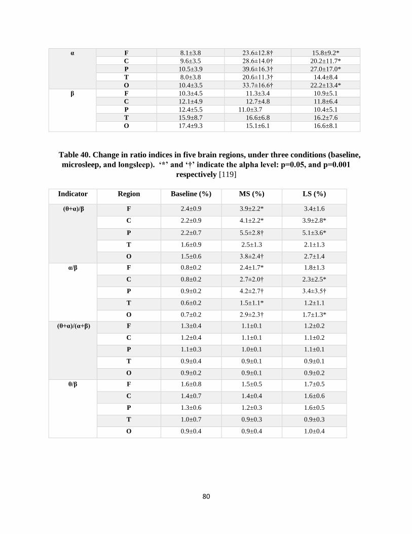
80

α F 8.1±3.8 23.6±12.8† 15.8±9.2*

C 9.6±3.5 28.6±14.0† 20.2±11.7*

P 10.5±3.9 39.6±16.3† 27.0±17.0*

T 8.0±3.8 20.6±11.3† 14.4±8.4

O 10.4±3.5 33.7±16.6† 22.2±13.4*

β F 10.3±4.5 11.3±3.4 10.9±5.1

C 12.1±4.9 12.7±4.8 11.8±6.4

P 12.4±5.5 11.0±3.7 10.4±5.1

T 15.9±8.7 16.6±6.8 16.2±7.6

O 17.4±9.3 15.1±6.1 16.6±8.1

Table 40. Change in ratio indices in five brain regions, under three conditions (baseline,

microsleep, and longsleep). ‘*’ and ‘†’ indicate the alpha level: p=0.05, and p=0.001

respectively [119]

Indicator Region Baseline (%) MS (%) LS (%)

(θ+α)/β F 2.4±0.9 3.9±2.2* 3.4±1.6

C 2.2±0.9 4.1±2.2* 3.9±2.8*

P 2.2±0.7 5.5±2.8† 5.1±3.6*

T 1.6±0.9 2.5±1.3 2.1±1.3

O 1.5±0.6 3.8±2.4† 2.7±1.4

α/β F 0.8±0.2 2.4±1.7* 1.8±1.3

C 0.8±0.2 2.7±2.0† 2.3±2.5*

P 0.9±0.2 4.2±2.7† 3.4±3.5†

T 0.6±0.2 1.5±1.1* 1.2±1.1

O 0.7±0.2 2.9±2.3† 1.7±1.3*

(θ+α)/(α+β) F 1.3±0.4 1.1±0.1 1.2±0.2

C 1.2±0.4 1.1±0.1 1.1±0.2

P 1.1±0.3 1.0±0.1 1.1±0.1

T 0.9±0.4 0.9±0.1 0.9±0.1

O 0.9±0.2 0.9±0.1 0.9±0.2

θ/β F 1.6±0.8 1.5±0.5 1.7±0.5

C 1.4±0.7 1.4±0.4 1.6±0.6

P 1.3±0.6 1.2±0.3 1.6±0.5

T 1.0±0.7 0.9±0.3 0.9±0.3

O 0.9±0.4 0.9±0.4 1.0±0.4

81

Our analysis showed that the delta band (0.5-4Hz) power decreases significantly during

microsleeps (all the brain regions) and longsleeps (frontal and parietal) compared to baseline.

Alpha band (8-13Hz) power increases significantly during microsleeps (all the brain regions) and

longsleeps (except temporal region) compared to baseline. In the case of ratio indices, (θ+α)/β

showed significant increases during microsleeps (except temporal region) and longsleeps (except

temporal and occipital) compared to baseline. Besides, α/β showed a substantial increase during

microsleeps (all the brain regions) and longsleeps (except frontal and temporal) compared to

baseline. Figures 24 and 25 depict the changes of different indicators during three

psychophysiological states (i.e., baseline, microsleeps, and longsleeps).

Figure 24. Relative spectral power distribution (mean±SE) in four EEG frequency bands: δ,

θ, α, and β during three psychological states (baseline (BL), microsleeps (MS), and longsleeps

(LS)) in five brain regions ((Frontal, F), (Central, C), (Parietal, P), (Temporal, T), and

(Occipital, O)). The x-axis represents three psychological states, and the y-axis represents

relative PSD [119]

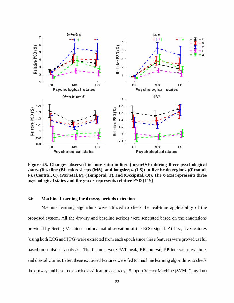
82

Figure 25. Changes observed in four ratio indices (mean±SE) during three psychological

states (Baseline (BL microsleeps (MS), and longsleeps (LS)) in five brain regions ((Frontal,

F), (Central, C), (Parietal, P), (Temporal, T), and (Occipital, O)). The x-axis represents three

psychological states and the y-axis represents relative PSD [119]

3.6 Machine Learning for drowsy periods detection

Machine learning algorithms were utilized to check the real-time applicability of the

proposed system. All the drowsy and baseline periods were separated based on the annotations

provided by Seeing Machines and manual observation of the EOG signal. At first, five features

(using both ECG and PPG) were extracted from each epoch since these features were proved useful

based on statistical analysis. The features were PAT-peak, RR interval, PP interval, crest time,

and diastolic time. Later, these extracted features were fed to machine learning algorithms to check

the drowsy and baseline epoch classification accuracy. Support Vector Machine (SVM, Gaussian)

83

achieved 90% accuracy in classification of drowsy and baseline epochs (AUC=0.89, 25% held

out).

Then only PPG based features were extracted and checked to see whether it is possible to

detect drowsiness using only the PPG signal since PPG is much easier to collect than ECG and

EEG, as well as feasible for real-time wearable applications. Eight features, (crest time, dicrotic

notch time, diastolic peak time, dicrotic notch to systolic peak, diastolic peak to dicrotic notch,

diastolic peak to systolic peak, diastolic time (from diastolic peak), and diastolic time (from

dicrotic notch)) were extracted from each subject PPG signal. In this case the classification

accuracy was 87% using SVM (Gaussian, AUC=0.91, 5-fold Cross-validation). Though overall

classification accuracy reduced, it indicates that using only PPG features it is possible to classify

the drowsy epochs with satisfactory accuracy.

In another approach, instead of dealing with all the subjects’ drowsy and baseline epochs

at the same time, leave-one-out cross-validation procedure was applied. One subject was excluded

from the classifier model training; once the model was trained with rest of the subjects (n-1

subjects, where n is total number of subjects), it was then used to classify the drowsy and baseline

epochs on that subject. This procedure was repeated n times. In this way the classifier performed

well for drowsy epochs detection with an average accuracy of 75.8% (SVM (Gaussian)); for some

subjects, the drowsy epoch detection accuracy was more than 90%.

84

CHAPTER 04

DISCUSSION

Operating an aircraft or driving a vehicle is an intricate task which requires flying or driving

skill, high attention, rapid decision-making capability, planning, visual perception, and object

detection ability [136]. Drowsiness reduces the attention level and increases the reaction time,

which is responsible for a vast amount of accidents occur every year. Physiological signals based

continuous vigilance state monitoring and on-time warning can help in reducing the number of

accidents happen due to drowsiness.

Among the commonly used physiological signals, EEG is the most used one followed by

the ECG, whereas EOG is mainly used as the gold standard to verify the drowsy periods since this

signal is directly related to the eye closure and opening. Based on the previous studies, though

PPG is easily obtainable compared to EEG and ECG, it is not used by many research groups for

drowsiness detection applications. In this study, the feasibility of the cardiovascular signals,

especially PPG has been checked, whether it is able to detect drowsiness without other signals or

with the help of another easily obtainable signal, like ECG. Hence, both ECG and PPG signals

behavior were studied to check their usability for drowsiness detection. Heart rate variability, pulse

rate variability, pulse arrival time, morphological, timing, width, and height-based features were

studied to check whether there are any significant changes happen during drowsy periods

compared to alert periods.

For ECG, different signal length based HRV analysis was performed, such as HRV using

5 min windowing, 3 min windowing, ultra-short HRV using 30 seconds windowing. HRV features,

including heart rate, SDNN, SDSD, NN50, PNN50, RMSSD, VLF (%), LF (%), HF (%), and

LF/HF were calculated for 5 min data windowing (see Table 9, 10, 11 and 12). Heart rate

85

decreased for all the subjects during drowsy periods (76.34±0.33) compared to baseline or alert

periods (80.44±0.42). Also, LF (35.51±3.31 for baseline vs. 30.55±3.13 for drowsy periods), RLH

(0.79±0.17 for baseline vs. 0.64±0.14 for drowsy periods) decreased during drowsy periods

compared to baseline. In contrast, SDNN (106.66±10.34 vs. 170.73±6.05), SDSD (145.85±17.91

vs. 246.68±11.29), NN50, PNN50, RMSSD, VLF, and HF showed increased value during

drowsiness compared to baseline. However, based on statistical analysis (two-sample t-test), only

SDNN, SDSD, and RMSSD showed significant change during drowsy periods compared to alert

periods.

HRV analysis using 3 min windowing has been performed as well, but this time the focus

was not the drowsy periods, instead the periods before the first drowsy period was focused. The

goal behind this approach was to check whether there was any significant change in signal behavior

just before the first drowsy period. Previously mentioned features were calculated along with

NN20, PNN20, NN10, PNN10, absolute power of LF and HF band (see Table 13, 14, 15, 16, and

17). Heart rate, SDSD, RMSSD, NN20, PNN20, NN10, PNN10, HF (absolute power) and HF

(%) showed decreased value before the first drowsy period compared to baseline. In contrast

SDNN, NN50, PNN50, LF, and LF/HF showed increased value during the periods before the first

drowsy period. However, none of the features showed significant (based on two sample t-test)

changes during the period before the first drowsy period compared to baseline periods.

Ultra-short HRV analysis was applied using 30s data segmentation to check the feasibility

of early drowsiness detection. For this, first 30s of a drowsy period are compared to the baseline

periods. HRV features including, heart rate, SDNN, SDSD, RMSSD, NN50, PNN50, LF (%), HF

(%), LF (absolute power), HF (absolute power) and LF/HF ratio were calculated (see Table 18,

19, 20, and 21). Heart rate decreased during drowsy periods; the same is applicable for LF (%) and

86

LF/HF ratio. Whereas SDNN, SDSD, RMSSD, NN50, PNN50, HF (%), LF (absolute power), and

HF (absolute power) increased during drowsy periods. However, based on statistical analysis (two-

sample t-test) only SDNN, LF (absolute), and HF (absolute) showed significant change. The

changes could happen due to the decrease in sympathetic activities and increase in parasympathetic

activities during drowsy periods. In contrast, for the baseline periods, sympathetic activity was

high compared to parasympathetic activity due to the subject’s involvement with flight operation.

Pulse rate variability (PRV) using the PPG signal was performed to check whether the PRV

behavior is similar to ECG based HRV analysis. PRV with 5-minute data segmentation was used

to calculate pulse rate, SDNN, SDSD, RMSSD, NN50, PNN50, VLF (%), LF (%), HF (%) and

LF/HF feature (see Table 22, 23, 24, 25). Based on two sample t-test, none of the features showed

significant (p<0.05) change. However, the p-value for SDNN (p=0.057), SDSD (p=0.06), and

RMSSD (p=0.06) indicate that for a larger population these features might show significant change

during drowsiness compared to alert or baseline periods.

In the case of the correlation between the PRV and HRV features, some of the time domain

features showed a high correlation, whereas most of the frequency domain features were not.

Previous studies showed that both HRV and PRV showed significant correlation when the subjects

are in rest condition especially in supine position. On the other hand, for active condition the

correlations are not high and consistent [132]. Our study was performed in an active mode, i.e.,

subjects were requested to perform a routine flight operation using a flying simulator, which

influenced the correlation between HRV and PRV analysis.

Pulse arrival time (PAT) was calculated using both ECG and PPG signals. PAT is the time

delay between the ECG R-peak and a specific point (e.g., peak, foot, first derivative peak, second

derivative peak) on the PPG waveform (see Figure 13). ECG R–peak is used as the proximal point

87

and another point in PPG waveform is used as the distal point. Besides PAT, RR interval, and PP

intervals were calculated for each PPG waveform in selected drowsy periods (15s to 35s). PAT/RR

was calculated for each epoch to see whether the change in pulse arrival time is only influenced

by RR interval changes during drowsy periods due to the decreased sympathetic activity and

increased parasympathetic activity (see Table 26 and 27). PPG peak based PAT (PAT-peak,

p=0.04), RR interval (p=0.004), and PP interval (p=0.005) showed significant change during

drowsiness. PAT-peak showed a significant (p<0.05) increase during drowsy periods

(443.51±14.07ms) compared to alert periods (407.66±9.85ms) [11]. All the subjects (12 for this

analysis) showed an increase in PAT during drowsiness (Figure 26). For RR interval the mean was

781.87±29.48ms during baseline and 958.78±61.74ms for drowsy periods. PP interval mean was

similar to RR interval, 783.75±32.16ms for baseline vs. 960.22±66.85ms for drowsy periods. All

the subjects showed increased RR and PP intervals during drowsy periods compared to alert

periods (Figure 17 and Figure 18).

In the case of PAT/RR, the p-value was 0.06, which is not significant based on our

threshold (p<0.05) for being significant. However, it indicates that PAT/RR can show significant

changes for a large number of subjects. Also, PAT/RR showed the opposite behavior of both PAT

and RR interval (Figure 17). The decrease in PAT/RR during drowsy periods for most of the

subjects (9 out of 12) indicates that increase in pulse arrival time is not solely influenced by the

heart rate changes instead some other factors like arterial stiffness could play a role. It also

indicates that PAT/RR can be used as an independent feature for drowsiness detection since

commonly used heart rate can fluctuate for many others physiological factors (e.g., stress, pain,

hormones, medication) and environmental factors (e.g., temperature), as well as independent of

age.

88

Though PPG foot is the conventional and mostly used point for PAT calculation [137],

[138], there are studies that used other points for PAT calculation as well. For example, Chua and

Heneghan used ECG R-peak and the point with the highest gradient on the upward edge of the

PPG for PAT calculation [139], Baek et al. used PPG first derivative [140], Rajala et al. used PPG

peak, foot, first and second derivative peak [121], PPG peak, foot, 20% height, and the maximum

first derivative was used by another group [141]. As mentioned earlier, we used three other

measures (i.e., ECG R peak to PPG foot, first derivative peak, and second derivative peak) for

PAT calculation (see Table 28, Figures 19 and 20). PAT based on PPG foot reduced for most of

the subjects with a group mean of 176.89±20.72ms for drowsy periods compared to

178.18±10.96ms for baseline periods. Both PATs based on the first derivative peak and second

derivative peak increased during drowsy periods compared to baseline periods, PAT- first

derivative (299.44±7.32ms vs. 284.39±5.2ms) and PAT-second derivative (244.27±8.55ms vs.

229.64±6.87ms). However, none of them should significant (p<0.05) change based on statistical

analysis (two-sample t-test), PAT-foot (p=0.88), PAT- first derivative (p=0.10) and PAT-second

derivative (p=0.11). Based on their current p values, PAT-first derivative and PAT-second

derivative might show significant change for a large number of subjects.

Based on our analysis, PPG peak based PAT is highly promising (compared to three other

methods) and showed significant change during drowsiness. Moreover, PPG peak based PATs are

easy to calculate and computationally less expensive. As mentioned earlier, ear PPG had been used

for signal acquisition, this spot (i.e., earlobe) is proved to be less sensitive to age and height

compared to other commonly used PPG acquisition spots (e.g., fingers, toes) [142]. Since our

participants’ age range was not wide (21±2.4 years), the ear PAT should not be affected due to age

89

variation. Though heart rate, which is independent of age, affects ear PAT, study showed it is not

significant [142].

Since one of the goals of our study was to check the feasibility of a single signal (especially

PPG) for drowsiness detection, only PPG based features were extracted as well, such as PPG

morphological and width based features. At first, commonly used features, like systolic amplitude,

crest time, pulse interval, pulse interval/systolic amplitude, and diastolic time features were

calculated (see Table 29 and 30). Except decrease in systolic amplitude during drowsiness

compared to baseline periods (1.13±0.14 vs. 1.38±0.13), other features showed increased values

during drowsiness compared to baseline, such as crest time (271.78±32.31ms vs. 230.15±15.9ms),

pulse interval (957.96±69.94ms vs. 789.43±36.85ms), pulse interval/systolic amplitude

(1333.9±159.04 vs. 885.46±101.86) and diastolic time (686.55±54.36ms vs. 559.49±28.97ms).

Among these features, based on two sample t-test three features showed the potential (p<0.05) to

discriminate drowsy and baseline periods, the features are crest time (p=0.047), pulse interval

(p=0.007), and diastolic time (p=0.009). 11 out of 12 subjects showed increased mean values for

crest time and diastolic time during drowsy periods (see Figure 22), which might happen due to

the extended pulse waveform during drowsy periods, resulting in wider crest time and diastolic

time. Two other features, systolic amplitude (p=0.55) and pulse interval/systolic amplitude

(p=0.239) did not show any significant changes. These two features might show significant change

for larger subject size.

PPG waveform width features from both systolic and diastolic side were calculated as well,

using a gradual increase in height (e.g., width at 10% or 20% height). The features were systolic

width and diastolic width at 10%, 20%, 25%, 33%, 50%, 66%, 75%, and 90% height (see Figure

23, Table 31, 32, 33, 34, 35 and 36). The assumption was since there was an increase in crest time

90

(time between a PPG foot to the immediate next PPG systolic peak) and diastolic time (time

between a systolic peak to its immediate next PPG foot), PPG waveform widths at different points

should increase as well. All the features showed increased value for drowsy periods compared to

alert periods. However, based on the statistical test (two-sample t-test), none of the features

appeared as a potential indicator (p<0.05). This implies that, though there is an increase in crest

time during drowsiness, the increased duration is not evenly distributed at different points of PPG

width, and it varies subject to subject.

PPG based timing features were calculated using commonly used and apparent PPG peaks

and notches, i.e., systolic peak, diastolic peak, dicrotic notch, and foot (see Figure 24). The

calculated features were: crest time (from previous PPG foot to immediate next PPG peak), dicrotic

notch time (previous PPG foot to immediate next PPG dicrotic notch point), diastolic peak time

(previous PPG foot to immediate next PPG diastolic peak), systolic peak to dicrotic notch time

(distance between PPG peak/systolic peak and dicrotic notch point), dicrotic notch to diastolic

peak time, systolic peak to diastolic peak time, diastolic time1 (from diastolic peak to immediate

next PPG foot), and diastolic time2 (from dicrotic notch to immediate next PPG foot) (see Table

37, 38, and 39). All the features' value increased during drowsiness compared to baseline periods.

Based on the two sample t-test, two features diastolic peak time (p<0.05) and systolic peak to

diastolic peak (p<0.05) showed a significant increase during drowsiness. All other features i.e.,

crest time (p=0.08), dicrotic notch time (p=0.07), systolic peak to dicrotic notch time (p=0.08),

dicrotic notch to diastolic peak (p=0.09), diastolic time using diastolic peak (p=0.07) and diastolic

time using dicrotic notch (p=0.07) might show significant change for large number of subjects and

can be used as indicators of drowsiness. However, if the signal quality is not good, and some of

the desired points in PPG waveform (like dicrotic notch, diastolic peak) are not apparent like the

91

systolic peak and foot, (appearance of these points also influenced by the subject’s age) it is better

to avoid the features related to these points instead of a wrong estimation.

To investigate the pilot's EEG behavior within the window of circadian low, our

experiment was conducted from 2:00 AM to 4:30 AM, and the initial 3-5 minutes of simulated

flight was chosen as the baseline. Participants were awake for 18-20 hours before they appeared

for the study; therefore, they were already into the early stage of drowsiness before starting the

experiment. This is in good agreement with the ratings of the KSS assessment. Average pre-flight

KSS value of 5.4 corroborates our statement that the pilots seem to have some signs of sleepiness

[143]. Additionally, in the literature, there are no set criteria for "microsleep" and the authors used

a variety of definitions and measurements [28]. Therefore, we set sleep duration from 1.5-15s as

MS and greater than 15s as LS for this study [18].

For EEG analysis, power spectral density (PSD) estimation was applied. Relative band

power changes during microsleep (MS, <15s) and longesleep (LS, >15s) periods compared to

baseline periods were calculated for four EEG frequency bands (delta (δ, 0.5-4Hz), theta (θ, 4-

8Hz), alpha (α, 8-13Hz), and beta (β, 13-30Hz)) from five brain regions ((Frontal, F), (Central, C),

(Parietal, P), (Temporal, T), and (Occipital, O)) (see Figure 25 and 26, Table 40). Besides power

in four frequency bands, four other ratio indices using these four frequency bands power ((θ+α)/β,

α/β, (θ+α)/(α+β) and θ/β) were calculated as well (see Table 41). For EEG, in existing literature,

researchers have found a significant change in delta and theta power, more specifically, in theta

power during drowsy state [63] [144] [145]. In a study of simulated driving, it was found that theta

power increased significantly during nighttime compared to baseline taken during daytime [146].

Another study on prolonged awakening revealed that theta power showed a significant increase

only at 9th, 21th, and 24th hours [147]. In our experiment for two hours of simulated flight, delta

92

power had a significant (p<0.05) decrease in all regions during microsleep (MS) as well as in

parietal region for longesleep (LS), while theta and beta power had no significant change [119]. A

similar result for delta activity has been reported in a monotonous simulated driving where total

driving time was segmented into 10 equal sections to identify changes in EEG spectra. Their result

showed a significant decrease in sections 6, 8 and 10 compared to section 4 in terms of delta

activity [148]. In the literature, alpha activity has been shown to be associated with microsleep

[134][149]. Gharagozlou et al. found a significant increase in absolute alpha power between the

first and the last 10 minutes of simulated driving sessions [150]. Papadelis et al. found a significant

increase in relative alpha power during drowsiness for on-road experiments [145]. Additionally,

other researchers revealed that alpha burst could be related to drowsiness [149][151]. These studies

comprehensively revealed that alpha activity is an important indicator of drowsiness. In our study,

we found that relative alpha band power showed a significant increase during MS (p<0.001, in all

regions), and LS (p<0.05, in all regions except temporal) compared to the baseline. Furthermore,

the alpha power has a decreasing but insignificant trend during LS compared to MS. These results

further confirm the importance of alpha band power in drowsiness assessment.

In the case of drowsy and alert periods classification using machine learning, combining

both ECG and PPG features showed better classification accuracy than relying on only PPG

features. Hence, it is recommended that both ECG and PPG should be used simultaneously for

better classification accuracy. However, in both cases, classification accuracy (>85%) indicates

that satisfactory classification of the drowsy and alert periods is possible using the cardiovascular

signals (ECG and PPG).

In the end, it can be mentioned, though EEG is the most studied physiological signal for

drowsiness detection, numerous electrodes placement on scalp made it impractical for on board

93

applications. Identification of the most useful electrode for drowsiness detection is another

challenge. However, a reduction in the number of electrodes and use of dry electrodes will play a

crucial role. On the other hand, other easily obtainable signals like ECG and PPG can be used for

drowsiness detection. Especially PPG should be extensively studied since it is much easier to

record and an excellent fit for wearable applications. ECG based HRV features are useful for

drowsiness estimation. However, for earlier detection the length of data needs to be shortened

which impacts the HRV analysis, and some of the HRV parameters are not useful for short time

window. In this case, PPG and ECG based PAT can play a substantial role since PAT can be

calculated from a short data length (as low as 5s, and for better reliability 10-15s). Besides PAT,

some other PPG based features like crest time, diastolic time, pulse interval, diastolic peak time,

and systolic peak to diastolic peak features showed significant change during drowsiness compared

to baseline periods. Hence, these features can be used for drowsiness detection and warning system

design. Other features, like dicrotic notch time, systolic peak to dicrotic notch time, dicrotic notch

to diastolic peak, diastolic time using diastolic peak, and diastolic time using dicrotic notch should

be studied as well.

Finally, for simple drowsiness detection and warning system design, the focus should be

on ECG and PPG. If the desired system is a headset like system, it is beneficial to include the EEG

as well; it might improve the overall drowsiness detection accuracy.

94

CHAPTER 05

CONCLUSION, FUTURE WORK, AND CONTRIBUTION

5.1 Conclusion

Based on our analysis, it is evident that the physiological signals are beneficial for early

and precise drowsiness detection. Among the signals we have recorded, EOG was used as the gold

standard to verify the eye closure which was further verified with video monitoring and the

researcher participated in data recording. EEG is the most widely used physiological signal for

drowsiness study; it has some parameters which showed significant change during drowsiness

compared to alert periods. In our study, relative spectral power in four EEG frequency bands, i.e.,

delta, theta, alpha, and beta band was calculated for five brain regions (i.e., frontal, central,

temporal, parietal and occipital). We found that delta band power reduced significantly (p<0.05)

during microsleep periods, and alpha power showed a significant increase during microsleep

events for all the brain regions. Theta and beta band power did not show any significant change

during drowsiness. However, one of the goals of this study was to check the capability of ECG

and PPG signals for on-board drowsiness detection since they are easily obtainable compared to

commonly used EEG. For ECG, some of the HRV parameters (like RR interval, SDNN, RMSSD,

LF, HF) showed significant changes for various segments (5 min, 3 min, 30s ) of analysis. In the

case of PPG, some of features based on only PPG (i.e., crest time, diastolic time, diastolic peak

time, systolic peak to diastolic peak, and peak to peak intervals) showed significant change during

drowsy periods compared to baseline. Pulse arrival time (PAT) calculated using ECG R-peak and

PPG peak showed a significant (p<0.05) increase during the drowsy periods compared to alert

periods (443.51±14.07ms vs. 407.66±09.85ms). Though PAT calculated using other methods like

ECG R-peak to PPG foot, ECG R-peak to PPG first derivative peak and second derivative peak

95

did not show any significant change in this study, for more subjects they might show significant

change. However, decrease in PAT/RR ratio during drowsy periods for most of the subjects

indicates that increase in PAT is not linearly correlated to change in RR interval, and other factors

like change in arterial stiffness during drowsiness might influence the PAT change. This study

shows that both ECG and PPG have the potential to discriminate the drowsy periods from alert

periods. Though all the commonly used features of these two signals did not appear as useful,

some of the easily obtainable and computationally inexpensive features showed significant

changes during drowsy periods. Hence, besides commonly used EEG, these two easily obtainable

signals (especially PPG) can be used for wearable drowsiness monitoring system design.

5.2 Limitations

Whenever simulated events, machinery, or scenarios are used to proxy a real-life scenario,

there can be outcomes that are not exact replicas of the real-world. Some of the pilots participated

in this study might be less alert in the simulator than they would be in a real aircraft and might feel

less stressed due to lack of life-threatening consequences, which are naturally absent in a simulated

environment. Conversely, the simulator experience and minor control differences between the real

aircraft might cause some pilots to show an increased level of anxiety; however, this was not

measured as a part of this study.

Secondly, though PAT is widely used due to its simplicity of measurement, it includes a

pre-ejection period (PEP) and pulse transit time (PTT) in its calculation, where PEP depends on

the electromechanical operation of the heart, and it changes independently of PTT [138][152]. So,

PAT should not be considered as an absolute indicator, instead can be used with other commonly

used indicators (like heart rate, oxygen saturation) to support the findings [11].

96

Thirdly, our participants were young (21.5±2.4 years), healthy and there were only two

female subjects out of 18 subjects. Though young people are a considerable part of the total

population, the same outcomes might not be similarly applicable to all other people with different

age ranges, and gender distribution should be close in percentage. Besides, pilots or operators can

feel drowsy during different parts of the day. Hence, study on more subjects and different parts of

the day (i.e., out of circadian low hours) is required to generalize the current findings.

5.3 Future work

The main goal of this project is to implement a headset like drowsiness monitoring system

(Samrtsealz). All the useful physiological signal acquisition and analysis will be performed within

the headset. However, for the desired implementation it is not feasible to use as many EEG

electrodes (13 electrodes) as we used for data acquisition. Hence, by identifying the most

informative brain region, reducing the number of EEG electrodes to 2 or 3 electrodes is one of the

future goals which will make the system much more feasible for real-time applications. PPG

recording through the headset earpad needs to be tested. Besides, all the participants for this study

were young (21.5±2.4 years), healthy and there were only two female subjects. So, study on more

subjects with a variety of age groups and more female subjects is required to generalize the current

findings and further recommendations.

5.4 My contribution

As one of the team members, I worked for physiological data acquisition from 1:00 AM to

4:30 AM. I was involved with the physiological data recording of all 18 subjects, and for 12

subjects I was in the simulation center from the beginning to the end, while for 6 subjects I was

there for first 45-50 minutes. After the raw data recording, I worked on manual EOG annotation

97

which was later compared with the annotation provided by Seeing Machines using their Driver

Monitoring System (DMS) technology. I worked on ECG, PPG, and EEG signal analysis to check

their ability for drowsiness detection, where MATLAB 2017b (The MathWorks Inc., USA) was

used for signal processing and algorithm development. I significantly helped the team with writing

a journal paper based on EEG data analysis for drowsiness detection. My analyses and findings on

PPG and ECG signal behavior during drowsiness have been published in Design of Medical

Devices Conference 2019. Another paper on EEG based drowsiness detection has been published

in 2019 IEEE International Conference on Electro/Information Technology. Besides, I presented

this project and the analysis outcomes in three symposiums.

Publications

Shubha Majumder, Ajay K. Verma, Chunwu Wang, Abdiaziz Mohamud, Lewis Archer,

Kouhyar Tavakolian, Nicholas Wilson, “Using Photoplethysmography Based Features as

Indicators of Drowsiness : Preliminary Results.,” Design of Medical Devices Conference 2019.

Shubha Majumder, Bijay Guragain, Chunwu Wang, and Nicholas Wilson, “On-board

Drowsiness Detection using EEG : Current Status and Future Prospects.,” 2019 IEEE

International Conference on Electro/Information Technology.

Naimahmed Nesaragi, Shubha Majumder, Ashish Sharma, Kouhyar Tavakolian, and

Shivnarayan Patidar, “Application of recurrent neural network for the prediction of target non-

apneic arousal regions in physiological signals.,” Computing in Cardiology, 2018.

Chunwu Wang, Bijay Guragain, Ajay K. Verma, Lewis Archer, Shubha Majumder, Abdiaziz

Mohamud, Emily Flaherty-Woods, Geoffrey Shapiro, Mahathir Almashor, Mike Lenne, Rama

Myers, Jonny Kuo, Shiyan Yang, Nicholas Wilson, Kouhyar Tavakolian, “Spectral Analysis of

EEG during Microsleep Events Annotated via Driver Monitoring System to Characterize

Drowsiness.,” IEEE Transactions on Aerospace and Electronic Systems.

98

BIBLIOGRAPHY

[1] D. Kurian, J. J. P.L., K. Radhakrishnan, and A. A. Balakrishnan, “Drowsiness Detection Using

Photoplethysmography Signal,” in 2014 Fourth International Conference on Advances in Computing and

Communications, 2014, pp. 73–76.

[2] P. S. Rau, “Drowsy Driver Detection and Warning System for Commercial Vehicle Drivers : Field Operational

Test Design , Data Analyses , and Progress .,” Natl. Highw. Traffic Saf. Adm., pp. 1–17, 1996.

[3] S. Bourgeois-Bougrine, P. Carbon, C. Gounelle, R. Mollard, and A. Coblentz, “Perceived fatigue for short-

and long-haul flights: A survey of 739 airline pilots,” Aviat. Sp. Environ. Med., vol. 74, no. 10, pp. 1072–

1077, Oct. 2003.

[4] N. Wright, D. Powell, A. McGown, E. Broadbent, and P. Loft, “Avoiding involuntary sleep during civil air

operations: Validation of a wrist-worn alertness device,” Aviat. Sp. Environ. Med., vol. 76, no. 9, pp. 847–

856, 2005.

[5] H. M. Wegmann, A. Gundel, M. Naumann, A. Samel, E. Schwartz, and M. Vejvoda, “Sleep, sleepiness, and

circadian rhythmicity in aircrews operating on transatlantic routes.,” Aviat. Space. Environ. Med., vol. 57, no.

12 Pt 2, pp. B53-64, Dec. 1986.

[6] A. Lowden and T. Akerstedt, “Sleep and wake patterns in aircrew on a 2-day layover on westward long

distance flights.,” Aviat. Space. Environ. Med., vol. 69, no. 6, pp. 596–602, Jun. 1998.

[7] A. SAMEL, H. M. WEGMANN, and M. VEJVODA, “Jet lag and sleepiness In aircrew,” Journal of Sleep

Research, vol. 4. pp. 30–36, 1995.

[8] F. Sauvet et al., “In-flight automatic detection of vigilance states using a single EEG channel,” IEEE Trans.

Biomed. Eng., vol. 61, no. 12, pp. 2840–2847, 2014.

[9] J. R. Yen, C. C. Hsu, H. Yang, and H. Ho, “An investigation of fatigue issues on different flight operations,”

J. Air Transp. Manag., vol. 15, no. 5, pp. 236–240, 2009.

[10] J. A. Caldwell and S. R. Gilreath, “A survey of aircrew fatigue in a sample of U.S. Army aviation personnel.,”

Aviat. Space. Environ. Med., vol. 73, no. 5, pp. 472–80, May 2002.

[11] S. Majumder et al., “Using photoplethysmography based features as indicators of drowsiness: Preliminary

results,” in Frontiers in Biomedical Devices, BIOMED - 2019 Design of Medical Devices Conference, DMD

2019, 2019.

[12] M. A. Carskadon and W. C. Dement, “Normal Human Sleep : An Overview,” Princ. Pract. sleep Med., pp.

16–26, 2011.

[13] N. Highway Traffic Safety Administration and U. Department of Transportation, “Drowsy Driving and

Automobile Crashes: Report and Recommendations.”

[14] V. Brodbeck et al., “EEG microstates of wakefulness and NREM sleep,” Neuroimage, vol. 62, no. 3, pp.

2129–2139, 2012.

[15] W. DEMENT and N. KLEITMAN, “Cyclic variations in EEG during sleep and their relation to eye

movements, body motility, and dreaming.,” Electroencephalogr. Clin. Neurophysiol., vol. 9, no. 4, pp. 673–

90, Nov. 1957.

99

[16] A. K. Kokonozi, E. M. Michail, I. C. Chouvarda, and N. M. Maglaveras, “A study of heart rate and brain

system complexity and their interaction in sleep-deprived subjects,” Comput. Cardiol., vol. 35, pp. 969–971,

2008.

[17] R. D. Peters et al., “Effects of partial and total sleep deprivation on driving performance,” Public Roads, vol.

62, no. 4, pp. 11–12, 1999.

[18] P. Thiffault and J. Bergeron, “Monotony of road environment and driver fatigue: a simulator study.,” Accid.

Anal. Prev., vol. 35, no. 3, pp. 381–91, May 2003.

[19] A. Smiley, “FATIGUE MANAGEMENT: LESSONS FROM RESEARCH,” 1998.

[20] A. Sahayadhas, K. Sundaraj, and M. Murugappan, “Detecting driver drowsiness based on sensors: A review,”

Sensors (Switzerland), vol. 12, no. 12, pp. 16937–16953, 2012.

[21] M. INGRE, T. AKERSTEDT, B. PETERS, A. ANUND, and G. KECKLUND, “Subjective sleepiness,

simulated driving performance and blink duration: examining individual differences,” J. Sleep Res., vol. 15,

no. 1, pp. 47–53, Mar. 2006.

[22] Z. Chen, C. Wu, M. Zhong, N. Lyu, and Z. Huang, “Identification of common features of vehicle motion

under drowsy/distracted driving: A case study in Wuhan, China,” Accid. Anal. Prev., vol. 81, pp. 251–259,

2015.

[23] P. M. Forsman, B. J. Vila, R. A. Short, C. G. Mott, and H. P. A. Van Dongen, “Efficient driver drowsiness

detection at moderate levels of drowsiness,” Accid. Anal. Prev., vol. 50, pp. 341–350, 2013.

[24] S. Otmani, T. Pebayle, J. Roge, and A. Muzet, “Effect of driving duration and partial sleep deprivation on

subsequent alertness and performance of car drivers,” vol. 84, no. 5, pp. 715–724, Apr. 2005.

[25] A. I. Pack, A. M. Pack, E. Rodgman, A. Cucchiara, D. F. Dinges, and C. W. Schwab, “Characteristics of

crashes attributed to the driver having fallen asleep,” Accid. Anal. Prev., vol. 27, no. 6, pp. 769–775, Dec.

1995.

[26] F. Sagberg, “Road accidents caused by drivers falling asleep,” Accid. Anal. Prev., vol. 31, no. 6, pp. 639–649,

Nov. 1999.

[27] G. Zhenhai, L. Dinhdat, H. Hongyu, Y. Ziwen, and W. Xinyu, “Driver Drowsiness Detection Based on Time

Series Analysis of Steering Wheel Angular Velocity,” pp. 99–101, 2017.

[28] H. J. Moller, L. Kayumov, E. L. Bulmash, J. Nhan, and C. M. Shapiro, “Simulator performance, microsleep

episodes, and subjective sleepiness: normative data using convergent methodologies to assess driver

drowsiness.”

[29] A. Picot, S. Charbonnier, and A. Caplier, “Drowsiness detection based on visual signs: blinking analysis based

on high frame rate video,” 2010 IEEE Instrum. Meas. Technol. Conf. Proc., no. 10, pp. 801–804, 2010.

[30] W.-B. Horng, C.-Y. Chen, and Y. Chang, “Driver Fatigue Detection Based on Eye Tracking and Dynamic’

Template Matching,” IEEE Int. Confercncc Nclvorkinp, Sens. Control Taipei, 2004.

[31] T. Brandt, R. Stemmer, B. Mertsching, and A. Rakotonirainy, “Affordable Visual Driver Monitoring System

for Fatigue and Monotony *.”

[32] N. Wright and A. McGown, “Vigilance on the civil flight deck: Incidence of sleepiness and sleep during long-

100

haul flights and associated changes in physiological parameters,” Ergonomics, vol. 44, no. 1, pp. 82–106,

2001.

[33] Tiesheng Wang, Pengfei Shi, T. Wang, and P. Shi, “Yawning detection for determining driver drowsiness,”

Proc. 2005 IEEE Int. Work. VLSI Des. Video Technol. 2005., pp. 373–376, 2005.

[34] I. Park, J. H. Ahn, and H. Byun, “Efficient measurement of eye blinking under various illumination conditions

for drowsiness detection systems,” Proc. - Int. Conf. Pattern Recognit., vol. 1, pp. 383–386, 2006.

[35] I. García, S. Bronte, L. M. Bergasa, J. Almazán, and J. Yebes, “Vision-based drowsiness detector for real

driving conditions,” IEEE Intell. Veh. Symp. Proc., pp. 618–623, 2012.

[36] E. Vural, M. Cetin, A. Ercil, G. Littleworth, M. Bartlett, and J. Movellan, “Drowsy Driver Detection Through

Facial Movement Analysis,” Human–Computer Interact., no. May 2016, pp. 6–18, 2007.

[37] T. Hong and H. Qin, “Drivers drowsiness detection in embedded system,” 2007 IEEE Int. Conf. Veh. Electron.

Safety, ICVES, 2007.

[38] A. Colic, O. Marques, and B. Furht, “Design and implementation of a driver drowsiness detection system: A

practical approach,” in 2014 International Conference on Signal Processing and Multimedia Applications

(SIGMAP), 2014, p. 133.

[39] L. M. Bergasa and J. Nuevo, “Real-time system for monitoring driver vigilance,” IEEE Int. Symp. Ind.

Electron., vol. III, no. 1, pp. 1303–1308, 2005.

[40] “PERCLOS: A Valid Psychophysiological Measure of Alertness As Assessed by Psychomotor Vigilance,”

FHWA Contact Ron Knipling NHTSA Contact, no. 202202, pp. 30–366.

[41] A. Kircher, M. Uddman, and J. Sandin, “Vehicle control and drowsiness,” Swedish Natl. Road Transp. Res.

Inst., pp. 1–90, 2002.

[42] A. Mittal, K. Kumar, S. Dhamija, and M. Kaur, “Head movement-based driver drowsiness detection: A review

of state-of-art techniques,” Proc. 2nd IEEE Int. Conf. Eng. Technol. ICETECH 2016, pp. 903–908, 2016.

[43] G. D. Roach, D. Darwent, T. L. Sletten, and D. Dawson, “Long-haul pilots use in-flight napping as a

countermeasure to fatigue,” Appl. Ergon., vol. 42, no. 2, pp. 214–218, 2011.

[44] A. Gundel, J. Drescher, H. Maaß, A. Samel, and M. Vejvoda, “Sleepiness of civil airline pilots during two

consecutive night flights of extended duration,” Biol. Psychol., vol. 40, no. 1–2, pp. 131–141, 1995.

[45] T. L. Morris and J. C. Miller, “Electrooculographic and performance indices of fatigue during simulated

flight,” Biol. Psychol., vol. 42, no. 3, pp. 343–360, 1996.

[46] A. Zhang and F. Liu, “Drowsiness detection based on wavelet analysis of ECG and pulse signals,” 2012 5th

Int. Conf. Biomed. Eng. Informatics, BMEI 2012, no. 30670529, pp. 491–495, Oct. 2012.

[47] M. Akin, M. B. Kurt, N. Sezgin, and M. Bayram, “Estimating vigilance level by using EEG and EMG signals,”

Neural Comput. Appl., vol. 17, no. 3, pp. 227–236, 2008.

[48] T. C. Chieh, M. M. Mustafa, A. Hussain, S. F. Hendi, and B. Y. Majlis, “Development of vehicle driver

drowsiness detection system using electrooculogram (EOG),” 2005 1st Int. Conf. Comput. Commun. Signal

Process. with Spec. Track Biomed. Eng. CCSP 2005, pp. 165–168, 2005.

[49] A. Sahayadhas, K. Sundaraj, and M. Murugappan, “Drowsiness detection during different times of day using

101

multiple features,” Australas. Phys. Eng. Sci. Med., vol. 36, no. 2, pp. 243–250, Jun. 2013.

[50] R. N. Khushaba, S. Kodagoda, S. Lal, and G. Dissanayake, “Driver drowsiness classification using fuzzy

wavelet-packet-based feature-extraction algorithm,” IEEE Trans. Biomed. Eng., vol. 58, no. 1, pp. 121–131,

Jan. 2011.

[51] C. Guezennec, “RESEARCH ARTICLE EEG and ECG Changes During Selected Flight Sequences,” vol. 75,

no. 10, pp. 889–897, 2004.

[52] S. Hu and G. Zheng, “Driver drowsiness detection with eyelid related parameters by Support Vector

Machine,” Expert Syst. Appl., vol. 36, no. 4, pp. 7651–7658, 2009.

[53] H. Park, S. Oh, and M. Hahn, “Drowsy driving detection based on human pulse wave by

photoplethysmography signal processing,” Proc. 3rd Int. Univers. Commun. Symp. - IUCS ’09, no. 3, p. 89,

2009.

[54] M. V. M. Yeo, X. Li, K. Shen, and E. P. V. Wilder-Smith, “Can SVM be used for automatic EEG detection

of drowsiness during car driving?,” Saf. Sci., vol. 47, no. 1, pp. 115–124, 2009.

[55] Y. S. Kim, H. J. Baek, J. S. Kim, H. B. Lee, J. M. Choi, and K. S. Park, “Helmet-based physiological signal

monitoring system,” Eur. J. Appl. Physiol., vol. 105, no. 3, pp. 365–372, 2009.

[56] A. Garcés Correa, L. Orosco, and E. Laciar, “Automatic detection of drowsiness in EEG records based on

multimodal analysis,” Med. Eng. Phys., vol. 36, no. 2, pp. 244–249, 2014.

[57] D. Qian et al., “Drowsiness Detection by Bayesian-Copula Discriminant Classifier Based on EEG Signals

During Daytime Short Nap,” IEEE Trans. Biomed. Eng., vol. 64, no. 4, pp. 743–754, 2017.

[58] K. C. A. Patrick, S. A. Imtiaz, S. Bowyer, and E. Rodriguez-Villegas, “An algorithm for automatic detection

of drowsiness for use in wearable EEG systems,” Proc. Annu. Int. Conf. IEEE Eng. Med. Biol. Soc. EMBS,

vol. 2016-Octob, pp. 3523–3526, 2016.

[59] C. Berka et al., “EEG correlates of task engagement and mental workload in vigilance, learning, and memory

tasks.,” Aviat. Space. Environ. Med., vol. 78, no. 5 Suppl, pp. B231-44, May 2007.

[60] N. Nesaragi, S. Majumder, A. Sharma, K. Tavakolian, and S. Patidar, “Application of Recurrent Neural

Network for the Prediction of Target Non-Apneic Arousal Regions in Physiological Signals,” in 2018

Computing in Cardiology Conference (CinC), 2018, vol. 45.

[61] Y. Dong, Z. Hu, K. Uchimura, and N. Murayama, “Driver inattention monitoring system for intelligent

vehicles: A review,” IEEE Trans. Intell. Transp. Syst., vol. 12, no. 2, pp. 596–614, Jun. 2011.

[62] I. Daubechies and Ingrid, Ten lectures on wavelets. Society for Industrial and Applied Mathematics, 1992.

[63] S. Majumder, B. Guragain, C. Wang, and N. Wilson, “On-board drowsiness detection using EEG: Current

status and future prospects,” in IEEE International Conference on Electro Information Technology, 2019, vol.

2019-May, pp. 483–490.

[64] G. Li and W. Y. Chung, “Estimation of eye closure degree using EEG sensors and its application in driver

drowsiness detection,” Sensors (Switzerland), vol. 14, no. 9, pp. 17491–17515, 2014.

[65] Chin-Teng Lin et al., “Wireless and Wearable EEG System for Evaluating Driver Vigilance,” IEEE Trans.

Biomed. Circuits Syst., vol. 8, no. 2, pp. 165–176, Apr. 2014.

102

[66] B. T. Jap, S. Lal, P. Fischer, and E. Bekiaris, “Using EEG spectral components to assess algorithms for

detecting fatigue,” Expert Syst. Appl., vol. 36, no. 2 PART 1, pp. 2352–2359, Mar. 2009.

[67] M. Jagannath and V. Balasubramanian, “Assessment of early onset of driver fatigue using multimodal fatigue

measures in a static simulator,” Appl. Ergon., vol. 45, no. 4, pp. 1140–1147, 2014.

[68] T. Nguyen, S. Ahn, H. Jang, S. C. Jun, and J. G. Kim, “Utilization of a combined EEG/NIRS system to predict

driver drowsiness,” Sci. Rep., vol. 7, no. August 2016, pp. 1–10, Mar. 2017.

[69] “Science of the Heart: Exploring the Role of the Heart in Human Performance,” PsycEXTRA Dataset.

[70] “Heart rate variability: standards of measurement, physiological interpretation and clinical use. Task Force of

the European Society of Cardiology and the North American Society of Pacing and Electrophysiology.,”

Circulation, vol. 93, no. 5, pp. 1043–65, Mar. 1996.

[71] L. J. Mulder, “Measurement and analysis methods of heart rate and respiration for use in applied

environments.,” Biol. Psychol., vol. 34, no. 2–3, pp. 205–36, Nov. 1992.

[72] M. Patel, S. K. L. K. L. Lal, D. Kavanagh, and P. Rossiter, “Applying neural network analysis on heart rate

variability data to assess driver fatigue,” Expert Syst. Appl., vol. 38, no. 6, pp. 7235–7242, Jun. 2011.

[73] A. Shahid, K. Wilkinson, S. Marcu, and C. M. Shapiro, “Stanford Sleepiness Scale (SSS),” in STOP, THAT

and One Hundred Other Sleep Scales, New York, NY: Springer New York, 2011, pp. 369–370.

[74] D. W. Hoddes E, Zarcone V and J. H. (Jorg H. Peter, “Cross-validation of the Stanford sleepiness scale,” Sleep

Res , no. 1 :91., 1972.

[75] D. F. Dinges, M. T. Orne, W. G. Whitehouse, and E. C. Orne, “Temporal placement of a nap for alertness:

Contributions of circadian phase and prior wakefulness.,” Sleep, vol. 10, no. 4, pp. 313–329, 1987.

[76] M. W. Johns, “A new method for measuring daytime sleepiness: the Epworth sleepiness scale.,” Sleep, vol.

14, no. 6. pp. 540–545, 1991.

[77] R. D. Chervin, M. S. Aldrich, R. Pickett, and C. Guilleminault, “Comparison of the results of the Epworth

Sleepiness Scale and the Multiple Sleep Latency Test,” J. Psychosom. Res., vol. 42, no. 2, pp. 145–155, 1997.

[78] J. J. Pilcher, C. L. S. Pury, and E. R. Muth, “Assessing Subjective Daytime Sleepiness: An Internal State

Versus Behavior Approach,” Behav. Med., vol. 29, no. 2, pp. 60–67, 2003.

[79] C. F. Reynolds, D. J. Kupfer, C. C. Hoch, and J. A. Stack, “Sleep deprivation in healthy elderly men and

women: Effects on mood and on sleep during recovery.,” Sleep J. Sleep Res. Sleep Med., vol. 9, no. 4, pp.

492–501, 1986.

[80] P. BOHLE and A. J. TILLEY, “Predicting mood change on night shift,” Ergonomics, vol. 36, no. 1–3, pp.

125–133, Jan. 1993.

[81] T. H. Monk, “A visual analogue scale technique to measure global vigor and affect,” Psychiatry Res., vol. 27,

no. 1, pp. 89–99, 1989.

[82] L. E. McClelland and J. J. Pilcher, “Assessing Subjective Sleepiness During a Night of Sleep Deprivation:

Examining the Internal State and Behavioral Dimensions of Sleepiness,” Behav. Med., vol. 33, no. 1, pp. 17–

28, 2007.

[83] B. R. Lane, S. J. Ausmundson, R. S. Butler, C. D. Zippe, J. S. Jones, and M. M. Lakin, “Erratum: Use of a

103

visual analog scale to assess pain of injection with intracavernous injection therapy (Journal of Sexual

Medicine (2005) vol. 2 (428-31)),” J. Sex. Med., vol. 2, no. 4, p. 589, 2005.

[84] M. GILLBERG, G. KECKLUND, and T. AKERSTEDT, “Relations Between Performance and Subjective

Ratings of Sleepiness During a Night Awake,” Sleep, vol. 17, no. 3, pp. 236–241, 1994.

[85] P. Philip et al., “Fatigue, sleep restriction and driving performance,” Accid. Anal. Prev., vol. 37, no. 3, pp.

473–478, 2005.

[86] S. H. Fairclough and R. Graham, “Impairment of Driving Performance Caused by Sleep Deprivation or

Alcohol: A Comparative Study,” Hum. Factors J. Hum. Factors Ergon. Soc., vol. 41, no. 1, pp. 118–128,

1999.

[87] K. Kaida et al., “Validation of the Karolinska sleepiness scale against performance and EEG variables,” 2006.

[88] R. M. Petrilli, G. D. Roach, D. Dawson, and N. Lamond, “The sleep, subjective fatigue, and sustained attention

of commercial airline pilots during an international pattern,” Chronobiol. Int., vol. 23, no. 6, pp. 1347–1362,

2006.

[89] A. Mashko, P. Bouchner, and S. Novotný, “Driver sleepiness detection based on eye movement evaluation -

a driving simulator study,” vol. 4959, 2017.

[90] Federal Highway Research Institute, “Driving Simulator,” 2012.

[91] B. Philips, T. Morton, I. C. University of Iowa, C. Woodward, A. Federal Highway, and A. Federal Highway,

“Making Driving Simulators More Useful for Behavioral Research - Simulator Characteristics Comparison

and Model-Based Transformation: Summary Report,” p. 26p, 2015.

[92] F. Dehais, M. Causse, F. Vachon, N. Régis, E. Menant, and S. Tremblay, “Failure to detect critical auditory

alerts in the cockpit: Evidence for inattentional deafness,” Hum. Factors, vol. 56, no. 4, pp. 631–644, 2014.

[93] G. Li, B. Li, G. Wang, J. Zhang, and J. Wang, “A New Method for Human Mental Fatigue Detection with

Several EEG Channels,” J. Med. Biol. Eng., vol. 37, no. 2, pp. 240–247, 2017.

[94] “Human Heart: Anatomy, Function &amp; Facts.” [Online]. Available: https://www.livescience.com/34655-

human-heart.html. [Accessed: 10-Mar-2019].

[95] “1. Heart • Functions of Cells and Human Body.” [Online]. Available: http://fblt.cz/en/skripta/x-srdce-a-obeh-

krve/1-srdce/. [Accessed: 10-Mar-2019].

[96] “How the Heart Works | National Heart, Lung, and Blood Institute (NHLBI).” [Online]. Available:

https://www.nhlbi.nih.gov/health-topics/how-heart-works. [Accessed: 10-Mar-2019].

[97] “Chambers of the heart.” [Online]. Available:

https://myhealth.alberta.ca/Health/pages/conditions.aspx?hwid=tp10241. [Accessed: 10-Mar-2019].

[98] “Heart &amp; Blood Vessels: How the Heart Beats | Cleveland Clinic.” [Online]. Available:

https://my.clevelandclinic.org/health/articles/17064-heart-beat. [Accessed: 10-Mar-2019].

[99] “The Cardiac Electrical System and How the Heart Beats.” [Online]. Available:

https://www.verywellhealth.com/cardiac-electrical-system-how-the-heart-beats-1746299. [Accessed: 10-

Mar-2019].

[100] “EKG Interpretation,” 2019. [Online].

104

Available:https://www.nurseslearning.com/courses/nrp/nrp1619/Section 2/index.htm.

[101] “Lobes of the brain - Queensland Brain Institute - University of Queensland.” [Online]. Available:

https://qbi.uq.edu.au/brain/brain-anatomy/lobes-brain. [Accessed: 06-Mar-2019].

[102] “Lobes of the Brain | Introduction to Psychology.” [Online]. Available:

https://courses.lumenlearning.com/waymaker-psychology/chapter/reading-parts-of-the-brain/. [Accessed:

06-Mar-2019].

[103] “Lobes-of-the-brain-QBI.” .

[104] J. S. Kumar and P. Bhuvaneswari, “Analysis of electroencephalography (EEG) signals and its categorization

- A study,” Procedia Eng., vol. 38, pp. 2525–2536, 2012.

[105] “What is EEG (Electroencephalography) and How Does it Work?” [Online]. Available: https://imotions.com/.

[Accessed: 06-Mar-2019].

[106] S. Halder et al., “Neural mechanisms of brain–computer interface control,” Neuroimage, vol. 55, no. 4, pp.

1779–1790, Apr. 2011.

[107] S. J. M. Smith, “EEG in the diagnosis, classification, and management of patients with epilepsy,” Neurol.

Pract., vol. 76, no. 2, 2005.

[108] I. G. Campbell, “EEG recording and analysis for sleep research,” Curr. Protoc. Neurosci., no. SUPPL.49, pp.

1–19, 2009.

[109] M. H. Silber et al., “The visual scoring of sleep in adults.,” J. Clin. Sleep Med., vol. 3, no. 2, pp. 121–31, Mar.

2007.

[110] “Electrooculography (EOG) | Research solutions - Mind Media.” [Online]. Available:

https://www.mindmedia.com/en/solutions/research/eog/. [Accessed: 11-Mar-2019].

[111] W. Heide, E. Koenig, P. Trillenberg, D. Ko Èmpf, and D. S. Zee, “Electrooculography: technical standards

and applications.”

[112] J. Heo, H. Yoon, and K. S. Park, “A novel wearable forehead EOG measurement system for human computer

interfaces,” Sensors (Switzerland), vol. 17, no. 7, 2017.

[113] J. Allen, “Photoplethysmography and its application in clinical physiological measurement,” Physiol. Meas.,

vol. 28, no. 3, pp. 1–39, Mar. 2007.

[114] K. H. Shelley, “Photoplethysmography: Beyond the calculation of arterial oxygen saturation and heart rate,”

Anesth. Analg., vol. 105, no. SUPPL. 6, pp. 31–36, 2007.

[115] M. J. Hayes and P. R. Smith, “A new method for pulse oximetry possessing inherent insensitivity to artifact,”

IEEE Trans. Biomed. Eng., vol. 48, no. 4, pp. 452–461, 2001.

[116] “The Motor Unit | Muay Thai Scholar.” [Online]. Available: http://www.muaythaischolar.com/motor-unit-2/.

[Accessed: 18-Mar-2019].

[117] K. R. Mills, “The basics of electromyography,” Neurol. Pract., vol. 76, no. 2, pp. 32–35, 2005.

[118] I. Hostens and H. Ramon, “Assessment of muscle fatigue in low level monotonous task performance during

car driving,” J. Electromyogr. Kinesiol., vol. 15, no. 3, pp. 266–274, Jun. 2005.

[119] C. Wang et al., “Spectral Analysis of EEG during Microsleep Events Annotated via Driver Monitoring System

105

to Characterize Drowsiness,” IEEE Trans. Aerosp. Electron. Syst., pp. 1–1, Aug. 2019.

[120] A. R. Bentivoglio, S. B. Bressman, E. Cassetta, D. Carretta, P. Tonali, and A. Albanese, “Analysis of blink

rate patterns in normal subjects,” Mov. Disord., vol. 12, no. 6, pp. 1028–1034, Nov. 1997.

[121] S. Rajala, T. Ahmaniemi, H. Lindholm, and T. Taipalus, “Pulse arrival time (PAT) measurement based on

arm ECG and finger PPG signals - Comparison of PPG feature detection methods for PAT calculation,” Proc.

Annu. Int. Conf. IEEE Eng. Med. Biol. Soc. EMBS, pp. 250–253, 2017.

[122] B. S. Kim and S. K. Yoo, “Motion artifact reduction in photoplethysmography using independent component

analysis,” IEEE Trans. Biomed. Eng., vol. 53, no. 3, pp. 566–568, 2006.

[123] R. Mukkamala et al., “Toward Ubiquitous Blood Pressure Monitoring via Pulse Transit Time: Theory and

Practice,” IEEE Trans. Biomed. Eng., vol. 62, no. 8, pp. 1879–1901, 2015.

[124] J. Pan and W. J. Tompkins, “A Real-Time QRS Detection Algorithm,” IEEE Trans. Biomed. Eng., vol. BME-

32, no. 3, pp. 230–236, 1985.

[125] M. Malik and A. J. Camm, Heart rate variability. Futura Pub. Co, 1995.

[126] U. Rajendra Acharya, K. Paul Joseph, N. Kannathal, C. M. Lim, and J. S. Suri, “Heart rate variability: a

review,” Med. Biol. Eng. Comput., vol. 44, no. 12, pp. 1031–1051, Dec. 2006.

[127] “What is Heart Rate Variability (HRV) &amp; why does it matter? | Firstbeat Blog.” [Online]. Available:

https://www.firstbeat.com/en/blog/what-is-heart-rate-variability-hrv/. [Accessed: 14-Mar-2019].

[128] S. Laborde, E. Mosley, and J. F. Thayer, “Heart rate variability and cardiac vagal tone in psychophysiological

research - Recommendations for experiment planning, data analysis, and data reporting,” Front. Psychol., vol.

8, no. FEB, pp. 1–18, Feb. 2017.

[129] M. L. Munoz et al., “Validity of (Ultra-)Short Recordings for Heart Rate Variability Measurements,” PLoS

One, vol. 10, no. 9, p. e0138921, Sep. 2015.

[130] L. Salahuddin, J. Cho, M. G. Jeong, and D. Kim, “Ultra Short Term Analysis of Heart Rate Variability for

Monitoring Mental Stress in Mobile Settings,” in 2007 29th Annual International Conference of the IEEE

Engineering in Medicine and Biology Society, 2007, vol. 2007, pp. 4656–4659.

[131] F. Shaffer and J. P. Ginsberg, “An Overview of Heart Rate Variability Metrics and Norms,” Front. Public

Heal., vol. 5, no. September, pp. 1–17, 2017.

[132] A. Schäfer and J. Vagedes, “How accurate is pulse rate variability as an estimate of heart rate variability?: A

review on studies comparing photoplethysmographic technology with an electrocardiogram,” Int. J. Cardiol.,

vol. 166, no. 1, pp. 15–29, 2013.

[133] A. Delorme and S. Makeig, “EEGLAB: an open source toolbox for analysis of single-trial EEG dynamics

including independent component analysis,” J. Neurosci. Methods, vol. 134, pp. 9–21, 2004.

[134] C. T. Lin, R. C. Wu, S. F. Liang, W. H. Chao, Y. J. Chen, and T. P. Jung, “EEG-based drowsiness estimation

for safety driving using independent component analysis,” IEEE Trans. Circuits Syst. I Regul. Pap., vol. 52,

no. 12, pp. 2726–2738, 2005.

[135] L. Yang, R. Ma, H. M. Zhang, W. Guan, and S. Jiang, “Driving behavior recognition using EEG data from a

simulated car-following experiment,” Accid. Anal. Prev., vol. 116, pp. 30–40, Jul. 2018.

106

[136] J. A. Groeger, Understanding Driving: Applying Cognitive Psychology to a Complex Everyday Task.

Psychology Press, Hove, 2000. ISBN 0-415-18752-4., vol. 16, no. 3. John Wiley & Sons, Ltd., 2002.

[137] L. A. Geddes, M. H. Voelz, C. F. Babbs, J. D. Bourland, and W. A. Tacker, “Pulse transit time as an indicator

of arterial blood pressure.,” Psychophysiology, vol. 18, no. 1, pp. 71–4, Jan. 1981.

[138] S. L. O. Martin et al., “Weighing Scale-Based Pulse Transit Time is a Superior Marker of Blood Pressure than

Conventional Pulse Arrival Time,” Sci. Rep., vol. 6, no. November, pp. 1–8, 2016.

[139] C. P. Chua and C. Heneghan, “Continuous blood pressure estimation using pulse arrival time and

photoplethysmogram,” in IET 3rd International Conference MEDSIP 2006. Advances in Medical, Signal and

Information Processing, 2006, vol. 2006, pp. 48–48.

[140] H. J. Baek, H. B. Lee, J. S. Kim, J. M. Choi, K. K. Kim, and K. S. Park, “Nonintrusive Biological Signal

Monitoring in a Car to Evaluate a Driver’s Stress and Health State,” Telemed. e-Health, vol. 15, no. 2, pp.

182–189, 2009.

[141] Y.-Z. Yoon et al., “Cuff-Less Blood Pressure Estimation Using Pulse Waveform Analysis and Pulse Arrival

Time,” IEEE J. Biomed. Heal. Informatics, vol. 22, no. 4, pp. 1068–1074, Jul. 2018.

[142] J. Allen and A. Murray, “Age-related changes in peripheral pulse timing characteristics at the ears, fingers

and toes,” J. Hum. Hypertens., vol. 16, no. 10, pp. 711–717, 2002.

[143] T. Akerstedt and M. Gillberg, “Subjective and objective sleepiness in the active individual.,” Int. J. Neurosci.,

vol. 52, no. 1–2, pp. 29–37, May 1990.

[144] C. Dussault, J.-C. Jouanin, M. Philippe, and C.-Y. Guezennec, “EEG and ECG changes during simulator

operation reflect mental workload and vigilance.,” Aviat. Space. Environ. Med., vol. 76, no. 4, pp. 344–51,

Apr. 2005.

[145] C. Papadelis et al., “Monitoring sleepiness with on-board electrophysiological recordings for preventing

sleep-deprived traffic accidents,” Clin. Neurophysiol., vol. 118, no. 9, pp. 1906–1922, Sep. 2007.

[146] T. Brown, R. Johnson, and G. Milavetz, “Identifying periods of drowsy driving using EEG.,” Ann. Adv.

Automot. Med. Assoc. Adv. Automot. Med. Annu. Sci. Conf., vol. 57, pp. 99–108, 2013.

[147] C.-S. Hung et al., “Local experience-dependent changes in the wake EEG after prolonged wakefulness.,”

Sleep, vol. 36, no. 1, pp. 59–72, Jan. 2013.

[148] B. T. Jap, S. Lal, and P. Fischer, “Comparing combinations of EEG activity in train drivers during monotonous

driving,” Expert Syst. Appl., vol. 38, no. 1, pp. 996–1003, 2011.

[149] M. Simon et al., “Clinical Neurophysiology EEG alpha spindle measures as indicators of driver fatigue under

real traffic conditions,” Clin. Neurophysiol., vol. 122, no. 6, pp. 1168–1178, 2011.

[150] F. Gharagozlou et al., “Detecting Driver Mental Fatigue Based on EEG Alpha Power Changes during

Simulated Driving.,” Iran. J. Public Health, vol. 44, no. 12, pp. 1693–700, Dec. 2015.

[151] L. Torsvall and T. åAkerstedt, “Sleepiness on the job: continuously measured EEG changes in train drivers,”

Electroencephalogr. Clin. Neurophysiol., vol. 66, no. 6, pp. 502–511, 1987.

[152] M. Yee et al., “The effects of pre-ejection period on post-exercise systolic blood pressure estimation using the

pulse arrival time technique,” Eur J Appl Physiol, vol. 111, pp. 135–144, 2011.