Potential Theory on Berkovich Spaces Lecture 1: The...
107
Potential Theory on Berkovich Spaces Lecture 1: The Berkovich Projective Line Matthew Baker Georgia Institute of Technology Arizona Winter School on p-adic Geometry March 2007 Matthew Baker Lecture 1: The Berkovich Projective Line
Transcript of Potential Theory on Berkovich Spaces Lecture 1: The...
Potential Theory on Berkovich SpacesLecture 1: The Berkovich Projective Line
Matthew Baker
Georgia Institute of Technology
Arizona Winter School on p-adic GeometryMarch 2007
Matthew Baker Lecture 1: The Berkovich Projective Line

Goals
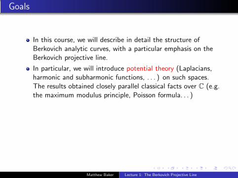
In this course, we will describe in detail the structure ofBerkovich analytic curves, with a particular emphasis on theBerkovich projective line.
In particular, we will introduce potential theory (Laplacians,harmonic and subharmonic functions, . . . ) on such spaces.The results obtained closely parallel classical facts over C (e.g.the maximum modulus principle, Poisson formula. . . )
The ultimate goal (which we will unfortunately not say muchabout) is to treat archimedean and non-archimedean analyticspaces in a unified way, and to make precise Arakelov’sanalogy between intersection theory on arithmetic surfacesand potential theory on Riemann surfaces.
Matthew Baker Lecture 1: The Berkovich Projective Line
Goals
In this course, we will describe in detail the structure ofBerkovich analytic curves, with a particular emphasis on theBerkovich projective line.
In particular, we will introduce potential theory (Laplacians,harmonic and subharmonic functions, . . . ) on such spaces.The results obtained closely parallel classical facts over C (e.g.the maximum modulus principle, Poisson formula. . . )
The ultimate goal (which we will unfortunately not say muchabout) is to treat archimedean and non-archimedean analyticspaces in a unified way, and to make precise Arakelov’sanalogy between intersection theory on arithmetic surfacesand potential theory on Riemann surfaces.
Matthew Baker Lecture 1: The Berkovich Projective Line

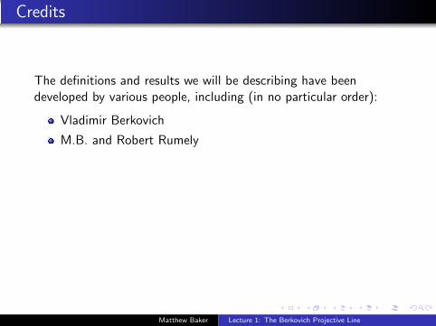
Credits
The definitions and results we will be describing have beendeveloped by various people, including (in no particular order):
Vladimir Berkovich
M.B. and Robert Rumely
Antoine Chambert-Loir
Amaury Thuillier
Juan Rivera-Letelier
Charles Favre and Mattias Jonsson
Ernst Kani
Matthew Baker Lecture 1: The Berkovich Projective Line
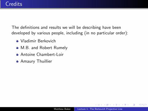
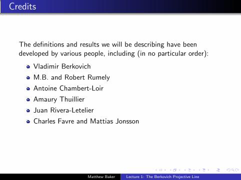
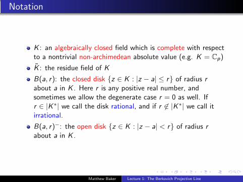
Notation
K : an algebraically closed field which is complete with respectto a nontrivial non-archimedean absolute value (e.g. K = Cp)
K : the residue field of K
B(a, r): the closed disk {z ∈ K : |z − a| ≤ r} of radius rabout a in K . Here r is any positive real number, andsometimes we allow the degenerate case r = 0 as well. Ifr ∈ |K ∗| we call the disk rational, and if r 6∈ |K ∗| we call itirrational.
B(a, r)−: the open disk {z ∈ K : |z − a| < r} of radius rabout a in K .
Matthew Baker Lecture 1: The Berkovich Projective Line

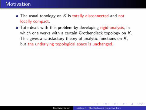
Motivation
The usual topology on K is totally disconnected and notlocally compact.
Tate dealt with this problem by developing rigid analysis, inwhich one works with a certain Grothendieck topology on K .This gives a satisfactory theory of analytic functions on K ,but the underlying topological space is unchanged.
The Berkovich affine line A1Berk over K is a locally compact,
Hausdorff, and uniquely path-connected topological spacewhich contains K as a dense subspace. The Berkovichprojective line P1
Berk is obtained by adjoining a point ∞ toA1
Berk.
One can view P1Berk as a profinite R-tree. This allows one to
define a Laplacian operator on P1Berk which comes from the
usual Laplacian on a finite graph. The tree structure alsoleads to a good theory of harmonic and subharmonic functionswhich closely parallels the classical theory over C.
Matthew Baker Lecture 1: The Berkovich Projective Line
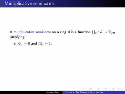
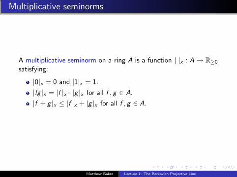
Multiplicative seminorms
A multiplicative seminorm on a ring A is a function | |x : A → R≥0
satisfying:
|0|x = 0 and |1|x = 1.
|fg |x = |f |x · |g |x for all f , g ∈ A.
|f + g |x ≤ |f |x + |g |x for all f , g ∈ A.
Matthew Baker Lecture 1: The Berkovich Projective Line

Multiplicative seminorms
A multiplicative seminorm on a ring A is a function | |x : A → R≥0
satisfying:
|0|x = 0 and |1|x = 1.
|fg |x = |f |x · |g |x for all f , g ∈ A.
|f + g |x ≤ |f |x + |g |x for all f , g ∈ A.
Matthew Baker Lecture 1: The Berkovich Projective Line
Multiplicative seminorms
A multiplicative seminorm on a ring A is a function | |x : A → R≥0
satisfying:
|0|x = 0 and |1|x = 1.
|fg |x = |f |x · |g |x for all f , g ∈ A.
|f + g |x ≤ |f |x + |g |x for all f , g ∈ A.
Matthew Baker Lecture 1: The Berkovich Projective Line

Multiplicative seminorms
A multiplicative seminorm on a ring A is a function | |x : A → R≥0
satisfying:
|0|x = 0 and |1|x = 1.
|fg |x = |f |x · |g |x for all f , g ∈ A.
|f + g |x ≤ |f |x + |g |x for all f , g ∈ A.
As a set, A1Berk,K consists of all multiplicative seminorms on the
polynomial ring K [T ] which extend the usual absolute value on K .
Matthew Baker Lecture 1: The Berkovich Projective Line
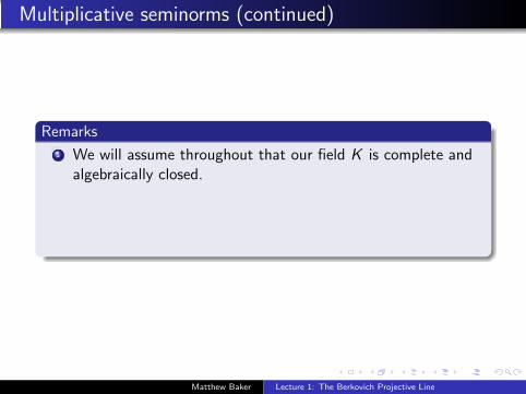
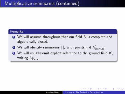
Multiplicative seminorms (continued)
Remarks
1 We will assume throughout that our field K is complete andalgebraically closed.
2 We will identify seminorms | |x with points x ∈ A1Berk,K .
3 We will usually omit explicit reference to the ground field K ,writing A1
Berk.
Matthew Baker Lecture 1: The Berkovich Projective Line

Topology on A1Berk
Definition
The topology on A1Berk,K is defined to be the weakest one for
which x 7→ |f |x is continuous for every f ∈ K [T ].
Matthew Baker Lecture 1: The Berkovich Projective Line

Topology on A1Berk
Definition
The topology on A1Berk,K is defined to be the weakest one for
which x 7→ |f |x is continuous for every f ∈ K [T ].
Explicitly, a fundamental system of open neighborhoods is given byopen sets of the form
{x ∈ A1Berk : αi < |fi |x < βi}
with f1, . . . , fm ∈ K [T ] and αi , βi ∈ R (i = 1, . . . ,m).
Matthew Baker Lecture 1: The Berkovich Projective Line

Motivation for the definition of A1Berk
The definition of A1Berk can be motivated by the following
observations:
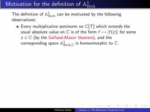
Every multiplicative seminorm on C[T ] which extends theusual absolute value on C is of the form f 7→ |f (z)| for somez ∈ C (by the Gelfand-Mazur theorem), and thecorresponding space A1
Berk,C is homeomorphic to C.When K is non-archimedean, there are many moremultiplicative seminorms on K [T ] than just the ones given byevaluation at a point of K .
Example
Fix a closed disk B(a, r) = {z ∈ K : |z − a| ≤ r} in K , and define| |B(a,r) by
|f |B(a,r) = supz∈B(a,r)
|f (z)|.
Then | |B(a,r) is a multiplicative seminorm on K [T ] (by Gauss’lemma).
Matthew Baker Lecture 1: The Berkovich Projective Line
Motivation for the definition of A1Berk
The definition of A1Berk can be motivated by the following
observations:
Every multiplicative seminorm on C[T ] which extends theusual absolute value on C is of the form f 7→ |f (z)| for somez ∈ C (by the Gelfand-Mazur theorem), and thecorresponding space A1
Berk,C is homeomorphic to C.
When K is non-archimedean, there are many moremultiplicative seminorms on K [T ] than just the ones given byevaluation at a point of K .
Example
Fix a closed disk B(a, r) = {z ∈ K : |z − a| ≤ r} in K , and define| |B(a,r) by
|f |B(a,r) = supz∈B(a,r)
|f (z)|.
Then | |B(a,r) is a multiplicative seminorm on K [T ] (by Gauss’lemma).
Matthew Baker Lecture 1: The Berkovich Projective Line

Motivation for the definition of A1Berk
The definition of A1Berk can be motivated by the following
observations:
Every multiplicative seminorm on C[T ] which extends theusual absolute value on C is of the form f 7→ |f (z)| for somez ∈ C (by the Gelfand-Mazur theorem), and thecorresponding space A1
Berk,C is homeomorphic to C.When K is non-archimedean, there are many moremultiplicative seminorms on K [T ] than just the ones given byevaluation at a point of K .
Example
Fix a closed disk B(a, r) = {z ∈ K : |z − a| ≤ r} in K , and define| |B(a,r) by
|f |B(a,r) = supz∈B(a,r)
|f (z)|.
Then | |B(a,r) is a multiplicative seminorm on K [T ] (by Gauss’lemma).
Matthew Baker Lecture 1: The Berkovich Projective Line
Embedding K into A1Berk,K
The set of all (possibly degenerate) disks B(a, r) thereforeembeds naturally into A1
Berk.
In particular, K embeds into A1Berk as the set of disks of
radius zero, and is dense in the Berkovich topology.
Similarly, P1(K ) can naturally be embedded as a dense subsetof P1
Berk.
Matthew Baker Lecture 1: The Berkovich Projective Line

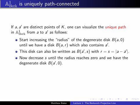
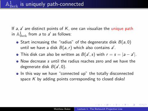
A1Berk is uniquely path-connected
If a, a′ are distinct points of K , one can visualize the unique pathin A1
Berk from a to a′ as follows:
Start increasing the “radius” of the degenerate disk B(a, 0)until we have a disk B(a, r) which also contains a′.
This disk can also be written as B(a′, s) with r = s = |a− a′|.Now decrease s until the radius reaches zero and we have thedegenerate disk B(a′, 0).
In this way we have “connected up” the totally disconnectedspace K by adding points corresponding to closed disks!
Matthew Baker Lecture 1: The Berkovich Projective Line

A1Berk is uniquely path-connected
If a, a′ are distinct points of K , one can visualize the unique pathin A1
Berk from a to a′ as follows:
Start increasing the “radius” of the degenerate disk B(a, 0)until we have a disk B(a, r) which also contains a′.
This disk can also be written as B(a′, s) with r = s = |a− a′|.
Now decrease s until the radius reaches zero and we have thedegenerate disk B(a′, 0).
In this way we have “connected up” the totally disconnectedspace K by adding points corresponding to closed disks!
Matthew Baker Lecture 1: The Berkovich Projective Line
A1Berk is uniquely path-connected
If a, a′ are distinct points of K , one can visualize the unique pathin A1
Berk from a to a′ as follows:
Start increasing the “radius” of the degenerate disk B(a, 0)until we have a disk B(a, r) which also contains a′.
This disk can also be written as B(a′, s) with r = s = |a− a′|.Now decrease s until the radius reaches zero and we have thedegenerate disk B(a′, 0).
In this way we have “connected up” the totally disconnectedspace K by adding points corresponding to closed disks!
Matthew Baker Lecture 1: The Berkovich Projective Line
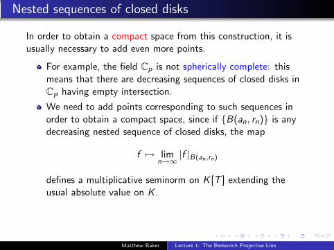
Nested sequences of closed disks
In order to obtain a compact space from this construction, it isusually necessary to add even more points.
For example, the field Cp is not spherically complete: thismeans that there are decreasing sequences of closed disks inCp having empty intersection.
We need to add points corresponding to such sequences inorder to obtain a compact space, since if {B(an, rn)} is anydecreasing nested sequence of closed disks, the map
f 7→ limn→∞
|f |B(an,rn)
defines a multiplicative seminorm on K [T ] extending theusual absolute value on K .
Two such sequences of disks with empty intersection definethe same seminorm if and only if the sequences are cofinal.
Matthew Baker Lecture 1: The Berkovich Projective Line

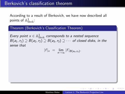
Berkovich’s classification theorem
According to a result of Berkovich, we have now described allpoints of A1
Berk:
Theorem (Berkovich’s Classification Theorem)
Every point x ∈ A1Berk corresponds to a nested sequence
B(a1, r1) ⊇ B(a2, r2) ⊇ B(a3, r3) ⊇ · · · of closed disks, in thesense that
|f |x = limn→∞
|f |B(an,rn).
Two such nested sequences define the same point of A1Berk if and
only if either:
1 each has a nonempty intersection, and their intersections arethe same; or
2 both have empty intersection, and the sequences are cofinal.
Matthew Baker Lecture 1: The Berkovich Projective Line
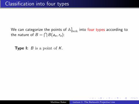
Classification into four types
We can categorize the points of A1Berk into four types according to
the nature of B =⋂
B(an, rn):
Type I: B is a point of K .
Type II: B is a closed disk with radius belonging to |K ∗|.Type III: B is an irrational disk with radius not belonging to |K ∗|.Type IV: B = ∅.
Matthew Baker Lecture 1: The Berkovich Projective Line

Classification into four types
We can categorize the points of A1Berk into four types according to
the nature of B =⋂
B(an, rn):
Type I: B is a point of K .
Type II: B is a closed disk with radius belonging to |K ∗|.
Type III: B is an irrational disk with radius not belonging to |K ∗|.Type IV: B = ∅.
Matthew Baker Lecture 1: The Berkovich Projective Line

Classification into four types
We can categorize the points of A1Berk into four types according to
the nature of B =⋂
B(an, rn):
Type I: B is a point of K .
Type II: B is a closed disk with radius belonging to |K ∗|.Type III: B is an irrational disk with radius not belonging to |K ∗|.
Type IV: B = ∅.
Matthew Baker Lecture 1: The Berkovich Projective Line

Classification into four types
We can categorize the points of A1Berk into four types according to
the nature of B =⋂
B(an, rn):
Type I: B is a point of K .
Type II: B is a closed disk with radius belonging to |K ∗|.Type III: B is an irrational disk with radius not belonging to |K ∗|.Type IV: B = ∅.
Matthew Baker Lecture 1: The Berkovich Projective Line

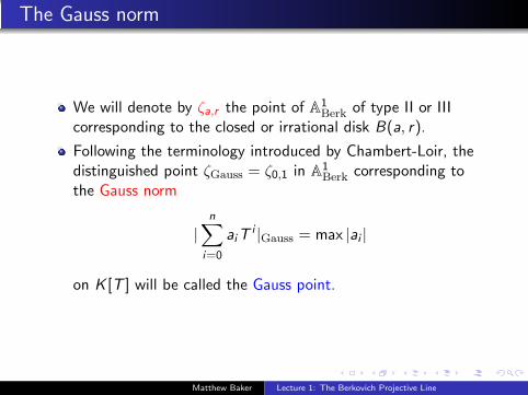
The Gauss norm
We will denote by ζa,r the point of A1Berk of type II or III
corresponding to the closed or irrational disk B(a, r).
Following the terminology introduced by Chambert-Loir, thedistinguished point ζGauss = ζ0,1 in A1
Berk corresponding tothe Gauss norm
|n∑
i=0
aiTi |Gauss = max |ai |
on K [T ] will be called the Gauss point.
Matthew Baker Lecture 1: The Berkovich Projective Line

A visual representation of P1Berk
r∞EEDDCCBBBBrAA( �������������������#�������
�����
(( �������
����
���
����
r
���
�����
������
#����
����
����
����
��
hh``` XXX PPPP
HHH
H
@@
@
AAAA
JJJ
SSSSSSSr b
...������EELLLSS
\\@@
@
HHQQZZcEEEE
DDDD
CCCC
BBBB
AA
hh``` XXX PPPP
HHH
H
QQZZcEEDDCCBBAA ����������(( �����
����
��
����
#s ζGauss
r 0
EEEEEEEEEEEr...b
(((( ��������
������������
����
���
���
����
��
��
��
��
��
��r
��� A
AAAA
EE��BBB�
���
�r XX...b
aaaaaaaaaa
HHHHH
HHH
HHH
HH
cccccccccccccr
@@@@
\\\\
JJJJ
AAAA
(( ��� �����
����
��
����
���
����
�
������#����
����
�����
�����
��EEEE
DDDD
CCCC
BBBB
AA
...b ���r A
AAr��r@r
(( ��� �����
����
��
����
���
����
�
������#����
����
����
����
��
EEDDCCBBAA
( ������������������#�������
�����
Matthew Baker Lecture 1: The Berkovich Projective Line

Alternate representation of P1Berk
Matthew Baker Lecture 1: The Berkovich Projective Line

Visualizing P1Berk
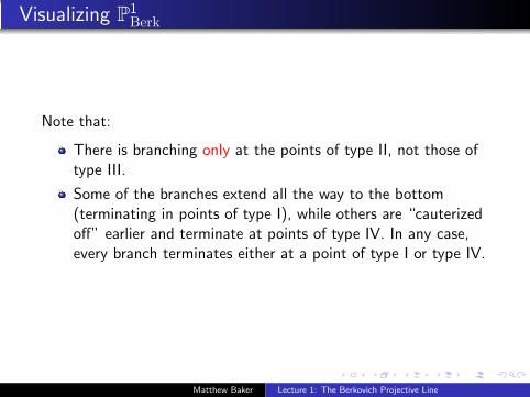
Note that:
There is branching only at the points of type II, not those oftype III.
Some of the branches extend all the way to the bottom(terminating in points of type I), while others are “cauterizedoff” earlier and terminate at points of type IV. In any case,every branch terminates either at a point of type I or type IV.
Matthew Baker Lecture 1: The Berkovich Projective Line
Visualizing P1Berk
Note that:
There is branching only at the points of type II, not those oftype III.
Some of the branches extend all the way to the bottom(terminating in points of type I), while others are “cauterizedoff” earlier and terminate at points of type IV. In any case,every branch terminates either at a point of type I or type IV.
Matthew Baker Lecture 1: The Berkovich Projective Line

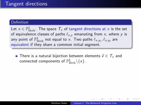
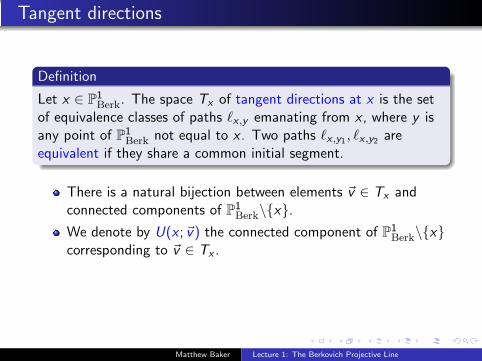
Tangent directions
Definition
Let x ∈ P1Berk. The space Tx of tangent directions at x is the set
of equivalence classes of paths `x ,y emanating from x , where y isany point of P1
Berk not equal to x . Two paths `x ,y1 , `x ,y2 areequivalent if they share a common initial segment.
There is a natural bijection between elements ~v ∈ Tx andconnected components of P1
Berk\{x}.We denote by U(x ;~v) the connected component of P1
Berk\{x}corresponding to ~v ∈ Tx .
The open sets U(x ;~v) for x ∈ P1Berk and ~v ∈ Tx generate the
topology on P1Berk.
Matthew Baker Lecture 1: The Berkovich Projective Line
Tangent directions
Definition
Let x ∈ P1Berk. The space Tx of tangent directions at x is the set
of equivalence classes of paths `x ,y emanating from x , where y isany point of P1
Berk not equal to x . Two paths `x ,y1 , `x ,y2 areequivalent if they share a common initial segment.
There is a natural bijection between elements ~v ∈ Tx andconnected components of P1
Berk\{x}.
We denote by U(x ;~v) the connected component of P1Berk\{x}
corresponding to ~v ∈ Tx .
The open sets U(x ;~v) for x ∈ P1Berk and ~v ∈ Tx generate the
topology on P1Berk.
Matthew Baker Lecture 1: The Berkovich Projective Line
Tangent directions
Definition
Let x ∈ P1Berk. The space Tx of tangent directions at x is the set
of equivalence classes of paths `x ,y emanating from x , where y isany point of P1
Berk not equal to x . Two paths `x ,y1 , `x ,y2 areequivalent if they share a common initial segment.
There is a natural bijection between elements ~v ∈ Tx andconnected components of P1
Berk\{x}.We denote by U(x ;~v) the connected component of P1
Berk\{x}corresponding to ~v ∈ Tx .
The open sets U(x ;~v) for x ∈ P1Berk and ~v ∈ Tx generate the
topology on P1Berk.
Matthew Baker Lecture 1: The Berkovich Projective Line
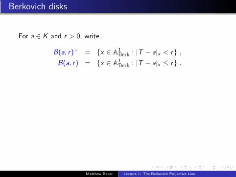
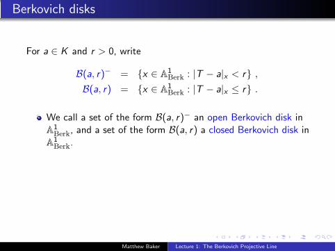
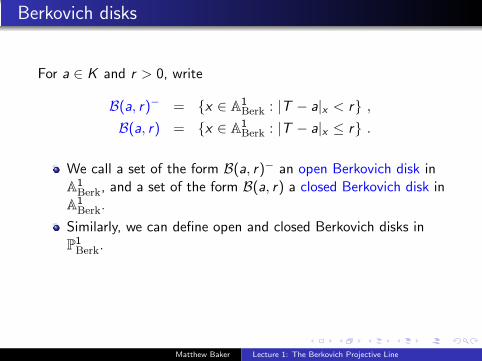
Berkovich disks
For a ∈ K and r > 0, write
B(a, r)− = {x ∈ A1Berk : |T − a|x < r} ,
B(a, r) = {x ∈ A1Berk : |T − a|x ≤ r} .
We call a set of the form B(a, r)− an open Berkovich disk inA1
Berk, and a set of the form B(a, r) a closed Berkovich disk inA1
Berk.
Similarly, we can define open and closed Berkovich disks inP1
Berk.
The intersection of a Berkovich open disk with P1(K ) is a(classical) open disk (and similarly for closed disks).
Matthew Baker Lecture 1: The Berkovich Projective Line

A Berkovich open disk
Matthew Baker Lecture 1: The Berkovich Projective Line
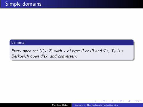
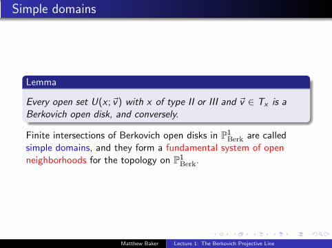
Simple domains
Lemma
Every open set U(x ;~v) with x of type II or III and ~v ∈ Tx is aBerkovich open disk, and conversely.
Matthew Baker Lecture 1: The Berkovich Projective Line
Simple domains
Lemma
Every open set U(x ;~v) with x of type II or III and ~v ∈ Tx is aBerkovich open disk, and conversely.
Finite intersections of Berkovich open disks in P1Berk are called
simple domains, and they form a fundamental system of openneighborhoods for the topology on P1
Berk.
Matthew Baker Lecture 1: The Berkovich Projective Line
Ends of a simple domain
A simple domain V in P1Berk has a finite set x1, . . . , xn of boundary
points, and a corresponding finite set ~v1, . . . , ~vn of ends, which arethe inward-pointing tangent directions:
Matthew Baker Lecture 1: The Berkovich Projective Line

Ends of a simple domain
A simple domain V in P1Berk has a finite set x1, . . . , xn of boundary
points, and a corresponding finite set ~v1, . . . , ~vn of ends, which arethe inward-pointing tangent directions:
Matthew Baker Lecture 1: The Berkovich Projective Line
Tangent directions at ζGauss
The tangent directions ~v ∈ TζGausscorrespond bijectively to
elements of P1(K ), the projective line over the residue field ofK .
Equivalently, elements of TζGausscorrespond to the open disks
of radius 1 contained in the closed unit disk B(0, 1), togetherwith the open disk
B(∞, 1)− := P1(K )\B(0, 1).
The correspondence between elements of TζGaussand open
disks is given explicitly by ~v 7→ U(ζGauss;~v).
Matthew Baker Lecture 1: The Berkovich Projective Line
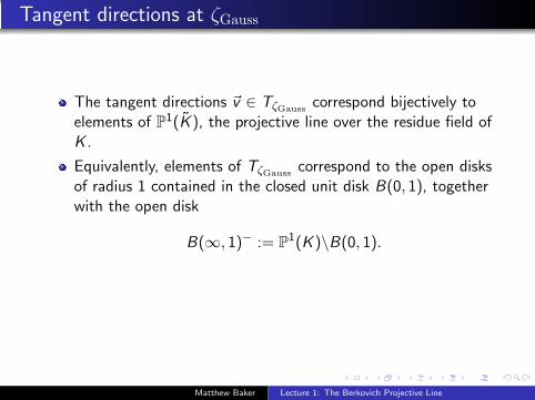
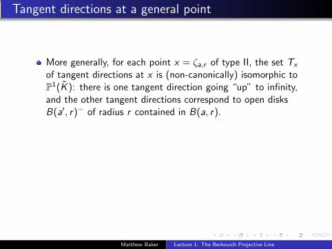
Tangent directions at a general point
More generally, for each point x = ζa,r of type II, the set Tx
of tangent directions at x is (non-canonically) isomorphic toP1(K ): there is one tangent direction going “up” to infinity,and the other tangent directions correspond to open disksB(a′, r)− of radius r contained in B(a, r).
For x ∈ P1Berk, we have:
|Tx | =
|P1(K )| x of type II2 x of type III1 x of type I or type IV.
Matthew Baker Lecture 1: The Berkovich Projective Line

Tangent directions at a general point
More generally, for each point x = ζa,r of type II, the set Tx
of tangent directions at x is (non-canonically) isomorphic toP1(K ): there is one tangent direction going “up” to infinity,and the other tangent directions correspond to open disksB(a′, r)− of radius r contained in B(a, r).
For x ∈ P1Berk, we have:
|Tx | =
|P1(K )| x of type II
2 x of type III1 x of type I or type IV.
Matthew Baker Lecture 1: The Berkovich Projective Line
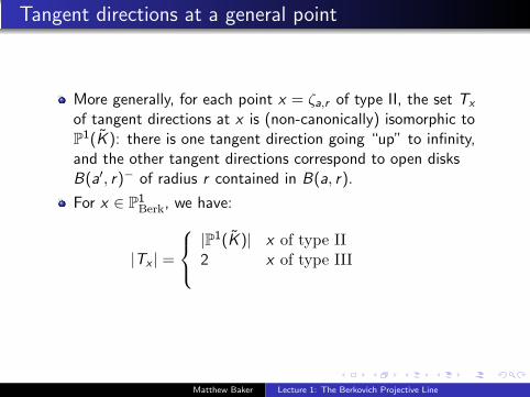
Tangent directions at a general point
More generally, for each point x = ζa,r of type II, the set Tx
of tangent directions at x is (non-canonically) isomorphic toP1(K ): there is one tangent direction going “up” to infinity,and the other tangent directions correspond to open disksB(a′, r)− of radius r contained in B(a, r).
For x ∈ P1Berk, we have:
|Tx | =
|P1(K )| x of type II2 x of type III
1 x of type I or type IV.
Matthew Baker Lecture 1: The Berkovich Projective Line
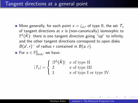
Tangent directions at a general point
More generally, for each point x = ζa,r of type II, the set Tx
of tangent directions at x is (non-canonically) isomorphic toP1(K ): there is one tangent direction going “up” to infinity,and the other tangent directions correspond to open disksB(a′, r)− of radius r contained in B(a, r).
For x ∈ P1Berk, we have:
|Tx | =
|P1(K )| x of type II2 x of type III1 x of type I or type IV.
Matthew Baker Lecture 1: The Berkovich Projective Line
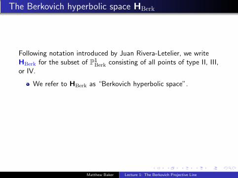
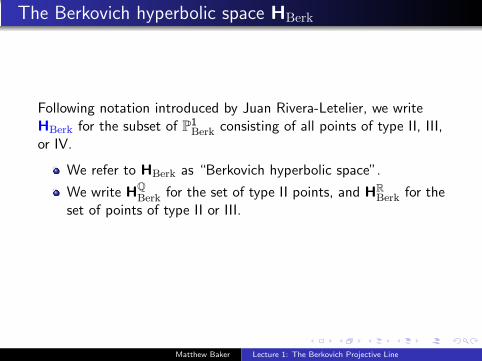
The Berkovich hyperbolic space HBerk
Following notation introduced by Juan Rivera-Letelier, we writeHBerk for the subset of P1
Berk consisting of all points of type II, III,or IV.
We refer to HBerk as “Berkovich hyperbolic space”.
We write HQBerk for the set of type II points, and HR
Berk for theset of points of type II or III.
The subset HQBerk is dense in P1
Berk.
Matthew Baker Lecture 1: The Berkovich Projective Line

The diameter function on A1Berk
Define the diameter function diam : A1Berk → R≥0 by setting
diam(x) = lim ri if x corresponds to the nested sequence{B(ai , ri )}.
If x ∈ HRBerk, then diam(x) is just the diameter (= radius) of
the corresponding closed disk.
In terms of multiplicative seminorms, we have
diam(x) = infa∈K
|T − a|x .
Because K is complete, if x is of type IV, then necessarilydiam(x) > 0. Thus diam(x) = 0 for x ∈ A1
Berk of type I, anddiam(x) > 0 for x ∈ HBerk.
Matthew Baker Lecture 1: The Berkovich Projective Line
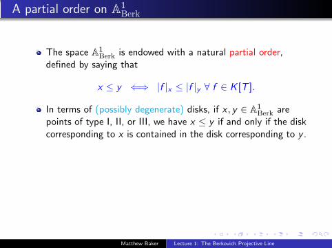
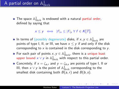
A partial order on A1Berk
The space A1Berk is endowed with a natural partial order,
defined by saying that
x ≤ y ⇐⇒ |f |x ≤ |f |y ∀ f ∈ K [T ].
In terms of (possibly degenerate) disks, if x , y ∈ A1Berk are
points of type I, II, or III, we have x ≤ y if and only if the diskcorresponding to x is contained in the disk corresponding to y .
For each pair of points x , y ∈ A1Berk, there is a unique least
upper bound x ∨ y in A1Berk with respect to this partial order.
Concretely, if x = ζa,r and y = ζb,s are points of type I, II orIII, then x ∨ y is the point of A1
Berk corresponding to thesmallest disk containing both B(a, r) and B(b, s).
Matthew Baker Lecture 1: The Berkovich Projective Line
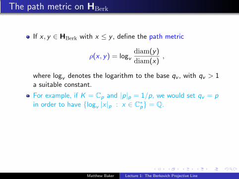
The path metric on HBerk
If x , y ∈ HBerk with x ≤ y , define the path metric
ρ(x , y) = logvdiam(y)
diam(x),
where logv denotes the logarithm to the base qv , with qv > 1a suitable constant.
For example, if K = Cp and |p|p = 1/p, we would set qv = pin order to have {logv |x |p : x ∈ C∗p} = Q.
More generally, for x , y ∈ HBerk arbitrary, we define
ρ(x , y) = ρ(x , x ∨ y) + ρ(y , x ∨ y) .
This gives an metric on HBerk.
Matthew Baker Lecture 1: The Berkovich Projective Line
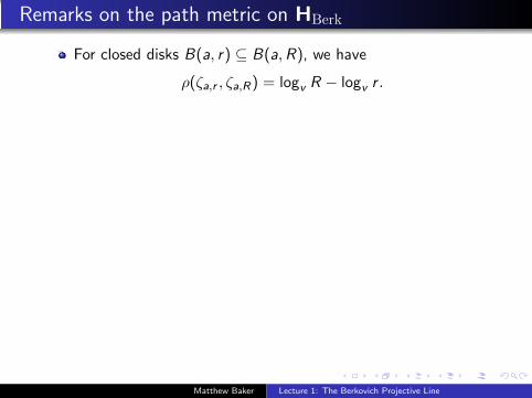
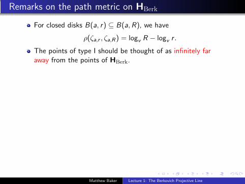
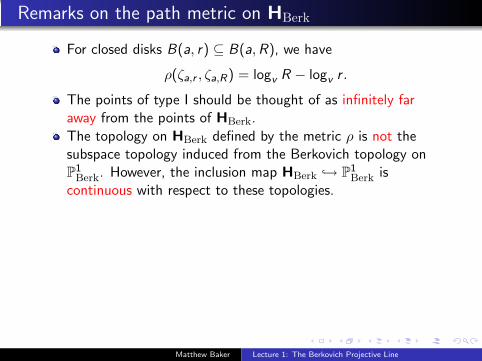
Remarks on the path metric on HBerk
For closed disks B(a, r) ⊆ B(a,R), we have
ρ(ζa,r , ζa,R) = logv R − logv r .
The points of type I should be thought of as infinitely faraway from the points of HBerk.
The topology on HBerk defined by the metric ρ is not thesubspace topology induced from the Berkovich topology onP1
Berk. However, the inclusion map HBerk ↪→ P1Berk is
continuous with respect to these topologies.
The group PGL(2,K ) of Mobius transformations actscontinuously on P1
Berk in a natural way compatible with theusual action on P1(K ), and this action preserves HBerk. Onecan show that PGL(2,K ) acts via isometries on HBerk, i.e.,
ρ(M(x),M(y)) = ρ(x , y)
for all x , y ∈ HBerk and all M ∈ PGL(2,K ). (This shows thatthe metric ρ is canonical).
Matthew Baker Lecture 1: The Berkovich Projective Line
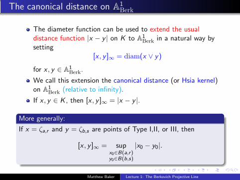
The canonical distance on A1Berk
The diameter function can be used to extend the usualdistance function |x − y | on K to A1
Berk in a natural way bysetting
[x , y ]∞ = diam(x ∨ y)
for x , y ∈ A1Berk.
We call this extension the canonical distance (or Hsia kernel)on A1
Berk (relative to infinity).
If x , y ∈ K , then [x , y ]∞ = |x − y |.
More generally:
If x = ζa,r and y = ζb,s are points of Type I,II, or III, then
[x , y ]∞ = supx0∈B(a,r)y0∈B(b,s)
|x0 − y0|.
Matthew Baker Lecture 1: The Berkovich Projective Line

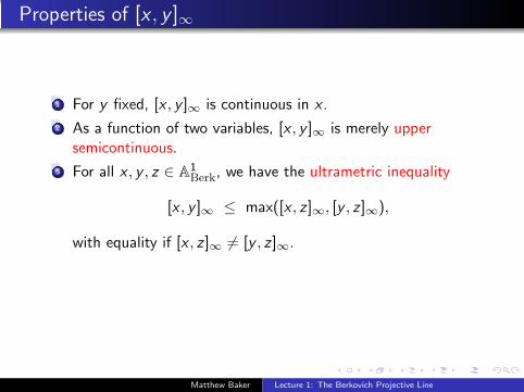
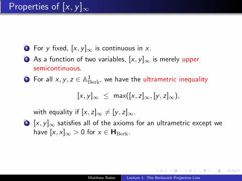
Properties of [x , y ]∞
1 For y fixed, [x , y ]∞ is continuous in x .
2 As a function of two variables, [x , y ]∞ is merely uppersemicontinuous.
3 For all x , y , z ∈ A1Berk, we have the ultrametric inequality
[x , y ]∞ ≤ max([x , z ]∞, [y , z ]∞),
with equality if [x , z ]∞ 6= [y , z ]∞.
4 [x , y ]∞ satisfies all of the axioms for an ultrametric except wehave [x , x ]∞ > 0 for x ∈ HBerk.
Matthew Baker Lecture 1: The Berkovich Projective Line


![Jascha Smacka - uni-regensburg.de...Berkovich spaces. In section 2 we will give a proof of this result (theorem 2.16), di ering from [JSS15] in the computation of the sheaves Lp X.](https://static.fdocuments.net/doc/165x107/5f700d4c70e89b61dc163405/jascha-smacka-uni-berkovich-spaces-in-section-2-we-will-give-a-proof-of.jpg)