POTENTIAL FLOWS OF VISCOUS AND VISCOELASTIC

FLUIDS

Daniel D. Joseph, Toshio Funada and Jing Wang

PREFACE

Potential flows of incompressible fluids are solutions of the Navier-Stokes equations which satisfy Laplace’s equa-tions. The Helmholtz decomposition says that every solution of the Navier-Stokes equations can be decomposedinto a rotational part and an irrotational part satisfying Laplace’s equation. The irrotational part is requiredto satisfy the boundary conditions; in general, the boundary conditions cannot be satisfied by the rotationalvelocity and they cannot be satisfied by the irrotational velocity; the rotational and irrotational velocities areboth required and they are tightly coupled at the boundary. For example, the no-slip condition for Stokes flowover a sphere cannot be satisfied by the rotational velocity; harmonic functions which satisfy Laplace’s equationsubject to a Robin boundary condition in which the irrotational normal and tangential velocities enter in equalproportions are required.

The literature which focuses on the computation of layers of vorticity in flows which are elsewhere irrotationaldescribes boundary layer solutions in the Helmholtz decomposed forms. These kind of solutions require smallviscosity and, in the case gas liquid flows are said to give rise to weak viscous damping. It is true that viscouseffects arising from these layers are weak but the main effects of viscosity in so many of these flows are purelyirrotational and they are not weak.

The theory of purely irrotational flows of a viscous fluid is an approximate theory which works well especiallyin gas-liquid flows of liquids of high viscosity, at low Reynolds numbers. The theory of purely irrotational flows ofa viscous fluid can be seen as a very successful competitor to the theory of purely irrotational flows of an inviscidfluid. We have come to regard every solution of free surface problems in an inviscid liquid as an opportunityfor problems in an inviscid liquid as an opportunity for a new paper. There are hundreds of such opportunitieswhich are still available.

The theory of irrotational flows of viscous and viscoelastic liquids which is developed here is embedded in avariety of fluid mechanics problems ranging from cavitation, capillary breakup and rupture, Rayleigh-Taylor andKelvin-Helmholtz instabilities, irrotational Faraday waves on a viscous fluid, flow induced structure of particlesin viscous and viscoelastic fluids, boundary layer theory for flow over rigid solids, rising bubbles and other topics.The theory of stability of free surface problems developed here is a great improvement of what was availablepreviously and could be used as supplemental text in courses on hydrodynamic stability.

We have tried to assemble here all the literature bearing on the irrotational flow of viscous liquids. For sure,it is not a large literature but it is likely that despite an honest effort it is probable that we missed some goodworks.

We are happy to acknowledge the contributions of persons who have helped us. Terrence Liao made veryimportant contributions to our early work on this subject in the early 1990’s. More recently, Juan Carlos Padrinojoined our group and has made truly outstanding contributions to problems described here. In a sense, JuanCarlos could be considered to be an author of this book and we are lucky that he came along. A subject likethis which develops an unconvential point of view is badly in need of friends and critics. We were lucky to findsuch a friend and critic in Professor G.I. Barenblatt who understands this subject and its importance. We arealso grateful to Professor K. Sreenivasan for his encouragement and help in recent years. The National ScienceFoundatiion has supported our work from the beginning.

We worked day and night on this research; Funada in his day and our night and Joseph and Wang in theirday and his night. The whole effort was a great pleasure.

– iii –

Contents

1 Introduction page 11.1 Irrotational flow, Laplace’s equation 21.2 Continuity equation, incompressible fluids, isochoric flow 31.3 Euler’s equations 31.4 Generation of vorticity in fluids governed by Euler’s equations 31.5 Perfect fluids, irrotational flow 41.6 Boundary conditions for irrotational flow 41.7 Streaming irrotational flow over a stationary sphere 5

2 Historical notes 72.1 Navier-Stokes equations 72.2 Stokes theory of potential flow of viscous fluid 82.3 The dissipation method 82.4 The distance a wave will travel before it decays by a certain amount 9

3 Boundary conditions for viscous fluids 10

4 Helmholtz decomposition coupling rotational to irrotational flow 124.1 Helmholtz decomposition 124.2 Navier-Stokes equations for the decomposition 134.3 Self-equilibration of the irrotational viscous stress 144.4 Dissipation function for the decomposed motion 154.5 Irrotational flow and boundary conditions 154.6 Examples from hydrodynamics 15

4.6.1 Poiseuille flow 154.6.2 Flow between rotating cylinders 164.6.3 Stokes flow around a sphere of radius a in a uniform stream U 164.6.4 Streaming motion past an ellipsoid (Lamb 1932, pp. 604-605) 174.6.5 Hadamard-Rybyshinsky solution for streaming flow past a liquid sphere 184.6.6 Axisymmetric steady flow around a spherical gas bubble at finite Reynolds numbers 184.6.7 Viscous decay of free gravity waves (Lamb 1932, § 349) 194.6.8 Oseen flow (Milne-Thomson, pp. 696-698, Lamb 1932, pp. 608-616) 194.6.9 Flows near internal stagnation points in viscous incompressible fluids 204.6.10 Hiemenz 1911 boundary layer solution for two-dimensional flow toward a “stagnation

point” at a rigid boundary 214.6.11 Jeffrey-Hamel flow in diverging and converging channels (Batchelor 1967, 294-302,

Landau and Lifshitz 1987, 76-81) 224.6.12 An irrotational Stokes flow 234.6.13 Lighthill’s approach 234.6.14 Conclusion 24

5 Harmonic functions which give rise to vorticity 25

6 Radial motions of a spherical gas bubble in a viscous liquid 28

– iv –

7 Rise velocity of a spherical cap bubble 307.1 Analysis 307.2 Experiments 337.3 Conclusions 36

8 Ellipsoidal model of the rise of a Taylor bubble in a round tube 378.1 Introduction 37

8.1.1 Unexplained and paradoxical features 388.1.2 Drainage 398.1.3 Brown’s 1965 analysis of drainage 398.1.4 Viscous potential flow 40

8.2 Ellipsoidal bubbles 418.2.1 Ovary ellipsoid 428.2.2 Planetary ellipsoid 448.2.3 Dimensionless rise velocity 45

8.3 Comparison of theory and experiment 468.4 Comparison of theory and correlations 488.5 Conclusion 49

9 Rayleigh-Taylor instability of viscous fluids 539.1 Acceleration 539.2 Simple thought experiments 549.3 Analysis 54

9.3.1 Linear theory of Chandrasekhar 559.3.2 Viscous potential flow 56

9.4 Comparison of theory and experiments 579.5 Comparison of the stability theory with the experiments on drop breakup 589.6 Comparison of the measured wavelength of corrugations on the drop surface with the

prediction of the stability theory 609.7 Fragmentation of Newtonian and viscoelastic drops 619.8 Modelling Rayleigh-Taylor instability of a sedimenting suspension of several thousand

circular particles in a direct numerical simulation 63

10 The force on a cylinder near a wall in viscous potential flows 6910.1 The flow due to the circulation about the cylinder 6910.2 The streaming flow past the cylinder near a wall 7110.3 The streaming flow past a cylinder with circulation near a wall 73

11 Kelvin-Helmholtz instability 7711.1 KH instability on an unbounded domain 7811.2 Maximum growth rate, Hadamard instability, neutral curves 78

11.2.1 Maximum growth rate 7911.2.2 Hadamard instability 7911.2.3 The regularization of Hadamard instability 7911.2.4 Neutral curves 79

11.3 KH instability in a channel 7911.3.1 Formulation of the problem 8011.3.2 Viscous potential flow analysis 8111.3.3 K-H Instability of inviscid fluid 8411.3.4 Dimensionless form of the dispersion equation 8511.3.5 The effect of liquid viscosity and surface tension on growth rates and neutral curves 8611.3.6 Comparison of theory and experiments in rectangular ducts 9211.3.7 Critical viscosity and density ratios 9311.3.8 Further comparisons with previous results 9411.3.9 Nonlinear effects 9511.3.10 Combinations of Rayleigh-Taylor and Kelvin-Helmholtz instabilities 96

– v –

12 Energy equation for irrotational theories of gas-liquid flow: viscous potential flow (VPF),viscous potential flow with pressure correction (VCVPF), dissipation method (DM) 9912.1 Viscous potential flow (VPF) 9912.2 Dissipation method according to Lamb 9912.3 Drag on a spherical gas bubble calculated from the viscous dissipation of an irrotational flow 10012.4 The idea of a pressure correction 10012.5 Energy equation for irrotational flow of a viscous fluid 10012.6 Viscous correction of viscous potential flow 102

13 Rising bubbles 10513.1 The dissipation approximation and viscous potential flow 105

13.1.1 Pressure correction formulas 10513.2 Rising spherical gas bubble 10613.3 Rising oblate ellipsoidal bubble (Moore 1965) ADD TO REFERENCE LIST 10613.4 A liquid drop rising in another liquid (Harper & Moore 1968) 10813.5 Purely irrotational analysis of the toroidal bubble in a viscous fluid 109

13.5.1 Prior work, experiments 10913.5.2 The energy equation 11013.5.3 The impulse equation 11313.5.4 Comparison of irrotational solutions for inviscid and viscous fluids 11413.5.5 Stability of the toroidal vortex 11713.5.6 Boundary integral study of vortex ring bubbles in a viscous liquid 11913.5.7 Irrotational motion of a massless cylinder under the combined action of Kutta-

Joukowski lift, acceleration of added mass and viscous drag 12013.6 The motion of a spherical gas bubble in viscous potential flow 12213.7 Steady motion of a deforming gas bubble in a viscous potential flow 12313.8 Dynamic simulations of the rise of many bubbles in a viscous potential flow 124

14 Purely irrotational theories of the effect of the viscosity on the decay of waves 12514.1 Decay of free gravity waves 125

14.1.1 Introduction 12514.1.2 Irrotational viscous corrections for the potential flow solution 12514.1.3 Relation between the pressure correction and Lamb’s exact solution 12714.1.4 Comparison of the decay rate and wave-velocity given by the exact solution, VPF

and VCVPF 12814.1.5 Why does the exact solution agree with VCVPF when k < kc and with VPF when

k > kc? 13014.1.6 Conclusion and discussion 13214.1.7 Quasipotential approximation – vorticity layers 133

14.2 Viscous decay of capillary waves on drops and bubbles 13414.2.1 Introduction 13514.2.2 VPF analysis of a single spherical drop immersed in another fluid 13614.2.3 VCVPF analysis of a single spherical drop immersed in another fluid 13914.2.4 Dissipation approximation (DM) 14214.2.5 Exact solution of the linearized free surface problem 14214.2.6 VPF and VCVPF analyses for waves acting on a plane interface considering surface

tension – comparison with Lamb’s solution 14414.2.7 Results and discussion 145

14.3 Irrotational dissipation of capillary-gravity waves 15014.3.1 Correction of the wave frequency assumed by Lamb 15014.3.2 Irrotational dissipation of nonlinear capillary-gravity waves 152

15 Irrotational Faraday waves on a viscous fluid 15415.1 Introduction 15515.2 Energy equation 15615.3 VPF & VCVPF 156

– vi –

15.3.1 Potential flow 15715.3.2 Amplitude equations for the elevation of the free surface 157

15.4 Dissipation method 16015.5 Stability analysis 16015.6 Rayleigh-Taylor instability and Faraday waves 16515.7 Comparison of purely irrotational solutions with exact solutions 16915.8 Bifurcation of Faraday waves in a nearly square container 17115.9 Conclusion 171

16 Stability of a liquid jet into incompressible gases and liquids 17216.1 Capillary instability of a liquid cylinder in another fluid 172

16.1.1 Introduction 17216.1.2 Linearized equations governing capillary instability 17316.1.3 Fully viscous flow analysis (Tomotika 1935) 17416.1.4 Viscous potential flow analysis (Funada and Joseph 2002) 17516.1.5 Pressure correction for viscous potential flow 17516.1.6 Comparison of growth rates 17816.1.7 Dissipation calculation for capillary instability 18016.1.8 Discussion of the pressure corrections at the interface of two viscous fluids 18516.1.9 Capillary instability when one fluid is a dynamically inactive gas 18816.1.10 Conclusions 190

16.2 Stability of a liquid jet into incompressible gases: temporal, convective and absolute instability19116.2.1 Introduction 19116.2.2 Problem formulation 19216.2.3 Dispersion relation 19316.2.4 Temporal instability 19416.2.5 Numerical results of temporal instability 20416.2.6 Spatial, absolute and convective instability 20616.2.7 Algebraic equations at a singular point 20816.2.8 Subcritical, critical and supercritical singular points 21016.2.9 Inviscid jet in inviscid fluid (R →∞, m = 0) 21616.2.10 Exact solution; comparison with previous results 21716.2.11 Conclusions 219

16.3 Viscous potential flow of the Kelvin-Helmholtz instability of a cylindrical jet of one fluidinto the same fluid 22016.3.1 Mathematical formulation 22016.3.2 Normal modes; dispersion relation 22016.3.3 Growth rates and frequencies 22116.3.4 Hadamard instabilities for piecewise discontinuous profiles 222

17 Stress induced cavitation 22417.1 Theory of stress induced cavitation 224

17.1.1 Mathematical formulation 22517.1.2 Cavitation threshold 227

17.2 Viscous potential flow analysis of stress induced cavitation in an aperture flow 22817.2.1 Analysis of stress induced cavitation 22917.2.2 Stream function, potential function and velocity 23117.2.3 Cavitation threshold 23117.2.4 Conclusions 23317.2.5 Navier-Stokes simulation 234

17.3 Streaming motion past a sphere 23817.3.1 Irrotational flow of a viscous fluid 23817.3.2 An analysis for maximum K 242

17.4 Symmetric model of capillary collapse and rupture 24417.4.1 Introduction 245

– vii –

17.4.2 Analysis 24617.4.3 Conclusions and discussion 25017.4.4 Appendix 252

18 Viscous effects of the irrotational flow outside boundary layers on rigid solids 25618.1 Extra drag due to viscous dissipation of the irrotational flow outside the boundary layer 257

18.1.1 Pressure corrections for the drag on a circular gas bubble 25718.1.2 A rotating cylinder in a uniform stream 26018.1.3 The additional drag on an airfoil by dissipation method 26718.1.4 Discussion and conclusion 270

18.2 Glauert’s solution of the boundary layer on a rapidly rotating clylinder in a uniform streamrevisited 27118.2.1 Introduction 27218.2.2 Unapproximated governing equations 27518.2.3 Boundary layer approximation and Glauert’s equations 27518.2.4 Decomposition of the velocity and pressure field 27618.2.5 Solution of the boundary layer flow 27718.2.6 Higher-order boundary layer theory 28418.2.7 Discussion and conclusion 287

18.3 Numerical study of the steady state uniform flow past a rotating cylinder 28918.3.1 Introduction 28918.3.2 Numerical features 29118.3.3 Results and dicussion 29318.3.4 Concluding remarks 299

19 Irrotational flows which satisfy the compressible Navier-Sokes equations. 31019.1 Acoustics 31019.2 Liquid jet in a high Mach number air stream 31219.3 Liquid jet in a high Mach number air stream 313

19.3.1 Introduction 31319.3.2 Basic partial differential equations 31419.3.3 Cylindrical liquid jet in a compressible gas 31519.3.4 Basic isentropic relations 31519.3.5 Linear stability of the cylindrical liquid jet in a compressible gas; dispersion equation 31619.3.6 Stability problem in dimensionless form 31719.3.7 Inviscid potential flow (IPF) 32019.3.8 Growth rate parameters as a function of M for different viscosities 32019.3.9 Azimuthal periodicity of the most dangerous disturbance 32519.3.10 Variation of the growth rate parameters with the Weber number 32719.3.11 Convective/absolute (C/A) instability 32719.3.12 Conclusions 328

20 Irrotational flows of viscoelastic fluids 33020.1 Oldroyd B model 33020.2 Asymptotic form of the constitutive equations 331

20.2.1 Retarded motion expansion for the UCM model 33120.2.2 The expanded UCM model in potential flow 33120.2.3 Potential flow past a sphere calculated using the expanded UCM model 332

20.3 Second order fluids 33320.4 Purely irrotational flows 33420.5 Purely irrotational flows of a second order fluid 33420.6 Reversal of the sign of the normal stress at a point of stagnation 33520.7 Fluid forces near stagnation points on solid bodies 336

20.7.1 Turning couples on long bodies 33620.7.2 Particle-particle interactions 33620.7.3 Sphere-wall interactions 337

– viii –

20.7.4 Flow induced microstructure. 33820.8 Potential flow over a sphere for a second order fluid 33920.9 Potential flow over an ellipse 340

20.9.1 Normal stress at the surface of the ellipse 34120.9.2 The effects of the Reynolds number 34220.9.3 The effects of −α1/

(ρa2

)343

20.9.4 The effects of the aspect ratio 34420.10 The moment on the ellipse 34520.11 The reversal of the sign of the normal stress at stagnation points 34720.12 Flow past a flat plate 34720.13 Flow past a circular cylinder with circulation 34820.14 Potential flow of a second-order fluid over a tri-axial ellipsoid 34820.15 The lift, drag and torque on an airfoil in foam modeled by the potential flow of a second-order

fluid 34920.15.1 Introduction 34920.15.2 Numerical method 35020.15.3 Results 352

21 Purely irrotational theories of stability of viscoelastic fluids 35621.1 Rayleigh-Taylor instability of viscoelastic drops at high Weber numbers 356

21.1.1 Introduction 35621.1.2 Experiments 35721.1.3 Theory 35921.1.4 Comparison of theory and experiment 366

21.2 Purely irrotational theories of the effects of viscosity and viscoelasticity on capillaryinstability of a liquid cylinder 36821.2.1 Introduction 36921.2.2 Linear stability equations and the exact solution (Tomotika 1935) 37021.2.3 Viscoelastic potential flow (VPF) 37121.2.4 Dissipation and the formulation for the additional pressure contribution 37221.2.5 The additional pressure contribution for capillary instability 37321.2.6 Comparison of the growth rate 37421.2.7 Comparison of the stream function 37521.2.8 Discussion 379

21.3 Steady motion of a deforming gas bubble in a viscous potential flow 383

22 Numerical methods for irrotational flows of viscous fluid 38522.1 Perturbation methods 38522.2 Boundary integral methods for inviscid potential flow 38522.3 Boundary integral methods for viscous potential flow 38722.4 Boundary integral methods for effects of viscosity and surface tension on steep surface waves 387

Appendix 1 Equations of motion and strain rates for rotational and irrotational flow in carte-sian, cylindrical and spherical coordinates 393

Appendix 2 Tests of BibTeX 397References 402List of Illustrations 411List of Tables 427

– ix –

1

Introduction

The theory of potential flow is a topic in the study of fluid mechanics and is also a topic in mathematics.The mathematical theory treats properties of vector fields generated by gradients of a potential. The curl of agradient vanishes. The local rotation of a vector field is proportional to its curl so that potential flows do notrotate as they deform. Potential flows are irrotational.

The mathematical theory of potentials goes back to the 18th century (see Kellogg 1929). This elegant theoryhas given rise to jewels of mathematical analysis, such as the theory of a complex variable. It is a well formed or“mature” theory meaning that the best research results have already been obtained. We are not going to add tothe mathematical theory; our contributions are to the fluid mechanics theory focusing on effects of viscosity andviscoelasticity. Two centuries of research have focused exclusively on the motions of inviscid fluids. Among the131,000,000 hits which come up under “potential flows” on Google search are mathematical studies of potentialfunctions and studies of inviscid fluids. These studies can be extended to viscous fluids at small cost and greatprofit.

The fluid mechanics theory of potential flow goes back to Euler (1761) (see Truesdell 1954 § 36). The concept ofviscosity was not known in Euler’s time. The fluids he studied are driven by pressures and not by viscous stresses.The effects of viscous stresses were introduced by Navier (1822) and Stokes (1845). Stokes (1851) consideredpotential flow of a viscous fluid in an approximate sense but most later authors restrict their attention to“potential flow of an inviscid fluid.” All the books on fluid mechanics and all courses in fluid mechanics havechapters on “potential flow of inviscid fluids” and none on the “potential flow of a viscous fluid.”

An authoritative and readable exposition of irrotational flow theory and its applications can be found inChapter 6 of the book on fluid dynamics by Batchelor (1967). He speaks of the role of the theory of flow of aninviscid fluid. He says

In this and the following chapter, various aspects of the flow of a fluid regarded as entirely inviscid (and incompressible)will be considered. The results presented are significant only inasmuch as they represent an approximation to the flowof a real fluid at large Reynolds number, and the limitations of each result must be regarded as important as the resultitself.

In this book we consider irrotational flows of a viscous fluid. We are of the opinion that when consideringirrotational solutions of the Navier-Stokes equations it is never necessary and typically not useful to put theviscosity to zero. This observation runs counter to the idea frequently expressed that potential flow is a topicwhich is useful only for inviscid fluids; many people think that the notion of a viscous potential flow is anoxymoron. Incorrect statements like “. . . irrotational flow implies inviscid flow but not the other way around”can be found in popular textbooks.

Irrotational flows of a viscous fluid scale with the Reynolds number as do rotational solutions of the Navier-Stokes equations generally. The solutions of the Navier-Stokes equations, rotational and irrotational, are thoughtto become independent of the Reynolds number at large Reynolds numbers. Unlike the theory of irrotationalflows of inviscid fluids, the theory of irrotational flow of a viscous fluid can be considered as a description offlow at a finite Reynolds number.

Most of the classical theorems reviewed in Chapter 6 of Batchelor’s 1967 book do not require that the fluidbe inviscid. These theorems are as true for viscous potential flow as they are for inviscid potential flow. Kelvin’sminimum energy theorem holds for the irrotational flow of a viscous fluid. The theory of the acceleration reactionleads to the concept of added mass; it follows from the analysis of unsteady irrotational flow. The theory appliesto viscous and inviscid fluids alike.

It can be said that every theorem about potential flow of inviscid incompressible fluids applies equally to

1

viscous fluids in regions of irrotational flow. Jeffreys (1928) derived an equation (his (20)) which replaces thecirculation theorem of classical (inviscid) hydrodynamics. When the fluid is homogeneous, Jeffreys’ equationmay be written as

dC

dt= −µ

ρ

∮curlω · dl, (1.0.1)

where

ω = curlu and C (t) =∮

u · dl

is the circulation round a closed material curve drawn in the fluid. This equation shows that

. . . the initial value of dC/dt around a contour in a fluid originally moving irrotationally is zero, whether or not there isa moving solid within the contour. This at once provides an explain of the equality of the circulation about an aeroplaneand that about the vortex left behind when it starts; for the circulation about a large contour that has never been cutby the moving solid or its wake remains zero, and therefore the circulations about contours obtained by subdividing itmust also add up to zero. It also indicates why the motion is in general nearly irrotational except close to a solid of tofluid that has pass near one.

Saint-Venant (1869) interpreted the result of Lagrange 1781 about the invariance of circulation dC/dt = 0to mean that

vorticity cannot be generated in the interior of a viscous incompressible fluid, subject to conservative extraneous force,but is necessarily diffused inward from the boundaries.

The circulation formula (1.0.1) is an important result in the theory of irrotational flows of a viscous fluid. Aparticle which is initially irrotational will remain irrotational in motions which do not enter into the vorticallayers at the boundary.

1.1 Irrotational flow, Laplace’s equation

A potential flow is a velocity field u (φ) given by the gradient of a potential φ

u (φ) = ∇φ. (1.1.1)

Potential flows have a zero curl

curlu = curl∇φ = 0. (1.1.2)

Fields that are curl free, satisfying (1.1.2), are called irrotational.Vector fields satisfying the equation

divu = 0 (1.1.3)

are said to be solenoidal. Solenoidal flows which are irrotational are harmonic; the potential satisfies Laplace’sequation

divu (φ) = div∇φ = ∇2φ = 0. (1.1.4)

The theory of irrotational flow needed in this book is given in many books; for example, Lamb (1932), Milne-Thomson (1960), Batchelor (1967), and Landau and Lifshitz (1987). No-slip cannot be enforced in irrotationoalflow. However, eliminating all the irrotational effects of viscosity by putting µ = 0 to reconcile our desire tosatisfy no-slip at the cost of real physics is like throwing out the baby with the bath water. This said, the readercan rely on the book by Batchelor and others for the results we need in our study of irrotational flow of viscousfluids.

2

1.2 Continuity equation, incompressible fluids, isochoric flow

The equation governing the evolution of the density ρ

dρ

dt+ ρdivu = 0, (1.2.1)

dρ

dt=

∂ρ

∂t+ (u · ∇) ρ

is called the continuity equation. It guarantees that the mass of a fluid element is conserved.If the fluid is incompressible, then ρ is constant, and divu = 0. Flows of compressible fluids for which

divu = 0 are called isochoric. Low Mach number flows are nearly isochoric. Incompressible and isochoric flowsare solenoidal.

1.3 Euler’s equations

Euler’s equations of motion

ρdu

dt= −∇p + ρg, (1.3.1)

du

dt=

∂u

∂t+ (u · ∇) u

where g is a body force per unit mass. If ρ is constant and g = ∇G has a force potential, then

−∇p + ρg = −∇p (1.3.2)

where p = p− ρG can be called the pressure head. If g is gravity, then

G = g · x.

To simplify the writing of equations we will put the body force to zero except in cases where it is important.If the fluid is compressible, then an additional relation, from thermodynamics, relating p to ρ will be required.Such a relation can be found for isentropic flow, or isothermal flow of a perfect gas. In such a system there arefive unknowns p, ρ and u and five equations.

The effects of viscosity are absent in Euler’s equations of motion. The effects of viscous stresses are absent inEuler’s theory; the flows are driven by pressure. The Navier-Stokes equations reduce to Euler’s equations whenthe fluid is inviscid.

1.4 Generation of vorticity in fluids governed by Euler’s equations

The Euler equation (1.3.1) may be written as

∂u

∂t− u× ω +

12∇|u|2 = g − ∇p

ρ(1.4.1)

where we have used the vector identity

(u · ∇) u =12∇|u|2 − u× ω (1.4.2)

and

ω = ω [u] = curlu.

The vorticity equation can be obtained by forming the curl of (1.4.1)

∂ω

∂t+ u · ∇ω = ω · ∇u− curl

∇p

ρ+ curlg. (1.4.3)

If curl∇p

ρ= ∇×

(1ρp′(ρ)∇ρ

)= 0 and curlg = 0, then ω [u] = 0; curlg = 0 if g is given by a potential g = ∇G.

Flows for which curl∇p

ρ= 0 are said to be barotropic. Barotropic flows governed by Euler’s equation with

conservative body forces g = ∇G, cannot generate vorticity. If the fluid is incompressible, then the flow isbarotropic.

3

1.5 Perfect fluids, irrotational flow

Inviscid fluids which are also incompressible are called “perfect” or “ideal.” Perfect fluids satisfy Euler’s equa-tions. Perfect fluids with conservative body forces give rise to a Bernoulli equation

∇

ρ

[∂φ

∂t+

12|∇φ|2

]+ p−G

= 0

ρ

[∂φ

∂t+

12|∇φ|2

]+ p−G = f (t) . (1.5.1)

We may absorb the function f (t) into the potential φ = φ +∫ t

f (t) dt without changing the velocity

∇φ = ∇[φ +

∫ t

f (t) dt

]= ∇φ = u. (1.5.2)

The Bernoulli equation relates p and φ before any problem is solved; actually curlu = 0 is a constraint onsolutions. The velocity u is determined by φ satisfying ∇2φ = 0 and the boundary conditions.

1.6 Boundary conditions for irrotational flow

Irrotational flows have a potential and if the flow is solenoidal the potential φ is harmonic, ∇2φ = 0. This bookreveals the essential role of harmonic functions in the flow of incompressible viscous and viscoelastic fluids.All the books on partial differential equations have sections devoted to the mathematical analysis of Laplaceequations. Laplace’s equation may be solved for prescribed data on the boundary of the flow region includinginfinity for flows on unbounded domains. It can be solved for Dirichlet data in which values of φ are prescribedon the boundary or for Neuman data in which the normal component of ∇φ is prescribed on the boundary.Almost any combination of Dirichlet and Neuman data all over the boundary will lead to unique solutions ofLaplace’s equation.

It is important that unique solutions can be obtained when only one condition is required for φ at eachpoint on the boundary. The problem is over determined when two conditions are prescribed. We can solve theproblem when Dirichlet conditions are prescribed or when Neuman conditions are prescribed but not when bothare prescribed. In the case in which Neuman conditions are prescribed over the whole the boundary the solutionis unique up to the addition of any constant. If the boundary condition is not specified at each point on theboundary, then the problem may be not over-determined when two conditions are prescribed.

This point can be forcefully made in the frame of fluid dynamics. Consider, for example, the irrotationalstreaming flow over a body. The velocity U at infinity in the direction x is given by the potential φ = U · x.The tangential component of velocity on the boundary S of the body is given by

uS = eS · u = eS · ∇φ (1.6.1)

where eS is a unit lying entirely in S. The normal component of velocity on S is given by

un = n · u = n · ∇φ (1.6.2)

where n is the unit normal pointing from body to fluid.Laplace’s equation for streaming flow can be solved if

eS · ∇φ is prescribed on S,

say,

eS · ∇φ = 0 on S (1.6.3)

or if

n · ∇φ is prescribed on S,

say,

n · ∇φ = 0 on S. (1.6.4)

It cannot be solved if eS · ∇φ = 0 and n · ∇φ = 0 are simultaneously required on S.

4

Ux

r

θ

Fig. 1.1. Axisymmetric flow over a sphere of radius a. The flow depends on the radius r and the polar angle θ.

The prescription of the tangential velocity on S is a Dirichlet condition. If φ is prescribed on S the tangentialderivatives can be computed, only one prescription of the tangential velocity is allowed because prescribing twoindependent tangential derivatives is not compatible with one φ.

The no-slip condition of viscous fluid mechanics requires that

uS = 0 and un = 0. (1.6.5)

simultaneously on S. This condition cannot be satisfied by potential flow. In fact, these conditions cannot besatisfied by solutions of Euler’s equations even when they are not irrotational.

The point of view which has been universally adopted by researchers and students of fluid mechanics forseveral centuries is that the normal component should be enforced so that the fluid does not penetrate thesolid. The fluid must then slip at the boundary because there is no other choice. To reconcile this with no-slip,researchers put the viscosity to zero. The resolution of these difficulties lies in the fact that real flows have a nonzero rotational velocity at boundaries generated by the no-slip condition. The no-slip condition usually cannotbe satisfied by the rotational velocity alone; the irrotational velocity is also needed (see Chapter 4).

1.7 Streaming irrotational flow over a stationary sphere

A flow of speed U in the direction x = r cos θ streams past a sphere of radius a (see figure 1.1). A solution φ ofLaplace’s equation ∇2φ = 0 in spherical polar coordinates is

φ = Ur cos θ +c

r2cos θ. (1.7.1)

The normal and tangential components of the velocity at r = a are, respectively

∂φ

∂r= U cos θ − 2c

a3cos θ, (1.7.2)

1a

∂φ

∂θ= −U sin θ − c

a3sin θ. (1.7.3)

If the normal velocity is prescribed to be zero on the sphere, then c = Ua3/2 and

φ1 = U

(r +

a3

2r2

)cos θ. (1.7.4)

The corresponding tangential velocity is −3U sin θ/2. If the tangential velocity is prescribed to be zero on thesphere, then c = −Ua3 and

φ2 = U

(r − a3

r2

)cos θ. (1.7.5)

The corresponding normal velocity is 3U cos θ.The preceding analysis and uniqueness of solutions of Laplace’s equation shows that the solution φ1 with a

zero normal velocity may be obtained by prescribing the non zero function − 32U sin θ for the tangential velocity.

The solution φ2 with a zero tangential velocity may be obtained by prescribing the non zero function 3U cos θ

for the normal velocity.More complicated conditions for harmonic solutions on rigid bodies are encountered in exact solutions of the

5

Navier-Stokes equations in which irrotational and rotational flows are tightly coupled at the boundary. Theboundary conditions cannot be satisfied without irrotational flow and they cannot be satisfied by irrotationalflow only (cf. equation (4.6.6)).

6

2

Historical notes

Potential flows of viscous fluids are an unconventional topic with a niche history assembled in a recent reviewarticle Joseph 2006.

2.1 Navier-Stokes equations

The history of Navier-Stokes equations begins with the 1822 memoir of Navier who derived equations forhomogeneous incompressible fluids from a molecular argument. Using similar arguments, Poisson (1829) derivedthe equations for a compressible fluid. The continuum derivation of the Navier-Stokes equation is due to SaintVenant (1843) and Stokes (1845). In his (1847) paper Stokes wrote that

Let P1, P2, P3 be the three normal, and T1, T2, T3 the three tangential pressures in the direction of three rectangularplanes parallel to the co-ordinate planes, and let D be the symbol of differentiation with respect to t when the particle andnot the point of space remains the same. Then the general equations applicable to a heterogeneous fluid (the equations(10) of my former (1845) paper), are

ρ

„Du

Dt−X

«+

dP1

dx+

dT3

dy+

dT2

dz= 0, (132)

with the two other equations which may be written down from symmetry. The pressures P1, T1, etc. are given by theequations

P1 = p− 2µ

„du

dx− δ

«, T1 = −µ

„dv

dz+

dw

dy

«, (133)

and four other similar equations. In these equations

3δ =du

dx+

dv

dy+

dw

dz. (134)

The equations written by Stokes in his 1845 paper are the same ones we use today:

ρ

(du

dt−X

)= divT, (2.1.1)

where X is presumably a body force, which was not specified by Stokes, and

T =(−p− 2

3µ divu

)1 + 2µD[u], (2.1.2)

du

dt=

∂u

∂t+ (u · ∇) u, (2.1.3)

D[u] =12

[∇u +∇uT], (2.1.4)

dρ

dt+ ρ divu = 0. (2.1.5)

Stokes assumed that the bulk viscosity −23µ divu is selected so that the deviatoric part of T vanishes and

traceT = −3p.Inviscid fluids are fluids with zero viscosity. Viscous effects on the motion of fluids were not understood

before the notion of viscosity was introduced by Navier in 1822. Perfect fluids, following the usage of Stokes

7

and other 19th century English mathematicians, are inviscid fluids which are also incompressible. Statementslike Truesdell’s 1954,

In 1781 Lagrange presented his celebrated velocity-potential theorem: if a velocity potential exists at one time in a motionof an inviscid incompressible fluid, subject to conservative extraneous force, it exists at all past and future times.

though perfectly correct, could not have been asserted by Lagrange, since the concept of an inviscid fluid wasnot available in 1781.

2.2 Stokes theory of potential flow of viscous fluid

The theory of potential flow of a viscous fluid was introduced by Stokes in 1851. All of his work on this topic isframed in terms of the effects of viscosity on the attenuation of small amplitude waves on a liquid-gas surface.Everything he said about this problem is cited below. The problem treated by Stokes was solved exactly,usingthe linearized Navier-Stokes equations, without assuming potential flow, by Lamb 1932.

Stokes discussion is divided into three parts discussed in §51, 52, 53.(1) The dissipation method in which the decay of the energy of the wave is computed from the viscous

dissipation integral where the dissipation is evaluated on potential flow (§51).(2) The observation that potential flows satisfy the Navier-Stokes equations together with the notion that

certain viscous stresses must be applied at the gas-liquid surface to maintain the wave in permanent form (§52).(3) The observation that if the viscous stresses required to maintain the irrotational motion are relaxed, the

work of those stresses is supplied at the expense of the energy of the irrotational flow (§53).Lighthill 1978 discussed Stokes’ ideas but he did not contribute more to the theory of irrotational motions of

a viscous fluid. On page 234 he notes that

“Stokes ingenious idea was to recognize that the average value of the rate of working given by sinusoidal waves of wavenumber

2µˆ(∂φ/∂x) ∂2φ/∂x∂z + (∂φ/∂z) ∂2φ/∂z2˜

z=0

which is required to maintain the unattenuated irrotational motions of sinusoidal waves must exactly balance the rateat which the same waves when propagating freely would lose energy by internal dissipation.”

Lamb 1932 gave an exact solution of the problem considered by Stokes in which vorticity and boundarylayers are not neglected. Wang-Joseph 2006 (JFM 557, 145-165) did purely irrotational theories of Stokesproblem which are in good agreement with Lamb’s exact solution.

2.3 The dissipation method51. By means of the expression given in Art. 49, for the loss of vis viva due to internal friction, we may readily obtaina very approximate solution of the problem: To determine the rate at which the motion subsides, in consequence ofinternal friction, in the case of a series of oscillatory waves propagated along the surface of a liquid. Let the verticalplane of xy be parallel to the plane of motion, and let y be measured vertically downwards from the mean surface; andfor simplicity’s sake suppose the depth of the fluid very great compared with the length of a wave, and the motion sosmall that the square of the velocity may be neglected. In the case of motion which we are considering, udx + vdy is anexact differential dφ when friction is neglected, and

φ = cε−my sin (mx− nt) , (140)

where c, m, n are three constants, of which the last two are connected by a relation which it is not necessary to writedown. We may continue to employ this equation as a near approximation when friction is taken into account, providedwe suppose c, instead of being constant, to be parameter which varies slowly with the time. Let V be the vis viva of agiven portion of the fluid at the end of the time t, then

V = ρc2m2

ZZZε−2mydxdydz. (141)

But by means of the expression given in Art.49, we get for the loss of vis viva during the time dt, observing that in thepresent case µ is constant, w = 0, δ = 0, and udx + vdy = dφ, where φ is independent of z,

4µdt

ZZZ („d2φ

dx2

«2

+

„d2φ

dy2

«2

+ 2

„d2φ

dxdy

«2)

dxdydz

8

which becomes, on substituting for φ its value,

8µc2m4dt

ZZZε−2mydxdydz.

But we get from (141) for the decrement of vis viva of the same mass arising from the variation of the parameter c

−2ρm2cdc

dtdt

ZZZε−2mydxdydz.

Equating the two expressions for the decrement of vis viva, putting for m its value 2πλ−1, where λ is the length of awave, replacing µ by µ′ρ, integrating, and supposing c0 to be the initial value of c, we get

c = c0ε− 16π2µ′t

λ2 .∗It will presently appear that the value of

√µ′ for water is about 0.0564, an inch and a second being the units of space

and time. Suppose first that λ is two inches, and t ten seconds. Then 16π2µ′tλ−2 = 1.256, and c: c0:: 1 : 0.2848, so thatthe height of the waves, which varies as c, is only about a quarter of what it was. Accordingly, the ripples excited on asmall pool by a puff of wind rapidly subside when the exciting cause ceases to act.

Now suppose that λ is to fathoms or 2880 inches, and that t is 86400 seconds or a whole day. In this case 16π2µ′tλ−2

is equal to only 0.005232, so that by the end of an entire day, in which time waves of this length would travel 574English miles, the height would be diminished by little more than the one two hundredth part in consequence of friction.Accordingly, the long swells of the ocean are but little allayed by friction, and at last break on some shore situated atthe distance of perhaps hundreds of miles from the region where they were first excited.

* In a footnote on page 624, Lamb notes that “Through an oversight in the original calculation the valueλ2/16π2ν was too small by one half.” The value 16 should be 8.

2.4 The distance a wave will travel before it decays by a certain amount

The observations made by Stokes about the distance a wave will travel before its amplitude decays by a givenamount, point the way to a useful frame for the analysis of the effects of viscosity on wave propagation. Manystudies of nonlinear irrotational waves can be found in the literature but the only study of the effects of viscosityon the decay of these waves known to us is due to M. Longuet-Higgins (1997) who used the dissipation method todetermine the decay due to viscosity of irrotational steep capillary-gravity waves in deep water. He finds that thelimiting rate of decay for small amplitude solitary waves are twice those for linear periodic waves computed bythe dissipation method. The dissipation of very steep waves can be more than ten times more than linear wavesdue to the sharply increased curvature in wave troughs. He assumes that that the nonlinear wave maintains itssteady form while decaying under the action of viscosity. The wave shape could change radically from its steadyshape in very steep waves.

Stokes (1880) studied the motion of nonlinear irrotational gravity waves in two dimensions which are prop-agated with a constant velocity, and without change of form. This analysis led Stokes 1880 to the celebratedmaximum wave whose asymptotic form gives rise to a pointed crest of angle 120. The effects of viscosity onsuch extreme waves has not been studied but they may be studied by the dissipation method or same potentialflow theory used by Stokes (1851) for inviscid fluids with the caveat that the normal stress condition that p

vanish on the free surface be replaced by the condition that

p + 2µ∂un/∂n = 0

on the free surface with normal n where the velocity component un = ∂φ/∂n is given by the potential.

9

3

Boundary conditions for viscous fluids

Boundary conditions for incompressible viscous fluids cannot usually be satisfied without contributions frompotential flows (Joseph, Renardy 1991, § 1.2 (d)).

(1) No-slip conditions are required at the boundary S of a rigid solid:

u = U for x ∈ S, (3.0.1)

where U is the velocity of the solid.(2) At the interface S between two fluids, the fluid velocities are continuous, the shear stress is continuous

and the stress is balanced by surface tension.Now we shall express the condition just mentioned with equations. Let the position of the surface S as it

moves through the surface be F (x (t) , t) = 0 where x (t) ∈ S for all t and x (t) ∈ uS is the velocity of pointsof S. Since F = 0 is an identity in t, we have

dF

dt=

∂F

∂t+ uS · ∇F = 0; (3.0.2)

in fact dmF/dtm = 0 for all m. Now, the normal n to S (figure 3.1) is n = ∇F/ |∇F |; hence

uS · ∇F = (n · uS) |∇F | . (3.0.3)

The tangential component of uS is irrelevant and

n · uS = n · u, (3.0.4)

where u is the velocity of a material point on x ∈ S.We now set a convention for jumps in the value of variables as we cross S at x. Define

[[•]] = (•)1 − (•)2 ,

where the subscript (•)1 means to evaluate (•) at x in the fluid 1; likewise for 2.Combining (3.0.2), (3.0.3), and (3.0.4), we get the kinematic equation for the evolution of F

dF

dt=

∂F

∂t+ u · ∇F = 0. (3.0.5)

Since[[

∂F

∂t

]]= 0, we have

[[u · n]] = [[u]] · n = 0. (3.0.6)

Fig. 3.1. Interface S between two fluids.

10

The normal component of velocity is continuous. If the tangential component of velocity is also continuousacross S, we have

n× [[u]] = 0 x ∈ S. (3.0.7)

Turning now to the stress

T = −p1 + 2µD[u], (3.0.8)

Tij = −pδij + µ

(∂ui

∂xj+

∂uj

∂xi

),

we express the continuity of the shear stress as

eS · [[2µD[u]]] · n = 0, (3.0.9)

where eS is a unit vector tangent to S; eS · ∇F = 0.The condition that the jump in the normal component of the stress is balanced by a surface tension force

may be expressed as

n · [[T]] · n = − [[p]] + 2n · [[µD[u]]] · n = 2Hγ −∇Sγ, (3.0.10)

where H is the mean curvature

2H =1

R1+

1R2

(3.0.11)

and R1 and R2 are principal radii of curvature. The surface gradient is

∇S = ∇− n (n · ∇) . (3.0.12)

The curvature 2H is determined by the surface gradient of the normal (see Joseph and Renardy, 1991)

2H = ∇S · n. (3.0.13)

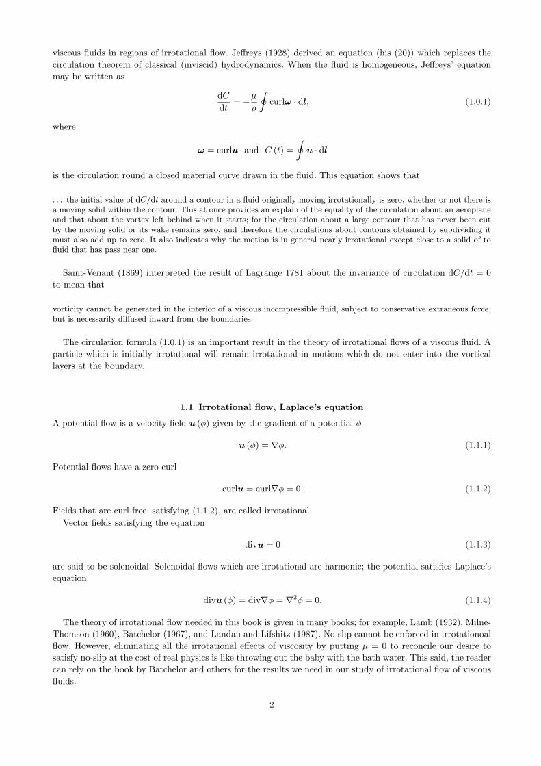
(3) Free surfaces. Free surfaces are two fluid interfaces for which one fluid is a dynamically inactive gas. Thedensity of the gas is usually much less than the density of the liquid and the viscosity of the gas is usuallymuch less than the viscosity of the liquid. In some cases we can put the viscosity and density of the gas tozero; then we have a liquid-vacuum interface. This procedure works well for problems of capillary instabilityand Rayleigh-Taylor instability. However, for Kelvin-Helmholtz instabilities the kinematic viscosity ν = µ/ρ isimportant and ν for the liquid and gas are of comparable magnitude. The dynamic participation of the ambientis necessary for Kelvin-Helmholtz instability.

For free surface problems with a dynamically inactive ambient, no condition on the tangential velocity of theinterface is required; the shear stress vanishes

2µeS ·D [u] · n = 0, x ∈ S (3.0.14)

and the normal stress balance is

− p + 2µn ·D [u] · n = 2Hγ −∇Sγ (3.0.15)

Sometimes the sign of the mean curvature is ambiguous (we could have assigned n from 2 to 1). A quick wayto determine the sign is to look at the terms

− p = 2(

1R1

+1

R2

)γ

making sure the pressure is higher inside the equivalent sphere.Summarizing, the main equations on S are (3.0.5), (3.0.6), (3.0.7), (3.0.9), (3.0.10), (3.0.14), and (3.0.15).

These equations are written for Cartesian, cylindrical, and spherical polar coordinates in Appendix A.

11

4

Helmholtz decomposition coupling rotationalto irrotational flow

In this chapter we present the form of the Navier-Stokes equations implied by the Helmholtz decomposition inwhich the relation of the irrotational and rotational velocity fields is made explicit. The idea of self-equilibrationof irrotational viscous stresses is introduced. The decomposition is constructed by first selecting the irrotationalflow compatible with the flow boundaries and other prescribed conditions. The rotational component of velocityis then the difference between the solution of the Navier-Stokes equations and the selected irrotational flow. Tosatisfy the boundary conditions the irrotational field is required and it depends on the viscosity. Five unknownfields are determined by the decomposed form of the Navier-Stokes equations for an incompressible fluid; therotational component of velocity, the pressure and the harmonic potential. These five fields may be readilyidentified in analytic solutions available in the literature. It is clear from these exact solutions that potentialflow of a viscous fluid is required to satisfy prescribed conditions, like the no-slip condition at the boundary of asolid or continuity conditions across a two-fluid boundary. The decomposed form of the Navier-Stokes equationsmay be suitable for boundary layers because the target irrotational flow which is expected to appear in the limit,say at large Reynolds numbers, is an explicit to-be-determined field. It can be said that equations governing theHelmholtz decomposition describe the modification of irrotational flow due to vorticity but the analysis showsthe two fields are coupled and cannot be completely determined independently.

4.1 Helmholtz decomposition

The Helmholtz decomposition theorem says that every smooth vector field u, defined everywhere in space andvanishing at infinity together with its first derivatives can be decomposed into a rotational part v and anirrotational part ∇φ,

u = v +∇φ, (4.1.1)

where

divu = divv +∇2φ, (4.1.2)

curlu = curlv. (4.1.3)

This decomposition leads to the theory of the vector potential which is not followed here. The decompositionis unique on unbounded domains without boundaries and explicit formulas for the scalar and vector potentialsare well known. A framework for embedding the study of potential flows of viscous fluids, in which no specialflow assumptions are made, is suggested by this decomposition (Joseph 2006a, c). If the fields are solenoidal,then

divu = divv = 0 and ∇2φ = 0. (4.1.4)

Since φ is harmonic, we have from (4.1.1) and (4.1.4) that

∇2u = ∇2v. (4.1.5)

The irrotational part of u is on the null space of the Laplacian but in special cases, like plane shear flow,∇2v = 0 but curlv 6= 0.

Unique decompositions are generated by solutions of the Navier-Stokes equation (4.2.1) in decomposed form(4.2.2) where the irrotational flows satisfy (4.1.1), (4.1.3), (4.1.4) and (4.1.5) and certain boundary conditions.

12

The boundary conditions for the irrotational flows have a heavy weight in all this. Simple examples of uniquedecomposition, taken from hydrodynamics, will be presented later.

The decomposition of the velocity into rotational and irrotational parts holds at each and every point andvaries from point to point in the flow domain. Various possibilities for the balance of these parts at a fixed pointand the distribution of these balances from point to point can be considered.

(i) The flow is purely irrotational or purely rotational. These two possibilities do occur as approximationsbut are not typical.

(ii) Typically the flow is mixed with rotational and irrotational components at each point.

4.2 Navier-Stokes equations for the decomposition

To study solutions of the Navier-Stokes equations, it is convenient to express the Navier-Stokes equations foran incompressible fluid

ρdu

dt= −∇p + µ∇2u, (4.2.1)

in terms of the rotational and irrotational fields implied by the Helmholtz decomposition

ρ∂v

∂t+∇

ρ∂φ

∂t+

ρ

2|∇φ|2 + p

+ ρdiv [v ⊗∇φ +∇φ⊗ v + v ⊗ v] = µ∇2v, (4.2.2)

or

ρ∂vi

∂t+

∂

∂xi

ρ∂φ

∂t+

ρ

2|∇φ|2 + p

+ ρ

∂

∂xj

(vj

∂φ

∂xi+ vi

∂φ

∂xj+ vivj

)= µ∇2vi,

satisfying (4.1.4).To solve this problem in a domain Ω, say, when the velocity u = V is prescribed on ∂Ω, we would need to

compute a solenoidal field v satisfying (4.2.2) and a harmonic function φ satisfying ∇2φ = 0 such that

v +∇φ = V on ∂Ω.

Since this system of five equations in five unknowns is just the decomposed form of the four equations in fourunknowns which define the Navier-Stokes system for u, it ought to be possible to study this problem usingexactly the same mathematical tools that are used to study the Navier-Stokes equations.

In the Navier-Stokes theory for incompressible fluid the solutions are decomposed into a space of gradientsand its complement which is a space of solenoidal vectors. The gradient space is not, in general, solenoidalbecause the pressure is not solenoidal. If it were solenoidal, then ∇2p = 0, but ∇2p = −divρu · ∇u satisfiesPoisson’s equation.

It is not true that only the pressure is found on the gradient space. Indeed equation (4.2.2) gives rise to aPoisson’s equation for the Bernoulli function, not just the pressure:

∇2

[ρ∂φ

∂t+

ρ

2|∇φ|2 + p

]= −ρ

∂2

∂xi∂xj

(vj

∂φ

∂xi+ vi

∂φ

∂xj+ vivj

).

In fact, there may be hidden irrotational terms on the right hand side of this equation.The boundary condition for solutions of (4.2.1) is

u− a = 0 on ∂Ω,

where a is solenoidal field, a = V on ∂Ω. Hence,

v − a +∇φ = 0 (4.2.3)

The decomposition depends on the selection of the harmonic function φ; the traditional boundary condition

n · a = n · ∇φ on ∂Ω (4.2.4)

together with a Dirichlet condition at infinity when the region of flow is unbounded and a prescription of thevalue of the circulation in doubly connected regions, gives rise to a unique φ. Then the rotational flow mustsatisfy

v · n = 0 and es · (v − a) + es · ∇φ = 0 (4.2.5)

13

on ∂Ω. The v determined in this way is rotational and satisfies (4.1.3). However, v may contain other harmoniccomponents.

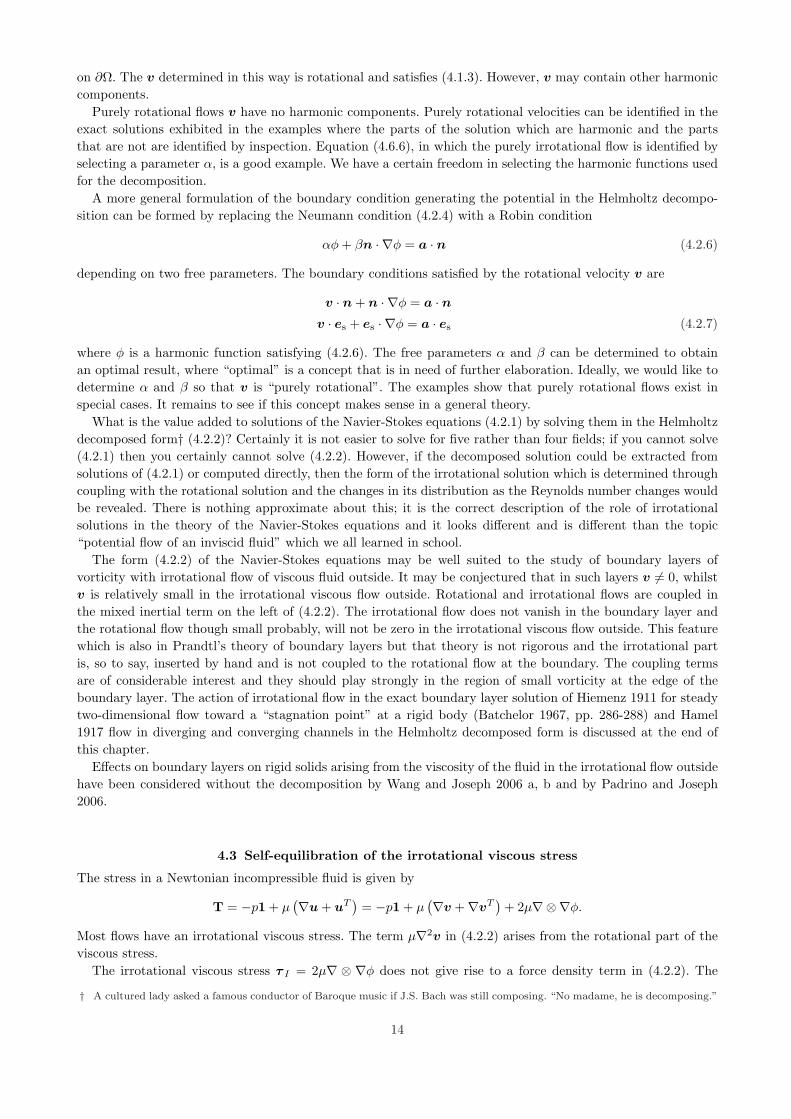
Purely rotational flows v have no harmonic components. Purely rotational velocities can be identified in theexact solutions exhibited in the examples where the parts of the solution which are harmonic and the partsthat are not are identified by inspection. Equation (4.6.6), in which the purely irrotational flow is identified byselecting a parameter α, is a good example. We have a certain freedom in selecting the harmonic functions usedfor the decomposition.

A more general formulation of the boundary condition generating the potential in the Helmholtz decompo-sition can be formed by replacing the Neumann condition (4.2.4) with a Robin condition

αφ + βn · ∇φ = a · n (4.2.6)

depending on two free parameters. The boundary conditions satisfied by the rotational velocity v are

v · n + n · ∇φ = a · nv · es + es · ∇φ = a · es (4.2.7)

where φ is a harmonic function satisfying (4.2.6). The free parameters α and β can be determined to obtainan optimal result, where “optimal” is a concept that is in need of further elaboration. Ideally, we would like todetermine α and β so that v is “purely rotational”. The examples show that purely rotational flows exist inspecial cases. It remains to see if this concept makes sense in a general theory.

What is the value added to solutions of the Navier-Stokes equations (4.2.1) by solving them in the Helmholtzdecomposed form† (4.2.2)? Certainly it is not easier to solve for five rather than four fields; if you cannot solve(4.2.1) then you certainly cannot solve (4.2.2). However, if the decomposed solution could be extracted fromsolutions of (4.2.1) or computed directly, then the form of the irrotational solution which is determined throughcoupling with the rotational solution and the changes in its distribution as the Reynolds number changes wouldbe revealed. There is nothing approximate about this; it is the correct description of the role of irrotationalsolutions in the theory of the Navier-Stokes equations and it looks different and is different than the topic“potential flow of an inviscid fluid” which we all learned in school.

The form (4.2.2) of the Navier-Stokes equations may be well suited to the study of boundary layers ofvorticity with irrotational flow of viscous fluid outside. It may be conjectured that in such layers v 6= 0, whilstv is relatively small in the irrotational viscous flow outside. Rotational and irrotational flows are coupled inthe mixed inertial term on the left of (4.2.2). The irrotational flow does not vanish in the boundary layer andthe rotational flow though small probably, will not be zero in the irrotational viscous flow outside. This featurewhich is also in Prandtl’s theory of boundary layers but that theory is not rigorous and the irrotational partis, so to say, inserted by hand and is not coupled to the rotational flow at the boundary. The coupling termsare of considerable interest and they should play strongly in the region of small vorticity at the edge of theboundary layer. The action of irrotational flow in the exact boundary layer solution of Hiemenz 1911 for steadytwo-dimensional flow toward a “stagnation point” at a rigid body (Batchelor 1967, pp. 286-288) and Hamel1917 flow in diverging and converging channels in the Helmholtz decomposed form is discussed at the end ofthis chapter.

Effects on boundary layers on rigid solids arising from the viscosity of the fluid in the irrotational flow outsidehave been considered without the decomposition by Wang and Joseph 2006 a, b and by Padrino and Joseph2006.

4.3 Self-equilibration of the irrotational viscous stress

The stress in a Newtonian incompressible fluid is given by

T = −p1 + µ(∇u + uT

)= −p1 + µ

(∇v +∇vT)

+ 2µ∇⊗∇φ.

Most flows have an irrotational viscous stress. The term µ∇2v in (4.2.2) arises from the rotational part of theviscous stress.

The irrotational viscous stress τ I = 2µ∇ ⊗ ∇φ does not give rise to a force density term in (4.2.2). The

† A cultured lady asked a famous conductor of Baroque music if J.S. Bach was still composing. “No madame, he is decomposing.”

14

divergence of τ I vanishes on each and every point in the domain V of flow. Even though an irrotational viscousstress exists, it does not produce a net force to drive motions. Moreover,

∫divτ IdV =

∮n · τ IdS = 0. (4.3.1)

The traction vectors n · τ I have no net resultant on each and every closed surface in the domain V of flow. Wesay that the irrotational viscous stresses, which do not drive motions, are self-equilibrated. Irrotational viscousstresses are not equilibrated at boundaries and they may produce forces there.

4.4 Dissipation function for the decomposed motion

The dissipation function evaluated on the decomposed field (4.1.1) sorts out into rotational, mixed and irrota-tional terms given by

Φ =∫

V

2µDijDijdV

=∫

2µDij [v]Dij [v] dV + 4µ

∫Dij [v]

∂2φ

∂xi∂xjdV + 2µ

∫∂2φ

∂xi∂xj

∂2φ

∂xi∂xjdV. (4.4.1)

Most flows have an irrotational viscous dissipation. In regions V ′ where v is small, we have approximately that

T = −p1 + 2µ∇⊗∇φ, (4.4.2)

and

Φ = 2µ

∫

V ′

∂2φ

∂xi∂xj

∂2φ

∂xi∂xjdV. (4.4.3)

Equation (4.4.3) has been widely used to study viscous effects in irrotational flows since Stokes 1851.

4.5 Irrotational flow and boundary conditions

How is the irrotational flow determined? It frequently happens that the rotational motion cannot satisfy theboundary conditions; this well known problem is associated with difficulties in forming boundary conditions forthe vorticity. The potential φ is a harmonic function which can be selected so that the values of the sum of therotational and irrotational fields can be chosen to balance prescribed conditions at the boundary. The allowedirrotational fields can be selected from harmonic functions that enter into the purely irrotational solution ofthe same problem on the same domain. A very important property of potential flow arises from the fact thatirrotational viscous stresses do not give rise to irrotational viscous forces in the equations (4.2.2) of motion.The interior values of the rotational velocity are coupled to the irrotational motion through Bernoulli termsevaluated on the potential and inertial terms which couple the irrotational and rotational fields. The dependenceof the irrotational field on viscosity can be generated by the boundary conditions.

4.6 Examples from hydrodynamics

4.6.1 Poiseuille flow

A simple example which serves as a paradigm for the relation of the irrotational and rotational components ofvelocity in all the solutions of the Navier-Stokes equations, is plane Poiseuille flow

u =[−P ′

2µ

(b2 − y2

), 0, 0

],

curlu =[0, 0, −P ′y

µ

],

v =[

P ′

2µy2, 0, 0

],

∇φ =[−P ′

2µb2, 0, 0

].

(4.6.1)

15

The rotational flow is a constrained field and cannot satisfy the no-slip boundary condition. To satisfy theno-slip condition we add the irrotational flow

∂φ

∂x= −P ′

2µb2.

The irrotational component is for uniform and unidirectional flow chosen so that u = 0 at the boundary.

4.6.2 Flow between rotating cylinders

u = eθu (r),

u = eθΩaa at r = a,

u = eθΩab at r = b,

u (r) = Ar +B

r,

A = −a2Ωa − b2Ωb

b2 − a2,

B =(Ωa − Ωb) a2b2

b2 − a2,

v = eθAr,

1r

∂φ

∂θ=

B

r.

(4.6.2)

The irrotational flow with v = 0 is an exact solution of the Navier-Stokes equations with no-slip at boundaries.

4.6.3 Stokes flow around a sphere of radius a in a uniform stream U

This axisymmetric flow, described with spherical polar coordinates (r, θ, ϕ), is independent of ϕ. The velocitycomponents can be obtained from a stream function ψ (r, θ) such that

u = (ur, uθ) =1

r sin θ

(1r

∂ψ

∂θ, −∂ψ

∂r

). (4.6.3)

The stream function can be divided into rotational and irrotational parts

ψ = ψv + ψp, ∇2ψp = 0, (4.6.4)

where ψp is the conjugate harmonic function. The potential φ corresponding to ψp is given by

φ =(− A

2r2+ Cr

)2 cos θ

where the parameters A and C are selected to satisfy the boundary conditions on u.The Helmholtz decomposition of the solution of the problem of slow streaming motion over a stationary

16

sphere is given by

u = (ur, uθ) =(

vr +∂φ

∂r, vθ +

1r

∂φ

∂θ

),

ur = U

[1− 3a

2r+

12

(a

r

)3]

cos θ,

uθ = −U

[1− 3a

4r− 1

4

(a

r

)3]

sin θ,

curlu = U

[0, 0, − 3a

2r2sin θ

],

vr = −32

a

rU cos θ,

vθ =34

a

rU sin θ,

φ = U

[r − 1

4a3

r2

]cos θ,

p− p∞ = −32

a

r2µU cos θ.

(4.6.5)

The potential for flow over a sphere is

φ = U

[r − α

4a3

r2

]cos θ. (4.6.6)

The normal component of velocity vanishes when α = −2 and the tangential component vanishes when α = 4. Inthe present case, to satisfy the no-slip condition, we take α = 1. Both the rotational and irrotational componentsof velocity are required to satisfy the no-slip condition.

4.6.4 Streaming motion past an ellipsoid (Lamb 1932, pp. 604-605)

The problem of the steady translation of an ellipsoid in a viscous liquid was solved by Lamb 1932 in terms ofthe gravitational-potential Ω of the solid and another harmonic function χ corresponding to the case in which∇2χ = 0, finite at infinity with χ = 1 for the internal space. Citing Lamb

If the fluid be streaming past the ellipsoid, regarded as fixed, with the general velocity U in the direction of x, we assume

u = A∂2Ω

∂x2+ B

„x

∂χ

∂x− χ

«+ U, v = A

∂2Ω

∂x∂y+ Bx

∂χ

∂y, w = A

∂2Ω

∂x∂z+ Bx

∂χ

∂z.

These satisfy the equation of continuity, in virtue of the relations

∇2Ω = 0, ∇2χ = 0;

and they evidently make u = U , v = 0, w = 0 at infinity. Again, they make

∇2u = 2B∂2χ

∂x2, ∇2v = 2B

∂2χ

∂x∂y, ∇2w = 2B

∂2χ

∂x∂z.

We note next that ∇2v = ∇2u; the irrotational part of u is on the null space of the Laplacian. It followsthat the rotational velocity is associated with χ and is given by the terms proportional to B. The irrotationalvelocity is given by

∇φ = ∇(

A∂Ω∂x

).

The vorticity is given by

ω = −ey

(2B

∂χ

∂z

)+ ez

(2B

∂χ

∂y

).

17

4.6.5 Hadamard-Rybyshinsky solution for streaming flow past a liquid sphere

As in the flow around a solid sphere, this problem is posed in spherical coordinates with a stream function andpotential function related by (4.6.3), (4.6.4) and (4.6.5). The stream function is given by

ψ = f (r) sin2 θ, (4.6.7)

f (r) =A

r+ Br + Cr2 + Dr4. (4.6.8)

The irrotational part of (4.6.7) is the part that satisfies ∇2ψp = 0. From this it follows that

ψp =(

A

r+ Cr2

)sin2 θ, (4.6.9)

ψv =(Br + Dr4

)sin2 θ. (4.6.10)

The potential φ corresponding to ψp is given by (4.6.5).The solution of this problem is determined by continuity conditions at r = a. The inner solution for r < a is

designated by u, v, φ, ψ, p, µ, ρ.The normal component of velocity

vr +∂φ

∂r= vr +

∂φ

∂r(4.6.11)

is continuous at r = a. The normal stress balance is approximated by a static balance in which the jump ofpressure is balanced by surface tension so large that the drop is approximately spherical. The shear stress

µeθ ·[∇v +∇vT + 2∇⊗∇φ

] · er = µeθ ·[∇v +∇vT + 2∇⊗∇φ

] · er. (4.6.12)

The coefficients A, B, C, D are determined by the condition that u = Uex as r → ∞ and the continuityconditions (4.6.11) and (4.6.12). We find that when r ≤ a,

f (r) =µ

µ + µ

14

U

a2

(r4 − a2r2

), (4.6.13)

where the r2 term is associated with irrotational flow and when r ≥ a,

f (r) =12U

(r2 − ar

)+

µ

µ + µ

14U

(a3

r− ar

), (4.6.14)

where the r2 anda2

rterms are irrotational.

4.6.6 Axisymmetric steady flow around a spherical gas bubble at finite Reynolds numbers

This problem is like the Hadamard-Rybyshinski problem, with the internal motion of the gas neglected, butinertia cannot be neglected. The coupling conditions reduce to

vr +∂φ

∂r= 0 (4.6.15)

and

eθ ·[∇v +∇vT + 2∇⊗∇φ

] · er = 0. (4.6.16)

There is no flow across the interface at r = a and the shear stress vanishes there.The equations of motion are the r and θ components of (4.1.1) with time derivative zero. Since Levich 1949 it

has been assumed that at moderately large Reynolds numbers, the flow in the liquid is almost purely irrotationalwith a small vorticity layer where v 6= 0 in the liquid near r = a. The details of the flow in the vorticity layer,the thickness of the layer, the presence and variation of viscous pressure contribution all are unknown.

It may be assumed that the irrotational flow in the liquid outside the sphere can be expressed as a series ofspherical harmonics. The problem then is to determine the participation coefficients of the different harmonics,the pressure distribution and the rotational velocity v satisfying the continuity conditions (4.6.15) and (4.6.16).The determination of the participation coefficients may be less efficient than a purely numerical simulation ofLaplace’s equation outside a sphere subject to boundary conditions on the sphere which are coupled to therotational flow. This important problem has not yet been solved.

18

4.6.7 Viscous decay of free gravity waves (Lamb 1932, § 349)

Flows which depend on only two space variables such as plane flows or axisymmetric flows admit a streamfunction. Such flows may be decomposed into a stream function and potential function. Lamb calculated anexact solution of the problem of the viscous decay of free gravity waves as a free surface problem of this type.He decomposes the solution into a stream function ψ and potential function φ and the solution is given by

u =∂φ

∂x+

∂ψ

∂y, v =

∂φ

∂y− ∂ψ

∂x,

p

ρ= −∂φ

∂t− gy, (4.6.17)

where

∇2φ = 0,∂ψ

∂t= ν∇2ψ. (4.6.18)

This decomposition is a Helmholtz decomposition; it can be said that Lamb solved this problem in the Helmholtzformulation

Wang and Joseph (2006a) constructed a purely irrotational solution of this problem which is in very goodagreement with the exact solution. The potential in the Lamb solution is not the same as the potential in thepurely irrotational solution because they satisfy different boundary conditions. It is worth noting that viscouspotential flow rather than inviscid potential flow is required to satisfy boundary conditions. The common ideathat the viscosity should be put to zero to satisfy boundary conditions is deeply flawed. It is also worth notingthat viscous component of the pressure does not arise in the boundary layer for vorticity in the exact solution;the pressure is given by (4.6.17)

4.6.8 Oseen flow (Milne-Thomson, pp. 696-698, Lamb 1932, pp. 608-616)

Steady streaming flow of velocity U of an incompressible fluid over a solid sphere of radius a which is symmetricabout the x axis satisfies

U∂u

∂x= −1

ρ∇p + ν∇2u, (4.6.19)

where divu = 0 and U = 2kν (for convenience). The inertial terms in this approximation are linearized but notzero. The equations of motion in decomposed form are

∇[U

∂φ

∂x+

p

ρ

]+ U

∂v

∂x= ν∇2v. (4.6.20)

Since divv = 0 and φ is harmonic, ∇2p = 0 and U∂curlv

∂x= ν∇2curlv. The rotational velocity is determined by

a function χ

v =12k∇χ− exχ,

χ =a0

rexp [−kr (1− cos θ)].

(4.6.21)

The potential φ is governed by the Laplace equation ∇2φ = 0, for which the solution is given by

φ = Ux +b0

r+ b1

∂

∂x

(1r

)+ ... = Ur cos θ +

b0

r+ b1

−1r2

cos θ + ...,

where Ux is the uniform velocity term. Using these, the velocity u = (ur, uθ) is expressed as

ur =∂φ

∂r+

12k

∂χ

∂r− cos θχ, uθ =

1r

∂φ

∂θ+

12k

1r

∂χ

∂θ+ sin θχ.

These should be zero at the sphere surface (r = a) to give;

b0 = −a0

2k= −3Ua

4k= −3aν

2, a0 =

3Ua

2, b1 =

Ua3

4.

The higher order terms in the potential vanish.

19

To summarize, the decomposition of the velocity into rotational and irrotational components are

u = (ur, uθ) =(

vr +∂φ

∂r, vθ +

1r

∂φ

∂θ

),

curlu = curlv,

vr =12k

∂χ

∂r− χ cos θ,

vθ =1

2kr

∂χ

∂θ+ χ sin θ,

φ = Ux− 3Ua

4kr− Ua3

4r2cos θ.

(4.6.22)

4.6.9 Flows near internal stagnation points in viscous incompressible fluids

The fluid velocity relative to uniform motion or rest vanishes at points of stagnation. These points occurfrequently even in turbulent flow. When the flow is purely irrotational, the velocity potential φ can be expandednear the origin as a Taylor series

φ = φ0 + aixi +12aijxixj + O

(xix

3i

), (4.6.23)

where the tensor aij is symmetric. At the stagnation point ∇φ = 0, hence ai = 0; and since ∇2φ = 0 everywhere,we have aii = 0. The velocity is

∂φ

∂xi= aijxj (4.6.24)

at leading order. The velocity components along the principal axes (x, y, z) of the tensor aij are

u = ax, v = by, w = −(a + b)z, (4.6.25)

where a and b are unknown constants relating to the flow field. Irrotational stagnation points in the planeare saddle points, centers are stagnation points around which the fluid rotates. Saddle points and centers areembedded in vortex arrays.

Taylor vortex flow (TVF) is a two-dimensional (x, y) array of counter-rotating vortices (figure 4.1) whosevorticity decays in time due to viscous diffusion (∂tω = ν∇2ω). TVF is an exact solution of the time-dependent,incompressible Navier-Stokes equations (Taylor 1923). The instantaneous velocity components are:

∂yψ = u1 (x, y, t) = −ω0ky

k2cos (kxx) sin (kyy) exp

(−νk2t),

−∂xψ = u2 (x, y, t) = ω0kx

k2sin (kxx) cos (kyy) exp

(−νk2t),

(4.6.26)

where

ψ =ω0

k2cos (kxx) cos (kyy) exp

(−νk2t), (4.6.27)

and

∇2ψ = −k2ψ = ω = ∂yu1 − ∂xu2. (4.6.28)

ω (x, y, t) is the vorticity and ω0 is the initial maximum vorticity, kx and ky are the wave numbers in the x andy directions, and k2 = k2

x + k2y.

The vorticity vanishes at saddle points (X, Y ). After expanding the solution in power series centered on ageneric stagnation point we find that

u1 (X, Y, t) =ω0kykx

k2X + α1X

3 + β1XY 2 + ..., (4.6.29)

u2 (X, Y, t) = −ω0kykx

k2Y + α2Y

3 + β2Y X2 + .... (4.6.30)

The vorticity vanishes at (X, Y ) = (0, 0) and appears first at second order

ω (X, Y, t) = −ω0kxkyXY exp(−νk2t

)+ .... (4.6.31)

20

Fig. 4.1. (after Taylor 1923) Streamlines for system of eddies dying down under the action of viscosity. The streamlinesare iso-vorticity lines; the vorticity vanishes on the border of the cells.

The Helmholtz decomposition of the local solution near (X, Y ) = (0, 0) is

u1 =∂φ

∂X+ v1, u2 =

∂φ

∂Y+ v2, (4.6.32)

where (∂φ

∂X,

∂φ

∂Y

)=

ω0kykx

k2(X, −Y ) , (4.6.33)

and

(v1, v2) =(α1X

3 + β1XY 2 + ..., α2Y3 + β2Y X2 + ...

). (4.6.34)

This solution is generally valid in eddy systems which are segregated into quadrants near the stagnation pointas in figure 4.1.

4.6.10 Hiemenz 1911 boundary layer solution for two-dimensional flow toward a “stagnation

point” at a rigid boundary

Stagnation points on solid bodies are very important since the pressures at such points can be very high. Butstagnation point flow cannot persist all the way to the boundary because of the no-slip condition. Hiemenz lookedfor a boundary layer solution of the Navier-Stokes equations vanishing at y = 0 which tends to stagnation pointflow for large y expressed as

u = (u, v) , (4.6.35)

ω (u) ez = curlu.

The motion in the outer region is irrotational flow near a stagnation point at a plane boundary. The flow in theirrotational region is described by the stream function,

ψ = kxy,

where x and y are rectlinear co-ordinates parallel and normal to the boundary (see figure 4.2), with the corre-sponding velocity distribution

u = kx, v = −ky. (4.6.36)

k is a positive constant which, in the case of a stagnation point on a body fixed in a stream, must be proportionalto the speed of the stream.

The next step is to determine the distribution of vorticity in the thin layer near the boundary from theequation

u∂ω

∂x+ v

∂ω

∂y= ν

(∂2ω

∂x2+

∂2ω

∂y2

), (4.6.37)

together with boundary conditions that u = 0 and v = 0 at y = 0 and that the flow tends to the form (4.6.36)at the outer edge of the layer. Hiemenz found such a solution in the form

ψ = xf (y) , (4.6.38)

21

Fig. 4.2. Steady two-dimensional flow toward a ‘stagnation point’ at a rigid boundary.

corresponding to

u = xf ′ (y) , v = −f (y) ,

and

ω =∂v

∂x− ∂u

∂y= −xf ′′ (y) ,

where f (y) is an unknown function and primes denote differentiation with respect to y satisfying

−f ′f ′′ + ff ′′′ + νf iv = 0,

and the boundary conditions

f = f ′ = 0 at y = 0,

f → ky as y →∞.

Hiemenz 1911 showed that this system could be computed numerically and that it had a boundary layerstructure in the limit of small ν (figure 4.2).

Alternatively, we may decompose the solution relative to a stagnation point in the whole space. To satisfythe no-slip condition the x component of stagnation point flow on y = 0 must be put to zero by an equal andopposite rotational velocity. For the decomposed motion, we have

ω (u) = ω (v) , (4.6.39)

u = (u, v) =(

vx +∂φ

∂x, vy +

∂φ

∂y

)= (vx + kx, vy − ky) .

Instead of (4.6.37) we have the vorticity equation in the Helmholtz decomposed form

(vx + kx)∂ω (v)

∂x+ (vy − ky)

∂ω (v)∂y

= ν∇2ω (v) . (4.6.40)

The solution of this problem is given by ψ = xF (y) where F (y) = f − ky, F (0) = 0 and F ′ (0) = −k.Analysis of a three dimensional stagnation point in the axisymmetric case was given by Homann (1936).

4.6.11 Jeffrey-Hamel flow in diverging and converging channels (Batchelor 1967, 294-302,

Landau and Lifshitz 1987, 76-81)

The problem is to determine the steady flow between two plane walls meeting at angle α shown in figure 4.3(a). Batchelor’s discussion of this problem is framed in terms of the solutions u = (vr, vz, vϕ) = (v[r, ϕ], 0, 0) of

the Navier-Stokes equations (4.2.1). The continuity equation∂rv

∂r= 0 shows that

v = v(ϕ)/r. (4.6.41)

The function v(ϕ) is determined by an involved but straightforward nonlinear analysis leading to the cartoonsshown in figure 4.3 and figure 4.4.

22

Fig. 4.3. Hamel sink flow. (a) flow channel, (b) irrotational sink flow, (c) sink flow with rotational boundary layer.

Fig. 4.4. Hamel source flow.(a) irrotational source flow (b) asymmetric rotational flow, (c) symmetric rotational flow.

We next consider the Helmholtz decomposition (4.1.1) of Hamel flow. Equation (4.6.41) shows that the onlyirrotational flow allowed in this decomposition is source or sink flow φ = C log r, where C is to be determinedfrom the condition that

v(ϕ) + C = 0 at ϕ = ±α.

The rotational field v(ϕ) and constant C can be uniquely determined by an analysis like that given by Batchelor.

4.6.12 An irrotational Stokes flow

An extreme example of an irrotational flow at finite Reynolds numbers is an irrotational flow at zero Reynoldsnumber. Such an example has been given by F.A.Morrison (1970) who proves that under very general conditionssuch as a uniform zeta potential, the slip-driven electro-osmotic flow about a charged particle is irrotational andthe velocity field is proportional to the electric field disturbance relative to the imposed field. The interactionbetween the charged particle and the irrotational flow was considered. Morrison showed that the viscous stressesdue to the irrotational flow do not give rise to a drag or torque on the particle. This result applies to particles ofany shape provided that the flow is irrotational and the forces and torques are computed from viscous stressescomputed on the irrotational flow. Morrison’s result can be said to be more paradoxical than D’Alemberts’because the viscosity and viscous dissipation are not zero. The calculation of forces using the irrotational shearstress usually gives rise to erroneous results. A consequence of Morrison’s uncorrected calculation of forces andtorques is that the particle translates with the Smoluchowski velocity independent of its size, orientation, orpresence of other particles and does not rotate. In this book we show Morrison’s result is only valid for Stokesflows, since in the presence of inertia the torque-free condition is ruined. So inertia here actually interrupts theirrotationality.

Yariv and Brenner (2003, 2004) showed that if the zeta potential is non uniform, the flow can be decomposedto a potential part and a rotational part, as in the Helmholtz decomposition discussed in Chapter 4.

4.6.13 Lighthill’s approach

A form of the Helmholtz decomposition depending on the law of Biot-Savart was considered by Lighthill. Henotes that Lamb (1932 chapter vii) has shown that for any given solenoidal distribution of vorticity ω outsidethe body surface whose motion is prescribed , one and only one solenoidal velocity exists, tending to zero atinfinity and with zero normal relative velocity at the solid surface. We have

v0 =∫

ω × r

4πr3dΩ (4.6.42)

where the integration is over the whole vorticity field and r is the position vector relative to the volume elementdΩ. In general, v0 does not satisfy the boundary condition for v. However, the difference v − v0 must be

23

irrotational (since curlv0 = ω), and hence equal to gradφ for some potential φ. On the body surface

∂φ

∂n= vn − v0n = vωn − v0n (4.6.43)

which is fixed, and also grad φ → 0 at infinity. Modulo an additive constant, just one φ satisfies these conditions.Lighthill notes that the formulation (4.6.42-4.6.43) gives rise to a tangential velocity at the surface which maynot satisfy the no-slip condition. In fact, the Biot-Savart velocity will not in general satisfy the no-slip condition.The spurious slip velocity may be viewed as a vortex sheet on the surface of the body. In order to enforce the no-slip boundary condition the vortex sheet is distributed diffusively into the flow, transferring the vortex sheet intoan equivalent vortex layer by means of a vorticity flux. The no-slip condition therefore determines the vorticityflux, which is the strength of the spurious vortex sheet divided by the time increment. This construction ofLighthill’s is the basis for numerical constructions of Chorin (1973) to slightly viscous flow and Chorin (1978)to the boundary layer equations.

Lighthill’s Biot-Savart decomposition is the same as our PDE formulation (4.22) – (4.24) with φ determinedby the normal component of the prescribed data and the rotational velocity v generated by solutions of (4.22)with the caveat that φ is determined by the boundary conditions (4.24) which guarantee no-slip. We feel thatour formulation has left open the question of “purely rotational” flows which possibly may be addressed by abetter choice for generating the irrotational flow in the decomposition.

We have emphasized that irrotational functions are needed to satisfy the no-slip condition, the boundaryconditions for the rotational component need not be restricted to solenoidal vectors with zero normal componentas is required by Lamb’s theorem. The example of Stokes flow over a sphere is instructive since, for this example,everything is definite and cannot be manipulated. The rotational component is purely rotational; it has noirrotational part and it gives rise to the vorticity. It does not have a zero normal component as is requiredfor the Biot-Savart approach. The irrotational components are required to satisfy the boundary condition. Theirrotational flow does not have a zero normal component, rather the irrotational flow satisfies a Robin conditionin which a linear combination of the tangential and normal components have equal weight.

4.6.14 Conclusion

The Helmholtz decomposition gives rise to an exact theory of potential flow in the frame of the Navier-Stokesequations in which rotational and irrotational fields are tightly coupled and both fields depend on viscosity. Thiskind of theory leads to boundary layers of vorticity in asymptotic limits but the fields are always coupled. Theexact theory is different than purely irrotational theories of the effect of viscosity which can lead to excellentbut always approximate results.

Finally, we note that the decomposition (4.1.1) through (4.1.5) does not depend on dynamics and may beapplied to non- Newtonian fluids. Irrotational motions of non-Newtonian fluids are surely important but thecoupling of rotational and irrotational fields has not been studied or even identified as a subject worthy of study.

24

5

Harmonic functions which give rise tovorticity

The rotational component of the velocity in Stokes flow is generated by products of powers and harmonicfunctions. This is yet another way in which potential flow enters into the fluid mechanics of viscous fluids. Thesimplest case is for plane flow in two dimensions. Here we may satisfy the continuity equation

∂u

∂x+

∂v

∂y= 0 (5.0.1)

with a stream function

[u, v] =[∂ψ

∂y, −∂ψ

∂x

]. (5.0.2)

The vorticity

ω = ez · curlu =∂v

∂x− ∂u

∂y= −∇2ψ (5.0.3)

For irrotational flow, ω = 0 and ψ = ψI is harmonic

∇2ψI = 0. (5.0.4)

The Stokes equations for steady plane flow are

µ∇2u =∂p

∂x,

µ∇2v =∂p

∂y.

(5.0.5)

Hence

µ∇2

(∂v

∂x− ∂u

∂y

)= µ∇2ω = 0. (5.0.6)

The vorticity is a harmonic function.Suppose that H is an arbitrary harmonic function and

r = exx + eyy (5.0.7)

Then

∇2 (rH) = 2∇H (5.0.8)

Hence, the function

ψ = ψI + xH1 + yH2, (5.0.9)

where H1 and H2 are harmonic, satisfies

ω = 2∂H1

∂x+ 2

∂H2

∂y(5.0.10)

where ∇2ω = 0 and

ψI , H1, H2 (5.0.11)

are selected to satisfy boundary conditions.

25

H. Lamb 1932 developed a general solution (§ 335 and 336) of Stokes equation in terms of spherical harmonics.Lamb’s arguments are very cumbersome. Prof. H. Weinberger has developed a much simpler approach to thisproblem which leads to Lamb’s result and is given below

The main tool is the identity

(1 + r∂/∂r)v = grad (r · v)− r × curlv, (5.0.12)

which holds for all vector fields, and is essentially Equation (5) of Article 335.As in article 335, we will first look at the case of constant pressure. In this case

curl (curlu) = 0,

and of course div (curlu) = 0, so that curlu is the gradient of some harmonic function m. As Lamb points out, thefunction l := r · u is also harmonic. Thus, (5.0.12) with v = u shows that

(1 + r∂/∂r)u = gradl − r × gradm. (5.0.13)

We note that if φ is a solution of the equation

(r∂/∂r) φ = l (5.0.14)

then

gradl = (1 + r∂/∂r) gradφ (5.0.15)

Similarly, we see that if

(1 + r∂/∂r) ψ = m, (5.0.16)

then

r × gradm = (1 + r∂/∂r) r × gradψ. (5.0.17)

By substituting (5.0.15) and (5.0.17) into (5.0.13), we see that

u = gradφ− r × gradψ + w (Ω) /r, (5.0.18)

where w is an arbitrary vector-valued function of the angle variables in spherical coordinates. We shall now show thatwe can choose the solution φ (5.0.14) to be harmonic. By taking the Laplacian of both sides of (5.0.14), we see that

(2 + r∂/∂r)`∇2φ

´= 0.

This shows that if ∇2φ is zero at one point, it is zero on the radial line from the origin through this point. On the otherhand, if we apply the operator (1 + r∂/∂r) ψ to both sides of (5.0.14), we see that

r2∇2φ = (1 + r∂/∂r) l + ∆Ωψ,

where ∆Ω is the surface Laplacian on the unit sphere. We can make ∇2φ = 0 on a spherical surface r = r0 by setting theright-hand side equal to zero and solving the resulting equation for φ (r0, Ω). This can easily be done if the intersectionof the flow domain with the sphere r = r0 has a non trivial boundary. If it is the whole sphere, this problem can besolved if and only if the integral of (1 + r∂/∂r) l over the whole sphere is zero. Because only the gradient of l appears in(5.0.14), we can add a constant to l to make this true. Thus, we can assume without loss of generality that the solutionφ of (5.0.14) is harmonic. In the same way, we arrive at the conclusion that ψ can be taken to be harmonic.

By taking the Laplacian and divergence of both sides of (5.0.18), we see that w=0. Thus we have shown that thevelocity of any Stokes flow with constant pressure can be written in the form

u = gradφ− r × gradψ, (5.0.19)

where φ and ψ are harmonic. It is easily verified that for any harmonic φ and ψ this formula gives the velocity of a steadyStokes flow. This is the most general class of velocity fields which are self-equilibrating in the sense that they produceno body force.

The decomposition (5.0.19) of the velocity of a steady Stokes flow with constant pressure is unique. However, whilethis decomposition may be useful for domains which are nice in spherical coordinates, it is probably not very useful fordealing with domains with other symmetries of no symmetries.

In order to obtain a steady Stokes flow with variable pressure, it is only necessary to obtain one such solution fora prescribed pressure. Once this is done, the general solution can be obtained by adding the solution (5.0.19) whichcorresponds to zero pressure. Following Lamb, we seek a solution in the form

u = gradΛ−Hr,

where H is harmonic, but Λ is only biharmonic. The condition divu = 0 leads to the equation

∇2Λ = (3 + r∂/∂r) H. (5.0.20)

26

Then the condition ∇2u = gradp leads to

grad (3 + r∂/∂r) H − 2gradH = gradp,

or

(1 + r∂/∂r) H = p. (5.0.21)

We again choose the harmonic solution of this equation. One still needs to find a solution Λ of (5.0.20). We seek thissolution in the form

Λ = r2Q,

where Q is harmonic. Then the equation (5.0.20) becomes

(6 + 4r∂/∂r) Q = (3 + r∂/∂r) H. (5.0.22)

As with the other equations, one can show that this one has a harmonic solution Q. We thus have the solution

u = grad`r2Q

´−Hr (5.0.23)

with the harmonic functions Q and H defined above in terms of the pressure p. It is easily verified that for any harmonicfunction H one can construct a harmonic function Q by solving (5.0.22), and that then (5.0.23) gives the velocity of asteady Stokes flow. By adding the right-hand side of (5.0.19), we obtain a representation

u = gradφ− r × gradψ + grad`r2Q

´−Hr (5.0.24)

of all steady Stokes flow in terms of three arbitrary harmonic functions.

The representations just derived show that velocity of Stokes flow may be decomposed into an irrotationalpart and a rotational part which is given by a composition of powers and harmonic functions. This is a Helmholtzdecomposition with an additional feature which promotes the importance of harmonic functions in representingthe rotational velocity.

The examples from hydrodynamics discussed in Chapter 4 exhibit all the features specified in the repre-sentations in this chapter. The examples show that the irrotational and rotational components of velocity arerequired to satisfy the boundary conditions.

The rotational velocity of Poiseuille flow given by (4.6.1) is yH where H = −p′y/µ is harmonic. The rotationalvelocity (4.6.2) between rotating cylinders is proportional to r, which is r2 times the irrotational velocityproportional to 1/r. The rotational velocity for Stokes flow around a sphere given in (4.6.6) is proportional to1/r which is r2 times the irrotational velocity proportional to 1/r3. The rotational velocity for streaming flowpast an ellipsoid is given by x∇χ when χ is harmonic. The flow over a liquid sphere associated with (4.6.13) and(4.6.14) is like the flow over a solid sphere; the rotational velocity is proportional to r2 times the irrotationalvelocity.

The idea that the rotational velocity can be replaced by products of powers and harmonic functions appliesto many flows which are not Stokes flow.

27

6

Radial motions of a spherical gas bubble in aviscous liquid

The problem of radial motion of a gas bubble in a liquid was first studied by Rayleigh 1917. The expandingbubble can be framed as a cavitation result induced by an underwater explosion. The contracting bubble can beviewed as the collapse of a cavitation bubble. Since the motion is purely radial, vorticity is not guaranteed andthe effects of the viscosity of the liquid can be determined by potential flow. This problem was also consideredby Batchelor 1967 (p. 479) but, as in Rayleigh’s work, with viscosity and surface tension neglected. Viscosity µ

and surface tension γ effects can be introduced into this problem without approximation because the motion ispurely radial and irrotational. Though Plesset 1949 introduced a variable driving pressure and surface tension,the effects of surface tension were also introduced and the effects of viscosity were first introduced by Poritsky1951. The viscous terms were introduced by Poritsky 1951 and not by Plesset 1949. For this reason, we callequation (6.0.7) the Rayleigh-Poritsky equation rather than the Rayleigh-Plesset equation.

The Rayleigh-Poritsky equation arises from the normal stress balance. The velocity

u = R2R/r2 (6.0.1)

is purely radial, R is the radius of the bubble R = dR/dt and u = R when r = R. This is a potential flow

φ = −R2R1r. (6.0.2)

The pressure in the liquid is given by the Bernoulli equation (6.0.3)

p− p∞ρ

= −∂φ

∂t− 1

2u2 =

2RR2 + R2R

r− 1

2R4R2

r4(6.0.3)

where p∞ is the uniform pressure far from the bubble. At r = R, (6.0.3) reduces to

ρ

(RR +

32R2

)= p− p∞ (6.0.4)

The normal stress balance at r = R is

2γ

R= Trr (l)− Trr (g) . (6.0.5)

where γ is the tension, l is for the liquid, g is for the gas and Trr (g) = −pb where pb is bubble pressure and

Trr (l) = −p + 2µ∂u

∂r(6.0.6)

Combining now (6.0.4) and (6.0.6) with (6.0.1), we get

2γ

R= pb − p∞ − ρ

(RR +

32R2

)− 4µ

R

R. (6.0.7)

Equation (6.0.7) is an evolution equation for the bubble radius R (t). This equation is always called the Rayleigh-Plesset equation but Plesset did not present or discuss this equation which is given as (62) in the 1951 paperof Poritsky. It is well known when γ and µ are neglected, that equation (6.0.7) can be formulated as an energyequation

ddt

KE = (pb − p∞) V

28

where

KE =12

∫ ∞

R

ρ

(∂φ

∂r

)2

4πr2dr

and

V =ddt

(43πR3

).

The equation

(pb − p∞) V =dKE

dt+ D + 2γ

V

R(6.0.8)

where the dissipation

D = 2µ

∫ ∞

R

∂2φ

∂xi∂xj

∂2φ

∂xi∂xj4πr2dr = 16πµ2RR2

follows from (6.0.7) after multiplication by V .The last term of (6.0.7) is from the viscous normal stress. This term converts to the viscous dissipation in

the energy balance.Rayleigh’s analysis and its extensions to viscous and surface tension effects have applications to problems of

cavitation, bubble collapse and underwater explosions. For these applications the study of stability is important.Taylor 1950 showed that an interface is unstable when the light fluid is accelerated towards the dense fluid asis explained in §9.1 and 9.2. The corresponding problem for a spherical interface was first discussed by Binnie1953 who considered the collapse of vapor bubbles; his analysis is said to be flawed (see Plesset, 1954). Thestability problem of this time dependent problem is very complicated; normal modes cannot be used. An initialvalue problem must be solved, disturbances cannot be restricted to radial symmetry. Simplifying features arelost. Results by Birkhoff 1954 and Plesset 1954 are stated with many qualifiers and require special assumptions.The problem of stability of a spherical gas bubble in an inviscid liquid was considered by Birkhoff 1954 whoreduced the problem to the study of perturbations of the free surface expressed by Legendre polynomials

r = b(t) +∞∑

n=1

bn(t)Pn(cos ϕ).

He derives coupled ODE’s for b(t) and bn(t) and from the study of these equations. He finds stability duringexpansion, and instability during collapse. Birkhoff’s result is surprising. Collapsing bubbles for which the densefluid is being accelerated toward the lighter vapor are unstable.

Birkhoff’s result neglects the effects of viscosity. It would be of interest to see the effects of viscosity usingirrotational theories.

29

7

Rise velocity of a spherical cap bubble

The theory of viscous potential flow (Joseph 2005) was applied to the problem of finding the rise velocity U ofa spherical cap bubble (Davies and Taylor 1950, Batchelor 1967). The rise velocity is given by

U√gD

= −83

ν (1 + 8s)√gD3

+√

23

[1− 2s− 16sσ

ρgD2+

32ν2

gD3(1 + 8s)2

]1/2

where R = D/2 is the radius of the cap, ρ and ν are the density and kinematic viscosity of the liquid, σ issurface tension and s = r′′(0)/D is the deviation of the free surface

r(θ) = R +12r′′(0)θ2 = R

(1 + sθ2

)

from perfect sphericity r(θ) = R near the stagnation point θ = 0. The bubble nose is more pointed when s < 0and blunted when s > 0. A more pointed bubble increases the rise velocity; the blunter bubble rises slower.

The Davies-Taylor 1950 result

U =√

23

√gD

arises when all other effects vanish; if s alone is zero,

U√gD

= −83

ν√gD3

+√

23

[1 +

32ν2

gD3

]1/2

(7.0.1)

showing that viscosity slows the rise velocity. Equation (7.0.1) gives rise to a hyperbolic drag law

CD = 6 + 32/Re

which agrees with data on the rise velocity of spherical cap bubbles given by Bhaga and Weber 1981.

7.1 Analysis

The spherical cap bubble (figure 7.1) arises in the motion of large gas bubbles which take a lenticular shape. Theanalysis of the rise velocity of these bubbles which was given by Davies and Taylor 1950 is unusual since it is notcomputed from a balance of the drag and buoyant weight as it is for spherical gas bubbles (Levich 1949; Moore1959, 1963; Taylor and Acrivos 1964; Miksis, Vanden-Broeck and Keller 1982; Ryskin and Leal 1984). Batchelor1967 notes that “The remarkable feature of (the Davies-Taylor analysis) is that the speed of movement of thebubble is derived in terms of the bubble shape without any need for consideration of the mechanism of theretarding force which balances the effect of the buoyancy force on a bubble in steady motion.”

The analysis of Davies & Taylor of the rise velocity of a spherical cap bubble is based on potential flowof an inviscid fluid. Here, we extend this analysis to viscous fluids with surface tension. The surface tensioneffects enter only when the axisymmetric bubble is not spherical. The analysis of the irrotational effects ofviscosity is clear but the analysis of surface tension is ad hoc since the deviation-from-sphericity-parameter s isnot calculated and its back influence to the potential is unknown. These defects are removed in the analysis ofthe rise velocity of an ellipsoidal bubble in chapter 8.

The velocity field on the gas bubble and the liquid is derived from a potential u = ∇φ, ∇2φ = 0. The velocityat z = ∞ is −U (against z) and g = −ezg. For steady flow

ρu · ∇u = −∇p− ρezg = −∇Γ, (7.1.1)

30

Fig. 7.1. Spherical cap bubble. The rising bubble is viewed in a frame in which the bubble is stationary. The origin of zincreasing is at the stagnation point s. The surface of the cap is given by z = −h(r, θ) = − (R− r(θ) cos θ). The cap isstrictly spherical if r(θ) = R is constant.

where

Γ = p + ρgz.

Equation (7.1.1) may be integrated, since u · ∇u = ∇|u|2/2, giving rise to a Bernoulli function in the liquid

ρ |u|22

+ Γ =ρU2

2, (7.1.2)

and in the gas

ρG |u|22

+ ΓG = CG, (7.1.3)

where CG is an unknown constant.We turn next to the normal stress balance

− [[p]] + 2 [[µn ·D[u] · n]] +2σ

r(θ)= 0, (7.1.4)

where

[[·]] = (·)G − (·)L

is evaluated on the free surface r(θ) = R(1 + sθ2

), σ is surface tension, µ is viscosity and

n ·D[u] · n =∂un

∂n(7.1.5)

is the normal component of the rate of strain. Using (7.1.1), (7.1.4) and (7.1.5) we obtain

− [[Γ]]− [[ρ]] gh + 2[[

µ∂un

∂n

]]+

2σ

r= 0 (7.1.6)

where −h is the value of z on the free surface.Following Davies and Taylor 1950, we assume that u may be approximated near the stagnation point on the

bubble, which is nearly spherical, by the potential for the sphere; thus

φ = −Ur cos θ

(1 +

R3

2r3

)(7.1.7)

for the liquid. The form of φ in the gas will not be needed. From (7.1.7) we compute

ur =∂φ

∂r= −U

(1− R3

r3

)cos θ, (7.1.8)

uθ =1r

∂φ

∂θ= U sin θ

(1 +

R3

2r3

), (7.1.9)

∂un

∂n=

∂ur

∂r= −3UR3

r4cos θ (7.1.10)

31

The functions (7.1.8), (7.1.9) and (7.1.10) enter into the normal stress balance at r = R(1 + sθ2

). This balance

is to be satisfied near the stagnation point, for small θ, neglecting terms that go to zero faster than θ2. At thefree surface,

ur = −U

1− 1

(1 + sθ2)3

= −3Usθ2, uθ =

32Uθ,

∂un

∂n= −

3U

(1− θ2

2

)

R (1 + sθ2)4= −3U

R

1−

(4s +

12

)θ2

, (7.1.11)

u2r = 0, (7.1.12)

u2θ =

94U2θ2, (7.1.13)

h = R− r cos θ = R−R(1 + sθ2

) (1− θ2

2

)= R

(12− s

)θ2. (7.1.14)

The motion of the gas in the bubble is not known but it enters into (7.1.6) as the coefficient of ρG and µG,which are small relative to the corresponding liquid terms. Evaluating (7.1.2) and (7.1.3) on the free surface,with gas motion zero, we obtain

Γ = −98ρU2θ2 + ρ

U2

2, (7.1.15)

ΓG = CG. (7.1.16)

Using (7.1.11) through (7.1.16), we may rewrite (7.1.6) as

0 = −CG + Γ + ρgh− 2µ∂ur

∂r+

2σ

r

= −CG +ρU2

2− 9

8ρU2θ2 + ρgR

(12− s

)θ2

+6µU

R

1−

(4s +

12

)θ2

+

2σ

R

(1− sθ2

). (7.1.17)

The constant terms vanish:

CG =ρU2

2+

6µU

R+

2σ

R. (7.1.18)

The coefficient of θ2 also vanishes:

98ρU2 +

3µU

R+

24µUs

R= ρg

R

2− s

(ρgR +

2σ

R

). (7.1.19)

Surface tension, which balances the static pressure difference in a sphere or spherical cap, enters the formulafor the velocity only when the axisymmetric cap is not spherical. When the spherical cap is perfectly spherical,as in the case treated by Davies and Taylor 1950, s = 0 and

U = −43

ν

R+

√49gR +

169

ν2

R2. (7.1.20)

Equation (7.1.20) shows the viscosity slows the rise velocity; when the viscosity is much larger than gravity

U =16

gR2

ν. (7.1.21)

which is the velocity of a rising sphere computed by Moore 1959 from viscous potential flow balancing the dragwith the buoyant weight.

The general solution of (7.1.19) with D = 2R is

U√gD

= −83

ν (1 + 8s)√gD3

+√

23

[1− 2s− 16sσ

ρgD2+

32ν2

gD3(1 + 8s)2

]1/2

. (7.1.22)

32

It is convenient to write (7.1.22) in a dimensionless form

Fr = −8 (1 + 8s)3<G

+√

23

[1− 2s− 16s

Eo+

32<2

G

(1 + 8s)2]1/2

, (7.1.23)

where

Fr =U√gD

Froude number,

<G =

√gD3

νgravity Reynolds number,

Eo =ρgD2

σEotvos number.

These three parameters are the only ones that enter into correlations for the rise velocity of long bubbles inround pipes (Wallis 1969, Viana, Pardo, Yanez, Trallero and Joseph 2002).

It is of interest to consider different effects entering into the formula for the rise velocity U given by (7.1.22).The Davies and Taylor formula

U =√

23

√gD (7.1.24)

arises from (7.1.22) when ν = σ = s = 0. Recall that s = r′′(0)/D represents the difference from an undeformedspherical cap. When s = 0 the cap is exactly spherical; when s < 0 the nose of the cap is more pointed thanthe spherical cap and when s > 0 the nose is blunter than a sphere. The Davies-Taylor formula (7.1.24) arisingfrom (7.1.22) in the asymptotic limit for large values of <G and Eo

U =√

23

(1− 2s)√

gD (7.1.25)

holds only when s = 0.Unfortunately the analysis does not give the value of s; the shape of the nose is given when U is known, or if

s is known then U is predicted. A more satisfying result would need to relax the assumption that the velocitypotential (7.1.7) does not change when the spherical cap is not exactly spherical. This kind of perturbationanalysis requires global data and is well beyond what can at present be obtained by analysis. A formula (8.2.39)for an ellipsoidal bubble, replacing (7.1.23), was derived by Funada et al 2004 and in §8.2.

7.2 Experiments

A review of experiments on the rise of spherical cap bubbles prior to 1973 together with an excellent collectionof photographs can be found in the paper by Wegener and Parlange 1973. Reviews treating rising bubbles ofall types were presented by Harper 1972 and Bhaga and Webber 1981.

The comparison of the prediction (7.1.23) of the rise velocity of a sperical cap bubble arising from theapplication of viscous potential flow is unambiguous when the deviation s from sphericity vanishes. There aretwo cases in which s = 0; according to the analysis of Davies and Taylor 1950, the spherical cap which arises forlarge bubbles is one case; the other case includes the rise of small bubbles, or bubbles with large surface tension,which was considered by Levich 1949, and Moore 1959 and 1963. In the first the sphericity arises from dynamicsalone and the effects of surface tension on the spherical cap is negligible. In the case of small bubbles, or bubblesmoving very slowly, surface tension can be important in keeping the bubble spherical, but the effect then ofsurface tension is absorbed totally by the pressure drop [[p]] = 2σ/R, as in (7.1.18), and does not enter thedynamics. The effects of surface tension on the rise velocity are associated with the deviation from sphericity;it is a shape effect since the net force and moment on a smooth bubble due to surface forces are zero (Hesla,Huang and Joseph 1993).

An efficient description of the effects affecting the deformation and rise velocity of gas bubbles in stagnantliquids can be carried out in terms of dimensionless parameters. The formulas (7.1.23) expresses a functionalrelation between three parameters: the Froude number, the gravity Reynolds number <G and the Eotvos numberEo; these three parameters completely describe the rise velocity of Taylor bubbles, which are long gas bubblescapped by a spherical cap rising in tubes filled with stagnant liquid which were discussed in the Davies-Taylorpaper. Viana, Pardo, Yanez, Trallero and Joseph, 2002 correlated all the published data, 262 experiments, on

33

the rise velocity, Fr, of Taylor bubbles in round pipes with a highly accurate rational fraction of power of theparameters <G and Eo; a graph of the data processed by them is shown in figure 7.2.

Other parameters are frequently used for the description of the rise velocity; these are

CD =43

gde

U2drag coefficient,

Re =Ude

νReynolds number,

W =ρU2de

σWeber number,

M =gµ4

ρσ3Morton number.

(7.2.1)

Fig. 7.2. (After Viana et al. 2002). Rise velocity Fr vs. Log<G for different Eotvos numbers for all published experimentson the rise velocity of Taylor bubbles in round pipes. The rise velocity is independent of Eo when Eo > 40. //Note thatthis figure is ./8/fig3-3.eps. The title of the x axis needs to be fixed (Log RG). //

The choice of effective diameter is important; two choices are made here: de = D where de is the spherediameter or the diameter of the spherical cap, de = d, where d is volume equivalent diameter defined by V =

π

6d3,

and Reynolds numbers by Re =UD

ν, Re =

Ud

νbased on D and d. Any pair of independent dimensionless

parameters determine all the others in steady flow; as in (7.1.23), a dimensionless parameter involving U maybe expressed in terms of two other independent parameters.

It is convenient to compare the theory developed here with experiments in which the surface tension, orparameters in which the surface tension is a factor, affect the rise velocity and those for which these parametersare not important; for example, according to figure 7.2, Fr is a function of <G alone when Eo > 40.

In the case of a spherical cap bubble, limitations on the bubble size arise from several sources and restrictthe values of the parameters which may be observed. Grace, Wairegi and Brophy 1978 reported the maximumvolume of air in bubbles that remain intact in five different liquids in a wide tank but did not identify which ofthe five were spherical cap. Batchelor 1987 looked at these data in terms of a stability theory which limits themaximum size bubbles. A numerical study by Bolton-Stone, Robinson and Blake 1995 suggests that sphericalcap bubbles arise only when the Eotvos number based on an equivalent spherical radius is less than about 32.For higher values of Eo an unstable toroidal bubble is formed before breakup.

Harper 1972 makes a distinction between high- and low-Morton-number (M) liquids. He characterizes thehigh-M liquids as those for which CD decreases monotonically with Re as in figure 7.3, and the low-M liquids asthose for which CD vs. Re has a minimum. Bhaga and Weber 1981 identify this critical value as M = 4× 10−3;a low-M liquid response is identified by the solid circle data points in figure 7.3.

The monotonic curve through the high-M open symbol points in figure 7.3 is described by an empiricalformula

CD =[(2.67)0.9 +

(16/Re

)0.9]1/0.9

(7.2.2)

34

Fig. 7.3. (After figure 7 in Bhaga & Weber 1981.) CD (= 4gd/U2) vs. Re (= Ud/ν). Taylor & Acrivos 1964 (- - -); CD

given by (7.2.2) (−); M = 1.64× 10−3 (•).

in which CD is determined by Re alone. The shapes of the bubbles change from spheres to spherical cap bubblesas Re increases; since CD and Re are defined here using the volume equivalent diameter d, which decreases fromthe sphere diameter D at low Re to a value d < D for a spherical cap bubble which can be estimated from theresults of Davies and Taylor 1950 and those given here.

Consider the case in which the deviation from sphericity s = 0. In this case equation (7.1.20) holds. We mayrewrite this equation as a drag relation

CD = 6 + 32/Re, (7.2.3)

where CD =43

gD

U3, Re =

UD

νand D = 2R is the diameter of the spherical cap. The large-Re limit of (7.2.3),

CD = 6 is the value of drag coefficient which was established in the brilliant experiments by Davies and Taylor1950. The asymptotic large-Re limit of (7.2.2) is CD = 2.67. These two limits should be the same, hence

CD

CD=

2.676

=d

D.

If this limit is a spherical cap bubble the volume equivalent diameter is

d = 0.445D (7.2.4)

of the spherical cap diameter d = 2R. The ratio of the volume of the spherical cap bubble to the volume of asphere of radius R = D/2 is

V =d3V

D3= 0.0881. (7.2.5)

The volume of the spherical cap bubble in this computation is a little less than 1/10 the value of the volume ofthe sphere from which it is cut.

In comparing (7.2.2) and (7.2.3) we must convert Re to Re and though this cannot be done generally, it canbe done empirically for the limiting case of large Re for which Re = 0.445Re. In figure 7.4 we compare theempirical relation (7.2.2) to a rescaled plot of (7.2.3)

CD = 0.445(

6 +32Re

). (7.2.6)

The agreement between (7.2.6) and (7.2.2) is spectacular but possibly misleading since the relation betweend and D is not generally known.

A direct comparison of (7.2.3) with numerical results is tentative because the spherical cap bubble limit isbeyond the capabilities of the numerical methods which have been applied to the problem. The calculations ofRyskin and Leal 1984 seem reliable and they work well for Weber and Reynolds numbers at which the spheresare greatly distorted. Their figure 1 is a plot of CD vs. W with Re as a parameter which is in agreement with

35

Fig. 7.4. Comparison of the empirical drag law (7.2.2) with the theoretical drag law (7.2.6) scaled by the factor 0.445required to match the data in figure 7.3 with the experiments of Davies & Taylor (1950) at large Re.

(7.2.2) for Re < 20. The empirical formula could not be tested for the large values of W for which the capbubbles arise but the Re variation for smaller values of W is also consistent with (7.2.2).

The comparison of theory and experiment for the case when the deviation s from sphericity is not zero iscomplicated. In this case the curvature of the nose of the bubble is different from the spherical radius R used inour calculations and those of Davies and Taylor. We have already noted that the analysis leading to s neglectssome of the changes in the potential function which arise from the change in the shape of the domain. Thecomputation or measurement of s will not be undertaken here but the comparison mode in figures 1 and 2 ofthe paper by Miksis et al 1982 for distorted bubbles in lenticular shape, but far from spherical caps, may pointthe way.

7.3 Conclusions

Viscous potential flow is as a potential flow solution of the Navier-Stokes equations in which the vorticityvanishes and no-slip conditions at interface are not enforced. This solution does not require that the viscositybe put to zero and it is not a good idea to put it to zero. Using this theory, we extended the analysis of Daviesand Taylor 1950 of the spherical cap bubble to include effects of viscosity, surface tension and the deviation ofthe bubble nose from sphericity. The result of these analyses are then expressed by the rise velocity formula(7.1.22) and the drag formula (7.2.3). These formulae are in good agreement with experiments of Bhaga andWeber 1981 at the high Morton numbers for which the cap bubbles arise, with the caveat that the conversionof the spherical radius to an effective volume equivalent radius is ambiguous. The possible effects of vorticityboundary layers on the rise velocity have not been analyzed here; it is not possible to use the same methodsthat work for spherical gas bubbles and it is unlikely that the results of such an analysis would greatly improvethe agreement between theory and experiments documented here.

36

8

Ellipsoidal model of the rise of a Taylorbubble in a round tube

The rise velocity of long gas bubbles (Taylor bubbles) in round tubes is modeled by an ovary ellipsoidal capbubble rising in an irrotational flow of a viscous liquid. The analysis leads to an expression for the rise velocitywhich depends on the aspect ratio of the model ellipsoid and the Reynolds and Eotvos numbers. The aspectratio of the best ellipsoid is selected to give the same rise velocity as the Taylor bubble at given values of theEotvos and Reynolds numbers. The analysis leads to a prediction of the shape of the ovary ellipsoid which riseswith same velocity as the Taylor bubble.

8.1 Introduction

The correlations given by Viana et al. (2003) convert all the published data on the normalized rise velocityFr = U/ (gD)1/2 into analytic expressions for the Froude velocity versus buoyancy Reynolds number, RG =(D3g (ρl − ρg) ρl

)1/2/µ for fixed ranges of the Eotvos number, Eo = gρlD

2/σ where D is the pipe diameter,ρl, ρg and σ are densities and surface tension. Their plots give rise to power laws in Eo; the composition ofthese separate power laws emerge as bi-power laws for two separate flow regions for large and small buoyancyReynolds. For large RG (> 200) they find that

Fr = 0.34/(1 + 3805/E3.06

o

)0.58. (8.1.1)

For small RG (< 10) they find

Fr =9.494× 10−3

(1 + 6197/E2.561o )0.5793 R1.026

G . (8.1.2)

The flat region for high buoyancy Reynolds number and sloped region for low buoyancy Reynolds number isseparated by a transition region (10 < RG < 200) which they describe by fitting the data to a logistic dose curve.Repeated application of logistic dose curves lead to a composition of rational fractions of rational fractions ofpower laws. This leads to the following universal correlation:

Fr =0.34/

(1 + 3805/E3.06

o

)0.58

1 +

(RG

31.08

(1 +

778.76E1.96

o

)−0.49)−1.45

„1+ 7.22×1013

E9.93o

«0.094

0.71

„1+ 7.22×1013

E9.93o

«−0.094 . (8.1.3)

The performance of the universal correlation (8.1.3) is evaluated in figure 8.1 where the values predicted by(8.1.3) are compared to the experiments. Almost all of the values fall within the 20% error line and most of thedata is within 10% of predicted values.

The formula (8.1.3) solves the problem of the rise velocity of Taylor bubbles in round pipes. This formulaarises from processing data and not from flow fundamentals; one might say that the problem of the rise velocityhas been solved without understanding.

37

Fig. 8.1. Fr predicted from (8.1.3) vs. experimental data (Eo > 6).

8.1.1 Unexplained and paradoxical features

The teaching of fluid mechanics would lead one to believe that a bubble rising steadily in a liquid is in a balanceof buoyant weight and drag. It is natural to think that the buoyant weight is proportional to the volume of gas,but the accurate formula (8.1.3) does not depend on the length of the bubble; this requires explanation.

Even the theoretical results are mysterious. The rise velocity U of the spherical cap bubble at high Reynoldsnumber is accurately determined from a potential flow analysis of motion in an inviscid fluid by Davies & Taylor(1950) and in a viscous fluid by Joseph (2003a). Analysis of the rise velocity of Taylor bubbles in inviscid fluidsbased on shape of the bubble nose was given first by Dumitrescue (1943) and then by Davies & Taylor (1950).

In the analysis of Joseph (2003), given in chapter 7, it was assumed that the bubble nose shape was given by

r(θ) = R(1 + sθ2

), (8.1.4)

where s = r′′(0)/2R is the deviation of the free surface from perfect sphericity.The dependence of (8.1.4) on terms proportional to s is incomplete because the potential solution for a sphere

and the curvature for a sphere were not perturbed. A complete formula (8.2.39) replacing (8.1.4) is derived insection 8.2.

The Davies-Taylor 1950 result arises when all other effects vanish; if s alone is zero,

U√gD

= −83

ν√gD3

+√

23

[1 +

32ν2

gD3

]1/2

(8.1.5)

showing that viscosity slows the rise velocity. Equation (8.1.5) gives rise to a hyperbolic drag law

CD = 6 + 32/R (8.1.6)

which agrees with data on the rise of spherical cap bubbles given by Bhaga & Weber (1981).It is unusual that the drag on the cap bubble plays no role in the analysis leading to (8.1.5). Batchelor (1967)

notes that

That retarding force is evidently independent of Reynolds number, and the rate of dissipation of mechanical energy isindependent of viscosity, implying that stresses due to turbulent transfer of momentum are controlling the flow patternin the wake of the bubble.

This citation raises another anomalous feature about the rise of cap bubbles and Taylor bubbles relating tothe wake. An examination of rise velocity from Bhaga & Weber (1981) and the study of Taylor bubbles in Vianaet al. (2003) do not support the idea of turbulent transfer. The wake may be very turbulent as is true in wateror apparently smooth and laminar as is true for bubbles rising in viscous oils but this feature does not enterinto any of the formulas for the rise velocity, empirical as in (8.1.3) or theoretical as in (8.1.5).

A related paradoxical property is that the Taylor bubble rise velocity does not depend on how the gas is

38

Fig. 8.2. Drainage at the wall of a rising Taylor bubble. If U is added to this system the wall moves and the bubble isstationary.

introduced into the pipe. In the Davies-Taylor experiments the bubble column is open to the gas. In otherexperiments the gas is injected into a column whose bottom is closed.

It can be said, despite successes, a good understanding of the fluid mechanics of the rise of cap bubbles andTaylor bubbles is not yet available.

8.1.2 Drainage

Many of the paradoxical features of the rise of Taylor bubbles can be explained by drainage in figure 8.2. Theliquid at the wall drains under gravity with no pressure gradient. If the liquid is put into motion by a pressuregradient the gas bubble will deform and the film flow will not be governed by (8.1.7); the drain equation is

µ

r

ddr

(rdu

dr

)= ρlg (8.1.7)

subject to no slip at the wall and no shear at the bubble surface.It can be argued that the cylindrical part of the long bubble is effectively not displacing liquid since the

pressure does not vary along the cylinder. In this case buoyant volume entering into the equation buoyancy =drag would be the vaguely defined hemisphere poking into the liquid at top. The source of drag is unclear;since shear stresses do not enter the drag ought to be determined by the vertical projections of normal stressesall around the bubble. This kind of analysis has not appeared in the literature. A different kind of analysis,depending on the shape of the bubble and sidewall drainage has been applied. This kind of analysis leadsultimately to a formula for the rise velocity of the bubble nose. Apparently the shape of the bubble nose is anindex of the underlying drag balance.

8.1.3 Brown’s 1965 analysis of drainage

Brown (1965) put forward a model of the rise velocity of large gas bubbles in tubes. A similar model was givenby Batchelor (1967). There are two elements for this model.

(1) The rise velocity is assumed to be given by C√

gRδ where C (= 0.494) is an empirical constant andRδ = R− δ is the bubble radius, R is the tube radius and δ is the unknown film thickness.

(2) It is assumed that the fluid drains in a falling film of constant thickness δ. The film thickness is determinedby conserving mass: the liquid displaced by the rising bubble must balance the liquid draining at the wall.

After equating two different expressions for the rise velocity arising from (1) and (2), Brown finds that

U = 0.35V

√1− 2

(√1 + ψ − 1

)

ψ(8.1.8)

where

ψ =(14.5<2

)1/3, < = V D/ν, V =

√gD. (8.1.9)

The expression for the rise velocity (8.1.8) does not account for effects of surface tension which are negligible

39

0

0.25

0.5

0.75

1

0 0.25 0.5 0.75 1 1.25 1.5

r0/Rc=0.75

STAGNATION POINT

SYSTEM

AIR - WATERAIR - VARSOL

AIR - MARCOLAIR - PRIMOL

Fig. 8.3. (After Brown 1965). The profile of the cap of Taylor bubbles. The nose region is spherical with a radius r0. Forall the fluids, r0/Rc = 0.75. The viscosities of water, varsol, marcol, and primol apparently are 0.977, 0.942, 19.42 and142.3 mPa s respectively.

when the bubble radius is large. The expression is in moderately good agreement with data, but not nearly asgood as the correlation formula (8.1.3).

The rise velocity√

gRδ is still determined by the bubble shape, but that shape is altered by drainage.

8.1.4 Viscous potential flow

We have already mentioned that the correlation formula (8.1.3) accurately predicts the rise velocity and furtherimprovement cannot be expected from modeling. Our understanding of the fluid mechanics under way is howeverfar from complete. When surface tension is neglected the formula (8.1.5) extends the results of Dumitrescue(1943) and Davies & Taylor (1950) from inviscid fluids to viscous fluids by assuming that the cap of the bubbleremains spherical, even at finite Reynolds number. The same extension to include the effects of viscosity in theformula for the rise velocity based on potential flow at the nose should be possible for Taylor bubbles if the noseremains spherical in viscous fluids. Brown says that figure 8.3 (note that he used Rc for R − δ, which is Rδ inour nomenclature.)

“... indicates that although the cavity shapes are different in the transition region, they are remarkably similar in thenose region. The second interesting fact ... is that the frontal radius of the cavity in normalized coordinates (Rc = R− δ)which is the same for all liquids, is 0.75, the same value as was obtained in the analysis of bubbles in inviscid liquids.”

The scatter in the data plotted in figure 8.3 and the data in the transition can be fit even better by the capof an ovary ellipsoid which is nearly spherical (figure 8.9) arising from the analysis given in section 8.2.

The effect of surface tension is to retard the rise velocity of Taylor bubbles in round tubes. The universalcorrelation (8.1.3) shows that the rise velocity decreases as the Eotvos number Eo = gρlD

2/σ decreases, forever smaller values of D2/σ. In fact these kinds of bubbles, with large tensions in small tubes, do not rise; theystick in the pipe preventing draining. If the radius of a stagnant bubble R = 2σ/∆p with the same pressuredifference ∆p as in the Taylor bubble, is larger than the tube radius, it will plug the pipe. White & Beardmore(1962) said that the bubble will not rise when Eo < 4. This can be compared with the values 3.36 given byHattori (1935), 3.37 given by Bretherton (1961), 5.8 given by Barr (1926), and 4 given by Gibson (1913).

A very convincing set of experiments showing the effect of drainage is reported for “Taylor bubbles inminiaturized circular and noncircular channels” by Bi & Zhao (2001). They showed that for triangular andrectangular channels, elongated bubbles always rose upward even though the hydraulic diameter of the tubewas as small as 0.866 mm, whereas in circular tubes the bubble motion stopped when d ≤ 2.9 mm. They didnot offer an explanation but the reason is that surface tension cannot close the sharp corners where drainagecan occur.

40

Fig. 8.4. Photographs (unpublished, courtesy of F.Viana & R.Pardo) of Taylor bubbles rising in concentric annular spaceof 76.2 mm inside diameter pipe and different rod diameter (ID) filled with different viscous liquids: a) Water (1 mPa s,997 kg/m3), ID=12.7 mm; b) Water, ID=25.4 mm; c) Water, ID=38.1 mm; d) Silicone oil (1300 mPa s, 970 kg/m3),ID=12.7 mm; e) Silicone oil (1300 mPa s, 970 kg/m3), ID=25.4 mm. The gas bubbles do not wrap all the way aroundthe inner cylinder; a channel is opened for liquid drainage.

Fig. 8.5. An ellipsoid bubble moving with a uniform velocity U in the z direction of Cartesian coordinates (x, y, z). Anovary ellipsoid is depicted in the left-hand side and a planetary ellipsoid is in the right-hand side, which are of the majorsemiaxis a, the minor semiaxis b, the aspect ratio e = c/a, c2 = a2 − b2, and in a liquid (water) of density ρ, viscosity µ,with the surface tension σ at the surface given by ξ = ξ0 and under the acceleration due to gravity g.

8.2 Ellipsoidal bubbles

Grace & Harrison (1967) studied rise of ellipsoidal bubble in an inviscid liquid. They sought to explain theinfluence of bubble shape on the rise velocity and concluded that elliptical cap and ovary ellipsoidal bubblesrise faster than the corresponding circular-cap and spherical-cap bubbles. They cited experimental data whichthey claim support their results. They say that “... bubbles take up elliptical shapes if they enclose a surface(e.g. a rod).” This statement is not correct because bubbles rising in the presence of a central rod are usuallynot axisymmetric as can be seen in figure 8.4.

In this chapter we shall obtain expressions for the rise velocity of ovary and planetary ellipsoids. The ovaryellipsoid looks more like a long bubble than a planetary ellipsoid (figure 8.5). There is no way that the planetaryellipsoid can be fit to the data given by Viana et al. (2003), but the ovary ellipsoid can be made to fit Viana’sdata with one shape parameter for all cases. This is very surprising, since the Taylor bubble is not thought tobe ellipsoidal and the dynamics of these bubbles is controlled by sidewall drainage which is entirely neglectedin the following potential flow analysis of the rise of ellipsoidal bubbles in a viscous liquid.

Ovary and planetary ellipsoidal bubbles are shown in figure 8.5. We will be led by the analysis to cases inwhich the ovary ellipsoids are nearly spherical with D = 2a.

41

For axisymmetric flows of incompressible fluid around the ellipsoid of revolution, we can have the streamfunction and the velocity potential, then we have the solution which satisfies the kinematic condition at thesurface of the bubble and the normal stress balance there which contains the viscous normal stress based onviscous potential flow.

8.2.1 Ovary ellipsoid

In an ellipsoidal frame (ξ, η, ϕ) on the ovary ellipsoid bubble moving with a uniform velocity U in a liquid, wehave the stream function ψ and the velocity potential φ for axisymmetric flow

ψ =12Uc2 sin2 η

[sinh2 ξ − b2

a2K

(cosh ξ + sinh2 ξ ln tanh

ξ

2

)], (8.2.1)

φ = Uc cos η

[cosh ξ − b2

a2K

(1 + cosh ξ ln tanh

ξ

2

)], (8.2.2)

with c2 = a2 − b2, e = c/a and K:

K = e2

[a

c+

b2

c2ln

a + b− c

a + b + c

]=

1cosh ξ0

+ tanh2 ξ0 ln tanh ξ0/2

= e +(1− e2

)tanh−1(e). (8.2.3)

(In this case, we take z = c cosh ξ cos η, $ = c sinh ξ sin η, x = $ cos ϕ and y = $ sinϕ; a = c cosh ξ0 andb = c sinh ξ0.) The stream function (8.2.1) has been derived based on the article in §16.57 of Milne-Thomson’sbook (Milne-Thomson (1996)). The velocity u = (uξ, uη) is expressed as

uξ = − 1J

∂φ

∂ξ= − 1

$J

∂ψ

∂η

= −Uc

Jcos η

[sinh ξ − b2

a2K(coth ξ + sinh ξ ln tanh ξ/2)

], (8.2.4)

uη = − 1J

∂φ

∂η=

1J$

∂ψ

∂ξ=

Uc

Jsin η

[cosh ξ − b2

a2K(1 + cosh ξ ln tanh ξ/2)

]

≡ Uc sin η

Jf1(ξ), (8.2.5)

1J

∂uξ

∂ξ= − 1

J2

∂2φ

∂ξ2+

1J3

∂J

∂ξ

∂φ

∂ξ

= −Uc

J2cos η

[cosh ξ − b2

a2K

(1− 1

sinh2 ξ+ cosh ξ ln tanh ξ/2

)]− uξ

J2

∂J

∂ξ

= −Uc cos η

J2f2(ξ)− uξ

J2

∂J

∂ξ, (8.2.6)

(1J

∂uξ

∂ξ

)

ξ0

= −Uc cos η

[1J2

[cosh ξ − b2

a2K

(1− 1

sinh2 ξ+ cosh ξ ln tanh ξ/2

)]]

ξ0

≡ −Uc cos η

J20

f2(ξ0), (8.2.7)

with

J2 = c2 sinh2 ξ + c2 sin2 η, J0 = (J)ξ0,

f1(ξ0) = cosh ξ0 − b2

a2K(1 + cosh ξ0 ln tanh ξ0/2)=

e2

e + (1− e2) tanh−1(e)= f1(e),

f2(ξ0) = cosh ξ0 − b2

a2K

(1− 1

sinh2 ξ0

+ cosh ξ0 ln tanh ξ0/2)

= f2(e) = 2f1(e).

(8.2.8)

Following Joseph (2003a), Bernoulli function is given by his (1.2) and (1.3):

ρ |u|22

+ Γ =ρU2

2,

ρG |u|22

+ ΓG = CG. (8.2.9)

42

Put ρG |u|2 = 0 in the gas. Then ΓG = CG is constant. Boundary conditions at the surface of the ellipsoid(where ξ = ξ0) are the kinematic condition and the normal stress balance

uξ = 0, − [[Γ]]− [[ρ]] gh + [[2µn · D[u]]] · n = −σ∇ · n, (8.2.10)

where Γ = p + ρgh as in Joseph 2003, the normal viscous stress 2µn · D[u] · n and the normal vector n satisfythe following relations:

[[Γ]] = ΓG − Γ = CG − ρ

2U2 +

ρ

2|u|2 = CG − ρ

2U2 +

ρ

2(uη)2ξ0

, (8.2.11)

[[2µn · D[u]]] · n = −2µ

(1J

∂uξ

∂ξ+ uη

c2

J3cos η sin η

)

ξ0

, (8.2.12)

∇ · n =coth ξ0

J30

(J2

0 + c2 sinh2 ξ0

). (8.2.13)

The normal stress balance is then expressed as

− CG +ρ

2U2 − ρ

2(uη)2ξ0

+ ρgh− 2µ

(1J

∂uξ

∂ξ+ uη

c2

J3cos η sin η

)

ξ0

= −σ∇ · n, (8.2.14)

where the distance from the top of the ellipsoid bubble is

h = a (1− cos η) = c cosh ξ0 (1− cos η) . (8.2.15)

For small η, we have

J0 = c sinh ξ0

(1 +

η2

2 sinh2 ξ0

+ O(η4))

,

h = c cosh ξ0

[12η2 + O(η4)

],

(uη)ξ0=

Uf1(ξ0)sinh ξ0

[η + O(η3)

],

(1J

∂uξ

∂ξ

)

ξ0

= − Uf2(ξ0)c sinh2 ξ0

[1−

(12

+1

sinh2 ξ0

)η2 + O(η4)

],

∇ · n =2 cosh ξ0

c sinh2 ξ0

(1− η2

sinh2 ξ0

+ O(η4))

.

(8.2.16)

Substitution of (8.2.16) into the normal stress balance (8.2.14) leads to a formula for the ovary bubble:

− CG +ρ

2U2 − ρ

2(uη)2ξ0

+ ρgh− 2µ

(1J

∂uξ

∂ξ+ uη

c2

J3cos η sin η

)

ξ0

= −σ2 cosh ξ0

c sinh2 ξ0

(1− η2

sinh2 ξ0

). (8.2.17)

Thus, we have CG in O(1)

CG =ρ

2U2 +

2µUf2(ξ0)c sinh2 ξ0

+ σ2 cosh ξ0

c sinh2 ξ0

, (8.2.18)

and the following relation in O(η2)

− ρ

2U2f2

1 (ξ0)sinh2 ξ0

+ρgc

2cosh ξ0 − 2µU

c sinh2 ξ0

[f2(ξ0)

(12

+1

sinh2 ξ0

)+

f1(ξ0)sinh2 ξ0

]

= σ2 cosh ξ0

c sinh4 ξ0

. (8.2.19)

43

8.2.2 Planetary ellipsoid

In an ellipsoidal frame (ξ, η, ϕ) on the planetary ellipsoid bubble moving with a uniform velocity U in a liquid,we have the stream function ψ and the velocity potential φ for axisymmetric flow

ψ =12Uc2 sin2 η

[cosh2 ξ − sinh ξ − cosh2 ξ cot−1 sinh ξ

e√

1− e2 − sin−1 e

], (8.2.20)

φ = Uc cos η

[sinh ξ − 1− sinh ξ cot−1 sinh ξ

e√

1− e2 − sin−1 e

], (8.2.21)

where c2 = a2 − b2 and e = c/a. (In this case, we take z = c sinh ξ cos η, $ = c cosh ξ sin η, x = $ cos ϕ andy = $ sinϕ; a = c cosh ξ0 and b = c sinh ξ0.) The velocity u = (uξ, uη) is given by

uξ = − 1J

∂φ

∂ξ= −Uc

Jcos η

[cosh ξ − tanh ξ − cosh ξ cot−1 sinh ξ

e√

1− e2 − sin−1 e

], (8.2.22)

uη = − 1J

∂φ

∂η=

Uc

Jsin η

[sinh ξ − 1− sinh ξ cot−1 sinh ξ

e√

1− e2 − sin−1 e

]≡ Uc sin η

Jf1(ξ), (8.2.23)

1J

∂uξ

∂ξ= − 1

J2

∂2φ

∂ξ2+

1J3

∂J

∂ξ

∂φ

∂ξ

= −Uc

J2cos η

[sinh ξ − 1 + 1/ cosh2 ξ − sinh ξ cot−1 sinh ξ

e√

1− e2 − sin−1 e

]− uξ

J2

∂J

∂ξ

= −Uc cos η

J2f2(ξ)− uξ

J2

∂J

∂ξ, (8.2.24)

(1J

∂uξ

∂ξ

)

ξ0

= −Uc cos η

[1J2

[sinh ξ − 1 + 1/ cosh2 ξ − sinh ξ cot−1 sinh ξ

e√

1− e2 − sin−1 e

]]

ξ0

≡ −Uc cos η

J20

f2(ξ0), (8.2.25)

with

J2 = c2 sinh2 ξ + c2 cos2 η, J0 = (J)ξ0,

f1(ξ0) = sinh ξ0 − 1− sinh ξ0 cot−1 sinh ξ0

e√

1− e2 − sin−1 e=

−e2

e√

1− e2 − sin−1(e)= f1(e),

f2(ξ0) = sinh ξ0 − 1 + 1/ cosh2 ξ0 − sinh ξ0 cot−1 sinh ξ0

e√

1− e2 − sin−1 e= f2(e) = 2f1(e).

(8.2.26)

Boundary conditions at the surface of the ellipsoid (where ξ = ξ0) are the kinematic condition and the normalstress balance

uξ = 0,

−CG +ρ

2U2 − ρ

2u2

η + ρgh− 2µ

(1J

∂uξ

∂ξ− uη

c2

J3cos η sin η

)= −σ∇ · n,

(8.2.27)

where the distance from the top of the ellipsoid bubble and ∇ · n are given, respectively, by

h = b (1− cos η) = c sinh ξ0 (1− cos η) , ∇ · n =tanh ξ0

J30

(J2

0 + c2 cosh2 ξ0

). (8.2.28)

44

For small η, we have

J0 = c cosh ξ0

(1− η2

2 cosh2 ξ0

+ O(η4))

,

h = c sinh ξ0

[12η2 + O(η4)

],

(uη)ξ0=

Uf1(ξ0)cosh ξ0

[η + O(η3)

],

(1J

∂uξ

∂ξ

)

ξ0

= − Uf2(ξ0)c cosh2 ξ0

[1−

(12− 1

cosh2 ξ0

)η2 + O(η4)

],

∇ · n =2 sinh ξ0

c cosh2 ξ0

(1 +

η2

cosh2 ξ0

+ O(η4))

.

(8.2.29)

Substitution of these into the normal stress balance leads to a formula for the planetary bubble:

− CG +ρ

2U2 − ρ

2(uη)2ξ0

+ ρgh− 2µ

(1J

∂uξ

∂ξ− uη

c2

J3cos η sin η

)

ξ0

= −σ2 sinh ξ0

c cosh2 ξ0

(1 +

η2

cosh2 ξ0

). (8.2.30)

Thus we have CG in O(1)

CG =ρ

2U2 +

2µUf2(ξ0)c cosh2 ξ0

+ σ2 sinh ξ0

c cosh2 ξ0

, (8.2.31)

and the following relation in O(η2)

− ρ

2U2f2

1 (ξ0)cosh2 ξ0

+ρgc

2sinh ξ0 − 2µU

c cosh2 ξ0

[f2(ξ0)

(12− 1

cosh2 ξ0

)− f1(ξ0)

cosh2 ξ0

]

= −σ2 sinh ξ0

c cosh4 ξ0

. (8.2.32)

8.2.3 Dimensionless rise velocity

By taking the major axis D = 2a as a representative length scale,√

gD as a velocity scale, D/√

gD as a timescale, the parameters involved in the expanded solution of dimensionless form are

Froude number: Fr =U√gD

, Gravity Reynolds number: RG =

√gD3

ν,

Eotvos number: Eo =ρgD2

σ, aspect ratio: e =

c

a=

1cosh ξ0

.

In terms of these, the formula for the rise velocity of the ovary ellipsoid (which is now denoted by Fr) is givenby (8.2.33) and that of the planetary ellipsoid is given by (8.2.34):

− F 2r e2f2

1 (e) +12

(1− e2

)− 8Fr

RGe

[f2(e)

(12

+e2

1− e2

)+

e2f1(e)1− e2

]

=8

Eo

e2

1− e2, (8.2.33)

−F 2r e2f2

1 (e) +12

√1− e2 − 8Fr

RGe

[f2(e)

(12− e2

)− e2f1(e)

]

= − 8Eo

e2√

1− e2. (8.2.34)

In these equations, the first term in the left hand side denotes the kinetic energy due to the inertia (the pressure),the second is the gravity potential, the third is the normal viscous stress and the right hand side denotes thesurface tension. The quadratic equations in Fr, (8.2.33) and (8.2.34), lead to the formula of the spherical bubblein the limit of e → 0 (ξ0 →∞ with a fixed).

The aspect ratio (or shape parameter) e is to be selected for a best fit to the experiment of Viana et al.There is no way that the formula (8.2.34) for the planetary ellipsoid can be made to fit the data; for example,

45

the dependence on an increase of Eo is such as to reduce the rise velocity whereas an increase, compatible with(8.2.33), is observed. We shall now confine our attention to the formula (8.2.33).

The formula (8.2.33) goes to the following equation in the limit RG →∞:

Fr∞ =1

ef1(e)

√12

(1− e2)− 8Eo

e2

1− e2. (8.2.35)

For small RG, the formula (8.2.33) may be approximated by a linear equation in Fr/RG to give the solution:

Fr =

(1− e2

)2 − 16e2/Eo

f2(e) (1 + e2) + 2e2f1(e)RG

8e, (8.2.36)

whence Fr → 0 as RG → 0.When Fr = 0, (8.2.33) is reduced to the equation:

Eo = 16e2

(1− e2)2. (8.2.37)

If we put Eo = 4 as noted in section 8.1.4, we have e = 0.41, thus 0.41 ≤ e < 1 for 4 ≤ Eo, which meansthat the bubble may be an ovary ellipsoid. It is noted here that (8.2.37) gives Fr∞ = 0 in (8.2.35) and Fr = 0in (8.2.36), which leads to the condition that Eo ≥ 16e2/

(1− e2

)2 for a positive or zero solution Fr to thequadratic equation (8.2.33).

In the limit e → 0 equation (8.2.33) describes the rise velocity of a perturbed spherical cap bubble. To obtainthis perturbation formula we note that

c

a=

1cosh ξ0

= e,b

c= sinh ξ0 =

√1− e2

e

ef1(e) =12ef2(e) ∼ 3

2

(1− 1

5e2 − 8

175e4 + · · ·

).

(8.2.38)

After inserting these expressions into (8.2.33) retaining terms proportional to e2, we find that

94F 2

r +12Fr

RG− 1

2= e2

8

Eo+

12− 9

10F 2

r +1685

Fr

RG

. (8.2.39)

The leading order terms on the left were obtained by Joseph but the perturbation terms on the right aredifferent. The curvature s in equation (8.1.4) is related to the aspect ratio by

s = −e2/2(1− e2

), (8.2.40)

whence, to leading order, we find that e2 = −2s.

8.3 Comparison of theory and experiment

Viana et al. (2003) made experiments of Taylor bubbles as shown in figure 8.6. Their data may be expressed asa functional relationship between three parameters Fr, Eo and RG as in equations (8.1.1, 8.1.2, 8.1.3).

In figure 8.7, we have plotted data Fr versus RG for 12 values of Eo. It is important to note what was donewith this data by Viana et al. (2003) and what we do with it here. Viana et al. (2003) identified a slope regionfor small RG < 10, a flat region for RG > 200 and a transition between. The flat region and the slope regiongive rise to power laws which were merged into the transition region using a logistic dose curve. This type offitting was discussed briefly in §8.1 and extensively by Viana et al. (2003).

Here, in figure 8.7, we plot Fr versus RG data for 12 values of Eo but we fit this data with the analyticexpression (8.2.33) for an ovary ellipsoid rather than to power laws. The aspect ratio e(Eo) is a fitting parameterand is listed in table 8.1, in which eo = e(Eo) is the value of e in (8.2.33) selected as the value which mostclosely fit the data of Viana et al. (2003) for the 12 cases in figure 8.7. This software also gives the value Fr∞in (8.2.35) and it leads to the correlation

eo = E0.0866o /0.357 (8.3.1)

where the deviation in given by δe = e− eo. The success of this procedure is impressive.The processing of data for table 8.1 is represented graphically in figure 8.8.

46

Table 8.1 shows that eo is a very weak function of Eo ≥ 15 with data tending to a value eo = 0.6 correspondingto an ellipsoid with

b ∼= 0.8a (8.3.2)

which like the true Taylor bubble has an almost spherical cap (see figure 8.9).

47

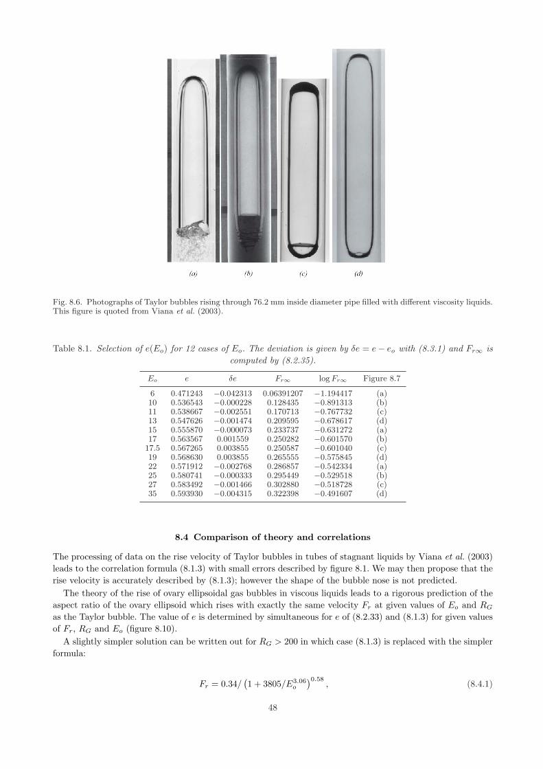
Fig. 8.6. Photographs of Taylor bubbles rising through 76.2 mm inside diameter pipe filled with different viscosity liquids.This figure is quoted from Viana et al. (2003).

Table 8.1. Selection of e(Eo) for 12 cases of Eo. The deviation is given by δe = e− eo with (8.3.1) and Fr∞ iscomputed by (8.2.35).

Eo e δe Fr∞ log Fr∞ Figure 8.7

6 0.471243 −0.042313 0.06391207 −1.194417 (a)10 0.536543 −0.000228 0.128435 −0.891313 (b)11 0.538667 −0.002551 0.170713 −0.767732 (c)13 0.547626 −0.001474 0.209595 −0.678617 (d)15 0.555870 −0.000073 0.233737 −0.631272 (a)17 0.563567 0.001559 0.250282 −0.601570 (b)

17.5 0.567265 0.003855 0.250587 −0.601040 (c)19 0.568630 0.003855 0.265555 −0.575845 (d)22 0.571912 −0.002768 0.286857 −0.542334 (a)25 0.580741 −0.000333 0.295449 −0.529518 (b)27 0.583492 −0.001466 0.302880 −0.518728 (c)35 0.593930 −0.004315 0.322398 −0.491607 (d)

8.4 Comparison of theory and correlations

The processing of data on the rise velocity of Taylor bubbles in tubes of stagnant liquids by Viana et al. (2003)leads to the correlation formula (8.1.3) with small errors described by figure 8.1. We may then propose that therise velocity is accurately described by (8.1.3); however the shape of the bubble nose is not predicted.

The theory of the rise of ovary ellipsoidal gas bubbles in viscous liquids leads to a rigorous prediction of theaspect ratio of the ovary ellipsoid which rises with exactly the same velocity Fr at given values of Eo and RG

as the Taylor bubble. The value of e is determined by simultaneous for e of (8.2.33) and (8.1.3) for given valuesof Fr, RG and Eo (figure 8.10).

A slightly simpler solution can be written out for RG > 200 in which case (8.1.3) is replaced with the simplerformula:

Fr = 0.34/(1 + 3805/E3.06

o

)0.58, (8.4.1)

48

-3.5

-3

-2.5

-2

-1.5

-1

-0.5

0

0 1 2 3 4 5 6

Eo=22

Eo=15

Eo=6

(a)

-3.5

-3

-2.5

-2

-1.5

-1

-0.5

0

0 1 2 3 4 5 6

Eo=25

Eo=17Eo=10

(b)

which is to be solved simultaneously with (8.2.33) in the limit RG →∞:

−F 2r e6

[e + (1− e2) tanh−1(e)

]2 +12

(1− e2

)=

8Eo

e2

1− e2, (8.4.2)

for e(Eo, RG) for given values of Eo (figure 8.10).

8.5 Conclusion

A formula is derived giving the rise velocity of an ellipsoidal gas bubble in a viscous liquid assuming that themotion of the liquid is irrotational. The rise velocity is expressed by a Froude number and it is determined bya Reynolds number, an Eotvos number and the aspect ratio of the ellipsoid. The formula for the ovary ellipsoidwas fit to the data of Viana et al. (2003) who correlated all the published data on the rise velocity of long gasbubbles in round tubes filled with viscous liquids. This data is accurately represented by our formula when theaspect ratio takes on certain values. The fitting generates a family of aspect ratios which depends strongly onthe Eotvos number and less strongly on the Reynolds number; this shows that the change in the shape of thenose of the rising bubble is strongly influenced by surface tension. Our analysis completely neglects sidewalldrainage induced by the rising bubble and cannot be a precise description of the dynamics. We have generatedwhat might be called the ovary ellipsoid model of a Taylor bubble. This model is very simple and astonishinglyaccurate.

49

-3.5

-3

-2.5

-2

-1.5

-1

-0.5

0

0 1 2 3 4 5 6

Eo=27

Eo=17.5Eo=11

(c)

-3.5

-3

-2.5

-2

-1.5

-1

-0.5

0

0 1 2 3 4 5 6

Eo=35

Eo=19Eo=13

(d)

Fig. 8.7. log Fr versus log RG for 12 values of Eo. The lines - - -, – – –, ——– are plots of (8.2.33) with e(Eo) selectedfor best fit as described in table 8.1.

50

0.2

0.4

0.6

0.8

1

1.2

1.4

1.6

1.8

2

-0.5 -0.45 -0.4 -0.35 -0.3 -0.25 -0.2 -0.15 -0.1 -0.05 0

Fig. 8.8. log Eo versus log e; 2 denotes the data given in table 8.1. The solid curve denotes the border Fr = 0 given by(8.2.37), above which one positive solution of Fr may exist and below which there arise two negative sollutions or complexsolutions which are meaningless. The dashed line is for Eo = 4. The dotted line denotes log e = 0.0865513 log Eo−0.356762for which eo = E0.0866

o /0.357.

0

0.25

0.5

0.75

1

0 0.25 0.5 0.75 1 1.25 1.5

r0/Rc=0.75

STAGNATION POINT

SYSTEM

AIR - WATERAIR - VARSOL

AIR - MARCOLAIR - PRIMOL

Fig. 8.9. Comparison of Brown’s 1965 measurements of the shape of a large Taylor bubble rising in a round tube withan ovary ellipsoid (denoted by the dashed line) with e = c/a = 0.6, b = a

√1− e2 = 0.8a, a = 1.10. Ovary ellipsoids with

smaller e are more spherical.

51

0.4

0.5

0.6

0.7

0.8

0 1 2 3 4 5 6

∞1000

100

RG=10

Fig. 8.10. e(Eo, RG) versus log Eo for various values of RG. The curves ——– are obtained by the simultaneous equations(8.1.3) and (8.2.33). The solution of (8.4.1) and (8.4.2) is shown as - - - - -; all the solutions (8.1.3) and (8.2.33) coincidewith - - - - - when RG > 104.

52

9

Rayleigh-Taylor instability of viscous fluids

Rayleigh-Taylor (hereafter RT) instabilities are very important and very pervasive. They are driven by accel-eration when a liquid acceleration away from a gas or vacuum. The signature of this instability is the waveswhich corrugate the free surface at the instant of acceleration. Ultimately these waves will finger into the liquidcausing it to break-up.

Rayleigh (1890) showed that a heavy fluid over a light fluid is unstable, as common experience dictates. Hetreated the stability of heavy fluid over light fluid without viscosity, and he found that a disturbance of the flatfree surface grows exponentially like exp (nt) where

n =

kg (ρ2 − ρ1)ρ1 + ρ2

1/2

, (9.0.1)

where ρ2 is the density of the heavy fluid, ρ1 is the density of the light fluid, g is the acceleration due to gravityand k = 2π/` is the wavenumber and ` is the wavelength. The instability described by (9.0.1) is catastrophicsince the growth rate n tends to infinity, at any fixed time, no matter how small, as the wavelength tends tozero. The solutions are unstable to short waves even at the earliest times. Such disastrous instabilities are called‘Hadamard unstable’ and the initial value problems associated with these instabilities are said to be ‘ill posed’(Joseph & Saut 1990). Ill-posed problems are disasters for numerical simulations: because they are unstable toever shorter waves, the finer the mesh, the worse the result.

Nature will not allow such a singular instability; for example, neglected effects like viscosity and surfacetension will enter the physics strongly at the shortest wavelength. These effects have been taken into accountin the study of RT instability by Harrison (1908) and in treatise of Chandrasekhar (1961). Surface tensioneliminates the instability of the short waves; there is a finite wavelength depending strongly on viscosity aswell as surface tension for which the growth rate n is maximum. This is the wavelength that should occur ina real physical problem and would determine the wavelength on the corrugated fronts of breaking drops in ahigh-speed air flow.

Taylor (1950) extended Rayleigh’s inviscid analysis to the case where a constant acceleration of the superposedfluids other than gravity is taken into account. Assuming a constant value for the acceleration, Taylor (1950)showed that when two superposed fluids of different densities are accelerated in a direction perpendicular totheir interface, this surface is unstable if the acceleration is directed from the lighter to the heavier fluid. TheTaylor instability depends strongly on the value of the acceleration a; for example, if g in (9.0.1) is replaced bya = 104g, the growth rate n is increased by a factor of 100.

9.1 Acceleration

The acceleration of the drop is a major factor in the Rayleigh-Taylor (RT) instability. It is instructive to seehow the acceleration enters into the equations of motion. Suppose the laboratory frame is identified with

(X, t

)and the drop velocity is v(X, t). Then we refer the equations of motion

ρ

(∂v

∂t+ v · ∂v

∂X

)= divT + ρg,

∂

∂X· v = 0 (9.1.1)

53

Fig. 9.1. RT instability: (a) the liquid in the containers at rest is stable under gravity (Rayleigh 1890) but if the containeris turned upside down as in (c) the liquid falls out. The liquid at rest in container can be destabilized by downwardacceleration of the liquid a > g away from gas as in (b) and in the upside down case the liquid can be prevented from

falling out by accelerating downward with V > g as in (d). If we open up the container and accelerates the liquid

downward with V > g, the top surface which accelerates away from the gas is unstable but the bottom surface whichaccelerates into the gas is stabilized as in (e), with the opposite effect when the acceleration is reversed as in (f).

to an accelerating frame in which the mass center of the drop is stationary, identified with (x, t) and v(X, t) =U(x, t) + V (t), dX = dx + V (t)dt, dt = dt. Then we find that

ρ

(∂U

∂t+ U · ∂U

∂x

)+ ρV = divT + ρg ,

∂

∂x· U = 0 (9.1.2)

where T is the stress tensor.The term

ρ(g − V

)(9.1.3)

enters into Rayleigh-Taylor instability and V dominates in the drop breakup problem because the initial velocityis very small and the initial acceleration is very large.

The Rayleigh-Taylor instability occurs when V is directed from the light to the heavy fluid as when theinitially stationary drop is accelerated to the free-stream velocity in the high-speed air stream behind the shockin the shock tube or when a moving drop in a stagnant fluid is decelerated by the air to zero velocity. Theanalysis works well in air and liquid where the density and viscosity of air can be neglected with only smallerror; there is Rayleigh-Taylor instability in a vacuum because it is the drop acceleration term and not thematerial properties of air which induces the instability.

In the present application the acceleration of the drop is roughly proportional to the dynamic pressure whichvanishes in a vacuum. Drop breakup in a vacuum could occur by acceleration due to gravity, say in a rarifiedJovian atmosphere.

9.2 Simple thought experiments

These experiments are embodied in the cartoons and caption of figure 9.1. These experiments show the differencebetween the theory of Rayleigh (1890) who considered gravity g and Taylor (1950) who considered the effectof the acceleration V . The accelerations destabilize the liquid-gas surfaces which accelerate away from the gasand stabilize the liquid-gas surface which accelerate toward the gas (figure 9.1 (e)).

9.3 Analysis

The linear theory of stability superposes small disturbances on a basic flow solution of the equations of motion.Nonlinear terms in small perturbation quantities are neglected. The properties of the basic flow are important.The basic flow for RT instability deserves consideration. Here we look for conditions under which corrugationsappear on flat free surface on a liquid moving into or away from a gas or vacuum. What is important here is theacceleration and the fact that shear stresses do not develop in the basic flow. This is, of course, is even clearerif you take the gas away and leave a vacuum. In this chapter and in chapter 21 on RT instability of viscoelasticdrops, we are obliged to consider RT instability on the front face of a flattened drops in which Kelvin-Helmholtz(KH) instability driven by shearing motion may play a minor role.

Lewis (1950) has shown experimentally that a layer of water driven by compressed air is unstable and thatsmall disturbances, introduced at the air-water interface, grow so that it appears as though fingers of air move

54

through the water layer. Lewis (1950) finds agreement with his experiments when the viscosity of the liquid issmall. The peaks of water in his experiments are sharp, but the match between Taylor’s theory and the Lewisexperiment is not perfect because the regularizing effects of surface tension were neglected.

The breakup of water drops in a high speed air behind a shock wave in a shock tube was studied in excellentexperiments by Engel (1958). Since the acceleration is perpendicular to the air-liquid interface and directed fromgas to liquid, the accelerating liquid drop is unstable and is prey to the characteristic short wave corrugationassociated with this instability.

Joseph, Belanger and Beavers (1999) (hereafter JBB) studied the breakup of liquid drops of high and lowviscosity and viscoelastic drop in high air behind shock waves moving at Mach numbers Ms = 2 and Ms = 3.They measured acceleration and wave lengths on the corrugation drops.

The corrugations at the front of an unstable drop are driven toward the drop equator by shear flow of gascoming from the high pressure stagnation point. This shear flow may also be subject to an instability of theKelvin-Helmholtz type. Since the tangential velocity is zero at the stagnation point and small near the stagnationpoint, the Kelvin-Helmholtz instability may not interact too strongly with the Rayleigh-Taylor instability.

Some details of the corrugations on the front of breaking drops can be predicted by mathematical analysisof the foregoing instabilities, but the effects of viscosity and surface tension must be taken into account.

9.3.1 Linear theory of Chandrasekhar

A thorough explanation and analysis of the Rayleigh-Taylor instability can be found in Chapter X of thetreatise by Chandrasekhar. Some effects of viscosity in special problems in Rayleigh-Taylor instability havebeen considered by Plesset and Whipple (1973). In Chandrasekhar’s analysis the two fluids are separated byan interface z = h(x, y, t) which perturbs the plane z = 0. The Navier-Stokes equations for the perturbationsvelocity u, perturbation pressure p are solved above and below the plane z = 0. Gravity points down againstthe direction of z increasing. It is assumed that the heavy fluid is above the light fluid, or that the light fluid isaccelerated into the heavy fluid above (the drop is the heavy fluid and the gas flowing into and around it is thelight fluid). At the flat interface at z = 0, the linearized kinematic equation is

w =∂h

∂t(9.3.1)

where

[|w|] = w2 − w1 (9.3.2)

is the jump in the normal (z component) of velocity (w2 is in z > 0, w1 in z < 0). For the viscous case the jumpin the tangential velocity is also zero

[|w|] = [|u|] = [|v|] = 0 (9.3.3)

where u is in the x direction and v in the y direction. Since (9.3.3) holds for all x and y for z = 0, we maydeduce that

[∣∣∣∣∂u

∂x+

∂v

∂y

∣∣∣∣]

= −[∣∣∣∣

∂w

∂z

∣∣∣∣]

= 0 (9.3.4)

The continuity of the shear stress is expressed by[∣∣∣∣µ

(∂u

∂z+

∂w

∂x

)∣∣∣∣]

= 0,

[∣∣∣∣µ(

∂v

∂z+

∂w

∂y

)∣∣∣∣]

= 0 (9.3.5)

where µ is the viscosity.The balance of normal stress is given by

− [|p|] + 2[∣∣∣∣µ

∂w

∂z

∣∣∣∣]

= −γ

(∂2

∂x2+

∂2

∂y2

)h (9.3.6)

where γ is the surface tension. We may remove the hydrostatic pressure from the z equation of motion byintroducing the dynamic pressure

π = p + ρgh

55

hence,

[|π|] = gh [|ρ|] + 2[∣∣∣∣µ

∂w

∂z

∣∣∣∣]

+ γ

(∂2

∂x2+

∂2

∂y2

)h (9.3.7)

After introducing normal modes proportional to

f(z)ent+ıkxx+ıkyy, k2 = k2x + k2

y (9.3.8)

where f(z) is an amplitude function for π, u, v and h which may be eliminated to find equation (40) on page433 of Chandrasekhar:

[∣∣∣∣[

ρ− µ

n

(d2

dz2− k2

)]dw

dz− 1

n

(d2

dz2+ k2

)w

dµ

dz

∣∣∣∣]

= −k2

n2

g [|ρ|]− k2γ

w − 2k2

n

[∣∣∣∣µdw

dz

∣∣∣∣]

. (9.3.9)

For the present problem for which the unperturbed states above and below z = 0 are uniform dµ/dz = 0 and,using (9.3.4)

[∣∣∣∣µdw

dz

∣∣∣∣]

= [|µ|] dw

dz. (9.3.10)

The entire problem is resolved by

w1 = A1ekz + B1eq1z (z < 0)

w2 = A2e−kz + B2e−q2z (z > 0) (9.3.11)

where

q1 =√

k2 + n/ν1 and q2 =√

k2 + n/ν2

ν1 = µ1/ρ1, ν2 = µ2/ρ2 (9.3.12)

provided that Chandrasekhar’s equation (113) below is satisfied

−

gk

n2

[(α1 − α2) +

k2γ

g (ρ1 + ρ2)

]+ 1

(α2q1 + α1q2 − k)− 4kα1α2 +

4k2

n(α1ν1 − α2ν2)

×(α2q1 − α1q2) + k (α1 − α2)+4k3

n2(α1ν1 − α2ν2)

2 (q1 − k )( q2 − k) = 0 (9.3.13)

where

α1 =ρ1

ρ1 + ρ2, α2 =

ρ2

ρ1 + ρ2, α1 + α2 = 1

When the light fluid is gas; with only a very small error we may treat this as a vacuum. Hence we put

ρ1 = α1 = 0, α2 = 1

q1 → k, α2q1 + α1q2 − k → q1 − k

(α2q1 − α1q2) + k (α1 − α2) → q1 − k (9.3.14)

and, after factoring q1 − k in (9.3.13) we get

1− gk

n2= − k3γ

n2ρ2− 4k2

n

µ2

ρ2+

4k3

n2

µ22

ρ22

(q2 − k) . (9.3.15)

9.3.2 Viscous potential flow

The Rayleigh-Taylor instability may also be analyzed as a viscous potential flow (Joseph, 1994). In this approachthe perturbation velocity is given by a potential

u = ∇φ (9.3.16)

and the Navier-Stokes equations are reduced to an identity provided that the pressure is given by Bernoulli’sequation

p + ρ∂φ

∂t+ ρgz = −ρ

2|∇φ|2 . (9.3.17)

56

In this linearization used to study instability the term on the right side of (9.3.17) is put to zero. The interfacecondition requires continuity of tangential velocities, (9.3.3) and (9.3.4), and the continuity of shear stress (9.3.5)cannot be enforced in viscous potential flow. The pressure in the normal stress condition (9.3.6) is eliminatedusing (9.3.17); this gives rise to

[∣∣∣∣ρ∂φ

∂t

∣∣∣∣]

+ gh[|ρ|] + 2[∣∣∣∣µ

∂w

∂z

∣∣∣∣]

+ γ

∂2

∂x2+

∂2

∂y2

h = 0. (9.3.18)

After introducing normal modes, writing (9.3.1) as nh = w, we get

n[|ρφ|] +w

n[|ρ|]g + 2

[∣∣∣∣µ∂w

∂z

∣∣∣∣]− γk2

nw = 0 (9.3.19)

For viscous potential flow, ∇2φ = 0 everywhere and (9.3.11) holds with B1 = B2 = 0 and

dw

dz=

d2φ

dz2= k2φ. (9.3.20)

After writing [|ρφ|] = (1/k2)[|ρdw/dz|] in (9.3.19) we may verify that (9.3.9) and (9.3.19) are identical when(9.3.9) is evaluated for viscous potential flow. Further evaluation of (9.3.19) with normal modes give rise to thedispersion relation

1 =k

n2

ρ2 − ρ1

ρ2 + ρ1g − k3γ

n2(ρ2 + ρ1)− 2k2

n

µ2 + µ1

ρ2 + ρ1. (9.3.21)

Equation (9.3.21) may be solved for the growth rate

n = −k2 µ2 + µ1

ρ2 + ρ1±

[k

ρ2 − ρ1

ρ2 + ρ1g − k3γ

ρ2 + ρ1+ k4

(µ2 + µ1

ρ2 + ρ1

)2]1/2

(9.3.22)

If the quantity under the root is negative, then the real part is negative and the interface is stable. For instabilityit is sufficient that

√k

ρ2 − ρ1

ρ2 + ρ1g + k4

(µ2 + µ1

ρ2 + ρ1

)2

− k3γ

ρ2 + ρ1> k2 µ2 + µ1

ρ2 + ρ1. (9.3.23)

The border of instability n = 0 for k = kc is given by

kc =

√(ρ2 − ρ1)g

γ(9.3.24)

independent of viscosity.Evaluation of the growth rate formula with the gas neglected gives

n = −k2µ2

ρ2±

√kg − k3γ

ρ2+

k4µ22

ρ22

(9.3.25)

It is of interest to compare the growth rate formula (9.3.25) for viscous potential flow with the growth rateformula (9.3.15) for Chandrasekhar’s exact solution. These two formulas give exactly the same growth rate when

q2 − k = k

√1 +

nρ2

µ2k2− k ∼= nρ2

2µ2k(9.3.26)

andnρ2

2µ2k¿ 1 (9.3.27)

9.4 Comparison of theory and experiments

To evaluate the formulas for Rayleigh-Taylor instability for the experiments of JBB we must

replace g with a = V . (9.4.1)

57

Fig. 9.2. Growth rate curve.

Equation (9.3.24) then implies that

kc =2π

λc=

√ρ2a

γ(9.4.2)

and waves with length

λ < λc = 2π

√γ

ρ2a(9.4.3)

are stable. Taking liberties with (9.4.3), we identify λ = D where D is the diameter of drops with acceleration a

that cannot be fragmented by Rayleigh-Taylor instability. Applying this to our experiments (table 9.1) we getD between

23 and 65µm for MS = 3 (9.4.4)

46 and 135µm for MS = 2. (9.4.5)

A typical growth rate curve for the parameters in (9.4.4) and in (9.4.5) is shown by Fig.9.2.

9.5 Comparison of the stability theory with the experiments on drop breakup

JBB studied the breakup of liquid drops of high and low viscosity behind a shock wave in a shock tube movingwith shock Mach number Ms = 2 and Ms = 3. The data for the experiments is listed in table 2 of JBBtogether with values of the dimensionless parameters. The Ohnesorge number Oh, the Weber number We andthe Reynolds number Re

Oh =µd

(ρdDγ)1/2, We =

ρV 2D

γ, Re =

V Dρ

µ(9.5.1)

are defined in terms of the initial drop diameter D, drop viscosity µd, surface tension γ, drop density ρd, andthe free stream values of the velocity V , viscosity µ, and density ρ.

The breakup of drops in high speed airstream behind a shock wave in a shock tube was photographed witha rotating drum camera giving one photograph every 5 µs. From these photographs, JBB created movies of thefragmentation history of viscous drops of widely varying viscosity, and viscoelastic drops, at very high Weber andReynolds numbers. Drops of the order of one millimeter are reduced to droplet clouds and possibly to vapor intimes less than 500 µs. The movies may be viewed at http://www.aem.umn.edu/research/Aerodynamic Breakup.They reveal sequences of breakup events which were previously unavailable for study. Bag and bag-and-stamenbreakup can be seen at very high Weber numbers, in the regime of breakup previously called ‘catastrophic.’The movies generate precise displacement-time graphs from which accurate values of acceleration (of orders 104

to 105 times the acceleration of gravity) are computed. These large accelerations from gas to liquid put theflattened drops at high risk to Rayleigh-Taylor instabilities. The most unstable Rayleigh-Taylor wave fits nearlyperfectly with waves measured on enhanced images of drops from the movies, but the effects of viscosity cannotbe neglected.

The breakup of drops in a high speed air stream exhibits universal features. First the shock wave passes over

58

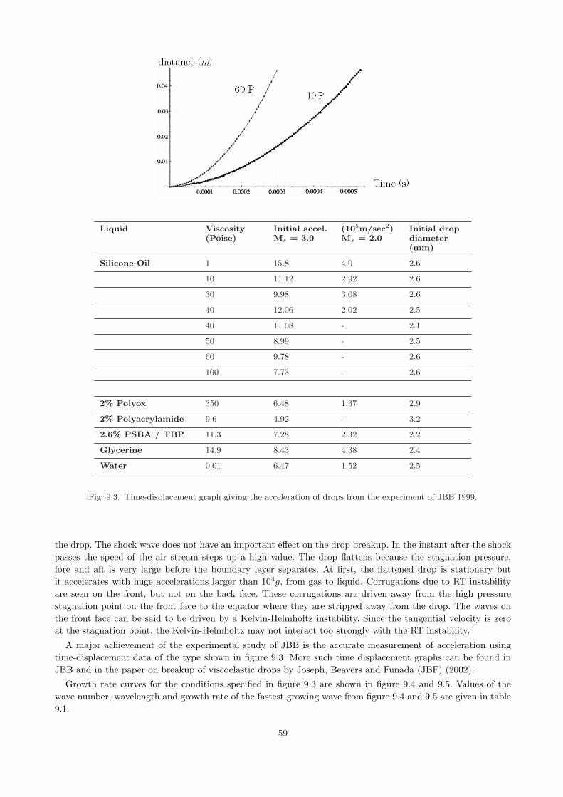
Liquid Viscosity(Poise)

Initial accel.Ms = 3.0

(105m/sec2)Ms = 2.0

Initial dropdiameter(mm)

Silicone Oil 1 15.8 4.0 2.6

10 11.12 2.92 2.6

30 9.98 3.08 2.6

40 12.06 2.02 2.5

40 11.08 - 2.1

50 8.99 - 2.5

60 9.78 - 2.6

100 7.73 - 2.6

2% Polyox 350 6.48 1.37 2.9

2% Polyacrylamide 9.6 4.92 - 3.2

2.6% PSBA / TBP 11.3 7.28 2.32 2.2

Glycerine 14.9 8.43 4.38 2.4

Water 0.01 6.47 1.52 2.5

Fig. 9.3. Time-displacement graph giving the acceleration of drops from the experiment of JBB 1999.

the drop. The shock wave does not have an important effect on the drop breakup. In the instant after the shockpasses the speed of the air stream steps up a high value. The drop flattens because the stagnation pressure,fore and aft is very large before the boundary layer separates. At first, the flattened drop is stationary butit accelerates with huge accelerations larger than 104g, from gas to liquid. Corrugations due to RT instabilityare seen on the front, but not on the back face. These corrugations are driven away from the high pressurestagnation point on the front face to the equator where they are stripped away from the drop. The waves onthe front face can be said to be driven by a Kelvin-Helmholtz instability. Since the tangential velocity is zeroat the stagnation point, the Kelvin-Helmholtz may not interact too strongly with the RT instability.

A major achievement of the experimental study of JBB is the accurate measurement of acceleration usingtime-displacement data of the type shown in figure 9.3. More such time displacement graphs can be found inJBB and in the paper on breakup of viscoelastic drops by Joseph, Beavers and Funada (JBF) (2002).

Growth rate curves for the conditions specified in figure 9.3 are shown in figure 9.4 and 9.5. Values of thewave number, wavelength and growth rate of the fastest growing wave from figure 9.4 and 9.5 are given in table9.1.

59

Fig. 9.4. n (sec−1) vs. k (cm−1) for viscous potential flow; shock Mach number = 2.

The parameters of the maximum growth rate computed by VPF are in excellent agreement with the exactsolution.

9.6 Comparison of the measured wavelength of corrugations on the drop surface with theprediction of the stability theory

We have shown that the theoretical prediction about stability depends very strongly on viscosity and that thisdependence is very well predicted by a purely irrotational theory. It remains to show that these predictionsagree with experiments. JBB compared photos from their movies with the stability theory predicted in section9.3. No special choice was made in selecting the frames for the comparisons other than choosing ones from theearly part of the motion that were well focused. The wave-like structute can be identified much more easilyon the computer screen than in the images reproduced in figures 1-13 of JBB. In figure 9.6 the predicted andobserved wavelengths on a water drop at Ms = 2 and 3 are compared. The tick marks on the photos identifywave troughs so that the predicted distance between the tick marks is the length of an unstable wave. The samekind of comparison is given in figure 9.7 for silicone oil in figure 9.8 for glycerine.

In figure 9.9 (which is figure 14 in JBF) we show the analysis of RT waves can be enhanced by imageprocessing.

Stages of breakup of water drops at Ms = 2 and Ms = 3 are shown in figures 9.10 and 9.11. RT waves appearon the front face immediately and the drop is reduced to mist in 200 µs. Very excellent photographs of thefragmentation of water drops to mist can be found in the paper of O.Engel (1958).

The agreements between theory and experiment may extend to high viscosity drop. The lengths of the mostunstable waves are greater than the diameter of the drops. Waves shorter than those which grow fastest growmore slowly. The retardation of the instability of unstable waves which is predicted by theory is realized byexperiments; the larger the viscosity the larger is the length of time it takes for the drop to break. Eventuallythey do break and the breakup looks like a bag breakup as in figure 9.10.

60

Fig. 9.5. n (sec−1) vs. k (cm−1) for viscous potential flow; shock Mach number = 3.

Fig. 9.6. Rayleigh-Taylor Waves in Water. The tick marks on the photographs locate wave troughs.

9.7 Fragmentation of Newtonian and viscoelastic drops

The breakup of drops in a high speed air flow is a fundamental problem of two-phase fluid and it has given riseto a large literature. Most of the early literature focuses on drops of Newtonian liquids in subsonic air streams,and is excellently reviewed by Pilch & Erdman (1987), and Hsiang and Faeth (1992). Shock tube studies of thebreakup of Newtonian drops, usually water, under high subsonic and supersonic conditions were carried outby Hanson and Domich (1956), Engel (1958), Hanson, Domich, & Adams (1963), Ranger and Nicholls (1969),Reinecke & McKay (1969), Reinecke & Waldman (1970, 1975), Waldman, Reinecke & Glenn (1972), Simpkins& Bales (1972), Wierzba and Takayama (1988), Yoshida & Takayama (1990), Hirahara and Kawahashi (1992),

61

Table 9.1. Values of the wave number, wave length, and growth rate of the most dangerous wave for theexperimental conditions given in tables 1 and 2 of JBB.

Liquid Viscosity Exact Viscous Potential

(kg/m/s) n (sec−1) k (cm−1) λ (mm) n (sec−1) k (cm−1) λ (mm)

Ms = 3SO 10000 10 17790 9.5 6.61 19342 9.7 6.48SO 6000 6 24673 14.45 4.35 26827 14.7 4.27SO 5000 5 24787 15.86 3.96 26951 16.15 3.89SO 4000 4 32550 20.3 3.10 35312 20.7 3.04SO 3000 3 31507 23.08 2.72 34257 23.5 2.67SO 1000 1 48769 49.68 1.26 53088 50.65 1.24SO 100 0.1 132198 253.2 0.25 143699 259 0.24Glycerine 1.49 38760 41.3 1.52 42141 42.1 1.492% PO 35 10492 3.95 15.91 11406 3.95 15.912.6% PSBA 1.13 34460 37.8 1.66 37467 38.5 1.632% PAA 0.96 28927 39.4 1.59 31451 40.15 1.56Water 0.001 149632 531.95 0.12 151758 540.8 0.12Ms = 2SO 4000 4 9868 11.2 5.61 10729 11.4 5.51SO 3000 3 14388 15.6 4.03 15644 15.9 3.95SO 1000 1 20018 31.8 1.98 21765 32.4 1.94SO 100 0.1 52726 158 0.40 57304 161.9 0.39Glycerine 1.49 25046 33.2 1.89 27231 33.8 1.862% PO 35 3723 2.35 26.74 4048 2.4 26.182.6% PSBA 1.13 16070 25.75 2.44 17472 26.25 2.39Water 0.001 50971 260.9 0.24 51507 264.2 0.24

Fig. 9.7. Rayleigh-Taylor Waves in Silicone Oil (0.1 kg/msec). The tick marks on the photographs locate wave troughs.

and others. The excellent study of Engel (1958) showed that water drops of millimeter diameter would bereduced to mist by the flow behind an incident shock moving at Mach numbers in the range 1.3 to 1.7. Many ofthe other aforementioned studies allude to the presence of large amounts of mist. Joseph, Huang and Candler(1996) argued that mist could arise from condensed vapor under flash vaporization due to (1) low pressures atthe leeside produced by rarefaction and drop acceleration, (2) high tensions produced by extensional motions inthe liquid stripped from the drop, (3) the frictional heating by rapid rates of deformation, and (4) the heatingof sheets and filaments torn from the drop by hot air. Though mist and vapor formation is not the focus of thisstudy, it is relevant that the Rayleigh-Taylor instability pumps fingers of hot gas, behind the shock, into thedrop increasing both the frictional heating and the area of liquid surface exposed to hot gas. The recent andfairly extensive literature on atomization is well represented in the papers by Hsiang and Faeth (1992), Hwang,Liu and Rietz (1996), and Faeth (1996). These results, and earlier drop breakup studies such as Krzeczkowski(1980), Wierzba (1990), Kitscha and Kocamustafaogullari (1989), and Stone (1994), are restricted to relativelylow Weber and Reynolds numbers. The highest Weber and Reynolds data for drop breakup was reported by

62

Fig. 9.8. Rayleigh-Taylor waves in glycerine. The tick marks on the photographs locate wave troughs.

Hsiang and Faeth (1992) who worked under conditions for which the Weber numbers ranged from 0.5 to 1000with Reynolds numbers from 300 to 1600.

High Weber number drop breakup data were obtained by Engel (1958), Ranger and Nichols (1969), andReinecke and Waldman (1970) for air and water only, so viscous effects could not be studied. In contrast,the data presented here cover a wide range of viscosities (from 0.001 to 35 kg/m sec) and a wide range of highWeber numbers (from 11,700 to 169,000), Ohnesorge numbers (from 0.002 to 82.3) and Reynolds numbers (from40,000 to 127,600), based on the free stream conditions. Another feature which distinguishes the experimentsof JBB from previous ones is that they recorded all of the data as real time movies which may be seen under‘video animations’ at the Web address http://www.aem.umn.edu/research/Aerodynamic Breakup/. The moviescapture events which were previously unknown, such as bag breakup and bag-and-stamen breakup of highviscosity drops at very high Weber numbers, whereas short wave Rayleigh-Taylor corrugations appear on waterdrops under similar free stream conditions.

Only a few studies of the breakup of viscoelastic drops have been published; Lane (1951), Wilcox, June, Braunand Kelly (1961), Matta and Tytus (1982), and Matta, Tytus and Harris (1983). Matta and co-workers didstudies at Mach numbers near one and less. They showed that threads and ligaments of liquid arise immediatelyafter breakup, rather than the droplets which are seen in Newtonian liquids. Breakup of viscoelastic drops areshown in figure 9.9 and in many photographs shown by JBF 2002.

9.8 Modelling Rayleigh-Taylor instability of a sedimenting suspension of several thousandcircular particles in a direct numerical simulation

Pan, Joseph and Glowinski (2000) studied the sedimentation of several thousand circular particles in twodimensions using the method of distributed Lagrange multipliers for solidliquid flow. The simulation gives riseto fingering which resembles Rayleigh-Taylor instabilities. The waves have a well-defined wavelength and growthrate which can be modelled as a conventional Rayleigh-Taylor instability of heavy fluid above light. The heavyfluid is modelled as a composite solid-liquid fluid with an effective composite density and viscosity. Surfacetension cannot enter this problem and the characteristic shortwave instability is regularized by the viscosity ofthe solid-liquid dispersion. The dynamics of the Rayleigh-Taylor instability are studied using viscous potentialflow, generalizing work of JBB to a rectangular domain bounded by solid walls; an exact solution is obtained.The model shows the same trends as the simulation but it allows the effective fluid to slip at the side-walls. Themodel with slip at the side walls is very easily constructed, but an analytic solution with no-slip at the side wall

63

Fig. 9.9. (JBF, figure 14) (a) Rayleigh-Taylor waves in 2% aqueous polyox in the flow behind a Mach 2.9 shockwave. Time(in µs) after passage of shock: (i) 30, (ii) 35, (iii) 40, (iv) 45. (b) Movie frames corresponding to the contrast-enhancedimages of (a).

is not known and apparently cannot be found by the method of separation of variables. It is probable that thenumerical simulation would be better modeled by continuum model with no-slip at side walls.

Sample pictures of the simulation are shown in figures 9.13 and 9.14. The formation of RT instability followsthe acceleration guidelines in the cartoon of fgure 9.1(e); the top surface is flat ad the bottom one is corrugated.

64

Fig. 9.10. Stages in the breakup of a water drop (diameter = 2.6 mm) in the flow behind a Mach 2 shock wave. Airvelocity = 432 m/s; dynamic pressure = 158.0 kPa; Weber No. = 11,700. Time (µs): (a) 0, (b) 45, (c) 70, (d) 135, (e)170, (f) 290.

Fig. 9.11. Stages in the breakup of a water drop (diameter = 2.5 mm) in the flow behind a Mach 3 shock wave. Airvelocity = 764 m/s; dynamic pressure = 606.4 kPa; Weber No. = 43,330. Time (µs): (a) 0, (b) 15, (c) 30, (d) 40, (e) 95,(f) 135.

65

Fig. 9.12. Stages in the breakup of a drop of glycerine (diameter = 2.4 mm) in the flow behind a Mach 3 shock wave.Air velocity = 758 m/s; dynamic pressure = 554.0 kPa; Weber No. = 42,220. Time (µs): (a) 0, (b) 35, (c) 50, (d) 70, (e)90, (f) 125, (g) 150, (h) 185.

66

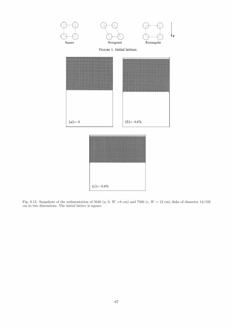
Fig. 9.13. Snapshots of the sedimentation of 5040 (a; b, W =8 cm) and 7560 (c, W = 12 cm) disks of diameter 14/192cm in two dimensions. The initial lattice is square.

67

Fig. 9.14. Snapshots of the sedimentation of 4800 (a; b) and 6400 (c; d) disks in two dimensions (W = 8 cm). Thediameter of disks in (a), (b) and (c) is 10/192 cm and the diameter of disks in (d) is 16/192 cm. The initial lattice isrectangular.

68

10

The force on a cylinder near a wall in viscouspotential flows

We study the force on a two-dimensional cylinder near a wall in two potential flows: the flow due to thecirculation 2πκ about the cylinder and the uniform streaming flow with velocity V past the cylinder. Thepressure is computed using the Bernoulli equation and the viscous normal stress is calculated using viscouspotential flow; the shear stress is ignored. The forces on the cylinder are computed by integration of the normalstress over the surface of the cylinder. In both of the two cases, the force perpendicular to the wall (lift) is onlydue to the pressure and the force parallel to the wall (drag) is only due to the viscous normal stress. Our resultsshow that the drag on a cylinder near a wall is larger than on a cylinder in an unbounded domain. In the flowinduced by circulation or in the streaming flow, the lift force is always pushing the cylinder towards the wall.However, when the two flows are combined, the lift force can be pushing the cylinder away from the wall ortowards the wall.

10.1 The flow due to the circulation about the cylinder

Figure 10.1 shows a cylinder with radius a near the wall x = 0. Let b be the distance of the axis of the cylinderfrom the wall and c = OP where OP is the tangent of the cylinder. The complex potential for the flow due tothe anti-clockwise circulation 2πκ about the cylinder is (Milne-Thomson, 1968 §6.53)

ω = −2κcot−1 ız

c. (10.1.1)

To facilitate the calculation, we introduce a parameter η, so that

a = c cschη and b = c cothη. (10.1.2)

x

y

a

Q

b

O

Pc

Fig. 10.1. A cylinder with radius a near the wall x = 0.

69

We can also express c and η in terms of a and b:

c =√

b2 − a2 and η = cosh−1(b/a). (10.1.3)

The complex velocity is

u− ıv =dω

dz=

2ıcκ

c2 − z2. (10.1.4)

We separate the real and imaginary parts of the velocity to obtain

u =−4cκxy

(c2 − x2 + y2)2 + 4x2y2and v =

−2cκ(c2 − x2 + y2)(c2 − x2 + y2)2 + 4x2y2

. (10.1.5)

The pressure can be computed using the Bernoulli equation

p + ρ|u|2/2 = Const ⇒ −p = ρ|u|2/2− Const. (10.1.6)

The rate of strain tensor can be evaluated

2D =[

2∂u/∂x ∂u/∂y + ∂v/∂x

∂u/∂y + ∂v/∂x 2∂v/∂y

]. (10.1.7)

The surface of the cylinder can be expressed as

x = c cothη + c cschη cosθ, y = c cschη sinθ, (10.1.8)

where 0 6 θ 6 2π. The normal on the surface of the cylinder is

n = cosθex + sinθey. (10.1.9)

The viscous normal stress at the surface is

τnn = n · 2µD · n = 2µ

[∂u

∂xcos2θ +

(∂u

∂y+

∂v

∂x

)sinθcosθ +

∂v

∂ysin2θ

]

=−2µκ sinθ sinh3η

c2 (cosθ + coshη)2, (10.1.10)

and the pressure at the surface is

− p =ρ

2κ2sinh4

c2 (cosθ + coshη)2− Const. (10.1.11)

The forces on the cylinder by the normal stress are

Fx =∫ 2π

0

(−p + τnn) cosθ c cschη dθ, Fy =∫ 2π

0

(−p + τnn) sinθ c cschη dθ. (10.1.12)

We calculate the contributions to the forces by the pressure and viscous stress separately. The superscript “p”and “v” stand for pressure and viscous stress, respectively. The forces by the pressure are

F px =

∫ 2π

0

ρκ2sinh3η

2c

cosθ dθ

(cosθ + coshη)2= −πρκ2

c, (10.1.13)

F py =

∫ 2π

0

ρκ2sinh3η

2c

sinθ dθ

(cosθ + coshη)2= 0, (10.1.14)

which agree with the values computed using the theorem of Blasius (Milne-Thomson, 1968 §6.53). The forcesby the viscous stress are

F vx =

∫ 2π

0

−2µκ sinh2η

c

sinθcosθ dθ

(cosθ + coshη)2= 0, (10.1.15)

F vy =

∫ 2π

0

−2µκ sinh2η

c

sinθsinθ dθ

(cosθ + coshη)2= −2πµκ

c

(1− e−2η

). (10.1.16)

70

1 3 5 7 90

0.5

1

1.5

2

2.5

3

3.5

4

b/a

| Cx| o

r | C

y|

| Cx|

| Cy|

Fig. 10.2. The absolute values of the coefficients for the force |Cx| and |Cy| as functions of the ratio b/a. The Reynoldsnumber is taken as 1 when computing Cy.

Using equation (10.1.3), the forces can be expressed in terms of a and b:

Fx = F px + F v

x = − πρκ2

√b2 − a2

, (10.1.17)

Fy = F py + F v

y = − 2πµκ√b2 − a2

(1− e−2cosh−1(b/a)

). (10.1.18)

We define a characteristic velocity U = 2πκ/a and make the forces dimensionless.

Cx =Fx

12ρU2a

= − 12π

√(b/a)2 − 1

, (10.1.19)

Cy =Fy

12ρU2a

= − 4Re

1√(b/a)2 − 1

[1− e−2cosh−1(b/a)

], (10.1.20)

where Re = ρU2a/µ is the Reynolds number. Here Cx is a function of the ratio b/a only; Cy is a function ofb/a and Re. We plot |Cx| and |Cy| as functions of b/a in Figure 10.2. The Reynolds number is taken as 1 whencomputing Cy. When b/a approaches 1, meaning that the gap between the wall and the cylinder is very small,both of the two forces approach infinity. When b/a approaches infinity, both of the two forces approach zero,because the interaction between the cylinder and the wall is negligible.

10.2 The streaming flow past the cylinder near a wall

The domain is bounded by the plane x = 0 and the cylinder (x− b)2 + y2 = a2(Figure 10.1). The uniform flowwith the velocity V at infinity is streaming in the negtive direction of the y axis. The complex potential for theflow is (Milne-Thomson, 1968 p. 185)

ω = ıV z − 2ıV a2z

[1

z2 − b2+

∞∑n=1

a2n

∏n−1r=0 (b + xr)2(z2 − x2

n)

], (10.2.1)

where x0 = b, xn = b− a2/(b + xn−1). The potential is represented by an infinite series which converges rapidlyfor moderate or large values of the ratio b/a. To carry out the calculation, we consider the terms up to n = 3in (10.2.1):

ω = ıV z − 2ıV a2z

[1

z2 − b2+

a2

β1(z2 − x21)

+a4

β2(z2 − x22)

+a6

β3(z2 − x23)

](10.2.2)

71

where

x1 = b− a2

2b, x2 = b− a2

2b− a2/(2b), x3 = b− a2

2b− a2

2b−a2/(2b)

; (10.2.3)

β1 = (2b)2, β2 = (2b)2(

2b− a2

2b

)2

, β3 = (2b)2(

2b− a2

2b

)2 [2b− a2

2b− a2/(2b)

]2

. (10.2.4)

The complex velocity is dω/dz and we separate the real and imaginary parts of it to obtain the velosities in x

and y directions.

u =− 4a2V xy

(x2 − y2 − b2)2 + 4x2y2− 4a4V xy

β1[(x2 − y2 − x21)2 + 4x2y2]

− 4a6V xy

β2[(x2 − y2 − x22)2 + 4x2y2]

− 4a8V xy

β3[(x2 − y2 − x23)2 + 4x2y2]

+8a2V xy

[(x2 + y2)2 − b4

]

(b4 − 2b2x2 + x4 + 2b2y2 − 6x2y2 + y4)2 + 16x2y2(x2 − y2 − b2)2

+a2

β1

8a2V xy[(x2 + y2)2 − x4

1

]

[(x41 − 2x2

1x2 + x4 + 2x2

1y2 − 6x2y2 + y4)2 + 16x2y2(x2 − y2 − x2

1)2]

+a4

β2

8a2V xy[(x2 + y2)2 − x4

2

]

[(x42 − 2x2

2x2 + x4 + 2x2

2y2 − 6x2y2 + y4)2 + 16x2y2(x2 − y2 − x2

2)2]

+a6

β3

8a2V xy[(x2 + y2)2 − x4

3

]

[(x43 − 2x2

3x2 + x4 + 2x2

3y2 − 6x2y2 + y4)2 + 16x2y2(x2 − y2 − x2

3)2]; (10.2.5)

v =− V +2a2V (x2 − y2 − b2)

(x2 − y2 − b2)2 + 4x2y2+

2a4V (x2 − y2 − x21)

β1[(x2 − y2 − x21)2 + 4x2y2]

+2a6V (x2 − y2 − x2

2)β2[(x2 − y2 − x2

2)2 + 4x2y2]+

2a8V (x2 − y2 − x23)

β3[(x2 − y2 − x23)2 + 4x2y2]

− 4a2V [b4(x2 − y2)− 2b2(x2 + y2)2 + (x2 − y2)(x2 + y2)2](b4 − 2b2x2 + x4 + 2b2y2 − 6x2y2 + y4)2 + 16x2y2(x2 − y2 − b2)2

− a2

β1

4a2V [x41(x

2 − y2)− 2x21(x

2 + y2)2 + (x2 − y2)(x2 + y2)2][(x4

1 − 2x21x

2 + x4 + 2x21y

2 − 6x2y2 + y4)2 + 16x2y2(x2 − y2 − x21)2]

− a4

β2

4a2V [x42(x

2 − y2)− 2x22(x

2 + y2)2 + (x2 − y2)(x2 + y2)2][(x4

2 − 2x22x

2 + x4 + 2x22y

2 − 6x2y2 + y4)2 + 16x2y2(x2 − y2 − x22)2]

− a6

β3

4a2V [x43(x

2 − y2)− 2x23(x

2 + y2)2 + (x2 − y2)(x2 + y2)2][(x4

3 − 2x23x

2 + x4 + 2x23y

2 − 6x2y2 + y4)2 + 16x2y2(x2 − y2 − x23)2]

. (10.2.6)

We can then calculate the pressure using (10.1.6) and the rate of strain tensor using (10.1.7). At the surfaceof the cylinder, we have

x = b + acosθ, y = asinθ, and n = cosθex + sinθey. (10.2.7)

The pressure and viscous normal stress at the surface are then obtained. The forces by the normal stress on thecylinder are

Fx =∫ 2π

0

(−p + τnn) cosθ a dθ, Fy =∫ 2π

0

(−p + τnn) sinθ a dθ. (10.2.8)

Again we compute the forces by the pressure and the viscous normal stress separately and using ρV 2a/2 tomake the forces dimensionless. The coefficients for the forces by the pressure are

Cpx =

∫ 2π

0(−p)cosθ a dθ

ρV 2a/2=

∫ 2π

0(ρ|u|2/2)cosθ a dθ

ρV 2a/2=

∫ 2π

0(u2 + v2)cosθ dθ

V 2; (10.2.9)

Cpy =

∫ 2π

0(u2 + v2)sinθ dθ

V 2. (10.2.10)

72

b/a Cpx Cp

y Cvx Cv

y

1.05 -10.20 0 0 -67.94/Re

1.1 -6.656 0 0 -65.34/Re

1.2 -3.712 0 0 -61.82/Re

1.3 -2.438 0 0 -59.54/Re

1.5 -1.307 0 0 -56.74/Re

2.0 -0.4595 0 0 -53.64/Re

10 -3.16×10−3 0 0 -50.4/Re

30 -1.16×10−4 0 0 -50.28/Re

Table 10.1. The coefficients for the forces on the cylinder by the pressure and the normal viscous stressobtained from numerical integration.

The coefficients for the forces by the normal viscous stress are

Cvx =

∫ 2π

0τnncosθ a dθ

ρV 2a/2

=8

Re

∫ 2π

0

[∂u

∂xcos2θ +

(∂u

∂y+

∂v

∂x

)sinθcosθ +

∂v

∂ysin2θ

]cosθ a dθ/V ; (10.2.11)

Cvy =

8Re

∫ 2π

0

[∂u

∂xcos2θ +

(∂u

∂y+

∂v

∂x

)sinθcosθ +

∂v

∂ysin2θ

]sinθ a dθ/V, (10.2.12)

where Re = ρV 2a/µ. Since the the expressions for the pressure and the viscous normal stress are very compli-cated, analytical expressions for Cp

x, Cpy , Cv

x , and Cvy are not obtained. Instead, numerical integration is used to

obtain the values of these coefficients. We list the results of numerical integrations in Table 10.1.Table 10.1 shows that Cp

y and Cvx are both zero; in other words, the lift force in x direction is only due to the

pressure and the drag in y direction is only due to the viscous normal stress. The lift force is in the negativex direction, pushing the cylinder towards the wall. This is because the velocity of the fluid in the gap betweenthe cylinder and the wall is larger than that of exterior fluid, inducing a pressure gradient which gives riseto the lift force. The lift force has the largest magnitude when the gap between the cylinder and the wall issmall (b/a ∼ 1); it approaches zero when the cylinder is far away from the wall (b/a À 1). The drag is in thenegative y direction and its magnitude decreases as b/a increases. When the cylinder is far away from the wall,the magnitude of the drag appoaches an asymptotic value 16π/Re ' 50.265/Re. This asymptotic value is equalto the coefficient for the drag experienced by a cylinder in an unbounded uniform streaming flow. Therefore,our results indicate that the presence of the the wall increases the drag on the cylinder; when the cylinder iscloser to the wall, the magnitude of the drag is larger.

10.3 The streaming flow past a cylinder with circulation near a wall

The combination of the two potentials (10.1.1) and (10.2.1) represents the uniform flow with the velocity V atinfinity past a cylinder with circulation 2πκ near a wall. We calculate the force on the cylinder by the normalstress. The terms up to n = 3 in the infinite series are kept and the potential is

ω = −2κcot−1 ız

c+ ıV z − 2ıV a2z

[1

z2 − b2+

a2

β1(z2 − x21)

+a4

β2(z2 − x22)

+a6

β3(z2 − x23)

], (10.3.1)

where x1, x2, x3, β1, β2 and β3 are defined in (10.2.3) and (10.2.4).The velocity of the combined potential is the sum of the velocity incuded by the circulation and that of the

streaming flow. It follows that the viscous normal stress is also the sum of the two from the circulation andthe streaming flow. The calculation of the pressure is slightly complicated because the non-linear term |u|2 isinvovled. We skip the details of the calculation since they are similar to those in the previous sections.

There are two characteristic velocities here, V from the streaming flow and U = 2πκ/a from the circulation.We introduce the parameter 2πκ/(aV ); when 2πκ/(aV ) = 1, we have V = U . The coefficients for the forces aredefined as

Cx =

∫ 2π

0(−p + ρ|u|2/2)cosθ a dθ

ρV 2a/2, Cy =

∫ 2π

0(−p + ρ|u|2/2)sinθ a dθ

ρV 2a/2. (10.3.2)

73

b/a

Cx

101 102-10

-9

-8

-7

-6

-5

-4

-3

-2

-1

0

1

22κπ / (aV) = - 12κπ2κπ2κπ

2κπ

2κπ2κπ

2κπ

/ (aV) = - 0.5

/ (aV) = 02κπ

/ (aV) = 12κπ

/ (aV) = 2

Fig. 10.3. The lift coefficient Cx as a function of the ratio b/a. The five curves correspond to five values of the parameter2πκ/(aV ): -1, -0.5, 0, 1 and 2.

Our calculation shows that the lift force (Cx) is only due to the pressure and the drag (Cy) is only due to theviscous normal stress, which is the same as in the previous two sections.

In the flow induced by circulation or in the streaming flow, the lift force is always pushing the cylinder towardsthe wall. However, when the two flows are combined, the lift force can be pushing the cylinder away from thewall or towards the wall. We plot Cx and Cy as functions of the ratio b/a in figures 10.3 and 10.4, respectively.Five values of the parameter 2πκ/(aV ) are studied: −1, −0.5, 0, 1 and 2. The circulation is anti-clockwise when2πκ/(aV ) is positive and clockwise when 2πκ/(aV ) is negative.

The lift force is generated by the discrepancy between the fluid velocity in the gap and the velocity in theexterior. This discrepancy is determined by the effect of the wall and the circulation. The wall effect givesrise to a larger velocity in the gap than in the exterior. The smaller the gap, the larger the wall effect. Whenκ = 0, there is no circulation and the wall effect leads to a negative lift force. The anti-clockwise circulationincreases the velocity discrepancy generated by the wall effect. As a result, the magnitude of the lift force for2πκ/(aV ) = 1 or 2 is larger than for κ = 0. On the contrary, the clockwise circulation offsets the velocitydiscrepancy by the wall effect. When the gap is small (b/a is close to 1), the fluid velocity in the gap is stilllarger than in the exterior but the difference is smaller due to the clockwise circulation. Therefore, the lift forcefor 2πκ/(aV ) = −0.5 and −1 is still negative but with a smaller magnitude than for κ = 0. As b/a becomeslarger, the wall effect is weaker and could be completely balanced by the clockwise circulation, leading to a zerolift force; the corresponding b/a may be called the critical gap. The critical gaps for 2πκ/(aV ) = −0.5 and −1are approximately b/a = 1.5 and 1.23, respectively. When b/a >> 1, the wall effect is negligible and the liftforce is determined by the circulation alone. The asymptotic value of the lift force can be calculated using thewell-known lift formula (Milne-Thomson, 1968 §7.12)

Fx = −2πκρV, (10.3.3)

which is for a cylinder with circulation in an unbounded uniform streaming flow. The lift coefficient is

Cx =Fx

ρV 2a/2=−2πκρV

ρV 2a/2= −2

2πκ

aV. (10.3.4)

Figure 10.3 shows that the asymptotic values are achieved in our calcultion.The sum of drags from the circulation and from the streaming flow gives the total drag. When κ = 0, the

drag is due to the streaming flow alone and is negative. The anti-clockwise circulation increases the manitudeof the drag whereas the clockwise circulation adds decreases it. When b/a >> 1, the drag from the circulationis negligible and the drag coefficient approaches the asymptotic value 16π/Re ' 50.265/Re (see figure 10.4).

We study the effects of the strength of the circulation on the lift and drag at a fixed value of b/a. The lift and

74

b/a

Cy

101 102

-75

-70

-65

-60

-55

-50

/ (aV) = - 1

2κπ2κπ

2κπ

/ (aV) = - 0.5

/ (aV) = 02κπ/ (aV) = 12κπ/ (aV) = 2

Fig. 10.4. The drag coefficient Cy as a function of the ratio b/a. The five curves correspond to five values of the parameter2πκ/(aV ): -1, -0.5, 0, 1 and 2. The Reynolds number is taken as 1 here.

/(aV)

Cx

-30 -20 -10 0-30

-20

-10

0

10

20

2 π κ

b/a=2

b/a= 1.5

Fig. 10.5. The lift coefficient Cx as a function of 2πκ/(aV ). The two curves are for b/a =1.5 and 2, respectively.

drag coefficients are plotted as functions of 2πκ/(aV ) in figures 10.5 and 10.6, respectively. We note that Cx

is zero at two different values of 2πκ/(aV ) in figure 10.5. When 2πκ/(aV ) is negative with a large magnitude,the circulation dominates and the streaming flow can be neglected. The flow in the gap is faster than in theexterior due to the wall effect, leading to a negative lift force. When 2πκ/(aV ) is slightly smaller than zero, thestreaming flow dominates. Again, the velocity discrepancy gives rise to a negative lift force. When 2πκ/(aV )is negative with a intermediate magnitude, the clockwise circulation overcomes the velocity discrepancy by thewall effect and the lift force is positive. The three regimes discussed above are separated by two points at whichthe lift force is zero. When 2πκ/(aV ) is positive, the lift force is always negative.

The drag has contributions from the circulation and the streaming flow. The part from streaming flow is

75

/(aV)

Cy

-30 -20 -10 0 10-80

-60

-40

-20

0

20

40

2 π κ

b/a=2b/a= 1.5

Fig. 10.6. The drag coefficient Cy as a function of 2πκ/(aV ). The two curves are for b/a =1.5 and 2, respectively. TheReynolds number is taken as 1 here.

independent of 2πκ/(aV ); the part from the circulation is given by (10.1.18) and the dimensionless form is:

−2πµκ(1− e−2cosh−1(b/a)

)/√

b2 − a2

ρV 2a/2= − 4

Re

2πκ

aV

(1− e−2cosh−1(b/a)

)√

(b/a)2 − 1, (10.3.5)

where Re = ρV 2a/µ. It is clear from (10.3.5) that when b/a and Re are fixed, the drag coefficient has a linearrelationship with 2πκ/(aV ), which can be seen in figure 10.6. The drag by the streaming flow is negative;its magnitude can be increased by a anti-clockwise circulation (2πκ/(aV ) > 0) or decreased by a clockwisecirculation (2πκ/(aV ) < 0). When 2πκ/(aV ) is negative with a large magnitude, the sign of the drag is changedto positve.

76

11

Kelvin-Helmholtz instability

The instability of uniform flow of incompressible fluids in two horizontal parallel infinite streams of differentvelocities and densities, is known as the Kelvin-Helmholtz (KH) instability. It is usual to study this instabilityby linearizing the nonlinear equations around the basic uniform flow followed by analysis of normal modesproportional to

exp (σt + ıkx) . (11.0.1)

It is also usual to assume that the fluids are inviscid; if they were viscous the discontinuity of velocity couldnot persist. Moreover, if the basic streams are assumed uniform, then there are no rigorous ways to evaluatethe shear and interfacial stresses. In practice, the streams being modeled are turbulent and analytic studiesof stability must make approximations. The usual procedure adopted by many authors whose work has beenreviewed by Mata et al. (2002) is to employ empirical correlations for the evaluation of shear and interfacialstress. The agreement with experiments achieved by this empirical approach is not compelling.

The study of KH instability using viscous potential flow does not allow for no-slip conditions or interfacialstresses but unlike the inviscid theory, the normal viscous stresses are well represented. There is an importantviscous resistance to the up and down motion of the waves independent of the action of shear stresses.

The KH instability is produced by the action of pressures on the perturbed interface; the instability is oftendiscussed as being due to shear, but shear stresses are not the major actor here and in any event could not beinserted into an analysis based on potential flow even when viscosity is not neglected.

The formation of the instability may be described in terms of the action of pressure in Bernoulli equationwhich is small where the speed is great (at the top in figure 11.1) and large where it is small (in troughs).

An example of the KH instability due to wind shear in the atmosphere is shown in figure 11.2.

Fig. 11.1. The speed of the fluid above is greater. The pressure is greater at crests (a) than at troughs (b). The upperpart of the interface is carried by upper fluid causing the interface to overturn.

77

Fig. 11.2. A KH instability rendered visible by clouds over Mount Duval in Australia.

11.1 KH instability on an unbounded domain

The instability corresponding to figure 11.1 was considered by Drazin and Reid (1981) the fluids are inviscid andthe flows irrotational. The flow domain is not bounded so that perturbations decay far away from the interface.Their analysis combines RT and KH instabilities which are very different kinds of instability. In particular, RTinstability can occur in a vacuum but the pressures from the ambient in KH instability cannot be neglected.

Funada and Joseph (2001) did the analysis when the fluid is viscous and the flow is irrotational and boundedin a channel. They confined their attention to the case in which air is above and RT instability for heavy fluidabove does not occur. The results of Drazin and Reid can be obtained from the formulas of Funada and Josephwhich are developed in sections which follow.

The dispersion relation for the stability analysis when the flow is irrotational and the fluids are viscous canbe obtained by following the analysis of Drazin and Reid (1981). The pressure balance is replaced by a viscousnormal stress balance:

p′a − 2µa∂w′a∂z

= p′l − 2µl∂w′l∂z

, (11.1.1)

and taking the perturbation in the form of functions of z (the normal direction) times exp (σt + ıkx), we findthe dispersion relation

(ρa + ρl) σ2 + 2σ[ık (ρaUa + ρlUl) + k2 (µa + µl)

]− k2(ρaU2

a + ρlU2l

)

+2ık3 (µaUa + µlUl) + (ρl − ρa) gk + γk3 = 0 (11.1.2)

where ρ, µ, U are respectively density, viscosity, velocity; γ is surface tension and g the gravitational constant.Gravity acts downward from side a towards side l. The real part of σ is the growth rate given as a function ofthe wave number k.

11.2 Maximum growth rate, Hadamard instability, neutral curves

Equation (11.0.1) may be written as

exp (σRt) exp [ı (σIt + kx)] (11.2.1)

where

σR = σR(k, parameters). (11.2.2)

When the parameters are such that

σR(k) > 0, (11.2.3)

the flow is KH unstable. When the parameters are such that

σR(k) = 0, (11.2.4)

the flow is neutrally stable. Sometimes it is said that the flow is marginally stable.

78

11.2.1 Maximum growth rate

For unstable flows

σRm = maxk∈R

= σR(km). (11.2.5)

σRm is the maximum growth rate for a certain set of parameters and km is the wave number of maximumgrowth. The wavelength λm = 2π/km for the fastest growing wave is usually observed in experiments. It isselected by nonlinear mechanisms which are not well understood.

11.2.2 Hadamard instability

Surface tension is very important; it stabilizes short waves. When γ = 0, the flow can be unstable as k → ∞or λ → 0. If the viscosity is also zero, then the KH instability is Hadamard unstable with eαkt, α > 0. Thisbad instability is worse than the RT instability which grows with

√k instead of k. Hadamard instabilities are

ubiquitous in fluid mechanics; they are very important and should be a central topic in the study of hydrody-namic instabilities. However, these instabilities are not discussed in any of the standard books on hydrodynamicstability. Flows which are Hadamard unstable cannot be realistically studied by numerical methods; the finerthe mesh, the worse the result.

11.2.3 The regularization of Hadamard instability

In the mathematical literature, problems which are Hadamard instability are shown to be ill-posed. A regularizedproblem is not catastrophically unstable to short waves; σRm can be positive but it does not go to infinity ask →∞. Viscosity can be a regularizer. Really good regularizers, like surface tension, can stabilize short waves.The choice of regularizers should respect physics. It is not possible to present valid results for problems which areHadamard unstable without understanding the physics which regularizes the awful instabilities. Unlike surfacetension, viscosity will not cause the small waves to decay; they still grow but their growth is limited and thegrowth rate Re [σ(k)] does not go to infinity with k as in Hadamard instability. The positive growth rate isgiven by

Re [σ+] =ρaµ2

l + ρlµ2a

2 (µl + µa)3(Ua − Ul)

2k →∞.

11.2.4 Neutral curves

Neutral curves |Ua − Ul| versus k for σR = 0 and growth rate curves for an unstable value of |Ua − Ul| areplotted in figures 11.3 and 11.4.

11.3 KH instability in a channel

Funada and Joseph (2001) studied the stability of stratified gas-liquid flow in a horizontal rectangular channelusing viscous potential flow. The analysis leads to an explicit dispersion relation in which the effects of surfacetension and viscosity on the normal stress are not neglected but the effect of shear stresses is neglected. Formulasfor the growth rates, wave speeds and neutral stability curve are given in general and applied to experimentsin air-water flows. The effects of surface tension are always important and determine the stability limits for thecases in which the volume fraction of gas is not too small. The stability criterion for viscous potential flow isexpressed by a critical value of the relative velocity. The maximum critical value is when the viscosity ratio isequal to the density ratio; surprisingly the neutral curve for this viscous fluid is the same as the neutral curvefor inviscid fluids. The maximum critical value of the velocity of all viscous fluids is given by inviscid fluids.For air at 20C and liquids with density ρ = 1 g/cm3 the liquid viscosity for the critical conditions is 15 cp;the critical velocity for liquids with viscosities larger than 15 cp is only slightly smaller but the critical velocityfor liquids with viscosities smaller than 15 cp, like water, can be much lower. The viscosity of the liquid has astrong effect on the growth rate. The viscous potential flow theory fits the experimental data for air and waterwell when the gas fraction is greater than about 70%. It predicts the transition from smooth stratified to wavystratified flow in a 0.508 m diameter flow loop with air and 0.480 Pa s lube oil.

79

Fig. 11.3. Neutral curves and growth rate curves when surface tension γ 6= 0. (a) Flow is stable for short and long waves.(b) Flow is stable for short waves but not long waves.

Fig. 11.4. Neutral curves and growth rate curves when γ = 0. (a) µ > 0. The flow is unstable as k → 0 but not Hadamardunstable. (b) µ = 0, the flow is Hadamard unstable σR →∞ with k.

11.3.1 Formulation of the problem

A channel of rectangular cross-section with height H and width W and of length L is set horizontally, in whicha gas layer is over a liquid layer (see figure 11.5): the two-layer Newtonian incompressible fluids are immiscible.The undisturbed interface is taken at z = 0 on the z-axis of Cartesian coordinates (x, y, z). We denote velocityby (u,w), pressure p, density ρ, viscosity µ and acceleration due to gravity (0,−g); the y component is ignoredherein.

In the undisturbed state, the gas (air) with a uniform flow (Ua, 0) is in 0 < z < ha, and the liquid with auniform flow (Ul, 0) is in −hl < z < 0 (H = hl + ha); the pressure has an equilibrium distribution due to thegravity. We consider Kelvin-Helmholtz instability of small disturbances to the undisturbed state.

The discontinuous prescription of data in the study of Kelvin-Helmholtz instability is a viscous potential flowsolution of the Navier-Stokes in which no-slip conditions at the walls and no-slip and continuity of shear stressacross the gas liquid interface are neglected. Usually the analysis of Kelvin-Helmholtz instability is done usingpotential flow for an inviscid fluid but this procedure leaves out certain effects of viscosity which can be includedwith complete rigor. An exact study of, say air over water requires the inclusion of all of the effects of viscosity,and even the prescription of a basic flow is much more complicated. Problems of superposed viscous fluids havebeen considered, for example, in the monograph on two-fluid mechanics by Joseph & Renardy (1991) and morerecently in the paper and references therein of Charru & Hinch (2000).

80

y

z

W

-hl

ha

Liquid rl , ml , Ul

Air ra , ma , Ua

g

Hx

L

h(x,t)

0

Fig. 11.5. Kelvin Helmholtz instability due to a discontinuity of velocity of air above liquid in a rectangular channel.The no-slip condition is not enforced in viscous potential flow so that the two dimensional solution satisfies the side-wallboundary conditions.

11.3.2 Viscous potential flow analysis

If the fluids are allowed to slip at the walls, then the two-dimensional solution will satisfy the three-dimensionalequations and we may reduce the analysis to flow between parallel plates. We found by computing that three-dimensional disturbances are more stable than two-dimensional ones. We now consider two-dimensional distur-bances, for which the velocity potential φ ≡ φ(x, z, t) gives (u,w) = ∇φ.

The potential is subject to the equation of continuity:

∂u

∂x+

∂w

∂z= 0 → ∂2φ

∂x2+

∂2φ

∂z2= 0; (11.3.1)

thus the potentials for the respective fluids are given by

∂2φa

∂x2+

∂2φa

∂z2= 0 in 0 < z < ha, (11.3.2)

∂2φl

∂x2+

∂2φl

∂z2= 0 in − hl < z < 0. (11.3.3)

Boundary conditions at the interface (at z = h, where h ≡ h(x, t) is the interface elevation) are given by

∂h

∂t+ Ua

∂h

∂x= wa,

∂h

∂t+ Ul

∂h

∂x= wl, (11.3.4)

and the conditions on the walls are given by

wa = 0 at z = ha, (11.3.5)

wl = 0 at z = −hl. (11.3.6)

The potential φa that satisfies (11.3.2) and (11.3.5) for the air and the potential φl that satisfies (11.3.3) and(11.3.6) for the liquid are given, respectively, by

φa = Aa cosh [k (z − ha)] exp (σt + ikx) + c.c., (11.3.7a)

φl = Al cosh [k (z + hl)] exp (σt + ikx) + c.c., (11.3.7b)

and the interface elevation may be given by

h = A0 exp (σt + ikx) + c.c., (11.3.7c)

where Aa, Al and A0 denote the complex amplitude, and c.c. stands for the complex conjugate of the precedingexpression; σ is the complex growth rate and k > 0 denotes the wavenumber; i =

√−1. From the kinematicconditions (11.3.4), we have the following equations for the complex amplitudes:

(σ + ikUa) A0 = −kAa sinh (kha) , (11.3.8a)

(σ + ikUl) A0 = kAl sinh (khl) . (11.3.8b)

81

The other boundary condition is the normal stress balance (with the normal viscous stress) at the interface:

− pa + 2µa∂wa

∂z+ ρagh−

(−pl + 2µl

∂wl

∂z+ ρlgh

)= −γ

∂2h

∂x2, (11.3.9)

in which γ denotes the surface tension. Noting that the pressure is solely subject to the Laplace equation derivedfrom the equation of motion for small disturbances, the pressure terms in (11.3.9) may be eliminated using theequations of motion in which the viscous terms vanish identically when u = ∇φ; µ∇2u = µ∇ (∇2φ

) ≡ 0. Thuspa may be written, from the equation of motion where the viscous term vanishes, as

ρa

(∂ua

∂t+ Ua

∂ua

∂x

)= −∂pa

∂x, (11.3.10a)

and with the aid of the equation of continuity, we have the expression of pa

ρa

(∂2wa

∂t∂z+ Ua

∂2wa

∂x∂z

)=

∂2pa

∂x2; (11.3.10b)

the pressure pl may be written as

ρl

(∂2wl

∂t∂z+ Ul

∂2wl

∂x∂z

)=

∂2pl

∂x2. (11.3.11)

Thus the normal stress balance is now written as

− ρa

(∂2wa

∂t∂z+ Ua

∂2wa

∂x∂z

)+ 2µa

∂3wa

∂x2∂z+ ρl

(∂2wl

∂t∂z+ Ul

∂2wl

∂x∂z

)− 2µl

∂3wl

∂x2∂z

− (ρl − ρa) g∂2h

∂x2= −γ

∂4h

∂x4, (11.3.12)

hence we have the equation of σ, using (11.3.7a)–(11.3.8b):[ρa (σ + ikUa)2 + 2µak2 (σ + ikUa)

]coth (kha) +

[ρl (σ + ikUl)

2 + 2µlk2 (σ + ikUl)

]coth (khl)

+ (ρl − ρa) gk + γk3 = 0. (11.3.13)

11.3.2.1 Dispersion relation

From (11.3.13) the dispersion relation is given as

Aσ2 + 2Bσ + C = 0, (11.3.14)

where the coefficients A, B and C are defined as

A = ρl coth (khl) + ρa coth (kha) , (11.3.15a)

B = ik [ρlUl coth (khl) + ρaUa coth (kha)] + k2 [µl coth (khl) + µa coth (kha)] = BR + iBI , (11.3.15b)

C = (ρl − ρa) gk − k2[ρlU

2l coth (khl) + ρaU2

a coth (kha)]+ γk3

+ 2ik3 [µlUl coth (khl) + µaUa coth (kha)] = CR + iCI . (11.3.15c)

The solution σ may be expressed as

σ = −B

A±

√B2

A2− C

A→ σR + iσI = −BR + iBI

A±√

D

A, (11.3.16)

where D is given by

D = DR + iDI = (BR + iBI)2 −A (CR + iCI) , (11.3.17a)

DR = ρlρa (Ua − Ul)2k2 coth (khl) coth (kha) + k4 [µl coth (khl) + µa coth (kha)]2

− [ρl coth (khl) + ρa coth (kha)][(ρl − ρa) gk + γk3

], (11.3.17b)

DI = 2k3 (ρaµl − ρlµa) (Ua − Ul) coth (khl) coth (kha) . (11.3.17c)

When ρaµl = ρlµa for which DI = 0, and if DR ≥ 0, we have

σR =−BR ±

√DR

A, (11.3.18a)

σI = −BI

A. (11.3.18b)

82

This is a typical case where the real and imaginary parts of σ can be expressed most clearly.If the top and bottom are far away hl →∞, ha →∞, then (11.3.14) gives rise to

σ = − ik (ρaUa + ρlUl) + k2 (µa + µl)(ρa + ρl)

±[

ρaρlk2 (Ua − Ul)

2

(ρa + ρl)2 − (ρl − ρa) gk + γk3

(ρa + ρl)+

k4 (µa + µl)2

(ρa + ρl)2 +2ik3 (ρaµl − ρlµa) (Ua − Ul)

(ρa + ρl)2

]1/2

,

which is reduced, for a particular case that ρaµl = ρlµa, to

σR = −k2 (µa + µl)(ρa + ρl)

±[

ρaρlk2 (Ua − Ul)

2

(ρa + ρl)2 − (ρl − ρa) gk + γk3

(ρa + ρl)+

k4 (µa + µl)2

(ρa + ρl)2

]1/2

, (11.3.19a)

σI = −k (ρaUa + ρlUl)(ρa + ρl)

. (11.3.19b)

Here, it is easy to find that σR = 0 gives a relation independent of viscosity. In other words, the relation holdseven for inviscid fluids; this is helpful for the problem to be considered herein.

11.3.2.2 Growth rates and wave speeds

In terms of σ = σR + iσI , (11.3.14) is also written, for the real and imaginary parts, as

A(σ2

R − σ2I

)+ 2 (BRσR −BIσI) + CR = 0, σI = − 2BIσR + CI

2 (AσR + BR). (11.3.20)

Eliminating σI from the above, we have a quartic equation for σR:

a4σ4R + a3σ

3R + a2σ

2R + a1σR + a0 = 0, (11.3.21)

where the coefficients are given as

a4 = A3, a3 = 4A2BR, a2 = 5AB2R + AB2

I + A2CR, (11.3.22a)

a1 = 2B3R + 2BRB2

I + 2ABRCR, a0 = −14AC2

I + BRBICI + B2RCR. (11.3.22b)

The quartic equation (11.3.21) can be solved analytically. Neutral states for which σR = 0 are described in termsof the solution to the equation a0 = 0. The peak value (the maximum growth rate) σm and the correspondingwavenumber km are obtained by solving (11.3.21). It is usually true, but unproven, that λm = 2π/km will bethe length of unstable waves observed in experiments.

The complex values of σ are frequently expressed in terms of a complex frequency ω with

σR + iσI = σ = −iω = −iωR + ωI . (11.3.23)

Hence

σR = ωI ; σI = −ωR. (11.3.24)

The wave speed for the mode with wavenumber k is

CR = ωR/k = −σI/k. (11.3.25)

The set of wavenumbers for which flows are stable is also of interest. The wavelengths corresponding to thesewavenumbers will not appear in the spectrum. Cut-off wavenumbers kC separate the unstable and stable partsof the spectrum.

11.3.2.3 Neutral curves

Neutral curves define values of the parameters for which σR(k) = 0. These curves may be obtained by puttinga0 = 0 :

− ρlµ2a coth (khl) coth2 (kha) + ρaµ2

l coth2 (khl) coth (kha)[µl coth (khl) + µa coth (kha)]2

kV 2 + (ρl − ρa) g + γk2 = 0, (11.3.26)

83

where the relative velocity V is defined by V ≡ Ua − Ul. This equation may be solved for V 2 where

V 2(k) =[µl coth (khl) + µa coth (kha)]2

ρlµ2a coth (khl) coth2 (kha) + ρaµ2

l coth2 (khl) coth (kha)1k

[(ρl − ρa) g + γk2

]. (11.3.27)

The lowest point on the neutral curve V 2(k) is

V 2c =

min

k ≥ 0V 2(k) ≡ V 2(kc), (11.3.28)

where λc = 2π/kc is the wavelength that makes V 2 minimum. The flow is unstable when

V 2 = (−V )2 > V 2c . (11.3.29)

This criterion is symmetric with respect to V and −V , depending only on the absolute value of the difference.This feature stems from Galilean invariance; the flow seen by an observer moving with the gas is the same asthe one seen by an observer moving with the liquid.

By recalling the results obtained by computing, it is interesting to note here that the three dimensionaldisturbances in the sense of the viscous potential flow lead to the relative velocity V3D, which can be expressedin terms of (11.3.27) as

V 23D ≡ (k ·Ua − k ·U l)

2

k2x

=k2

k2x

V 2(k), (11.3.30)

only if we regard the 3D-wavenumber vector k = (kx, ky) as

k =√

k2x + k2

y, ky = 0, ± π

W, ±2π

W, · · · . (11.3.31)

It is evident in (11.3.30) that V 23D is larger than V 2(k) if ky 6= 0; the most dangerous three-dimensional

disturbance is two-dimensional with ky = 0.

11.3.3 K-H Instability of inviscid fluid

For inviscid fluids (µa = µl = 0), we have BR = 0 and CI = 0; thus a3 = a1 = a0 = 0 and (11.3.21) reduces to

a4σ4R + a2σ

2R = 0, (11.3.32)

thus we have

a4σ2R + a2 = 0, (11.3.33)

and

σI = −BI

A= −k [ρlUl coth (khl) + ρaUa coth (kha)]

ρl coth (khl) + ρa coth (kha). (11.3.34)

It should be noted here that the neutral curve was given by the equation a0 = 0 in the viscous potential analysis((11.3.26) and (11.3.27)), whereas the neutral curve in this K-H instability is given by the equation a2 = 0. It isalso noted that σI is the same as (11.3.18b), though σR may be different, in general, from (11.3.18a). But theequation σR = 0 in (11.3.33) is the same that σR = 0 in (11.3.18a); for the case of ρaµl = ρlµa.

From (11.3.33) with a2 < 0, the growth rate σR is expressed as

σR = ±√

ρlρak2 coth (khl) coth (kha) V 2 − [ρl coth (khl) + ρa coth (kha)] [(ρl − ρa) gk + γk3]ρl coth (khl) + ρa coth (kha)

. (11.3.35)

At the neutral state σR = 0 for which a2 = 0, we have

ρlρak coth (khl) coth (kha)ρl coth (khl) + ρa coth (kha)

V 2 − [(ρl − ρa) g + γk2

]= 0. (11.3.36)

Instability arises if

V 2 >

[tanh (khl)

ρl+

tanh (kha)ρa

]1k

[(ρl − ρa) g + γk2

] ≡ V 2i (k). (11.3.37)

84

In the stable case for which a2 > 0, the wave velocity CR is given by

− kCR = σI = −BI

A±

√B2

I

A2+

CR

A. (11.3.38)

11.3.4 Dimensionless form of the dispersion equation

The dimensionless variables are designated with a hat and are

k = kH,

ha =ha

H≡ α,

hl =hl

H= 1− ha,

ρ =ρa

ρl,

µ =µa

µl,

γ =γ

ρlgH2,

Ua =Ua

Q,

Ul =Ul

Q,

V = Ua − Ul

σ =σH

Q,

θ =µl

ρlHQ,

where

Q =[(1− ρ)gH

ρ

]1/2

.

The dimensionless form of (11.3.14) is given by[coth(khl) + ρ coth(kha)

]σ2

+ 2σ

ik[Ul coth(khl) + ρUa coth(kha)

]+ θk2

[coth(khl) + µ coth(kha)

]

− k2[U2

l coth(khl) + ρU2a coth(kha)

]+ 2ik3θ

[Ul coth(khl) + µUa coth(kha)

]

+ k

[1 +

γk2

(1− ρ)

]= 0. (11.3.39)

The expression (11.3.27) for the neutral curve σR(k) = 0 is written in dimensionless variables as

V 2 =

[tanh(kha) + µ tanh(khl)

]2

tanh(kha) + (µ2/ρ) tanh(khl)

1

k

[1 +

γk2

(1− ρ)

]. (11.3.40)

Notice that the growth rate parameter θ = µl/(ρlHQ), which depends linearly on the kinematic viscosityνl = µl/ρl of the liquid, does not appear in (11.3.40). Note also that the value of (1− ρ) is close to unity, sinceρ = 0.0012 for air-water.

The neutral curves for an inviscid fluid (11.3.36) can be obtained by putting µ = ρ or µl/ρl = µa/ρa. Thisgives from (11.3.40) the following expression;

V 2 =[tanh(kha) + ρ tanh(khl)

] 1

k

[1 +

γk2

1− ρ

](11.3.41)

which is the dimensionless form of (11.3.37). Though this reduction is immediate it is surprising.Evaluating (11.3.40) for µ = 0, we get

V 2 = tanh(kha)1

k

[1 +

γk2

1− ρ

]. (11.3.42)

Evaluating (11.3.40) for µ = ∞ we get

V 2 = ρ tanh(khl)1

k

[1 +

γk2

1− ρ

]. (11.3.43)

85

It is easy to verify that V 2 is maximum at µ = ρ, for inviscid fluids. Viscosity in viscous potential flow isdestabilizing; however, large viscosities are less destabilizing than small viscosities.

Since ρ = 0.0012, which is very small, the variation in the stability is large when µ varies between ρ and ∞,and is very small when µ varies between ρ and zero. The value µ = 0.018 > ρ = 0.0012, and is in the intervalin which V 2 is rapidly varying (see figure 11.8).

In the literature on gas liquid flows a long-wave approximation is often made to obtain stability limits. Forlong waves k → 0 and tanh(kh) → kh and (11.3.40) reduces to

V 2 =(ha + µhl)2

ha + (µ2/ρ)hl

[1 +

γk2

1− ρ

]. (11.3.44)

The effect of surface tension disappears in this limit but the effects of viscosity are important. To obtain thelong wave limit in the inviscid case put µ = ρ.

The regularization of short-waves by surface tension is an important physical effect. For short waves, k →∞,tanh(kh) → 1 and

V 2 =(µ + 1)2

1 + µ2/ρ

1

k

[1 +

γk2

(1− ρ)

]. (11.3.45)

To obtain the short wave limit in the inviscid case put µ = ρ.The effects of surface tension may be computed from (11.3.44) and (11.3.45). The stability limit for long

waves k → 0 is independent of γ. For short waves (11.3.44) has a minimum at k =√

(1− ρ)/γ with a valuethere given by

V 2 =2(µ + 1)2

1 + µ2/ρ

√γ

1− ρ. (11.3.46)

Equation (11.3.46) shows that short waves are stabilized by increasing γ. For small γ, long waves are unstable.

11.3.5 The effect of liquid viscosity and surface tension on growth rates and neutral curves

For air and water at 20C

ρa = 0.0012 g/cm3, ρl = 1 g/cm3

, ρ = ρa/ρl = 0.0012, (11.3.47)

µa = 0.00018 poise, µl = 0.01 poise, µ = µa/µl = 0.018. (11.3.48)

The surface tension of air and pure water is γ = 72.8 dynes/cm. Usually the water is slightly contaminated andγ = 60 dynes/cm is more probable for the water-air tension in experiments. For all kinds of organic liquids anumber like γ = 30 dynes/cm is a good approximation.

Neutral curves for µ = 0.018 (air/water) and µ = ρ = 0.0012 (inviscid flow) and µ = 3.6×10−6 (µl = 50 poise)with γ = 60 dynes/cm are selected here; the former two are shown in figures 11.6 and 11.7. The liquid viscositiesµl = ρlµa/ρa corresponding to these three cases are µl = 0.01 poise, 0.15 poise and 50 poise. The neutral curvesfor µ ≥ ρ are nearly identical. The neutral curves for µ = 0.018 (air/water) are to be compared with experiments.We have identified the minimum values of (11.3.40) over k ≥ 0 in the air/water case, and in tables 11.1, 11.2 and11.3 the critical velocity Vc = V (kc), the critical wave number kc (and wave length λc = 2π/kc) and associatedwave speeds CRc = CR(kc) are listed. In the tables, Vs and CRs denote the values taken at k = 10−3 cm−1,which may be representative of values in the limit of long waves, k → 0. The variation of the critical velocitywith the viscosity ratio µ = µa/µl for a representative gas fraction α = 0.5 is shown in figure 11.8. The verticalline µ = ρ identifies the stability limit for inviscid fluids. Points to the left of this line have high liquid viscositiesµl > 0.15 poise, and for points to the right, µl < 0.15 poise.

In all cases the critical velocity is influenced by surface tension; the critical velocity is given by long wavesonly when α is small (small air gaps). For larger values of α (say α > 0.2), the most dangerous neutrallyunstable wave is identified by a sharp minimum determined by surface tension, which is identified in table 11.1(c.f. equation (11.3.46)).

86

2000

1500

1000

500

0

0.01 0.1 1 10 100 1000

k (1/cm)

V (

cm

/s)

a = 0.01

0.1

0.3

0.4

0.5

0.6

0.7

0.8

0.9

0.99

0.2

Fig. 11.6. Neutral curves for air and water (µ = 0.018, see table 11.1 and figure 11.8); α = ha is the gas fraction. As inthe usual manner, the disturbances will grow above the neutral, but decay below it. For α larger than about 0.2, therearises the critical velocity Vc below which all the disturbances will decay.

Table 11.1. Typical values of the neutral curves in figure 11.6 for air-water with ρa =0.0012 g/cm3,µa =0.00018 poise, ρl =1.0 g/cm3, µl =0.01 poise, g =980.0 cm/sec2, γ =60.0 dynes/cm, H =2.54 cm. (This

table was based upon the results of computation that the neutral curves with α =0.1 and 0.2 in figure 11.6increase monotonically from the values Vs cm/sec at k =10−3 cm−1; the curve with α =0.3 in figure 11.6

increases from the value Vs cm/sec at k =10−3 cm−1, takes a maximum V =651.3 cm/sec at k =0.692 cm−1,and then takes a minimum Vc =572.5 cm/sec (the critical) at kc =3.893 cm−1; for the other values of α, the

corresponding curves give the critical Vc at kc.)

ha Vs cm/sec CRs cm/sec kc cm−1 λc cm Vc cm/sec CRc cm/sec

0.01 76.04 198.6 0.649 9.676 72.92 155.90.1 285.6 43.220.2 478.5 20.820.3 643.4 12.50 0.692 9.076 651.3 9.432

3.893 1.614 572.5 5.5100.4 788.8 8.150 4.020 1.563 573.9 5.4840.5 919.4 5.481 4.052 1.551 574.1 5.4810.6 1039 3.676 4.052 1.551 574.1 5.4790.7 1149 2.373 4.052 1.551 574.3 5.4590.8 1252 1.389 4.117 1.526 575.7 5.3190.9 1348 0.619 4.354 1.443 585.3 4.4150.99 1430 0.056 4.150 1.514 628.0 0.585

87

2000

1500

1000

500

0

0.01 0.1 1.0 10 100 1000

k (1/cm)

0.990.9

0.8

0.7

0.6

0.5

0.4

0.3

0.2

0.1

V (

cm

/s)

a = 0.01

Fig. 11.7. Neutral curves for inviscid fluids (µ = ρ = 0.0012) for different gas fractions α = ha. This neutral curve arosefor the special case µ = ρ = 0.0012 = µa/µl with µa = 0.00018 poise; hence µl = 0.15 poise. Surprisingly it is identical tothe case µa = µl = 0 (see table 11.2 and figure 11.8). The neutral curves for viscous fluids with µl > 15 cp are essentiallythe same as these (c.f. table 11.2 and 11.3).

Table 11.2. Typical values of the neutral curves in figure 11.7 for air-water (as inviscid fluids) withρa =0.0012 g/cm3, µa =0.0 poise, ρl =1.0 g/cm3, µl =0.0 poise, g =980.0 cm/sec2, γ =60.0 dynes/cm,

H =2.54 cm.

ha Vs cm/sec CRs cm/sec kc cm−1 λc cm Vc cm/sec CRc cm/sec

0.01 152.2 16.17 0.629 9.990 150.6 9.7250.1 457.6 4.8900.2 645.3 3.082 2.990 2.101 619.8 0.8180.3 789.5 2.204 3.924 1.601 634.4 0.7640.4 911.2 1.637 4.020 1.563 635.7 0.7620.5 1018 1.221 4.052 1.551 635.9 0.7620.6 1115 0.892 4.052 1.551 635.9 0.7620.7 1205 0.619 4.052 1.551 635.9 0.7590.8 1288 0.386 4.052 1.551 635.9 0.7380.9 1366 0.182 4.052 1.551 635.8 0.5900.99 1432 0.017 4.052 1.551 635.6 0.078

88

1000

800

600

400

200

0

V (

cm

/sec)

Water

m1e-6 1e-5 0.0001 0.001 0.01

0.0180.0012

0.1 101

Fig. 11.8. Critical velocity V vs. µ for α = 0.5. The critical velocity is the minimum value on the neutral curve. Thevertical line is µ = ρ = 0.0012 and the horizontal line at V = 635.9 cm/sec is the critical value for inviscid fluids. Thevertical dashed line at µ = 0.018 is for air and water. Typical values for a high viscosity liquid are given in table 11.3below.

Table 11.3. Typical values of the neutral curves for air-high viscosity liquid with ρa =0.0012 g/cm3,µa =0.00018 poise, ρl =1.0 g/cm3, µl =50.0 poise, g =980.0 cm/sec2, γ =60.0 dynes/cm, H =2.54 cm; thus

µ = 3.6× 10−6. This corresponds to a high viscosity case in figure 11.8. (The curves with ha = 0.5 through 0.8take almost the same minimum value at k = kc, though the values at k = 10−3 cm−1 change as

Vs = 1018-1287 cm/sec and CRs =0.0011-0.0003 cm/sec.) (see table 11.4 for the maximum growth rate.)

ha Vs cm/sec CRs cm/sec kc cm−1 λc cm Vc cm/sec CRc cm/sec

0.01 144.0 0.11040.1 455.2 0.01000.2 643.7 0.0045 2.990 2.101 619.4 0.00120.3 788.4 0.0026 3.924 1.601 634.1 0.00110.4 910.4 0.0017 4.020 1.563 635.4 0.00110.5 1018 0.0011 4.052 1.551 635.5 0.00110.6 1115 0.0007 4.052 1.551 635.5 0.00110.7 1204 0.0005 4.052 1.551 635.5 0.00110.8 1287 0.0003 4.052 1.551 635.5 0.00110.9 1366 0.0001 4.052 1.551 635.5 0.00090.99 1432 1.1×10−5 4.052 1.551 635.5 0.0001

89

a = 0.20.5

0.8

1000

800

600

400

200

0.01 0.1 1 10 100 1000

0

k (1/cm)

s R (

1/s

)

Fig. 11.9. The real part of growth rate σR sec−1 vs. k cm−1 for µ = 0.018 (water, µl = 1 cp), V = 1500 cm/sec. Thegraphs are top to bottom α = 0.2, 0.5, 0.8. The curves of σR sec−1 along the line of V =1500 cm/sec in figure 11.6,are drawn here for respective values of α. Instability may arise for all the disturbances of wavenumbers below the cut-offwavenumber kC . The maximum growth rate σRm and the corresponding wavenumber km = 2π/λm for V = 1500 and

900 cm/sec are listed with wave velocity CRm in table 11.4 below.

The growth rates depend strongly on the liquid viscosity unlike the neutral curves. The most dangerous linearwave is the one whose growth rate σR is maximum at k = km,

σRm = σR(km)max

k ≥ 0σR(k) (11.3.49)

with an associated wavelength λm = 2π/km and wave speed CRm = CR(km). Typical growth rate curves areshown in figure 11.9. Maximum growth rate parameters for µ = 0.018 (figure 11.9), µ = ρ = 0.0012, µl = 15 cpand µ = 3.6× 10−6(µl = 50 p) are listed for V = 1500 and 900 cm/sec in table 11.4.

90

Table 11.4. Wave number, wave length and wave speed for the maximum growth rate (11.3.49).

µ V cm/sec ha km cm−1 λm cm σRm sec−1 CRm cm/sec

0.018 1500 0.01 29.90 0.2101 1448 3.0440.1-0.9 29.66 0.2118 872.5 2.0490.99 32.13 0.1955 706.2 1.454

900 0.01 15.40 0.408 615.3 3.0460.1 10.00 0.628 167.7 1.1830.2 10.24 0.613 164.2 1.1750.3-0.8 10.24 0.613 164.2 1.1740.9 10.33 0.609 163.3 1.1640.99 11.36 0.553 84.66 0.367

0.0012 1500 0.01 26.95 0.233 1340 3.0220.1-0.9 27.17 0.231 768 1.7980.99 30.14 0.209 584.7 1.159

900 0.01 14.45 0.435 585.2 3.0640.1 9.456 0.665 155.1 1.0970.2-0.7 9.685 0.649 151.0 1.0790.8 9.763 0.644 151.0 1.0790.9 9.841 0.638 149.9 1.0640.99 10.66 0.589 69.59 0.285

3.6×10−6 1500 0.01 1.821 3.450 295.1 24.550.1 0.916 6.861 60.04 4.4950.2 0.845 7.432 34.43 2.0490.3 3.087 2.035 21.96 0.0860.4-0.6 4.4-4.5 1.42-1.40 21.89 0.045-0.040.7 4.679 1.343 21.85 0.0400.8 5.360 1.172 21.61 0.0320.9 7.743 0.812 20.21 0.0170.99 20.54 0.306 6.801 0.003

900 0.01 1.323 4.750 145.9 19.640.1 0.676 9.297 24.80 3.0170.2 0.581 10.82 10.48 1.1990.3 0.984 6.385 4.294 0.1350.4-0.6 4.02-4.08 1.56-1.51 4.86 0.0100.7 4.150 1.514 4.840 0.0090.8 4.460 1.409 4.735 0.0080.9 5.534 1.135 4.100 0.0050.99 7.994 0.786 0.741 0.001

91

11.3.6 Comparison of theory and experiments in rectangular ducts

Kordyban & Ranov (1970) and Wallis & Dobson (1973) are the only authors to report the results of experi-ments in rectangular ducts. Many other experiments have been carried out in round pipes; the results of theseexperiments are not perfectly matched to the analysis done here or elsewhere, and will be discussed later.

All experimenters were motivated to understand the transition from stratified flow with a flat smooth interfaceto slug flow. They note that in many cases the first transition, which is studied here, is from smooth stratifiedflow to small-amplitude sinusoidal waves, called capillary waves by Wallis & Dobson (1973). The data given bythese authors are framed as a transition to slug flow, though the criteria given are for the loss of stability ofsmooth stratified flow. The theoretical predictions are for the loss of stability, which may or may not be to slugflow.

Note also that all the linear theories that neglect viscosity overpredict the observed stability limit. Wallis &Dobson (1973) note that “...as a result of the present experiments it is our view that the various small wavetheories are all inappropriate for describing ‘slugging.’ Slugging is the result of the rapid development of a largewave which rides over the underlying liquid and can eventually fill the channel to form a slug...” They alsonote that “It was found possible to produce slugs at air fluxes less than those predicted” by their empiricalformula, j∗ < 0.5α3/2. All this suggests that we may be looking at something akin to subcritical bifurcationwith multiple solutions and hysteresis.

Turning next to linearized theory we note that Wallis & Dobson (1973) do an inviscid analysis stating that“...if waves are ‘long’ (khL ¿ 1, khG ¿ 1) and surface tension can be neglected, the predicted instabilitycondition is

(vG − vL)2 > (ρL − ρG) g

(hG

ρG+

hL

ρL

). (11.3.50)

If ρG ¿ ρL and vL ¿ vG they may be simplified further to give

ρGv2G > g(ρL − ρG)hG (11.3.51)

which is the same as

j∗G > α3/2 (11.3.52)

...” Here α = hG/H and

j∗G =vGα

√ρG√

gH(ρL − ρG)> α3/2.

Their criterion (11.3.50) is identical to our (11.3.44) for the long wave inviscid case µ = ρ and k → 0. Theycompare their criterion (11.3.52) with transition observations that they call ‘slugging’ and note that empiricallythe stability limit is well described by

j∗G > 0.5α3/2,

rather than (11.3.52).In figures 11.10 we plot j∗ vs. α giving j∗G = α3/2 and 0.5α3/2; we give the results from our viscous potential

flow theory for the inviscid case in table 11.2 and the air water case in table 11.1 and we show the experimentalresults presented by Wallis & Dobson (1973) and Kordyban & Ranov (1970). Our theory fits the data betterthan Wallis & Dobson (1973) j∗ = α3/2 ; it still overpredicts the data for small α but fits the large α data quitewell; we have good agreement when the water layer is small.

The predicted wave length and wave speed in table 11.1 can be compared with experiments in principle, butin practice this comparison is obscured by the focus on the formation of slugs. For example, Wallis & Dobson(1973) remarks that “at a certain minimum air velocity, ripples appeared at the air entry end, and slowlyspread down the channel. These waves were about 2-in. (0.05 m) long and were made up of long wave crests,with three or four capillary waves riding on the troughs. The long waves traveled faster than the capillarywaves.” The speed of these long waves were reported by Wallis & Dobson (1973) to be less than 0.3 m/secin all cases. Theoretical results from table 11.1 show that the wave length λc increases with the water depth(as in the experiment) and the wave speed varies from 0.1 m/sec to 0.04 m/sec. The predicted spacing of thewaves on average is about 1.5 cm/sec. The predicted wave length and wave speed from viscous potential floware apparently in good agreement with the waves Wallis & Dobson (1973) call capillary waves.

92

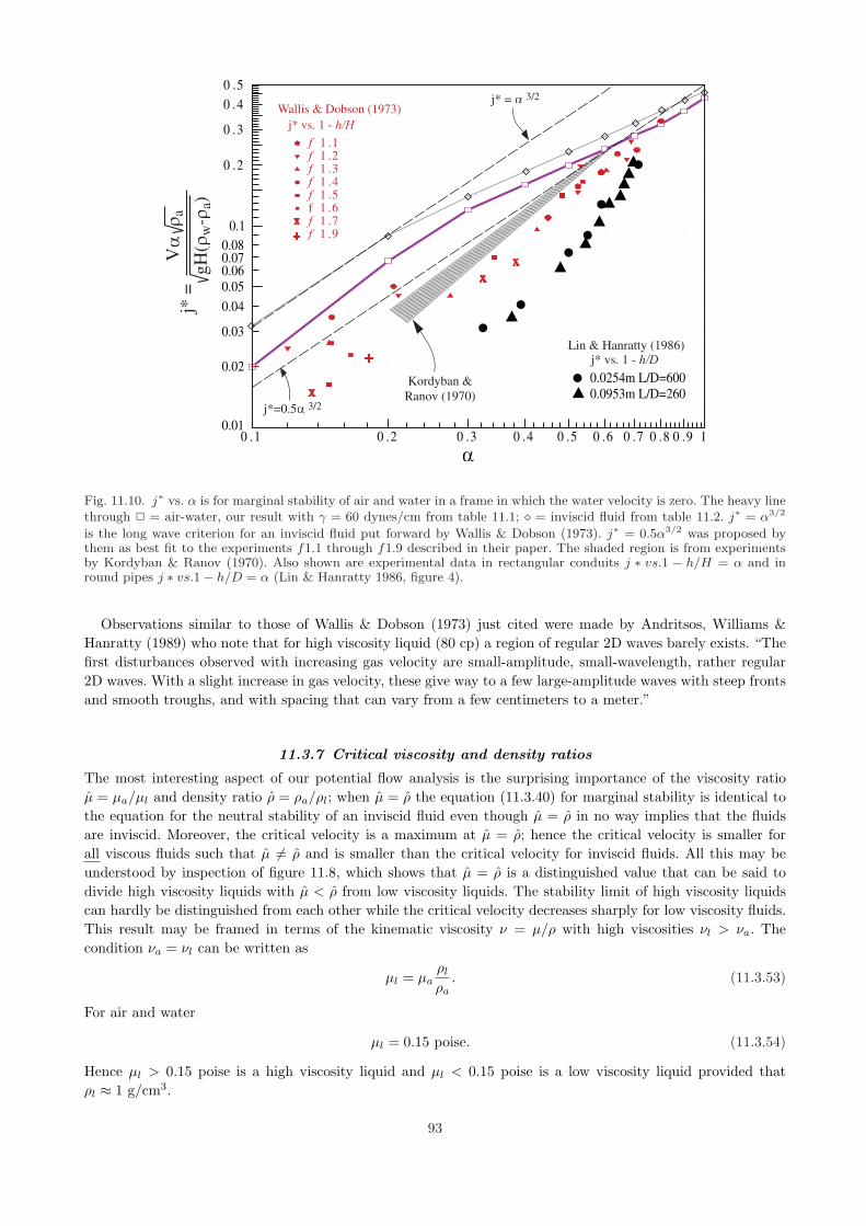
j* = a 3/2

j*=0.5a 3/2

x

x

x

+

1

f 1 .1

f 1 .2

f 1 .3

f 1 .4

f 1 .5

f 1 .6

f .7

f 1 .9

x

+

Wallis & Dobson (1973)

j* vs. 1 - h/H

0.0254m L/D=600

0.0953m L/D=260

Lin & Hanratty (1986)

Kordyban &

Ranov (1970)

j* vs. 1 - h/D

a0 .1 0 .2 0 .3 0 .4 0 .5 0 .6 0 .7 0 .8 0 .9 1

0.05

0.04

0.03

0.02

0.01

0.1

0.08

0.07

0.06

0 .2

0 .3

0 .4

0 .5

Va

ra

gH

( rw

- ra)

j* =

Fig. 11.10. j∗ vs. α is for marginal stability of air and water in a frame in which the water velocity is zero. The heavy linethrough 2 = air-water, our result with γ = 60 dynes/cm from table 11.1; ¦ = inviscid fluid from table 11.2. j∗ = α3/2

is the long wave criterion for an inviscid fluid put forward by Wallis & Dobson (1973). j∗ = 0.5α3/2 was proposed bythem as best fit to the experiments f1.1 through f1.9 described in their paper. The shaded region is from experimentsby Kordyban & Ranov (1970). Also shown are experimental data in rectangular conduits j ∗ vs.1 − h/H = α and inround pipes j ∗ vs.1− h/D = α (Lin & Hanratty 1986, figure 4).

Observations similar to those of Wallis & Dobson (1973) just cited were made by Andritsos, Williams &Hanratty (1989) who note that for high viscosity liquid (80 cp) a region of regular 2D waves barely exists. “Thefirst disturbances observed with increasing gas velocity are small-amplitude, small-wavelength, rather regular2D waves. With a slight increase in gas velocity, these give way to a few large-amplitude waves with steep frontsand smooth troughs, and with spacing that can vary from a few centimeters to a meter.”

11.3.7 Critical viscosity and density ratios

The most interesting aspect of our potential flow analysis is the surprising importance of the viscosity ratioµ = µa/µl and density ratio ρ = ρa/ρl; when µ = ρ the equation (11.3.40) for marginal stability is identical tothe equation for the neutral stability of an inviscid fluid even though µ = ρ in no way implies that the fluidsare inviscid. Moreover, the critical velocity is a maximum at µ = ρ; hence the critical velocity is smaller forall viscous fluids such that µ 6= ρ and is smaller than the critical velocity for inviscid fluids. All this may beunderstood by inspection of figure 11.8, which shows that µ = ρ is a distinguished value that can be said todivide high viscosity liquids with µ < ρ from low viscosity liquids. The stability limit of high viscosity liquidscan hardly be distinguished from each other while the critical velocity decreases sharply for low viscosity fluids.This result may be framed in terms of the kinematic viscosity ν = µ/ρ with high viscosities νl > νa. Thecondition νa = νl can be written as

µl = µaρl

ρa. (11.3.53)

For air and water

µl = 0.15 poise. (11.3.54)

Hence µl > 0.15 poise is a high viscosity liquid and µl < 0.15 poise is a low viscosity liquid provided thatρl ≈ 1 g/cm3.

93

Ugs (m/s )

Uls

(m

/s)

1 3 5 7 9 11 15 19 250.0001

0.0003

0.0005

0.0007

0.0009

0.002

0.004

0.006

0.0080.01

0.03

0.05

0.07

0.092.52cm, 1cP

2.52cm,16cP

2.52cm,70cP

9.53cm,1cP

9.53cm,12cP

9.53cm,80cP

Fig. 11.11. (After Andritsos & Hanratty 1987.) The borders between smooth stratified flow and disturbed flow areobserved in experiment. The water-air data is well below the cluster of high viscosity data that is bunched together.

Other authors have noted unusual relations between viscous and inviscid fluids. Barnea & Taitel (1993) notethat “the neutral stability lines obtained from the viscous Kelvin-Helmholtz analysis and the inviscid analysisare quite different for the case of low liquid viscosities, whereas they are quite similar for high viscosity, contraryto what one would expect.” Their analysis starts from a two-fluid model and it leads to different dispersionrelations; they do not obtain the critical condition µ = ρ. Earlier, Andritsos et al (1989) noted a “surprisingresult that the inviscid theory becomes more accurate as the liquid viscosity increases.”

Andritsos & Hanratty (1987) have presented flow regime maps for flows in 2.52 cm and 9.53 cm pipe forfluids of different viscosity ranging from 1 cp to 80 cp. These figures present flow boundaries; the boundaries ofinterest to us are those that separate ‘smooth’ flow from disturbed flow. Liquid holdups (essentially α) are notspecified in these experiments. We extracted the smooth flow boundaries from figures in Andritsos & Hanratty(1987) and collected them in our figure 11.11. It appears from this figure that the boundaries of smooth flowfor all the liquids with µl > 15 cp are close together, but the boundary for water with µl = 1 cp is much lower.The velocities shown in these figures are superficial velocities; the average velocities which could be comparedwith critical velocities in tables 11.1, 11.2 and 11.3 are larger than the superficial velocities and are significantlylarger than those in the tables.

Even earlier Francis (1951) had observed that even though the inviscid prediction of the KH instabilityoverestimates the onset for air over water, this prediction is in good agreement with experiments in rectangularducts when air is above water.

11.3.8 Further comparisons with previous results

In practice interest in the pipelining of gas-liquid flow is in round pipes. All experiments other than those ofKordyban & Ranov (1970) and Wallis & Dobson (1973) reviewed in section 11.3.6 have been carried out in roundpipes. To our knowledge there is no other theoretical study in which the stability of stratified flow in a roundpipe is studied without approximations. Theoretical studies of stability of stratified flow have been presentedby Wallis (1969); Wu et al. (1987), Barnea (1991), Crowley, Wallis & Barry (1992), Kordyban & Ranov (1970),Wallis & Dobson (1973), Taitel & Dukler (1976), Mishima & Ishii (1980), Lin & Hanratty (1986), Andritsos &Hanratty (1987), Andritsos et al. (1989), Barnea & Taitel (1993). Viscosity is neglected by Kordyban & Ranov

94

(1970), Wallis & Dobson (1973), Taitel & Dukler (1976) and Mishima & Ishii (1980). Surface tension is neglectedby Wallis (1969), Kordyban & Ranov (1970), Wallis & Dobson (1973), Taitel & Dukler (1976), Mishima & Ishii(1980) and Lin & Hanratty (1986). Wallis (1969), Lin & Hanratty (1986), Wu et al. (1987), Barnea (1991),Crowley et al. (1992) and Barnea & Taitel (1993) use one or other of the forms of two-fluids equations. Inthese equations averaged variables are introduced, the actual geometry is represented only so far as its area andround, elliptical or rectangular pipes with equal areas are equivalent. The effects of viscosity in these averagedmodels are introduced through empirical wall and interfacial fraction correlations. All these authors neglect thenormal component of viscous stress (extensional stresses are neglected). The approach of Andritsos & Hanratty(1987), Andritsos et al. (1989) is different; all the main physical effects are represented in analysis of the planeflow which is later applied to flow in round pipes. The disturbance equations for the liquid are solved exactlyexcept that the shear of basic liquid flow is neglected using a plug flow assumption. The effects of the gas on theliquid are represented through empirical correlations and further approximations are required for round pipes.

The viscous analysis of Andritsos & Hanratty (1987) for stability of stratified flow indicates that the criticalvelocity increases with increasing viscosity unlike the present analysis which predicts no such increase whenνl > νa. The discrepancy may be due to the approximations made by Andritsos & Hanratty (1987).

Experiments on the stability of stratified flow have been reported by Kordyban & Ranov (1970), Wallis& Dobson (1973), Taitel & Dukler (1976), Lin & Hanratty (1986), Crowley et al. (1992) and Andritsos &Hanratty (1987). The experiments of Lin & Hanratty (1986) and Andritsos & Hanratty (1987) do not havedata giving the height of the liquid and gas layers. Kordyban & Ranov (1970) and Wallis & Dobson (1973)did experiments in rectangular ducts, the geometry analysed in this paper, the other experiments were done inround pipes. Authors Lin & Hanratty (1986), Crowley et al. (1992) and Andritsos & Hanratty (1987) are theonly experimenters to report results for fluids with different viscosities.

It is difficult to compare the results of experiments in round pipes and rectangular channels. The commonpractice for round pipes is to express results in terms of h/D where D is the pipe diameter and h is the heightabove the bottom of the pipe; h/H is the liquid fraction in rectangular pipes and α = 1 − h/H is the gasfraction, but h/D is not the liquid fraction in round pipes and 1− h/D is not the gas fraction in round pipes.Lin & Hanratty (1986) presented experimental results for thin liquid films in round pipes giving (their figure 4)h/D vs. j∗; we converted their results to j∗ vs. 1−h/D and compared them in figure 11.10 with the results forrectangular pipes. The experimental results for round pipes are much lower than those for rectangular pipes.All this points to the necessity of taking care when comparing results between round and rectangular pipes andinterpreting results of analysis for one experiment to another.

In general we do not expect viscous potential flow analysis to work well in two-liquid problems; we get goodresults only when one of the fluids is a gas so that retarding effects of the second liquid can be neglected.However, the case of Holmboe waves studied by Pouliquen, Chomaz & Huerre (1994) may have a bearing on thetwo-liquid case. These waves appear only near our critical condition of equal kinematic viscosity. They accountfor viscosity by replacing the vortex sheet with layers of constant vorticity across which no-slip conditions andthe continuity of shear stress are enforced for the basic flow but the disturbance is inviscid. They did notentertain the notion that an inviscid analysis is just what would emerge from the condition of equal kinematicviscosity for viscous potential flow.

11.3.9 Nonlinear effects

None of the theories agree with experiments. Attempts to represent the effects of viscosity are only partial, asin our theory of viscous potential flow, or they require empirical data on wall and interfacial friction, which arenot known exactly and may be adjusted to fit the data. Some choices for empirical inputs underpredict andothers overpredict the experimental data.

It is widely acknowledged that nonlinear effects at play in the transition from stratified to slug flow are notwell understood. The well-known criterion of Taitel & Dukler (1976), based on a heuristic adjustment of thelinear inviscid long wave theory for nonlinear effects, is possibly the most accurate predictor of experiments.Their criterion replaces j∗ = α3/2 with j∗ = α5/2. We can obtain the same heuristic adjustment for nonlineareffects on viscous potential flow by multiplying the critical value of velocity in table 11.1 by α. Plots of j∗ = α3/2,j∗ = α5/2 and the heuristic adjustment of viscous potential flow, together with the experimental values of Wallis& Dobson (1973) and Kordyban & Ranov (1970) are shown in figure 11.13. The good agreement in evidencethere lacks a convincing foundation.

95

Fig. 11.12. Local liquid velocity UL versus local gas velocity UG for PDVSA-Intevep data from 0.508 m i.d. flow loopwith air and 0.404 Pa s lube oil. The identified flow patterns are SS (open circles), SW (open squares). Straftified tonon-stratified flow transition theories after different authors are compared; TD: stars, BT: +, FJ: broken line, Funadaand Joseph multiplied by α (2001) FJ ×α heavy line. Constant void fraction α lines are indicated. Notice that the curvesFJ and FJ ×α sharply drop around UB5 m/s, separating SS data from SW data.

To summarize, we studied Kelvin-Helmholtz stability of superposed uniform streams in rectangular ductsusing viscous potential flow. Viscous potential flows satisfy the Navier-Stokes equations. Because the no-slipcondition can not be satisfied the effects of shear stresses are neglected, but the effects of extensional stresses atthe interface on the normal stresses are fully represented. The solution presented is complete and mathematicallyrigorous. The effects of shear stresses are neglected at the outset; after that no empirical inputs are introduced.The main result of the analysis is the emergence of a critical value of velocity, discussed in section 11.3.7.The main consequence of this result is that for air-liquid systems the critical values of velocity for liquids withviscosities greater than 15 cp are essentially independent of viscosity and the same as for an inviscid fluid, but forliquids with viscosities less than 15 cp the stability limits are much lower. The criterion for stability of stratifiedflow given by viscous potential flow is in good agreement with experiments when the liquid layer is thin, but itoverpredicts the data when the liquid layer is thick. Though viscous potential flow neglects the effects of shearthe qualitative prediction of the peculiar effects of liquid viscosity has been obtained by other authors usingother methods of analysis in which shear is not neglected. A rather accurate predictor of experimental resultsis given by applying the Taitel & Dukler nonlinear correction factor to account for the effect of finite amplitudewave on the results of viscous potential flow.

11.3.10 Combinations of Rayleigh-Taylor and Kelvin-Helmholtz instabilities

Dispersion relations for the combined action of RT and KH instability of irrotational flows of inviscid fluids arepresented in the first chapter of the book by Drazin and Reid 1981.

The analysis of the combined action of RT and KH instability can be readily extended to include importanteffects of viscosity in irrotational flows by techniques explained in Chapter 9 and 11. Updating the potentialflow analysis of the dispersion relation to include effects of viscosity using VPF is very easily done and theresults are only marginally more complicated than those given by the inviscid analysis but with a much richerphysical content.

The extension of nonlinear analysis based on potential flow of inviscid fluids can also be extended to findthe irrotational effects of viscosity. The combination of the two instabilities is ubiquitous in nonlinear problems.Joseph, Liao and Saut (1992) considered the KH mechanism for side branching in the displacement of lightwith heavy fluid under gravity. They showed that the strongest Hadamard instabilities occur as KH instabilities

96

X

X

XX

+

x

xx

x

x

x

x

a

j*

0 .1 0 .2 0 .3 0 .4 0 .5 0 .6 0 .7 0 .8 0 .9 1

0 .0 5

0 .1

0 .1 5

0 .2

0 .2 5

0 .3

0 .3 5

0 .40 .4 5

0 .5

j* = a 3/2

[WD] Theory

j*=0.5a 3/2

[WD] Best fit

j* = a 5/2

[TD]

VPF: Table 1 with

critical values

reduced by factor a

[TD]

Fig. 11.13. Nonlinear effects. The Taitel-Dukler 1976 correction (multiply by α).

Fig. 11.14. (Varga et al. 2003) Schematic of the development of the liquid jet breakup process.

associated with a velocity difference at the sides of falling fingers. The Hadamard instabilities will be regularizedby adding irrotational effects of viscosity and surface tension.

Another example of combined KH-RT instability goes in another way. Instead of generating a secondary KHinstability on a primary RT instability generated by falling fingers, a secondary RT instability can develop ona primary KH instability in a small-diameter liquid jet exposed to a large-diameter high-speed gas jet studiedby Varga, Lasheras and Hopfinger 2003. They proposed a breakup model based on the acceleration mechanismwhich breakup liquid drops in a high speed air stream studied in chapter 9. In their model, the RT instabilityis generated on the wave crests generated by a primary KH instability, as is shown in figures 11.14-11.17.

Varga et al. 2003 show that the mean droplet sizes scale well on the most unstable RT wavelength. Thedependence of the droplet diameter on both the atomizing gas velocity and the liquid surface tension aresuccessfully captured by the proposed breakup model.

97

Fig. 11.15. (Varga et al. 2003) Sketch of the gas and liquid streamlines in the liquid tongue formation process.

Fig. 11.16. (Varga et al. 2003) Instantaneous flow image with identified Rayleigh-Taylor wavelengths, Dl =0.32 mm,We =37, λmeasured = 200µm. (cf. figures 9.6-9.8)

Fig. 11.17. (Varga et al. 2003) Instantaneous flow image with identified Rayleigh-Taylor wavelengths, Dl =0.32 mm,We =47, λmeasured = 185µm. (cf. Figs. 9.6-9.8)

98

12

Energy equation for irrotational theories ofgas-liquid flow: viscous potential flow (VPF),

viscous potential flow with pressurecorrection (VCVPF), dissipation method

(DM)

12.1 Viscous potential flow (VPF)

The effects of viscosity on the irrotational motions of spherical cap bubble, Taylor bubbles in round tubes,Rayleigh-Taylor and Kelvin-Helmholtz instability described in previous chapters were obtained by evaluatingthe viscous normal stress on potential flow. In gas-liquid flows, the viscous normal stress does not vanish and itcan be evaluated on the potential. It can be said that in the case of gas-liquid flow, the appropriate formulationof the irrotational problem is the same as the conventional one for inviscid fluids with the caveat that the viscousnormal stress is included in the normal stress balance. This formulation of viscous potential flow is not at allsubtle; it is the natural and obvious way to express the equations of balance when the flow is irrotational andthe fluid viscous.

We shall use the acronym VPF, viscous potential flow, to stand for the irrotational theory in which theviscous normal stresses are evaluated on the potential.

In gas-liquid flows we may assume that the shear stress in the gas is negligible so that no condition need beenforced on the tangential velocity at the free surface, but the shear stress must be zero. The condition that theshear stress is zero at each point on the free surface is dropped in the irrotational approximations. In general,you get an irrotational shear stress from the irrotational analysis. The discrepancy between this shear stressand the zero shear stress required for exact solutions will generate a vorticity layer. In many cases this layer isthin and its influence on the bulk motion and on the irrotational effects of viscosity is minor. Exact solutionscannot be the same as any irrotational approximation for cases in which the irrotational shear stress does notvanish.

12.2 Dissipation method according to Lamb

Another purely irrotational theory of flow of viscous fluids is associated with the dissipation method. Theacronym DM is used for the dissipation method. The DM extracts information from evaluating the equationgoverning the evolution of energy and dissipation on irrotational flow. VPF does not rely on arguments aboutenergy and dissipation and the results of the two irrotational theories, DM and VPF, are usually different.

The dissipation method was used by Lamb (1932) to compute the decay of irrotational waves due to viscosity.This method can be traced back to Stokes (1851). A pressure correction was not introduced in these studies.Lamb presented some exact solutions from which the irrotational approximation can be evaluated and the natureof the boundary layer rigorously examined. Lamb (1932) studied the viscous decay of free oscillatory waves ondeep water § 348 and small oscillations of a mass of liquid about the spherical form § 355, using the dissipationmethod. Lamb showed that in these cases the rate of dissipation can be calculated with sufficient accuracy byregarding the motion as irrotational.

Lamb’s (1932) calculations are based on the assumption that the speed of a progressive wave is the sameas in an inviscid fluid. Padrino (Padrino and Joseph 2006, §14.2.4 and 14.3.1) noticed that a more completecalculation of the dissipation method yields a different result; the growth rates are the same as in Lamb’scalculation but the speed of the wave depends on the viscosity of the liquid.

99

12.3 Drag on a spherical gas bubble calculated from the viscous dissipation of an irrotationalflow

The computation of the drag D on a sphere in potential flow using the dissipation method seems to have beengiven first by Bateman in 1932 (see Dryden, Murnaghan, and Bateman 1956) and repeated by Ackeret (1952).They found that D = 12πaµU where µ is the viscosity, a radius of the sphere and U its velocity. This drag istwice the Stokes drag and is in better agreement with the measured drag for Reynolds numbers in excess ofabout 8.

The drag on a spherical gas bubble of radius a rising in a viscous liquid at modestly high Reynolds numberswas calculated, using the dissipation method by various investigators beginning with Levich (1949), who obtainedthe value 12πaµU or equivalently the drag coefficient 48/R, where R = 2aUρ/µ is the Reynolds number, bycalculating the dissipation of the irrotational flow around the bubble. Moore (1959) calculated the drag directlyby integrating the pressure and viscous normal stress of the potential flow and neglecting the viscous shearstress (which physically should be zero), obtaining the value 8πaµU .

12.4 The idea of a pressure correction

The discrepancy between the two drag values led G. K. Batchelor, as reported by Moore (1963), to suggestthe idea discrepancy could be resolved by introducing a viscous correction to the irrotational pressure. We donot know whether we should praise or blame Batchelor for this idea since it comes to us second hand. Thereis no doubt that the pressure in the liquid depends on the viscosity and it could take on its largest values inboundary layer next to the free surface but the velocity there could also come to depend on the viscosity. Moore(1963) performed a boundary layer analysis and his pressure correction is readily obtained by setting y = 0 inhis equation (2.37):

pv = (4/R) (1− cos θ)2 (2 + cos θ) / sin2 θ (12.4.1)

which is singular at the separation point where θ = π. The presence of separation is a problem for the applicationof boundary layers to the calculation of drag on solid bodies. To find the drag coefficient Moore (1963) calculatedthe momentum defect, and obtained the Levich value 48/R plus contributions of order R−3/2 or lower.

Kang & Leal (1988a, b) put the shear stress of the potential flow on the bubble surface to zero and calcu-lated a pressure correction. They obtained the drag coefficient given by Levich’s dissipation approximation bydirect integration of the normal viscous stress and pressure over the bubble surface. They accomplished this byexpanding the pressure correction as a spherical harmonic series and noting that only one term of this seriescontributes to the drag, no appeal to the boundary-layer approximation being necessary. A similar result wasobtained by Joseph & Wang (2004a) using their theory described below, for computing a pressure correction.

The accepted idea, starting with Batchelor, is that the pressure correction is a real viscous pressure whichvaries from the pressure in the irrotational flow outside a narrow vorticity layer near the gas-liquid surface, tothe required value at the interface. This boundary layer has not been computed. Maybe the idea is not quitecorrect. In the case of the decay of free irrotational gravity waves computed by Lamb (1932), a viscous pressurecorrection does not appear. The pressure correction computed by Wang & Joseph (2006d) as shown in §14.1gives the same result as the dissipation method and is in excellent agreement with the exact solution but it isnot a viscous correction in a boundary layer of the exact solution.

12.5 Energy equation for irrotational flow of a viscous fluid

Consider the equations of motion for an incompressible Newtonian fluid with gravity as a body force per unitmass

ρdudt

= −∇Φ + µ∇2u (12.5.1)

where

Φ = p + ρgz. (12.5.2)

The stress is given by

T = −p1 + τ (12.5.3)

100

where

τ = 2µD[u]

and

∇ · τ = µ∇2u

The mechanical energy equation corresponding to (12.5.1) is given by

ddt

∫

Ω

ρ

2|u|2 dΩ =

∫

S

n · T · udS − 2µ

∫

Ω

D : D dΩ, (12.5.4)

where S is the boundary of Ω, with outward normal n. On solid boundaries no-slip is imposed; say u = 0 there,and on the free surface

z = η(x, y, t)

and the shear stress

n ·T · es = 0, (12.5.5)

where es is any vector tangent to the free surface Sf . On Sf we have∫

S

n · T · udS =∫

Sf

n · T · udS

where

T = T− ρgη1, (12.5.6)

n ·T · n = −γ∇II · n. (12.5.7)

Hence, on Sf

n · T · n = −ρgη − γ∇II · n. (12.5.8)

and, since the shear stress vanishes on Sf

n · T · u = n · T · (unn + uses)

= −(ρgη + γ∇II · n)un. (12.5.9)

Hence, (12.5.4) may be written as

ddt

∫

Ω

ρ

2|u|2 dΩ = −

∫

Sf

(ρgη + γ∇II · n)undSf − 2µ

∫

Ω

D : D dΩ, (12.5.10)

Equation (12.5.10) holds for viscous fluids satisfying the Navier–Stokes equations (12.5.1) subject to the van-ishing shear stress condition (12.5.5).

We turn now to potential flow u = ∇φ, ∇2φ = 0. In this case, ∇2u = 0 but the dissipation does not vanish.How can this be? In Chapter 4 we showed that the irrotational viscous stress is self-equilibrated and does giverise to a force density term ∇2∇φ = 0; however, the power of self-equilibrated irrotational viscous stresses

∫

Sf

n · 2µ∇⊗∇φ · udSf

does not vanish, and it gives rise to an irrotational viscous dissipation

2µ

∫

Ω

D[u] : D[u]dΩ = 2µ∫

Ω

∂2φ

∂xi∂xj

∂2φ

∂xi∂xjdΩ = 2µ

∫

S

nj∂2φ

∂xj∂xiuidS

= 2µ

∫

Sf

n ·D[∇φ] · udSf = 2µ

∫

Sf

n ·D · (unn + uses) dSf

=∫

Sf

(2µ

∂2φ

∂n2un + τsus

)dSf (12.5.11)

101

where τs is an irrotational shear stress

τs = 2µn ·D[∇φ] · es,

us = u · es. (12.5.12)

Turning next to the inertial terms, we have

(u · ∇)u = ∇|u|2

2

and

ddt

∫

Ω

ρ

2|u|2dΩ =

∫

Ω

ρ

(u · ∂u

∂t+ u · ∇|u|

2

2

)dΩ

=∫

Ω

ρ

[∂φ

∂xi

∂

∂xi

∂φ

∂t+∇ ·

(u|u|22

)]dΩ

=∫

Sf

ρun

(∂φ

∂t+|∇φ|2

2

)dSf (12.5.13)

Collecting the results (12.5.9), (12.5.11), (12.5.12) and (12.5.13) we need to evaluate the energy equation (12.5.4)for (12.5.1) when u = ∇φ; we find that

∫

Sf

un

[ρ

(∂φ

∂t+|∇φ|2

2+ gη

)+ 2µ

∂2φ

∂n2+ γ∇II · n

]dSf = −

∫

Sf

τsusdSf . (12.5.14)

Equation (12.5.14) was derived by Joseph; it is the energy equation for the irrotational flow of a viscous fluid.As in the case of the radial motion of a spherical gas bubble (6.0.8), the normal stress balance converts into theenergy equation for viscous irrotational flow.

12.6 Viscous correction of viscous potential flow

The viscous pressure pv for VCVPF can be defined by the equation∫

Sf

(−pv)undSf =∫

Sf

τsusdSf . (12.6.1)

This equation can be said to arise from the condition that the shear stress should vanish but it does not vanishin the irrotational approximation. Batchelor’s idea, as reported by Moore (1963), is that the additional drag4πaµU on a spherical gas-bubble needed to obtain the Levich drag 12πaµU from the value 8πaµU , computedusing the viscous normal stress, arises from a real viscous pressure in a thin boundary layer at the surface ofthe bubble.

Our interpretation of Batchelor’s idea is to replace the unwanted shear stress term in the energy equationwith an additional contribution to the normal stress in the form of a viscous pressure satisfying (12.6.1). Anidentical interpretation of Batchelor’s idea, with a different implementation, has been proposed by Kang andLeal (1988b) and is discussed in §13.1.1.

Suppose now that there is such a pressure correction and Bernoulli equation

pi + ρ

(∂φ

∂t+|∇φ|2

2+ gη

)= C

holds. Since

C

∫

S

u · ndS = C

∫

Ω

∇ · udΩ = 0

we obtain∫

Sf

un

[−pi − pv + 2µ

∂2φ

∂n2+ γ∇II · n

]dSf = 0 (12.6.2)

The normal stress balance for VCVPF is

− pi − pv + 2µ∂2φ

∂n2+ γ∇II · n = 0 (12.6.3)

102

Equation (12.6.3) is a working equation in the VCVPF theory only if pv can be calculated. In the problemsdiscussed in this book, pv and a velocity correction uv are coupled in a linear equation

ρ∂uv

∂t= −∇pv + µ∇2uv, ∇ · uv = 0, (12.6.4)

and since uv is harmonic ∇2pv = 0 and pv can be represented by a series of harmonics functions. In most ofthe problems in this book, orthogonality conditions show that all the terms in the series but one are zero andthis one term is completely determined by (12.6.1). In other problems, such as the flow over bodies studied inChapter 13, (12.6.1) determines the coefficient of the term in the harmonic series that enters into the directcalculation of the drag; the other coefficients remain undetermined.

Having obtained pv it is necessary to consider the problem (12.6.4) for uv. This problem is overdetermined;(12.6.4) is a system of four equations for three unknowns. We must also satisfy the kinematic equation uv =∂ηv/∂t and the normal stress boundary condition. Wang and Joseph (2006d) showed that a purely irrotationaluv and higher order corrections satisfaying (12.6.1) can be computed in the case in which the normal stressbpundary condition is not corrected. Their solution procedure leads to a series of purely irrotational velocitiesin powers of ν, or reciprocal powers of the Reynolds number (see §14.12). This same kind of special irrotationalsolution in reciprocal powers of the Reynolds number was constructed by Funada et al (2005) for capillaryinstability of a viscous fluid and by Wang et al (2005b) for a capillary instability of a viscoelastic fluid.

There is no reason to think that the higher order irrotational solutions generated by pv have a hydrodynamicalsignificance. In general, the solution of potential flow problems with pressure corrections can be expected toinduce vorticity. This is the case for the nonlinear model of capillary collapse and rupture studied in §17.4.2. Theflow from irrotational stagnation points of depletion to irrotational stagnation points of accumulation cannotoccur without generating the vorticity given by (17.4.24) at leading order.

In the direct applications of the dissipation method, a pressure correction is not introduced; the power of theirrotational shear stress on the right side of (12.5.14) is computed directly. The energy equation for the systemof VCVPF equations with pv is the same as (12.5.14) when the power of pv is replaced by the power of theshear stress using (12.6.1).

In the case of rising bubbles we may compute the same value for the drag in a direct computation in whichthe irrotational shear stress is neglected and pv is included as we get from the dissipation method using (12.5.14)with τs 6= 0 and pv = 0.

The dissipation method requires that we work with the power generated by the shear usτs and not with adirect computation using pv. The direct computation of drag with pv = 0 and τs 6= 0 given by potential flowleads to zero drag (13.1.8). The pressure correction allows us to do direct calculations without using the energyequations. The two methods lead to the same results by different routes. This feature of energy analysis isrelated to the fact that irrotational stresses are self-equilibrated (4.3.1) but do work.

The nature of the construction of VCVPF equations, which have the same energy equations as those used inthe dissipation method, guarantees that the same results will be obtained by these two methods.

The VCVPF theory is perhaps artificial in some cases, like the decay of gravity waves in which no viscouspressure appears in the exact solution (see §14.1.3). However, in all cases, VCVPF leads to the same results asthe dissipation method.

We have now arrived at the following classification of irrotational solutions:IPF - inviscid potential flowVPF - viscous potential flowVCVPF - viscous correction of viscous potential flowDM - dissipation methodRecognizing now that DM and VCVPF lead to the same results by different routes, even if pv is not a true

hydrodynamic pressure, we can introduce yet another acronymVCVPF/DMandES - exact solution.VCVPF/DM and VPF are different irrotational solutions; they give rise to different results in nearly every

instance except in the case of the limit of very high Reynolds numbers where they tend to the inviscid limitIPF. At finite Reynolds number VPF and VCVPF/DM can give significantly better results, closer to the exactsolutions than IPF.

103

In the sequel, VCVPF means VCVPF/DM. We think that it is possible that either VPF or VCVPF give(in different situations which we presently cannot specify a priori with precision) the best possible purelyirrotational approximations to the exact solution. The problem of the best purely irrotational approximationof real flows is related to the problem of the optimal specification of the irrotational flow in the Helmholtzdecomposition studied in Chapter 4.

104