
Potential Difference Potential Field Potential Gradient...
28
Indraprastha Institute of Information Technology Delhi ECE230 Lecture – 12 Date: 03.02.2014 • Potential Difference • Potential Field • Potential Gradient • Electric Dipole
Transcript of Potential Difference Potential Field Potential Gradient...

Indraprastha Institute of
Information Technology Delhi ECE230
Lecture – 12 Date: 03.02.2014 • Potential Difference • Potential Field • Potential Gradient • Electric Dipole

Indraprastha Institute of
Information Technology Delhi ECE230
• Say A and B are two points somewhere on a circuit. But let’s call these points something different, say point + and point - .
(r).C
V E dl + -
• V represents the potential difference (in volts) between point (i.e., node) + and point (node) - . Note this value can be either positive or negative.
Q: But, does this mean that circuits produce electric fields?
Potential Difference

Indraprastha Institute of
Information Technology Delhi ECE230
A: Absolutely! Anytime you can measure a voltage (i.e., a potential difference) between two points, an
electric field must be present!
Potential Difference (contd.)

Indraprastha Institute of
Information Technology Delhi ECE230
Potential Difference (contd.)
• Note that VAB can be expressed as:
(r). (r ) (r )AB A B
C
V E dl V V
where point A lies at the beginning of contour C, and B
lies at the end.
• The potential at any point is the potential difference between that point and a chosen point (or reference point) at which the potential is zero (usually ground !).
( ).
r
V E r dl
Indraprastha Institute of
Information Technology Delhi ECE230
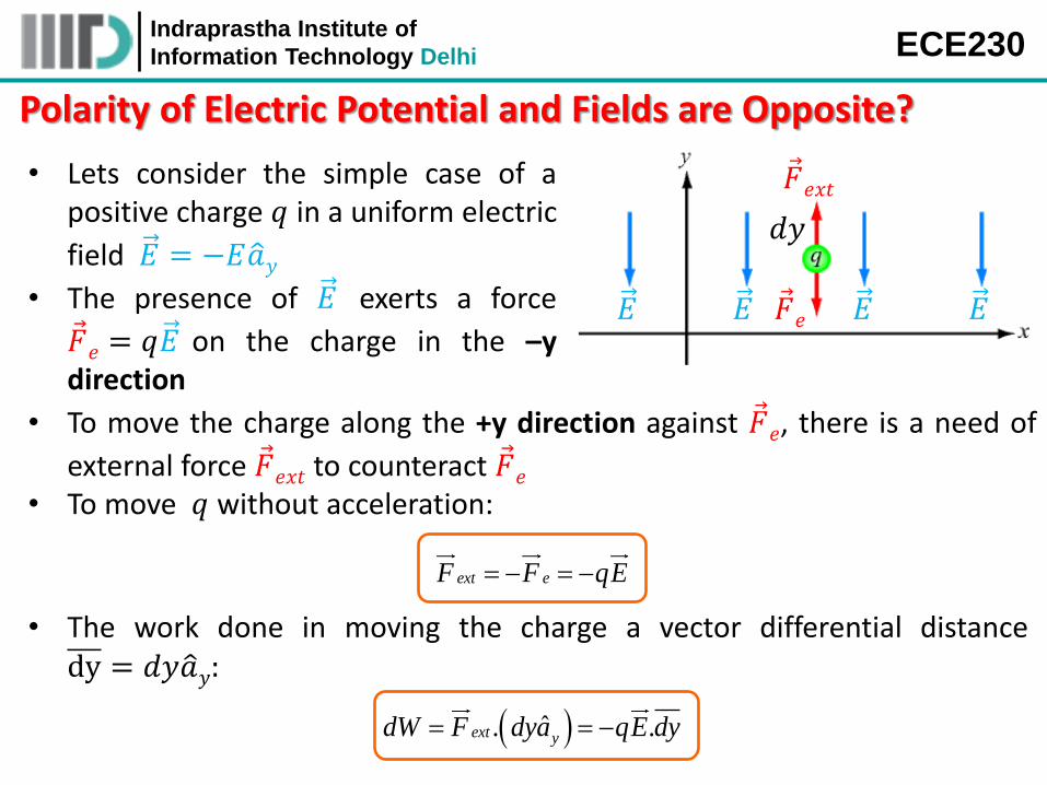
Polarity of Electric Potential and Fields are Opposite?
𝐸 𝐸 𝐸 𝐸
• Lets consider the simple case of a positive charge 𝑞 in a uniform electric
field 𝐸 = −𝐸𝑎 𝑦
• The presence of 𝐸 exerts a force
𝐹 𝑒 = 𝑞𝐸 on the charge in the –y direction
𝐹 𝑒
• To move the charge along the +y direction against 𝐹 𝑒, there is a need of
external force 𝐹 𝑒𝑥𝑡 to counteract 𝐹 𝑒 • To move 𝑞 without acceleration:
𝐹 𝑒𝑥𝑡
ext eF F qE
• The work done in moving the charge a vector differential distance dy = 𝑑𝑦𝑎 𝑦:
𝑑𝑦
ˆ. .ext ydW F dya qE dy

Indraprastha Institute of
Information Technology Delhi ECE230
Polarity of Electric Potential and Fields are Opposite?
• Now, the electric potential is the energy per unit charge:
dWdV
q .dV E dy
Conclusion of our Premise !
Indraprastha Institute of
Information Technology Delhi ECE230
Electric Potential for Point Charge
• Recall that a point charge Q, located at the origin ((𝑟′ = 0), produces a static electric field:
• Now, we know that this field is the gradient of some scalar field:
Q: What is the electric potential function V(𝑟 ) generated by a point charge Q, located at the origin?
Q: Where did this come from ? How do we know that this is the correct solution? A: We can show it is the correct solution by direct substitution!
2
0
ˆ(r)4
r
QE a
r
(r) ( )E V r
A: We find that it is: 0
(r)4
QV
r

Indraprastha Institute of
Information Technology Delhi ECE230
(r) ( )E V r 04
Q
r
'
0
ˆ 0 04
r
Qa
r r
The correct result!
Q: What if the charge is not located at the origin ? A: Substitute r with |𝑟 − 𝑟′ |, and we get:
Electric Potential for Point Charge (contd.)
Verification:
2
0
ˆ(r) ( )4
r
QE V r a
r
0
(r)4 '
QV
r r
where, as before, the position vector 𝑟′ denotes the location of the charge Q, and the position vector 𝑟 denotes the location in space
where the electric potential function is evaluated.

Indraprastha Institute of
Information Technology Delhi ECE230
• The scalar function V(𝑟 ) for a point charge can be shown graphically as a contour plot:
Electric Potential for Point Charge (contd.)
Indraprastha Institute of
Information Technology Delhi ECE230
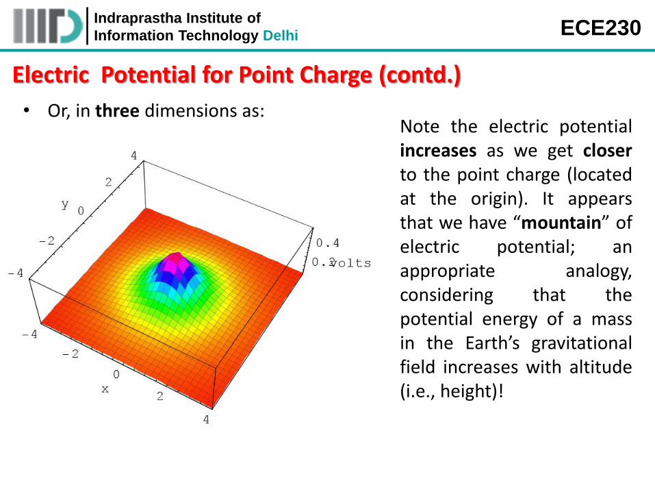
Electric Potential for Point Charge (contd.)
• Or, in three dimensions as: Note the electric potential increases as we get closer to the point charge (located at the origin). It appears that we have “mountain” of electric potential; an appropriate analogy, considering that the potential energy of a mass in the Earth’s gravitational field increases with altitude (i.e., height)!

Indraprastha Institute of
Information Technology Delhi ECE230
Electric Potential for Point Charge (contd.)
• Recall the electric field produced by a point charge is a vector field that looks like:

Indraprastha Institute of
Information Technology Delhi ECE230
• Combining the electric field plot with the electric potential plot, we get:
Electric Potential for Point Charge (contd.)
Given our understanding of the gradient, the above
plot makes perfect sense! Do you see why ?

Indraprastha Institute of
Information Technology Delhi ECE230
Electric Potential Function for Charge Densities
• Recall the total static electric field produced by 2 different charges (or charge densities) is just the vector sum of the fields produced by each:
• Since the fields are conservative, we can write this as:
1 2(r) (r) (r)E E E
1 2(r) (r) (r)E E E 1 2( ) ( ) ( )V r V r V r
1 2( ) ( ) ( )V r V r V r
• Therefore, we find: 1 2( ) ( ) ( )V r V r V r
In other words, superposition also holds for the electric potential function! The total electric potential field produced by a collection of charges is
simply the sum of the electric potential produced by each.

Indraprastha Institute of
Information Technology Delhi ECE230
• Consider now some distribution of charge, ρ𝑣(𝑟 ). The amount of charge
dQ, contained within small volume dv, located at position 𝑟′ , is:
• The electric potential function produced by this charge is therefore:
• Therefore, integrating across all the charge in some volume v, we get:
Electric Potential Function for Charge Densities (contd.)
( ') 'vdQ r dv
0 0
( ') '( )
4 ' 4 '
vdQ r dvdV r
r r r r
0
( ')( ) '
4 '
v
v
rV r dv
r r

Indraprastha Institute of
Information Technology Delhi ECE230
• Likewise, for surface or line charge density:
Electric Potential Function for Charge Densities (contd.)
0
( ')( ) '
4 '
S
S
rV r dS
r r
0
( ')( ) '
4 '
l
C
rV r dl
r r
Note that these integrations are scalar integrations—typically they are easier to evaluate than the integrations resulting from
Coulomb’s Law.
• Once we find the electric potential function V 𝑟 , we can then determine the total electric field by taking the gradient:
(r) ( )E V r

Indraprastha Institute of
Information Technology Delhi ECE230
• Thus, we now have three (!) potential methods for determining the electric field produced by some charge distribution ρ𝑣(𝑟 ).
1. Determine 𝐸 𝑟 from Coulomb’s Law.
2. If ρ𝑣(𝑟 ) is symmetric, determine 𝐸 𝑟 from Gauss’s Law. 3. Determine the electric potential function V 𝑟 , and then determine
the electric field as 𝐸 𝑟 = −∇V(𝑟 ).
Q: Yikes! Which of the three should we use?? A: To a certain extent, it does not matter! All three will provide the same result (although ρ𝑣(𝑟 ) must be symmetric to use method 2!).
Electric Potential Function for Charge Densities (contd.)
However, if the charge density is symmetric, we will find that using Gauss’s Law (method 2) will typically result in much less work!
Otherwise (i.e., for non-symmetric ρ𝑣(𝑟 )), we find that sometimes method 1 is easiest, but in other cases method 3 is a bit less stressful
(i.e., you decide!).

Indraprastha Institute of
Information Technology Delhi ECE230
Example – 1
• Determine the electric potential at the origin due to four 20-mC charges residing in free space at the corners of a 2𝑚 × 2𝑚 square centered about the origin in the x–y plane.
• For four identical charges all equidistant from the origin:
' 2R r r m
6 5
00
4 20 10 2 10( )
4 2V r
(V)
0
4( )
4
QV r
R
Indraprastha Institute of
Information Technology Delhi ECE230
Example – 2
• A spherical shell of radius R has a uniform surface charge density ρS. Determine the electric potential at the center of the shell.
2
0 0
( ) 44
S S RV r R
R
0
( ')( ) '
4 '
S
S
rV r dS
r r
0
'( )
4 '
S
S
dSV r
r r
0
( ) '4
S
S
V r dSR

Indraprastha Institute of
Information Technology Delhi ECE230
Relationship between 𝑬 and V
• We have learnt that the electrostatic field is conservative and therefore, following is true for the given situation:
BA ABV V . 0BA AB
L
V V E dl
Line integral of 𝐸along a closed path is zero
• Lets apply Stoke’s theorem: . 0 .L S
E dl E dS 0E
Conservative or Irrotational

Indraprastha Institute of
Information Technology Delhi ECE230
Relationship between 𝑬 and V (contd.)
0E . 0BA AB
L
V V E dl
• We defined potential as: .V E dl .dV E dl
x y zdV E dx E dy E dz
• Alternatively we can also write: V V VdV dx dy dz
x y z
• Comparison gives: x
VE
x
y
VE
y
z
VE
z
• Therefore: E V
Maxwell’s equations for Electrostatics Intergal Form
Differential Form

Indraprastha Institute of
Information Technology Delhi ECE230
Relationship between 𝑬 and V (contd.)
E V
The electric field intensity is the gradient of 𝑉. The
negative sign shows that the direction of 𝐸 is opposite to
the direction in which V increases ↔ 𝐸 is directed from higher to lower levels of V
It provides another tool to determine electric field apart from Coulomb’s
and Gauss’s laws → 𝐸 can be obtained if the scalar function V is known
Indraprastha Institute of
Information Technology Delhi ECE230
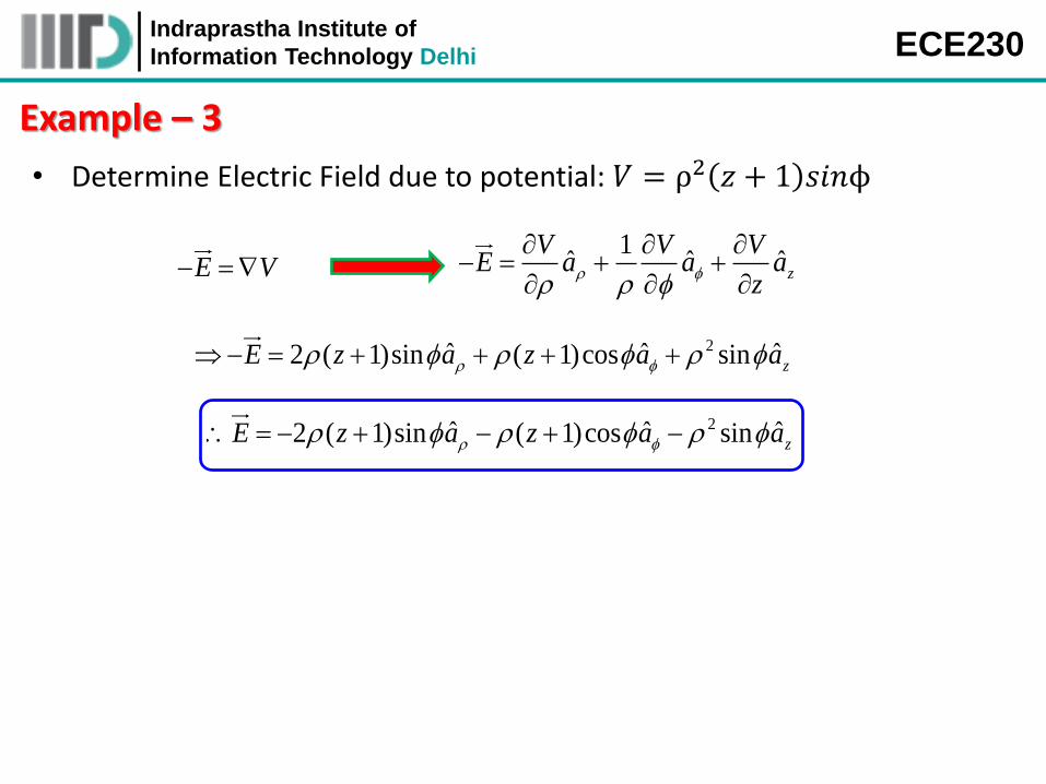
Example – 3
• Determine Electric Field due to potential: 𝑉 = ρ2 𝑧 + 1 𝑠𝑖𝑛ϕ
E V 1
ˆ ˆ ˆz
V V VE a a a
z
2ˆ ˆ ˆ2 ( 1)sin ( 1)cos sin zE z a z a a
2ˆ ˆ ˆ2 ( 1)sin ( 1)cos sin zE z a z a a

Indraprastha Institute of
Information Technology Delhi ECE230
Example – 4
• Determine Electric Field due to potential: 𝑉 = 𝑒−𝑟𝑠𝑖𝑛θ𝑐𝑜𝑠2ϕ
E V 1 1
ˆ ˆ ˆsin
r
V V VE a a a
r r r
1ˆ ˆ ˆsin cos2 cos cos2 ( 2sin 2 )
rr r
r
eE e a e a a
r r
1 2ˆ ˆ ˆsin cos2 cos cos2 sin 2
rr r
r
eE e a e a a
r r

Indraprastha Institute of
Information Technology Delhi ECE230
Poisson’s and Laplace’s Equation
• From Gauss’s Law: 0
. vE
E V • We have:
0
. vV
2 2 22
2 2 2
0
vV V VV
x y z
(Poisson’s Equation)
• If the medium under consideration contains no charge then: 2 0V
Laplace’s Equations
These formulations are extremely useful for determining the electrostatic potential V in regions with boundaries on which V is known, such as the
regions between the plates of a capacitor with specified voltage difference across it.

Indraprastha Institute of
Information Technology Delhi ECE230
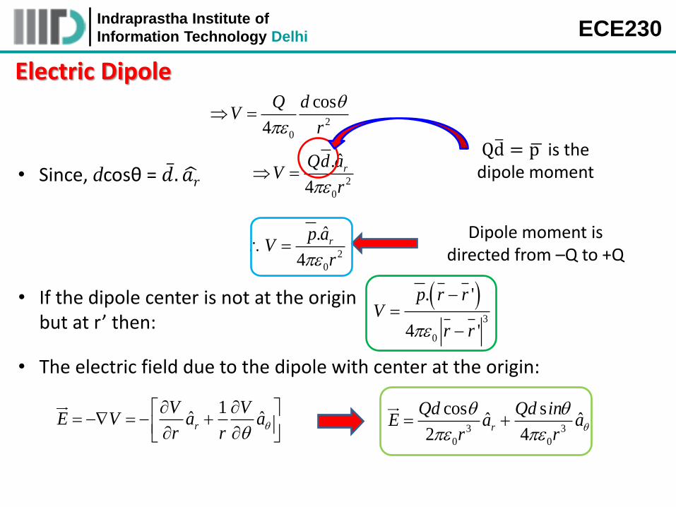
Electric Dipole
• An electric dipole is formed when two point charges of equal magnitude but opposite signs are separated by a small distance → a pretty useful configuration!!!
• In practical situation, the distance from the point of interest is much greater than the separation.
• The potential at point 𝑃(𝑟, θ, ϕ) is: P
+Q
-Q
r1
rr2
cos
2
d
za
d
• Since 𝑟 ≫ 𝑑; r, r1, and r2 are almost parallel.
2 1
0 1 2 0 1 2
1 1
4 4
Q Q r rV
r r r r
1 cos2
dr r 2 cos
2
dr r
2 1 cosr r d
2
1 2r r r• Furthermore:
Indraprastha Institute of
Information Technology Delhi ECE230
Electric Dipole
2
0
cos
4
Q dV
r
• Since, dcosθ = 𝑑 . 𝑎𝑟 2
0
ˆ.
4
rQd aV
r
Qd = p is the dipole moment
Dipole moment is directed from –Q to +Q
• If the dipole center is not at the origin but at r’ then:
• The electric field due to the dipole with center at the origin:
1ˆ ˆ
r
V VE V a a
r r
2
0
ˆ.
4
rp aV
r
3
0
. '
4 '
p r rV
r r
3 3
0 0
cos sˆ ˆ
2 4r
Qd Qd inE a a
r r
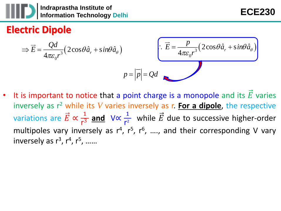
Indraprastha Institute of
Information Technology Delhi ECE230
3
0
ˆ ˆ2cos s4
r
QdE a in a
r
• It is important to notice that a point charge is a monopole and its 𝐸 varies inversely as r2 while its V varies inversely as r. For a dipole, the respective
variations are 𝐸 ∝1
r3 and V∝
1
r2 while 𝐸 due to successive higher-order
multipoles vary inversely as r4, r5, r6, …., and their corresponding V vary inversely as r3, r4, r5, ……
Electric Dipole
3
0
ˆ ˆ2cos s4
r
pE a in a
r
p p Qd

Indraprastha Institute of
Information Technology Delhi ECE230
Example – 5 • Point charges 𝑄 and −𝑄 are located at (0,
𝑑
2, 0) and 0,−
𝑑
2, 0 . Show that
at point 𝑟, θ, ϕ , where 𝑟 ≫ 𝑑,
2
0
sin sin
4
QdV
r
• Find the corresponding 𝐸 as well.
2
0
ˆ.
4
rp aV
r ˆ ˆ ˆ. . sin sinr y rp a Qda a Qd
2
0
sin sin
4
QdV
r
E V 1 1
ˆ ˆ ˆsin
r
V V VE a a a
r r r
3 3 3
0
2sin sin cos sin cosˆ ˆ ˆ
4r
QdE a a a
r r r
• The dipole is oriented along y-axis. Therefore:
Now:
3
0
ˆ ˆ ˆ2sin sin cos sin cos4
r
QdE a a a
r


