http://www.diva-portal.org

Postprint

This is the accepted version of a paper published in Transportation Research Part C: EmergingTechnologies. This paper has been peer-reviewed but does not include the final publisher proof-corrections or journal pagination.

Citation for the original published paper (version of record):

Xylia, M., Leduc, S., Patrizio, P., Kraxner, F., Silveira, S. (2017)Locating charging infrastructure for electric buses in Stockholm.Transportation Research Part C: Emerging Technologies, 78(2017): 183-200https://doi.org/10.1016/j.trc.2017.03.005

Access to the published version may require subscription.

N.B. When citing this work, cite the original published paper.

Permanent link to this version:http://urn.kb.se/resolve?urn=urn:nbn:se:kth:diva-204836

1

Locating charging infrastructure for electric buses in Stockholm

Maria Xylia1,2*, Sylvain Leduc3, Piera Patrizio3, Florian Kraxner3, Semida Silveira1

1 Energy and Climate Studies Unit, KTH Royal Institute of Technology, Stockholm, Sweden

2 Integrated Transport Research Lab (ITRL), KTH Royal Institute of Technology, Stockholm, Sweden

3 International Institute for Applied Systems Analysis, Laxenburg, Austria

*Corresponding author e-mail: maria.xylia@energy.kth.se

Highlights

Presenting an optimization model for the location of electric bus charging stations.

Model application to a large-scale case study for the bus network of Stockholm, Sweden.

Results show that low fuel costs for electricity can balance annual infrastructure costs.

Emissions decrease up to 51% and energy consumption up to 34% with electrification.

The model may assist decision-making for investments in public transport.

Keywords

electric bus; charging infrastructure; optimization; Mixed Integer Linear Programing; public transport; Sweden

Abstract

Charging infrastructure requirements are being largely debated in the context of urban energy planning for transport electrification. As electric vehicles are gaining momentum, the issue of locating and securing the availability, efficiency and effectiveness of charging infrastructure becomes a complex question that needs to be addressed. This paper presents the structure and application of a model developed for optimizing the distribution of charging infrastructure for electric buses in the urban context, and tests the model for the bus network of Stockholm. The major public bus transport hubs connecting to the train and subway system show the highest concentration of locations chosen by the model for charging station installation. The costs estimated are within an expected range when comparing to the annual bus public transport costs in Stockholm. The model could be adapted for various urban contexts to promptly assist in the transition to fossil-free bus transport. The total costs for the operation of a partially electrified bus system in both optimization cases considered (cost and energy) differ only marginally from the costs for a 100% biodiesel system. This indicates that lower fuel costs for electric buses can balance the high investment costs incurred in building charging infrastructure, while achieving a reduction of up to 51% in emissions and up to 34% in energy use in the bus fleet.

1. Introduction

The Conference of the Parties to the UNFCCC (COP21) that took place in December 2015 in Paris resulted in a historical agreement in which 195 countries agreed on an action plan to limit global temperature increases to well below 2°C (European Commission, 2016). In order to turn the Paris agreement into a success, decarbonization is needed in all sectors of the economy. This means also

2

that national targets have to be complemented by ambitious actions at the local level, especially when it comes to cities. Cities are responsible for the majority of energy consumption and, as a result, also for significant shares of carbon emissions. Urban regions accounted for 64% of global primary energy use and 70% of carbon emissions in 2013 (IEA, 2016). These shares are likely to grow as the share of population living in cities continues growing, unless cities lead the way towards sustainable energy transition and decarbonization.

Actions towards decarbonization are needed in the area of transport, for example. The transport sector emissions represented 23% of the global emissions in 2013, with road transport emissions accounting for 75% of the total emissions in the sector (IEA, 2015). In 2013, emissions from road transport had increased by 68% compared to 1990 (IEA, 2015). Encouraging walking, cycling and public transport as modes of urban transport could save $21 trillion by 2050 and lead to significant emissions reduction (IEA, 2016). Such actions need to be immediately implemented in order to avoid “lock-ins” to certain emission intensive transport technologies, but more is needed.

In Sweden, successful actions are being implemented to decarbonize public bus transport. In 2007, the stakeholders of Swedish public transport set the goal of having 90% of public transport volume based on fossil-free fuels by 2020. The results have been impressive, and the share of fossil-free fuels in bus transport increased from 8% in 2008 to almost 60% in 2014. The city of Stockholm already reached a share of 88% fossil-free fuels in its public bus fleets (Svensk Kollektivtrafik, 2015). Public transport can possibly lead the transition to new transport technologies. There is strong will among local political authorities, and strong involvement of major public transport stakeholders and technology producers in the market which is paving the way in this direction. The next steps in the decarbonization of the transport sector should aim at simultaneous reduction of emissions and improvement of energy efficiency (Xylia and Silveira, 2017). This can be made possible with electric powertrains, which have much lower energy consumption per vehicle-kilometer than the commonly used diesel and gas powertrains (Mahmoud et al., 2016; Tzeng et al., 2005). In Sweden, emissions reductions can be quite significant since electricity originates largely from renewable sources and nuclear power (SKL, 2014a).

Electrification of urban bus services is part of the actions proposed in the Swedish Government’s report “SOU 2013:84 – Fossil-freedom on the road” (“Fossilfrihet på väg” in Swedish). The report investigated how the country can reduce the share of fossil fuels in the transport sector and achieve a vehicle fleet independent of fossil fuels (Regeringskansliet, 2013). A target of 80% electric city buses by 2030 and 100% by 2050 is suggested. Taking this ambition into account, how could bus electrification be introduced at large-scale in Sweden, i.e. in terms of spatial distribution and requirements for infrastructure? What would be the costs and environmental benefits of such a transition? How would electricity and other fuels which are currently used co-exist in order to achieve optimal synergies at systems level?

This study proposes a model that can assist in the introduction of electric buses in the urban context. We present the philosophy, structure and application of the model, which was developed for optimizing the distribution of charging infrastructure for electric buses in the urban context. The model is tested for the city of Stockholm, where renewable fuels already dominate in the bus fleet. In addition, the regional Public Transport Authority is interested in a sharp reduction in the energy used for public transport in the coming years, and electrification is being explored through various demonstration projects (SLL, 2015).

However, despite growing interest in bus electrification, many challenges remain when it comes to going from demo stage to large-scale implementation of urban bus networks. The model developed here addresses questions related to this upscaling. Our objectives are: (i) to identify the potential spatial distribution for large scale electric bus charging infrastructure, and (ii) to explore synergies with biofuels currently in use as well different bus charging technologies and strategies. Figure 1 shows the

3

bus network of the wider Stockholm region where the model is tested, with 526 bus routes and 11,436 bus stops.

Figure 1: Map of the Stockholm bus network – bus routes (left) and stops (right)

Charging infrastructure requirements is being largely debated in the context of urban energy planning for transport electrification. As electric vehicles are gaining momentum, the issue of locating and securing the availability, efficiency and effectiveness of charging infrastructure becomes a complex question that needs to be answered. The problem of optimizing charging station locations has been addressed previously using different methodologies and approaches by a number of authors.

Wirges et al. (2012) combined a Spatial–Temporal model (STM) for the diffusion of EVs with an economic model for financing charging infrastructure investments for the city of Stuttgart, Germany. Mu et al. (2014) also developed a STM to evaluate impacts of large scale deployment of EVs, using an urban distribution network on a high customer density in the United Kingdom Generic Distribution System as a test case. Similarly, Tu et al. (2015) developed a STM to optimize charging locations for an EV taxi fleet in Shenzhen, China. Hanabusa & Horiguchi (2011) presented an optimization framework for charging locations for plug-in electric vehicles (EVs) using Stochastic User Equilibrium (SUE). SUE was also used by Riemann et al. (2015), in combination with mixed-integer non-linear programming for optimizing the location or wireless chargers for EVs.

Usman et al. (2016) presented a framework for a charging optimization process for EVs using the activity-based model FEATHERS in a study region in Flanders, Belgium. Xiang et al. (2016) investigated optimal locations and size of charging stations for EVs using traffic flow data from an Origin-Destination (OD) matrix and a cost-based model to evaluate investments in charging stations. He et al. (2015) developed a multi-class tour-based network equilibrium model that takes into account trip chaining and re-charging behaviors when defining the optimal locations of public charging stations for EVs. Zhu et al. (2016) addressed the charging station location problem for plug-in EVs in a small metropolitan area within the city of Beijing, China, using a genetic algorithm (GA) based method with the objective of minimizing the total charging station construction costs while maintaining a good level of traveler convenience.

More similar to the methodology used in this paper, Baouche et al. (2014) and Cavadas et al. (2015) used integer optimization techniques to identify the location of charging stations for passenger EVs in

4

the cities of Lyon, France and Coimbra, Portugal. However, these studies differ from the present study since they have dealt with electric Light-Duty Vehicles (LDVs), and not Heavy-Duty Vehicles (HDVs), such as buses. The main difference between charging infrastructure for LDVs and buses is that buses fast-charge while in operation with much higher power than LDVs. Moreover, there is a difference in the approach used for analyzing the charging location problem in the two cases. As buses operate under fixed routes and daily schedules, they are subject to more constraints in relation to where the charging infrastructure can be optimally placed.

Previous studies have analyzed the environmental performance (i.e. energy efficiency and emissions), as well as cost-efficiency of electric bus applications in the urban context. Capital and energy storage system costs are the most important factors for hybrid and electric buses, which are also affected by driving cycles and the scheduled routes (Lajunen, 2014). Ribau et al. (2014) use a real-coded GA energy management strategy (EMS) for a hydrogen powered fuel cell hybrid bus, using representative driving cycles for the cities of Lisbon and Porto, Portugal. The results show that although the powertrain assumed is more expensive than conventional diesel buses, the energy efficiency improvement that is achieved (around 35%) leads to significant fuel cost savings. Our contribution connects and contributes to previous research in this field by focusing on the charger location problem for urban bus networks, and the implications to environmental performance of the system.

It should be noted that some studies have addressed charging requirements specifically for the electrification of bus fleets. Sinhuber et al. (2012) used internet mapping data and Simulink for developing route specific load profiles and tested the model for a total of 100 bus routes in 4 different German cities. Overnight charging with large battery capacities was the only charging technology considered and thus the location of charging stops along the routes was not covered. Rogge et al. (2015) investigated energy and infrastructure requirements for a bus network of 23 routes in the city of Muenster in Germany. However, the analysis did not include an optimization of charging locations, and all end-stops were instead assumed to be the locations for charging. The authors highlighted the importance of taking into account the trade-offs between battery capacities and charging power required for bus network electrification. A study closer to the scope of ours was carried out by Kunith et al. (2016) who developed a mixed-integer linear cost-optimization model to identify charging stop location and battery capacity for 17 bus routes in Berlin, Germany. Energy consumption profiles were developed for each route, and different scenarios regarding charging power and operating conditions were analyzed.

The approach adopted for the model presented here is different from the previous studies mentioned first and foremost because of the much larger scale of the bus network under consideration. A total of 526 routes and 11,436 unique stops comprise the bus network of the wider Stockholm region, administered by the Stockholm Public Transport AB (Storstockholms Lokaltrafik - SL) under the Stockholm County council (Stockholm Läns Landsting – SLL). Such a large network requires higher automatization and adaptability of the tools used to build the model, as well as simplifications and adjustments so that the main components of a long-term system plan can be designed for directing the necessary investments.

Following the present introduction, Section 2 introduces the methodology for developing the model, showing its structure and describing the input parameters used for the case of Stockholm. In Section 3, the locations of electric bus charging stations are mapped and the model results of two reference optimization cases are analyzed. In addition, the results of the sensitivity analysis for various model parameters are discussed. Finally, conclusions as well as policy recommendations are given in Section 4.

2. Methodology

The model developed optimizes the distribution of charging infrastructure for battery electric buses (electric buses hereafter) in the city, taking into account current fuel alternatives (i.e., biodiesel,

5

biogas). We combine geospatial analysis in the Geographic Information System (GIS) software ArcGIS, with input data managed with Python programming language, and cost and energy optimization performed in the General Algebraic Modeling System (GAMS).

Electrification of bus transport cannot happen by simply replacing all available fuel options with electricity. As mentioned earlier, it is important to achieve synergies between electrification and the available biofuels used in the bus fleets. Our hypothesis is that the most suitable locations for installing electric charging stations will be: (i) at major public transport hubs; and (ii) at the start and end stops of bus routes. This hypothesis is reasonable because the major public transport hubs connect buses to subway and train services, serving many bus routes and large number of passengers every day. These major hubs are somewhat “fixed” stations in the long-term, serving the railway transport system already in place. Therefore, starting investments on charging infrastructure serving major public transport hubs is a reasonable way to ensure that the charging stations will be used for a long time. Moreover, such locations have the advantage of an easier connection to the high-voltage grid that is already in place for providing electricity to trains.

As a result of this analysis, we chose the 14 public transport hubs that have the highest amount of daily passenger-boardings according to the statistics of Stockholm’s public transport authority (Storstockholms Lokaltrafik, 2015). These major hubs are: Slussen, Gullmarsplan, Fridhemsplan, Danderyds Sjukhus, Liljeholmen, Skanstull, Södertälje Centrum, Ropsten, Brommaplan, Odenplan, Tekniska Högskolan/Östra Station, St. Eriksplan, T-Centralen/Cityterminalen, and Alvik. Start and end stop charging is also included, because it usually allows for more time for charging due to breaks in the schedule between bus trips.

Extending the hypothesis, one could assume that the routes that should be optimal to electrify would mostly be located in the inner city core, due to the higher density of public transport hubs and shorter distances between the candidate locations for charging. Then as one moves towards the suburbs, biodiesel and biogas could be the fuel options selected. Such an approach would be beneficial for the system’s energy consumption, as fuel consumption increases in dense city traffic due to frequent stops, and biodiesel and biogas buses show higher fuel consumption than electric buses in these conditions (Xylia and Silveira, 2017). As a result from the selection process described above, 143 bus routes and 403 existing bus stops are selected as potentially suitable for electrification, and serve as input to the model (see Figure 2).

Figure 2: Map of selected bus network for the model – bus routes (left) and stops (right)

The structure of the model can be split in four main components (see Figure 3): (i) the data processing component where information on the characteristics and costs of the bus and charging station technologies as well as schedules is collected and managed; (ii) the geospatial component where bus

6

routes are matched to their respective bus stops and the bus stop distance matrices are extracted; (iii) the optimization component, where the objective functions of total costs and energy consumption are minimized in two separate scenarios; and (iv) the scenario analysis component, where the selected charging stations from the optimization component are located and sensitivity analysis on various parameters is performed.

Figure 3: Schematic representation of the structure and linkages of the model components

2.1 Data collection and model parameter selection

The data collected fall within the following general categories: costs, technologies, and design-related parameters. When available, Swedish literature was prioritized for selecting the parameter values due higher relevance to this study. The parameters used in the model are schematically illustrated in Figure 4.

The infrastructure and vehicle costs are annualized, using a depreciation period of 14 years and discount rate of 5%, in line with the assumptions made by the Stockholm Public Transport Authority for studies within the same context (SLL, 2015). It is assumed that no additional infrastructure costs occur for non-electric buses, since the infrastructure is already in place.

The model includes three engine technologies with the respective fuels they consume, namely biodiesel (in the case of Stockholm’s PT HVO – Hydrotreated Vegetable Oil), biogas and electricity (a 100% battery electric bus). There is no major difference between a biodiesel and a diesel bus in terms of engine specifications, maintenance, and operation. The main difference is that, depending on whether biodiesel or diesel is used, the environmental impact (i.e. emissions) from the bus operation is different. Finally, both conductive and inductive charging technology are included in the model, with the respective variation in the cost and capacity parameters.

7

Figure 4: Schematic representation of the data collected for developing the model

The lengths of each route and stop distance matrix are extracted from the bus network selected for the analysis (see Figure 2), using the ArcGIS software. The matrix includes the sequential distances between all stops of each bus route. The actual schedule of all public transport modes of Stockholm is input to the model. The daily schedule is taken into account in two ways: (i) in the definition of the stop sequence along the routes for the bus trips; and (ii) in the calculation of the total amount of unique daily trips per bus route. The daily trips per route are extracted from the schedule for a typical day (a Monday in spring) and extrapolated to annual basis. An upper limit of five minutes is set for the charging and the exact charging times for each charging station and route are calculated in the model by dividing the required energy between charging stations (in kWh), and the charger’s power (in kW). Overlapping of charging occasions will be investigated in detail in future updates of the model, which will include dynamic scheduling aspects. It should be noted that, should large scale bus electrification happen in the upcoming years, a review of schedules may be necessary so as to avoid inefficiency in the use of the infrastructure.

Inner city buses operate at 14-15 km/h on average, while buses in the suburbs operate at 20-25 km/h (SLL, 2009). Nevertheless the city of Stockholm has set a goal for public bus transport to operate at 20km/h on average (Stockholms Stad, 2012). Due to lack of available data on the exact amount of buses operating in each route, we assume an average of 10 vehicles per route. A previous analysis done for 10 bus routes in Stockholm’s inner city included an average of about 13 vehicles per route (WSP, 2014a). Our assumption is in a similar range but with lower number of buses because inner-city routes operate more frequently compared to the average route frequency that can be observed in the urban context. The energy consumption per vehicle-km that is assumed refers to 12 meter buses.

Road elevation is not included, due to a current lack of available data linking elevation to all consecutive points along the different bus routes of the network. The average value for the energy consumption (1.5kWh/km) is in line with previous studies that were reviewed (see Table A.1 in the

8

Appendix) and we assume that, in general and from a system perspective, increases of energy consumption for any uphill direction will be compensated by the downhill direction of the route. The energy consumption is also the subject of a sensitivity analysis later in Section 3.2, and it ensures that the energy required to operate any bus route in Stockholm is sufficient to match the model’s assumption. For reference, detailed information about longitudinal energy consumption models can be found, for example, in Guzzella and Sciarretta (2013) and Zeng et al. (2016).

As Table 1 shows, inductive charging is presently not the cost-optimal choice for charging from a purely economic perspective. However, it offers other benefits, such as the lack of visible and moving parts that may interfere with the urban landscape. In addition, inductive charging is likely to require less space in comparison with conductive chargers, also an advantage in dense urban environments. Certainly, conductive charging is a more mature technology, which might explain the lower costs observed at the moment, but batteries used in conductive charging solutions tested in Sweden showed high costs. This may be due to higher quality but the estimates are subject to uncertainty (Lindgren, 2015). Nevertheless, it is reasonable to assume that costs for installing both types of chargers will decrease in the future, as technologies mature and diffusion increases. For example, previous studies have shown a rapid decrease of battery costs in recent years (Nykvist and Nilsson, 2015). It should be noted that battery replacement costs, as well as salvage values of buses and charging infrastructure are not considered in the cost calculation.

Table 1: Parameters used in the model (Reference scenario)

Parameter Value Source

Energy consumption bus (kWh/km)

Biodiesel bus 4.50 adjusted from Mahmoud et al., 2016

Biogas bus 6 adjusted from Hagberg et al., 2016

Electric bus 1.50 adjusted from Hagberg et al., 2016;

Lindgren, 2015;

Maximum battery capacity (kWh)

Electric bus 60 Lajunen and Lipman, 2016

Minimum state-of-charge (SOC) for the battery (%)

Electric bus (opportunity charging) 30 Kunith et al., 2016

Power capacity charging station (kW)

Electric-Conductive 300 Bombardier, 2016; Siemens, 2016

Electric-Inductive 200

Infrastructure costs (SEK1)

Charging station costs (SEK)

Electric-Conductive 1,500,000 Lindgren, 2015

Electric-Inductive 2,000,000

Pickup for charging station (SEK)

Electric-Conductive 0 Lindgren, 2015

Electric-Inductive 1,000,000

Battery (SEK/Wh)

Electric-Conductive 10 Lindgren, 2015

Electric-Inductive 4

Fixed installation costs (SEK)

Grid connection 175,000 Lindgren, 2015

Grid connection annual fee 40,000

Building costs and permits 400,000 authors’ assumption

Vehicle costs (SEK)

Biodiesel bus 2,500,000 Lajunen and Lipman, 2016

Biogas bus 3,000,000 SLL, 2015

9

Electric bus 4,500,000

Operation & Maintenance (O&M) costs (SEK/km)

Driver cost

Salary costs, insurance etc. 16.40 Hagberg et al., 2016

Maintenance

Biodiesel bus 1.50 Lajunen and Lipman, 2016

Biogas bus 3 Hagberg et al., 2016; SLL, 2015

Electric bus 3

Fuel costs (SEK/km)

Biodiesel bus 6.40

SLL, 2015 Biogas bus 7.10

Electric bus 1.40

Emissions (gCO2/km)

Biodiesel bus (HVO) 12.76 adjusted from Swedish Energy Agency (2014) Biogas bus2 13.55

Electric bus 3 0 WSP, 2014a

1 SEK is the Swedish currency (Swedish Krona). The average exchange rate for 2016 is 1SEK = 0.10€ (Oanda, 2016).

2 The emissions of HVO supplied to the Swedish market are estimated to be 15.9 gCO2eq/MJ, which is translated to 57.4 gCO2eq/kWh (1 MJ = 0.277 kWh) (Swedish Energy Agency, 2014). In order to convert to gCO2eq/km, the average energy consumption value per kWh/km for biodiesel buses is used. The same methodology is applied for the case of biogas.

3 Certified electricity from renewable sources

2.2 Optimization

The optimization is performed in the model using the package for Mixed Integer Linear Programing (MILP) in the GAMS software using the solver CPLEX (McCarl et al., 2008). We apply energy balances for each station, with the necessary differentiation between start, end, and mid stops, i.e. different equations are applied when the stop is first or last in the route’s distance matrix.

The subsets of the start, end, and mid stops are different for each route depending on the direction (forthcoming or returning direction). The stop sets for direction and route are different because the stops in reality are usually placed at different location (e.g. across the road or at completely different locations if the forthcoming and returning direction has a different itinerary). Each bus stop is defined by a unique identifying code, in line with the bus schedules used by Stockholm’s Public Transport Authority and transport operators. As one bus stop might be used by more than one route, each bus stop is associated with the route(s) it is part of. Out of the 403 bus stops that were initially selected as potential charging station locations, nearly 70% (280 bus stops) serve more than one route.

S is the number of bus stops, L the number of routes for the buses, Tech the number of technologies that can be implemented for the buses, i.e. biodiesel, biogas, and electric. The corresponding sets are:

S = {1, . . , 𝑆}, L = {1, . . , 𝐿} and TECH = {1, . . , 𝑇𝐸𝐶𝐻}. Besides, the number of stops at the start

(𝑆𝑠𝑡𝑎𝑟𝑡), middle (𝑆𝑚𝑖𝑑𝑑𝑙𝑒) and end (𝑆𝑒𝑛𝑑) of each routes are considered. Their corresponding sets are

𝑆𝑠𝑡𝑎𝑟�� = {1, . . , 𝑆𝑠𝑡𝑎𝑟𝑡}, 𝑆𝑚𝑖𝑑𝑑𝑙𝑒 = {1, . . , 𝑆𝑚𝑖𝑑𝑑𝑙𝑒}, and 𝑆𝑒𝑛�� = {1, . . , 𝑆𝑒𝑛𝑑}.

The variables to be identified are total annual costs for the bus network (𝐶𝑡𝑜𝑡𝑎𝑙), the respective total

energy consumption (𝐸𝑡𝑜𝑡𝑎𝑙), and emissions (𝑈𝑡𝑜𝑡𝑎𝑙). In addition to these aggregated variables, variables related to each stop along the route apply. These variables refer to the balance of the

incoming (𝑃𝑙,𝑠,𝑡𝑒𝑐ℎ𝑖𝑛 ) , exiting (𝑃𝑙,𝑠,𝑡𝑒𝑐ℎ

𝑜𝑢𝑡 ), and charging (𝑃𝑙,𝑠,𝑡𝑒𝑐ℎ𝑐ℎ𝑎𝑟𝑔𝑖𝑛𝑔

) power at each bus stop s, and for

each technology tech. A list of the components used in the algorithm and their description can be found in the Appendix Table A.2.

Furthermore, we structured the algorithm so that when one technology is chosen for a route, this technology is consequently used for all stops of the same route, including the opposite direction. This

10

is achieved with the use of the binary variable TUSl,tech. When a charging station is setup at a bus

stop serving one route, i.e. the binary variable USl,s,tech is set to 1, and the charging station can be

used by the rest of the routes passing this stop without additional infrastructure costs, provided the same technology is chosen. In this way, double-counting of infrastructure costs is avoided. The objective functions are the total annual costs and total annual energy consumption in the system (see Eq. (1) and (2)). The costs and energy consumption are calculated per bus route using the total amount of trips in a year multiplied by the route length. The optimization is then performed either for minimizing the total costs or the total energy consumption of the system. Thus, there are two optimization scenarios for the reference parameters described in Section 2.1. These two scenarios are compared to an indicative Business-as-Usual (BAU) scenario, which assumes that all 143 bus routes operate using biodiesel.

𝐶𝑡𝑜𝑡𝑎𝑙 = {∑ ∑ ∑ (𝐶𝑙,𝑡𝑒𝑐ℎ

𝑖𝑛𝑓𝑟𝑎𝑠𝑡𝑟𝑢𝑐𝑡𝑢𝑟𝑒∗ 𝑈𝑆𝑙,𝑠,𝑡𝑒𝑐ℎ

𝑇𝐸𝐶𝐻𝑡𝑒𝑐ℎ=1

𝑆𝑠=1

𝐿𝑙=1 )

+ ∑ ∑ [(𝐶𝑙,𝑡𝑒𝑐ℎ𝑂&𝑀 + 𝐶𝑙,𝑡𝑒𝑐ℎ

𝑓𝑢𝑒𝑙) ∗ 𝐿𝑙 ∗ 𝑇𝐶𝑙 + 𝐶𝑙,𝑡𝑒𝑐ℎ

𝑣𝑒ℎ𝑖𝑐𝑙𝑒 ∗ 𝑁𝑙𝑣𝑒ℎ𝑖𝑐𝑙𝑒 ∗ 𝑇𝑈𝑆𝑙,𝑡𝑒𝑐ℎ]𝑇𝐸𝐶𝐻

𝑡𝑒𝑐ℎ=1𝐿𝑙=1

(1)

𝐸𝑡𝑜𝑡𝑎𝑙 = ∑ ∑ 𝐶𝑜𝑛𝑠𝑡𝑒𝑐ℎ ∗ 𝐿𝑙 ∗ 𝑇𝐶𝑙 ∗ 𝑇𝑈𝑆𝑙,𝑡𝑒𝑐ℎ𝑇𝐸𝐶𝐻𝑡𝑒𝑐ℎ=1

𝐿𝑙=1 (2)

Moreover, the total emissions of the system (see Eq. (3)) are calculated in a similar way, assuming different emission factors per fuel (and therefore bus technology) used (see Table 1 for the emission factors assumed).

𝑈𝑡𝑜𝑡𝑎𝑙 = ∑ ∑ (𝐸𝐹𝑡𝑒𝑐ℎ ∗ 𝐿𝑙 ∗ 𝑇𝐶𝑙 ∗ 𝑇𝑈𝑆𝑙,𝑡𝑒𝑐ℎ)𝑇𝐸𝐶𝐻𝑡𝑒𝑐ℎ=1

𝐿𝑙=1 (3)

Eq. (4) shows the general energy balance assumed for each stop along a route. It essentially implies that the energy in the battery or tank of the bus when coming to a bus stop plus the energy added from the charging equal the amount of energy in the battery or tank when the bus leaves the bus stop(s).

𝑃𝑙,𝑠,𝑡𝑒𝑐ℎ𝑖𝑛 + 𝑃𝑙,𝑠,𝑡𝑒𝑐ℎ

𝑐ℎ𝑎𝑟𝑔𝑖𝑛𝑔= 𝑃𝑙,𝑠,𝑡𝑒𝑐ℎ

𝑜𝑢𝑡 , 𝑙 ∈ ��, 𝑠 ∈ 𝑆 , 𝑡𝑒𝑐ℎ ∈ 𝑡𝑒𝑐ℎ (4)

For the stops at the beginning of the routes, Eq. (5) applies, where an initial full charge is assumed for the bus. For the electric bus, this initial charge equals the maximum battery capacity as defined earlier in Table 1. For the biodiesel and biogas buses, the maximum tank capacity in kWh is defined using an assumed maximum range of 450km for the biodiesel and 400km for the biogas bus.

𝑃𝑙,𝑠,𝑡𝑒𝑐ℎ𝑖𝑛 = 𝑃𝑡𝑒𝑐ℎ

𝑖𝑛𝑖𝑡𝑖𝑎𝑙 ∗ 𝑇𝑈𝑆𝑙,𝑡𝑒𝑐ℎ, 𝑙 ∈ ��, 𝑠 ∈ 𝑆𝑠𝑡𝑎𝑟��, 𝑡𝑒𝑐ℎ ∈ 𝑇𝐸𝐶�� (5)

When arriving at the mid stops along the bus route, the energy is equal to the energy left when departing from the previous stop s-1, excluding the amount of energy consumed to travel to stop s (see Eq. (6)).

𝑃𝑙,𝑠,𝑡𝑒𝑐ℎ𝑖𝑛 = {

𝑃𝑙,(𝑠−1),𝑡𝑒𝑐ℎ𝑜𝑢𝑡 − 𝐶𝑜𝑛𝑠𝑡𝑒𝑐ℎ ∗ 𝐷𝑙,𝑠−1,𝑠 ∗ 𝑇𝑈𝑆𝑙,𝑡𝑒𝑐ℎ,

𝑙 ∈ ��, 𝑠 ∈ 𝑆𝑚𝑖𝑑𝑑𝑙𝑒 , 𝑡𝑒𝑐ℎ ∈ 𝑇𝐸𝐶�� (6)

Finally, for the stops at the end of routes, we assume that no charging is required for continuation of the journey since there is no upcoming distance to be covered along the route (see Eq. (7)).

𝑃𝑙,𝑠,𝑡𝑒𝑐ℎ𝑖𝑛 = 𝑃𝑙,𝑠,𝑡𝑒𝑐ℎ

𝑜𝑢𝑡 , 𝑙 ∈ ��, 𝑠 ∈ 𝑆𝑒𝑛��, 𝑡𝑒𝑐ℎ ∈ 𝑇𝐸𝐶�� (7)

However, when the direction of the route changes, the end stop becomes a start stop and Eq. (5) applies, charging the bus for the upcoming trip. Moreover, we constrain the energy left in the bus so as to be larger than the energy consumed along the distance between the bus stops s and the next bus stop s+1 of the same route, multiplied by a constant related to the minimum battery state-of-

11

charge SOCmin allowed (see Eq. (8)). This equation applies only to start and mid stops, and not end stops.

𝑃𝑙,𝑠,𝑡𝑒𝑐ℎ𝑜𝑢𝑡 ≥ {

𝐶𝑜𝑛𝑠𝑡𝑒𝑐ℎ ∗ 𝐷𝑙,𝑠,𝑠+1 ∗ (1 + 𝑆𝑂𝐶𝑚𝑖𝑛) ∗ 𝑇𝑈𝑆𝑙,𝑡𝑒𝑐ℎ,

𝑙 ∈ ��, 𝑠 ∈ 𝑆𝑠𝑡𝑎𝑟��𝑜𝑟 𝑠 ∈ 𝑆𝑚𝑖𝑑𝑑𝑙𝑒 , 𝑡𝑒𝑐ℎ ∈ 𝑇𝐸𝐶�� (8)

Under all circumstances where charging is applied, the energy provided from the charging should not exceed the maximum capacity assumed (see Eq. (9)).

𝑃𝑙,𝑠,𝑡𝑒𝑐ℎ𝑐ℎ𝑎𝑟𝑔𝑖𝑛𝑔

≤ 𝐶𝑎𝑝𝑡𝑒𝑐ℎ ∗ 𝑈𝑆𝑙,𝑠,𝑡𝑒𝑐ℎ , 𝑙 ∈ ��, 𝑠 ∈ 𝑆 , 𝑡𝑒𝑐ℎ ∈ 𝑇𝐸𝐶�� (9)

3. Results

3.1 Cost and energy optimization results

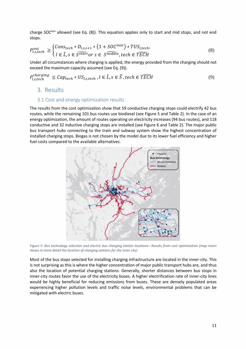
The results from the cost optimization show that 59 conductive charging stops could electrify 42 bus routes, while the remaining 101 bus routes use biodiesel (see Figure 5 and Table 2). In the case of an energy optimization, the amount of routes operating on electricity increases (94 bus routes), and 118 conductive and 32 inductive charging stops are installed (see Figure 6 and Table 2). The major public bus transport hubs connecting to the train and subway system show the highest concentration of installed charging stops. Biogas is not chosen by the model due to its lower fuel efficiency and higher fuel costs compared to the available alternatives.

Figure 5: Bus technology selection and electric bus charging station locations– Results from cost optimization (map insert shows in more detail the location of charging stations for the inner city)

Most of the bus stops selected for installing charging infrastructure are located in the inner-city. This is not surprising as this is where the higher concentration of major public transport hubs are, and thus also the location of potential charging stations. Generally, shorter distances between bus stops in inner-city routes favor the use of the electricity buses. A higher electrification rate of inner-city lines would be highly beneficial for reducing emissions from buses. These are densely populated areas experiencing higher pollution levels and traffic noise levels, environmental problems that can be mitigated with electric buses.

12

Figure 6: Bus technology selection and electric bus charging station locations– Results from energy optimization (map insert shows in more detail the location of charging stations for the inner city)

The results of the cost and energy optimization for the main parameters of the model are shown in Table 2. We also compared these results to the indicative 100% biodiesel BAU, as explained in Section 2. It should be noted that the costs estimated from the model are within an expected range when comparing to the annual bus public transport costs in Stockholm, that can be found, for example, in SLL (2013).

Table 2: Model results for cost and energy optimization compared to an indicative 100% biodiesel BAU scenario (difference in % between optimization scenarios and BAU shown in parentheses)

Biodiesel only Cost optimization Energy optimization

General

Total costs (billion SEK/year) 3.85 3.75 (-3%) 3.83 (-1%)

Total energy use (GWh/year) 648 473 (-27%) 428 (-34%)

Total emissions (MtCO2/year) 1.83 1.09 (-40%) 0.90 (-51%)

Cost breakdown

Infrastructure (million SEK/year) 0 17 (N/A) 47 (176%)

Vehicle (million SEK/year) 361 446 (+24%) 551 (+53%)

O&M (million SEK/year) 2,576 2,663 (+3%) 2,686 (+4%)

Fuel (million SEK/year) 921 630 (-32%) 555 (-40%)

Charging stations

Conductive 0 59 118

Inductive 0 0 32

Bus route technology

Biodiesel 143 101 49

Biogas 0 0 0

13

Electric (with conductive charging) 0 42 77

Electric (with inductive charging) 0 0 17

The scenarios including electrification (either applying cost or energy optimization) show costs that are within comparable range to the BAU scenario or even lower. This indicates that, if appropriately optimized, a bus network where electricity is combined with currently used liquid fuels would not result in annual costs higher than the BAU case. An issue to be considered in this context would be the upfront investment costs required for introducing electric buses at large scale. However, the design of financing strategies to make this possible is outside the scope of this paper.

The cost and energy optimization scenarios show strong reduction of energy use and emissions compared to the BAU scenario. More specifically, energy use reduction is at the range of about 30% (27% for costs optimization and 34% for energy optimization), while emission reduction ranges from 40% (cost optimization) to 51% (energy optimization).

When the costs are divided into separate groups (infrastructure and vehicle investments, operation and maintenance (O&M), and fuel costs), we observe an increase in infrastructure and vehicle investment costs. Such an increase is expected due to the costs for the charging stations (see Table 1) and the vehicles, which are higher in the case of electric buses. As more routes are selected to be electrified, more charging stations are installed, and the costs rise. However, as shown in Table 2, these costs are balanced by the decrease in fuel costs, since electricity is cheaper than biodiesel and electric engines are more energy efficient than internal combustion engines (see Table 1). This balance should be highlighted, as it illustrates that electrification of bus fleets (and possibly vehicle electrification in general) is feasible from a cost perspective due to the trade-offs achieved between infrastructure and fuel costs.

Finally, it should be noted that the highest share of costs for the scenarios shown in Table 2 is held by the O&M costs (about 65% of the total costs). This is in line with previous studies for bus transport in Sweden (SKL, 2014b; WSP, 2014a, 2014b; Xylia and Silveira, 2017), which indicate the high impact of O&M costs on public transport costs. Differences between the O&M costs in the BAU and the total system cost and energy consumption optimization scenarios can be attributed to the higher maintenance costs assumed for electric buses compared to the biodiesel buses (see Table 1). Since in the optimization scenarios the fleet comprises both biodiesel and electric buses, the O&M costs increase.

The previous indicate that the cost and energy optimization scenarios produce different results when it comes to the amount of routes that will be electrified and the number of charging locations selected. Decision makers can interpret the results and identify the optimization scenario that fits best with their priorities for bus transportation under specific local prerequisites. Each simulation requires around 60 seconds of computation time on a 64-bit operating system, with an Intel ® Core™ i7-6700 CPU @3.40Hz quad core processor and 16 GB RAM. The short computation time increases the model’s potential for use as a decision tool.

3.2 Sensitivity analysis

Cost optimization

Figure 7 illustrates the sensitivity analysis when it comes to the number of bus routes that are selected to be electrified when changing various parameters. Here, the sensitivity analysis is performed for the cost optimization, and the main focus is on the parameters that are cost-related. It can be observed that the largest impact on the electrification potential occurs from variations in the cost of biodiesel. If the biodiesel price is lower than electricity, the high infrastructure costs related to electrification become more prominent. However, higher biodiesel prices should be expected in the future, as the tax exemptions offered will be removed after 2020 (Regeringskansliet, 2015). In the case of a higher

14

biodiesel price, the number of bus routes that are selected to be electrified in the model increases significantly compared to the reference parameters assumed in Section 3.1.

Figure 7: Sensitivity analysis for the number of routes that are selected to be electrified under changing parameters in the cost optimization case

Figure 8 shows the sensitivity of the total annual costs of the system under various parameters. Here, the parameter that has by far the highest impact is the O&M costs, in line with the discussion earlier in Section 3.1.

Figure 8: Sensitivity analysis for the total annual costs under changing parameters in the cost optimization case

In the reference scenario presented in Section 3.1 the electricity price is set at 1.4 SEK/km, so the range of the sensitivity analysis is from 1 SEK/km up to 6 SEK/km. For prices above 4 SEK/km, the model only selects biodiesel as an option (see Figure 9). This can be explained by the balance of infrastructure investments and fuel costs. For higher electricity prices, the benefit of lower total fuel costs is reduced. Therefore, electric buses will most likely be selected in the case of system cost optimization, when electricity prices are sufficiently low. This also has implications for the source of electricity that is used, as electricity from renewable sources includes lower or (no) additional fuel tax. It is assumed for this model application that the electricity used is 100% certified renewable electricity. This is a realistic proposition for the case of Sweden.

0

10

20

30

40

50

60

40% 60% 80% 100% 120% 140% 160%

No

. of

ele

ctri

fie

d r

ou

tes

Parameter Change (%)

Cost Biodiesel

Charger Capacity

Cost Biogas

Cost Infrastructure

Bus Consumption

Cost Electricity

Cost O&M

2

2,5

3

3,5

4

4,5

5

5,5

40% 60% 80% 100% 120% 140% 160%

Tota

l an

nu

al c

ost

s (b

illio

n S

EK)

Parameter Change (%)

Cost O&M

Cost Biodiesel

Charger Capacity

Bus Consumption

Cost Biogas

Cost Electricity

Cost Infrastructure

15

Figure 9: Number of bus routes electrified for varying electricity prices (SEK/km)

In line with the previous, and using an average energy consumption of 1.50 kWh/km, the reference electricity price of 1.40 SEK/km, which is assumed in Section 2, translates to 0.93 SEK/kWh. This price is slightly higher than what has been assumed in previous studies on Swedish bus fleets (0.7 SEK/kWh by WSP 2014; and 0.85 SEK/kWh by Lindgren 2015). Therefore, the sensitivity analysis covers a range including both lower and higher prices than what assumed as the reference case for the model, i.e. a range from 0.66 to 4 SEK/kWh (i.e. 1 to 6 SEK/km). The upper limit of this range was intentionally set as high as 300% more than the reference value so as to be able to identify the price level at which electrification is no longer cost-competitive in relation to biodiesel. At this point, electrification is no longer chosen by the model, as shown earlier in Figure 9.

Figure 10 focuses on infrastructure and fuel costs in relation to increasing capacities for the charging stations. As the available charging power for the potential charging station locations increases, the number of bus routes that are electrified increases. As a consequence, the balance between infrastructure and fuel costs changes, in line with the discussion in Section 3.1.

Figure 10: Balance of infrastructure and fuel costs (indexed values) and number of buses electrified in relation to average available energy per charge for each station (kWh)

Energy optimization

Figure 11 shows the results of the sensitivity analysis for the energy optimization case. Here, electricity prices do not affect which lines the model selects to be electrified. This can be explained by the fact that the objective function to be minimized now is the total energy consumption. In this case, the results are not sensitive to cost-associated parameters. On the other hand, the model is proportionally equal on the positive (increase) and negative (decrease) side when it comes to changes in charging station capacity and electric bus consumption respectively. In line with the above, the model selects

0

20

40

60

80

100

120

140

160

1 1,4 2 3 4 5 6

No

. o

f e

lect

rifi

ed

ro

ute

s

Electricity price (SEK/km)

No of biodiesel bus routes

No of electric bus routes

0

10

20

30

40

50

60

0%

10%

20%

30%

40%

50%

60%

70%

80%

90%

100%

15 20 25 30 35 40

No

of

ele

ctri

fie

d r

ou

tes

IND

EX (

%)

Available energy per charge (kWh)

Cost fuel

Cost infrastructure

No of electric bus routes

16

electrification as long as the energy consumption of the electric buses remains lower than the consumption of biodiesel or biogas buses.

Figure 11: Sensitivity analysis for the number of routes that are selected to be electrified under changing parameters in the energy optimization case

Figure 12 shows the results of the sensitivity analysis on total annual energy consumption for the bus network assumed. The impact of different factors is inversely proportional to the sensitivity analysis results for the number of electrified bus routes shown in Figure 11. For example, when the energy consumption of an electric bus per kilometer increases, the number of electrified bus routes decreases and, consequently, the total energy consumption increases.

Previous studies for the impact of road grade on energy consumption of buses have shown that depending on the type of driving cycle and the increase of road grade, energy consumption can increase up to 30% (Khan and Clark, 2010). Moreover, the difference in consumption between dense city traffic and suburban routes for the Swedish case has been previously found to be 14%(Xylia and Silveira, 2017). Such variations in energy consumption are covered from the range of the sensitivity analysis assumed.

Figure 12: Sensitivity analysis for the total annual energy consumption under changing parameters in the energy optimization case

60

70

80

90

100

110

120

130

40% 60% 80% 100% 120% 140% 160%

No

. of

ele

ctri

fie

d r

ou

tes

Parameter Change (%)

Charger Capacity

Cost Electricity

Bus Consumption

200

250

300

350

400

450

500

550

40% 60% 80% 100% 120% 140% 160%

Tota

l en

erg

y co

nsu

mp

tio

n

(GW

h/y

ear

)

Parameter Change (%)

Bus Consumption

Cost Electricity

Charger Capacity

17

The range of the sensitivity analysis of energy consumption is from 40% to 160% of the value assumed for the reference case, i.e. from 0.75 to 2.25 kwh/km. this range covers the majority of the values we observed in the literature review (see Appendix Table A.1). As shown in Figure 11 and Figure 12, in the range of 80-120% change of the energy consumption (1.2 to 1.8 kWh/km), there is no significant change to the number of lines that are electrified (ca. 10% change) and the total energy consumption (ca. 13%). More significant changes occur in higher margins of the sensitivity analysis, with the difference in total energy consumption between the two extreme cases reaching 66%.

The impact that a higher average energy consumption would have for the selection of routes to be electrified and the total emissions of the system is shown in more detail in Figure 13. The sensitivity values range here from 1.5 kWh/km - the same value as the one used for the reference cases in Section 3.1 – to a maximum of 4 kWh/km, which is close to the average energy consumption of a bus running on biodiesel. The model is sensitive to the assumption of energy consumption of electric buses, and the more this consumption increases, the less bus routes are electrified. More specifically in the reference case, a total of 94 bus routes is electrified, while in the highest limit of the sensitivity analysis (4 kWh/km) the number of electrified bus routes is 63 (32% decrease). The sensitivity to this value can be attributed to the fact that as the energy consumption per kilometer increases, less bus routes are technically attractive for electrification, given the distances between the electric charging station locations.

Figure 13: Total CO2 emissions (Mt CO2/ year) and number of electrified bus routes in relation to average energy consumption of electric bus (kWh/km)

Additionally, we observe the impact of putting a minimum State-of-Charge (SOC) constraint for the energy optimization case. This constraint is placed for practical reasons, as it is beneficial for the battery health to not fall within a low SOC condition, that is, there should always be some “safety buffer” in case a charge is missed. In the reference case presented in Section 3.1, the minimum SOC of the battery at any point in the route is 30%. The minimum SOC that has generally been used in previous studies is also around 30% (Kunith et al., 2016; Olsson et al., 2016). Figure 14 shows that the selection of bus routes to be electrified in the model is not very sensitive to the minimum SOC assumption. More specifically, for the lowest SOC constraint (15%), 97 bus routes are electrified, while for the highest SOC (40%), 92 routes are electrified.

0

10

20

30

40

50

60

70

80

90

100

0

0,2

0,4

0,6

0,8

1

1,2

1,4

1,5 2 2,5 3 3,5 4

No

. o

f e

lect

rifi

ed

ro

ute

s

Emis

sio

ns

(MtC

O2

/ye

ar)

Energy consumption (kWh/km)

Total emissions

Electric bus routes

18

Figure 14: Number of bus routes electrified in relation to the minimum State-of-Charge (SOC) (%)

Finally, the impact of the assumptions for the electricity mix on the total annual CO2 emissions of the system is shown in Figure 15. Certified, emission-free electricity from renewable sources is assumed to be used. The difference in total annual emissions when a 100% renewable electricity and Swedish electricity mix are assumed reaches 163%, even though the Swedish electricity mix is one of the least emission intensive in the EU (IEA, 2015). The difference in emissions for Swedish and EU-28 electricity mix is significantly higher. The above show that, if the full environmental benefits of road transport electrification are to be harnessed, it is important to ensure that renewable electricity is chosen for charging the buses. This also implies that environmental benefits from electrification may vary depending on the local urban context and the country in question.

Figure 15: Total annual emissions (Mton CO2/year) of the bus network under different assumption for the electricity emission factor. The emission factor for renewable electricity is assumed to be 0 gCO2/kWhe. For the Swedish and the EU-28 electricity mix the emission factor is 13 and 337 gCO2/kWhe respectively (Source: IEA, 2015).

4. Conclusions

This paper focused on a key requirement for electrification of urban road transport, that is, the location of charging infrastructure for fueling a city bus network. The model developed addressed bus transport electrification at large scale and serves as a tool for supporting decisions on optimal investments to achieve fossil-free public transport. Depending on data availability, the model could be adapted to various city contexts. The model shows that, for a set of reference parameters for the case of Stockholm, the total costs for the operation of a partially electrified bus system in two optimization cases (cost and energy) marginally differ from the costs of a 100% biodiesel system. This indicates that lower operational costs and fuel prices for electric buses can balance the high

0

20

40

60

80

100

120

140

160

15% 20% 25% 30% 35% 40%

No

of

bu

s ro

ute

s

minimum SOC

No of biodiesel bus routes

No of electric bus routes

0

5

10

15

20

25

30

35

40

Tota

l em

issi

on

(M

ton

CO

2/y

ear

)

Renewable electricity mix Biodiesel only Swedish electricity mix EU electricity mix

19

investment costs for charging infrastructure. Nevertheless, the sensitivity analysis shows that biodiesel and electricity prices have a considerable impact on the selection of lines to be electrified. Electrification is not an attractive option under significantly high electricity prices.

The example tested here also shows that an optimized technology mix of buses running on liquid biofuels (in this case biodiesel) and electricity is a cost-competitive pathway. Compared to a 100% biodiesel BAU scenario, energy consumption decreased by 27% and emissions by 40% in a scenario of cost minimization. In a scenario with energy minimization, energy consumption decreased by 35% and emissions by 51%. These comparisons were made using annualized costs. However, introducing electric buses will require large upfront investments in charging infrastructure, and this will require the development of financing and business models to achieve scale. Nevertheless, the model results provide insights into what can be achieved in a long-term horizon as conditions for large scale electrification are improved.

Moreover, the results show that only a 10-25% of stops will require charging infrastructure, depending on the optimization preference, i.e. cost or energy consumption minimization. This highlights the importance of the initial selection of bus routes to be electrified and the most applicable locations for charging. Locating most of the bus charging stations at the major public transport hubs is beneficial as this is where they can be most used and the investment justified. Certainly, this will pose planning and logistic challenges that are still to be resolved particularly in very dense areas.

When it comes to the development of the model used for the analysis in this paper, future steps include detailed integration of bus schedules in a dynamic version of the model, as well as inclusion of a charging option at the bus depots. Depot charging was not included in this initial version due to lack of available data. Also depending on data availability, elevation, road grade and traffic conditions should be addressed in the most appropriate way in future updates of the model. Furthermore, this analysis only considered one bus type of 12 meters, while future versions should allow variation in bus types for each route.

Finally, the impact of large-scale bus electrification on the electricity grid needs to be carefully evaluated in future studies, where demand charges should be a central topic of interest. Since electrified road transport in Sweden holds a very low share of transport volume and electricity demand, and the business models are currently unclear, the pricing strategies of electricity providers are also unclear. In order to be able to estimate demand charges, an evaluation of the current policy framework is first needed, and then the grid should be added to the model as an additional spatial-temporal layer in order to extract information on when, where, and how much electricity will be used by the bus network.

Acknowledgements

Part of the research was developed in the Young Scientists Summer Program at the International Institute for Systems Analysis (IIASA). The Swedish Research Council FORMAS, the IIASA Tropical Flagship Initiative (TFI), and the EC project S2Biom (grant number: 608622) are gratefully acknowledged for the financial support. We would also like to thank the Transport Administration of the Stockholm City Council (SLL), in particular Kenneth Domeij and Maria Övergaard, for the data and insights provided. The first author’s research project is financed by the Swedish Energy Agency. Finally, we would like to thank the three anonymous reviewers for their valuable comments that helped improving this paper.

References

Aber, J., 2016. Electric Bus Analysis for New York City Transit. New York City. Baouche, F., Billot, R., Trigui, R., Faouzi, N.E. El, 2014. Efficient Allocation of Electric Vehicles Charging

20

Stations: Optimization Model and Application to a Dense Urban Network. IEEE Intell. Transp. Syst. Mag. doi:10.1109/MITS.2014.2324023

Bombardier, 2016. Primove e-bus [WWW Document]. URL http://primove.bombardier.com/fileadmin/primove/content/GENERAL/PUBLICATIONS/English/PT_PRIMOVE_Datasheet_2015_Braunschweig_EN_print_110dpi.pdf (accessed 9.18.16).

Cavadas, J., de Almeida Correia, G.H., Gouveia, J., 2015. A {MIP} model for locating slow-charging stations for electric vehicles in urban areas accounting for driver tours. Transp. Res. Part E Logist. Transp. Rev. 75, 188–201. doi:http://dx.doi.org/10.1016/j.tre.2014.11.005

ElectriCity, 2016. Cooperation for sustainable and attractive public transport. Gothenburg. Eudy, L., Prohaska, R., Kelly, K., Post, M., Eudy, L., Prohaska, R., Kelly, K., Post, M., 2016. Foothill

Transit Battery Electric Bus Demonstration Results Foothill Transit Battery Electric Bus Demonstration Results. Natl. Renew. Energy Lab. 60.

European Commission, 2016. Paris Agreement [WWW Document]. URL http://ec.europa.eu/clima/policies/international/negotiations/paris/index_en.htm (accessed 9.19.16).

Göhlich, D., Kunith, A., Ly, T., 2014. Technology assessment of an electric urban bus system for berlin. WIT Trans. Built Environ. 138, 137–149. doi:10.2495/UT140121

Hagberg, M., Roth, A., Bäckström, S., 2016. Analys av biogas till el för bussdrift och biogas som bränsle till bussdrift i stadstrafik 23. doi:Report C 171

Hanabusa, H., Horiguchi, R., 2011. A Study of the Analytical Method for the Location Planning of Charging Stations for Electric Vehicles, in: König, A., Dengel, A., Hinkelmann, K., Kise, K., Howlett, R.J., Jain, L.C. (Eds.), Knowledge-Based and Intelligent Information and Engineering Systems: 15th International Conference, KES 2011, Kaiserslautern, Germany, September 12-14, 2011, Proceedings, Part III. Springer, Berlin, pp. 596–605. doi:10.1007/978-3-642-23854-3_63

He, F., Yin, Y., Zhou, J., 2015. Deploying public charging stations for electric vehicles on urban road networks. Transp. Res. Part C Emerg. Technol. 60, 227–240. doi:10.1016/j.trc.2015.08.018

IEA, 2016. Energy Technology Perspectives 2016 - Towards Sustainable Urban Energy Systems. Intenrational Energy Agency, Paris.

IEA, 2015. CO2 Emissions from Fuel Combustion 2015, CO2 Emissions from Fuel Combustion. OECD Publishing, Paris. doi:10.1787/co2_fuel-2015-en

Khan, A.S., Clark, N., 2010. An Empirical Approach in Determining the Effect of Road Grade on Fuel Consumption from Transit Buses. SAE Int. J. Commer. Veh. 3, 2010-01–1950. doi:10.4271/2010-01-1950

Kunith, A., Mendelevitch, R., Goehlich, D., 2016. Electrification of a City Bus Network: An Optimization Model for Cost-Effective Placing of Charging Infrastructure and Battery Sizing of Fast Charging Electric Bus Systems (No. 1577). Berlin.

Lajunen, A., 2014. Energy consumption and cost-benefit analysis of hybrid and electric city buses. Transp. Res. Part C Emerg. Technol. 38, 1–15. doi:10.1016/j.trc.2013.10.008

Lajunen, A., Lipman, T., 2016. Lifecycle cost assessment and carbon dioxide emissions of diesel, natural gas, hybrid electric, fuel cell hybrid and electric transit buses. Energy 106, 329–342. doi:10.1016/j.energy.2016.03.075

Lindgren, L., 2015. Full electrification of Lund city bus traffic A simulation study. Lund University, Lund.

Mahmoud, M., Garnett, R., Ferguson, M., Kanaroglou, P., 2016. Electric buses: A review of alternative powertrains. Renew. Sustain. Energy Rev. 62, 673–684. doi:10.1016/j.rser.2016.05.019

McCarl, B., Meeraus, A., Eijk, P., Bussieck, M., Dirkse, S., Steacy, P., 2008. Expanded Gams User Guide Version 22.9.

Mu, Y., Wu, J., Jenkins, N., Jia, H., Wang, C., 2014. A Spatial–Temporal model for grid impact analysis of plug-in electric vehicles. Appl. Energy 114, 456–465. doi:10.1016/j.apenergy.2013.10.006

Nurhadi, L., Borén, S., Ny, H., 2014. A Sensitivity Analysis of Total Cost of Ownership for Electric

21

Public Bus Transport Systems in Swedish Medium Sized Cities. Transp. Res. Procedia 3, 818–827. doi:10.1016/j.trpro.2014.10.058

Oanda, 2016. Historical Exchange Rates [WWW Document]. URL https://www.oanda.com/solutions-for-business/historical-rates/main.html (accessed 8.31.16).

Olsson, O., Grauers, A., Pettersson, S., 2016. Method to analyze cost effectiveness of different electric bus systems, in: EVS29 International Battery, Hybrid and Fuel Cell Electric Vehicle Symposium. Montreal, pp. 1–12.

Regeringskansliet, 2015. Ansökan till EU-kommissionen om förlängd skattebefrielse av biodrivmedel. Regeringskansliet, 2013. Fossilfrihet på väg: Utredningen om fossilfri fordonstrafik SOU 2013:84.

Fritzes Offentliga Publikationer, Stockholm. Ribau, J., Viegas, R., Angelino, A., Moutinho, A., Silva, C., 2014. A new offline optimization approach

for designing a fuel cell hybrid bus. Transp. Res. Part C Emerg. Technol. 42, 14–27. doi:10.1016/j.trc.2014.02.012

Riemann, R., Wang, D.Z.W., Busch, F., 2015. Optimal location of wireless charging facilities for electric vehicles: Flow-capturing location model with stochastic user equilibrium. Transp. Res. Part C Emerg. Technol. 58, 1–12. doi:10.1016/j.trc.2015.06.022

Rogge, M., Wollny, S., Sauer, D.U., 2015. Fast Charging Battery Buses for the Electrification of Urban Public Transport—A Feasibility Study Focusing on Charging Infrastructure and Energy Storage Requirements 4587–4606. doi:10.3390/en8054587

Siemens, 2016. Siemens eBus Charging [WWW Document]. URL http://w3.siemens.com/topics/global/de/elektromobilitaet/PublishingImages/ladetechnik-busse/pdf/ebus-brochure-en.pdf (accessed 9.18.16).

Sinhuber, P., Rohlfs, W., Sauer, D.U., 2012. Study on power and energy demand for sizing the energy storage systems for electrified local public transport buses. 2012 IEEE Veh. Power Propuls. Conf. doi:10.1109/VPPC.2012.6422680

SKL, 2014a. Öppna jämförelser: Kollektivtrafik 2014. Sveriges Kommuner och Landsting, Stockholm. SKL, 2014b. Vad förklarar kollektiv- trafikens snabba kostnadsökning ? Sveriges Kommuner och

Landsting, Stockholm. SLL, 2015. Information om genomförd behovsanalys av övergång till eldriven busstrafik. Stockholm

Läns Landsting, Stockholm. SLL, 2013. Årsberättelse 2013. Stockholm Läns Landsting, Stockholm. SLL, 2009. Trafikplan 2020. Stockholm. Stockholms Stad, 2012. Framkomlighetsstrategi för Stockholm 2030. Storstockholms Lokaltrafik, 2015. Fakta om SL och länet 2014. Storstockholms Lokaltrafik,

Stockholm. Svensk Kollektivtrafik, 2015. Miljö- och fordonsdatabasen Frida. Swedish Energy Agency, 2014. Hållbara biodrivmedel och flytande biobränslen under 2013.

Eskilstuna. Tu, W., Li, Q., Fang, Z., Shaw, S., Zhou, B., Chang, X., 2015. Optimizing the locations of electric taxi

charging stations: A spatial–temporal demand coverage approach. Transp. Res. Part C Emerg. Technol. doi:10.1016/j.trc.2015.10.004

Tzeng, G.H., Lin, C.W., Opricovic, S., 2005. Multi-criteria analysis of alternative-fuel buses for public transportation. Energy Policy 33, 1373–1383. doi:10.1016/j.enpol.2003.12.014

Wirges, J., Linder, S., Kessler, A., 2012. Modelling the development of a regional charging infrastructure for electric vehicles in time and space. Eur. J. Transp. Infrastruct. Res. 12, 391–416. doi:10.1016/j.tre.2009.03.002

WSP, 2014a. Konsekvenser över elbussar i Stocholm- Kalkyl över elbussar i Stockholm. Stockholm. WSP, 2014b. Särkravens betydelse för busstrafikens kostnader. WSP Analys & Strategi Stockholm,

Stockholm. Xiang, Y., Liu, J., Li, R., Li, F., Gu, C., Tang, S., 2016. Economic planning of electric vehicle charging

stations considering traffic constraints and load profile templates. Appl. Energy 178, 647–659.

22

doi:10.1016/j.apenergy.2016.06.021 Xylia, M., Silveira, S., 2017. On the road to fossil-free public transport: The case of Swedish bus

fleets. Energy Policy 100, 397–412. doi:10.1016/j.enpol.2016.02.024 Zhu, Z.-H., Gao, Z.-Y., Zheng, J.-F., Du, H.-M., 2016. Charging station location problem of plug-in

electric vehicles. J. Transp. Geogr. 52, 11–22. doi:10.1016/j.jtrangeo.2016.02.002

23

Appendix

Table A.1: Review of previous literature regarding electric bus energy consumption

Source Energy consumption (in kWh/km)

Aber, 2016 1.7 – 1.981

ElectriCity, 2016 1.5

Eudy et al., 2016 1.34 2

Göhlich et al., 2014 2.3

Hagberg et al., 2016 1.3

Lajunen, 2014 1.5 – 1.8

Lindgren, 2015 1.5

Mahmoud et al., 2016 1.823

Nurhadi et al., 2014 0.9 - 1.14

Table A.2: Indices, variables and parameters used for the optimization algorithm

Indices

l bus route

s bus stop

tech bus technology (biodiesel, biogas, or electricity)

Binary Variables

USl,s,tech binary variable indicating if charging station is installed at bus stop {0,1}

TUSl,tech binary variable associating bus routes with specific technology {0,1}

Positive Variables

Ctotal total costs (in SEK/year)

Etotal total energy consumption (in kWh/year)

Pl,s,techcharging

power needed for charging at station (s) (in kWh)

Pl,s,techin power remaining when arriving at station (s) (in kWh)

Pl,s,techout power when leaving the station (s) (in kWh)

1 Converted from kWh/mile, assuming 1 mile = 1.6 km 2 Converted from kWh/mile, assuming 1 mile = 1.6 km 3 Converted from MJ/km, assuming 1MJ=0.27 kWh

24

Utotal total emissions (in gCO2eq/year)

Parameters

Cl,techO&M operation & maintenance costs (in SEK/year)

Cl,techfuel annual fuel costs (in SEK/year)

Cl,techinfrastructure annualized costs for infrastructure (in SEK/year)

Cl,techvehicle annualized costs for vehicles (in SEK/year)

Captech maximum power stored in the bus (biodiesel, biogas, or electricity-in kWh)

Constech power consumption per bus technology tech (in kWh/km)

Dl,s−1,s distance between the stop s-1 and s (in km)

EFtech emission factor per fuel for each technology tech (in gCO2eq/kWh)

L number of routes

L set of all bus routes

Ll length of the bus route (in km)

Nlvehicle number of vehicles deployed for operating each route

Ptechinitial power at start stop (initial fueling to maximum power capacity) (in kWh)

S number of bus stop

S set of all bus stops

Sstart number of start stops

Sstart subset of stops at the beginning of the routes

Send number of end stops

Send subset of stops at the end of the routes

Smiddle number of middle stops

Smiddle subset of stops in the middle of the routes

SOCmin minimum state-of-charge of battery (%)

TCl trips for the bus route (total annual number of trips)

TECH number of technologies

TECH set of all bus technologies