Postclosure Safety Assessment: Groundwater Modelling · Postclosure Safety Assessment: Groundwater...
188
Postclosure Safety Assessment: Groundwater Modelling March 2011 Prepared by: Geofirma Engineering Ltd. NWMO DGR-TR-2011-30
Transcript of Postclosure Safety Assessment: Groundwater Modelling · Postclosure Safety Assessment: Groundwater...
Postclosure Safety Assessment: Groundwater Modelling March 2011 Prepared by: Geofirma Engineering Ltd. NWMO DGR-TR-2011-30

Postclosure Safety Assessment: Groundwater Modelling March 2011 Prepared by: Geofirma Engineering Ltd. NWMO DGR-TR-2011-30

Postclosure SA: Groundwater Modelling - ii - March 2011
THIS PAGE HAS BEEN LEFT BLANK INTENTIONALLY
Postclosure SA: Groundwater Modelling - iii - March 2011
Document History
Title: Postclosure Safety Assessment: Groundwater Modelling
Report Number: NWMO DGR-TR-2011-30
Revision: R000 Date: March 2011
Geofirma Engineering Ltd. 1
Prepared by: A. West, J. Avis, N. Calder, R. Walsh
Reviewed by: J. Pickens
Approved by: R. Little
Nuclear Waste Management Organization
Reviewed by: H. Leung, P. Gierszewski
Accepted by: P. Gierszewski
1 Previously known as Intera Engineering Ltd.

Postclosure SA: Groundwater Modelling - iv - March 2011
THIS PAGE HAS BEEN LEFT BLANK INTENTIONALLY
Postclosure SA: Groundwater Modelling - v - March 2011
EXECUTIVE SUMMARY
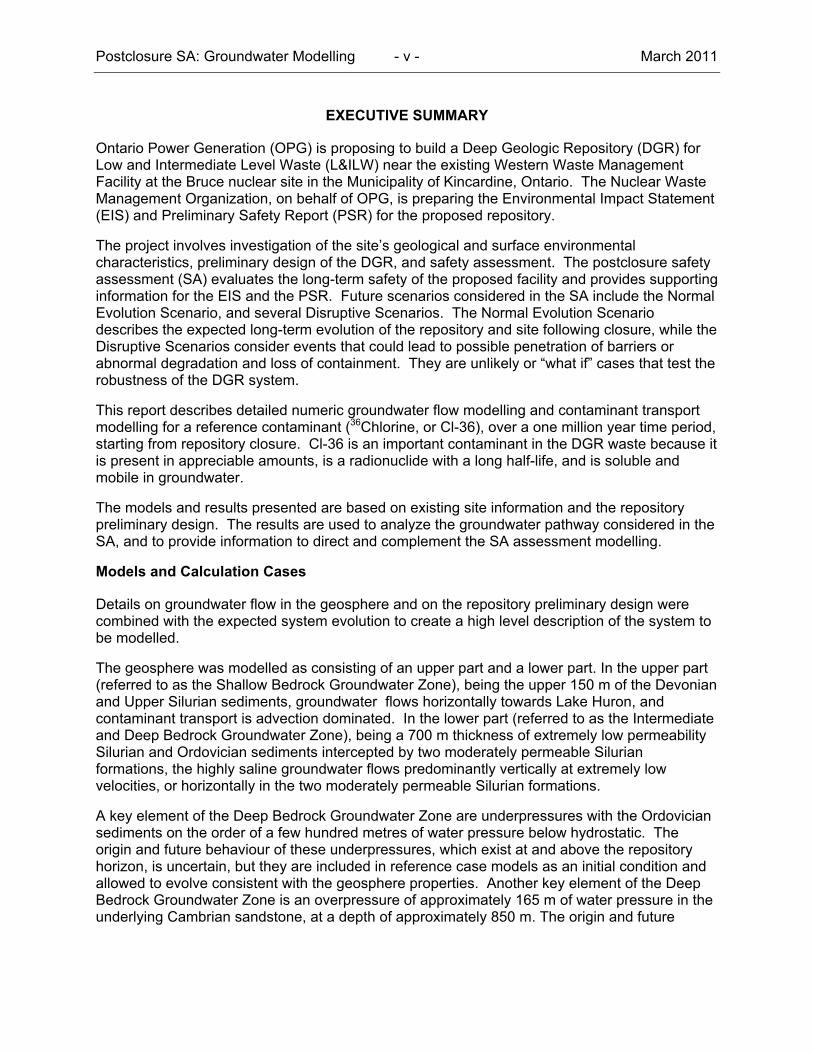
Ontario Power Generation (OPG) is proposing to build a Deep Geologic Repository (DGR) for Low and Intermediate Level Waste (L&ILW) near the existing Western Waste Management Facility at the Bruce nuclear site in the Municipality of Kincardine, Ontario. The Nuclear Waste Management Organization, on behalf of OPG, is preparing the Environmental Impact Statement (EIS) and Preliminary Safety Report (PSR) for the proposed repository.
The project involves investigation of the site’s geological and surface environmental characteristics, preliminary design of the DGR, and safety assessment. The postclosure safety assessment (SA) evaluates the long-term safety of the proposed facility and provides supporting information for the EIS and the PSR. Future scenarios considered in the SA include the Normal Evolution Scenario, and several Disruptive Scenarios. The Normal Evolution Scenario describes the expected long-term evolution of the repository and site following closure, while the Disruptive Scenarios consider events that could lead to possible penetration of barriers or abnormal degradation and loss of containment. They are unlikely or “what if” cases that test the robustness of the DGR system.
This report describes detailed numeric groundwater flow modelling and contaminant transport modelling for a reference contaminant (36Chlorine, or Cl-36), over a one million year time period, starting from repository closure. Cl-36 is an important contaminant in the DGR waste because it is present in appreciable amounts, is a radionuclide with a long half-life, and is soluble and mobile in groundwater.
The models and results presented are based on existing site information and the repository preliminary design. The results are used to analyze the groundwater pathway considered in the SA, and to provide information to direct and complement the SA assessment modelling.
Models and Calculation Cases
Details on groundwater flow in the geosphere and on the repository preliminary design were combined with the expected system evolution to create a high level description of the system to be modelled.
The geosphere was modelled as consisting of an upper part and a lower part. In the upper part (referred to as the Shallow Bedrock Groundwater Zone), being the upper 150 m of the Devonian and Upper Silurian sediments, groundwater flows horizontally towards Lake Huron, and contaminant transport is advection dominated. In the lower part (referred to as the Intermediate and Deep Bedrock Groundwater Zone), being a 700 m thickness of extremely low permeability Silurian and Ordovician sediments intercepted by two moderately permeable Silurian formations, the highly saline groundwater flows predominantly vertically at extremely low velocities, or horizontally in the two moderately permeable Silurian formations.
A key element of the Deep Bedrock Groundwater Zone are underpressures with the Ordovician sediments on the order of a few hundred metres of water pressure below hydrostatic. The origin and future behaviour of these underpressures, which exist at and above the repository horizon, is uncertain, but they are included in reference case models as an initial condition and allowed to evolve consistent with the geosphere properties. Another key element of the Deep Bedrock Groundwater Zone is an overpressure of approximately 165 m of water pressure in the underlying Cambrian sandstone, at a depth of approximately 850 m. The origin and future
Postclosure SA: Groundwater Modelling - vi - March 2011
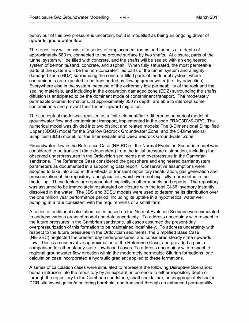
behaviour of this overpressure is uncertain, but it is modelled as being an ongoing driver of upwards groundwater flow.
The repository will consist of a series of emplacement rooms and tunnels at a depth of approximately 680 m, connected to the ground surface by two shafts. At closure, parts of the tunnel system will be filled with concrete, and the shafts will be sealed with an engineered system of bentonite/sand, concrete, and asphalt. When fully saturated, the most permeable parts of the system will be the non-concrete-filled parts of the tunnel system and a highly damaged zone (HDZ) surrounding the concrete-filled parts of the tunnel system, where contaminants are expected to be transported by flowing groundwater (i.e., by advection). Everywhere else in the system, because of the extremely low permeability of the rock and the sealing materials, and including in the excavation damaged zone (EDZ) surrounding the shafts, diffusion is anticipated to be the dominant mode of contaminant transport. The moderately permeable Silurian formations, at approximately 350 m depth, are able to intercept some contaminants and prevent their further upward migration.
The conceptual model was realized as a finite-element/finite-difference numerical model of groundwater flow and contaminant transport, implemented in the code FRAC3DVS-OPG. The numerical model was divided into two distinct and related models: The 3-Dimensional Simplified Upper (3DSU) model for the Shallow Bedrock Groundwater Zone, and the 3-Dimensional Simplified (3DS) model, for the Intermediate and Deep Bedrock Groundwater Zone.
Groundwater flow in the Reference Case (NE-RC) of the Normal Evolution Scenario model was considered to be transient (time dependent) from the initial pressure distribution, including the observed underpressures in the Ordovician sediments and overpressure in the Cambrian sandstone. The Reference Case considered the geosphere and engineered barrier system parameters as documented in a supporting data report. Conservative assumptions were adopted to take into account the effects of transient repository resaturation, gas generation and pressurization of the repository, and glaciation, which were not explicitly represented in the modelling. These factors are represented explicitly in other models and reports. The repository was assumed to be immediately resaturated on closure with the total Cl-36 inventory instantly dissolved in the water. The 3DS and 3DSU models were used to determine its distribution over the one million year performance period, including its uptake in a hypothetical water well pumping at a rate consistent with the requirements of a small farm.
A series of additional calculation cases based on the Normal Evolution Scenario were simulated to address various areas of model and data uncertainty. To address uncertainty with respect to the future pressures in the Cambrian sandstone, all cases assumed the present-day overpressurization of this formation to be maintained indefinitely. To address uncertainty with respect to the future pressures in the Ordovician sediments, the Simplified Base Case (NE-SBC) neglected the present day underpressures, and considered steady state upwards flow. This is a conservative approximation of the Reference Case, and provided a point of comparison for other steady-state flow-based cases. To address uncertainty with respect to regional groundwater flow direction within the moderately permeable Silurian formations, one calculation case incorporated a hydraulic gradient applied to these formations.
A series of calculation cases were simulated to represent the following Disruptive Scenarios: human intrusion into the repository by an exploration borehole to either repository depth or through the repository to the Cambrian sandstone; shaft seal failure; an inappropriately sealed DGR site investigation/monitoring borehole; and transport through an enhanced permeability
Postclosure SA: Groundwater Modelling - vii - March 2011
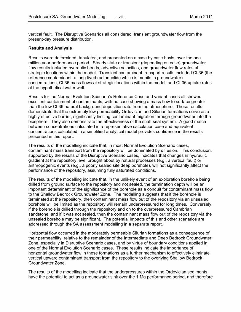
vertical fault. The Disruptive Scenarios all considered transient groundwater flow from the present-day pressure distribution.
Results and Analysis
Results were determined, tabulated, and presented on a case by case basis, over the one million year performance period. Steady state or transient (depending on case) groundwater flow results included hydraulic heads, advective velocities, and groundwater flow rates at strategic locations within the model. Transient contaminant transport results included Cl-36 (the reference contaminant, a long-lived radionuclide which is mobile in groundwater) concentrations, Cl-36 mass flows at strategic locations within the model, and Cl-36 uptake rates at the hypothetical water well.
Results for the Normal Evolution Scenario’s Reference Case and variant cases all showed excellent containment of contaminants, with no case showing a mass flow to surface greater than the low Cl-36 natural background deposition rate from the atmosphere. These results demonstrate that the extremely low permeability Ordovician and Silurian formations serve as a highly effective barrier, significantly limiting contaminant migration through groundwater into the biosphere. They also demonstrate the effectiveness of the shaft seal system. A good match between concentrations calculated in a representative calculation case and equivalent concentrations calculated in a simplified analytical model provides confidence in the results presented in this report.
The results of the modelling indicate that, in most Normal Evolution Scenario cases, contaminant mass transport from the repository will be dominated by diffusion. This conclusion, supported by the results of the Disruptive Scenario cases, indicates that changes in hydraulic gradient at the repository level brought about by natural processes (e.g., a vertical fault) or anthropogenic events (e.g., a poorly sealed site deep borehole), will not significantly affect the performance of the repository, assuming fully saturated conditions.
The results of the modelling indicate that, in the unlikely event of an exploration borehole being drilled from ground surface to the repository and not sealed, the termination depth will be an important determinant of the significance of the borehole as a conduit for contaminant mass flow to the Shallow Bedrock Groundwater Zone. The modelling suggests that if the borehole is terminated at the repository, then contaminant mass flow out of the repository via an unsealed borehole will be limited as the repository will remain underpressured for long times. Conversely, if the borehole is drilled through the repository and on to the overpressured Cambrian sandstone, and if it was not sealed, then the contaminant mass flow out of the repository via the unsealed borehole may be significant. The potential impacts of this and other scenarios are addressed through the SA assessment modelling in a separate report.
Horizontal flow occurred in the moderately permeable Silurian formations as a consequence of their permeability, relative to the remainder of the Intermediate and Deep Bedrock Groundwater Zone, especially in Disruptive Scenario cases, and by virtue of boundary conditions applied in one of the Normal Evolution Scenario cases. These results indicate the importance of horizontal groundwater flow in these formations as a further mechanism to effectively eliminate vertical upward contaminant transport from the repository to the overlying Shallow Bedrock Groundwater Zone.
The results of the modelling indicate that the underpressures within the Ordovician sediments have the potential to act as a groundwater sink over the 1 Ma performance period, and therefore

Postclosure SA: Groundwater Modelling - viii - March 2011
as a mechanism for reducing contaminant mass flow from the repository horizon to the biosphere, even when shaft seal failure is assumed.
The results of the modelling indicate that when the Ordovician underpressures were neglected (i.e., steady state vertical gradients were assumed), the contaminant mass flow to the Shallow Bedrock Groundwater Zone was higher in cases where higher hydraulic conductivities were assigned to the shaft EDZ or to the shaft seal materials. A general conclusion drawn from these results is that that the design of the shaft sealing system is important.
The results of the modelling indicate that the hypothetical water well would capture approximately 1% of the mass entering the Shallow Bedrock Groundwater Zone from the repository shaft/EDZ.
Uncertainties in the geosphere conceptual model, modelling assumptions and approaches, and model parameters were all addressed through variant calculation cases that adopted conservative assumptions or values. The two most critical uncertainties are the future pressure distribution within the Ordovician sediments and the underlying Cambrian sandstone, relating to uncertainty in the origin of the present-day pressure distribution; and the permeability of the shaft EDZ and the shaft sealing materials.
The cases analyzed in this report are complemented by gas transport modelling and assessment model results presented in companion reports. The results presented in this groundwater modelling report provide insight into the behaviour of the repository system over the 1 Ma performance period, to support the assessment of potential impacts presented in the Postclosure Safety Assessment Report.
Postclosure SA: Groundwater Modelling - ix - March 2011
TABLE OF CONTENTS
Page
EXECUTIVE SUMMARY .............................................................................................................. v
1. INTRODUCTION ............................................................................................................... 1
1.1 PURPOSE AND SCOPE ....................................................................................... 2
1.2 REPORT OUTLINE ............................................................................................... 3
2. CONCEPTUAL MODELS ................................................................................................. 4
2.1 GEOSPHERE SYSTEM OVERVIEW .................................................................... 4
2.2 REPOSITORY LOCATION AND CHARACTERISTICS ..................................... 11
2.3 NORMAL EVOLUTION AND DISRUPTIVE SCENARIOS ................................. 17
3. CALCULATION CASES ................................................................................................. 20
3.1 NORMAL EVOLUTION SCENARIO ................................................................... 23
3.2 DISRUPTIVE SCENARIOS ................................................................................. 23
4. MODEL IMPLEMENTATION .......................................................................................... 26
4.1 SOFTWARE CODES AND QUALITY ASSURANCE ......................................... 26
4.2 MODEL DOMAINS .............................................................................................. 26
4.2.1 3D Simplified Upper (3DSU) Model ................................................................ 27
4.2.2 3D Simplified (3DS) Model .............................................................................. 28
4.3 MODEL DISCRETIZATION AND PROPERTY ZONES ...................................... 29
4.3.1 3DSU Model .................................................................................................... 30
4.3.2 3DS Model ...................................................................................................... 30
4.3.2.1 Geometric Assumptions ......................................................................... 32
4.3.2.2 Discretization and Property Assignment ................................................ 33
4.3.3 3DS Model Adjustments for Calculation Cases .............................................. 38
4.3.3.1 Final Preliminary Design Cases ............................................................. 38
4.3.3.2 NE-EDZ2 Case ...................................................................................... 40
4.3.3.3 Human Intrusion and Borehole Cases ................................................... 40
4.3.3.4 Vertical Fault Cases ............................................................................... 42
Postclosure SA: Groundwater Modelling - x - March 2011
4.3.4 Discretization of Time ...................................................................................... 43
4.4 CONTAMINANT AND MATERIAL PROPERTIES.............................................. 43
4.4.1 Contaminant Properties .................................................................................. 43
4.4.2 Material Properties Used in the Reference (NE-RC Case) ............................. 43
4.4.3 Material Properties Used in Other Calculation Cases ..................................... 45
4.5 BOUNDARY AND INITIAL CONDITIONS .......................................................... 46
4.5.1 Boundary Conditions Used in the Reference (NE-RC) Case .......................... 46
4.5.2 Initial Conditions Specified in the Reference (NE-RC) Case .......................... 48
4.5.3 Boundary and Initial Conditions Used in Other Calculation Cases ................. 48
4.6 AUDIT OF FEATURES, EVENTS AND PROCESSES ....................................... 48
5. RESULTS FOR THE NORMAL EVOLUTION SCENARIO ............................................ 49
5.1 RESULTS PRESENTATION ............................................................................... 49
5.1.1 Flow Results .................................................................................................... 49
5.1.2 Transport Results ............................................................................................ 51
5.2 NE-RC: REFERENCE CASE .............................................................................. 53
5.2.1 Flow Results .................................................................................................... 54
5.2.1.1 3DS Model ............................................................................................. 54
5.2.1.2 3DSU Model........................................................................................... 56
5.2.2 Transport Results ............................................................................................ 58
5.2.2.1 3DS Model ............................................................................................. 58
5.2.2.2 3DSU Model........................................................................................... 60
5.3 NE-SBC: SIMPLIFIED BASE CASE ................................................................... 63
5.3.1 Flow Results .................................................................................................... 63
5.3.2 Transport Results ............................................................................................ 69
5.3.3 Insight Calculations ......................................................................................... 72
5.4 NE-HG: HORIZONTAL GRADIENT IN PERMEABLE SILURIAN UNITS .......... 72
5.4.1 Flow Results .................................................................................................... 72
5.4.2 Transport Results ............................................................................................ 75

Postclosure SA: Groundwater Modelling - xi - March 2011
5.5 NE-AN1: ANISOTROPY OF BEDROCK HYDRAULIC CONDUCTIVITY .......... 75
5.5.1 Flow Results .................................................................................................... 75
5.5.2 Transport Results ............................................................................................ 77
5.6 NE-AN2: ANISOTROPY OF BEDROCK EFFECTIVE DIFFUSION COEFFICIENTS .................................................................................................. 78
5.6.1 Transport Results ............................................................................................ 78
5.7 NE-EDZ1: INCREASED HYDRAULIC CONDUCTIVITY IN EDZ ....................... 80
5.7.1 Flow Results .................................................................................................... 80
5.7.2 Transport Results ............................................................................................ 82
5.8 NE-EDZ2: INCREASED HYDRAULIC CONDUCTIVITY IN EDZ WITH KEYED-IN MONOLITH ....................................................................................... 84
5.8.1 Flow Results .................................................................................................... 84
5.8.2 Transport Results ............................................................................................ 85
5.9 NE-GT5: INCREASED SHAFT SEAL HYDRAULIC CONDUCTIVITY ............... 85
5.9.1 Flow Results .................................................................................................... 85
5.9.2 Transport Results ............................................................................................ 86
5.9.2.1 3DS Model ............................................................................................. 86
5.9.2.2 3DSU Model........................................................................................... 87
5.10 NE-SE: SALINE FLUID DENSITY EFFECTS ..................................................... 89
5.10.1 Flow Results .................................................................................................... 89
5.10.2 Transport Results ............................................................................................ 90
5.11 NE-PD-RC: REFERENCE CASE, FINAL PRELIMINARY DESIGN ................... 90
5.11.1 Flow Results .................................................................................................... 90
5.11.2 Transport Results ............................................................................................ 92
5.12 NE-PD-GT5: INCREASED SHAFT HYDRAULIC CONDUCTIVITY, FINAL PRELIMINARY DESIGN ..................................................................................... 93
5.12.1 Flow Results .................................................................................................... 93
5.12.2 Transport Results ............................................................................................ 94
6. RESULTS FOR THE DISRUPTIVE SCENARIOS .......................................................... 96
6.1 HI-GR1: EXPLORATION BOREHOLE INTERSECTING THE REPOSITORY ... 96
Postclosure SA: Groundwater Modelling - xii - March 2011
6.1.1 Flow Results .................................................................................................... 96
6.1.2 Transport Results ............................................................................................ 98
6.2 HI-GR2: EXPLORATION BOREHOLE INTERSECTING THE REPOSITORY AND THE CAMBRIAN ...................................................................................... 100
6.2.1 Flow Results .................................................................................................. 100
6.2.2 Transport Results .......................................................................................... 102
6.3 SF-BC: SHAFT FAILURE BASE CASE ........................................................... 105
6.3.1 Flow Results .................................................................................................. 105
6.3.2 Transport Results .......................................................................................... 105
6.4 SF-ED: SHAFT FAILURE EXTRA DEGRADATION ........................................ 107
6.5 BH-BC: POORLY SEALED BOREHOLE ......................................................... 107
6.5.1 Flow Results .................................................................................................. 107
6.5.2 Transport Results .......................................................................................... 109
6.6 VF-BC: VERTICAL FAULT BASE CASE ......................................................... 110
6.6.1 Flow Results .................................................................................................. 110
6.6.2 Transport Results .......................................................................................... 112
6.7 VF-AL: VERTICAL FAULT ALTERNATE LOCATION ..................................... 113
6.7.1 Flow Results .................................................................................................. 113
6.7.2 Transport Results .......................................................................................... 114
7. CALCULATION CASE COMPARISONS ..................................................................... 116
8. UNCERTAINTIES ......................................................................................................... 120
8.1 CONCEPTUAL MODEL UNCERTAINTY ......................................................... 120
8.1.1 Future Pressures in Ordovician Sediments and Cambrian Sandstone ......... 120
8.1.2 Future Glaciation Events ............................................................................... 121
8.1.3 Future Horizontal Gradient in the Guelph and Salina A1 Upper Carbonate . 121
8.2 NUMERICAL MODELLING ASSUMPTIONS AND APPROACH ..................... 121
8.3 PARAMETER UNCERTAINTY ......................................................................... 122
8.3.1 Shaft EDZ and Shaft Sealing Materials Hydraulic Conductivity .................... 122
8.3.2 Geosphere Hydraulic Conductivity and Effective Diffusion Coefficient ......... 122
Postclosure SA: Groundwater Modelling - xiii - March 2011
8.4 REPOSITORY LAYOUT ................................................................................... 123
9. SUMMARY AND CONCLUSIONS ............................................................................... 124
10. REFERENCES .............................................................................................................. 126
11. ABBREVIATIONS AND ACRONYMS .......................................................................... 128
APPENDIX A: JUSTIFICATION FOR THE USE OF ENVIRONMENTAL HEADS FOR CALCULATION OF BOUNDARY AND INITIAL CONDITIONS FOR GROUNDWATER MODELLING
APPENDIX B: FRAC3DVS-OPG
APPENDIX C: METHOD USED TO SPECIFY EFFECTIVE DIFFUSION COEFFICIENTS IN FRAC3DVS-OPG
APPENDIX D: FEP AUDIT OF FRAC3DVS-OPG MODELS FOR THE POSTCLOSURE SAFETY ASSESSMENT
APPENDIX E: INSIGHT CALCULATIONS
Postclosure SA: Groundwater Modelling - xiv - March 2011
LIST OF TABLES
Page
Table 2.1: Formations ............................................................................................................... 6 Table 2.2: Relevant Hydrogeological and Transport Properties for Model Units ...................... 7 Table 2.3: Measured Horizontal Hydraulic Gradients ............................................................. 11 Table 2.4: Key System Elevations .......................................................................................... 13 Table 2.5: Hydrogeological and Transport Properties for Shaft Seal Materials ...................... 13 Table 3.1: Groundwater Modelling Cases for the Normal Evolution Scenario ........................ 24 Table 3.2: Groundwater Modelling Cases for the Disruptive Scenarios .................................. 25 Table 4.1: Radii and Cross-Sectional Areas of Combined Shaft ............................................ 30 Table 4.2: Hydrogeological and Transport Properties for Disturbed Rock and Underground
Excavations ............................................................................................................ 44
LIST OF FIGURES
Page
Figure 1.1: The DGR Concept at the Bruce Nuclear Site ........................................................... 1 Figure 1.2: Document Structure for the Postclosure Safety Assessment .................................. 2 Figure 2.1: Geological Stratigraphy at the DGR Site .................................................................. 5 Figure 2.2: Hydraulic Conductivity .............................................................................................. 8 Figure 2.3: Groundwater Density (Salinity) Profiles from the DGR-4 Site Investigation
Borehole ................................................................................................................... 9 Figure 2.4: Environmental Head Profile from DGR Site Investigation Boreholes Based on
March 2010 Monitoring Data .................................................................................. 10 Figure 2.5: Repository Layout in UTM Coordinate System; (a) Final Preliminary Design,
(b) Original Preliminary Design .............................................................................. 12 Figure 2.6: Lithology and Shaft Sealing System ...................................................................... 14 Figure 2.7: Formation Specific Distribution of Representative and Maximum EDZ Extent
Along Shaft, Including 0.5 m HDZ .......................................................................... 16 Figure 2.8: Location of the Various Features Considered in the Disruptive Scenarios Relative
to the Site Characterization Area ........................................................................... 19 Figure 3.1: Summary of Calculation Cases Considered .......................................................... 22 Figure 4.1: 3DS and 3DSU Model Domains ............................................................................. 27 Figure 4.2: Geologic Layering in the 3DS and 3DSU Groundwater Models ............................ 28 Figure 4.3: Location of the Combined Shaft (Original Preliminary Design) .............................. 29 Figure 4.4: Plan and Section of 3DSU Mesh ............................................................................ 31 Figure 4.5: Plan Outline of 3DS Repository Panel ................................................................... 32 Figure 4.6: 3DS Model Plan View of Discretization of Entire Model Domain ........................... 34 Figure 4.7: 3DS Model Plan View – Repository Detail ............................................................. 34 Figure 4.8: 3DS Model Plan View – Shaft Services Area Tunnel Detail .................................. 35 Figure 4.9: 3DS Model Plan View – Shaft, EDZ and Tunnel Detail .......................................... 35 Figure 4.10: 3DS Model Vertical Property Assignment, Full scale ............................................. 36 Figure 4.11: 3DS Model Vertical Property Assignment, Showing Monolith, HDZ, Access
Tunnels and Repository ......................................................................................... 37
Postclosure SA: Groundwater Modelling - xv - March 2011
Figure 4.12: 3DS Model Vertical Property Assignment, Showing Shaft Seals, Inner and Outer
EDZ, and HDZ below Repository (Horizontal Exaggeration 10:1) ......................... 37 Figure 4.13: 3DS Model 3D Layout of Repository, Access Tunnels, Monolith, HDZ, EDZ
(Transparent), and Shaft Sealing System .............................................................. 38 Figure 4.14: Location of the Combined Shaft (Final Preliminary Design) .................................. 39 Figure 4.15: 3DS Model 3D Layout of Repository, Access Tunnels, Monolith, HDZ, EDZ
(Transparent), and Shaft Sealing System for PD Cases ........................................ 39 Figure 4.16: Detail Showing Concrete Keyed into HDZ and EDZ in NE-EDZ2 Case ................ 40 Figure 4.17: 3DS HI-GR Model Plan View – Borehole Detail ..................................................... 41 Figure 4.18: 3DS BH-BC Model Plan View ................................................................................ 41 Figure 4.19: 3DS VF-BC Model Plan View – Fault Detail .......................................................... 42 Figure 4.20: 3DS VF-AL Model Plan View – Fault Detail ........................................................... 42 Figure 4.21: 3D View of Reference Case 3DSU Model with Boundary Conditions .................... 47 Figure 5.1: Location of Zones for Tabulation of Horizontal Groundwater Flows ...................... 50 Figure 5.2: Location of Zones for Tabulation of Vertical Groundwater Flows .......................... 51 Figure 5.3: Hydraulic Heads from Initial Condition to Steady State in Undisturbed Rock ........ 53 Figure 5.4: NE-RC Hydraulic Heads at Shaft Centreline, over 1 Ma ........................................ 54 Figure 5.5: NE-RC Model Head Contours on a Vertical Slice through Grid Y=0, at
1,000,000 Years ..................................................................................................... 55 Figure 5.6: NE-RC Hydraulic Head at Repository Elevation, at 1,000,000 Years .................... 55 Figure 5.7: NE-RC Advective Velocities at Shaft Centreline, at 1,000,000 Years .................... 56 Figure 5.8: NE-RC-3DSU Head Contours ................................................................................ 57 Figure 5.9: NE-RC-3DSU Advective Velocity Magnitude and Vectors ..................................... 57 Figure 5.10: NE-RC Cl-36 Concentration at 50,000, 100,000, 500,000, and 1,000,000 Years . 58 Figure 5.11: NE-RC Cl-36 Concentration Isovolumes at 1,000,000 Years ................................ 59 Figure 5.12: NE-RC Cl-36 Concentrations at Guelph (Left) and Repository Elevations, at
1,000,000 Years ..................................................................................................... 59 Figure 5.13: NE-RC Vertical and Horizontal Cl-36 Mass Flows ................................................. 60 Figure 5.14: Concentration Contours at 1,000,000 Years for the 3DSU Constant Source
Model ..................................................................................................................... 61 Figure 5.15: Mass Transport to Lake Huron and the Pumping Well for the 3DSU Constant
Source Model ......................................................................................................... 62 Figure 5.16: Mass Transport to Lake Huron and the Pumping Well for the 3DSU Pulse Source
Model ..................................................................................................................... 62 Figure 5.17: NE-SBC Hydraulic Head in a Vertical Slice through Grid Y=0 ............................... 63 Figure 5.18: NE-SBC Hydraulic Heads in a Vertical Slice through Shaft and Repository .......... 64 Figure 5.19: NE-SBC Hydraulic Head at Repository Elevation .................................................. 64 Figure 5.20: NE-SBC Hydraulic Heads in a Vertical Slice through the Monolith ........................ 65 Figure 5.21: NE-SBC Hydraulic Heads in a Vertical Slice through the Silurian Seals ............... 65 Figure 5.22: NE-SBC Advective Velocity Magnitude and Vectors on a Vertical Slice through
Grid Y=0 ................................................................................................................. 66 Figure 5.23: NE-SBC Advective Velocity Magnitude and Vectors in a Vertical Slice through
the Repository and Lower Shaft ............................................................................. 67 Figure 5.24: NE-SBC Advective Velocity Magnitude and Vectors at Repository Elevation ....... 67 Figure 5.25: NE-SBC Advective Velocity Magnitude and Vectors in a Vertical Slice through
the Monolith ............................................................................................................ 68 Figure 5.26: NE-SBC Advective Velocity Magnitude and Vectors in a Vertical Slice through
the Silurian Seals ................................................................................................... 68 Figure 5.27: NE-SBC Cl-36 Concentration at 50,000, 100,000, 500,000, and
1,000,000 Years ..................................................................................................... 70
Postclosure SA: Groundwater Modelling - xvi - March 2011
Figure 5.28: NE-SBC Cl-36 Concentration Isovolumes at 1,000,000 Years .............................. 70 Figure 5.29: NE-SBC Cl-36 Concentrations at Guelph (Left) and Repository Elevations, at
1,000,000 Years ..................................................................................................... 71 Figure 5.30: NE-SBC Vertical and Horizontal Cl-36 Mass Flows ............................................... 71 Figure 5.31: NE-HG Hydraulic Head in a Vertical Slice through Grid Y=0 ................................. 73 Figure 5.32: NE-HG Advective Velocity Magnitude and Vectors on a Vertical Slice
through Grid Y=0 .................................................................................................... 73 Figure 5.33: NE-HG Hydraulic Heads in a Vertical Slice through the Silurian Seals ................. 74 Figure 5.34: NE-HG Advective Velocity Magnitude and Vectors in a Vertical Slice through
the Silurian Seals ................................................................................................... 74 Figure 5.35: NE-HG Vertical and Horizontal Cl-36 Mass Flows ................................................. 75 Figure 5.36: NE-AN1 Hydraulic Head in a Vertical Slice through Grid Y=0 ............................... 76 Figure 5.37: NE-AN1 Advective Velocity Magnitude and Vectors in a Vertical Slice through
the Monolith ............................................................................................................ 76 Figure 5.38: NE-AN1 Cl-36 Concentration at 50,000, 100,000, 500,000, and
1,000,000 Years ..................................................................................................... 77 Figure 5.39: NE-AN1 Vertical and Horizontal Cl-36 Mass Flows ............................................... 78 Figure 5.40: NE-AN2 Cl-36 Concentration at 50,000, 100,000, 500,000, and
1,000,000 Years ..................................................................................................... 79 Figure 5.41: NE-AN2 Vertical and Horizontal Cl-36 Mass Flows ............................................... 79 Figure 5.42: NE-EDZ1 Hydraulic Head in a Vertical Slice through Grid Y=0 ............................. 80 Figure 5.43: NE-EDZ1 Advective Velocity Magnitude and Vectors at Repository Elevation ...... 81 Figure 5.44: NE-EDZ1 Advective Velocity Magnitude and Vectors in a Vertical Slice
through the Monolith .............................................................................................. 81 Figure 5.45: NE-EDZ1 Advective Velocities at Keyed-in Monolith, in Plan View at Elevation
of Overlying HDZ .................................................................................................... 82 Figure 5.46: NE-EDZ1 Cl-36 Concentration at 50,000, 100,000, 500,000, and
1,000,000 Years ..................................................................................................... 83 Figure 5.47: NE-EDZ1 Cl-36 Concentration Isovolumes at 1,000,000 Years ............................ 83 Figure 5.48: NE-EDZ1 Vertical and Horizontal Cl-36 Mass Flows ............................................. 84 Figure 5.49: NE-EDZ2 Advective Velocities at Keyed-in Monolith, in Plan View at Elevation
of Overlying HDZ .................................................................................................... 85 Figure 5.50: NE-GT5 Hydraulic Heads in a Vertical Slice through Shaft and Repository .......... 86 Figure 5.51: NE-GT5 Cl-36 Concentration at 50,000, 100,000, 500,000, and
1,000,000 Years ..................................................................................................... 87 Figure 5.52: NE-GT5 Vertical and Horizontal Cl-36 Mass Flows ............................................... 88 Figure 5.53: NE-GT5-3DSU Mass Flow Results ........................................................................ 88 Figure 5.54: NE-SE and NE-RC Hydraulic Heads at 0.5 a and 1 Ma, at Shaft .......................... 89 Figure 5.55: NE-SE Brine Concentrations at 0.5 a and 1 Ma, at Shaft ...................................... 89 Figure 5.56: NE-SE and NE-RC Cl-36 Concentrations at 50 ka at Repository Panel 1 ............. 90 Figure 5.57: NE-PD-RC Hydraulic Heads at Shaft Centreline, over 1 Ma ................................. 91 Figure 5.58: NE-PD-RC Hydraulic Head at Repository Elevation, at 1,000,000 Years .............. 91 Figure 5.59: NE-PD-RC Advective Velocity Magnitude and Vectors at Repository Elevation,
at 1,000,000 Years ................................................................................................. 92 Figure 5.60: NE-PD-RC Cl-36 Concentration Isovolumes at 1,000,000 Years .......................... 92 Figure 5.61: NE-PD-RC Vertical and Horizontal Cl-36 Mass Flows ........................................... 93 Figure 5.62: NE-PD-GT5 Hydraulic Heads in a Vertical Slice through Shaft and Repository .... 94 Figure 5.63: NE-PD-GT5 Cl-36 Concentration at 50,000, 100,000, 500,000, and
1,000,000 Years ..................................................................................................... 95 Figure 5.64: NE-PD-GT5 Vertical and Horizontal Cl-36 Mass Flows ......................................... 95
Postclosure SA: Groundwater Modelling - xvii - March 2011
Figure 6.1: HI-GR1 Hydraulic Heads at HI Bborehole, over 1 Ma ............................................ 96 Figure 6.2: HI-GR1 Hydraulic Heads at Shaft Centreline, over 1 Ma ....................................... 97 Figure 6.3: HI-GR1 Hydraulic Head in a Vertical Slice through Grid Y=0, at
1,000,000 Years ..................................................................................................... 97 Figure 6.4: HI-GR1 Advective Velocity Magnitude and Vectors at Repository Elevation ......... 98 Figure 6.5: HI-GR1 Cl-36 Concentration Isovolumes at 1,000,000 Years ............................... 99 Figure 6.6: HI-GR1 Vertical and Horizontal Cl-36 Mass Flows ................................................ 99 Figure 6.7: HI-GR2 Hydraulic Heads at HI Borehole, over 1 Ma ............................................ 100 Figure 6.8: HI-GR2 Hydraulic Heads at Shaft Centreline, over 1 Ma ..................................... 101 Figure 6.9: HI-GR2 Hydraulic Head in a Vertical Slice through Grid Y=0, at
1,000,000 Years ................................................................................................... 101 Figure 6.10: HI-GR2 Advective Velocity Magnitude and Vectors at Repository Elevation ....... 102 Figure 6.11: HI-GR2 Cl-36 Concentration in a Slice through the HI Borehole at 50,000,
100,000, 500,000, and 1,000,000 Years .............................................................. 103 Figure 6.12: HI-GR2 Cl-36 Concentration Isovolumes at 1,000,000 Years ............................. 103 Figure 6.13: HI-GR2 Cl-36 Concentrations at Guelph (Left) and Repository Elevations, at
1,000,000 Years ................................................................................................... 104 Figure 6.14: HI-GR2 Total Vertical and Horizontal Cl-36 Mass Flows ..................................... 104 Figure 6.15: SF-BC Hydraulic Heads at Shaft, over 1 Ma ........................................................ 105 Figure 6.16: SF-BC Advective Velocities at Shaft Centreline, at 1,000,000 Years .................. 106 Figure 6.17: SF-BC Cl-36 Concentration at 50,000, 100,000, 500,000, and 1,000,000 Years 106 Figure 6.18: BH-BC Hydraulic Heads at Exploration Borehole, over 1 Ma .............................. 107 Figure 6.19: BH-BC Hydraulic Heads at Shaft Centreline, over 1 Ma ...................................... 108 Figure 6.20: BH-BC Hydraulic Head at Repository Elevation, at 1,000,000 Years .................. 108 Figure 6.21: BH-BC Cl-36 Concentrations at Guelph (Left) and Repository Elevations, at
1,000,000 Years ................................................................................................... 109 Figure 6.22: BH-BC Vertical and Horizontal Cl-36 Mass Flows ............................................... 110 Figure 6.23: VF-BC Hydraulic Heads at the Vertical Fault, over 1 Ma ..................................... 110 Figure 6.24: VF-BC Hydraulic Heads at Shaft Centreline, over 1 Ma ...................................... 111 Figure 6.25: VF-BC Hydraulic Head in a Vertical Slice through Grid Y=0 ................................ 111 Figure 6.26: VF-BC Hydraulic Head at Repository Elevation, at 1,000,000 Years .................. 112 Figure 6.27: VF-BC Cl-36 Concentration Isovolumes at 1,000,000 Years ............................... 112 Figure 6.28: VF-BC Vertical and Horizontal Cl-36 Mass Flows ................................................ 113 Figure 6.29: VF-AL Hydraulic Head in a Vertical Slice through Grid Y=0 ................................ 114 Figure 6.30: VF-AL Cl-36 Concentration in a Shaft Centreline at 50,000, 100,000, 500,000,
and 1,000,000 Years ............................................................................................ 115 Figure 6.31: VF-AL Vertical and Horizontal Cl-36 Mass Flows ................................................ 115 Figure 7.1: Comparison of Steady State Head Profiles for Normal Evolution Scenario ......... 116 Figure 7.2: Cl-36 Vertical Mass Flow across the Salina F, and Horizontal Mass Flow in the
Silurian for all Normal Evolution Scenario Cases ................................................. 117 Figure 7.3: Cl-36 Vertical Mass Flow across the Salina F, and Horizontal Mass Flow in the
Silurian for all Disruptive Scenario Cases ............................................................ 118 Figure 7.4: Peak Cl-36 Vertical Mass Flow across the Salina F for all Cases ....................... 119

Postclosure SA: Groundwater Modelling - xviii - March 2011
THIS PAGE HAS BEEN LEFT BLANK INTENTIONALLY

Postclosure SA: Groundwater Modelling - 1 - March 2011
1. INTRODUCTION
Ontario Power Generation (OPG) is proposing to build a Deep Geologic Repository (DGR) for Low and Intermediate Level Waste (L&ILW) near the existing Western Waste Management Facility (WWMF) at the Bruce nuclear site in the Municipality of Kincardine, Ontario (Figure 1.1). The Nuclear Waste Management Organization (NWMO), on behalf of OPG, is preparing the Environmental Impact Statement (EIS) and Preliminary Safety Report (PSR) for the proposed repository.
The project involves investigation of the site’s geological and surface environmental characteristics, conceptual design of the DGR, and safety assessment. The postclosure safety assessment (SA) evaluates the long-term safety of the proposed facility and provides supporting information for the EIS (OPG 2011a) and PSR (OPG 2011b).
Figure 1.1: The DGR Concept at the Bruce Nuclear Site
Postclosure SA: Groundwater Modelling - 2 - March 2011
The work builds upon the previous safety assessment (QUINTESSA et al. 2009) and has been refined to take account of the revised waste inventory and repository design, and the greater understanding of the site that has been developed.
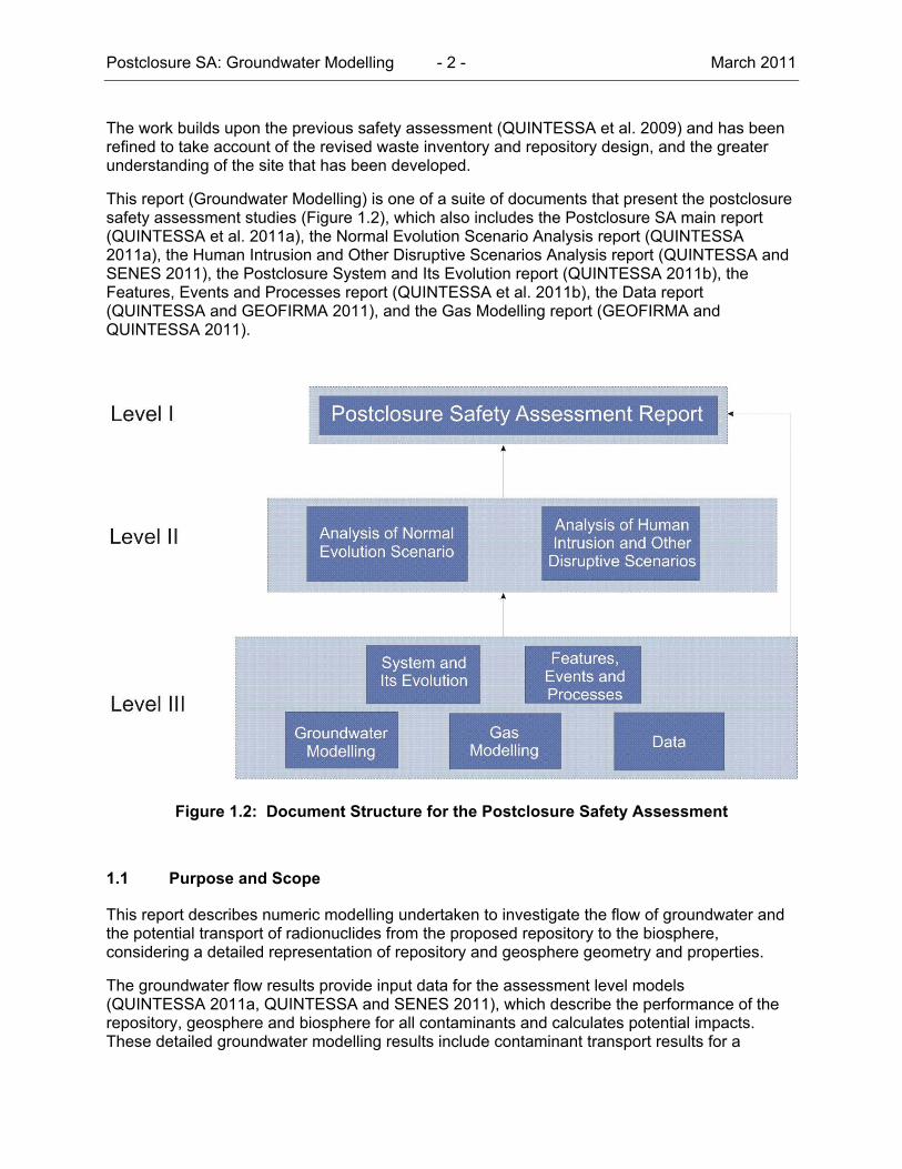
This report (Groundwater Modelling) is one of a suite of documents that present the postclosure safety assessment studies (Figure 1.2), which also includes the Postclosure SA main report (QUINTESSA et al. 2011a), the Normal Evolution Scenario Analysis report (QUINTESSA 2011a), the Human Intrusion and Other Disruptive Scenarios Analysis report (QUINTESSA and SENES 2011), the Postclosure System and Its Evolution report (QUINTESSA 2011b), the Features, Events and Processes report (QUINTESSA et al. 2011b), the Data report (QUINTESSA and GEOFIRMA 2011), and the Gas Modelling report (GEOFIRMA and QUINTESSA 2011).
Figure 1.2: Document Structure for the Postclosure Safety Assessment
1.1 Purpose and Scope
This report describes numeric modelling undertaken to investigate the flow of groundwater and the potential transport of radionuclides from the proposed repository to the biosphere, considering a detailed representation of repository and geosphere geometry and properties.
The groundwater flow results provide input data for the assessment level models (QUINTESSA 2011a, QUINTESSA and SENES 2011), which describe the performance of the repository, geosphere and biosphere for all contaminants and calculates potential impacts. These detailed groundwater modelling results include contaminant transport results for a
Postclosure SA: Groundwater Modelling - 3 - March 2011
reference contaminant 36Chlorine (Cl-36), which provides the assessment level models with a verification point. Cl-36 has been identified as a primary contaminant of concern, being present in the waste inventory in sufficient quantity, having a long half life (300 ka), and being mobile in water.
The modelling described in this report considered a variety of groundwater flow and contaminant transport scenarios over a one million year performance period, starting at repository closure. A Reference Case was developed which approximates the Normal Evolution Scenario documented in Chapter 7 of the System and Its Evolution report (QUINTESSA 2011b), while other calculation cases allow for an assessment of sensitivity of the results to various assumptions and parameters.
In addition to the Reference Case and other Normal Evolution calculation cases, a variety of cases were developed to assess the effect of possible Disruptive Scenarios (QUINTESSA and SENES 2011) on groundwater flow and contaminant transport.
1.2 Report Outline
The report is organized as follows:
Chapter 2 describes the conceptual models of groundwater flow and transport and the approach used to create numeric models representing the conceptual models;
Chapter 3 describes the defined calculation cases; Chapter 4 provides an overview of the implementation of the detailed numeric models; Chapter 5 presents results for the Normal Evolution Scenario calculation cases ; Chapter 6 presents results for the Disruptive Scenarios calculation cases; Chapter 7 provides an overall comparison and assessment of the calculation cases for the
Normal Evolution and Disruptive Scenarios; Chapter 8 describes uncertainties in modelling the scenarios and in the results, and how
these were addressed in the current study; and Chapter 9 provides overall conclusions from the detailed groundwater modelling.
The report has been written for a technical audience that is familiar with the scope and objectives of the DGR project, the Bruce nuclear site, and the process of assessing the long-term safety of a deep geologic repository.
Postclosure SA: Groundwater Modelling - 4 - March 2011
2. CONCEPTUAL MODELS
This section of the report describes the overall conceptual model of the groundwater system at the Bruce nuclear site; the basic characteristics of the proposed repository and its relationship to the geosphere; and the modelling approaches selected to simulate the integrated repository and geosphere system.
2.1 Geosphere System Overview
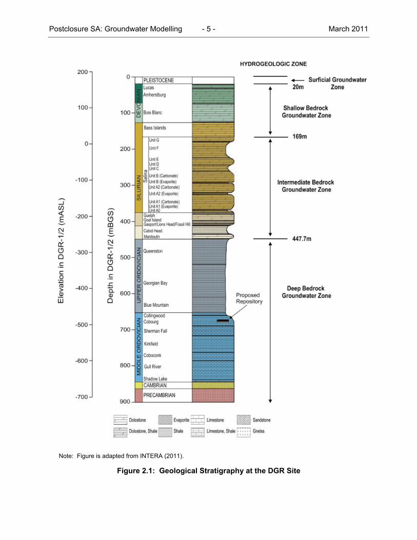
As described in Section 2.3.6.2 of the System and Its Evolution report (QUINTESSA 2011b), groundwater flow at the Bruce nuclear site can be divided into four basic zones, delineated by stratigraphy as shown in Figure 2.1. The groundwater zones are as follows.
1. Surficial deposits (overburden) groundwater zone – Local flow of fresh water providing precipitation driven recharge to the underlying Shallow Bedrock Groundwater Zone. The surficial zone is approximately 20 m thick.
2. Shallow Bedrock Groundwater Zone – The relatively high permeability sequence consisting of Devonian and Upper Silurian (Bass Island only) sediments to an approximate depth of 170 m below ground surface (mBGS). Groundwater in this zone is fresh to brackish and flow is primarily horizontal, driven by topographic features with discharge to Lake Huron. Hydraulic gradients and permeability in this zone are sufficiently high to create advection dominated transport.
3. Intermediate Bedrock Groundwater Zone – Approximately 280 m thickness of Silurian sediments from the Salina G down to the Manitoulin, at an approximate depth of 450 mBGS. These formations are primarily low-permeability shales and dolostones, with some extremely low permeability anhydrite beds. Also included are the Salina A1 Upper Carbonate and Guelph formations, which exhibit moderate permeability. Regional horizontal groundwater flow is expected to exist in the latter formations, albeit under very low horizontal gradients. Groundwater in the zone is saline to extremely saline (20 to 310 g/L).
4. Deep Bedrock Groundwater Zone - All stratigraphic units below the Manitoulin. Groundwater in this zone is extremely saline (150 to 350 g/L), and transport in the low-permeability Ordovician shale and limestone is expected to be diffusion dominated.
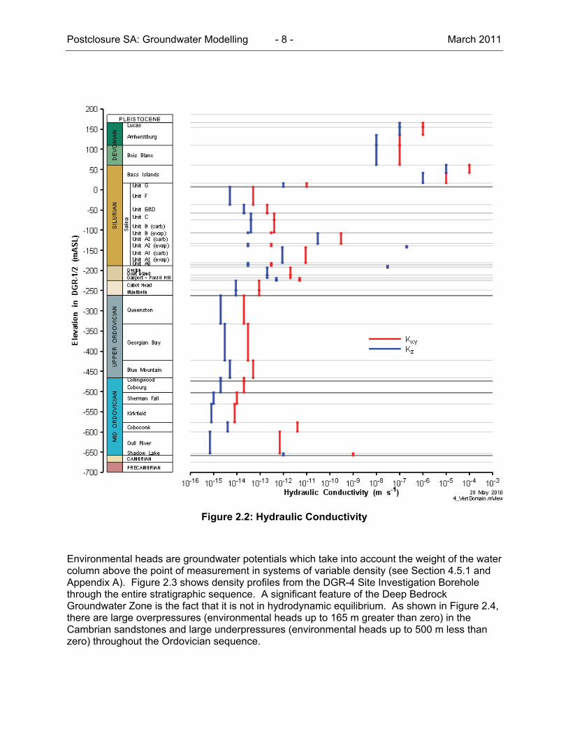
The groundwater zones are shown in Figure 2.1, while the stratigraphy is summarized in Table 2.1. The properties of the various formations that are relevant to the detailed groundwater modelling are summarized in Table 2.2, while the horizontal and vertical hydraulic conductivity values (Kxy and Kz, respectively) are shown in Figure 2.2 (Table 5.5 of the Data report, QUINTESSA and GEOFIRMA 2011).
Postclosure SA: Groundwater Modelling - 5 - March 2011
Note: Figure is adapted from INTERA (2011).
Figure 2.1: Geological Stratigraphy at the DGR Site
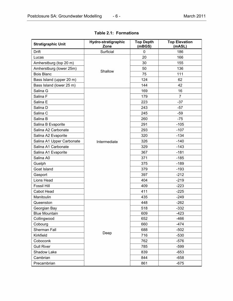
Postclosure SA: Groundwater Modelling - 6 - March 2011
Table 2.1: Formations
Stratigraphic Unit Hydro-stratigraphic
Zone Top Depth Top Elevation
(mBGS) (mASL)
Drift Surficial 0 186
Lucas
Shallow
20 166
Amherstburg (top 20 m) 30 155
Amherstburg (lower 25m) 50 136
Bois Blanc 75 111
Bass Island (upper 20 m) 124 62
Bass Island (lower 25 m) 144 42
Salina G
Intermediate
169 16
Salina F 179 7
Salina E 223 -37
Salina D 243 -57
Salina C 245 -59
Salina B 260 -75
Salina B Evaporite 291 -105
Salina A2 Carbonate 293 -107
Salina A2 Evaporite 320 -134
Salina A1 Upper Carbonate 326 -140
Salina A1 Carbonate 329 -143
Salina A1 Evaporite 367 -181
Salina A0 371 -185
Guelph 375 -189
Goat Island 379 -193
Gasport 397 -212
Lions Head 404 -219
Fossil Hill 409 -223
Cabot Head 411 -225
Manitoulin 435 -249
Queenston
Deep
448 -262
Georgian Bay 518 -332 Blue Mountain 609 -423 Collingwood 652 -466
Cobourg 660 -474
Sherman Fall 688 -502
Kirkfield 716 -530
Coboconk 762 -576
Gull River 785 -599
Shadow Lake 839 -653
Cambrian 844 -658
Precambrian 861 -675
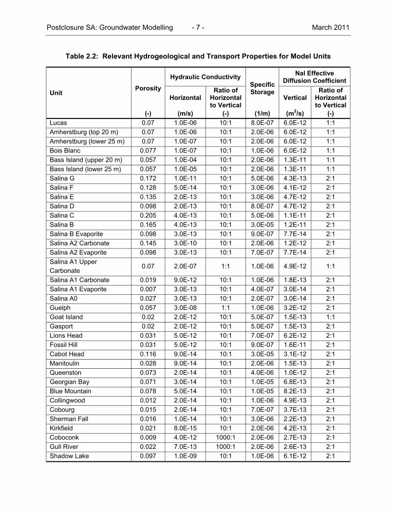
Postclosure SA: Groundwater Modelling - 7 - March 2011
Table 2.2: Relevant Hydrogeological and Transport Properties for Model Units
Unit Porosity
Hydraulic Conductivity Specific Storage
Nal Effective Diffusion Coefficient
Horizontal Ratio of
Horizontal to Vertical
Vertical Ratio of
Horizontal to Vertical
(-) (m/s) (-) (1/m) (m2/s) (-)
Lucas 0.07 1.0E-06 10:1 8.0E-07 6.0E-12 1:1
Amherstburg (top 20 m) 0.07 1.0E-06 10:1 2.0E-06 6.0E-12 1:1
Amherstburg (lower 25 m) 0.07 1.0E-07 10:1 2.0E-06 6.0E-12 1:1
Bois Blanc 0.077 1.0E-07 10:1 1.0E-06 6.0E-12 1:1
Bass Island (upper 20 m) 0.057 1.0E-04 10:1 2.0E-06 1.3E-11 1:1
Bass Island (lower 25 m) 0.057 1.0E-05 10:1 2.0E-06 1.3E-11 1:1
Salina G 0.172 1.0E-11 10:1 5.0E-06 4.3E-13 2:1
Salina F 0.128 5.0E-14 10:1 3.0E-06 4.1E-12 2:1
Salina E 0.135 2.0E-13 10:1 3.0E-06 4.7E-12 2:1
Salina D 0.098 2.0E-13 10:1 8.0E-07 4.7E-12 2:1
Salina C 0.205 4.0E-13 10:1 5.0E-06 1.1E-11 2:1
Salina B 0.165 4.0E-13 10:1 3.0E-05 1.2E-11 2:1
Salina B Evaporite 0.098 3.0E-13 10:1 9.0E-07 7.7E-14 2:1
Salina A2 Carbonate 0.145 3.0E-10 10:1 2.0E-06 1.2E-12 2:1
Salina A2 Evaporite 0.098 3.0E-13 10:1 7.0E-07 7.7E-14 2:1
Salina A1 Upper Carbonate
0.07 2.0E-07 1:1 1.0E-06 4.9E-12 1:1
Salina A1 Carbonate 0.019 9.0E-12 10:1 1.0E-06 1.8E-13 2:1
Salina A1 Evaporite 0.007 3.0E-13 10:1 4.0E-07 3.0E-14 2:1
Salina A0 0.027 3.0E-13 10:1 2.0E-07 3.0E-14 2:1
Guelph 0.057 3.0E-08 1:1 1.0E-06 3.2E-12 2:1
Goat Island 0.02 2.0E-12 10:1 5.0E-07 1.5E-13 1:1
Gasport 0.02 2.0E-12 10:1 5.0E-07 1.5E-13 2:1
Lions Head 0.031 5.0E-12 10:1 7.0E-07 6.2E-12 2:1
Fossil Hill 0.031 5.0E-12 10:1 9.0E-07 1.6E-11 2:1
Cabot Head 0.116 9.0E-14 10:1 3.0E-05 3.1E-12 2:1
Manitoulin 0.028 9.0E-14 10:1 2.0E-06 1.5E-13 2:1
Queenston 0.073 2.0E-14 10:1 4.0E-06 1.0E-12 2:1
Georgian Bay 0.071 3.0E-14 10:1 1.0E-05 6.8E-13 2:1
Blue Mountain 0.078 5.0E-14 10:1 1.0E-05 8.2E-13 2:1
Collingwood 0.012 2.0E-14 10:1 1.0E-06 4.9E-13 2:1
Cobourg 0.015 2.0E-14 10:1 7.0E-07 3.7E-13 2:1
Sherman Fall 0.016 1.0E-14 10:1 3.0E-06 2.2E-13 2:1
Kirkfield 0.021 8.0E-15 10:1 2.0E-06 4.2E-13 2:1
Coboconk 0.009 4.0E-12 1000:1 2.0E-06 2.7E-13 2:1
Gull River 0.022 7.0E-13 1000:1 2.0E-06 2.6E-13 2:1
Shadow Lake 0.097 1.0E-09 10:1 1.0E-06 6.1E-12 2:1
Postclosure SA: Groundwater Modelling - 8 - March 2011
Figure 2.2: Hydraulic Conductivity
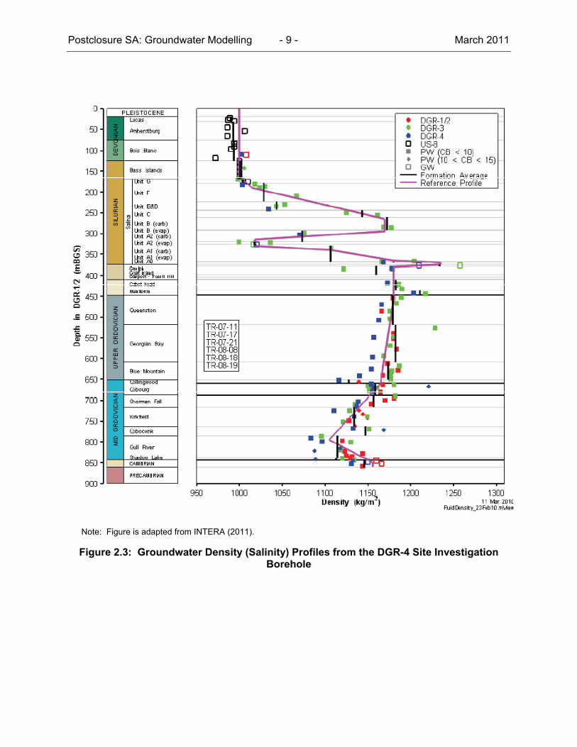
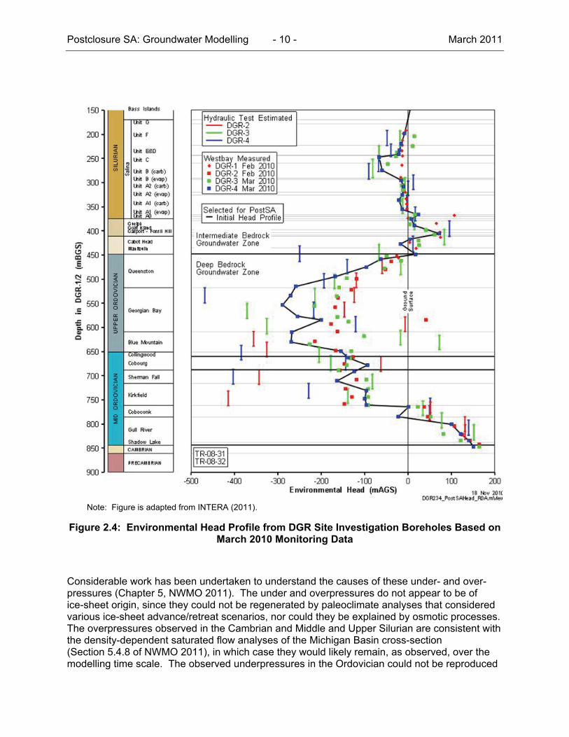
Environmental heads are groundwater potentials which take into account the weight of the water column above the point of measurement in systems of variable density (see Section 4.5.1 and Appendix A). Figure 2.3 shows density profiles from the DGR-4 Site Investigation Borehole through the entire stratigraphic sequence. A significant feature of the Deep Bedrock Groundwater Zone is the fact that it is not in hydrodynamic equilibrium. As shown in Figure 2.4, there are large overpressures (environmental heads up to 165 m greater than zero) in the Cambrian sandstones and large underpressures (environmental heads up to 500 m less than zero) throughout the Ordovician sequence.
Postclosure SA: Groundwater Modelling - 9 - March 2011
Note: Figure is adapted from INTERA (2011).
Figure 2.3: Groundwater Density (Salinity) Profiles from the DGR-4 Site Investigation Borehole
Postclosure SA: Groundwater Modelling - 10 - March 2011
Note: Figure is adapted from INTERA (2011).
Figure 2.4: Environmental Head Profile from DGR Site Investigation Boreholes Based on March 2010 Monitoring Data
Considerable work has been undertaken to understand the causes of these under- and over- pressures (Chapter 5, NWMO 2011). The under and overpressures do not appear to be of ice-sheet origin, since they could not be regenerated by paleoclimate analyses that considered various ice-sheet advance/retreat scenarios, nor could they be explained by osmotic processes. The overpressures observed in the Cambrian and Middle and Upper Silurian are consistent with the density-dependent saturated flow analyses of the Michigan Basin cross-section (Section 5.4.8 of NWMO 2011), in which case they would likely remain, as observed, over the modelling time scale. The observed underpressures in the Ordovician could not be reproduced
Postclosure SA: Groundwater Modelling - 11 - March 2011
using the density-dependent saturated flow analyses but could be reproduced by assuming the presence of a non-wetting immiscible gas phase in the rock, in which case they would likely evolve with time (Section 5.4.9 of NWMO 2011).
The fact that the observed underpressures and overpressures are large indicates that the permeability is very low and there is no connectivity or transmissivity to a fracture network at or near the DGR site.
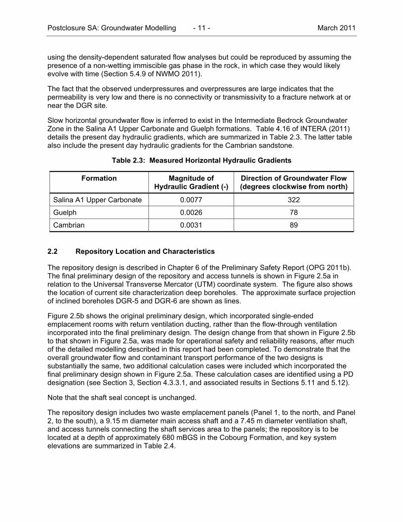
Slow horizontal groundwater flow is inferred to exist in the Intermediate Bedrock Groundwater Zone in the Salina A1 Upper Carbonate and Guelph formations. Table 4.16 of INTERA (2011) details the present day hydraulic gradients, which are summarized in Table 2.3. The latter table also include the present day hydraulic gradients for the Cambrian sandstone.
Table 2.3: Measured Horizontal Hydraulic Gradients
Formation Magnitude of Hydraulic Gradient (-)
Direction of Groundwater Flow (degrees clockwise from north)
Salina A1 Upper Carbonate 0.0077 322
Guelph 0.0026 78
Cambrian 0.0031 89
2.2 Repository Location and Characteristics
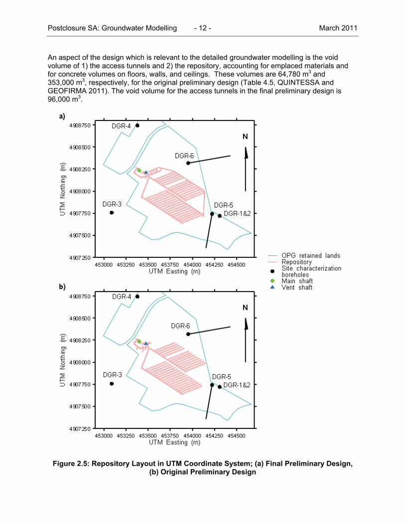
The repository design is described in Chapter 6 of the Preliminary Safety Report (OPG 2011b). The final preliminary design of the repository and access tunnels is shown in Figure 2.5a in relation to the Universal Transverse Mercator (UTM) coordinate system. The figure also shows the location of current site characterization deep boreholes. The approximate surface projection of inclined boreholes DGR-5 and DGR-6 are shown as lines.
Figure 2.5b shows the original preliminary design, which incorporated single-ended emplacement rooms with return ventilation ducting, rather than the flow-through ventilation incorporated into the final preliminary design. The design change from that shown in Figure 2.5b to that shown in Figure 2.5a, was made for operational safety and reliability reasons, after much of the detailed modelling described in this report had been completed. To demonstrate that the overall groundwater flow and contaminant transport performance of the two designs is substantially the same, two additional calculation cases were included which incorporated the final preliminary design shown in Figure 2.5a. These calculation cases are identified using a PD designation (see Section 3, Section 4.3.3.1, and associated results in Sections 5.11 and 5.12).
Note that the shaft seal concept is unchanged.
The repository design includes two waste emplacement panels (Panel 1, to the north, and Panel 2, to the south), a 9.15 m diameter main access shaft and a 7.45 m diameter ventilation shaft, and access tunnels connecting the shaft services area to the panels; the repository is to be located at a depth of approximately 680 mBGS in the Cobourg Formation, and key system elevations are summarized in Table 2.4.
Postclosure SA: Groundwater Modelling - 12 - March 2011
An aspect of the design which is relevant to the detailed groundwater modelling is the void volume of 1) the access tunnels and 2) the repository, accounting for emplaced materials and for concrete volumes on floors, walls, and ceilings. These volumes are 64,780 m3 and 353,000 m3, respectively, for the original preliminary design (Table 4.5, QUINTESSA and GEOFIRMA 2011). The void volume for the access tunnels in the final preliminary design is 96,000 m3.
Figure 2.5: Repository Layout in UTM Coordinate System; (a) Final Preliminary Design, (b) Original Preliminary Design
Postclosure SA: Groundwater Modelling - 13 - March 2011
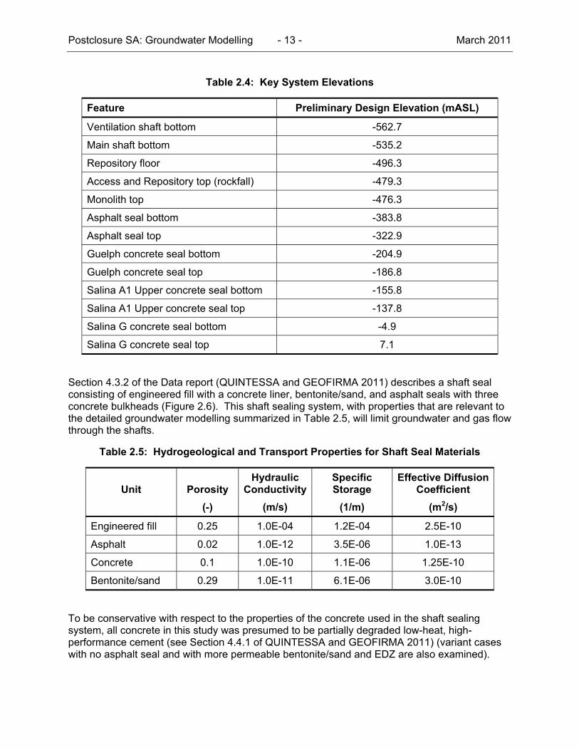
Table 2.4: Key System Elevations
Feature Preliminary Design Elevation (mASL)
Ventilation shaft bottom -562.7
Main shaft bottom -535.2
Repository floor -496.3
Access and Repository top (rockfall) -479.3
Monolith top -476.3
Asphalt seal bottom -383.8
Asphalt seal top -322.9
Guelph concrete seal bottom -204.9
Guelph concrete seal top -186.8
Salina A1 Upper concrete seal bottom -155.8
Salina A1 Upper concrete seal top -137.8
Salina G concrete seal bottom -4.9
Salina G concrete seal top 7.1
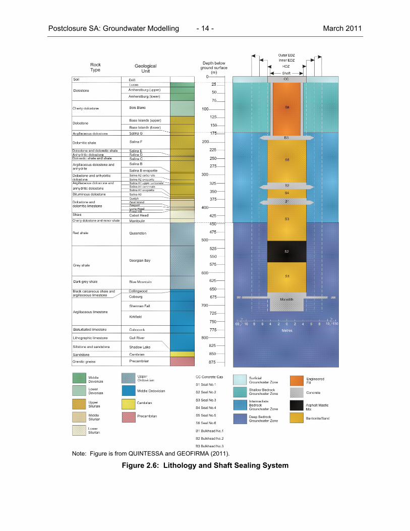
Section 4.3.2 of the Data report (QUINTESSA and GEOFIRMA 2011) describes a shaft seal consisting of engineered fill with a concrete liner, bentonite/sand, and asphalt seals with three concrete bulkheads (Figure 2.6). This shaft sealing system, with properties that are relevant to the detailed groundwater modelling summarized in Table 2.5, will limit groundwater and gas flow through the shafts.
Table 2.5: Hydrogeological and Transport Properties for Shaft Seal Materials
Unit Porosity Hydraulic
ConductivitySpecific Storage
Effective Diffusion Coefficient
(-) (m/s) (1/m) (m2/s)
Engineered fill 0.25 1.0E-04 1.2E-04 2.5E-10
Asphalt 0.02 1.0E-12 3.5E-06 1.0E-13
Concrete 0.1 1.0E-10 1.1E-06 1.25E-10
Bentonite/sand 0.29 1.0E-11 6.1E-06 3.0E-10
To be conservative with respect to the properties of the concrete used in the shaft sealing system, all concrete in this study was presumed to be partially degraded low-heat, high-performance cement (see Section 4.4.1 of QUINTESSA and GEOFIRMA 2011) (variant cases with no asphalt seal and with more permeable bentonite/sand and EDZ are also examined).
Postclosure SA: Groundwater Modelling - 14 - March 2011
Note: Figure is from QUINTESSA and GEOFIRMA (2011).
Figure 2.6: Lithology and Shaft Sealing System
Postclosure SA: Groundwater Modelling - 15 - March 2011
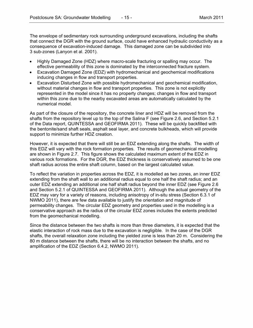
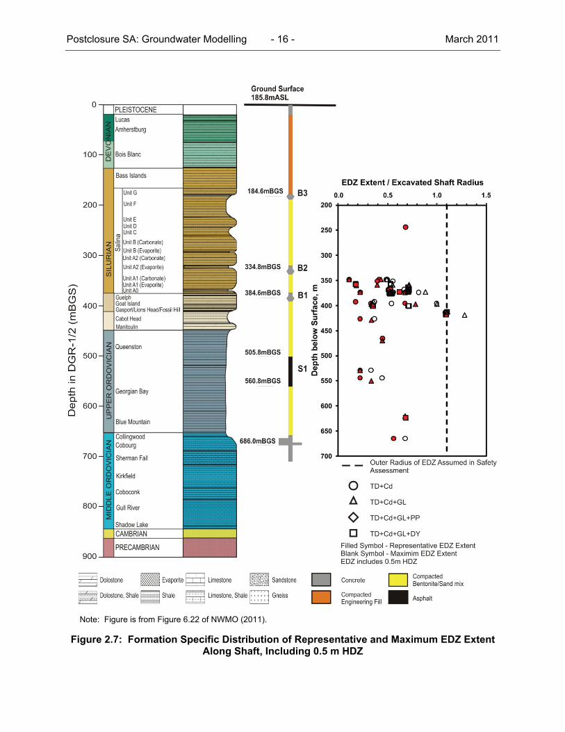
The envelope of sedimentary rock surrounding underground excavations, including the shafts that connect the DGR with the ground surface, could have enhanced hydraulic conductivity as a consequence of excavation-induced damage. This damaged zone can be subdivided into 3 sub-zones (Lanyon et al. 2001).
Highly Damaged Zone (HDZ) where macro-scale fracturing or spalling may occur. The effective permeability of this zone is dominated by the interconnected fracture system.
Excavation Damaged Zone (EDZ) with hydromechanical and geochemical modifications inducing changes in flow and transport properties.
Excavation Disturbed Zone with possible hydromechanical and geochemical modification, without material changes in flow and transport properties. This zone is not explicitly represented in the model since it has no property changes; changes in flow and transport within this zone due to the nearby excavated areas are automatically calculated by the numerical model.
As part of the closure of the repository, the concrete liner and HDZ will be removed from the shafts from the repository level up to the top of the Salina F (see Figure 2.6, and Section 5.2.1 of the Data report, QUINTESSA and GEOFIRMA 2011). These will be quickly backfilled with the bentonite/sand shaft seals, asphalt seal layer, and concrete bulkheads, which will provide support to minimize further HDZ creation.
However, it is expected that there will still be an EDZ extending along the shafts. The width of this EDZ will vary with the rock formation properties. The results of geomechanical modelling are shown in Figure 2.7. This figure shows the calculated maximum extent of the EDZ in various rock formations. For the DGR, the EDZ thickness is conservatively assumed to be one shaft radius across the entire shaft column, based on the largest calculated value.
To reflect the variation in properties across the EDZ, it is modelled as two zones, an inner EDZ extending from the shaft wall to an additional radius equal to one half the shaft radius; and an outer EDZ extending an additional one half shaft radius beyond the inner EDZ (see Figure 2.6 and Section 5.2.1 of QUINTESSA and GEOFIRMA 2011). Although the actual geometry of the EDZ may vary for a variety of reasons, including anisotropy of in-situ stress (Section 6.3.1 of NWMO 2011), there are few data available to justify the orientation and magnitude of permeability changes. The circular EDZ geometry and properties used in the modelling is a conservative approach as the radius of the circular EDZ zones includes the extents predicted from the geomechanical modelling.
Since the distance between the two shafts is more than three diameters, it is expected that the elastic interaction of rock mass due to the excavation is negligible. In the case of the DGR shafts, the overall relaxation zone including the yielded zone is less than 20 m. Considering the 80 m distance between the shafts, there will be no interaction between the shafts, and no amplification of the EDZ (Section 6.4.2, NWMO 2011).
Postclosure SA: Groundwater Modelling - 16 - March 2011
Note: Figure is from Figure 6.22 of NWMO (2011).
Figure 2.7: Formation Specific Distribution of Representative and Maximum EDZ Extent Along Shaft, Including 0.5 m HDZ
Postclosure SA: Groundwater Modelling - 17 - March 2011
2.3 Normal Evolution and Disruptive Scenarios
The Normal Evolution Scenario (Chapter 7 of the System and Its Evolution report, QUINTESSA 2011b) describes in detail the expected evolution of the geosphere, repository system including waste, and climate, as a function of time. The Normal Evolution Scenario provided the basis for the detailed numerical modelling, with the following assumptions and simplifications.
1. Climatic impacts due to glaciation were not explicitly modelled. Such impacts could include changes in mechanical and hydraulic loading of the geosphere associated with the advance and retreat of glaciers over the 1 Ma year timeframe. The omission of such effects from the detailed groundwater flow and contaminant transport modelling was justified as follows: a) it is anticipated that ice sheets will not cover the site for several tens of thousands of years, during which time there will be significant decay of most radionuclides of interest; b) regional geological data and hydrogeological modelling (Section 5.4.6 of NWMO 2011) indicate that glacial advance and retreat has had little influence on the Intermediate and Deep Bedrock Groundwater Zones over the last one million years; and c) conservative assumptions about rockfall within the facility account for the effects of mechanical loading from glacial advance and retreat (Section 4.3.2.1).
2. Repository resaturation was assumed instantaneous at closure, with no gas generated. Detailed gas (two-phase) modelling (GEOFIRMA and QUINTESSA 2011) indicated that the repository may take well in excess of a million years to fully resaturate, due in part to the low permeability of the host rock. To be conservative, this resaturation delay was ignored in the current modelling, and groundwater transport of radionuclides was assumed to commence immediately on repository closure.
3. Cambrian overpressure was retained, and Ordovician underpressure was retained or
ignored, depending on case. The present-day overpressure of the Cambrian was assumed to persist over the million year time frame. This is a conservative assumption as it ensures upwards groundwater flow from the Cambrian towards the repository. To account for the Ordovician underpressures, the environmental head profile (Figure 2.4) was used as an initial condition for all transient models, including the Reference Case (see Section 4.5.2). To be conservative, cases without the Ordovician underpressures were also used.
4. Contaminant release was assumed to be instantaneous. The rate of contaminant release
into dissolved form will depend upon repository resaturation, waste form degradation and dissolution processes. To be conservative, the entire Cl-36 (the key contaminant considered in this study, see Section 1.1) inventory was assumed to dissolve in the saturated repository volume at time zero.
5. Groundwater was generally assumed to be of constant density, but density effects were also
assessed. The salinity of groundwater at the site varies from fresh in the Shallow Bedrock Groundwater Zone to extremely saline in the Intermediate and Deep Bedrock Groundwater Zones, and density in the order of 1200 kg/m3 (see Figure 2.3) is present. Variability in groundwater density can influence groundwater flow, causing for example the downwards mobility of a source of shallow dense groundwater, and the stagnation of deep dense groundwater in an otherwise flowing system. To significantly simplify the modelling, density effects were omitted from the majority of the detailed groundwater flow and contaminant transport modelling. The omission of such effects is generally conservative and was justified

Postclosure SA: Groundwater Modelling - 18 - March 2011
as follows: a) the salinity profiles were included in the regional modelling presented in the Geosynthesis, and were found to have a small effect; b) environmental heads, which account for the actual density profile, were used for all boundary and initial specified hydraulic heads (see Appendix A); and c) salinity within the deep bedrock groundwater system is quite uniform, and density driven flow within this zone is not anticipated.
6. No partial gas saturation in the Ordovician. According to INTERA (2011) and NWMO (2011), the pore space in the Ordovician sediments is partially saturated with methane. Partial gas saturation effectively reduces the relative permeability of water, and reduces the pore space available for diffusion of dissolved phase contaminants. In the current study, fully saturated conditions were assumed, and the saturated hydraulic conductivities were conservatively assumed.
The following four Disruptive Scenarios are identified in Chapter 8 of the System and Its Evolution report (QUINTESSA 2011b), in which the major geosphere barriers could potentially be breached.
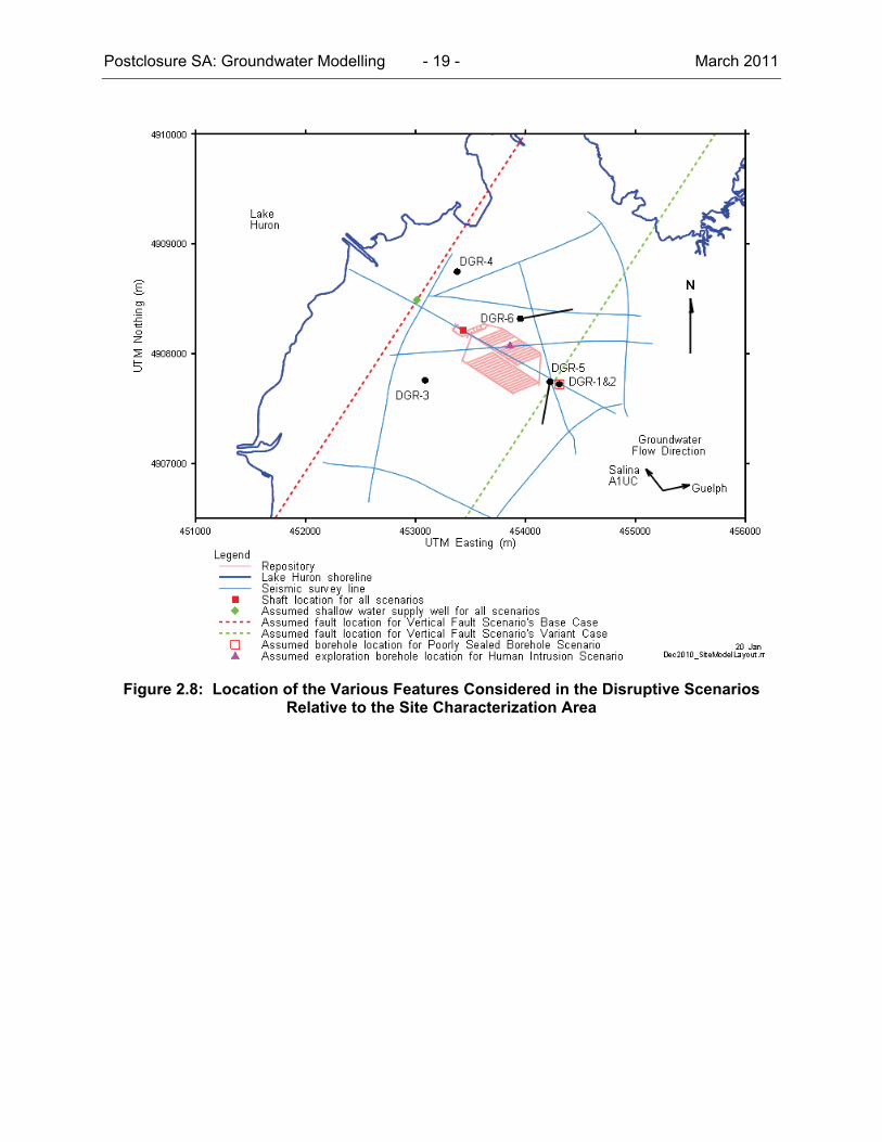
Human Intrusion – An exploration borehole penetrates the repository. The intrusion is assumed to occur once institutional control over the site is no longer effective, and, on closure, the borehole is assumed to be poorly sealed. The case where the borehole is terminated at the repository horizon and where the borehole is continued to the Cambrian will be considered. The assumed location of the borehole is shown in Figure 2.8.
Severe Shaft Seal Failure – The shaft seals (including the EDZ) are assumed to perform much below expectation. That is, the hydraulic conductivities of the seals and EDZ are assumed to be much higher than their design value.
Poorly-Sealed Borehole – A DGR site investigation/monitoring borehole near the repository
is assumed to be poorly sealed on closure. Standard practice is that boreholes that are no longer to be used are sealed with bentonite or cement to prevent contamination of potable water supplies. If this step is improperly performed or the backfill significantly degrades, the closed borehole can provide a preferential path for the migration of contaminated groundwater. The assumed location of the borehole is shown in Figure 2.8.
Vertical Fault – An undetected fault is assumed to exist within the vicinity of the repository.
The permeable vertical fault extends from the Cambrian to the Guelph, and a variety of fault locations must be considered. The assumed locations of the two faults considered in this study are shown in Figure 2.8.
Transient groundwater flow from the observed environmental head profile and contaminant transport modelling was performed to investigate the impact of these Disruptive Scenarios on groundwater flow and contaminant transport. Transient groundwater flow was assumed, because modelling indicated that it would take several million years for the groundwater flow system to equilibrate (i.e., to reach steady state) following the disruption, which is assumed to occur at short time frames before significant radioactive decay. Modelling of the Disruptive Scenarios also indicated that the assumption of steady state flow conditions was not necessarily conservative.
Postclosure SA: Groundwater Modelling - 19 - March 2011
Figure 2.8: Location of the Various Features Considered in the Disruptive Scenarios Relative to the Site Characterization Area

Postclosure SA: Groundwater Modelling - 20 - March 2011
3. CALCULATION CASES
Detailed groundwater modelling was performed for a number of parameter and conceptual model sensitivity cases, over a 1 Ma year time frame, starting at repository closure. All cases were derived from a Reference Case characterization of the system as described in the Data report (QUINTESSA and GEOFIRMA 2011). The Reference Case assumes a constant present-day climate, with no change in boundary conditions during the 1 Ma performance period. Steady state flow is assumed in the Shallow Bedrock Groundwater Zone, while transient flow is assumed in the Intermediate and Deep Bedrock Groundwater Zones.
To make the modelling effort tractable, a number of geometric simplifications were assumed (discussed further in Section 4.3). Some key geometric parameters for the repository are listed here:
7 m high access tunnels and repository; 10 m (immediate) rockfall above access tunnels and repository, where these are
unsupported by concrete, effectively extending the unsupported access tunnels and repository to a height of 17 m;
8.5 m EDZ above, below and on sides of unsupported access tunnels and repository and associated rockfall, with hydraulic conductivity set three orders of magnitude higher than surrounding undisturbed rock;
5 m EDZ above, below and on sides of supported access tunnels (i.e., around concrete monolith); and
HDZ extending 2 m above and below and 0.5 m laterally from supported access tunnels (i.e., concrete monolith), with high hydraulic conductivity.
The shaft geometry was characterized by:
Removal of concrete liner and 0.5 m thick HDZ in the Intermediate and Deep Bedrock Groundwater Zone;
Main and ventilation shaft combined into one shaft with radius of 5.90 m; Below the base of the main shaft the radius was reduced to 3.73 m to represent the deeper
bottom of the ventilation shaft; Shaft sealing materials contained within the 5.9 m or 3.73 m radii (specifically: the concrete
bulkheads do not intercept the shaft inner EDZ); and Inner EDZ thickness was 0.5 times shaft radius, outer EDZ extended beyond the inner EDZ
another 0.5 times the shaft radius.
Boundary conditions for the Reference Case model are as follows:
Zero vertical hydraulic gradient across the Shallow Bedrock Groundwater Zone; Constant horizontal gradient across the Shallow Bedrock Groundwater Zone, inducing flow
towards Lake Huron; Constant pumping from a single well at a rate sufficient for a small farming operation, at a
location 500 m down-flow from the shaft; 165 m hydraulic head fixed boundary at the bottom of the modelled system (the top of the
Cambrian sandstone); 0 m fixed head boundary at the top of the Intermediate Bedrock Groundwater Zone
(implemented at the top of the Salina F formation);
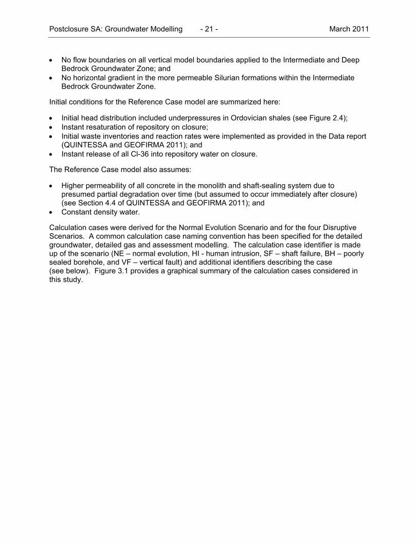
Postclosure SA: Groundwater Modelling - 21 - March 2011
No flow boundaries on all vertical model boundaries applied to the Intermediate and Deep
Bedrock Groundwater Zone; and No horizontal gradient in the more permeable Silurian formations within the Intermediate
Bedrock Groundwater Zone.
Initial conditions for the Reference Case model are summarized here:
Initial head distribution included underpressures in Ordovician shales (see Figure 2.4); Instant resaturation of repository on closure; Initial waste inventories and reaction rates were implemented as provided in the Data report
(QUINTESSA and GEOFIRMA 2011); and Instant release of all Cl-36 into repository water on closure.
The Reference Case model also assumes:
Higher permeability of all concrete in the monolith and shaft-sealing system due to presumed partial degradation over time (but assumed to occur immediately after closure) (see Section 4.4 of QUINTESSA and GEOFIRMA 2011); and
Constant density water.
Calculation cases were derived for the Normal Evolution Scenario and for the four Disruptive Scenarios. A common calculation case naming convention has been specified for the detailed groundwater, detailed gas and assessment modelling. The calculation case identifier is made up of the scenario (NE – normal evolution, HI - human intrusion, SF – shaft failure, BH – poorly sealed borehole, and VF – vertical fault) and additional identifiers describing the case (see below). Figure 3.1 provides a graphical summary of the calculation cases considered in this study.

Pos
tclo
sure
SA
: Gro
und
wat
er M
odel
ling
-22-
M
arch
201
1
Fig
ure
3.1
: S
um
mar
y o
f C
alcu
lati
on
Cas
es C
on
sid
ered

Postclosure SA: Groundwater Modelling - 23 - March 2011
3.1 Normal Evolution Scenario
A number of parameter and conceptual model sensitivity cases have been developed to assess the impact of alternative parameterizations and models of the EDZ, engineered barrier systems, and geosphere. Table 3.1 describes the modelling cases for the Normal Evolution Scenario and the modelling approaches used to simulate those cases. Cases with PD designation are for the final preliminary design, e.g. NE-PD-RC; otherwise the cases are for the original preliminary design – see Figure 2.5.
As noted in Table 3.1, transient flow from the observed underpressured condition (see Figure 2.4) was assumed in case NE-RC. The NE-SBC case was identical to the NE-RC case, but assumed steady state flow (i.e., that the underpressures have dissipated). Steady state flow was also assumed in the remainder of the Normal Evolution cases.
3.2 Disruptive Scenarios
Table 3.2 describes the modelling cases for the Disruptive Scenarios and the modelling approaches used to simulate those cases.
Initial conditions were set to the observed underpressured condition (see Figure 2.4), and transient flow was modelled in all cases.
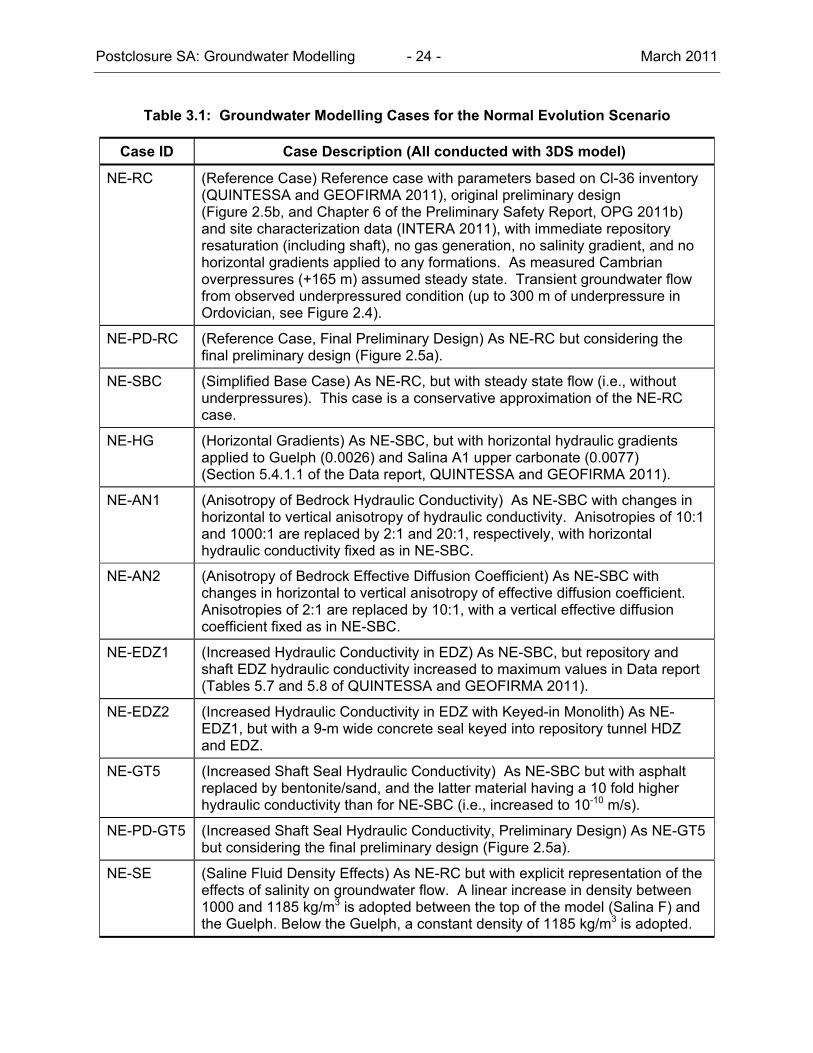
Postclosure SA: Groundwater Modelling - 24 - March 2011
Table 3.1: Groundwater Modelling Cases for the Normal Evolution Scenario
Case ID Case Description (All conducted with 3DS model)
NE-RC (Reference Case) Reference case with parameters based on Cl-36 inventory (QUINTESSA and GEOFIRMA 2011), original preliminary design (Figure 2.5b, and Chapter 6 of the Preliminary Safety Report, OPG 2011b) and site characterization data (INTERA 2011), with immediate repository resaturation (including shaft), no gas generation, no salinity gradient, and no horizontal gradients applied to any formations. As measured Cambrian overpressures (+165 m) assumed steady state. Transient groundwater flow from observed underpressured condition (up to 300 m of underpressure in Ordovician, see Figure 2.4).
NE-PD-RC (Reference Case, Final Preliminary Design) As NE-RC but considering the final preliminary design (Figure 2.5a).
NE-SBC (Simplified Base Case) As NE-RC, but with steady state flow (i.e., without underpressures). This case is a conservative approximation of the NE-RC case.
NE-HG (Horizontal Gradients) As NE-SBC, but with horizontal hydraulic gradients applied to Guelph (0.0026) and Salina A1 upper carbonate (0.0077) (Section 5.4.1.1 of the Data report, QUINTESSA and GEOFIRMA 2011).
NE-AN1 (Anisotropy of Bedrock Hydraulic Conductivity) As NE-SBC with changes in horizontal to vertical anisotropy of hydraulic conductivity. Anisotropies of 10:1 and 1000:1 are replaced by 2:1 and 20:1, respectively, with horizontal hydraulic conductivity fixed as in NE-SBC.
NE-AN2 (Anisotropy of Bedrock Effective Diffusion Coefficient) As NE-SBC with changes in horizontal to vertical anisotropy of effective diffusion coefficient. Anisotropies of 2:1 are replaced by 10:1, with a vertical effective diffusion coefficient fixed as in NE-SBC.
NE-EDZ1 (Increased Hydraulic Conductivity in EDZ) As NE-SBC, but repository and shaft EDZ hydraulic conductivity increased to maximum values in Data report (Tables 5.7 and 5.8 of QUINTESSA and GEOFIRMA 2011).
NE-EDZ2 (Increased Hydraulic Conductivity in EDZ with Keyed-in Monolith) As NE-EDZ1, but with a 9-m wide concrete seal keyed into repository tunnel HDZ and EDZ.
NE-GT5 (Increased Shaft Seal Hydraulic Conductivity) As NE-SBC but with asphalt replaced by bentonite/sand, and the latter material having a 10 fold higher hydraulic conductivity than for NE-SBC (i.e., increased to 10-10 m/s).
NE-PD-GT5 (Increased Shaft Seal Hydraulic Conductivity, Preliminary Design) As NE-GT5 but considering the final preliminary design (Figure 2.5a).
NE-SE (Saline Fluid Density Effects) As NE-RC but with explicit representation of the effects of salinity on groundwater flow. A linear increase in density between 1000 and 1185 kg/m3 is adopted between the top of the model (Salina F) and the Guelph. Below the Guelph, a constant density of 1185 kg/m3 is adopted.
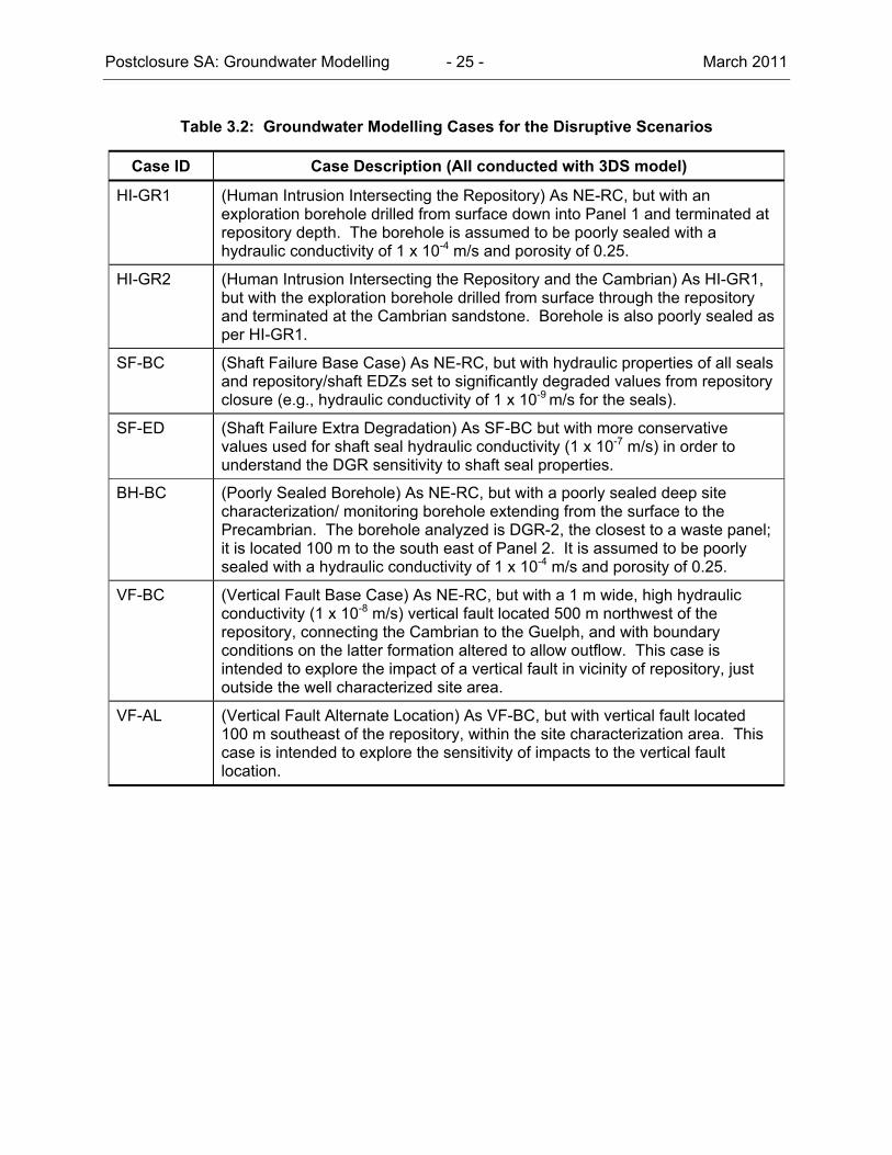
Postclosure SA: Groundwater Modelling - 25 - March 2011
Table 3.2: Groundwater Modelling Cases for the Disruptive Scenarios
Case ID Case Description (All conducted with 3DS model)
HI-GR1 (Human Intrusion Intersecting the Repository) As NE-RC, but with an exploration borehole drilled from surface down into Panel 1 and terminated at repository depth. The borehole is assumed to be poorly sealed with a hydraulic conductivity of 1 x 10⁻⁴ m/s and porosity of 0.25.
HI-GR2 (Human Intrusion Intersecting the Repository and the Cambrian) As HI-GR1, but with the exploration borehole drilled from surface through the repository and terminated at the Cambrian sandstone. Borehole is also poorly sealed as per HI-GR1.
SF-BC (Shaft Failure Base Case) As NE-RC, but with hydraulic properties of all seals and repository/shaft EDZs set to significantly degraded values from repository closure (e.g., hydraulic conductivity of 1 x 10⁻⁹ m/s for the seals).
SF-ED (Shaft Failure Extra Degradation) As SF-BC but with more conservative values used for shaft seal hydraulic conductivity (1 x 10⁻⁷ m/s) in order to understand the DGR sensitivity to shaft seal properties.
BH-BC (Poorly Sealed Borehole) As NE-RC, but with a poorly sealed deep site characterization/ monitoring borehole extending from the surface to the Precambrian. The borehole analyzed is DGR-2, the closest to a waste panel; it is located 100 m to the south east of Panel 2. It is assumed to be poorly sealed with a hydraulic conductivity of 1 x 10⁻⁴ m/s and porosity of 0.25.
VF-BC (Vertical Fault Base Case) As NE-RC, but with a 1 m wide, high hydraulic conductivity (1 x 10⁻⁸ m/s) vertical fault located 500 m northwest of the repository, connecting the Cambrian to the Guelph, and with boundary conditions on the latter formation altered to allow outflow. This case is intended to explore the impact of a vertical fault in vicinity of repository, just outside the well characterized site area.
VF-AL (Vertical Fault Alternate Location) As VF-BC, but with vertical fault located 100 m southeast of the repository, within the site characterization area. This case is intended to explore the sensitivity of impacts to the vertical fault location.

Postclosure SA: Groundwater Modelling - 26 - March 2011
4. MODEL IMPLEMENTATION
4.1 Software Codes and Quality Assurance
All detailed groundwater modelling presented in this report was performed using FRAC3DVS-OPG (Version 1.3.0). FRAC3DVS-OPG (Therrien et al. 2010) is a successor code to FRAC3DVS (Therrien and Sudicky 1996). FRAC3DVS is a three-dimensional numeric model describing subsurface flow and solute transport. It has been used extensively by NWMO for previous flow and transport simulations relating to deep geologic repositories. Quality assurance information for FRAC3DVS-OPG is described in Appendix B.
Model pre- and post- processing was performed using mView 4.03, a proprietary modelling support tool developed by Geofirma Engineering Ltd. Pre-processing procedures consisted primarily of discretization, property assignment, and specification of initial and boundary conditions. Post-processing included all summary calculations and visualizations. mView 4.00A was qualified to Yucca Mountain Project (YMP) Software Quality procedures. Additional capabilities added to mView, since the YMP qualification, were verified in compliance with Geofirma’s internal, ISO 9001 compliant, software development procedure.
The detailed groundwater calculations were conducted to standards specified in the project’s quality plan (QUINTESSA 2010) and the Geofirma Engineering ISO9001-2008 registered Quality Management System. There is a specific Work Instruction (WI), Numeric Modelling, which describes model input file management and archiving using a version control system.
4.2 Model Domains
As noted previously, the time domain extends over a period of 1 Ma years, starting at repository closure.
For the purposes of detailed groundwater modelling, the four groundwater zones identified in Section 2.1 were divided into two separate models: the Three-Dimensional Simplified Upper (3DSU) model and the Three-Dimensional Simplified (3DS) model. The horizontal extents of the two domains relative to the UTM coordinate system and the Lake Huron shoreline are shown in Figure 4.1. The lines of easting and northing indicated on Figure 4.1 indicate the origin of a rotated coordinate system used for the groundwater modelling. The x axis in this coordinate system is oriented parallel to the repository panels access tunnels, 33 degrees south of east. The vertical extents of the two domains are shown in Figure 4.2. Further details of the two models are provided below.
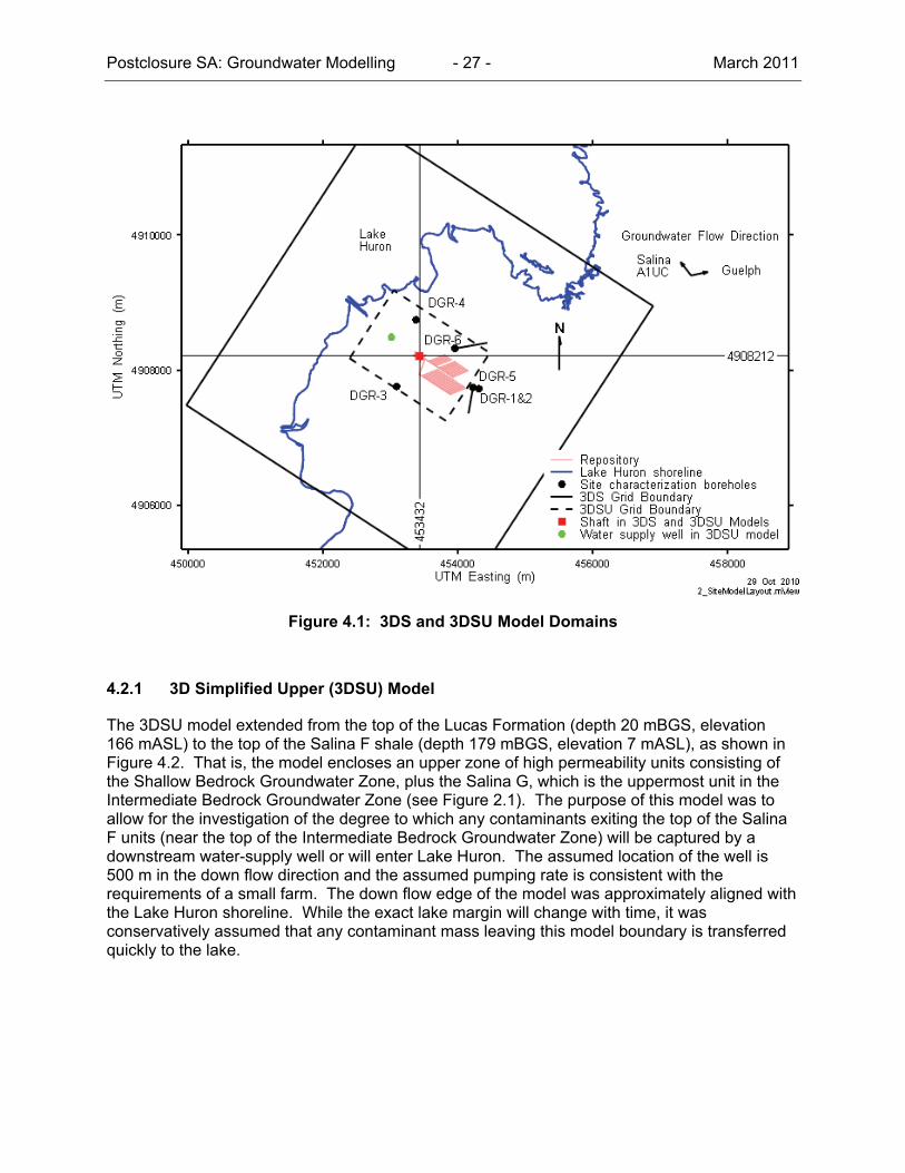
Postclosure SA: Groundwater Modelling - 27 - March 2011
Figure 4.1: 3DS and 3DSU Model Domains
4.2.1 3D Simplified Upper (3DSU) Model
The 3DSU model extended from the top of the Lucas Formation (depth 20 mBGS, elevation 166 mASL) to the top of the Salina F shale (depth 179 mBGS, elevation 7 mASL), as shown in Figure 4.2. That is, the model encloses an upper zone of high permeability units consisting of the Shallow Bedrock Groundwater Zone, plus the Salina G, which is the uppermost unit in the Intermediate Bedrock Groundwater Zone (see Figure 2.1). The purpose of this model was to allow for the investigation of the degree to which any contaminants exiting the top of the Salina F units (near the top of the Intermediate Bedrock Groundwater Zone) will be captured by a downstream water-supply well or will enter Lake Huron. The assumed location of the well is 500 m in the down flow direction and the assumed pumping rate is consistent with the requirements of a small farm. The down flow edge of the model was approximately aligned with the Lake Huron shoreline. While the exact lake margin will change with time, it was conservatively assumed that any contaminant mass leaving this model boundary is transferred quickly to the lake.
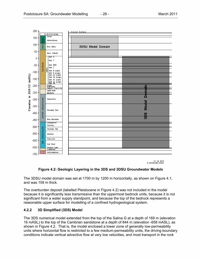
Postclosure SA: Groundwater Modelling - 28 - March 2011
Figure 4.2: Geologic Layering in the 3DS and 3DSU Groundwater Models
The 3DSU model domain was set at 1700 m by 1200 m horizontally, as shown on Figure 4.1, and was 159 m thick.
The overburden deposit (labelled Pleistocene in Figure 4.2) was not included in the model because it is significantly less transmissive than the uppermost bedrock units, because it is not significant from a water supply standpoint, and because the top of the bedrock represents a reasonable upper surface for modelling of a confined hydrogeological system.
4.2.2 3D Simplified (3DS) Model
The 3DS numerical model extended from the top of the Salina G at a depth of 169 m (elevation 16 mASL) to the top of the Cambrian sandstone at a depth of 844 m (elevation -658 mASL), as shown in Figure 4.2. That is, the model enclosed a lower zone of generally low-permeability units where horizontal flow is restricted to a few medium-permeability units, the driving boundary conditions indicate vertical advective flow at very low velocities, and most transport in the rock
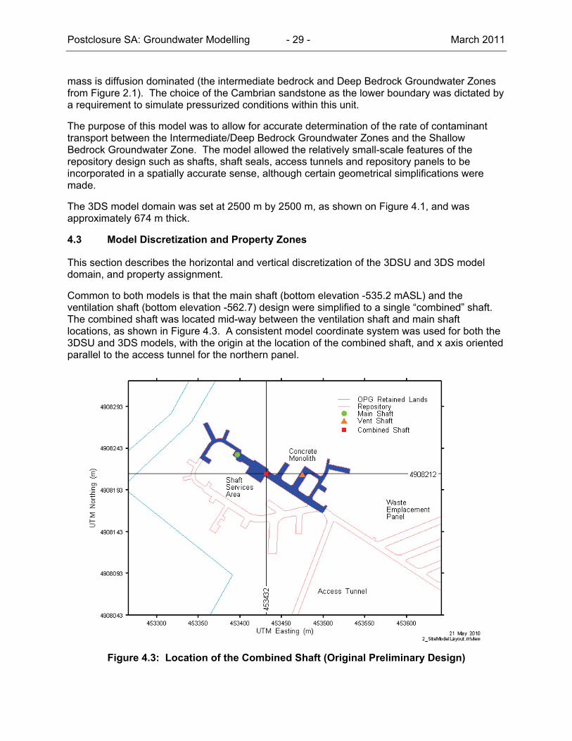
Postclosure SA: Groundwater Modelling - 29 - March 2011
mass is diffusion dominated (the intermediate bedrock and Deep Bedrock Groundwater Zones from Figure 2.1). The choice of the Cambrian sandstone as the lower boundary was dictated by a requirement to simulate pressurized conditions within this unit.
The purpose of this model was to allow for accurate determination of the rate of contaminant transport between the Intermediate/Deep Bedrock Groundwater Zones and the Shallow Bedrock Groundwater Zone. The model allowed the relatively small-scale features of the repository design such as shafts, shaft seals, access tunnels and repository panels to be incorporated in a spatially accurate sense, although certain geometrical simplifications were made.
The 3DS model domain was set at 2500 m by 2500 m, as shown on Figure 4.1, and was approximately 674 m thick.
4.3 Model Discretization and Property Zones
This section describes the horizontal and vertical discretization of the 3DSU and 3DS model domain, and property assignment.
Common to both models is that the main shaft (bottom elevation -535.2 mASL) and the ventilation shaft (bottom elevation -562.7) design were simplified to a single “combined” shaft. The combined shaft was located mid-way between the ventilation shaft and main shaft locations, as shown in Figure 4.3. A consistent model coordinate system was used for both the 3DSU and 3DS models, with the origin at the location of the combined shaft, and x axis oriented parallel to the access tunnel for the northern panel.
Figure 4.3: Location of the Combined Shaft (Original Preliminary Design)
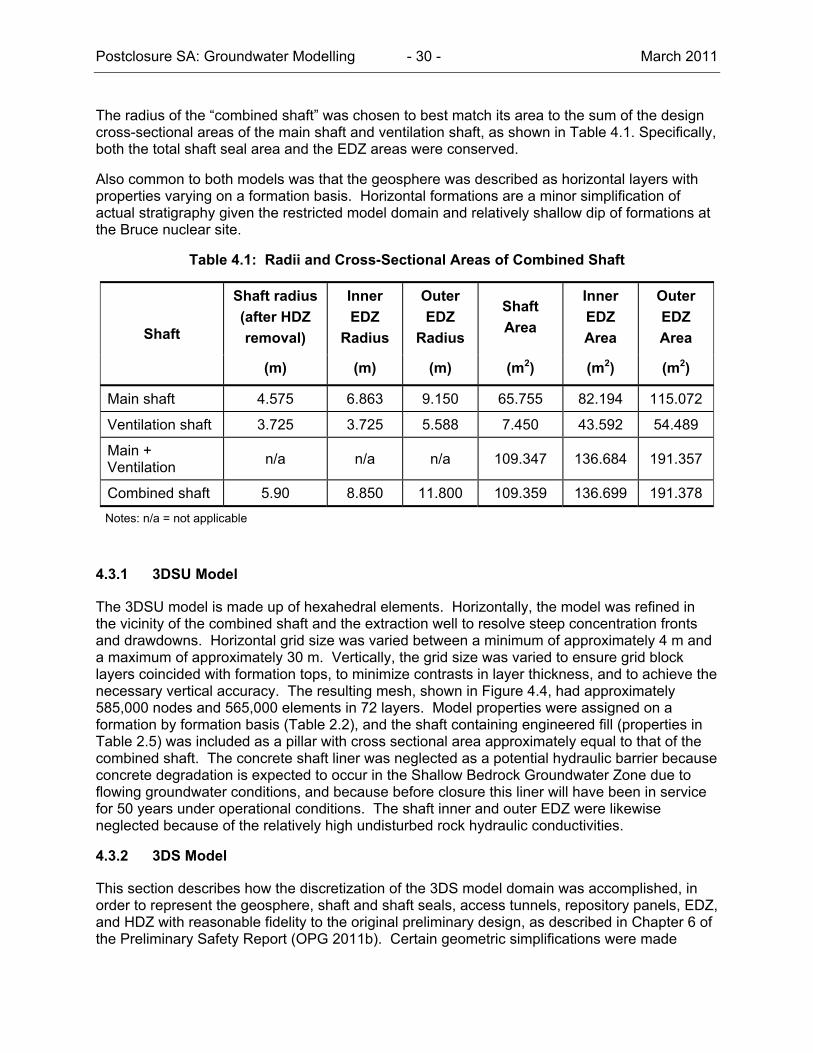
Postclosure SA: Groundwater Modelling - 30 - March 2011
The radius of the “combined shaft” was chosen to best match its area to the sum of the design cross-sectional areas of the main shaft and ventilation shaft, as shown in Table 4.1. Specifically, both the total shaft seal area and the EDZ areas were conserved.
Also common to both models was that the geosphere was described as horizontal layers with properties varying on a formation basis. Horizontal formations are a minor simplification of actual stratigraphy given the restricted model domain and relatively shallow dip of formations at the Bruce nuclear site.
Table 4.1: Radii and Cross-Sectional Areas of Combined Shaft
Shaft
Shaft radius
(after HDZ
removal)
Inner
EDZ
Radius
Outer
EDZ
Radius
Shaft
Area
Inner
EDZ
Area
Outer
EDZ
Area
(m) (m) (m) (m2) (m2) (m2)
Main shaft 4.575 6.863 9.150 65.755 82.194 115.072
Ventilation shaft 3.725 3.725 5.588 7.450 43.592 54.489
Main + Ventilation
n/a n/a n/a 109.347 136.684 191.357
Combined shaft 5.90 8.850 11.800 109.359 136.699 191.378
Notes: n/a = not applicable
4.3.1 3DSU Model
The 3DSU model is made up of hexahedral elements. Horizontally, the model was refined in the vicinity of the combined shaft and the extraction well to resolve steep concentration fronts and drawdowns. Horizontal grid size was varied between a minimum of approximately 4 m and a maximum of approximately 30 m. Vertically, the grid size was varied to ensure grid block layers coincided with formation tops, to minimize contrasts in layer thickness, and to achieve the necessary vertical accuracy. The resulting mesh, shown in Figure 4.4, had approximately 585,000 nodes and 565,000 elements in 72 layers. Model properties were assigned on a formation by formation basis (Table 2.2), and the shaft containing engineered fill (properties in Table 2.5) was included as a pillar with cross sectional area approximately equal to that of the combined shaft. The concrete shaft liner was neglected as a potential hydraulic barrier because concrete degradation is expected to occur in the Shallow Bedrock Groundwater Zone due to flowing groundwater conditions, and because before closure this liner will have been in service for 50 years under operational conditions. The shaft inner and outer EDZ were likewise neglected because of the relatively high undisturbed rock hydraulic conductivities.
4.3.2 3DS Model
This section describes how the discretization of the 3DS model domain was accomplished, in order to represent the geosphere, shaft and shaft seals, access tunnels, repository panels, EDZ, and HDZ with reasonable fidelity to the original preliminary design, as described in Chapter 6 of the Preliminary Safety Report (OPG 2011b). Certain geometric simplifications were made
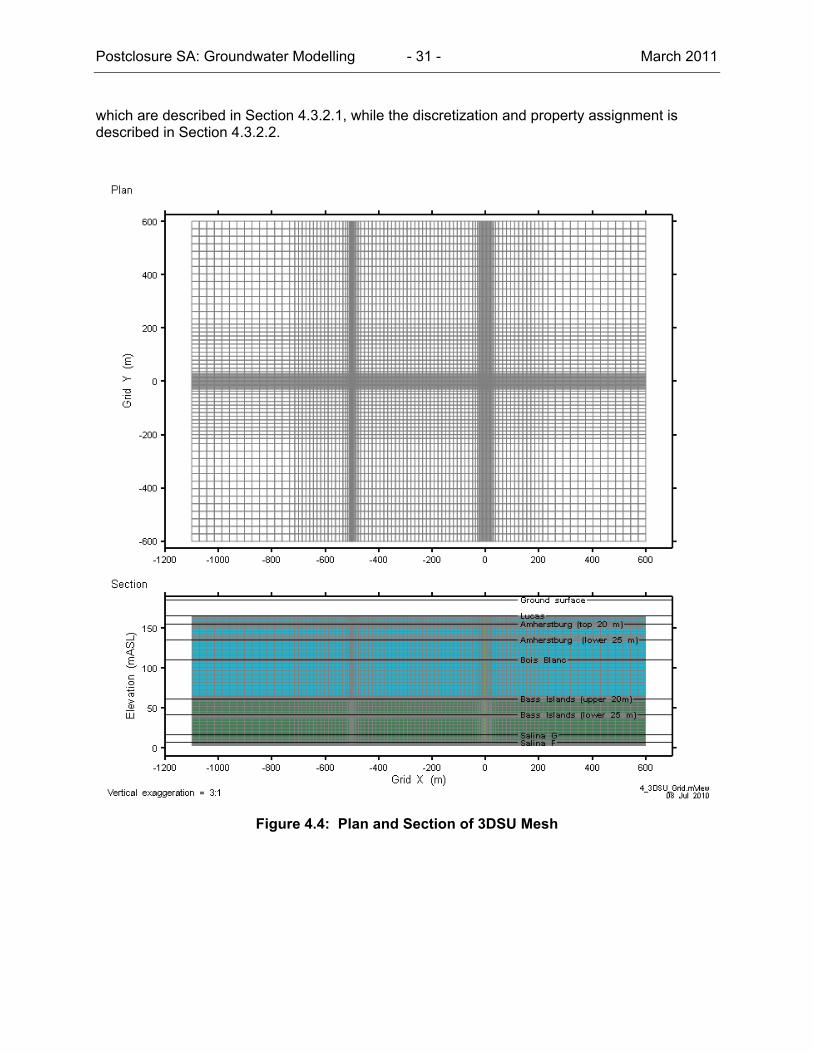
Postclosure SA: Groundwater Modelling - 31 - March 2011
which are described in Section 4.3.2.1, while the discretization and property assignment is described in Section 4.3.2.2.
Figure 4.4: Plan and Section of 3DSU Mesh
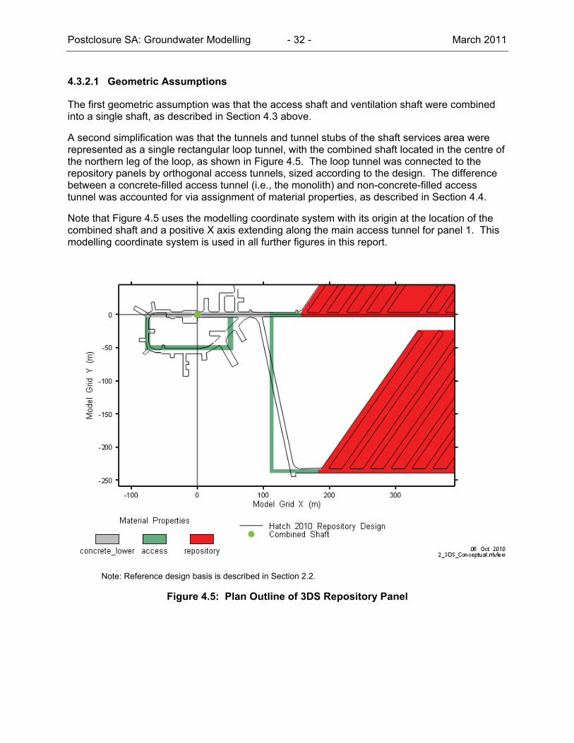
Postclosure SA: Groundwater Modelling - 32 - March 2011
4.3.2.1 Geometric Assumptions
The first geometric assumption was that the access shaft and ventilation shaft were combined into a single shaft, as described in Section 4.3 above.
A second simplification was that the tunnels and tunnel stubs of the shaft services area were represented as a single rectangular loop tunnel, with the combined shaft located in the centre of the northern leg of the loop, as shown in Figure 4.5. The loop tunnel was connected to the repository panels by orthogonal access tunnels, sized according to the design. The difference between a concrete-filled access tunnel (i.e., the monolith) and non-concrete-filled access tunnel was accounted for via assignment of material properties, as described in Section 4.4.
Note that Figure 4.5 uses the modelling coordinate system with its origin at the location of the combined shaft and a positive X axis extending along the main access tunnel for panel 1. This modelling coordinate system is used in all further figures in this report.
Note: Reference design basis is described in Section 2.2.
Figure 4.5: Plan Outline of 3DS Repository Panel
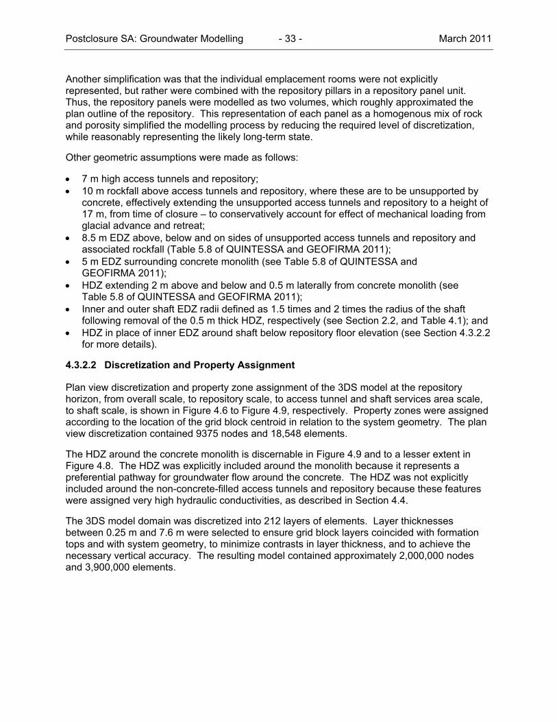
Postclosure SA: Groundwater Modelling - 33 - March 2011
Another simplification was that the individual emplacement rooms were not explicitly represented, but rather were combined with the repository pillars in a repository panel unit. Thus, the repository panels were modelled as two volumes, which roughly approximated the plan outline of the repository. This representation of each panel as a homogenous mix of rock and porosity simplified the modelling process by reducing the required level of discretization, while reasonably representing the likely long-term state.
Other geometric assumptions were made as follows:
7 m high access tunnels and repository; 10 m rockfall above access tunnels and repository, where these are to be unsupported by
concrete, effectively extending the unsupported access tunnels and repository to a height of 17 m, from time of closure – to conservatively account for effect of mechanical loading from glacial advance and retreat;
8.5 m EDZ above, below and on sides of unsupported access tunnels and repository and associated rockfall (Table 5.8 of QUINTESSA and GEOFIRMA 2011);
5 m EDZ surrounding concrete monolith (see Table 5.8 of QUINTESSA and GEOFIRMA 2011);
HDZ extending 2 m above and below and 0.5 m laterally from concrete monolith (see Table 5.8 of QUINTESSA and GEOFIRMA 2011);
Inner and outer shaft EDZ radii defined as 1.5 times and 2 times the radius of the shaft following removal of the 0.5 m thick HDZ, respectively (see Section 2.2, and Table 4.1); and
HDZ in place of inner EDZ around shaft below repository floor elevation (see Section 4.3.2.2 for more details).
4.3.2.2 Discretization and Property Assignment
Plan view discretization and property zone assignment of the 3DS model at the repository horizon, from overall scale, to repository scale, to access tunnel and shaft services area scale, to shaft scale, is shown in Figure 4.6 to Figure 4.9, respectively. Property zones were assigned according to the location of the grid block centroid in relation to the system geometry. The plan view discretization contained 9375 nodes and 18,548 elements.
The HDZ around the concrete monolith is discernable in Figure 4.9 and to a lesser extent in Figure 4.8. The HDZ was explicitly included around the monolith because it represents a preferential pathway for groundwater flow around the concrete. The HDZ was not explicitly included around the non-concrete-filled access tunnels and repository because these features were assigned very high hydraulic conductivities, as described in Section 4.4.
The 3DS model domain was discretized into 212 layers of elements. Layer thicknesses between 0.25 m and 7.6 m were selected to ensure grid block layers coincided with formation tops and with system geometry, to minimize contrasts in layer thickness, and to achieve the necessary vertical accuracy. The resulting model contained approximately 2,000,000 nodes and 3,900,000 elements.
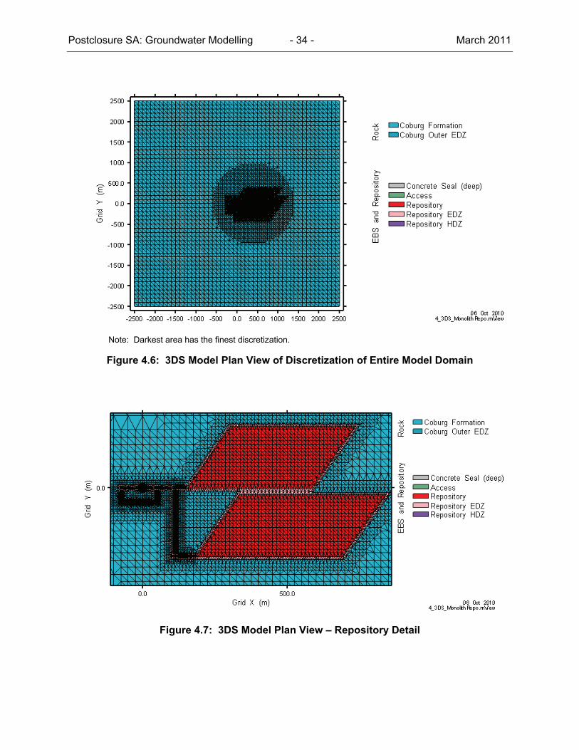
Postclosure SA: Groundwater Modelling - 34 - March 2011
Note: Darkest area has the finest discretization.
Figure 4.6: 3DS Model Plan View of Discretization of Entire Model Domain
Figure 4.7: 3DS Model Plan View – Repository Detail
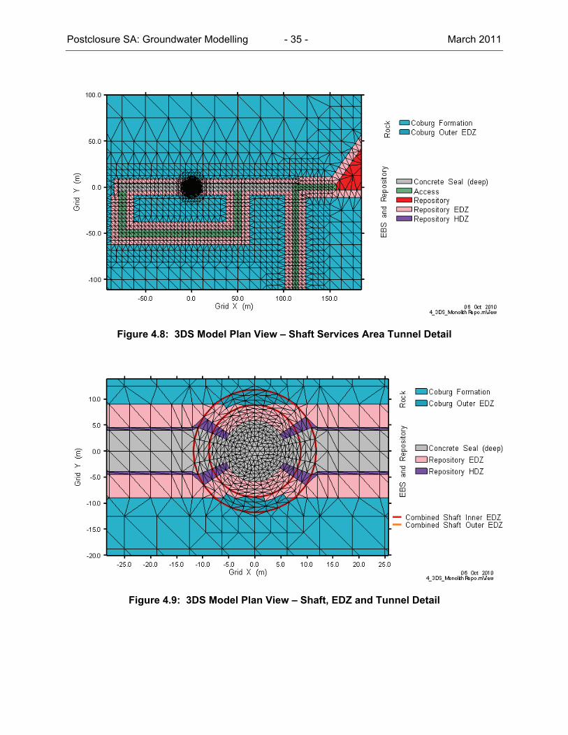
Postclosure SA: Groundwater Modelling - 35 - March 2011
Figure 4.8: 3DS Model Plan View – Shaft Services Area Tunnel Detail
Figure 4.9: 3DS Model Plan View – Shaft, EDZ and Tunnel Detail
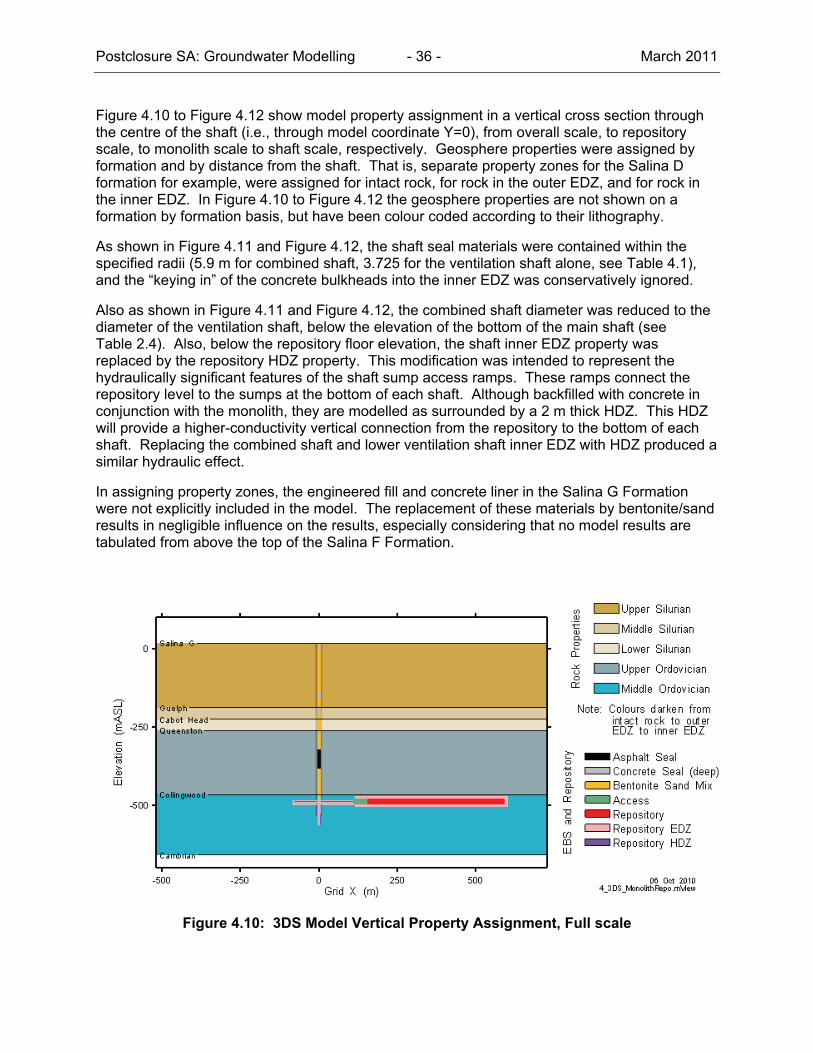
Postclosure SA: Groundwater Modelling - 36 - March 2011
Figure 4.10 to Figure 4.12 show model property assignment in a vertical cross section through the centre of the shaft (i.e., through model coordinate Y=0), from overall scale, to repository scale, to monolith scale to shaft scale, respectively. Geosphere properties were assigned by formation and by distance from the shaft. That is, separate property zones for the Salina D formation for example, were assigned for intact rock, for rock in the outer EDZ, and for rock in the inner EDZ. In Figure 4.10 to Figure 4.12 the geosphere properties are not shown on a formation by formation basis, but have been colour coded according to their lithography.
As shown in Figure 4.11 and Figure 4.12, the shaft seal materials were contained within the specified radii (5.9 m for combined shaft, 3.725 for the ventilation shaft alone, see Table 4.1), and the “keying in” of the concrete bulkheads into the inner EDZ was conservatively ignored.
Also as shown in Figure 4.11 and Figure 4.12, the combined shaft diameter was reduced to the diameter of the ventilation shaft, below the elevation of the bottom of the main shaft (see Table 2.4). Also, below the repository floor elevation, the shaft inner EDZ property was replaced by the repository HDZ property. This modification was intended to represent the hydraulically significant features of the shaft sump access ramps. These ramps connect the repository level to the sumps at the bottom of each shaft. Although backfilled with concrete in conjunction with the monolith, they are modelled as surrounded by a 2 m thick HDZ. This HDZ will provide a higher-conductivity vertical connection from the repository to the bottom of each shaft. Replacing the combined shaft and lower ventilation shaft inner EDZ with HDZ produced a similar hydraulic effect.
In assigning property zones, the engineered fill and concrete liner in the Salina G Formation were not explicitly included in the model. The replacement of these materials by bentonite/sand results in negligible influence on the results, especially considering that no model results are tabulated from above the top of the Salina F Formation.
Figure 4.10: 3DS Model Vertical Property Assignment, Full scale

Postclosure SA: Groundwater Modelling - 37 - March 2011
Figure 4.11: 3DS Model Vertical Property Assignment, Showing Monolith, HDZ, Access Tunnels and Repository
Figure 4.12: 3DS Model Vertical Property Assignment, Showing Shaft Seals, Inner and Outer EDZ, and HDZ below Repository (Horizontal Exaggeration 10:1)
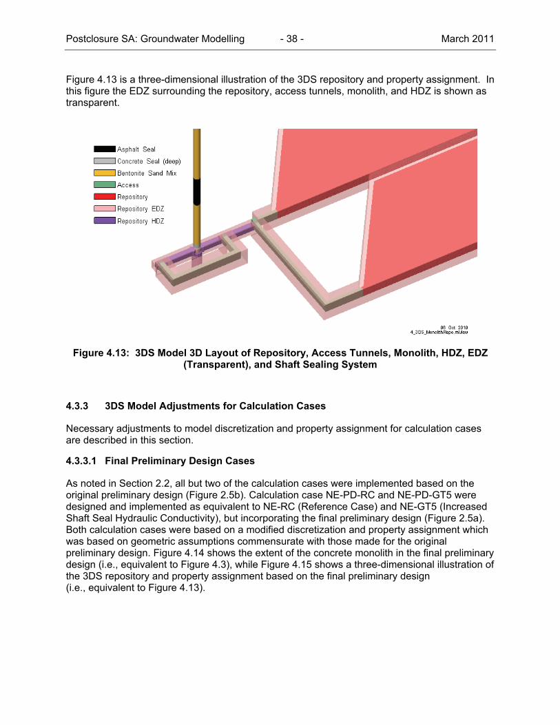
Postclosure SA: Groundwater Modelling - 38 - March 2011
Figure 4.13 is a three-dimensional illustration of the 3DS repository and property assignment. In this figure the EDZ surrounding the repository, access tunnels, monolith, and HDZ is shown as transparent.
Figure 4.13: 3DS Model 3D Layout of Repository, Access Tunnels, Monolith, HDZ, EDZ (Transparent), and Shaft Sealing System
4.3.3 3DS Model Adjustments for Calculation Cases
Necessary adjustments to model discretization and property assignment for calculation cases are described in this section.
4.3.3.1 Final Preliminary Design Cases
As noted in Section 2.2, all but two of the calculation cases were implemented based on the original preliminary design (Figure 2.5b). Calculation case NE-PD-RC and NE-PD-GT5 were designed and implemented as equivalent to NE-RC (Reference Case) and NE-GT5 (Increased Shaft Seal Hydraulic Conductivity), but incorporating the final preliminary design (Figure 2.5a). Both calculation cases were based on a modified discretization and property assignment which was based on geometric assumptions commensurate with those made for the original preliminary design. Figure 4.14 shows the extent of the concrete monolith in the final preliminary design (i.e., equivalent to Figure 4.3), while Figure 4.15 shows a three-dimensional illustration of the 3DS repository and property assignment based on the final preliminary design (i.e., equivalent to Figure 4.13).
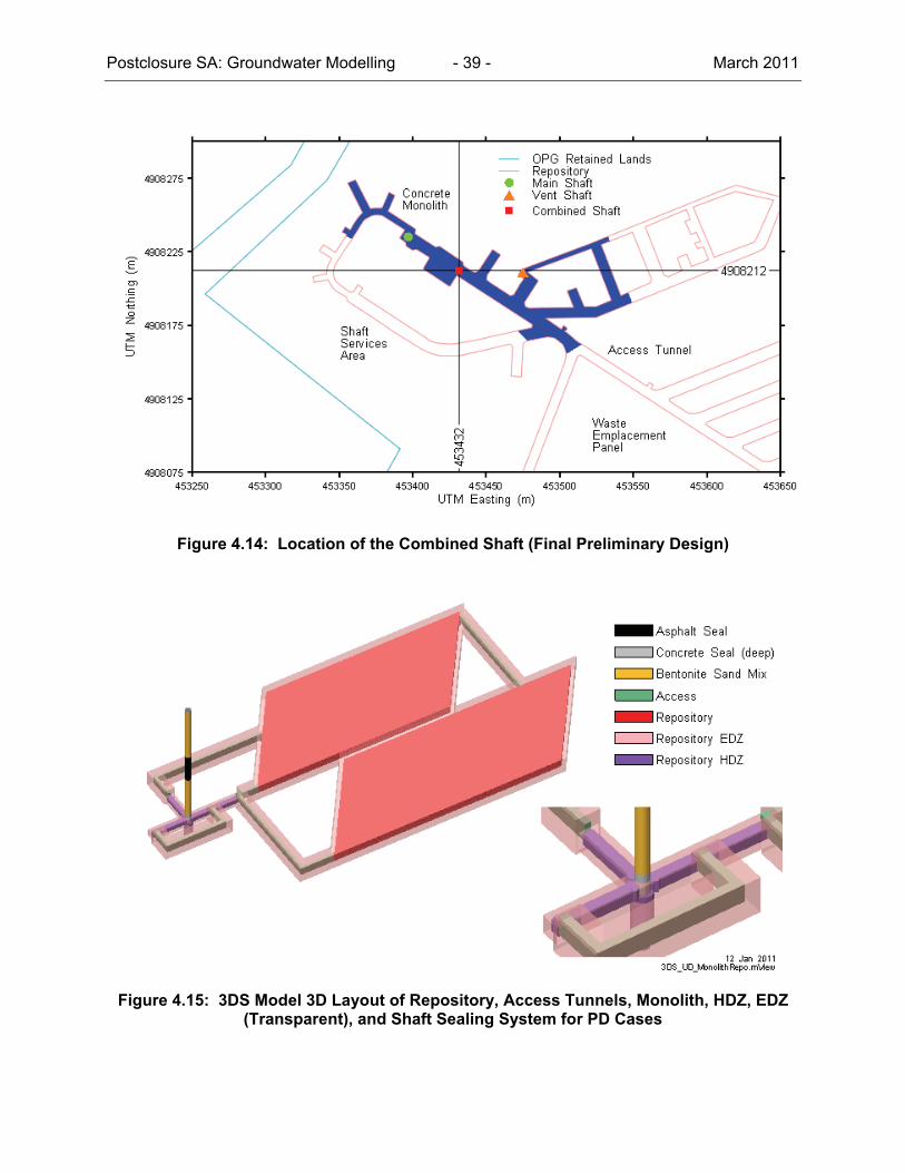
Postclosure SA: Groundwater Modelling - 39 - March 2011
Figure 4.14: Location of the Combined Shaft (Final Preliminary Design)
Figure 4.15: 3DS Model 3D Layout of Repository, Access Tunnels, Monolith, HDZ, EDZ (Transparent), and Shaft Sealing System for PD Cases
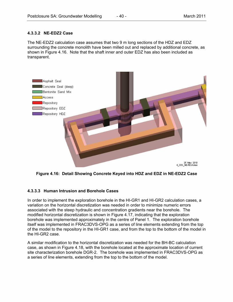
Postclosure SA: Groundwater Modelling - 40 - March 2011
4.3.3.2 NE-EDZ2 Case
The NE-EDZ2 calculation case assumes that two 9 m long sections of the HDZ and EDZ surrounding the concrete monolith have been milled out and replaced by additional concrete, as shown in Figure 4.16. Note that the shaft inner and outer EDZ has also been included as transparent.
Figure 4.16: Detail Showing Concrete Keyed into HDZ and EDZ in NE-EDZ2 Case
4.3.3.3 Human Intrusion and Borehole Cases
In order to implement the exploration borehole in the HI-GR1 and HI-GR2 calculation cases, a variation on the horizontal discretization was needed in order to minimize numeric errors associated with the steep hydraulic and concentration gradients near the borehole. The modified horizontal discretization is shown in Figure 4.17, indicating that the exploration borehole was implemented approximately in the centre of Panel 1. The exploration borehole itself was implemented in FRAC3DVS-OPG as a series of line elements extending from the top of the model to the repository in the HI-GR1 case, and from the top to the bottom of the model in the HI-GR2 case.
A similar modification to the horizontal discretization was needed for the BH-BC calculation case, as shown in Figure 4.18, with the borehole located at the approximate location of current site characterization borehole DGR-2. The borehole was implemented in FRAC3DVS-OPG as a series of line elements, extending from the top to the bottom of the model.
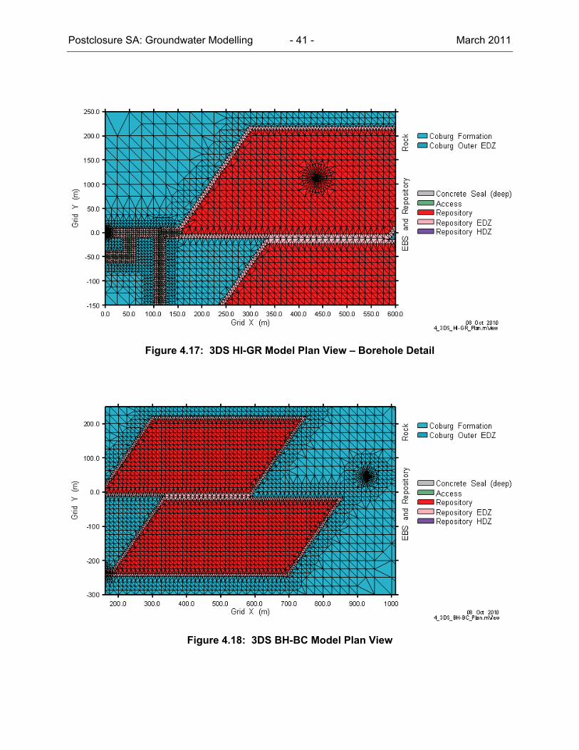
Postclosure SA: Groundwater Modelling - 41 - March 2011
Figure 4.17: 3DS HI-GR Model Plan View – Borehole Detail
Figure 4.18: 3DS BH-BC Model Plan View
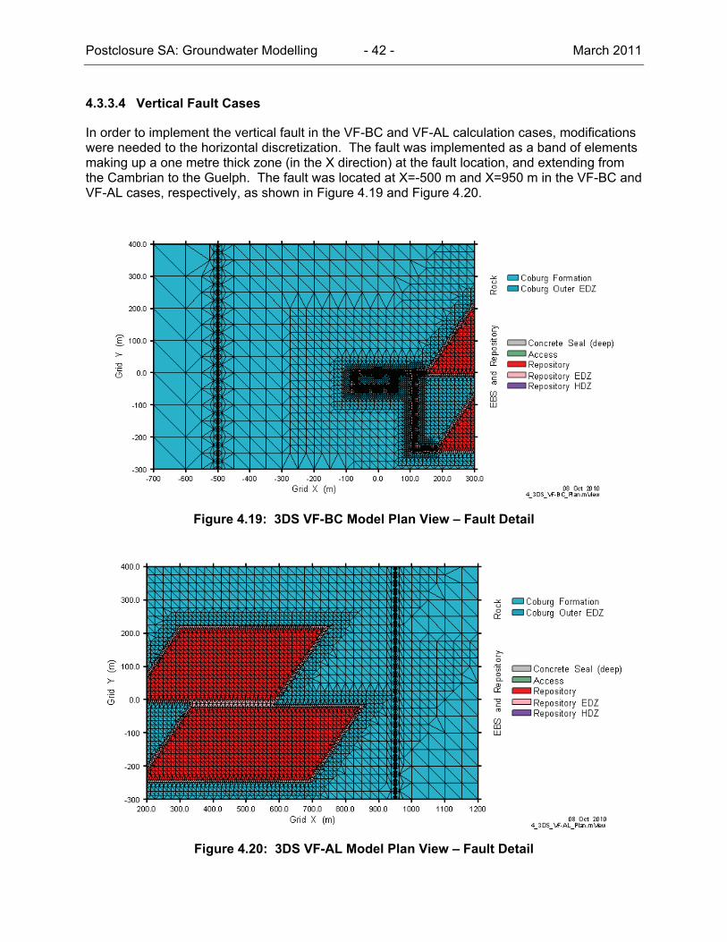
Postclosure SA: Groundwater Modelling - 42 - March 2011
4.3.3.4 Vertical Fault Cases
In order to implement the vertical fault in the VF-BC and VF-AL calculation cases, modifications were needed to the horizontal discretization. The fault was implemented as a band of elements making up a one metre thick zone (in the X direction) at the fault location, and extending from the Cambrian to the Guelph. The fault was located at X=-500 m and X=950 m in the VF-BC and VF-AL cases, respectively, as shown in Figure 4.19 and Figure 4.20.
Figure 4.19: 3DS VF-BC Model Plan View – Fault Detail
Figure 4.20: 3DS VF-AL Model Plan View – Fault Detail
Postclosure SA: Groundwater Modelling - 43 - March 2011
4.3.4 Discretization of Time
The 1 Ma performance period was discretized into steadily increasing time steps, for simulation of transient groundwater flow and/or solute transport. The starting time step in all simulations was set at 0.01 seconds, and the time step multiplier was calculated by FRAC3DVS-OPG based on allowable increases in either hydraulic head (transient flow simulations only) or Cl-36 concentration. The final time step was typically in the order of 25,000 years.
4.4 Contaminant and Material Properties
4.4.1 Contaminant Properties
As noted in Section 1.1, the detailed groundwater modelling assessed results for a single reference contaminant, Cl-36. Radioactive decay of Cl-36 was accounted for in FRAC3DVS-OPG by assignment of a half life of 3.01 x 10⁵ a, as reported in Table 3.12 of QUINTESSA and GEOFIRMA (2011). Sorption of Cl-36 was not considered (see Tables 4.25 and 5.13 of QUINTESSA and GEOFIRMA 2011).
Diffusion of Cl-36 was considered through the specification of effective diffusion coefficients for each material included within the model. Effective diffusion coefficients for the geosphere and for the shaft sealing materials are included in Table 2.2 and Table 2.5, respectively. Effective diffusion coefficients for disturbed rock and underground excavations are detailed in Section 4.4.2. In order to specify effective diffusion coefficient in FRAC3DVS-OPG, a nominal value for free water diffusion coefficient of 1 x 10⁻⁹ m2/s was used, and tortuosities were calculated as described in Appendix C.
4.4.2 Material Properties Used in the Reference (NE-RC Case)
Parameters used by FRAC3DVS-OPG in the detailed groundwater modelling include: porosity, hydraulic conductivity in both the horizontal and vertical directions, effective diffusion coefficient in the horizontal and vertical directions, and specific storage. These values for the undisturbed geosphere and for the shaft sealing materials are summarized in Table 2.2 and in Table 2.5, respectively. The values for the disturbed rock (shaft inner and outer EDZ, monolith HDZ, access tunnel and repository EDZ), and underground excavations are summarized in Table 4.2. It is noted that hydraulic conductivity and effective diffusion coefficient are assumed to be isotropic (same in vertical and horizontal directions) for all the materials covered in the table.
Disturbed rock porosities, hydraulic conductivities, and effective diffusion coefficients in Table 4.2 were calculated relative to the value for undisturbed rock. For example, the hydraulic conductivities for the shaft inner and outer EDZ, were calculated on a formation-by-formation basis, by multiplying the host rock formation vertical hydraulic conductivity (Kz) by 100 times and by 10 times, respectively. This modification reflects the hydromechanical modifications induced by the shaft opening. Since the access tunnels and repository are to be located in the Cobourg Formation, it is useful to restate the relevant values here: porosity of 0.015, horizontal hydraulic conductivity, Kxy, of 1 x 10-14 m/s, vertical hydraulic conductivity, Kz, of 1 x 10-15 m/s, horizontal effective diffusion coefficient, De,xy, of 7.4 x 10⁻¹³ m2/s, and vertical effective diffusion coefficient De,z, of 3.7 x 10⁻¹³ m2/s.
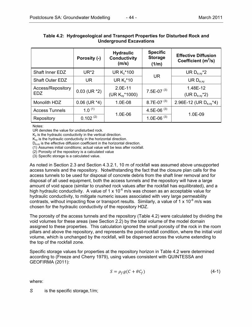
Postclosure SA: Groundwater Modelling - 44 - March 2011
Table 4.2: Hydrogeological and Transport Properties for Disturbed Rock and Underground Excavations
Porosity (-)
Hydraulic Conductivity
(m/s)
Specific Storage
(1/m)
Effective Diffusion Coefficient (m2/s)
Shaft Inner EDZ UR*2 UR Kz*100 UR
UR De,xy*2
Shaft Outer EDZ UR UR Kz*10 UR De,xy
Access/Repository EDZ 0.03 (UR *2)
2.0E-11
(UR Kxy*1000) 7.5E-07 (3)
1.48E-12
(UR De,xy*2)
Monolith HDZ 0.06 (UR *4) 1.0E-08 8.7E-07 (3) 2.96E-12 (UR De,xy*4)
Access Tunnels 1.0 (1) 1.0E-06
4.5E-06 (3) 1.0E-09
Repository 0.102 (2) 1.0E-06 (3)
Notes: UR denotes the value for undisturbed rock. Kz is the hydraulic conductivity in the vertical direction. Kxy is the hydraulic conductivity in the horizontal direction. De,xy is the effective diffusion coefficient in the horizontal direction. (1) Assumes initial conditions; actual value will be less after rockfall. (2) Porosity of the repository is a calculated value (3) Specific storage is a calculated value.
As noted in Section 2.3 and Section 4.3.2.1, 10 m of rockfall was assumed above unsupported access tunnels and the repository. Notwithstanding the fact that the closure plan calls for the access tunnels to be used for disposal of concrete debris from the shaft liner removal and for disposal of all used equipment, both the access tunnels and the repository will have a large amount of void space (similar to crushed rock values after the rockfall has equilibrated), and a high hydraulic conductivity. A value of 1 x 10⁻⁶ m/s was chosen as an acceptable value for hydraulic conductivity, to mitigate numeric issues associated with very large permeability contrasts, without impacting flow or transport results. Similarly, a value of 1 x 10⁻⁸ m/s was chosen for the hydraulic conductivity of the repository HDZ.
The porosity of the access tunnels and the repository (Table 4.2) were calculated by dividing the void volumes for these areas (see Section 2.2) by the total volume of the model domain assigned to these properties. This calculation ignored the small porosity of the rock in the room pillars and above the repository, and represents the post-rockfall condition, where the initial void volume, which is unchanged by the rockfall, will be dispersed across the volume extending to the top of the rockfall zone.
Specific storage values for properties at the repository horizon in Table 4.2 were determined according to (Freeze and Cherry 1979), using values consistent with QUINTESSA and GEOFIRMA (2011):
(4-1)
where:
S is the specific storage,1/m;
Postclosure SA: Groundwater Modelling - 45 - March 2011
f is the fluid density (set at 1185), kg/m3;
g is the gravitational acceleration (set at 9.81), m/s2;
C is the porous medium compressibility (set at 5.5 x 10⁻¹¹), 1/Pa;
is the porosity, unitless; and
Cf is the fluid compressibility (set at 3.3 x 10⁻¹⁰), 1/Pa.
Longitudinal dispersivities for all 3DS model units were set to 10 m, as approximately several percent of the expected plume size over the performance period. Transverse dispersivities were set at 10% of longitudinal dispersivity, or 1 m. Dispersivities in the Devonian system for the 3DSU model were set at 100 m (longitudinal) and 10 m (transverse) to reflect the larger transport distance.
4.4.3 Material Properties Used in Other Calculation Cases
For the NE-EDZ1 calculation case, the shaft inner and outer EDZ hydraulic conductivities were calculated on a formation-by-formation basis, by multiplying the undisturbed rock formation vertical hydraulic conductivity (Kz) by 10,000 times and by 100 times, respectively. The respective multipliers in the NE-RC calculation case were 1000 and 10, respectively (see Table 4.2). Also for the NE-EDZ1 calculation case, the hydraulic conductivity of the access tunnel and repository EDZ was set as 2 x 10⁻¹⁰ m/s, which is a multiplier on the host rock horizontal hydraulic conductivity of 10,000 (relative to 1000 for the NE-RC calculation case). All other parameters were set equal to those of the NE-RC calculation case.
For the SF-BC case all parameters were set as for the NE-EDZ1 case, and the shaft sealing materials (asphalt, concrete, and bentonite/sand) were uniformly given a hydraulic conductivity of 1 x 10⁻⁹ m/s, a porosity of 0.3, and an effective diffusion coefficient of 3 x 10⁻¹⁰ m2/s, to represent significant degradation of these materials.
For the SF-ED case, all parameters were set as for the SF-BC case, but the shaft sealing materials were uniformly given a hydraulic conductivity of 1 x 10⁻⁷ m/s, to represent further degradation of these materials.
For the NE-AN1 calculation case, vertical hydraulic conductivities for the undisturbed rock were adjusted from the NE-RC case (see Table 2.2) as follows. Anisotropies (ratio of horizontal to vertical hydraulic conductivities) of 10:1 were replaced with 2:1; anisotropies of 1000:1 were replaced with 20:1.
For the NE-AN2 calculation case, the ratio of horizontal to vertical effective diffusion coefficient for the undisturbed rock were increased from 2:1 to 10:1, with the vertical effective diffusion coefficient remaining fixed as in the NE-RC calculation case.
The boreholes in the HI-GR1 and HI-GR2 calculation cases was implemented with line elements with properties consistent with a 16.5 cm (6.5 inch) diameter borehole, filled with relatively high hydraulic conductivity material. The properties of the engineered fill (Table 2.5) were assigned to these line elements. In the HI-GR1 calculation case, these line elements extended from the top of the model to the top of the repository. In the HI-GR2 calculation case, the line elements extended from the top to the bottom of the model.
Postclosure SA: Groundwater Modelling - 46 - March 2011
The borehole in the BH-BC calculation case was implemented with line elements extending from the top to the bottom of the model, with properties consistent with a 14.25 cm (5.625 inch) diameter borehole, filled with high hydraulic conductivity material. The properties of the engineered fill (Table 2.5) were assigned to these line elements. Actual closure plans for DGR-2 have not yet been developed, but would involve closure with much lower conductivity material (bentonite or cement) than used in this conservative case.
The one metre thick geologic fault in the VF-BC case was assigned a hydraulic conductivity of 1 x 10⁻⁸ m/s, a porosity of 0.1, specific storage of 1.8 x 10⁻⁵ 1/m, vertical effective diffusion coefficient of 2.3 x 10⁻¹² m2/s, and horizontal effective diffusion coefficient of 4.6 x 10⁻¹² m2/s. The hydraulic conductivity and porosity values are best estimates of the properties of the disturbed rock within the fault zone. The specific storage and effective diffusion coefficients are average values for the formations assumed to be intersected by the fault (Shadow Lake to Goat Island).
4.5 Boundary and Initial Conditions
4.5.1 Boundary Conditions Used in the Reference (NE-RC) Case
The 3DS model was implemented with fixed head boundary conditions on the top and bottom layers of the model, defining a vertical gradient in the system. All modelling cases applied a 165 m total change in head, with the top model surface (at 16 mASL) having a defined head of 0 m, and the bottom surface (at -653 mASL) having a defined head of 165 m.
The value of zero at the top of the Salina G assumes no substantial vertical gradients in the Shallow Bedrock Groundwater Zone. The value of 165 m represents the environmental head calculated from measured Cambrian overpressures, presented previously in Figure 2.4. As noted in Section 2.3, the use of this environmental head as a boundary condition allowed for the use of constant density groundwater in the numerical flow models, as described in Appendix A. It is noted that these boundary conditions define hydraulic head with datum at the ground surface.
All lateral exterior boundaries to the 3DS model were specified as zero flow, implying vertical flow.
In the 3DSU model, a horizontal head gradient of 0.003 (Section 5.4.1.1, QUINTESSA and GEOFIRMA 2011), was imposed with flow direction oriented towards Lake Huron (the negative X direction, in model coordinates). The hydraulic gradient was applied via the specification of fixed hydraulic heads on the up-gradient and down-gradient boundaries, and no-flow boundary conditions on the cross-gradient sides. The imposed gradient corresponds to a head differential of 5.2 m over the 1700 m length. Zero flow was specified on the bottom boundary since upwards groundwater inflow from the Intermediate Bedrock Groundwater Zone, including from the sealed shaft, will be negligible relative to the horizontal flow through the shallow bedrock groundwater system. Zero flow was specified on the upper boundary to be conservative with respect to dilution of the contaminant mass by recharge (recharge is currently low, but could be higher under future conditions).
The 3DSU model required the implementation of a boundary condition to represent a water supply well that will be taking water out of the Shallow Bedrock Groundwater Zone. The water supply well was implemented as a series of constant groundwater flow boundary conditions
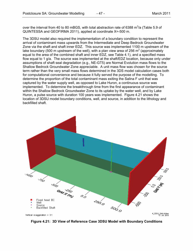
Postclosure SA: Groundwater Modelling - 47 - March 2011
over the interval from 40 to 80 mBGS, with total abstraction rate of 6388 m3/a (Table 5.9 of QUINTESSA and GEOFIRMA 2011), applied at coordinate X=-500 m.
The 3DSU model also required the implementation of a boundary condition to represent the arrival of contaminant mass upwards from the Intermediate and Deep Bedrock Groundwater Zone via the shaft and shaft inner EDZ. This source was implemented 1100 m upstream of the lake boundary (500 m upstream of the well), with a plan view area of 256 m2 (approximately equal to the area of the combined shaft and inner EDZ, see Table 4.1), and a specified mass flow equal to 1 g/a. The source was implemented at the shaft/EDZ location, because only under assumptions of shaft seal degradation (e.g., NE-GT5) are Normal Evolution mass flows to the Shallow Bedrock Groundwater Zone appreciable. A unit mass flow was chosen for the source term rather than the very small mass flows determined in the 3DS model calculation cases both for computational convenience and because it fully served the purpose of the modelling. To determine the proportion of the total contaminant mass exiting the Salina F unit that was captured by the water supply well, as opposed to Lake Huron, a continuous source was implemented. To determine the breakthrough time from the first appearance of contaminant within the Shallow Bedrock Groundwater Zone to its uptake by the water well, and by Lake Huron, a pulse source with duration 100 years was implemented. Figure 4.21 shows the location of 3DSU model boundary conditions, well, and source, in addition to the lithology and backfilled shaft.
Figure 4.21: 3D View of Reference Case 3DSU Model with Boundary Conditions
Postclosure SA: Groundwater Modelling - 48 - March 2011
4.5.2 Initial Conditions Specified in the Reference (NE-RC) Case
The NE-RC calculation case was a transient groundwater flow model and required the specification of an initial hydraulic head distribution. The environmental head profile presented in Figure 2.4 was used for this purpose.
The reference radionuclide Cl-36 source term was defined by specifying an initial concentration for all repository elements. The initial concentration was calculated by assuming that the entire radionuclide inventory of Cl-36 is instantly dissolved at closure. The inventory activity of Cl-36 was converted to a mass and divided by the void volume of the repository in the numeric model to obtain the initial concentration. Using data in Tables 3.15, 3.16 and 4.2 of QUINTESSA and GEOFIRMA (2011), the Cl-36 activity in Panels 1 and 2 will be 9.45 x 10¹¹ Bq and 4.73 x 10¹¹ Bq, respectively. These values correspond to masses of 0.77 kg and 0.39 kg, for Panels 1 and 2, respectively, and source concentrations of 5 x 10⁻³ g/m3 and 2 x 10⁻³ g/m3, respectively, based on the respective panel void volumes (approximately 155,000 m3 in Panel 1, and 199,000 m3 in Panel 2 for a total of 353,000 m3, see Table 4.5 in QUINTESSA and GEOFIRMA 2011). Outside of the repository, the initial Cl-36 concentration was set to zero.
4.5.3 Boundary and Initial Conditions Used in Other Calculation Cases
The NE-HG calculation case required the specification of a hydraulic gradient across the moderately permeable Salina A1 Upper Carbonate and Guelph formations. This hydraulic gradient was specified via constant hydraulic heads applied to the outside nodes of the model, in elements representing these two formations. The values of the constant heads were determined using a two-step process. In the first step, the simulated steady state hydraulic head at the centre of the model in each of these two formations in the absence of any deep geological repository was determined in a separate model run. In the second step, the hydraulic head at the model boundaries was calculated by interpolation according to the assumed hydraulic gradient (see Section 2.1).
In the VF-BC and VF-AL cases, the hydraulic head for all exterior nodes within elements representing the Guelph Formation were set at 7 m above ground surface (mAGS) (the calculated steady state head for this formation). The modification from the no-flow boundary condition used in the NE-RC case was necessary to allow for the discharge of water flowing into the Guelph Formation from the introduced vertical fault.
The NE-SE case required the specification of an initial density profile. Based on the measured density profile presented in Figure 2.3, a linear increase in density between 1000 and 1185 g/m3 was specified between the top of the model and the Guelph formation. Below the Guelph formation, a constant density of 1185 g/m3 was specified.
4.6 Audit of Features, Events and Processes
The Features, Events and Processes (FEPs) report (QUINTESSA et al. 2011b) presents a comprehensive review and screening of FEPs that are relevant to the conceptual models developed for the Normal Evolution and Disruptive Scenarios. Appendix D presents an audit of the FEPs to indicate which FEPs are addressed in the detailed groundwater flow and transport modelling presented in this report and which are excluded. Reasons for exclusion are given and include: limitations in FRAC3DVS-OPG’s ability to represent the FEP; simplifications in modelling approach in the FRAC3DVS-OPG models; and included in assessment modelling using AMBER rather than detailed groundwater modelling using FRAC3DVS-OPG.

Postclosure SA: Groundwater Modelling - 49 - March 2011
5. RESULTS FOR THE NORMAL EVOLUTION SCENARIO
Section 5.1 provides a discussion of formats used for presentation of the results of the detailed groundwater modelling. The results for the Normal Evolution Scenario are presented in the remaining parts of Chapter 5. The discussion of Section 5.1 is also applicable to the results for the Disruptive Scenarios, presented in Chapter 6. Most analyses were conducted for the original preliminary design; specific cases marked with PD were conducted for the final preliminary design for comparison.
5.1 Results Presentation
Within the body of the report, results are presented in graphical format using a variety of visualization approaches. Flow rates required for the assessment level modelling were tabulated and provided under separate cover. Where possible, results presentations are limited to the data ranges that are physically relevant. However, in some cases it was necessary to present very low flow and concentration results to allow effective comparison of different case results.
5.1.1 Flow Results
Flow results are reported largely through the use of hydraulic head and advective linear velocity contour plots.
Hydraulic head ranges and contours are adjusted to best display the data being presented, while maintaining consistency among comparable figures. For example, vertical cross-section plots of the entire model domain will generally show a hydraulic head range of 0 to 165 m with contours at 5 m intervals for steady state results, and a hydraulic head range of -300 to 165 m with contours at 20 m intervals for transient results. Plan view contour plots of hydraulic head at the repository horizon show ranges in head and contour interval which are specific to the case being presented. This is because of a large case by case variation in hydraulic head. As stated in Section 4.5.1, hydraulic head is defined with datum at the ground surface. That is, hydraulic heads greater than zero imply overpressured conditions, while hydraulic heads less than zero imply underpressured conditions, relative to hydrostatic.
Advective linear velocities are generally mapped to a logarithmic colour scale over the range from 1 x 10⁻⁸ to 1 x 10⁻² m/a. Values outside this range are portrayed with the colour associated with maximum or minimum as appropriate. Some figures will have an expanded range if necessary. For most advective velocity figures presented in this report, velocity vectors are shown only for those regions where velocities exceed 10-4 m/a (i.e., at least 100 m of advective transport in 1 Ma). In general, the vector length is scaled by log velocity; however, the scaling factor varies depending upon figure scale, and vector lengths should be regarded as a qualitative indication only.
Horizontal flow rates between the repository and the shaft within the specific zones shown in Figure 5.1 were required for the assessment modelling. Vertical groundwater flow rates within the shaft and the inner and outer shaft EDZ at the specific locations shown in Figure 5.2 were also required for the assessment modelling. These flow rates were determined by multiplying the mean Darcy flux within the zone (either steady state or at specific times, depending on case) by the cross sectional area of the zone. Flows within a 500 m long section of the vertical fault centered on Y=0 for the VF-BC and VF-AL cases were determined in a similar manner.

Postclosure SA: Groundwater Modelling - 50 - March 2011
Figure 5.1: Location of Zones for Tabulation of Horizontal Groundwater Flows
Groundwater flows within boreholes for the HI-GR1, HI-GR2 and BH-BC cases were also required for the assessment level modelling, between the Cambrian and the repository (HI-GR2 only), between the repository elevation and the Guelph, between the Guelph and the Salina A1 Upper Carbonate, and above the Salina A1 Upper Carbonate. These flows were determined by multiplying the hydraulic gradient calculated from model-calculated hydraulic heads, by the cross sectional area of the borehole, by the hydraulic conductivity of the borehole.
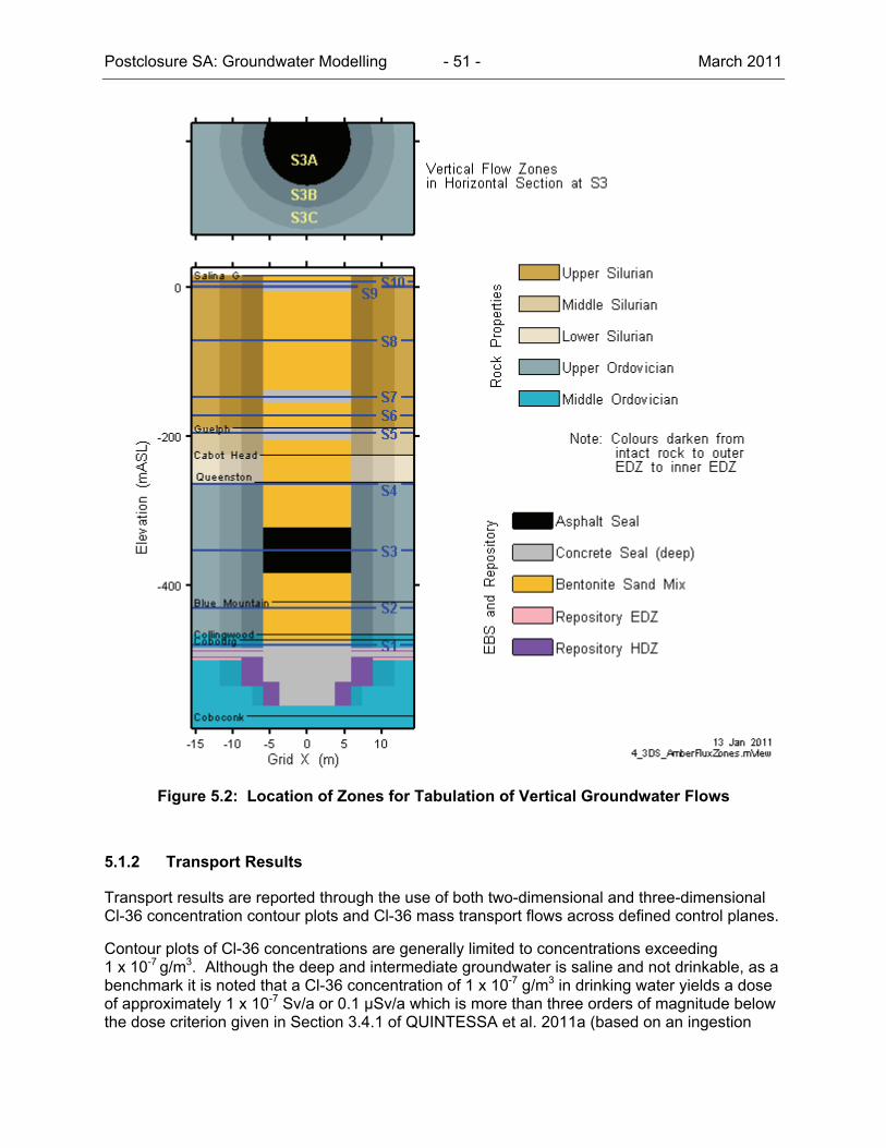
Postclosure SA: Groundwater Modelling - 51 - March 2011
Figure 5.2: Location of Zones for Tabulation of Vertical Groundwater Flows
5.1.2 Transport Results
Transport results are reported through the use of both two-dimensional and three-dimensional Cl-36 concentration contour plots and Cl-36 mass transport flows across defined control planes.
Contour plots of Cl-36 concentrations are generally limited to concentrations exceeding 1 x 10⁻⁷ g/m3. Although the deep and intermediate groundwater is saline and not drinkable, as a benchmark it is noted that a Cl-36 concentration of 1 x 10⁻⁷ g/m3 in drinking water yields a dose of approximately 1 x 10⁻⁷ Sv/a or 0.1 µSv/a which is more than three orders of magnitude below the dose criterion given in Section 3.4.1 of QUINTESSA et al. 2011a (based on an ingestion
Postclosure SA: Groundwater Modelling - 52 - March 2011
rate of 2.3 L/d and a dose coefficient of 9.3 x 10⁻¹⁰ Sv/Bq, Table 7.7 of QUINTESSA and GEOFIRMA 2011).
Graphs of Cl-36 mass flow versus time are generally limited to 1 x 10-14 g/a and above. As a benchmark it is noted that Cl-36 is produced naturally in the atmosphere, and that the global average deposition rate is approximately 10 atoms/m2s (Fritz and Fontes 1986). Over the approximately 0.25 km2 panel footprint of the DGR (Table 4.3, QUINTESSA and GEOFIRMA 2011), this deposition rate translates to 5 x 10⁻⁹ g/a. Given that the atmospheric Cl-36 deposition rate is latitude dependent and is likely higher in southern Ontario than the global average, and also given that Cl-36 is naturally generated in bedrock, the rate of 1 x 10⁻⁸ g/a is conservatively referred to in this report as the Cl-36 natural background.
It is also useful to note that if 1 x 10⁻⁸ g/a were completely captured by a water supply well pumping 6388 m3/a (the reference case well from Table 5.9 of the Data report, QUINTESSA and GEOFIRMA 2011), this mass flow would yield an average concentration of 1.6 x 10⁻¹² g/m3. This corresponds to a dose rate over nine orders of magnitude below the dose criterion of 0.3 mSv/a, which, for all practical purposes, is a zero dose.
To define vertical mass flow (MF) of Cl-36 resulting from the DGR, three horizontal mass transport planes were defined at the following elevations (see Figure 2.1):
1. -262 mASL, the interface between the Queenston and Manitoulin units (denoted Ordovician MF on figures);
2. -134 mASL, the interface between the Salina A2 Evaporite and the Salina A2 Carbonate (denoted Salina A2 MF); and
3. 7.4 mASL, the interface between the Salina F and Salina G formation (denoted Salina F MF).
The Ordovician plane results indicate the effectiveness of the main geological barrier, the Ordovician shales and limestones. The Salina F MF plane results are indicative of mass flow to the accessible and potable Shallow Bedrock Groundwater Zone, while the Salina A2 MF results can be used as an indicator of mass flow into the moderately permeable Silurian formations. The difference between Salina A2 MF and Ordovician results allows assessment of the impact of any diversion of groundwater flow by the more permeable Guelph and Salina A1 upper carbonate.
At each elevation, the mass transport planes were divided into two regions representing the combination of the shaft and EDZ (denoted Shaft/EDZ), and the rest of the model domain (denoted Rock). Where appropriate, the mass flow rates in the Shaft/EDZ and Rock are combined to obtain the total vertical mass flow.
To define horizontal mass flow in the moderately permeable Silurian formations, two vertical mass transport planes have been defined at the following locations:
1. Transecting the Guelph, approximately 1 km down-gradient (see Figure 2.8 for groundwater flow direction) of the facility (denoted Guelph Vert MF); and
2. Transecting the Salina A1 upper carbonate, approximately 1 km down-gradient of the facility (denoted Salina A1UC Vert MF).
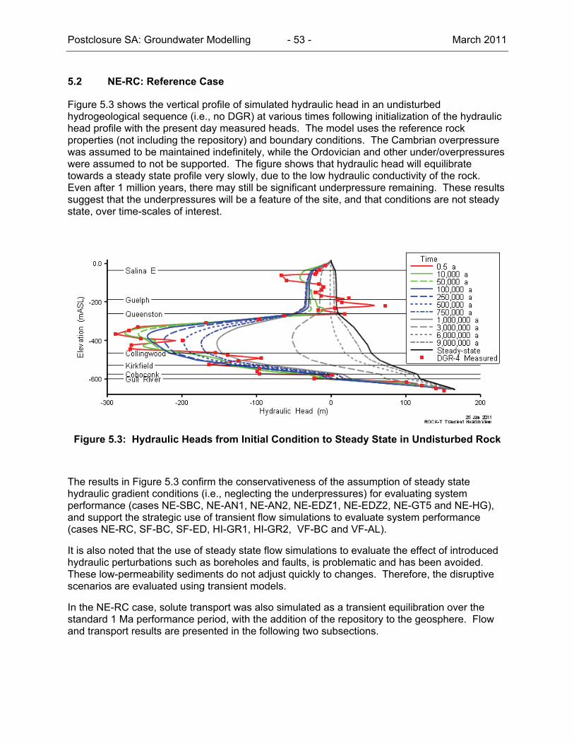
Postclosure SA: Groundwater Modelling - 53 - March 2011
5.2 NE-RC: Reference Case
Figure 5.3 shows the vertical profile of simulated hydraulic head in an undisturbed hydrogeological sequence (i.e., no DGR) at various times following initialization of the hydraulic head profile with the present day measured heads. The model uses the reference rock properties (not including the repository) and boundary conditions. The Cambrian overpressure was assumed to be maintained indefinitely, while the Ordovician and other under/overpressures were assumed to not be supported. The figure shows that hydraulic head will equilibrate towards a steady state profile very slowly, due to the low hydraulic conductivity of the rock. Even after 1 million years, there may still be significant underpressure remaining. These results suggest that the underpressures will be a feature of the site, and that conditions are not steady state, over time-scales of interest.
Figure 5.3: Hydraulic Heads from Initial Condition to Steady State in Undisturbed Rock
The results in Figure 5.3 confirm the conservativeness of the assumption of steady state hydraulic gradient conditions (i.e., neglecting the underpressures) for evaluating system performance (cases NE-SBC, NE-AN1, NE-AN2, NE-EDZ1, NE-EDZ2, NE-GT5 and NE-HG), and support the strategic use of transient flow simulations to evaluate system performance (cases NE-RC, SF-BC, SF-ED, HI-GR1, HI-GR2, VF-BC and VF-AL).
It is also noted that the use of steady state flow simulations to evaluate the effect of introduced hydraulic perturbations such as boreholes and faults, is problematic and has been avoided. These low-permeability sediments do not adjust quickly to changes. Therefore, the disruptive scenarios are evaluated using transient models.
In the NE-RC case, solute transport was also simulated as a transient equilibration over the standard 1 Ma performance period, with the addition of the repository to the geosphere. Flow and transport results are presented in the following two subsections.
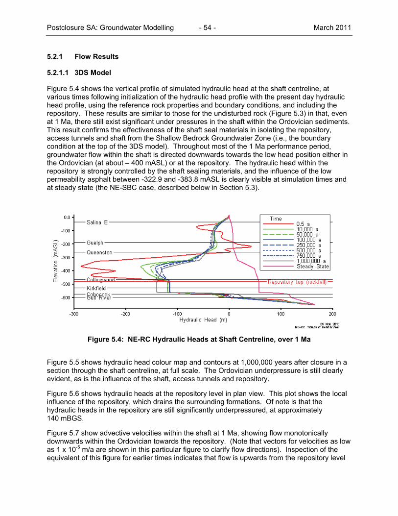
Postclosure SA: Groundwater Modelling - 54 - March 2011
5.2.1 Flow Results
5.2.1.1 3DS Model
Figure 5.4 shows the vertical profile of simulated hydraulic head at the shaft centreline, at various times following initialization of the hydraulic head profile with the present day hydraulic head profile, using the reference rock properties and boundary conditions, and including the repository. These results are similar to those for the undisturbed rock (Figure 5.3) in that, even at 1 Ma, there still exist significant under pressures in the shaft within the Ordovician sediments. This result confirms the effectiveness of the shaft seal materials in isolating the repository, access tunnels and shaft from the Shallow Bedrock Groundwater Zone (i.e., the boundary condition at the top of the 3DS model). Throughout most of the 1 Ma performance period, groundwater flow within the shaft is directed downwards towards the low head position either in the Ordovician (at about – 400 mASL) or at the repository. The hydraulic head within the repository is strongly controlled by the shaft sealing materials, and the influence of the low permeability asphalt between -322.9 and -383.8 mASL is clearly visible at simulation times and at steady state (the NE-SBC case, described below in Section 5.3).
Figure 5.4: NE-RC Hydraulic Heads at Shaft Centreline, over 1 Ma
Figure 5.5 shows hydraulic head colour map and contours at 1,000,000 years after closure in a section through the shaft centreline, at full scale. The Ordovician underpressure is still clearly evident, as is the influence of the shaft, access tunnels and repository.
Figure 5.6 shows hydraulic heads at the repository level in plan view. This plot shows the local influence of the repository, which drains the surrounding formations. Of note is that the hydraulic heads in the repository are still significantly underpressured, at approximately 140 mBGS.
Figure 5.7 show advective velocities within the shaft at 1 Ma, showing flow monotonically downwards within the Ordovician towards the repository. (Note that vectors for velocities as low as 1 x 10⁻⁵ m/a are shown in this particular figure to clarify flow directions). Inspection of the equivalent of this figure for earlier times indicates that flow is upwards from the repository level
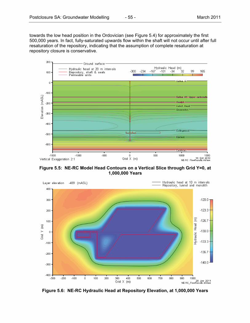
Postclosure SA: Groundwater Modelling - 55 - March 2011
towards the low head position in the Ordovician (see Figure 5.4) for approximately the first 500,000 years. In fact, fully-saturated upwards flow within the shaft will not occur until after full resaturation of the repository, indicating that the assumption of complete resaturation at repository closure is conservative.
Figure 5.5: NE-RC Model Head Contours on a Vertical Slice through Grid Y=0, at 1,000,000 Years
Figure 5.6: NE-RC Hydraulic Head at Repository Elevation, at 1,000,000 Years
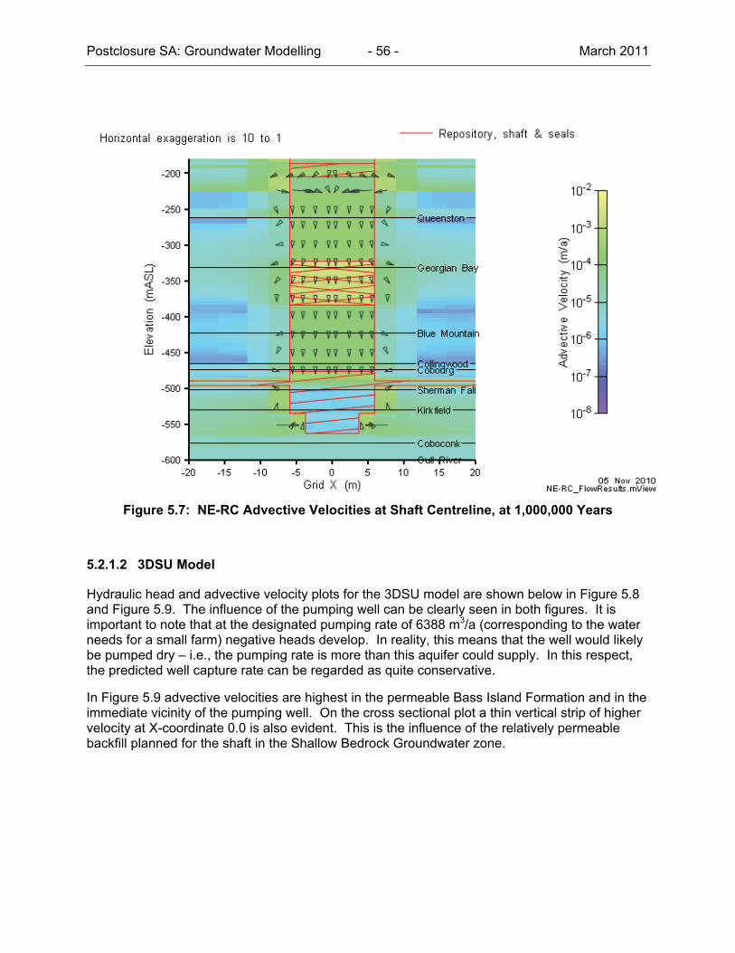
Postclosure SA: Groundwater Modelling - 56 - March 2011
Figure 5.7: NE-RC Advective Velocities at Shaft Centreline, at 1,000,000 Years
5.2.1.2 3DSU Model
Hydraulic head and advective velocity plots for the 3DSU model are shown below in Figure 5.8 and Figure 5.9. The influence of the pumping well can be clearly seen in both figures. It is important to note that at the designated pumping rate of 6388 m3/a (corresponding to the water needs for a small farm) negative heads develop. In reality, this means that the well would likely be pumped dry – i.e., the pumping rate is more than this aquifer could supply. In this respect, the predicted well capture rate can be regarded as quite conservative.
In Figure 5.9 advective velocities are highest in the permeable Bass Island Formation and in the immediate vicinity of the pumping well. On the cross sectional plot a thin vertical strip of higher velocity at X-coordinate 0.0 is also evident. This is the influence of the relatively permeable backfill planned for the shaft in the Shallow Bedrock Groundwater zone.

Postclosure SA: Groundwater Modelling - 57 - March 2011
Figure 5.8: NE-RC-3DSU Head Contours
Figure 5.9: NE-RC-3DSU Advective Velocity Magnitude and Vectors
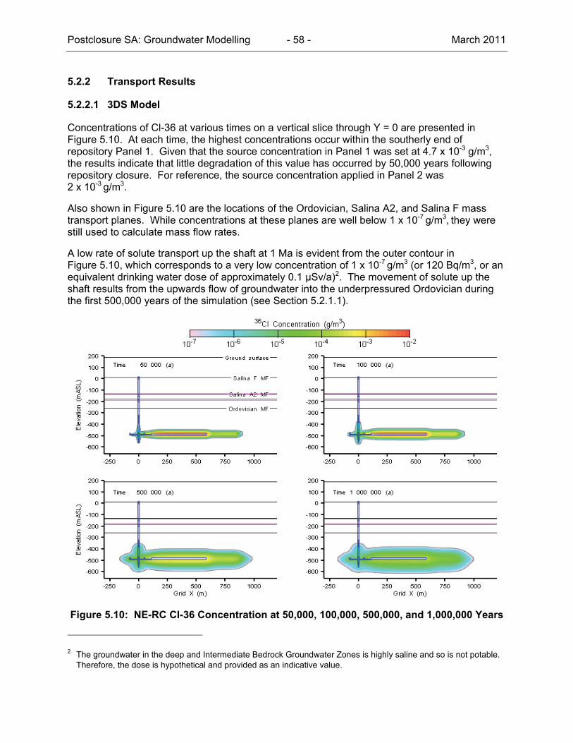
Postclosure SA: Groundwater Modelling - 58 - March 2011
5.2.2 Transport Results
5.2.2.1 3DS Model
Concentrations of Cl-36 at various times on a vertical slice through Y = 0 are presented in Figure 5.10. At each time, the highest concentrations occur within the southerly end of repository Panel 1. Given that the source concentration in Panel 1 was set at 4.7 x 10⁻³ g/m3, the results indicate that little degradation of this value has occurred by 50,000 years following repository closure. For reference, the source concentration applied in Panel 2 was 2 x 10⁻³ g/m3.
Also shown in Figure 5.10 are the locations of the Ordovician, Salina A2, and Salina F mass transport planes. While concentrations at these planes are well below 1 x 10⁻⁷ g/m3, they were still used to calculate mass flow rates.
A low rate of solute transport up the shaft at 1 Ma is evident from the outer contour in Figure 5.10, which corresponds to a very low concentration of 1 x 10⁻⁷ g/m3 (or 120 Bq/m3, or an equivalent drinking water dose of approximately 0.1 μSv/a)2. The movement of solute up the shaft results from the upwards flow of groundwater into the underpressured Ordovician during the first 500,000 years of the simulation (see Section 5.2.1.1).
Figure 5.10: NE-RC Cl-36 Concentration at 50,000, 100,000, 500,000, and 1,000,000 Years
2 The groundwater in the deep and Intermediate Bedrock Groundwater Zones is highly saline and so is not potable. Therefore, the dose is hypothetical and provided as an indicative value.
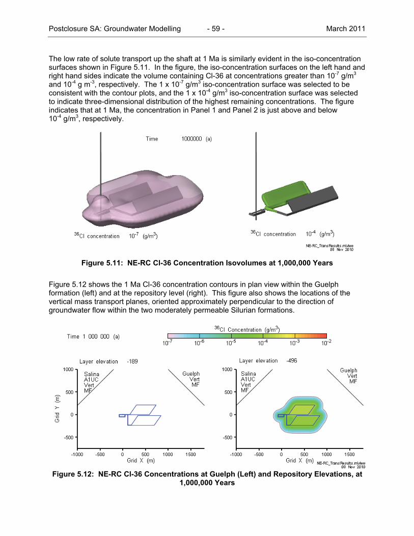
Postclosure SA: Groundwater Modelling - 59 - March 2011
The low rate of solute transport up the shaft at 1 Ma is similarly evident in the iso-concentration surfaces shown in Figure 5.11. In the figure, the iso-concentration surfaces on the left hand and right hand sides indicate the volume containing Cl-36 at concentrations greater than 10-7 g/m3 and 10-4 g m-3, respectively. The 1 x 10⁻⁷ g/m3 iso-concentration surface was selected to be consistent with the contour plots, and the 1 x 10⁻⁴ g/m3 iso-concentration surface was selected to indicate three-dimensional distribution of the highest remaining concentrations. The figure indicates that at 1 Ma, the concentration in Panel 1 and Panel 2 is just above and below 10-4 g/m3, respectively.
Figure 5.11: NE-RC Cl-36 Concentration Isovolumes at 1,000,000 Years
Figure 5.12 shows the 1 Ma Cl-36 concentration contours in plan view within the Guelph formation (left) and at the repository level (right). This figure also shows the locations of the vertical mass transport planes, oriented approximately perpendicular to the direction of groundwater flow within the two moderately permeable Silurian formations.
Figure 5.12: NE-RC Cl-36 Concentrations at Guelph (Left) and Repository Elevations, at
1,000,000 Years
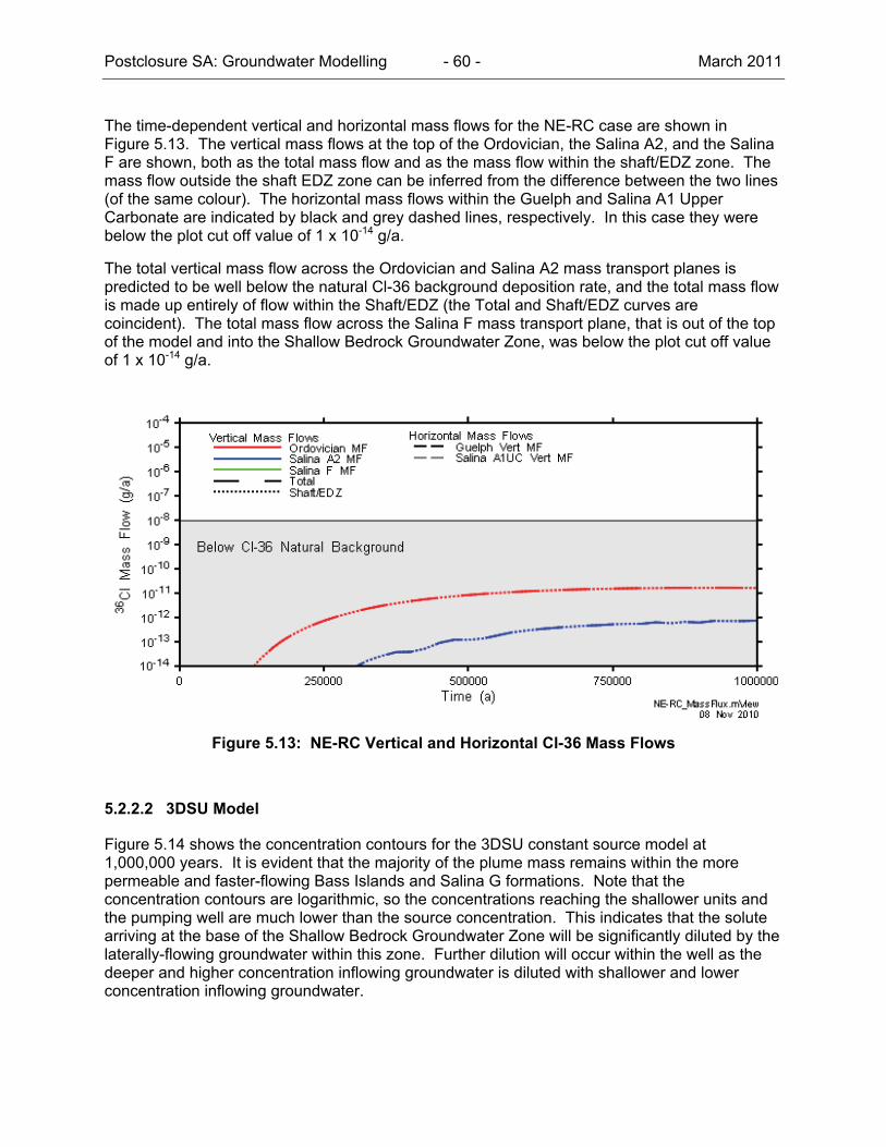
Postclosure SA: Groundwater Modelling - 60 - March 2011
The time-dependent vertical and horizontal mass flows for the NE-RC case are shown in Figure 5.13. The vertical mass flows at the top of the Ordovician, the Salina A2, and the Salina F are shown, both as the total mass flow and as the mass flow within the shaft/EDZ zone. The mass flow outside the shaft EDZ zone can be inferred from the difference between the two lines (of the same colour). The horizontal mass flows within the Guelph and Salina A1 Upper Carbonate are indicated by black and grey dashed lines, respectively. In this case they were below the plot cut off value of 1 x 10-14 g/a.
The total vertical mass flow across the Ordovician and Salina A2 mass transport planes is predicted to be well below the natural Cl-36 background deposition rate, and the total mass flow is made up entirely of flow within the Shaft/EDZ (the Total and Shaft/EDZ curves are coincident). The total mass flow across the Salina F mass transport plane, that is out of the top of the model and into the Shallow Bedrock Groundwater Zone, was below the plot cut off value of 1 x 10-14 g/a.
Figure 5.13: NE-RC Vertical and Horizontal Cl-36 Mass Flows
5.2.2.2 3DSU Model
Figure 5.14 shows the concentration contours for the 3DSU constant source model at 1,000,000 years. It is evident that the majority of the plume mass remains within the more permeable and faster-flowing Bass Islands and Salina G formations. Note that the concentration contours are logarithmic, so the concentrations reaching the shallower units and the pumping well are much lower than the source concentration. This indicates that the solute arriving at the base of the Shallow Bedrock Groundwater Zone will be significantly diluted by the laterally-flowing groundwater within this zone. Further dilution will occur within the well as the deeper and higher concentration inflowing groundwater is diluted with shallower and lower concentration inflowing groundwater.
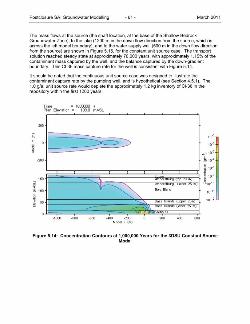
Postclosure SA: Groundwater Modelling - 61 - March 2011
The mass flows at the source (the shaft location, at the base of the Shallow Bedrock Groundwater Zone), to the lake (1200 m in the down flow direction from the source, which is across the left model boundary), and to the water supply well (500 m in the down flow direction from the source) are shown in Figure 5.15, for the constant unit source case. The transport solution reached steady state at approximately 70,000 years, with approximately 1.15% of the contaminant mass captured by the well, and the balance captured by the down-gradient boundary. This Cl-36 mass capture rate for the well is consistent with Figure 5.14.
It should be noted that the continuous unit source case was designed to illustrate the contaminant capture rate by the pumping well, and is hypothetical (see Section 4.5.1). The 1.0 g/a, unit source rate would deplete the approximately 1.2 kg inventory of Cl-36 in the repository within the first 1200 years.
Figure 5.14: Concentration Contours at 1,000,000 Years for the 3DSU Constant Source Model
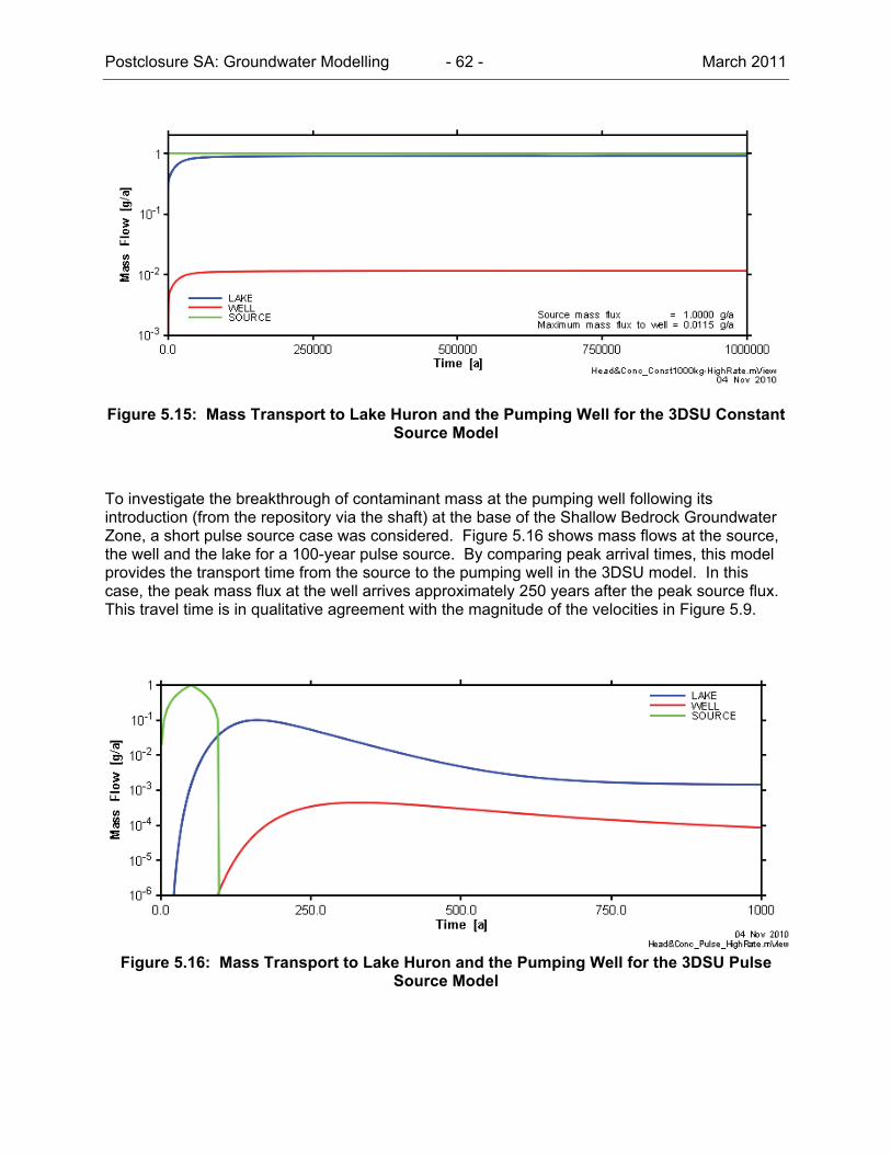
Postclosure SA: Groundwater Modelling - 62 - March 2011
Figure 5.15: Mass Transport to Lake Huron and the Pumping Well for the 3DSU Constant Source Model
To investigate the breakthrough of contaminant mass at the pumping well following its introduction (from the repository via the shaft) at the base of the Shallow Bedrock Groundwater Zone, a short pulse source case was considered. Figure 5.16 shows mass flows at the source, the well and the lake for a 100-year pulse source. By comparing peak arrival times, this model provides the transport time from the source to the pumping well in the 3DSU model. In this case, the peak mass flux at the well arrives approximately 250 years after the peak source flux. This travel time is in qualitative agreement with the magnitude of the velocities in Figure 5.9.
Figure 5.16: Mass Transport to Lake Huron and the Pumping Well for the 3DSU Pulse
Source Model
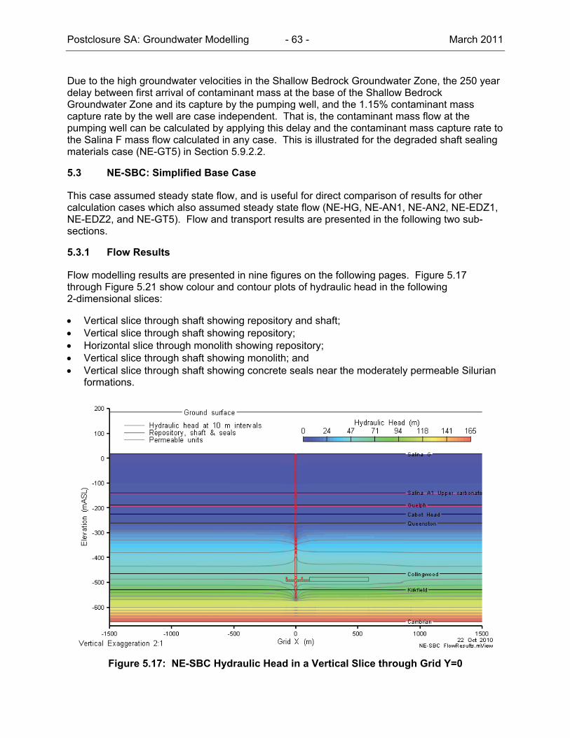
Postclosure SA: Groundwater Modelling - 63 - March 2011
Due to the high groundwater velocities in the Shallow Bedrock Groundwater Zone, the 250 year delay between first arrival of contaminant mass at the base of the Shallow Bedrock Groundwater Zone and its capture by the pumping well, and the 1.15% contaminant mass capture rate by the well are case independent. That is, the contaminant mass flow at the pumping well can be calculated by applying this delay and the contaminant mass capture rate to the Salina F mass flow calculated in any case. This is illustrated for the degraded shaft sealing materials case (NE-GT5) in Section 5.9.2.2.
5.3 NE-SBC: Simplified Base Case
This case assumed steady state flow, and is useful for direct comparison of results for other calculation cases which also assumed steady state flow (NE-HG, NE-AN1, NE-AN2, NE-EDZ1, NE-EDZ2, and NE-GT5). Flow and transport results are presented in the following two sub-sections.
5.3.1 Flow Results
Flow modelling results are presented in nine figures on the following pages. Figure 5.17 through Figure 5.21 show colour and contour plots of hydraulic head in the following 2-dimensional slices:
Vertical slice through shaft showing repository and shaft; Vertical slice through shaft showing repository; Horizontal slice through monolith showing repository; Vertical slice through shaft showing monolith; and Vertical slice through shaft showing concrete seals near the moderately permeable Silurian
formations.
Figure 5.17: NE-SBC Hydraulic Head in a Vertical Slice through Grid Y=0
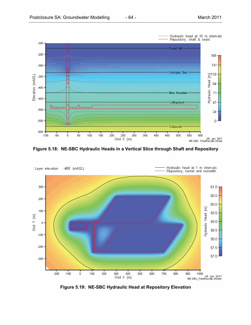
Postclosure SA: Groundwater Modelling - 64 - March 2011
Figure 5.18: NE-SBC Hydraulic Heads in a Vertical Slice through Shaft and Repository
Figure 5.19: NE-SBC Hydraulic Head at Repository Elevation
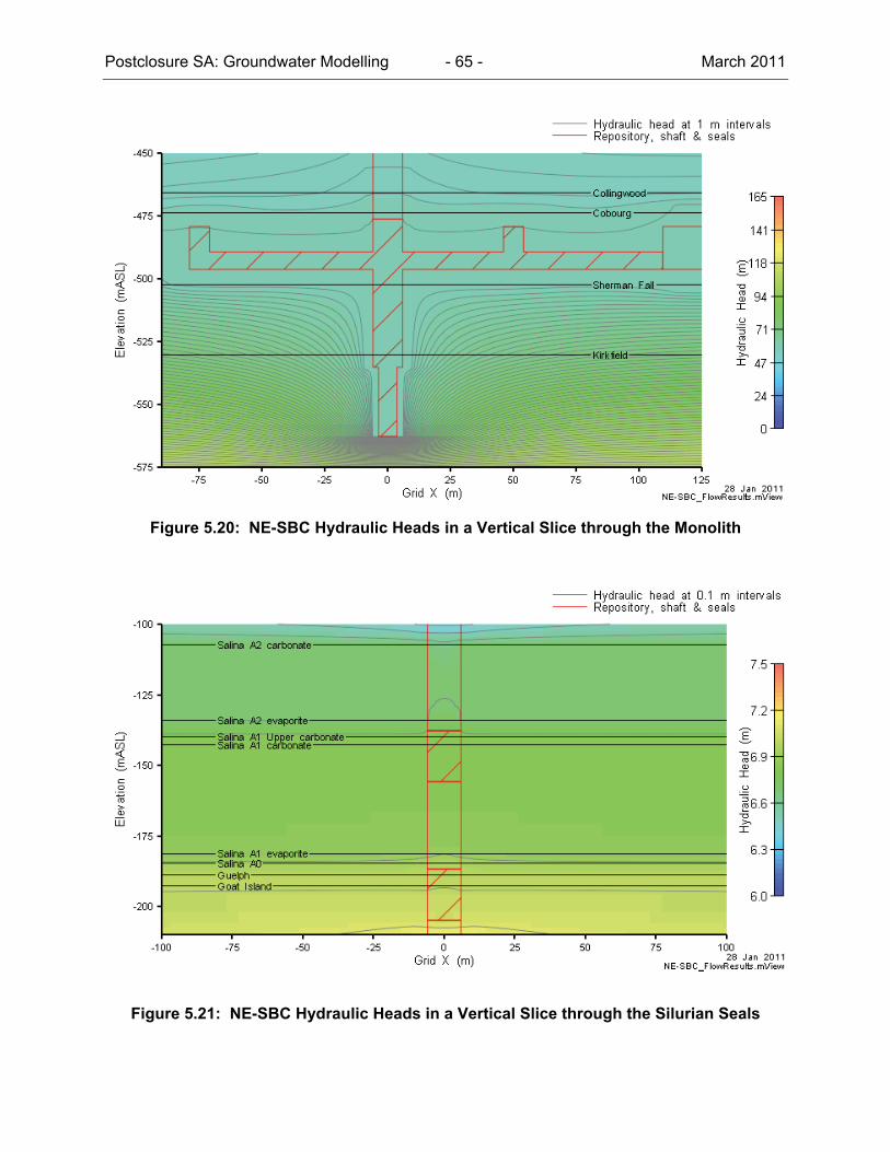
Postclosure SA: Groundwater Modelling - 65 - March 2011
Figure 5.20: NE-SBC Hydraulic Heads in a Vertical Slice through the Monolith
Figure 5.21: NE-SBC Hydraulic Heads in a Vertical Slice through the Silurian Seals

Postclosure SA: Groundwater Modelling - 66 - March 2011
The hydraulic heads in Figure 5.17 through Figure 5.21 indicate the steady state head distribution, with the repository as designed. The hydraulic head distribution is strongly controlled by the hydraulic conductivity of the host rock formations, and the majority of the head variation (drop) is observed across the formations with the lowest vertical hydraulic conductivity, being the Gull River and Kirkfield formations below the repository. The relatively small perturbation of the hydraulic head caused by the presence of the repository and shaft (there is only a few metres difference between the hydraulic head in the repository and the ambient hydraulic head at repository depth in Figure 5.19, and in Figure 5.17) indicates that the shaft sealing system is effective in isolating the repository from the surface, and the head in the repository, at approximately 57 m above ground surface (mAGS), appears to be most strongly controlled by the host rock hydraulic conductivities. At 1 Ma in the NE-RC case, the hydraulic head in the repository was still significantly underpressured (124 mBGS), and the results of the transient simulations indicate that this switch from under to over pressured repository may take several million years to occur. This serves to remind the reader that the steady state flow condition in this Simplified Base Case model is a conservative assumption.
Figure 5.22 through Figure 5.26 show the advective velocity magnitudes and vectors on the same 2-dimensional slices as illustrated in Figure 5.17 through Figure 5.21, respectively.
Figure 5.22: NE-SBC Advective Velocity Magnitude and Vectors on a Vertical Slice through Grid Y=0
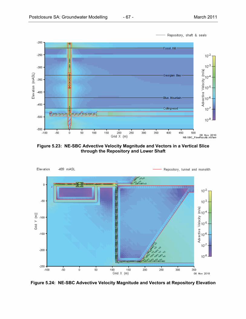
Postclosure SA: Groundwater Modelling - 67 - March 2011
Figure 5.23: NE-SBC Advective Velocity Magnitude and Vectors in a Vertical Slice through the Repository and Lower Shaft
Figure 5.24: NE-SBC Advective Velocity Magnitude and Vectors at Repository Elevation
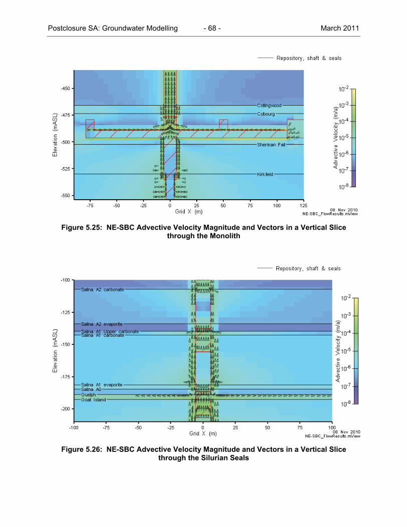
Postclosure SA: Groundwater Modelling - 68 - March 2011
Figure 5.25: NE-SBC Advective Velocity Magnitude and Vectors in a Vertical Slice through the Monolith
Figure 5.26: NE-SBC Advective Velocity Magnitude and Vectors in a Vertical Slice through the Silurian Seals
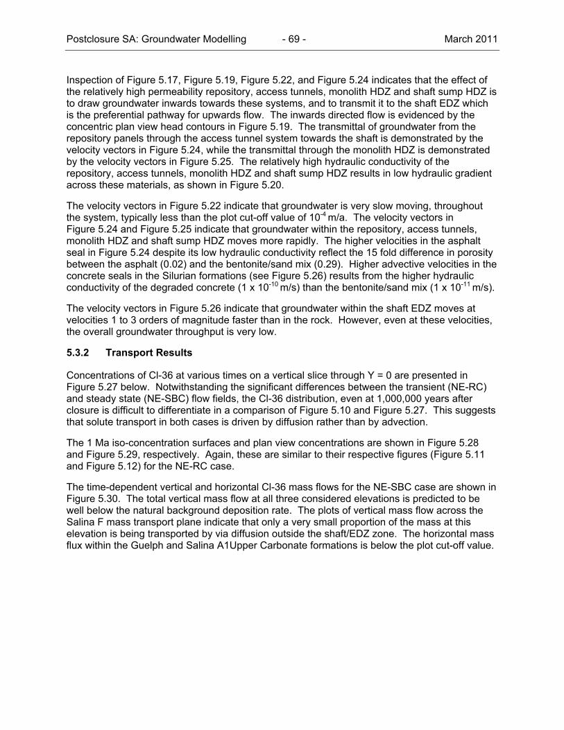
Postclosure SA: Groundwater Modelling - 69 - March 2011
Inspection of Figure 5.17, Figure 5.19, Figure 5.22, and Figure 5.24 indicates that the effect of the relatively high permeability repository, access tunnels, monolith HDZ and shaft sump HDZ is to draw groundwater inwards towards these systems, and to transmit it to the shaft EDZ which is the preferential pathway for upwards flow. The inwards directed flow is evidenced by the concentric plan view head contours in Figure 5.19. The transmittal of groundwater from the repository panels through the access tunnel system towards the shaft is demonstrated by the velocity vectors in Figure 5.24, while the transmittal through the monolith HDZ is demonstrated by the velocity vectors in Figure 5.25. The relatively high hydraulic conductivity of the repository, access tunnels, monolith HDZ and shaft sump HDZ results in low hydraulic gradient across these materials, as shown in Figure 5.20.
The velocity vectors in Figure 5.22 indicate that groundwater is very slow moving, throughout the system, typically less than the plot cut-off value of 10-4 m/a. The velocity vectors in Figure 5.24 and Figure 5.25 indicate that groundwater within the repository, access tunnels, monolith HDZ and shaft sump HDZ moves more rapidly. The higher velocities in the asphalt seal in Figure 5.24 despite its low hydraulic conductivity reflect the 15 fold difference in porosity between the asphalt (0.02) and the bentonite/sand mix (0.29). Higher advective velocities in the concrete seals in the Silurian formations (see Figure 5.26) results from the higher hydraulic conductivity of the degraded concrete (1 x 10⁻¹⁰ m/s) than the bentonite/sand mix (1 x 10-11 m/s).
The velocity vectors in Figure 5.26 indicate that groundwater within the shaft EDZ moves at velocities 1 to 3 orders of magnitude faster than in the rock. However, even at these velocities, the overall groundwater throughput is very low.
5.3.2 Transport Results
Concentrations of Cl-36 at various times on a vertical slice through Y = 0 are presented in Figure 5.27 below. Notwithstanding the significant differences between the transient (NE-RC) and steady state (NE-SBC) flow fields, the Cl-36 distribution, even at 1,000,000 years after closure is difficult to differentiate in a comparison of Figure 5.10 and Figure 5.27. This suggests that solute transport in both cases is driven by diffusion rather than by advection.
The 1 Ma iso-concentration surfaces and plan view concentrations are shown in Figure 5.28 and Figure 5.29, respectively. Again, these are similar to their respective figures (Figure 5.11 and Figure 5.12) for the NE-RC case.
The time-dependent vertical and horizontal Cl-36 mass flows for the NE-SBC case are shown in Figure 5.30. The total vertical mass flow at all three considered elevations is predicted to be well below the natural background deposition rate. The plots of vertical mass flow across the Salina F mass transport plane indicate that only a very small proportion of the mass at this elevation is being transported by via diffusion outside the shaft/EDZ zone. The horizontal mass flux within the Guelph and Salina A1Upper Carbonate formations is below the plot cut-off value.

Postclosure SA: Groundwater Modelling - 70 - March 2011
Figure 5.27: NE-SBC Cl-36 Concentration at 50,000, 100,000, 500,000, and 1,000,000 Years
Figure 5.28: NE-SBC Cl-36 Concentration Isovolumes at 1,000,000 Years
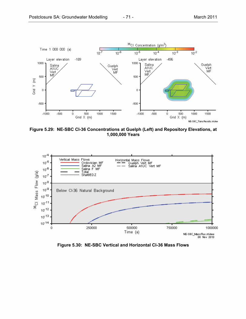
Postclosure SA: Groundwater Modelling - 71 - March 2011
Figure 5.29: NE-SBC Cl-36 Concentrations at Guelph (Left) and Repository Elevations, at 1,000,000 Years
Figure 5.30: NE-SBC Vertical and Horizontal Cl-36 Mass Flows
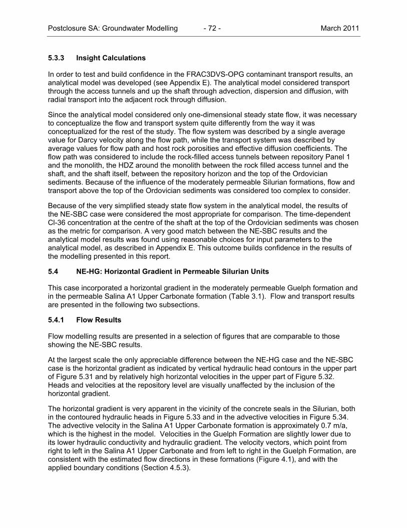
Postclosure SA: Groundwater Modelling - 72 - March 2011
5.3.3 Insight Calculations
In order to test and build confidence in the FRAC3DVS-OPG contaminant transport results, an analytical model was developed (see Appendix E). The analytical model considered transport through the access tunnels and up the shaft through advection, dispersion and diffusion, with radial transport into the adjacent rock through diffusion.
Since the analytical model considered only one-dimensional steady state flow, it was necessary to conceptualize the flow and transport system quite differently from the way it was conceptualized for the rest of the study. The flow system was described by a single average value for Darcy velocity along the flow path, while the transport system was described by average values for flow path and host rock porosities and effective diffusion coefficients. The flow path was considered to include the rock-filled access tunnels between repository Panel 1 and the monolith, the HDZ around the monolith between the rock filled access tunnel and the shaft, and the shaft itself, between the repository horizon and the top of the Ordovician sediments. Because of the influence of the moderately permeable Silurian formations, flow and transport above the top of the Ordovician sediments was considered too complex to consider.
Because of the very simplified steady state flow system in the analytical model, the results of the NE-SBC case were considered the most appropriate for comparison. The time-dependent Cl-36 concentration at the centre of the shaft at the top of the Ordovician sediments was chosen as the metric for comparison. A very good match between the NE-SBC results and the analytical model results was found using reasonable choices for input parameters to the analytical model, as described in Appendix E. This outcome builds confidence in the results of the modelling presented in this report.
5.4 NE-HG: Horizontal Gradient in Permeable Silurian Units
This case incorporated a horizontal gradient in the moderately permeable Guelph formation and in the permeable Salina A1 Upper Carbonate formation (Table 3.1). Flow and transport results are presented in the following two subsections.
5.4.1 Flow Results
Flow modelling results are presented in a selection of figures that are comparable to those showing the NE-SBC results.
At the largest scale the only appreciable difference between the NE-HG case and the NE-SBC case is the horizontal gradient as indicated by vertical hydraulic head contours in the upper part of Figure 5.31 and by relatively high horizontal velocities in the upper part of Figure 5.32. Heads and velocities at the repository level are visually unaffected by the inclusion of the horizontal gradient.
The horizontal gradient is very apparent in the vicinity of the concrete seals in the Silurian, both in the contoured hydraulic heads in Figure 5.33 and in the advective velocities in Figure 5.34. The advective velocity in the Salina A1 Upper Carbonate formation is approximately 0.7 m/a, which is the highest in the model. Velocities in the Guelph Formation are slightly lower due to its lower hydraulic conductivity and hydraulic gradient. The velocity vectors, which point from right to left in the Salina A1 Upper Carbonate and from left to right in the Guelph Formation, are consistent with the estimated flow directions in these formations (Figure 4.1), and with the applied boundary conditions (Section 4.5.3).
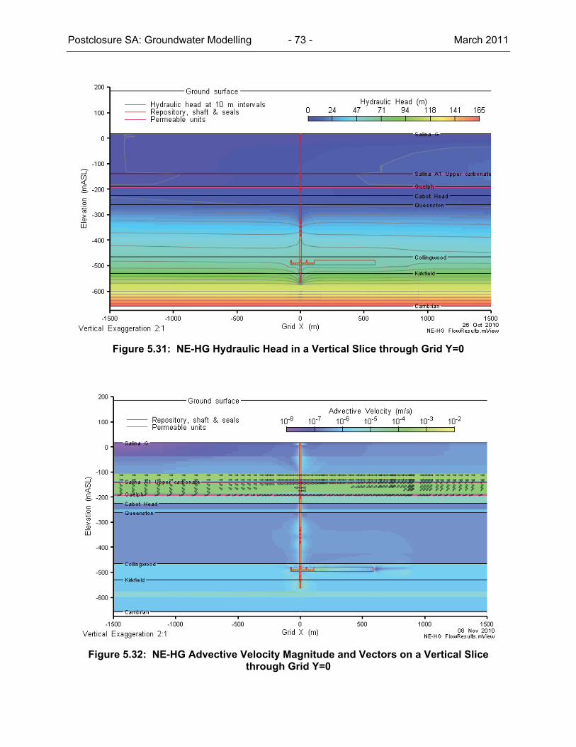
Postclosure SA: Groundwater Modelling - 73 - March 2011
Figure 5.31: NE-HG Hydraulic Head in a Vertical Slice through Grid Y=0
Figure 5.32: NE-HG Advective Velocity Magnitude and Vectors on a Vertical Slice through Grid Y=0

Postclosure SA: Groundwater Modelling - 74 - March 2011
Figure 5.33: NE-HG Hydraulic Heads in a Vertical Slice through the Silurian Seals
Figure 5.34: NE-HG Advective Velocity Magnitude and Vectors in a Vertical Slice through the Silurian Seals
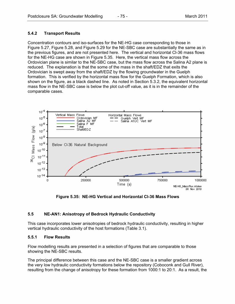
Postclosure SA: Groundwater Modelling - 75 - March 2011
5.4.2 Transport Results
Concentration contours and iso-surfaces for the NE-HG case corresponding to those in Figure 5.27, Figure 5.28, and Figure 5.29 for the NE-SBC case are substantially the same as in the previous figures, and are not presented here. The vertical and horizontal Cl-36 mass flows for the NE-HG case are shown in Figure 5.35. Here, the vertical mass flow across the Ordovician plane is similar to the NE-SBC case, but the mass flow across the Salina A2 plane is reduced. The explanation is that the some of the mass in the shaft/EDZ that exits the Ordovician is swept away from the shaft/EDZ by the flowing groundwater in the Guelph formation. This is verified by the horizontal mass flow for the Guelph Formation, which is also shown on the figure, as a black dashed line. As noted in Section 5.3.2, the equivalent horizontal mass flow in the NE-SBC case is below the plot cut-off value, as it is in the remainder of the comparable cases.
Figure 5.35: NE-HG Vertical and Horizontal Cl-36 Mass Flows
5.5 NE-AN1: Anisotropy of Bedrock Hydraulic Conductivity
This case incorporates lower anisotropies of bedrock hydraulic conductivity, resulting in higher vertical hydraulic conductivity of the host formations (Table 3.1).
5.5.1 Flow Results
Flow modelling results are presented in a selection of figures that are comparable to those showing the NE-SBC results.
The principal difference between this case and the NE-SBC case is a smaller gradient across the very low hydraulic conductivity formations below the repository (Coboconk and Gull River), resulting from the change of anisotropy for these formation from 1000:1 to 20:1. As a result, the
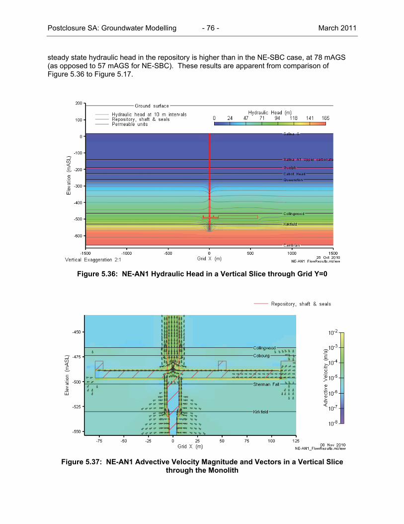
Postclosure SA: Groundwater Modelling - 76 - March 2011
steady state hydraulic head in the repository is higher than in the NE-SBC case, at 78 mAGS (as opposed to 57 mAGS for NE-SBC). These results are apparent from comparison of Figure 5.36 to Figure 5.17.
Figure 5.36: NE-AN1 Hydraulic Head in a Vertical Slice through Grid Y=0
Figure 5.37: NE-AN1 Advective Velocity Magnitude and Vectors in a Vertical Slice through the Monolith
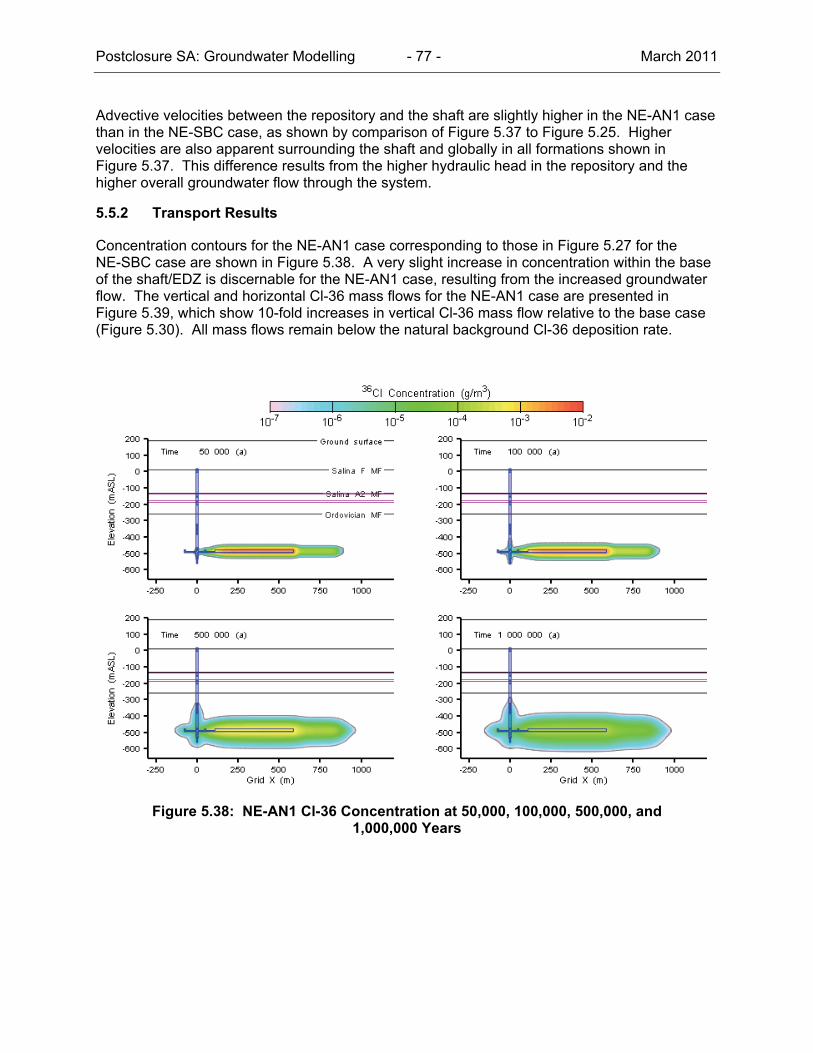
Postclosure SA: Groundwater Modelling - 77 - March 2011
Advective velocities between the repository and the shaft are slightly higher in the NE-AN1 case than in the NE-SBC case, as shown by comparison of Figure 5.37 to Figure 5.25. Higher velocities are also apparent surrounding the shaft and globally in all formations shown in Figure 5.37. This difference results from the higher hydraulic head in the repository and the higher overall groundwater flow through the system.
5.5.2 Transport Results
Concentration contours for the NE-AN1 case corresponding to those in Figure 5.27 for the NE-SBC case are shown in Figure 5.38. A very slight increase in concentration within the base of the shaft/EDZ is discernable for the NE-AN1 case, resulting from the increased groundwater flow. The vertical and horizontal Cl-36 mass flows for the NE-AN1 case are presented in Figure 5.39, which show 10-fold increases in vertical Cl-36 mass flow relative to the base case (Figure 5.30). All mass flows remain below the natural background Cl-36 deposition rate.
Figure 5.38: NE-AN1 Cl-36 Concentration at 50,000, 100,000, 500,000, and 1,000,000 Years

Postclosure SA: Groundwater Modelling - 78 - March 2011
Figure 5.39: NE-AN1 Vertical and Horizontal Cl-36 Mass Flows
5.6 NE-AN2: Anisotropy of Bedrock Effective Diffusion Coefficients
This case incorporated higher horizontal effective diffusion coefficients relative to the NE-SBC case (Table 3.1). Flow results are not presented as the flow model is identical to NE-SBC.
5.6.1 Transport Results
Concentration contours for the NE-AN2 case corresponding to those in Figure 5.27 for the NE-SBC case are shown in Figure 5.40. Relative to the NE-SBC case, the Cl-36 plume is wider at the repository, resulting from the enhanced horizontal diffusion. The take up of mass by the rock has resulted in less mass travelling up the shaft/EDZ, and the total vertical Cl-36 mass flow is reduced relative to the NE-SBC case (Figure 5.30), as shown in Figure 5.41.
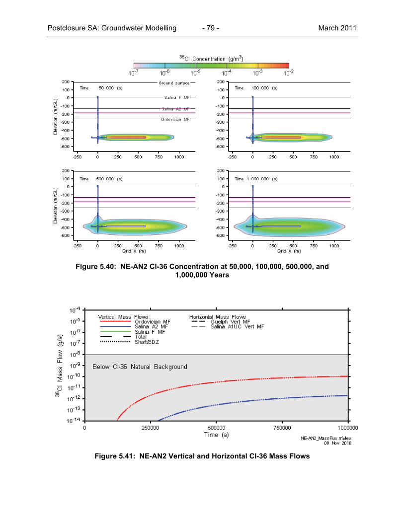
Postclosure SA: Groundwater Modelling - 79 - March 2011
Figure 5.40: NE-AN2 Cl-36 Concentration at 50,000, 100,000, 500,000, and 1,000,000 Years
Figure 5.41: NE-AN2 Vertical and Horizontal Cl-36 Mass Flows
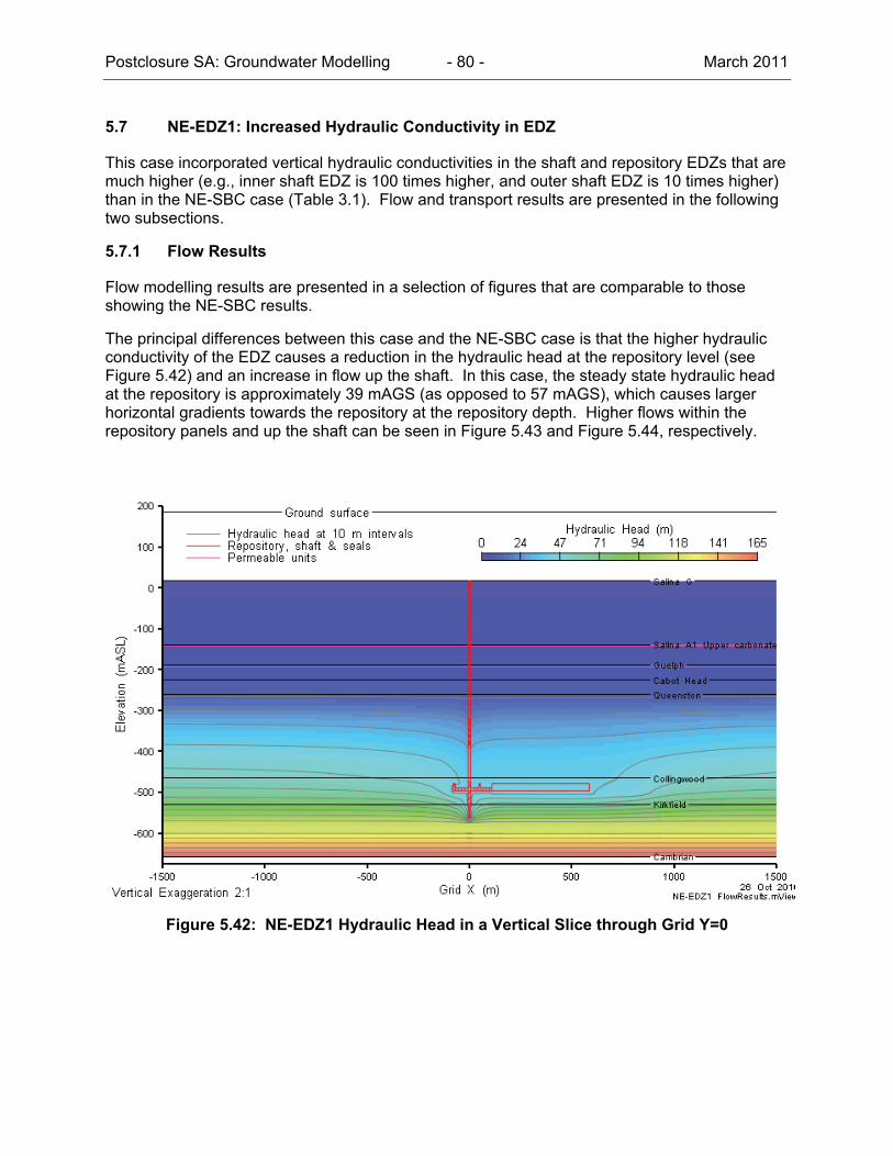
Postclosure SA: Groundwater Modelling - 80 - March 2011
5.7 NE-EDZ1: Increased Hydraulic Conductivity in EDZ
This case incorporated vertical hydraulic conductivities in the shaft and repository EDZs that are much higher (e.g., inner shaft EDZ is 100 times higher, and outer shaft EDZ is 10 times higher) than in the NE-SBC case (Table 3.1). Flow and transport results are presented in the following two subsections.
5.7.1 Flow Results
Flow modelling results are presented in a selection of figures that are comparable to those showing the NE-SBC results.
The principal differences between this case and the NE-SBC case is that the higher hydraulic conductivity of the EDZ causes a reduction in the hydraulic head at the repository level (see Figure 5.42) and an increase in flow up the shaft. In this case, the steady state hydraulic head at the repository is approximately 39 mAGS (as opposed to 57 mAGS), which causes larger horizontal gradients towards the repository at the repository depth. Higher flows within the repository panels and up the shaft can be seen in Figure 5.43 and Figure 5.44, respectively.
Figure 5.42: NE-EDZ1 Hydraulic Head in a Vertical Slice through Grid Y=0
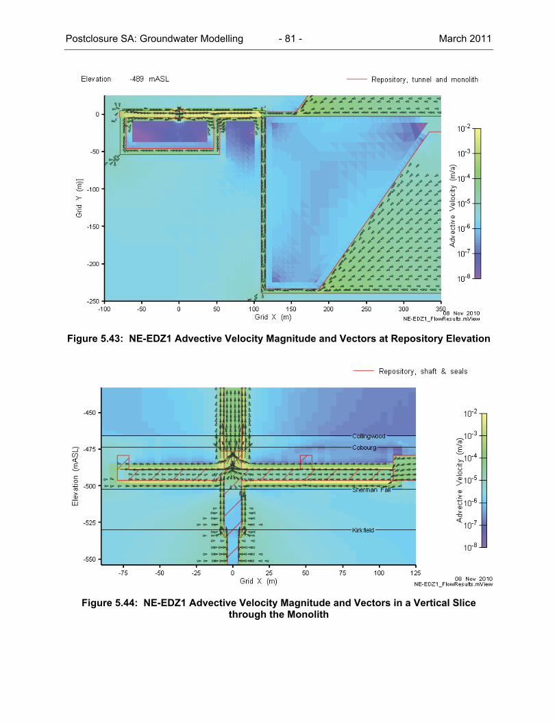
Postclosure SA: Groundwater Modelling - 81 - March 2011
Figure 5.43: NE-EDZ1 Advective Velocity Magnitude and Vectors at Repository Elevation
Figure 5.44: NE-EDZ1 Advective Velocity Magnitude and Vectors in a Vertical Slice through the Monolith

Postclosure SA: Groundwater Modelling - 82 - March 2011
Figure 5.45 shows advective velocities in plan view at the elevation of the HDZ immediately above the concrete monolith. This figure is included for comparison to results from the NE-EDZ2 case in Section 5.8.1.
Figure 5.45: NE-EDZ1 Advective Velocities at Keyed-in Monolith, in Plan View at Elevation of Overlying HDZ
5.7.2 Transport Results
Concentrations of Cl-36 at various times on a vertical slice through Y = 0 are presented in Figure 5.46. The higher groundwater throughput has resulted in greater transport of mass up the shaft/EDZ relative to the NE-SBC case (Figure 5.27), which is particularly apparent 500,000 years and 1,000,000 years after closure. Concentrations at the plotting limit of 10-7g/m3 have just reached the Salina A1 upper carbonate unit 500,000 years after closure. Solute transport up the shaft/EDZ at 1 Ma is similarly evident in the iso-concentration surfaces shown in Figure 5.47. Figure 5.48 indicates significantly higher total vertical Cl-36 mass flows than in the NE-SBC case, again entirely within the shaft/EDZ (inspection shows that most of the mass is actually being transported within the inner EDZ). However, the total mass flow into the Shallow Bedrock Groundwater Zone is still below the Cl-36 natural background deposition rate.
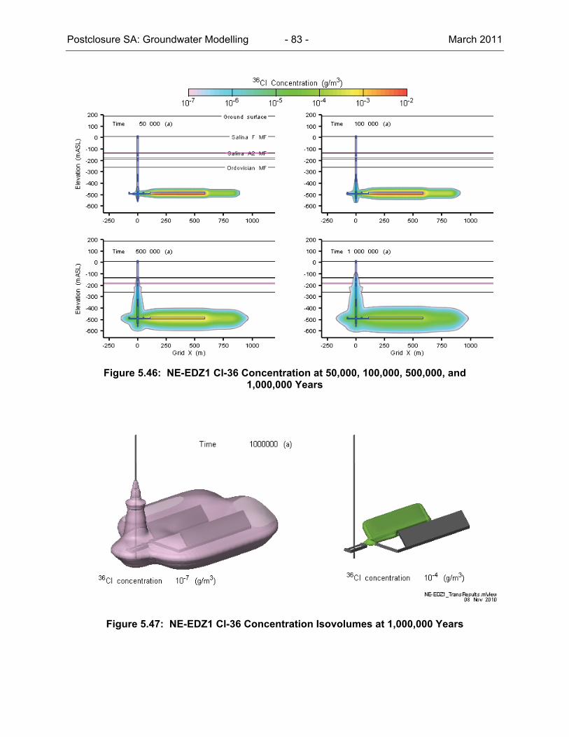
Postclosure SA: Groundwater Modelling - 83 - March 2011
Figure 5.46: NE-EDZ1 Cl-36 Concentration at 50,000, 100,000, 500,000, and 1,000,000 Years
Figure 5.47: NE-EDZ1 Cl-36 Concentration Isovolumes at 1,000,000 Years
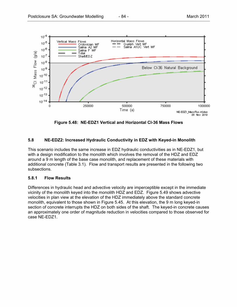
Postclosure SA: Groundwater Modelling - 84 - March 2011
Figure 5.48: NE-EDZ1 Vertical and Horizontal Cl-36 Mass Flows
5.8 NE-EDZ2: Increased Hydraulic Conductivity in EDZ with Keyed-in Monolith
This scenario includes the same increase in EDZ hydraulic conductivities as in NE-EDZ1, but with a design modification to the monolith which involves the removal of the HDZ and EDZ around a 9 m length of the base case monolith, and replacement of these materials with additional concrete (Table 3.1). Flow and transport results are presented in the following two subsections.
5.8.1 Flow Results
Differences in hydraulic head and advective velocity are imperceptible except in the immediate vicinity of the monolith keyed into the monolith HDZ and EDZ. Figure 5.49 shows advective velocities in plan view at the elevation of the HDZ immediately above the standard concrete monolith, equivalent to those shown in Figure 5.45. At this elevation, the 9 m long keyed-in section of concrete interrupts the HDZ on both sides of the shaft. The keyed-in concrete causes an approximately one order of magnitude reduction in velocities compared to those observed for case NE-EDZ1.

Postclosure SA: Groundwater Modelling - 85 - March 2011
Figure 5.49: NE-EDZ2 Advective Velocities at Keyed-in Monolith, in Plan View at Elevation of Overlying HDZ
5.8.2 Transport Results
Concentration contours and iso-surfaces for the NE-EDZ2 are substantially the same as those for NE-EDZ1 and are not included here. This indicates that the monolith modification was not effective in decreasing the mass transport of Cl-36 in this case, and relates to the high hydraulic conductivities of the EDZ, the relatively high hydraulic conductivity of the (assumed) degraded concrete, and the relatively short interruption of the flow path. Similarly, the Cl-36 mass flows for the NE-EDZ2 case are virtually identical to those for the NE-EDZ1 case shown in Figure 5.48.
5.9 NE-GT5: Increased Shaft Seal Hydraulic Conductivity
This case is equivalent to NE-SBC but with asphalt replaced by additional bentonite/sand, and the latter material having a 10 fold higher hydraulic conductivity than for NE-SBC. Flow and transport results are presented in the following two sub sections.
5.9.1 Flow Results
The hydraulic head distribution at the repository and the lower part of the shaft (including the asphalt seal zone) for this calculation case is shown in Figure 5.50. The effect of the modifications to the shaft seal materials is the elimination of the high hydraulic gradient across the asphalt seal (compare the equipotential lines in the double cross hatched area in Figure 5.50 to those in Figure 5.18), an overall reduction in hydraulic head at the repository
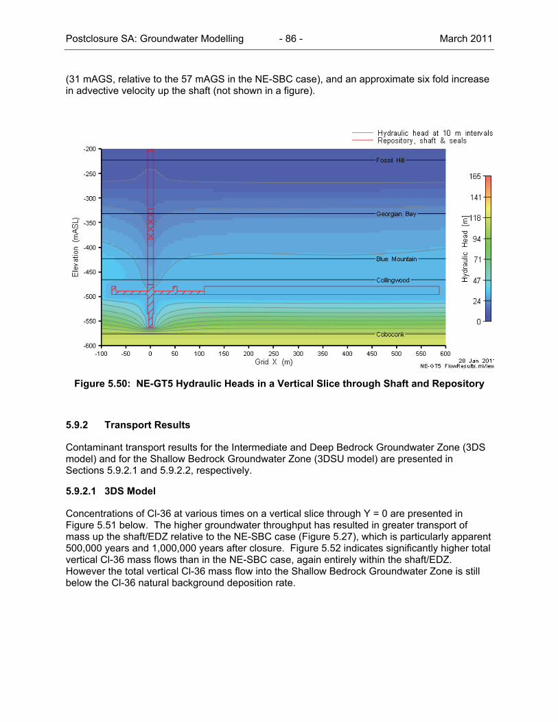
Postclosure SA: Groundwater Modelling - 86 - March 2011
(31 mAGS, relative to the 57 mAGS in the NE-SBC case), and an approximate six fold increase in advective velocity up the shaft (not shown in a figure).
Figure 5.50: NE-GT5 Hydraulic Heads in a Vertical Slice through Shaft and Repository
5.9.2 Transport Results
Contaminant transport results for the Intermediate and Deep Bedrock Groundwater Zone (3DS model) and for the Shallow Bedrock Groundwater Zone (3DSU model) are presented in Sections 5.9.2.1 and 5.9.2.2, respectively.
5.9.2.1 3DS Model
Concentrations of Cl-36 at various times on a vertical slice through Y = 0 are presented in Figure 5.51 below. The higher groundwater throughput has resulted in greater transport of mass up the shaft/EDZ relative to the NE-SBC case (Figure 5.27), which is particularly apparent 500,000 years and 1,000,000 years after closure. Figure 5.52 indicates significantly higher total vertical Cl-36 mass flows than in the NE-SBC case, again entirely within the shaft/EDZ. However the total vertical Cl-36 mass flow into the Shallow Bedrock Groundwater Zone is still below the Cl-36 natural background deposition rate.
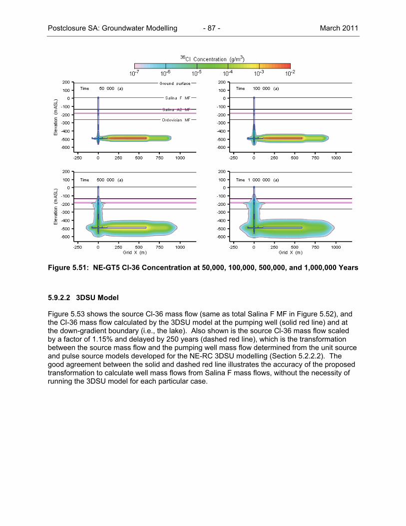
Postclosure SA: Groundwater Modelling - 87 - March 2011
Figure 5.51: NE-GT5 Cl-36 Concentration at 50,000, 100,000, 500,000, and 1,000,000 Years
5.9.2.2 3DSU Model
Figure 5.53 shows the source Cl-36 mass flow (same as total Salina F MF in Figure 5.52), and the Cl-36 mass flow calculated by the 3DSU model at the pumping well (solid red line) and at the down-gradient boundary (i.e., the lake). Also shown is the source Cl-36 mass flow scaled by a factor of 1.15% and delayed by 250 years (dashed red line), which is the transformation between the source mass flow and the pumping well mass flow determined from the unit source and pulse source models developed for the NE-RC 3DSU modelling (Section 5.2.2.2). The good agreement between the solid and dashed red line illustrates the accuracy of the proposed transformation to calculate well mass flows from Salina F mass flows, without the necessity of running the 3DSU model for each particular case.
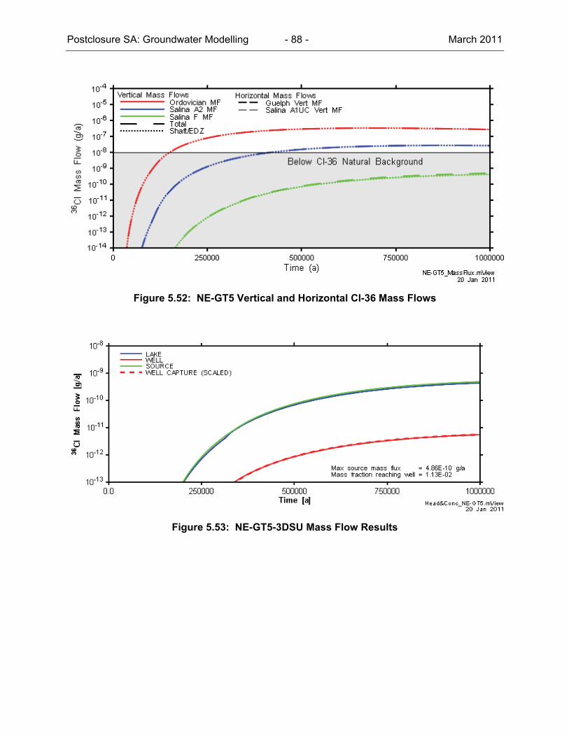
Postclosure SA: Groundwater Modelling - 88 - March 2011
Figure 5.52: NE-GT5 Vertical and Horizontal Cl-36 Mass Flows
Figure 5.53: NE-GT5-3DSU Mass Flow Results

Postclosure SA: Groundwater Modelling - 89 - March 2011
5.10 NE-SE: Saline Fluid Density Effects
This calculation case is equivalent to NE-RC, but assumes a linear increase in groundwater density from 1000 g/m3 at the Salina F formation to 1185 g/m3 at the Guelph formations, and explicitly accounts for groundwater density in the flow solution. The flow and contaminant transport results are provided in the following two subsections.
5.10.1 Flow Results
Hydraulic heads in profile at the shaft centreline at 0.5 a and at 1 Ma are shown in Figure 5.54, for the NE-SE and NE-RC cases. The results indicate that at 1 Ma, there is little to distinguish the two cases, indicating that the introduction of the density profile did not substantially change the flow solution. The initial and final brine profile from the NE-SE case is shown in Figure 5.55. These results indicate that there is little change in the brine profile at the repository level at 1 Ma, and supports the argument that the introduced density profile does not substantially alter the groundwater flow at the repository level.
Figure 5.54: NE-SE and NE-RC Hydraulic Heads at 0.5 a and 1 Ma, at Shaft
Figure 5.55: NE-SE Brine Concentrations at 0.5 a and 1 Ma, at Shaft

Postclosure SA: Groundwater Modelling - 90 - March 2011
5.10.2 Transport Results
The introduction of the density profile resulted in numerical dispersion in the Cl-36 solution at the moderately permeable Silurian formations, possibly related to increased density-driven advective velocities. Efforts to remedy this situation with shorter time steps were not successful, and the solute transport simulation stalled shortly after 50,000 years. Figure 5.56 shows Cl-36 concentrations at 50,000 years, in profile at a vertical line through the centre of repository Panel 1, for both the NE-SE and NE-RC cases. Differences in concentration between the two cases are imperceptible, indicating that the introduction of the density profile did not substantially alter the rate of Cl-36 release from the repository. This is consistent with the similarity in flow results between the respective cases, and is consistent with the results of the regional-scale modelling (Section 5.4.5 of the Geosynthesis report, NWMO 2011), which found that solute transport is diffusion dominated, and unaffected by velocity variations due to salinity gradients or other causes.
Figure 5.56: NE-SE and NE-RC Cl-36 Concentrations at 50 ka at Repository Panel 1
5.11 NE-PD-RC: Reference Case, Final Preliminary Design
This case is equivalent to NE-RC but based on the final preliminary design as shown in Figure 2.5a. The purpose of the case is to assess the difference between groundwater flow and contaminant transport results between the original preliminary design in Figure 2.5b and the final preliminary design in Figure 2.5a, and to assess the sensitivity of the results to changes in design. Flow and transport results are presented in the following two sub sections.
5.11.1 Flow Results
Figure 5.57 shows the vertical profile of simulated hydraulic head at the shaft centreline, at various times following initialization of the hydraulic head profile with the present day hydraulic head profile, using the reference rock properties and boundary conditions, and including the final preliminary design of the repository. These results are very similar to those for the original preliminary design (Figure 5.3).
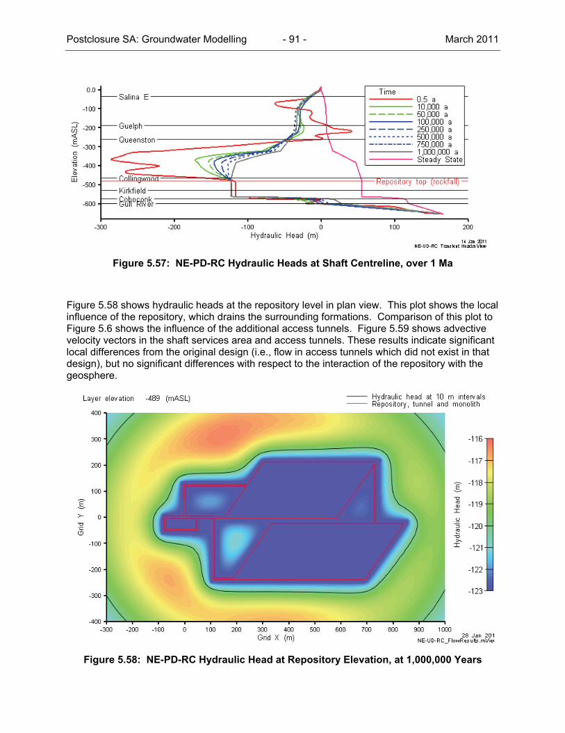
Postclosure SA: Groundwater Modelling - 91 - March 2011
Figure 5.57: NE-PD-RC Hydraulic Heads at Shaft Centreline, over 1 Ma
Figure 5.58 shows hydraulic heads at the repository level in plan view. This plot shows the local influence of the repository, which drains the surrounding formations. Comparison of this plot to Figure 5.6 shows the influence of the additional access tunnels. Figure 5.59 shows advective velocity vectors in the shaft services area and access tunnels. These results indicate significant local differences from the original design (i.e., flow in access tunnels which did not exist in that design), but no significant differences with respect to the interaction of the repository with the geosphere.
Figure 5.58: NE-PD-RC Hydraulic Head at Repository Elevation, at 1,000,000 Years

Postclosure SA: Groundwater Modelling - 92 - March 2011
Figure 5.59: NE-PD-RC Advective Velocity Magnitude and Vectors at Repository Elevation, at 1,000,000 Years
5.11.2 Transport Results
The 1 Ma iso-concentration surfaces are shown in Figure 5.60. The 1 x 10⁻⁷ g/m3 iso-concentration surface on the left hand side of the figure is very similar to its equivalent for the original preliminary design (Figure 5.11), while the 1 x 10⁻⁴ g/m3 iso-concentration surface shows slight differences in the distribution of solute within the repository panels and access tunnels, related to the difference in geometry.
Figure 5.60: NE-PD-RC Cl-36 Concentration Isovolumes at 1,000,000 Years

Postclosure SA: Groundwater Modelling - 93 - March 2011
The time-dependent vertical and horizontal mass flows for the NE-PD-RC case are shown in Figure 5.61. These mass flows are very similar to those of the Reference Case (Figure 5.13), indicating that local differences in groundwater flow and solute transport at the repository level associated with the design modification have little influence on the contaminant mass flow across the Salina F mass transport plane.
Figure 5.61: NE-PD-RC Vertical and Horizontal Cl-36 Mass Flows
5.12 NE-PD-GT5: Increased Shaft Hydraulic Conductivity, Final Preliminary Design
This case is equivalent to NE-GT5 but based on the final preliminary design as shown in Figure 2.5a. The purpose of the case is to assess the difference between groundwater flow and contaminant transport results between the original preliminary design in Figure 2.5b and the final preliminary design in Figure 2.5a, and to assess the sensitivity of the results to changes in design. Flow and transport results are presented in the following two sub sections.
5.12.1 Flow Results
The hydraulic head distribution at the repository and the lower part of the shaft (including the asphalt seal zone) for this calculation case is shown in Figure 5.62. Hydraulic heads in this figure are indistinguishable from the equivalent for the original preliminary design (Figure 5.50). Flow rates up the shaft (not shown) are virtually identical to those of the original preliminary design, indicating that the additional access tunnels in the final preliminary design do not affect the overall groundwater flow from repository level to Shallow Bedrock Groundwater Zone.
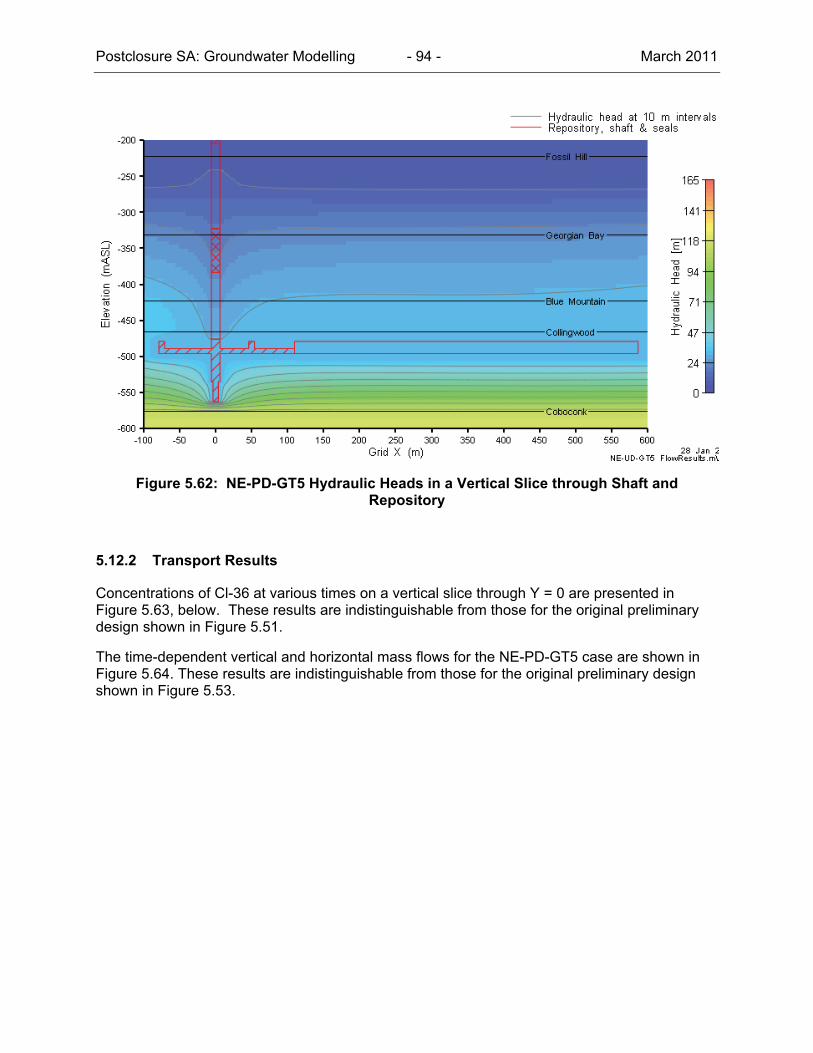
Postclosure SA: Groundwater Modelling - 94 - March 2011
Figure 5.62: NE-PD-GT5 Hydraulic Heads in a Vertical Slice through Shaft and Repository
5.12.2 Transport Results
Concentrations of Cl-36 at various times on a vertical slice through Y = 0 are presented in Figure 5.63, below. These results are indistinguishable from those for the original preliminary design shown in Figure 5.51.
The time-dependent vertical and horizontal mass flows for the NE-PD-GT5 case are shown in Figure 5.64. These results are indistinguishable from those for the original preliminary design shown in Figure 5.53.
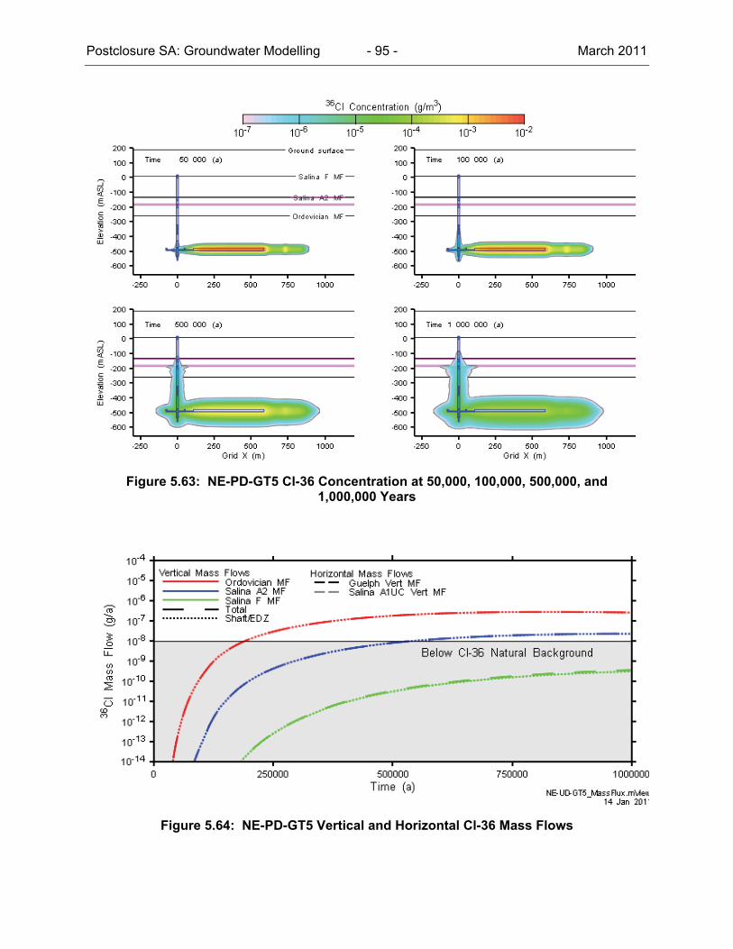
Postclosure SA: Groundwater Modelling - 95 - March 2011
Figure 5.63: NE-PD-GT5 Cl-36 Concentration at 50,000, 100,000, 500,000, and 1,000,000 Years
Figure 5.64: NE-PD-GT5 Vertical and Horizontal Cl-36 Mass Flows
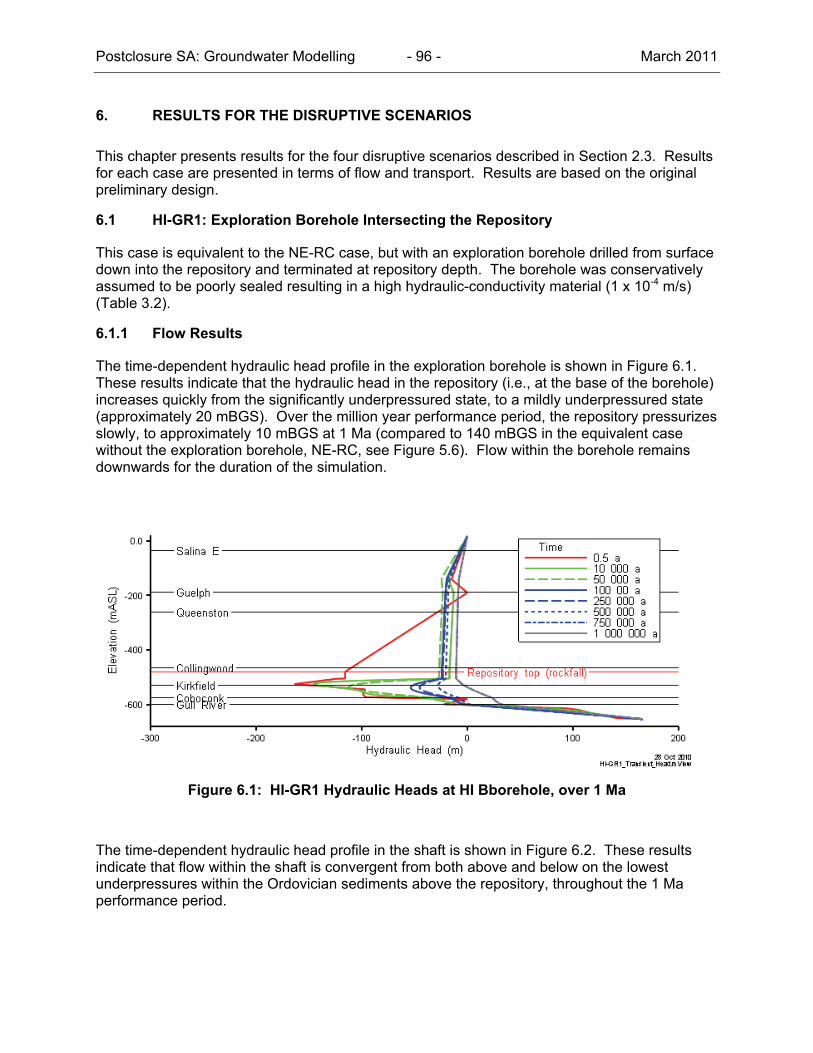
Postclosure SA: Groundwater Modelling - 96 - March 2011
6. RESULTS FOR THE DISRUPTIVE SCENARIOS
This chapter presents results for the four disruptive scenarios described in Section 2.3. Results for each case are presented in terms of flow and transport. Results are based on the original preliminary design.
6.1 HI-GR1: Exploration Borehole Intersecting the Repository
This case is equivalent to the NE-RC case, but with an exploration borehole drilled from surface down into the repository and terminated at repository depth. The borehole was conservatively assumed to be poorly sealed resulting in a high hydraulic-conductivity material (1 x 10⁻⁴ m/s) (Table 3.2).
6.1.1 Flow Results
The time-dependent hydraulic head profile in the exploration borehole is shown in Figure 6.1. These results indicate that the hydraulic head in the repository (i.e., at the base of the borehole) increases quickly from the significantly underpressured state, to a mildly underpressured state (approximately 20 mBGS). Over the million year performance period, the repository pressurizes slowly, to approximately 10 mBGS at 1 Ma (compared to 140 mBGS in the equivalent case without the exploration borehole, NE-RC, see Figure 5.6). Flow within the borehole remains downwards for the duration of the simulation.
Figure 6.1: HI-GR1 Hydraulic Heads at HI Bborehole, over 1 Ma
The time-dependent hydraulic head profile in the shaft is shown in Figure 6.2. These results indicate that flow within the shaft is convergent from both above and below on the lowest underpressures within the Ordovician sediments above the repository, throughout the 1 Ma performance period.
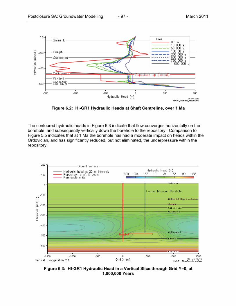
Postclosure SA: Groundwater Modelling - 97 - March 2011
Figure 6.2: HI-GR1 Hydraulic Heads at Shaft Centreline, over 1 Ma
The contoured hydraulic heads in Figure 6.3 indicate that flow converges horizontally on the borehole, and subsequently vertically down the borehole to the repository. Comparison to Figure 5.5 indicates that at 1 Ma the borehole has had a moderate impact on heads within the Ordovician, and has significantly reduced, but not eliminated, the underpressure within the repository.
Figure 6.3: HI-GR1 Hydraulic Head in a Vertical Slice through Grid Y=0, at 1,000,000 Years
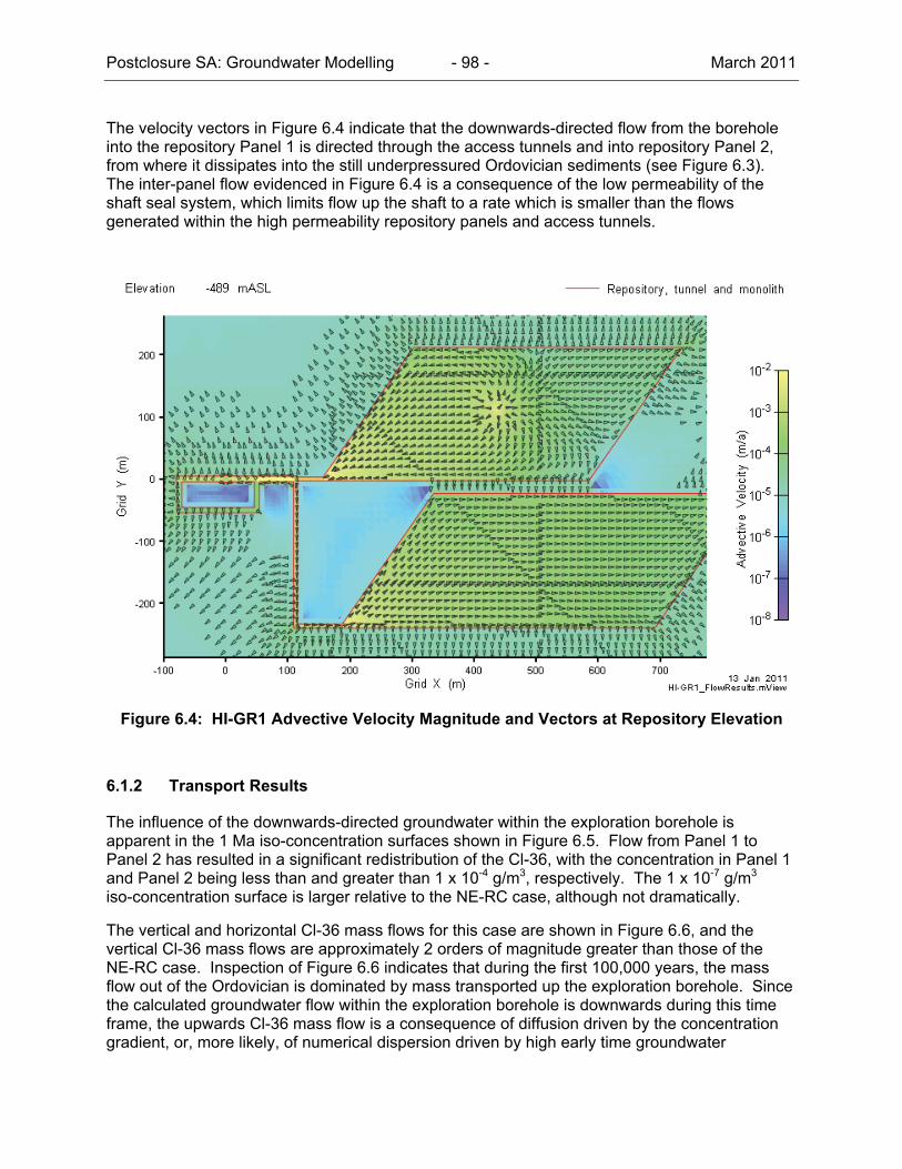
Postclosure SA: Groundwater Modelling - 98 - March 2011
The velocity vectors in Figure 6.4 indicate that the downwards-directed flow from the borehole into the repository Panel 1 is directed through the access tunnels and into repository Panel 2, from where it dissipates into the still underpressured Ordovician sediments (see Figure 6.3). The inter-panel flow evidenced in Figure 6.4 is a consequence of the low permeability of the shaft seal system, which limits flow up the shaft to a rate which is smaller than the flows generated within the high permeability repository panels and access tunnels.
Figure 6.4: HI-GR1 Advective Velocity Magnitude and Vectors at Repository Elevation
6.1.2 Transport Results
The influence of the downwards-directed groundwater within the exploration borehole is apparent in the 1 Ma iso-concentration surfaces shown in Figure 6.5. Flow from Panel 1 to Panel 2 has resulted in a significant redistribution of the Cl-36, with the concentration in Panel 1 and Panel 2 being less than and greater than 1 x 10⁻⁴ g/m3, respectively. The 1 x 10⁻⁷ g/m3
iso-concentration surface is larger relative to the NE-RC case, although not dramatically.
The vertical and horizontal Cl-36 mass flows for this case are shown in Figure 6.6, and the vertical Cl-36 mass flows are approximately 2 orders of magnitude greater than those of the NE-RC case. Inspection of Figure 6.6 indicates that during the first 100,000 years, the mass flow out of the Ordovician is dominated by mass transported up the exploration borehole. Since the calculated groundwater flow within the exploration borehole is downwards during this time frame, the upwards Cl-36 mass flow is a consequence of diffusion driven by the concentration gradient, or, more likely, of numerical dispersion driven by high early time groundwater

Postclosure SA: Groundwater Modelling - 99 - March 2011
velocities (inferred from Figure 6.1). By 250,000 years and onward to 1 Ma, the vertical Cl-36 mass flow out of the Ordovician is dominated by the shaft/EDZ, which is consistent with downwards-flowing groundwater within the borehole. The vertical Cl-36 mass flows at all three considered elevations remain below the natural Cl-36 background deposition rate, and the horizontal Cl-36 mass flows within the Guelph and Salina A1UC are below the plot cut off value.
Figure 6.5: HI-GR1 Cl-36 Concentration Isovolumes at 1,000,000 Years
Figure 6.6: HI-GR1 Vertical and Horizontal Cl-36 Mass Flows
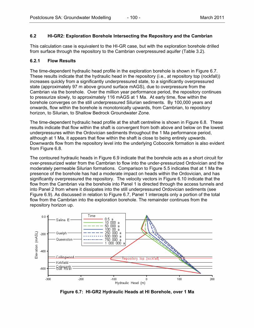
Postclosure SA: Groundwater Modelling - 100 - March 2011
6.2 HI-GR2: Exploration Borehole Intersecting the Repository and the Cambrian
This calculation case is equivalent to the HI-GR case, but with the exploration borehole drilled from surface through the repository to the Cambrian overpressured aquifer (Table 3.2).
6.2.1 Flow Results
The time-dependent hydraulic head profile in the exploration borehole is shown in Figure 6.7. These results indicate that the hydraulic head in the repository (i.e., at repository top (rockfall)) increases quickly from a significantly underpressured state, to a significantly overpressured state (approximately 97 m above ground surface mAGS), due to overpressure from the Cambrian via the borehole. Over the million year performance period, the repository continues to pressurize slowly, to approximately 116 mAGS at 1 Ma. At early time, flow within the borehole converges on the still underpressured Silurian sediments. By 100,000 years and onwards, flow within the borehole is monotonically upwards, from Cambrian, to repository horizon, to Silurian, to Shallow Bedrock Groundwater Zone.
The time-dependent hydraulic head profile at the shaft centreline is shown in Figure 6.8. These results indicate that flow within the shaft is convergent from both above and below on the lowest underpressures within the Ordovician sediments throughout the 1 Ma performance period, although at 1 Ma, it appears that flow within the shaft is close to being entirely upwards. Downwards flow from the repository level into the underlying Coboconk formation is also evident from Figure 6.8.
The contoured hydraulic heads in Figure 6.9 indicate that the borehole acts as a short circuit for over-pressurized water from the Cambrian to flow into the under-pressurized Ordovician and the moderately permeable Silurian formations. Comparison to Figure 5.5 indicates that at 1 Ma the presence of the borehole has had a moderate impact on heads within the Ordovician, and has significantly overpressured the repository. The velocity vectors in Figure 6.10 indicate that the flow from the Cambrian via the borehole into Panel 1 is directed through the access tunnels and into Panel 2 from where it dissipates into the still underpressured Ordovician sediments (see Figure 6.9). As discussed in relation to Figure 6.7, Panel 1 intercepts only a portion of the total flow from the Cambrian into the exploration borehole. The remainder continues from the repository horizon up.
Figure 6.7: HI-GR2 Hydraulic Heads at HI Borehole, over 1 Ma
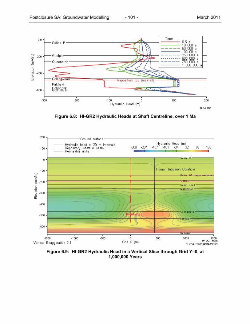
Postclosure SA: Groundwater Modelling - 101 - March 2011
Figure 6.8: HI-GR2 Hydraulic Heads at Shaft Centreline, over 1 Ma
Figure 6.9: HI-GR2 Hydraulic Head in a Vertical Slice through Grid Y=0, at 1,000,000 Years

Postclosure SA: Groundwater Modelling - 102 - March 2011
Figure 6.10: HI-GR2 Advective Velocity Magnitude and Vectors at Repository Elevation
6.2.2 Transport Results
Concentrations of Cl-36 at various times on a vertical slice through the borehole are presented in Figure 6.11 below. These results indicate that a pulse of Cl-36 is transported from the repository up the exploration borehole, where it is expelled outwards into the moderately permeable Silurian formations. Concentrations within these formations are decreasing over the majority of the 1 Ma performance period.
The iso-concentration volumes and plan view concentration contours in the Guelph Formation and in the Salina A1 upper carbonate are shown in Figure 6.12 and Figure 6.13, respectively. Note that the scale of the 1 x 10⁻⁷ g/m3 iso-concentration volume plot has been adjusted in the left pane of Figure 6.12 in order to show the full extent of this concentration within the Guelph Formation (i.e., the figure is more zoomed out than other comparable figures). These results indicate that by 1 Ma, the Cl-36 concentration in both panels is below 1 x 10⁻⁴ g/m3, and that a large proportion of the Cl-36 mass has been expelled upwards through the borehole into the moderately permeable Silurian formations.
The total vertical and horizontal mass flow results shown in Figure 6.14 help to explain these results. Total vertical Cl-36 mass flow out of the Ordovician peaks at 1 x 10⁻² g/a, virtually at time zero, while the peak mass flow into the Shallow Bedrock Groundwater Zone occurs at approximately 100,000 years, at a rate that is two orders of magnitude lower. The difference is made up of the horizontal Cl-36 mass flow within the Guelph (black dashed line) and to a much lesser extent the Salina A1 upper carbonate (gray dashed line). To improve the readability of the figure, only total vertical mass flows are shown, which are dominated by the borehole.
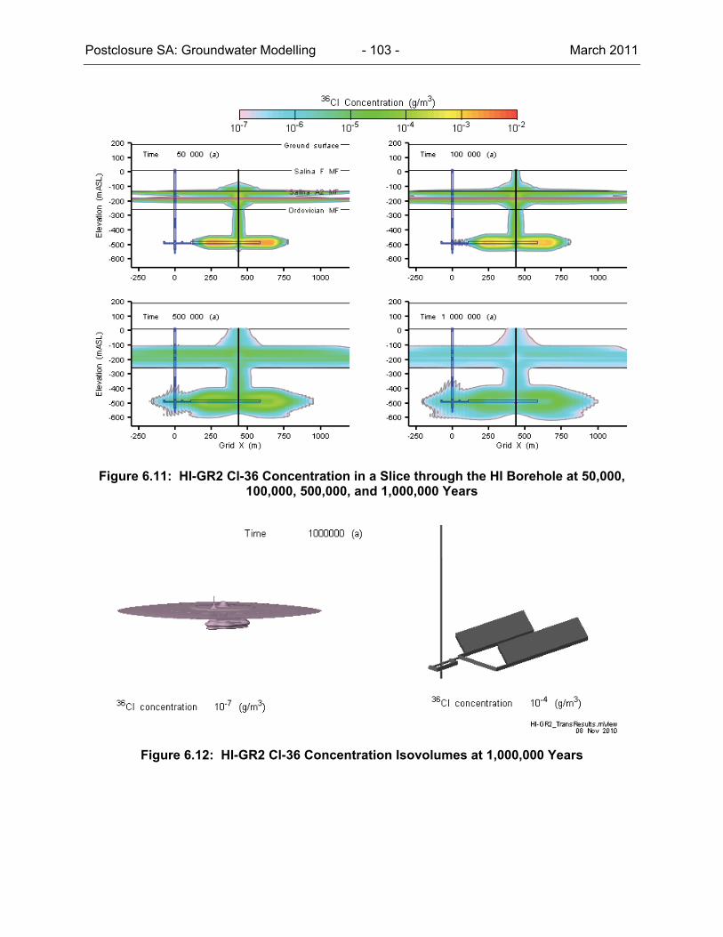
Postclosure SA: Groundwater Modelling - 103 - March 2011
Figure 6.11: HI-GR2 Cl-36 Concentration in a Slice through the HI Borehole at 50,000, 100,000, 500,000, and 1,000,000 Years
Figure 6.12: HI-GR2 Cl-36 Concentration Isovolumes at 1,000,000 Years
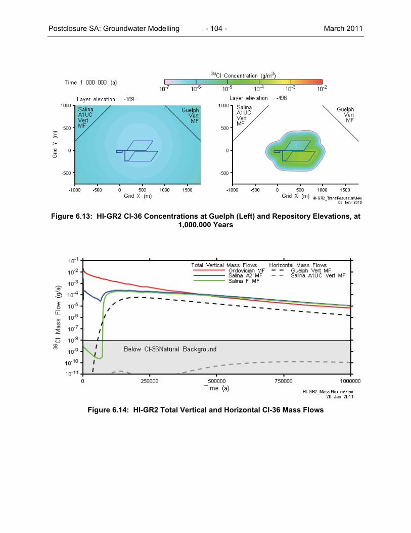
Postclosure SA: Groundwater Modelling - 104 - March 2011
Figure 6.13: HI-GR2 Cl-36 Concentrations at Guelph (Left) and Repository Elevations, at 1,000,000 Years
Figure 6.14: HI-GR2 Total Vertical and Horizontal Cl-36 Mass Flows
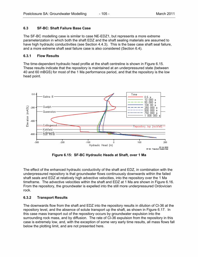
Postclosure SA: Groundwater Modelling - 105 - March 2011
6.3 SF-BC: Shaft Failure Base Case
The SF-BC modelling case is similar to case NE-EDZ1, but represents a more extreme parameterization in which both the shaft EDZ and the shaft sealing materials are assumed to have high hydraulic conductivities (see Section 4.4.3). This is the base case shaft seal failure, and a more extreme shaft seal failure case is also considered (Section 6.4).
6.3.1 Flow Results
The time-dependent hydraulic head profile at the shaft centreline is shown in Figure 6.15. These results indicate that the repository is maintained at an underpressured state (between 40 and 60 mBGS) for most of the 1 Ma performance period, and that the repository is the low head point.
Figure 6.15: SF-BC Hydraulic Heads at Shaft, over 1 Ma
The effect of the enhanced hydraulic conductivity of the shaft and EDZ, in combination with the underpressured repository is that groundwater flows continuously downwards within the failed shaft seals and EDZ at relatively high advective velocities, into the repository over the 1 Ma timeframe. The advective velocities within the shaft and EDZ at 1 Ma are shown in Figure 6.16. From the repository, the groundwater is expelled into the still more underpressured Ordovician rock.
6.3.2 Transport Results
The downwards flow from the shaft and EDZ into the repository results in dilution of Cl-36 at the repository level, and the absence of solute transport up the shaft, as shown in Figure 6.17. In this case mass transport out of the repository occurs by groundwater expulsion into the surrounding rock mass, and by diffusion. The rate of Cl-36 expulsion from the repository in this case is extremely low, and, with the exception of some very early time results, all mass flows fall below the plotting limit, and are not presented here.
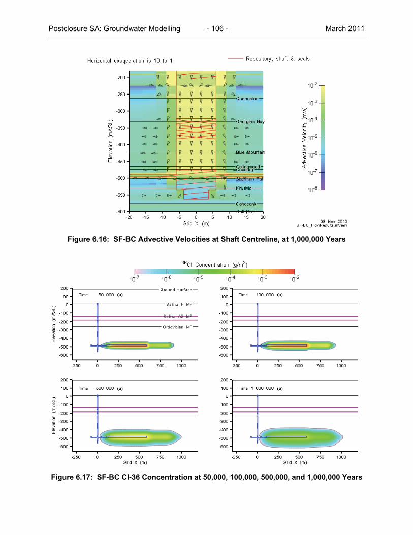
Postclosure SA: Groundwater Modelling - 106 - March 2011
Figure 6.16: SF-BC Advective Velocities at Shaft Centreline, at 1,000,000 Years
Figure 6.17: SF-BC Cl-36 Concentration at 50,000, 100,000, 500,000, and 1,000,000 Years

Postclosure SA: Groundwater Modelling - 107 - March 2011
6.4 SF-ED: Shaft Failure Extra Degradation
The results for this case were very similar to those for the SF-BC case, with groundwater flowing downwards in the shaft towards the repository, throughout the performance period. All Cl-36 mass flows were below the plotting limit.
6.5 BH-BC: Poorly Sealed Borehole
The DGR site will have several deep boreholes around the repository, used for site characterization initially and for monitoring during and after operation. These boreholes will not intersect the repository itself, but will be some distance away. In all cases, the boreholes are licensed through the Ontario Ministry of Natural Resources and they will respect the exclusion zone around the repository footprint. Furthermore, they will be appropriately sealed at the end of their useful lifetime. Consequently, they will have no effect on the performance of the system.
However, if a deep borehole were not properly sealed, then it could provide a small but permeable pathway for the migration of contaminants from the repository. The BH-BC case therefore analyzes a poorly sealed exploration borehole in proximity to the site. The borehole location is approximately that of the DGR-2 site investigation borehole.
6.5.1 Flow Results
The time-dependent hydraulic head profile in the exploration borehole is shown in Figure 6.18. These results indicate that in early time, groundwater within the borehole discharges to the underpressured Silurian rock. Beyond approximately 50,000 years, upwards-directed groundwater flow occurs continuously within the borehole from the Cambrian to the Shallow Bedrock Groundwater Zone.
Figure 6.18: BH-BC Hydraulic Heads at Exploration Borehole, over 1 Ma

Postclosure SA: Groundwater Modelling - 108 - March 2011
The time-dependent hydraulic head profile at the shaft centreline is shown in Figure 6.19. These results indicate, when compared to those of Figure 5.4, only a minor impact of the borehole on the time-dependent hydraulic head in the repository relative to the Reference Case (NE-RC). As shown in Figure 6.20, the repository is still significantly underpressured at 1 Ma and groundwater is flowing outwards from the borehole. In general, in reference to Figure 6.18, the Ordovician sediments intercept a very small proportion of the groundwater flowing upwards within the borehole, while the moderately permeable Silurian formations intercept an appreciable proportion (evidenced by the change in gradient at this horizon in Figure 6.18).
Figure 6.19: BH-BC Hydraulic Heads at Shaft Centreline, over 1 Ma
Figure 6.20: BH-BC Hydraulic Head at Repository Elevation, at 1,000,000 Years
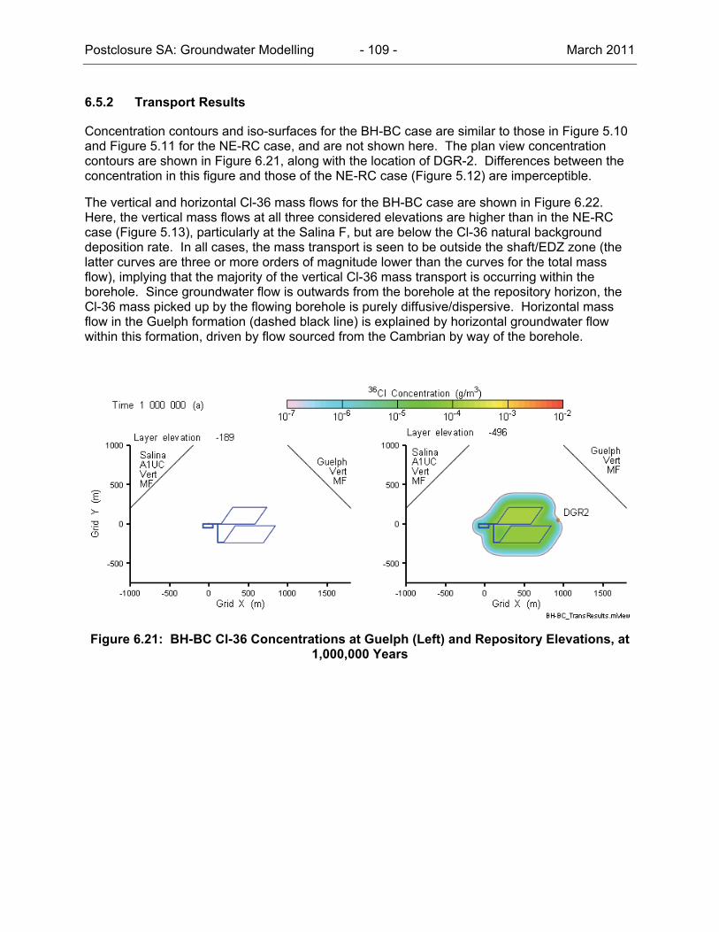
Postclosure SA: Groundwater Modelling - 109 - March 2011
6.5.2 Transport Results
Concentration contours and iso-surfaces for the BH-BC case are similar to those in Figure 5.10 and Figure 5.11 for the NE-RC case, and are not shown here. The plan view concentration contours are shown in Figure 6.21, along with the location of DGR-2. Differences between the concentration in this figure and those of the NE-RC case (Figure 5.12) are imperceptible.
The vertical and horizontal Cl-36 mass flows for the BH-BC case are shown in Figure 6.22. Here, the vertical mass flows at all three considered elevations are higher than in the NE-RC case (Figure 5.13), particularly at the Salina F, but are below the Cl-36 natural background deposition rate. In all cases, the mass transport is seen to be outside the shaft/EDZ zone (the latter curves are three or more orders of magnitude lower than the curves for the total mass flow), implying that the majority of the vertical Cl-36 mass transport is occurring within the borehole. Since groundwater flow is outwards from the borehole at the repository horizon, the Cl-36 mass picked up by the flowing borehole is purely diffusive/dispersive. Horizontal mass flow in the Guelph formation (dashed black line) is explained by horizontal groundwater flow within this formation, driven by flow sourced from the Cambrian by way of the borehole.
Figure 6.21: BH-BC Cl-36 Concentrations at Guelph (Left) and Repository Elevations, at 1,000,000 Years
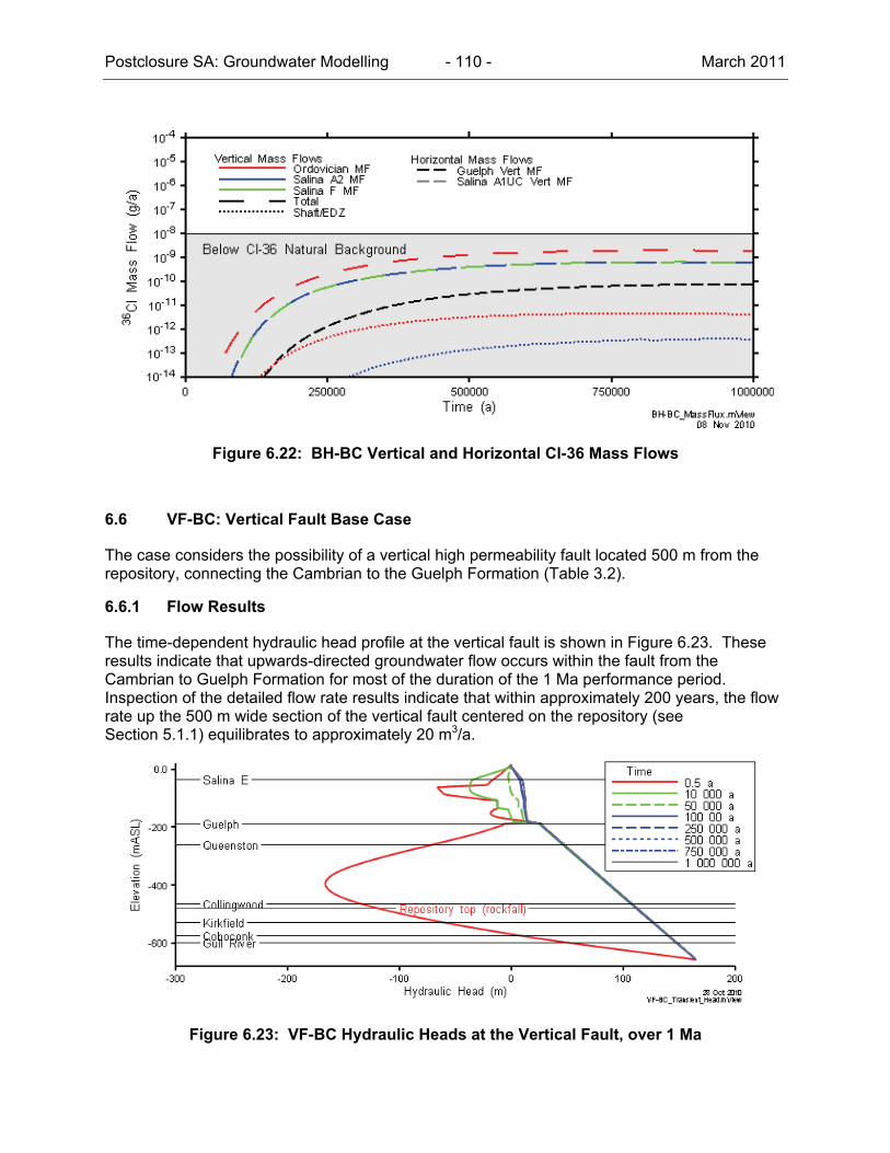
Postclosure SA: Groundwater Modelling - 110 - March 2011
Figure 6.22: BH-BC Vertical and Horizontal Cl-36 Mass Flows
6.6 VF-BC: Vertical Fault Base Case
The case considers the possibility of a vertical high permeability fault located 500 m from the repository, connecting the Cambrian to the Guelph Formation (Table 3.2).
6.6.1 Flow Results
The time-dependent hydraulic head profile at the vertical fault is shown in Figure 6.23. These results indicate that upwards-directed groundwater flow occurs within the fault from the Cambrian to Guelph Formation for most of the duration of the 1 Ma performance period. Inspection of the detailed flow rate results indicate that within approximately 200 years, the flow rate up the 500 m wide section of the vertical fault centered on the repository (see Section 5.1.1) equilibrates to approximately 20 m3/a.
Figure 6.23: VF-BC Hydraulic Heads at the Vertical Fault, over 1 Ma

Postclosure SA: Groundwater Modelling - 111 - March 2011
The time-dependent hydraulic head profile at the shaft centreline is shown in Figure 6.24. When compared to those of Figure 5.4, these results indicate only a minor impact of the vertical fault on the time-dependent hydraulic head in the repository, relative to the base case (NE-RC).
Figure 6.24: VF-BC Hydraulic Heads at Shaft Centreline, over 1 Ma
As shown in Figure 6.25 and Figure 6.26, the repository is still significantly underpressured at 1 Ma (120 mBGS), although lateral flow from the fault towards the repository is occurring.
Figure 6.25: VF-BC Hydraulic Head in a Vertical Slice through Grid Y=0

Postclosure SA: Groundwater Modelling - 112 - March 2011
Figure 6.26: VF-BC Hydraulic Head at Repository Elevation, at 1,000,000 Years
6.6.2 Transport Results
The concentration iso-surfaces for the VF-BC case shown in Figure 6.27 are very similar to those in the corresponding figures for the NE-RC case (Figure 5.11). This indicates that, like the BH-BC case, a transmissive feature some distance from the repository (in this case the assumed fault is 500 m away) has a relatively minor effect on mass transport.
Figure 6.27: VF-BC Cl-36 Concentration Isovolumes at 1,000,000 Years
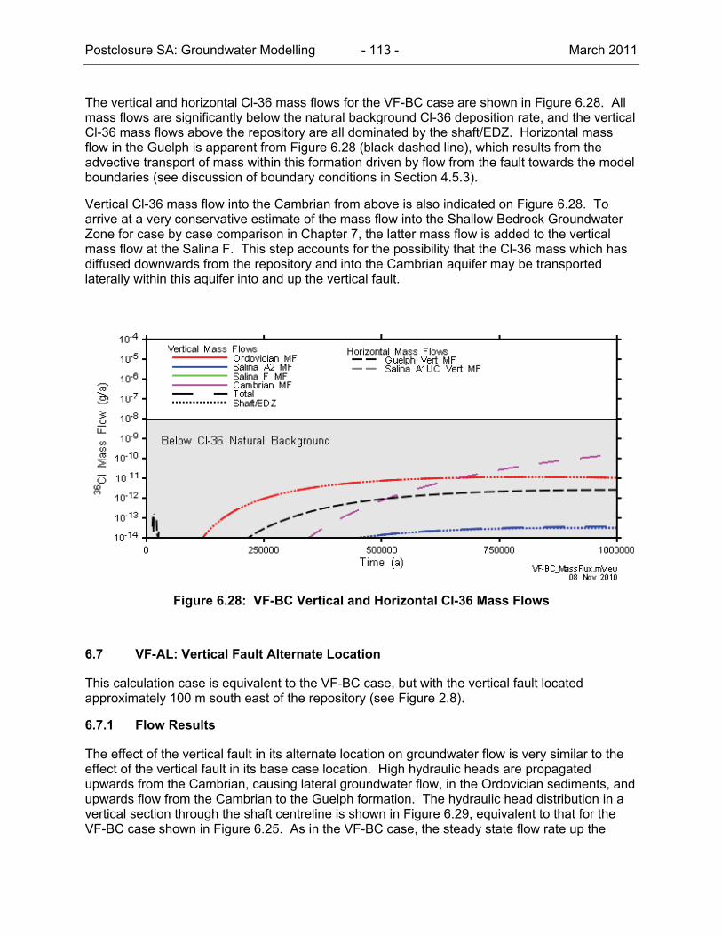
Postclosure SA: Groundwater Modelling - 113 - March 2011
The vertical and horizontal Cl-36 mass flows for the VF-BC case are shown in Figure 6.28. All mass flows are significantly below the natural background Cl-36 deposition rate, and the vertical Cl-36 mass flows above the repository are all dominated by the shaft/EDZ. Horizontal mass flow in the Guelph is apparent from Figure 6.28 (black dashed line), which results from the advective transport of mass within this formation driven by flow from the fault towards the model boundaries (see discussion of boundary conditions in Section 4.5.3).
Vertical Cl-36 mass flow into the Cambrian from above is also indicated on Figure 6.28. To arrive at a very conservative estimate of the mass flow into the Shallow Bedrock Groundwater Zone for case by case comparison in Chapter 7, the latter mass flow is added to the vertical mass flow at the Salina F. This step accounts for the possibility that the Cl-36 mass which has diffused downwards from the repository and into the Cambrian aquifer may be transported laterally within this aquifer into and up the vertical fault.
Figure 6.28: VF-BC Vertical and Horizontal Cl-36 Mass Flows
6.7 VF-AL: Vertical Fault Alternate Location
This calculation case is equivalent to the VF-BC case, but with the vertical fault located approximately 100 m south east of the repository (see Figure 2.8).
6.7.1 Flow Results
The effect of the vertical fault in its alternate location on groundwater flow is very similar to the effect of the vertical fault in its base case location. High hydraulic heads are propagated upwards from the Cambrian, causing lateral groundwater flow, in the Ordovician sediments, and upwards flow from the Cambrian to the Guelph formation. The hydraulic head distribution in a vertical section through the shaft centreline is shown in Figure 6.29, equivalent to that for the VF-BC case shown in Figure 6.25. As in the VF-BC case, the steady state flow rate up the
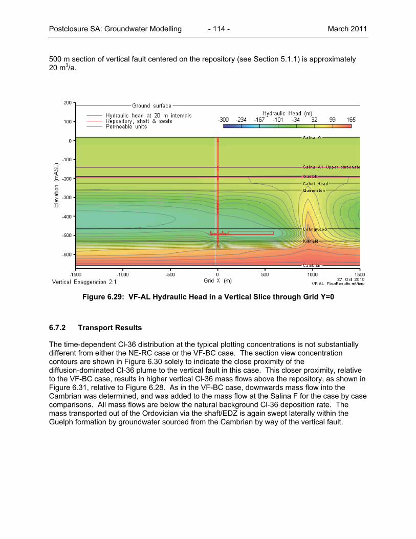
Postclosure SA: Groundwater Modelling - 114 - March 2011
500 m section of vertical fault centered on the repository (see Section 5.1.1) is approximately 20 m3/a.
Figure 6.29: VF-AL Hydraulic Head in a Vertical Slice through Grid Y=0
6.7.2 Transport Results
The time-dependent Cl-36 distribution at the typical plotting concentrations is not substantially different from either the NE-RC case or the VF-BC case. The section view concentration contours are shown in Figure 6.30 solely to indicate the close proximity of the diffusion-dominated Cl-36 plume to the vertical fault in this case. This closer proximity, relative to the VF-BC case, results in higher vertical Cl-36 mass flows above the repository, as shown in Figure 6.31, relative to Figure 6.28. As in the VF-BC case, downwards mass flow into the Cambrian was determined, and was added to the mass flow at the Salina F for the case by case comparisons. All mass flows are below the natural background Cl-36 deposition rate. The mass transported out of the Ordovician via the shaft/EDZ is again swept laterally within the Guelph formation by groundwater sourced from the Cambrian by way of the vertical fault.
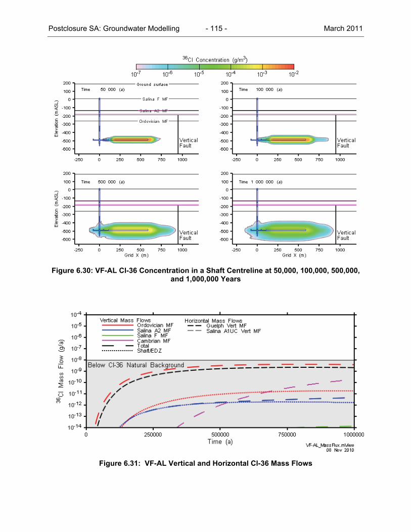
Postclosure SA: Groundwater Modelling - 115 - March 2011
Figure 6.30: VF-AL Cl-36 Concentration in a Shaft Centreline at 50,000, 100,000, 500,000, and 1,000,000 Years
Figure 6.31: VF-AL Vertical and Horizontal Cl-36 Mass Flows
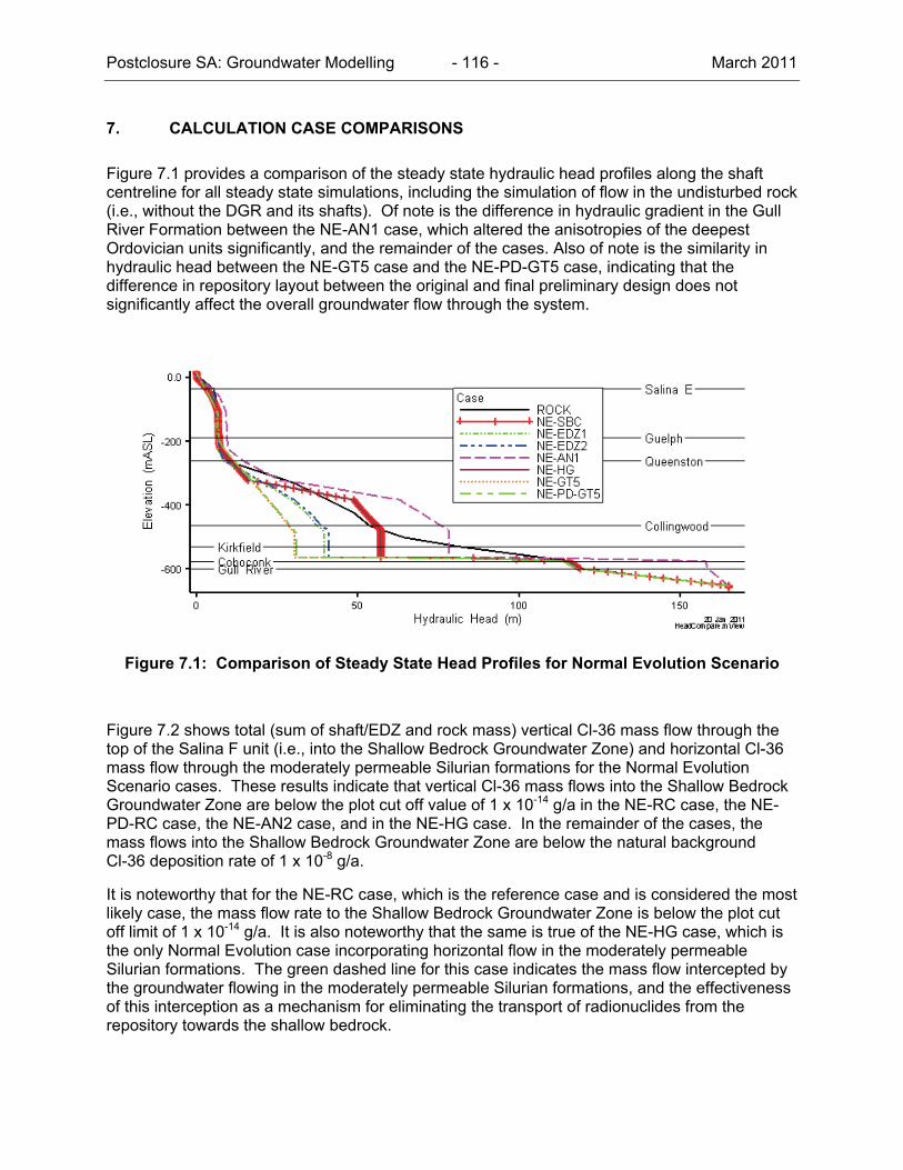
Postclosure SA: Groundwater Modelling - 116 - March 2011
7. CALCULATION CASE COMPARISONS
Figure 7.1 provides a comparison of the steady state hydraulic head profiles along the shaft centreline for all steady state simulations, including the simulation of flow in the undisturbed rock (i.e., without the DGR and its shafts). Of note is the difference in hydraulic gradient in the Gull River Formation between the NE-AN1 case, which altered the anisotropies of the deepest Ordovician units significantly, and the remainder of the cases. Also of note is the similarity in hydraulic head between the NE-GT5 case and the NE-PD-GT5 case, indicating that the difference in repository layout between the original and final preliminary design does not significantly affect the overall groundwater flow through the system.
Figure 7.1: Comparison of Steady State Head Profiles for Normal Evolution Scenario
Figure 7.2 shows total (sum of shaft/EDZ and rock mass) vertical Cl-36 mass flow through the top of the Salina F unit (i.e., into the Shallow Bedrock Groundwater Zone) and horizontal Cl-36 mass flow through the moderately permeable Silurian formations for the Normal Evolution Scenario cases. These results indicate that vertical Cl-36 mass flows into the Shallow Bedrock Groundwater Zone are below the plot cut off value of 1 x 10-14 g/a in the NE-RC case, the NE-PD-RC case, the NE-AN2 case, and in the NE-HG case. In the remainder of the cases, the mass flows into the Shallow Bedrock Groundwater Zone are below the natural background Cl-36 deposition rate of 1 x 10⁻⁸ g/a.
It is noteworthy that for the NE-RC case, which is the reference case and is considered the most likely case, the mass flow rate to the Shallow Bedrock Groundwater Zone is below the plot cut off limit of 1 x 10-14 g/a. It is also noteworthy that the same is true of the NE-HG case, which is the only Normal Evolution case incorporating horizontal flow in the moderately permeable Silurian formations. The green dashed line for this case indicates the mass flow intercepted by the groundwater flowing in the moderately permeable Silurian formations, and the effectiveness of this interception as a mechanism for eliminating the transport of radionuclides from the repository towards the shallow bedrock.

Postclosure SA: Groundwater Modelling - 117 - March 2011
Of the Normal Evolution cases, the three cases with increased permeability of the shaft sealing materials (NE-EDZ1, NE-EDZ2, and NE-GT5) result in the greatest mass flows into the Shallow Bedrock Groundwater Zone, which are still very small.
Figure 7.2: Cl-36 Vertical Mass Flow across the Salina F, and Horizontal Mass Flow in the Silurian for all Normal Evolution Scenario Cases
Figure 7.2 highlights a slight difference in Cl-36 mass flow through the top of the Salina F unit in the NE-GT5 and NE-PD-GT5 cases. This slight difference relates to the slightly different flow path from repository Panel 1 to the shaft in the final preliminary design (see Figure 4.15) relative to the original preliminary design (see Figure 4.13).
Figure 7.3 shows total vertical mass flow through the top of the Salina F unit and horizontal mass transport through the moderately permeable Silurian formations for the Disruptive Scenario cases. These results indicate that the mass flow into the Shallow Bedrock Groundwater Zone peaks at approximately 1 x 10⁻⁴ g/a in the HI-GR2 case, is less than the natural background Cl-36 deposition rate in the BH-BC case, and is below the plot cut off value of 1 x 10-14 g/a in all other cases. Horizontal mass flow in the moderately permeable Silurian formations is observed in the HI-GR2, BH-BC, VF-BC, and VF-AL cases, all driven by lateral flow in these formations sourced from the Cambrian by way of the assessed borehole or fault. While the Disruptive Scenario cases result in higher mass flow rates than the normal evolution cases, their likelihood is considered to be much lower.

Postclosure SA: Groundwater Modelling - 118 - March 2011
Figure 7.3: Cl-36 Vertical Mass Flow across the Salina F, and Horizontal Mass Flow in the Silurian for all Disruptive Scenario Cases
It is noteworthy that the mass flow into the Shallow Bedrock Groundwater Zone falls below the plot cut off value of 1 x 10-14 g/a in both shaft failure cases (SF-BC and SF-ED). As discussed in Section 6.3 and 6.4, this is due to the underpressured state of the repository, and the ongoing downwards flow of groundwater within the failed shaft seals.
Figure 7.4 presents a graphical representation of the peak mass flow for each calculation case, as a general metric of system performance. This plot shows the large range in peak mass flow from case to case, such as the difference between a mass flow that is too low to plot for the NE-RC case and the mass flow approximately eight orders of magnitude higher than the plotting limit for the HI-GR2 case.
Another general metric of system performance is the time of peak mass flow for the Salina F metric. Peak times for all cases were determined to be 1 Ma, except in case HI-GR2 for which a peak time of approximately 125,000 years was determined.
The results of the modelling indicate that the shaft/EDZ system is potentially a significant route for contaminant transport from the facility. In addition to resaturation and gas generation dynamics, which are considered in a companion study (GEOFIRMA and QUINTESSA 2011), the hydraulic properties of the system clearly will dictate the rate and timing of the overall mass release from the facility for any normal evolution of the system. While the case used to test the effectiveness of an enhancement of the shaft sealing system at repository level (NE-EDZ2) showed little value, it was conducted while assuming very high EDZ hydraulic conductivities and a degraded concrete. On the basis that all mass release from the repository is transmitted up the shaft/EDZ, a general conclusion from the modelling is that performance of the shaft sealing system is important.
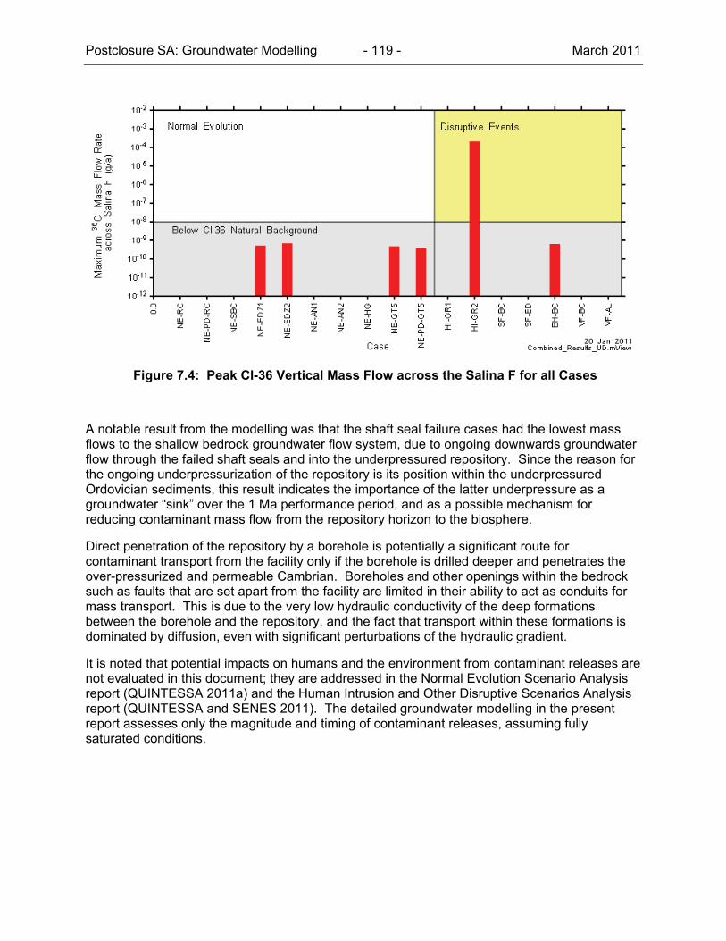
Postclosure SA: Groundwater Modelling - 119 - March 2011
Figure 7.4: Peak Cl-36 Vertical Mass Flow across the Salina F for all Cases
A notable result from the modelling was that the shaft seal failure cases had the lowest mass flows to the shallow bedrock groundwater flow system, due to ongoing downwards groundwater flow through the failed shaft seals and into the underpressured repository. Since the reason for the ongoing underpressurization of the repository is its position within the underpressured Ordovician sediments, this result indicates the importance of the latter underpressure as a groundwater “sink” over the 1 Ma performance period, and as a possible mechanism for reducing contaminant mass flow from the repository horizon to the biosphere.
Direct penetration of the repository by a borehole is potentially a significant route for contaminant transport from the facility only if the borehole is drilled deeper and penetrates the over-pressurized and permeable Cambrian. Boreholes and other openings within the bedrock such as faults that are set apart from the facility are limited in their ability to act as conduits for mass transport. This is due to the very low hydraulic conductivity of the deep formations between the borehole and the repository, and the fact that transport within these formations is dominated by diffusion, even with significant perturbations of the hydraulic gradient.
It is noted that potential impacts on humans and the environment from contaminant releases are not evaluated in this document; they are addressed in the Normal Evolution Scenario Analysis report (QUINTESSA 2011a) and the Human Intrusion and Other Disruptive Scenarios Analysis report (QUINTESSA and SENES 2011). The detailed groundwater modelling in the present report assesses only the magnitude and timing of contaminant releases, assuming fully saturated conditions.
Postclosure SA: Groundwater Modelling - 120 - March 2011
8. UNCERTAINTIES
Uncertainties in results presented in this report arise from a variety of sources, including: the conceptual geosphere model, the numerical modelling approach, and the parameterization of the models in the completely saturated groundwater system. Sources of uncertainty and our approach to dealing with them are discussed in the following subsections.
8.1 Conceptual Model Uncertainty
Our understanding of the geosphere history and future evolution is described in the Geosynthesis report (NWMO 2011), and the postclosure evolution of the system is summarized in the System and Its Evolution report (QUINTESSA 2011b). Specific areas of uncertainty that impact groundwater transport results are listed below, along with how they are currently addressed in this study.
8.1.1 Future Pressures in Ordovician Sediments and Cambrian Sandstone
The present-day underpressure in the low permeability Ordovician sediments above the repository has the potential to act as a groundwater “sink” at least over the 1 Ma duration of the performance period, and to effectively prevent groundwater from flowing from the repository horizon to the Shallow Bedrock Groundwater Zone. Although pressure partitioning due to two-phase flow effects has been identified as a possible source of the measured underpressure, its origin remains uncertain. The conservative approach in assessment of contaminant transport from the repository to the shallow bedrock groundwater system is to ignore the underpressure.
Conversely, the present day overpressure in the Cambrian sandstone below the repository has the potential to act as a driver of upwards groundwater flow through the repository horizon and to the Shallow Bedrock Groundwater Zone. Although this pressure is well established by the site characterization work (INTERA 2011), its origin and evolution is currently unknown. A plausible explanation is that it is due to density driven factors within the Michigan Basin, in which case it would remain approximately constant for timescales of interest (NWMO 2011). The conservative approach in assessment of contaminant transport from the repository to the shallow bedrock groundwater system is to assume the present-day Cambrian overpressure remains indefinitely.
In this study, the most conservative approach has been adopted to account for the uncertainty in the future pressures within the Ordovician sediments and Cambrian sandstone. In all cases, the Cambrian overpressure was assumed to remain indefinitely. In most of the Normal Evolution Scenario (including the NE-SBC) cases, the underpressure in the Ordovician was ignored, and steady-state upward flow throughout the Intermediate and Deep Bedrock Groundwater Zones was assumed. In the reference case (NE-RC), and in cases where flow perturbations such as boreholes and faults were introduced, the Ordovician underpressure was retained as an initial condition, and was allowed to dissipate over the 1 Ma performance period.
Contaminant transport calculations were undertaken using Cl-36, a representative potentially important long-lived radionuclide that is mobile in groundwater. The fact that the Cl-36 mass flow into the Shallow Bedrock Groundwater Zone in both the NE-RC and NE-SBC cases are over 4 order of magnitude below the low Cl-36 natural background deposition rate for the facility footprint (Salina F mass flows in NE-RC and NE-SBC cases are both below the plotting limit in Figure 7.4) indicates that whether steady state or transient conditions are assumed, for the
Postclosure SA: Groundwater Modelling - 121 - March 2011
normal evolution of the facility, mass transport will be dominated by diffusion and the rate of mass transport will be insignificant.
8.1.2 Future Glaciation Events
The primary effects of future glaciation events at the repository horizon are expected to be transient overpressurization during glacial advances followed by dissipation during glacial retreats. Hydrological and chemical impacts will also occur, but primarily in the Shallow Bedrock Groundwater Zone. This is supported by site characterization information and modelling as described in the Geosynthesis report (Section 5.4.6 of NWMO 2011), where the impacts of glaciation on the Ordovician system were determined to be minimal or nonexistent.
In the current study, constant climate conditions were assumed. The results of the current study indicate diffusion-dominated mass transport in the normal evolution of the facility (i.e., without shaft seal failure and human intrusion). The rate of diffusive mass transport has been demonstrated to be insensitive to changes in hydraulic gradients at the repository horizon. Based on this finding, it is possible to assume that glacier-derived transient overpressurization will not have a significant effect on the rate of mass transport, so long as there is no breach of the engineered or natural (geosphere) containment system. This is consistent with the site geological record, which does not show loss of confinement in the Ordovician layers from past glaciation.
8.1.3 Future Horizontal Gradient in the Guelph and Salina A1 Upper Carbonate
The Guelph and Salina A1 upper carbonate are the moderately permeable units in the Intermediate Bedrock Groundwater Zone. Results of the NE-HG case, which incorporated a hydraulic gradient within these units, and the HI-GR2, BH-BC, VF-BC, and VF-AL cases, all of which included a conduit for Cambrian groundwater flow into these units, show that these units will intercept upwards-flowing groundwater and contaminant mass, and prevent it from flowing into the Shallow Bedrock Groundwater Zone. The degree to which this is true will be to some extent controlled by the future magnitude and direction of the hydraulic gradient within these units, which is uncertain. To account for this uncertainty, zero hydraulic gradient in these units was assumed in all cases except the NE-HG, thereby maximizing the contaminant mass flow into the Shallow Bedrock Groundwater Zone.
8.2 Numerical Modelling Assumptions and Approach
The groundwater modelling presented in this report conservatively assumed instant resaturation of the repository and instant dissolution of the entire Cl-36 inventory. In fact, the repository itself will initially be unsaturated and dissolution of the contaminant inventory will not be instantaneous. Due to the low-permeability of the host rock, it will take considerable time to fully resaturate as porewater seeps back into the repository. In addition, gas generated by decomposition of the wastes will also slow down or even stop the resaturation process. These processes were not modelled here. Gas generation and transport modelling results presented in the Gas Modelling report (GEOFIRMA and QUINTESSA 2011) show a long resaturation period (hundreds of thousands or millions of years) where the repository remains mostly or entirely unsaturated. If the time history of resaturation is accounted for, the groundwater transport of radionuclides will be significantly reduced relative to the full dissolution and instantaneous release presented in this report.
Postclosure SA: Groundwater Modelling - 122 - March 2011
In all but one case (the NE-SE case), variable density effects were accounted for only through the use of a calculated environmental head as a bottom (Cambrian) boundary condition, and were not otherwise explicitly included. In the NE-SE case, the observed density profile was included in the numerical model, and its effect modelled explicitly. Comparison of the NE-SE results to the NE-RC results indicates that the contaminant transport from the repository to the Shallow Bedrock Groundwater Zone is insensitive to the density gradient. This is because, for the normal evolution of the system, diffusion is the dominant transport mechanism, and advection, whether driven by boundary conditions or by density gradients, is not a significant contributor to contaminant mass flow.
In general, the groundwater transport results presented in this report are likely conservative. Incorporation of resaturation, gas pressure related effects, and repressurization of transient pressure heads would delay and reduce transport from the repository. Specifically, an important conservative assumption is that saturated hydraulic conductivity is applied to the Ordovician sediments despite the presence of partial gas saturation in these sediments, with associated reduction in pore space available for water flow and associated reduction in relative permeability.
8.3 Parameter Uncertainty
The key parameters in the detailed groundwater modelling undertaken in this study can be summarized as Shaft/EDZ and shaft sealing materials hydraulic conductivity, and geosphere hydraulic conductivity and effective diffusion coefficients. Approaches taken to account for these uncertainties are described below.
8.3.1 Shaft EDZ and Shaft Sealing Materials Hydraulic Conductivity
The results of the modelling indicate that as a subsurface pathway for upward flow and contaminant transport due to the overpressured Cambrian sandstone, the sealed shaft and shaft EDZ is important. To address this uncertainty, extremely conservative assumptions were made about the hydraulic conductivity of these materials in a variety of calculation cases. In all cases but a few, where even higher hydraulic conductivities were assumed, the concrete used for shaft seals and the monolith was assumed to be partially degraded (see Section 4.4 of QUINTESSA and GEOFIRMA 2011), and a high value of hydraulic conductivity was assumed. In the NE-EDZ1 case, the hydraulic conductivity of the shaft EDZ was raised by a factor of 100 relative to the best estimate values. In the NE-GT5 case, the asphalt seal was assumed to have been replaced by additional bentonite/sand, and the bentonite/sand hydraulic conductivity was increased by a factor of 10 relative to the best estimate values. Finally, in the SF-BC and SF-ED cases, the shaft seal materials were all given a very high hydraulic conductivity, relative to the best estimate values (between 100 and 105 times higher).
8.3.2 Geosphere Hydraulic Conductivity and Effective Diffusion Coefficient
Notwithstanding the fact that the results of the modelling indicate advection to be a minor contributor to contaminant mass flow within the host rock, it is prudent to consider geosphere hydraulic conductivities to be key parameters in the modelling. The uncertainty on these values is relatively low because the horizontal hydraulic conductivities are well supported by laboratory testing (INTERA 2011). The anisotropy of hydraulic conductivity (i.e., the ratio of vertical to horizontal) is more uncertain, but this accounted for through a calculation case (NE-AN1) which assumes lower anisotropy than the best estimate values. The results of this case indicate that
Postclosure SA: Groundwater Modelling - 123 - March 2011
the mass flows are insensitive to this parameter, again because of the minor role of advection on overall contaminant mass flow in the host rock.
The current study has demonstrated that in all cases, diffusion is the dominant mechanism for mass transport within the host rock. However, the study has also demonstrated that the host rock is not a significant pathway for mass flow, even in cases where there is a relative short distance within the host rock from the repository to flowing groundwater (i.e., to the vertical fault in the VF-AL and VF-BC cases and to the site characterization borehole in the BH-BC case). The uncertainty on geosphere effective diffusion coefficients is relatively low, because these values are well supported by laboratory testing (INTERA 2011). The anisotropy of effective diffusion coefficient (i.e., the ratio of vertical to horizontal) is more uncertain, but this accounted for through a calculation case (NE-AN2) which assumes lower anisotropy than the best estimate values. The results of this case indicate that the mass flows are insensitive to this parameter, again because only in cases where breach of the repository occurs are there significant contaminant mass flow into the Shallow Bedrock Groundwater Zone.
8.4 Repository Layout
The current assessment considers the preliminary design of the repository and access tunnels. Modifications may occur as the design is moved from preliminary to final. Thus, there is some uncertainty with respect to the final layout.
It is useful to note that the current assessment considered groundwater flow and contaminant transport in two repository layouts, and that the results were comparable in terms of overall performance of the repository. This suggests that the performance of the facility from a groundwater flow perspective is not sensitive to its precise layout.

Postclosure SA: Groundwater Modelling - 124 - March 2011
9. SUMMARY AND CONCLUSIONS
The long-term performance of the proposed L&ILW repository at the Bruce nuclear site has been assessed with the use of numeric models of groundwater flow and transport. Reference and variant cases were undertaken for the Normal Evolution Scenario, and four Disruptive Scenarios. The modelling assessed only the magnitude and timing of contaminant releases in groundwater from the geosphere; gas releases are evaluated in a separate report (GEOFIRMA and QUINTESSA 2011). Furthermore, the potential impacts from contaminant releases on humans and the environment were not evaluated; they are addressed in the Normal Evolution Scenario Analysis report (QUINTESSA 2011a) and the Human Intrusion and Other Disruptive Scenarios Analysis report (QUINTESSA and SENES 2011).
The hydrogeological regime was divided into an upper and a lower part. The model of the upper part, the three-dimensional simplified upper (3DSU) model, was used to simulate the migration of radionuclides in the Shallow Bedrock Groundwater Zone, where advective/dispersive flow towards Lake Huron will be the predominant transport mechanism. The 3DSU model included a water supply well located down-gradient of the repository shafts. The model of the lower zone, the three-dimensional simplified (3DS) model, was used to simulate the migration of radionuclides in the Intermediate and Deep Bedrock Groundwater Zone up to the Shallow Bedrock Groundwater Zone. Mass flow calculated by the 3DS model formed a source term applied at the bottom of the 3DSU model.
Results for the Normal Evolution Scenario’s Reference Case and variant cases all showed excellent containment of contaminants, with no case showing a mass flow to surface greater than the low Cl-36 natural background deposition rate from the atmosphere to the site. These results demonstrate that the extremely low permeability Ordovician and Silurian sediments serve as a highly effective barrier, significantly limiting contaminant migration through groundwater into the biosphere. They also demonstrate the effectiveness of the shaft seal system. A good match between concentrations calculated in the NE-SBC case and equivalent concentrations calculated in a simplified analytical model provides confidence in the results presented in this report.
The results of the modelling indicate that in most Normal Evolution Scenario cases contaminant mass transport from the repository was dominated by diffusion. This conclusion is supported by the similarity in mass flows to the Shallow Bedrock Groundwater Zone in the NE-RC and NE-SBC cases (both below the Cl-36 natural background deposition rate), which incorporated and ignored the present-day underpressures, respectively. This conclusion, supported by the results of the Disruptive Scenario cases, indicates that changes in hydraulic gradient at the repository level brought about by natural processes (e.g., a vertical fault) or anthropogenic events (e.g., a poorly sealed site investigation/monitoring borehole), will not significantly affect the performance of the repository, assuming fully saturated conditions.
The results of the Human Intrusion cases indicate that, in the unlikely event of an exploration borehole being drilled from ground surface to the repository and not sealed, the termination depth will be an important determinant of the significance of the borehole as a conduit for contaminant mass flow to the Shallow Bedrock Groundwater Zone. The modelling suggests that if the borehole is terminated at the repository, then contaminant mass flow out of the repository via and unsealed borehole will be limited, because the repository will remain underpressured for long times. Conversely, if the borehole is drilled through the repository and on to the overpressured Cambrian sandstone, then the contaminant mass flow out of the
Postclosure SA: Groundwater Modelling - 125 - March 2011
repository via an unsealed borehole may be significant. The potential impacts of this and other scenarios are addressed through the SA modelling in a separate report (QUINTESSA and SENES 2011).
Horizontal flow occurred in the moderately permeable Silurian formations as a consequence of their permeability, relative to the remainder of the Intermediate and Deep Bedrock Groundwater Zone, especially in Disruptive Scenario cases, and by virtue of boundary conditions applied in one of the Normal Evolution Scenario cases. These results indicate the importance of horizontal groundwater flow in the moderately permeable Silurian formations as a mechanism to effectively eliminate vertical upward contaminant transport from the repository to the overlying Shallow Bedrock Groundwater Zone.
The results of the modelling indicate that the underpressures within the Ordovician sediments have the potential to act as a groundwater sink over the 1 Ma performance period, and as a mechanism for reducing contaminant mass flow from the repository horizon to the biosphere, even when shaft seal failure is assumed.
The results of the modelling indicate that when the Ordovician underpressures were neglected (i.e., steady state vertical gradients were assumed), the contaminant mass flow to the Shallow Bedrock Groundwater Zone was higher in cases where higher hydraulic conductivities were assigned to the shaft EDZ or to the shaft seal materials. A general conclusion drawn from these results is that that the design of the shaft sealing system is important.
The results of the modelling indicate that the hypothetical water supply well would capture approximately 1% of the mass entering the Shallow Bedrock Groundwater Zone from the repository shaft/EDZ.
Uncertainties in the geosphere conceptual model, modelling assumptions and approaches, and model parameters were all addressed through variant calculation cases that adopted conservative assumptions or values. The two most critical uncertainties are the future pressure distribution within the extremely low permeability Ordovician sediments and within the underlying Cambrian sandstone, relating to uncertainty in the origin of the present-day pressure distribution; and the permeability of the shaft EDZ and the shaft sealing materials.
The cases analyzed in this report are complemented by gas transport modelling and assessment model results presented in companion reports. The results presented in this groundwater modelling report provide insight into the behaviour of the repository system over the 1 Ma performance period, to support the assessment of potential impacts presented in the Postclosure Safety Assessment Report (QUINTESSA et al. 2011a).
Postclosure SA: Groundwater Modelling - 126 - March 2011
10. REFERENCES
Freeze, R. and J. Cherry. 1979. Groundwater. Prentice Hall, New Jersey, USA.
Fritz, P. 1986. Handbook of Environmental Isotope Geochemistry, Vol. 2, The Terrestrial Environment, B. Elsevier Press, New York, USA.
GEOFIRMA and QUINTESSA. 2011. Postclosure Safety Assessment: Gas Modelling. Geofirma Engineering Ltd. and Quintessa Ltd. report for the Nuclear Waste Management Organization NWMO DGR-TR-2011-31 R000. Toronto, Canada.
INTERA. 2011. Descriptive Geosphere Site Model, Deep Geologic Repository. Intera Engineering Ltd. report for the Nuclear Waste Management Organization NWMO DGR-TR-2011-24 R000. Toronto, Canada.
Lanyon, G.W., P. Marschall, M. Fukaya, J. Croise, S. Yamamoto and G. Mayer. 2001. Laboratory Data Compilation Report. Nagra Project Report NBP-00-20. Wettingen, Switzerland.
NWMO. 2011. Geosynthesis. Nuclear Waste Management Organization NWMO DGR-TR-2011-11 R000. Toronto, Canada.
OPG. 2011a. Deep Geologic Repository for Low and Intermediate Level Waste - Environmental Impact Statement. Ontario Power Generation Report 00216-REP-07701-00001 R000. Toronto, Canada.
OPG. 2011b. Deep Geologic Repository for Low and Intermediate Level Waste - Preliminary Safety Report. Ontario Power Generation Report 00216-SR-01320-00001 R000. Toronto, Canada.
QUINTESSA. 2010. Postclosure Safety Assessment Services for OPG’s Proposed Deep Geologic Repository: Project Quality Plan. Quintessa Document QRS-1335B-PQP v3.0. Henley-on-Thames, United Kingdom.
QUINTESSA. 2011a. Postclosure Safety Assessment: Analysis of the Normal Evolution Scenario. Quintessa Ltd. report for the Nuclear Waste Management Organization NWMO DGR-TR-2011-26 R000. Toronto, Canada.
QUINTESSA. 2011b. Postclosure Safety Assessment: System and Its Evolution. Quintessa Ltd. report for the Nuclear Waste Management Organization NWMO DGR-TR-2011-28 R000. Toronto, Canada.
QUINTESSA and GEOFIRMA. 2011. Postclosure Safety Assessment: Data. Quintessa Ltd. and Geofirma Engineering Ltd. report for the Nuclear Waste Management Organization NWMO DGR-TR-2011-32 R000. Toronto, Canada.
QUINTESSA and SENES. 2011. Postclosure Safety Assessment: Analysis of Human Intrusion and Other Disruptive Scenarios. Quintessa Ltd. and SENES Consultants Ltd. report for the Nuclear Waste Management Organization NWMO DGR-TR-2011-27 R000. Toronto, Canada.

Postclosure SA: Groundwater Modelling - 127 - March 2011
QUINTESSA, INTERA and SENES. 2009. Postclosure Safety Assessment (V1) Report.
Quintessa Ltd., Intera Engineering Ltd. and SENES Consultants Ltd. report for the Nuclear Waste Management Organization NWMO DGR-TR-2009-01-R0. Toronto, Canada.
QUINTESSA, GEOFIRMA and SENES. 2011a. Postclosure Safety Assessment. Quintessa Ltd, Geofirma Engineering Ltd and SENES Consultants Ltd. report for the Nuclear Waste Management Organization NWMO DGR-TR-2011-25 R000. Toronto, Canada.
QUINTESSA, SENES and GEOFIRMA. 2011b. Postclosure Safety Assessment: Features, Events and Processes. Quintessa Ltd., SENES Consultants Ltd. and Geofirma Engineering Ltd. report for the Nuclear Waste Management Organization NWMO DGR-TR-2011-29 R000. Toronto, Canada.
Therrien, R. and E.A. Sudicky. 1996. Three-dimensional Analysis of Variably-saturated Flow and Solute Transport in Discretely-fractured Porous Media. Journal of Contaminant Hydrology 23, 1-44.
Therrien, R., R.G. McLaren, E.A. Sudicky, S.M. Panday and V. Guvanasen. 2010. FRAC3DVS-OPG: A Three Dimensional Numeric Model Describing Subsurface Flow and Solute Transport. User’s Guide. Groundwater Simulations Group, Waterloo, Canada.
Postclosure SA: Groundwater Modelling - 128 - March 2011
11. ABBREVIATIONS AND ACRONYMS
BH Poorly Sealed Borehole Scenario
BH-BC Poorly Sealed Borehole Base Case
DGR Deep Geologic Repository
EDZ Excavation Damaged Zone
EIS Environmental Impact Statement
FEPs Features, Events and Processes
HDZ Highly Damaged Zone
HI Human Intrusion Scenario
HI-GR1 Exploration Borehole Intersecting the Repository Case
HI-GR2 Exploration Borehole Intersecting the Repository and the Cambrian Case
L&ILW Low and Intermediate Level Waste
MF Mass Flow
NE Normal Evolution Scenario
NE-AN1 Anisotropy of Bedrock Hydraulic Conductivity Case
NE-AN2 Anisotropy of Bedrock Effective Diffusion Coefficient Case
NE-EDZ1 Increased Hydraulic Conductivity in EDZ Case
NE-EDZ2 Increased Hydraulic Conductivity in EDZ Case with Keyed-in Monolith
NE-GT5 Increased Shaft Seal Hydraulic Conductivity Case
NE-HG Horizontal Gradient in Permeable Silurian Case
NE-PD-GT5 Increased Shaft Seal Hydraulic Conductivity Case for Final Preliminary Design
NE-PD-RC Reference Case for Final Preliminary Design
NE-RC Normal Evolution Scenario - Reference Case
NE-SBC Normal Evolution Scenario - Simplified Base Case
NE-SE Saline Fluid Density Effects Case
NWMO Nuclear Waste Management Organization
OPG Ontario Power Generation Inc.
PD Final Preliminary Design

Postclosure SA: Groundwater Modelling - 129 - March 2011
PSR Preliminary Safety Report
SA Safety Assessment
SF Severe Shaft Seal Failure Scenario
SF-BC Severe Shaft Seal Failure - Base Case
SF-ED Severe Shaft Seal Failure - Extra Degradation Case
UTM Universal Transverse Mercator
VF Vertical Fault Scenario
VF-AL Vertical Fault Scenario - Alternate Location Case
VF-BC Vertical Fault Scenario - Base Case
WI Work Instruction
WWMF Western Waste Management Facility
YMP Yucca Mountain Project

Postclosure SA: Groundwater Modelling - 130 - March 2011
THIS PAGE HAS BEEN LEFT BLANK INTENTIONALLY

Postclosure SA: Groundwater Modelling - 131 - March 2011
APPENDICES

Postclosure SA: Groundwater Modelling - 132 - March 2011
THIS PAGE HAS BEEN LEFT BLANK INTENTIONALLY
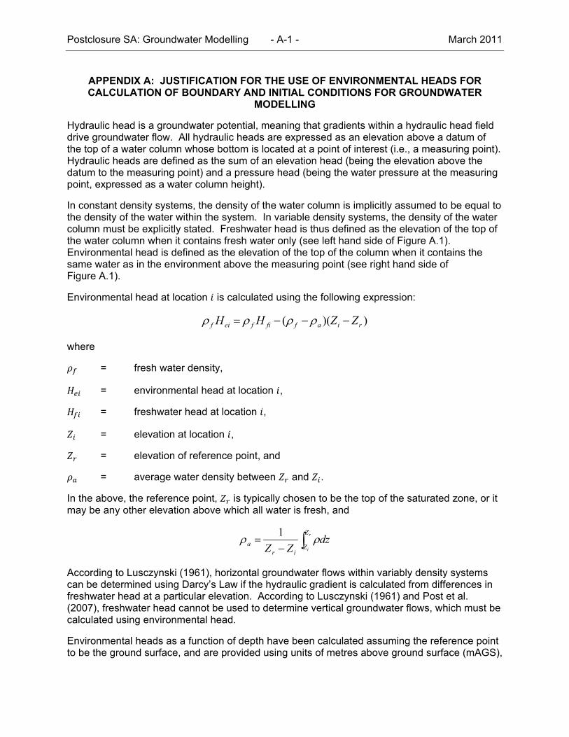
Postclosure SA: Groundwater Modelling - A-1 - March 2011
APPENDIX A: JUSTIFICATION FOR THE USE OF ENVIRONMENTAL HEADS FOR CALCULATION OF BOUNDARY AND INITIAL CONDITIONS FOR GROUNDWATER
MODELLING
Hydraulic head is a groundwater potential, meaning that gradients within a hydraulic head field drive groundwater flow. All hydraulic heads are expressed as an elevation above a datum of the top of a water column whose bottom is located at a point of interest (i.e., a measuring point). Hydraulic heads are defined as the sum of an elevation head (being the elevation above the datum to the measuring point) and a pressure head (being the water pressure at the measuring point, expressed as a water column height).
In constant density systems, the density of the water column is implicitly assumed to be equal to the density of the water within the system. In variable density systems, the density of the water column must be explicitly stated. Freshwater head is thus defined as the elevation of the top of the water column when it contains fresh water only (see left hand side of Figure A.1). Environmental head is defined as the elevation of the top of the column when it contains the same water as in the environment above the measuring point (see right hand side of Figure A.1).
Environmental head at location is calculated using the following expression:
))(( riaffifeif ZZHH
where
= fresh water density,
= environmental head at location ,
= freshwater head at location ,
= elevation at location ,
= elevation of reference point, and
= average water density between and .
In the above, the reference point, is typically chosen to be the top of the saturated zone, or it may be any other elevation above which all water is fresh, and
r
i
Z
Zir
a dzZZ
1
According to Lusczynski (1961), horizontal groundwater flows within variably density systems can be determined using Darcy’s Law if the hydraulic gradient is calculated from differences in freshwater head at a particular elevation. According to Lusczynski (1961) and Post et al. (2007), freshwater head cannot be used to determine vertical groundwater flows, which must be calculated using environmental head.
Environmental heads as a function of depth have been calculated assuming the reference point to be the ground surface, and are provided using units of metres above ground surface (mAGS),
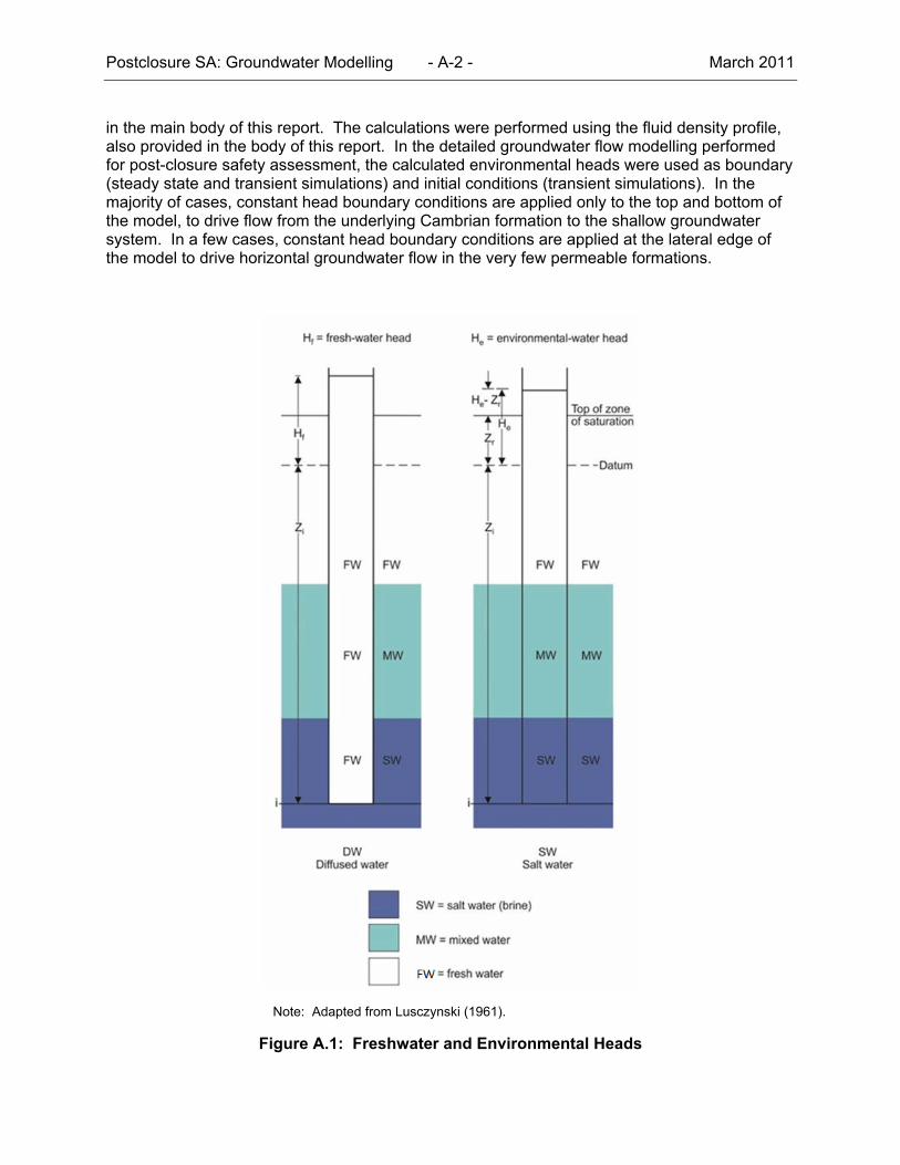
Postclosure SA: Groundwater Modelling - A-2 - March 2011
in the main body of this report. The calculations were performed using the fluid density profile, also provided in the body of this report. In the detailed groundwater flow modelling performed for post-closure safety assessment, the calculated environmental heads were used as boundary (steady state and transient simulations) and initial conditions (transient simulations). In the majority of cases, constant head boundary conditions are applied only to the top and bottom of the model, to drive flow from the underlying Cambrian formation to the shallow groundwater system. In a few cases, constant head boundary conditions are applied at the lateral edge of the model to drive horizontal groundwater flow in the very few permeable formations.
Note: Adapted from Lusczynski (1961).
Figure A.1: Freshwater and Environmental Heads
Postclosure SA: Groundwater Modelling - A-3 - March 2011
Since the critical groundwater flows within these detailed flow models are predominantly vertical (i.e., from the repository to the biosphere), the use of a constant density flow model with environmental heads as boundary and initial conditions is appropriate. Horizontal flows induced by the repository and shaft system are considered to be insensitive to the difference between the applied environmental-head-based boundary conditions, and the freshwater head equivalents, particularly given the lack of lateral constant head boundary conditions.
The most important assumption implicit in the use of the chosen methodology (to use environmental heads calculated from present-day pore-water chemistry as boundary and initial conditions) is that the density profile does will not change significantly over the million year duration of the simulation. Given the very low permeability of the majority of formations, and the consequently very low rate of diffusive and advective transport, this assumption is considered reasonable, particularly in light of the uncertainty regarding the long-term evolution of pressures in the Cambrian formation.
REFERENCES FOR APPENDIX A
Lusczynski, N.J. 1961. Head and Flow of Groundwater of Variable Density, Journal Geophysical Research, Vol. 66, No. 12, 4247-4256.
Post, V., H. Kooi, and C. Simmons. 2007. Using Hydraulic Head Measurements in Variable-Density Ground Water Flow Analyses. Ground Water, Vol. 45, No. 6, 664-671.

Postclosure SA: Groundwater Modelling - A-4 - March 2011
THIS PAGE HAS BEEN LEFT BLANK INTENTIONALLY
Postclosure SA: Groundwater Modelling - B-1 - March 2011
APPENDIX B: FRAC3DVS-OPG
B.1 PURPOSE
FRAC3DVS-OPG provides transient groundwater modelling and contaminant transport in 2D and 3D geometry for saturated variable-density systems, including both equivalent porous medium and discrete fracture networks.
FRAC3DVS-OPG was used to simulate 3D transient groundwater flow and contaminant transport for the postclosure assessment of the DGR. It was used for the following scenarios:
Normal Evolution; Human Intrusion; Severe Shaft Seal Failure; Poorly Sealed Borehole; and Vertical Fault.
The site and repository was represented using an equivalent porous medium model. The variable density capabilities of the code were used in the NE-SE case. The current application did not use the 1D hydromechanical, or discrete-fracture capabilities of the code.
B.2 CODE HISTORY
FRAC3DVS-OPG is a code developed and maintained by Groundwater Simulations Group in Waterloo, Canada.
FRAC3DVS-OPG was originally developed and is commercially available under the name FRAC3DVS (Therrien and Sudicky 1996). The numeric engine is also incorporated into the HydroGeoSphere model (Therrien et al. 2010b). Code development and use has been supported by OPG and NWMO as part of its used fuel technology program, as well as by other commercial and academic users.
The FRAC3DVS-OPG code is a specific QA release of FRAC3DVS maintained by OPG and NWMO. The current version is V1.3.0.
B.3 REQUIREMENTS
FRAC3DVS-OPG is a FORTRAN code and can be compiled to run on 32-bit and 64-bit Windows and Linux operating systems. Specific computational requirements (RAM, processor speed, disc storage) are entirely problem dependent. The current DGR postclosure safety assessment 3DS model requires 64-bit systems with 4 GB of RAM.
FRAC3DVS-OPG is designed for expert users and assumes a high degree of modelling proficiency and access to supporting pre- and post-processing software.
B.4 CAPABILITIES
A full description is provided in Therrien et al. (2010a).
Postclosure SA: Groundwater Modelling - B-2 - March 2011
B.5 LIMITATIONS
FRAC3DVS-OPG is subject to spatial and temporal discretization requirements similar to most Finite-Element and Finite-Difference models. End users of the application are responsible for ensuring that suitable discretizations are specified.
B.6 DOCUMENTATION
B.6.1 Theory
FRAC3DVS-OPG theory is described in Section 2 of Therrien et al. (2010a), as well as Therrien, Sudicky and McLaren (2004), and Therrien and Sudicky (1996).
B.6.2 Requirements Specifications
A formal requirements document is not available. Basic requirements/capabilities are described in Section 1 of Therrien et al. (2010a).
B.6.3 Design Description/Programmer Manual
Numeric implementation is described in Therrien et al. (2010a). Details on overall software development practices and approaches are not described.
B.6.4 Source Code
FRAC3DVS-OPG source code is maintained by Groundwater Simulation Group:
Groundwater Simulations Group 574 Sprucehill Avenue Waterloo, Ontario N2L 4V9
Source code is not distributed with the model.
B.6.5 Verification Reports
Specific verification reports for theory, requirements, design, and code are not available. However, the theory has been presented in peer-reviewed journals, and the base code has had moderately wide commercial use for over a decade.
B.6.6 User Manual
The FRAC3DVS-OPG User Manual is contained in Section 4 of Therrien et al. (2010a).
B.7 VALIDATION
FRAC3DVS-OPG validation test cases are described in Therrien et al. (2010a).
B.8 VERSION TRACKING RECORD
FRAC3DVS-OPG (Version 1.3.0, Build Date 2010 06 03 - 64-bit).

Postclosure SA: Groundwater Modelling - B-3 - March 2011
REFERENCES FOR APPENDIX B
Therrien, R. and E.A. Sudicky. 1996. Three-dimensional Analysis of Variably-saturated Flow and Solute Transport in Discretely-fractured Porous Media. Journal Contaminant Hydrology 23, 1-44.
Therrien, R., E.A. Sudicky and R.G. McLaren. 2004. FRAC3DVS: An Efficient Simulator for Three-dimensional, Saturated-Unsaturated Groundwater Flow and Density-dependent, Chain-Decay Solute Transport in Porous, Discretely-Fractured Porous or Dual-porosity Formations. User’s Guide. University of Waterloo, Canada.
Therrien, R., R.G. McLaren, E.A. Sudicky, S.M. Panday and V. Guvanasen. 2010a. FRAC3DVS-OPG: A Three Dimensional Numeric Model Describing Subsurface Flow and Solute Transport. User’s Guide. University of Waterloo, Ontario.
Therrien, R., R.G. McLaren, E.A. Sudicky and S.M. Panday. 2010b. HydroGeoSphere, A Three-dimensional Numerical Model Describing Fully-integrated Subsurface and Surface Flow and Solute Transport. University of Waterloo, Ontario.

Postclosure SA: Groundwater Modelling - B-4 - March 2011
THIS PAGE HAS BEEN LEFT BLANK INTENTIONALLY
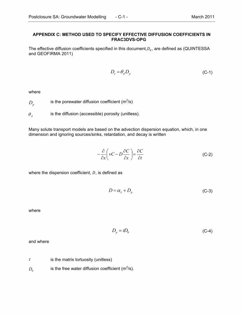
Postclosure SA: Groundwater Modelling - C-1 - March 2011
APPENDIX C: METHOD USED TO SPECIFY EFFECTIVE DIFFUSION COEFFICIENTS IN FRAC3DVS-OPG
The effective diffusion coefficients specified in this document, , are defined as (QUINTESSA and GEOFIRMA 2011)
where
pD is the porewater diffusion coefficient (m2/s)
d is the diffusion (accessible) porosity (unitless).
Many solute transport models are based on the advection dispersion equation, which, in one dimension and ignoring sources/sinks, retardation, and decay is written
where the dispersion coefficient, , is defined as
where
and where
is the matrix tortuosity (unitless)
0D is the free water diffusion coefficient (m2/s).
pde DD (C-1)
t
C
x
CDvC
x
(C-2)
pL DD (C-3)
0DDp (C-4)

Postclosure SA: Groundwater Modelling - C-2 - March 2011
FRAC3DVS-OPG is formulated as above, with input parameters , , and porosity, . Thus, combining equation (C-1) with (C-4), substituting for d , and rearranging, the tortuosity used
for each material used in the model is back-calculated as follows:
For example, the tortuosity, , associated with the diffusion of Cl-36 in the Lucas Formation is calculated to be 0.086 by solving equation (C-5) with eD = 6 x 10-12 m2/s, = 0.07, and
0D =1 x 10⁻⁹ m2/s.
REFERENCES FOR APPENDIX C
QUINTESSA and GEOFIRMA. 2011. Postclosure Safety Assessment: Data. Quintessa Ltd. and Geofirma Engineering Ltd. report for the Nuclear Waste Management Organization NWMO DGR-TR-2011-32 R000. Toronto, Canada.
0D
De
(C-5)

Postclosure SA: Groundwater Modelling - D-1 - March 2011
APPENDIX D: FEP AUDIT OF FRAC3DVS-OPG MODELS FOR THE POSTCLOSURE SAFETY ASSESSMENT

Postclosure SA: Groundwater Modelling - D-2 - March 2011
THIS PAGE HAS BEEN LEFT BLANK INTENTIONALLY

Pos
tclo
sure
SA
: Gro
und
wat
er M
odel
ling
- D
-3 -
M
arch
201
1
FE
P
In
clu
ded
in F
RA
C3D
VS
-OP
G M
od
els
2. IN
TE
RN
AL
FA
CT
OR
S
2.1
Was
te, W
aste
For
m &
Eng
inee
red
Com
pone
nts
2.
1.01
W
aste
inve
ntor
y P
arti
al -
det
aile
d m
odel
ling
cond
ucte
d us
ing
Cl-3
6 so
urce
onl
y
2.1.
01.0
1 R
adio
nucl
ide
cont
ent
2.
1.01
.02
C
hem
ical
con
tent
2.
1.02
W
aste
-for
m c
hara
cter
istic
s
No
- e
ntire
was
te in
vent
ory
of C
l-36
ass
umed
inst
anta
neou
sly
diss
olve
d in
sa
tura
ted
repo
sito
ry a
t t =
0. N
o w
aste
form
or
sour
ce te
rm m
odel
.
2.1.
02.0
1
Met
allic
was
tes
2.
1.02
.02
O
rgan
ic w
aste
s
2.
1.02
.03
N
on-m
etal
lic, i
norg
anic
w
aste
s
2.
1.03
W
aste
-pac
kagi
ng c
hara
cter
istic
s
2.1.
03.0
1 C
onta
iner
s
2.1.
03.0
2 O
verp
acks
2.
1.04
E
mpl
acem
ent r
oom
, acc
ess
tunn
el a
nd
shaf
t & s
ervi
ces
area
cha
ract
eris
tics
2.1.
04.0
1
Roo
fs a
nd w
alls
P
arti
al -
em
plac
emen
t drif
ts g
roup
ed in
to tw
o pa
nels
. Acc
ess
tunn
els
from
sha
ft to
pa
nels
incl
uded
exp
licitl
y.
2.1.
04.0
2 F
loor
s
2.1.
04.0
3 R
ock
bolts
N
o -
not
incl
uded
- im
pact
on
hydr
aulic
s lu
mpe
d w
ith r
epos
itory
ED
Z
2.1.
04.0
4 R
oom
and
clo
sure
wal
ls
Par
tial
- a
lthou
gh p
anel
s ar
e m
odel
led
as c
ontig
uous
voi
d sp
ace,
wal
ls a
re
acco
unte
d fo
r in
the
calc
ulat
ion
of r
epos
itory
voi
d vo
lum
e.
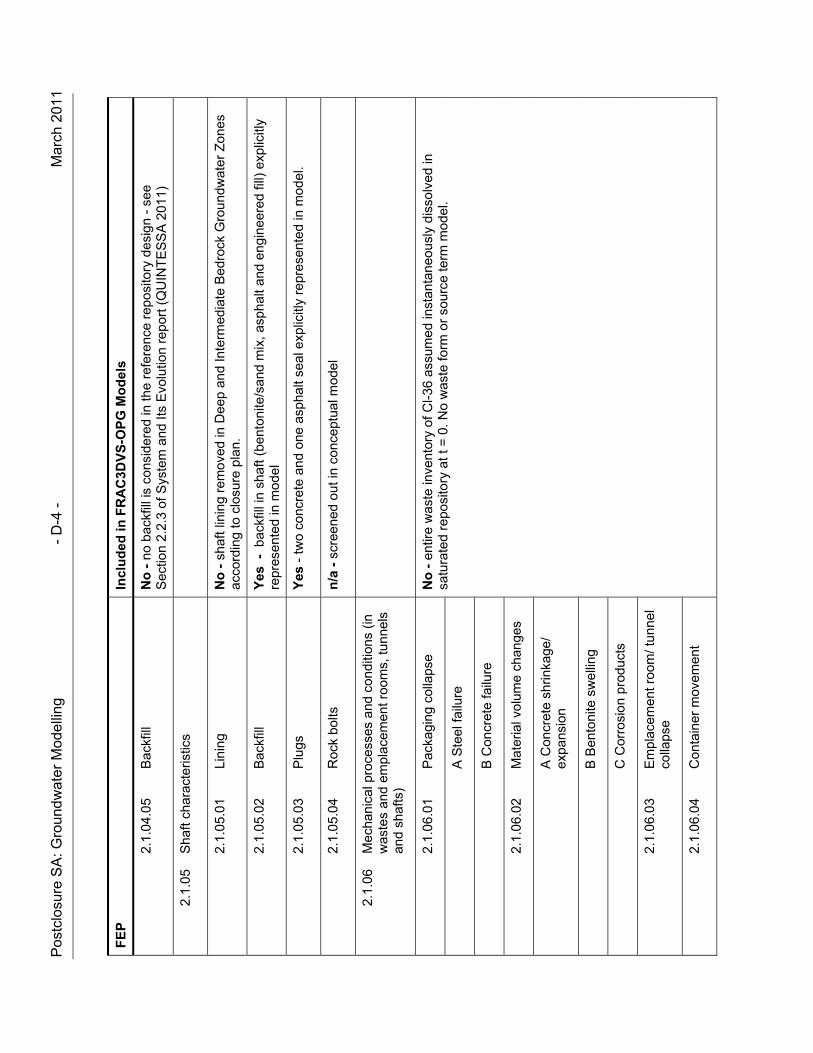
Pos
tclo
sure
SA
: Gro
und
wat
er M
odel
ling
- D
-4 -
M
arch
201
1
FE
P
In
clu
ded
in F
RA
C3D
VS
-OP
G M
od
els
2.1.
04.0
5 B
ackf
ill
No
- n
o ba
ckfil
l is
cons
ider
ed in
the
refe
renc
e re
posi
tory
des
ign
- se
e S
ectio
n 2.
2.3
of S
yste
m a
nd It
s E
volu
tion
repo
rt (
QU
INT
ES
SA
201
1)
2.
1.05
S
haft
char
acte
ristic
s
2.1.
05.0
1 Li
ning
N
o -
sha
ft lin
ing
rem
oved
in D
eep
and
Inte
rmed
iate
Bed
rock
Gro
undw
ater
Zon
es
acco
rdin
g to
clo
sure
pla
n.
2.1.
05.0
2 B
ackf
ill
Yes
- b
ackf
ill in
sha
ft (b
ento
nite
/san
d m
ix,
asph
alt a
nd e
ngin
eere
d fil
l) ex
plic
itly
repr
esen
ted
in m
odel
2.1.
05.0
3 P
lugs
Y
es -
two
conc
rete
and
one
asp
halt
seal
exp
licitl
y re
pres
ente
d in
mod
el.
2.1.
05.0
4 R
ock
bolts
n
/a -
scr
eene
d ou
t in
conc
eptu
al m
odel
2.
1.06
M
echa
nica
l pro
cess
es a
nd c
ondi
tions
(in
w
aste
s an
d em
plac
emen
t roo
ms,
tunn
els
and
shaf
ts)
2.1.
06.0
1 P
acka
ging
col
laps
e N
o -
ent
ire w
aste
inve
ntor
y of
Cl-3
6 a
ssum
ed in
stan
tane
ousl
y di
ssol
ved
in
satu
rate
d re
posi
tory
at t
= 0
. No
was
te fo
rm o
r so
urce
term
mod
el.
A
Ste
el fa
ilure
B
Con
cret
e fa
ilure
2.1.
06.0
2
Mat
eria
l vol
ume
chan
ges
A
Con
cret
e sh
rinka
ge/
expa
nsio
n
B
Ben
toni
te s
wel
ling
C
Cor
rosi
on p
rodu
cts
2.1.
06.0
3
Em
plac
emen
t roo
m/ t
unne
l co
llaps
e
2.1.
06.0
4
Con
tain
er m
ovem
ent

Pos
tclo
sure
SA
: Gro
und
wat
er M
odel
ling
- D
-5 -
M
arch
201
1
FE
P
In
clu
ded
in F
RA
C3D
VS
-OP
G M
od
els
2.1.
06.0
5
Fra
ctur
e fo
rmat
ion
N
o -
mod
elle
d ge
osph
ere
is ti
me
inva
riant
. Con
cret
e se
al p
rope
rtie
s ar
e co
nsis
tent
w
ith d
egra
ded
mat
eria
l.
2.
1.06
.06
Str
ess-
corr
osio
n cr
acki
ng
n/a
- s
cree
ned
out i
n co
ncep
tual
mod
el
2.
1.06
.07
Gas
exp
losi
on
n/a
- s
cree
ned
out i
n co
ncep
tual
mod
el
2.
1.06
.08
Influ
ence
of c
limat
e ch
ange
Y
es -
10
m r
ockf
all i
n th
e re
posi
tory
is a
ttrib
uted
to p
ossi
ble
glac
iatio
n im
pact
s
2.
1.07
H
ydra
ulic
/hyd
roge
olog
ical
pro
cess
es a
nd
cond
ition
s (in
was
tes,
em
plac
emen
t ro
oms,
tunn
els
and
shaf
ts)
2.1.
07.0
1
Res
atur
atio
n/de
satu
ratio
n
No
- r
epos
itory
is c
onsi
dere
d to
be
inst
anta
neou
sly
satu
rate
d at
t =
0.
2.1.
07.0
2 W
ater
flow
Y
es -
exp
licitl
y m
odel
led
2.1.
07.0
3
Gas
-med
iate
d w
ater
flow
N
o -
impa
cts
of p
ossi
ble
gas
satu
ratio
n in
geo
sphe
re a
nd E
BS
not
incl
uded
2.1.
07.0
4
Fai
lure
of d
rain
age
syst
em
n/a
- s
cree
ned
out i
n co
ncep
tual
mod
el
2.1.
07.0
5 F
ract
urin
g of
rep
osito
ry
com
pone
nts
due
to
hydr
aulic
pre
ssur
e
n/a
- s
cree
ned
out i
n co
ncep
tual
mod
el
2.1.
07.0
6
Cou
pled
hyd
raul
ic
proc
esse
s in
clud
ing
tem
pera
ture
, che
mic
al o
r el
ectr
ical
gra
dien
ts
n/a
- s
cree
ned
out i
n co
ncep
tual
mod
el
2.1.
07.0
7
Influ
ence
of c
limat
e ch
ange
Y
es -
pro
pert
ies
of u
pper
sha
ft in
3D
SU
mod
el r
efle
ct d
egra
ded
stat
e du
e to
gl
acia
l-int
ergl
acia
l cyc
ling
and
the
asso
ciat
ed c
hem
ical
/geo
chem
ical
impa
cts.
2.
1.08
C
hem
ical
/geo
chem
ical
pro
cess
es a
nd
cond
ition
s (in
was
tes,
em
plac
emen
t ro
oms,
tunn
els
and
shaf
ts)
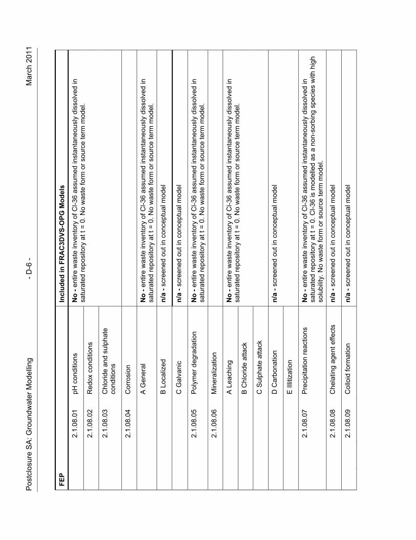
Pos
tclo
sure
SA
: Gro
und
wat
er M
odel
ling
- D
-6 -
M
arch
201
1
FE
P
In
clu
ded
in F
RA
C3D
VS
-OP
G M
od
els
2.1.
08.0
1 pH
con
ditio
ns
No
- e
ntire
was
te in
vent
ory
of C
l-36
ass
umed
inst
anta
neou
sly
diss
olve
d in
sa
tura
ted
repo
sito
ry a
t t =
0. N
o w
aste
form
or
sour
ce te
rm m
odel
.
2.
1.08
.02
Red
ox c
ondi
tions
2.1.
08.0
3 C
hlor
ide
and
sulp
hate
co
nditi
ons
2.1.
08.0
4 C
orro
sion
A
Gen
eral
N
o -
ent
ire w
aste
inve
ntor
y of
Cl-3
6 a
ssum
ed in
stan
tane
ousl
y di
ssol
ved
in
satu
rate
d re
posi
tory
at t
= 0
. No
was
te fo
rm o
r so
urce
term
mod
el.
B
Loc
aliz
ed
n/a
- s
cree
ned
out i
n co
ncep
tual
mod
el
C
Gal
vani
c n
/a -
scr
eene
d ou
t in
conc
eptu
al m
odel
2.1.
08.0
5 P
olym
er d
egra
datio
n N
o -
ent
ire w
aste
inve
ntor
y of
Cl-3
6 a
ssum
ed in
stan
tane
ousl
y di
ssol
ved
in
satu
rate
d re
posi
tory
at t
= 0
. No
was
te fo
rm o
r so
urce
term
mod
el.
2.1.
08.0
6 M
iner
aliz
atio
n
A
Lea
chin
g N
o -
ent
ire w
aste
inve
ntor
y of
Cl-3
6 a
ssum
ed in
stan
tane
ousl
y di
ssol
ved
in
satu
rate
d re
posi
tory
at t
= 0
. No
was
te fo
rm o
r so
urce
term
mod
el.
B
Chl
orid
e at
tack
C
Sul
phat
e at
tack
D
Car
bona
tion
n/a
- s
cree
ned
out i
n co
ncep
tual
mod
el
E
Illit
izat
ion
2.1.
08.0
7 P
reci
pita
tion
reac
tions
N
o -
ent
ire w
aste
inve
ntor
y of
Cl-3
6 a
ssum
ed in
stan
tane
ousl
y di
ssol
ved
in
satu
rate
d re
posi
tory
at t
= 0
. Cl-3
6 is
mod
elle
d as
a n
on-s
orbi
ng s
peci
es w
ith h
igh
solu
bilit
y. N
o w
aste
form
or
sour
ce te
rm m
odel
.
2.1.
08.0
8 C
hela
ting
agen
t effe
cts
n/a
- s
cree
ned
out i
n co
ncep
tual
mod
el
2.1.
08.0
9 C
ollo
id fo
rmat
ion
n/a
- s
cree
ned
out i
n co
ncep
tual
mod
el
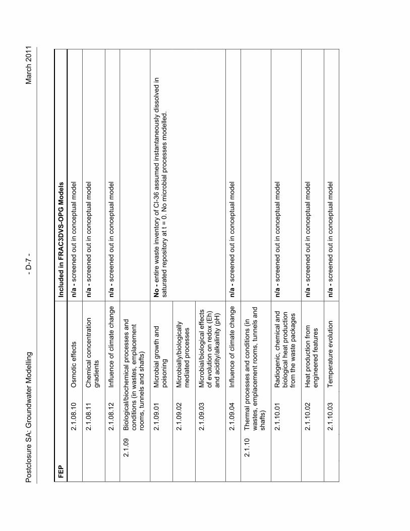
Pos
tclo
sure
SA
: Gro
und
wat
er M
odel
ling
- D
-7 -
M
arch
201
1
FE
P
In
clu
ded
in F
RA
C3D
VS
-OP
G M
od
els
2.1.
08.1
0 O
smot
ic e
ffect
s n
/a -
scr
eene
d ou
t in
conc
eptu
al m
odel
2.1.
08.1
1 C
hem
ical
con
cent
ratio
n gr
adie
nts
n/a
- s
cree
ned
out i
n co
ncep
tual
mod
el
2.1.
08.1
2
Influ
ence
of c
limat
e ch
ange
n
/a -
scr
eene
d ou
t in
conc
eptu
al m
odel
2.
1.09
B
iolo
gica
l/bio
chem
ical
pro
cess
es a
nd
cond
ition
s (in
was
tes,
em
plac
emen
t ro
oms,
tunn
els
and
shaf
ts)
2.1.
09.0
1
Mic
robi
al g
row
th a
nd
pois
onin
g N
o -
ent
ire w
aste
inve
ntor
y of
Cl-3
6 a
ssum
ed in
stan
tane
ousl
y di
ssol
ved
in
satu
rate
d re
posi
tory
at t
= 0
. No
mic
robi
al p
roce
sses
mod
elle
d.
2.
1.09
.02
M
icro
bial
ly/b
iolo
gica
lly
med
iate
d pr
oces
ses
2.
1.09
.03
Mic
robi
al/b
iolo
gica
l effe
cts
of e
volu
tion
on r
edox
(E
h)
and
acid
ity/a
lkal
inity
(pH
)
2.
1.09
.04
In
fluen
ce o
f clim
ate
chan
ge
n/a
- s
cree
ned
out i
n co
ncep
tual
mod
el
2.1.
10
The
rmal
pro
cess
es a
nd c
ondi
tions
(in
w
aste
s, e
mpl
acem
ent r
oom
s, tu
nnel
s an
d sh
afts
)
2.1.
10.0
1 R
adio
geni
c, c
hem
ical
and
bi
olog
ical
hea
t pro
duct
ion
from
the
was
te p
acka
ges
n/a
- s
cree
ned
out i
n co
ncep
tual
mod
el
2.1.
10.0
2 H
eat p
rodu
ctio
n fr
om
engi
neer
ed fe
atur
es
n/a
- s
cree
ned
out i
n co
ncep
tual
mod
el
2.1.
10.0
3
Tem
pera
ture
evo
lutio
n n
/a -
scr
eene
d ou
t in
conc
eptu
al m
odel
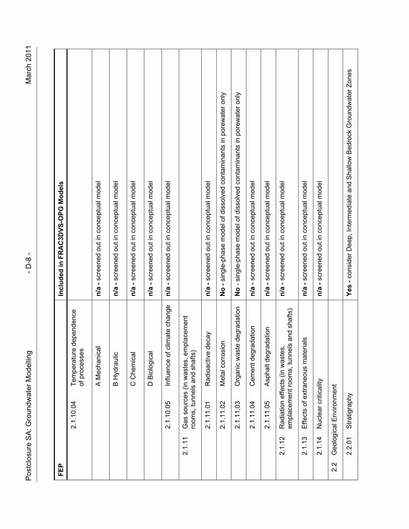
Pos
tclo
sure
SA
: Gro
und
wat
er M
odel
ling
- D
-8 -
M
arch
201
1
FE
P
In
clu
ded
in F
RA
C3D
VS
-OP
G M
od
els
2.1.
10.0
4 T
empe
ratu
re d
epen
denc
e of
pro
cess
es
A
Mec
hani
cal
n/a
- s
cree
ned
out i
n co
ncep
tual
mod
el
B
Hyd
raul
ic
n/a
- s
cree
ned
out i
n co
ncep
tual
mod
el
C
Che
mic
al
n/a
- s
cree
ned
out i
n co
ncep
tual
mod
el
D
Bio
logi
cal
n/a
- s
cree
ned
out i
n co
ncep
tual
mod
el
2.1.
10.0
5 In
fluen
ce o
f clim
ate
chan
ge
n/a
- s
cree
ned
out i
n co
ncep
tual
mod
el
2.
1.11
G
as s
ourc
es (
in w
aste
s, e
mpl
acem
ent
room
s, tu
nnel
s an
d sh
afts
)
2.1.
11.0
1 R
adio
activ
e de
cay
n/a
- s
cree
ned
out i
n co
ncep
tual
mod
el
2.1.
11.0
2 M
etal
cor
rosi
on
No
- s
ingl
e-ph
ase
mod
el o
f dis
solv
ed c
onta
min
ants
in p
orew
ater
onl
y
2.1.
11,0
3 O
rgan
ic w
aste
deg
rada
tion
No
- s
ingl
e-ph
ase
mod
el o
f dis
solv
ed c
onta
min
ants
in p
orew
ater
onl
y
2.1.
11.0
4 C
emen
t deg
rada
tion
n/a
- s
cree
ned
out i
n co
ncep
tual
mod
el
2.1.
11.0
5 A
spha
lt de
grad
atio
n n
/a -
scr
eene
d ou
t in
conc
eptu
al m
odel
2.
1.12
R
adia
tion
effe
cts
(in w
aste
s,
empl
acem
ent r
oom
s, tu
nnel
s an
d sh
afts
) n
/a -
scr
eene
d ou
t in
conc
eptu
al m
odel
2.
1.13
E
ffect
s of
ext
rane
ous
mat
eria
ls
n/a
- s
cree
ned
out i
n co
ncep
tual
mod
el
2.
1.14
N
ucle
ar c
ritic
ality
n
/a -
scr
eene
d ou
t in
conc
eptu
al m
odel
2.2
Geo
logi
cal E
nviro
nmen
t
2.
2.01
S
trat
igra
phy
Yes
- c
onsi
der
Dee
p, In
term
edia
te a
nd S
hallo
w B
edro
ck G
roun
dwat
er Z
ones
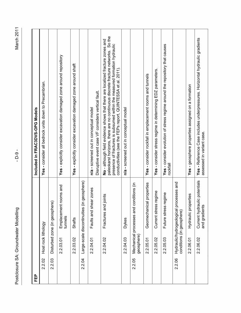
Pos
tclo
sure
SA
: Gro
und
wat
er M
odel
ling
- D
-9 -
M
arch
201
1
FE
P
In
clu
ded
in F
RA
C3D
VS
-OP
G M
od
els
2.
2.02
H
ost r
ock
litho
logy
Y
es -
con
side
r al
l bed
rock
uni
ts d
own
to P
reca
mbr
ian.
2.
2.03
D
istu
rbed
zon
e (in
geo
sphe
re)
2.2.
03.0
1 E
mpl
acem
ent r
oom
s an
d tu
nnel
s Y
es -
exp
licitl
y co
nsid
er e
xcav
atio
n da
mag
ed z
one
arou
nd r
epos
itory
2.2.
03.0
2 S
hafts
Y
es -
exp
licitl
y co
nsid
er e
xcav
atio
n da
mag
ed z
one
arou
nd s
haft
2.
2.04
La
rge-
scal
e di
scon
tinui
ties
(in g
eosp
here
)
2.2.
04.0
1 F
aults
and
she
ar z
ones
n
/a -
scr
eene
d ou
t in
conc
eptu
al m
odel
Dis
rupt
ive
even
t cas
e V
F c
onsi
ders
ver
tical
faul
t.
2.2.
04.0
2 F
ract
ures
and
join
ts
No
- a
lthou
gh fi
eld
evid
ence
sho
ws
that
ther
e ar
e lo
caliz
ed fr
actu
re z
ones
and
pa
leok
arst
hor
izon
s, th
ere
are
no c
ontin
uous
dis
cret
e fr
actu
re n
etw
orks
. S
o th
e pr
esen
ce o
f fra
ctur
es is
sub
sum
ed w
ithin
the
mea
sure
d fo
rmat
ion
hydr
aulic
co
nduc
tiviti
es (
see
the
FE
Ps
repo
rt, Q
UIN
TE
SS
A e
t al.
2011
).
2.2.
04.0
3 D
ykes
n
/a -
scr
eene
d ou
t in
conc
eptu
al m
odel
2.
2.05
M
echa
nica
l pro
cess
es a
nd c
ondi
tions
(in
ge
osph
ere)
2.2.
05.0
1 G
eom
echa
nica
l pro
pert
ies
Yes
- c
onsi
der
rock
fall
in e
mpl
acem
ent r
oom
s an
d tu
nnel
s
2.2.
05.0
2 C
urre
nt s
tres
s re
gim
e Y
es -
con
side
r st
ress
reg
ime
in d
eter
min
ing
ED
Z p
aram
eter
s.
2.2.
05.0
3 F
utur
e st
ress
reg
ime
Yes
- c
onsi
der
evol
utio
n of
str
ess
regi
me
aro
und
the
repo
sito
ry th
at c
ause
s ro
ckfa
ll
2.
2.06
H
ydra
ulic
/hyd
roge
olog
ical
pro
cess
es a
nd
cond
ition
s (in
geo
sphe
re)
2.2.
06.0
1 H
ydra
ulic
pro
pert
ies
Yes
- g
eosp
here
pro
pert
ies
assi
gned
on
a fo
rmat
ion
2.2.
06.0
2 C
urre
nt h
ydra
ulic
pot
entia
ls
and
grad
ient
s Y
es -
Ref
eren
ce C
ase
incl
udes
und
erpr
essu
res.
Hor
izon
tal h
ydra
ulic
gra
dien
ts
asse
ssed
in v
aria
nt c
ase.
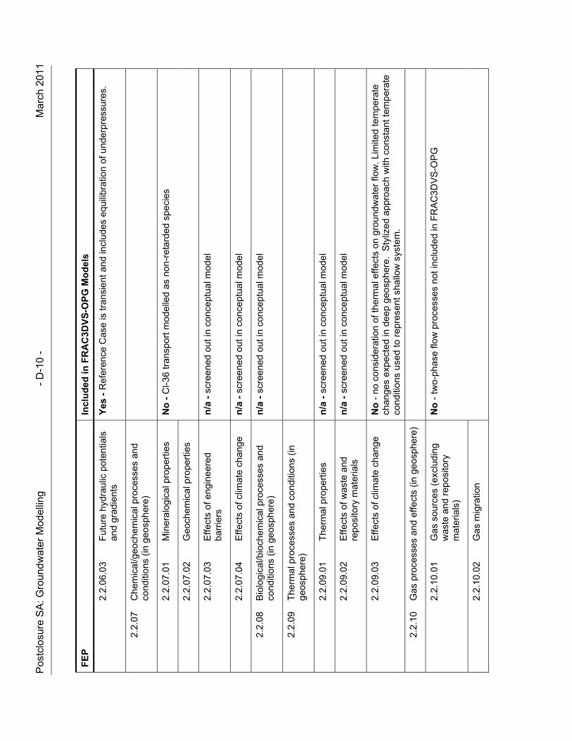
Pos
tclo
sure
SA
: Gro
und
wat
er M
odel
ling
- D
-10
- M
arch
201
1
FE
P
In
clu
ded
in F
RA
C3D
VS
-OP
G M
od
els
2.2.
06.0
3 F
utur
e hy
drau
lic p
oten
tials
an
d gr
adie
nts
Yes
- R
efer
ence
Cas
e is
tran
sien
t and
incl
udes
equ
ilibr
atio
n of
und
erpr
essu
res.
2.
2.07
C
hem
ical
/geo
chem
ical
pro
cess
es a
nd
cond
ition
s (in
geo
sphe
re)
2.2.
07.0
1 M
iner
alog
ical
pro
pert
ies
No
- C
l-36
tran
spor
t mod
elle
d as
non
-ret
arde
d sp
ecie
s
2.2.
07.0
2 G
eoch
emic
al p
rope
rtie
s
2.2.
07.0
3 E
ffect
s of
eng
inee
red
barr
iers
n
/a -
scr
eene
d ou
t in
conc
eptu
al m
odel
2.2.
07.0
4 E
ffect
s of
clim
ate
chan
ge
n/a
- s
cree
ned
out i
n co
ncep
tual
mod
el
2.
2.08
B
iolo
gica
l/bio
chem
ical
pro
cess
es a
nd
cond
ition
s (in
geo
sphe
re)
n/a
- s
cree
ned
out i
n co
ncep
tual
mod
el
2.
2.09
T
herm
al p
roce
sses
and
con
ditio
ns (
in
geos
pher
e)
2.2.
09.0
1 T
herm
al p
rope
rtie
s n
/a -
scr
eene
d ou
t in
conc
eptu
al m
odel
2.2.
09.0
2 E
ffect
s of
was
te a
nd
repo
sito
ry m
ater
ials
n
/a -
scr
eene
d ou
t in
conc
eptu
al m
odel
2.2.
09.0
3 E
ffect
s of
clim
ate
chan
ge
No
- n
o co
nsid
erat
ion
of th
erm
al e
ffect
s on
gro
undw
ater
flow
. Lim
ited
tem
pera
te
chan
ges
expe
cted
in d
eep
geos
pher
e. S
tyliz
ed a
ppro
ach
with
con
stan
t tem
pera
te
cond
ition
s us
ed to
rep
rese
nt s
hallo
w s
yste
m.
2.
2.10
G
as p
roce
sses
and
effe
cts
(in g
eosp
here
)
2.2.
10.0
1 G
as s
ourc
es (
excl
udin
g w
aste
and
rep
osito
ry
mat
eria
ls)
No
- tw
o-ph
ase
flow
pro
cess
es n
ot in
clud
ed in
FR
AC
3DV
S-O
PG
2.2.
10.0
2 G
as m
igra
tion
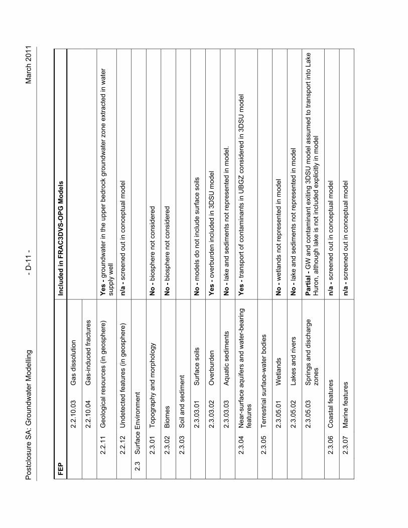
Pos
tclo
sure
SA
: Gro
und
wat
er M
odel
ling
- D
-11
- M
arch
201
1
FE
P
In
clu
ded
in F
RA
C3D
VS
-OP
G M
od
els
2.2.
10.0
3 G
as d
isso
lutio
n
2.2.
10.0
4 G
as-in
duce
d fr
actu
res
2.
2.11
G
eolo
gica
l res
ourc
es (
in g
eosp
here
) Y
es -
gro
undw
ater
in th
e up
per
bedr
ock
grou
ndw
ater
zon
e ex
trac
ted
in w
ater
su
pply
wel
l
2.
2.12
U
ndet
ecte
d fe
atur
es (
in g
eosp
here
) n
/a -
scr
eene
d ou
t in
conc
eptu
al m
odel
2.3
Sur
face
Env
ironm
ent
2.
3.01
T
opog
raph
y an
d m
orph
olog
y N
o -
bio
sphe
re n
ot c
onsi
dere
d
2.
3.02
B
iom
es
N
o -
bio
sphe
re n
ot c
onsi
dere
d
2.
3.03
S
oil a
nd s
edim
ent
2.3.
03.0
1 S
urfa
ce s
oils
N
o -
mod
els
do n
ot in
clud
e su
rfac
e so
ils
2.3.
03.0
2 O
verb
urde
n Y
es -
ove
rbur
den
incl
uded
in 3
DS
U m
odel
2.3.
03.0
3 A
quat
ic s
edim
ents
N
o -
lake
and
sed
imen
ts n
ot r
epre
sent
ed in
mod
el.
2.
3.04
N
ear-
surf
ace
aqui
fers
and
wat
er-b
earin
g fe
atur
es
Yes
- tr
ansp
ort o
f con
tam
inan
ts in
UB
GZ
con
side
red
in 3
DS
U m
odel
2.
3.05
T
erre
stria
l sur
face
-wat
er b
odie
s
2.3.
05.0
1 W
etla
nds
No
- w
etla
nds
not r
epre
sent
ed in
mod
el
2.3.
05.0
2 La
kes
and
river
s N
o -
lake
and
sed
imen
ts n
ot r
epre
sent
ed in
mod
el
2.3.
05.0
3 S
prin
gs a
nd d
isch
arge
zo
nes
Par
tial
- G
W a
nd c
onta
min
ant e
xitin
g 3D
SU
mod
el a
ssum
ed to
tran
spor
t int
o La
ke
Hur
on, a
lthou
gh la
ke is
not
incl
uded
exp
licitl
y in
mod
el
2.
3.06
C
oast
al fe
atur
es
n/a
- s
cree
ned
out i
n co
ncep
tual
mod
el
2.
3.07
M
arin
e fe
atur
es
n/a
- s
cree
ned
out i
n co
ncep
tual
mod
el
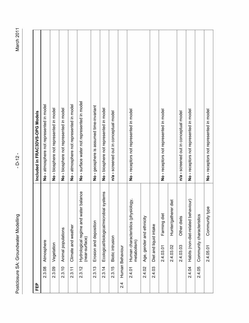
Pos
tclo
sure
SA
: Gro
und
wat
er M
odel
ling
- D
-12
- M
arch
201
1
FE
P
In
clu
ded
in F
RA
C3D
VS
-OP
G M
od
els
2.
3.08
A
tmos
pher
e N
o -
atm
osph
ere
not r
epre
sent
ed in
mod
el
2.
3.09
V
eget
atio
n
No
- b
iosp
here
not
rep
rese
nted
in m
odel
2.
3.10
A
nim
al p
opul
atio
ns
No
- b
iosp
here
not
rep
rese
nted
in m
odel
2.
3.11
C
limat
e an
d w
eath
er
No
- a
tmos
pher
e no
t rep
rese
nted
in m
odel
2.
3.12
H
ydro
logi
cal r
egim
e an
d w
ater
bal
ance
(n
ear-
surf
ace)
N
o -
sur
face
wat
er n
ot r
epre
sent
ed in
mod
el
2.3.
13
Ero
sion
and
dep
ositi
on
No
- g
eosp
here
is a
ssum
ed ti
me-
inva
riant
2.
3.14
E
colo
gica
l/bio
logi
cal/m
icro
bial
sys
tem
s N
o -
bio
sphe
re n
ot r
epre
sent
ed in
mod
el
2.
3.15
B
iotic
intr
usio
n n
/a -
scr
eene
d ou
t in
conc
eptu
al m
odel
2.4
Hum
an B
ehav
iour
2.
4.01
H
uman
cha
ract
eris
tics
(phy
siol
ogy,
m
etab
olis
m)
No
- r
ecep
tors
not
rep
rese
nted
in m
odel
2.
4.02
A
ge, g
ende
r an
d et
hnic
ity
2.4.
03
Die
t and
liqu
id in
take
2.
4.03
.01
Far
min
g di
et
No
- r
ecep
tors
not
rep
rese
nted
in m
odel
2.
4.03
.02
Hun
ter/
gath
erer
die
t
2.4.
03.0
3 O
ther
die
ts
n/a
- s
cree
ned
out i
n co
ncep
tual
mod
el
2.4.
04
Hab
its (
non-
diet
-rel
ated
beh
avio
ur)
No
- r
ecep
tors
not
rep
rese
nted
in m
odel
2.4.
05
Com
mun
ity c
hara
cter
istic
s
2.
4.05
.01
Com
mun
ity ty
pe
No
- r
ecep
tors
not
rep
rese
nted
in m
odel
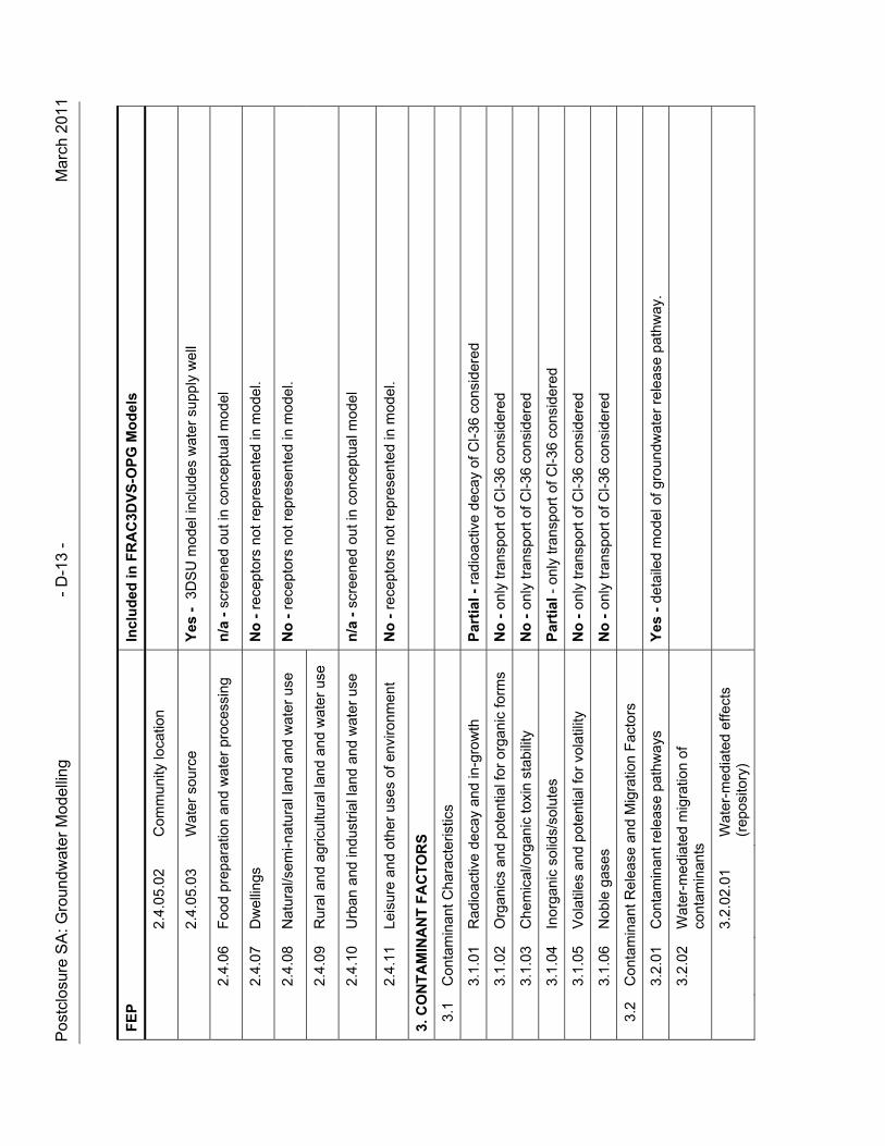
Pos
tclo
sure
SA
: Gro
und
wat
er M
odel
ling
- D
-13
- M
arch
201
1
FE
P
In
clu
ded
in F
RA
C3D
VS
-OP
G M
od
els
2.4.
05.0
2 C
omm
unity
loca
tion
2.
4.05
.03
Wat
er s
ourc
e Y
es -
3D
SU
mod
el in
clud
es w
ater
sup
ply
wel
l
2.
4.06
F
ood
prep
arat
ion
and
wat
er p
roce
ssin
g n
/a -
scr
eene
d ou
t in
conc
eptu
al m
odel
2.
4.07
D
wel
lings
No
- r
ecep
tors
not
rep
rese
nted
in m
odel
.
2.
4.08
N
atur
al/s
emi-n
atur
al la
nd a
nd w
ater
use
N
o -
rec
epto
rs n
ot r
epre
sent
ed in
mod
el.
2.
4.09
R
ural
and
agr
icul
tura
l lan
d an
d w
ater
use
2.
4.10
U
rban
and
indu
stria
l lan
d an
d w
ater
use
n
/a -
scr
eene
d ou
t in
conc
eptu
al m
odel
2.
4.11
Le
isur
e an
d ot
her
uses
of e
nviro
nmen
t N
o -
rec
epto
rs n
ot r
epre
sent
ed in
mod
el.
3. C
ON
TA
MIN
AN
T F
AC
TO
RS
3.1
Con
tam
inan
t Cha
ract
eris
tics
3.
1.01
R
adio
activ
e de
cay
and
in-g
row
th
Par
tial
- r
adio
activ
e de
cay
of C
l-36
cons
ider
ed
3.
1.02
O
rgan
ics
and
pote
ntia
l for
org
anic
form
s N
o -
onl
y tr
ansp
ort o
f Cl-3
6 co
nsid
ered
3.
1.03
C
hem
ical
/org
anic
toxi
n st
abili
ty
No
- o
nly
tran
spor
t of C
l-36
cons
ider
ed
3.
1.04
In
orga
nic
solid
s/so
lute
s P
arti
al -
onl
y tr
ansp
ort o
f Cl-3
6 co
nsid
ered
3.1.
05
Vol
atile
s an
d po
tent
ial f
or v
olat
ility
N
o -
onl
y tr
ansp
ort o
f Cl-3
6 co
nsid
ered
3.
1.06
N
oble
gas
es
No
- o
nly
tran
spor
t of C
l-36
cons
ider
ed
3.2
Con
tam
inan
t Rel
ease
and
Mig
ratio
n F
acto
rs
3.
2.01
C
onta
min
ant r
elea
se p
athw
ays
Yes
- d
etai
led
mod
el o
f gro
undw
ater
rel
ease
pat
hway
.
3.
2.02
W
ater
-med
iate
d m
igra
tion
of
cont
amin
ants
3.2.
02.0
1 W
ater
-med
iate
d ef
fect
s (r
epos
itory
)
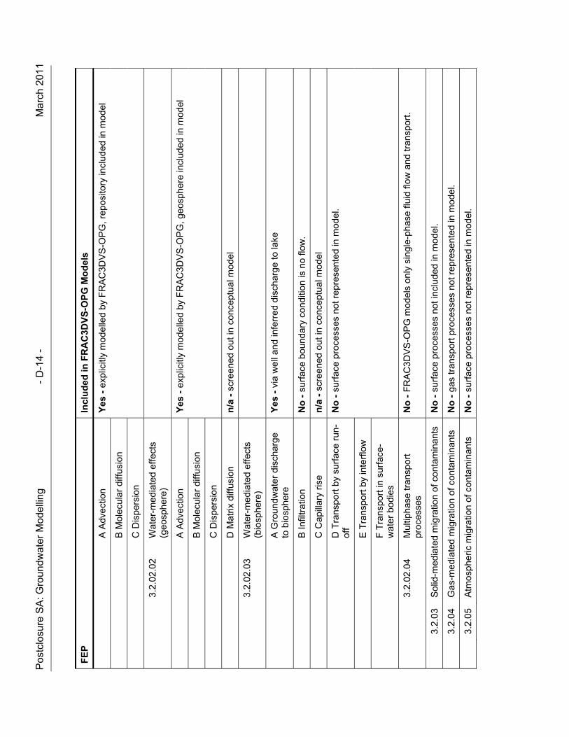
Pos
tclo
sure
SA
: Gro
und
wat
er M
odel
ling
- D
-14
- M
arch
201
1
FE
P
In
clu
ded
in F
RA
C3D
VS
-OP
G M
od
els
A
Adv
ectio
n Y
es -
exp
licitl
y m
odel
led
by F
RA
C3D
VS
-OP
G, r
epos
itory
incl
uded
in m
odel
B
Mol
ecul
ar d
iffus
ion
C
Dis
per
sio
n
3.2.
02.0
2 W
ater
-med
iate
d ef
fect
s (g
eosp
here
)
A
Adv
ectio
n Y
es -
exp
licitl
y m
odel
led
by F
RA
C3D
VS
-OP
G, g
eosp
here
incl
uded
in m
odel
B
Mol
ecul
ar d
iffus
ion
C
Dis
per
sio
n
D
Mat
rix d
iffus
ion
n/a
- s
cree
ned
out i
n co
ncep
tual
mod
el
3.2.
02.0
3 W
ater
-med
iate
d ef
fect
s (b
iosp
here
)
A
Gro
undw
ater
dis
char
ge
to b
iosp
here
Y
es -
via
wel
l and
infe
rred
dis
char
ge to
lake
B
Infil
trat
ion
No
- s
urfa
ce b
ound
ary
cond
ition
is n
o flo
w.
C
Cap
illar
y ris
e n
/a -
scr
eene
d ou
t in
conc
eptu
al m
odel
D
Tra
nspo
rt b
y su
rfac
e ru
n-of
f N
o -
sur
face
pro
cess
es n
ot r
epre
sent
ed in
mod
el.
E
Tra
nspo
rt b
y in
terf
low
F
Tra
nspo
rt in
sur
face
-w
ater
bod
ies
3.2.
02.0
4 M
ultip
hase
tran
spor
t pr
oces
ses
No
- F
RA
C3D
VS
-OP
G m
odel
s on
ly s
ingl
e-ph
ase
fluid
flow
and
tran
spor
t.
3.
2.03
S
olid
-med
iate
d m
igra
tion
of c
onta
min
ants
N
o -
sur
face
pro
cess
es n
ot in
clud
ed in
mod
el.
3.
2.04
G
as-m
edia
ted
mig
ratio
n of
con
tam
inan
ts
No
- g
as tr
ansp
ort p
roce
sses
not
rep
rese
nted
in m
odel
.
3.
2.05
A
tmos
pher
ic m
igra
tion
of c
onta
min
ants
N
o -
sur
face
pro
cess
es n
ot r
epre
sent
ed in
mod
el.
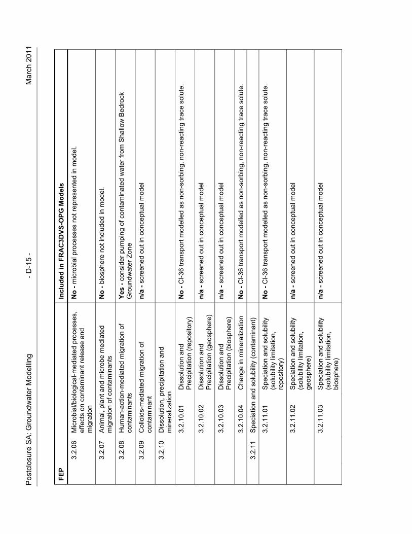
Pos
tclo
sure
SA
: Gro
und
wat
er M
odel
ling
- D
-15
- M
arch
201
1
FE
P
In
clu
ded
in F
RA
C3D
VS
-OP
G M
od
els
3.
2.06
M
icro
bial
/bio
logi
cal-m
edia
ted
proc
esse
s,
effe
cts
on c
onta
min
ant r
elea
se a
nd
mig
ratio
n
No
- m
icro
bial
pro
cess
es n
ot r
epre
sent
ed in
mod
el.
3.
2.07
A
nim
al, p
lant
and
mic
robe
med
iate
d m
igra
tion
of c
onta
min
ants
N
o -
bio
sphe
re n
ot in
clud
ed in
mod
el.
3.
2.08
H
uman
-act
ion-
med
iate
d m
igra
tion
of
cont
amin
ants
Y
es -
con
side
r pu
mpi
ng o
f con
tam
inat
ed w
ater
from
Sha
llow
Bed
rock
G
roun
dwat
er Z
one
3.
2.09
C
ollo
ids-
med
iate
d m
igra
tion
of
cont
amin
ant
n/a
- s
cree
ned
out i
n co
ncep
tual
mod
el
3.
2.10
D
isso
lutio
n, p
reci
pita
tion
and
min
eral
izat
ion
3.2.
10.0
1 D
isso
lutio
n an
d P
reci
pita
tion
(rep
osito
ry)
No
- C
l-36
tran
spor
t mod
elle
d as
non
-sor
bing
, non
-rea
ctin
g tr
ace
solu
te.
3.2.
10.0
2 D
isso
lutio
n an
d P
reci
pita
tion
(geo
sphe
re)
n/a
- s
cree
ned
out i
n co
ncep
tual
mod
el
3.2.
10.0
3 D
isso
lutio
n an
d P
reci
pita
tion
(bio
sphe
re)
n/a
- s
cree
ned
out i
n co
ncep
tual
mod
el
3.2.
10.0
4 C
hang
e in
min
eral
izat
ion
No
- C
l-36
tran
spor
t mod
elle
d as
non
-sor
bing
, non
-rea
ctin
g tr
ace
solu
te.
3.
2.11
S
peci
atio
n an
d so
lubi
lity
(con
tam
inan
t)
3.2.
11.0
1 S
peci
atio
n an
d so
lubi
lity
(sol
ubili
ty li
mita
tion,
re
posi
tory
)
No
- C
l-36
tran
spor
t mod
elle
d as
non
-sor
bing
, non
-rea
ctin
g tr
ace
solu
te.
3.2.
11.0
2 S
peci
atio
n an
d so
lubi
lity
(sol
ubili
ty li
mita
tion,
ge
osph
ere)
n/a
- s
cree
ned
out i
n co
ncep
tual
mod
el
3.2.
11.0
3 S
peci
atio
n an
d so
lubi
lity
(sol
ubili
ty li
mita
tion,
bi
osph
ere)
n/a
- s
cree
ned
out i
n co
ncep
tual
mod
el
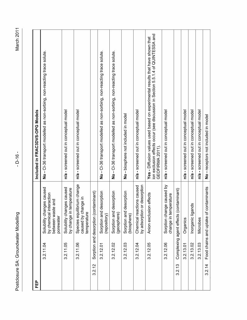
Pos
tclo
sure
SA
: Gro
und
wat
er M
odel
ling
- D
-16
- M
arch
201
1
FE
P
In
clu
ded
in F
RA
C3D
VS
-OP
G M
od
els
3.2.
11.0
4 S
olub
ility
cha
nges
cau
sed
by c
hem
ical
inte
ract
ion
betw
een
was
te a
nd
pore
wat
er
No
- C
l-36
tran
spor
t mod
elle
d as
non
-sor
bing
, non
-rea
ctin
g tr
ace
solu
te.
3.
2.11
.05
Sol
ubili
ty c
hang
es c
ause
d by
cha
nge
in te
mpe
ratu
re
n/a
- s
cree
ned
out i
n co
ncep
tual
mod
el
3.2.
11.0
6 S
peci
es e
quili
briu
m c
hang
e ca
used
by
chan
ge in
te
mpe
ratu
re
n/a
- s
cree
ned
out i
n co
ncep
tual
mod
el
3.
2.12
S
orpt
ion
and
deso
rptio
n (c
onta
min
ant)
3.2.
12.0
1 S
orpt
ion
and
deso
rptio
n (r
epos
itory
) N
o -
Cl-3
6 tr
ansp
ort m
odel
led
as n
on-s
orbi
ng, n
on-r
eact
ing
trac
e so
lute
.
3.2.
12.0
2 S
orpt
ion
and
deso
rptio
n (g
eosp
here
) N
o -
Cl-3
6 tr
ansp
ort m
odel
led
as n
on-s
orbi
ng, n
on-r
eact
ing
trac
e so
lute
.
3.2.
12.0
3 S
orpt
ion
and
deso
rptio
n (b
iosp
here
) N
o -
bio
sphe
re n
ot in
clud
ed in
mod
el
3.2.
12.0
4 C
hem
ical
rea
ctio
ns c
ause
d by
ads
orpt
ion
or d
esor
ptio
n n
/a -
scr
eene
d ou
t in
conc
eptu
al m
odel
3.2.
12.0
5 A
nion
exc
lusi
on e
ffect
s Y
es -
Diff
usio
n va
lues
use
d ba
sed
on e
xper
imen
tal r
esul
ts th
at h
ave
show
n th
at
ion
excl
usio
n ef
fect
s oc
cur
(see
dis
cuss
ion
in S
ectio
n 5.
5.1.
4 of
QU
INT
ES
SA
and
G
EO
FIR
MA
201
1).
3.2.
12.0
6 S
orpt
ion
chan
ge c
ause
d by
ch
ange
in te
mpe
ratu
re
n/a
- s
cree
ned
out i
n co
ncep
tual
mod
el
3.
2.13
C
ompl
exin
g ag
ent e
ffect
s (c
onta
min
ant)
3.2.
13.0
1 O
rgan
ics
n/a
- s
cree
ned
out i
n co
ncep
tual
mod
el
3.2.
13.0
2 In
orga
nic
ligan
ds
n/a
- s
cree
ned
out i
n co
ncep
tual
mod
el
3.2.
13.0
3 M
icro
bes
n/a
- s
cree
ned
out i
n co
ncep
tual
mod
el
3.
2.14
F
ood
chai
ns a
nd u
ptak
e of
con
tam
inan
ts
No
- r
ecep
tors
not
incl
uded
in m
odel
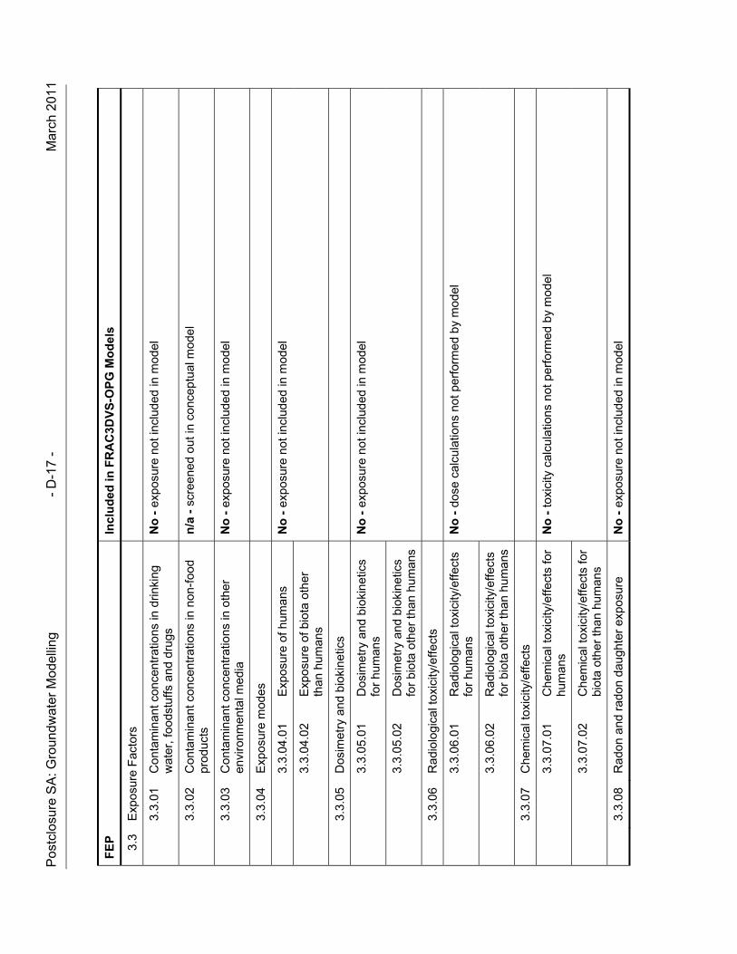
Pos
tclo
sure
SA
: Gro
und
wat
er M
odel
ling
- D
-17
- M
arch
201
1
FE
P
In
clu
ded
in F
RA
C3D
VS
-OP
G M
od
els
3.3
Exp
osur
e F
acto
rs
3.
3.01
C
onta
min
ant c
once
ntra
tions
in d
rinki
ng
wat
er, f
oods
tuffs
and
dru
gs
No
- e
xpos
ure
not i
nclu
ded
in m
odel
3.
3.02
C
onta
min
ant c
once
ntra
tions
in n
on-f
ood
prod
ucts
n
/a -
scr
eene
d ou
t in
conc
eptu
al m
odel
3.
3.03
C
onta
min
ant c
once
ntra
tions
in o
ther
en
viro
nmen
tal m
edia
N
o -
exp
osur
e no
t inc
lude
d in
mod
el
3.
3.04
E
xpos
ure
mod
es
3.3.
04.0
1 E
xpos
ure
of h
uman
s N
o -
exp
osur
e no
t inc
lude
d in
mod
el
3.3.
04.0
2 E
xpos
ure
of b
iota
oth
er
than
hum
ans
3.
3.05
D
osim
etry
and
bio
kine
tics
3.3.
05.0
1 D
osim
etry
and
bio
kine
tics
fo
r hu
man
s N
o -
exp
osur
e no
t inc
lude
d in
mod
el
3.3.
05.0
2 D
osim
etry
and
bio
kine
tics
fo
r bi
ota
othe
r th
an h
uman
s
3.
3.06
R
adio
logi
cal t
oxic
ity/e
ffect
s
3.3.
06.0
1 R
adio
logi
cal t
oxic
ity/e
ffect
s fo
r hu
man
s N
o -
dos
e ca
lcul
atio
ns n
ot p
erfo
rmed
by
mod
el
3.3.
06.0
2 R
adio
logi
cal t
oxic
ity/e
ffect
s fo
r bi
ota
othe
r th
an h
uman
s
3.
3.07
C
hem
ical
toxi
city
/effe
cts
3.3.
07.0
1 C
hem
ical
toxi
city
/effe
cts
for
hum
ans
No
- to
xici
ty c
alcu
latio
ns n
ot p
erfo
rmed
by
mod
el
3.3.
07.0
2 C
hem
ical
toxi
city
/effe
cts
for
biot
a ot
her
than
hum
ans
3.
3.08
R
adon
and
rad
on d
augh
ter
expo
sure
N
o -
exp
osur
e no
t inc
lude
d in
mod
el
Postclosure SA: Groundwater Modelling - D-18 - March 2011
REFERENCES FOR APPENDIX D
QUINTESSA. 2011. Postclosure Safety Assessment: System and Its Evolution. Quintessa Ltd. report for the Nuclear Waste Management Organization NWMO DGR-TR-2011-28 R000. Toronto, Canada.
QUINTESSA and GEOFIRMA. 2011. Postclosure Safety Assessment: Data. Quintessa Ltd. and Geofirma Engineering Ltd. report for the Nuclear Waste Management Organization NWMO DGR-TR-2011-32 R000. Toronto, Canada.
QUINTESSA, SENES and GEOFIRMA. 2011. Postclosure Safety Assessment: Features, Events and Processes. Quintessa Ltd., SENES Consultants Ltd. and Geofirma Engineering Ltd. report for the Nuclear Waste Management Organization NWMO DGR-TR-2011-29 R000. Toronto, Canada.
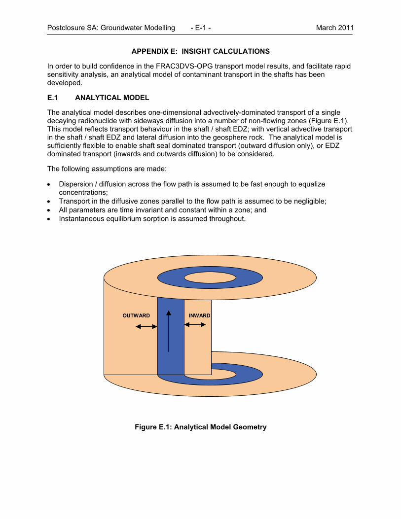
Postclosure SA: Groundwater Modelling - E-1 - March 2011
APPENDIX E: INSIGHT CALCULATIONS
In order to build confidence in the FRAC3DVS-OPG transport model results, and facilitate rapid sensitivity analysis, an analytical model of contaminant transport in the shafts has been developed.
E.1 ANALYTICAL MODEL
The analytical model describes one-dimensional advectively-dominated transport of a single decaying radionuclide with sideways diffusion into a number of non-flowing zones (Figure E.1). This model reflects transport behaviour in the shaft / shaft EDZ; with vertical advective transport in the shaft / shaft EDZ and lateral diffusion into the geosphere rock. The analytical model is sufficiently flexible to enable shaft seal dominated transport (outward diffusion only), or EDZ dominated transport (inwards and outwards diffusion) to be considered.
The following assumptions are made:
Dispersion / diffusion across the flow path is assumed to be fast enough to equalize concentrations;
Transport in the diffusive zones parallel to the flow path is assumed to be negligible; All parameters are time invariant and constant within a zone; and Instantaneous equilibrium sorption is assumed throughout.
INWARD OUTWARD
Figure E.1: Analytical Model Geometry
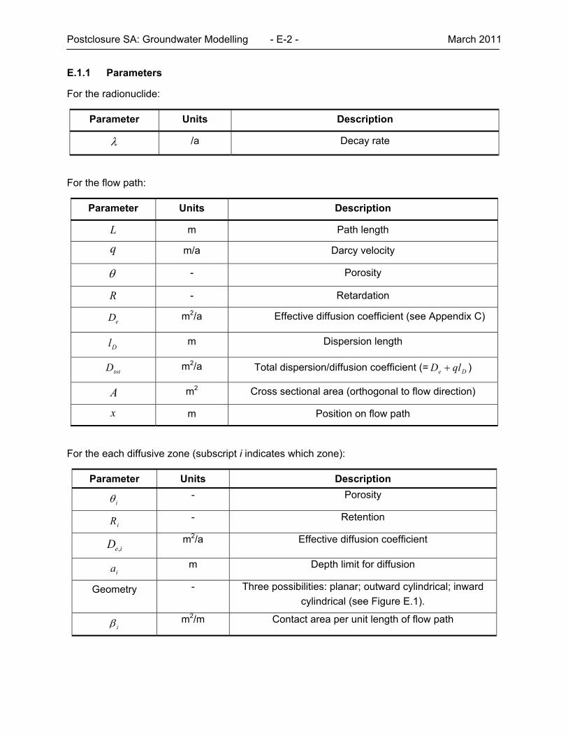
Postclosure SA: Groundwater Modelling - E-2 - March 2011
E.1.1 Parameters
For the radionuclide:
Parameter Units Description
/a Decay rate
For the flow path:
Parameter Units Description
L m Path length
q m/a Darcy velocity
- Porosity
R - Retardation
eD m2/a Effective diffusion coefficient (see Appendix C)
Dl m Dispersion length
totD m2/a Total dispersion/diffusion coefficient (= De qlD )
A m2 Cross sectional area (orthogonal to flow direction)
x m Position on flow path
For the each diffusive zone (subscript i indicates which zone):
Parameter Units Description
i - Porosity
iR - Retention
ieD , m2/a Effective diffusion coefficient
ia m Depth limit for diffusion
Geometry - Three possibilities: planar; outward cylindrical; inward
cylindrical (see Figure E.1).
i m2/m Contact area per unit length of flow path
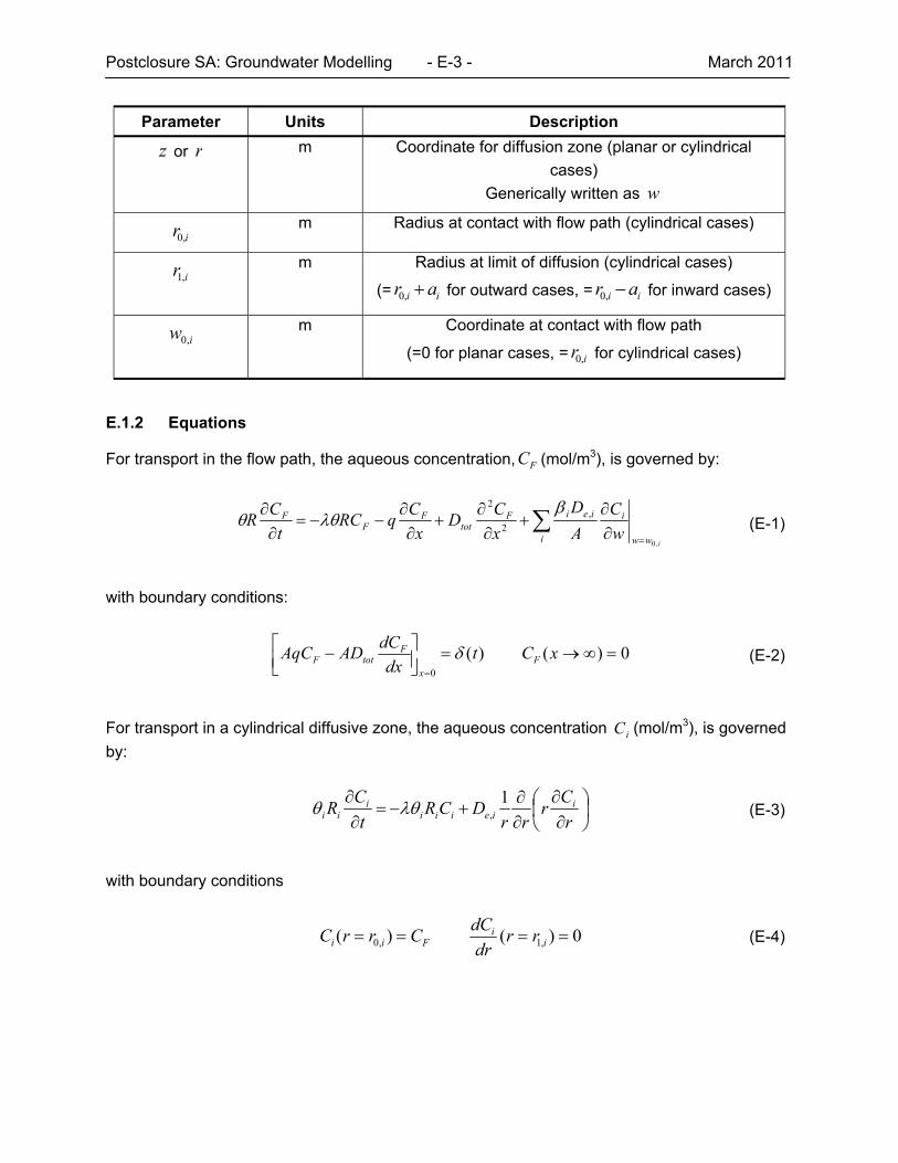
Postclosure SA: Groundwater Modelling - E-3 - March 2011
Parameter Units Description
z or r m Coordinate for diffusion zone (planar or cylindrical
cases)
Generically written as w
ir ,0 m Radius at contact with flow path (cylindrical cases)
ir ,1 m Radius at limit of diffusion (cylindrical cases)
(= ii ar ,0 for outward cases, = ii ar ,0 for inward cases)
iw ,0 m Coordinate at contact with flow path
(=0 for planar cases, = ir ,0 for cylindrical cases)
E.1.2 Equations
For transport in the flow path, the aqueous concentration, FC (mol/m3), is governed by:
iwwi
iieiFtot
FF
F
w
C
A
D
x
CD
x
CqRC
t
CR
,0
,
2
2
(E-1)
with boundary conditions:
0)()(0
xCtdx
dCADAqC F
x
FtotF (E-2)
For transport in a cylindrical diffusive zone, the aqueous concentration iC (mol/m3), is governed
by:
r
Cr
rrDCR
t
CR i
ieiiii
ii
1, (E-3)
with boundary conditions
0)()( ,1,0 ii
Fii rrdr
dCCrrC (E-4)
Postclosure SA: Groundwater Modelling - E-4 - March 2011
E.1.3 Laplace Transform Solutions
The solutions are easily derived. We start with the diffusive zones. An overbar denotes the Laplace transform throughout and s (/a) is the Laplace variable.
It is useful to define:
ie
iii D
sR
,
)(
(E-5)
For the cylindrical system,
)()()()(
)()()()(
,11,00,11,00
,110,110
iiiiiiii
iiiiiiFi rKrIrIrK
rKrIrIrKCC
(E-6)
and the matrix response function is given by
)()()()(
)()()()(
,11,00,11,00
,11,01,11,01
iiiiiiii
iiiiiiiiii rKrIrIrK
rKrIrIrKM
(E-7)
where the positive sign is for the outward cylinder (where the r coordinate increases away from the interface) and the negative sign is for the inward cylinder (where the r coordinate decreases away from the interface). Then, we can transform the flow path equation and rewrite it as an equation for the flux, F (mol/a).
Writing
)()()( , sMA
DsRsg
ii
iei
(E-8)
we obtain
xseF )( (E-9)
where
1
)(41
2)(
2q
sgD
D
qs tot
tot
(E-10)
Postclosure SA: Groundwater Modelling - E-5 - March 2011
E.1.4 Time Series Output
A code has been written to invert the Laplace transform solution back to the time domain. The code uses established algorithms based on Talbot (1979). The code outputs the contaminant concentration at the end of the flow path compared with the source (i.e., C/Co), with time.
The code has been verified by:
Comparison with solution of the analytical model for the fraction of contamination surviving transport, average arrival time and variance of the arrival time (calculated using a spreadsheet and by also by quadrature of the time series results); and
Comparison of time series results against Nagra’s transport code PICNIC.
E.2 APPLICATION
The analytical model was compared against FRAC3DVS-OPG for the simplified base case (NE-SBC) for a metric location in the shaft at the top of the Ordovician. The NE-SBC case was chosen because of the time invariance of the flows, and the monotonically upwards-directed flow in the shaft. The Reference Case was not selected for this analysis because of the transient nature of the flows and fact that shaft flows terminate in the underpressured Ordovician sediments over the 1 Ma performance period, which could not be accounted for in the analytical model. The metric location at the top of the Ordovician was chosen because the analytical model could not consider lateral advective transport into the Guelph and Salina A1 Upper Carbonate formations.
The flow path considered in this exercise included the access tunnel connecting repository Panel 1 to the monolith, the monolith and surrounding HDZ (see Figure E.2), , and the shaft seal materials from the repository horizon to the top of the Ordovician. Considering that the NE-SBC flow results indicate that the majority of the flow takes place in the shaft seal materials and not in the shaft EDZ, the analytical model was set-up to consider transport along this flow path with outwards diffusion only. Inwards diffusion was not considered.
This exercise required the selection of a single Darcy velocity applicable to the entire flow path, including the part within the open access tunnels (approximately 47 m, see Figure E.2), the part within the HDZ surrounding the concrete monolith (approximately 104 m, see Figure E.2) and the part within the shaft (including parts within bentonite/sand, concrete, and asphalt). A length weighted harmonic mean of Darcy velocities from the NE-SBC results were used for this purpose.
This exercise also required the selection of a single effective diffusion coefficient for the flow path and for the undisturbed rock. Length weighted harmonic means were used for this purpose.
Transport of Cl-36 was considered, consistent with the NE-SBC results. A continuous source was implemented as a reasonable approximation of the slowly decreasing repository concentrations determined in the NE-SBC case.
E.3 DATA
Data for the analytical model are described in Table E.1.
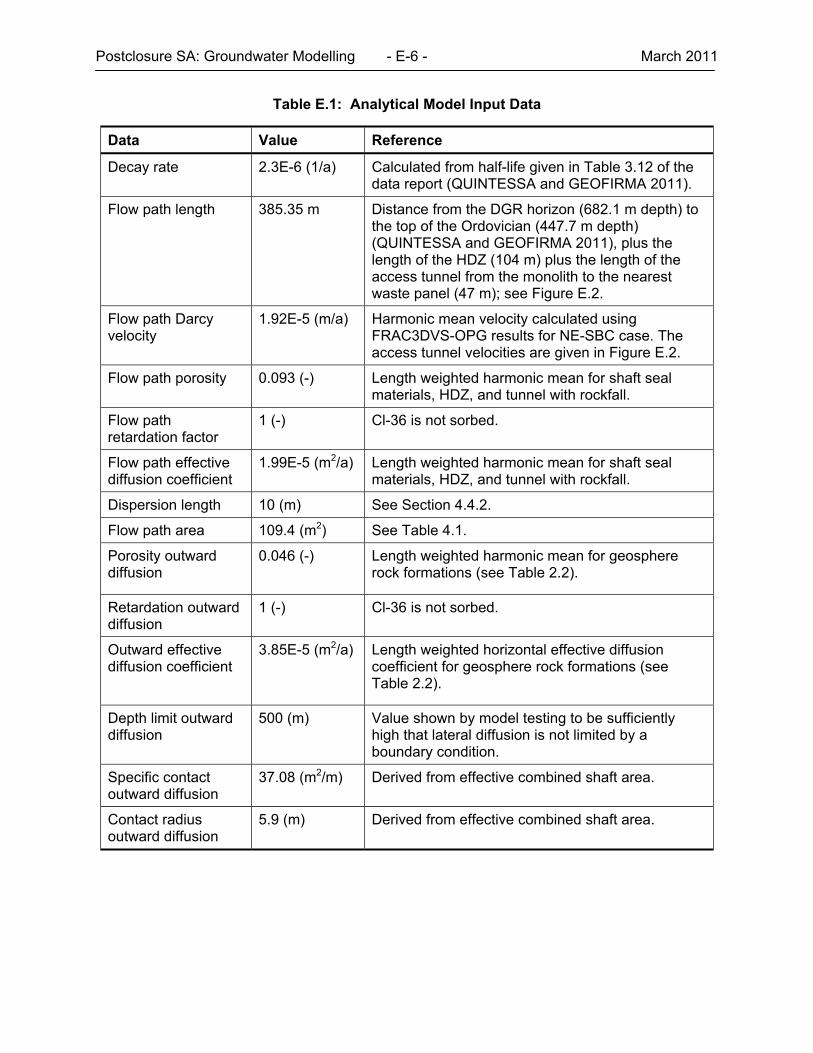
Postclosure SA: Groundwater Modelling - E-6 - March 2011
Table E.1: Analytical Model Input Data
Data Value Reference
Decay rate 2.3E-6 (1/a) Calculated from half-life given in Table 3.12 of the data report (QUINTESSA and GEOFIRMA 2011).
Flow path length 385.35 m Distance from the DGR horizon (682.1 m depth) to the top of the Ordovician (447.7 m depth) (QUINTESSA and GEOFIRMA 2011), plus the length of the HDZ (104 m) plus the length of the access tunnel from the monolith to the nearest waste panel (47 m); see Figure E.2.
Flow path Darcy velocity
1.92E-5 (m/a) Harmonic mean velocity calculated using FRAC3DVS-OPG results for NE-SBC case. The access tunnel velocities are given in Figure E.2.
Flow path porosity 0.093 (-) Length weighted harmonic mean for shaft seal materials, HDZ, and tunnel with rockfall.
Flow path retardation factor
1 (-) Cl-36 is not sorbed.
Flow path effective diffusion coefficient
1.99E-5 (m2/a) Length weighted harmonic mean for shaft seal materials, HDZ, and tunnel with rockfall.
Dispersion length 10 (m) See Section 4.4.2.
Flow path area 109.4 (m2) See Table 4.1.
Porosity outward diffusion
0.046 (-) Length weighted harmonic mean for geosphere rock formations (see Table 2.2).
Retardation outward diffusion
1 (-) Cl-36 is not sorbed.
Outward effective diffusion coefficient
3.85E-5 (m2/a) Length weighted horizontal effective diffusion coefficient for geosphere rock formations (see Table 2.2).
Depth limit outward diffusion
500 (m) Value shown by model testing to be sufficiently high that lateral diffusion is not limited by a boundary condition.
Specific contact outward diffusion
37.08 (m2/m) Derived from effective combined shaft area.
Contact radius outward diffusion
5.9 (m) Derived from effective combined shaft area.
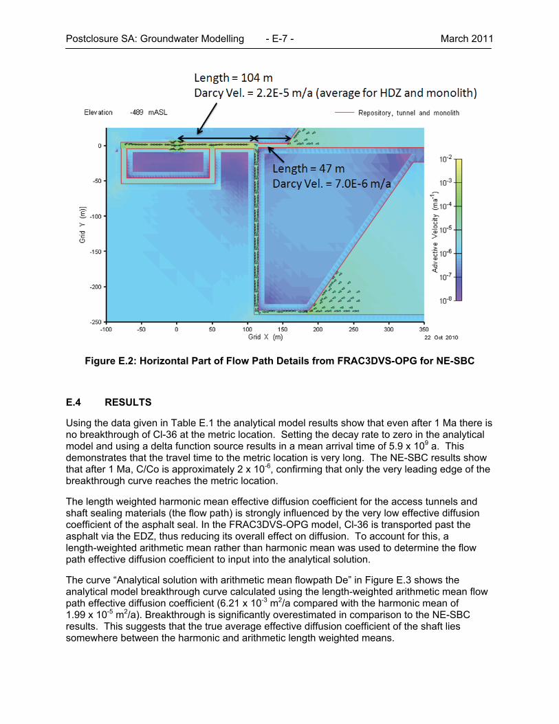
Postclosure SA: Groundwater Modelling - E-7 - March 2011
Figure E.2: Horizontal Part of Flow Path Details from FRAC3DVS-OPG for NE-SBC
E.4 RESULTS
Using the data given in Table E.1 the analytical model results show that even after 1 Ma there is no breakthrough of Cl-36 at the metric location. Setting the decay rate to zero in the analytical model and using a delta function source results in a mean arrival time of 5.9 x 10⁹ a. This demonstrates that the travel time to the metric location is very long. The NE-SBC results show that after 1 Ma, C/Co is approximately 2 x 10⁻⁶, confirming that only the very leading edge of the breakthrough curve reaches the metric location.
The length weighted harmonic mean effective diffusion coefficient for the access tunnels and shaft sealing materials (the flow path) is strongly influenced by the very low effective diffusion coefficient of the asphalt seal. In the FRAC3DVS-OPG model, Cl-36 is transported past the asphalt via the EDZ, thus reducing its overall effect on diffusion. To account for this, a length-weighted arithmetic mean rather than harmonic mean was used to determine the flow path effective diffusion coefficient to input into the analytical solution.
The curve “Analytical solution with arithmetic mean flowpath De” in Figure E.3 shows the analytical model breakthrough curve calculated using the length-weighted arithmetic mean flow path effective diffusion coefficient (6.21 x 10⁻³ m2/a compared with the harmonic mean of 1.99 x 10⁻⁵ m2/a). Breakthrough is significantly overestimated in comparison to the NE-SBC results. This suggests that the true average effective diffusion coefficient of the shaft lies somewhere between the harmonic and arithmetic length weighted means.
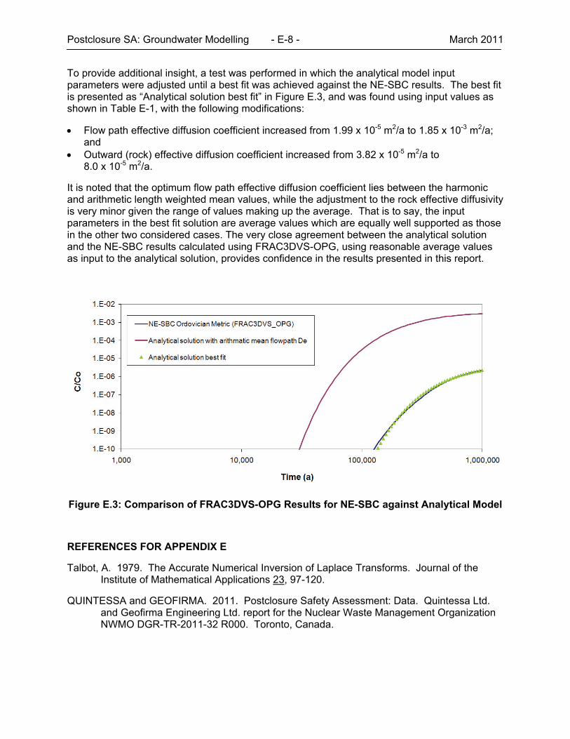
Postclosure SA: Groundwater Modelling - E-8 - March 2011
To provide additional insight, a test was performed in which the analytical model input parameters were adjusted until a best fit was achieved against the NE-SBC results. The best fit is presented as “Analytical solution best fit” in Figure E.3, and was found using input values as shown in Table E-1, with the following modifications:
Flow path effective diffusion coefficient increased from 1.99 x 10⁻⁵ m2/a to 1.85 x 10⁻³ m2/a; and
Outward (rock) effective diffusion coefficient increased from 3.82 x 10⁻⁵ m2/a to 8.0 x 10⁻⁵ m2/a.
It is noted that the optimum flow path effective diffusion coefficient lies between the harmonic and arithmetic length weighted mean values, while the adjustment to the rock effective diffusivity is very minor given the range of values making up the average. That is to say, the input parameters in the best fit solution are average values which are equally well supported as those in the other two considered cases. The very close agreement between the analytical solution and the NE-SBC results calculated using FRAC3DVS-OPG, using reasonable average values as input to the analytical solution, provides confidence in the results presented in this report.
Figure E.3: Comparison of FRAC3DVS-OPG Results for NE-SBC against Analytical Model
REFERENCES FOR APPENDIX E
Talbot, A. 1979. The Accurate Numerical Inversion of Laplace Transforms. Journal of the Institute of Mathematical Applications 23, 97-120.
QUINTESSA and GEOFIRMA. 2011. Postclosure Safety Assessment: Data. Quintessa Ltd. and Geofirma Engineering Ltd. report for the Nuclear Waste Management Organization NWMO DGR-TR-2011-32 R000. Toronto, Canada.