WASHINGTON UNIVERSITY IN ST. LOUIS

School of Engineering and Applied Science

Department of Mechanical, Aerospace, and Structural Engineering

Thesis Examination Committee:

Philip Bayly, Chair

Larry Taber

Susan Dutcher

MATHEMATICAL MODELS OF THE MECHANICS AND CONTROL OF CILIA

AND FLAGELLA

by

Kate E. Nevin

A thesis presented to the School of Engineering

of Washington University in partial fulfillment of the

requirements for the degree of

MASTER OF SCIENCE

May 2009

Saint Louis, Missouri

ii

ABSTRACT

Mathematical Models of the Mechanics and Control of Cilia and Flagella

by

Kate E. Nevin

Master of Science in Mechanical Engineering

Washington University in St. Louis, 2009

Research Advisor: Professor Philip Bayly

Cilia and flagella are thin hair-like organelles that protrude from various cell types.

Genetic mutations that affect the structure and motion of these organelles can have

severe consequences. In this thesis, mathematical models of the basic ciliary and

flagellar structure (the "axoneme") are reprised or developed anew to illuminate the

mechanical-chemical interactions that produce motion. These models focus on the

interactions between the motor protein dynein and passive structural elements.

Equations of motion are derived based on free body diagrams. In the first model (due to

Hines and Blum, 1978), dynein activity is assumed to depend on curvature. While this

model exhibits sustained oscillations, key features of flagellar waveforms are not

reproduced, and the proposed relationship between dynein activity and curvature is

unsupported by any biophysical argument. In the second model (due to Lindemann,

1994), dynein activity is hypothesized to depend mainly on doublet spacing, which is

driven by internal forces transverse to the longitudinal axis of the axoneme. This model

iii

produces realistic bending of the cilium, and the explanation of dynein switching is

detailed and plausible. However, the mechanical aspects of the model appear flawed,

and Lindemann's numerical methods are suspect. The third and fourth models

discussed in this thesis were developed during the course of the present study, and

consist of systems of partial differential equations (PDEs). The third model combines

the mechanical model of Hines and Blum (1978) with the switching mechanism of

Lindemann (1994). The model produces oscillations, but not the patterns of

propagating curvature that characterize real flagella. In the fourth model, dynein arm

adhesion is modeled as an "excitable" system, in which activity increases after a

threshold level is reached. This model reproduces the motion of the cilium much better

than the third model. The finite element program COMSOL is used to implement the

PDE models, and MATLAB post-processing routines are used to view the motion of the

organelle. The four models discussed in this thesis provide a theoretical framework in

which to formulate questions and hypotheses concerning ciliary and flagellar motion.

iv

Acknowledgments

I would like to thank my advisor, Philip Bayly, for all of his help and patience

throughout this process. I am grateful for his assistance in teaching me how to use

COMSOL and improving my MATLAB skills as well.

I would also like to thank Dr. Ruth Okamoto for assisting me with the final stages, in

particular, the organization and formatting, of this thesis. I am appreciative of the

support from the Children's Discovery Institute for allowing me the opportunity to work

on this research.

Finally, I am very appreciative of the support from my family and friends.

Kate Nevin

v

Dedicated to my father.

Thank you for always embracing my inquisitiveness and for providing me with the tools

I need to control my own destiny.

vi

Contents

Abstract ........................................................................................................................... ii

Acknowledgments ......................................................................................................... iv

Contents ......................................................................................................................... vi

List of Tables ................................................................................................................. ix

List of Figures ..................................................................................................................x

1 Introduction..............................................................................................................1

2 Theory .......................................................................................................................5

2.1 Introduction ...................................................................................................5

2.2 Cilia Structure ...............................................................................................5

2.3 Asymmetric Beating .....................................................................................8

2.4 Active vs. Passive Bend Mechanism ............................................................9

2.5 Mechanics of Ciliary Bending ....................................................................10

2.5.1 Basic Modeling Assumptions .............................................................10

2.5.2 Effects of Sliding ................................................................................11

2.5.3 Free Body Diagrams and Derivation of Equations .............................14

2.6 Shear Growth Analysis ...............................................................................19

2.6.1 Mathematical Model ...........................................................................19

2.6.2 Simulation Results ..............................................................................21

2.6.3 Simulation Discussion ........................................................................24

2.7 Conclusion ..................................................................................................24

3 Curvature-Controlled Modeling ..........................................................................25

3.1 Introduction .................................................................................................25

3.2 Mathematical Model ...................................................................................25

3.2.1 Derivation of Equations ......................................................................25

vii

3.2.2 Simulation Procedures ........................................................................28

3.2.3 Stability Analysis Procedures .............................................................29

3.2.4 Simulation Results ..............................................................................30

3.2.5 Stability Analysis Results ...................................................................33

3.2.6 Discussion ...........................................................................................38

3.3 Conclusion ..................................................................................................41

4 Interdoublet Spacing Controlled Mechanism .....................................................42

4.1 Introduction .................................................................................................42

4.2 The "Geometric Clutch" Hypothesis ..........................................................42

4.2.1 Objectives ...........................................................................................42

4.2.2 Methods...............................................................................................43

4.2.3 Results .................................................................................................52

4.2.4 Discussion ...........................................................................................58

4.3 Conclusion ..................................................................................................61

5 Partial Differential Equation Implementation of Interdoublet Spacing

Mechanism .............................................................................................................62

5.1 Introduction .................................................................................................62

5.2 Mathematical Model ...................................................................................62

5.2.1 Objectives ...........................................................................................62

5.2.2 Methods...............................................................................................63

5.2.3 Results .................................................................................................68

5.2.4 Discussion ...........................................................................................88

5.3 Conclusion ..................................................................................................91

6 Excitable Dynein Model ........................................................................................92

6.1 Objectives ...................................................................................................92

6.2 Methods.......................................................................................................92

6.3 Results .........................................................................................................95

6.3.1 Symmetric Model Results ...................................................................95

6.3.2 Asymmetric Model Results ...............................................................101

viii

6.4 Discussion .................................................................................................107

6.5 Conclusion ................................................................................................109

7 Conclusions ...........................................................................................................110

Appendix A ..................................................................................................................112

Appendix B ..................................................................................................................114

Appendix C ..................................................................................................................123

References ....................................................................................................................128

Vita ..............................................................................................................................130

ix

List of Tables

Table 2.1: List of variables and their descriptions ..........................................................15

Table 2.2: Numerical modeling parameters for shear growth analysis .......................... 19

Table 3.1: Numerical modeling parameters for curvature-controlled model ................. 29

Table 3.2: Constant values for curvature-controlled model ............................................ 29

Table 4.1: Modeling parameters for simulated motion of cilium (Modified from

Lindemann (1994)) ....................................................................................... 54

Table 4.2: Statistics for original drag algorithm with non-constant drag coefficient ..... 55

Table 4.3: Statistics for original drag algorithm with constant drag coefficient ............ 56

Table 4.4: Statistics for modified drag algorithm with non-constant drag coefficients .. 57

Table 4.5: Statistics for modified drag algorithm with constant drag coefficients ......... 58

Table 5.1: Numerical modeling parameters for baseline model ..................................... 67

Table 5.2: Parameter descriptions and values used for baseline model .......................... 69

Table 6.1: Numerical modeling parameters for excitable dynein model ........................ 94

Table 6.2: Parameter values used for excitable dynein model ........................................ 95

x

List of Figures

Figure 1.1: Images of cilia and flagella .........................................................................2

Figure 1.2: Kidneys with and without PKD...................................................................3

Figure 2.1: 9+2 axoneme internal structure ...................................................................6

Figure 2.2: Axoneme modeled as two triplets ...............................................................8

Figure 2.3: Beat cycle of airway cilia from high-speed movies ....................................8

Figure 2.4: Illustration of possible bend directions .....................................................10

Figure 2.5: Relationship between bend angle and shear angle ....................................11

Figure 2.6: Stretch of radial links ................................................................................12

Figure 2.7: Conceptual depiction of active feedback for sustained oscillations ..........13

Figure 2.8: Total FBD of forces and moment acting on an element of the cilium ......16

Figure 2.9: Magnified FBD of adjacent doublets ........................................................17

Figure 2.10: Shear deformation when β=0 ....................................................................22

Figure 2.11: Shear deformation when β is constant .......................................................22

Figure 2.12: Shear deformation when β is a sinusoidal function of time ......................23

Figure 3.1: Wave propagation of flagellum with and without the contribution of

radial spokes...............................................................................................31

Figure 3.2: Wave propagation plots for various values of drag coefficients ...............32

Figure 3.3: Stability analysis plots showing the maximum flexural stiffness and

the minimum dynein feedback gain for sustained oscillations ..................33

Figure 3.4: Wave propagation plots for various values of Eb ......................................35

Figure 3.5: Cross-section plots of bend angle vs. time for various values of Eb .........36

Figure 3.6: Wave propagation plots for various values of m0 .....................................37

Figure 3.7: Cross-section plots of bend angle vs. time for various values of m0 .........38

Figure 4.1: Illustration of simplification of 9+2 axoneme as two triplets ...................44

Figure 4.2: Forces from stretch of elastic nexin links between adjacent doublets ......45

Figure 4.3: Forces on each side of the axoneme according to Lindemann's model ....46

Figure 4.4: Longitudinal forces at each segment of the flagellum ..............................47

Figure 4.5: Flowchart of alorithm for interdoublet spacing switching mechanism .....51

Figure 4.6: Shape history of cilium for original drag algorithm with non-constant

drag coefficient ..........................................................................................55

Figure 4.7: Shape history of cilium shown for original drag algorithm with

constant drag coefficient ............................................................................56

Figure 4.8: Shape history of cilium for Gray-Hancock drag algorithm with non-

constant drag coefficients ..........................................................................57

Figure 4.9: Shape history of cilium or Gray-Hancock drag algorithm with constant

drag coefficients .........................................................................................58

Figure 5.1: Force generating elements between neighboring doublets........................64

Figure 5.2: Standard linear solid model to represent all passive elements ..................65

xi

Figure 5.3: Definition of total positive integral forces along the cilium .....................67

Figure 5.4: Bend angle of the flagellum vs. normalized time during one cycle ..........69

Figure 5.5: Shape history of the flagellum during one cycle .......................................70

Figure 5.6: 3D surface plots of bend angle, curvature, and angular velocity during

one cycle. ...................................................................................................71

Figure 5.7: Bend angle, curvature, and angular velocity as functions of normalized

time and distance along the flagellum during one cycle ............................72

Figure 5.8: 3D surface plots of AP, AR, TP, and TR for the baseline model. ................73

Figure 5.9: AP and AR as functions of normalized time and distance along the

flagellum for the baseline model ................................................................74

Figure 5.10: TP and TR as functions of normalized time and distance along the

flagellum for the baseline model. ...............................................................75

Figure 5.11: Shape history for various values of F0.......................................................76

Figure 5.12: Shape history for various values of k1 .......................................................77

Figure 5.13: Shape history for various values of k2 .......................................................78

Figure 5.14: Shape history for various values of T0 ......................................................79

Figure 5.15: Shape history for various values of c2 .......................................................80

Figure 5.16: Shape history for various ratios of FP/FR ...................................................81

Figure 5.17: Shape history for various ratios of k1P/k1R ................................................82

Figure 5.18: Shape history for various ratios of k2P/k2R ................................................83

Figure 5.19: Shape history for various ratios of T0P/T0R ...............................................84

Figure 5.20: Shape history for various ratios of c2P/c2R .................................................85

Figure 5.21: Shape history when the baseline values are used on the reverse side

and FP/FR=2, k1P/k1R=2, k2P/k2R=0.5, c2P/c2R=1, and T0P/T0R=2. ...............86

Figure 5.22: Shape history when the baseline values are used on the reverse side

and k1P/k1R=2, c2P/c2R=0.5, and FP/FR=3.5 ................................................87

Figure 5.23: Shape history when the baseline values are used and on the reverse

side and k1P/k1R=4 and FP/FR=3.5 ..............................................................87

Figure 6.1: Bend angle of the flagellum vs. normalized time during one cycle ..........95

Figure 6.2: Shape history of the flagellum for symmetric model ................................96

Figure 6.3: 3D surface plots of bend angle, curvature, and angular velocity during

one cycle for symmetric model ..................................................................97

Figure 6.4: Bend angle, curvature, and angular velocity as functions of normalized

time and distance along the flagellum during one cycle for symmetric

model..........................................................................................................98

Figure 6.5: 3D surface plots showing AP, AR, TP, and TR for symmetric model .........99

Figure 6.6: AP and AR as functions of normalized time and distance along the

flagellum for symmetric model ................................................................100

Figure 6.7: TP and TR as functions of normalized time and distance along the

flagellum for symmetric model ................................................................101

Figure 6.8: Bend angle of the flagellum vs. normalized time during one complete

cycle. ........................................................................................................102

Figure 6.9: Shape history of the flagellum for asymmetric model ............................102

xii

Figure 6.10: 3D surface plots of bend angle, curvature, and angular velocity during

one cycle for asymmetric model. .............................................................103

Figure 6.11: Bend angle, curvature, and angular velocity as functions of normalized

time and distance along the flagellum during one cycle for asymmetric

model........................................................................................................104

Figure 6.12: 3D surface plots of AP, AR, TP, and TR for asymmetric model. ..............105

Figure 6.13: AP and AR as functions of normalized time and distance along the

flagellum for asymmetric model. .............................................................106

Figure 6.14: TP and TR as functions of normalized time and distance along the

flagellum for asymmetric model. .............................................................107

1

1 Introduction

Cilia and flagella are hair-like organelles that protrude from many cell types.

Cilia are shorter than flagella and while flagella tend to occur alone or in small groups,

cilia on a cell are often found in large groups. Despite these differences, their functions

and structure are very similar. A cell may contain a single cilium, referred to as the

nonmotile primary cilium, or may contain hundreds of individual motile cilia that

coordinate their movement and functions. Until recently, cilia were viewed as remnants

from the evolution of single-celled organisms to complex animals. One of the cilia's

main responsibilities is to move fluid past the cell surface, such as clearing mucus in the

airways [15]. However, it is becoming obvious that these organelles also play a

significant role in various sensory and motor functions, failure of which can lead to a

variety of genetic and developmental disorders.

Much of what is known about the beat of cilia has been found from studying

Chlamydomonas. Chlamydomonas is a single celled organism with two flagella that

propel it through water or soil. Its flagellar structures have many structural and

functional characteristics in common with cilia.

2

Figure 1.1: Images of cilia and flagella: (a) Photomicrograph of biflagellate

Chlamydomonas reinhardtii (1000x magnification). Reproduced from

www.biology.wustl.edu/plant, April 24, 2008

(b) Ciliated cell in the respiratory system. Reproduced from

http://wwwcellbio.med.unc.edu/grad/depttest/images/piccarson, April 24, 2008

Each cilium contains more than 650 proteins [1]. The transport of these proteins is

highly dependent on the intraflagellar transport (IFT) system. This system moves motor

proteins from the basal body of the cell into and throughout the cilium by the process of

ciliogenesis. When mutations exist in the gene encoding proteins that are involved in

IFT, there are defects that affect motile and immotile cilia [7]. These defects not only

affect the motion of the cilium but also their sensory functions. For example, cell

growth signals, body axis development, photoreceptors in the eyes and odorant

receptors in the nose are all controlled within the cilia [17].

The first link between cilia defects and human disease was found in 1976 by Swedish

biologist Bjorn Afzelius. He found that among four male patients who experienced

chronic bronchitis, three of them also had situs inversus, a developmental defect in

which the left-right orientation of organs is reversed. He later found that his patient's

cilia were missing the dynein arms, the active element that provides much of the energy

for beating, which explained the chronic bronchitis. It was later realized that during

embryonic development, nodal cilia beat in a manner that creates a leftward flow of

fluid. This allows the fluid molecules to accumulate on the left side, breaking up the

(b) (a)

3

body's symmetry. The excess release of Ca2+

ions on the left side of the body, relative

to the right, is believed to affect the future determination of organ location [1, 7].

Primary ciliary dyskinesia (PCD) is a genetic disease that affects the motile cilia in the

respiratory tract. Patients with PCD often experience situs inversus totalis, male

infertility, and chronic lung and sinus problems in addition to chronic suppurative otitis

media (OM). OM is a childhood disease that can cause hearing loss and delayed speech

development as a result of malfunctioning cilia in the middle ear [6].

Another ciliopathy, Bardet-Biedl Syndrome, is characterized by obesity, vision failure

and blindness, kidney failure, and extra fingers or toes. The protein that controls

ordering of fingers and toes, along with limb formation, lung development, and function

of stem cells, is called hedgehog. The proteins needed for proper hedgehog signaling

are found in cilia. Additionally, the brain cells that respond to the weight regulating

molecule leptin and melanocortin stimulating hormone have cilia on them [1, 17].

Properly functioning kidneys have one cilium per cell. These cilia sense fluid flow

through the organ and regulate cell division based on the flow. If the kidney's cilia do

not have this sensory function properly developed, then they may signal cell division

too often, or in the improper direction, resulting in the enlarged kidneys with cysts that

are typical of PKD patients (Figure 1.2).

Figure 1.2: Kidneys with and without PKD: Patients with PKD have enlarged kidneys

with cysts (left) in comparison to people with normal kidneys (right) due to defects in

primary cilia on kidney cells. Reproduced from Vogel (2005)

4

Studying the motion of cilia may help better understand the effects of certain gene

mutations. By learning more about ciliopathies and the genetic mutations that cause

them, it may be possible to develop new therapies to help patients with such disorders.

By comparing the motion of properly functioning cilia to those that are lacking internal

elements or have other defects, such as decreased length, it will be possible to see the

physical effects of certain gene mutations. In order to accurately model the motion of a

cilium, the forces and moments generated by and within the organelle must be better

understood.

In Chapter 2, the basic structure of the cilia is described and the basic theoretical model

of ciliary mechanics is introduced. Chapter 3 discusses the theoretical curvature

controlled model proposed by Hines and Blum (1978). A stability analysis for

sustained wave propagation using this model is also discussed. In Chapter 4, a

"geometric clutch" hypothesis is examined as the mechanism for switching the direction

of bending; in this hypothesis, the activity of the motor protein dynein is regulated by

the spacing between microtubule doublets. New models that combine the mechanics of

Hines and Blum (1978) with elements of the "geometric clutch" hypothesis of

Lindemann (1994) by using partial differential equations are described in Chapters 5

and 6.

5

2 Theory

2.1 Introduction

The purpose of this chapter is to describe the internal structural elements of cilia and

flagella and their functions. The asymmetric beating and direction of sliding of cilia is

also described. Free body diagrams are used to illustrate the forces and moments

generated by the structural elements and by the external viscous medium. A simple

model that uses shear growth to control bending is included.

2.2 Cilia Structure

In order to understand and model the motion of cilia, the structural components of the

organelle must first be considered. Cilia and flagella project from the cell surface and

are made of a circular arrangement of microtubules. The microtubules are made of

protofilaments with α- and β-tubulin [15]. Several different structural forms of cilia and

flagella exist but most motile cilia possess the 9+2 structure and most primary cilia have

the 9+0 structure. The 9+2 structure has nine pairs of microtubules that surround a

central pair of microtubules while the 9+0 structure lacks the central pair [2]. In this

study, the 9+2 structure axoneme was examined (Figure 2.1).

6

(a) (b)

Figure 2.1: 9+2 axoneme internal structure

(a) Cross-section diagram of 9+2 axoneme with numbered doublets and its structural

components. Modified from http://en.wikipedia.org/wiki/Axoneme, March 23, 2009

(b) Electron microscope image of 9+2 axoneme. Reproduced from

http://ebiomedia.com/prod/LC/LCcellunit.html, March 23, 2009

The nine pairs of outer microtubules are called doublets and are designated with a

number 1 through 9 in a clockwise arrangement (Figure 2.1). The outer pairs of

doublets consist of one complete and one incomplete microtubule, named the A- and B-

subtubule, respectively, but the central pair of microtubules are both complete. The A-

subtubule is composed of 13 protofilaments and the B-subtubule is formed from 10

protofilaments and shares 3 with the A-subtubule. Throughout most of the length of the

axoneme, the microtubules maintain the 9+2 structure. However, at the tip of the

cilium, the B-subtubules disappear, causing the outer microtubules to become singlets

but the central pair remains intact. In a transition zone above the basal body proper, the

central pair of microtubules disappear. At the basal body, the outer doublets are joined

by a third microtubule, the C-subtubule, turning the nine doublets into triplets [15].

Two sets of dynein cross-bridges, the inner and outer dynein arms, extend from the A-

subtubule of each doublet pointing towards the B-subtubule of its higher numbered

neighbor. Outer dynein arms are repeated approximately every 24 nm throughout the

length of the axoneme. The repeat distance for inner arms depends on the organism. In

1

2

3

4

5 6

7

8

9

7

Chlamydomonas, for example, inner dynein arms repeat every 96 nm. Dynein arms are

composed of ATPase and provide the cilia with the "kick" needed for bend initiation

and propagation. The inner and outer dynein arms have different purposes. In

Chalmydomonas, but not in humans, axonemes lacking the outer arms are still able to

beat in a normal waveform but at a lower frequency. Absence of the inner arms,

however, makes the cilia immotile [15]. As a result, it is believed that outer arms do not

play a significant role in bend formation but instead help amplify the motion to

overcome viscous forces [14].

Nexin links throughout the length of the axoneme connect neighboring doublets. The

nexin links are elastic elements that help maintain the circular arrangement of the

axoneme or prevent infinite sliding[4]. Radial spokes connect each outer doublet to a

central sheath that surrounds the central pair of microtubules.

Two important observations have been made about the structure of the cilium that affect

its bend pattern. First, doublets 5 and 6 are permanently bridged together and do not

slide relative to each other. Second, a stable central partition connects the central pair

with doublets 3 and 8. These two characteristics limit the bending of the cilia to the

plane perpendicular to the central pair. Additionally, most sliding occurs between

doublets 2, 3, and 4 on one side of the axoneme and doublets 7, 8, and 9 on the other

side. As a result, the cilia is often modeled as two triplets connected by a stable

partition (Figure 2.2) [12, 13].

8

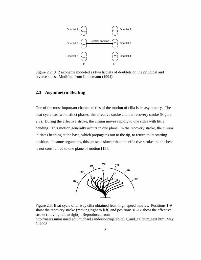
Figure 2.2: 9+2 axoneme modeled as two triplets of doublets on the principal and

reverse sides. Modified from Lindemann (1994)

2.3 Asymmetric Beating

One of the most important characteristics of the motion of cilia is its asymmetry. The

beat cycle has two distinct phases: the effective stroke and the recovery stroke (Figure

2.3). During the effective stroke, the cilium moves rapidly to one sides with little

bending. This motion generally occurs in one plane. In the recovery stroke, the cilium

initiates bending at the base, which propagates out to the tip, to return to its starting

position. In some organisms, this phase is slower than the effective stroke and the beat

is not constrained to one plane of motion [15].

Figure 2.3: Beat cycle of airway cilia obtained from high-speed movies. Positions 1-9

show the recovery stroke (moving right to left) and positions 10-12 show the effective

stroke (moving left to right). Reproduced from

http://users.umassmed.edu/michael.sanderson/mjslab/cilia_and_calcium_text.htm, May

7, 2008

Doublet 2

Doublet 3

Doublet 4 Doublet 7

Doublet 9

Doublet 8 Central partition

P R

9

2.4 Active vs. Passive Bend Mechanism

To determine whether cilia and flagella are active organelles, which can self-induce

motion, or passive organelles, which require the cell to initiate motion, three hypotheses

have been proposed: the passive microtubule mechanism, the active contractile

microtubule mechanism, and the active sliding microtubule mechanism. The passive

microtubule mechanism assumes that flagella are incapable of self-induced bend

initiation and propagation. Instead, it must rely on a signal within the cell to initiate

bending of the organelle at the base through the act of elastic microtubules.

Experimental evidence has shown that cilia and flagella do not require the cell body to

signal their motion, thus these organelles must be active elements [16]. The second

hypothesis, the active contractile microtubule mechanism, assumes the flagellum is

made of "active contractile microtubules" [15] that are able to change their length

relative to the other microtubules. Local contraction at a point along the flagellum then

causes bend initiation in that region. Thus, for this mechanism bend propagation occurs

as a result of the propagation of contraction of the active region. The active sliding

mechanism assumes the length of microtubules remains constant and they slide relative

to one another. This sliding produces inhomogeneous shear along the flagellum that

causes bending in adjacent regions [15].

In the active contractile mechanism, the microtubule on the outside of a bend will

change its position relative to the inner microtubule. The active sliding mechanism,

however, predicts that the microtubule on the inside of the bend will move tipward

relative to the outer microtubule. Electron-microscope observations strongly support

the active sliding mechanism [15].

Since bending is the result of sliding between adjacent doublets due to dynein arms

from the A-subtubule sliding against the B-subtubule of the higher numbered adjacent

doublet, there are only two possible directions of sliding (Figure 2.4). In the first case,

10

the dynein arms from doublet N generates force from base to tip on doublet N+1,

causing the higher numbered doublet to slide tipward. In the second case, active force

generation is from tip to base, causing the higher numbered doublet to slide baseward.

Experimental evidence supports the first case only. That is, one doublet's dynein arms

push its higher numbered adjacent doublet tipward [16].

Tip

Base

Doublet N+1 Doublet N

Dynein

armsA-subtubule

B-subtubule

Tip

Base

Doublet N+1Doublet N

Tip

Base

Doublet N+1 Doublet N

Case 1 Case 2

Figure 2.4: Illustration of possible bend directions: In case 1, sliding is tipward and in

case 2, sliding is baseward. Reproduced from Sale and Satir (1977)

2.5 Mechanics of Ciliary Bending

2.5.1 Basic Modeling Assumptions

To create the models used in this study, several assumptions and simplifications were

made. First, the cilium is modeled as a thin, flexible beam of constant length, L. The

distance along the flagellum is measured by the parameter s, where 0 ≤ s ≤ L. By

modeling the fluid motion as flow over a circular cylinder, it can be shown that the

11

Reynolds number for such flow is very small. As a result, it is sufficient to only

consider the viscous forces and neglect the inertial forces [15]. Thus, the only external

forces acting on the cilium are those from its viscous environment. Consistent with

previous studies, it is assumed that the dynein arms provide the active forces that allow

bending and passive elastic resistance comes from the radial spokes and/or nexin links.

2.5.2 Effects of Sliding

The mechanics derived in this study are based on the active sliding of neighboring

doublets. Bending is the result of dynein arms continuously pushing against

neighboring doublets, causing them to slide. Because the length of the cilium remains

constant, any sliding results in longitudinal shear between the doublets [5]. Each time

the microtubules slide and cause the cilium to bend, the new shape of the cilium can be

defined by its bend angle, α(s,t), which is the angle of the tangent to the cilium.

Another angle measurement, the shear angle, γ(s,t), represents the local deformation of

an elements due to sliding. If the base is fixed, the shear angle and the bend angle are

equal (Figure 2.5).

u

dss

uu

dss

d

d

dss

Figure 2.5: Relationship between bend angle, (s,t), and shear angle, (s,t)

When an outer doublet slides relative to the central pair of microtubules or relative to its

neighboring doublets, the radial spokes and nexin links must stretch (Figure 2.6). As a

result of this stretching, some resistive forces will be generated. When the passive

ss

s

u

ds

s

u

ds

d

dss

uu

dss

d

u

1

1

tan

tan

when γ(0,t) = α(0,t) then

),(),( tsts

12

elements are modeled as linear springs, it is simple to calculate their passive force

contribution to bending. The dynein arms are the active elements so when one doublet

slides relative to another, the dynein arms contribute active forces. The combination of

these components creates a shear force between microtubule pairs that causes an active

moment. This net effect can be treated additively so that the total internal force from

active and passive elements, fI, can be expressed as fI = factive+fpassive.

(a) (b)

Figure 2.6: Stretch of radial spokes: (a) Three-dimensional (3D) illustration of cilia

structure. Reproduced from

http://micro.magnet.fsu.edu/cells/ciliaandflagella/images/ciliaandflagellafigure1.jpg,

October 23, 2008

(b) Exploded view of stretch of radial spokes between central pair and outer doublets

due to sliding

To understand how the internal elements affect the motion of the cilium, the cilium can

be thought of as a simple cantilever beam (Figure 2.7). If a simple cantilever beam is

given an initial deflection by applying some force, the free end will vibrate at a constant

amplitude without the motion dying out. However, if this beam is put in some viscous

fluid and given the same initial displacement, the free end will initially vibrate but will

experience heavy damping, causing the motion to eventually die out. This scenario is

similar to considering the flagellum as only having passive elements, like the radial

spokes or nexin links. Next, if the cantilever beam is kept in the viscous fluid but now

has some active feedback mechanism, the free end will be able to vibrate throughout

R

R+ΔR ui-uo

Central

pair

Outer

doublet

13

time with increasing amplitude of oscillation. This is what happens when the effects of

the dynein arms are considered. The dynein arms provide active feedback to allow the

cilium to continue to oscillate while the radial spokes and nexin links provide resistance

to this bending. A central question to the study of motion of cilia and flagella is what

type of feedback, or regulation, from the dynein arms is needed to produce the observed

motion?

(a) (b) (c)

Figure 2.7: Conceptual depiction of active feedback required for sustained oscillations:

(a) a cantilever beam with no viscous forces; (b) a cantilever beam submerged in a

viscous fluid with no active feedback; and (c) a cantilever beam submerged in a viscous

fluid with an active feedback mechanism

When the internal elements cause the active shear, the beam will respond with an elastic

moment that resists bending, Me. For a beam in bending, this moment is proportional to

curvature and the flexural stiffness. That is, s

EM be

, where Eb is the flexural

stiffness. When looking at a segment of a pair of doublets, internal forces from one

segment to the other must also be considered. This includes tension inside each doublet

14

along its longitudinal axis and internal shear along the transverse axis. The viscous

forces incorporate the effect of the external environment on the motion of the cilium.

2.5.3 Free Body Diagrams and Derivation of Equations

The table below summarizes the variables used in the diagrams and equations in this

section.

15

Table 2.1: List of variables and their descriptions

Variable Description

( )N Component of ( ) in normal direction

( )T Component of ( ) in tangential direction

d Distance between doublets

2b Diameter of one doublet

R Distance between central pair and outer doublets

u Shear displacement due to sliding

α Angle between tangent to flagellum and the horizontal

γ Shear angle

Me Total internal elastic bending moment

M1 Internal elastic bending moment in doublet N

M2 Internal elastic bending moment on doublet N+1

FN Total internal transverse shear exerted from one segment onto neighboring

segment

FN1 Internal transverse shear exerted from one segment onto neighboring

segment on doublet N

FN2 Internal transverse shear exerted from one segment onto neighboring

segment on doublet N+1

FT Total longitudinal tension on segment

FT1 Longitudinal tension on doublet N

FT2 Longitudinal tension on doublet N+1

fIN Transverse force per unit length due to active and passive cell structures

between microtubule pairs

fIT Longitudinal force per unit length due to active and passive cell structures

between microtubule pairs

φN1 Normal external viscous force per unit length on doublet N

φN2 Normal external viscous force per unit length on doublet N+1

φT1 Tangential external viscous force per unit length on doublet N

φT2 Tangential external viscous force per unit length on doublet N+1

FE Total elastic force from stretch of nexin links

FET Longitudinal component of elastic force from stretching

FEN Transverse component of elastic force from stretch

The shape of the cilium at any point in time can be found by balancing the external

viscous moment, the internal bending moment, and the active moment generated from

the structural elements. To do this, it is necessary to examine the forces and moments

on a segment of the flagellum with free body diagrams (FBDs) (Figures 2.8 and 2.9).

η

16

ds

2

11

ds

s

FF T

T

2

22

ds

s

FF T

T

2

22

ds

s

FF T

T

2

11

ds

s

FF T

T

2

ds

s

MM e

e

2

ds

s

MM e

e

2

ds

s

FF N

N

2

ds

s

FF N

N

N̂

T̂

d

dsN 2

dsN1

dsT1

dsT 2

Figure 2.8: Total FBD of forces and moment acting on an element of the cilium

The forces and moments can be studied more thoroughly by examining each doublet

(Figure 2.9).

17

Doublet N

Doublet N+1

2

11

ds

s

FF T

T

2

11

ds

s

FF T

T

2

22

ds

s

FF T

T

2

22

ds

s

FF T

T

2

11

ds

s

MM

2

11

ds

s

MM

2

22

ds

s

MM

2

22

ds

s

MM

2

11

ds

s

FF N

N

2

11

ds

s

FF N

N

2

22

ds

s

FF N

N

2

22

ds

s

FF N

N

2

ds

s

2

ds

s

2

ds

s

2

ds

s

dsN1

dsN 2

dsT 2

dsT1

dsf IN

dsf IN

dsf IT

dsf IT

dsf IT

dsf IT

N̂

T̂

b2

b2

Figure 2.9: Exploded FBD of internal and external forces and moments on adjacent

doublets

Force balance in the normal and tangential directions and moment equilibrium yield the

following equations.

011

1

sF

s

Ff T

NINN

(2.1)

011

1

sF

s

Ff N

TITT

(2.2)

011

1

NITT F

s

Mbfb

(2.3)

022

2

sF

s

Ff T

NINN

(2.4)

18

022

2

sF

s

Ff N

TITT

(2.5)

022

2

NITT F

s

Mbfb

(2.6)

Combining Eqs. (2.1) with (2.4), (2.2) with (2.5), and (2.3) with (2.6), yields

sF

s

FT

NN

(2.7)

s

F

sF T

NT

(2.8)

bbfs

MF TTIT

eN 122

(2.9)

where φN and φT are the net normal and tangential external viscous forces such that

21 NNN and 21 TTT .

All of the theoretical models examined in this thesis make use of the force and moment

balances found in Eqs. (2.7)-(2.9). The way these models differ is in how they specify

the forces from the internal elements. Different ways of describing the force

contributions from the dynein arms, radial spokes, and nexin links will be discussed in

the next chapters.

19

2.6 Shear Growth Analysis

2.6.1 Mathematical Model

To illustrate the principle of shear deformation causing bending, a plane stress model of

a vertical beam with a specified growth law was developed. The modeling parameters

used in this model are described in the table below.

Table 2.2: Numerical modeling parameters for shear growth analysis

Solver type Time dependent

Element type Lagrange quadratic

Temporal discretization 0.02 sec

Relative tolerance 0.0001

Absolute tolerance 0.00001

The position of each particle of the 2D system at t0, called the reference configuration,

is described by ),( YXXX and the position of each particle after t0, called the spatial

description, is described by ),( YXxx [10]. The total deformation of the system can

be described by its the overall deformation gradient tensor, F~

. This deformation tensor

is related to the growth deformation gradient tensor, G~

, and the elastic deformation

gradient tensor, E~

. That is, GEF~~~ , where the total deformation gradient tensor is

defined in Cartesian coordinates by

smpssmps

smpssmps

FF

FF

Y

y

X

yY

x

X

x

F_22_21

_12_11~

(2.10)

20

The growth deformation gradient tensor describes the growth in the spatial description

with respect to the reference configuration. For example, if the beam was specified to

grow by an amount λ in the y-direction, then the growth deformation gradient tensor

would be

0

01~G . For this system, a shear growth, λg, is specified so the growth

tensor is

1

01~

g

G

(2.11)

The elastic deformation gradient tensor can be found from the overall deformation

gradient and the growth deformation tensors, so

1~~~ GFE (2.12)

where

1

01~ 1

g

G

.

The material is modeled as a neo-Hookean compressible material. The constitutive

equation for the strain energy for such a material is

21 12

32

Jk

IW

(2.13)

where μ and k are constants and 1I and J are related to the strain invariants of the elastic

right Cauchy-Green strain tensor EEC T ~~~ .

Next, the growth law can be specified. The total shear deformation, λg, at a point along

the beam is the cumulative sum of the local growth parameter, β, so

21

s

g

(2.14)

For a vertical beam, as discussed here, s is the same as the axial coordinate Y.

The local growth parameter varies with time as

)(1

tft

(2.15)

where f(t) is some forcing function. The local growth parameter represents local dynein

activity.

2.6.2 Simulation Results

The simulation described above was run for three different scenarios corresponding to

different functions for β. In the first case, the function f(t) in Eq. (2.15) is zero, except

at the base, so that the shear angle is constant (Figure 2.10). In the second case, the

forcing function is a constant, so that the equilibrium shear angle is a linear function of

the axial coordinate, Y, and curvature is constant (Figure 2.11). In the third case, the

forcing function is a sinusoidal function of time, that is constant in space, so that the

curvature oscillates (Figure 2.12).

22

Figure 2.10: Shear deformation when β=0 (except at the base) at t = 1 s and λg=constant

(except at the base).

Figure 2.11: Shear deformation when β is constant at t = 1 s and λg is a linear function

of Y (except at the base)

23

(a) (b) (c)

(d) (e) (f)

Figure 2.12: Shear deformation when β is a sinusoidal function of time: (a) t = 0 s, (b)

t = 0.2 s, (c) t = 0.4 s, (d) t = 0.6 s, (e) t = 0.8 s, and (f) t = 1.0 s

24

2.6.3 Simulation Discussion

The results from the shear deformation simulations confirm the assumption that shear

displacement between doublets will cause bending. It can be seen that when the local

shear deformation is zero, as in Figure 2.10, the cumulative shear deformation is

constant along the length of the beam. This causes the entire beam to bend at the same

angle with no significant curvature. When the local shear deformation is a constant, as

in Figure 2.11, the total shear deformation varies linearly with distance along the beam.

The curvature remains mostly constant throughout the length of the beam. In the third

case, the forcing function is a sinusoidal function, and thus so is the total shear

deformation. Unlike the previous two cases, this allows the beam to oscillate from one

side to the other, as shown in Figure 2.12. Since the local shear growth, β, represents

local dynein activity and the total shear deformation, λg, represents the total shear, it can

be seen that local activity controls curvature and total shear.

2.7 Conclusion

In this chapter, the basic structure of cilia and flagella is introduced in order to describe

the internal force generating elements. Equilibrium force and moment balances are

analyzed on doublets to derive the governing mechanics equations. A shear growth

model simulation is included to illustrate how shear displacement can cause bending in

a beam. The equations derived and the principles discussed in this chapter are used in

the following chapters' theoretical implementation of cilia and flagella motion. While

each of the following models uses the same principles as those discussed here, the main

differences lie in the representation of active and passive forces.

25

3 Curvature-Controlled Modeling

3.1 Introduction

The first model analyzed in this thesis is the curvature-controlled model by Hines and

Blum (1978). The goal of this theoretical model is to produce stable bend initiation and

propagation for a flagellum of fixed length. One of the key features is a realistic

representation for the shear resistance from the radial spokes based on large sliding

displacements and the geometry of the organelle. A stability analysis was conducted to

determine the necessary conditions on flexural stiffness and feedback gain required to

produce sustained oscillations [9]. This basic curvature-controlled model has been

unable to reproduce key features of ciliary and flagellar behavior, but it introduces a

number of concepts that are important in modeling these structures.

3.2 Mathematical Model

3.2.1 Derivation of Equations

This model is based on a set of nonlinear differential equations that are derived from

force and moment balances. The position of any point along the flagellum, s, at any

time, t, is represented by r(s, t) and the angle of the flagellum's tangent at any point and

time is represented by α(s, t). To model the viscous forces on the flagellum, the Gray-

Hancock approximation was used to relate the normal and tangential viscous forces to

the normal and tangential velocities along an element of length ds. That is,

26

dsVCdsts NNN ),( (3.1)

dsVCdsts TTT ),( (3.2)

where VN and VT are the normal and tangential velocities and CN and CT are the normal

and tangential viscous drag coefficients, respectively. It can be shown from Figures 2.8

and 2.9 and Eqs. (2.1)-(2.9) that

sF

s

FT

NN

(3.3)

s

F

sF T

NT

(3.4)

where FN and FT are the net external normal and tangential forces on the element. The

sign convention used by Hines and Blum (1978) is opposite the sign convention used in

the derivations of Chapter 2. Here, FN and FT represent the external forces on the

axoneme, while Eqs. (2.1)-(2.9) represent the internal forces.

By equating Eqs. (3.1) and (3.2) with Eqs. (3.3) and (3.4), expressions for the normal

and tangential velocity can be found.

sF

s

F

CV T

N

N

N

1

(3.5)

sF

s

F

CV N

T

T

T

1

(3.6)

The elastic moment in the flagellum, Me, in Eq. (2.9) can be related to its flexural

stiffness, Eb, by

27

sE

s

Mb

e

(3.7)

where κ is the curvature of the element. If the viscous forces of Figures 2.8 and 2.9 are

distributed evenly on either side of the axoneme so that TTT 2

121 and

NNN 2

121 , then substituting Eq. (3.7) into Eq. (2.9) yields

Ss

EF bN

2

2

(3.8a)

where bfS IT2 represents the effective "shear force" from the internal cellular

elements. Hines and Blum (1978) then, for consistency with earlier work, define FN to

be the negative of the expression in Eq. (3.8a) (i.e., as the net external force on the

flagellum distal to the element), so

Ss

EF bN

2

2

(3.8b)

By taking the spatial derivative of the velocity at any point on the flagellum, Hines and

Blum (1978) obtain

sV

ts

VT

N

(3.9)

sV

s

VN

T

(3.10)

Differentiating Eqs. (3.5) and (3.6) with respect to the spatial variable, s, and equating

those expressions with Eqs. (3.9) and (3.10) yields

28

2

22

2

2

1s

Fs

FC

C

ss

F

C

C

tC

s

FTN

T

NT

T

NN

N

(3.11)

2

22

2

2

1s

Fs

FC

C

ss

F

C

C

s

FNT

N

TN

N

TT

(3.12)

In Eqs. (3.8a) and (3.8b), the effective shear is the sum of the active shear from the

dynein arms and the passive shear from the radial spokes, so S = Sd + Sr. In this model,

the shear force from the radial spokes is a function of the shear angle, γ(s,t).

2

1

1

1

11

BASr

(3.13)

where A1 and B1 are constants that depend on the geometry of the flagellum. The

contribution of the dynein arms is modeled as a two-parameter partial differential

equation which represents a hypothetical dependence of dynein activity on local

curvature.

dd S

sm

t

S

0

(3.14)

where τ is a time constant and m0 is a feedback gain that describes the dependence of

dynein activity on curvature.

3.2.2 Simulation Procedures

To model the motion of the flagellum, Eqs. (3.8b), (3.11), (3.12) and (3.14) were

entered as partial differential equations in COMSOL Multiphysics to determine the

29

forces and shape of the flagellum at various times. The table below describes the

modeling parameters used for the finite element model simulation.

Table 3.1: Numerical modeling parameters for curvature-controlled model

Solver type Time dependent

Element type Lagrange quadratic

Number of spatial elements 100

Temporal discretization 0.001 sec

Relative tolerance 0.001

Absolute tolerance 0.0001

The results were post-processed in MATLAB to interpret the resulting motion. Table

3.1 shows the values used for each parameter in this model, unless otherwise noted.

Table 3.2: Constant values for curvature-controlled model

Parameter Value Used

A1 65 pN

B1 0.75

CN 0.005 pN s/µm2

CT 0.0025 pN s/µm2

τ 0.02 s

Eb 30 pN μm2

m0 130 pN μm

3.2.3 Stability Analysis Procedures

Once a computer model was created that produced sustained wave propagation, a

stability analysis was conducted to determine the effects of the feedback gain, m0, and

30

flexural stiffness, Eb, on the motion of the flagellum. To do this, the nonlinear terms are

eliminated from Eqs. (3.11) and (3.8b) is substituted for FN to yield

2

2

4

41

s

S

sE

Ct

db

N

(3.15)

Using Eqs. (3.14) and (3.15) and assuming an exponential form for the solution of α and

Sd, the equations can be put in matrix form.

tiks

dd

eeSS

0

0

(3.16a)

0

0

0

24

0

0

1

1

d

NN

b

d Skim

kCC

kE

S

(3.16b)

where k is the wave number. Eq. (3.16b) is an eigenvalue problem and can be solved

for λ. From this, the critical values of Eb and m0 can be found.

3.2.4 Simulation Results

The first result is to see the effects that radial spokes and dynein arms have on the

motion of the flagellum. Figure 3.1 shows the resulting motion for the flagellum

without and with the contribution of the radial spokes.

31

0 10 20 30-15

-10

-5

0

5

10

15

X (m)

Y (

m)

0 10 20 30-15

-10

-5

0

5

10

15

X (m)

Y (

m)

(a) (b)

Figure 3.1: Wave propagation of flagellum for t=0.24 to t=0.25 sec (a) without the

contribution of radial spokes and (b) with the contribution of the radial spokes

The graphs in Figure 3.2 show how wave propagation changes as a result of varying the

viscous drag coefficients.

32

(a)

0 5 10 15 20 25 30-4

-2

0

2

4

X (m)

Y (

m)

0 5 10 15 20 25 30-4

-2

0

2

4

X (m)

Y (

m)

0 5 10 15 20 25 30-4

-2

0

2

4

X (m)

Y (

m)

0 5 10 15 20 25 30-4

-2

0

2

4

X (m)

Y (

m)

AP=5.02 μm

(b) AP=4.53 μm

(c) AP=4.67 μm

(d) AP=4.55 μm

Figure 3.2: Wave propagation plots for t=0.24 to 0.25 seconds for various values of

drag coefficients CN and CT (peak-to-peak amplitude: AP). (a) CN=0.005 pN s/μm2,

CT=0.0025 pN s/μm2; (b) CN=0.0025 pN s/μm

2, CT=0.005 pN s/μm

2; (c) CN=CT=0.005

pN s/μm2; (d) CN=0.05 pN s/μm

2, CT=0.025 pN s/μm

2

33

3.2.5 Stability Analysis Results

In many problems, unstable behavior is undesirable because the system does not die out

and is harder to keep under control. For a beating flagellum, however, local (linearly)

unstable behavior is necessary for sustained oscillations with increasing peak-to-peak

amplitudes. In this situation, the nonlinear stiffness of the radial spokes restrains the

amplitude of motion.

The stability analysis results showed that for sustained oscillations, k

km13

0 ,

where Nb

N

b CEC

E and

NbCE

1 . From these expressions, the maximum

flexural stiffness, Eb, can be found as well (Figure 3.3)

-2 0 20

200

400

600

800

k (m-1)

Eb (

pN

m

2)

-1 0 1-100

-50

0

50

100

k (m-1)

m0 (

pN

m

)

(a) (b)

Figure 3.3: Stability analysis plots showing (a) the maximum flexural stiffness, Eb, for

sustained oscillations vs. the wave number, k, and (b) the minimum feedback gain for

dynein activity, m0, for sustained oscillations vs. the wave number, k.

34

Simulations were performed to evaluate the predictions of the stability analysis. To

observe the effect of flexural stiffness on the motion of the flagellum, the wave

propagation for various values of Eb were examined (Figures 3.4 and 3.5). A similar

simulation protocol was followed to observe the effects of varying the feedback

constant, m0 (Figures 3.6 and 3.7).

35

(a)

0 5 10 15 20 25 30-4

-2

0

2

4

X (m)

Y (

m)

0 5 10 15 20 25 30-4

-2

0

2

4

X (m)

Y (

m)

0 5 10 15 20 25 30-4

-2

0

2

4

X (m)

Y (

m)

0 5 10 15 20 25 30-4

-2

0

2

4

X (m)

Y (

m)

AP=4.52 μm

(b) AP=5.02 μm

(c) AP=4.19 μm

(d) AP=1.25 μm

Figure 3.4: Wave propagation plots for t=0.24 to 0.25 seconds for various values of Eb

(peak-to-peak amplitude: AP). (a) Eb=10 pN μm2; (b) Eb=30 pN μm

2; (c) Eb=50 pN μm

2;

and (d) Eb=100 pN μm2

36

(a)

0 0.05 0.1 0.15 0.2 0.25-1

0

1

Time (sec)

(

rad)

0 0.05 0.1 0.15 0.2 0.25-1

0

1

Time (sec)

(

rad)

0 0.05 0.1 0.15 0.2 0.25-1

0

1

Time (sec)

(

rad)

0 0.05 0.1 0.15 0.2 0.25-1

0

1

Time (sec)

(

rad)

(b)

(c)

(d)

Figure 3.5: Cross-section plots of bend angle vs. time at s=15 μm for various values of

Eb: (a) Eb=10 pN μm2 (b) Eb=30 pN μm

2 (c) Eb=50 pN μm

2 and (d) Eb=100 pN μm

2

37

(a)

0 5 10 15 20 25 30-4

-2

0

2

4

X (m)

Y (

m)

0 5 10 15 20 25 30-4

-2

0

2

4

X (m)

Y (

m)

0 5 10 15 20 25 30-4

-2

0

2

4

X (m)

Y (

m)

0 5 10 15 20 25 30-4

-2

0

2

4

X (m)

Y (

m)

AP=1.07 μm

(b) AP=3.10 μm

(c) AP=5.02 μm

(d) AP=6.51 μm

Figure 3.6: Wave propagation plots for t=0.24 to 0.25 seconds for various values of m0

(peak-to-peak amplitude: AP). (a) m0=35 pN μm; (b) m0=75 pN μm; (c) m0=130 pN μm;

(d) m0=200 pN μm

38

(a)

0 0.05 0.1 0.15 0.2 0.25-1

-0.5

0

0.5

1

Time (sec)

(

rad)

0 0.05 0.1 0.15 0.2 0.25-1

-0.5

0

0.5

1

Time (sec)

(

rad)

0 0.05 0.1 0.15 0.2 0.25-1

-0.5

0

0.5

1

Time (sec)

(

rad)

0 0.05 0.1 0.15 0.2 0.25-1

-0.5

0

0.5

1

Time (sec)

(

rad)

(b)

(c)

(d)

Figure 3.7: Cross-section plots of bend angle vs. time at s=15 μm for various values of

m0: (a) m0=35 pN μm (b) m0=75 pN μm (c) m0=130 pN μm (d) m0=200 pN μm

3.2.6 Discussion

From Figure 3.1, it can be seen that the radial spokes do in fact provide passive elastic

resistance to bending while the dynein arms provide the active forces needed for bend

initiation. When the flagellum lacks radial spokes, but still has dynein arms, the motion

is random and the organelle gets twisted in itself. With the contribution of both the

dynein arms and radial spokes, stable, organized propagations occur.

The ratio of the viscous drag coefficients is included in Eqs. (3.11) and (3.12), and thus

affects the motion. This model produces continuous oscillations for various values of

drag coefficients. Figure 3.2a shows the most realistic case, where CN is twice the value

39

of CT, though a ratio of 1.8 may be more accurate [9]. In Figure 3.2b, CN is less than

CT. resulting in decreased peak-to-peak amplitude. The wave propagation for this

scenario is out of phase with that resulting from a ratio of 2. When the values of CN and

CT are equal, the peak-to-peak amplitude decreases without significant frequency

changes. When both drag coefficients are ten times as large as their original value, as in

Figure 3.2d, the frequency increases significantly. Hines and Blum (1978) suggest that

when the ratio is held at 2 but the value of CN increases, the frequency decreases until

CN exceeds 0.03, then it will increase [9]. This is consistent with the results found in

this study.

From the stability analysis on Eb, it can be seen that when the flexural stiffness is

decreased, wave propagation continues but at a higher frequency and slightly smaller

amplitude. However, when Eb is increased, it is more difficult to produce continuous

oscillations. The period of oscillation increases, causing the frequency and the peak-to-

peak amplitude to decrease (Figure 3.4). These effects can also be seen by examining

plots of bend angle versus time at a fixed point along the flagellum (Figure 3.5). When

Eb is low enough to allow sustained oscillations, the bend angle starts small and

increases until it reaches steady-state. As the flexural stiffness decreases, the frequency

of oscillation for the bend angle increases.

The results from the stability analysis on m0 show that if this constant is too low, the

flagellum has difficulty producing sustained oscillations. The force from the dynein

arms is directly related to this constant. If the dynein arms are unable to reach a certain

threshold, it will be difficult to produce the wavelike motion that is characteristic of a

beating flagellum. Decreasing m0 decreases the amplitude and increases the period of

oscillation. When m0 is increased above the critical value, the flagellum is able to

produce wave propagation with increasing amplitude until it reaches steady state.

Increasing m0 has similar effects on the frequency and peak-to-peak amplitude as

decreasing Eb .

40

From the equations that result from the force and moment balances in this model, it is

important to realize that once the difference in sign convention is accounted for, Eqs.

(3.3) and (3.4) are analogous to Eqs. (2.7) and (2.8) derived in Chapter 2. Further, if the

viscous forces are distributed evenly on either side of the axoneme such that 21 TT ,

then Eqs. (2.9) and (3.8) are also analogous.

One major advantage of this model is that a stability analysis can be performed to

predict conditions under which sustained oscillations will occur. The predictions of the

stability analysis are confirmed by the simulation, which builds confidence in the

accuracy of both the analysis and the COMSOL model. Once a more accurate

mathematical model is created, the effects of changing the flexural stiffness on the

motion of the cilium can be compared to laboratory results from using drugs like Taxol

that stiffen the doublets. This would provide a useful comparison for the theoretical and

experimental results.

While this model does produce continuous oscillations for various values of modeling

parameters and the mechanics are accurately represented by the differential equations,

some shortcomings remain. The shear from the radial spokes in this model is based on

the geometry of the flagellum but the active shear contribution from the dynein arms is

not based on any known biophysical mechanism. For this model, Hines and Blum

(1978) chose a simple curvature feedback law to represent the active shear from the

dynein arms. A more appropriate model would incorporate some biophysical

explanation for how and when the dynein arms attach. This model also lumps the

affects of the nexin links into the expression for shear force from radial spokes. A

possible improvement would be to explicitly incorporate their contribution to the

passive shear. Another flaw in this model, in its current state, is that it does not

accurately represent the asymmetry of the flagellar beat.

41

3.3 Conclusion

The purpose of this model in the current study was to use a set of nonlinear differential

equations to see if the wavelike motion could be produced in a basic model of a

flagellum. This model is a useful introduction to understanding the mechanics that

drive cilia and flagella motion. The main benefits of this model are that it is simple

enough to conduct a stability analysis on and the mechanics are reliable. The main

problem is that it does not accurately represent the biophysical mechanisms that govern

the internal elements, especially the control function of the dynein arms, which may

help produce an asymmetric beat. The model described in the next chapter improves on

the dynein force contribution but fails in having reliable mechanics. A combination of

the mechanics described in this chapter with a more accurate active shear force

contribution would produce a superior model.

42

4 Interdoublet Spacing Controlled Mechanism

4.1 Introduction

It is well known that dynein arms provide the motility needed for bend propagation in

cilia and flagella but what controls their activity is not as well understood. In this

chapter, a model that assumes dynein engagement is controlled by interdoublet spacing

is examined. The model discussed here uses a geometric mechanism to describe and

control dynein arm activity and is essentially identical to one proposed by Lindemann

(1994).

4.2 The "Geometric Clutch" Hypothesis

4.2.1 Objectives

The geometric clutch hypothesis proposed by Lindemann (1994) assumes that dynein-

tubulin interaction is dependent primarily on the spacing between adjacent doublets.

The interdoublet spacing is controlled by internal forces that act transverse to the

longitudinal axis of the flagellum, which Lindemann (1994) calls "t-forces". When the

internal transverse forces are large enough, the doublets are pulled close enough

together that dynein arms can attach, forming force producing cross-bridges. Activated

dynein arms cause sliding between the outer doublets, which leads to bending.

Alternatively, when the interdoublet spacing becomes too large, dynein arms will

detach, terminating the sliding episode [12, 13]. The goal of this model is to produce a

43

computer simulation of ciliary and flagellar motion using these principles of transverse

forces and interdoublet spacing.

4.2.2 Methods

Modeling Assumptions

The computer model is developed from a code written by Lindemann (1994) to

implement the geometric clutch mechanism. To create the computer simulation for this

switching mechanism, several simplifications are employed. First, because of the stable

central partition and bridge between doublets 5 and 6, sliding occurs in the plane

perpendicular to the central pair only. Experimental evidence has proven that each

doublet's dynein arms push its higher-numbered neighbor tipward [12, 16]. As a result,

dynein arms on opposite sides of the axoneme will bend the axoneme in opposite

directions. For example, the arms on doublet 3 will push the 4, 5-6, 7 group of doublets

tipward while the arms of doublet 7 will push this same group of doublets baseward.

Experimental evidence has also shown that 60% of sliding occurs at the doublets closest

to the stable central partition, so the axoneme can be modeled as two triplets connected

by the partition, one on each side of the axoneme (2-3-4 on reverse side and 7-8-9 on

principal side).

44

A B

IPSIPS

(a)

BA

IRSIRS

(b)

Doublet 2

Doublet 3

Doublet 4Doublet

7

Doublet

9

Doublet

8

Central

partition

P R

A

AB

B

(c)

A B

IPSIPS

A B

IPSIPS

(a)

BA

IRSIRS

BA

IRSIRS

(b)

Doublet 2

Doublet 3

Doublet 4Doublet

7

Doublet

9

Doublet

8

Central

partition

P R

A

AB

B

(c)

Figure 4.1: Illustration of simplification of 9+2 axoneme as two triplets

To simplify the simulation of flagellar motion, four basic modeling assumptions are

made regarding the dynein arms. First, the dynein arms are in their activated state.

Second, dynein activation is assumed to be dependent on interdoublet spacing only.

Third, the force produced from engaged dynein arms are assumed to have longitudinal

and transverse force components. The longitudinal component drives sliding and the

transverse component provides adhesive forces that decrease spacing. Lastly, the force

contribution per activated dynein arm is assumed to be a constant. When large

numbers, N, of arms are engaged, their force contribution is assumed to be proportional

to N [13].

Mathematical Modeling

Passive bending on one side of the axoneme occurs all the time, but is dominant in the

time period between termination of and restoration of active sliding on that side.

Passive motion can also result from external forces and moments, such as viscous forces

[12]. During passive bending, the elastic nexin links stretch, resulting in resistive forces

in both the longitudinal and transverse directions (Figure 4.2). These forces are

45

sinEET FF (4.1)

cosEEN FF (4.2)

where FE is the total elastic force, α is the bend angle, FET is the longitudinal component

and FEN is the transverse component of the force, (Lindemann (1994) refers to FEN as

the "local t-force"). The transverse component of the passive force will decrease the

distance between the doublets. The change in spacing is proportional to the local t-

force, so

dKFE (4.3)

where K is a constant.

Figure 4.2: (a) Forces produced from stretch of elastic nexin links between adjacent

doublets (Reproduced from Lindemann (1994)) (b) Force produced from stretching

nexin links modeled as linear springs.

The longitudinal force component from stretching the nexin links contributes to a total

longitudinal force, FTotal. Treating the distal sum of the forces from the passive and

active elements additively yields

d

d+Δd

Δd FE

Resting nexin link

Stretched nexin link

1cos

1

))((

Kd

dddKFE

(b)

22 du

u = Shear displacement from sliding

d = Resting length of nexin link

h = Stretched length of nexin links = d/(cos α) =

Δd = Stretch of nexin links = h-d

α = Angle formed by nexin link

FE = Total elastic force from stretch of nexin link

FET = Longitudinal force component from stretch = FE sin α

FEN = Local transverse force component from stretch = FE cos α

(a)

Doublet N+1

Doublet N

h

u

d EF

ETF

ENF

d

46

AETTotal FFF (4.4)

where FA is the longitudinal force component from the active dynein arms. This total

longitudinal force can be used to find the contribution of the active and passive

elements to the transverse force. The free body diagram below is modified from

Chapter 2 to represent the forces that Lindemann (1994) assumes act on the principal

side of a segment of the axoneme. It is important to realize that this model neglects

some of the forces present in the free body diagram, such as the viscous forces and the

internal transverse shear, FN. The diagram of Figure 4.3 represents the forces and

moments on the left-hand side of Figure 4.4.

Doublet 9

Doublet 7

2

ds

s

FF Total

Total

2

ds

s

FF Total

Total

2

ds

s

FF Total

Total

2

ds

s

FF Total

Total

2

11

ds

s

MM

2

11

ds

s

MM

2

22

ds

s

MM

2

22

ds

s

MM

2

11

ds

s

FF N

N

2

11

ds

s

FF N

N

2

22

ds

s

FF N

N

2

22

ds

s

FF N

N

2

ds

s

2

ds

s

2

ds

s

2

ds

s

dsN1

dsN 2

dsT 2

dsT1

ENF

ETF

N̂

T̂

b2

b2

ETF

ETF

ETF

ENF

Figure 4.3: FBD showing forces acting on the triplet of doublets 7-9 on the principal

side

47

PRETTRETRRTotal

RPETTRETPPTotal

RPETTop

RPTR

FFFFFFF

FFFFFFF

FFFF

FFF

)1(

)1(

2

)(

,

,

Figure 4.4: Longitudinal forces acting at each segment of the flagellum

Lindemann (1994) calls the transverse force generated from the combination of the

longitudinal force components of the active and passive elements the "global t-force".

From the free body diagram, it is clear that the transverse component of FTotal on each

doublet is

Global t-force = TotalFs

(4.5)

Further, it can be seen that for this model, the total transverse force on either side is the

sum of this global t-force and FEN.

Dynein arms on opposite sides contribute longitudinal forces of opposite signs; so while

one side experiences increasing transverse forces, the other sides experiences

decreasing transverse forces. This causes continued dynein attachment on one side and

limited dynein attachment on the other [13]. The longitudinal force from the dynein

arms on the principal and reverse sides are FP and FR, respectively.

ETF

ETF

PF

PFETF

ETFRF

RF

TRF

TRF

Positive force out of page

Negative force into page

48

According to Lindemann (1994), during bending there is some transfer of active force

from one side to the other via nexin links. When the principal side is actively bending,

the reverse side may be passively bending but will also have some force contribution

from the engaged arms on the principal side. This force transfer must be considered

when calculating the total longitudinal force on either side of the flagellum (Figure 4.4).

Active sliding on one side tends to unbend the existing curvature, causing the

interdoublet spacing on that side to increase, which will end that episode of sliding.

This allows the passive bend on the opposite side to transition into an active bend as

interdoublet spacing decreases and dynein arms attach.

Attached bridges also contribute an adhesive force that resists detachment and further

doublet separation. As engaged bridges detach, this force contribution becomes smaller

and causes the detachment to spread along the length of the axoneme. This results in

one side having no interdoublet tension so the active bend will become a passive bend

and dynein arms on the opposite side will begin to attach.

Computer Simulation

To create a computer simulation of this theory, the algorithm derived by Lindemann

(1994) is closely followed. In the algorithm, the flagellum is modeled as 30 segments

of equal length. Initial angles are provided for each segment which determine the initial

positions, curvature, and shear angles. The angles, positions, and curvature are

readjusted throughout each iteration based on the internal force distribution. The

passive force components can be found from the shape of the flagellum. This is then

used to find the total longitudinal and transverse forces from active and passive

elements. At each segment, n, the total longitudinal force on the top or bottom of the

flagellum can be calculated from Figure 4.4 by

49

30 30 30

2)(n n n

RPET FFFnF (4.6)

This longitudinal force is multiplied by the effective diameter to calculate the total

torque acting on the segment, which is then used to find the equilibrium curvature:

DnFEIds

d )(0

(4.7)

where I0E is the stiffness and D, the effective diameter, is the spacing between doublets

2-4 and doublets 7-9.

The total internal transverse force acting on the principal and reverse sides of each

segment is the distal sum of the active and passive components of the transverse force.

From Figures 4.3 and 4.4 and Eq. (4.5), the total transverse force on either side of the

axoneme can be found by,

Total t-forceP(n)=

RP

ni

ETEN FFiFds

dnF

)1()()(

30

(4.8)

Total t-forceR(n)=

PR

ni

ETEN FFiFds

dnF

)1()()(

30

(4.9)

where is the constant force transfer factor.

In the computer simulation, a random number is generated for each dynein head on each

segment. This number is compared to the probability of dynein arm attachment to

determine which arms will attach. The base probability is modified by the total

transverse force at each segment to determine the active probability of attachment. On

the principal and reverse sides, the active probability is found by

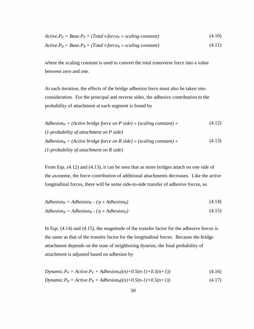
50

Active.PP = Base.PP + (Total t-forceP scaling constant) (4.10)

Active.PR = Base.PR + (Total t-forceR scaling constant) (4.11)

where the scaling constant is used to convert the total transverse force into a value

between zero and one.

At each iteration, the effects of the bridge adhesion force must also be taken into

consideration. For the principal and reverse sides, the adhesive contribution to the

probability of attachment at each segment is found by

AdhesionP = (Active bridge force on P side) (scaling constant)

(1-probability of attachment on P side)

(4.12)

AdhesionR = (Active bridge force on R side) (scaling constant)

(1-probability of attachment on R side)

(4.13)

From Eqs. (4.12) and (4.13), it can be seen that as more bridges attach on one side of

the axoneme, the force contribution of additional attachments decreases. Like the active

longitudinal forces, there will be some side-to-side transfer of adhesive forces, so

AdhesionP = AdhesionP - ( AdhesionR) (4.14)

AdhesionR = AdhesionR - ( AdhesionP) (4.15)

In Eqs. (4.14) and (4.15), the magnitude of the transfer factor for the adhesive forces is

the same as that of the transfer factor for the longitudinal forces. Because the bridge

attachment depends on the state of neighboring dyneins, the final probability of

attachment is adjusted based on adhesion by

Dynamic.PP = Active.PP + AdhesionP((n)+0.5(n-1)+0.5(n+1)) (4.16)

Dynamic.PR = Active.PR + AdhesionR((n)+0.5(n-1)+0.5(n+1)) (4.17)

51

The final step is to simulate the effects of viscous drag on the flagellum. To do this, the

moment due to viscous drag at each segment is found from the sum of the drag on the

distal segments. That is,

Mdrag(n) =

i n

30

(drag coefficient V(i) Ln(i) s) (4.18)

where Ln is the lever arm and s is the segment length. The velocity at each segment,

V(i), is found by comparing the position of the segment’s endpoints at the previous and

current iterations. At each iteration, the drag coefficient is recalculated to ensure that

the flagellum is in equilibrium, which requires

Mactive + Melastic - Mdrag = 0 (4.19)

Based on the viscous drag, the positions are recalculated and stored. The simulation

then goes through this process for each iteration. The flow chart below summarizes the

different steps involved in the original simulation of the geometric clutch hypothesis by

Lindemann (1994).

Figure 4.5: Flowchart describing algorithm used for switching mechanism based on

interdoublet spacing and transverse forces

To compare the results of using this method of finding the viscous moment to a simpler

method, the model was modified to use the Gray-Hancock approximation. At each

52

iteration the x- and y-direction velocities are found by dividing the displacement in each

direction by the time step between iterations. The normal and tangential velocities and

viscous forces are then found from

VN Vx cos Vy sin (4.20)

VT Vx sin Vy cos (4.21)

sVC NNN (4.22)

sVC TTT (4.23)

where CN and CT are the normal and tangential viscous drag coefficients. To determine

the drag coefficients, the following equations are used

CT 4

1 log104cb

a2

(4.24)

2

410log1

8

a

cbCN

2CT

(4.25)

where a is the center-to-center distance between the outer doublets and the central pair,

is the viscosity of water, and the length of the flagellum varies from –c to b [11, 15].

Although the Gray-Hancock approximation is not the ideal way to represent viscous

forces, Lighthill (1976) asserts that by calculating optimal drag coefficient with Eqs.

(4.24) and (4.25), this suboptimal method may be used in some scenarios.

4.2.3 Results

The geometric clutch hypothesis was analyzed for four scenarios. The first uses the

original method for finding the viscous drag moment and recalculates the drag

53

coefficient at each iteration. The second uses the original viscous drag moment but

maintains a constant drag coefficient. The last two scenarios use the Gray-Hancock

approximation to find the viscous forces and moment but the third recalculates the drag

coefficients at each iteration and the fourth keeps CN and CT constant for each iteration.

The simulation for each of the four cases were run ten times each for 3000 iterations,

corresponding to a total time of 0.3 sec.

54

Table 4.1: Modeling parameters for simulated motion of cilium (Modified from

Lindemann (1994))

Total length (cm) 0.001

Number of segments 30

Segment length (cm) 3.33x10-5

Functional diameter between doublets 2-4 and 7-9 (cm) 1.0x10-5

Time for each iteration (sec) 0.0001

Original initial drag coefficient (dyne cm-2

sec) 0.028

Modified initial tangential drag coefficient, CT (g-cm-1

sec-1

) 0.0283

Modified initial normal drag coefficient, CN (g-cm-1

sec-1

) 0.0566

Passive stiffness of cilium, IE (dyne-cm2)

1.0x10-13

Elastic constant for nexin links (dyne/cm) 0.2

Force per active dynein head (dyne) 1.2x10-7

Dynein heads per modeling segment 130

Transaxonemal force transfer coefficient 0.14

Base probability of attachment on principal bend side 0.06

Base probability of attachment on reverse bend side 0.01

Transverse force scaling factor 7,000

Adhesive force scaling factor (principal and reverse sides) 33,000

55

-4 -2 0 2 4 6 8 10 12

x 10-4

-8

-6

-4

-2

0

2

4

x 10-4

X (cm)

Y (

cm

)

Figure 4.6: Shape history of cilium shown at every 75 iterations for original drag

algorithm with non-constant drag coefficient (Iterations 10 to 3000, approximately 25

cycles)

Table 4.2: Statistics for original drag algorithm with non-constant drag coefficient

Average x standard deviation 1.82x10-4

Average y standard deviation 1.71x10-4

Average minimum y amplitude (cm) 8.134x10-4

Average maximum y amplitude (cm) 5.95x10-4

56

Figure 4.7: Shape history of cilium shown at every 75 iterations for original drag

algorithm with constant drag coefficient (Iterations 10 to 3000, approximately 25

cycles)

Table 4.3: Statistics for original drag algorithm with constant drag coefficient

Average x standard deviation 1.87x10-4

Average y standard deviation 1.67x10-4

Average minimum y amplitude (cm) 8.53x10-4

Average maximum y amplitude (cm) 4.71x10-4

-4 -2 0 2 4 6 8 10 12

x 10-4

-8

-6

-4

-2

0

2

4

x 10-4

X (cm)

Y (

cm

)

57

Figure 4.8: Shape history of cilium shown at every 75 iterations for Gray-Hancock drag

algorithm with non-constant drag coefficients (Iterations 10 to 3000, approximately 25

cycles)

Table 4.4: Statistics for modified drag algorithm with non-constant drag

coefficients

Average x standard deviation 1.82x10-4

Average y standard deviation 1.77x10-4

Average minimum y amplitude (cm) 8.57x10-4

Average maximum y amplitude (cm) 3.13x10-4

-4 -2 0 2 4 6 8 10 12

x 10-4

-8

-6

-4

-2

0

2

4

x 10-4

X (cm)

Y (

cm

)

58

Figure 4.9: Shape history of cilium shown at every 75 iterations for Gray-Hancock drag

algorithm with constant drag coefficients (Iterations 10 to 3000, approximately 25

cycles)

Table 4.5: Statistics for modified drag algorithm with constant drag coefficients

Average x standard deviation 1.84x10-4

Average y standard deviation 1.76x10-4

Average minimum y amplitude (cm) 8.57x10-4

Average maximum y amplitude (cm) 3.27x10-4

4.2.4 Discussion

It can be seen that all four cases produce cilia-like motion with the characteristic

effective and recovery strokes. However, the original drag algorithm (Figure 4.6) with

-4 -2 0 2 4 6 8 10 12

x 10-4

-8

-6

-4

-2

0

2

4

x 10-4

X (cm)

Y (

cm

)

59

a non-constant coefficient does not seem to distinguish between these two phases as

well as the other three. The two cases that use the Gray-Hancock approximation

illustrate the distinction between these two phases best (Figures 4.8 and 4.9).

The standard deviation in the y-direction resulting from using the Gray-Hancock

approximation is slightly higher than that for the original drag algorithm. The largest

amplitudes in the y-direction occur for the original drag algorithm with a non-constant

drag coefficient. The maximum amplitudes in the y-direction are significantly

decreased when the Gray-Hancock approximation is used. When the Gray-Hancock

approximation is used or the original drag algorithm is used with a constant drag

coefficient, the cilium seems to push itself more towards the left (or the negative x-

direction). These changes may be due to moment imbalance causing the viscous forces

to push the flagellum in a certain direction.

One of the key features of this model is the inclusion of the adhesive contribution of the

dynein arms. Additionally, it incorporates how the activation state of nearby dynein

arms adjusts the probability for further dynein attachment. These two features are

unique ways to help characterize the switching mechanism for bend direction. It is

reasonable to assume that once the cilium is bent in one direction, the dynein arms near

the base will begin to detach, allowing for reversal of bend direction.

Despite its success in producing realistic motion, the geometric clutch model is suspect.

First, it is strictly a discrete model; to obtain more accurate results, more than 30

segments can be used. More importantly, the mechanics used in this model are

inconsistent and errors must be corrected before further analysis is used. For example,

the current simulation uses trial and error values of the drag at the base to enforce the

zero drag condition at the base. Also, the drag coefficient is recalculated during each

iteration in order to implement moment equilibrium. The drag coefficient is a parameter

that is related to a body’s surface area and viscous conditions and it is not accurate to

60

assume that such a value would vary in a real physical system. However, in this model,

when the drag coefficient maintains a constant value, there is no guarantee that the

system is in equilibrium.

If the free body diagram of Figure 4.3 and Eqs. (4.8) and (4.9) are compared to Figures

2.8 and 2.9, it can be seen that this model neglects the viscous forces and the internal

transverse force that each segment enforces on its neighboring segment.

When describing the side-to-side force transfer through the nexin links, there is some

inconsistency between the longitudinal forces and the adhesive forces. In Eq. (4.8), the

longitudinal force component on the principal side, FP, is multiplied by (1-) and the

longitudinal force component on the reverse side is multiplied by the transfer factor, .

However, in Eq. (4.14), the adhesive force contribution is multiplied by 1 and not by (1-

). The same is true for Eqs. (4.9) and (4.15). It does not seem correct that the

principal side adhesion contributes 100% of itself to the adhesion on the principal side

but also a certain fraction to the reverse side, and vice versa. Thus, Eqs. (4.14) and

(4.15) should be consistent with Eqs. (4.8) and (4.9). This model also has a few sign

errors. In the original algorithm, the FR term in Eqs. (4.8) and (4.9) is multiplied by

and 1 , which is inconsistent with the equations derived from the force diagram

of Figure 4.4.

The geometric clutch simulation models the passive nexin links as linear springs.

However, there is no incorporation of the effects of the radial spokes on the motion of

the flagellum. This model does not look at all nine outer doublets and instead focuses

on the two triplets connected to the central pair by the stable central partition. It can be

argued that because of this simplification, the radial spokes do not need to be included.

However, there must be some force contribution from these elements or the central

partition that can be represented by defining a more accurate passive force equation.

61

4.3 Conclusion

The geometric clutch model described in this chapter has several unique characteristics

that previous models do not include, including the effects of adhesion and a structural

simplification to two triplets on opposite sides of the axoneme. The main flaws of this

model are mechanical errors such as using trial and error techniques to enforce

boundary and equilibrium conditions and inconsistencies in equations throughout the

algorithm. Lindemann (1994) uses non-standard algorithms to simulate the motion of

the cilium or flagellum that make it difficult to use his ideas to understand physical

systems. The concepts used in the switching mechanism described here can be

incorporated into models with better mechanics, like those of Hines and Blum (1978),

to create a more accurate model.

62

5 Partial Differential Equation Implementation of

Interdoublet Spacing Mechanism

5.1 Introduction

This chapter describes the beginnings of a model that uses the mechanics discussed in

Chapter 3 with the dynein switching mechanism of Chapter 4. While it has not yet been

perfected, this model provides a way to combine the contributions of different model of

cilia and flagella motion. It should combine the biophysical mechanism of Lindemann's

model (1994) with the more accurate and consistent mechanical model of Hines and

Blum (1978).

5.2 Mathematical Model

5.2.1 Objectives

The geometric clutch hypothesis introduced earlier contains useful ideas for modeling

the motion of the flagellum but the mechanics of that model can be improved. In this

section, a partial differential equation (PDE) implementation of the geometric clutch

principle is described. This model combines the mechanics of Hines and Blum (1978)

with the interdoublet spacing mechanism of Lindemann (1994) to simulate flagella like

motion. It attempts to incorporate the affects of adhesion from dynein arms as well as

providing a new representation for the forces from the nexin links and radial spokes.

63

5.2.2 Methods

Derivation of Equations

The partial differential equation implementation described here has three main sections:

basic mechanics, adhesion, and integral forces. In the basic mechanics section, the

external forces and bending moment acting on the flagellum are expressed as in

curvature-controlled model of Chapter 3. The adhesion section attempts to describe the

average number of attached or detached dynein arms and how this affects the motion of

the flagellum. In the integral forces section, the forces generated on the principal and

reverse sides from the internal cellular elements are expressed as functions of internal

shear from the passive elements and the adhesive force contribution from the dynein

arms.

In the basic mechanics section, the governing equations derived in the curvature-

controlled model of Chapter 3 are still used to describe how the external forces and

moments affect the shape of the flagellum.

2

22

2

2

1s

Fs

FC

C

ss

F

C

C

tC

s

FTN

T

NT

T

NN

N

(5.1)

2

22

2

2

1s

Fs

FC

C

ss

F

C

C

s

FNT

N

TN

N

TT

(5.2)

Ss

EF bN

2

2

(5.3)

The total shear still represents the sum of the shear contribution from the passive and

active elements, so rd SSS , where Sr is the net effect of the resistive passive

elements. In previous models, the nexin links were modeled as simple linear springs

64

whose force contribution is directly related to the shear displacement. Neither of the

other models studied in this thesis provide a passive shear that combines the effects of

the nexin links and the radial spokes. In this model, the combination of the passive

elements are modeled as a standard linear solid (Figures 5.1 and 5.2)

Doublet N

Doublet N+1

Passive elements

(radial links and

nexin links)

Dynein arm

b

Figure 5.1: Illustration of force generating elements between neighboring doublets of

radius b (b = 0.5 μm).

65

1k

2k 2TFTF

1k

2k 2TFTF

1k

1F1F1x1k

1F1F1x

xkF

xkxkF

11

1111

21

21

xxx

FFF

T

T

sxkF 222

2F2F

Sx22k

2F2F

Sx22k

2FDx2

2F

2

2FDx2

2F

2

DxF 222

(a)

(b)

(c)

2k 2

2F2F2x2k 2

2F2F2x

DS

T

xxx

FFF

222

12

(d)

Single spring

Maxwell solid

xkk

xkkFk

F TT

2

2121

2

2 )(

Figure 5.2: A standard linear solid model used to represent all passive elements. The

figures above show the free body diagrams for (a) the entire standard linear solid model,

(b) the single spring, and (c) the Maxwell model (spring and dashpot in series). (d)

Governing equation for force as a function of displacement in the standard linear solid

model.

For the standard linear solid model described here, the final governing equation is

t

kkkk

Sk

t

Sr

r

21

212 (5.4)

The active shear from the dynein arms, Sd, is a function of the average adhesion of

dynein arms and the force contribution per dynein arm. Thus,

66

bAFAFS RRPPd 2 (5.5)

where 2b is the diameter of the doublet (assumed to be 1 μm), AP and AR are the average

adhesion on the principal and reverse sides, respectively, and FP and FR are the force

per unit length measurement of maximum dynein activity on each side of the axoneme.

To describe the adhesion contributions, partial differential equations are used that

incorporate the effects of neighboring dynein arms on attachment:

PPPPP

PP fAfA

s

Ac

t

A212

2

2 1

(5.6)

RRRRR

RR fAfA

s

Ac

t

A212

2

2 1

(5.7)

In these equations, f1P and f1R are terms that describe the attachment of dynein arms on

the principal and reverse sides and f2P and f2R describe the detachment of dynein arms

on each side. The first terms on the right-hand side of Eqs. (5.5) and (5.6) describe how

the state of neighboring dyneins affects further attachment or detachment at each dynein

site. When

APt

or

ARt

is greater than zero, attachment will occur but when it is less

than zero, detachment will occur.

The cumulative tensile forces on doublet N+1 of the principal and reverse sides, FTP,L

and FTR,L, represent the net tangential forces on the distal end at any point along the

flagellum. This force is related to the total passive shear and the active shear by

b

SAF

s

F rPP

LTP

2

. (5.8)

67

b

SAF

s

Fr

RR

LTR

2

,

(5.9)

N N+1

LTPF ,

(a)

N+1N

(b)

Doublet 2

Doublet 3

Doublet 4Doublet 7

Doublet 9

Doublet 8Central partition

P R

A

AB

B

(c)

LTPF ,LTRF ,

LTRF ,

Figure 5.3: Definition of total positive integral forces along the cilium for (a) principal

bend direction and (b) reverse bend direction. (c) Illustration of triplet 2-3-4 on

principal side and triplet 7-8-9 on reverse side

These three sets of partial differential equations were entered in COMSOL as three

different mechanics modes. The table below summarizes the simulation parameters

used for this model.

Table 5.1: Numerical modeling parameters for baseline model

Solver type Time dependent

Element type Lagrange quadratic

Number of spatial elements 100

Temporal discretization 0.1 sec

Relative tolerance 0.0001

Absolute tolerance 0.00001

After solving these three sets of equations in COMSOL, the results are post-processed

in MATLAB to better visualize the motion of the flagellum. A set of baseline modeling

parameters was chosen based on what produced the most cilia-like motion. A

sensitivity analysis was conducted to determine which parameters affect the motion of

68

the cilium most. During the sensitivity analysis, only one variable was changed at a

time while all other parameters remained constant. The ratios of parameters on the

principal side to the reverse side were also examined to see what ratios produced the

most asymmetric motion.

5.2.3 Results

Baseline Model

The table below describes the parameter values used for the baseline model.

69

Table 5.2: Parameter descriptions and values used for baseline model

Parameter Physical Meaning Baseline value

F0 Ideal force contribution from dynein arms 90 pN/μm

FP Maximum force contribution from dynein

arms on principal side

1.75F0 pN/μm

FR Maximum force contribution from dynein

arms on reverse side

0.5F0 pN/μm

k1P, k1R Rate of attachment of dynein arms on

principal and reverse sides

1.25x10-3

s-1

k2P, k2R Rate of detachment of dynein arms on

principal and reverse sides

2.50x10-3

s-1

c2P, c2R Diffusion constant for attachment of

neighboring dynein arms on principal and

reverse sides

70 μm2/s

T0P, T0R Threshold for dynein arm detachment on

principal and reverse sides

5 pN/μm

The following figures show the results for the baseline model simulation.

0 0.2 0.4 0.6 0.8 1-0.2

0

0.2

0.4

0.6

t/T

(s

,t)

Figure 5.4: Bend angle of the flagellum vs. normalized time during one complete cycle

from t=73 to t=80 sec.

70

0 5 10 15 20 25 30-15

-10

-5

0

5

10

15

X (m)

Y (

m)

Figure 5.5: Shape history of the flagellum at every second during one cycle from t=73

to t=80 sec

71

0

0.5

1

0

0.5

1

-1

0

1

s/Lt/T

(s

,t)

-0.2

0

0.2

0.4

0.6

0

0.5

1

0

0.5

1

-0.05

0

0.05

s/Lt/T

(s

,t)

-0.02

0

0.02

0.04

0

0.5

1

0

0.5

1

-1

0

1

s/Lt/T

d

(s,t

)/dt

-0.4

-0.2

0

0.2

0.4

0.6

(a) (b)

(c)

Figure 5.6: 3D surface plots showing (a) bend angle, (b) curvature, and (c) angular

velocity as a function of normalized time and distance along the flagellum during one

cycle.

72

s/L

t/T

(s,t)

0 0.5 10

0.5

1

-0.2

0

0.2

0.4

0.6

0 0.2 0.4 0.6 0.8 1-0.5

0

0.5

1

s/L

(s

,t)

s/L

t/T

(s,t)

0 0.5 10

0.5

1

-0.02

0

0.02

0.04

0 0.2 0.4 0.6 0.8 1-0.05

0

0.05

s/L

(s

,t)

s/L

t/T

d(s,t)/dt

0 0.5 10

0.5

1

-0.4

-0.2

0

0.2

0.4

0.6

0 0.2 0.4 0.6 0.8 1-0.5

0

0.5

1

s/L

d

(s,t

)/dt

(b)

(c)

(a)

Figure 5.7: (a) Bend angle, (b) curvature, and (c) angular velocity as functions of

normalized time and distance along the flagellum during one cycle from t=73 to t=80

sec. The plots in the right column show these quantities every 0.4 seconds.

73

0

0.5

1

0

0.5

1

0.08

0.1

0.12

s/Lt/T

AP(s

,t)

0.088

0.09

0.092

0.094

0.096

0

0.5

1

0

0.5

1

0.3

0.32

0.34

s/Lt/T

AR(s

,t)

0.305

0.31

0.315

0.32

0.325

0

0.5

1

0

0.5

1

-20

0

20

s/Lt/T

TP(s

,t)

-5

0

5

10

0

0.5

1

0

0.5

1

-20

0

20

s/Lt/T

TR(s

,t)

-10

-5

0

5

(a) (b)

(c) (d)

Figure 5.8: 3D surface plots showing (a) AP, the average adhesion on the principal side,

(b) AR, the average adhesion on the reverse side, (c) TP, the force from the attached

dynein arms on the principal side, and (d) TR, the force from attached dynein arms on

the reverse side, as functions of normalized time and distance along the flagellum for

the baseline model.

74

s/L

t/T

AP(s,t)

0 0.5 10

0.2

0.4

0.6

0.8

1

0.088

0.09

0.092

0.094

0.096

0 0.2 0.4 0.6 0.8 10.08

0.09

0.1

0.11

0.12

s/L

AP(s

,t)

s/L

t/T

AR(s,t)

0 0.5 10

0.2

0.4

0.6

0.8

1

0.305

0.31

0.315

0.32

0.325

0 0.2 0.4 0.6 0.8 10.3

0.31

0.32

0.33

0.34

s/L

AR(s

,t)

(a)

(b)

Figure 5.9: (a) AP and (b) AR, showing the average attachment on either side of the

axoneme, as functions of normalized time and distance along the flagellum for the

baseline model

75

s/L

t/T

TP(s,t)

0 0.5 10

0.2

0.4

0.6

0.8

1

-5

0

5

10

0 0.2 0.4 0.6 0.8 1-10

-5

0

5

10

15

s/L

TP(s

,t)

s/L

t/T

TR(s,t)

0 0.5 10

0.2

0.4

0.6

0.8

1

-10

-5

0

5

0 0.2 0.4 0.6 0.8 1-15

-10

-5

0

5

10

s/L

TR(s

,t)

(a)

(b)

Figure 5.10: (a) TP and (b) TR, showing the force contribution from the dynein arms on

either side of the axoneme, as functions of normalized time and distance along the

flagellum for the baseline model.

76

Sensitivity Analysis

0 10 20 30-15

-10

-5

0

5

10

15

X (m)

Y (

m)

0 10 20 30-15

-10

-5

0

5

10

15

X (m)

Y (

m)

0 10 20 30-15

-10

-5

0

5

10

15

X (m)

Y (

m)

0 10 20 30-15

-10

-5

0

5

10

15

X (m)

Y (

m)

(a)

(c) (d)

(b)

Figure 5.11: Shape history for t=60 to t=80 sec for various values of the dynein force

constant, F0: (a) F0=30 pN/m (b) F0=60 pN/m (c) F0=90 pN/m and (d) F0=120

pN/m

77

0 10 20 30-15

-10

-5

0

5

10

15

X (m)

Y (

m)

0 10 20 30-15

-10

-5

0

5

10

15

X (m)

Y (

m)

0 10 20 30-15

-10

-5

0

5

10

15

X (m)

Y (

m)

0 10 20 30-15

-10

-5

0

5

10

15

X (m)

Y (

m)

(a) (b)

(d)(c)

Figure 5.12: Shape history for t=60 to t=80 sec for various values of the dynein arm

attachment rate, k1: (a) k1=1.25x10-3

s-1

(b) k1=2.50x10-3

s-1

(c) k1=5.00x10-3

s-1

and (d)

k1=2.50x10-2

s-1

78

0 10 20 30-15

-10

-5

0

5

10

15

X (m)

Y (

m)

0 10 20 30-15

-10

-5

0

5

10

15

X (m)

Y (

m)

0 10 20 30-15

-10

-5

0

5

10

15

X (m)

Y (

m)

0 10 20 30-15

-10

-5

0

5

10

15

X (m)

Y (

m)

(c) (d)

(a) (b)

Figure 5.13: Shape history for t=60 to t=80 sec for various values of the dynein arm

detachment rate, k2: (a) k2=1.25x10-3

s-1

(b) k2=2.50x10-3

s-1

(c) k2=5.00x10-3

s-1

and (d)

k2=2.50x10-2

s-1

79

0 5 10 15 20 25 30-15

-10

-5

0

5

10

15

X (m)

Y (

m)

0 5 10 15 20 25 30-15

-10

-5

0

5

10

15

X (m)

Y (

m)

0 5 10 15 20 25 30-15

-10

-5

0

5

10

15

X (m)

Y (

m)

0 5 10 15 20 25 30-15

-10

-5

0

5

10

15

X (m)

Y (

m)

(a) (b)

(c) (d)

Figure 5.14: Shape history for t=60 to t=80 sec for various values of the threshold for

attachment, T0: (a) T0=2.5 pN (b) T0=5 pN (c) T0=10 pN and (d) T0=25 pN

80

0 5 10 15 20 25 30-15

-10

-5

0

5

10

15

X (m)

Y (

m)

0 5 10 15 20 25 30-15

-10

-5

0

5

10

15

X (m)

Y (

m)

0 5 10 15 20 25 30-15

-10

-5

0

5

10

15

X (m)

Y (

m)

0 5 10 15 20 25 30-15

-10

-5

0

5

10

15

X (m)

Y (

m)

(a) (b)

(c) (d)

Figure 5.15: Shape history for t=60 to t=80 sec for various values of the diffusion

coefficient, c2: (a) c2=20 μm2/s (b) c2=40 μm

2/s (c) c2=70 μm

2/s and (d) c2=100 μm

2/s

81

Asymmetry Analysis

0 10 20 30-15

-10

-5

0

5

10

15

X (m)

Y (

m)

0 10 20 30-15

-10

-5

0

5

10

15

X (m)

Y (

m)

0 10 20 30-15

-10

-5

0

5

10

15

X (m)

Y (

m)

0 10 20 30-15

-10

-5

0

5

10

15

X (m)

Y (

m)

(a) (b)

(d)(c)

Figure 5.16: Shape history for t=60 to t=80 sec for various ratios of FP/FR. (a) FP/FR=1

(b) FP/FR=1.5 (c) FP/FR=2 (d) FP/FR=4

82

0 10 20 30-15

-10

-5

0

5

10

15

X (m)

Y (

m)

0 10 20 30-15

-10

-5

0

5

10

15

X (m)

Y (

m)

0 10 20 30-15

-10

-5

0

5

10

15

X (m)

Y (

m)

0 10 20 30-15

-10

-5

0

5

10

15

X (m)

Y (

m)

(b)(a)

(c) (d)

Figure 5.17: Shape history for t=60 to t=80 sec for various ratios of k1P/k1R. (a)

k1P/k1R=1 (b) k1P/k1R=1.5 (c) k1P/k1R=2 (d) k1P/k1R=4

83

0 10 20 30-15

-10

-5

0

5

10

15

X (m)

Y (

m)

0 10 20 30-15

-10

-5

0

5

10

15

X (m)

Y (

m)

0 10 20 30-15

-10

-5

0

5

10

15

X (m)

Y (

m)

0 10 20 30-15

-10

-5

0

5

10

15

X (m)

Y (

m)

(b)(a)

(c) (d)

Figure 5.18: Shape history for t=60 to t=80 sec for various ratios of k2P/k2R. (a)

k2P/k2R=0.5 (b) k2P/k2R=1 (c) k2P/k2R=2 (d) k2P/k2R=4

84

0 10 20 30-15

-10

-5

0

5

10

15

X (m)

Y (

m)

0 10 20 30-15

-10

-5

0

5

10

15

X (m)

Y (

m)

0 10 20 30-15

-10

-5

0

5

10

15

X (m)

Y (

m)

0 10 20 30-15

-10

-5

0

5

10

15

X (m)

Y (

m)

(a) (b)

(c) (d)

Figure 5.19: Shape history for t=60 to t=80 sec for various ratios of T0P/T0R. (a)

T0P/T0R=1 (b) T0P/T0R=1.5 (c) T0P/T0R=2 (d) T0P/T0R=5

85

0 10 20 30-15

-10

-5

0

5

10

15

X (m)

Y (

m)

0 10 20 30-15

-10

-5

0

5

10

15

X (m)

Y (

m)

0 10 20 30-15

-10

-5

0

5

10

15

X (m)

Y (

m)

0 10 20 30-15

-10

-5

0

5

10

15

X (m)

Y (

m)

(a) (b)

(c) (d)

Figure 5.20: Shape history for t=60 to t=80 sec for various ratios of c2P/c2R. (a)

c2P/c2R=0.5 (b) c2P/c2R=1 (c) c2P/c2R=2 (d) c2P/c2R=4

By combining the asymmetries described in Figures 5.16 to 5.20, the effects of multiple

asymmetries can be seen. Figure 5.21 is very similar to the baseline model but Figures

5.22 and 5.23 have significant increases in the bias toward the principal side and

increased curvature. Many modifications must still be made before the motion will

accurately represent the real motion of a cilium or flagellum.

86

0 5 10 15 20 25 30-15

-10

-5

0

5

10

15

X (m)

Y (

m)

Figure 5.21: Shape history every 2 seconds for t=60 to t=80 sec when the baseline

values are used on the reverse side and FP/FR=2, k1P/k1R=2, k2P/k2R=0.5, c2P/c2R=1, and

T0P/T0R=2.

87

0 5 10 15 20 25 30-15

-10

-5

0

5

10

15

X (m)

Y (

m)

Figure 5.22: Shape history every 2 seconds for t=60 to t=80 sec when the baseline

values are used on the reverse side and k1P/k1R=2, c2P/c2R=0.5, and FP/FR=3.5

0 5 10 15 20 25 30-15

-10

-5

0

5

10

15

X (m)

Y (

m)

Figure 5.23: Shape history every 2 seconds from t=60 to t=80 sec when the baseline

values are used and on the reverse side and k1P/k1R=4 and FP/FR=3.5

88

5.2.4 Discussion

By examining the shape history of the flagellum (Figure 5.5), it can be seen that the

baseline model does not produce realistic beating. However, several aspects of this

baseline model are characteristic of cilia motion. For example, there is asymmetry in

the direction of motion, corresponding to making the probability of attachment, the

threshold for detachment, and/or defining the active dynein force to be higher on the

principal side than on the reverse.

The surface plots shown in Figure 5.7 are 2D representations of the 3D plots shown in

Figure 5.6. From Figure 5.7a, it can be seen that the bend angle becomes larger as the

distance along the flagellum increases, which represents bend propagation from base to

tip.

The figures showing the average adhesion for the baseline model on the principal and

reverse sides describe some of the problems with this model (Figures 5.8 and 5.9). The

adhesion mechanism should vary the adhesion from zero to one on each side, with zero

corresponding to no arms attached on that side and one corresponding to all arms

attached on that side. The attachment on the principal side only varies from 0.08 to 012

and from 0.30 to 0.34 on the reverse side. At any point in time, the model should have

adhesion close to one on one side and close to zero on the other. These adhesions

should spread along the length of the flagellum, causing all arms to attach or detach.

The curvature of the flagellum increases when the force from the dynein arms, F0, is

increased. When F0 is too high, the motion of the flagellum becomes too curved and

the period too small, as in Figure 5.11d.

When the rate of dynein attachment on both sides, k1P and k1R, is increased, the

maximum and minimum values of the amplitude decrease, as does the period of

89

oscillation. The motion of the flagellum shown in Figure 5.12c and 5.12d are similar to

the organized wave propagation observed in Chapter 3’s model by Hines and Blum

(1978). While these waves are less random, they do not accurately represent the motion

of the flagellum.

Increasing the rate of detachment, k2P and k2R, causes the curvature and maximum and

minimum displacements of the tip to decrease. The shape history shown in Figure

5.13b is the most realistic because it shows somewhat distinct effective phase and

recovery phase.

Figure 5.14 shows that when T0, increases, the curvature and amplitude decrease. This

is reasonable because if the detachment threshold is too high, dynein arms will not

detach and the cilium will be unable to reverse its direction frequently.

The diffusion constant, c2, describes how much a dynein site’s attachment is dependent

on the state of neighboring sites. When this value increases, the period increases and

the maximum and minimum displacements of the tip increase. When c2=70 μm2/s, the

flagellum’s motion is most realistic because of its curvature and wavelength.

When the ratio of FP to FR is increased, the flagellum bends more towards the positive

y-direction. As this ratio is increased, the force contribution from the active elements

on the principal side of the axoneme becomes higher than on the reverse side, causing

the flagellum to bend toward the principal side. Similarly, when the ratio of k1P to k1R is

increased, the flagellum bends to the principal side. The flagellum appears to be more

sensitive to changes in the ratio of k1P to k1R than to changes in the ratio of FP to FR.

When k1P becomes much larger than k1R, attachment on the principal side is faster than

on the reverse side, making it difficult for dyneins on the reverse side to attach at all

(Figure 5.17d).

90

From the sensitivity results, it can be seen that this system is most sensitive to changes

in F0, k1, and c2. This makes sense because these are the parameters that describe when

dynein arms can attach and at what rate.

If the rate of detachment is higher on the reverse side than on the principal side, the

motion is more asymmetric. This makes sense because this means dynein arms on the

principal side will stay attached longer than those on the reverse side and the motion

will have a more significant bias, as shown in Figure 5.18a and 5.18b.

When the threshold for detachment on the principal side is higher than on the reverse

side, the bending becomes more asymmetric but the displacement of the tip decreases.

This seems logical because dynein arms on the principal sides will have to overcome a

larger force before detaching, causing these arms to stay attached long. This causes

attachment on the reverse side to occur less frequently. As the rate of diffusion on the

principal side becomes large compared to the reverse side, the curvature and amplitude

of oscillation decrease.

The partial differential equation implementation discussed in this chapter is useful

because it combines the solid mechanical basis of the Hines and Blum (1978) model

with the dynein switching mechanism described by Lindemann (1994). With some

improvements, this model may be able to accurately reproduce the motion of a cilium or

a flagellum.

The main problem with this model is the adhesive force mechanism. The state of the

dynein arms should spread along the length of the flagellum, like a zipper, to cause an

entire side to become attached or detached. This model, however, produces results

where the dynein arms on either side are only partially attached along the entire length

of the flagellum. Fixing this problem would be a big improvement in the model.

91

Additional work on this model can still be done to define more realistic modeling

parameters. Most of the values chosen for here are based on using trial and error to pick

values that produce the most realistic results.

5.3 Conclusion

The model discussed in this chapter is a combination of the mechanics of Hines and

Blum (1978) with the switching mechanism envisioned by Lindemann (1994). While

this model does not sufficiently reproduce the motion of the flagellum or does the

adhesion mechanism work properly, it faithfully represents the physical mechanism

described by Lindemann (1994). It also illustrates how the different parameters

contribute to asymmetry of the system. A future improvement for this model is to fix

the adhesion mechanisms so that adhesions propagate tipward, causing each side to be

completely attached or detached. Additionally, better estimates of the physical

parameters should be made to determine if more realistic oscillations can occur under

this model's constraints.

92

6 Excitable Dynein Model

6.1 Objectives

One of the main problems with the PDE implementation described in Chapter 5 is that

the adhesion attachment and detachment mechanism does not function properly. To fix

this, a model with excitable dynein activation is implemented. This model uses the

same mechanics as those derived by Hines and Blum (1978) but changes the adhesion

mechanism on both the principal and reverse sides and tries to increase the speed of the

motion to be more realistic.

6.2 Methods

The steps taken to produce the excitable dynein model are similar to those described for

the original PDE implementation above. The mechanics are described by the same

governing equations for force and moment equilibrium as defined by Eqs. (5.1)-(5.4).

As before, the active dynein force is specified by

bAFAFS RRPPd 2 (6.1)

where b is the radius of the doublet, assumed to be 1 μm in this model. The constants

FP and FR are the force per unit length contributions of dynein arms on either side of the

axoneme, represented by 0FdF PP and 0FdF RR , where dP and dR are constants and

F0 is the force per dynein arm and is used to normalize all forcing terms.

93

Next, the differential equations governing the adhesion of dynein arms on either side of

the axoneme is modified to include the excitability of the dynein arms. The new

equations are

2

2

2201 1s

AcDcfAAAAf

t

A PPPDPPPPPPP

P

(6.2)

2

2

2201 1s

AcDcfAAAAf

t

A RRRDRRRRRRR

R

(6.3)

In the first term, f1P and f1R are constants that represent the rate of attachment or

detachment of dynein arms on the principal and reverse sides of the axoneme,

respectively, and AP0 and AR0 are thresholds for attachment. Thus when the adhesion on

the principal side is higher than the threshold, 0

t

AP and attachment will continue.

Conversely, when the adhesion is less than the threshold, 0

t

AP and detachment will

continue.

The second term in Eqs. (6.2) and (6.3) represent the effect of the transverse forces on

further attachment or detachment and are 0

22F

Tkf P

PP and 0

22F

Tkf R

RR , where k2P

and k2R are rate constants. The transverse force from activated dynein arms is defined

by TP and TR on the principal and reverse sides, respectively. The transverse forces

serve as negative feedback, so when the principal side is in compression and the

doublets are being pulled closer together, 0PT by convention and the second term

becomes positive, encouraging further attachment.

The third terms, DP and DR, represent relaxation and recovery of dynein activity on

either side of the axoneme. In this model, it is assumed that dynein arms can adhere

and generate force for only a finite time, after which they can relax and recover. The

94

recovery mechanism follows the adhesions and causes delayed negative feedback

represented by

PPDPP DAr

t

D7.0

(6.4)

RRDRR DAr

t

D7.0

(6.5)

where rDP and rDR are constants.

As in the original PDE implementation, the fourth term represents how the state of

neighboring dynein sites affects attachment or detachment at a given site.

This model was run two times to show the behavior when the parameters are equivalent

on both sides and to show the asymmetric behavior that results when the parameters

differ from side to side. To incorporate the asymmetries, the only thing that is changed

are the constants dP and dR used to define FP and FR. The tables below describe the

numerical modeling parameters used for these simulations.

Table 6.1: Numerical modeling parameters for excitable dynein model

Solver type Time dependent

Element type Lagrange quadratic

Number of spatial elements 100

Temporal discretization 0.001 sec

Relative tolerance 0.00001

Absolute tolerance 0.000001

95

Table 6.2: Parameter values used for excitable dynein model

Parameter Value

F0 10 pN/μm

k1P, k1R 1000 s-1

k2P, k2R 50 s-1

c2P, c2R 250 μm2/s

T0P, T0R 0.1 pN/μm

cDP, cDR 100 s-1

rDP, rDR 100 s-1

AP0, AR0 0.1

6.3 Results

6.3.1 Symmetric Model Results

For the symmetric model simulation, both dP and dR are 1. The following figures show

the results obtained for this scenario when the simulation is run for 0.2 sec.

0 0.2 0.4 0.6 0.8 1-1.5

-1

-0.5

0

0.5

1

1.5

t/T

(s

,t)

Figure 6.1: Bend angle of the flagellum vs. normalized time during one cycle from

t=0.143 to t=0.2 sec.

96

-10 -5 0 5 10

-10

-5

0

5

10

x (m)

y (

m)

Figure 6.2: Shape history of the flagellum during 1 cycle from t=0.143 to t=0.198 sec,

shown every 0.005 sec for symmetric model

97

0

0.5

1

0

0.5

1

-2

0

2

s/Lt/T

(s

,t)

-1.5

-1

-0.5

0

0.5

1

1.5

0

0.5

1

0

0.5

1

-0.5

0

0.5

s/Lt/T

(s

,t)

-0.2

-0.1

0

0.1

0.2

0

0.5

1

0

0.5

1

-5

0

5

s/Lt/T

d

(s,t

)/dt

-2

-1

0

1

2

(b)(a)

(c)

Figure 6.3: 3D surface plots showing (a) bend angle, (b) curvature, and (c) angular

velocity as a function of normalized time and distance along the flagellum during one

cycle for symmetric model

98

s/L

t/T

(s,t)

0 0.5 10

0.5

1

-1

0

1

0 0.2 0.4 0.6 0.8 1-2

0

2

s/L

(s

,t)

s/L

t/T

(s,t)

0 0.5 10

0.5

1

-0.2

0

0.2

0 0.2 0.4 0.6 0.8 1-0.5

0

0.5

s/L

(s

,t)

s/L

t/T

d(s,t)/dt

0 0.5 10

0.5

1

-2

0

2

0 0.2 0.4 0.6 0.8 1-5

0

5

s/L

d

(s,t

)/dt

(a)

(b)

(c)

Figure 6.4: (a) Bend angle, (b) curvature, and (c) angular velocity as functions of

normalized time and distance along the flagellum during one cycle from t=0.143 to

t=0.2 sec. for symmetric model. The plots in the right column show these quantities

every 0.004 seconds.

99

0

0.5

1

0

0.5

1

0

0.5

1

s/Lt/T

AP(s

,t)

0

0.2

0.4

0.6

0.8

0

0.5

1

0

0.5

1

0

0.5

1

s/Lt/T

AR(s

,t)

0

0.2

0.4

0.6

0.8

0

0.5

1

0

0.5

1

-50

0

50

s/Lt/T

TP(s

,t)

-10

0

10

20

30

0

0.5

1

0

0.5

1

-50

0

50

s/Lt/T

TR(s

,t)

-10

0

10

20

30

(a)

(c)

(b)

(d)

Figure 6.5: 3D surface plots showing (a) AP, the average adhesion on the principal side,

(b) AR, the average adhesion on the reverse side, (c) TP, the force from the attached

dynein arms on the principal side, and (d) TR, the force from attached dynein arms on

the reverse side, as functions of normalized time and distance along the flagellum for

symmetric model

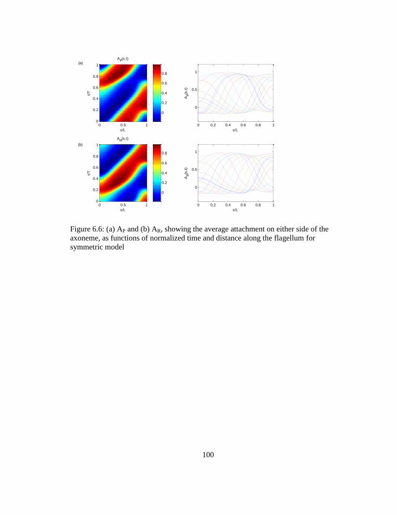
100

s/L

t/T

AP(s,t)

0 0.5 10

0.2

0.4

0.6

0.8

1

0

0.2

0.4

0.6

0.8

0 0.2 0.4 0.6 0.8 1

0

0.5

1

s/L

AP(s

,t)

s/L

t/T

AR(s,t)

0 0.5 10

0.2

0.4

0.6

0.8

1

0

0.2

0.4

0.6

0.8

0 0.2 0.4 0.6 0.8 1

0

0.5

1

s/L

AR(s

,t)

(a)

(b)

Figure 6.6: (a) AP and (b) AR, showing the average attachment on either side of the

axoneme, as functions of normalized time and distance along the flagellum for

symmetric model

101

s/L

t/T

TP(s,t)

0 0.5 10

0.2

0.4

0.6

0.8

1

-10

0

10

20

30

0 0.2 0.4 0.6 0.8 1-20

-10

0

10

20

30

40

s/L

TP(s

,t)

s/L

t/T

TR(s,t)

0 0.5 10

0.2

0.4

0.6

0.8

1

-10

0

10

20

30

0 0.2 0.4 0.6 0.8 1-20

-10

0

10

20

30

40

s/L

TR(s

,t)

(a)

(b)

Figure 6.7: (a) TP and (b) TR, showing the force contribution from the dynein arms on

either side of the axoneme, as functions of normalized time and distance along the

flagellum for symmetric model

6.3.2 Asymmetric Model Results

For the simulation of asymmetric motion, the force from dynein arms on the principal

side is assumed to be larger than that on the reverse side. In this model, dP is taken to

be twice the value of dR so 05.1 FFP and 075.0 FFR . The following figures

illustrate the results when this simulation is run for 0.2 sec.

102

0 0.2 0.4 0.6 0.8 1-2

-1

0

1

2

t/T

(s

,t)

Figure 6.8: Bend angle of the flagellum vs. normalized time during one complete cycle

from t=0.14 to t=0.20 sec.

-10 -5 0 5 10

-10

-5

0

5

10

x (m)

y (

m)

Figure 6.9: Shape history of the flagellum during 1 cycle from t=0.14 to t=0.2 sec,

shown every 0.005 sec for asymmetric model

103

0

0.5

1

0

0.5

1

-2

0

2

s/Lt/T

(s

,t)

0

0.5

1

0

0.5

1

-0.5

0

0.5

s/Lt/T

(s

,t)

0

0.5

1

0

0.5

1

-5

0

5

s/Lt/T

d

(s,t

)/dt

-1

0

1

2

-0.2

-0.1

0

0.1

0.2

-2

-1

0

1

2

3

(a) (b)

(c)

Figure 6.10: 3D surface plots showing (a) bend angle, (b) curvature, and (c) angular

velocity as a function of normalized time and distance along the flagellum during one

cycle for asymmetric model.

104

s/L

t/T

(s,t)

0 0.5 10

0.5

1

0 0.2 0.4 0.6 0.8 1-2

0

2

s/L

(s

,t)

s/L

t/T

(s,t)

0 0.5 10

0.5

1

0 0.2 0.4 0.6 0.8 1-0.5

0

0.5

s/L

(s

,t)

s/L

t/T

d(s,t)/dt

0 0.5 10

0.5

1

0 0.2 0.4 0.6 0.8 1-5

0

5

s/L

d

(s,t

)/dt

-1

0

1

2

-0.2

0

0.2

-2

0

2

(a)

(b)

(c)

Figure 6.11: (a) Bend angle, (b) curvature, and (c) angular velocity as functions of

normalized time and distance along the flagellum during one cycle from t=0.14 to

t=0.20 sec. for asymmetric model. The plots in the right column show these quantities

every 0.004 seconds.

105

0

0.5

1

0

0.5

1

0

0.5

1

s/Lt/T

AP(s

,t)

0

0.5

1

0

0.5

1

0

0.5

1

s/Lt/T

AR(s

,t)

0

0.5

1

0

0.5

1

-50

0

50

s/Lt/T

TP(s

,t)

0

0.5

1

0

0.5

1

-50

0

50

s/Lt/T

TR(s

,t)

-0.2

0

0.2

0.4

0.6

0.8

0

0.2

0.4

0.6

0.8

-10

0

10

20

30

40

50

-10

-5

0

5

10

15

20

(a) (b)

(d)(c)

Figure 6.12: 3D surface plots showing (a) AP, the average adhesion on the principal

side, (b) AR, the average adhesion on the reverse side, (c) TP, the force from the

attached dynein arms on the principal side, and (d) TR, the force from attached dynein

arms on the reverse side, as functions of normalized time and distance along the

flagellum for asymmetric model.

106

0 0.2 0.4 0.6 0.8 1

0

0.5

1

s/L

AP(s

,t)

0 0.2 0.4 0.6 0.8 1

0

0.5

1

s/L

AR(s

,t)

s/L

t/T

AP(s,t)

0 0.5 10

0.2

0.4

0.6

0.8

1

-0.2

0

0.2

0.4

0.6

0.8

s/L

t/T

AR(s,t)

0 0.5 10

0.2

0.4

0.6

0.8

1

0

0.2

0.4

0.6

0.8

(a)

(b)

Figure 6.13: (a) AP and (b) AR, showing the average attachment on either side of the

axoneme, as functions of normalized time and distance along the flagellum for

asymmetric model.

107

s/L

t/T

TP(s,t)

0 0.5 10

0.2

0.4

0.6

0.8

1

-10

0

10

20

30

40

50

0 0.2 0.4 0.6 0.8 1-20

0

20

40

60

s/L

TP(s

,t)

s/L

t/T

TR(s,t)

0 0.5 10

0.2

0.4

0.6

0.8

1

-10

-5

0

5

10

15

20

0 0.2 0.4 0.6 0.8 1-20

0

20

40

60

s/L

TR(s

,t)

(a)

(b)

Figure 6.14: (a) TP and (b) TR, showing the force contribution from the dynein arms on

either side of the axoneme, as functions of normalized time and distance along the

flagellum for asymmetric model.

6.4 Discussion

This model is useful because it combines the accurate equilibrium mechanics derived by

Hines and Blum (1978) with an excitable dynein mechanism to govern dynein

attachment and detachment. The adhesion mechanism in this model is superior to that

of the model described in Chapter 5.

By examining the shape histories of Figures 6.2 and 6.9, it can be seen that this model

produces more realistic simulations of the motion of the flagellum. In both the

symmetric and asymmetric simulations, there is much more bending than in the baseline

model of Chapter 5. The asymmetric model produces distinctions between the effective

stroke and the recovery stroke.

108

The adhesion mechanism in this model works much better than in the previous PDE

model. The goal of the adhesion mechanism is to start at the base and spread

attachments or detachments along the entire length of the flagellum. By examining

Figures 6.5-6.6 and 6.12-6.13, it can be seen that the adhesions do in fact vary from

zero to one for this model. At any point in time and at any distance along the flagellum,

the attachment on one side of the axoneme should be opposite of the attachments on the

other side of the axoneme. The figures of AP and AR show that this phenomenon occurs

for both the symmetric and asymmetric simulations.

For the symmetric model simulation, Figures 6.5 and 6.7 show that throughout the run,

the transverse force on the reverse side is equal and opposite to that on the principal

side. For the asymmetric simulation, the transverse force is negative and smaller than

the force on the principal side. This verifies that while one side is experiencing tension,

pulling the doublets further apart, the opposite side will experience compression,

pulling the doublets closer together. Comparing Figures 6.6 with 6.7 and 6.13 with

6.14, shows that when the adhesions on one side are increasing and approaching one,

the transverse force decreases. This verifies that the adhesion and transverse forces are

related such that when adhesion increases, the transverse force must decrease to allow

the interdoublet spacing to decrease.

While this model produces more realistic simulations of the motion of the flagellum and

accurately describes the adhesion and transverse force mechanisms, there is still ample

room for improvement. As in the previous model, at this stage, many of the parameter

values were chosen simply to see what was necessary to reproduce the observed

behavior. These parameters are chosen without significant biophysical justification.

For example, the diameter of the doublet is assumed to be 1 μm, for simplicity, but in

actuality the diameter of the doublet is closer to 0.037 μm [3]. Improvements to this

model include correcting the parameters to accurately represent the physical properties.

109

6.5 Conclusion

The model presented in this chapter combine the mechanics of Hines and Blum (1978)

with an excitable dynein mechanism. This model improves the adhesion mechanism

from the PDE model of Chapter 5 and more accurately reproduces the motion of the

flagellum. To improve this model, the underlying assumptions should be evaluated and

better estimates of physical parameters should be made.

110

7 Conclusions

Cilia and flagella are hair-like organelles that extend from many different types of cells.

While their primary responsibilities include moving fluid over cell surfaces, it is

becoming increasingly clear that these organelles have important sensory and motor

functions. The intraflagellar transport (IFT) system is needed to transport proteins from

the cell base throughout the length of the cilium. Mutations in the gene encoding

proteins of IFT cause defects to cilia and flagella that affect their motility and ability to

perform sensory functions. Functional failure of these organelles can lead to a wide

range of genetic and developmental disorders, such as PKD and situs inversus.

In this thesis, the 9+2 axoneme is examined; the axoneme consists of a central pair of

microtubules surrounded by a circular arrangement of nine doublets. The dynein arms

provide the active forces for bending while the nexin links and radial spokes provide

passive elastic resistance to bending. By modeling the flagellum as a thin beam of fixed

length, force and moment equilibrium are used to derive the governing mechanical

equations for such a structure. A shear growth analysis is included to illustrate how

shear displacement causes bending in a beam.

The first mathematical model studied in this thesis is the curvature-controlled model of

Hines and Blum (1978). In this model, the Gray-Hancock approximation is used in

conjunction with force and moment equilibrium to derive the governing equations of

motion for a flagellum. The radial are assumed to provide passive elastic resistance

proportional to shear angle and the force from the dynein arms is dependent on the

curvature of the flagellum. A stability analysis is conducted to determine the maximum

flexural stiffness and the minimum dynein feedback constant needed to produce

111

sustained oscillations. This model succeeds in producing continuous oscillations and

the mechanics are simple yet reliable. The main shortcoming of this model is the lack

of biophysical basis used in specifying the active force from the dynein arms.

A theoretical model that uses interdoublet spacing to control dynein arm activity is also

examined. The implementation of this model is based on the algorithm developed by

Lindemann (1994) in the "geometric clutch" model. This model separates the forces

from the active and passive elements into longitudinal and transverse components and

incorporates the adhesive effects of activated dynein arms. The transverse components

are believed to pull the doublets closer together. While this model produces realistic

simulations for the motion of cilia and flagella, much of the mechanics involved are

inconsistent.

The mechanics of Hines and Blum (1978), as discussed in Chapter 3, are combined with

the "geometric clutch" switching mechanism from Chapter 4 to produce a finite element

partial differential equation implementation of the interdoublet switching mechanism.

This model includes differential equations to represent an adhesion mechanism and

integral forces along the length of the flagellum. While this model does not produce

realistic behavior, it provides an illustration of how asymmetries in modeling

parameters affects the motion of the flagellum. The main problem with this model is

that the adhesion mechanism does not function properly.

To improve the first partial differential equation implementation described in Chapter 5,

an excitable dynein partial differential equation implementation is also used. The

mechanics of this model are the same as those in Chapter 5 but the adhesion mechanism

is modified to incorporate dynein excitement, recovery, and relaxation. This model also

has the benefit of using normalized forces. The simulation results from this model are

more realistic and the adhesion mechanism works properly. However, more research

should be done to develop a better biophysical basis for the modeling parameters.

112

Appendix A

Stability Analysis MATLAB Codes

Eb vs. k code

clear all tao=0.02; Cn=0.005; mo=130;

k1=-2:0.001:-0.000001; k2=0.000001:0.001:2; for n=1:length(k1) a(n)=tao*k1(n)^8/Cn; b(n)=0; c(n)=Cn/tao; d(n)=-mo^2*k1(n)^2; r=roots([a(n), b(n), c(n), d(n)]); Eb(1,n)=r(3,1); end plot(k1,Eb, 'linewidth', 1.75) hold on for n=1:length(k2) a(n)=tao*k2(n)^8/Cn; b(n)=0; c(n)=Cn/tao; d(n)=-mo^2*k2(n)^2; r=roots([a(n), b(n), c(n), d(n)]); Eb(1,n)=r(3,1); end plot(k2,Eb, 'linewidth', 1.75) hold off xlabel('k (\mum^[8])'), ylabel('E_{b} (pN \mum^{2})')

m0 vs. k code

k1=0.00001:0.001:2; k2=-2:0.001:-0.00001; Eb=30; Cn=0.005; tao=0.02; alpha=Eb/Cn*sqrt(Eb*Cn*tao); beta=1/tao*sqrt(Eb*Cn*tao); %alpha=10;

113

%beta=10; f1_1=alpha.*k1.^3; f1_2=alpha.*k2.^3; f2_1=beta.*k1.^(-1); f2_2=beta.*k2.^(-1); mo_1=f1_1+f2_1; mo_2=f1_2+f2_2; figure() plot(k1,mo_1, 'linewidth', 1.75), xlabel('k (\mum^{-

1})'),ylabel('m_{0} (pN \mum)') hold on plot(k2,mo_2, 'linewidth', 1.75) %hold on %plot(0,[-100:0.001:100],'k') %hold on %plot([-1:0.001:1],0,'k') hold off axis on axis([-1 1 -100 100])

114

Appendix B

Sample "Geometric Clutch" Model MATLAB Code

%Kate Nevin %Ver 7/14/08 %Lindemann geometric clutch model program

clear all

ROUTE=1;% intial and continuation routing PL=0; EX=0; N=0; Q=0; total=0; % plotting data from previous run % Below are the sizes and descriptions for some of the variable used % throughout the program % sx is a 32x1 matrix of x position % sy is a 32x1 matrix of y position % G is a 50x31 matrix for storage arrays for plotting a run -- NOT

USED % K is a 50x31 matrix for storage arrays for plotting a run -- NOT

USED % ang is a 31x1 mtrix of the angles for 30 segments 1 to 30 % sang is a 31x1 matrix of the shear angles % cur is a 31x1 matrix of the curvature values

% This program uses the following function %double find_angle(double, double, double) -- A function generated in

a seperate m-file to find the angle from slope and x,y positions;

ROUTE = 1; total = 0; EX = 0;

% Modeling parameters for 10 micron cilium COUPLING=.14; BRIDGEFORCE=1.2e-07; SNAP=.2; SWITCH_P=.06; SWITCH_R=.01; HISTER_P=33000.; HISTER_R=33000.; IE=1.0e-13; DIAM=1.0e-05; Z=3.33e-05; DRAG=0.028; GAIN=7000.;

115

ITS=.0001; STATE=1.0; BASE=1.0;

% Added line ang=zeros(31,1); %The below line specifies the initial angles %ang=sin(1:31);

%Load 30 angles for each of the segments along the cilium i = 1; for i=2:31 % ang(i)=0; %segment length Z is a modeling parameter as stated above sx(1)=0; sx(2)=0; sy(1)=0; sy(2)=0; for j=2:31 sx(j+1) = sx(j) +(Z * cos(ang(j))); sy(j+1) = sy(j) +(Z * sin(ang(j))); end cur(1)=0; cur(2)=0; sang(1)=0; sang(2)=0; for i=3:31 cur(i) = (ang(i)-ang(i-1)) / Z; %calculates the curvatures sang(i)=ang(i) - ang(2); end end % % end of load angles function

% For "find_angle" function file see find_angle.m; function used in

main % drag loop

% MAIN MODELING SUBROUTINE % This begins the modelling portion of the Geometric Clutch program

define local variables RPTS=0; DECAY_C=20000000000.0; TOTFORCE_R = .1; PANGL=0; LANGL=0; MAGN=0; XLEG=0; TORQUE=0; SUM_BP=0; SUM_BR=0;

ADJUST=0; DC=0.0; AVEBCORR=0; TOTCOR=0; DRAGTORQUE=0; DYDX=0; ARM=0; VECTX=0; VECTY=0;

PREVIOUS=0.0; HYPOT=0; DR=0; TF=0; PSI=0; SUMF=0; OLDDECAY=0; LONG_FORC_P=0;

LONG_FORC_R=0; DECAY=0.0; TVFR=0; TVFP=0; OLFORCE=0; TOTFORCE_P=0; CHOICE=0; FEEDBK=0;

NEWDECAY=0; PUSH=0.0; TRIGGER_P=0; TRIGGER_R=0; TRIGGEROOT_P=0; TRIGGEROOT_R=0; ADHESN_P=0;

ADHESN_R=0.0;

116

tfa=zeros(4,31); %t-force arrays 1 and 2 are long. and transverse

comp. while 3 and 4 are P and R t-force at each segment adh=zeros(2,32); %adhesion force storage forc=zeros(6,31); %longitudinal forces on the doublets dec=zeros(31,1); %DECAY values osx=zeros(32,1); %old x position data from previous iteration osy=zeros(32,1); %old y position data from previous iteration drag=zeros(31,1); %dragtorque values torq=zeros(31,1); %total torque passive and active equ=zeros(31,1); %equilibrium curvatures adj=zeros(31,1); %angle adjustments for feedback between iterations PL =0; EX = 0;

%Restate modeling parameters as done by Lindemann coupl=0.14; %Transfer factor TUG=1.2e-07; %Force per active dynein head (dyne) SNAP=0.2; %Elastic constant per nexin link, Ke SWITCH_P=.06; %Resting probability for P direction - BASE.P SWITCH_R=.01; %Resting probability for R direction - BASE.R HISTER_P=33000.; %Adhesion scaling factor for P direction HISTER_R=33000.; %Adhesion scaling factor for R direction IE=1.0e-13; DIAM=1.0e-05; %Functional diameter based on spacing between doublets

2-4 and doublets 7-9 (cm) Z=3.33e-05; %Secment length (cm) D=0.028; %Drag coefficient GAIN=7000.; %T-force scaling factor ITS=.0001; STATE=1.0; BASE=1.0; %End of local variables

A=1;

% ---THE GEOMETRIC CLUTCH MODEL---" ; num_its=input('Choose the number of iterations between 100 and 1000') N=num_its;

% Define the total output arrays SX = zeros(N+1,32); SY = zeros(N+1,32);

for n=1:(N+1) %MAIN ITERATION LOOP FOR MODELING % FIND T-FORCE sang(2)=0; for j=2:31 HYPOT =sqrt(((sang(j)*DIAM)*(sang(j)* DIAM))+.0000033^2); % DR is the stretch of the nexin link, DR=hypot-resting length

of % nexin link, sang(j)*DIAM=shear displacement due to sliding % between doubles 2-4 or 7-9, ignoring 3 or 8 DR=HYPOT - .0000033;

117

TF = SNAP * DR; %Force from stretching elastic components, Fe if (sang(j)==0) sang(j)=.000001; end PSI=abs(atan(.0000033/(sang(j)*DIAM))); tfa(1,j)=TF * cos(PSI) * (sang(j)/abs(sang(j))); %Longitudinal

component of passive force from stretching nexin links at each

segment, Fl(n). Eqn. 7, can be + or - depending on how spacing

changes tfa(2,j)=TF * sin(PSI); %Transverse component of passive force

from stretching nexin links at each segment, Ft(n). Eqn. 6, always +

since spacing always decreases end for l=2:31 %summation loop for passive force SUMF=0; for k=2:31 SUMF=SUMF+tfa(1,k); end forc(4,l)=SUMF; %Cumulative long. force on each segment from

stretching nexin links end

%FIND ACTIVE FORCES USING THE T-FORCE MECHANISM if STATE~=0 for l=2:30 %loop for bridge control LONG_FORC_P = forc(4,l)+ forc(5,l)*(1.0 - coupl) + coupl *

forc(6,l); %Total long. force at each segment on P side from passive

and active elements, revised parenthesis in Eqn. 10a LONG_FORC_R = forc(4,l) + forc(6,l)*(1.0 - coupl) + coupl

* forc(5,l); %Total long. force at each segment on R side from passive

and active elements, revised parenthesis in Eqn. 10b TVFP =tfa(2,l) + Z*cur(l+1)*LONG_FORC_P; %Eqn. 10a

without summation TVFR =tfa(2,l) + Z*cur(l+1)*LONG_FORC_R; %Eqn. 10b

withouth summation tfa(3,l) = TVFP; %Stores the total t-force in the

principal bend direction at each segment, Eqn. 10a (local+global t-

force) tfa(4,l) = TVFR; %Stores the total t-force in the reverse

bend direction at each segement, Eqn. 10b TRIGGEROOT_P = SWITCH_P + (TVFP * GAIN); %Adjust base

probability by accounting for t-force to get active probability of

attachment for P, Eqn. 11 TRIGGEROOT_R = SWITCH_R + (TVFR * GAIN); %Active

probability of attachment for R, Eqn. 11 TRIGGER_R = TRIGGEROOT_R + adh(2,l) +.5 * adh(2,l-1)+ .5 *

adh(2,l+1); %Adjust active probability for attachment by incorporating

previous iteration's adhesive force effects to get dynamic probability

for R, Eqn. 14 if (TRIGGER_R<0.0) TRIGGER_R = 0.0; end

118

TRIGGER_P = TRIGGEROOT_P + adh(1,l) +.5 * adh(1,l-1)+ .5 *

adh(1,l+1); %Dynamic probability for P, Eqn. 14 if (TRIGGER_P<=0.0) TRIGGER_P = 0.0; end CHOICE = abs(TOTFORCE_R); if (abs(TOTFORCE_P)>=abs(TOTFORCE_R)) CHOICE = abs(TOTFORCE_P); end OLFORCE = 1.0; COUNTER = 0; while ((abs((CHOICE/OLFORCE)-1))>.1) %Loop ends when there

is less than a 10% change in total dynein bridge attachment COUNTER=COUNTER+1; if COUNTER>150 break end OLFORCE=CHOICE; TOTFORCE_P=0.0; TOTFORCE_R=0.0; for BRIDGE=1:floor(4000000.0*Z) %Dynein bridge

switching algorithm R = rand; BRVAL = R; if (BRVAL<TRIGGER_P) %Compare random number to

probability of attachment to determine if bridge attachment occurs TOTFORCE_P=TOTFORCE_P+TUG; %For each dynein

head that attaches on the principal side, add the force for one

additional head to the active bridge force end R = rand; BRVAL = R; %Not sure if this is right because TOTFORCE_R is 0

a %lot if (BRVAL<abs(TRIGGER_R)) TOTFORCE_R=TOTFORCE_R-TUG; %For each dynein

head that detaches on the principal side, subtract that force from the

active bridge force end end %Adhesive contribution to bridge switching probability ADHESN_P = abs(TOTFORCE_P) * ((1.0 - TRIGGEROOT_P) *

HISTER_P); %Equation 12 ADHESN_R = abs(TOTFORCE_R) * ((1.0 - TRIGGEROOT_R) *

HISTER_R); %Equation 12 %Adjust adhesive forces for transaxonemal force

transfer %and store for each element adh(1,l) = ADHESN_P - coupl * ADHESN_R; %Equation 13a adh(2,l) = ADHESN_R - coupl * ADHESN_P; %Equation 13b %Reevaluate dynamic probability after adjusting

adhesive %contribution

119

TRIGGER_R = TRIGGEROOT_R + adh(2,l) +.5 * adh(2,l-1)+

.5 * adh(2,l+1); %Dynamic probability with adhesive force correction

from this iteration, Equation 14 TRIGGER_P = TRIGGEROOT_P + adh(1,l) +.5 * adh(1,l-1)+

.5 * adh(1,l+1); %Equation 14 forc(2,l) = TOTFORCE_P; %Long. force at each segment

from activated bridges in P direction, Fp(i) forc(3,l) = TOTFORCE_R; %Long. force at each segment

from activated bridges in R direction, Fr(i) CHOICE = abs(TOTFORCE_R); if (abs(TOTFORCE_P)>=abs(TOTFORCE_R)) CHOICE=abs(TOTFORCE_P); end if (OLFORCE == 0.0) OLFORCE=.0000001; end if (CHOICE == 0) CHOICE = OLFORCE; end end end %End of bridge control loop for i=2:31 %sum up forces from current position to tip SUM_BP=0; SUM_BR=0; for j=i:31 %Cumulative istal sum of long. force at each

segment SUM_BP = SUM_BP+forc(2,j); SUM_BR = SUM_BR+forc(3,j); end forc(5,i) = SUM_BP; %Stores cumulative distal sum of total

long. force contributed by activated bridges in P; Fp forc(6,i) = SUM_BR; %Stores cumulative distal sum of total

long. force contributed by activated bridges in R; Fr end %End of active force calculation end % END OF IF STATE~=0 CONDITION

%PASSIVE for l=2:31 %calculation of torques and equil curvatures forc(1,l) = 2*forc(4,l) + forc(5,l) + forc(6,l); %Total long.

force at each segment for top or bottom half, Eqn. 4a and 1b torq(l)= forc(1,l)* DIAM; %instantaneous torque equ(l)=-torq(l)/IE; %Equilibrium curvature OLDDECAY = dec(l); NEWDECAY = .6/(1+abs(drag(l) * DECAY_C)); if (n==1 && ROUTE==1) NEWDECAY=.06; end if (n==2 && ROUTE==1) NEWDECAY=.04; end if (n==3 && ROUTE==1) NEWDECAY=.02; end

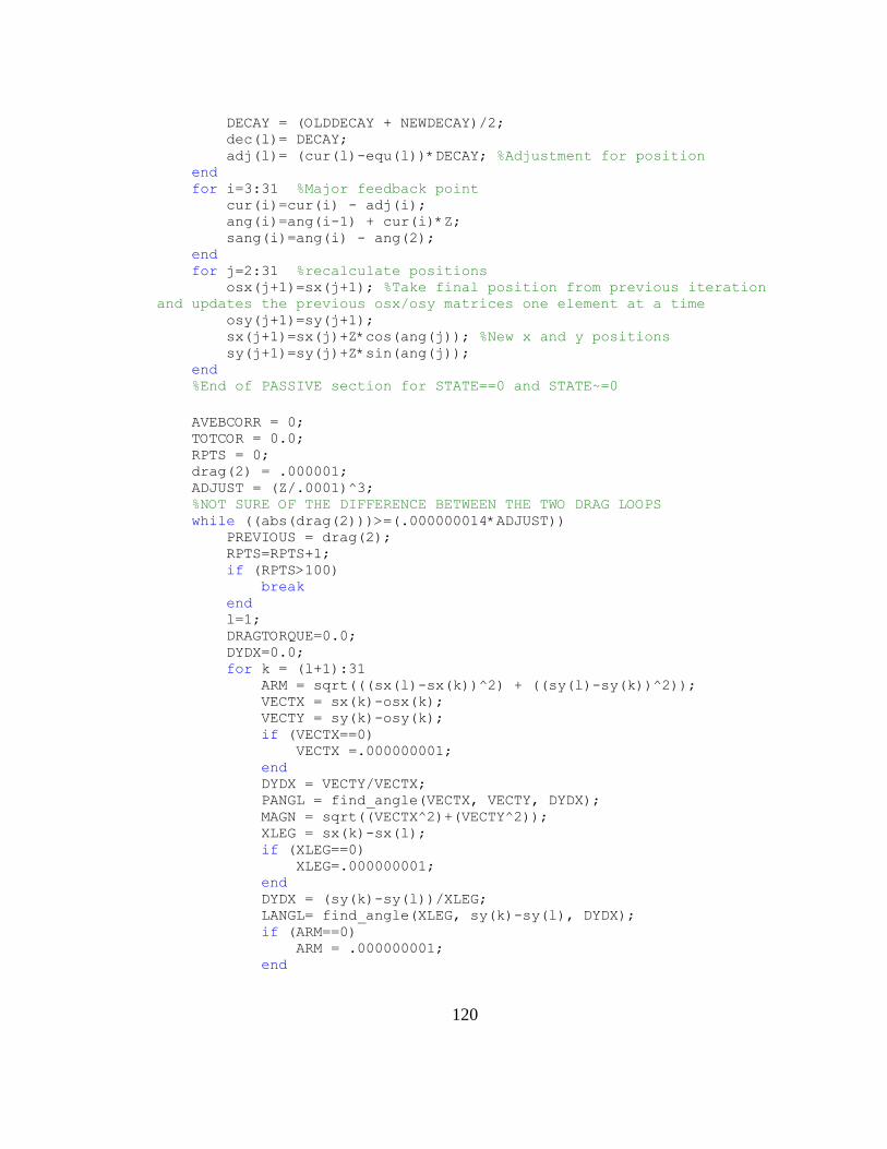
120

DECAY = (OLDDECAY + NEWDECAY)/2; dec(l)= DECAY; adj(l)= (cur(l)-equ(l))*DECAY; %Adjustment for position end for i=3:31 %Major feedback point cur(i)=cur(i) - adj(i); ang(i)=ang(i-1) + cur(i)*Z; sang(i)=ang(i) - ang(2); end for j=2:31 %recalculate positions osx(j+1)=sx(j+1); %Take final position from previous iteration

and updates the previous osx/osy matrices one element at a time osy(j+1)=sy(j+1); sx(j+1)=sx(j)+Z*cos(ang(j)); %New x and y positions sy(j+1)=sy(j)+Z*sin(ang(j)); end %End of PASSIVE section for STATE==0 and STATE~=0

AVEBCORR = 0; TOTCOR = 0.0; RPTS = 0; drag(2) = .000001; ADJUST = (Z/.0001)^3; %NOT SURE OF THE DIFFERENCE BETWEEN THE TWO DRAG LOOPS while ((abs(drag(2)))>=(.000000014*ADJUST)) PREVIOUS = drag(2); RPTS=RPTS+1; if (RPTS>100) break end l=1; DRAGTORQUE=0.0; DYDX=0.0; for k = (l+1):31 ARM = sqrt(((sx(l)-sx(k))^2) + ((sy(l)-sy(k))^2)); VECTX = sx(k)-osx(k); VECTY = sy(k)-osy(k); if (VECTX==0) VECTX =.000000001; end DYDX = VECTY/VECTX; PANGL = find_angle(VECTX, VECTY, DYDX); MAGN = sqrt((VECTX^2)+(VECTY^2)); XLEG = sx(k)-sx(l); if (XLEG==0) XLEG=.000000001; end DYDX = (sy(k)-sy(l))/XLEG; LANGL= find_angle(XLEG, sy(k)-sy(l), DYDX); if (ARM==0) ARM = .000000001; end

121

TORQUE = ARM * D * Z *((MAGN * sin(PANGL-LANGL))/ITS);

%individual contributions DRAGTORQUE = DRAGTORQUE+TORQUE; %running sum of

individual contrib. end drag(2)=DRAGTORQUE; %current value of drag at segment 1 the

base FEEDBK = 6000/(D*ADJUST); PUSH = drag(2)*FEEDBK; AVEBCORR = -PUSH; TOTCOR= TOTCOR+AVEBCORR; for j=2:31 ang(j)= ang(j)+ AVEBCORR; sx(j+1) = sx(j) + Z*cos(ang(j)); sy(j+1) = sy(j) + Z*sin(ang(j)); end if (RPTS>1 && (drag(2)*PREVIOUS)<0 ) drag(2)=0.0; end end for j=2:31 ang(j)=ang(j)-TOTCOR*BASE; sx(j+1)=sx(j)+Z*cos(ang(j)); sy(j+1)=sy(j)+Z*sin(ang(j)); end if (BASE==1.0) %Main drag loop in Lindemann paper for l=2:31 DRAGTORQUE=0.0; DYDX=0.0; for k = l+1:32 ARM = sqrt(((sx(l)-sx(k))^2) + ((sy(l)-sy(k))^2)); VECTX = sx(k)-osx(k); VECTY = sy(k)-osy(k); if (VECTX==0) VECTX =.000000001; end DYDX = VECTY/VECTX; PANGL = find_angle(VECTX, VECTY, DYDX); MAGN = sqrt((VECTX^2)+(VECTY^2)); XLEG = sx(k)-sx(l); if (XLEG==0) XLEG=.000000001; end DYDX = (sy(k)-sy(l))/XLEG; LANGL= find_angle(XLEG, sy(k)-sy(l), DYDX); if (ARM==0) ARM = .000000001; end DC = .5*D+(.5 * D * abs(sin(PANGL-ang(k-1)))); TORQUE = ARM * DC * Z *((MAGN * sin(PANGL-

LANGL))/ITS); %individual contributions DRAGTORQUE = DRAGTORQUE+TORQUE; %running sum of

individual contrib. end

122

drag(l)=DRAGTORQUE; %store them in the drag array end end total=total+1; % Store position at this time point SX(n,:) = sx; SY(n,:) = sy; n; dx=diff(sx); dy=diff(sy); ds=sqrt(dx.^2+dy.^2); Sn(n+1)=sum(ds); end % End of main iteration loop %ROUTE=2;

%Now try to animate motion of cilium figure() for n=1:(N+1) plot(SX(n,:),SY(n,:)), axis([-30*Z 30*Z -30*Z 30*Z]),

axis('square'), mov1(:,n)=getframe; end % figure(1) % plot(SX,SY) %Plots the shape of the cilium at each segment figure() plot(SX(10:75:N+1,:)',SY(10:75:N+1,:)'), xlabel('X (cm)'), ylabel('Y

(cm)'), axis([-0.00025 0.0011 -0.00084 0.00053]), axis('equal') %Plots

time history of cilium at each iteration % figure() % plot(0:(N+1),Sn) % figure() % plot(SX(1:100:N,:)',SY(1:100:N,:)'), axis([-30*Z 30*Z -30*Z 30*Z]),

axis('square') figure() plot(Sn), axis([0 500 0.7e-3 1.3e-3]) x_std=mean(std(SX')); y_std=mean(std(SY')); min_amp=min(min(SY')); max_amp=max(max(SY')); stats=[x_std, y_std, min_amp, max_amp]; %Use the following commands to add the statistical data and SX and SY

infomation to an excel %spreadsheet d=(stats)'; xlswrite('sx_sy_stat_data.xls', d, 'Orig drag & vary coeff', 'k2')

123

Appendix C

Code used to show waveforms and create movies

% change the next line to reflect the length of the domain Lx = 12; % domain size Nx = 100; % # space points dx = Lx/Nx; % space discretization for visualization XX=0:dx:Lx; % space points

dt = 0.001; % COARSE time step for visualization %Ti = 0.1; % start time Ti=0; Tper=0.057; Tf = 0.2; % final time Nt = (Tf-Ti)/dt; % number of time plots nskip = 10; % skip number for snapshots

tt = Ti:dt:Tf; % time vector

[alpha,Fn,Ft,]=postinterp(fem,'alpha','Fn','Ft',XX,'T',tt);

scal = 1;

% now step through time and make subplots % assuming a 4x4 grid of subplots

figure(1) for n=1:Nt,

% extract solution at given points in space and time

% wave form x=cumtrapz(XX,cos(alpha(n,:))); y=cumtrapz(XX,sin(alpha(n,:))); figure(1) plot(x,y,'linewidth',1.5) axis([-Lx Lx -Lx Lx]), axis('square') xlabel('x ({\mu}m)') ylabel('y ({\mu}m)') MOV(:,n)=getframe;

end;

124

x=cumtrapz(XX',cos(alpha')); y=cumtrapz(XX',sin(alpha'));

% x, y, and alpha are plotted every 20 iterations starting at the 5th % iteration. This corresponds to starting at t=0.004 sec and ending

at % t=0.184 sec showing the values every 0.02 sec

figure(2) plot(x(:,5:20:end),y(:,5:20:end)) axis([-Lx Lx -Lx Lx]); axis('square'); xlabel('x (\mum)'), ylabel('y (\mum)') %Normalized length = s_L s_L=XX/Lx; figure(3) plot(s_L, alpha(5:20:end,:)) axis([0 1 -2 2]) xlabel('s/L'), ylabel('\alpha (rad)')

figure(4), plot(tt,alpha(:,Nx/2)); xlabel('t (sec)') ylabel('{\alpha} (rad)')

figure(1), hold off % figure(2), hold off % figure(3), hold off

T0 = 0; % start time Tper = 0.057; % period (empirically determined) Tf = 0.2; % end time dt = 0.001; Nt=Tf/dt;

Lx=12; Nx=100; dx=Lx/Nx; XX=0:dx:Lx; % space points tt=(Tf-Tper):dt:Tf; %time points

% extract data rfom comsol [alpha,Fn,Ft,AP,AR,TP,TR]=postinterp(fem,'alpha','Fn','Ft','AP','AR','

TP','TR',XX,'T',tt);

% time series of angle at midpoint figure(5) subplot(2,2,1) plot((tt-tt(1))/Tper,alpha(:,50)), %axis([tt(1)/Tper tt(end)/Tper -0.2 0.6]), axis square

125

xlabel('t/T'), ylabel('{\alpha}(s,t)')

% MAKE ANGLE, CURVATURE, ANGULAR VELOCITY PLOTS % First, compute curvature and angular velocity [curv,angvel]=gradient(alpha,0.3,.1); figure(6) subplot(3,2,1) imagesc(XX/Lx,(tt-tt(1))/Tper,alpha) h=gca; set(h,'ydir','normal'); % flip y-axis orientation on

image xlabel('s/L'), ylabel('t/T'), title('{\alpha}(s,t)') colorbar('eastoutside')

subplot(3,2,2) plot(XX/Lx,alpha(1:4:end,:)') xlabel('s/L'), ylabel('{\alpha}(s,t)')

subplot(3,2,3) imagesc(XX/Lx,(tt-tt(1))/Tper,curv) h=gca; set(h,'ydir','normal'); xlabel('s/L'), ylabel('t/T'), title('{\kappa}(s,t)') colorbar('eastoutside')

subplot(3,2,4) plot(XX/Lx,curv(1:4:end,:)') xlabel('s/L'), ylabel('{\kappa}(s,t)')

subplot(3,2,5) imagesc(XX/Lx,(tt-tt(1))/Tper,angvel) h=gca; set(h,'ydir','normal'); xlabel('s/L'), ylabel('t/T'), title('d{\alpha}(s,t)/dt') colorbar('eastoutside')

subplot(3,2,6) plot(XX/Lx,angvel(1:4:end,:)') xlabel('s/L'), ylabel('d{\alpha}(s,t)/dt')

% SURFACE PLOT EXAMPLES figure(7) subplot(2,2,1) surf(XX/Lx,(tt-tt(1))/Tper,alpha) shading interp view(-35,65) xlabel('s/L'), ylabel('t/T'), zlabel('{\alpha}(s,t)') colorbar('eastoutside')

subplot(2,2,2) surf(XX/Lx,(tt-tt(1))/Tper,curv) shading interp view(-35,65) xlabel('s/L'), ylabel('t/T'), zlabel('{\kappa}(s,t)') colorbar('eastoutside')

126

subplot(2,2,3) surf(XX/Lx,(tt-tt(1))/Tper,angvel) shading interp view(-35,65) xlabel('s/L'), ylabel('t/T'), zlabel('d{\alpha}(s,t)/dt') colorbar('eastoutside')

% NOW MAKE 3D SURFACE PLOTS AND LINE PLOTS OF AP, AR, TP, AND TR LIKE

WE % DID FOR THE BEND ANGLE, CURVATURE, AND ANGULAR VELOCITY figure(8) subplot(2,2,1) surf(XX/Lx,(tt-tt(1))/Tper,AP) shading interp view(-35,65) xlabel('s/L'), ylabel('t/T'), zlabel('A_P(s,t)'), axis([0 1 0 1 -0.2

1]) colorbar('eastoutside')

subplot(2,2,2) surf(XX/Lx,(tt-tt(1))/Tper,AR) shading interp view(-35,65) xlabel('s/L'), ylabel('t/T'), zlabel('A_R(s,t)'), axis([0 1 0 1 -0.2

1]) colorbar('eastoutside')

subplot(2,2,3) surf(XX/Lx,(tt-tt(1))/Tper,TP) shading interp view(-35,65) xlabel('s/L'), ylabel('t/T'), zlabel('T_P(s,t)') colorbar('eastoutside')

subplot(2,2,4) surf(XX/Lx,(tt-tt(1))/Tper,TR) shading interp view(-35,65) xlabel('s/L'), ylabel('t/T'), zlabel('T_R(s,t)') colorbar('eastoutside')

figure(9) subplot(2,2,1) imagesc(XX/Lx,(tt-tt(1))/Tper,AP) h=gca; set(h,'ydir','normal'); % flip y-axis orientation on

image xlabel('s/L'), ylabel('t/T'), title('A_P(s,t)') colorbar('eastoutside')

subplot(2,2,2)

127

plot(XX/Lx,AP(1:4:end,:)') xlabel('s/L'), ylabel('A_P(s,t)'), axis([0 1 -0.4 1.2])

subplot(2,2,3) imagesc(XX/Lx,(tt-tt(1))/Tper,AR) h=gca; set(h,'ydir','normal'); % flip y-axis orientation on

image xlabel('s/L'), ylabel('t/T'), title('A_R(s,t)') colorbar('eastoutside')

subplot(2,2,4) plot(XX/Lx,AR(1:4:end,:)') xlabel('s/L'), ylabel('A_R(s,t)'), axis([0 1 -0.4 1.2])

figure(10) subplot(2,2,1) imagesc(XX/Lx,(tt-tt(1))/Tper, TP) h=gca; set(h,'ydir','normal'); % flip y-axis orientation on

image xlabel('s/L'), ylabel('t/T'), title('T_P(s,t)') colorbar('eastoutside')

subplot(2,2,2) plot(XX/Lx,TP(1:4:end,:)') xlabel('s/L'), ylabel('T_P(s,t)')

subplot(2,2,3) imagesc(XX/Lx,(tt-tt(1))/Tper,TR) h=gca; set(h,'ydir','normal'); % flip y-axis orientation on

image xlabel('s/L'), ylabel('t/T'), title('T_R(s,t)') colorbar('eastoutside')

subplot(2,2,4) plot(XX/Lx,TR(1:4:end,:)') xlabel('s/L'), ylabel('T_R(s,t)')

128

References

1. Ainsworth, C., Cilia: tails of the unexpected, in Nature. 2007. p. 638-641.

2. Badano, J.L., et al., The ciliopathies: an emerging class of human genetic

disorders. Annu Rev Genomics Hum Genet, 2006. 7: p. 125-48.

3. Blum, J.J.a.L., J., Biophysics of flagellar motility. Annual Review of Biophysics

and Bioengineering, 1973. 2: p. 181-219.

4. Bray, D., in Cell Movements. 1992, Garland Pub.: New York.

5. Brokaw, C.J., Bend propagation by a sliding filament model for flagella. J Exp

Biol, 1971. 55(2): p. 289-304.

6. Ferkol, T. 2008, Washington University School of Medicine: St. Louis, MO. p.

22-29.

7. Fliegauf, M., T. Benzing, and H. Omran, When cilia go bad: cilia defects and

ciliopathies. 2007. 8(11): p. 880-893.

8. Fung, Y.C., in Biomechanics: motion, flow, stress, and growth. 1990, Springer:

New York. p. 124-141.

9. Hines, M. and J.J. Blum, Bend propagation in flagella. I. Derivation of

equations of motion and their simulation. Biophys J, 1978. 23(1): p. 41-57.

10. Humphrey, J.D., Cardiovascular solid mechanics: cells, tissues, and organs.

2002, New York: Springer-Verlag.

11. Lighthill, J., Flagellar hydrodynamics. SIAM Review, 1976. 18(2): p. 161-230.

12. Lindemann, C.B., A "geometric clutch" hypothesis to explain oscillations of the

axoneme of cilia and flagella. J Theor Biol, 1994. 168: p. 175-189.

13. Lindemann, C.B., A model of flagellar and ciliary functioning which uses the

forces transverse to the axoneme as the regulator of dynein activation. Cell

Motility and the Cytoskeleton, 1994. 29(2): p. 141-154.

129

14. Lindemann, C.B., Geometric clutch model version 3: the role of the inner and

outer arm dyneins in the ciliary beat. Cell Motility and the Cytoskeleton, 2002.

52(4): p. 242-254.

15. Murase, M., The dynamics of cellular motility. 1992, New York: J. Wiley &

Sons.

16. Sale, W.S. and P. Satir, Direction of active sliding of microtubules in

Tetrahymena cilia. Proc. Natl. Acad. Sci. USA, 1977. 74(5): p. 2045-2049.

17. Vogel, G., Betting on cilia, in Science. 2005. p. 216-218.

130

Vita

Kate Elizabeth Nevin

Date of Birth September 14, 1986

Place of Birth Manhasset, New York

Degrees B.S. Mechanical Engineering, May 2009

M.S. Mechanical Engineering, May 2009

Professional Society of Women Engineers

Societies Tau Beta Pi

Pi Tau Sigma

May 2009

131

Short Title: Modeling Cilia Mechanics & Control, Nevin, M.S. 2009