i

PORTFOLIO DIVERSIFICATION IN MALAYSIAN STOCK

MARKET

ADAM KOK KA HOH

HO CHEE WEI

LEE YIP CHUN

NGOI KOK HOU

TEH XUE SHUN

BACHELOR OF FINANCE (HONS)

UNIVERSITI TUNKU ABDUL RAHMAN

FACULTY OF ACCOUNTANCY AND MANAGEMENT

DEPARTMENT OF ECONOMICS

APRIL 2011

i

PORTFOLIO DIVERSIFICATION IN MALAYSIAN

STOCK MARKET

BY

ADAM KOK KA HOH

HO CHEE WEI

LEE YIP CHUN

NGOI KOK HOU

TEH XUE SHUN

A research project submitted in partial fulfillment of the

requirement for the degree of

BACHELOR OF FINANCE (HONS)

UNIVERSITI TUNKU ABDUL RAHMAN

FACULTY OF ACCOUNTANCY AND MANAGEMENT

DEPARTMENT OF ECONOMICS

APRIL 2011

ii

Copyright @ 2011

ALL RIGHTS RESERVED. No part of this paper may be reproduced, stored

in a retrieval system, or transmitted in any form or by any means, graphic,

electronic, mechanical, photocopying, recording, scanning, or otherwise,

without the prior consent of the authors.

iii

DECLARATION

We hereby declare that:

(1) This UBFZ 3026 Research Project is the end result of our own work and

that due acknowledgement has been given in the references to ALL sources

of information be they printed, electronic, or personal.

(2) No portion of this research project has been submitted in support of any

application for any other degree or qualification of this or any other university,

or other institutes of learning.

(3) Equal contribution has been made by each group member in completing

the research project.

(4) The word count of this research report is ___18,675_________________.

Name of Student: Student ID: Signature:

1. ADAM KOK KA HOH 09UKB08654 _____________

2. HO CHEE WEI 09UKB08861 _____________

3. LEE YIP CHUN 09UKB08801 _____________

4. NGOI KOK HOU 09UKB08860 _____________

5. TEH XUE SHUN 09UKB06708 _____________

Date: _____________

iv

ACKNOWLEDGEMENT

First of all, I am heartily thankful to our supervisor, Mr. Raymond Ling Leh Bin,

whose encouragement, guidance and support from the initial to the final level

enabled me and my fellow thesis group members to develop an

understanding of the subject. This thesis would be successful complete

without the proper guidance as well as his patience and steadfast

encouragement to complete this study by giving valuable recommendations

throughout this project. Although there maybe some difficulties in doing this

research, but we were advised and taught patiently until we knew the proper

direction to follow up with this research . He is giving the best effort he could

to teach us until we understand what we supposed to do with the project work.

I would also like to thank our second examiner, Ms. Tan Kok Eng for giving

me valuable suggestions and also correcting the mistakes done in our in the

course of our research. With the valuable insights in the relevance of the

study she shared to us my group would able to correct and improve our

research.

Last but not least, it is a pleasure to thank those who made this thesis

possible especially my thesis group members who were doing this project

with me and sharing our ideas. They were helpful that when we combined

and discussed together, we had this task done. This dissertation would not

have been possible without the guidance and the help of my members who in

one way or another contributed and extended their valuable assistance in the

preparation and completion of this study together with their unselfish and

unfailing support.

Lee Yip Chun,

Thesis group leader

v

TABLE OF CONTENTS

Title page i

Copyright Page ii

Declaration iii

Acknowledgement iv

Table of Contents v

List of Tables viii

List of Figures ix

Abstract x

CHAPTER 1 INTRODUCTION

1.1 Introduction of research project 1

1.2 Background of the study

1.2.1 Definition of Diversification 1

1.2.2 Types of Diversification 2

1.2.3 Strategies of Diversification 3

1.2.4 Factors that affecting portfolio diversification 4

1.3 Research Problems 6

1.4 Research Objectives 7

1.5 Significant of Study 8

CHAPTER 2 LITERATURE REVIEW

2.1 Review of Literature 9

2.2 Retrospective Part (before year 2000) 9

2.3 Modern Part (after year 2000) 11

2.4 Malaysia 13

2.5 Gaps on the Literature 14

2.6 Summary of Literature Review 15

vi

CHAPTER 3 METHODOLOGY

3.1 Data 17

3.2 Model Design

3.2.1 Descriptive Statistic

3.2.1.1 Arithmetic Mean (AM) 19

3.2.1.2 Standard Deviation 20

3.2.1.3 R-squared as Diversification Measure 20

3.2.2 Risk-adjusted Performance Indices

3.2.2.1 Sharpe Ratio 21

3.2.2.2 Treynor Ratio 22

3.2.2.3 Jensen’s Index 23

3.2.3 Generalized Autoregressive Conditional

Heteroscedasticity model (GARCH) 25

3.2.4 Unit Root Test

3.2.4.1 Augmented Dickey-Fuller test (ADF) 27

3.2.4.2 Non-parametric Phillips-Perron

test (PP) 28

3.2.4.3 Kwiatkowski et al. test (KPSS) 29

3.2.5 VAR Lag Order Selection Criteria

3.2.5.1 Akaike’s Information Criterion (AIC) 30

3.2.5.2 Schwarz’s Information Criterion (SIC) 30

3.2.6 Johansen and Juselius Cointegration Test 30

3.3 Hypothesis 32

3.4 Summary of Methodologies 33

CHAPTER 4 DATA RESULTS 35

vii

CHAPTER 5 INTERPRETATION OF RESULTS

5.1 Risk-Adjusted Performance Indices

(Sharpe, Treynor and Jensen’s index) 53

5.2 GARCH Model

5.2.1 ARCH Output (significance of model) 55

5.2.2 Garch Graph 56

5.2.3 GARCH Output 56

5.2.4 GARCH Forecasting 61

5.3 R-squared Diversification Measure 62

5.4 Unit Root Test 63

5.5 Johansen and Juselius Cointegration Test 63

5.5 R-squared for Correlation and Cointegration

based portfolio 64

CHAPTER 6 CONCLUSION AND RECOMMENDATIONS

6.1 Conclusions 65

6.2 Limitations 68

6.3 Recommendations 70

References 74

viii

LIST OF TABLES

Table 1: Ratio part for 13 years period 35

Table 2: Ratio part for crisis period 35

Table 3: ARCH coefficients, F-statistics and Obs*R-squared

for 13 years period 36

Table 4: ARCH coefficients, F-statistics and Obs*R-squared

for crisis period 37

Table 5: GARCH model coefficient (13 years period) 38

Table 6: GARCH model coefficient (crisis period) 39

Table 7: GARCH forecasting (by using 13 years period data) 42

Table 8: GARCH forecasting (by using crisis period data) 44

Table 9: R-squared for each number of stocks 46

Table 10: Stationary Tests on the 15 Stocks within the

Cointegration based Portfolio at level 47

Table 11: Critical values for the unit root tests 47

Table 12: The VAR Lag Order Selection Criteria 48

Table 13: Johansen and Juselius Cointegration Test Results 48

Table 14: R-squared for Correlation and Cointegration based portfolio 50

ix

LIST OF FIGURES

Figure 1: GARCH graph for all types of portfolio (13 years period) 40

Figure 2: GARCH graph for all types of portfolio (crisis period) 41

Figure 3: The Stock Prices Movement within the Correlation

based Portfolio in the long run 50

Figure 4: The Stock Prices Movement within the Cointegration

based Portfolio in the long run 51

Figure 5: The Stock Prices Movement within the Correlation

based Portfolio in the crisis period 51

Figure 6: The Stock Prices Movement within the Cointegration

based Portfolio in the crisis period 52

x

ABSTRACT

The debate against the performance between Active portfolio strategy and

Passive portfolio strategy has been existed for decade. As an investor, the

relationship between risk and return plays an important role in constructing

portfolio. Active portfolio holder diversifies their portfolio by actively trading

and managing portfolio, while passive portfolio holder constructs their portfolio

and hold for their desire tenure. Investors are also interesting regarding which

strategy perform the best during long term and crisis period. Besides, the

reliability of correlation coefficient method that is widely used in constructing

Active portfolio has been questioned by many researchers. In this research,

all the above statement will bring into Malaysian stock market perspective.

The ratios used to measure the risks and returns are Sharpe Ratio, Jensen

Index, and Treynor Index. The test used in this research includes GARCH,

Unit root and cointegration. This research has included 13 years period of

daily data for long run performance comparison, and 2007 crisis period for the

performance comparison within crisis period. The findings obtained from this

research showed that during both the long run and crisis period Active

portfolio strategy does outperformed Passive portfolio strategy. Empirical

results also showed that Malaysian stock market is not efficient compared to

developed countries as it does not provide significant diversification benefits

when simply adding more stocks in a portfolio. While by comparing the

performance between correlations based portfolio and cointegration based

portfolio, the cointegration based portfolio does outperformed the correlation

based portfolio.

1

CHAPTER 1.0 INTRODUCTION

1.1 Introduction of Research Project

The debate between passive diversification strategy and active

diversification strategy over which one is a better strategy has existed long

in the stock market. Thus, in this paper, this research aimed at finding out

which strategy is more appropriate to be used in Malaysian stock market

over the long run and during the crisis as well as determining the level of

diversification that can be achieved in Malaysian stock market by randomly

selecting a number of stocks ranging from 10 to a maximum of 100 stocks.

Besides that, this research will also examine the construction of portfolio

based on correlation and cointegration analysis.

In chapter 1, this research will briefly discuss the background of the study.

The background started with stock market theory. Then, it is narrowed

down to the area of diversification, which includes the types and strategies

of diversification, evidence on diversification, how combination of stocks

can be done, and finally the factors affecting the portfolio diversification.

The background of the study is followed by the problems that exist in

literature. Additionally, the research objectives will clearly set to precede

purpose of this study in this chapter. Finally, the significance of the study

will be discussed.

1.2 Background of the Study

1.2.1 Definition of Diversification

Diversification is a portfolio strategy designed to reduce exposure of risk

by combining a variety of investments into one basket of portfolio. The

rationale behind this technique contends that a portfolio of different kinds

of investments will yield higher returns and pose a lower risk than any

individual investment found within the portfolio.

2

1.2.2 Types of Diversification

There are various types of portfolio diversification, and the below have

briefly discuss about the diversification in stock, bond and mutual fund.

i. Diversification in Stock

Diversification in stock can be done by investing in companies with

different market capital size. According to Swedroe (2006), small

capital stocks tend to have higher return. Besides that, investors

can also diversify their investment in growth stocks and value

stocks. In addition, stocks investment can further be diversified into

stocks with high positive momentum (high 12-months past return)

and stocks with low momentum. The easiest of stock diversification

is diversifying across industries. A recent research by Shamser,

Taufiq Hassan & Zulkarnain (2006) indicated that there is an

unstable correlation of return between industries. However, by

holding industrial diversified portfolio for a long period, it will still

yield some risk reduction benefits. On the other hand, the benefits

of international portfolio diversification have always been

questioned. Different researches have been done using different

methods and different data. According to the study of Giorgio &

Bruno (1997), international diversified portfolio still provides larger

benefits than domestic diversified portfolio under integrated world

markets. While looking at the efforts of Sazali Zainal Abidin,

Mohamed Ariffm Annuar Md. Nassir & Shamsher (2004), a study

from the perspective of Malaysian proved that domestic diversified

portfolio can outperform international diversified portfolio in the long

run and crisis period.

ii. Diversification in Bond

Bond diversification is about investing in bond with different maturity

and different risk. With different terms of maturity, bond

diversification can effectively achieve diversification across time

horizons. In addition, diversification in bond can be done by

investing in bond with different default risk. Bond with higher yield

3

always comes with higher default risk, and it always depends on the

market situation to decide which kind of bond should have bigger

weightage in the portfolio.

iii. Diversification in mutual fund

Diversification in mutual fund is the easiest way in varying the risk

within securities. If investor are buying mutual fund shares, then

investor are effectively diversifying across securities. By buying into

a basket of securities via index funds, mutual funds, ETFs,

managed funds and such, then you are automatically spreading

your risk across the board.

1.2.3 Strategies of Diversification

There are many specified diversification strategies are developed in stock

market. Those specified strategies will be discussed in theories of

diversification. Instead, this research will categorize the strategy of

diversification into two main areas, which are the passive strategy and

active strategy.

i. Passive Strategy

Passive strategy is a style of management where a portfolio mirrors

a market index. It is also known as indexing the portfolio. Followers

of passive strategy believe in the efficient market hypothesis (EMH).

It states that at all times markets incorporate and reflect all

information, rendering individual stock picking futile. It is nearly

impossible to outperform the market. As a result, the best investing

strategy is to invest in index funds, or equally invest in every large

capital stock. Historical data has proved that passive diversification

strategy has outperformed the majority of actively managed fund.

Swedroe (2006) has proved that from the year 1927 until 2004,

actively managed fund was outperformed by passively managed

fund. Another research which is done by Luxenberg (2009) proved

4

that it is still possible to beat the passively managed portfolio using

active strategy. However, the chance is nearly impossible.

ii. Active Strategy

Active strategy is the total opposite of passive strategy. In contrast,

the concept of active strategy is to actively diversify a fund's

portfolio by trading and changing the stocks in portfolio. It relies on

analytical research, forecasts, and their own judgment and

experience in making investment decisions on what securities to

buy, hold and sell. Hence, it incurs a lot of effort and cost in stock

selection, market timing, information acquisition, and so on. The

followers of active strategy do not believe in the efficient market

hypothesis, and it is possible to profit from the stock market through

any number of strategies that aim to identify mispriced securities.

Despite of all the effort incurred, historical data proves that the

return of actively managed fund is outperformed by actively

managed fund. However, Stephens (2007) stated that this may

have been true during 1980s and 1990s. By evaluating only the

return starting from 2000, passively managed fund does not provide

such significant return. This is because when the market is

corrected, there is a high level of correlation among most market-

based financial products.

1.2.4 Factors that affecting Portfolio Diversification

i. Number of assets in the portfolio

In general, the increase in the number of assets in the portfolio will

reduce the volatility of the portfolio. How can the lowest volatility be

achieved as the number of assets increasing? Barber, Brad, Chip

Heath & Terrance (2003) and Goetzmann & Kumar (2002) indicated

that diversification is a concept that relates to the portfolio variance.

The variance can be reduced by increasing the number of assets in

the portfolio. William, Massimo & Andrei (2004) explained that

portfolio volatility is reduced when the number of assets in the

portfolio increases. Thus, this means that the diversifiable risk of a

5

portfolio can be effectively reduced by increasing the number of

stocks held in the portfolio.

ii. Correlation of the assets

To achieve effective diversification, portfolio holdings should not be

highly correlated. This is an inverse relationship between correlation

and portfolio diversification. When correlation increases,

diversification decreases. It shows that the higher the variance, the

lower the correlation of risk indicators. Therefore, portfolio

diversification with lower correlation tends to have lower portfolio

risk.

iii. Asymmetric Information

To manage a portfolio of asset, investors should gain the first hand

information. Asymmetric information means that different people

have different information. Stijn & Laura (2005) explained that

whoever can gain the first hand information can achieve effective

portfolio diversification. In general equilibrium, investors can

specialize by holding different portfolio with different information.

iv. Standard Deviation (Unique risk + Market risk)

In finance, standard deviation represents the total risk in a portfolio.

It consists of unique risk and market risk. Unique risk is the firm or

industry specific risk that can be diversified away by increasing the

number of stocks in a portfolio. On the contrary, market risk is the

non-diversifiable risk causing the value of an investment adversely

affected by the market movement. As illustrated as below, the

number of securities is negatively related to unique risk, and so is

the total risk of the portfolio (standard deviation). Since unique risk

can be diversified away, the market risk should be the only risk

concern for the investors. Market risk is not affected by the number

of securities. It is affected by the portfolio beta )( , which will be

introduced next.

6

The relationship between the portfolio risk and number of

securities

Source: ―Global Equity Strategy‖ from Dresdner Kleinwort Macro

(2007)

v. Beta

Klime & Simonida (2001) proved that diversified portfolios are

exposed to variations in the general level of the market. The risk of

a well-diversified portfolio depends on how sensitive the portfolio to

the general market movement. The measure of the sensitivity is

known as beta )( . The market beta )( is 1.0. A positive beta

means that the stock moves in the same direction with the market,

while a negative beta means that they move in opposite direction.

The greater the beta, the more sensitive the stock is. The standard

deviation of a well-diversified portfolio is proportional to its beta as

the market risk is the only risk concern.

1.3 Research Problems

From the literature review, the naive portfolio strategy is the strategy which

generates the best return with lower risk among all other types of portfolio

diversification strategy (Victor, Lorenzo & Raman, January 2007). From

Malaysian perspective, this research tries to find out the most suitable

7

portfolio strategy to be used in Malaysian stock market. Instead of using

the specific portfolio diversification strategies, this research limits the

strategies to the 2 general types of portfolio diversification strategy which

is active portfolio diversification and passive portfolio diversification. This

research will assess the performance of the 2 portfolio strategies in

Malaysian stock market.

According to a research done by Kirt & Domingo (July 2001), said the

correlation among stocks is proved to be higher during the time of crisis.

The problem exists whether active portfolio diversification and passive

portfolio diversification strategy can provide a steady or reasonable return

during the time of financial crisis in Malaysian stock market. As proved by

Statman (September 1987), a portfolio of 30 stocks can eliminate

diversifiable risk in the developed markets, the problem arises is that

whether this practice provides consistent result in Malaysian stock market.

Alexander (1999) argued that correlation based analysis is intrinsically a

short-run measure. Instead, cointegration based analysis will provide a

better performance in the long run. This research will then test the

performance between correlation based portfolio and cointegration based

portfolio.

1.4 Research Objectives:

i. To compare the performance between active and passive portfolio

in Malaysian stock market in the long run and crisis period.

ii. To examine whether diversifiable risk can be significantly reduced

with a stock portfolio consists of 30 stocks within Malaysian stock

market.

iii. To compare the diversification level between correlation based and

cointegration based portfolios in Malaysian stock market in the long

run and crisis period.

8

1.5 Significance of Study

This study is conducted with a primary attempt to provide investors a new

understanding towards Malaysia stock market which has never been done

in previous research. This study aimed to determine how to achieve

portfolio diversification in Malaysian stock market. Thus, this study will be

a significant endeavor in promoting good investing decisions among

investors in Malaysia, and then leads to a better allocation of fund, and

finally improve the overall economy. After the global financial crisis on

2008, it is important to evaluate portfolio return under extreme market

conditions. Hence, this study will educate investors in managing their

investment to handle the next crisis. Moreover, this research will guide

investors on how to eliminate the diversifiable risk in their portfolio.

Essentially, this study will provide directions to future researchers in

studying the portfolio diversification strategies in Malaysian stock market

with the useful data and methodologies, it will be served as a foundation

for future research.

9

CHAPTER 2.0 LITERATURE REVIEW

2.1 Review of Literature

The chapter outlines the literature review employed in the study. This

research consists of review of literature from retrospective part (before

year 2000), modern part (after year 2000), Malaysia’s literature review,

gaps on the literature review and summary of literature review. Start from

year 1952, Markowitz proposed his modern portfolio theory. Markowitz

described that how the diversifiable risk of a portfolio can be effectively

reduced based on correlation analysis. Portfolio diversification can be

a valuable stock investing concept for every investor whose ultimate goal

is to maximize profit and minimize risk.

2.2 Retrospective Part (before year 2000)

According to George & Thomas (1979) showed that by using Sharpe

model, it provides a useful vehicle for portfolio decision making. So, if the

marginal cost of unnecessary diversification is considered, it is easy to find

out the reason why portfolio managers and investors using the model

should reach for indexes which will provide the most parsimonious efficient

diversification. Based on research by Andrew (1985), he found that

passive management aims to provide positive incremental return through

the use of securities analysis and investment research. Instead, passive

portfolio is typically stable and constructed to match the long-term

performance. The research from Carhart (1997) showed that among

others documents the magnitude of active and passive trading costs and

notes that actively managed investment funds have tended to be

substantially more costly for investors reducing net investment returns.

However, there is no attempt to earn incremental rewards from taking

advantage of transient asset or market behavior and Statman (1987)

explained that commonly 90% diversification will achieved with 15 or

above stocks. He also explained that as a portfolio of 30 stocks can

significantly reduce diversifiable risk and 400 stocks would fully drive out

unsystematic risks.

10

In year 1987, cointegration was defined and developed by Engle &

Granger (1987). Cointegration means that even if two or more data series

are non-stationary, there may exist a linear combination of these two

series which is stationary. Roll (1992) suggested that choosing the

optimization portfolio based on the cointegration analysis. The application

of cointegration analysis in practice and finance was limited until around

year 1998 because empirical research works has been mainly focus on

correlation analysis as introduced by Markowitz (1952). In year 1999,

Alexander introduced optimization models being based on cointergration

analysis. In the research, he argued that investment strategies merely

based on correlation analysis cannot guarantee long-term performance

because correlation is intrinsically a short run measure. Instead,

cointegration analysis is a better measure for long run investment. He also

presented cointegrated international equity portfolios used by EAFE

countries. During that time, the application of cointegration analysis in the

field of finance was getting popular. However, it was mainly used to

analyze the co-movements of stock market indices around the world. This

is because international portfolio diversification is of the main concern for

the investors during that time. The research from Jing Yang (1999)

indicated that market is affected more by the noise factor rather than new

information when investors tend to be ―noise trader‖.

From the international portfolio diversification point of view, Gyongyi,

Bugar, Maurer & Raimond (1999) focused on how to narrow the gap in the

empirical work in international portfolio diversification from the viewpoint of

investors outside the U.S. They found that the lower the elements of the

correlation matrix results in the higher potential risk reduction benefits

associated with an internationally diversified portfolio. Another subject of

much concern is that the study of portfolio diversification whether there is

potential benefits from international diversification in the integration market.

It was done by Giorgio & Bruno (1997). Considering capital asset pricing

model is very important in portfolio diversification, they first tested the

conditional capital asset pricing model which is commonly used. It is found

that conditional CAPM does provide useful information, however, subject

11

to some limitations. Thus, they extended the multivariate generalized

autoregressive conditional heteroskedasticity (GARCH) parameterization

which is introduced by Ding & Engle (1994) as an alternative to CAPM.

Then it is found that international diversification still benefits investor

despite of the market integration.

2.3 Modern Part (after year 2000)

Research done by Victor, Lorenzo & Raman (January 3, 2007) which they

compared the naïve portfolio strategy (1/N or equally weighting portfolio)

with others portfolio strategies, such as: Sample-based mean-variance

portfolio, Bayesian diffuse-prior portfolio, Bayes-Stein shrinkage portfolio,

Bayesian portfolio based on belief in an asset-pricing model, Minimum-

variance portfolio, Value-weighted portfolio, Portfolio implied by asset-

pricing models with unobservable factors, Shortsale-constrained portfolios.

It is supported by research of Kan & Zhou (2005) that none of the theories

can consistently beat the naive portfolio strategy in terms of the sharp ratio

or certainty-equivalent return. From the research of Cremers & Petajisto

(2007) introduced the concept of the active share where they found that

funds with the highest active share out-performed their associated index.

Additionally, they noted that smaller funds are more active and that large

funds are closet indexers, which they described as active managers, who

maintained the composition of their portfolio closely weighted to the

associated benchmark index. Research from Adrangi, Chatrath & Shank

(2002) showed further support that actively managed funds could beat the

index at least in the short term. They also revisited the EMH as they tested

active manager and passive index portfolios against randomly selected

dartboard selections.

Based on research by Ronald & Mitchell (2000), they concluded that R-

squared and tracking error are the measures that should be used to

determine the improvement of diversification since they are measure of

diversification as well as a portfolio of 15 stock can only achieved only an

average of 75% of diversification benefits where 30 stocks no longer

12

provide full diversification. They argued on the research of Statman

(September,1987) that 15 stocks can commonly 90% diversification where

they only managed to get 76% of the available diversification based on

their empirical results. From the research, George (2006) stated that the

objective of his journal is to investigate optimal portfolio size in terms of the

number of stocks held in a portfolio. He found that optimal stock holdings

in which portfolio return could be effectively maximized and portfolio risk

could be efficiently minimized without holding infinite number of assets. A

non-linear relationship between portfolio performance and portfolio size is

based on the term of the number of stocks. According to Jason (2009),

investors have long been told that risk and volatility of portfolio can be

reduce by investing in many stock. Volatility of a portfolio can be reduced

by 40% just as simple by diversify individual’s investment from one single

stock to around 20 stocks. This error statement is based on the result that

generated from computer that randomly chooses the performance of

portfolios. Hence, it leads to an improper portfolio diversification.

In year 2005, Alexander & Dimitriu (2005) used correlation and

cointegration analysis as two different approaches in the S&P 500 stock

market. There is no evidence of significant advantages or limitations of

cointegration based model as compared to correlation based model.

Grobys (2010) proved that cointegration based portfolios significantly

outperforms correlation based portfolios in Swedish stock market. It is

supported by the research from Christopher, David & Francis (2010). They

indicated that using correlation as a method of portfolio constructing does

not necessary yield the best result. Research from Lima, Leea & Liewb

(2003) showed that investors with long run horizons may not benefit from

an investment made across the countries in ASEAN region. Concept of

integrated markets has strong consequences for international investors as

it implies that the benefits of international portfolio diversification would

disappear. Cointegration results revealed that all the Asian Newly

Industrializing Countries (NIC) of Hong Kong, Singapore, South Korea and

Taiwan share long run relationship with the more established market

(Japan, U.S., U.K. and Germany).

13

From the international portfolio diversification point of view, research from

Joost & Luc (2006), they indicated that benefits of investing abroad are

largest for investors in developing countries, including controlling for

currency effects. Most of the benefits are obtained from investing outside

the region of home country and remain large when controlling for short

sales constraints in developing stock markets. Gains from international

portfolio diversification appear to be largest for countries with high country

risk. Diversification benefits vary over time as country risk changes. There

exist substantial regional and global diversification benefits for domestic

investors in both developed and developing countries. Developing

countries on average are much less integrated in world financial markets.

Research done by three research independently (Kirt & Domingo, July

2001), (Sazali Zainal Abidin, Mohamed Ariff, Annuar Md. Nassir, &

Shamsher, March 2004), and (Jenifer, Nitawan & Colin, October 2007)

showed that besides diversify portfolio by investing in local stocks, there is

an alternative strategy which is the international portfolio diversification

where stocks in other country will have lowest correlation compare to local

stocks. As a result, it shows that correlations among stocks are higher

during the time of economic crisis compared to calm and bullish market

period. From a Malaysian perspective it also shows that Malaysia portfolio

does beat the international portfolio during the time of economic crisis.

From the findings of 3 researches, it showed that to gain the benefits of

international portfolio, the study of correlation among each country is the

key factor. Investors need to get known the financial integration among the

country whether which would impact other the most, in economic downturn,

which would get lesser impact or benefits. Furthermore, timing of

investment is also an essential element that investors should concern on.

2.4 Malaysia

The research from Sazali Zainal Abidin, Mohamed Ariff, Annuar Md.

Nassir & Shamsher (2004) showed that national portfolio does outperform

international during time of crisis to outperform international portfolio, so

the timing of choosing stock is an important element. Sazali Zainal Abidin

14

(2006) showed that stocks does have lower correlation during crisis period,

hence the offsetting effect of a portfolio does perform well during crisis

period. Another research from Shamser, Taufiq Hassan & Zulkarnain

(2006) showed that high but unstable correlation of returns between

different economic sectors due to global integration. As the process of

globalization continues, correlations between country specific

fundamentals will increase and reduce the diversification benefits. It

examined the issues whether portfolio diversification across industries is

more effective than portfolio investment based on naïve strategy.

Diversification across industries can only be a supplementary strategy in

combination with other diversification strategies.

2.5 Gaps on the Literature

In the literature review, this research found that the naive Portfolio

Strategy generates the best return among all other types of portfolio

strategy, except the risk and turnover ratio is worse than some of the

portfolio strategy (Victor, Lorenzo & Raman, January 2007). In spite of this,

in overall, it provides the greater return with a low level of risk. The naive

portfolio strategy tends to be a better portfolio strategy in other countries.

While in Malaysian stock market, what strategy is more preferable?

Previous research used naive diversification strategy to reduce portfolio

risk, this research will use passive and active strategy as an alternative

strategy to test the reduction of diversifiable risk in Malaysian stock market.

Next, findings showed that a portfolio of at least 30 stocks can significantly

reduce diversifiable risk in developed markets like United States (Statman,

September 1987), the gap from this is that whether it is feasible in

Malaysian stock market.

Another gap will be the correlation among stock during time of crisis. In the

past research, empirical results showed that correlation among stock

tends to be higher during the time of bullish and bearish. Especially in the

bearish market, the correlation among each stock will be far higher than

the calm period and bullish (Kirt & Domingo, July 2001). Thus, the overall

15

risk will be higher during bearish market and the return for portfolio will be

affected. The gap between this is to find any available portfolio

diversification strategy that can provide consistent or reasonable return

during crisis period and long run.

Finally, due to the trend of international portfolio diversification and the

Asian financial crisis from year 1997 to 2002, cointegration analysis was

mainly used to examine the linkage among the stock market indices

around the world. The application of cointegration to construct a portfolio

within a stock market as opposed to correlation analysis advocated by

Markowitz (1952) is relatively new in finance field. Alexander & Dimitriu

(2005) and Grobys (2010) compared the cointegration based and

correlation based models in S&P 500 and Swedish stock market

respectively. Such study has yet to be done in Malaysian stock market and

the study should be focus on the performance in the crisis period and also

the long run.

2.6 Summary of Literature Review

In summary, the body of literature in retrospective part (before year 2000)

indicated the status of the active versus passive management debate.

Active management tended to be substantially more costly for investors

where it would reduce their net investment returns. In United States stock

market, a portfolio of 30 stocks can significantly reduce diversifiable risk

and 15 or above stocks can commonly achieve 90% diversification.

Besides that, there is a debate between the correlation analysis and

cointegration analysis. Instead, correlation analysis is intrinsically a short

run measure while cointegration analysis is a better measure for long run

investment. From the international portfolio diversification point of view,

there is a potential benefits from international diversification in the

integrated market.

From the body of literature on modern part (after year 2000) indicated that

besides portfolio strategy like naive portfolio strategy, active management

16

and others portfolio strategies, the timing of invest and timing of choosing

stocks are also an essential element that investors should be concern on.

Research by Ronald & Mitchell (2000) argued the previous research by

Statman (September 1987) that by using R-squared as a measurement of

level of diversification, a portfolio of 30 stocks no longer provide full

diversification while 15 stocks can only get 76% of the available

diversification. In Swedish stock market, the concept of cointegration

based portfolio significantly outperforms correlation based portfolio. From

the international portfolio diversification point of view, concept of integrated

markets cannot achieve the benefits of international portfolio diversification

for international investors. Stocks in other country will have lowest

correlation compared to local stocks. However, correlations among stocks

are higher during the time of economic crisis compared to calm and bullish

market period.

This research is conducted by filling the gap in the previous literature by

testing the 13-year period from year 1998 to 2010 and subprime crisis

period in the mid of 2007. Since there are many types of portfolio

strategies in the world, therefore this research will use passive and active

strategy as alternative strategy to imply in Malaysian stock market to see

whether which strategy can provide consistent or reasonable return during

long run and crisis period. From the gap that stated 30 stocks can

significantly reduce diversifiable risk, this research will test on this gap to

see whether it is feasible in Malaysian stock market or not. Lastly, this

research will compare the correlation based model and cointegration

based model to determine which model outperform in the long run and

crisis period.

The next section will build on the literature review by identifying the

methodology of the study that is used to fill the current gap in the research

and illustrate the research process to be conducted.

17

CHAPTER 3.0 METHODOLOGY

3.1 Data

The population of this study is the listed companies on the main market of

Bursa Malaysia Stock Exchange. Malaysian stock market is chosen

because of its relevancy and gives direct effect to most of Malaysian

investors.

The sample of this study is the 100 stocks with highest earnings in fiscal

year end 2009 from Bursa Malaysia Stock Exchange. The closing price

data for each company is collected on daily basis for the period time of 13

years from year 1998 until 2010. The data is retrieved from Bursa Station

where it is the database center which provides fundamental information,

historical record stock prices for all stock listed in Bursa Malaysia. The

reason to choose 100 companies with highest earnings at the fiscal year

ended 2009 is because, most of the active portfolio manager tend to

choose stock based on 2 factors, valuation factors and growth factors.

Richard (2009) mentioned that the valuation factors include the price-to-

earnings ratio, price-to-book ratio, and dividend yield, while growth factors

include earnings improvement and long-term growth prospect. He

mentioned that the valuation factors seems to be factors that determined

by market demand and supply (price), and company policy (dividend), it is

inappropriate to be taken as a measure to pick stock. The fiscal year

ended 2009 was the year that the Malaysian stock market recovered from

the global financial crisis. Companies that were able to yield high earnings

even in the aftermath of global financial crisis showed good earnings

ability and earnings growth in long-term. Hence, this research has picked

100 companies in Bursa Malaysian Stock Exchange with highest earnings

in the fiscal year ended 2009 as sample data.

As in objectives 1, this research will examine the performance of the active

strategy and passive strategy in long run of 13 years period from year

1998 to 2010 and crisis period from 1st July 2007 until 30th September

18

2009. From literature review, active portfolio strategy involves frequent

reconstruction within the portfolio. Hence, by comparing passive portfolio

with just a single active portfolio will not give us comprehensive result. The

active portfolios are constructed under 5 scenarios based on the

correlation coefficient of the stock prices. The active portfolio under

scenario 1 consists of the combination of 15 stocks with the lowest

correlation coefficient among each other from sample. Next, the same

method is used to form the active portfolio under scenario 2 within

remaining 85 stocks in sample. Active portfolios under scenario 3, 4 and 5

are constructed based on the same criteria. For the passive portfolio, 10

stocks with the highest market capitalization are selected from sample.

This research would then use the stock prices of previous 13 years in

calculating portfolio return. The portfolio return is used to calculate the

mean return, standard deviation of return, Sharpe ratio, Treynor ratio,

Jensen’s index, and Generalized Autoregressive Conditionally

Heteroskedastic (GARCH) model as the measure of volatilities between

the active and passive portfolio.

In objective 2, 2R will be used to determine the level of diversification of

portfolio consists of randomly selected stocks ranging from 10 to 100

stocks where first 10 will be chosen to obtain 2R result follow by 20,30,40

stocks adding 10 stocks for each portfolio until reaches a portfolio of 100

stocks.

In objective 3, this research will compare the diversification level achieved

by correlation based and cointegration based portfolio in the crisis period

and long run. The 2R method mentioned previously is used to measure the

level of diversification between the portfolios. This research will use active

portfolio under scenario 1 as the correlation based portfolio because it is

the combination of stocks in the sample with the lowest correlation. Thus,

it is most suitable to represent the correlation based portfolio as this

research needs in objective 3. On the other hand, trial and error process is

conducted within the sample to construct a portfolio without any

19

cointegration equation among the stock prices movement. To make them

comparable, both portfolios consist of 15 stocks. Johansen and Juselius

Cointegration Test is used to construct the cointegration based portfolio.

Cointegration exists when the combination of the non-stationary data

series exhibits a stationary linear combination. Hence, prior to the

Johansen and Juselius Cointegration Test, it has to make sure that the

data series (the stocks in the portfolio) is non-stationary (has a unit root).

This is the prerequisite to conduct cointegration test. This research also

looks at the VAR lag order selection criteria to decide the optimal lag

length criteria when running the Johansen and Juselius Cointegration Test.

The general practice is to choose the optimal lag length based on the AIC.

In order to generate a more comprehensive result, optimal lag length are

selected base on both AIC and SC.

3.2 Model Design

3.2.1 Descriptive Statistic

3.2.1.1 Arithmetic Mean (AM)

The arithmetic mean is the ―standard‖ average, also called the ―mean‖.

The mean is the arithmetic average of a set of values, or distribution. It is

the sum of all data values divided by total number of data items. The mean

results are use for computations of portfolio returns to obtain the results of

Sharpe, Treynor and Jensen ratio.

The arithmetic mean is presented as:

N

XX

Where:

X = Sum of the data items

N = Number of data items in sample

20

3.2.1.2 Standard Deviation

Standard deviation is a measure of a set of data from its mean. Standard

deviation is also known as historical volatility and is used by investors as a

gauge for the amount of expected volatility. Standard deviation is

calculated as the square root of variance. The standard deviation results

are use for computations of portfolio returns to obtain the results of Sharpe,

Treynor and Jensen ratio.

The standard deviation is presented as:

n

i

i RRN 1

2)(1

1

Where:

N = Number of periods

iR = Return of the investment in daily

R =Average daily total return for the investment

A low standard deviation indicates that the data points tend to be very

close to the mean, whereas high standard deviation indicates that the data

are spread out over a large range of values.

3.2.1.3 R-squared as Diversification Measure

2R is a measure of the squared correlation between a stock's performance.

It measures how reliable the stock's beta is in judging its market sensitivity.

2R is similar to Beta, but it tells about what proportion of a stock's risk is

market-related. A completely diversified portfolio would be perfectly

correlated to the market, indicative of an R-Squared figure of 1.0. 2R equal

of 0, on the other hand, indicated that the beta measurement is irrelevant

to its actual performance.

iiii XY 0

Where iY = Portfolio return of stocks

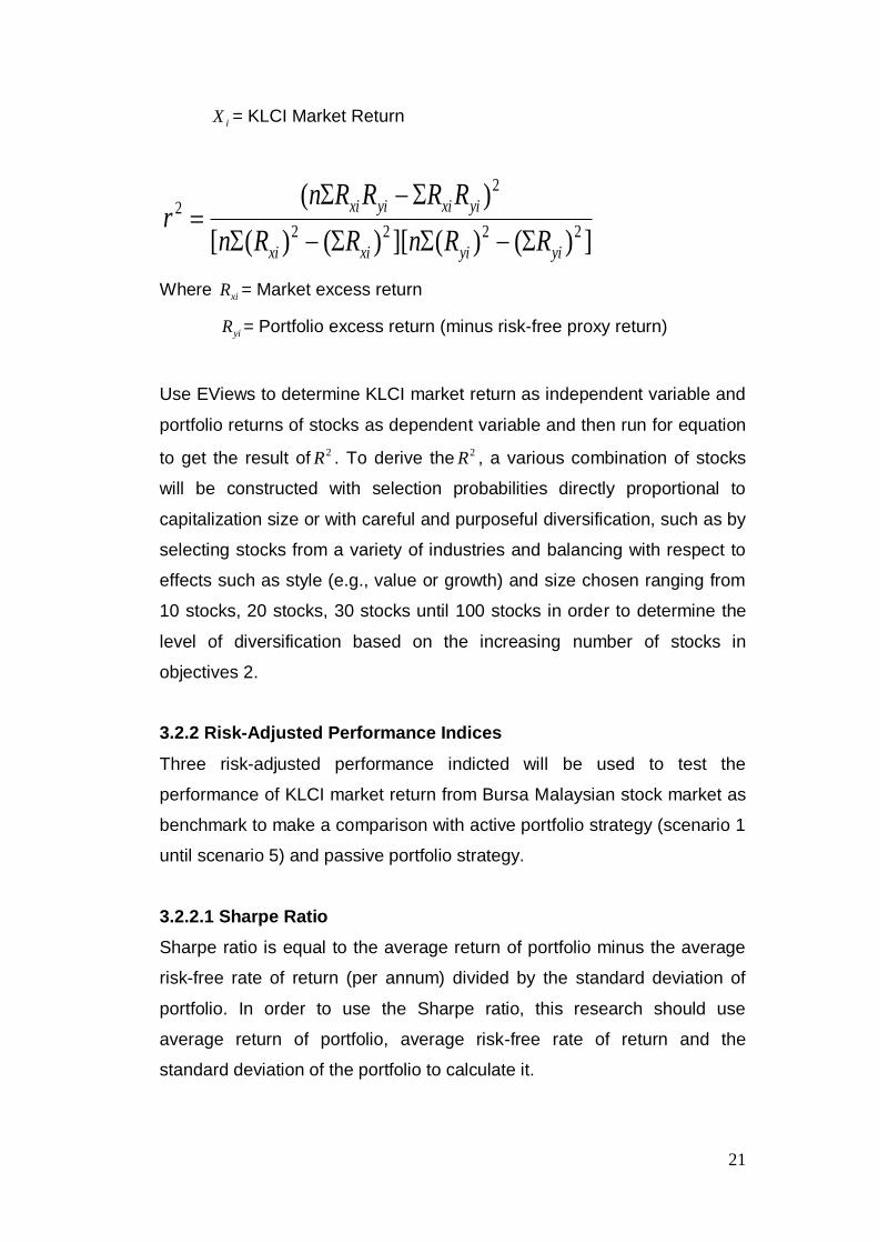
21

iX = KLCI Market Return

])()(][)()([

)(2222

2

2

yiyixixi

yixiyixi

RRnRRn

RRRRnr

Where xiR = Market excess return

yiR = Portfolio excess return (minus risk-free proxy return)

Use EViews to determine KLCI market return as independent variable and

portfolio returns of stocks as dependent variable and then run for equation

to get the result of 2R . To derive the 2R , a various combination of stocks

will be constructed with selection probabilities directly proportional to

capitalization size or with careful and purposeful diversification, such as by

selecting stocks from a variety of industries and balancing with respect to

effects such as style (e.g., value or growth) and size chosen ranging from

10 stocks, 20 stocks, 30 stocks until 100 stocks in order to determine the

level of diversification based on the increasing number of stocks in

objectives 2.

3.2.2 Risk-Adjusted Performance Indices

Three risk-adjusted performance indicted will be used to test the

performance of KLCI market return from Bursa Malaysian stock market as

benchmark to make a comparison with active portfolio strategy (scenario 1

until scenario 5) and passive portfolio strategy.

3.2.2.1 Sharpe Ratio

Sharpe ratio is equal to the average return of portfolio minus the average

risk-free rate of return (per annum) divided by the standard deviation of

portfolio. In order to use the Sharpe ratio, this research should use

average return of portfolio, average risk-free rate of return and the

standard deviation of the portfolio to calculate it.

22

The Sharpe ratio is presented as:

p

fp

p

rrS

Where pr = Average return of the portfolio

fr = Average risk-free rate of return (Interbank deposit rates

at the Interbank Money Market in Kuala Lumpur)

p = Standard deviation of the portfolio

The Sharpe ratio tells us whether a portfolio’s return is due to smart

investment decision or taking excess risk. If a portfolio’s Sharpe ratio is

higher, it means that a portfolio has better on its risk-adjusted performance.

The higher rate of Sharpe ratio indicates a better performance because of

each unit of total risk (standard deviation of portfolio) is rewarded with

greater excess return.

Result of average return of the portfolio and standard deviation of the

portfolio will be achieved using EViews, whereas the average risk-free rate

of return will be calculated by using Microsoft Excel. This research have

two different average risk-free rate of return which is long run from year

1998 to year 2010 and crisis period from 1st July 2007 to 30th September

2009. Since the result of average return and standard deviation of the

portfolio are provided on daily basis, therefore this research needs to

annualize average return of the portfolio by multiple 365 days and

annualize standard deviation of the portfolio by multiple 365 which is

19.1050.

3.2.2.2 Treynor Ratio

Treynor ratio is a risk-adjusted measure the return based on systematic

risk. It is quite similar with Sharpe ratio but different in which Treynor ratio

is using beta as the measurement of volatility while Sharpe ratio is using

standard deviation as the measurement of volatility. Treynor ratio is equal

to the expected return of portfolio minus the risk-free rate of return (12-

month), divided by the portfolio beta.

23

The Treynor ratio is presented as:

p

fp

p

rrT

Where

pr = Average return of the portfolio

fr = Average risk-free rate of return (Interbank deposit rates

at the Interbank Money Market in Kuala Lumpur)

p = portfolio beta

The Treynor ratio is useful for assessing the excess return, evaluating

investors to evaluate how the structure of the portfolio to different levels of

systematic risk will affect the return. However, it is only useful when a

portfolio under consideration is a sub-portfolio of a broader, fully diversified

portfolio. The higher the Treynor ratio, tells us that the better the

performance of the portfolio under analysis.

By using EViews to obtain the result of average return of the portfolio

whereas the average risk-free rate of return and portfolio beta will be

calculate by using Microsoft Excel. There will be two different average risk-

free rate of return which is long run from year 1998 to year 2010 and

another one is crisis period from 1st July 2007 to 30th September 2009.

On the other hand, market index will be used as benchmark for market

beta, and then calculates the beta using the SLOPE function on Excel.

The slope function = SLOPE (range of % change of equity, range of %

change of index). Since the result of average return of portfolio is provided

on daily basis, therefore this research needs to annualize average return

of the portfolio by multiple 365 days.

3.2.2.3 Jensen’s Index

In year 1968, Michael Jensen developed an index called Jensen’s index

also known as Jensen’s alpha. It is predicted by the CAPM, given the

portfolio’s beta and the expected market return. Jensen’s index measures

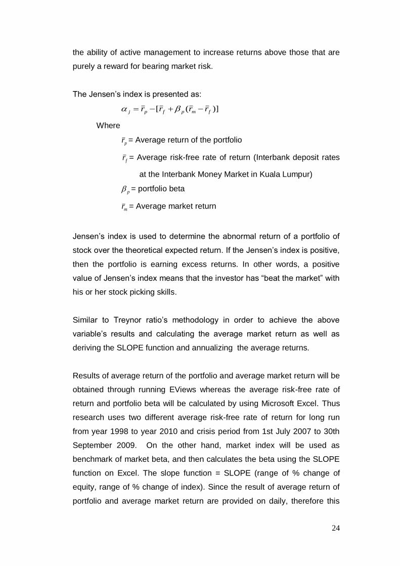
24

the ability of active management to increase returns above those that are

purely a reward for bearing market risk.

The Jensen’s index is presented as:

)]([ fmpfpj rrrr

Where

pr = Average return of the portfolio

fr = Average risk-free rate of return (Interbank deposit rates

at the Interbank Money Market in Kuala Lumpur)

p = portfolio beta

mr = Average market return

Jensen’s index is used to determine the abnormal return of a portfolio of

stock over the theoretical expected return. If the Jensen’s index is positive,

then the portfolio is earning excess returns. In other words, a positive

value of Jensen’s index means that the investor has ―beat the market‖ with

his or her stock picking skills.

Similar to Treynor ratio’s methodology in order to achieve the above

variable’s results and calculating the average market return as well as

deriving the SLOPE function and annualizing the average returns.

Results of average return of the portfolio and average market return will be

obtained through running EViews whereas the average risk-free rate of

return and portfolio beta will be calculated by using Microsoft Excel. Thus

research uses two different average risk-free rate of return for long run

from year 1998 to year 2010 and crisis period from 1st July 2007 to 30th

September 2009. On the other hand, market index will be used as

benchmark of market beta, and then calculates the beta using the SLOPE

function on Excel. The slope function = SLOPE (range of % change of

equity, range of % change of index). Since the result of average return of

portfolio and average market return are provided on daily, therefore this

25

research need to annualize average return of the portfolio by multiple 365

days.

3.2.3 Generalized Autoregressive Conditional Heteroscedasticity

model (GARCH)

Good investment should generate return in a form of low risk. Hence,

investor is trying to find the method which can measure and forecast the

volatilities of the portfolio over its holding period in order to develop best

strategy to reduce the risk and maximize return. To achieve this, this

research uses EViews to estimate the Generalized Autoregressive

Conditional Heteroscedasticity model (GARCH) to measure the portfolio

volatilities and forecasting. GARCH model is a modified formula from

ARCH model. As mentioned earlier, this research has narrowed the

strategy to active portfolio strategy and passive portfolio strategy. For

active portfolio holder, they will actively trade their shares in the portfolio;

hence volatilities measure will be important. While for the passive portfolio,

they tend to hold the portfolio until the maturity, hence the volatilities

measure will not be equally important. However, as this research is

analyzing the volatility to determine which strategy is the best, and has the

lowest volatilities, so this research run test on all types of portfolios.

ARCH is a model to test whether the conditional variance are cause by its

own lagged term. The model is:

The is the time varying variance, which is a function of a constant

term ) plus a lagged once, the square of the error in the previous period

( ). For the GARCH to be significant, the ARCH model should first be

significant. Both the and must be positive to ensure a positive

variance. The coefficient must be less than 1, otherwise will continue

to increase over time, eventually exploding. Besides that, the Obs*R-

squared (LM statistic) and the F-statistics must be significant.

26

After that, this research will proceed to estimate the GARCH model. The

GARCH model is a model which combines the MA (moving average) into

ARCH model. Which its final output of coefficient indicates its volatilities

whether cause by new information (α) or its own MA (β) effect. The model

is:

As this research includes one past lag time varying variance as regressor.

The coefficient of represent the ARCH effect; it is the level of volatilities

due to the new information. While the coefficient represent the MA effect,

which indicates the volatilities that caused by its own lag moving average

effect. For the GARCH model to be valid, both of the coefficient and

must be significant and have positive value, and sum of these values must

below 1. If sum of this 2 value are above 1, it is a so-called integrated

GARCH process, or IGARCH. In the IGARCH, it appears because it

estimates with using a long time-series of stock return. It can yield a very

parsimonious representation of the distribution of an asset’s return. In

some respect, this constraint forces the conditional variance to act like a

process with a unit-root. It is useful in forecasting, where one-step-ahead

forecast of the conditional variance is:

And the j-step-ahead forecast is

Moreover, the unconditional variance is clearly infinite, the IGARCH is not

perfect. This research will use GARCH model for 4 steps process. Firstly,

test the ARCH effect of all types of portfolios, to see whether all portfolios

have the problem of ARCH. Second, if there appear to be some portfolios

do not show ARCH effect, then will estimate a GARCH variance series

graph to check whether there is some potential problem that causes the

insignificant effect appeared in step 1. Next, estimate a GARCH model.

After checked its validity, then compare their volatilities by using the

coefficient to see whether which portfolio strategy does has the lowest

volatilities, and its volatilities are mostly cause by what factor, whether new

information or its own lag effect (MA). Finally, use the estimated model to

27

forecast the future GARCH variance series. This is because the

unconditional forecast has a greater variance than the conditional forecast,

hence only forecast for the 10-days-ahead value. This research should

also take consideration in the 10-days-ahead forecast with using 13 years

period data and 10-days ahead forecast with using crisis period data.

Because as mentioned above, unconditional forecast will have greater

variance, and this research is using daily data, hence the variance will be

far greater than theory mention. However, due to the purpose of getting

accurate and discrete result for volatilities comparing between portfolios,

this research insists to use daily data in measuring and forecasting.

3.2.4 Unit Root Test

To prove the non-stationarity of the data series, this research deploys

Augmented Dickey-Fuller (ADF) (1981), non-parametric Phillips-Perron

(PP) (1988), and Kwiatkowski et al. (KPSS) (1992) testing principles. This

research proceeds the testing of non-stationarity in the presence of

intercept and trend. The combining of the three tests should give a

consistent and reliable conclusion regarding the non-stationarity of the

data.

3.2.4.1 Augmented Dickey-Fuller test (ADF)

ADF test (1981) with intercept and trend is illustrated as follows:

tit

m

i

itt YYtY

1

121

Where t is a pure white noise error term and where

),(),( 322211 tttttt YYYYYY etc. The number of lagged difference

terms to include is often determined empirically, the idea being to include

enough terms so that the error term in the above equation is serially

uncorrelated, so that can obtain an unbiased estimate of 0 , the

coefficient of lagged 1tY .

28

ADF test follows the critical values to determine the test result. ADF test

takes care of possible serial correlation in the error terms by adding the

lagged difference terms of the regressand.

The hypothesis of ADF test:

:0H The data series has a unit root (non-stationary).

:1H The data series does not have a unit root (stationary).

Rule of thumb:

Reject the null hypothesis if the ADF test statistic <– critical value or ADF

test statistic> critical value.

3.2.4.2. Non-parametric Phillips-Perron test (PP)

PP test is illustrated as follows:

N

st

stt

N

t

N

t

t lsNN 111

2 ),(21

Where is truncation lag parameter; and w(s,l) is a window that is equal to

)1/(1 s . PP test follows the critical values to determine the test result.

PP test use non-parametric statistical methods to take care of the serial

correlation in the error terms without adding the lagged difference terms.

The hypothesis of PP test:

:0H The data series has a unit root (non-stationary).

:1H The data series does not have a unit root (stationary).

Rule of thumb:

Reject the null hypothesis if the PP test statistic <– critical value or PP

test statistic> critical value.

29

3.2.4.3 Kwiatkowski et al. test (KPSS)

The null hypothesis for the KPSS test is stationary (does not have a unit

root). KPSS is a semi-parametric procedure tests for stationary against the

alternative of a unit root. It uses the LM statistic to determine the test

results.

Let , t= 1,2,3 ……, T, be the residuals from the regression of y on an

intercept and time trend. Let 2ˆ be the estimate of the error variance from

this regression (the sum of squared residuals, divided by T). Define the

partial sum process of the residuals:

i

t

it eS

1

, t= 1,2,……, T.

Then the LM (and LBI) statistic is

LM = 22

1

ˆ/ t

T

i

S

The hypothesis of KPSS test:

:0H The data series is stationary.

:1H The data series is non-stationary.

Rule of thumb:

Reject the null hypothesis if the KPSS test statistic > the LM critical value.

3.2.5 VAR Lag Order Selection Criteria

After proving the non-stationarity of the data series, the optimal lag length

used to run the cointegration test need to be selected. The criteria includes

the sequential modified LR test statistic, Final Prediction and Error, Akaike

Information Criterion, Schwarz information critierion, and Hannan-Quinn

information criterion. The common practice in financial research has been

based on the AIC. To generate a more comprehensive result, this

research will determine the optimal lag length based on both AIC and SC.

The models with the lowest AIC and SC will be chosen.

30

3.2.5.1 Akaike’s Information Criterion (AIC)

The AIC criterion is defined as:

AIC= n

RSSe

n

ue nkink /2

2/2 ˆ

Where k is the number of regressors (including the intercept) and n is the

number of the observations. For mathematical convenience, it is written as:

ln AIC=

n

RSS

n

kln

2

where ln AIC = natural log of AIC and nk /2 = penalty factor. The model

with the lowest value of AIC will be selected.

3.2.5.2 Schwarz’s Information Criterion (SIC)

The SC criterion is defined as:

SC= n

RSSn

n

un nknk /

2

/ˆ

or in log-form:

ln SC=

n

RSSn

n

klnln

where [ nnk ln)/( ] is the penalty factor. The model with the lowest value of

SC will be selected.

3.2.6 Johansen and Juselius Cointegration Test

Stock prices, which are always known to be non-stationary in nature, with

cointegration means that the price series cannot wander off in opposite

directions for very long without coming back to a mean distance eventually.

Hence, a diversified portfolio should be free from cointegration. Alexander

(1999) argued that the cointegration based portfolio is a better model than

the correlation based portfolio which was introduced by Markowitz in 1959.

The underlying reason is that correlation is intrinsically a short run

measure, and thus the figure is misleading because a high negative

correlation in a short period can constitute a low correlation to the overall

portfolio. Thus, comparison is to be made between a portfolio with lowest

31

correlation (correlation based portfolio) and a portfolio free from any

cointegration (cointegration based portfolio). Cointegration based portfolio

is constructed using the Johansen and Juselius cointegration test. After

proving the non-stationarity of the stock prices series, they can be used to

run the Johansen and Juselius cointegration test with the determined

optimal lag length.

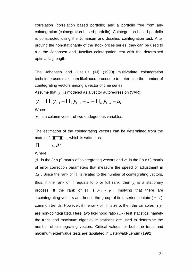
The Johansen and Juselius (JJ) (1990) multivariate cointegration

technique uses maximum likelihood procedure to determine the number of

cointegrating vectors among a vector of time series.

Assume that ty is modeled as a vector autoregression (VAR):

tktkttt yyyy ...2211

Where:

ty is a column vector of two endogenous variables.

The estimation of the cointegrating vectors can be determined from the

matrix of , which is written as:

'

Where:

' is the ( r x p) matrix of cointegrating vectors and is the ( p x r ) matrix

of error correction parameters that measure the speed of adjustment in

ty . Since the rank of is related to the number of cointegrating vectors,

thus, if the rank of equals to p or full rank, then ty is a stationary

process. If the rank of is pr 0 , implying that there are

r cointegrating vectors and hence the group of time series contain )( rp

common trends. However, if the rank of is zero, then the variables in ty

are non-cointegrated. Here, two likelihood ratio (LR) test statistics, namely

the trace and maximum eigenvalue statistics are used to determine the

number of cointegrating vectors. Critical values for both the trace and

maximum eigenvalue tests are tabulated in Osterwald-Lenum (1992)

32

The trace statistics test the )(0 rH against )(1 pH , and is written as:

Trace = )1ln(1

^

i

p

riT

On the other hand, the maximum eigenvalue statistic tests the )(0 rH

against )1(1 rH , which is given by:

Maximum eigenvalue = )-ln(1 1

^

rT

The hypothesis of the JJ test:

:0H There is no cointegration among the data series.

:1H There is at least a cointegration among the data series.

Rule of Thumb:

If the Trace statistic and Max-Eigen Statistic are larger than their 0.05

critical values respectively, the null hypothesis is rejected.

3.3 Hypotheses

1.) :0H There is no significant ARCH effect between past volatile and

current volatile.

:1H There is significant ARCH effect between past volatile and

current volatile.

2.) :0H There is no significant GARCH effect between past volatile and

current volatile.

:1H There is significant GARCH effect between past volatile and

current volatile.

3.) :0H There is no significant of cointegration among the data series.

:1H There is at least one cointegration among the data series.

33

3.4 Summary of Methodologies

Data collection is based on sample study of 100 stocks with highest

earnings in fiscal year 2009 from Bursa Malaysia with closing price

collected on daily basis with a period of 13 years from year 1998 to 2010

where all data are retrieved from Bursa Station. After that, under objective

1 the performances of active and passive strategy in long run of 13 years

period and crisis period will be examined. Under objective 2, 2R will be

used to determine the level of diversification of the portfolios where in

objective 3 diversification level achieved by correlation based and co-

integration based portfolio in the crisis period and long run will be

compared.

Model designs involved in examining objective 1 are descriptive statistics

which are arithmetic mean and standard deviation to calculate portfolio

return where in risk-adjusted indices 3 ratios which are Sharpe ratio,

Treynor ratio and Jensen Index will be used to determine which portfolio

gives the highest performance in long run as well as during crisis period

and next Generalized Autoregressive Conditionally Heteroskedastic

(GARCH) is run to measure the volatilities between the active and passive

portfolios. For GARCH model, it involves 4 steps of process. The first step

is to estimate the ARCH model, which is the requirement of GARCH model.

Before estimating the GARCH model, ARCH model should prove to be

significant. Then, the second step is to estimate the GARCH variance

graph, where the purpose is to detect the outliers or potential issue that

cause the model to be insignificant. The next step is the GARCH model

estimation, which the coefficients value will be taken into comparison of

volatilities between portfolios. Finally, the last step is GARCH forecasting,

which aims to test the ability of the model in forecasting.

2R will be used to determine the level of diversification of portfolio under

objective 2 while in objective 3 correlation based and cointegration based

portfolio in the crisis period and long run will be constructed to compare

the level of diversification achieved. In the process of constructing

34

cointegration based portfolio, trial and error is conducted. A portfolio of 15

stocks is randomly selected in the sample. First, unit root tests including

Augmented Dickey-Fuller test (ADF), Non-parametric Phillips-Perron test

(PP), Kwiatkowski et al. test (KPSS) will be used to prove the stock price

series within the constructed portfolio is non-stationary. After that, the

optimal lag length to run Johansen and Juselius Cointegration Test is

determined through VAR Lag Order Selection Criteria based on Akaike’s

Information Criterion (AIC) and Schwarz’s Information Criterion (SC).

Finally, Johansen and Juselius Cointegration Test is conducted to

determine if there is any cointegration within the portfolio. The portfolio

without any cointegration among the stock price movement will be

selected as the cointegration based portfolio in this research.

35

CHAPTER 4.0 DATA RESULTS

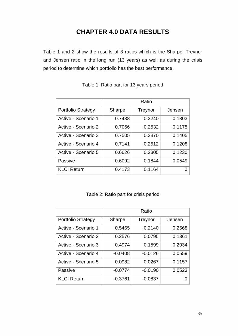
Table 1 and 2 show the results of 3 ratios which is the Sharpe, Treynor

and Jensen ratio in the long run (13 years) as well as during the crisis

period to determine which portfolio has the best performance.

Table 1: Ratio part for 13 years period

Ratio

Portfolio Strategy Sharpe Treynor Jensen

Active - Scenario 1 0.7438 0.3240 0.1803

Active - Scenario 2 0.7066 0.2532 0.1175

Active - Scenario 3 0.7505 0.2870 0.1405

Active - Scenario 4 0.7141 0.2512 0.1208

Active - Scenario 5 0.6626 0.2305 0.1230

Passive 0.6092 0.1844 0.0549

KLCI Return 0.4173 0.1164 0

Table 2: Ratio part for crisis period

Ratio

Portfolio Strategy Sharpe Treynor Jensen

Active - Scenario 1 0.5465 0.2140 0.2568

Active - Scenario 2 0.2576 0.0795 0.1361

Active - Scenario 3 0.4974 0.1599 0.2034

Active - Scenario 4 -0.0408 -0.0126 0.0559

Active - Scenario 5 0.0982 0.0267 0.1157

Passive -0.0774 -0.0190 0.0523

KLCI Return -0.3761 -0.0837 0

36

Table 3 and 4 show the ARCH outputs which include: coefficients, F-

statistic, Probabilities for F-statistic, obs*R-squared, and probabilities for

obs*R-squared. The primary usage for these outputs is to check the

validity of models.

Table 3: ARCH coefficients, F-statistics and Obs*R-squared for 13 years

period

13 years

period

(Portfolio

Strategy) α0 α1 F-statistic Prob.

Obs*R-

squared Prob.

Active –

scenario

1 0.000338 0.13846 62.585350 0.000000 61.423870 0.000000

Active –

scenario

2 0.000134 0.48281 973.276500 0.000000 746.867400 0.000000

Active –

scenario

3 0.000169 0.37814 534.229200 0.000000 458.127800 0.000000

Active –

scenario

4 0.000103 0.62064 2006.218000 0.000000 1234.188000 0.000000

Active –

scenario

5 0.000187 0.51508 1156.312000 0.000000 850.059500 0.000000

Passive 0.000084 0.48230 970.936500 0.000000 745.489500 0.000000

KLCI

Return 0.000106 0.50119 1074.575000 0.000000 805.069200 0.000000

37

Table 4: ARCH coefficients, F-statistics and Obs*R-squared for crisis

period

Crisis

time

(Portfolio

Strategy) α0 α1 F-statistic Prob.

Obs*R-

squared Prob.

Active –

scenario

1 0.000268 0.14251 11.504080 0.000744 11.311080 0.000770

Active –

scenario

2 0.000144 0.20846 25.215950 0.000001 24.206990 0.000001

Active –

scenario

3 0.000186 0.05913 1.946986 0.163470 1.947171 0.162892

Active –

scenario

4 0.000124 0.22855 30.585180 0.000000 29.092180 0.000000

Active –

scenario

5 0.000198 0.11260 7.125424 0.007822 7.060455 0.007880

Passive 0.000094 0.11715 7.722201 0.005639 7.643675 0.005697

KLCI

Return 0.000125 0.07875 3.462697 0.063296 3.453628 0.063113

38

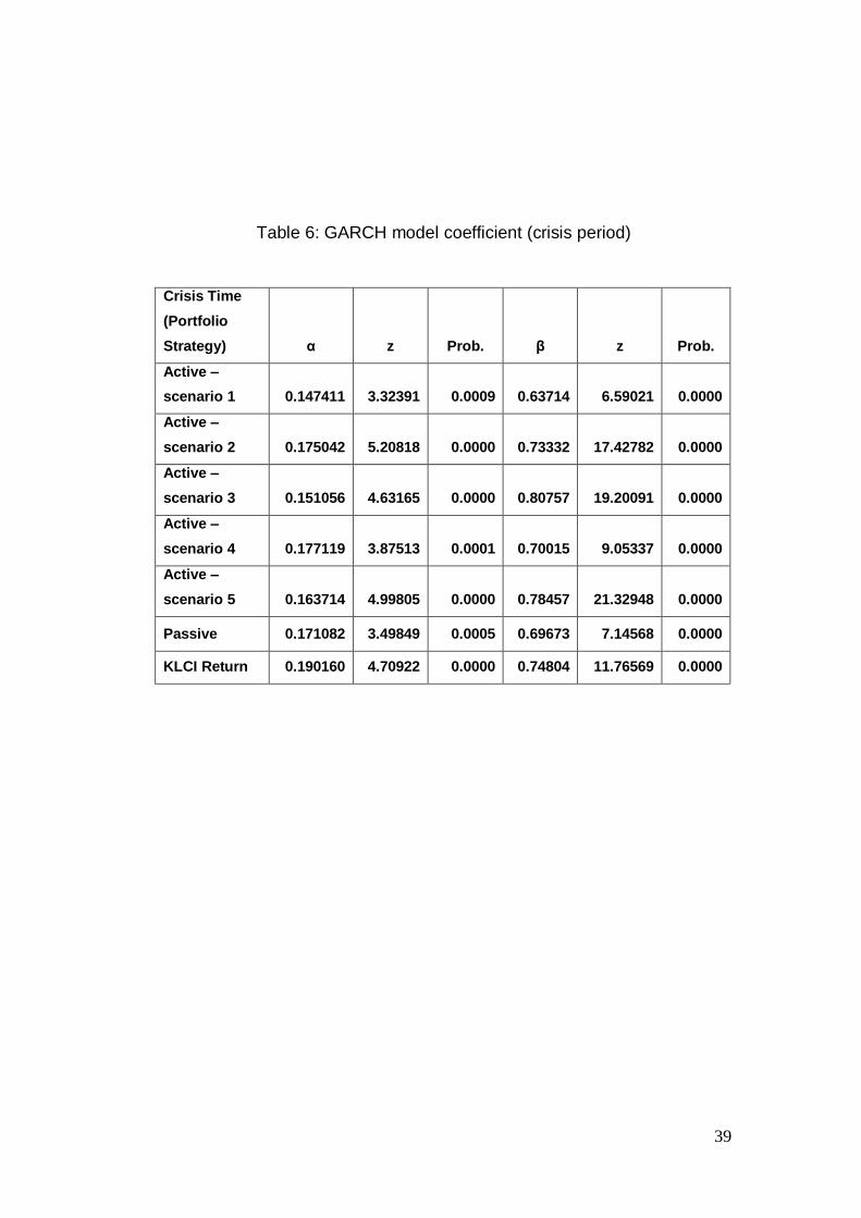
Table 5 and 6 show the estimated GARCH outputs which included the

coefficient value, z-Statistic, and probabilities for the coefficient. The

values of coefficients represent the volatilities due to new market

information and its own MA effect, while the z-statistic and probabilities

represent the significant level of model.

Table 5: GARCH model coefficient (13 years period)

13 years period

data

(Portfolio

Strategy) α z Prob. β z Prob.

Active –

scenario 1 0.215164 20.33276 0.0000 0.787730 70.60464 0.0000

Active –

scenario 2 0.159353 21.26537 0.0000 0.831008 139.93440 0.0000

Active –

scenario 3 0.219385 26.36326 0.0000 0.752648 72.81332 0.0000

Active –

scenario 4 0.130107 19.08184 0.0000 0.856565 133.09350 0.0000

Active –

scenario 5 0.138294 16.60279 0.0000 0.858470 124.28470 0.0000

Passive 0.141177 18.28669 0.0000 0.850164 121.33330 0.0000

KLCI Return 0.138588 18.48601 0.0000 0.866065 140.18460 0.0000

39

Table 6: GARCH model coefficient (crisis period)

Crisis Time

(Portfolio

Strategy) α z Prob. β z Prob.

Active –

scenario 1 0.147411 3.32391 0.0009 0.63714 6.59021 0.0000

Active –

scenario 2 0.175042 5.20818 0.0000 0.73332 17.42782 0.0000

Active –

scenario 3 0.151056 4.63165 0.0000 0.80757 19.20091 0.0000

Active –

scenario 4 0.177119 3.87513 0.0001 0.70015 9.05337 0.0000

Active –

scenario 5 0.163714 4.99805 0.0000 0.78457 21.32948 0.0000

Passive 0.171082 3.49849 0.0005 0.69673 7.14568 0.0000

KLCI Return 0.190160 4.70922 0.0000 0.74804 11.76569 0.0000

40

Figure 1 and 2 are the estimated GARCH variance series graphs. They

are used to detect the outliers and potential problem that cause the model

to be insignificant.

Figure 1: GARCH graph for all types of portfolio (13 years period)

41

Figure 2: GARCH graph for all types of portfolio (crisis period)

42

Table 7 and 8 show the forecasted GARCH value and the real GARCH

value. The last column is the differences of forecasted value from the real

value which the equation is (real value – forecasted value) / real value.

Table 7: GARCH forecasting (by using 13 years period data)

Active

scenario 1

Active

scenario 2

Forecasted Real

Difference

from real

Forecasted Real

Difference

from real

0.0003000 0.0003000 0.0000%

0.0001450 0.0001450 0.0000%

0.0003650 0.0006300 42.0635%

0.0002130 0.0001980 -7.5758%

0.0003840 0.0003640 -5.4945%

0.0002520 0.0002200 -14.5455%

0.0003900 0.0003040 -28.2895%

0.0002760 0.0001410 -95.7447%

0.0003920 0.0003410 -14.9560%

0.0002890 0.0001270 -127.5591%

0.0003920 0.0002750 -42.5455%

0.0002980 0.0001710 -74.2690%

0.0003930 0.0002890 -35.9862%

0.0003020 0.0001560 -93.5897%

0.0003930 0.0003970 1.0076%

0.0003050 0.0001350 -125.9259%

0.0003930 0.0002750 -42.9091%

0.0003070 0.0001530 -100.6536%

0.0003930 0.0003400 -15.5882%

0.0003080 0.0001330 -131.5789%

Mean -14.2698%

Mean -77.1442%

Active

scenario 3

Active

scenario 4

Forecasted Real

Difference

from real

Forecasted Real

Difference

from real

0.0001610 0.0001610 0.0000%

0.0001560 0.0001560 0.0000%

0.0002320 0.0001950 -18.9744%

0.0002130 0.0001650 -29.0909%

0.0002680 0.0003730 28.1501%

0.0002390 0.0002420 1.2397%

0.0002860 0.0001510 -89.4040%

0.0002500 0.0001660 -50.6024%

0.0002950 0.0001730 -70.5202%

0.0002560 0.0002150 -19.0698%

0.0003000 0.0001500 -100.0000%

0.0002580 0.0001430 -80.4196%

0.0003020 0.0001500 -101.3333%

0.0002590 0.0001480 -75.0000%

0.0003030 0.0001930 -56.9948%

0.0002600 0.0001420 -83.0986%

0.0003040 0.0001500 -102.6667%

0.0002600 0.0001550 -67.7419%

0.0003040 0.0003880 21.6495%

0.0002600 0.0002200 -18.1818%

Mean -49.0094%

Mean -42.1965%

43

Table 7: GARCH forecasting (by using 13 years period data)

Active

scenario 5

Passive

portfolio

Forecasted Real

Difference

from real

Forecasted Real

Difference

from real

0.0002000 0.0001990 -0.5025%

0.0000781 0.0000788 0.8883%

0.0003140 0.0003080 -1.9481%

0.0001210 0.0008020 84.9127%

0.0003830 0.0002160 -77.3148%

0.0001440 0.0000810 -77.7778%

0.0004240 0.0001940 -118.5567%

0.0001560 0.0000976 -59.8361%

0.0004480 0.0002070 -116.4251%

0.0001630 0.0000862 -89.0951%

0.0004630 0.0001940 -138.6598%

0.0001670 0.0000862 -93.7355%

0.0004710 0.0001940 -142.7835%

0.0001690 0.0000922 -83.2972%

0.0004770 0.0001970 -142.1320%

0.0001700 0.0000943 -80.2757%

0.0004800 0.0002110 -127.4882%

0.0001710 0.0000787 -117.2808%

0.0004820 0.0002680 -79.8507%

0.0001710 0.0000835 -104.7904%

Mean -94.5661%

Mean -62.0288%

KLCI

Return

Forecasted Real

Difference

from real

0.0000935 0.0000935 0.0000%

0.0001510 0.0000935 -61.4973%

0.0001930 0.0001420 -35.9155%

0.0002250 0.0001800 -25.0000%

0.0002480 0.0001380 -79.7101%

0.0002650 0.0000819 -223.5653%

0.0002780 0.0000842 -230.1663%

0.0002880 0.0001080 -166.6667%

0.0002950 0.0000818 -260.6357%

0.0003000 0.0000837 -258.4229%

Mean -134.1580%

44

Table 8: GARCH forecasting (by using crisis period data)

Active

scenario 1

Active

scenario 2

Forecasted Real

Difference

from real

Forecasted Real

Difference

from real

0.0002700 0.0002720 0.7353%

0.0001780 0.0001770 -0.5650%

0.0003060 0.0002730 -12.0879%

0.0001850 0.0001470 -25.8503%

0.0003110 0.0002720 -14.3382%

0.0001870 0.0001360 -37.5000%

0.0003120 0.0002740 -13.8686%

0.0001870 0.0001370 -36.4964%

0.0003120 0.0002930 -6.4846%

0.0001880 0.0001390 -35.2518%

0.0003120 0.0005080 38.5827%

0.0001880 0.0002180 13.7615%

0.0003120 0.0002720 -14.7059%

0.0001880 0.0001450 -29.6552%

0.0003120 0.0002820 -10.6383%

0.0001880 0.0001470 -27.8912%

0.0003120 0.0002840 -9.8592%

0.0001880 0.0001320 -42.4242%

0.0003120 0.0004150 24.8193%

0.0001880 0.0001360 -38.2353%

Mean -1.7845%

Mean -26.0108%

Active

scenario 3

Active

scenario 4

Forecaste

d Real

Difference

from real

Forecaste

d Real

Difference

from real

0.0001810 0.0001770 -2.2599%

0.0001320 0.0001300 -1.5385%

0.0001960 0.0001780 -10.1124%

0.0001540 0.0001300 -18.4615%

0.0001980 0.0001840 -7.6087%

0.0001580 0.0001470 -7.4830%

0.0001980 0.0001870 -5.8824%

0.0001580 0.0001290 -22.4806%

0.0001980 0.0001820 -8.7912%

0.0001580 0.0001310 -20.6107%

0.0001980 0.0001800 -10.0000%

0.0001580 0.0001420 -11.2676%

0.0001980 0.0001790 -10.6145%

0.0001580 0.0001290 -22.4806%

0.0001980 0.0001780 -11.2360%

0.0001580 0.0001290 -22.4806%

0.0001980 0.0001780 -11.2360%

0.0001580 0.0001290 -22.4806%

0.0001980 0.0001810 -9.3923%

0.0001580 0.0001300 -21.5385%

Mean -8.7133%

Mean -17.0822%

45

Table 8: GARCH forecasting (by using crisis period data)

Active

scenario 5

Passive

portfolio

Forecasted Real

Difference

from real

Forecasted Real

Difference

from real

0.0001950 0.0001920 -1.5625%

0.0001010 0.0001010 0.0000%

0.0002200 0.0001950 -12.8205%

0.0001060 0.0000999 -6.1061%

0.0002240 0.0001930 -16.0622%

0.0001060 0.0000984 -7.7236%

0.0002240 0.0001920 -16.6667%

0.0001070 0.0001590 32.7044%

0.0002240 0.0001920 -16.6667%

0.0001070 0.0001180 9.3220%

0.0002240 0.0002010 -11.4428%

0.0001070 0.0001010 -5.9406%

0.0002240 0.0001960 -14.2857%

0.0001070 0.0000975 -9.7436%

0.0002240 0.0001900 -17.8947%

0.0001070 0.0000974 -9.8563%

0.0002240 0.0001900 -17.8947%

0.0001070 0.0000978 -9.4070%

0.0002240 0.0001920 -16.6667%

0.0001070 0.0000975 -9.7436%

Mean -14.1963%

Mean -1.6494%

KLCI

Return

Forecasted Real

Difference

from real

0.0001260 0.0001240 -1.6129%

0.0001350 0.0001240 -8.8710%

0.0001350 0.0001220 -10.6557%

0.0001350 0.0001230 -9.7561%

0.0001350 0.0001220 -10.6557%

0.0001350 0.0001240 -8.8710%

0.0001350 0.0001300 -3.8462%

0.0001350 0.0001230 -9.7561%

0.0001350 0.0001220 -10.6557%

0.0001350 0.0001220 -10.6557%

Mean -8.5336%

46

Table 9 shows the R-squared results for a portfolio of randomly selected

stocks in order to determine the level of diversification.

Table 9: R-squared for each number of stocks

Portfolio

Strategy

Number of Stocks

10 20 30 40 50

R-squared 57.98% 62.46% 63.01% 66.57% 66.61%

Portfolio

Strategy

Number of Stocks

60 70 80 90 100

R-squared 67.80% 68.97% 69.17% 69.48% 70.22%

47

The stationary test results on the 15 stocks by using ADF, PP and KPSS

tests are shown in Table 10. Both the ADF and PP tests have the null

hypothesis of data series is non-stationary. KPSS has the null hypothesis

of data series is stationary. Table 11 indicates the critical values to

determine the significance of the tests. ADF and PP follow critical value,

while KPSS follows LM- Stat critical value.

Table 10: Stationary Tests on the 15 Stocks within the Cointegration

based Portfolio at level

Stocks ADF PP KPSS

aji intercept and trend -2.047854 -2.030020 0.685535***

bjtoto intercept and trend -3.405105* -3.387044* 0.581280***

carlsbg intercept and trend -2.745142 -2.294255 0.224102***

ccb intercept and trend -2.194660 -2.169843 0.692892***

gnealy intercept and trend -2.514211 -2.434966 1.112411***

kianjoo intercept and trend -2.553575 -2.606018 0.566848***

kulim intercept and trend -1.185755 -1.065605 0.912681***

maa intercept and trend -2.898170 -2.858241 0.700019***

mflour intercept and trend -1.127680 -1.069357 0.940947***

mrcb intercept and trend -2.664280 -2.615572 0.570300***

pbbank intercept and trend -2.147640 -2.431017 0.485827***

rview intercept and trend -3.070753 -3.048372 0.367537***

shchan intercept and trend -3.323005* -3.131620* 0.683991***

sime intercept and trend -2.842467 -2.645653 0.193438**

umcca intercept and trend -0.913605 -1.000442 1.229854***

*(**)[***] denotes rejection of the hypothesis at 10%(5%)[1%] significance

level.

Table 11: critical values for the unit root tests

PP ADF KPSS

Critical value LM-Stat critical value

1% significant level -3.960904 0.216000

5% significant level -3.411208 0.146000

10% significant level -3.127437 0.119000

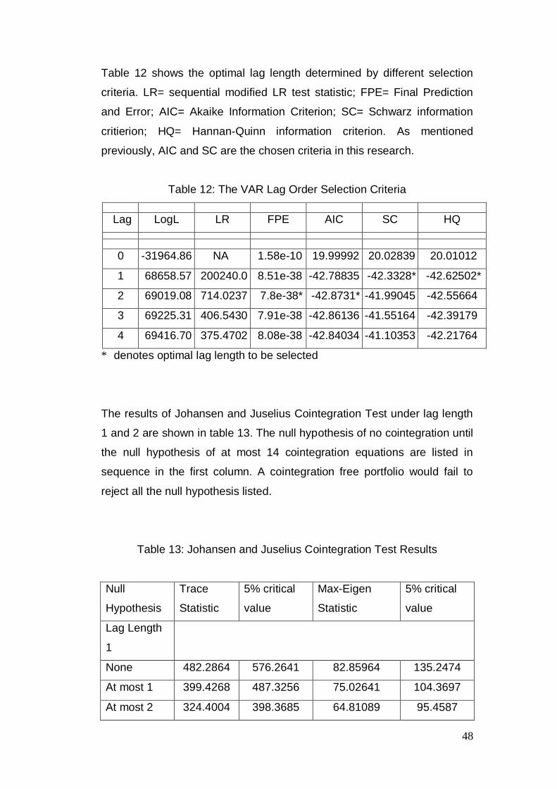
48

Table 12 shows the optimal lag length determined by different selection

criteria. LR= sequential modified LR test statistic; FPE= Final Prediction

and Error; AIC= Akaike Information Criterion; SC= Schwarz information

critierion; HQ= Hannan-Quinn information criterion. As mentioned

previously, AIC and SC are the chosen criteria in this research.

Table 12: The VAR Lag Order Selection Criteria

Lag LogL LR FPE AIC SC HQ

0 -31964.86 NA 1.58e-10 19.99992 20.02839 20.01012

1 68658.57 200240.0 8.51e-38 -42.78835 -42.3328* -42.62502*

2 69019.08 714.0237 7.8e-38* -42.8731* -41.99045 -42.55664

3 69225.31 406.5430 7.91e-38 -42.86136 -41.55164 -42.39179

4 69416.70 375.4702 8.08e-38 -42.84034 -41.10353 -42.21764

* denotes optimal lag length to be selected

The results of Johansen and Juselius Cointegration Test under lag length

1 and 2 are shown in table 13. The null hypothesis of no cointegration until

the null hypothesis of at most 14 cointegration equations are listed in

sequence in the first column. A cointegration free portfolio would fail to

reject all the null hypothesis listed.

Table 13: Johansen and Juselius Cointegration Test Results

Null

Hypothesis

Trace

Statistic

5% critical

value

Max-Eigen

Statistic

5% critical

value

Lag Length

1

None 482.2864 576.2641 82.85964 135.2474

At most 1 399.4268 487.3256 75.02641 104.3697

At most 2 324.4004 398.3685 64.81089 95.4587

49

At most 3 259.5895 354.9837 49.54621 76.57843

At most 4 210.0433 285.1425 43.49564 70.53513

At most 5 166.5477 239.2354 35.52198 64.50472

At most 6 131.0257 197.3709 29.67099 58.43354

At most 7 101.3547 159.5297 24.69739 52.36261

At most 8 76.6573 125.6154 23.02192 46.23142

At most 9 53.63538 95.75366 17.30877 40.07757

At most 10 36.32661 69.81889 12.85114 33.87687

At most 11 23.47547 47.85613 11.61074 27.58434

At most 12 11.86473 29.79707 6.444337 21.13162

At most 13 5.420012 15.49471 5.381259 14.2646

At most 14 0.039133 3.841466 0.039133 3.841466

Lag length 2

None 460.0644 574.8402 77.47156 119.0432

At most 1 382.5928 487.2101 70.75548 114.3355

At most 2 311.8373 402.3562 56.86237 89.9541

At most 3 254.975 334.9837 47.56265 76.57843

At most 4 207.4123 285.1425 40.86393 70.53513

At most 5 166.5484 239.2354 34.96367 64.50472

At most 6 131.5847 197.3709 28.46169 58.43354

At most 7 103.123 159.5297 25.38422 52.36261

At most 8 77.73879 125.6154 23.05454 46.23142

At most 9 54.68425 95.75366 18.96617 40.07757

At most 10 35.71809 69.81889 12.92945 33.87687

At most 11 22.78864 47.85613 11.56369 27.58434

At most 12 11.22495 29.79707 6.161161 21.13162

At most 13 5.063786 15.49471 5.063428 14.2646

At most 14 0.000358 3.841466 0.000358 3.841466

* denotes rejection of the hypothesis at 5% significance level.

Comparison between correlation and cointegration based portfolio is

shown in Table 14. R-squared is used as the measure to assess the level

50

0

10

20

30

40

50

60

500 1000 1500 2000 2500 3000

SHCHAN

SHELL

MUDA

MISC

TALAM

DLADY

PMHLDG

UAC

IRCB

BAT

MUIPROP

YTLLAND

NESTLE

MUIIND

TIME

of diversification achieved by both portfolios. The higher R-squared proves

the higher level of diversification, and vice versa.

Table 14: R-squared for Correlation and Cointegration based portfolio

The stock prices movement within each portfolio in the long run and crisis

period is illustrated in Figure 3 to Figure 6.

Figure 3: The Stock Prices Movement within the Correlation based

Portfolio in the long run

Long Run Crisis Period

Correlation

based

protfolio

Cointegration

based portfolio

Correlation

based

protfolio

Cointegration

based portfolio

R-

squared 41.05% 67.16% 32.28% 55.92%

51

0

2

4

6

8

10

12

14

16

500 1000 1500 2000 2500 3000

AJIBJTOTOCARLSBGCCBGNEALY

KIANJOOKULIMMAAMFLOURMRCB

PBBANKRVIEWSHCHANSIMEUMCCA

0

10

20

30

40

50

100 200 300 400 500 600

SHCHANSHELLMUDAMISCTALAM

DLADYPMHLDGUACIRCBBAT

MUIPROPYTLLANDNESTLEMUIINDTIME

Figure 4: The Stock Prices Movement within the Cointegration based

Portfolio in the long run.

Figure 5: The Stock Prices Movement within the Correlation based

Portfolio in the crisis period.

52

0

2

4

6

8

10

12

14

100 200 300 400 500 600

AJIBJTOTOCARLSBGCCBGNEALY

KIANJOOKULIMMAAMFLOURMRCB

PBBANKRVIEWSHCHANSIMEUMCCA

Figure 6: The Stock Prices Movement within the Cointegration based

Portfolio in the crisis period.

53

CHAPTER 5.0 INTERPRETATION OF RESULTS

5.1 Risk-Adjusted Performance Indices (Sharpe, Treynor

and Jensen’s index)

Table 1 and Table 2 showed the three main ratios which is Sharpe,

Treynor and Jensen measures in order to determine the performance of

both active and passive portfolios against each other as well as the KLCI

market return in 5 different scenarios in the long run period of 13 years

and a specific period during the crisis.

In the long run, results in Table 1 showed that active and passive portfolio

in all five scenarios consistently outperforming the market return bringing

significant positive values in both Sharpe and Treynor ratios. Results

indicated that active portfolio in all five scenarios in all 3 of the measures

have higher ratios than passive portfolio which means that in long run

active portfolio management spurred out higher performance than passive

strategies. In terms of choosing the best portfolio, portfolio with the highest

performance measure would be chosen as the best portfolio performance.

To determine which strategy perform better, the higher the ratio is, the

better the performance of the portfolio.

Overall, active portfolio scenario 1 has given the highest performance over

the rest of the scenario at a diversification of 15 stocks. Based on Table 1,

both active and passive portfolio outperformed the market return which is

0.4173 in Sharpe ratio and a Treynor ratio of 0.1164. However, active

portfolio showed higher Sharpe ratio which is 0.7438 compared to passive

portfolio of 0.6092. For Treynor measure, both portfolios outperformed the

KLCI market return ratio of 0.1164 similar to Sharpe ratio. However, active

portfolio once again showed the higher Treynor ratio which is 0.3240

compared to passive portfolio with ratio of 0.1844. For Jensen ratio, the

higher the ratio, the better the risk-adjusted return resulted in a positive

Alpha value. From Table 1, both portfolios showed positive ratios which

reflect that the portfolios performance are relatively superior compared to

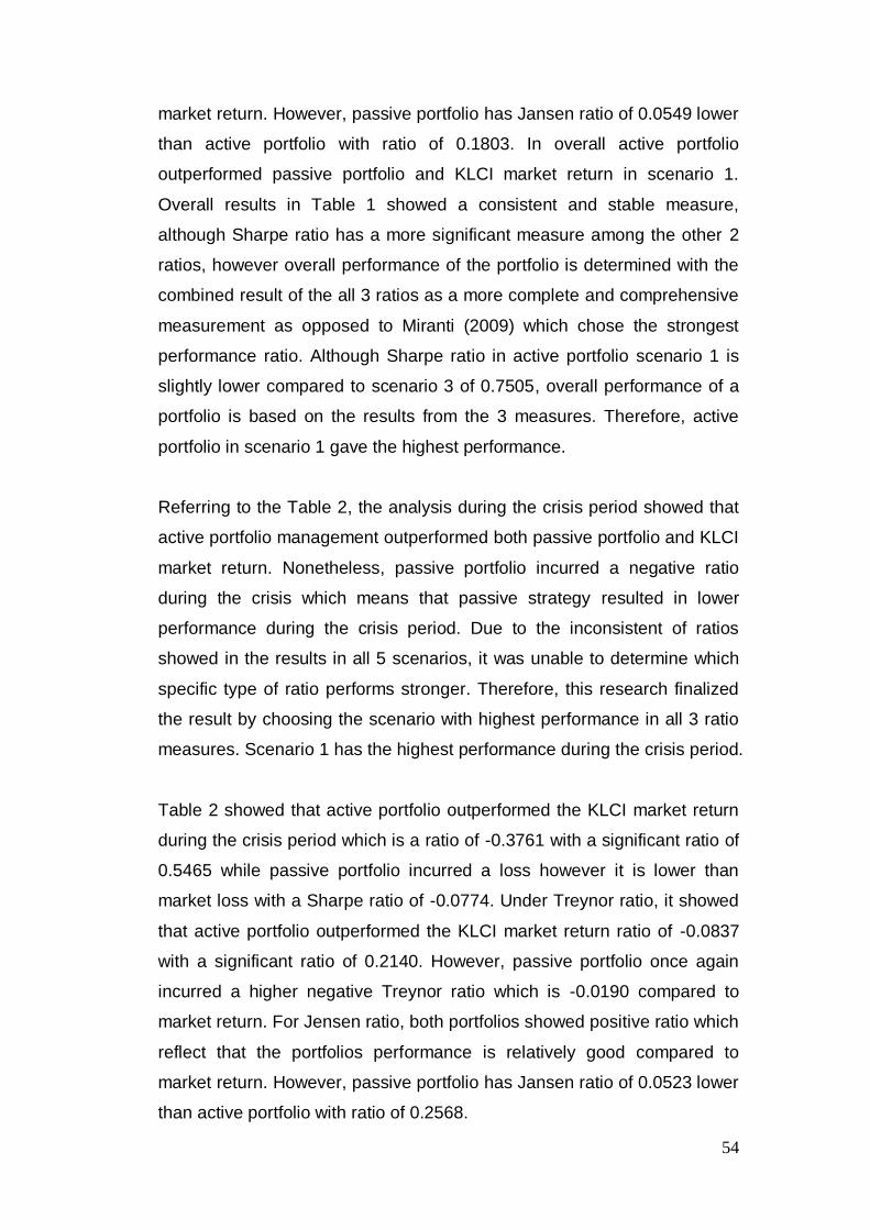
54

market return. However, passive portfolio has Jansen ratio of 0.0549 lower

than active portfolio with ratio of 0.1803. In overall active portfolio

outperformed passive portfolio and KLCI market return in scenario 1.

Overall results in Table 1 showed a consistent and stable measure,

although Sharpe ratio has a more significant measure among the other 2

ratios, however overall performance of the portfolio is determined with the

combined result of the all 3 ratios as a more complete and comprehensive

measurement as opposed to Miranti (2009) which chose the strongest

performance ratio. Although Sharpe ratio in active portfolio scenario 1 is

slightly lower compared to scenario 3 of 0.7505, overall performance of a

portfolio is based on the results from the 3 measures. Therefore, active

portfolio in scenario 1 gave the highest performance.

Referring to the Table 2, the analysis during the crisis period showed that

active portfolio management outperformed both passive portfolio and KLCI

market return. Nonetheless, passive portfolio incurred a negative ratio

during the crisis which means that passive strategy resulted in lower

performance during the crisis period. Due to the inconsistent of ratios

showed in the results in all 5 scenarios, it was unable to determine which

specific type of ratio performs stronger. Therefore, this research finalized

the result by choosing the scenario with highest performance in all 3 ratio

measures. Scenario 1 has the highest performance during the crisis period.

Table 2 showed that active portfolio outperformed the KLCI market return

during the crisis period which is a ratio of -0.3761 with a significant ratio of

0.5465 while passive portfolio incurred a loss however it is lower than

market loss with a Sharpe ratio of -0.0774. Under Treynor ratio, it showed

that active portfolio outperformed the KLCI market return ratio of -0.0837

with a significant ratio of 0.2140. However, passive portfolio once again

incurred a higher negative Treynor ratio which is -0.0190 compared to

market return. For Jensen ratio, both portfolios showed positive ratio which

reflect that the portfolios performance is relatively good compared to

market return. However, passive portfolio has Jansen ratio of 0.0523 lower

than active portfolio with ratio of 0.2568.

55

All active portfolios have outperformed the market downturn during the

crisis however there is an exception with scenario 4 where incurred low

performance during the crisis. This could be due to active portfolio in

scenario 4 holds a large proportion of property stocks which consists of 7

property stocks out of 15 stocks in a portfolio. This is consistent with the

incident of Subprime crisis in year 2008 where during the crisis most of the

stocks which were adversely affected are property related stocks. Active

portfolio under scenario 1 consists of 5 consumer stocks which hold a

large proportion in a portfolio eventually proven to be the best performer

during crisis may imply that consumer stocks generally provide protection

against downside risk as most of the products sold are necessities.

Therefore, there is still a strong demand on consumer products throughout

the period including crisis period and it is implied that these stocks are

crisis resistant and would generate profit during market downturn. The

results showed that the performance of the portfolio could be attributed by

the industry of the related stocks.

In overall, active portfolio significantly outperformed passive portfolio and

KLCI market return in long run and crisis period. The performance of

passive strategy during the crisis period is not as good as it is in the long

run. This indicated that diversification under passive portfolio strategy does

not provide as much risk reduction in crisis period compared with long run.

5.2 GARCH Model

5.2.1 ARCH output (significance of model)

Based on the Table 3, as required by theory, both the coefficient and

must be positive, and must be less than 1. The KLCI market and all the

portfolios fulfilled this requirement. Then, all the F-statistic and 2R are

significant at level of 1%. It showed that there is ARCH effect for all the

portfolios constructed with 13 years time period. Hence, the null

hypothesis of there is no significant ARCH effect between current volatile

and past volatile has been rejected.

56

For the crisis period analysis; based on Table 4, as required by theory,

both the coefficient and must be positive, and must be less than 1.

All the portfolios fulfilled this requirement. Except for active portfolio

scenario 3 and KLCI market return, all portfolio are significant at 1% level

with the F-statistic and Obs*R-squared. It could be due to the fact that one

of the companies in portfolio, which is AMOLEK has stop its trading for

some time and thus led to no movement of price, and flattened the return

of the portfolio. Other than that, for KLCI market return is insignificant in

5% level, but significant at 10% level. In overall, all the portfolios are

significant.

5.2.2 GARCH Graph

Refer to Figure 1, the active portfolio in scenario 1 showed a high volatility

in the days around 800th. It was due to the inactive trading of stock

YTLLAND before 9th May 2001, while at 10th May 2001, it started to trade

again and the price boosted from RM0.1050 to RM0.7050. While at the

days around 500th, all portfolios showed high volatility or large increase in

prices. The exact date was 3 September 1998 and 4 September 1998,

which KLCI hit historical lowest at point 262.7 at the date 1 September

1998, and at the 2 particular days, the market rebounded. While for active

portfolio scenario 3, it also showed a high volatility in days around 1350 th.

It was also due to the inactive of stock MBFHLDG before 6th June 2003,

and the price shot up from RM0.2050 to RM 0.7250 at date 9th June 2003.

5.2.3 GARCH Output

From Table 5, all the coefficients are significant at 1% level, including with

high z-stat value, it implied that the GARCH model does fit very well with

the data. Hence, the null hypothesis of there is no significant GARCH

effect between current volatile and past volatile has been rejected. While

for the active portfolio scenario 1 and KLCI market return, the sum of the

coefficient are above 1 which are 1.002894 for active portfolio scenario 1

and 1.0046653 for KLCI market return. Therefore, they resulted an

IGARCH appearance in the analysis. This indicated that the constraint

57

forces the conditional variance to act like a process with a unit-root. Hence,

it is useful for step-ahead forecast.

For the active portfolio scenario 1, its α value is 0.215164, it is the second

highest value among all other portfolios. This indicated that the portfolio

return’s volatility caused by the new market information. While for its β

value 0.78773, it showed the second lowest value among all portfolios.

This implied that its volatilities caused by its MA effect itself are low

compare with other portfolios. The results shown seem to be contradicting

with the Harry Markowitz portfolio theory, which uses the correlation

analysis to construct portfolio. It is because active portfolio scenario 1 did

not earn the lowest conditional variance among all active portfolios under

different scenarios. It is align with the research done by Christopher, David

& Francis (2010), which indicated that using correlation as a method of

portfolio constructing does not necessary yield the best result.

In active portfolio scenario 2, its α value of 0.159353 which is far lower

than the active portfolio scenario 1. While come to the β value at 0.831008,

which is the third lowest value among all portfolio. For the active portfolio

scenario 3, its α value of 0.219385 seems to be the highest value among

all others portfolios, this indicated that its volatilities are mostly affected by

the new information among all portfolios. While come to the β value, it has

the lowest value of 0.752648. Next, the active portfolio scenario 4, its α

value of 0.130107 is the lowest value among all portfolios. While come to

the β value, it has the third highest value of 0.856565. Come to the active

portfolio scenario 5, its value of 0.138294 is the second lowest among all

other portfolios. While come to the β value, it has the second highest value

of 0.858470.

In passive portfolio, its α value of 0.141177, which is the fourth lowest

value among all other portfolios. Since the value is lower than the active

portfolio scenario 1 value, it showed that, passive portfolio reacted better

than active portfolio with regards to the new information. However, it did

not outperform all active portfolios; rather it is just better than active

58

portfolio scenario 1. While with the β value of 0.850164, the figure is on the

middle point among those of other portfolios. Comparing with the active

portfolio scenario 1, it showed poorer performance. By comparing the

value of both coefficients, it could not determine which is performing better

than the other, and the value seems to be contradicting with Harry

Markowitz modern Portfolio Theory which lowest correlation should earn a

more stable return.

Looking at the KLCI market return, its α value of 0.138588 is lower than

passive portfolio and active portfolio scenario 1, which indicated that the

market reacts better than this two portfolio with regarding to the new

information. However, comparing with other active portfolios scenarios, it

has poorer performance. Go to β value, it has the highest value of

0.866065. This indicated that the market does have the highest MA effect.

To summarize it, in the long run, all types of portfolios have its own

competitive advantage against each other, which means that the best

strategy in long run is indeterminable by using GARCH analysis.

Furthermore, in the long run, it was found that portfolio with lower

correlation does not necessarily have lower volatilities. Besides that, it is

shown that the β value are always far higher than α value. This indicated

that for the market and all the portfolios, the volatilities are caused more by

its MA effect, rather than new market information. This is align with the first

research on portfolio return done by Jing Yang (1999) which showed that

market is affected more by the noise factor rather than new information

when investors tend to be noise trader. In other words, the investors

overreact to past information and underreact to new information.

Based on the results of GARCH model in the crisis period, as shown in

Table 6, all coefficients for all portfolios seem to be significant at 1% level.

All the sum of both α and β are also below 1 as required by theory.

Besides that, all the z values are also large enough to indicate that the

GARCH fit the data very well. Comparing with the prior ARCH result which

showed that active portfolio scenario 3 and market portfolio to be

59

insignificant, it showed significant ARCH effect in GARCH model, this

implied that by combining the MA effect into ARCH, ARCH is a significant

coefficient to determine the output. There is co-movement of the 2 series

since both the coefficient values in GARCH model are significant at 1%

level.

For the active portfolio scenario 1, its α value of 0.147411 is the lowest

among all the portfolios. Come to the β value, it also has the lowest value

of 0.63714 among all other portfolios. It is because active portfolio

scenario 1 was constructed using the lowest correlation among stock, it is

the core representative of active portfolio. This implied that active portfolio

scenario 1 is the best performer during the time of crisis. This is supported

by the research done by Sazali Zainal Abidin (2006) which showed that

Malaysian stocks tend to have low correlation during the crisis period, but

having higher correlation during normal time, and the portfolio constructed

using correlation analysis performs well during crisis period rather than

long run. The research used the Asian crisis 1997 to represent the crisis

period, and comparing with the results of this research which used

Subprime crisis 2007, it implied that during both crisis periods, a portfolio

constructed by using correlation analysis performed well.

In active portfolio scenario 2, its α value of 0.175042 showed the third

highest value. While go to the β value, it is on the middle point among

those of other portfolios with 0.73332. Next, go to the active portfolio

scenario 3, its α value of 0.151056 was the second lowest among all other

portfolios. Then the β value of 0.80757 showed the highest among all

portfolios. In active portfolio scenario 4, its α value of 0.177119 seems to

be the second highest among all other portfolios, but are still below the

market portfolio. While for the β value of 0.70015, it is the third lowest

value. In active portfolio scenario 5, its α value of 0.163714 is the third

lowest value among all portfolios. While go to the β value, it is the second

highest with the value of 0.78457.

60

For passive portfolio, its α value of 0.171082 represented the middle point

among those of other portfolios. Comparing with the market portfolio, it is

still lower than it. Then the β value of 0.69673 is the second lowest value

that just above the active portfolio scenario 1. Compared with market

portfolio, both of the coefficient values are lower than it, which indicated

that it shows lesser volatilities than the KLCI market. However, it has

poorer performance compared to the active portfolio scenario 1.

Lastly, looking at the KLCI market return, its α value of 0.190160 is the

highest value among all portfolios. This indicated that the market reacted

more to the new information compared to the active and passive portfolios.

Then go to its β value, 0.74804 is the third highest value among all

portfolios, and it is above the active portfolio scenario 1 and passive

portfolio.

In conclusion, the comparison among portfolios and the market in the

crisis period provides clearer results. During the crisis period, active

portfolio has the best performance with lowest volatilities compared to

passive portfolio and the market. It is again consistent with the research

done by Sazali Zainal Abidin (2006) as mentioned earlier. Besides that, it

also implied that, Harry Markowitz modern portfolio theory that argued to

use correlation to construct portfolio should be categorized as an active

portfolio strategy, because it only performs well in short period, but not in

the long run. This is because correlation may vary with the market

situation and company condition. In other words, the correlation is not

fixed by holding a constant portfolio. In the long run, active monitoring and

frequent reconstruction is needed so that the correlation of the portfolio

can remain low at all the time. Then, in the crisis period, the β value is also

found to be far above α value in the market and all portfolios. Again, this

indicated that the volatilities of portfolios and market are caused more by

the effect of MA (moving average), instead of new market information.

Hence, this implied that Malaysia market is inefficient because the

volatilities (which caused by share price movement) is not caused by

61

information, but rather a pattern of movement that cause by ―noise trader‖.

(Jing Yang, 1999)

5.2.4 GARCH Forecasting

For the forecasting, by referring to the Table 7, this research has

forecasted the future 10 days period GARCH variance series. Referring to

the 13 years period forecasting, the percentage differences from real data

is large enough. From the lowest of 14.2698% to the highest of

134.1580%, this indicated that the model does not predict the future

movement well. However, what can be seen is that, all the 1-day-ahead

forecast showed very accurate forecast results. The highest percentage

difference between real value and forecasting value is just 0.8883%.

Come to the second-day-ahead, the forecasting tends to be too far

different from the real data. Besides that, most of the figure is negative

with just a few is positive. This implied that, the model tends to over

forecast the value in all time.

While come to the forecasting for the crisis period shown in Table 8, the

percentage differences between real value and forecasting value are far

lower compared to the long run. The lowest value is 1.6494%, and the

highest is 26.0108%. This implied that GARCH model can forecast better

in the short period compared to 13 years period. Then, by looking at the 1-

day-ahead forecast, all the forecasting values are accurate, with the

highest percentage difference of 2.2599%. However, looking at the

second-day-ahead, the forecasting value is also far deviated from the real

data.

In conclusion, the forecast does align with the theory, which stated that

unconditional forecast has a greater variance than the conditional variance.

Thus, conditional forecast are preferable. By looking at the result, GARCH

model forecasts well in short-term period, but not in long term period, thus

the percentage differences for crisis period tend to be lower than 13 years

period.

62

5.3 R-squared Diversification Measure

Table 9 showed a randomly chosen 10 to 100 stocks with an assumption

of equal weight in all stocks given in a portfolio to interpret 2R . According to

Stevenson & Jennings (1984), 8 to 16 stocks would be sufficient enough to

construct a well diversified portfolio. However, Ronald & Mitchell (2000)

opposed that 15 stocks will only get 76% of the available diversification

which denied Statman (September 1987) that commonly 90%

diversification will achieved with 15 or above stocks. To testify whether the

statement the above statements are applicable in the case of Malaysia,

this research used 2R as the basis of measure of the squared correlation

between a stock's performances.

Results in the Table 9 showed that a number of 10 stocks in a portfolio can

achieve 57.98% of diversification benefit where it keeps on increasing

when gradually adding more number of stocks. When portfolio of stocks

reached 100, it achieved a total diversification benefit of 70.22%. Referring

back to Ronald & Mitchell (2000), a portfolio of 30 stocks would bring 86%

of diversification. However in the case of Malaysia, it brings only about

63% of diversification benefits which is less so effective compared to

diversification in developed markets such as United States. According to

Statman (September 1987), 400 stocks would fully drive out unsystematic

risks therefore in Malaysia this research would imply that it would require

more than 400 stocks to fully diversify a portfolio.

The reason where there is a significant differences in the effect of

diversification is probably due to various factors such as the size and

efficiency of a market where market in developed countries such as United

States are far more developed and established compared to Malaysia

therefore market is more efficient in these countries. Due to the difference

of market efficiency in both markets, the less efficient market in Malaysia

may imply that Modern Portfolio Theory of Markowitz (1952) can no longer

be plausible to be applied in Malaysia. Modern Portfolio Theory can be

limited by the measure of risk that does not represent the realities of the

63

investment markets. Therefore, standard deviation may not be an

appropriate measure to effectively assess the risk of a portfolio due to

market inefficiency, which in turn 2R becomes a more essential measure

to gauge the level of unsystematic risk.

5.4 Unit Root Test

Table 10 showed the results of the three stationary tests (ADF, PP, KPSS)

on each of the stocks within the cointegration based portfolio. The selected

stocks included AJI, BJTOTO, CARLSBG, CCB, GNEALY, KIANJOO,

KULIM, MAA, MFLOUR, MRCB, PBBANK, RVIEW, SHCHAN, SIME and

UMCCA. Compare to the benchmark shown in Table 11, under ADF and

PP tests, except for BJTOTO and SHCHAN, which should be rejected only

at 10% significance level, all other stocks null hypothesis of non-stationary

should not be rejected. For KPSS test, the null hypothesis of stationary for

every stock was rejected at 1% significance level, except for sime which

was only rejected at 5% significance. Thus, the 3 unit root tests

consistently indicated that the stocks in the cointegration based portfolio is

non-stationary.

5.5 Johansen and Juselius Cointegration Test

The results in Table 10 allowed the Johansen and Juselius Cointegration

Test among the stock prices movement in the cointegration based portfolio

to proceed. Table 12 showed the VAR lag order selection criteria. This

research selected optimal lag length based on AIC and SC. Thus, the lag

period of 1 and 2 was chosen as they gave the lowest SC and AIC figure

respectively. Table 13 showed the JJ test results. From the table, under

the lag 1 and lag 2 periods, the null hypothesis of no cointegration

equation was failed to be rejected for both Trace statistic and Max-Eigen

statistic at 5% significance level. It proved that the portfolio constructed

with the stocks is free from any cointegration equation.

64

5.6 R-squared for Correlation and Cointegration based

Portfolio

After constructing a portfolio which is free from any cointegration, it is

compared with the correlation based portfolio. From Figure 3 to 6, it is

observable that the stock prices movement within cointegration and

correlation portfolio in long run and crisis time. It is obvious that the stock

prices movement within cointegration based portfolio (Figure 4 and 6) is

more random. On the contrary, as compared to the stock prices movement

within correlation based portfolio (Figure 3 and 5), the movement seems to

exhibit a trend. In terms of figure, the comparison of the 2R of correlation

based portfolio and cointegration based portfolio as shown in Table 14 is

done. The results showed that the 2R of correlation based portfolio in the

long run and crisis period is 41.05% and 32.28% respectively, while the r-

square of cointegration based portfolio is 67.16% and 55.92% respectively.

In both case, the latter outperformed the former. There is evidence of

higher level of diversification in cointegration based portfolio compared to

correlation based portfolio in the long run and crisis time.

65

CHAPTER 6.0 CONCLUSION AND

RECOMMENDATIONS

6.1 Conclusions

The performance of the active and passive portfolios in this research was

being assessed based on ratio analysis (Sharpe, Treynor and Jansen

figure). The ratios are ranking criterion based on risk-adjusted return. It is

observed that the active strategy provided higher return than passive

strategy in the long run. By looking at the ratio analysis, on the other hand,

during the crisis period passive strategy is not as effective as it is in the

long run and it did not perform well compared to active strategy which

eventually outperformed the KLCI market return at the time of recession.

This research explored the performance of the portfolios further by

analyzing the GARCH model. The results showed that the diversification

effects could not be seen clearly in the 13 years analysis period, and thus

it failed to determine which portfolio is better in the long run. However, the

results in GARCH model are consistent with those of ratio analysis in crisis

period. It showed that the volatilities of active portfolio have significantly

been reduced in the crisis period. This is consistent with the recent

research done by Sazali Zainal Abidin (2006) which proved that correlation

among the stocks tends to be lower in the crisis period. In overall, this

research concluded that active portfolio is a better portfolio strategy

compared to passive portfolio in Malaysian stock market and its superiority

to passive portfolio is especially obvious in the crisis period.

Besides that, GARCH results also showed that correlation may vary with

the new market situation and company condition. This concluded that the

correlation among the stocks is not fixed by holding a constant portfolio.

This finding is consistent with the study done by Alexander (1999). Hence,

the correlation based portfolio is relatively better in the short period. In the

long run, however, frequent reconstruction of portfolio is necessary to

achieve the desired diversification effect. In other words, this research

may conclude that Harry Markowitz Modern Portfolio Theory which is

66

based on correlation analysis is more suitable to construct an actively

managed portfolio.

Besides that, as indicated by the coefficient result from GARCH model, the

coefficients of β are far higher than α value. This implied that stock

volatilities were affected more by its own lagged effect rather (noise factor)

than the new information. This indicated that Malaysian stock market is

inefficient in a way that the stock prices movement affected by its own

lagged value, but not due to the new information. This is contradicting with

the Efficient Market Hypothesis theory that says that share prices reflect

the current information. In other words, this research concluded that the

market anomalies in Malaysian stock market are attributed to the

investor’s behavior. According to the market anomalies argument, the

investors are psychological biased in a way that they tend to be

overreacted to the past information and underreacted to the new

information.

Furthermore, as the results showed that the GARCH model forecasting

does provide a very accurate forecast for 1-day-ahead value. However, its

accuracy decreased as the forecasting range increases. Besides that, the

forecasting of GARCH model is also more accurate in the short period

compared to the long run.

The market anomalies in Malaysian stock market as mentioned above

have certain effect to the level of diversification. The less efficient market

in Malaysia may imply that Modern Portfolio Theory of Markowitz (1952)

can no longer be plausible to be applied in Malaysia. This is because

Modern Portfolio Theory uses standard deviations of return as the

measure of risk. However, under an inefficient market, standard deviation

does not represent the realities of risk of the investment, instead 2R is a

better measurement. In terms of 2R , where diversification in Malaysia

seems to be not so effective compared to most developed countries like

United States. This research showed that in Malaysian stock market, a

portfolio with 100 stocks can only achieve the diversification level of

67

70.22%. In contrast with the study done by Ronald & Mitchell (2000), a

portfolio with 30 stocks can already achieve 86% of diversification level.

The relationship between number of stocks held in a portfolio and

diversification has been clarified. 15 stocks portfolio can achieve only

around 60% of available diversification, not the 90% previously believed.

Even a portfolio with 60 stocks achieves less than 90% of full

diversification. Therefore, in Malaysian stock market, investors can no

longer rely on a simple rule of thumb to decide on the number of stocks to

include in the portfolio. Diversification is more complex than what the

traditional diversification methods that have suggested. Hence, this

research concluded that there are only limited diversification benefits in

Malaysian stock market.

While in the performance comparing between cointegration based portfolio

and correlation based portfolio, the result showed that risk reduction

benefits of cointegration based portfolio is superior to the correlation based

portfolio in the long run and also the crisis period. The result is consistent

with the argument of Alexander (1999), which mentioned that correlation

analysis is just a short-term measure and instead cointegration analysis

should be used over the long run. The underlying reason is that even a

combination of two stocks has low correlation, it does not mean that they

move in opposite directions in the long run. This is because correlation

changes with the market situation and company conditions. A large

opposite movement in the short period can already constitute a low

correlation between the two stocks, however, in the long run, the desired

diversification level is failed to be achieved because they may still be

cointegrated, meaning that the price series cannot wander off in opposite

directions for very long without coming back to a mean distance eventually.

Hence, the argument is that constructing a portfolio which is free from

cointegration is far more realistic than a portfolio with low or negative

correlation. This result is also consistent with Alexander & Dimitriu (1995)

and Grobys (2010) findings that under the buy and hold strategy, the

cointegration based portfolio outperforms the correlation based portfolio.

The GARCH analysis in the previous part also proved that correlation

68

varies with new market and company condition and thus is not fixed for

long term.

Finally, this research also proved that during the crisis period, the active

portfolio under scenario 1 which consists of big proportion of consumer

sector stocks has the best performance compared to the other active

portfolios and passive portfolio. This showed that consumer sector is more

crisis resistant because most of the products sold are the necessities in life.

This is consistent with the recent study done by Cahalan, Callaghan &

Clarke (2010) on United States market. In addition, active portfolio under

scenario 4 has the worst performance among all the portfolios in the crisis

period. This is because it consists of a large number of properties sector

stocks which are significantly affected during the Subprime crisis 2007.

Hence, this research also concluded that stock sectors within a portfolio

should be concerned by the investors.

6.2 Limitations

Due to the data limitations, this research assessed the performance of the

portfolios using 13 years period from 1998 to 2010 and Subprime crisis

period from July of 2007 to September of 2009 to represent the long run

and crisis period. Besides that, the return of the portfolio was calculated

merely based on daily price changes of stocks.

Furthermore, as comparing active and passive portfolio is one of the main

objectives in this research, it is important to clarify that such comparison

was done without considering the transaction costs incurred. The

transaction costs incurred in active portfolio strategy in reality would

exceed those of passive portfolio due to the frequent trading.

Besides that, this research classified the portfolio strategy to the active

portfolio strategy and passive portfolio strategy. In fact, there are many

types of portfolio strategy were introduced such as Behavioural portfolio

theory, Naïve portfolio theory, Markowitz portfolio theory and so on. In

69

addition, it is assumed that all the stocks are equally weighted in every

portfolio portfolios in the research. However, in reality, it may not be the

case.

As advocated by the traditional portfolio theory, diversification should be

made across the different industries in the stock market. However, the

diversification based on sectors analysis in this research is very limited.

The use of 2R of as a measurement in this research is not perfect. For 2R ,

it is calculated as the square of the correlation coefficient between the

original and modeled data values. In this case, 2R does not tell how good a

model is, but instead how diversified a model is. However, if there are too

many large positive correlated stocks in a portfolio, 2R measure may no

longer be an effective measure of diversification benefits as the effect of

diversification may be distorted.

Besides that, for Sharpe ratio that is used in the research, the returns

measured can be of any frequency as long as they are normally distributed,

as the returns can always be annualized. If any abnormalities exist, the

ratio will no longer be an effective measure as distribution can be

problematic to the ratio as returns are not normally distributed. An

alternative method of ranking portfolio management for Sharpe and

Treynor is Jensen's alpha, which quantifies the added return as the excess

return above the security market line in the capital asset pricing model.

Similar to Sharpe ratio, the Treynor ratio (T) do not quantify the value

added if there is any of active portfolio management. It does not measure

the exact return as it is merely a ranking criterion only. A ranking of

portfolios based on the Treynor Ratio is only useful if the portfolios under

consideration are sub-portfolios of a broader, fully diversified portfolio. If

this is not the case, portfolios with identical systematic risk but different

total risk, will be rated the same.

70

The main method of stocks selection in this paper under active portfolio

construction is based on the Markowitz portfolio theory (1952) correlation

analysis. However, due to the results in objective 1 which somehow seems

contradicting to the Markowitz Modern Portfolio Theory, this research

conducted a comparison between the portfolios which are constructed

using correlation and cointegration analysis. The comparison of

diversification level was made on buy-and hold strategy as suggested by

Alexander (1999) and the result showed that cointegration based portfolio

outperform correlation based portfolio. However, this comparison is not

comprehensive because this research earlier proved that correlation

based portfolio is more suitable to be used under the active trading

strategy.

6.3 Recommendations

Based on the results generated and conclusions made, this research

provided some recommendations for Malaysian investors.

First of all, investors are recommended to implement active portfolio

strategy in Malaysian stock market in the long run and during crisis period.

This is because active portfolio provides higher risk-adjusted return in both

situations. Furthermore, for extremely risk-averse investors who are not

willing to take any excessive risk, they are still recommended to take

active portfolio strategy during the crisis period due to passive portfolio’s

inability to diversify most of the risk in economic downturn. This

recommendation is consistent with the general belief that abnormal profits

can be obtained with active portfolio strategy in market anomalies.

The market anomalies in Malaysian stock market are caused by the

psychological biased of the investors as proven in the research. Hence,

efforts should be made on education in hopes that Malaysian investors

can be more rational in response to the past information and new

information.

71

Besides that, due to the limited diversification benefits in Malaysian stock

market, Malaysian investors are recommended to go for international

investment. It is recommended that implementing international

diversification would bring substantial regional global diversification

benefits for domestic investors in both developed and developing countries.

According to Joost & Luc (2006), investors can largely achieve gains from

international diversification benefits with countries that have a well-

diversified economy and a well-developed stock market and indicated that

potential benefits from investing abroad are still substantial as countries

integrated in world financial markets can enjoy larger gains at lower level

of risk favor. Thus, the suggestion is to diversify internationally in more

developed stock markets. However, due to the present debt crisis

happening in Euro zone, investment in the Europe countries should be

limited.

Investors who make their investment decision based mostly on correlation

analysis are recommended to reconstruct their portfolio more often

because correlation is not fixed by holding a constant portfolio. In addition,

such reconstruction should make use of the GARCH model given its

accuracy in forecasting short term value ahead. Combining the correlation

based tactic for picking stocks and analysis of future volatility using

GARCH model, it facilitates the construction of high return active trading

portfolio in Malaysian stock market.

This research proved that cointegration based portfolio outperforms

correlation based portfolio under the buy-and hold strategy. The result is

by no means recommending that Markowitz (1952) portfolio theory based

on correlation analysis should be abandoned. First, as mentioned by

Alexander (1999), correlation measure is focus on short-term analysis.

Hence, correlation based portfolio is not suitable for buy-and-hold strategy.

This is also consistent with the results generated from GARCH model in

this research. However, correlation based analysis is suitable for the

investors aim to restructure their portfolio more often because correlation

based portfolio could be very profitable in the short-run. Second, the

72

comparison is based on risk reduction (the diversification level), however,

in term of expected returns, cointegration based portfolio does not

necessary outperform the correlation based portfolio. This result is

suggesting that investor who aims to hold the investment for a long period

should be more focus on cointegration analysis if risk reduction is of main

concern. In objective 3, two portfolios are constructed based merely on the

correlation and cointegration analysis respectively just for the sake of

comparison. The implementation of correlation and cointegration analysis

is not mutually exclusive. In practice, investors are recommended to

consider both analyses when constructing their portfolio. For buy-and-hold

investment, they should focus more on cointegration strategy while for

actively managed investment, they should focus more on correlation

strategy.

As a final recommendation for the investors, diversification based on

sector analysis should be concerned. Besides that, investors are

recommended to focus more on consumer sector stocks in economic

downturn due to their crisis resistance nature.

Some recommendations are also made for future researchers with the

purpose to provide future directions in order to generate a more

comprehensive research. Due to the data available, the range of stock

price series in this research is limited. A further hard work in completeness

data finding should be concerned. Ideally, in analyzing the performance of

portfolios in long run and crisis period, this research should use 20 years

period to represent long run period and both the Asian crisis and Subprime

crisis period to represent the crisis period. Besides that, in assessing the

return of the portfolio, both the daily price changes and dividend returns

should be considered. Transaction costs should also be considered. In

additions, for future analysis, it is recommended to further classify the

portfolio strategy to specific portfolio strategies like Markowitz portfolio

strategy, Naïve portfolio strategy, Behavioural portfolio strategy and so on.

Future researchers can also construct portfolios with vary weighted in

order to produce a more comprehensive view on the diversification effects.

73

In the future, this research also sees the need to make more comparison

between correlation based and cointegration based portfolio rather than

risk diversification level alone (expected returns, volatility of returns, and

Sharpe ratios). Besides that, such comparison should be made under both

buy-and-hold and active trading strategy. Finally, further analysis on stock

sectors in related to diversification effects should also be conducted in

future research.

74

REFERENCES

Adrangi, B., Chatrath, A. & Shank, T. M. (2002). A comparison of the risk-adjusted portfolio performance: The dartboard versus professionals and major indices. American Business Review, 20(1), 82-90.

Alexander, C. (1999). Optimal Hedging Using Cointegration. Philosophical Transactions of the Royal Society Series A, 357, 2039-2058

Alexander, C. & Dimitriu, A. (2005a). Indexing and Statistical Arbitrage. The Journal of Portfolio Management, (31), 50-63

Alexander, C. & Dimitriu, A. (2005b). Indexing, cointegration and equity market regimes. International Journal of Finance and Economics, (10), 213-231

Andrew, R. (1985). Portfolio Management. Journal of Accounting, Auditing & Finance, 235-241.

Barber, Brad, M., Chip Heath & Terrance, O. (2003). Good rationales sell: Reason based choice among group and individual in the stock market, Management Science 49, 1636-1652.

Carhart, M. (1997). On Persistence of Mutual Funds. The Journal of Finance, Vol. 52, No. 1, 57-82.

Christopher, B. P., David, J. W., & Francis, M. K. (2010) Dynamic correlations: The implications for portfolio construction. Journal of Finance, vol.28, pp. 1203–32

Cremers, M. & Petajisto, A. (2007). How active is your fund manager? A new measure that predicts performance. Yale School of Management working paper, No. 06-14

Ding, Z. & Robert, F. E. (1996). “Large Scale Conditional Covariance Matrix Modeling, Estimation and Testing,” Mimeo, University of California, San Diego (1994).

75

Engle, Robert, F., Granger & Clive, W. J. (1987). Co-integration and error correction: Representation, estimation and testing. Econometrica, 55(2), 251-276.

George, M. F. & Thomas, J. F. (1979). Efficient Portfolios and Superfluous Diversification. Journal of Financial Economics, Vol. XIV, No. 5

George, Y. W. (2006). Portfolio Diversification and Risk Reduction: Evidence from Taiwan Stock Mutual Funds. Department of International Business, Nat. Kaohsiung University of Appl. Sci., Kaohsiung, Taiwan

Giorgio, D. S. & Bruno, G. (1997). International Asset Pricing and Portfolio Diversification with Time-Varying Risk. The Journal of Finance, Vol. 52, No.5, 1881-1912.

Goetzmann, W. N., & Kumar, A. (2002). Equity portfolio diversification. NBER Working paper, 8686.

Grobys, K. (2010). Correlation versus Cointegration: Do Cointegration based Index-Tracking Portfolios perform better? Evidence from the Swedish Stock-Market. German Journal for Young Researchers, 2(1), 73-74

Gyongyi, Bugar, Maurer & Raimond. (1998). International Portfolio Diversification for European Countries: The Viewpoint of Hungarian and German Investors, Research Paper, Faculty of Business and Economics, Janus Pannonius University of Pecs & Faculty of Business Administration, University of Mannheim.

Jason, Z. (2009). More Stocks May Not make a Portfolio Safer. The Wall Street Journal

Jenifer, P., Nitawan, I. & Colin, T. (2007). Volatility Transmission in Asian bond Markets: Test of Portfolio Diversification. Asia Pacific Business Review, volume: 13(4), 585-607

Jing, Y. (1999). The Efficiency of an Artificial Stock Market with Heterogeneous Intelligent Agents. Journal of Economic Dynamics and Control, volume 34, Issue 11, Pages 2358-2374

76

Joost, D. & Luc, L. (2006). International portfolio diversification benefits: Cross-country evidence from a local perspective. International Monetary Fund and CEPR, Washington DC, USA.

Kan, R., & G. Zhou, 2005. Optimal Portfolio Choice with Parameter Uncertainty. forthcoming in Journal of Financial and Quantitative Analysis.

Kirt, C. B. & Domingo, C. J. (2001). Are the Gains from International Portfolio Diversification Exaggrerated? The Influence of Downside Risk in Bear Markets. Journal of International Money and Finance, volume: 21 (2002), pages: 981-1011

Lima, K. P., Leea, H. A. & Liewb, H. S. (2003). International Diversification Benefits In ASEAN Stock Markets: A Revisit. Faculty of Economics and Management, Universiti Putra Malaysia, Serdang, Selangor.

Maran, M. & Ng, K. K. (2010). Malaysian and Tiger Market Linkages: An Analysis on the Long Run Relationship and Risk Diversification. International Journal of Economics and Finance, 2(1), 159-160.

Markowitz, H. (1952). Portfolio Selection. The Journal of Finance, Vol. 7, No. 1. (Mar., 1952), pp. 77-91.

Masih A. M. M. & Masih, R. (1997a). A Comparative Analysis of the Propagation of Stock Market Fluctuations in Alternative Models of Dynamic Causal Linkages. Applied Financial Economics, 7(1), 59-74.

Masih, A. M. M. & Masih, R. (1997b). Dynamic linkages and the propagation mechanism driving major international stock markets: An analysis of the pre- and post-crash eras. Quarterly Review of Economics and Finance, 37, 859-885.

Richard, Y. (2009). Active management headwinds reserve course. Russell Research: Russell investment, Financial Services Authority, 25 The North Colonnade, Canary Wharf, London E14 5HS.

Robert, E. (2001). GARCH 101: The Use of ARCH/GARCH Models in Applied Econometrics. Journal of Economic Perspectives, volume 15, Number 4—Fall 2001—Pages 157–168

77

Roll, R. (1992). A Mean/Variance Analysis of Tracking Error. The Journal of Portfolio Management, (18), 13-22

Ronald, J. S. & Mitchell, P. (2000). The Truth About Diversification By The Numbers. The Journal of Investing, Vol 9, No. 4, 1-3.

Ronald, J. S. & Mitchell, P. (2000). The Truth About Diversification by the Number. Journal of Investing, Winter 2000, pp. 93-95

Sazali Zainal Abidin (2006). Impact of shifts in Correlatioj Structure on International Portfolio Diversification. Journal of Investment Management and Financial Innovation, volume 3, Issue 2, 171-196

Sazali Zainal Abidin, Mohamed Ariff, Annuar Md. Nassir & Shamsher, M. (2004). International Portfolio Diversification: A Malaysian Perspective. Journal of Investment Management and Financial Innovation, Issue 3, Pp. 51-68.

Shamser, M., Taufiq Hassan & Zulkarnain, M. S. (2006). Diversification across Economic Sectors and Implication on Portfolio Investment in Malaysia. International Journal of Economics and Management, Vol.1, No. 1, pp:155-172

Statman, M. (September 1987). How many stocks make a diversified portfolio?. Journal of Financial and Quantitive Analysis (1987), volume 22, Issue 03, 353-363

Stevenson, R.A. & Jennings (1984). Fundamentals of Investments, 3rd Edition. San Francisco: West Publication Co.

Stijn, V. N. & Laura, V. (2005). Information Acquisition and Portfolio Under-Diversification. NBER Working paper, 15450

Victor, D. M. & Lorenzo, G. R. U. (2007). Optimal versus Naïve Diversification: How Inefficient Is the 1/N Portfolio Strategy?. Review of Financial Studies 2009 22(5):1915-1953

William, N. G., Massimo, M. & Andrei, S. (2004). Portfolio Diversification and City Agglomeration. NBER Working Papers, 10343