Portfolio Choice with Information-Processing Limits∗

Altantsetseg Batchuluun†

National University of Mongolia

Yulei Luo‡

University of Hong Kong

Eric R. Young§

University of Virginia

September 13, 2014

Abstract

In this paper, we examine the joint consumption-portfolio decision of an agent with limited

information-processing capacity (rational inattention or RI) in the sense of Sims (2003) within

a non-linear-quadratic (non-LQ) setting. Our model predicts that, as processing capacity falls,

agents choose to hold less of their savings in the form of risky assets on average; however, they

still choose to hold substantial risky assets with some positive probability. Low capacity causes

households to act as if they are more risk averse and more willing to substitute consumption

intertemporally.

JEL Classification Numbers: D53, D81, G11.

Keywords: Rational Inattention, Optimal Consumption Saving, Portfolio Choice.

∗We thank helpful conversations with Ken Judd and Chris Sims, without implicating them in any errors. Batchu-

luun and Young acknowledge the financial support of the Bankard Fund for Political Economy. Luo thanks the

Hong Kong General Research Fund (GRF: #HKU749900) for financial support.†Department of Economics, National University of Mongolia. E-mail: ab2hk@virginia.edu.‡Faculty of Business and Economics, University of Hong Kong, Hong Kong. Email: yulei.luo@gmail.com.§Department of Economics, University of Virginia, Charlottesville, VA 22904. E-mail: ey2d@virginia.edu.

1 Introduction

Standard models of portfolio choice typically make two predictions inconsistent with data —they

predict essentially a 100 percent participation rate and also a 100 percent portfolio share of risky

assets. Even casual observations using US data show these predictions are far off; as noted in

Guvenen (2009), the participation rate in equity markets is no greater than 50 percent (and

historically has been quite a bit smaller), and as noted in Gabaix and Laibson (2002) the total

share of risky assets in total wealth is around 22 percent.

One approach to this inconsistency is to introduce fixed costs of participation in equity markets

(see Gomes and Michaelides 2008 for an example and references). These models imply that poor

households will typically avoid the equity market, while rich ones will enter (Krusell and Smith

1997 obtain a similar result without fixed costs). However, these models typically imply that

an agent, once in the equity market, will still hold a portfolio almost entirely composed of risky

assets.

We study this issue in a model with rational inattention (Sims 2003). The literature on ratio-

nal inattention is now quite large, so we refrain from a lengthy citation list and only discuss the

papers that deal directly with the issue at hand (Luo 2010 and Luo and Young 2014).1 Luo (2010)

solves a linear-quadratic-Gaussian portfolio problem with rational inattention and finds that the

model can rationalize the low portfolio shares observed in the data, provided the constraint on

information flow is suffi ciently tight. When agents cannot learn immediately from signals, they

are exposed to “long run risk”and therefore demand more compensation to bear it —that is, they

appear “more risk averse” than their preferences would indicate. The problem with Luo (2010)

is that the required information flow limit is so tight that it may render the LQ approximation

highly inaccurate (see Sims 2005, 2006).

Luo and Young (2014) address this problem by introducing recursive utility and parameterizing

preferences such that agents have a preference for early resolution of uncertainty. In the presence

of long-run risk, households who dislike late resolution will demand even more compensation

1Other papers that study limited information and finance include Gennotte (1986), Gabaix and Laibson (2001),

Peng and Xiong (2006), Huang and Liu (2007), Lundtofte (2008), Wang (2009), Mondria (2010), and van Nieuwer-

burgh and Veldkamp (2010),

1

for bearing it than expected utility households (who are indifferent to the timing of uncertainty

resolution); this effect amplifies the enhanced risk aversion and thus matching portfolio shares can

be done at higher information flow limits (roughly double those in Luo 2010). However, one would

still worry that the LQ-Gaussian approximation is inaccurate, and neither model can address the

limited participation rate.

Our goal here is to study the portfolio problem with rational inattention in its full nonlinear

generality. In general this problem is intractable, even numerically. First, the choice variable for

the agents is the joint distribution of states and controls, which is typically very high-dimensional.

As shown in Matejka and Sims (2011) and Saint-Paul (2011), the optimal distribution is typi-

cally discrete and has “holes”, meaning it cannot be described or even approximated by a low-

dimensional object; the LQ-Gaussian setup avoids the curse of dimensionality because the optimal

distribution is Gaussian (see Shafieepoorfard and Raginsky 2013). To combat this problem one

either solves a model with only one shock (Tutino 2012) or a very short horizon (Sims 2006,

Lewis 2009). Since background risk plays an important role in portfolio, the first approach is

undesirable, so we adopt the second and study only a two-period portfolio problem.

Our main result is that the nonlinear RI model can replicate the two key facts, namely in-

complete participation and low shares conditional on participation, provided the flow constraint

is tight enough (unfortunately we cannot compare the flow constraint to those in Luo 2010 and

Luo and Young 2014, due to the short horizon). More interesting is that we obtain significant

heterogeneity in portfolio holdings, despite all agents being ex ante identical. Since it is not opti-

mal to choose a distribution that is degenerate unless information flow is unconstrained, ex post

the agents can “receive”different portfolios from nature —the key is that the agents are willing

to instruct nature to pick from a distribution that puts positive mass on three very difference

portfolio weights (roughly 0, 30 percent, and 80 percent). Since most of the mass is on the 30

percent share, the average portfolio share is only 37 percent, a bit too large relative to the data

but definitely in the ballpark; the model does not replicate the observed 50 percent participation

rate, but we could introduce a fixed cost of participation to potentially resolve this inconsistency.

Our results are driven by two factors. First, rational inattention enhances risk aversion, as

noted above. However, rational inattention also appears to enhance the willingness of households

to intertemporally substitute consumption over time, as the gap between expected current and

2

future consumption is larger as information flow capacity falls. The combination is precisely the

configuration of preferences that the long-run risk literature (see Bansal and Yaron 2004) needs

to generate realistic asset prices. Thus, our results indicate that rational inattention could be a

method for reconciling the high IES needed to match asset market facts with the apparent low

estimate evident from consumption data.

This paper is organized as follows. Section 2 presents a full-information rational expecta-

tions (FI-RE) two-period model with consumption and portfolio choice. Section 3 introduces

information-processing constraint into this otherwise standard model and discusses how to solve

the model numerically. Section 4 presents the main results. Section 5 concludes.

2 A Standard FI-RE Two-Period Portfolio Choice Model

Our main interest in this paper lies with the portfolio problem under limited information-processing

capacity. However, it is convenient to draw distinctions between solutions with and without these

limitations, so here we present a standard two-period portfolio problem; Samuelson (1969) and

Merton (1969) provide complete analyses of this problem in the case of HARA-class utility func-

tions in continuous-time. Consider an agent with an iso-elastic utility function u(c) = c1−γ

1−γ , where

γ ≥ 0 is the coeffi cient of relative risk aversion (CRRA). This agent faces stochastic current

income e1 and stochastic future income e2with distributions of g1(e1)and g2

(e2), respectively.

There are two tradable financial assets available to the household, one risky and one risk-free.

The return on the risk free asset is rf and the return on the risky asset over the period is re.

We consider the risky asset to be a market portfolio of equities with return distribution ϕ (re).

Letting r be the one period gross return to invested wealth, we obtain

r = sred + (1− s) rf = s(red − rf

)+ rf ,

where s is the proportion of wealth invested in the risky asset. In period 1, wealth w1 is simply

e1 as the initial wealth is assumed to be 0 and saving (borrowing) is e1 − c1. In period 2, wealth

consists of the return on savings and future income(w1 − c1

)r + e2. Following Sims (2006), we

assume that second period consumption is equal to wealth.2 For reasons we will elaborate on

2 In the standard model this assumption is without loss of generality provided utility is increasing in consumption.

In the model with limited information-processing capacity, households may leave accidental bequests because they

3

more completely later, we discretize both the state and control space.

The maximization problem for this agent can be written as:

max{c(w1i )},{s(w1i )}Ii=1

∑Ii=1 u

(c(w1i))g1(e1i)+

β∑I

i=1

∑Dd=1

∑Jj=1 u

((e1i − c

(w1i)) [

s(w1i) (red − rf

)+ rf

]+ e2j

)ϕ (red) g1

(e1i)g2

(e2j

) .

In period 1, before income is realized the agent makes a contingent plan for consumption and

savings that depends on the realization of e1. This specification is equivalent to the usual timing

in which the agent makes consumption-savings plan after the realization of e1, but it will turn

out to be easier to formulate the rational inattention model with this timing. The plan for period

1 then determines consumption in period 2 based on the realizations of e2 and re.

We assume that agents can borrow and that consumption in each date and state must be

nonnegative:

c(w1i)≥ 0, (1)(

e1i − c(w1i)) (

s(w1i) (red − rf

)+ rf

)+ e2j ≥ 0 , (2)

for ∀ i = 1, ..., I, ∀j = 1, ..., J , and ∀d = 1, ..., D. Since this problem has a continuous and concave

objective function and a convex opportunity set, the following first-order conditions are necessary

and suffi cient:

c1(w1i)−γ

= β

D∑d=1

J∑j=1

{(e1i − c

(w1i)) [

s(w1i) (red − rf

)+ rf

]+ e2j

}−γ [s(w1i) (red − rf

)+ rf

]ϕ (red) g2

(e2j),

0 = βD∑d=1

J∑j=1

{(e1i − c1

(w1i)) [

s(w1i) (red − rf

)+ rf

]+ e2j

}−γ×(

e1i − c1(w1i)) (

red − rf)ϕ (red) g2

(e2j

) ,

for ∀ i = 1, ..., I. The first condition is the condition on optimal consumption over time: the

discounted marginal utilities are equalized. The second condition is the condition for optimal

(additional) risk taking. We cannot get a closed-form solution to this problem except in special

cases that are not of interest to us (e.g., quadratic or CARA utility). As shown in Merton (1969)

are uncertain about their exact wealth. Adding a consumption choice in the second period is computationally costly

and would not add any new insight.

4

and Samuelson (1969), one expects the following properties would hold: (i) optimal portfolio

choice s∗ is decreasing in γ, (ii) second period consumption and s∗ are higher when rf is low

relative to β, and (iii) a mean-preserving spread in the risky asset return decreases s∗.

As in the literature, we can also use a log-linearization method to solve the FI-RE problem.

However, because that method does not work when information-processing constraints are im-

posed, we solve this problem numerically. In the next section, we introduce these constraints and

study the portfolio decisions of agents with rational inattention.

3 Introducing Information-Processing Constraints

We now assume agents have limited information processing capacity in the sense of Sims (2003).

Agents choose the optimal joint probability distribution of consumption, portfolio allocation, and

wealth to maximize their expected lifetime utility. Hence the choice variables with respect to

which we maximize is the joint probability distribution function f (·) of consumption c1 and the

share of savings held in the risky asset s with current income e1. The objective function for the

agent is

max{f(sk,c1r,e1i )}

K∑k=1

N∑r=1

I∑i=1

u (c1r)+ D∑d=1

J∑j=1

β[u(c2i,r,k,d,j

)]ϕ (red) g2

(e2j) f

(sk, c

1r , w

1i

) (3)

where

c2i,r,k,d,j =(w1i − c1r

) [sk

(red − rf

)+ rf

]+ e2j

is second-period consumption.

As in the FI-RE case, we assume that agents can borrow and the consumption in each period

must be nonnegative. Budget constraints in this model enforce the nonnegativity requirement;

they are satisfied automatically if agents are saving (c1r < w1i for grid points r and i) but im-

pose restrictions whenever agents are borrowing (c1r > w1i ). In the borrowing case the budget

constraints for period 2 take the form

f(sk, c

1r , e

1i

)= 0 if

(w1i − c1r

) [sk(r

ed − rf ) + rf

]+ e2j ≤ 0, (4)

for ∀d = 1, ..., D, ∀r = 1, ..., N , ∀i = 1, ..., I, ∀j = 1, ..., J , ∀k = 1, ...K. The choice set is also

restricted by the requirement that the probability density must be well-defined:

0 ≤ f(sk, c

1r , w

1i

)≤ 1 , (5)

5

where k = 1, ...,K, r = 1, ..., N , and i = 1, ..., I. Since income is exogenous, the marginal

probability of w1 chosen by the household must be equal to the probability distribution function

of e1:K∑k=1

N∑r=1

f(sk, c

1r , w

1i

)= g1

(e1i), (6)

where i = 1, ..., I. The final constraint is the information processing constraint (IPC). To

formulate the IPC we need to define the mutual information between random variables. The

mutual information between current consumption c1, the share of the risky asset s, and current

income e1, is defined as

I(w1; c1, s

)= H

(w1)+H

(s, c1

)−H

(s, c1, w1

),

where I(w1; c1, s

)measures the reduction in uncertainty about w1 made possible by observing c1

and s, and is always nonnegative. The assumption of limited information processing capacity κ

requires mutual information not exceed finite capacity; that is, I(w1; c1, s

)≤ κ. Therefore, the

IPC is given by the nonlinear inequality

K∑k=1

N∑r=1

I∑i=1

f(sk, c

1r , w

1i

)log(f(sk, c

1r , w

1i

))−

I∑i=1

g1(e1i)log(g1(e1i))

(7)

−I∑i=1

K∑k=1

N∑r=1

f(c1r , sk, w

1i

)log(q(c1r , sk

))≤ κ,

where the marginal distribution of consumption in period 1 is q(c1, s

)and defined by

I∑i=1

f(sk, c

1r , w

1i

)= q

(c1r , sk

), (8)

where r = 1, ..., N and k = 1, ...,K. (See Appendix 6.1 for the derivation of (7).) It is easy to see

that this constraint always binds. The following proposition is straightforward.

Proposition 1 The objective function is continuous and concave and the constraint set is com-

pact. Therefore,(3) has a solution.

The problem for the information-constrained household is to maximize (3) with respect to

(4)-(7). (See Appendix 6.2 for the derivation of the first-order conditions.) For many points in

the discrete outcome space f(sk, c

1r , w

1i

)= 0 may be binding (but obviously not for all of them),

6

meaning that (3) is a highly-nonlinear problem; furthermore, even for relatively coarse discretiza-

tions the number of choice variables and constraints is very large. Linearization techniques are

not applicable, so we solve the problem directly through a “brute force”method (albeit a highly

sophisticated one). Before proceeding to the numerical solutions we examine a special case: κ = 0.

A second special case, κ = ∞, is equivalent to the standard FI-RE model solved in the previous

section. We note also that the Theorem of the Maximum and the Envelope Theorem apply to

our model, so that we can state the following results.

Proposition 2 The policy function for (3) is continuous in κ ≥ 0.

Proposition 3 The value function for (3) is differentiable in κ > 0 and satisfies Dv (κ) > 0.

3.1 Zero Information-Processing Capacity Case

We now consider the κ = 0 case. As noted above, I(w1; s, c1

)measures the reduction in uncer-

tainty of w1 after observing c1 and s, and it is always nonnegative. In other words, knowledge

about(c1, s

)cannot increase uncertainty of w1:

I(w1; s, c1

)= H

(w1)−H

(w1|c1, s

)≥ 0.

On the other hand, zero information processing capacity requires

I(w1; s, c1

)= H

(w1)−H

(w1|c1, s

)≤ 0.

Combining these two inequalities yields:

I(w1; s, c1

)= H

(w1)−H

(w1|c1, s

)= 0,

which implies that zero information processing capacity requires that current wealth be indepen-

dent of current consumption and the risky asset share:

f(sk, c

1r , w

1i

)= q

(sk, c

1r

)g(e1i).

Agents cannot condition the distribution of the current wealth on the realization of current con-

sumption and the risky asset share, since those observations carry no usable information. We

formally state this result in the following proposition.

7

Proposition 4 When κ = 0, the distribution of w1 and the joint distribution of(c1, s

)are

independent.

This case illustrates that households with low processing capacity will separate their actions

from their state, leading to a kind of “inertia”(see Tutino 2012 for a dynamic illustration of this

inertial effect); in a model with a longer horizon, household decisions will appear sticky as they

do not respond to changes in the state. Note that this collapse looks very much like increased

risk aversion, wherein consumption does not vary much across states of the world. We will see

this effect manifest itself at positive κ as well.3 Using the continuity of the solution we note that

this case is the limit as κ→ 0.

3.2 Computation

Our computational method is similar to those used in Sims (2005) and Lewis (2006). As noted

above, we discretize the state and outcome spaces and permit the agent to attach probabilities

to each of those outcomes, subject to the appropriate restrictions; the choice of probabilities is

continuous. We assume that first period income has 16 grid points with values ranging from 0.01

to 0.16 and second period income has 4 grid points ranging from 0.02 to 0.08. The risky return

has 8 grid points ranging from 0.79 to 1.35. For simplicity we assume that both second period

income and the risky return are uniform, and the distribution of first period incomes normal with

mean 0.085 and standard deviation is 0.023. We also assume no correlation between labor income

and the risky return in the second period; aggregate data shows little correlation between stock

returns and wages at business cycle frequencies, so this assumption seems a natural benchmark.4

For the outcome space, current consumption has 32 grid points between [0.005, 0.16] and the risky

asset share has 41 grid points between [0, 1]. The risk-free rate is rf = 1.02, the expected excess

return is 0.05, and the standard deviation of the risky return is 19.6 percent; these values are

3Luo and Young (2014) stress a different manifestation of rational inattention as enhanced risk aversion when

agents have a preference for early resolution of uncertainty — since rational inattention delays the resolution of

consumption risk, it is unappealing to an agent who prefers to learn early rather than late.4Heaton and Lucas (2000) study how the presence of background risks influences portfolio allocations. They

find that labor income is the most important source of wealth and labor income risk is weakly positively correlated

with equity returns. Our results are quite similar when the correlation is close to but not exactly equal to zero;

results from these experiments are available upon request.

8

consistent with the premium of US equities over T-bills. We set β = 0.97 and consider several

different values for γ.5

The resulting problem has a large number of choice variables and a large number of constraints,

many of which are equality constraints. To solve this problem, we use the AMPL programming en-

vironment as a gateway to the KNITRO solver.6 We then upload our program to the NEOS Server

for Optimization, a publicly-available resource that implements the AMPL-KNITRO program (it

greatly increases the size of the problem that we can consider as it uses idle supercomputer re-

sources).7 In total, our problem features 14, 226 choice variables, 1328 linear equality constraints,

and 1 nonlinear inequality constraint.

4 Main Findings

In this section, we will first solve the FI-RE model numerically and then solve the model with

limited information processing capacity (IPC).

4.1 Standard FI-RE model

In a standard FI-RE model agents observe the realization of current wealth with certainty; since

their objective functions are strictly concave, their decisions become deterministic functions of this

realization. For comparability reasons we solve the FI-RE models using same numerical approach

that we apply to the limited information-processing settings.

Figure 1 shows the risky asset share over the grid of current period wealth. Agents choose to

invest all their savings in the risky asset at the states with relatively high wealth and choose to

borrow at the risk-free rate at the states with relatively low wealth. The resulting decision rule is

essentially discontinuous; a related but (slightly) less-extreme result can be found in Krusell and

Smith (1997) that is driven by the absence of insurance markets. The expected risky asset share

is 0.95 for the agent with γ = 0.5 and 0.97 for the agent with γ = 2.

5The value for β guarantees that agents will save in some parts of the state space and borrow in others. The

value of β plays no important role here.6The KNITRO solver is a commercial solver used for large nonlinear problems that combines automatic differen-

tiation with sophisticated Newton-based iterations and active set methods to handle the constraints.7The website is http://www.neos-server.org/neos/.

9

Table 1 presents expected (average) consumption in each period for both γ = 0.5 and γ = 2.

The difference between first and second period consumption is smaller for the agent who is less

risk averse (γ = 0.5). Figure 2 shows optimal consumption on the grid points for current period

wealth. First period consumption increases as current period wealth increases for both types of

agent. However, γ = 0.5 agent chooses slightly larger consumption at lower wealth than the γ = 2

agent and chooses slightly lower consumption mass at higher current wealth.

The more risk-averse agent is more concerned about the states with very low consumption

in the future, and therefore chooses to borrow in a smaller portion of the current wealth space

and receives lower current consumption than the less risk-averse agent does. At the states with

borrowing, both types of agents choose to minimize borrowing costs by setting the risky asset

share to be 0, and both types of agents choose to invest all their savings in risky asset (to maximize

the return) at the states with savings. Hence, the choice of risky asset share is discrete with values

of 0 and 1 depending on whether the saving is positive or negative. The overall probability of

borrowing is 0.03 for γ = 2 agent and 0.05 for γ = 0.5 agent, which is why the γ = 2 agent

appears to hold a higher share of risky assets.

4.2 Joint Distribution of Current Wealth and Current Consumption

Note that as κ → ∞ the rational inattention model converges to the FI-RE model; we therefore

expect that the benchmark model will accurately represent choices of households whose capacity

constraints are large. How much capacity is suffi cient is model-dependent. For the benchmark

model, the exogenous distribution for the current income is centered on its mean 0.085, with the

entropy of this process being H(e1) = −∑I

i=1 g1(ei) log(g1(ei)) = 2.074 nats.8 From the definition

of mutual information we know that the knowledge of current consumption and share of risky

asset can decrease the uncertainty about current wealth at most by this amount. Hence for

κ ≥ 2.074 nats the model gives nearly identical results as the model with unlimited information

processing capacity.

Shaded plots of the joint densities of c1 and w1 are shown in Figures 3 and 4. The darker the

8A ‘nat’ is the unit of information flow when entropy is measured relative to the natural logarithm function.

Other measures include the ‘bit’for base 2 logarithms and the ‘dit’or ‘hartley’for base 10. Throughout the paper

we use ‘nat’as the unit of κ.

10

box, the higher the probability weight placed on the corresponding grid point. For suffi ciently large

κ, Figure 3 shows that the agent chooses a distribution with perfect correlation between current

wealth and current consumption and places positive probability only on the FI-RE solutions.

However, as κ decreases the agent allocates probability on fewer grid points with low consumption.

Small κ does not allow the agent to learn every realization of the current wealth. Thus he wants

to be well informed about the grids with lower wealth to prevent future consumption close to

zero. Figure 4 shows the joint probability distribution of c1and w1of an agent with κ = 0.1, which

allows him to resolve only about 5 percent of the total uncertainty in current wealth. The agent

puts probability on fewer grid points with low consumption and puts probability 0.64 on the grid

point with consumption of 0.055; this collapse of the distribution is a reflection of the inertial

effects (enhanced risk aversion) discussed already for the κ = 0 case. Note that the correlation

between c1 and w1 is 1 under FI-RE and only 0.36 when κ = 0.1.

4.3 Expected Current and Future Consumption

Figure 5 presents expected current and future consumption across two values of γ. The key result

here is that the “gap”between current and future average consumption is decreasing in κ. This

gap is a measure of the intertemporal elasticity of substitution, as it reflects the willingness to

let consumption vary deterministically across time. Thus, households who have low capacity will

appear to be more willing to intertemporally substitute than standard FI-RE agents.

In the previous section, we observed that the agent with limited information processing capac-

ity allocates positive mass to fewer grid points with low values, resulting in a smoother consump-

tion distribution; for example, when κ < 0.2 the conditional expectation of consumption is low

and almost flat across different values of wealth (see Figure 6). As a result of the consumption

smoothing over the current states with higher wealth, the expected “precautionary saving”, the

difference between the expected current income and the expected current consumption, increases

substantially with smaller κ. Table 2 shows the saving rate, ratio of the expected saving and the

expected current income; as κ gets smaller the saving rate increases substantially, leading to high

future consumption on average. Note that the increase in future consumption will be smaller for

longer horizon models.

11

4.4 Optimal Share of the Risky Asset

When information processing capacity is large the agent has a lot of information about current

wealth, and thus his decision rule is very similar to the FI-RE one —allocate positive mass only

to “zero risky share, borrow”and “risky share equal to one, save”. There is only a small change

in distribution of the risky asset share in response to a reduction in κ until it gets very small.

To choose the optimal distribution of the risky asset share the agent would like to know if the

current wealth is higher or lower than the threshold level that triggers the switch from saving to

borrowing. This information is available until κ becomes very small. When κ becomes too small

this information cannot be obtained and the agent responds by allocating probabilities over grid

points with a low risky asset share to decrease the probability of borrowing at a high interest rate;

at the same time the agent does not want to forego the excess return entirely, so some probability

is still attached to saving with a positive risky share.9

Figures 7 and 8 present the joint distribution of the risky asset share and the current wealth for

information processing capacity of 2 and 0.1, respectively. At the capacity κ = 0.1, the expected

risky asset share is 0.37, which is not that far from the average share cited in Gabaix and Laibson

(2002) and Luo and Young (2014), while for κ = 2 the agent is putting all of his savings into

equities (note the small mass at zero associated with borrowing). Of particular interest is that,

with κ = 0.1, there is a lot of heterogeneity — the agent puts positive mass in three regions

corresponding to nonparticipation (s = 0), modestly-risky portfolios (around s = 0.3), and highly

risky portfolios (around s = 0.8); if we suppose that this agent is one of infinitely-many identical

agents in an economy (and a suitable law of large numbers applies), then this distribution will

also be the cross-sectional distribution, so the model can reproduce both incomplete participation

in equity markets and low holdings conditional on participation.10

Figure 9 shows the expected value of the optimal share of the risky asset for different levels

of information processing capacities. As noted already, with high κ the risky asset share is very

high (E [s] = 0.975); because the agent borrows in a small fraction of states, it is below 1. When

9This result is consistent with that obtained in Luo (2010), in which less capacity leads to greater long-run risk

and thus reduces the optimal share invested in the risky asset. Luo and Young (2014) find that low shares can be

sustained with higher κ if agents are averse to late resolution of uncertainty.10Models that drive limited participation through fixed costs generally imply that, once the household enters the

market, the share of risky assets is too high. Gomes and Michaelides (2008) is one example.

12

κ gets low enough (below roughly κ = 0.2) the average share drops off quickly (for γ = 2). The

level of risk aversion matters a lot when κ is low, which we can see in Figure 9 (the share does

not decline significantly until κ gets very small if γ = 0.5) and Figure 10 (all the mass is placed

on a single high value for s instead of being spread across several lower values as when γ = 2).

We want to mention here briefly that the average share E [s] depends on the initial distribution

of labor income. If we introduce a distribution with more entropy (higher variance), then the curve

in Figure 9 shifts down at every value of κ. Higher entropy means more uncertainty about the

current state, which translates into more uncertainty about future events and therefore more

desire to insure via the risk-free asset. Details of this experiment are available upon request.

4.5 Welfare Implications of RI

Proposition 3 shows that expected welfare is decreasing in the tightness of the constraint. Figure

11 puts some numbers to this welfare decrease. The welfare costs here can be significant, on the

order of 0.03 percent of consumption, if κ is very small and γ is large, but generally are modest

for relatively high values of κ. Of course, one must take the numbers from a two-period model

with some caution, but they indicate that the general result from the LQ-Gaussian literature that

the costs of RI are small (see Luo and Young 2010) may be missing a crucial piece of the picture.

Since the large welfare losses come when κ is small, they only arise for parameterizations in which

the optimal decisions are decidedly non-Gaussian, and are therefore excluded from the existing

studies. However, the large costs also arise precisely in the region of the parameter space where

portfolio decisions look most like the data, so we should consider whether they hold up in more

general environments.

5 Conclusion

We have studied the role of rational inattention —limited information-processing capacity —in a

standard two-period portfolio choice problem. Our model is capable of producing an empirically-

reasonable share of risky assets in a portfolio for modest levels of risk aversion; in addition, it

can produce nonparticipants and households with high risky asset shares. The effect of rational

inattention is twofold. First, low processing capacity compresses the distribution of consumption

13

across values of current wealth, an effect similar to an increase in risk aversion. Second, the high

precautionary savings that rational inattention generates leads to a large gap between expected

current and expected future consumption, making households look like they have high elasticities

of intertemporal substitution. The combination therefore reproduces the parameter combination

identified as crucial for generating resolutions to the equity premium puzzle.

In this paper, for simplicity, we implicitly assumed the uncertainty to be fully resolved in

the future; consequently it may have dampened the effects of rational inattention. To fully

understand the impact of RI on individual’s and macroeconomic behavior we need a more general

model with multiple periods. We are currently exploring the possibility of using “approximate

dynamic programming”tools —see Powell (2007) —to break the severe curse(s) of dimensionality

that RI problems pose and explore longer horizon problems.

6 Online Appendix (Not for Publication)

6.1 Quick Review of Information Theory and Derivation of IPC

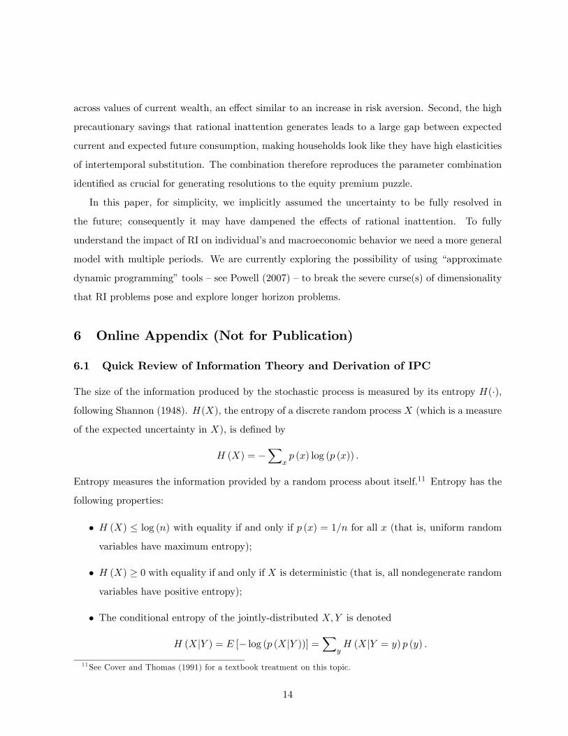
The size of the information produced by the stochastic process is measured by its entropy H(·),

following Shannon (1948). H(X), the entropy of a discrete random process X (which is a measure

of the expected uncertainty in X), is defined by

H (X) = −∑

xp (x) log (p (x)) .

Entropy measures the information provided by a random process about itself.11 Entropy has the

following properties:

• H (X) ≤ log (n) with equality if and only if p (x) = 1/n for all x (that is, uniform random

variables have maximum entropy);

• H (X) ≥ 0 with equality if and only if X is deterministic (that is, all nondegenerate random

variables have positive entropy);

• The conditional entropy of the jointly-distributed X,Y is denoted

H (X|Y ) = E [− log (p (X|Y ))] =∑

yH (X|Y = y) p (y) .

11See Cover and Thomas (1991) for a textbook treatment on this topic.

14

H (X|Y ) ≤ H (X) with equality if and only ifX and Y are independent (that is, conditioning

on a second random variable can never increase entropy);

• H (X,Y ) = H (X) +H (Y |X) = H (Y ) +H (X|Y ) ≤ H (X) +H (Y ) with equality if and

only if X and Y are independent (the joint entropy of two random variables is highest when

they provide no information about each other).

Mutual information is a measure of the information contained in one process regarding another

process. Suppose {X,Y } is a random process. The average mutual information between X and

Y is defined by

I (X;Y ) = H (X) +H (Y )−H (X,Y )

We can also write the mutual information in a more intuitive way using the conditional entropy

as

I (X;Y ) = H (X)−H (X|Y ) = H (Y )−H (Y |X) .

Both definitions are equivalent. Mutual information between the current consumption, savings

and the random vector of income in period 1 is given by

I(e1; c1, s

)= H

(e1)−H

(e1|c1, s

)or equivalently

I(e1; c1, s

)= H

(e1)+H

(c1, s

)−H

(e1, c1, s

).

According to the last property, the entropy of independent random variables is equal to the sum

of the entropy of each random variable. Thus we get

I(e1; c1, s

)= H

(e1)+H

(c1, s

)−H

(e1, c1, s

).

Writing the entropy explicitly yields

K∑k=1

N∑r=1

I∑i=1

f(sk, c

1r , e

1i

)log(f(sk, c

1r , e

1i

))−

I∑i=1

g1(e1i)log(g1(e1i))

(9)

−K∑k=1

N∑r=1

q(c1r , sk

)log(q(c1r , sk

)).

This expression is constrained to be smaller than the channel capacity, giving rise to (7). Since

entropy is a concave function, the resulting constraint set is convex.

15

6.2 Deriving First-order Conditions

The first-order conditions for f (·) ∈ (0, 1) are

Ukri − vi

1 + log

(f(sk,c1r,w1i )q(c1r,sk)

)− f(sk,c1r,w1i )

q(c1r,sk)

=Umns − vs

1 + log(f(sm,c1n,w

1s)

q(c1n,sm)

)− f(sm,c1n,w

1s)

q(c1n,sm)

for ∀k = 1, ...,K, r = 1, ..., N , and i = 1, ..., I, where

Ukri = u(c1r)+ β

D∑d=1

J∑j=1

u((w1i − c1r

) [sk

(red − rf

)+ rf

]+ e2j

)ϕ (red) g2

(e2j)

is the expected lifetime utility at the state with consumption c1r , the risky asset share sk, and

wealth w1i . The agent chooses optimal probabilities over different states such that the utility per

marginal mutual information are equated across different states.

Proposition 5 The agent allocates higher relative probability over the states with higher expected

utility if vi = vs.

Suppose vi = vs and Ukri > Umns. Then

f(sk, c

1r , w

1i

)q (c1r , sk)

− log(f(sk, c

1r , w

1i

)q (c1r , sk)

)<f(sm, c

1n, w

1s

)q (c1n, sm)

− log(f(sm, c

1n, w

1s

)q (c1n, sm)

).

Let ϕ (x) = x− log (x). Then Dϕ (x) < 0 if 0 < x < 1, sof(sk,c1r,w1i )q(c1r,sk)

>f(sm,c1n,w1s)q(c1n,sm)

.

16

References

[1] Bansal, Ravi and Amir Yaron (2004), “Risks for the Long Run: A Potential Resolution of

Asset Pricing Puzzles,”Journal of Finance 59, 1481-1509.

[2] Gabaix, Xavier and David Laibson (2001), “The 6D Bias and the Equity-Premium Puzzle,”

NBER Macroeconomic Annual 2001, 257-330.

[3] Gennotte, Gerard (1986), “Optimal Portfolio Choice under Incomplete Information,”Journal

of Finance 41, 733—749.

[4] Gomes, Francisco and Alexander Michaelides (2008), “Asset Pricing with Limited Risk Shar-

ing and Heterogeneous Agents,”Review of Financial Studies 21(1), 415-448.

[5] Guvenen, Fatih (2009), “A Parsimonious Macroeconomic Model for Asset Pricing,”Econo-

metrica 77(6), 1711-1750.

[6] Heaton, John and Deborah Lucas (2000), “Portfolio Choice in the Presence of Background

Risk,”Economic Journal 110: 1-26.

[7] Huang, Lixin and Hong Liu (2007), “Rational Inattention and Portfolio Selection,”Journal

of Finance 62(4), 1999-2040.

[8] Krusell, Per and Anthony A. Smith, Jr. (1997), “Income and Wealth Heterogeneity, Portfolio

Choice, and Equilibrium Asset Returns,”Macroeconomic Dynamics 1(2), 387-422.

[9] Lewis, Kurt F. (2009), “The Two-Period Rational Inattention Model: Accelerations and

Analyses,”Computational Economics 33(1), 79-97.

[10] Lundtofte, Frederik (2008), “Expected Life-time Utility and Hedging Demands in a Partially

Observable Economy,”European Economic Review 52(6), 1072-1096.

[11] Luo, Yulei (2010), “Rational Inattention, Long-run Consumption Risk, and Portfolio Choice,”

Review of Economic Dynamics 13(4), 843-860.

[12] Luo, Yulei and Eric R. Young (2010), “Risk-sensitive Consumption and Savings under Ra-

tional Inattention,”American Economic Journal: Macroeconomics 2(4), 281-325.

17

[13] Luo, Yulei and Eric R. Young (2014), “Long-run Consumption Risk and Asset Allocation

under Recursive Utility and Rational Inattention,”manuscript.

[14] Matejka, Filip and Christopher A. Sims (2010), “Discrete Actions in Information-Constrained

Tracking Problems,”manuscript.

[15] Merton, Robert C. (1969), “Lifetime Portfolio Selection under Uncertainty: The Continuous

Time Case,”Review of Economics and Statistics 51(1), 247-257.

[16] Mondria, Jordi (2010), “Portfolio Choice, Attention Allocation, and Price Comovement,”

Journal of Economic Theory 145(5), 1837—1864.

[17] Peng, Lin and Wei Xiong (2006), “Investor Attention, Overconfidence and Category Learn-

ing,”Journal of Financial Economics 80(3), 563-602.

[18] Powell, Warren B. (2007), Approximate Dynamic Programming: Solving the Curses of Di-

mensionality, Wiley Series in Probability and Statistics, John Wiley and Sons.

[19] Samuelson, Paul A. (1969), “Lifetime Portfolio Selection by Dynamic Stochastic Program-

ming,”Review of Economics and Statistics 51(3), 239-46.

[20] Shafieepoorfard, Ehsan and Maxim Raginsky (2013), “Rational Inattention in Scalar LQG

Control,”Proceedings of the IEEE Conference on Decision and Control 52, 5733-5739.

[21] Shannon, Claude (1948), “A Mathematical Theory of Communication,” The Bell System

Technical Journal 27, 623-56.

[22] Sims, Christopher A. (2003), “Implications of Rational Inattention,” Journal of Monetary

Economics 50(3), 665-90.

[23] Sims, Christopher A. (2005), “Rational Inattention: A Research Agenda,”Technical Report,

Princeton University.

[24] Sims, Christopher A. (2006), “Rational Inattention: Beyond the Linear-Quadratic Case,”

American Economic Review 96(2), 158-163.

[25] Tutino, Antonella (2012), “Rationally Inattentive Consumption Choices,” Review of Eco-

nomic Dynamics 16(3), 421-439.

18

[26] Wang, Neng (2009), “Optimal Consumption and Assets Allocation with Unknown Income

Growth,”Journal of Monetary Economics 56(4), 524-34.

[27] Van Nieuwerburgh, Stijn and Laura Veldkamp (2010), “Information Acquisition and Under-

Diversification,”Review of Economic Studies 77(2), 779-805.

19

Table 1: Expected Current and Future Consumption

γ = 0.5 γ = 2

E [c1] 0.0633 0.0624

E [c2] 0.0732 0.0742

Table 2: The Saving Rate under RI

κ ∞ 2 1 0.5 0.3 0.2 0.1 0.05

γ = 2 0.27 0.27 0.28 0.30 0.32 0.33 0.39 0.45

γ = 0.5 0.27 0.26 0.26 0.27 0.28 0.30 0.36 0.43

20

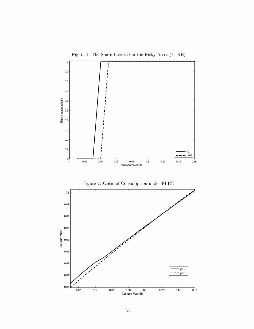
Figure 1: The Share Invested in the Risky Asset (FI-RE)

0 0.02 0.04 0.06 0.08 0.1 0.12 0.14 0.160

0.1

0.2

0.3

0.4

0.5

0.6

0.7

0.8

0.9

1

Current Wealth

Ris

ky a

sset

 sha

re

γ=2γ=0.5

Figure 2: Optimal Consumption under FI-RE

0.02 0.04 0.06 0.08 0.1 0.12 0.14 0.160.02

0.03

0.04

0.05

0.06

0.07

0.08

0.09

0.1

Current Wealth

Con

sum

ptio

n

γ=0.5γ=2

21

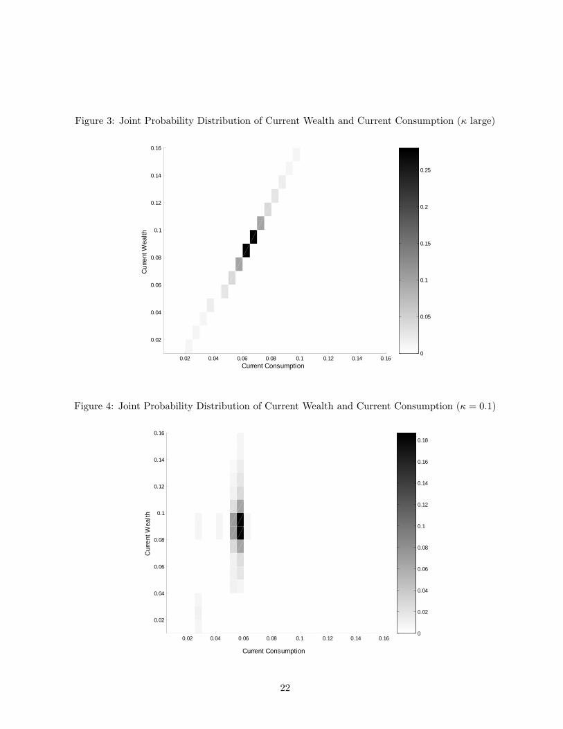
Figure 3: Joint Probability Distribution of Current Wealth and Current Consumption (κ large)

0.02 0.04 0.06 0.08 0.1 0.12 0.14 0.16

0.02

0.04

0.06

0.08

0.1

0.12

0.14

0.16

Current Consumption

Cur

rent

 Wea

lth

0

0.05

0.1

0.15

0.2

0.25

Figure 4: Joint Probability Distribution of Current Wealth and Current Consumption (κ = 0.1)

0.02 0.04 0.06 0.08 0.1 0.12 0.14 0.16

0.02

0.04

0.06

0.08

0.1

0.12

0.14

0.16

Current Consumption

Cur

rent

 Wea

lth

0

0.02

0.04

0.06

0.08

0.1

0.12

0.14

0.16

0.18

22

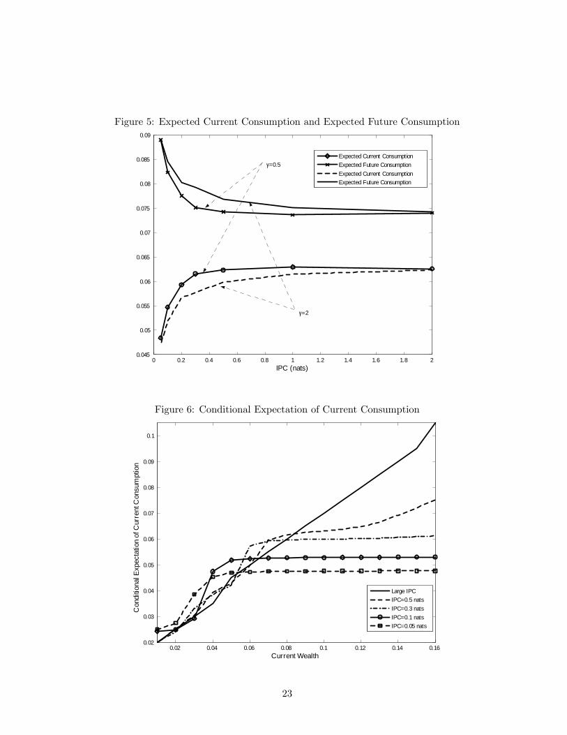
Figure 5: Expected Current Consumption and Expected Future Consumption

0 0.2 0.4 0.6 0.8 1 1.2 1.4 1.6 1.8 20.045

0.05

0.055

0.06

0.065

0.07

0.075

0.08

0.085

0.09

IPC (nats)

γ=0.5

γ=2

Expected Current ConsumptionExpected Future ConsumptionExpected Current ConsumptionExpected Future Consumption

Figure 6: Conditional Expectation of Current Consumption

0.02 0.04 0.06 0.08 0.1 0.12 0.14 0.160.02

0.03

0.04

0.05

0.06

0.07

0.08

0.09

0.1

Current Wealth

Con

ditio

nal E

xpec

tatio

n of

 Cur

rent

 Con

sum

ptio

n

Large IPCIPC=0.5 natsIPC=0.3 natsIPC=0.1 natsIPC=0.05 nats

23

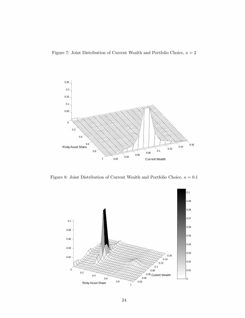
Figure 7: Joint Distribution of Current Wealth and Portfolio Choice, κ = 2

0

0.2

0.4

0.6

0.8

1 0.020.04

0.060.08

0.10.12

0.140.16

0.05

0.1

0.15

0.2

0.25

Current Wealth

Risky Asset Share

Figure 8: Joint Distribution of Current Wealth and Portfolio Choice, κ = 0.1

00.2

0.40.6

0.81

0.020.04

0.060.08

0.10.12

0.140.160.02

0.04

0.06

0.08

0.1

Current Wealth

Risky Asset Share0

0.01

0.02

0.03

0.04

0.05

0.06

0.07

0.08

0.09

0.1

24

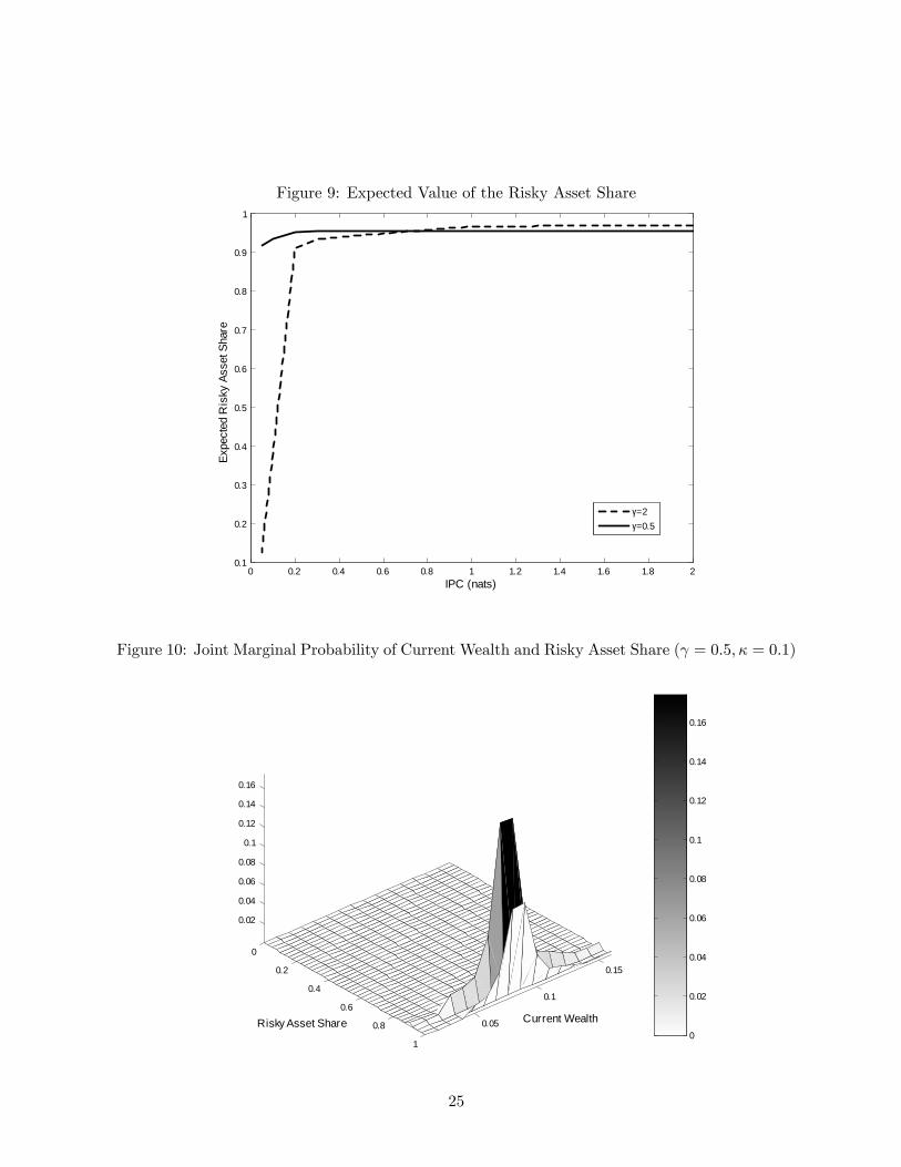
Figure 9: Expected Value of the Risky Asset Share

0 0.2 0.4 0.6 0.8 1 1.2 1.4 1.6 1.8 20.1

0.2

0.3

0.4

0.5

0.6

0.7

0.8

0.9

1

IPC (nats)

Expe

cted

 Ris

ky A

sset

 Sha

re

γ=2γ=0.5

Figure 10: Joint Marginal Probability of Current Wealth and Risky Asset Share (γ = 0.5, κ = 0.1)

0

0.2

0.4

0.6

0.8

1

0.05

0.1

0.15

0.02

0.04

0.06

0.08

0.1

0.12

0.14

0.16

Current WealthRisky Asset Share0

0.02

0.04

0.06

0.08

0.1

0.12

0.14

0.16

25

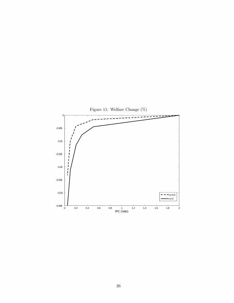
Figure 11: Welfare Change (%)

0 0.2 0.4 0.6 0.8 1 1.2 1.4 1.6 1.8 2­0.035

­0.03

­0.025

­0.02

­0.015

­0.01

­0.005

0

IPC (nats)

γ=0.5γ=2

26