The University of Melbourne

Department of Mathematics and Statistics

Polynomial Methods inCombinatorial Geometry

Kevin Scott Fray

Supervised by David Wood

Submitted in partial fulfillment of therequirements for the degree of

Master of Science

May, 2013

Contents

Abstract iii

1 The Erdos Distance Problem 1

2 Incidence Geometry 52.1 The distinct distances incidence problem . . . . . . . . . . . . . . . . . 52.2 The geometry of Elekes’ incidence problem . . . . . . . . . . . . . . . . 112.3 Ruled Surfaces . . . . . . . . . . . . . . . . . . . . . . . . . . . . . . . 14

3 Dvir’s Polynomial Method 173.1 The Polynomial Method . . . . . . . . . . . . . . . . . . . . . . . . . . 173.2 Properties of Polynomials . . . . . . . . . . . . . . . . . . . . . . . . . 183.3 Proof of the Finite Field Kakeya Conjecture . . . . . . . . . . . . . . . 213.4 Extensions to the Method . . . . . . . . . . . . . . . . . . . . . . . . . 22

4 The Joints Conjecture 244.1 Algebraic Tools . . . . . . . . . . . . . . . . . . . . . . . . . . . . . . . 244.2 The Joints Conjecture . . . . . . . . . . . . . . . . . . . . . . . . . . . 31

5 Polynomial Partitioning 345.1 The Szemeredi-Trotter Theorem . . . . . . . . . . . . . . . . . . . . . . 345.2 Decompositions of Space . . . . . . . . . . . . . . . . . . . . . . . . . . 365.3 Proof of the Szemeredi-Trotter Theorem via Polynomial Partitioning . 38

6 The Guth-Katz Proof 426.1 Proof of the k ≥ 3 case . . . . . . . . . . . . . . . . . . . . . . . . . . . 426.2 Proof of the k = 2 case . . . . . . . . . . . . . . . . . . . . . . . . . . . 486.3 Applications to arithmetic combinatorics . . . . . . . . . . . . . . . . . 51

7 The Dirac-Motzkin Conjecture 53

8 Extremal Examples 568.1 Projective Space . . . . . . . . . . . . . . . . . . . . . . . . . . . . . . 568.2 The Boroczky examples . . . . . . . . . . . . . . . . . . . . . . . . . . 59

i

8.3 The Sylvester Examples . . . . . . . . . . . . . . . . . . . . . . . . . . 628.4 An ‘Almost Group Law’ and the Boroczky examples . . . . . . . . . . . 63

9 Vanishing Polynomials 659.1 Melchior’s Inequality . . . . . . . . . . . . . . . . . . . . . . . . . . . . 659.2 Polynomials Vanishing on P . . . . . . . . . . . . . . . . . . . . . . . . 699.3 Reducing to a single cubic . . . . . . . . . . . . . . . . . . . . . . . . . 76

10 The Green-Tao proof 7910.1 Background Material . . . . . . . . . . . . . . . . . . . . . . . . . . . . 7910.2 The Green–Tao proof . . . . . . . . . . . . . . . . . . . . . . . . . . . . 80

11 Isosceles Triangles 8311.1 An upper bound by the polynomial method . . . . . . . . . . . . . . . 8411.2 Perpendicular bisectors . . . . . . . . . . . . . . . . . . . . . . . . . . . 86

Bibliography 88

ii

Abstract

Problems in combinatorial geometry (also called discrete geometry) concern the com-binatorial structure of discrete geometric structures. This thesis revolves around twoextremely classical problems, both concerning finite sets of points in the plane—Erdos’distinct distance problem and the ordinary line conjecture of Dirac and Motzkin. Re-cently, each of these problems has been almost resolved, the former by Guth and Katz[27] and the latter by Green and Tao [25]. Both proofs involve the study of algebraiccurves related to the geometric object, a technique that has come to be known as thepolynomial method. In this thesis we give a thorough exposition of the polynomialmethod in combinatorial geometry, motivated by the proofs of the results of Guth-Katzand Green-Tao. Along the way we will see the symbiotic relationship between combina-torial geometry and arithmetic combinatorics. Our original contribution is work on thetopic of isosceles triangles. We present several conjectures and a related new incidencebound.

iii

Chapter 1

The Erdos Distance Problem

Consider the following puzzle:

How can a farmer arrange his four farm buildings such that the distancebetween any two buildings is exactly 100m?

Equivalently, we are required to find a configuration of four points such that everypair is unit distance apart. The key to solving the puzzle is to realise that such aconfiguration does not exist—at least in the plane—the configuration we need is thevertices of a regular tetrahedron. The farmer must place (at least) one of the buildingson a hill or in a valley!

This puzzle is the simplest special case of an open question in the field of discretegeometry: precisely when do point sets with given distance distributions occur in theplane? More precisely, let P be a finite set of points in the plane, then the distancedistribution is the function DP : R≥0 → Z≥0 given by

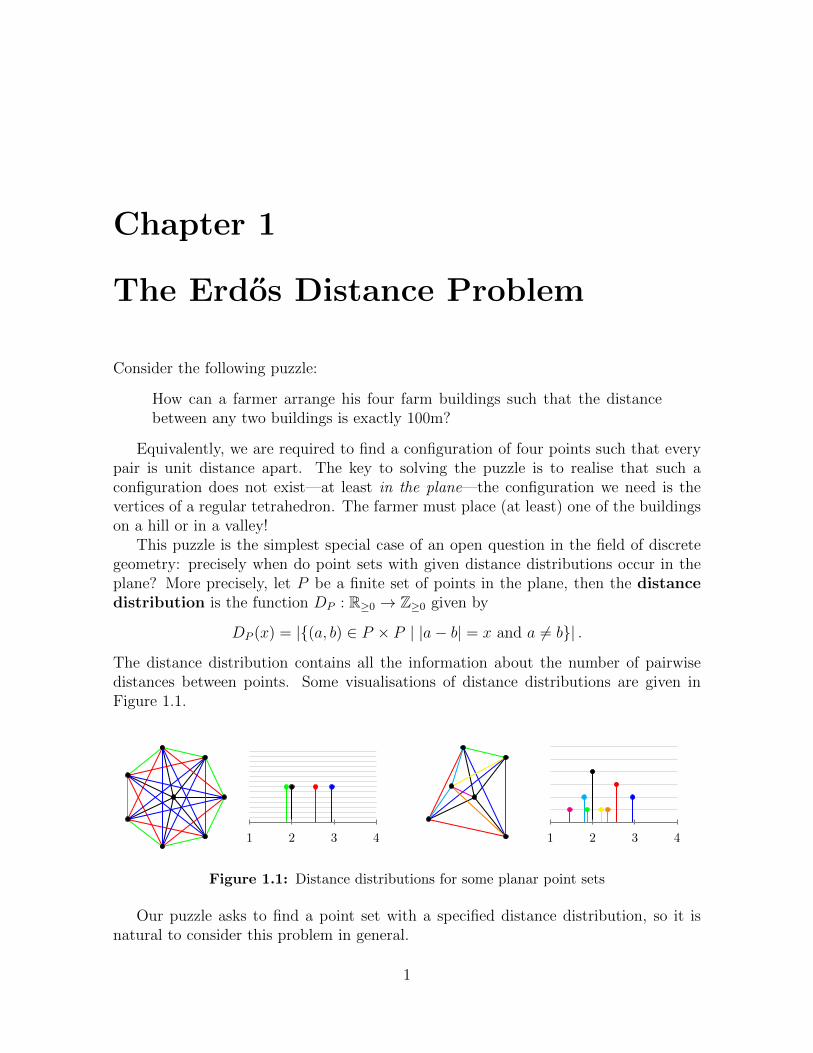
DP (x) = |{(a, b) ∈ P × P | |a− b| = x and a 6= b}| .The distance distribution contains all the information about the number of pairwisedistances between points. Some visualisations of distance distributions are given inFigure 1.1.

1 2 3 4 1 2 3 4

Figure 1.1: Distance distributions for some planar point sets

Our puzzle asks to find a point set with a specified distance distribution, so it isnatural to consider this problem in general.

1

Problem 1.1. Which functions D : R≥0 → Z≥0 arise as distance distributions of finitesets of points in the plane?

In general this problem is not well understood, and research has focused on specialcases. Note that since we are only interested in finite point sets, the distance distributionhas finite support. Hence it is natural to study the size of the support of DP , thenumber of distinct nonzero distances determined by P :

d(P ) = |{|a− b| | (a, b) ∈ P × P, a 6= b}| = |{x ∈ R | DP (x) 6= 0} \ {0}|

In particular, we are interested in the relationship between d(P ) and |P |. Trivially,since P determines only

(|P |2

)pairs at nonzero distance, d(P ) ≤

(|P |2

). Note that there

are point sets that achieve this upper bound—in fact almost all point sets have norepeated nonzero distances, so determine exactly

(|P |2

)distances. Also, d(P ) ≥ 1 when-

ever |P | ≥ 2 since there is at least one nonzero distance. We can restate the observationfrom the puzzle as the following

Proposition 1.2. Let P be a finite set of points in the plane. If d(P ) = 1 then |P | ≤ 3.

It is natural to wonder whether such a result always holds—given d(P ) can webound |P |, or can we find arbitrarily large point sets that determine a bounded numberof distances? To find a solution, consider again the puzzle. Suppose we have a set Pof four points in the plane such that each pair are unit distance apart. Choose two ofthese points, a and b. Consider the circle of unit radius centred at a. Any other pointof P is at unit distance from a and thus lies on this circle. The same holds for thecircle of unit radius centred at b, so the remaining two points must lie at the two pointsof intersection of these circles. The puzzle is now solved because these two points arenot at unit distance from each other, proving such a configuration does not exist in theplane.

Simply considering more than one distance in this argument, we obtain the followingresult first obtained by Erdos in 1944 (though his original proof was different, the proofwe give can be found in [24]).

Proposition 1.3 (Erdos, [19]). Let P be a finite set of points in the plane. Then1

|P | . d(P )2.

Proof. Let a, b be distinct points in P . Let Ca (resp. Cb) be the collection of d(P )circles centred at a (resp. b), with radii corresponding to the d(P ) distinct nonzerodistances determined by P . Every point of P \ {a, b} lies at an intersection point of acircle from Ca and a circle from Cb (Figure 1.2). Since two circles intersect in at mosttwo points, the number of such intersections is at most 2|Ca||Cb| = 2d(P )2. Therefore|P | − 2 = |P \ {a, b}| ≤ 2d(P )2.

1The notation f(n) . g(n) has identical meaning to f(n) ∈ O(g(n)), and is common in theliterature. We use this notation throughout.

2

a b

Ca Cb

Figure 1.2: Points of P lie at the intersection of two sets Ca and Cb of circles.

Rearranging gives the bound d(P ) & |P | 12 . That is, there do not exist arbitrarilylarge point sets that determine a bounded number of distances. Following on from thisresult, interest grew in trying to understand just how d(P ) grows with |P |. How smallcan d(P ) be when the size of |P | is fixed? Looking back to Figure 1.1 we see that apoint set determines few distances if it has a high degree of symmetry. In particular,consider the point set P given by the vertices of a regular n-gon. As shown for the casen = 16 in Figure 1.3, P determines d(P ) = bn

2c distances and one might conjecture

that such examples minimise d(P ) due to the high degree of symmetry.

1 2 3 4 5 6

(a) Distances in a regular 16-gon.

1 2 3 4 5

(b) Distances in a 4-by-4 square grid.

Figure 1.3: Distance distributions for highly symmetric point sets.

However, the regular n-gons do not minimise d(P )—consider the regular squaregrids {(a, b) | a, b ∈ Z and 1 ≤ a, b ≤ √n} for square n ≥ 1. The case n = 16 (a 4× 4grid) is shown in Figure 1.3. Although it determines more distances than the 16-gon, for√n ≥ 12 the

√n-by-

√n grid determines fewer distances than the corresponding n-gon.

As noted by Erdos, distances between points in the grid are of the form√x2 + y2 for

integer x, y, and so the number of distinct distances is at most the number of differentintegers at most 2n that have a representation of the form x2 + y2 for integer x, y. Thisquantity was studied by Landau [34] and is known to be . n/

√log n, thus the grids

asymptotically determine fewer distances than the regular n-gons. In Chapter 2 we willsee that this is a consequence of the grids having more ‘partial symmetries’ in a waythat will be made precise.

Erdos made the famous conjecture that the n-by-n grids do minimise d(P ), at leastasymptotically:

3

Conjecture 1.4 (Erdos’ Distinct Distances Conjecture, [19]). Let P be a finite set ofpoints in the plane. Then d(P ) & |P |/

√log |P |.

We have already seen Erdos’ 1946 result that d(P ) & |P | 12 . Gradually improvementsto this lower bound were discovered, including:

• d(P ) & |P | 23 in 1952 due to Moser [39];

• d(P ) & |P | 45 in 1992 due to Szekely [54];

• d(P ) & |P | 67 in 2001 due to Solymosi and Toth [51];

• d(P ) & |P |0.8641... in 2004 due to Katz and Tardos [32].

In November 2010, Larry Guth and Nets Katz posted to the arXiv ‘On the Erdosdistinct distance problem in the plane’ [27], in which they give the following almostoptimal result.

Theorem 1.5 (Guth-Katz, [27]). Let P be a finite set of points in the plane. Thend(P ) & |P |/ log |P |.

Their proof introduces new ideas from algebraic geometry that have begun to beused to approach many other problems in discrete geometry from a new perspective.In Chapters 2–6, we give an account of the new methods used in their proof, and theirrelationship to other problems in the field.

For background material on topics in combinatorial geometry, see Pach and Agar-wal [41] or Matousek [36]. Similarly for background on basic algebraic geometry seeBix [3] or Silverman and Tate [50] and for topics in arithmetic combinatorics see Taoand Vu [57].

4

Chapter 2

Incidence Geometry

We begin by remarking that the proof of Proposition 1.3 in the previous chapter isa corollary of an elementary incidence theorem—a result about the number of pointswhere a collection of geometric objects intersect.

Proposition 2.1. Distinct circles in the plane intersect in at most two points.

The proof is elementary, but for now we will not give it as we will find it is aconsequence of a very general result (Theorem 4.3) in Chapter 4. In general, incidenceproblems about lines, circles, points and higher dimensional varieties are widely studiedin combinatorial geometry. In this section we will give Elekes’ reduction ([17]) of theErdos distance problem to an incidence problem.

2.1 The distinct distances incidence problem

Recall the observation that point sets determining few distances possess a high degreeof symmetry (c.f. Figure 1.3). To study this carefully, we will consider the repeateddistances amongst the point sets. In particular, consider the collection of pairs of linesegments of the same length determined by a point set P , or equivalently the set ofquadruples formed by the endpoints of those segments:

Q(P ) = {(a, b, c, d) ∈ P 4 | |a− b| = |c− d| 6= 0}.

Note that Q(P ) contains the degenerate quadruples with {a, b} = {c, d}. If manysegments share the same length, the number of distinct distances should be small.Indeed, let d1, d2, . . . , dd(P ) be the distinct nonzero distances determined by P , and letni be the number of ordered pairs (a, b) ∈ P 2 satisfying |a − b| = di. Then by theCauchy-Schwarz inequality,

d(P )|Q(P )| = d(P )

d(P )∑i=1

n2i ≥

d(P )∑i=1

ni

2

= (|P |2 − |P |)2,

5

giving the bound

d(P ) ≥ |P |4 − 2|P |3|Q(P )| . (2.1)

Hence to estimate d(P ) it suffices to be able to estimate |Q(P )|.

PgP

g

a

b

c = ga

d = gb

(a) A quadruple (a, b, c, d) originates from an over-lap of P and gP .

P

gP

P∩ gP

(b) The one-to-one correspondence between di-rected segments in P ∩ gP and directed segmentsin g−1(P ∩ gP ).

Figure 2.1: Studying the repeated distances in terms of partial symmetries g. The point setP is illustrated with white circles, and the transformed point set gP is illustrated with filleddark circles.

Elekes’ idea was to transform the problem of estimating |Q(P )| into an incidenceproblem by looking at the symmetries of the point set P , or more specifically thepartial symmetries. That is, those rigid transformations g of the plane such that theimage gP intersects the point set P . So, let G be the group of orientation-preservingrigid motions of the plane—the translations and rotations. Then for a given quadruple(a, b, c, d) ∈ Q(P ) there is a unique transformation g ∈ G such that g(a) = c andg(b) = d — simply the composition of the translation sending a to c with a rotationabout c. Therefore we can define a map E : Q(P )→ G which takes each quadruple tothe corresponding unique g.

Proposition 2.2. Let P be a finite set of points in the plane. Then the functionE : Q(P )→ G given by

(a, b, c, d) 7→ the unique g ∈ G such that ga = c and gb = d

is well-defined.

A transformation g is called a partial symmetry of P if |P ∩ gP | ≥ 1. The map Eallows us to translate information about the partial symmetries of the point set P intoinformation about the set of quadruples Q(P ).

Lemma 2.3. Let P be a finite planar point set and let g ∈ G be an orientation-preserving rigid motion. If |gP ∩ P | = k then |E−1(g)| = k(k − 1).

6

Proof. If k = 0 then there is no a ∈ P with ga ∈ P and hence E−1(G) = ∅. Otherwiseassume k ≥ 1. Let gP ∩ P = {p1, . . . , pk}. For every i = 1, . . . , k we have pi = gqi forsome qi ∈ P . For each pair (pi, pj) ∈ (gP ∩ P )2 with pi 6= pj we have (qi, qj, pi, pj) ∈E−1(g) (as in Figure 2.1b, each such segment (pi, pj) gives a quadruple when takenwith its corresponding segment (qi, qj)). Since distinct pairs give distinct 4-tuples,|E−1(g)| ≥ k(k − 1). Conversely, if (a, b, c, d) ∈ E−1(g) then c = ga and d = gb, soc, d ∈ gP ∩ P (see Figure 2.1a). Hence |E−1(g)| = k(k − 1).

Lemma 2.3 shows that |Q(P )| = |E−1(G)| can be computed from the number ofpartial symmetries of the point set P . To give some notation for the number of partialsymmetries, let G=k(P ) = {g ∈ G | |gP ∩P | = k} be those partial symmetries of size k.Notice that by Lemma 2.3 partial symmetries g with k = 0 or k = 1 satisfy |E−1(g)| = 0.Hence by Lemma 2.3 we can count |Q(P )| in terms of the partial symmetries of size 2or greater,

|Q(P )| =|P |∑k=2

|G=k(P )|k(k − 1). (2.2)

(a) A rotation about a chord gives a partialsymmetry with k = 2.

(b) A rotation about the centre is a partialsymmetry with k = n (i.e. a full symmetry.)

Figure 2.2: Studying the repeated distances of ∆n in terms of partial symmetries g. Thepoint set ∆n is illustrated with white circles, and the transformed point set g∆n is illustratedwith filled dark circles.

Let us briefly return to look at the example of the regular n-gon ∆n from the pointof view of partial symmetries. Suppose g is a partial symmetry of ∆n. Any three pointsin general position in the plane determine a unique circle. Hence if |g∆n ∩ ∆n| ≥ 3,both ∆n and g∆n lie on the same circle, so coincide. Thus every partial symmetry hask = 2 or k = n (in which case it is a full symmetry.) One can check that the partialsymmetries g with k = 2 are precisely rotations about the centre of a chord followedby a rotation about the centre of ∆n (Figure 2.2a), and those with k = n are preciselythe rotations about the centre of ∆n (Figure 2.2b). That is, |G=2(∆n)| =

(n2

)n and

7

|G=n(∆n)| = n. By (2.2),

|Q(P )| = 2

(n

2

)n+ n(n− 1)n = 2n3 − 2n2.

Hence, by (2.1), d(P ) ≥ (n4−2n3)/(2n3−2n2) ≈ n/2. This is almost tight with the truevalue bn/2c because ∆n has distances almost uniformly distributed (c.f. Figure 1.3), soour usage of Cauchy-Schwarz in the derivation of (2.1) is almost tight.

For technical reasons we will see in Chapter 6, it is easier to estimate the sizesof the sets G≥k(P ) = {g ∈ G | |gP ∩ P | ≥ k} than the sets G=k(P ). Substituting|G=k(P )| = |G≥k(P )| − |G≥k+1(P )| into (2.2), we can estimate |Q(P )| in terms of thesesets,

|Q(P )| =|P |∑k=2

2|G≥k(P )|(k − 1). (2.3)

Recall that we ultimately want to transform the distinct distances problem intoan incidence problem. In particular, we want to relate the sets G≥k(P ) ⊂ G to theincidences of some family of structures inside G. Elekes’ idea was to consider thefamily of sets Sp,q = {g ∈ G | gp = q} of transformations taking p to q, for p, q ∈ P .Since transformations g ∈ G≥k(P ) take k′ points in P to k′ points in P for some k′ ≥ k,such g lie in at least k of the sets Sp,q.

Lemma 2.4. Let P be a finite planar point set and 2 ≤ k ≤ n. Then |G≥k(P )| isexactly the number of elements g ∈ G that are in at least k of the sets Sp,q for p, q ∈ P .

Proof. Let g ∈ G≥k(P ), and let gP∩P = {p1, p2, . . . , pk′} for some k′ satisfying k ≤ k′ ≤|P |. Further, since pi ∈ gP ∩P let pi = gqi for some qi ∈ P . Then for each i = 1, . . . , k′,g ∈ Sqi,pi . Hence g lies in at least k′ ≥ k of the sets Sp,q. Conversely, if g ∈ Sqi,pi fori = 1, . . . , k′ where k ≤ k′ ≤ |P |, then pi = gqi and hence pi ∈ gP ∩ P . If pi = pj thenqi = qj so Sqi,pi = Sqj ,pj , hence pi 6= pj whenever i 6= j. Thus |gP ∩ P | ≥ k′ ≥ k so bydefinition g ∈ G≥k(P ).

So, as desired, the quantities |G≥k(P )| are the solutions to an incidence problemabout the sets L = {Spq | p, q ∈ P}. If the bound |G≥k(P )| . |L|3/2/k2 holds then by(2.3),

|Q(P )| .|P |∑k=2

2|L|3/2(k − 1)/k2 ∼ |P |3 log |P |,

which by (2.1) gives the Guth-Katz result d(P ) & |P |/ log |P |.

Problem 2.5. Let P be a finite planar point set, and let L = {Sp,q ⊂ G | p, q ∈ p}. IfG≥k(P ) is the set of elements g ∈ G contained in at least k of the sets Sp,q ∈ L, howbig is |G≥k(P )|? In particular, is |G≥k(P )| . |L|3/2/k2?

8

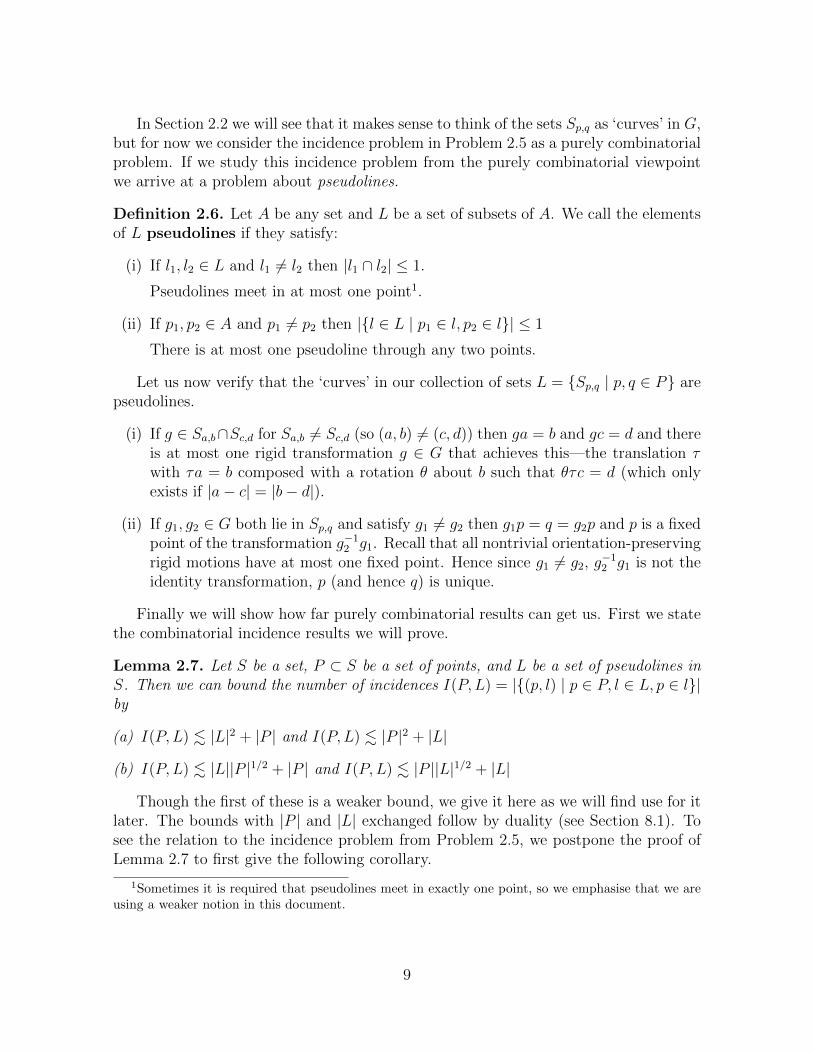
In Section 2.2 we will see that it makes sense to think of the sets Sp,q as ‘curves’ in G,but for now we consider the incidence problem in Problem 2.5 as a purely combinatorialproblem. If we study this incidence problem from the purely combinatorial viewpointwe arrive at a problem about pseudolines.

Definition 2.6. Let A be any set and L be a set of subsets of A. We call the elementsof L pseudolines if they satisfy:

(i) If l1, l2 ∈ L and l1 6= l2 then |l1 ∩ l2| ≤ 1.

Pseudolines meet in at most one point1.

(ii) If p1, p2 ∈ A and p1 6= p2 then |{l ∈ L | p1 ∈ l, p2 ∈ l}| ≤ 1

There is at most one pseudoline through any two points.

Let us now verify that the ‘curves’ in our collection of sets L = {Sp,q | p, q ∈ P} arepseudolines.

(i) If g ∈ Sa,b∩Sc,d for Sa,b 6= Sc,d (so (a, b) 6= (c, d)) then ga = b and gc = d and thereis at most one rigid transformation g ∈ G that achieves this—the translation τwith τa = b composed with a rotation θ about b such that θτc = d (which onlyexists if |a− c| = |b− d|).

(ii) If g1, g2 ∈ G both lie in Sp,q and satisfy g1 6= g2 then g1p = q = g2p and p is a fixedpoint of the transformation g−12 g1. Recall that all nontrivial orientation-preservingrigid motions have at most one fixed point. Hence since g1 6= g2, g

−12 g1 is not the

identity transformation, p (and hence q) is unique.

Finally we will show how far purely combinatorial results can get us. First we statethe combinatorial incidence results we will prove.

Lemma 2.7. Let S be a set, P ⊂ S be a set of points, and L be a set of pseudolines inS. Then we can bound the number of incidences I(P,L) = |{(p, l) | p ∈ P, l ∈ L, p ∈ l}|by

(a) I(P,L) . |L|2 + |P | and I(P,L) . |P |2 + |L|

(b) I(P,L) . |L||P |1/2 + |P | and I(P,L) . |P ||L|1/2 + |L|

Though the first of these is a weaker bound, we give it here as we will find use for itlater. The bounds with |P | and |L| exchanged follow by duality (see Section 8.1). Tosee the relation to the incidence problem from Problem 2.5, we postpone the proof ofLemma 2.7 to first give the following corollary.

1Sometimes it is required that pseudolines meet in exactly one point, so we emphasise that we areusing a weaker notion in this document.

9

Corollary 2.8. Let S be a set and L be a set of pseudolines in S. Then we can boundthe size of the set of incidences I≥k(L) = |{p ∈ S | p ∈ l1, l2, . . . , lk′ for some k′ > k}|of at least k pseudolines in L by

(a) |I≥k(L)| . |L|2

kand (b) |I≥k(L)| . |L|

2

k2

Proof. We only prove (a) as the deduction of (b) is the same, simply using Lemma 2.7(b)rather than Lemma 2.7(a). Set P = I≥k(L). By Lemma 2.7(a) applied to P and L,

|P |k ≤ I(P,L) . |L|2 + |P |.

That is, |P |(k − 1) . |L|2 and hence |I≥k(L)| = |P | . |L|2/k.

(a) An arrangement of pseudolines, with in-tersection points illustrated.

(b) The collinearity graph for the pseudolinearrangement. Edges between adjacent verticeson the pseudolines are lightened for clarity.

Figure 2.3: The construction of the collinearity graph of an arrangement of pseudolines.

Proof of Lemma 2.7. Let L = L≤1 ∪ L≥2 where L≤1 consists of the lines containing atmost one point of P and L≥2 those containing at least two points. Thus I(P,L) =I(P,L≤1) + I(P,L≥2). First note that I(P,L≤1) ≤ |L≤1| ≤ |L|.

To bound I(P,L≥2), construct the collinearity graph of G with vertices V = P andan edge p1 ∼ p2 if there is a pseudoline l ∈ L with p1 ∈ l and p2 ∈ l. This constructionis illustrated in Figure 2.3. Each edge p1 ∼ p2 is associated to a unique l ∈ L since twopoints determine at most one pseudoline, so this construction produces a graph ratherthan a multigraph.

Proof of (a). Since each edge corresponds to at most two incidences, I(P,L≥2) ≤2|E(G)|. Also |E(G)| ≤

(|P |2

)≤ |P |2 since |V | = |P |. Thus

I(P,L) ≤ I(P,L≤1) + I(P,L≥2) ≤ |L|+ 2

(|P |2

). |L|+ |P |2.

10

Proof of (b). Let l1, . . . , l|L| be the pseudolines in L, and let ni be the number of pointsof P on line li. Line li contributes

(ni

2

)edges to G, so

|L|∑i=1

(ni2

)= |E(G)| ≤

(|P |2

)and hence

|L|∑i=1

(ni − 1)2 ≤ |P |2.

Applying Cauchy-Schwarz,

I(P, I≥2(L)) =∑ni≥2

ni ≤ |L|+|L|∑i=1

(ni − 1) ≤ |L|+ |L|1/2 |L|∑

i=1

(ni − 1)2

12

≤ |L|+ |L|1/2|P |.

Therefore I(P,L) ≤ I(P,L≤1) + I(P,L≥2) . |L|+ |L|1/2|P |.

To see how far these purely combinatorial techniques have propelled us, we substi-tute the bound Corollary 2.8(b), into (2.3) to get

|Q(P )| .|P |∑k=2

2|L|2k2

(k − 1) ≈ |P |4 log |P |,

recalling that our incidence problem involves |L| = |P |2 pseudolines. This bound on thenumber of quadruples implies (by (2.1)) the (very underwhelming) bound d(P ) & 1

log |P | .As far as solving our incidence problem, this is as far as purely combinatorial techniquescan take us, since the bound (b) is tight for pseudolines. For example take P to be ann × n grid in the plane and L to be the 2n horizontal and vertical lines through thegrid — the number of incidences is I(P,L) = 2n2 ≈ |L||P |1/2 + |L|.

In the next section, we find that to resolve our incidence problem we need to exploitadditional geometric structure—the structure of the group G of transformations andthe structure of our collection of ‘curves’ Sp,q.

2.2 The geometry of Elekes’ incidence problem

In the previous section we saw Elekes’ transformation of the distinct distances problemto an incidence problem in the group G of rigid orientation-preserving transformationsof the plane. To have a hope of solving this incidence problem, we need to understandthe geometry of the ‘curves’ Sp,q whose intersections we wish to understand. In thissection we will give Guth and Katz’ observation [27, Section 2] that we can furtherreduce to an incidence problem about lines in R3.

First, we note that almost all transformations g ∈ G are rotations, so it is notunreasonable to expect that also most incidences occur at rotations. It turns out thisis in some sense correct, since it is easy to bound the number of incidences occurring

11

at translations. To see this, let Grot consist of the rotations g ∈ G, and Gtrans consistof the translations. Then G = Grot ∪ Gtrans and in an analogous way we decomposeG≥k(P ) = Grot

≥k(P ) ∪Gtrans≥k (P ).

As hoped, the number of incidences at translations obeys the desired bound fromProblem 2.5.

Lemma 2.9. |Gtrans≥k (P )| . |L|3/2/k2.

Proof. Let Qtrans(P ) consist of those quadruples in Q(P ) arising from translations. If(a, b, c, d) ∈ Qtrans(P ) then d = c+ (b− a), so that d is determined from a, b, c. Hence|Qtrans(P )| ≤ |P |3 = |L|3/2. By the derivation of (2.2), we can restrict (2.2) to justtranslations,

|L|3/2 ≥ |Qtrans(P )| =|P |∑i=2

i(i− 1)|Gtrans=i (P )| ≥ k(k − 1)|Gtrans

≥k (P )|,

that is, |Gtrans≥k (P )| . |L|3/2/k2 as desired.

Having dealt with translations, we can turn to understanding the incidences atrotations. The advantage of isolating the rotations is that the geometry is far easier tounderstand. Any planar rotation g is a rotation around some fixed point f = (fx, fy)by an angle θ. Hence the space has a natural parameterisation2 η : Grot → R2× (0, 2π)taking g 7→ (fx, fy, θ). To understand the incidences of the sets Spq in Grot, we can studythe incidences of the images η(Spq ∩Grot) in the much more familiar space R2× (0, 2π).

As first noticed by Guth and Katz [27], this parameterisation is especially simple ifwe ‘stretch’ it to fill R3 appropriately. Specifically, define ρ : Grot → R3 by

ρ(g) = (fx, fy, cotθ

2) (2.4)

for fx, fy, θ as above. Amazingly, by stretching the parameterisation in this way theimages Lp,q = ρ(Spq ∩Grot) becomes lines.

Proposition 2.10. If p = (px, py) and q = (qx, qy) are points in R2 then the set Lp,q isa line in R3.

Proof. Consider any g ∈ Spq ∩ Grot. As in Figure 2.4, let m = (p + q)/2 denote themidpoint of pq and let f be the fixed point of g on the perpendicular bisector of p and q.We will only give the proof in the general case p 6= q and f 6= m—the degenerate casesare similar and simpler. We have cot θ

2= ||f−m||||p−m|| . Let us write f = m+ f−m

||f−m|| ||f −m||,and note that

||p−m|| f −m||f −m|| =

(qy − py

2,px − qx

2

).

2The original parameterisation proposed by Elekes considered g as a rotation by θ about the originfollowed by a translation by (x, y), and parameterised g by g 7→ (x, y, θ). Unfortunately the images ofthe Sp,q under this parameterisation are helices in R2 × (0, 2π) and proved difficult to understand.

12

f

p

q = gp

mθ2

g

Figure 2.4: Computing the angle of rotation of the rotation taking p to q.

Hence

ρ(g) =

(fx, fy,

||f −m||||p−m||

)=

(px + qx

2,py + qy

2, 0

)+||f −m||||p−m||

(qy − py

2,px − qx

2, 1

).

As g ranges over all rotations taking p to q, ||f−m||||p−m|| assumes all values in R, so that

Lpq =

{(px + qx

2,py + qy

2, 0

)+ t

(qy − py

2,px − qx

2, 1

): t ∈ R

}(2.5)

is indeed a line.

Redefining our notation from before (pg. 8), we will now let L = {Lpq | p, q ∈ P}be the set of lines in R3. Since we have removed a point (the translation) from each ofour curves, we first verify that they are still distinct.

Proposition 2.11. |L| = |P |2

Proof. Let La,b and Lc,d be two lines in L. Again we just give the argument in thegeneral case a 6= b and a 6= c, since similar arguments work in the degenerate cases.Let g be the rotation by 180 ◦ around the midpoint of a and b, so g ∈ Sab. If g 6∈ Scd weare done, since the lines do not share the point ρ(g), so are distinct. Otherwise c andd lie on the line ab. For any other rotation g′ ∈ Sab, g′ 6∈ Scd since a is the only pointon ab for which g′(a) is also on ab, and we have assumed c 6= a.

We have seen that our main problem can be transformed into an incidence problemabout |P |2 lines in R3. It makes sense, then, to wonder in what generality this incidenceproblem holds. Will the desired bound hold for an arbitrary set of lines in R3.

Problem 2.12. Let L be a finite set of lines in R3. If I≥k(L) is the set of pointsin R3 contained in at least k of the lines l ∈ L, how big is I≥k(L)? In particular, is|I≥k(L)| . |L|3/2/k2?

13

Unfortunately, examples exceeding this bound are easy to construct. For instance,consider the case where all lines of L lie in a plane, with no two parallel. Since eachpair intersects, there are |I≥2(L)| & |L|2 intersections of k = 2 or more lines. Similarlyfor k = 3 one could take the lines L to form a finite section of a triangular lattice, sothat |I≥3(L)| & |L|2. Fortunately, the special properties of the lines Lpq rule these sortsof examples out for the lines we are looking at.

Proposition 2.13. Lpq and Lpq′ are disjoint and have different directions if q 6= q′.

Proof. If g ∈ Lpq ∩ Lpq′ then q′ = g(p) = q, so the lines are disjoint. By the pa-rameterisation of Lpq in (2.5), if they have the same direction then ( qy−py

2, px−qx

2, 1) =

λ(q′y−py

2, px−q

′x

2, 1) so λ = 1. This implies qy − py = q′y − py so qy = q′y. Similarly,

px − qx = px − q′x so qx = q′x. That is, q = (qx, qy) = (q′x, q′y) = q′.

Corollary 2.14. At most |L|1/2 = |P | lines of L lie in a given plane π.

Proof. By Proposition 2.13, if two lines Lp,q and Lp,q′ were contained in π then theywould intersect. However, these lines are disjoint as one cannot simultaneously havep = gq and p = gq′. Hence for each p ∈ P there is at most one q ∈ P such that Lp,q ⊂ π,so π contains at most |P | lines of L.

Having ruled out this instance, one would again ask whether Problem 2.12 holds inthe restricted case where at most |L|1/2 lines lie in any one plane. Yet again it turnsout that this is not the case—if our lines L all lie in a doubly ruled surface, with halfof the lines in each ruling, then again |I≥k(L)| & |L|2. However since the only k-ruledsurface for k ≥ 3 is the plane, these types of exceptions don’t exist for k ≥ 3. In fact,Guth and Katz proved the following incidence theorem.

Theorem 2.15 (Guth-Katz, [27, Proposition 2.11]). Let L be a finite set of lines inR3 for which no more than |L|1/2 lie in a common plane, and let 3 ≤ k ≤ |L|1/2. Then|I≥k(L)| . |L|3/2/k2.

In the next section we will investigate the exceptional examples lying in ruled sur-faces that arise in the k = 2 case.

2.3 Ruled Surfaces

We now turn to the theory of ruled surfaces. We give the relevant results without proof,though the interested reader shall find an exposition in [27, Section 3]. A more throughtreatment of the theory of ruled surfaces is available in [47, Chapter XIII, Part 3]. Thefundamental definition is:

Definition 2.16. Let S ⊂ R3 be an algebraic surface, and k ≥ 1. We say S is k-ruled if through every point on S there are k distinct lines which are contained inthe surface S. A 1-ruled surface is called singly-ruled and a 2-ruled surface is calleddoubly-ruled.

14

We give special names to the k = 1, 2 cases because the only surface which is 3-ruled, or k-ruled for any k ≥ 3, is a plane (sometimes the plane is called ∞-ruled).Non-planar examples are given by a cylinder or a cone, both of which are singly ruled,or a hyperboloid of one sheet which is doubly-ruled (these examples are illustrated inFigure 2.5.) Other examples are given by reguli.

Figure 2.5: The singly-ruled cone and cylinder and a doubly-ruled hyperboloid. Some linescontained in each of the surfaces are shown.

Definition 2.17. An algebraic surface S ⊂ R3 is a regulus if there are three pairwiseskew lines l1, l2, l3 such that S is the union of the family of lines that intersect all threelines l1, l2, and l3.

It is not obvious, but any choice of three pairwise skew lines gives a regulus by thisconstruction (that is, the union S is an algebraic surface). For example, in Figure 2.6a regulus has been constructed from the three lines

l1 = {(−1, t, 0) | t ∈ R}, l2 = {(0, s, s) | s ∈ R}, l3 = {(1, 0, r) | r ∈ R}.

The family of lines intersecting all three lines l1, l2, and l3 is the family of lines connecting(−1, t, 0), (0, t/2, t/2), and (1, 0, t) for each t ∈ R. The corresponding regulus S isdoubly-ruled, for instance the point (−1, t, 0) ∈ l1 is contained in the aforementionedline as well as the line l1 itself. In fact, every regulus is doubly-ruled, and moreover wehave now seen all doubly-ruled surfaces.

Proposition 2.18 (Classification of Ruled Surfaces, [47]). Let S ⊂ R3 be an irreducibleruled surface. Then exactly one of the following holds

(i) S is a plane and S is k-ruled for every k ≥ 3;

(ii) S is a regulus and S is doubly-ruled;

(iii) S is singly-ruled.

15

Figure 2.6: Example of a regulus determined by the three highlighted lines l1, l2, l3. Weshow some of the lines in each direction of the ruling, and the surface formed by the union oflines intersecting all of l1, l2, and l3.

Returning to our incidence problem, we have an analogous result to Corollary 2.14for reguli.

Lemma 2.19 ([27, Proposition 2.8]). The number of lines of L lying in a given regulusS is . |L|1/2.

In an analogous way to Theorem 2.15, it turns out that the plane and reguli examplesare the only examples contradicting the incidence theorem for k = 2.

Theorem 2.20 (Guth-Katz, [27, Proposition 2.10]). Let L be a finite set of lines in R3

for which at most |L|1/2 lie in a common plane, and . |L|1/2 lie in a common regulus.Then |I≥2(L)| . |L|3/2.

So far, we have seen Elekes’ reduction of the Erdos distinct distances problem to anincidence problem and how by studying the geometry of the resulting problem, Guthand Katz isolated the properties of the incidence problem that give the desired boundsin Theorem 2.15 and Theorem 2.20. In Chapters 3–6 we introduce the polynomialmethod and show how it has been used by Guth and Katz to prove these two bounds.

16

Chapter 3

Dvir’s Polynomial Method

In 2008, Dvir solved the long outstanding finite field Kakeya problem with a remarkablysimple argument exploiting the behaviour of polynomials. His proof introduced alge-braic ideas that are the core of Guth and Katz’ bound on the Erdos distinct distancesproblem. In this section we will present his use of what is now called the polynomialmethod to solve this problem. To begin with, we define the finite-field Kakeya problem.

Problem 3.1. Let F be a finite field. Call a set K ⊂ Fn a Kakeya set if it contains aline in every direction—that is, for every direction x ∈ Fn there is a line {y+tx | t ∈ F}contained in K. What is the minimum size of a Kakeya set?

This problem was first considered by Wolff [58], as a simpler version of the (stillopen) problem for infinite fields, which instead considers sets containing line segmentsin every direction. Prior to Dvir’s work, the lower bound was conjectured to be & |F|nbut the strongest known bound was just & |F|4n/7 due to Rogers [46]. In 2008, Dvir [13]proved this conjecture with a remarkably simple proof using the polynomial method,even obtaining a respectable estimate of the constant in the bound.

3.1 The Polynomial Method

We begin by defining the basic object of study in the polynomial method.

Definition 3.2. Let p ∈ F[x1, . . . , xn] be a polynomial. The degree of p is the largestvalue of a1 + · · · + an for all monomials xa11 x

a22 · · ·xann in p. The zero set of p is

Z(p) = {x ∈ Fn | p(x) = 0}.The zero set of p depends on the ring we consider p to be a member of. For instance,

Z(x) = {0} if we consider x to belong to the ring F[x], while Z(x) = {(0, y) | y ∈ F}if we consider x to belong to the ring F[x, y]. Whenever we refer to Z(p) the ring inquestion will be clear from context. We also remark that where we will use degree someauthors prefer total degree; we use the former since it is the only concept of degree thatwe use. Similarly we use the term zero set where others may find variety or algebraiccurve/surface more familiar.

17

The essence of the polynomial method is studying a combinatorial structure byrelating it to the zero set Z(p) of some polynomial p. In the applications we will see,the procedure is as follows.

(i) We have a finite set S in some field Fn and we want to bound its size.

(ii) Find a nonzero polynomial p ∈ F[x1, . . . , xn] with S ⊂ Z(p) of ‘small’ degree.

(iii) Use the properties of the set S together with the low degree of the polynomial pto conclude that S cannot be contained in Z(p), a contradiction.

Intuitively, the polynomial method works because the ‘complexity’ of Z(p) is closelyrelated to the degree of p. If one can use the properties of S to conclude it is more‘complex’ than Z(p), one can arrive at a contradiction. We will see how this outlineis implemented in Dvir’s resolution of the finite-field Kakeya conjecture, but first wemust give some basic results about polynomials that allow us to achieve (ii) and (iii).

3.2 Properties of Polynomials

Remarkably, step (ii) is often achieved with a general polynomial existence result, ratherthan by using the structure of S to construct a polynomial. Thinking about this problemin dimension n = 1, the obvious construction is to take the product

p(x) =∏s∈S

(x− s)

giving a polynomial with S ⊂ Z(p) of degree d = |S|. The natural generalization to 2-dimensions is to again let p be the product of linear factors, so that the zero set of eachfactor is a line. One can choose these lines to vanish on at least 2 points of S, giving apolynomial of degree d = d |S|

2e. Similarly in n dimensions, the analogous construction

gives a polynomial of degree d = d |S|ne. For applications, this naıve approach is much too

weak—using only linear factors is far too restrictive. A much more efficient approachis available, using simple linear algebra.

Lemma 3.3. Let F be any field and S ⊂ Fn a finite set. Then there is a nonzeropolynomial vanishing on S of degree d . |S|1/n, where the hidden constant depends onn (or precisely, of any degree d such that

(n+dd

)> |S|).

Proof. Consider a general polynomial p(x1, . . . , xn) of degree d. It has(n+dd

)coefficients.

For each s = (s1, . . . , sn) ∈ S, we have the linear equation p(s1, . . . , sn) = 0 in the(n+dd

)coefficients. Taking all of these |S| equations, we see that there is a nonzero polynomialof degree d vanishing on S if and only if this system has a nonzero solution. Hencewe have a solution whenever

(n+dd

)> |S|. Rearranging, we will have a solution with

d . |S|1/n where the hidden constant depends on n.

18

This takes care of constructing vanishing polynomials. To carry out (iii), one tech-nique is to show that our polynomial is in fact zero, contradicting that we constructeda nonzero polynomial. To show that the polynomial is zero, we have several standardresults that can show if a polynomial vanishes in one place is must vanish in another.The first of these is the familiar result that a nonzero degree d polynomial has at mostd zeros.

Proposition 3.4. Let F be a field and p ∈ F[x] be a nonzero polynomial of degree d.Then |Z(p)| ≤ d.

Proof. Simply apply the fact that if p(a) = 0 then (x− a) divides p (a consequence ofdivision of polynomials, since if p(x) = (x−a)q(x)+r(x) then 0 = p(a) = (a−a)q(a)+r(a) = r(a)).

This proposition is usually used in its contrapositive form, to conclude that a poly-nomial is zero because it vanishes in too many places. We also remark that for finitefields, we cannot use the proposition in this way for polynomials of degree |F| or more,since there are not |F|+ 1 points at which the polynomial vanishes.

From this, we can derive the following lemma that implements the concept thatlow-degree polynomials have ‘simple’ zero-sets.

Lemma 3.5. Let F be a field and p ∈ F[x1, . . . , xn] be a nonzero polynomial of degreed. Also, let L = {y+ tx | t ∈ F} ⊂ Fn be a line in Fn. If |Z(p)∩L| > d then L ⊂ Z(p).(That is, any line not contained in Z(p) intersects Z(p) in at most d points.)

Proof. The restriction of p to L is p0(t) = p(y+ tx), a single-variable polynomial in F[t]of degree at most d which has at most d zeros from Proposition 3.4.

Figure 3.1: The curve Z(y − (x − 3)(x − 1)(x + 1)(x + 3)) meets each of the dashed linesin at most four points.

An example in the plane is shown in Figure 3.1, for the curve y = (x−3)(x−1)(x+1)(x + 3). In this planar case, Lemma 3.5 is a generalisation of Proposition 3.4 whichsimply counts intersections with the line y = 0.

In infinite fields analogous results to Proposition 3.4 do not hold for multivariatepolynomials, since Z(p) is always infinite. However, in finite fields the Schwartz-Zippellemma extends Proposition 3.4.

19

Lemma 3.6 (Schwartz-Zippel lemma, [49, 59]). Let F be a finite field and p ∈ F[x1, . . . , xn]be a nonzero polynomial of degree d. Then |Z(p)| ≤ d|F|n−1.

Proof. We proceed by induction on n. The n = 1 case is Proposition 3.4. Otherwisen > 1. Considering p as an element of (F[x2, . . . , xn])[x1],

p(x1, . . . , xn) =r∑i=1

gi(x2, . . . , xn)xi1,

where r is such that gr is a nonzero polynomial of degree at most d − r. Then byinduction, |Z(gr)| ≤ (d− r)|F|n−2. For any zero (a1, . . . , an) ∈ Z(p), we must have thata1 is a zero of the single variable polynomial p0(x1) = p(x1, a2, . . . , an). Hence we cancount the zeros in two cases

Case 1: If (a2, . . . , an) ∈ Z(gr) then p0 could be zero, so |Z(p0)| ≤ |F|.

Case 2: If (a2, . . . , an) 6∈ Z(gr) then p0 is nonzero of degree r, so |Z(p0)| ≤ r.

Combining,

|Z(p)| ≤ |F||Z(gr)|+ r|Fn−1 \ Z(gr)|≤ (d− r)|F|n−1 + r|F|n−1≤ d|F|n−1.

Clearly we cannot bound the number of points in the same way for an infinite field,but we do have the simple result that if p 6= 0 there is some point not in Z(p).

Lemma 3.7. Let F be an infinite field and p ∈ F[x1, . . . , xn] be a nonzero polynomialof degree d. Then |Fn \ Z(p)| ≥ 1.

Proof. We proceed by induction on n, noting that the case n = 1 follows immediatelyfrom Proposition 3.4. Suppose p ∈ F[x1, . . . , xn]. Cconsidering p as an element of(F[x1, . . . , xn−1])[xn], it has only finitely many roots, so there is some a ∈ F suchthat 0 6= p(x1, . . . , xn−1, a) ∈ F[x1, . . . , xn−1]. Applying the induction hypothesis, thispolynomial does not vanish everywhere so we are done.

It turns out this is enough to prove another useful result which bounds the ‘com-plexity’ of zero sets in a certain sense.

Lemma 3.8. Let F be a field and p ∈ F[x, y] be a nonzero polynomial of degree d.

(a) If F is finite and d < |F| then Z(p) contains at most d distinct lines.

(b) If F is infinite then Z(p) contains at most d distinct lines.

Proof. Suppose for contradiction that Z(p) contains d+ 1 distinct lines. Now either

20

(a) F is finite, so apply Lemma 3.6 to conclude that p does not vanish identically andhence find a 6∈ Z(p). Since there are d + 1 ≤ |F| lines in Z(p), there is a linel through a not parallel to any of these lines (since lines in F2 can have |F| + 1different directions.)

(b) F is infinite, so apply Lemma 3.7 to conclude that p does not vanish identically andhence find a 6∈ Z(p). Choose a line l through a that is not parallel to any of thed+ 1 lines contained in Z(p).

The line l intersects all d + 1 of the lines in Z(p) and hence is contained in Z(p) byLemma 3.5. This is a contradiction, since p does not vanish at a.

Readers familiar with algebraic geometry may like to note that over an algebraicallyclosed field Lemma 3.8 is a consequence of the Nullstellensatz (since if Z(ax+by) ⊂ Z(p)then ax + by divides p), and indeed over R the result follows from similarly generalstatements from real algebraic geometry (see [5, Section 4]).

3.3 Proof of the Finite Field Kakeya Conjecture

Before we give Dvir’s full proof of the finite field Kakeya conjecture, we first give anintuitive proof for the planar case. To the author’s knowledge this simple method ofproof is original, although the planar case is of little independent interest since theplanar result was known even in Wolff’s original paper [58].

Proposition 3.9. Let F be a finite field, and K ⊂ F2 a Kakeya set. Then |K| & |F|2.

Proof. Suppose K is a Kakeya set with |K| . |F|2. By Lemma 3.3 there is a nonzeropolynomial p vanishing on K of degree d . |F|. By choosing a small enough hiddenconstant in the statement of the theorem, we in fact have d < |F|. Since K is a Kakeyaset, it contains at least |F|+ 1 distinct lines, one in each of the |F|+ 1 directions (theyare distinct since they are in different directions.) This is a contradiction, since Z(p)should contain at most d ≤ |F| − 1 distinct lines, by Lemma 3.8.

We obtain an intuitive contradiction by ‘complexity’: a Kakeya set must contain aline in every direction, so cannot be placed inside a zero set of a ‘low degree’ polynomial,and hence the Kakeya set must be ‘big’.

We are now ready to give Dvir’s proof in full detail. Dvir’s original proof uses aclosely related concept to Kakeya sets, which we briefly define.

Definition 3.10. Let F be a finite field. A set N ⊂ Fn is a Nikodym set if throughevery y 6∈ N there is a line through y which lies otherwise entirely in N , that is{y + tx | t ∈ F∗} ⊂ N for some x ∈ Fn.

The first simpler version of Dvir’s argument does not prove the full Kakeya conjec-ture, but was still groundbreaking.

21

Theorem 3.11 ([13, Theorem 1]). Let F be a finite field, and K ⊂ Fn a Kakeya set.Then |K| & |F|n−1 where the hidden constant depends on n.

Proof. Suppose for contradiction that K is a Kakeya set with |K| . |F|n−1. Then theset N = FK is a Nikodym set, since given y 6∈ N we can choose a line {x+ ty | t ∈ F}in the direction y contained in K, and then {sx+ sty | s ∈ F, t ∈ F} is contained in N .In particular, {sx+y | s ∈ F∗} is contained in N . We have |N | . |F|n so by Lemma 3.3there is a nonzero polynomial p vanishing on N of degree d . |F|. With a small enoughhidden constant, d ≤ |F| − 2. Then for any point y 6∈ N , p vanishes on the |F| − 1 > dpoints {sx + y | s ∈ F∗}. Hence p vanishes at the remaining point y on this line, byLemma 3.5. That is, p vanishes everywhere and so must be the zero polynomial (bythe Schwartz-Zippel Lemma) contradicting our choice of p.

The proof of Theorem 3.11 arrives at a contradiction by exploiting the high ‘com-plexity’ of the Nikodym set—having a line through every external point that is otherwisecontained in the set. Following the preprint of Dvir’s work, Alon and Tao found analternative approach that exploited the complexity of the Kakeya set itself, to give atighter bound.

Theorem 3.12 ([13, Theorem 3]). Let F be a finite field, and K ⊂ Fn a Kakeya set.Then |K| & |F|n where the hidden constant depends on n.

Proof. The proof uses ideas from projective space, which we review in Section 8.1.Suppose for contradiction that K is a Kakeya set with |K| . |F|n. As in the previousproof, by Lemma 3.3 we can find a nonzero polynomial p vanishing on K of degreed < |F|. Now embed K into projective space PFn and consider the homogenisation ofp given by ph(x0, . . . , xn) = xd0p(x1/x0, . . . , xn/x0). Since K is a Kakeya set, throughevery point a = [0, a1, . . . , an] on the hyperplane at infinity there is a line L ⊂ K inthe direction a. This line contains |F| points of K so by Lemma 3.5, ph vanishes at a.That is, ph vanishes at every point on the hyperplane at infinity. However, ph restrictedto the line at infinity is just ph(0, x1, . . . , xn) which is the highest degree homogeneouspart of p. This is a contradiction since we assumed p was nonzero of degree d < |F|, soit cannot vanish identically by the Schwartz-Zippel Lemma (Lemma 3.6).

The proof of Theorem 3.12 exploits the complexity of the Kakeya set K to concludethat any polynomial vanishing on K must vanish on the hyperplane at infinity, whichis a copy of PFn−1. Since we can not find a ‘low’ degree polynomial vanishing on thisspace, we can not find a ‘low’ degree polynomial vanishing on K, so K is big.

3.4 Extensions to the Method

Following the work of Dvir, refinements to the polynomial method have been used toimprove Theorem 3.12. Saraf and Sudan [48] used the concept of the multiplicity ofa zero to get a tighter bound on the size of Kakeya sets. Recall that in the single-variable case, the polynomial p(x) = (x− a)k has a zero of order k at a. In general, a

22

polynomial p(x1, . . . , xn) has a zero of multiplicity k at (a1, . . . , an) if every monomialin p(x1 +a1, . . . , xn +an) has degree at least k. By finding analogues of Lemma 3.3 andLemma 3.5 for general multiplicities, Saraf and Sudan improved Theorem 3.12. Thisidea has come to be known as the method of multiplicities.

With some additional improvements, Dvir et al. [14] obtained the current bestbound, tight to within a small constant factor.

Theorem 3.13 ([14, Theorem 11]). Let F be a finite field, and K ⊂ Fn a Kakeya set.Then |K| ≥ 1

(2−1/|F|)n |F|n.

The ideas were also extended by Ellenberg, Oberlin and Tao [18] to solve a relatedproblem. If F is a finite field and S ⊂ Fn then S is a k-plane if S is a translation ofa k-dimensional subspace of Fn. A subset K ⊂ Fn is a k-plane Kakeya set if for everyk-dimensional subspace V of Fn, there is a k-plane contained in K which is a translationof V . We note that by an induction argument, Lemma 3.8 can be generalised to boundthe number of (n−1)-planes contained in Z(p) ⊂ Fn when p ∈ F[x1, . . . , xn]. Using this,the same proof as Lemma 3.3 bounds the size of (n− 1)-plane Kakeya sets. Ellenberg,Oberlin and Tao obtained a strong bound in the general k case.

Theorem 3.14 ([18, Proposition 4.16]). Let F be a finite field and K ⊂ Fn a k-plane

Kakeya set where 2 ≤ k < n. Then |K| ≥ (1− |F|1−k)(n2)|F|n.

So far we have seen the successful application of the polynomial method to problemsover finite fields. As we will see, the method has much wider applicability, althoughit remains to be seen whether the method of multiplicities can be applied in othercontexts. In the next section we will see how the polynomial method can be applied toproblems over Rn.

23

Chapter 4

The Joints Conjecture

After Dvir’s work, Guth and Katz [26] successfully applied the polynomial method tothe joints problem, an incidence problem in real space. The joints problem is a simplerversion of the incidence problem in Theorem 2.15 for the case k = 3, and the proof ofthe joints conjecture introduced many elements that were eventually used in the fullproof of Theorem 2.15. In this chapter we give the proof of the joints conjecture.

Definition 4.1. Let L be a set of lines in R3. A point p of R3 is called a joint of L ifthere are three lines in L which meet at p and do not all lie in a plane.

The work of Guth and Katz [26] resolved the joints conjecture of Chazelle et al. [6],obtaining the following tight bound.

Theorem 4.2. Let L be a set of lines in R3 and let J be the set of joints of L. Then|J | . |L|3/2.

Prior to the application of the polynomial method to the problem by Guth andKatz, the best known bound was |J | . |L|1.6232, obtained by Feldman and Sharir [21].Guth and Katz’ motivation for studying the joints problem was the connection withthe real Kakeya problem. We will study this proof as a stepping stone to the resolutionof the Erdos distinct distances problem, but the reader interested in the connectionsto the Kakeya problem should consult [43]. Several different simplifications to Guthand Katz original proof have appeared [42, 16, 31]. We follow the proof of [16], andin particular we give their generalisation of the proof to ‘flat’ points, a case which iscrucial for the resolution of the Erdos distinct distances conjecture.

4.1 Algebraic Tools

Most of our algebraic results are corollaries of Bezout’s famous theorem on the numberof incidences between algebraic curves in the plane.

Theorem 4.3 (Bezout’s Theorem). If p, q ∈ R[x, y] have degrees dp and dq respectivelyand have no common factors, then |Z(p) ∩ Z(q)| ≤ dpdq.

24

Figure 4.1: Z(y2 − x) and Z(y − 100(x− 1)(x− 2)(x− 3)) meet in six points.

For example, if q is of degree 1 then Z(q) is a line, and for any polynomial p ∈R[x, y] this line intersects Z(p) in at most dp points. This is the planar case of ourvery first lemma on the complexity of zero sets, Lemma 3.5. Figure 4.1 illustrates anexample where p = y2 − x and q = y − 100(x − 1)(x − 2)(x − 3) are of degree 2 and3 respectively, and we see that the two curves Z(p) and Z(q) intersect in 6 points. Asanother application, we can quickly obtain the result of Proposition 2.1 (two circlesintersect in at most two points) by applying a planar inversion1 at a point on one ofthe circles, giving a line and a circle which by Bezout’s theorem intersect in at mosttwo points.

For application to the joints problem, we will use the following proposition whichleverages Bezout’s theorem up to dimension 3.

Proposition 4.4. If p, q ∈ R[x, y, z] have degrees dp and dq and have no commonfactors then there are at most dpdq lines contained in Z(p) ∩ Z(q).

For instance, if p and q are products of linear factors then Z(p) and Z(q) are unionsof planes. In the general case where none of these planes are parallel and no 3 intersectalong a line, we get dpdq lines contained in Z(p) ∩ Z(q) from each choice of a planein Z(p) and a plane in Z(q), so this proposition is tight. Both Bezout’s theorem andProposition 4.6 can be proven using the theory of resultants; we will not give theseproofs but they can be found in [26, Corollary 2.3] and [16, Proposition 1].

The proof of the joints conjecture via the polynomial method involves finding avanishing polynomial p on the set of lines L, and observing that the joints are ‘special’points of Z(p). To that end we introduce the following definitions.

Definition 4.5.

1. A point a ∈ Z(p) is critical for p if ∇p(a) = 0.

2. A point a ∈ Z(p) is regular for p if ∇p(a) 6= 0 (i.e. if it is not critical.)

1Viewing elements of R2 as elements of C∪{∞}, inverting the plane at the point a means to applythe map 1

z−a , sending the point ∞ to a and sending a to ∞. One can check that circles through amap to lines and other circles remain circles after applying inversion, and that inversion preserves theincidence structure.

25

3. A line l ⊂ Z(p) is a critical line for p if every point in l is critical for p.

Intuitively, we can think of critical points as points where two irreducible compo-nents of Z(p) meet. For instance, if p = xy ∈ R[x, y, z] then Z(p) is the union of theplanes x = 0 and y = 0, and ∇p = (y, x, 0) = 0 exactly on the line x = y = 0 where thetwo planes meet. In general, ∇p is normal to the surface Z(p), and where two distinctirreducible components of Z(p) meet there is no nonzero normal vector, so ∇p = 0.

Notice that the we define critical lines as lines contained in the zero set of the twopolynomials p and the three polynomials ∇p. Looking at Proposition 4.4, the followingresult should not be surprising.

Proposition 4.6. Let p ∈ R[x, y, z] be square-free of degree d. Then Z(p) contains atmost d(d− 1) critical lines for p.

Proof. If p is irreducible then p and ∂p∂x

have no common factors, and the partial deriva-tive has degree d − 1, so from Proposition 4.4, Z(p) contains at most d(d − 1) criticallines for p. The case where p is reducible involves induction on the degree; details aregiven in [16, Proposition 3].

To see why square-free polynomials must be excluded, consider the example p =x2 ∈ R[x, y, z], where ∇p = (2x, 0, 0). In this example, any line contained in the planex = 0 is a critical line.

In addition to critical points where two components of the surface meet, we willhave to deal with a second special type of point.

Definition 4.7.

1. A regular point a ∈ Z(p) is linearly flat for p if there are three distinct linesl1, l2, l3 ⊂ Z(p), each containing a.

2. A regular point a ∈ Z(p) is flat for p if the second fundamental form of Z(p)vanishes at a.

3. A line l ⊂ Z(p) is a flat line for p if all but finitely many points in l are flatpoints for p.

Readers not familiar with the second fundamental form can find details in [12],although Proposition 4.13 gives an equivalent definition of flat points without referenceto the second fundamental form. If we let p = xy ∈ R[x, y, z] as before then anya ∈ Z(p) \ (Z(x) ∩ Z(y)) is linearly flat, since there are three lines containing a inwhichever of the planes Z(x) or Z(y) contains a. The line l = {(0, y, 1) | y ∈ R} is aflat line for p since (0, 0, 1) is the only critical point in l.

We will need to understand the relationship between flat lines and the irreduciblecomponents of Z(p). In particular we have the following result.

Proposition 4.8. If p = fg ∈ R[x, y, z] and l ⊂ Z(p) is a flat line for p, then l is aflat line for either f or g.

26

Since the second fundamental form is defined locally, Proposition 4.8 is not surprising—whether a point is flat is determined only by the component Z(f) or Z(g) in which thepoint sits. At the intersection of Z(f) and Z(g) the points are critical, so are of noconcern in determining whether a line is flat.

If the second fundamental form vanishes at a regular point a ∈ Z(p) then locally ata, Z(p) is part of a plane, so Z(p) is indeed ‘flat’. The following proposition justifiescalling linearly flat points ‘flat’.

Proposition 4.9. Let a ∈ Z(p) and suppose there are three distinct lines l1, l2, l3 ⊂Z(p), which each contain a. If a is a regular point then the three lines are coplanar. Ifthe three lines are noncoplanar, then a is a critical point.

Proof. We only prove the latter statement as it is the contrapositive of the first. Weuse the argument from Kaplan, Sharir and Shustin [31]. Let u1 be a unit vector inthe direction of l1, so that l1 = {a + tu1 | t ∈ R}. Then taking a first order Taylorapproximation,

p(a+ tv) = p(a) + t∇p · u1 +O(t2).

But p(a + tv) = p(a) = 0 for all t ∈ R, so by taking t small enough we conclude∇p · u1 = 0. However, repeating for l2 and l3 we get

∇p · u1 = ∇p · u2 = ∇p · u3 = 0

where u2, u3 are unit vectors in the directions of l2 and l3 respectively. However, sincethe lines are noncoplanar, these three directions span R3, so∇p = 0 and a is critical.

This justifies the use of the term linearly flat, as a linearly flat point must be themeeting point of three lines lying in a plane in Z(p). Indeed, linearly flat points areflat in the sense of Definition 4.7.

Proposition 4.10 ([16]). A linearly flat point is flat.

We are especially interested in linearly flat points as they are the flat points that areeasiest to work with. In Proposition 4.6, we were able to control the number of criticallines in Z(p) by using the fact that ∇p characterises the critical points. It is not soobvious that there are polynomials that characterise flat points in this way. Guth andKatz’ original construction ([26]) used nine polynomials, we instead use the constructionof Elekes, Kaplan and Sharir [16] of three polynomials characterising linearly flat points.

Definition 4.11. Let e1, e2, e3 ∈ R3 denote the standard unit vectors in the x, y, zdirections. The Hessian of p is

Hp =

pxx pxy pxzpxx pxy pxzpxx pxy pxz

.

Define Πi(p) ∈ R[x, y, z] for i = 1, 2, 3 by

Πi(p) = (∇p× ei)THp(∇p× ei)and denote Π(p) = (Π1(p),Π2(p),Π3(p)).

27

Since the degrees of the polynomials in ∇p are dp− 1 and the degrees of the secondderivatives in the Hessian are dp − 2, the degrees of the polynomials Π(p) are 3dp − 4.We will not prove the following, but these polynomials characterise flat points in thefollowing sense.

Proposition 4.12. Let p ∈ R[x, y, z], and a ∈ Z(p). Then a is flat if and only ifΠ(p)(a) = 0.

We note that we can use this to prove Proposition 4.10 by first checking that thesecond order Taylor approximation to Z(p) vanishes on the three lines through a, andnoticing that it also vanishes at a general line in the tangent plane at a since the Taylorapproximation has degree 2 and already vanishes at the three points where the linemeets l1, l2 and l3. Thus we are in the same situation as for critical lines, where flatlines are lines contained in the intersection of two zero sets, of Z(p) and of Z(Πi(p)) forsome i = 1, 2, 3.

Proposition 4.13 ([16]). Let p ∈ R[x, y, z] be square-free of degree d with no linearfactors. Then Z(p) contains at most d(3d− 4) flat lines for p.

Again we defer to the proof in [16, Proposition 7]. Intuitively for an irreduciblepolynomial, if we have too many flat lines then p divides each Πj, so that every regularpoint is a flat point—but that means that Z(p) is a plane!

To find critical and flat lines in Z(p), we will require the following statements relatingthem to critical and flat points.

Proposition 4.14.

1. A line l ⊂ Z(p) containing more than d − 1 critical points of Z(p) is a criticalline for p.

2. A line l ⊂ Z(p) containing more than 3d− 4 linearly flat points of Z(p) is a flatline for p.

Proof. Both statements follow from Lemma 3.5 since if px vanishes at more than d−1 =deg (px) points or Π1(p) vanishes at more than 3d− 4 = deg (Π1(p)) flat points (we usethat linearly flat points are flat) then px (or Π1(x) respectively) vanishes identically onl. Hence by definition l is a critical line or l is a flat line.

We choose to state the second statement for linearly flat points as this is the versionwe will use, though one could as well state it for flat points. Finally, combining all ofthese results gives a statement about the complexity of collections of lines contained inZ(p) which meet in a lot of places.

Proposition 4.15. Let p ∈ R[x, y, z] be a square-free polynomial of degree d and letL be a collection of lines contained in Z(p). Let J be the set of points where are leastthree lines of L meet, and suppose that

28

(i) no plane contains more than B lines of L;

(ii) every line l ∈ L contains more than 4d points of J .

Then |L| ≤ 4d2 +Bd.

Proof. Let l ∈ L. Any point where two other lines of L meet l is either a critical pointor a linearly flat point, by Proposition 4.9. Since l contains more than 4d such points,it either contains more than d critical points or more than 3d linearly flat points, so iseither a critical or flat line by Proposition 4.14. So every line in l is critical or flat forp.

Write p = π1 · · · πkp for some k ≤ d where each πi is a linear factor and p has nolinear factors. Every line l ∈ L is either critical or flat for p, and a flat line for p is aflat line for one of the factors π1, · · · , πk, p by Proposition 4.8. Now we can bound thenumber of lines in L by observing:

• Z(p) contains at most d2 critical lines by Proposition 4.6;

• Z(πi) contains at most B lines by assumption, so in particular contains at mostB flat lines, for each i = 1, . . . , k;

• Z(p) contains at most 3d2 flat lines by Proposition 4.13.

Since every line in L is of one of these types,

|L| ≤ d2 +Bk + 3d2 ≤ 4d2 +Bd.

Proposition 4.14 controls the number of lines in terms of the degree of the surface,the number of lines in any given plane and crucially the line-line incidences amongstthe collection of lines. We now have the tools to understand the collection of linescontained in the zero set of a polynomial. To apply these tools, it will be convenientto isolate some particular ways to apply Lemma 3.3 to place a given set of lines insidethe zero set of a polynomial. The simplest method is the following.

Lemma 4.16. Let L ⊂ Rn be a finite set of lines. Then there is a nonzero polynomialp of degree d . |L|1/(n−1) such that every line l ∈ L is contained in Z(p).

Proof. For each line l ∈ L choose C|L|1/(n−1) points in Rn which lie on l, where C isa constant to be fixed later. This gives a total of C|L|n/(n−1) points, so by Lemma 3.3there is a nonzero polynomial p vanishing at these points of degree d . C1/n|L|1/(n−1).By choosing C large enough we have d < C|L|1/(n−1), so by Lemma 3.5 every line l ∈ Lis contained in Z(p), as desired.

For some applications, however, we will be concerned with a family L of lines whichintersect often. It turns out that in this situation, a more powerful result is available.The following proof is implicit in [26, 16].

29

Lemma 4.17. Let C & 1 be a constant and let L ⊂ Rn be a finite set of lines with|L| & 1 and satisfying:

(i) every line l ∈ L contains at least C|L|1/(n−1) points lying on other lines in L.

Then there is a nonzero polynomial p of degree d . 1C1/(n−1) |L|1/(n−1) such that every

line l ∈ L is contained in Z(p).

Proof. Take a random subset L′ ⊂ L by choosing each line independently with proba-bility 1

C.

Claim. With positive probability,

(1) 1 ≤ 12C|L| ≤ |L′| ≤ 2

C|L| and

(2) every line l ∈ L contains at least 12|L|1/(n−1) points lying on lines in L′.

To see this, first recall Chernoff’s bounds (see [2]) which we use in the form

P

[m∑i=1

Yi ≥ mp+mε

]≤ exp (−2ε2m), P

[m∑i=1

Yi ≤ mp−mε]≤ exp (−2ε2m)

whenever Yi are independent Bernoulli random variables with P [Yi = 1] = p. To applyChernoff’s bounds we set L = {l1, . . . , l|L|} and rephrase the claims (1) and (2) in termsof the indicator variables 1li∈L′ , giving:

• P [A] = P [∑|L|

i=1 1li∈L′ ≥ 2C|L|] ≤ exp (−2|L|/C2);

• P [B] = P [∑|L|

i=1 1li∈L′ ≤ 12C|L|] ≤ exp (−1

2|L|/C2);

• For each l ∈ L, let Ll = {ln1 , . . . , lnk} ⊂ L be a set of distinct lines each incident

to a distinct point on L, with k ≥ C|L|1/(n−1) by the assumption (i). ThenP [Cl] = P [

∑ki=1 1lni∈L′ ≤

12|L|1/(n−1)] ≤ exp (−1

2|L|1/(n−1)/C).

Putting them together, by the union bound

P [A ∪B ∪⋃l∈L

Cl] ≤ exp (−2|L|/C2) + exp (−1

2|L|/C2) +

∑l∈L

exp (−1

2|L|1/(n−1)/C)

and since we have |L| & 1 and C & 1 by choosing these constants appropriately, wewill have P [A ∪B ∪⋃l∈LCl] < 1, so with positive probability (1) and (2) hold.

Now by Lemma 4.16 we can find a polynomial p vanishing on L′ of degree d .1

C1/(n−1) |L|1/(n−1). Since each line of L contains at least 12|L|1/(n−1) points lying on lines

in L′, and this can be made larger than d by ensuring C is large enough, we have byLemma 3.5 that each line of L is in Z(p).

30

4.2 The Joints Conjecture

We can now give the slick proof of the joints conjecture. We give the proof by Kaplanet al. [31], which somewhat simplifies the original proof by Guth and Katz [26].

Theorem 4.2. Let L be a set of lines in R3 and let J be the set of joints of L. Then|J | . |L|3/2.

Proof. We proceed by induction on |L|. For clarity, let the hidden constant in thestatement be A so we wish to prove that |J | ≤ A|L|3/2. For |L| less than some fixedlarge constant we obtain the result by taking a large enough implicit constant in thestatement, since trivially |J | ≤ |L|2. For the induction step assume for the sake ofcontradiction that we have a set L of n lines and a set J as specified, and such that|J | > A|L|3/2.

We first prune L by iteratively removing any line from L that contains fewer thanC|L|1/2 points and removing the corresponding points from J (here C is a constantwhich we will fix later, and this threshold C|L|1/2 stays fixed as we remove lines fromL). This gives us a subset L′ ⊂ L and its set of joints J ′ which satisfy:

(i) every line of L′ is incident to at least C|L|1/2 joints of L′;

(ii) |J ′| ≥ |J | − C|L|3/2 (since we removed at most C|L|3/2 points in this process).

Case 1. If |L′| < |L|/2 then applying induction to L′ we get

|J ′| ≤ A|L′|3/2 < A/2|L|3/2.

HenceA|L|3/2 < |J | ≤ |J ′|+ C|L|3/2 < (A/2 + C)|L|3/2,

a contradiction since we can take A with A/2 ≥ C.

Case 2. Otherwise, |L′| ≥ |L|/2. By Lemma 4.17 we can find a square-free polynomial pwhich vanishes on every line in L′ and by appropriate choice of C, has degree d ≤ 1

2|L|1/2.

By Proposition 4.9 (and that the three lines at any joint are noncoplanar) each jointis a critical point for p. Hence since each line contains at least C|L|3/2 joints each linein L is critical by Proposition 4.14. However, by Proposition 4.6 the number of criticallines is at most d2 ≤ |L|/4, a contradiction.

In either case, we reach a contradiction.

Amazingly, the results about critical lines do most of the work for us. The remainingwork of the proof is just checking the easier case when there are lines not containingmany joints!

Elekes, Kaplan and Sharir [16] observed that the proof of the Joints conjecture couldbe altered to bound the number of incidences with points that are ‘flat’ joints, wherethe three incident lines are coplanar. This was a crucial step towards the resolution

31

of the Erdos distinct distances conjecture as the incidence problem is of this form. Tocontrol the number of these flat points, an assumption about the number of points orlines lying in any given plane is required (recall that in the distinct distances incidenceproblem, we can bound the number of lines in any given plane or regulus.)

Theorem 4.18 ([16, Theorem 9]). Let L be a set of at most n lines in R3 and let Pbe a set of m arbitrary points in R3 such that:

(i) no plane contains more than Bn points of P , where B is an absolute constant;

(ii) each point of P is incident to at least three lines of L.

Then m ≤ An3/2 for some absolute constant A.

Proof. Set ε = 10−8 and c = 1020. We can take A such that

A ≥ max{100c,√Nε,c} = max{1022,

√Nε,c}.

We proceed by induction on n. If n ≤ Nε,c then m ≤ n2 ≤√Nε,cn

3/2 ≤ An3/2.We suppose for contradiction that |L′| = n and |P ′| = m satisfy the assumptions, butm > An3/2.

While there is a line in L′ incident to fewer than cn1/2 points of P ′, remove thatline and the incident points from L′ and P ′, and call the resulting sets L and P . Thisremoves at most cn3/2 points of P ′, so |P | ≥ |P ′| − cn3/2. These sets satisfy that

(i) no plane contains more than |L|1/2 ≤ n1/2 points of P

(ii) each point of P is incident to at least three lines of L

(iii) each line of L is incident to at least cn1/2 points of P

Suppose |L| < n100

. Set L0 = L and P0 = P . Iteratively, if there is a plane π

containing more than√|Li| lines then remove the lines and points from that plane to

form Li+1 and Pi+1. This process takes at most 2n1/2 steps. A point is in P \Pk comeseither from the intersection of two lines in L \ Lk or from a line in Lk with a line inL \ Lk. There can be at most 2n3/2 of the first kind since L \ Lk consists of at most2n1/2 planes each containing at most n1/2 lines, so each plane has at most n internalintersections and each pair of planes has at most 2n points of incidence on their line ofintersection. We also have at most n3/2 of the second kind since a line of Lk does notlie in any plane and so intersects each of the n1/2 planes at most once. Lastly by theinduction hypothesis, |Pk| ≤ A|Lk|3/2 ≤ A

100n3/2. Hence

(A− c)n3/2 ≤ |P ′| − cn3/2 ≤ |P | ≤ 2n3/2 + n3/2 +A

100n3/2

which is a contradiction since A > 10099

(3 + c).

32

Otherwise |L| ≥ n100

. Since 1 > ε > 0 and c > 3000ε−2, by a careful examination ofthe constants we can apply Lemma 4.17 to P and L to get a polynomial p of degreed ≤ εn1/2 which vanishes on the lines of L. Applying Proposition 4.15, since no planecontains more than n1/2 lines of L, we have

|L| ≤ 4d2 + n1/2d ≤ (4ε2 + ε)n

which is a contradiction since 4ε2 + ε < 1100

.

In this chapter, we have seen how the polynomial method can be used to provean incidence problem with many of the features of Guth and Katz’ Theorem 2.15.The proof of Theorem 2.15 combines the tools we have seen so far with another newidea: polynomial partitioning. In Chapter 5 we introduce the method of polynomialpartitioning, the last tool needed to give the bound on the Erdos distinct distancesproblem.

33

Chapter 5

Polynomial Partitioning

We have already seen how the polynomial method can be used to solve incidence prob-lems by placing a combinatorial structure inside a low degree algebraic surface andarguing that this surface is ‘simple’ in an appropriate sense. One of the breakthroughsof Guth and Katz was to realise that polynomials could be used to replace a classicaltool in combinatorial geometry – space decompositions. In this section we will see boththe classical tool of cell decompositions and Guth and Katz’ polynomial partitions, andtheir relationship.

5.1 The Szemeredi-Trotter Theorem

We will use the famous Szemeredi-Trotter theorem to introduce the method of polyno-mial partitioning. The theorem improves upon the weak purely combinatorial boundswe have seen in Lemma 2.7 to give an optimal bound for incidences between points andlines in R2.

Theorem 5.1 (Szemeredi-Trotter, [55]). Let P ⊂ R2 be a finite planar point set andL be a finite set of lines. Recall the definition of the number of point-lines incidences,I(P,L) = |{(p, l) | p ∈ P, l ∈ L, p ∈ l}|. Then

I(P,L) . |P |2/3|L|2/3 + |P |+ |L|. (5.1)

To see that the bound is optimal, consider the grid P = {1, 2, . . . , n}×{1, 2, . . . , 2n2}with the collection of lines L of the form lm,c = {(t,mt+ c) | t ∈ R} for m ∈ {1, . . . , n}and c ∈ {1, . . . , n2}. We have |P | = 2n3, |L| = n3 and lm,c ∩ P = {(t,mt + c) |t ∈ {1, . . . , n}} has size n, so that I(P,L) = n4 ∼ |P |2/3|L|2/3. As we have seen whenstudying Lemma 2.7, the other terms in (5.1) can also be dominant for certain examples.

Theorem 5.1 was originally proved by Szemeredi and Trotter [55] by an argumentusing a decomposition of space into squares. Later we will see a simpler proof in thisstyle, but first we will look at the beautiful modern proof given by Szekely [54]. Themain ingredient of this proof is the crossing number inequality.

34

Theorem 5.2 (Crossing Number Inequality, [1, 35]). Suppose G = (V,E) is a graphwith a drawing in the plane. Denote by cr(G) the number of crossings in the drawing(the number of points where a pair of edges intersect, excluding intersections at vertices).If |E| ≥ 4|V | then

cr(G) &|E|3|V |2 . (5.2)

Proof. Recall that a planar graph has less than 3|V | edges (a corollary of Euler’s formulafor planar graphs). If at each crossing of G we remove one edge, we are left with a planarsubgraph having at most 3|V | edges, so the total number of edges is

|E| < 3|V |+ cr(G). (5.3)

Randomly choose an induced subgraph of G by selecting each vertex independentlywith probability p. Then taking expectations in (5.3) we get p2|E| < 3p|V |+ p4cr(G).Rearranging, cr(G) > (p|E| − 3|V |)/p3. Taking p = 4|V |/|E| (note that p ≤ 1) we

obtain cr(G) ≥ |E|364|V |2 as desired.

For instance, every drawing of Kn for n large enough has & n4 crossings. By theargument of Szekely, Theorem 5.2 quickly gives the Szemeredi-Trotter theorem.

Figure 5.1: The sets P,L of points and lines determine a natural (drawing of a) graph

First proof of Szemeredi-Trotter. Define a graph G = (P,E) by joining two points byan edge exactly when they are consecutive points on some line of L. Additionally, thereis a natural drawing of this graph with P ⊂ R2 and edges drawn as segments of thelines of L (an example is given in Figure 5.1.) By the crossing number inequality (5.2),if |E| ≥ 4|P | then

|E|3|P |2 . cr(G) ≤ |L|2

where the upper bound comes from the fundamental fact that a pair of lines cross atmost once. Since either |E| < 4|P | or |E| ≥ 4|P |, |E| . (|L|2|P |2)1/3 + |P |.

By the construction of G, and since a line with k incidences with P contains k − 1edges in E, I(P,L) = |E|+ |L|. Hence

I(P,L) . |L|2/3|P |2/3 + |P |+ |L|.

35

5.2 Decompositions of Space

We will now see how the Szemeredi-Trotter theorem can be proven by a decompositionargument. Indeed, the original proof by Szemeredi and Trotter [55] used a decompo-sition of the plane into squares. We will instead use a decomposition introduced byClarkson et al. [7], which was given a relatively simple probabilistic proof by Tao [56].

Definition 5.3. A subset S ⊂ Rn decomposes Rn into k cells if

Rn \ S = C1 ∪ C2 ∪ · · · ∪ Ck

where each Ci is an open subset of Rn and Ci ∩ Cj = ∅ for i 6= j. We call S theboundary of the decomposition.

Note that the cells Ci are not required to be connected, so a boundary does notdetermine a unique decomposition into cells. If we do not explicitly specify the cells Cithen the cells shall be taken to be the connected components of Rn \ S.

Lemma 5.4 (Cell Decomposition Lemma, [7, 56]). Let r ≥ 1, let P be a finite planarpoint set and let L be a finite set of lines. Then there is a set R of lines with |R| . r anda set S of line segments and rays that are not incident to P , such that R∪S decomposesthe plane into . r2 cells, and each of these cells is incident to at most . |L|/r lines ofL.

Remark 5.5. The set S of line segments and rays can be chosen such that any linein R ∪ S is contained in R. This is evident from the proof in [56] as one can perturbindividual segments and rays in S while maintaining the decomposition.

An insight of Guth and Katz was to realise that polynomials offer an alternativeto the partitioning set R ∪ S in the cell decomposition lemma. That is, instead ofpartitioning space with a relatively small set of lines and segments, one can partitionspace by an algebraic curve of small degree.

Lemma 5.6 (Polynomial Partitioning Lemma). Let r ≥ 1 and let P ⊂ Rn be a finitepoint set. Then there is a polynomial p ∈ R[x1, . . . , xn] of degree d . r such that Z(p)decomposes the plane into . r3 cells each containing . |P |/rn points.

This partitioning result is a consequence of the famous ham sandwich theorem ofStone and Tukey [52] which asserts that a single hyperplane can evenly divide a numberof sets simultaneously. We only require the following discrete version, but we remarkthat in general the sets are not required to be finite, merely bounded, and the sets canbe halved with respect to any measure.

Theorem 5.7 (Ham Sandwich Theorem, [52]). Let A1, . . . , An be finite sets in Rn.Then there exists an (n− 1)-dimensional hyperplane H that bisects the sets Ai (that is,each side of H contains at most half of the points in each Ai.)

36

Figure 5.2: Three point sets lyingon the three planes Z(z−2), Z(z−1)and Z(z) in R3 can each be bisectedby a single plane.

{p > 0}

{p < 0}Z(p)

Figure 5.3: The curve Z(p) wherep(x, y) = (x2 + y2 − 2)(y − 1). Theshaded area is the region {(x, y) |p(x, y) > 0}.

For example, in Figure 5.2, if A ⊂ Z(z−2), B ⊂ Z(z−1) and C ⊂ Z(z), then thereis always a single plane bisecting each of A,B and C (imagining A,C as the bread andB as the ham in a ham sandwich gives the motivation for the name of the theorem,that we can always cut our ‘sandwich’ evenly in half.) We cannot give a lower boundon the number of points on each side of the cut—indeed in the plane if A1 and A2 lie onopposite ends of a line, the only ham sandwich cut is that very line. In general, the setsAi can all be contained in the cutting hyperplane. For our purposes we instead require aversion replacing the hyperplane by the zero-set of a polynomial. The following discreteversion first appeared in [27], but we give the proof appearing in [30].

Corollary 5.8 (Polynomial Ham Sandwich Theorem). Let A1, . . . , Am be finite setsin Rn. Then there exists a polynomial p of degree d . m1/n such that Z(p) bisectsthe sets Ai (that is Z(p) splits Rn into two pieces C1 = {x ∈ Rn | p(x) > 0} andC2 = {x ∈ Rn | p(x) < 0}, each of which contains at most half of the points in eachAi.)

Proof. Denote Md = {(a1, . . . , an) ∈ Z≥0 | a1 + . . . + an ≤ r} and note |Md| =(n+dn

).

For any degree d ≥ 1 we have the Veronese map Vd : Rn → R|Md| given by

(xi)1≤i≤nVd7−→ (xa11 x

a22 · · ·xann )(a1,...,an)∈Md

.

By the ham sandwich theorem, for any d with(n+dn

)> m, there exists a hyperplane

bisecting the sets Vd(Ai) for i = 1, . . . ,m. In particular such a d exists with d . m1/n.So we have a hyperplane defined by∑

(a1,...,an)∈Md

α(a1,...,an)x(a1,...,an) = 0

in R|Md| which bisects each Vd(Ai). Now we can simply take the polynomial

p =∑

(a1,...,an)∈Md

α(a1,...,an)xa11 x

a22 · · ·xann

37

and observe that Z(p) bisects each Ai as desired.

Note that using the polynomial ham sandwich theorem the boundary Z(p) decom-poses space into two not necessarily connected pieces, as seen in Figure 5.3. By iteratingthe polynomial ham sandwich theorem, Lemma 5.6 is obtained (we follow the proof in[30].)

Proof of the Polynomial Paritioning Lemma, 5.6. First apply Corollary 5.8 to the pointset P to get a polynomial p1 of degree d1 . 21/n which separates P into sets

P0 = P ∩ {x ∈ Rn | p1(x) > 0} and P1 = P ∩ {x ∈ Rn | p1(x) < 0}

each containing at most |P |/2 points. Now by induction we can define for each k ≥ 1the sets {Pw | w ∈ {0, 1}k} indexed by binary words by applying Corollary 5.8 tothe sets {Pw | w ∈ {0, 1}k−1}, obtaining a polynomial pk of degree dk . 2k/n whichseparates each Pw, w ∈ {0, 1}k−1 into sets

Pw0 = Pw ∩ {x ∈ Rn | pk(x) > 0} and Pw1 = Pw ∩ {x ∈ Rn | pk(x) < 0}

each containing at most |P |/2k points. Fix k with 2k ≥ rn > 2k−1. Letting p =p1p2 · · · pk, we have that Z(p) decomposes the plane into the 2k cells {Pw | w ∈ {0, 1}k}.By construction, each of these cells contains at most |P |/2k ≤ |P |/rn points. Finallythe degree of p is

d =k∑i=1

di .k∑i=1

2i/n ≤ 2(k+1)/n < (4rn)1/n . r.

5.3 Proof of the Szemeredi-Trotter Theorem via Poly-

nomial Partitioning

In this section we apply the method of cell decomposition via polynomial partitioningto give a proof of the Szemeredi-Trotter theorem. For contrast, we will also give theproof via the classical cell decomposition method, Lemma 5.4. We restate the theoremfor convenience.

Theorem 5.1 (Szemeredi-Trotter theorem). Let P be a finite planar point set and Lbe a finite set of lines. Then

I(P,L) . |P |2/3|L|2/3 + |P |+ |L|.

We highlight the difference between the proof using the cell decomposition lemmaand the proof using the polynomial partitioning lemma.

38

Proof. By planar duality we can assume |P | ≤ |L| and by the combinatorial inci-dence bounds in Lemma 2.7 we can assume |L|1/2 . |P |. Now apply either the cell-decomposition or polynomial-partitioning lemma for an r to be chosen later, and letC1, . . . , CN be the resulting cells. Let Z = R ∪ S in the cell-decomposition case andZ = Z(p) in the polynomial-partitioning case, so that Z is the region of the plane usedto define our cell partitions, and Z ∪ C1 ∪ · · · ∪ CN = R2.

Let Pi = Ci ∩ P be those points in cell Ci, and let Li = {l ∈ L | l ∩ Ci 6= ∅} bethose lines passing through the cell Ci. Also let P0 = P ∩ Z and L0 = {l ∈ L | l ⊂ Z}be those points and those lines contained in Z, respectively.

Considering how incidences can arise from these sets of points and lines,

I(P,L) = I(P0, L0) + I(P0, L \ L0) +N∑i=1

I(Pi, Li).

The quantities in the sum can be bounded as follows:

Cell Decomposition Polynomial Partitioning

Every point of P0 lies on one of the linesR and |R| . r. Lines in L \ L0 are not inR, so since distinct lines intersect at mostonce:

I(P0, L \ L0) . r|L \ L0| . r|L|.

Lines in L \L0 are not contained in Z(p),so each can vanish on at most d . r pointsof P0 (otherwise p would vanish on thewhole line, by Lemma 3.5).

I(P0, L \ L0) . r|L \ L0| . r|L|.Note that I(P0, L0) ≤ |P0||L0| and anyline in L0 is in R (by Remark 5.5), so that|L0| . r, hence

I(P0, L0) . r|P | . r|L|.

Note that I(P0, L0) ≤ |P0||L0| andZ(p) contains at most d . r lines byLemma 3.8, so |L0| . r and

I(I(P0, L0) . r|P | . r|L|.By the simple incidence bounds in Lemma2.7,

N∑i=1

I(Pi, Li) .N∑i=1

(|Pi||Li|1/2 + |Li|).

By the simple incidence bounds in Lemma2.7,

N∑i=1

I(Pi, Li) .N∑i=1

(|Pi|2 + |Li|).

Each cell is incident to at most |L|/r linesso |Li| . |L|/r, and hence

N∑i=1

|Li| . r|L|.

Again, a line not contained in Z(p) canintersect it at most r times, so each suchline meets at most r + 1 cells, and

N∑i=1

|Li| . r|L|.

39

Again |Li| . |L|/rand∑N

i=1 |Pi| ≤ |P |,thus

N∑i=1

|Pi||Li|1/2 . |P ||L|1/2/r1/2.

Note that |Pi| . |P |/r2 and∑N

i=1 |Pi| ≤|P |, thus

N∑i=1

|Pi|2 . |P |2/r2.

Substituting r = |P |2/3/|L|1/3 gives

I(P,L) . |P |2/3|L|2/3 . |P |2/3|L|2/3.

Substituting r = |P |2/3/|L|1/3 gives

I(P,L) . |P |2/r2 + r|L| . |P |2/3|L|2/3.

In either case, we are done. Note that by the proof above, I(P,L) . |P |2/3|L|2/3except in the case where |P | ≥ |L|.

As a quick check, we will see how far the Szemeredi-Trotter theorem can get us withregards to the distinct distances incidence problem, Theorem 2.15. We first state aversion of the Szemeredi-Trotter theorem bounding the number of incidence-rich points,in the manner of Corollary 2.8.

Corollary 5.9. Let L be a finite set of lines in R2. Then we can bound the number ofincidences |I≥k(L)| of at least k lines in L by

|I≥k(L)| . |L|2

k3+|L|k

(5.4)

Proof. Set P = I≥k(L). By the Szemeredi-Trotter theorem applied to P and L,

|P |k ≤ I(P,L) . |P |2/3|L|2/3 + |P |+ |L|.

Thus |P |(k − 1) . |P |2/3|L|2/3 + |L|. We are then in one of two cases:

Case 1. if |P |k . |P |2/3|L|2/3 then |P | . |L|2k3

;

Case 2. if |P |k . |L| then |P | . |L|k

.

Finally combining the bounds in either case, |I≥k(L)| = |P | . |L|2k3

+ |L|k

.

Although Corollary 5.9 is stated for lines in R2, we get the same bound for lines inR3 by applying a random projection into a plane, which will almost certainly preservethe incidence structure. Hence we can plug bound (5.4) into equation (2.3) from thedistinct distances incidence problem to get

|Q(P )| .|P |∑k=2

2|L|2k3

(k − 1) ≈ |P |4π2

6

recalling that our incidence problem involves |L| = |P |2 pseudolines. This bound onthe number of quadruples implies (by (2.1)) the bound d(P ) & 1—an improvement on

40

the decreasing bound afforded by the purely combinatorial incidence results (pg. 11),but still a completely trivial statement. As we shall see, the much stronger incidenceresults of Theorem 2.15 and Theorem 2.20 are needed to obtain a meaningful resultfrom Elekes’ reduction. In Chapter 6, we will see how Guth and Katz prove this resultby combining the power of the polynomial method and polynomial partitioning.

41

Chapter 6

The Guth-Katz Proof

So far we have seen how the polynomial method was used for problems over finite fieldsand adapted by Guth and Katz to solve a related incidence problem in R3. We nowhave all the machinery to present Guth and Katz’ almost-optimal bound for the Erdosdistance problem.

Theorem 1.5 (Guth-Katz, [27]). Let P be a finite set of points in the plane. Thend(P ) & |P |/ log |P |.

Recall (from Chapter 2) that using an idea of Elekes, Guth and Katz reduced thisproblem to the following two incidence problems.

Theorem 2.15 ([27, Proposition 2.11]). Let L be a finite set of lines in R3 for whichno more than |L|1/2 lie in a common plane, and let 3 ≤ k ≤ |L|1/2. Then |I≥k(L)| .|L|3/2/k2.Theorem 2.20 ([27, Proposition 2.10]). Let L be a finite set of lines in R3 for whichno more than |L|1/2 lie in a common plane, and no more than . |L|1/2 lie in a commonregulus. Then |I≥2(L)| . |L|3/2.

We will refer to these as the k ≥ 3 and k = 2 cases of the incidence problem, andgive the proofs of each in turn.

6.1 Proof of the k ≥ 3 case

To prove Theorem 2.15, we first prove a weaker version with some regularity assump-tions. Note that if |I≥k(L)| ∼ |L|3/2/k2 then we expect each line of L to contain about|L|1/2/k2 points of I≥k(L) on average. We also will deal first with the more difficultcase where the points are all incident to between k and 2k lines of L, so we will dealinstead with the set I = I≥k(L) \ I≥2k(L) of points. Afterwards we will see how torecover Theorem 2.15 from this regular version.

Guth and Katz’ proof elegantly combines the two approaches we have seen so far, bycreating a decomposition of space by polynomial partitioning and arguing that either:

42

1. many of the points lie in cells, in which case we can use a divide and conquertechnique like we saw in the proof of the Szemeredi-Trotter theorem; or

2. most of the points lie in the boundary Z(p), in which case we can use the polynomialmethod like for the joints conjecture.

In the second case, the boundary Z(p) on which most of the points lie is of much lowerdegree than we would get by constructing it directly, which is what enables the proofto be completed.

Theorem 6.1. Let L be a finite set of lines in R3 and I a finite set of points satisfying

(a) no plane contains more than |L|1/2 lines of L,

(b) every point in I is incident to between k and 2k lines of L, and

(c) at least 1100|L| lines in L contain at least 1

100k |I||L| points of I.

Then there is an absolute constant A such that for 3 ≤ k ≤ |L|1/2,

|I| ≤ A|L|3/2k2

Proof. If k ≤ 109 then from the joints problem (Theorem 4.2) there is a constant A1

such that

|I| ≤ A1N3 = 1018A1

N3

1018≤ A

N3

k2

for large enough A. Hence in the following we assume k ≥ 109.For contradiction, suppose that we have sets L, I satisfying the hypothesis and such

that

|I| > AN3

k2. (6.1)

By the Polynomial Partitioning lemma 5.6, there is a polynomial p ∈ R[x, y, z] ofdegree d0 . d (where d ≥ 1 is a parameter) such that R3 \Z(p) consists of d3 open cellsO1, . . . , Om satisfying |Pi| = |I ∩Oi| ≤ |I|/d3. Let

d = b105|L|1/2/kc ≤ 105|L|1/2/k. (6.2)

Then d satisfies:

(i) d ≥ 1 since k < |L|1/2, so this choice of d is valid;

(ii) d < 10−8k |I||L| since using (6.1),

d ≤ 105|L|1/2k−1 ≤ 105

A

A|L|3/2k2

k

|L| < 10−8k|I||L| ;

43

(iii) d ≤ 10−4|L|1/2 since k ≥ 109 so

d ≤ 105|L|1/2k−1 ≤ 10−4|L|1/2.

Now we split into cases depending on whether most points lie on the boundary Z(p)of the decomposition or most points lie in the cells Oi. In each case we arrive at acontradiction.

Case 1. |Z(p) ∩ I| < 1− 10−8:

Then the cells Oi together contain at least 10−8|I| points. Let Pi and Li denote respec-tively the sets of points and lines intersecting Oi. Thus

m∑i=1

|Pi| > 10−8|I|. (6.3)

By the Szemeredi-Trotter theorem (Corollary 5.9),

m∑i=1

|Pi| ≤m∑i=1

( |Li|2k3

+|Li|k

). (6.4)

Furthermore, by Lemma 3.5 and since a line intersecting a cell Oi is not containedin Z(p),

∑mi=1 |Li| ≤ d|L|. Since each point has at most 2k lines passing through it,

maxmi=1 |Li| ≤ 2k|I|/d3. Thus

m∑i=1

|Li|2 ≤ (m

maxi=1|Li|)

m∑i=1

|Li| ≤ 2k|I||L|/d2. (6.5)

Now applying (6.3), (6.4), (6.5) and finally (6.2),

10−8|I| ≤ 2|I||L|/(d2k2) + d|L|/k ≤ 2 · 10−10|I|+ 105|L|3/2/k2,

which implies that|I| ≤ 1014|L|3/2/k2,

a direct contradiction to (6.1) provided the constant A is large enough.

Case 2. |Z(p) ∩ I| ≥ 1− 10−8:

By constructing this surface via polynomial partitioning, we have managed to find avery low degree surface containing most of I. We now show that it contains a definitefraction of the lines L as well.

Let LZ = {l ∈ L | l ⊂ Z(p)} denote the lines of L contained in Z(p), and IZ = I ∩Z(p)the points of I contained in Z(p).

Claim. |LZ | ≥ 1200|L|.

44

By Lemma 3.5, each line in L \ LZ contains at most d points of IZ . Let L0 be the setof lines in L containing at least 106d points of I. Then each line of L0 \LZ contains atleast (106 − 1)d ≥ 1

2106d points of I \ IZ . On the other hand, each point of I \ IZ is

incident to at most 2k lines of L. Together this gives us

1

2106d|L0 \ LZ | ≤ I(I \ IZ , L0 \ LZ) ≤ |I \ IZ |2k ≤ 2 · 10−8|I|k

So that by (ii), |L0\LZ | ≤ 4 ·10−6N2. We have 106d ≤ 1100|I||L| by (ii). Thus |L0| ≥ 1

100|L|

and hence |LZ | ≥ 1200N2.

We know that the surface contains most of the points and lines of L and I. We alreadyknow that each point of I is incident to at least k lines of L, but we want to know thatin fact most points of I are incident to at least 3 lines in LZ . Let I ′Z = IZ ∩ I≥3(LZ)denote those points of IZ incident to at least three lines of LZ .

Claim. |I ′Z | ≥ (1− 10−7)|I|.

Each point in IZ \ I ′Z is incident to at least k lines of L but at most 2 lines of LZ . Eachline of L \ LZ is incident to at most d points of IZ . Hence

(k − 2)|IZ \ I ′Z | ≤ I(IZ \ I ′Z , L \ LZ) ≤ |L|d ≤ 10−8|I|k,

where the last inequality uses (ii). Then |IZ \ I ′Z | ≤ 10−8 kk−2 |I| ≤ 3 · 10−8|I|, while

|IZ | ≥ (1− 10−8)|I|. Hence |I ′Z | ≥ (1− 10−7)|I|.Finally, we can show that the surface Z(p) contains many lines which are incident toa large number of points of I ′Z . Let L′Z be the set of lines of LZ that contain at least1

200k |I||L| points of I ′Z .

Claim. |L′Z | ≥ 1200|L|.

By Lemma 3.5, each line in L \ L′Z contains at most d points of I ′Z . As before we takeL0 to be the lines in L containing at least 106d points of I. Then each line of L0 \ L′Zcontains at least (106 − 1)d ≥ 1

2106d points of I \ I ′Z . On the other hand, each point of

I \ I ′Z is incident to at most 2k lines of L. Together this gives us

1

2106d|L0 \ L′Z | ≤ I(I \ I ′Z , L0 \ L′Z) ≤ |I \ I ′Z |2k ≤ 2 · 10−7|I|k

So that by (ii), |L0 \ L′Z | ≤ 4 · 10−5|L|. So since |L0| ≥ 1100|L| we have |L′Z | ≥ 1

200|L|.

Let us recap: we have found a surface Z(p) of low degree and we have found a set oflines L′Z contained in Z(p) with the property that each line in this set intersects manyother lines in the set, and at these intersection points at least three lines meet. Thisis exactly the kind of structure we were dealing with in the joints conjecture and the‘flat’ joints conjecture. Indeed we have already given Proposition 4.15 which boundsthe number of lines in this situation.

45

To check we can apply Proposition 4.15 we first note that we can assume p is square-free, since if we form p′ by removing repeated factors from p, then Z(p′) = Z(p) andthe degree of p′ is at most the degree of p. Furthermore we know that each line in L′Zis incident to 1

200k |I||L| points of I ′Z and

1

200k|I||L| >

1

200108d > 4d

by (ii). Hence applying Proposition 4.15 to the set L′Z of lines and the set I ′Z of pointswe have

|L′Z | ≤ 4d2 + |L|1/2d.Finally, by (7.iii) note that 4d2 + |L|1/2d ≤ 4 · 10−8|L| + 10−4 < 1

200, contradicting the

previous claim.

So in either case we arrive at a contradiction.

Having proved Theorem 6.1, we can remove the regularity assumptions to get thefull Theorem 2.15. The first step is to remove the assumption that intersections areroughly evenly spread amongst the lines, using an inductive argument similar to thatin the proof of the joints conjecture.

Theorem 6.2. Let L be a finite set of lines in R3 and I a finite set of points satisfying

(a) no plane contains more than |L|1/2 lines of L, and

(b) every point in I is incident to between k and 2k lines of L.

Then there is an absolute constant A such that for 3 ≤ k ≤ |L|1/2 we have

|I| ≤ A|L|3/2k2

Proof. Let L1 ⊂ L be those lines containing at least 1100k |I||L| points of I. If |L1| ≥ 1

100|L|

then we can apply Theorem 6.1, and we are done. We will show by induction that thisin fact holds for all |L1|, by induction on |L|. From now on we assume |L1| < 1

100|L|.

We have

I(I, L \ L1) ≤1

100|I|k|L|/|L| ≤ 1

100|I|k.

Let I1 be those points with at least 910k incidences with lines of L1. Any point in I \ I1

lies in at least k lines of L, but at most 910k lines of L1, so lies in at least 1

10k lines of

L \ L1. Hence1

10k|I \ I1| ≤ I(I \ I1, L \ L1) ≤

1

100|I|k.

Or rearranged, |I \ I1| ≤ 110|I| and so |I1| ≥ 9

10|I|.

Let I1 = I+ ∪ I− where I+ consists of the points with at least k incidences to L1

and I− the points with less than k incidences to L1. Let I ′ be the larger of these, sothat |I ′| ≥ 9

20|I|.

46

Case 1. I ′ = I+.

Each point of I ′ is incident to between k and 2k lines of L1, so we can applyinduction to the sets L1 and I ′, which satisfy the hypotheses. Hence

|I ′| ≤ A(|L1|3/2/k2 + |L1|/k) ≤ 1

100A(|L|3/2/k2 + |L|/k)

so that |I| ≤ 209|I ′| ≤ 20

900A(|L|3/2/k2 + |L|/k).

Case 2. I ′ = I−.

Each point of I ′ is incident to between d 910ke and k lines of L1, so we can

apply induction to the sets L1 and I ′ with k1 = d 910ke ≥ 3, which satisfy the

hypotheses. Hence

|I ′| ≤ A(|L1|3/2/k21 + |L1|/k1) ≤1

100

(10

9

)3

A(|L|3/2/k2 + |L|/k)

so that |I| ≤ 209|I ′| ≤ 200

6561A(|L|3/2/k2 + |L|/k).

Finally we have k ≤ |L|1/2 so that |L|/k ≤ |L|3/2/k2 and hence in either case we

have |I| ≤ A |L|3/2

k2as desired.

Finally, Theorem 2.15 follows quickly from Theorem 6.2 by applying it to a de-composition of the possible values for the number of lines meeting at a point, i.e. thediscrete interval [k,∞).

Theorem 2.15 ([27, Proposition 2.11]). Let L be a finite set of lines in R3 for whichno more than |L|1/2 lie in a common plane, and let 3 ≤ k ≤ |L|1/2. Then |I≥k(L)| .|L|3/2/k2.

Proof. Notice that as discrete intervals,

[k,∞) = [k, 2k) ∪ [2k, 22k) ∪ [22k, 23k) ∪ · · · .

The idea is to apply Theorem 6.2 for k values in these subintervals individually. LetI = ∪∞j=0Ij where Ij is the set of points in I incident to between 2jk and 2j+1k lines.Applying Theorem 6.2 to the lines L and the set Ij gives

|Ij| ≤ 2−2jA|L|3/2k2

.

Now since I = ∪∞j=0Ij,

|I| ≤∞∑j=0

|Ij| ≤ 2A|L|3/2k2

.

47

6.2 Proof of the k = 2 case

Recall that in the k = 2 case, we have examples of sets of lines L contained in reguliwhich have more than |L|3/2 incidences. We have already seen in Section 2.2 that theseexamples can be excluded from the distinct distances incidence problem. To proveTheorem 2.20, some other observations analogous to those in Chapter 4 are required,to understand the nature of lines contained in ruled surfaces.

Proposition 6.3. Let p ∈ R[x, y, z] be a polynomial of degree d such that Z(p) containsno ruled surface, and let L be a set of lines contained in Z(p). Then

|L| . d2

This proposition says that ruled surfaces are the only examples of surfaces containingmany lines.

Proposition 6.4 ([27, Lemma 3.6]). Let p ∈ R[x, y, z] be an irreducible polynomial ofdegree d such that Z(p) is singly-ruled, and let L be the set of lines contained in Z(p).Then there are two lines l1, l2 ∈ L such that every line in L \ {l1, l2} intersects at mostd other lines in L.

Intuitively, singly-ruled surfaces do not allow for many intersections amongst lineson the surface, with the possible exception of two special lines. Indeed, it follows fromLemma 6.4 that the incidence result holds for singly-ruled surfaces.

Proposition 6.5 ([27, Lemma 3.4]). Let p ∈ R[x, y, z] be an irreducible polynomial ofdegree d such that Z(p) is singly-ruled, and let L be the set of lines contained in Z(p).Then if d . |L|1/2, we have

|I≥2(L)| . |L|3/2.

With these three propositions, we can proceed to give the proof of Theorem 2.20.

Theorem 2.20 ([27, Proposition 2.10]). Let L be a finite set of lines in R3 for whichno more than |L|1/2 lie in a common plane, and no more than . |L|1/2 lie in a commonregulus. Then |I≥2(L)| . |L|3/2.

Proof. We assume for the sake of contradiction that we have a counterexample L whichhas minimal |L| amongst all counterexamples. Let I = I≥2(L). Then

|I| ≥ A|L|3/2

where A is the hidden universal constant in the statement of the theorem.Let L′ ⊂ L be the subset of lines containing at least 1

10C|L|1/2 points of intersection

in I, where C is a constant to be fixed later. Also let I ′ = I≥2(L′) ⊂ I be the subset of

points of intersection of the lines L′. Then

|I ′| ≥ 9

10C|L|3/2,

48

since lines in L \ L′ meet at most 110C|L|1/2 points of I, so at most 1

10C|L|3/2 points

have been removed from I.Define α ∈ (0, 1] by |L′| = α2|L|. Applying Lemma 4.17 to the set L′ with constant

parameter C100

we get a nonzero polynomial p of degree

d .1

C1/2|L′|1/2 =

1√Cα|L|1/2

such that every line l ∈ L′ is contained in Z(p).Next we factor p = p1 · · · pk as irreducible factors, for k ≤ d. As in the proof of 6.1

we can assume that p is square-free so no factors are repeated. If we have two linesl1, l2 ∈ Z(p) which intersect, then one of the following holds

(i) l1 ⊂ Z(pi) and l2 ⊂ Z(pj) with l1, l2 6∈ Z(pi) ∩ Z(pj) (an incidence between twolines in different components, with neither line in the intersection);

(ii) l1, l2 ⊂ Z(pi) and Z(pi) is ruled; or

(iii) l1, l2 ⊂ Z(pi) and Z(pi) is not ruled.

We can bound incidences of each type as follows

(i) A given line l1 ∈ Z(pi) intersects at most d of the sets Z(pj) with i 6= j, so there

are at most d|L′| . α3√C|L|3/2 such incidences;

(ii) If Z(pi) is a plane or regulus it contains at most . |L|1/2 lines, so contains at most. |L| such incidences. Across all factors, there are at most . d|L| such incidences.

Otherwise if Z(pi) is singly-ruled then we note that d . |L′|1/2 (when C is chosenappropriately) so we can apply Proposition 6.5 to conclude that the number ofsuch incidences is at most . |L′|3/2 across all singly-ruled factors.

Hence altogether we get at most d|L|+ |L′|3/2 . |L|3/2 incidences of this form.

(iii) Let pN be the product of factors pi for which Z(pi) is not ruled. Denote by L′ theset of lines l ∈ L contained in Z(pN). Applying Proposition 6.3, we find that

|L′| . d2 .1

Cα2|L|.

We would like to apply the minimality of our original counterexample to concludethat L′ determines at most . |L|3/2 incidences.

Define β by |L′| = β2|L|. We know that L′ contains at most |L|1/2 lines in anygiven plane or regulus, and we would like to show that L′ contains at most β|L|1/2lines in any given plane or regulus so that we could apply induction. To do this,we repeatedly pass to smaller sets of lines by the following algorithm:

(1.) Set A = L′, and B = ∅.

49

(2.) If A contains at most |A|1/2 lines in any given plane or regulus, stop.

(3.) Otherwise, let π be a plane or regulus containing more than |A|1/2 lines of A.let Lπ be the set of lines of A in π, and set

A = A \ Lπ and B = B ∪ Lπ.

(4.) Return to step (2.).

This procedure can take at most . |L|1/2 steps. Now the lines of B are containedin a surface Z(q) which is the union of at most . |L|1/2 planes and reguli, so by theargument from case (ii) they determine at most . |L|3/2 incidences. Similarly, theargument from case (i) gives that there are at most . |L|3/2 incidences betweenlines of A and B.

Finally since our original counterexample was optimal, by choosing C large enoughwe have

|A| < |L|since |A| ≤ |L′| . 1

Cα2|L|. Hence A must satisfy the conclusion of the theorem

and so there are at most . |L|3/2 incidences between lines in A.

In each case we have at most . |L|3/2 incidences, so the proof is complete.

Having seen the proofs of these two incidence theorems, we recap how Theorem 1.5follows from these two results.

Theorem 1.5 (Guth-Katz, [27]). Let P be a finite set of points in the plane. Thend(P ) & |P |/ log |P |.

Proof. By Theorems 2.20 and 2.15, we have |G≥k(P )| . |L|3/2/k2 (recall the notationG≥k(P ) from pg. 8). Hence by (2.3),

|Q(P )| .|P |∑k=2

2|L|3/2(k − 1)/k2 . |P |3 log |P |.

Finally, by (2.1),

d(P ) &|P |4 − 2|P |3|P |3 log |P | & |P |/ log |P |.

In Chapters 1–6 we have studied how Guth and Katz came to their bound onthe Erdos distinct distances problem. However, Guth and Katz work has applicationsoutside of this problem. In the next section we give applications of their work toarithmetic combinatorics.

50

6.3 Applications to arithmetic combinatorics

In Chapter 7 we investigate the application of polynomial techniques to an old con-jecture of Dirac and Motzkin. Crucial to this application are the tools of arithmetic(or additive) combinatorics. However, problems from combinatorial geometry do notmerely use tools of arithmetic combinatorics—the relationship can also work the otherway. In this chapter we see how some of the combinatorial geometric results we haveseen can be applied to derive results in arithmetic combinatorics.

To begin with, we define some of the essential notation.

Definition 6.6. If A,B are sets in a group (G,+) then the sum-set A+B is

A+B = {a+ b | a ∈ A, b ∈ B}.

If we think of the operation as a product instead call AB the product-set. If A is asubset of a ring (G,+, ·) then we also extend fractional notation to sets,

1

A= {1

a| a ∈ A, a 6= 0}.

For instance, if A = {1, 2, 4, 8 . . . , 2k} then the sum-set is A + A = {2i + 2j | 0 ≤i, j ≤ k} while the product-set is AA = {1, 2, . . . , 22k}. Note that |A + A| = k(k + 1)while |AA| = 2k + 1 since A is a geometric progression. Similarly, the sum-set A + Awill be small if A is an arithmetic progression, while the product-set AA will be large.In fact, a converse statement holds in many situations. We state the following versionfor integers.

Definition 6.7. An n-dimensional arithmetic progression in Z is a set

{a0 +k∑i=1

aixi | xi ∈ {0, . . . ,mi}}

where a0, a1, . . . , ak ∈ Z and m1, . . . ,mk ∈ Z are constants.

Theorem 6.8 (Freiman’s Theorem, [22]). If A ⊂ Z is finite and |A + A| . |A| thenA is contained in an n-dimensional arithmetic progression P with |P | . |A|. The twoimplicit constants are dependent, on each other and on n.

Much more precise statements can be made, but it will be useful to keep the idea ofFreiman’s theorem in mind as intuition for what sets with small sum- or product-setslook like.

We will now present a beautiful application due to Elekes’ [15] of the Szemeredi-Trotter theorem (Theorem 5.1) to a sum- and product-set estimate. We have alreadyseen that geometric progressions have a small product-set but large sum-set, and arith-metic progressions have a small sum-set but large product-set. Elekes’ theorem provesthat there is no way to strike a balance between these two extremes – either the sum- orproduct-set must be large. This is commonly known as the sum-product phenomenon.

51

Theorem 6.9 ([15]). If A ⊂ R is a finite set, then

max{|A+ A|, |AA|} & |A|5/4.

Proof. We define sets P and L of points and lines in R2 as follows:

P = (AA)× (A+ A),

L = {la,b = {(t, 1at+ b) | t ∈ R} | a ∈ A \ {0}, b ∈ A}.

The line la,b is incident to the point (ax, x + b) for each x ∈ A, so each line l has |A|incidences with P , giving at least |L||A| & |A|3 in total. By also applying Szemeredi-Trotter (Theorem 5.1), we get

|A|3 . I(P,L) . |P |2/3|L|2/3 + |P |+ |L| . |AA|2/3|A+ A|2/3|A|4/3.

Hence by the pigeonhole principle one of |AA|, |A+ A| is & |A|5/4.

Recently, the Guth-Katz incidence theorems (Theorems 2.15, 2.20) have found appli-cations similar to Theorem 6.9 in arithmetic combinatorics. The first such applicationwas due to Iosevich et al. [29].

Theorem 6.10 ([29, Corollary 1]). If A ⊂ R is a finite set, then

|AA± AA| & |A|2log |A| .

We also mention the following similar result of Roche-Newton and Rudnev [45].The proof uses similar methods, following Elekes’ reduction strategy to rephrase theproblem as an incidence problem.

Theorem 6.11 ([45, (1)]). If A,B ⊂ R are nonempty finite sets then

|(A±B)(A±B)| & |A||B|log |A|+ log |B| .

In this section we have seen that the Guth-Katz incidence theorems can be used toprove results in arithmetic combinatorics. In Chapters 7–10, we give an account of therecent resolution of the Dirac-Motzkin conjecture using polynomial methods.

52

Chapter 7

The Dirac-Motzkin Conjecture

We now turn our attention to another famous problem in discrete geometry, which hasrecently been solved using the algebraic method. As before, we are concerned withfinite planar point sets P ⊂ R2. Our motivation for studying the distinct distancesproblem was understanding the distribution of distances determined by the point setP , and in particular which distributions can arise from finite point sets. In this chapterwe will concern ourselves with another basic property of P—the distribution of P onlines. More formally,

Definition 7.1. For distinct p, q ∈ P , we denote by pq the line through p and q. Aline L is called a connecting line of P if L = pq for some p, q ∈ P .

That is, the connecting lines are those lines containing at least two points of P . Wewould like to understand the distribution of P amongst those lines. In the same wayas we did for the distinct distances problem, we define the connecting line distributionof P to be cP : Z≥2 → Z≥0 given by

cP (n) = |{L | L is a connecting line of P and |L ∩ P | = n}| .

Some examples are given in Figure 7.1.

1 21 2 3

Figure 7.1: Connecting line distributions for some planar point sets.

As before there are many simple questions one could ask about the connecting linedistributions. The first simple property to notice is that if P consists of |P | points

53

on a line then cP (|P |) = 1 and cP (n) = 0 for other values of n, since P determinesonly one connecting line. In the other extreme, a point set P in general position hascP (2) =

(|P |2

)and cP (n) = 0 for other values of n. We give a special name to these

connecting lines containing the fewest possible number of points

Definition 7.2. A connecting line L of P is called an ordinary line of P if |L∩P | = 2.

The phenomenon that cP (2) ≥ 1 for non-collinear point sets was first noticed bySylvester [53] who in 1893 conjectured that this always happens.

Theorem 7.3 (Sylvester-Gallai theorem). If P is a finite planar point set which is notall contained in a line, then P determines at least one ordinary line. (If cP (|P |) = 0,then cP (2) ≥ 1.)

This conjecture was resolved in 1944 when a proof was supplied by Gallai [23]. Wegive a slick proof due to Kelly which first appeared in [8], and gives a constructive wayto find an ordinary line of P .

c q a b

L0

p0p0b

Figure 7.2: Kelly’s proof by contradiction that L0 is ordinary.

Proof. Consider all pairs (p, L) where p ∈ P , L is a connecting line of P and p 6∈ L.There is at least one such pair, since P is not all contained in one line. Let (p0, L0)be the pair amongst these which minimises the perpendicular distance between p andL. Now we claim that L0 is ordinary. For if L0 were not ordinary, we could find threedistinct points a, b, c ∈ P ∩ L0. As in Figure 7.2, let q denote the point on L0 closestto p0. Then two of the points a, b, c lie on the same side of q on L0 (one of the pointscould be q itself.) Without loss of generality, say a and b are on the same side, and a iscloser to q than b is, as in Figure 7.2. Then the perpendicular distance between a andp0b is strictly smaller than the perpendicular distance between p0 and L0, contradictingthe choice of (p0, L0).

After computing the connecting lines of some point sets, one finds that cP (2) is ac-tually fairly large. The result of Theorem 7.3 was improved ever so slightly by Melchior[37], who gave another slick proof, this time obtaining the result that non-collinearpoint sets P determine at least three ordinary lines.

54

Corollary 7.4 (Melchior’s Inequality). If P is a finite planar point set which is not allcontained in a line, then P determines at least three ordinary lines. (If cP (|P |) = 0,then cP (2) ≥ 3.) In fact, for such P ,

cP (2) ≥ 3 +∞∑k=4

(k − 3)cP (k).

While only obtaining a modest improvement to the result of Theorem 7.3, we willsee in Chapter 9.1 that the ideas introduced by Melchior’s proof played a crucial role inrecent progress on this problem (we give Melchior’s proof as Theorem 9.4). However, ithad already been conjectured that there should be many more ordinary lines — cP (2)should scale at least linearly in |P |. Although apparently only Dirac [11] made thisconjecture (c.f. the introduction in [25]) it has become known as the Dirac–Motzkinconjecture.

Conjecture 7.5 (Dirac–Motzkin conjecture). If P is a finite planar point set whichis not all contained in a line, and |P | 6∈ {7, 13}, then P determines at least |P |/2ordinary lines. (Or alternatively, without restriction on |P |, if cP (|P |) = 0 then cP (2) ≥b|P |/2c.)

The exceptions at |P | = 7 and |P | = 13 are due to two examples found by Kellyand Moser [33] and Crowe and McKee [9] which determine only 3 and 6 ordinary linesrespectively. Kelly and Moser’s 7 point example consists of the vertices, midpoints andcentre of an equilateral triangle, as in Figure 7.1, and we illustrate the 13 point examplein Figure 8.3.

Following Melchior’s result, non-constant bounds were found, including:

• cP (2) >√|P | in 1951 due to Motzkin [40];

• cP (2) > 3|P |/7 in 1958 due to Kelly and Moser [33];

• cP (2) > 6|P |/13 in 1993 due to Csima and Sawyer [10].

Recently, Green and Tao posted to the arXiv ‘On sets defining few ordinary lines’[25], in which they resolve the Dirac–Motzkin conjecture in the large case.

Theorem 7.6 ([25, Theorem 2.2]). Let P ⊂ R2 be a finite non-collinear point set, with|P | & 1, then

cP (2) ≥

12|P | if |P | ≡ 0, 2 (mod 4)

34(|P | − 1) if |P | ≡ 1 (mod 4)

34(|P | − 3) if |P | ≡ 3 (mod 4)

.

In fact, Green and Tao prove a very strong classification theorem which not onlyallows for the deduction of Theorem 7.6 but also completely classifies the planar pointsets P determining fewer than |P | − C ordinary lines, where C is a constant. In theremainder of this thesis we give Green and Tao’s application of the algebraic methodto prove this classification theorem and hence Theorem 7.6. In the next chapter, wereview basic concepts from projective space.

55

Chapter 8

Extremal Examples

In this chapter we give the construction of two families of examples of point sets de-termining few ordinary lines: the Boroczky and Sylvester examples. In section 8.1 werecall the relevant background material on projective planes.

8.1 Projective Space

It turns out that to understand point sets with few ordinary lines, it is useful to embedthem inside projective space. As we will see, this is closely related to the phenomenonthat algebraic curves over R2 become simpler to understand when we embed them insideprojective space.

Definition 8.1. If F is a field, then the projective plane over F is

PF2 =(F3 \ {(0, 0, 0)}

)/ ∼

where the equivalence relation ∼ is defined by (x, y, z) ∼ λ(x, y, z) for all (x, y, z) ∈F3 \{(0, 0, 0)} and λ ∈ F\{0}. The affine part of PF2 is {[x, y, 1] | x, y ∈ F} and thereis a natural embedding of F2 into the affine part of PF2 by sending (x, y) 7→ [x, y, 1].The non-affine part of PF2 is {[x, y, 0] | x, y ∈ F} and is called the line at infinity.We call PR2 the real projective plane.

A point in PF2 is an equivalence class consisting of the points on a line throughthe origin in F3, excluding the origin. Similarly, a line in PF2 is an equivalence classconsisting of points on a plane through the origin. We will soon see several ways tovisualise the projective plane, but one useful way is to imagine it as the disjoint unionof the usual plane F2 with a line l∞, which contains one point for each distinct directionof a line in F2, and defining lines to be either l∪{p} where l is a line in F2 and p is thepoint corresponding to the direction of p, or the line l∞.

In the real case, it is handy to consider alternative ways of defining the real projectiveplane. In particular, we note that we could have equivalently defined

PR2 = {x ∈ R3 | ||x|| = 1}/ ∼

56

to be the sphere with antipodal points identified, so that each point of PR2 correspondsto two points of in R3. One could go one step further and define

PR2 = {x = (x, y, z) ∈ R3 | ||x|| = 1 and z ≥ 0}/ ∼

to be a closed hemisphere with antipodal points identified, so that the points in theaffine part of PR2 correspond to exactly one point of R3, while points on the line atinfinity correspond to exactly two points of R3. Since these alternate definitions amountto choosing subsets of the equivalence classes in Definition 8.1, these definitions are allequivalent.

With each of these definitions we can visualise point sets P in PR2 by drawingeach point p ∈ P as the equivalence class [p] ⊂ R3. The advantage of the alternativedefinitions is that the resulting images are much simpler. In Figures 8.1–8.3 we showthe extremal 13-point example found by Crowe and McKee [9]. Figure 8.1 shows theexample on the sphere with antipodal points identified, where the equivalence class ofa line is a great circle on the sphere (an example is shown in green.) Similarly, Figure8.2 shows the same example on the closed hemisphere with antipodal points identified.In the third example, Figure 8.3, we project onto the plane z = 0 to give a visualisationof the example on the closed disc.

When illustrating point sets in PR2, we will always use this third type of visualisa-tion, in which the affine part of PR2 is contained in the interior of the disc and the lineat infinity is the boundary. Note that projective lines correspond to half-ellipses joiningantipodal points on the boundary of the disc (Figure 8.3 shows six ordinary lines, fourof which are half-ellipses). We also stress that antipodal points on the boundary areidentified, so the example in Figure 8.3 contains only 13 points.

Figure 8.1: On thesphere with antipodalpoints identified.

Figure 8.2: On the closed hemi-sphere with antipodal points identi-fied

Figure 8.3: On thedisc with antipodalpoints identified

One of the convenient properties of projective planes is that there is a natural dualitybetween points and lines.

Definition 8.2. If p = [x, y, z] ∈ PR2, then the dual of p is the line

p∗ = {q = [a, b, c] ∈ PR2 | q · p = ax+ yb+ zc = 0}.

57

Similarly the dual of the line l = {p+qt | t ∈ R} is the point l∗ such that p·l∗ = q ·l∗ = 0.The notation extends naturally to sets by defining S∗ = {s∗ | s ∈ S} for a set S ofpoints or lines.

As the definition suggests, one can think of the dual of a point as the orthogonalcomplement of the equivalence class of the point, or in the case of a line orthogonalcomplement of the union of equivalence classes of points in the line. In this way, onecan check that the dual is well-defined and that the following basic results hold.

Proposition 8.3. Let p ∈ PR2 and l ⊂ PR2 be a point and line in the real projectiveplane, respectively. Then (p∗)∗ = p and (l∗)∗ = l. Also, p ∈ l if and only if l∗ ∈ p∗.

This duality allows for a translation between results about points lying on exactlyk lines and results about lines containing exactly k points. In particular the number ofordinary lines of the point set P is the same as the number of ordinary points (pointslying on exactly two connecting lines) of P ∗. We will see in Chapter 9.1 how thisobservation was used by Melchior to solve Sylvester’s problem.

To use polynomials over projective space, we will need to define what we mean bya polynomial and an algebraic curve over PR2.

Definition 8.4. A polynomial p is homogeneous if every monomial of p has the samedegree.

Suppose P ⊂ R2 is a point set which lies in the zero set of a polynomial q. We haveseen that P can be embedded into the affine part of PR2 in a natural way. It turns outthat there is also a natural way to embed Z(q) into PR2.

Definition 8.5. A projective curve is the zero set in PR2 of a homogeneous polyno-mial in R[x, y, z]. If q ∈ R[x, y] has degree d then its homogenisation is qh(x, y, z) =zdq(x

z, yz) ∈ R[x, y, z], and the projectivisation of Z(q) ⊂ R2 is Z(qh) ⊂ PR2.

A projective curve is well-defined since for a homogeneous polynomial p, λ3p(x, y, z) =p(λx, λy, λz), and so (x, y, z) ∈ Z(p) if and only if λ(x, y, z) ∈ Z(p). An advantage ofworking over PR2 is that low-degree projective curves can be classified in a much simplerway than real algebraic curves.

Definition 8.6. A projective transformation is a map f : PR2 → PR2 taking apoint p = [x, y, z] to the equivalence class of the point A(p), where A : R3 → R3 is aninvertible linear transformation. Two sets S,R ⊂ PR2 are projectively equivalent ifS = f(R) for some projective transformation f .

In particular, one has the following results, classifying conics and cubics up toprojective equivalence.

Proposition 8.7 ([3, Theorem 5.1]). If p ∈ R[x, y, z] is irreducible and homogeneousof degree 2, then Z(p) is projectively equivalent to Z(x2 + y2 − z2).

58

We will also sometimes extend this concept the real algebraic curves, to say thatZ(p), Z(q) ⊂ R2 are projectively equivalent if their projectivisations are projectivelyequivalent, and abusing notation we will say that p = 0 and q = 0 are projectivelyequivalent. Then the two preceding results give that nondegenerate conics in the planeare projectively equivalent to the unit circle. Cubic curves also admit a classification.

Proposition 8.8 ([3, Theorem 8.4]). If p ∈ R[x, y] is irreducible of degree 3, then Z(p)is projectively equivalent to one of:

1. (nodal case) y2 = x2(x+ 1);

2. (cuspidal case) y2 = x3;

3. (acnodal case) y2 = x2(x− 1);

4. (elliptic curve) y2 = ax3 + bx2 + cx+ d with ∆ = −16(4a3 + 27b2) 6= 0 (∆ is thediscriminant).

The Green and Tao proof works with point sets in projective space. In the remainderof the chapter we give the important extremal examples of point sets in PR2 thatdetermine few ordinary lines.

8.2 The Boroczky examples

We first give the examples due to Boroczky and McKee [9], determining the fewestordinary lines amongst all known constructions.

Definition 8.9. We define for each n ≥ 1 subsets of PR2 by setting

∆n = {[cos2πi

n, sin

2πi

n, 1] | i = 0, . . . , n− 1}

to be an n-gon in the affine part of PR2, and

Dn = {[sin πin, cos

πi

n, 0] | i = 0, . . . , n− 1}

to be the points on the line at infinity corresponding to the directions of the connectinglines of ∆n. Then we set

X2n = ∆n ∪Dn.

Note that |∆n| = n and |Dn| = n so that |X2n| = 2n.

The claim that Dn corresponds to the directions of the connecting lines of ∆n followsfrom the observation that the angle a chord pq of ∆n makes with the segment from pto [0, 0, 1] is (π − θ)/2 where θ is the angle subtended by pq. Hence the direction ofpq. The claim can also be verified by computing the direction of such a chord explicitlywith some simple trigonometric identities.

59

The sets X2n give examples of point sets defining few ordinary lines for even |P |,and slight variations give examples for odd |P |. The following proposition summarisesthese five classes of examples.

Proposition 8.10. For n ≥ 1 and 0 ≤ i ≤ 2n,

(1) P = X2n determines n = 12|P | ordinary lines, and |P | is even;

(2) P = X4n∪ [0, 0, 1] determines 3n = 34(|P |−1) ordinary lines, and |P | ≡ 1 (mod 4);

(3) P = X4n+2 \ [sin πi2n+1

, cos πi2n+1

, 0] determines 3n = 34(|P | − 1) ordinary lines, and

|P | ≡ 1 (mod 4);

(4) P = X4n \ [0, 1, 0] determines 3n − 3 = 34(|P | − 3) ordinary lines, and |P | ≡

3 (mod 4);

(5) P = X4n \ [− sin π2n, cos π

2n, 0] determines 3n = 3

4(|P | + 1) ordinary lines, and

|P | ≡ 3 (mod 4).

We will call examples (1)−(5) the Boroczky examples, though Green and Tao callexample (5) the near-Boroczky example. These five classes of examples are illustratedin Figures 8.4–8.8.

Proof. (1) The only connecting lines of P which are ordinary are the tangents to ∆n,of which there are precisely n.

(2) None of the tangents to ∆2n pass through [0, 0, 1] so all 2n of these are ordinary.Since 2n is even, only n of the lines joining [0, 0, 1] to a point of D2n are ordinaryfor P , so altogether P determines 3n ordinary lines.

(3) If i is even, the tangent line to [cos πi2n+1

, sin πi2n+1

, 1] is not ordinary, and if i is odd

the tangent line to [− cos πi2n+1

,− sin πi2n+1

, 1] is not ordinary. However the remain-ing 2n tangents to ∆2n+1 are ordinary. In addition, if i is even the lines joining[cos π(i+2j)

2n+1, sin π(i+2j)

2n+1, 1] to [cos π(i−2j)

2n+1, sin π(i−2j)

2n+1for j = 1, 2, . . . , n are ordinary,

and if i is odd then for j = 1, 2, . . . , n the lines joining [− cos π(i+2j)2n+1

,− sin π(i+2j)2n+1

, 1]

to [− cos π(i−2j)2n+1

,− sin π(i−2j)2n+1

, 1] are ordinary.

(4) The tangent lines to [1, 0, 1] and [−1, 0, 1] are no longer ordinary as they onlycontain one point of P , but the remaining 2n − 2 tangents to ∆2n are ordinary.In addition, if [x, y, 1] ∈ ∆2n with [x, y, 1] 6= [1, 0, 1], [−1, 0, 1] then the line joining[x, y, 1] to [x,−y, 1] is ordinary for P , giving a further 1

2(2n− 2) = n− 1 ordinary

lines.

(5) The 2n tangent lines to ∆2n are ordinary, as are the n connecting lines of ∆n inthe direction [− sin π

2n, cos π

2n, 0].

60

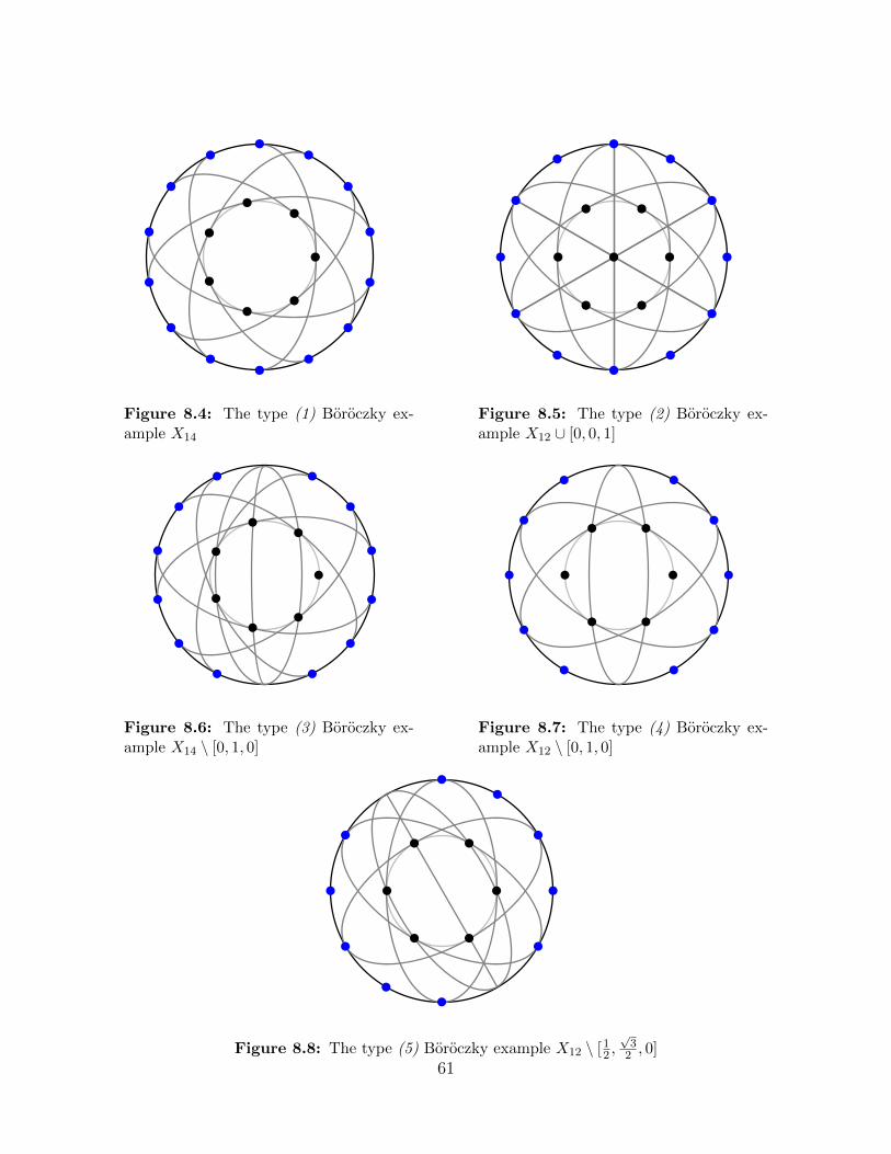
Figure 8.4: The type (1) Boroczky ex-ample X14

Figure 8.5: The type (2) Boroczky ex-ample X12 ∪ [0, 0, 1]

Figure 8.6: The type (3) Boroczky ex-ample X14 \ [0, 1, 0]

Figure 8.7: The type (4) Boroczky ex-ample X12 \ [0, 1, 0]

Figure 8.8: The type (5) Boroczky example X12 \ [12 ,√32 , 0]

61

8.3 The Sylvester Examples

The Sylvester examples are determined by the group law on the set Z(p)∗ of non-singular points of a homogeneous degree 3 polynomial p ∈ R[x, y, z]. For backgroundabout the group law on such curves, we refer the reader to Silverman and Tate [50].

We have already seen a classification of cubic curves up to projective equivalence inProposition 8.8. Since the group law on a cubic is preserved under projective transfor-mations, this classification can be used to produce a classification of the group Z(p)∗

in this case.

Proposition 8.11 ([50]). Let p ∈ R[x, y] be irreducible and homogeneous of degree 3.Recall that Proposition 8.8 classifies such the curves Z(p) up to projective equivalence.In the cases in the conclusion of this proposition, the group Z(p)∗ of non-singular pointsis isomorphic to:

1. (nodal case) R× Z/2Z;

2. (cuspidal case) R;

3. (acnodal case) R/Z;

4. (elliptic curve) R/Z if Z(p) has one connected component, or R/Z×Z/2Z if Z(p)has two connected components.

The Sylvester examples are either subgroups of these groups, or cosets of subgroups.

Definition 8.12. Let Z(p) be an irreducible cubic curve, and E be a subgroup of Z(p)∗

with |E| ≥ 3. Then we call the set E ⊂ PR2 a Sylvester example. In addition, ifx ∈ Z(p)∗ \ E and 3x ∈ E then we call the coset E ⊕ x a Sylvester example.

Since we require the Sylvester examples to have size |E| ≥ 3, these Sylvester exam-ples only exist in the acnodal or elliptic curve case, since in these cases the group Z(p)∗

has finite subgroups of size greater than two.

Proposition 8.13. Let E and E ⊕ x be Sylvester examples as per Definition 8.12.Recall that cP (2) denotes the number of ordinary lines spanned by P . Then

cE(2) =

{|E| − 1 if |E| ≡ 1, 2 (mod 3)|E| − 3 if |E| ≡ 0 (mod 3)

.

andcE⊕x(2) = |E| − 1.

Proof. Since a ⊕ b ⊕ c = 0 if and only if a, b, c ∈ Z(p)∗ are collinear, the number ofordinary lines in E⊕x is the number of elements a⊕x ∈ E⊕x satisfying a⊕x 6= 2a2x.To see this, observe that a⊕x,2a2x are collinear, 2a2x = (2a3x)⊕x ∈ E⊕x(here we use that 3x ∈ E), and the line joining them is tangent to Z(p) at a, so meets

62

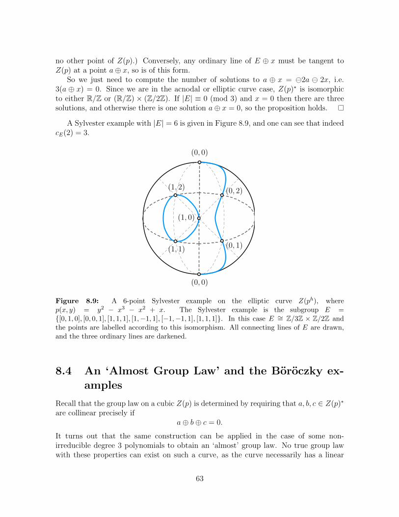
no other point of Z(p).) Conversely, any ordinary line of E ⊕ x must be tangent toZ(p) at a point a⊕ x, so is of this form.

So we just need to compute the number of solutions to a ⊕ x = 2a 2x, i.e.3(a ⊕ x) = 0. Since we are in the acnodal or elliptic curve case, Z(p)∗ is isomorphicto either R/Z or (R/Z) × (Z/2Z). If |E| ≡ 0 (mod 3) and x = 0 then there are threesolutions, and otherwise there is one solution a⊕ x = 0, so the proposition holds.

A Sylvester example with |E| = 6 is given in Figure 8.9, and one can see that indeedcE(2) = 3.

(1, 1)

(1, 2)

(1, 0)

(0, 0)

(0, 0)

(0, 1)

(0, 2)

Figure 8.9: A 6-point Sylvester example on the elliptic curve Z(ph), wherep(x, y) = y2 − x3 − x2 + x. The Sylvester example is the subgroup E ={[0, 1, 0], [0, 0, 1], [1, 1, 1], [1,−1, 1], [−1,−1, 1], [1, 1, 1]}. In this case E ∼= Z/3Z × Z/2Z andthe points are labelled according to this isomorphism. All connecting lines of E are drawn,and the three ordinary lines are darkened.

8.4 An ‘Almost Group Law’ and the Boroczky ex-

amples

Recall that the group law on a cubic Z(p) is determined by requiring that a, b, c ∈ Z(p)∗

are collinear precisely ifa⊕ b⊕ c = 0.

It turns out that the same construction can be applied in the case of some non-irreducible degree 3 polynomials to obtain an ‘almost’ group law. No true group lawwith these properties can exist on such a curve, as the curve necessarily has a linear

63

component and so any three points in this component must add to zero. The ‘almost’group law gives an operation which achieves this whenever only one of a, b, c lies in thelinear component.

Proposition 8.14 ([25, Proposition 7.3]). Let p = σl ∈ R[x, y, z], with σ and l ir-reducible of degree 2 and 1 respectively. Then there is an abelian group (G,⊕) withbijective maps

ψσ : G→ Z(σ)∗ and ψl : G→ Z(l)∗

so that ψσ(a), ψσ(b), and ψl(c) are collinear precisely if a ⊕ b ⊕ c = 0. Also, up toisomorphism we can classify G by

G ∼=

Z/2Z× R if |Z(σ) ∩ Z(l)| = 2R if |Z(σ) ∩ Z(l)| = 1R/Z if |Z(σ) ∩ Z(l)| = 0

As we will see later, the Boroczky examples are all subgroups and cosets of subgroupsarising from this almost group law.

Note that only in the case where the conic Z(σ) and the line Z(l) do not intersectcan G have large finite subgroups, and indeed the Boroczky examples lie on the unitcircle and the line at infinity which do not meet. For example Figure 8.10 we illustratethe Boroczky example X12 with points labelled according to the ‘almost’ group law.

1

2

3

4

5

0

0

12

3

4 5

Figure 8.10: The ‘almost’ group law on the Boroczky example X12. In this case G ∼= Z/6Zand we label the elements of X12 according to the bijections ψσ and ψl.

64

Chapter 9

Vanishing Polynomials

9.1 Melchior’s Inequality

As we have seen, one of the advantages of working in projective space is that the naturalduality between points and lines. In Section 8.1, we noted that this duality allowed usto translate incidence results into a dual version, replacing lines by points and pointsby lines. Melchior [37] noticed that looking at the dual P ∗ of P is a powerful tool forstudying the ordinary lines of P .

Definition 9.1. Let P ⊂ PR2 be a finite point set with |P | ≥ 2. The lines in P ∗

determine a (drawing of) a graph in PR2 by taking the vertices to be the points ofintersection of lines in P ∗ and the edges to be the line segments joining them. Wedenote the (multi)graph obtained in this fashion (and, abusing notation, the drawing)by ΓP and call it the projective dual graph of P .

Figure 9.1: Projective Dual Graphs

For example in Figure 9.1, the point set P = {[0, 0, 1], [1, 0, 0], [0, 1, 0]} has ΓPisomorphic to the multigraph on three vertices with each pair joined by two edges (inthis example the dual lines P ∗ are precisely the connecting lines of P .) Note that byconstruction the degree of each vertex is even, and for this example ΓP is a multigraph.We remark that since when studying point sets with few ordinary lines we assume thatnot all points are on a line, we will always have |P | ≥ 2. Melchior’s key observation isthat we can apply Euler’s formula to this graph.

65

Definition 9.2. Let G be a graph and Σ be a surface. An embedding (i.e. a drawing)of G in Σ is a 2-cell embedding if every face of the embedding is homeomorphic toan open disk.

For a thorough background on embedded graphs, the reader is advised to consultMohar and Thomassen [38].

Theorem 9.3 (Euler’s Formula). Let Σ be a surface. Then there exists a number χcalled the Euler characteristic of Σ such that for any 2-cell embedding of a graph Gin Σ,

V − E + F = χ,

where V,E, and F denote the number of vertices, edges and faces of the embedding,respectively.

When Σ is a plane we get the familiar result that planar graphs satisfy V −E+F = 2,since 2-cell embeddings into the plane are precisely planar drawings. We are concernedwith the case Σ = PR2. Note that not every embedding is a 2-cell embedding; forinstance the one-vertex graph with no edges has no 2-cell embedding into PR2, sinceevery embedding has exactly one face (PR2 minus a point) which is homeomorphic toa Mobius strip. However the drawing ΓP of the projective dual graph is always a 2-cellembedding when |P | ≥ 2.

To compute the Euler characteristic of PR2, consider the one-vertex graph with oneself loop. A 2-cell embedding is given by any line l ⊂ PR2 with a point p ∈ l; thenthe vertex in the drawing is p and the edge is l \ p. The embedding has only one face,PR2\l, which is indeed homeomorphic to an open disk. Thus V −E+F = 1−1+1 = 1,and the Euler number of PR2 is χ = 1. Melchior applied Euler’s formula to the dualgraph to count the number of ordinary lines in the following way.

Theorem 9.4 (Melchior’s Equality). Let P ⊂ PR2 be a finite set of points not all on aline. Let Nk denote the number of lines of P containing exactly k points and Ms denotethe number of faces of ΓP with exactly s edges. Then

N2 = 3 +∞∑k=4

(k − 3)Nk +∞∑s=4

(s− 3)Ms. (9.1)

Proof. Applying Euler’s formula to ΓP gives V − E + F = 1. We can count V,E, F inthe following ways:

V =∑∞

k=2Nk; 2E =∑∞

k=2 2kNk F =∑∞

s=3Ms.=∑∞

s=3 sMs;

These equalities follow since when we pass to the dual graph Nk is the number ofvertices of degree 2k, and we can count the number of edges either vertex-by-vertex(each is incident to 2 edges) or face-by-face (each is incident to 2 faces). We also use

66

the fact that M2 = 0, which follows from the assumption that P is not all on one line.Now we can substitute

0 = 3− 3F + 2E + E − 3V

= 3− 3∞∑s=3

Ms +∞∑s=3

sMs +∞∑k=2

kNk − 3∞∑k=2

Nk, and hence

N2 = 3 +∞∑k=4

(k − 3)Nk +∞∑s=4

(s− 3)Ms.

Since Ms and Nk are nonnegative, Melchior’s equality implies Corollary 7.4 (which,as we have noted, shows that P determines at least three ordinary lines.) However,Melchior’s inequality has much stronger consequences for point sets with few ordinarylines. Heuristically, if the number of ordinary lines N2 is small, then each of the positiveterms occurring on the right hand side of (9.1). That is, the dual graph ΓP containsvery few vertices of degree 2k for k ≥ 4 (or indeed for k = 2) and contains very fewfaces with four or more edges. So we expect that most faces are triangles and mostvertices have degree 6.

We now follow Green and Tao’s argument that makes this heuristic observationprecise, showing that the projective dual graph ΓP has a triangular grid like structure.

Definition 9.5. Let e = {u, v} be an edge of ΓP . We say e is good if both u and vhave degree six and the two faces adjacent to e are triangles. If e is not good we callit bad. We call e k-good if e is good and every path of length k from either u or vconsists entirely of good edges. If e is not k-good we call it k-bad.

e

u v

Figure 9.2: Locally, a goodedge looks like part of a trian-gular grid.

e

b

t edges

k − t− 1 edges

Figure 9.3: An example of a 9-good edge e, show-ing the existence of a path from e to a k-bad edgeb which changes direction only once.

A good edge looks like a component of a triangular grid (Figure 9.2), and the k-neighborhood of a k-good edge is a triangular grid (Figure 9.3 shows a 9-good edge e

67

and part of it’s k-neighborhood). Note that 0-good and 0-bad edges coincide with goodand bad edges. By the preceding discussion we expect the number of bad edges to bevery small for point sets determining few ordinary lines.

Theorem 9.6 ([25]). Let P ⊂ PR2 be a finite set of points not all on a line whichdetermines . |P | ordinary lines. Then the number of bad edges in ΓP is . |P | and foreach k ≥ 1 the number of k-bad edges in ΓP is . k2|P |.

Proof. If an edge e = {u, v} is bad then either u or v has degree 2k for k 6= 3, or elseone of the faces adjacent to e has four or more edges. Hence the number of bad edgesis at most the number of edges adjacent to such a face or such a vertex,

4N2 +∞∑k=4

2kNk +∞∑s=4

sMs.

Note that k ≤ 4(k − 3) if k ≥ 4, so by Melchior’s equality (9.1),

∞∑k=4

2kNk +∞∑s=4

sMs ≤ 8∞∑k=4

(k − 3)Nk + 4∞∑s=4

(s− 3)Ms ≤ 8N2.

So the number of bad edges is at most 12N2 . |P |.To bound the number of k-bad edges, we first consider edges that are k-bad but not

(k− 1)-bad. If e is such an edge, then there is a bad edge b at distance k from e, whilethe (k − 1)-neighborhood of e forms a triangular grid as in Figure 9.3. This triangulargrid structure means we can find a path from e to b that changes direction only once,and has length k. Furthermore, the vertex of b in the interior of this path has degree 6,since it is adjacent to a good edge. In this way we can associate to every k-bad edge e adistinct path from a bad edge b to e with the aforementioned properties. However sucha path is determined by the choice of b, the choice of direction to leave b, the numberof steps in that direction, the direction to change to, and which endpoint of e to arriveat; hence the number of such paths is at most

(# of bad edges)× 5× (k − 1)× 2 . k|P |.

Now the number of k-bad edges is the sum of the t-bad but not (t − 1)-bad edges fort = 0, . . . , k, which by the above is . k2|P |.

Thus for a fixed k, the number of k-bad edges is linear in the number of ordinarylines of P . If most points of P are contained in one line, the number of edges in ΓP canbe linear in |P |, but otherwise we expect the number of edges to be ∼ n2. So intuitivelythe previous lemma says that for fixed k most edges of ΓP are k-good when |P | is largeenough.

68

9.2 Polynomials Vanishing on P

We have seen that a point set P with few ordinary lines will have large regions oftriangular grid structure in its dual graph ΓP . In this section we see how that triangulargrid structure can be used to find especially low-degree vanishing polynomials.

Ultimately the reason that the triangular grid structure affords a particularly lowdegree vanishing polynomial is the following classical result of Chasles.

Proposition 9.7 (Chasles’ Theorem). Suppose that two sets of three lines in PR2

define nine distinct points of intersection and suppose p ∈ R[X, Y, Z] is a homogeneouspolynomial of degree at most 3. Then if eight of the intersection points are containedin Z(p), so is the ninth.

Figure 9.4: An illustration of Chasles theorem, showing two sets of three lines (light anddark) meeting at nine points, and a dashed cubic curve Z(p) which necessarily contains all ofthese points since it contains eight of them.

We will soon see that Proposition 9.7 can find a cubic polynomial that vanishes onall the points whose duals have a triangular grid structure, regardless of its size. Tomake this precise, we define what is meant by a triangular grid.1

Definition 9.8. Let P ⊂ PR2 be a finite point set and let I, J,K ⊂ Z be finitecontiguous subsets of Z. A triangular grid with dimensions I, J,K in P is a collectionof duals of points (p∗i )i∈I , (q∗j )j∈J , and (r∗k)k∈K , with all of pi, qj, rk in P , satisfying:

(1) whenever (i, j, k) ∈ I × J × K satisfy i + j + k = 0 the lines q∗i , p∗j , r∗k meet at a

point Pijk which is incident to no other line q∗i′ , p∗j′ , r

∗k′ in the grid;

(2) the intersection points Pijk arising from distinct triples are distinct;

(3) the points (pi)i∈I , (qj)j∈J , and (rk)k∈K are all distinct.

An example of a triangular grid is given is Figure 9.7. Definition 9.8 sets up a con-venient coordinate system on triangular grids. We will now translate Chasle’s theoreminto the language of triangular grids.

1Note that we have adopted a different definition than Green and Tao. As a result some of theforthcoming results are less general than those given in [25].

69

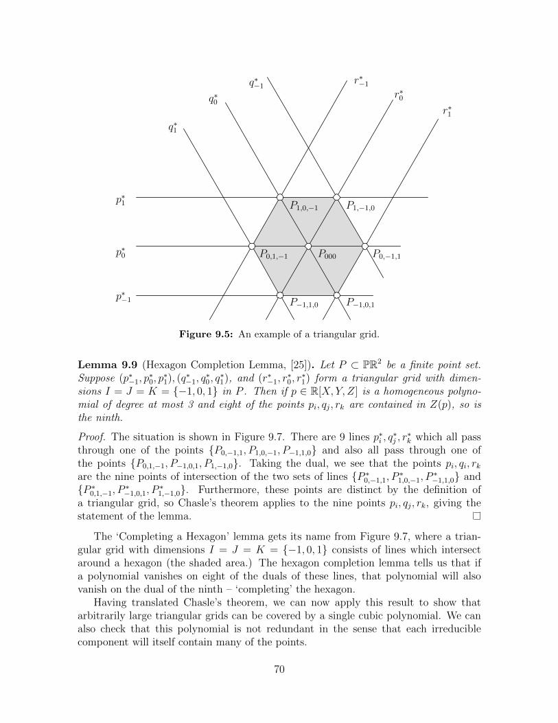
p∗−1

p∗0

p∗1

q∗−1q∗0

q∗1

r∗−1r∗0

r∗1

P000P0,1,−1 P0,−1,1

P1,0,−1 P1,−1,0

P−1,1,0 P−1,0,1

Figure 9.5: An example of a triangular grid.

Lemma 9.9 (Hexagon Completion Lemma, [25]). Let P ⊂ PR2 be a finite point set.Suppose (p∗−1, p

∗0, p∗1), (q

∗−1, q

∗0, q∗1), and (r∗−1, r

∗0, r∗1) form a triangular grid with dimen-

sions I = J = K = {−1, 0, 1} in P . Then if p ∈ R[X, Y, Z] is a homogeneous polyno-mial of degree at most 3 and eight of the points pi, qj, rk are contained in Z(p), so isthe ninth.

Proof. The situation is shown in Figure 9.7. There are 9 lines p∗i , q∗j , r∗k which all pass

through one of the points {P0,−1,1, P1,0,−1, P−1,1,0} and also all pass through one ofthe points {P0,1,−1, P−1,0,1, P1,−1,0}. Taking the dual, we see that the points pi, qi, rkare the nine points of intersection of the two sets of lines {P ∗0,−1,1, P ∗1,0,−1, P ∗−1,1,0} and{P ∗0,1,−1, P ∗−1,0,1, P ∗1,−1,0}. Furthermore, these points are distinct by the definition ofa triangular grid, so Chasle’s theorem applies to the nine points pi, qj, rk, giving thestatement of the lemma.

The ‘Completing a Hexagon’ lemma gets its name from Figure 9.7, where a trian-gular grid with dimensions I = J = K = {−1, 0, 1} consists of lines which intersectaround a hexagon (the shaded area.) The hexagon completion lemma tells us that ifa polynomial vanishes on eight of the duals of these lines, that polynomial will alsovanish on the dual of the ninth – ‘completing’ the hexagon.

Having translated Chasle’s theorem, we can now apply this result to show thatarbitrarily large triangular grids can be covered by a single cubic polynomial. We canalso check that this polynomial is not redundant in the sense that each irreduciblecomponent will itself contain many of the points.

70

(a) (b) (c)

(d) (e)

Figure 9.6: A pictorial view of the argument of Lemma 9.10. In (a) we see a section ofa triangular grid, and take a polynomial p vanishing on the 10 thick lines. We shade thosefaces of the grid enclosed by lines whose duals are contained in Z(p). In (b), applying thehexagon completion lemma to the darkened hexagon, we see that the dual of the red lineis contained in Z(p). Similarly in (c), (d), (e) we apply the hexagon completion lemma todifferent hexagons to find more lines with duals in Z(p).

Lemma 9.10. Let k ≥ 10 and m ≥ 3k be parameters and suppose that (p∗i )i∈I , (q∗j )j∈J ,and (r∗k)k∈K form a triangular grid in P with dimensions I = {−2k, . . . , 2k}, J ={−m, . . . , 1}, and K = {1, . . . ,m}. Then there is a homogeneous polynomial p ∈R[X, Y, Z] of degree at most 3 such that the points pi, qj, rk are all contained in Z(p)and for each irreducible factor h of p, Z(h) contains at least k of these points.

Proof. By the (proof of) Lemma 3.3, we can find a homogeneous polynomial p of degreeat most 3 which vanishes on the points

p−1, p0, p1, p2, q−3, q−2, q−1, r1, r2.

The aim is to repeatedly apply the hexagon completion lemma (Lemma 9.9) to concludethat p vanishes on the entire grid. Intuitively, we proceed as in Figure 9.6, using thehexagon completion lemma repeatedly to place the dual of every grid line inside Z(p).Formally we apply the hexagon completion lemma in several steps as follows:

(i) place r3 in Z(p) by applying the hexagon completion lemma to

(p∗0, p∗1, p∗2), (q

∗−n, q

∗−n+1, q

∗−n+2), (r

∗n−3, r

∗n−2, r

∗n−1)

71

(note that we can simply relabel the dimensions to {−1, 0, 1} to apply the lemma)

(ii) for n = 4, 5, . . . ,m, place q−n and rn in Z(p) by applying the hexagon completionlemma to

(p∗0, p∗1, p∗2), (q

∗−n, q

∗−n+1, q

∗−n+2), (r

∗n−3, r

∗n−2, r

∗n−1)

and then to(p∗−1, p

∗0, p∗1), (q

∗−n, q

∗−n+1, q

∗−n+2), (r

∗n−2, r

∗n−1, r

∗n)

(iii) for n = 3, 4, . . . , 2k, place pn in Z(p) by applying the hexagon completion lemmato

(p∗n−2, p∗n−1, p

∗n), (q∗−n−2, q

∗−n−1, q

∗−n), (r∗1, r

∗2, r∗3)

(note the assumption m ≥ 3k ensures this step is well-defined.)

(iv) for n = 2, 3, . . . , 2k, place p−n in Z(p) by applying the hexagon completion lemmato

(p∗−n, p∗−n+1, p

∗−n+2), (q

∗−3, q

∗−2, q

∗−1), (r

∗n, r∗n+1, r

∗n+2)

To investigate the number of points lying on each irreducible component, consider triplesof points (pi, qj, rk) with i + j + k = 0 whose duals lie in the grid. Observe that thereare at most three triples for which the line P ∗ijk is contained in Z(p), since the Pijk aredistinct (by definition of a triangular grid) and p has degree 3 so by Lemma 3.8, Z(p)contains at most 3 lines. Now any other triple (pi, qj, rk) contains at least one pointin each irreducible component of Z(p), since they are distinct points of intersection ofthe line P ∗ijk with Z(p) and by Lemma 3.5 each irreducible component contains only asmany points as its degree.

Hence we look at the k + 3 triples

(pn, q1−2n, rn+1)

for n = 1, 2, . . . , k + 3. Note that k + 3 ≤ 2k, 1 − 2(k + 3) = −2k − 5 ≥ −3k ≥ −mand (k + 3) + 1 ≤ 3k ≤ m. Thus the duals of the points in these triples are in thegrid. Furthermore, the points appear in at most one triple and are distinct by thedefinition of a triangular grid. By the previous paragraph, except for at most 3 of thesetriples, each contains at least one point in each irreducible component. Hence by thedistinctness of points across triples, each irreducible component contains at least k ofthe points pi, qj, rk.

Lemma 9.10 states the remarkable fact that the dual of an arbitrarily large triangulargrid (with dimensions of the specified form) can be covered by a single cubic curve Z(p).We now see how this is applicable to the triangular grid-like structure that arises fromk-good edges.

72

Corollary 9.11. Let P ⊂ PR2 be a finite point set which cannot be covered by 4kconcurrent lines, and let k ≥ 1 and m ≥ 3k be parameters. Suppose that p∗0 ∈ P ∗

contains a segment s of m consecutive k-good edges of ΓP , as well as at least 4k otheredges. Denote by P0,−1,1, P0,−2,2, . . . , P0,−m,m the ordered vertices in the segment s. Alsolet Ps be the set of points q ∈ P \ {p} such that q∗ is incident to one of the verticesP0,−j,j in s. Then there is a polynomial p of degree at most 3 such that Ps ∈ Z(p), andeach irreducible factor h of p satisfies |Z(h) ∩ P | ≥ k.

p∗−2

p∗−1

p∗0

p∗1

p∗2

r∗5 r∗4 r∗3 r∗2 r∗1

q∗−5 q∗−4 q∗−3 q∗−2 q∗−1

s

Figure 9.7: Labelling the 2-neighborhood of a segment s consisting of 4 consecutive 2-goodedges (k = 1,m = 4)

Proof. The proof amounts to observing that the 2k-neighborhood of the 2k-good edgesforms a triangular grid,

(p∗−2k, . . . , p∗0, . . . , p

∗2k), (q

∗−m, . . . , q

∗−1), (r

∗1, . . . , r

∗m)

with dimensions {−k, . . . , 0, . . . , k}, {−m, . . . ,−1}, {1, . . . ,m}. Formally, this can bechecked by defining the pi, qj, rk inductively using the definition of a good edge andthe construction of the projective dual graph ΓP . Labelling the lines of the grid as inFigure 9.7, the vertices Pijk exist by construction and are incident to no other line sincethey have degree 6. Since P cannot be covered by 4k concurrent lines, and since p∗0contains at least m extra edges outside the contiguous k-good ones, the collection oflines p∗i , q

∗j , r∗k are all distinct. Lastly, since these lines are distinct and each vertex has

degree 6 the intersection points Pijk must all be distinct also.Having checked that this 2k-neighborhood is indeed a triangular grid, the result

follows from Lemma 9.10.

We have already seen that in a point set P with few ordinary lines, we expect mostedges to be k-good (for fixed k). Corollary 9.11 tells us that consecutive segments ofk-good edges are intersected by lines p∗ whose duals p all lie within a single low-degreepolynomial. The next step is to look at all edges along a given line p∗0, and applyLemma 9.11 to clusters of k-good edges.

73

Lemma 9.12. Let k ≥ 10 be a parameter. Let P ⊂ PR2 be a finite point set, whichspans at most |P | ordinary lines and which cannot be covered by 4k concurrent lines.Then for every q ∈ P , there is a polynomial

p =

Nq∏i=1

pi

Mq∏i=1

li = p1p2 . . . pNq l1l2 · · · lMq

and points sets Li ⊂ P for i = 1, . . . ,Mq, and Pi ⊂ P for i = 1, . . . , Nq such thatP ⊂ Z(p), Li ⊂ Z(li), Pi ⊂ Z(pi) and

(i) 1 ≤ deg(pi) ≤ 3 for all i = 1, . . . , Nq and deg(li) = 1 (the li are lines);

(ii) q ∈ Z(li) for i = 1, . . . ,Mq and q ∈ Z(pi) for i = 1, . . . , Nq;

(iii) each irreducible factor h of pi satisfies |Z(h) ∩ P | ≥ k;

(iv) the decomposition

P = {q} ∪ L1 ∪ · · ·LMq ∪ P1 ∪ · · · ∪ PNq

is a partition of P and the points in Pi can be partitioned into pairs (a, b) suchthat q, a, b are collinear and the line through these points meets no other point ofP .

Furthermore, the number of factors Nq +Mq can be bounded in aggregate as∑q∈P

(Nq +Mq) . k3|P |. (9.2)

Proof. Consider the line q∗. Removing the 2k-bad edges from this line leaves somenumber of segments consisting of only 2k-good edges, which we denote s1, . . . , st.Let|si| denote the number of edges in the segment si and without loss of generality weassume |s1| ≥ · · · ≥ |st|. Also let |q∗| denote the number of edges on q∗.

Construct the polynomial p according to one of the following cases:

Case 1: |q∗| ≤ 14k.

Let v1, . . . , vMq be the vertices on q∗. For each i = 1, . . . ,Mq we let li be thelinear polynomial with Z(li) = v∗i , and take p = l1 · · · lMq .

Case 2: |q∗| > 14k, and |q∗| − |s1| ≤ 4k (s1 contains all but ≤ 4k edges of q∗.)

Let s0 be the segment consisting of the first |q∗|−4k edges in s1, and v1 . . . , vMq

be the remaining vertices in q∗ but not in s0. As in Case 1, choose li withZ(li) = v∗i . Apply Corollary 9.11 to the segment s0 to construct a polynomialp1 of degree at most 3 vanishing on Ps0 . Let Nq = 1 and p = l1 · · · lMqp1, anddefine P1 = Ps0 .

74

Case 3: |q∗| > 14k, and |s1| < |q∗| − 4k (every segment contains < |q∗| − 4kedges.)

Let s′1, . . . , s′Nq

be those segments of the si containing at least 10k edges, andlet v1 . . . , vMq be the remaining vertices in q∗ not contained in any of the s′i.As before we choose li with Z(li) = v∗i , and apply Corollary 9.11 to eachsegment s′i to construct a polynomial pi of degree at most 3 vanishing on Ps′i .This gives the polynomial p = l1 · · · lMqp1 · · · pNq , and we define Pi = Ps′i .

It remains to define the sets Li, which we do by letting in each case Li be the set ofq ∈ P such that q∗ is incident to vi. We now check the statements (i)–(iv).

(i) By construction each li is linear and each pi is nonzero of degree at most 3.

(ii) Since q∗ is incident to vi, q ∈ Z(li) for i = 1, . . . ,Mq. By construction of the pifrom Corollary 9.11, q ∈ Z(pi) for each i = 1, . . . , Nq.

(iii) Since each p was constructed by applying Corollary 9.11, each irreducible factorh of pi satisfies |Z(h) ∩ P | ≥ k.

(iv) If q0 ∈ P with q0 6= q then q∗0 meets q∗ in precisely one point. If this point issome vi then p ∈ Li, and if this point is in a segment s then p ∈ Ps = Pj for somej = 1, . . . , Nq. Since the segments and vertices vi are in each case disjoint andexhaust the points on q∗, their union is a partition.

To see that points can be paired up, to each point a ∈ Pi we can associate thepoint b ∈ Pi where q∗, a∗, b∗ meet (it exists since a∗ meets q∗ at an endpoint of agood edge, where three lines meet.) In this way the set can be partitioned intopairs and moreover since the vertex where q∗, a∗, b∗ meet has degree exactly six,no other line c∗ is incident to this point, so no other point is on the line throughq, a, b.

Lastly, we wish to bound the sizes Nq + Mq of the polynomials. Let Bq denote thenumber of 2k-bad edges on q∗. Hence by Lemma 9.6,

∑q∈P Bq . k2|P |. Then

Mq ≤ max{14k, 4k, (10k + 1)Bq} . kBq and Nq ≤ Bq.

Therefore Nq +Mq . kBq, and hence by Theorem 9.6,∑q∈P

(Nq +Mq) . k3|P |

To understand the previous result, note that a simple application is the following,which is proved separately in Green and Tao as [25, Proposition 5.1] and does not usemost of the special structure of the constructed polynomial.

Corollary 9.13. Let P ⊂ PR2 be a finite point set, which spans at most |P | ordinarylines. Then there is a polynomial p of bounded degree, each irreducible factor of whichhas degree at most 3, such that P ⊂ Z(p).

75

Proof. Let k = 10 (we could just as well take any other fixed k ≥ 10). If P can becovered by 4k concurrent lines then we simply take p such that Z(p) is the union ofthese lines. Otherwise, we obtain the polynomial p by applying Lemma 9.12 for theq ∈ P which minimises Nq +Mq, which must satisfy

Nq +Mq ≤1

|P |∑q∈P

(Nq +Mq) . k3.

Since k3 is constant and the degree of p is at most 3(Nq +Mq), the corollary holds.

We take a moment to remark on the strength of this result: an arbitrarily largepoint set can be placed inside the zero set of a constant degree polynomial, providedthat the point set spans few ordinary lines!

9.3 Reducing to a single cubic

Lemma 9.12 shows that we can place P inside a polynomial of low degree with onlylinear, quadratic and cubic factors. The next step will be to show that in fact, all butone of those factors is linear.

Theorem 9.14. Let P ⊂ PR2 be a finite point set which spans at most |P | ordinarylines. Then there is a polynomial p and a partition P = P ′ ∪ P ′′ such that P ′ ⊂ Z(p)and either

(1) p = l1 · · · lN where the li are linear, N . 1 and |P ′′| . 1;

(2) p is irreducible of degree 3, and |P ′′| . 1;

(3) p is irreducible of degree 2, P ′ = Z(y1) ∩ P , P ′′ = Z(l1 · · · lN) ∩ P where N . 1and the li are linear, ||P ′| − |P ′′|| . 1 and P ′′ spans . |P | ordinary lines.

Proof. We split into cases:

Case 1: P can be covered by . 1 concurrent lines.

In this case we simply take the li to be the defining polynomials of these lines,and (1) holds.

If we are not in Case 1, then apply Lemma 9.13 to find a polynomial y = y1 · · · ym suchthat

P ⊂ Z(y) = Z(y1) ∪ . . . ∪ Z(ym)

where m . 1 and each yi is irreducible of degree at most 3.

Case 2: P cannot be covered by . 1 concurrent lines, and there is no yi ofdegree 2 or 3 satisfying |Z(yi) ∩ P | & 1.

In this case (1) holds if we take the li to be those factors yj of degree one, sothat N ≤ m . 1. Since each non-linear factor contains . 1 points of P , thereare . 1 points of P not lying on one of the lines Z(li).

76

If we are not in Case 2 then there is some factor, without loss of generality y1, whichhas degree 2 or 3 and satisfies

|Z(y1) ∩ P | & 1. (9.3)

We denote by P0 those points of P ∩ Z(y1) which are not contained in Z(yi) for anyi 6= 1. By Bezout’s Theorem (we state Theorem 4.3 in the plane, but it extends to theprojective plane) each yi, i 6= 1, satisfies |Z(y1) ∩ Z(yi)| ≤ 9. Hence

|P0| ≥ |P | − 9m ≥ |P |/2. (9.4)

Since we are not in Case 1, P cannot be covered by . 1 concurrent lines, so for anyq ∈ P we can apply Lemma 9.12 with k = 10m to obtain a polynomial

p = l1 . . . lMp1 . . . pN

with P ⊂ Z(p) and satisfying Lemma 9.12(i)–(iv). By the pigeonhole principle, we canchoose a point q ∈ P ′ such that cq is at most the average value for q ∈ P ′. By (9.2) wethus fix q so that

Nq +Mq ≤1

|P0|∑r∈P ′

(Nr +Mr) ≤1

|P0|∑r∈P

(Nr +Mr) .1

|P0||P |. (9.5)

Recall that from Lemma 9.12(ii), each irreducible component h of pi satisfies |Z(h) ∩P | ≥ 10m. If pi does not have yj as an irreducible component, then |Z(h)∩Z(yj)| ≤ 9by Bezout’s Theorem, so

|Z(h) ∩ P | ≤ |Z(h) ∩ Z(y)| ≤ 9m.

Hence the irreducible components of pi are each equal to yj for some j = 1, . . . ,m. ByLemma 9.12(i), q ∈ Z(pi). However q ∈ P0 so q ∈ Z(y1) and q is not contained in anyother Z(yi). Hence every pi contains y1 as a factor. We now split into cases dependingon the degree of y1.

Case 3: P cannot be covered by . 1 concurrent lines, and y1 has degree 3.

Every pi contains y1 as a factor, so since the pi are distinct we must have Nq = 1and p1 = y1. Let P ′ = P ∩ Z(p1) and P ′′ = P \ P ′. Since q ∈ Z(li) for each i,li is not identical to any yi, so

|Li| ≤ |Z(li) ∩ P | ≤ |Z(li) ∩ Z(y)| ≤ 3m

by Bezout’s theorem. Hence |P ′′| ≤ ∑Mq

i=1 |Li| ≤ 3mMq . |P ||P0| . 1 and so

statement (2) holds.

Case 4: P cannot be covered by . 1 concurrent lines, and y1 has degree 2.

Every pi contains y1 as a factor. To see that no pi can be of degree 2, recallfrom Lemma 9.12(iv) that there is a pair of points a, b ∈ Z(pi) \ {q} such that

77

q, a, b ∈ Z(pi) are collinear, which cannot happen if pi has degree 2. Hence, fori = 1, . . . , N , pi = y1vi where vi is linear and vi = yj for some j = 1, . . . ,m.

Recall that Lemma 9.12(iv) partitions Pi into pairs, and observe that onemember of each pair must lie on Z(y1) and one on Z(vi) (since any line throughZ(p) meeting three points must intersect Z(y1) twice and Z(vi) once.) Define

P ′ = P ∩ Z(y1) and P ′′ = P ∩ Z(l1 · · · lMv1 · · · vN).

Then |P ′| + |P ′′| = |P | and |P ′′|, |P ′| ≥ ∑Mi=1 |Pi|/2. By Bezout’s theorem as

in Case 3, |Li| ≤ 3m and hence∑M

i=1 |Pi| ≥ |P | − C where C . 1. Thus||P ′| − |P ′′|| . 1.

It remains to check how many ordinary lines are determined by P ′′. An ordinaryline in this set is either:

(a) ordinary in P ;

(b) contains a point of P ′ \ P0 and exactly two points of P ′′; or

(c) contains a point of P0 and exactly two points of P ′′.

There are at most |P | ordinary lines of the type (a) by assumption. Thereare at most |P ′′||P ′ \ P0| ≤ 9m|P ′′| . |P | of type (b) since |P ′ \ P0| ≤ 9m(by (9.4)). Lastly consider an ordinary line of the type (c), passing through apoint a ∈ P ′. Applying Lemma 9.12 as we have already done, we get anotherpolynomial p = p′1 · · · p′Na

l′1 · · · l′Maand partition L′i,M

′i . As we have already

seen, p′i = y1vi for a linear factor vi = yj. By Lemma 9.12(iv), any line througha and a point of Pi is incident to exactly one point of P ′′, so such a line cannotbe ordinary in P ′′. Hence an ordinary of type (c) which passes through a mustbe one of the Z(l′i), and so there are at most Ma such lines. Summing over alla ∈ P0, therefore by (9.2) there are . |P |+∑a∈P0

Ma . |P | ordinary lines forP ′′.

Therefore statement (2) holds.

In each case one of the statements (1)–(3) holds, so we are done.

Theorem 9.14 already classifies point sets with few ordinary lines to an extent, andit has been obtained using only polynomial and combinatorial methods. In Chapter 10we give Green and Tao’s introduction of ideas from arithmetic combinatorics to con-siderably simplify this classification.

78

Chapter 10

The Green-Tao proof

We have already seen in Section 6.3 how results in combinatorial geometry can be usedto prove results in arithmetic combinatorics, by considering special point sets. In thischapter, we show that the inverse dynamic can hold: arithmetic combinatorics canprove results in combinatorial geometry. This will finally resolve Theorem 7.6 by givinga simple classification of point sets spanning at most |P | ordinary lines.

10.1 Background Material

To begin, we present without proof the relevant results from arithmetic combinatorics.Some of the proofs can be found in [25, Appendix A], though as before the book [57] isan excellent reference.

We have already seen the Boroczky and Sylvester examples which lie on degree 3algebraic curves, and we have seen that the relationship of collinearity gives rise to agroup (or ‘almost’ group) structure on points of these curves. The following lemmarelates point sets with few ordinary lines with the group structure.

Lemma 10.1 ([25, Proposition A.4]). Let (G,+) be an abelian group and A,B subsetsof G, with ||A| − |B|| . 1. If there are . |A| pairs (a, a′) ∈ A2 for which a + a′ 6∈ B,then there is a subgroup H of G and a coset x+H such that

|A4(H + x)|, |B4(H + 2x)| . 1.

Roughly speaking, Lemma 10.1 says that unless A is a coset of a subgroup of G, thesum A+A in G will be larger than A. The reader should contrast this with Freiman’stheorem, which similarly says there is additive structure in A ⊂ Z whenever A + A issmall.

We do not give the proof of the following result of Green and Tao, which rules outexamples of point sets with few ordinary lines that lie on a small constant number oflines.

79

Lemma 10.2 ([25, Proposition 6.1]). Let P ⊂ PR2 be a finite point set which spans. |P | ordinary lines, and suppose that P is contained in the union of . 1 lines. Thenif |P | & 1, all except . 1 of the points of P lie on a single line.

This result considerably simplifies the conclusion of Theorem 9.14, reducing in eachcase to just one line.

Theorem 10.3. Let P ⊂ PR2 be a finite point set which spans at most |P | ordinarylines, and suppose |P | & 1. Then there is a subset P0 ⊂ P with |P \ P0| . 1 and ahomogeneous polynomial p ∈ R[x, y, z], satisfying P0 ⊂ Z(p), of one of the followingforms:

(1) p is irreducible of degree 1;

(2) p is irreducible of degree 3;

(3) p = σl where σ, l are irreducible and have degrees 2 and 1 respectively, and

||Z(σ) ∩ P0| − |Z(l) ∩ P0|| . 1.

That is, P ′ lies on either a line, an irreducible cubic curve, or on the union of anirreducible conic curve and a line.

Proof. We apply Theorem 9.14 to P . In cases (1) and (3), we apply Lemma 10.2 tothe points lying on Z(l1 · · · lN) to conclude all but . 1 of these points lie on a singleline l. In case (3), we then define P0 = Z(p) ∩ P and can check that Z(σ) ∩ P0 = P ′

and ||Z(l) ∩ P0| − |P ′′|| . 1, so the result holds.

Theorem 10.3 classifies point sets spanning few ordinary lines to a sufficient extentto solve the Dirac-Motzkin conjecture for large |P |. In the next section we give theresolution of the problem by applying Theorem 10.3.

10.2 The Green–Tao proof

The results of Section 10.1 together show that the Boroczky examples are the pointsets determining fewest ordinary lines.

Theorem 10.4 ([25, Theorem 2.4]). Let P ⊂ PR2 be a finite non-collinear point setwhich spans at most |P | − C ordinary lines, where C is an absolute constant. Then Pis projectively equivalent to one of the Boroczky examples (c.f. Proposition 8.10.)

Proof. Since P spans at most |P | ordinary lines, by Theorem 10.3 there is a subsetP ′ ⊂ P with |P \ P ′| . 1 and a polynomial p with P ′ ⊂ Z(p) and satisfying one of(i)–(iii).

We redefine P ′ = P ′ ∩ Z(p)∗, which removes at most two singular points fromP ′. Observe that the set P ′ itself spans . |P | ordinary lines, since P spans at most

80

|P |, and the number of connecting lines of P ′ containing a point of P \ P ′ is at most|P ||P \ P ′| . |P |.

We will now examine each possibility in Theorem 10.3.

Case (1). If p is irreducible of degree 1, then since the points are non-collinear we canchoose a ∈ P \ P ′. At most . 1 of the lines joining a to a point of P ′ arenot ordinary, since such lines must contain another point of P \ P ′. HenceP determines at least |P | − C1 ordinary lines for some absolute constantC1 . 1.

Case (2). If p is irreducible of degree 3, consider the group Z(p)∗. A pair of pointsa, b ∈ P ′ determines an ordinary line of P ′ if and only if the point a b isnot in P ′. Hence for all but . |P | pairs a, b ∈ P ′, ab ∈ P ′ or equivalentlya⊕ b ∈ P ′.Hence, applying Lemma 10.1 with A = P ′, B = P ′, there is a subgroup Eof Z(p)∗ and a coset E ⊕ x such that

|P ′4(E ⊕ x)|, | P ′4(E ⊕ 2x)| . 1.

So, P ′ is almost entirely a coset of a subgroup of Z(p)∗. Additionally, since|P ′4(E⊕2x)| = |P ′4(E2x)|, we have |(E⊕2x)4(E⊕x)| . 1. Howeverdistinct cosets do not overlap, so if |P | is large enough (this is ensured bytaking the absolute constant C large enough) this implies 3x ∈ E.

This shows that E ⊕ x is a Sylvester example, and P ′′ = P ∩ (E ⊕ x) isalmost all of P , since

|P \ P ′′| = |P \ (E ⊕ x)| ≤ |P \ P ′|+ |P ′4(E ⊕ x)| . 1.

Now we wish to compute the number of ordinary lines spanned by P . Recallfrom Proposition 8.13 that E ⊕ x spans at least |E| − 3 ordinary lines, andeach point of E⊕x lies on at most two ordinary lines. Hence after removingthe points (E⊕x) \P ′′ from E⊕x, at least |E| −C ′2 ordinary lines remain,where C ′2 . 1. In addition, a point not lying in Z(p) lies on at most 3tangent lines to Z(p), so after adding the points of P \P ′′ at least |E| −C2

ordinary lines remain, where C2 . 1. Hence by taking C large enough, Pspans at least |P | − C ordinary lines in this case.

Case (3). If p = σl where σ, l are irreducible and have degrees 2 and 1 respectively,then consider the group G from Proposition 8.14 which imbues Z(p)∗ withan almost group structure. Write Pσ = P ′ ∩ Z(σ)∗ and Pl = P ′ ∩ Z(l)∗.Recalling the maps from G into Z(σ)∗ and Z(l)∗, we consider the preimages

Σ = ψ−1σ (Pσ) and L = ψ−1l (Pl).

81

As in Case (i), for all but . |Σ| pairs a, b ∈ Σ, a ⊕ b ∈ L. Furthermore||Σ| − |L|| . 1 by Theorem 10.3(ii), since |Σ| = |Pσ| and |L| = |Pl|.Hence as before we can apply Lemma 10.1 with A = Pσ, B = L, to find asubgroup H of G and a coset H ⊕ x such that

|Σ4(H ⊕ x)|, |L4(H 2x)| . 1.

For |P | large enough we must have |Z(σ)∩Z(l)| = 0, since otherwise G ∼= Ror G ∼= R × Z/2Z and so G has no finite subgroups with more than twoelements. Hence G ∼= R/Z, and H = {i/m | i = {0, 1, . . . ,m− 1}}.We do not give the details (see [25, Proposition 7.3, Lemma 7.4, Proposition8.2]) but with the explicit form of the bijections ψσ, ψl one can check thatψσ(H ⊕ x) ∪ ψl(H 2x) is projectively equivalent to the set X2m, andadditionally that any set P with |P4X2m| . 1 and spanning at most |P | −C3 ordinary lines is a Boroczky example, where C3 . 1 is an absoluteconstant. Ensuring C is large enough, we conclude that P is a Boroczkyexample.

We see that for large enough C, only in case (3) can P span at most |P |−C ordinarylines, and in this case P must be a Boroczky example.

Theorem 10.4 is a strong classification of point sets determining few ordinary lines.From this, Green and Tao’s bound for the Dirac-Motzkin conjecture for large |P | follows.

Theorem 7.6 ([25, Theorem 2.2]). Let P ⊂ PR2 be a finite non-collinear point set,with |P | & 1, then

cP (2) ≥

12|P | if |P | ≡ 0, 2 (mod 4)

34(|P | − 1) if |P | ≡ 1 (mod 4)

34(|P | − 3) if |P | ≡ 3 (mod 4)

.

Proof. Applying Theorem 10.4, P is projectively equivalent to a Boroczky example.Since the number of ordinary lines is preserved under such transformations, the boundson cP (2) hold by Proposition 8.10.

Theorem 7.6 solves Dirac and Motzkin’s Conjecture 7.5 for large |P |. The method ofits proof, and in particular the use of additive combinatorics, suggest that this methodcan not be extended to cover the small |P | case. We note that the implicit constantin Theorem 7.6 can be computed, and is sufficiently large that checking the remainingexamples is impractical.

82

Chapter 11

Isosceles Triangles

Recall that Erdos’ distinct distances problem asks for a lower bound on the number d(P )of distinct distances determined by the finite point set P . A closely related problem isto bound the number of distances da(P ) = |{||a − b|| | b ∈ P}| around a single pointa ∈ P . Denote

dp(P ) = maxp∈P

(dp(P )).

Finding a tight lower bound for dp(P ) is another open problem. The current best knownbound is dp(P ) & |P |0.8641... due to Katz and Tardos [32]. In fact, until the result ofGuth and Katz, every known lower bound for d(P ) proceeded by bounding dp(P ) andusing the trivial observation that dp(P ) ≤ d(P ).

One can think of these distance problems as concerning properties of two-pointsubsets of P . From this point of view, it is natural to study properties of n-pointsubsets of P . A 3-point subset of P determines a triangle, and a natural subject tostudy has been the number of isosceles triangles,

i(P ) = {(a, b, c) | a, b, c ∈ P, |a− b| = |b− c| 6= 0}.Note that degenerate isosceles triangles are included in the count, and each isoscelestriangle is counted more than once. A random point set will almost certainly containno isosceles triangles, whereas a point set P consisting of a regular n-gon and its centrewill determine & |P |2 isosceles triangles.

Intuitively, the number of isosceles triangles and the number of distinct distancesshould be related, because isosceles triangles arise from repeated distances from a singlepoint. We can make this intuition precise.

Proposition 11.1. Let P ⊂ R2 be a finite planar point set, then

|i(P )|dp(P ) & |P |3.Proof. Consider a single point a ∈ P . Partition P = P1 ∪ · · · ∪ Pda(P ) such that all thepoints in Pi are at the same distance from a. Then

ia(P ) = |{(a, b, c) | b, c ∈ P, ||a− b|| = ||b− c||}| =da(P )∑i=1

(|Pi|2

). (11.1)

83

Since |P | = ∑da(P )i=1 |Pi| is fixed, the sum (11.1) is minimised when |Pi| = |P |/da(P ), so

ia(P ) ≥ |P |2/da(P ). Finally,

|i(P )| =∑a∈P

ia(P ) ≥∑a∈P

|P |2/da(P ) ≥ |P |3/dp(P ).

Proposition 11.1 suggests that one way to attack the distinct distances problem is byfinding an upper bound on the number of isosceles triangles. The following propositionshows that this approach cannot improve on the Guth-Katz result (Theorem 1.5). Thefollowing computation first appears in Erdos and Purdy [20].

Proposition 11.2 ([20]). Let P = {−2n, . . . , 2n}2 be a (4n+ 1)× (4n+ 1) grid in theplane. Then |i(P )| & |P |2 log |P |.

Proof. First consider the grid P0 = {−n, . . . , n}2. Denote i0(P0) = {(0, a, b) ∈ i(P0)}.Let (0, a, b) ∈ i0(P0) be an isosceles triangle and let a = (ax, ay) and b = (bx, by).Then a2x + a2y = b2x + b2y and a2x + a2y ≤ 2n2. Denote by r2(k) the number of pairs(x, y) ∈ Z2 satisfying x2 + y2 = k. Each pair (x, y) satisfying x2 + y2 ≤ n2 lies in P0, so

|i0(P0)| ≥∑n2

k=0 r2(k)2. Sums of this form have been well studied [28, 44, 4], and canbe bounded as follows

|i0(P0)| ≥n2∑k=0

r2(k)2 & n2 log n. (11.2)

Now consider the grid P . Note that P0 ⊂ P and that for each a ∈ P0, a + P0 ⊂ P .Since a + P0 is a translate of P0, by (11.2) there are & n2 log n isosceles triangles(a, a+ b, a+ c) ∈ i(P ) with b, c in P0. Therefore

|i(P )| ≥ |P0|n2 log n & |P |2 log |P |.

By Proposition 11.2, one cannot hope to find a better upper bound than |i(P )| .|P |2 log |P | for general point sets. It is conjectured that this upper bound holds.

Conjecture 11.3. If P is a finite point set in the plane, then |i(P )| . |P |2 log |P |.

In the next section, we give a proof of a weaker bound than Conjecture 11.3 by thepolynomial method.

11.1 An upper bound by the polynomial method

We begin by transforming the isosceles triangle problem to an incidence problem in themanner of Chapter 2. Recall that G is the group of orientation-preserving rigid motionsof the plane (the translations and rotations). We first define all of our terms; the readermay wish to refer to Chapter 2 to see the correspondence with Elekes’ reduction.

84

Definition 11.4. Define a map F : i(P ) → G by letting F (a, b, c) be the uniquerotation g around a satisfying gb = c. Define

H=k(P ) = {g ∈ G | g is a rotation about a point a ∈ P and |gP ∩ P | = k}

and H≥k = ∪∞j=kH=j(P ). Recall that we decomposed G = Grot ∪ Gtrans into rotationsand translations. Let H trans

≥k (P ) = H≥k(P ) ∩Gtrans and Hrot≥k (P ) = H≥k(P ) ∩Grot.

By analogy with Lemma 2.3, we get the following.

Lemma 11.5. If g ∈ H=k(P ) then |F−1(g)| = k − 1.

Proof. Let gP ∩ P = {a, p1, . . . , pk−1}. Then pi = gqi for some qi ∈ P , and hence(a, qi, pi) ∈ F−1(g). Conversely, if (a, b, c) ∈ F−1(g) then gb = c so c ∈ gP ∩ P . Hencec = pi for some i.

If g ∈ G is not a rotation about a point a ∈ P then F−1(g) = ∅, so

|i(P )| =|P |∑k=2

(k − 1)|H=k(P )| =|P |∑k=2

|H≥k(P )|. (11.3)

To interpret bounding |H≥k(P )| as an incidence problem, we get the following analogueof Lemma 2.4. Recall the definition Sp,q = {g ∈ G | gp = q}.

Lemma 11.6. Suppose 2 ≤ k ≤ |P | and let L = {Sp,q | p, q ∈ P and p 6= q} andR = {Sa,a | a ∈ P}. Then |H≥k(P )| is the number of elements g ∈ G contained in aset L0 ∈ R and contained in at least k − 1 distinct sets L1, . . . , Lk−1 ∈ L.

As in Lemma 2.9, there cannot be too many such points that are translations.

Lemma 11.7. |H trans≥k (P )| . |P |2/k

We omit the proofs of Lemmas 11.7 and 11.6, as they are almost the same asthe proofs of the quotes similar results. Recall the parameterisation ρ : Grot → R3

introduced by Guth and Katz in (2.4). From Lemma 2.10, the sets Lp,q = ρ(Sp,q ∩Grot)are lines in R3. By Lemma 11.6, |Hrot

≥k (P )| is precisely the number of incidences betweenat least k − 1 lines Lp,q with p 6= q and a line La,a, where all of p, q, a are in P . Thisreduces the isosceles triangle problem to an incidence problem about lines in R3, asfollows:

Definition 11.8. Define L = {Lp,q | p, q ∈ P and p 6= q} and R = {La,a | a ∈ P}.

As in Section 2.2, the sets of lines L and R have important properties.

Proposition 11.9.

(1) |L| = |P |2 − |P | and |R| = |P |;

85

(2) at most |P | lines of L ∪ R lie in any given plane and . |P | lines of L ∪ R lie inany given regulus;

(3) the lines of R all have the same direction, and the lines La,a, Lb,b, Lc,c ∈ R lie in aplane if and only if a, b, c ∈ P are collinear.

Proof. Property (1) follows from Proposition 2.11, and property (2) follows from Corol-lary 2.14 and Lemma 2.19. Property (4) follows by noting from (2.4) that if a =(ax, ay) ∈ P then La,a = {(ax, ay, t) | t ∈ R)}.

We conjecture that these properties are sufficient to imply Conjecture 11.3.

Conjecture 11.10. Let L and R be arbitrary sets of lines in R3 satisfying the propertiesin Proposition 11.9. Let IR≥k(L) be the number of points on lines of R that are incidentto at least k − 1 lines in L. Then IR≥k(L) . |P |2/k.

To see that this is enough to solve Conjecture 11.3, note that if Conjecture 11.10holds then by Lemma 11.6, |Hrot

≥k (P )| . |P |2/k. Combining this with Lemma 11.7,|H≥k(P )| . |P |2/k. Hence by (11.3),

i(P ) =

|P |∑k=2

|H≥k(P )| .|P |∑k=2

|P |2/k . |P |2 log |P |.

The best result we have towards Conjecture 11.3 is the following, where we placecertain regularity assumptions on the distribution of incidences on lines as in Theo-rem 6.1.

Theorem 11.11. Let L and R be sets of lines in R3 satisfying the properties in Propo-sition 11.9. Additionally, suppose that each line of L ∪ R contains & |P |1/2 points ofIR≥k(L). If k ≥ 3, then IR≥k(L) . |P |5/2.

Proof. For the sake of contradiction, suppose IR≥k(L) & |P |5/2. By Lemma 4.16, there is

a polynomial p of degree d . |P |1/2 such that every line in R is contained in Z(p). Eachline of L contains & |P |1/2 points of IR≥k(L), and these points are contained in Z(p).Hence by Lemma 3.5, every line of L is contained in Z(p). However, by Lemma 4.15,|L| ≤ 4d2 +Bd . 4|P |+ |P ||P |1/2, contradicting that |L| & |P |2.

We also mention that it is an interesting question to determine the bound whenthe sizes of L and R are not fixed by Proposition 11.9(1), but we have no convincingconjecture of what the tight bound is in this case.

11.2 Perpendicular bisectors

In Chapter 7 we discussed the ordinary line conjecture of Dirac and Motzkin, concerninghow points can be distributed on connecting lines of P . In this chapter we introduce anew related problem which relates to the study of isosceles triangles in point sets, andgive a conjecture.

86

Definition 11.12. Let P be a set of points in the plane. The perpendicular bisectorfor distinct p, q ∈ P is the line perpendicular to the connecting line through p and qwhich passes through the midpoint of p and q. A line l is an ordinary perpendicularbisector for P if l is a perpendicular bisector for some p, q ∈ P and no point of P lieson l.

A random point set will almost certainly determine only ordinary perpendicularbisectors. On the other hand, the (2n + 1)-gon ∆2n+1 determines no ordinary perpen-dicular bisectors The relationship to isosceles triangles is clear: if the perpendicularbisector for p, q ∈ P contains k points p1, . . . , pk ∈ P then each of the triangles (pi, p, q)is isosceles. Just as Sylvester asked which point sets determine no ordinary lines, weask which point sets determine no ordinary perpendicular bisectors.

Problem 11.13. Which finite point sets P ⊂ R2 determine no ordinary perpendicularbisectors.

In the ordinary line case, the answer (Theorem 7.3) is that only when the pointsare collinear is no ordinary line determined. The situation for ordinary perpendicularbisectors is more complicated. The following conjecture encapsulates all of the exampleswe have found.

Conjecture 11.14. Suppose P is a finite point set which determines no ordinary per-pendicular bisectors. Then P is either a regular (2n+ 1)-gon or is a finite subset of theequilateral triangular lattice.

Some examples are given in Figure 11.1. Finally, we note that it is also an interestingquestion to decide which finite subsets of the equilateral triangular lattice have noordinary perpendicular bisectors.

Figure 11.1: A 5-gon and two finite subsets of the equilateral triangular lattice which eachdetermine no ordinary perpendicular bisectors. The perpendicular bisectors of the point setsare highlighted.

87

Bibliography

[1] Miklos Ajtai, Vasek Chvatal, Monroe M. Newborn, and Endre Szemeredi. Crossing-free subgraphs. North-Holland Mathematics Studies, 60:9–12, 1982.

[2] Noga Alon and Joel H. Spencer. The probabilistic method. Wiley, 2nd edition,2004.

[3] Robert Bix. Conics and Cubics: a concrete introduction to algebraic curves.Springer, 2nd edition, 2006.

[4] Valentin Blomer and Andrew Granville. Estimates for representation numbers ofquadratic forms. Duke Mathematical Journal, 135(2):261–302, 2006.

[5] Jacek Bochnak, Michel Coste, and Marie-Francoise Roy. Real algebraic geometry.Springer Berlin, 1st edition, 1998.

[6] Bernard Chazelle, Herbert Edelsbrunner, Leonidas J. Guibas, Richard Pollack,Raimund Seidel, Micha Sharir, and Jack Snoeyink. Counting and cutting cycles oflines and rods in space. In Foundations of Computer Science, 1990. Proceedings.,31st Annual Symposium on, pages 242–251. IEEE, 1990.

[7] Kenneth L. Clarkson, Herbert Edelsbrunner, Leonidas J. Guibas, Micha Sharir,and Emo Welzl. Combinatorial complexity bounds for arrangements of curves andspheres. Discrete & Computational Geometry, 5(1):99–160, 1990.

[8] H.S.M. Coxeter. A problem of collinear points. The American MathematicalMonthly, 55(1):26–28, 1948.

[9] D.W. Crowe and T.A. McKee. Sylvester’s problem on collinear points. MathematicsMagazine, 41(1):30–34, 1968.

[10] J. Csima and E.T. Sawyer. There exist 6n/13 ordinary points. Discrete & Com-putational Geometry, 9(1):187–202, 1993.

[11] G.A. Dirac. Collinearity properties of sets of points. The Quarterly Journal ofMathematics, 2(1):221–227, 1951.

[12] Manfredo Perdigao Do Carmo. Differential geometry of curves and surfaces.Prentice-Hall, 1976.

88

[13] Zeev Dvir. On the size of Kakeya sets in finite fields. Journal of the AmericanMathematical Society, 22(4):1093–1097, 2009.

[14] Zeev Dvir, Swastik Kopparty, Shubhangi Saraf, and Madhu Sudan. Extensionsto the method of multiplicities, with applications to Kakeya sets and mergers. InFoundations of Computer Science, 2009. FOCS’09. 50th Annual IEEE Symposiumon, pages 181–190. IEEE, 2009.

[15] Gyorgy Elekes. On the number of sums and products. Acta Arithmetica, 81:365–367, 1997.

[16] Gyorgy Elekes, Haim Kaplan, and Micha Sharir. On lines, joints, and incidencesin three dimensions. Journal of Combinatorial Theory, Series A, 118(3):962–977,2011.

[17] Gyorgy Elekes and Micha Sharir. Incidences in three dimensions and distinctdistances in the plane. In Proceedings of the 2010 Annual Symposium on Compu-tational geometry, pages 413–422. ACM, 2010.

[18] Jordan Ellenberg, Richard Oberlin, and Terence Tao. The Kakeya set and maximalconjectures for algebraic varieties over finite fields. Mathematika, 56(1):1–25, 2009.

[19] Paul Erdos. On sets of distances of n points. The American Mathematical Monthly,53(5):248–250, 1946.

[20] Paul Erdos and George Purdy. Some extremal problems in geometry III. Congres-sus Numerantium, 14:291–308, 1975.

[21] Sharona Feldman and Micha Sharir. An improved bound for joints in arrangementsof lines in space. Discrete & Computational Geometry, 33(2):307–320, 2005.

[22] Gregory A. Freiman. Foundations of a structural theory of set addition. AmericanMathematical Society, 1973.

[23] Tibor Gallai. Solution to problem number 4065. American Mathematical Monthly,51:169–171, 1944.

[24] Julia Garibaldi, Alex Iosevich, and Steven Senger. The Erdos Distance Problem.American Mathematical Society, 2011.

[25] Ben Green and Terence Tao. On sets defining few ordinary lines. arXiv preprintarXiv:1208.4714, 2012.

[26] Larry Guth and Nets Hawk Katz. Algebraic methods in discrete analogs of theKakeya problem. Advances in Mathematics, 225(5):2828–2839, 2010.

[27] Larry Guth and Nets Hawk Katz. On the Erdos distinct distance problem in theplane. arXiv preprint arXiv:1011.4105, 2010.

89

[28] G.H. Hardy and E.M. Wright. An introduction to the theory of numbers. OxfordUniversity Press, 1979.

[29] Alex Iosevich, Oliver Roche-Newton, and Misha Rudnev. On an application ofGuth-Katz theorem. arXiv preprint arXiv:1103.1354, 2011.

[30] Haim Kaplan, Jirı Matousek, and Micha Sharir. Simple proofs of classical theo-rems in discrete geometry via the Guth–Katz polynomial partitioning technique.Discrete & Computational Geometry, 48(3):499–517, 2012.

[31] Haim Kaplan, Micha Sharir, and Eugenii Shustin. On lines and joints. Discrete &Computational Geometry, 44(4):838–843, 2010.

[32] Nets Hawk Katz and Gabor Tardos. A new entropy inequality for the Erdosdistance problem. Contemporary Mathematics, 342:119–126, 2004.

[33] Leroy M. Kelly and William O.J. Moser. On the number of ordinary lines deter-mined by n points. Canad. J. Math, 10:210–219, 1958.

[34] Edmund Landau. Uber die Einteilung der positiven ganzen Zahlen in vier Klassennach der Mindestzahl der zu ihrer additiven Zusammensetzung erforderlichenQuadrate. 1909.

[35] Frank Thomson Leighton. Complexity issues in VLSI: optimal layouts for theshuffle-exchange graph and other networks. MIT press, 1983.

[36] Jirı Matousek. Lectures on discrete geometry. Springer Verlag, 2002.

[37] Eberhard Melchior. Uber vielseite der projektiven ebene. Deutsche Math, 5:461–475, 1940.

[38] Bojan Mohar and Carsten Thomassen. Graphs on surfaces. Johns Hopkins Uni-versity Press Baltimore, 2001.

[39] Leo Moser. On the different distances determined by n points. The AmericanMathematical Monthly, 59(2):85–91, 1952.

[40] Theodore Motzkin. The lines and planes connecting the points of a finite set.Transactions of the American Mathematical Society, pages 451–464, 1951.

[41] Janos Pach and Pankaj K. Agarwal. Combinatorial geometry. Wiley New York,1995.

[42] Rene Quilodran. The joints problem in Rn. SIAM Journal on Discrete Mathemat-ics, 23(4):2211–2213, 2010.

[43] Rene Quilodran. Introduction to the joints problem. http://math.berkeley.

edu/~rquilodr/Introduction_to_joints.pdf, 2011.

90

[44] S. Ramanujan and G.H. Hardy. Collected works of srinivasa ramanujan. CambridgeUniversity Press, 1927.

[45] Oliver Roche-Newton and Misha Rudnev. Areas of rectangles and product sets ofsum sets. arXiv preprint arXiv:1203.6237, 2012.

[46] Keith McKenzie Rogers. The finite field Kakeya problem. The American Mathe-matical Monthly, 108(8):756–759, 2001.

[47] George Salmon. A treatise on the analytic geometry of three dimensions. Hodges,Smith, and co., 1865.

[48] Shubhangi Saraf and Madhu Sudan. Improved lower bound on the size of Kakeyasets over finite fields. arXiv preprint arXiv:0808.2499, 2008.

[49] Jacob T. Schwartz. Fast probabilistic algorithms for verification of polynomialidentities. Journal of the ACM, 27(4):701–717, 1980.

[50] Joseph H. Silverman and John Tate. Rational points on elliptic curves. SpringerVerlag, 1992.

[51] Jozsef Solymosi and Csaba D. Toth. Distinct distances in the plane. Discrete &Computational Geometry, 25(4):629–634, 2001.

[52] A.H. Stone and John W. Tukey. Generalized sandwich theorems. Duke Mathemat-ical Journal, 9(2):356–359, 1942.

[53] Joseph Sylvester. Mathematical question 11851. Educational Times, 1893.

[54] Laszlo A. Szekely. Crossing numbers and hard Erdos problems in discrete geom-etry. Combinatorics, Probability, and Computing, 6:353–358, 1997.

[55] Endre Szemeredi and William T. Trotter Jr. Extremal problems in discrete geom-etry. Combinatorica, 3(3-4):381–392, 1983.

[56] Terence Tao. The Szemeredi-Trotter theorem and the cell de-composition. http://terrytao.wordpress.com/2009/06/12/

the-szemeredi-trotter-theorem-and-the-cell-decomposition/, 2009.

[57] Terence Tao and Van H. Vu. Additive combinatorics. Cambridge University Press,2006.

[58] Thomas Wolff. Recent work connected with the Kakeya problem. Prospects inmathematics (Princeton, NJ, 1996), 2:129–162, 1999.

[59] Richard Zippel. Probabilistic algorithms for sparse polynomials. Springer, 1979.

91