Polymers in flow - TU Delftfrank/project/thesis.pdf · Polymers in flow modelling and simulation...
304
Polymers in flow modelling and simulation
Transcript of Polymers in flow - TU Delftfrank/project/thesis.pdf · Polymers in flow modelling and simulation...

Polymers in flow
modelling and simulation

Polymers in flow
modelling and simulation
Proefschrift
ter verkrijging van de graad van doctoraan de Technische Universiteit Delft,
op gezag van de Rector Magnificus prof. ir K.F. Wakker,voorzitter van het College voor Promoties,
in het openbaar te verdedigen op donderdag 21 september 2000 om 13.30 uur
door
Elias Alphonsus Jozef Franciscus PETERSnatuurkundig ingenieur,
geboren te Tilburg

Dit proefschrift is goedgekeurd door de promotor:Prof. dr ir B.H.A.A. van den Brule
Samenstelling promotiecommissie:
Rector Magnificus, voorzitterProf. dr ir B.H.A.A. van den Brule, Technische Universiteit Delft, promotorDr ir M.A. Hulsen, Technische Universiteit DelftProf. dr S.W. de Leeuw, Technische Universiteit DelftProf. dr ir G. Ooms, Technische Universiteit DelftProf. dr J.D. Schieber, Illinois Institute of technology, USAProf. dr ir B. Smit, Universiteit van Amsterdam
The work presented in this thesis was supported financially by the Dutch Foundationfor Fundamental Research on Matter (FOM)
Copyright c©2000 by E.A.J.F. PetersAll rights reserved
ISBN 90-370-0183-1
Printed by Ponsen & Looijen, The Netherlands

Contents
Summary ix
Samenvatting xi
1 Introduction 11.1 Outline . . . . . . . . . . . . . . . . . . . . . . . . . . . . . . . . . . . . . 3References . . . . . . . . . . . . . . . . . . . . . . . . . . . . . . . . . . . . . . 7
2 Brownian dynamics 92.1 Introduction . . . . . . . . . . . . . . . . . . . . . . . . . . . . . . . . . . 92.2 Literature . . . . . . . . . . . . . . . . . . . . . . . . . . . . . . . . . . . 132.3 The basics of stochastic differential equations . . . . . . . . . . . . . . . 13
2.3.1 Gaussian variables . . . . . . . . . . . . . . . . . . . . . . . . . . 152.3.2 The Wiener process . . . . . . . . . . . . . . . . . . . . . . . . . . 162.3.3 The stochastic differential equation . . . . . . . . . . . . . . . . . 172.3.4 Ito calculus . . . . . . . . . . . . . . . . . . . . . . . . . . . . . . 192.3.5 The Stratonovich interpretation . . . . . . . . . . . . . . . . . . . 202.3.6 The Fokker-Planck equation . . . . . . . . . . . . . . . . . . . . . 23
2.4 On different representations of a stochastic process . . . . . . . . . . . . 242.5 Discretisation . . . . . . . . . . . . . . . . . . . . . . . . . . . . . . . . . 25
2.5.1 Euler-forward . . . . . . . . . . . . . . . . . . . . . . . . . . . . . 252.5.2 Midpoint algorithm . . . . . . . . . . . . . . . . . . . . . . . . . . 262.5.3 Higher-order methods . . . . . . . . . . . . . . . . . . . . . . . . 272.5.4 Variance reduction . . . . . . . . . . . . . . . . . . . . . . . . . . 29
2.6 Fluctuation-dissipation . . . . . . . . . . . . . . . . . . . . . . . . . . . . 322.A A mixed stochastic-probabilistic formulation . . . . . . . . . . . . . . . . 362.B Absolutely stable FENE simulations . . . . . . . . . . . . . . . . . . . . 412.C Green-Kubo relations . . . . . . . . . . . . . . . . . . . . . . . . . . . . . 43References . . . . . . . . . . . . . . . . . . . . . . . . . . . . . . . . . . . . . . 47
3 Brownian dynamics with constraints 493.1 Introduction . . . . . . . . . . . . . . . . . . . . . . . . . . . . . . . . . . 493.2 Literature . . . . . . . . . . . . . . . . . . . . . . . . . . . . . . . . . . . 503.3 Fluctuation-dissipation revisited . . . . . . . . . . . . . . . . . . . . . . . 51
v

vi CONTENTS
3.4 Implementation of constraints . . . . . . . . . . . . . . . . . . . . . . . . 54
3.4.1 The Projection operator . . . . . . . . . . . . . . . . . . . . . . . 54
3.4.2 Constrained deterministic motion . . . . . . . . . . . . . . . . . . 56
3.4.3 Constrained stochastic motion . . . . . . . . . . . . . . . . . . . . 58
3.5 Stiff versus rigid constraints . . . . . . . . . . . . . . . . . . . . . . . . . 63
3.5.1 A statistical mechanics analysis . . . . . . . . . . . . . . . . . . . 64
3.5.2 The dynamical approach to stiff constraints . . . . . . . . . . . . 67
3.A Ottinger’s expression . . . . . . . . . . . . . . . . . . . . . . . . . . . . . 75
References . . . . . . . . . . . . . . . . . . . . . . . . . . . . . . . . . . . . . . 79
4 Simulating bead-rod chains 81
4.1 Introduction . . . . . . . . . . . . . . . . . . . . . . . . . . . . . . . . . . 81
4.2 Literature . . . . . . . . . . . . . . . . . . . . . . . . . . . . . . . . . . . 83
4.3 Modelling . . . . . . . . . . . . . . . . . . . . . . . . . . . . . . . . . . . 84
4.4 The algorithm . . . . . . . . . . . . . . . . . . . . . . . . . . . . . . . . . 87
4.5 The stress tensor . . . . . . . . . . . . . . . . . . . . . . . . . . . . . . . 89
4.5.1 The Kramers-Kirkwood expression . . . . . . . . . . . . . . . . . 91
4.5.2 Stress expressions . . . . . . . . . . . . . . . . . . . . . . . . . . . 93
4.5.3 Computing stresses . . . . . . . . . . . . . . . . . . . . . . . . . . 95
4.6 Stiff versus rigid . . . . . . . . . . . . . . . . . . . . . . . . . . . . . . . . 97
4.7 Hydrodynamic interaction . . . . . . . . . . . . . . . . . . . . . . . . . . 99
4.A Algorithms proposed in literature . . . . . . . . . . . . . . . . . . . . . . 102
4.A.1 Freely draining bead-rod chains . . . . . . . . . . . . . . . . . . . 102
4.A.2 Including hydrodynamic interaction . . . . . . . . . . . . . . . . . 109
References . . . . . . . . . . . . . . . . . . . . . . . . . . . . . . . . . . . . . . 115
5 Bead-rod chains in elongational flow 117
5.1 Introduction . . . . . . . . . . . . . . . . . . . . . . . . . . . . . . . . . . 117
5.2 Literature . . . . . . . . . . . . . . . . . . . . . . . . . . . . . . . . . . . 119
5.3 Equilibrium behaviour and linear response . . . . . . . . . . . . . . . . . 121
5.4 Relaxation of an initially fully stretched chain . . . . . . . . . . . . . . . 128
5.5 Stretching of an initially fully relaxed chain . . . . . . . . . . . . . . . . 133
5.5.1 Elongation at moderate Weissenberg numbers . . . . . . . . . . . 141
5.6 Remarks on the role of hydrodynamic interaction . . . . . . . . . . . . . 142
5.7 A comparison with experiment . . . . . . . . . . . . . . . . . . . . . . . . 145
5.7.1 Stretching individual DNA molecules . . . . . . . . . . . . . . . . 145
5.7.2 Filament stretching rheometry . . . . . . . . . . . . . . . . . . . . 147
5.8 Viscous and dissipative stresses . . . . . . . . . . . . . . . . . . . . . . . 152
5.9 Coarse graining a bead-rod chain . . . . . . . . . . . . . . . . . . . . . . 159
5.10 Conclusions . . . . . . . . . . . . . . . . . . . . . . . . . . . . . . . . . . 163
5.A Coarse graining to a dumbbell model . . . . . . . . . . . . . . . . . . . . 165
References . . . . . . . . . . . . . . . . . . . . . . . . . . . . . . . . . . . . . . 171

CONTENTS vii
6 Reptation 1756.1 Introduction . . . . . . . . . . . . . . . . . . . . . . . . . . . . . . . . . . 1756.2 The Doi-Edwards model . . . . . . . . . . . . . . . . . . . . . . . . . . . 1796.3 Relaxation mechanisms . . . . . . . . . . . . . . . . . . . . . . . . . . . . 1876.4 Creation and annihilation of segments . . . . . . . . . . . . . . . . . . . . 1956.5 Modelling constraint release . . . . . . . . . . . . . . . . . . . . . . . . . 1986.6 Chain stretch . . . . . . . . . . . . . . . . . . . . . . . . . . . . . . . . . 2026.7 Summary of the model . . . . . . . . . . . . . . . . . . . . . . . . . . . . 2056.8 Conclusions . . . . . . . . . . . . . . . . . . . . . . . . . . . . . . . . . . 2066.A Constraint release . . . . . . . . . . . . . . . . . . . . . . . . . . . . . . . 208
6.A.1 Linear response . . . . . . . . . . . . . . . . . . . . . . . . . . . . 2096.A.2 Convective constraint release . . . . . . . . . . . . . . . . . . . . . 211
6.B Anisotropic tube cross-sections . . . . . . . . . . . . . . . . . . . . . . . . 2136.B.1 Deformation of a tube . . . . . . . . . . . . . . . . . . . . . . . . 2146.B.2 Dilution schemes . . . . . . . . . . . . . . . . . . . . . . . . . . . 2186.B.3 Simulation results . . . . . . . . . . . . . . . . . . . . . . . . . . . 2196.B.4 Critique . . . . . . . . . . . . . . . . . . . . . . . . . . . . . . . . 222
6.C The Mead-Larson-Doi model . . . . . . . . . . . . . . . . . . . . . . . . . 225References . . . . . . . . . . . . . . . . . . . . . . . . . . . . . . . . . . . . . . 227
7 The deformation fields method 2317.1 Introduction . . . . . . . . . . . . . . . . . . . . . . . . . . . . . . . . . . 2317.2 Literature . . . . . . . . . . . . . . . . . . . . . . . . . . . . . . . . . . . 2337.3 The Finger tensor . . . . . . . . . . . . . . . . . . . . . . . . . . . . . . . 2357.4 Integral equations . . . . . . . . . . . . . . . . . . . . . . . . . . . . . . . 237
7.4.1 Time-Separable Rivlin-Sawyers equations . . . . . . . . . . . . . . 2377.4.2 The discretisation of the reference time . . . . . . . . . . . . . . . 239
7.5 Viscoelastic flow simulations . . . . . . . . . . . . . . . . . . . . . . . . . 2437.5.1 Balance equations . . . . . . . . . . . . . . . . . . . . . . . . . . . 2437.5.2 The time stepping procedure . . . . . . . . . . . . . . . . . . . . . 2447.5.3 Finite element discretisation . . . . . . . . . . . . . . . . . . . . . 244
7.6 Validation of the method: UCM . . . . . . . . . . . . . . . . . . . . . . . 2487.6.1 The Rouse model . . . . . . . . . . . . . . . . . . . . . . . . . . . 256
7.7 Q-tensors . . . . . . . . . . . . . . . . . . . . . . . . . . . . . . . . . . . 2577.7.1 Papanastasiou-Scriven-Macosko . . . . . . . . . . . . . . . . . . . 259
7.8 Models with flow dependent life time distributions . . . . . . . . . . . . . 2607.8.1 Configurational variables . . . . . . . . . . . . . . . . . . . . . . . 2637.8.2 Mead-Larson-Doi . . . . . . . . . . . . . . . . . . . . . . . . . . . 263
7.9 Conclusions and discussion . . . . . . . . . . . . . . . . . . . . . . . . . . 2707.9.1 Future work . . . . . . . . . . . . . . . . . . . . . . . . . . . . . . 274
7.A Reduction of the number of Finger tensor components . . . . . . . . . . . 277References . . . . . . . . . . . . . . . . . . . . . . . . . . . . . . . . . . . . . . 279
Dankwoord 283

viii CONTENTS
Curriculum vitae 287

Summary
Polymers in flow
modelling and simulation
This thesis treats a number of subjects from the field of polymer rheology. Rheologystudies the flow of materials with a micro structure that is influenced by flow. Polymersare macromolecules made up of many repeating monomer units. This gives them acertain degree of flexibility. A striking observation in polymeric liquids is visco-elasticbehaviour. Due to the flow the conformation of a macromolecule may change fromcoiled to more stretched. This change in conformation only relaxes back to a equilibriumsituation in a finite time. Traces of past deformations remain present in the liquid. Thiscauses elastic behaviour to be present alongside viscous behaviour.
A common theme in the thesis is that the microscopic description the polymericliquid. This is different from the classical macroscopic approach to rheology. In themacroscopic approach it is standard practice to pose phenomenological equations, whichdisplay certain behaviour such as elasticity and shear-rate dependence of the viscosity.These macroscopic equations turn out to be not fully satisfactory.
The most basic model in the so-called kinetic modelling of polymers is the linearchain made up of beads connected by rigid rods. This is the model that is studied inthe first few chapters of this thesis. We present Brownian dynamics simulations of thedeformation of dilute polymer solutions. Besides the drag force caused by the flow, thebeads feel thermal or Brownian forces.
The highly fluctuating character of the thermal motion and the rigidity of the con-necting rods, causes the simulations to be far from trivial. This is the reason a consider-able volume of the thesis is about the mathematics involved in these kinds of simulations.The mathematical framework used is that of stochastic differential equations. We inves-tigate how rigid constraints, such as those imposed by rigid rods, should be incorporated.
Using the developed method, simulations of bead-rod chains in elongational flow areperformed. Because the fundamental nature of the bead-rod chain we are able to discusssome issues that are beyond the reach of more approximate models. We investigate theunfolding behaviour of a chain in strong elongational flow. The simulations show that acertain mechanism of unfolding, called kink dynamics, is important.
A second fundamental model in the kinetic theory of polymeric systems is the tubemodel. This model describes the behaviour of highly concentrated polymer solutions
ix

x SUMMARY
and polymer melts. An important phenomenon in these systems is the interaction withneighbouring molecules. A chain is hindered in its sidewise motion. It can move mosteffectively along its own contour. This motion is called reptation. The most basic modelthat describes reptation is the Doi-Edwards equation. This model has some known flaws.In this thesis we introduce a new approach to extend the Doi-Edwards model to a morerealistic model. The formalism is such, that the resulting equations can be used forperforming macroscopic-flow calculations.
The equations that result from advanced reptation models, such as proposed here,are integral equations. In the final chapter we develop a new method to incorporate thesekinds of models into a macroscopic flow simulation. The method is first ‘benchmarked’using well known time-strain-separable integral models, such as the upper-convectedMaxwell model and the PSM model. When we have firmly established the usefulnessand robustness of the new method we proceed with extending it. The extended de-formation fields method is capable of simulating the advanced reptation models. Wedemonstrate this by performing simulations using the Mead-Larson-Doi model.
Frank Peters

Samenvatting
Polymeren in stroming
modellering en simulatie
Dit proefschrift behandelt een aantal onderwerpen uit het vakgebied van de polymeer-reologie. De reologie beschrijft de stroming van materialen, waarvan de microstruc-tuur verandert onder invloed van de stroming. Polymeren zijn macromoleculen dieopgebouwd zijn uit een groot aantal identieke monomeren. Dit zorgt ervoor dat zein een zekere mate flexibel zijn. Een opvallend verschijnsel in polymere vloeistoffen isviscoelastisch gedrag. Door de stroming verandert de configuratie van een polymeervan opgerold naar meer gestrekt. Er is een eindige tijd nodig om na deze verander-ing terug te keren naar een evenwichtstoestand. Deformaties uit het verleden blijvenlater enigszins voelbaar. Hierdoor vertonen deze materialen naast visceus gedrag tevenselastisch gedrag.
Een centraal thema in dit proefschrift is de microscopische beschrijving van de poly-mere vloeistof. In de klassieke macroscopische benadering van de reologie is dat niethet geval. In de macroscopische benadering worden fenomenologische vergelijkingin-gen gebruikt, die een bepaald gedrag vertonen zoals elasticiteit en een niet constanteviscositeit. Het blijkt dat deze macroscopische vergelijkingen niet geheel voldoen.
Het meest elementaire model in de zogenaamde kinetische theorie van polymeren isdat van de lineaire keten die is opgebouwd uit kraaltjes verboden door starre staafjes.Dit model wordt onderzocht in de eerste hoofdstukken van dit proefschrift. Daarinpresenteren we Brownse dynamica simulaties van verdunde polymeeroplossingen, dieeen deformatie ondervinden. Naast een weerstandskracht, veroorzaakt door de stroming,voelen de kraaljes ook een thermische of Brownse kracht.
Het sterk fluctuerende karakter van deze thermische beweging gecombineerd met destarheid van de staafjes tussen de kraaltjes, zorgt ervoor dat de simulaties zeker niettriviaal zijn. Dat is de reden dat een groot deel van dit proefschrift wordt besteed aande wiskundige theorie die nodig is voor dit soort simulaties. Dit betreft de theorie van destochastische differentiaalvergelijkingen. We onderzoeken hoe starre nevenvoorwaarden,zoals die opgelegd door starre staafjes, de vergelijkingen veranderen.
Gebruikmakend van de ontwikkelde methode, worden simulaties van kraal-staaf ketens(Eng. bead-rod chains) in rekstroming verricht. Door het fundamentele karakter van dekraal-staaf keten kunnen we ons richten op enkele vragen waarvoor grovere modellen
xi

xii SAMENVATTING
tekort schieten. We onderzoeken hoe het ontvouwen van een keten in sterke rekstro-ming verloopt. De simulaties wijzen uit dat een bepaald mechanisme, ‘kink dynamica’genoemd, belangrijk is.
Een tweede fundamenteel model in de kinetische theorie van polymeermodellen ishet ‘buis model’ (Eng. tube model). Dit model beschrijft het gedrag van sterk geconcen-treerde polymeer oplossingen en polymeersmelten. Een belangrijk verschijnsel in dezesystemen is de interactie met naburige moleculen. Een keten wordt gehinderd in z’nzijwaartse beweging. Hij kan het best bewegen langs z’n contour. Deze beweging wordtreptatie genoemd. Het meest eenvoudige model dat reptatie beschrijft is de Doi-Edwardsvergelijking. Het is bekend dat dit model fouten heeft. In dit proefschrift introducerenwe een nieuwe benadering om het Doi-Edwards model uit te breiden tot een realisti-scher model. Het formalisme is zodanig, dat de vergelijkingen die het oplevert gebruiktkunnen worden in macroscopische stromingsberekeningen.
De vergelijkingen die voortkomen uit de, hier voorgestelde, geavanceerde reptatiemodellen zijn integraalvergelijkingen. In het laatste hoofdstuk ontwikkelen we eennieuwe methode om dit soort modellen te gebruiken in macroscopische stromingberekenin-gen. Deze methode wordt eerst getoetst door gebruik te maken van bekende ‘time-strain-separable ’ integraal modellen, zoals het ‘upper-convected Maxwell’ model en het PSMmodel. Nadat we de bruikbaarheid en de kracht van de methode hebben aangetoondbreiden we die uit. Deze uitgebreide versie van de deformatie velden methode is in staatom de geavanceerde reptatie modellen te simuleren. We tonen dit aan door simulatiesuit te voeren met het Mead-Larson-Doi model.
Frank Peters

Chapter 1
Introduction
This thesis is concerned with the behaviour of polymers in flow. Both polymers insolutions and polymer melts will be discussed. The field of research that studies theflow behaviour of these kinds of liquids is called rheology. In fact rheology comprises thestudy of all so-called non-Newtonian liquids. This description emphasises the existenceof Newtonian liquids. The flow properties of Newtonian liquids are fully characterisedby a constant viscosity. Examples are water and glycerine.
Non-Newtonian differ from Newtonian liquids in that they have a (micro)structurethat can be influenced by flow. In the case of polymeric liquids the conformation of thepolymers can change when the fluid is deformed. In equilibrium a polymer is coiled.When a fluid element is deformed, the polymer will uncoil. When subsequently defor-mation is stopped, the polymer will tend to recoil. This recoiling gives rise to elasticeffects. In shear flow the polymer will align more and more with the flow directionwhen increasing the shear rate. Because of this alignment the shear force will decrease.The viscosity becomes dependent on the flow rate. The way polymers effect the fluidproperties is called visco-elasticity.
When describing the flow of a visco-elastic fluid one has to solve balance equations.At least the equation of conservation of mass and the conservation of momentum haveto be solved. In situations where there is also heat transport conservation of energy aswell as extra, thermodynamic, equations have to be obeyed. In this thesis this case willnot be considered. To be able to solve the balance equation for momentum, one has toknow all the forces that are present in the fluid, and how one fluid element acts on itsneighbouring elements.
The forces that are transmitted from one fluid element to the next are characterisedby a quantity called the stress tensor. Rheology is mainly concerned with computingthis stress tensor as function of the deformation history of a fluid element. The way thedeformation history influences the stress is via the micro-structure of the fluid. When afluid element is deformed the micro-structure changes. The way forces are transportedthrough a fluid element depends on the structure of, in our case, the polymers. If theseare more stretched in a certain direction larger forces will be transported in this direction.This phenomenon is comparable with a rubber band that is pulled.
The classical approach of rheological modelling is based on continuum mechanics.
1

2 CHAPTER 1. INTRODUCTION
Here some measure of deformation is constructed. The stress is related to this measureof deformation. Sometimes it is even possible to write down a (differential) equationusing only the stress tensor and the rate-of-deformation tensor. These kind of equationsare called (closed-form) constitutive equations. The fact that the material has a micro-structure is only used in a phenomenological way. The equations are constructed suchthat they show elasticity, shear thinning, normal stress differences etc.. To describe aspecific material parameters have to be fitted with experiment.
This macroscopic approach has not led to constitutive equations that are fully satis-factory. One might be able to pick the parameters of a constitutive equation such thata certain flow type, e.g. shear flow, is described well. This is, however, no guaranteethat other flow types, such as elongational flow, are predicted correctly. The ultimategoal is to use constitutive equations to describe visco-elastic flow in complex geometries.In such flows it is important that several flow types, and also complicated deformationhistories, are described well.
The macroscopic approach does not seem to be able to create a ‘tool’ that performswell in all situations. The last three decades the research effort is shifting from macroto micro-rheology. In micro-rheology the micro-structure of the material is describedin some detail. It is an experimental observation that the exact chemical details of amacromolecule do not influence the rheological behaviour. What is important is theoverall architecture (e.g. whether a polymer is linear or branched), and properties likepersistence length and solvent quality. An important textbook in this field of researchis that of Bird et al. [1]. In this book the framework used by most people working inpolymer micro-rheology is set out. This framework is that of bead-spring (and bead-rod) systems. The macromolecules are modelled as beads connected by springs. Thebeads interact with the flow field. The springs model large parts of macromolecules,comprising many monomer units. The thermodynamic tendency of these parts to recoilis modelled by the springs.
For micro-rheological systems the evolution of a polymer is a competition betweendeformation caused by flow and thermal fluctuations. In the bead-spring formalism thisthermal motion is modelled by a Brownian force. The mathematical framework used inBird et al. is that of Fokker-Planck or diffusion-convection equations. The same systemscan also be described using stochastic differential equations. This formulation is bettersuited for doing computer simulations then the Fokker-Planck approach. The simulationmethod is called Brownian dynamics. The standard text on this methodology appliedto polymer rheology is the book by Ottinger [2]. A large part of this thesis is concernedwith Brownian dynamics simulations of bead-rod chains.
The behaviour of polymeric fluids can not be described by one generic model. De-pending on matters as molecular architecture and polymer concentration other phenom-ena are more relevant. In this thesis only linear polymer chains will be considered.When going from very dilute to concentrated solutions (and melts) the importance andthe nature of polymer-polymer interaction changes. In very dilute systems the polymersdo not really influence each other. When concentration increases, the polymers willinfluence each other through hydrodynamic interaction. This means that the changes in

1.1. OUTLINE 3
the flow field, caused by interaction with one polymer, are felt by neighbouring chains.When concentration increases still further hydrodynamic interaction is screened. Be-cause of the high concentration of polymeric material the perturbation in the flow fieldare hindered to propagate.
In highly concentrated solutions and melts the main polymer-polymer interactionis of a topological nature. Polymers can not move through each other. Instead ofdescribing the interaction of all neighbouring polymers Doi and Edwards introducedthe tube picture [3]. The Doi-Edwards theory describes the deformation and furtherevolution of an imaginary tube surrounding each polymer molecule. This tube is formedby topological constraints caused by neighbouring polymers. The conformation of thechain inside the tube determines the stress it exerts on its surroundings.
An important goal in rheology is to perform non-Newtonian flow simulations. Thesesimulations are already highly complicated when using closed-form constitutive equa-tions. Using kinetic models (i.e. bead-spring models) adds an extra complication be-cause this description is much more detailed. It therefore creates much higher memoryand CPU demands. A method to couple Brownian dynamics simulations of the micro-structure with macroscopic flow simulations was introduced by Laso and Ottinger. Thismethodology was much improved by Hulsen et al. [4] with the introduction of theBrownian configuration field method (see also [5]).
Brownian dynamics simulations are not the most efficient way to simulate the equa-tions that arise from the kinetic modelling of concentrated melts. The Doi-Edwardsequation, and also improvements on this equation (such as the one given in chapter 6),is best expressed as a so-called integral constitutive equation. In these equations impor-tant macroscopic quantities are described as integrals over the deformation history. Inthe final chapter of this thesis we will describe a methodology to incorporate this class ofequations into macroscopic flow simulations, namely the deformation fields methodology(see also [6, 7, 8]).
1.1 Outline
This thesis treats a number of subjects within the field of micro-rheology. This field ofresearch tries to make a connection between the micro-structure of materials and theirflow properties. All chapters deal with micro-rheological aspects of polymeric liquids.The second common factor is that all chapters present numerical studies.
Apart from these still quite general classifications, the different subjects treated inthe thesis are not much related. One can make a division into three main subjects:chapter 2 to 5 deal with Brownian dynamics simulation of bead-rod chains, chapter 6treats reptation theory and chapter 7 treats a method for performing macroscopic flowsimulations. The relation between chapter 6 and chapter 7 is that the developed repta-tion theory of chapter 6 is very well suited for implementation into the novel deformationfields method that is treated in chapter 7.
Even the four chapters on the simulation of bead-rod chains are not as intimatelyconnected as one might expect. In the first two chapters the bead-rod chain will be

4 CHAPTER 1. INTRODUCTION
barely mentioned. Here the bead-rod chain is the motivation behind developing thetheory and the numerical methods. Aside from this, the material presented in thesechapters is much more general and can be used in many other applications.
The first chapter is an introductory chapter on stochastic differential equations.Stochastic differential equations are used to model thermal fluctuations. These areimportant on polymer length scales. Some basic concepts and details of the numericalimplementation of this type of equations, i.e. Brownian dynamics, are treated. The mo-tivation for writing this chapter is that the details of stochastic differential equationsare not too widely known. Furthermore, chapter 3 presents a thorough analysis of thestochastic motion that is subjected to rigid constraints. A solid background in the fieldof stochastic differential is needed to be able to comprehend the material presented there.Besides this, a view on the use of stochastic differential equations is developed, which iscontinued in chapter 3 and chapter 4.
Bead-rod chains are chains formed by beads connected by rigid rods. These rigidrods form rigid constraints on the stochastic differential equations that describe the mo-tion of the beads. This is the direct motivation for developing the theory treated inchapter 3. However, the reader is warned that the treatment goes much beyond thelevel of understanding that is strictly needed for the development of a Brownian dynam-ics code for freely-jointed bead-rod chains. The chapter can be viewed as an attemptto push modelling by using stochastic differential equations, to its limits. Stochasticdifferential equations are equivalent to Fokker-Planck equations, which are partial dif-ferential equations. Stochastic differential equations, or Langevin equations, are muchmore intuitive, in the way that they describe the motion of individual particles. Theyare also much easier and cheaper to implement numerically. However, for modellingpurposes they are often judged unreliable. The common procedure is to first deriveFokker-Planck equations and then derive the valid stochastic differential equation fromthis. It is shown that, by a careful and precise treatment, stochastic differential equa-tions can be used very well for modelling purposes, even in the difficult case where rigidconstraints are present. The benefits are, firstly, that the derivation remains intuitiveand physical. Secondly, the final equations are much easier to implement numerically,than the (fully equivalent) stochastic equations that are obtained when one starts fromthe Fokker-Planck equation. As a result of the detailed analyses this chapter is of ahighly mathematical nature.
Chapter 4 deals with development of a simulation algorithm for so-called freely-draining freely-jointed bead-rod chains. Using the general theory of chapter 3, alsosome aspects of the more general case of bead-rod chains with hydrodynamic interac-tion are discussed. In this chapter it is made clear that the theory based on the modellingapproach using stochastic differential equations only, has large benefits for developing al-gorithms. This becomes especially clear by the treatment of the computation of polymerstresses. In an appendix some other algorithms developed in literature are discussed.The comparison is very favourable for the algorithm developed here.
In chapter 5 simulation results are presented. The developed algorithm is used asa tool. The preceding chapters are not needed for reading this chapter. The chapter
1.1. OUTLINE 5
presents a detailed study of the conformational behaviour of an ensemble of bead-rodchains in an elongational flow. Three basic conformations, with their own particulardynamics, are studied. These conformations are the coiled chain, the stretched chainand the kinked chain. In strong uniaxial elongational flow the chain is squeezed intoa one-dimensional structure. The dynamics of this structure is called kink dynamics.A semi-analytical theory is presented that describes this dynamics. The predictionsof the theory compare well with the simulation results. Furthermore, it is shown thatthe fingerprints of the dynamics is found in experiments. How to introduce the kinkdynamics mechanism into a coarse grained description will be discussed at the end ofthe chapter.
Chapters 6 and 7 deal with melts. The basic concepts are very different from thoseused in the modelling of dilute polymeric liquids. Here integral constitutive equationsare used, instead of stochastic differential equations.
In chapter 6 we develop a constitutive equation for monodisperse linear melts. Thistheory is an extension of the Doi-Edwards reptation theory. The Doi-Edwards constitu-tive equation, for the evolution of the tube formed by surrounding polymers, containsmany approximations. Especially the fact that connections between consecutive tubesegments are neglected is problematic. We introduce a new approach that is aimed atrepairing this shortcoming. Besides the treatment of connectivity also other, often dis-carded, phenomena such as so-called contour length fluctuations and chain stretch areincluded in the description. The most important feature of the approach presented isthat it results in a constitutive equation that can still be incorporated into macroscopicflow simulations. During the development of the equation we found that the repta-tion theory has still some fundamental problems. Some of these are discussed in theappendices.
Of all the material presented in this thesis, the content of the last chapter will likelyhave the most (short term) impact on the field of rheology. It presents a novel method toincorporate integral constitutive equations into macroscopic flow simulations. The basicquantities are Finger tensor fields which characterise deformation with respect to sometime in the past. In many theories, such as reptation theories and network theories,these Finger tensor fields are the main quantities needed to perform stress calculations.
The deformation fields method contains an efficient discretisation scheme for theseFinger tensor fields. The method itself is described and many numerical aspects ofthe approach are treated. Benchmarking problems are solved numerically using thenew method, and the results are checked against literature. Finally it is shown how themethod can be easily generalised for the simulation of more advanced reptation theories.

6 CHAPTER 1. INTRODUCTION

Bibliography
[1] R.B. Bird, C.F. Curtiss, R.C. Armstrong, and O. Hassager. Dynamics of PolymerLiquids. Vol. 2. Kinetic Theory, John Wiley, New York, 2 edition, 1987.
[2] H.C. Ottinger. Stochastic Processes in Polymeric Fluids. Springer Verlag, Berlin,1996.
[3] M. Doi and S.F. Edwards. The theory of polymer dynamics. International series ofmonographs on physics, no. 73. Clarendon, Oxford, 1986.
[4] M.A. Hulsen, A.P.G. van Heel, and B.H.A.A. van den Brule. Simulation of vis-coelastic flows using brownian configuration fields. J. Non-Newtonian Fluid Mech.,70(1-2):79–101, 1997.
[5] A.P.G. van Heel. Simulation of viscoelastic fluids. From microscopic models to macro-scopic complex flows. PhD thesis, Technical University of Technology Delft, 2000.
[6] E.A.J.F. Peters, M.A. Hulsen, and B.H.A.A van den Brule. Instationary eulerianviscoelastic flow simulations using time separable Rivlin-Sawyers constitutive equa-tions. J. Non-Newtonian Fluid Mech., 89(1-2):209–228, 2000.
[7] A.P.G. van Heel, M.A. Hulsen, and B.H.A.A. van den Brule. Simulation of theDoi-Edwards model in complex flow. J. Rheology, 43(5):1239–1260, 1999.
[8] E.A.J.F. Peters, A.P.G. van Heel, M.A. Husen, and B.H.A.A. van den Brule. Gen-eralisation of the deformation field method to simulate advanced reptation modelsin complex flow. J. Rheology, 44(4):811–829, 2000.
7

8 BIBLIOGRAPHY

Chapter 2
Brownian dynamics
2.1 Introduction
The equations of physics are deterministic rather than stochastic in nature. Stochasticdifferential equations are used to approximate reality. They are introduced because sys-tems are too complex to be described in detail, or simply because a detailed descriptionis too difficult to handle. The stochastic aspect is introduced to model incomplete knowl-edge. Instead of describing a situation in full detail (a micro state) one describes possiblesituations, characterised by some coarse grained variable (defining a macro state).
The most famous example of a stochastic differential equation is the Langevin equa-tion which describes the highly irregular motion of a Brownian particle. The motionof a Brownian particle is the result of collisions with the many small solvent moleculessurrounding it. In the ideal deterministic world the repetition of an experiment withidentical initial conditions would give exactly the same final situation. This would re-quire a full specification of the initial conditions of all the surrounding solvent molecules.In an experiment, however, when a Brownian particle is repeatedly released in a fluid,the trajectory of the particle will be different every time. Even if it where possible to givean identical initial condition to the Brownian particle in the different experiments, theinitial conditions of the solvent molecules are beyond the control of the experimentalist.Variables which can not be controlled experimentally are usually not worth modellingin complete detail. A good, in some sense ‘averaged’ description is to be preferred inthis case.
Instead of describing all the fluid molecules it is common practice to introduce astochastic Brownian force. None of the individual stochastic Brownian particles movesalong exactly the same trajectory as the original deterministic particle. However, thestochastic modelling can be called successful when, after averaging over many of thesetypical trajectories, values of average quantities, such as the mean square displacementas a function of time, coincide with experimentally determined values.
Brownian dynamics is a simulation method to numerically solve so-called stochasticdifferential equations. A stochastic variable represents a whole range of possible values allwith a probability measure associated to it. The stochastic variable is quite an abstract
9
10 CHAPTER 2. BROWNIAN DYNAMICS
object. A natural way to think about it is in terms of realisations. These are the valuesthe variable can obtain. To accurately represent a stochastic variable many of theserealisations have to be considered simultaneously. The set of realisations is commonlyreferred to as the ensemble. In a strict sense this term denotes all possible realisations.In a more loose sense it is often used for the set of realisations used to approximate astochastic variable. If the ensemble is obtained by ‘sampling’ the probability distributionof the stochastic variable, expectation values of functions of the stochastic variable canbe calculated by statistically averaging over the realisations. This averaging procedureis called ensemble averaging.
In Brownian dynamics simulations the time-evolution of individual realisations ofthe stochastic variable is simulated. This time evolution is described by the stochasticdifferential equation. At each time step there are many possible ways for a realisationto evolve (all with a certain probability). Only one of the possible time increments ofthe realisation is actually chosen. This is performed in such a way that the probabilitydistribution is sampled correctly. Physically relevant quantities are then obtained byensemble averaging.
The transition from a detailed deterministic description to a coarser stochastic one,can only be made with confidence if there is a gap in the spectrum of time scales. Whenthis gap is large enough, the long-time dynamics becomes decorrelated from the dynamicsat short times. In computer simulations a wide spectrum of time scales requires a largeamount of CPU-time since the entire spectrum of time scales must be resolved. Whenthe fast dynamics of the process is replaced by a stochastic process with zero correlationtime the small time scales do not have to be resolved anymore. The spectrum becomesless wide and the required CPU-time will decrease dramatically. For example at thismoment a very advanced molecular dynamics code, which simulates (somewhat coarsegrained) atoms and their interactions, can compute a time interval of no more than1µs. One important reason for this is that the very small time scales corresponding withmolecular frequencies have to be resolved. The maximum time that can be reached isof course dependent on the available computer power, but will remain for too small formany years to come. In rheology, relevant macroscopic time scales are typically of theorder of seconds or longer.
A second reason why molecular dynamics is expensive, is the large number of particle-particle interactions that have to be taken into account. The number of operations growswith the square of the number of particles. To stop this rapid growth in CPU-timewith increasing system size almost all molecular dynamics codes work with cutoff radii.Particles are modelled to interact with the particles in their neighbourhood only. To codethis efficiently, constructs like neighbour lists are needed (see [1] and [2]). Nevertheless,handling many particle interaction causes a lot of overhead.
In pure Brownian dynamics, i.e. the solving stochastic differential equations, real-isations are modelled to be statistically independent. The only way in which otherrealisations are allowed to influence the evolution of a specific realisation is throughmacroscopic quantities (which may be averages over the whole ensemble). The statisti-cal independence of realisations is a severely restrictive modelling assumption.

2.1. INTRODUCTION 11
For example, in stochastic modelling of polymeric liquids the entity one wants todescribe is a single chain. The assumption of statistical independence of individualchains is most trivial for very dilute polymer solutions. Here individual polymers are sofar apart that they effectively do not feel each other. At higher concentrations, polymersstart interacting and are no longer independent. However, if one wants to use a singlechain model, this interaction has to be modelled in a mean-field way. A good exampleof this is the modelling of liquid crystalline polymers in flow. Liquid crystal polymersare stiff, more or less rod-like, polymers. At sufficient high concentrations they thereforetend to align with each other. In this case, for the modelling of a single polymer, not onlythe flow is important, but also the average orientation of the surrounding polymers playsa role. The influence of the other polymers is accounted for in a mean field way. Forhighly concentrated solutions and melts of flexible polymers, an other concept, the tube-paradigm, has been developed. This is a single chain theory where a tube-like region isused to model the topological constraints that the surrounding polymers exert on theone under consideration. This is still a very active field of research and will be discussedin chapter 6. The most difficult regime to model, using single chain equations, is thesemi-dilute regime. In this regime the polymer coils start to overlap, but not enough touse the tube-paradigm. At this moment there is no satisfactory kinetic theory for thisintermediate regime.
Because the replacement of many chain interactions by a single chain theory is of-ten problematic, many simulation techniques have been developed which lie somewherebetween pure Brownian dynamics (stochastic, independent realisations) and moleculardynamics (purely deterministic). These methods use stochastic forces to avoid solvingthe smallest time scales, but retain the many particle interactions. If the solvent is mod-elled as a continuum, this approach is still called Brownian dynamics. At the other endof the spectrum are molecular dynamics techniques which incorporate some fluctuatingand dissipative forces. An example of such an intermediate simulation method is theso-called dissipative particle method [3]. In this method solvent ‘blobs’ are treated asparticles, which interact via a soft deterministic force, and experience dissipative andfluctuating forces. Because the coarse grained force is soft, the corresponding charac-teristic time scale is much larger than in pure molecular dynamics. As a result thedissipative particle method is able to reach rheologically relevant time scales.
The methods described above are only applicable to kinematically simple flows. Forthe use in complex flow they are still much too time consuming. This is in contrast topure Brownian dynamics simulation. In recent years, Brownian dynamics simulation ofthe polymer micro structure has been incorporated into macroscopic-flow solvers. Thefirst calculations were performed using the CONNFFESSIT method of Laso and Ottinger[4]. A few years ago these calculations were made much more efficient by means of theBrownian configuration fields method introduced by [5].
The key conceptual step from CONNFFESSIT to Brownian configuration fieldsmethod is the step from volume averaging to ensemble averaging. This topic is quiterelated to the issue of statistical independence of realisations. For most phenomena oc-curring in polymeric liquids the relevant macroscopic length scale is orders of magnitude
12 CHAPTER 2. BROWNIAN DYNAMICS
larger than the largest length scale associated with the polymer. Because of this, macro-scopic quantities can be obtained by volume averaging, using volumes many times themicroscopic length scales. This assumption forms the basis of continuum mechanics andit is used in the CONNFFESSIT method. In a CONNFFESSIT simulation, dumbbells(which model polymers) are dispersed randomly in the flow and are tracked while theydeform. Stresses in a point in space are calculated by averaging over a large numberof dumbbells in the neighbourhood of this point. In the Brownian configuration fieldsmethod ensemble averaging is used. An ensemble is defined In every point in space a largeensemble of dumbbells is associated. Since at every instant in time realisation locatedat different points in space do not interact with each other, the same random numberscan be used to simulate the ensembles located at the different positions. This does notinfluence the local average quantities that are needed to solve the balance equations.The use of the same random sequence everywhere in space causes single realisationsto vary smoothly with position. Because spatial derivatives remain noise free so-called‘configuration fields’ can be introduced. These fields smoothly connect single realisa-tions at different positions. In techniques where different random numbers are used fordumbbells located at different positions, spatial derivatives are highly fluctuating.
Up to the introduction of approaches like the Brownian configuration fields method,only closed-form constitutive equations could be used to simulate a complex flow field.These equations are solely posed in terms of average quantities. Generally, equationsderived by means of a kinetic theory can not be written in such a form. When tryingto write down evolution equations for average values, one will find that no closed set ofequations, using a finite number of unknowns, can be found. To obtain a finite numberof equations, at some point averages should be re-expressed in already known averages.Such an approximation is called a closure approximation. Most closure approximationsare quite severe approximations (see e.g. [6], [7], [8] and [9]). The fact that they canbe circumvented by means of the Brownian configuration fields method is a big stepforward.
Initially, both CONNFFESSIT and the Brownian configuration fields method useddumbbell models. Dumbbells are crude, coarse grained, approximations of a polymerchain. Calculations with somewhat more advanced models, like the Doi-Edwards model,already have been performed [10]. Flow simulations using short bead-spring chains areexpected to appear in literature soon. The use of more advanced models demandsmore CPU-time and memory. Because the extra computer time needed is not ordersof magnitude larger, this kind of simulations are expected to be performed in the nearfuture.
In this chapter the main ideas of stochastic modelling will be introduced. To this endthe basic principles of stochastic calculus will be presented. Extra emphasis is given tothe Stratonovich interpretation of stochastic differential equations. It is shown that thisviewpoint provides a valuable interpretation for modelling purposes. In chapter 3 this isdemonstrated by means of that treats how a system that experiences Brownian motionunder rigid constraints, e.g. bead-rod chains. The section on the basics of stochasticdifferential equations ends with the discussion of the connection between stochastic dif-

2.2. LITERATURE 13
ferential equations and the equivalent, probabilistic formalism using a Fokker-Planckequation.
The next sections will deal with numerical methods to simulate stochastic differentialequations. An important issue in the efficient simulation of stochastic processes is thereduction of noise, or variance reduction.
After the discussion of the necessary mathematics and the numerical implementa-tion, we will proceed with the fluctuation-dissipation theorem. Stochastic differentialequations describing physics at a mesoscopic level have to be consistent with statisticalmechanics. This consistency requirement gives rise to some limitations on the form ofthe stochastic differential equations.
2.2 Literature
The theory of stochastic variables is a branch of mathematics. Many books have beenwritten on the subject. They range from books on extremely formal mathematics toguides for writing computer code. The theory of stochastical differential equations hasapplications in a large number of disciplines. For any of these fields there are severalbooks written on stochastic differential equations and how to apply them. In physicsthere are two standard texts on stochastics, namely Gardiner [11] and van Kampen [12].Another useful book, especially on Green-Kubo relations, is the book by Kubo et al.[13].
With the rise in popularity of kinetic theory in rheology, also stochastic differentialequations have become popular. The book by Bird et al. [14] is the standard text onkinetic theory for rheological systems. It is extremely thorough but uses solely Fokker-Planck equations. Another landmark book on the kinetic approach is the book by Doiand Edwards [15].
The most important book on the application of stochastic differential equations forthe numerical solution of kinetic equations in rheology is the book by Ottinger [16].It starts from the basis and works up to the frontier of the field. Last, the book byKloeden and Platen is worth mentioning. This is the encyclopedia of algorithms forsolving stochastic differential equations [17].
2.3 The basics of stochastic differential equations
The terminology ‘stochastic differential equations’ suggests a very broad class of equa-tions. The properties of a stochastic variable can range anywhere from almost deter-ministic to totally uncorrelated in time. In the deterministic case knowing the value ofa variable at one instant in time, means knowing (or at least being able to predict) itat any later time. In the totally uncorrelated situation knowing a variable at one pointin time provides no information for future values of the variable, even for a very smalltime increment. Differential equations for such variables that cover the extreme cases,and the whole spectrum of partially correlated situations in between, gives a very large
14 CHAPTER 2. BROWNIAN DYNAMICS
and complicated extension of the theory for ordinary differential equations.
The common use of ‘stochastic differential equations’ indicates a small subclass ofthis large class. Here an infinitesimal time increment of a variable is made up of adeterministic increment plus a completely uncorrelated (to all previous times) stochasticcontribution.
When adding many uncorrelated stochastic variables, one obtains a stochastic vari-able that has a Gaussian distribution. Because of the central importance of Gaussianvariables for the theory of stochastic differential equations, we will start discussing those.Then we proceed to treat the Wiener process. This is a time dependent stochastic vari-able with normally distributed, uncorrelated increments.
Knowing the Wiener process and its properties is enough to develop the calculus forstochastic differential equations. A single realisation of a Wiener process is continuous,but the derivative is defined nowhere. Therefore ordinary differential calculus can notbe applied. However, only a slight generalisation is needed to obtain a calculus valid forstochastic differential equations. This generalisation is the so called Ito-calculus.
To describe a stochastic process in an unambiguous way, one has to agree on theinterpretation of the equation. Two of the most common used interpretations are theIto interpretation and the Stratonovich interpretation. The Ito interpretation is mostpractical for computations and the Stratonovich interpretation appeals more to physicalintuition. In this thesis the standard notation is used, with some small extensions. Ifno special typography appears, a stochastic equation is to be interpreted in the Ito way.An open dot indicates Stratonovich interpretation.
The Stratonovich interpretation is most useful for modelling purposes. The un-derstanding of its derivation (as a smooth limit from finite correlation time to zerocorrelation time), makes it straightforward to derive physically valid equations. Fur-thermore, by using it effectively one can derive stochastic equations (sometimes withmixed Stratonovich-Ito interpretations), which are free of terms containing derivatives.These equations can be discretised in a straightforward way, without the need to evalu-ate the numerically troublesome derivatives. The methodology introduced in the sectionon the Stratonovich interpretation will be used extensively throughout this thesis. Mostimportantly it will be used to derive a very general expression for constrained stochasticmotion in the next chapter.
Most of the results written in this chapter are very basic to the theory of stochasticdifferential equations and can be found in standard textbooks. The motivation forwriting it nonetheless, is twofold. Firstly, the derivations presented here differ from mostof the derivations in textbooks because they are relatively simple and quick. There is onereally important result in the calculus of stochastic differential equations (dW 2 = dt).Only remembering this result, and using it consistently, is enough to reconstruct thewhole set of other, less basic, results. By emphasising this point now and showing thequick way of deriving these results, a powerful tool for working with stochastic differentialequations is provided. The second motivation is another point we want to make. As isshown below there is an equivalence relation between stochastic differential equations andFokker-Planck equations. Many results in literature are obtained by repeatedly switching

2.3. THE BASICS OF STOCHASTIC DIFFERENTIAL EQUATIONS 15
between these two equivalent representations. Probably many authors feel insecurewhen they have to rely on SDE’s alone. In many other cases stochastic differentialequations are seen as just a computational tool for numerically solving the Fokker-Planck equations. Even in many recent papers on Brownian dynamics the stochasticdifferential equation is only introduced in a discretised (Euler forward) way.
In this thesis it is shown that the stochastic differential equation is a very powerfulmathematical tool in itself. Understanding the few subtleties involved is enough toquickly derive very useful relationships. No Fokker-Planck equations are needed. Thispoint will become very clear when we address the problem of deriving valid equationsfor constrained Brownian motion in the next chapter.
2.3.1 Gaussian variables
Gaussian or normal distributions are abundant in physics. For example measurementerrors are expected to be distributed normally most of the times. The frequent appear-ance of Gaussian distributions is due to the Central Limit theorem. When summingmany independent stochastic variables (with the same variance) the resulting variablewill be normally distributed.
Below we will demonstrate the appearance of the Gaussian distribution for the caseof a variable G, which is a sum of N independent stochastic variables Uj all with variance〈U2〉 and zero mean. The central limit theorem is a bit more general, a small amountof dependence is in fact allowed.
For our proof G will be taken to be normalised to have variance 1
G =1√
N〈U2〉N∑
j=1
Uj . (2.1)
We will use the fact that the expectation value of exp(ikG), the so-called characteristicfunction (see [12]), is a Fourier transform of the probability density function of thevariable G, i.e. p(G)
〈exp(ikG)〉 =
∫ ∞
−∞exp(ikG)p(G)dG. (2.2)
At the end, using a Fourier transform, the characteristic function will be used to obtainthe probability density. By substituting, Eq. (2.1) into the left-hand side of Eq. (2.2),

16 CHAPTER 2. BROWNIAN DYNAMICS
we obtain, up to first order in the small variable (here N−1),
〈exp(ikG)〉 =⟨exp(ik
1√N〈U2〉
N∑j=1
Uj)⟩
=N∏
j=1
⟨exp(ik
Uj√N〈U2〉)
⟩
=
N∏j=1
[1 + ik
〈U〉√N〈U2〉 −
1
2k2 〈U2〉N〈U2〉 +O(N− 3
2 )]
=
N∏j=1
[1− 1
2k2/N +O(N− 3
2 )]
=
N∏j=1
exp[−1
2k2/N +O(N− 3
2 )]
.= exp(−1
2k2),
(2.3)
where we used the fact that the Uj’s are independent. The symbol ‘.=’ will be used
throughout this thesis to indicate approximations accurate up to the lowest non-fractionalorder of the small variable or time step. In the Taylor expansion no second order termoccurs because this term is proportional to the mean of U which is zero. The backwardFourier transformation now gives
p(G) =1
2π
∫〈exp(ikG)〉 exp(−ikG)dk
.=
1
2π
∫exp(−1
2k2) exp(−ikG)dk =
√2
πexp(−G
2
2),
(2.4)
i.e. a normal distribution with variance 1.
2.3.2 The Wiener process
The Wiener process W (t) is a time dependent Gaussian variable. For non-overlappingtime intervals of possibly different lengths ∆ti the increments of the process, i.e. ∆Wi =W (ti + ∆ti)−W (ti), are uncorrelated
〈∆Wi∆Wj〉 = δij∆ti. (2.5)
The most essential part of the Wiener process is this statistical independence of non-overlapping time intervals. The fact that the Wiener process is Gaussian is a consequenceof this, as is proven in the previous section. According to Eq. (2.5) the time incrementof a Wiener process scales as ∆W ∝ √∆t (〈∆W 2〉 = ∆t). This implies that the Wienerprocess is non differentiable, since ∆W/∆t diverges for ∆t→ 0.
Another way of defining the Wiener process, often found in literature, is the following
〈W (t1)W (t2)〉 = min(t1, t2). (2.6)
This relation is obtained by demanding that W (0) = 0. The initial value is not relevantfor stochastic differential equations. Only the time increments are important. Becauset = 0 is in general of no special importance, this definition may lead to confusion.

2.3. THE BASICS OF STOCHASTIC DIFFERENTIAL EQUATIONS 17
2.3.3 The stochastic differential equation
The general stochastic differential equation is of the form
dX¯
= A¯dt+B
¯· dW
¯. (2.7)
In the case of the motion of a Brownian particle, X¯
denotes the position, A¯
models adeterministic drift term, e.g. caused by gravity. The Brownian motion is modelled bythe second, stochastic, term, where the tensor B
¯is related to the the diffusion tensor.
Because the Wiener process is non-differentiable, the equation can not be written asan ordinary differential equation. In fact Eq. (2.7) is an integral relation and it is morecorrect to write it as
X¯
(t)−X¯
(0) =
∫ t
0
A¯(X¯
(t′))dt′ +∫ t
0
B¯(X¯
(t′)) · dW¯
(t′). (2.8)
Because of the stochastic nature of the Wiener process there are a few subtleties to beconsidered when dealing integrals that contain the Wiener increment. Therefore we firstconsider the definition of the stochastic integral of some stochastic variable G(t). If weuse the Riemann sum to define the integral we obtain
∫ t
t0
G(t′) dW (t′) .= lim
∆t→0
N−1∑i=0
G(ti)∆Wi = lim∆t→0
N−1∑i=0
G(ti)(W (ti + ∆t)−W (ti)), (2.9)
where t− t0 = N∆t. It is important to note that in this definition the integrand G(t) isevaluated at the start of each time increment. This is called the ‘Ito interpretation’. Inthe modelling of physical systems, stochastic processes such asG(t) are non-anticipating.In other words: they do not anticipate the future evolution of totally random variables.How could they? For the present discussion it means that G at time ti is uncorrelatedwith any future increment of the Wiener process. This implies that 〈G(ti) (W (ti+∆ti)−W (ti))〉 = 0 and from Eq. (2.9) we thus obtain⟨∫ t
t0
G(t′) dW (t′)⟩
= 0. (2.10)
Evaluating the integrand in the Riemann sum (Eq. (2.9)) at a different position inthe interval,
N−1∑i=0
G(t)(W (ti + ∆t)−W (ti)), with ti < t < ti + ∆t (2.11)
will give a different outcome to the sum. This means that, when writing down a stochas-tic integral (or a stochastic differential equation), one has to agree upon the interpreta-tion. If not mentioned otherwise most authors imply the Ito interpretation.
For the purpose of making a calculus for stochastic differential equations and alsofor interpreting definitions of stochastic differential equations other than the Ito inter-pretation (see §2.3.5), it is important to know how to compute Riemann sums for which

18 CHAPTER 2. BROWNIAN DYNAMICS
the integrand is not evaluated at the beginning of each time interval. Suppose that G isa function of a stochastic variable X(t), which is related to a Wiener process by meansof a stochastic differential equation such as Eq. (2.7). Using this function G(X(t)) wewill perform a stochastic integral using the same Wiener process. Individual terms inthe Riemann sum will be of the form
G(X(t′))(W (ti + ∆ti)−W (ti)), (2.12)
with ti < t′ < ti+∆ti. To interpret these terms correctly up to O(∆t) (which is sufficientto calculate the limit ∆t→ 0 of the Riemann sum) G(X(t′)) has to be expanded up tofirst order in X(t′)−X(ti). This first order term will have a contribution proportionalto W (t′)−W (ti). Because it is then multiplied by W (ti + ∆ti)−W (ti) it will give riseto a O(∆t) term in the Riemann sum, Eq. (2.12).
In the limit ∆t → 0, the extra contribution which is obtained when interpretingintegrals in a non-Ito way, can formally always be written as∫
f(t′)dW 2(t′), (2.13)
(which is rather a strange form because the differential squared appears in a singleintegral). The most important premise in the calculus of stochastic differential equationsis that
dW 2(t) = dt. (2.14)
This statement means that in the integral above this substitution can be made, withoutinfluencing the final result.
The proof of the identity is obtained by a calculation of the expectation value ofthe difference of the original expression and the expression obtained by substitution ofEq. (2.14).
⟨[N−1∑i=0
f(ti)∆W2i −
N−1∑i=0
f(ti)∆ti
]2⟩
=N−1∑i=0
N−1∑j=0
f(ti)f(tj)
[〈∆W 2
i ∆W 2j 〉 − 2∆ti〈∆W 2
j 〉+ ∆ti∆tj
]
=N−1∑i=0
N−1∑j=0
f(ti)f(tj)
[(1 + 2δij)∆ti∆tj − 2∆ti∆tj + ∆ti∆tj
]
=
N−1∑i=0
N−1∑j=0
f(ti)f(tj)2δij∆ti∆tj
.= O(∆t)
∫ t
t0
f 2(t′)dt′,
(2.15)

2.3. THE BASICS OF STOCHASTIC DIFFERENTIAL EQUATIONS 19
where we used that 〈∆W 2〉 = ∆t and 〈∆W 4〉 = 3∆t2 (which is obtained from a standardresult for Gaussian variables with zero mean: 〈G4〉 = 3〈G2〉2). So in the limit ∆t → 0the difference disappears, which proves the permissibility of the substitution Eq. (2.14)in the stochastic integral.
2.3.4 Ito calculus
If we look at the differential of a function f(X¯
) of the stochastic variable X¯
, obeyingEq. (2.7), an important extension of the chain-rule for ordinary differential equationsarises. Because stochastic increments have a component proportional to
√∆t, the func-
tion has to be expanded up to second order in the stochastic increments to be correctup to first order in the time step. This expansion of f(X) gives
∆f = ∆X¯· ∇f +
1
2∆X
¯∆X
¯: ∇∇f +O(∆X3)
= A¯· ∇f∆t+ (B
¯T · ∇f) ·∆W
¯+
1
2(B¯·∆W
¯)(∆W
¯· B
¯T ) : ∇∇f +O(∆t
32 )
= [A¯· ∇f +
1
2(B¯· B
¯T ) : ∇∇f ] ∆t+ (B
¯T · ∇f) ·∆W
¯+O(∆t
32 )
(2.16)
In going from the second to the third line we made the substitution ∆W¯
∆W¯
= δ¯
∆t,
where δ¯
is the unit tensor. The error that is introduced by this is O(∆t32 ) and thus
disappears for ∆t← 0.Compared to the deterministic case the resulting differential expression for df has an
extra deterministic term
df = [A¯· ∇f +
1
2(B¯· B
¯T ) : ∇∇f ] dt+ (B
¯T · ∇f) · dW
¯. (2.17)
This generalisation of the chain rule is often referred to as the Ito formula.To end the discussion of the stochastic integral we finish with a remark on the
stochastic term. The vector B¯·dW
¯is a Gaussian variable with zero mean. The Gaussian
property implies that the second moment (given by 〈(B¯· dW
¯)(B
¯· dW
¯)〉 = B
¯· B
¯Tdt)
determines the full statistics and thus all the physics. This second moment tensor isproportional to the diffusion tensor, which is defined as
D¯
=1
2B¯· B
¯T . (2.18)
The tensor D¯
is a square symmetric positive tensor. This means that there can belot of redundant information in B
¯. A whole class of B
¯’s are in fact equivalent. The
first observation concerning this redundancy is that it makes no physical sense to usea vector of Wiener processes with a higher dimension than the dimension of X
¯. The
second observation is that even if B¯
is square, but not positive-symmetric, a large partof the information contained in its components is redundant. For all purposes one istherefore allowed to use
B¯
=√
2D¯. (2.19)
20 CHAPTER 2. BROWNIAN DYNAMICS
Throughout this thesis we will use this form as a shorthand. The benefit is that thisemphasises the relation between B
¯and the diffusion tensor. In a numerical implementa-
tion, however, it is probably not at all beneficial to use a symmetric positive form for B¯.
When B¯
needs to be computed from a known diffusion tensor, a Cholesky decompositionwill be the most appropriate choice.
2.3.5 The Stratonovich interpretation
As discussed in §2.3.3 stochastic integrals can be interpreted in many ways. Dependingon where the integrand is evaluated in the intervals building up a Riemann sum, theoutcome will be different. Besides the Ito interpretation, another interpretation, calledthe Stratonovich interpretation, is used in this thesis. The latter interpretation is indi-cated by the use of a special typography, namely an open dot (). In the Stratonovichinterpretation of the stochastic integral, integrands are evaluated at the midpoint of eachtime interval. The need to expand expressions to second order in time disappears if oneuses this midpoint evaluation, as midpoint evaluation gives second order accuracy in theincrements (i.e. first order in the time step).
Midpoint evaluation of the stochastic integral gives
∫ t
t0
G(t′) dW (t′) .=
n∑i=1
G(ti +1
2∆ti)∆Wi
=n∑
i=1
G(ti +1
2∆ti)(W (ti + ∆t)−W (ti)).
(2.20)
Note that the formulas Eq. (2.8) and Eq. (2.20) are not equivalent. An importantobservation to this respect is that the expectation value for the Stratonovich integralis not zero. Even if a non-anticipating stochastic variable G, the value evaluated atti + 1
2∆ti is already partially correlated with ∆Wi.
Now suppose that G is a continuous differentiable function of the stochastic variableX(t), where X(t) depends via a stochastic differential equation on the Wiener process,as in Eq. (2.7). The question one needs to answer before being able to evaluate theRiemann sum is what G(X(ti + 1
2∆t))∆Wi looks like. To obtain an order ∆t correct
expression, the only part that matters at the midpoint is the part of the increment of Gthat scales as
√∆t and correlates with the Wiener process.
The conditional expectation value for the Wiener process at the midpoint of theinterval when knowing the increment over the full interval, is
E(W (ti +
1
2∆ti)−W (ti)|W (ti+1)−W (ti)
)=
1
2(W (ti+1)−W (ti)). (2.21)
The noise around the mean value is uncorrelated to the total Wiener increment. There-fore it does not contribute an order ∆t in the finite difference increment. The fact thatonly the mean value of the Wiener process in the midpoint is important, is directly

2.3. THE BASICS OF STOCHASTIC DIFFERENTIAL EQUATIONS 21
carried over to the stochastic variable X(t), therefore we have
G(ti +1
2∆t)∆Wi = G(X(ti +
1
2∆t))∆Wi
= G(Xi +1
2∆Xi)∆Wi +O(∆t
32 )
= [G(Xi) +1
2∆Xi ·G′(Xi)] ∆Wi +O(∆t
32 ),
(2.22)
which is the same result ordinary calculus would have given.Calculus is much easier using the Stratonovich interpretation. Because of the second
order accuracy of the midpoint evaluation, all the ordinary calculus rules are valid if oneconsistently uses the open dot, e.g.
df = ∇f dX¯. (2.23)
This can easily be verified by applying Eq. (2.22) and inserting a stochastic differentialequation for X
¯. Expanding everything up to second order in the Wiener increments and
setting dW¯dW
¯= δ
¯dt gives the Ito formula Eq. (2.7).
The typical Stratonovich differential equation looks like
dX¯
= A¯dt+B
¯ dW
¯. (2.24)
Again this is not equivalent to the visually similar Ito variant Eq. (2.7). To relate theStratonovich interpretation to the Ito interpretation one should perform the usual secondorder expansion
B¯ dW
¯
.= B
¯(t+
1
2dt) dW
¯
= [B¯
+1
2dX
¯· ∇B
¯] · dW
¯
= B¯· dW
¯+
1
2dW
¯· B
¯T · ∇B
¯· dW
¯
= B¯· dW
¯+
1
2B¯
T : ∇B¯
T dt
(2.25)
Then the Ito equivalent of Eq. (2.24) is
dX¯
= (A¯
+1
2B¯
T : ∇B¯
T ) dt+B¯· dW
¯. (2.26)
This shows that for problems in which the diffusion tensor is independent of the positionthe Ito interpretation and the Stratonovich interpretation of a stochastic differentialequation are equivalent. For many rheological relevant systems, such as bead-springchains in isothermal flow, the generalised diffusion tensor is indeed independent of beadpositions. For systems with constraints such as bead-rod chains this is, however, not thecase. Here matters of interpretation are important.
22 CHAPTER 2. BROWNIAN DYNAMICS
The Stratonovich interpretation is of a more ‘physical’ nature. The reason for thisis the time symmetry of the midpoint evaluation. In nature there are no processeswith zero correlation time, only processes with very small correlation time. The limittowards zero correlation time is smooth if the Stratonovich interpretation is used. Todemonstrate this, let us consider a stochastic process U(t) with a finite correlation timeτ . If we take the limit τ → 0, U(t) becomes a Wiener process.
The Ito calculus of stochastic differential equations is needed because realisations arenon-differentiable. This is a direct consequence of the fact that the correlation time ofthe Wiener process is zero. Differential equations with stochastic processes with a finitecorrelation time obey ordinary calculus because here the time derivative is defined. Solet us start with the equation
X(t) = B(X) U(t). (2.27)
We are interested in increments over times which are long compared to the correlationtime τ . For ∆t < τ we expect ∆U2 ∝ ∆t2. For large increments, however, we expect that∆U2 ∝ ∆t. This is caused by the fact that a large increment consists of a large number ofnearly independent subincrements. Therefore the variance becomes proportional to thenumber of subincrements, i.e. proportional to time. We choose U(t) such that U(0) = 0,and that for time intervals much larger than τ 〈∆U2〉 = ∆t.
To be first-order accurate in time the relations for ∆X have to be expanded up tosecond order in ∆U .
∆X =
∫ ∆t
0
X(t′)dt′, with ∆t τ
=
∫ ∆t
0
B(X(t′))U(t′) dt′
=
∫ ∆t
0
[B(X0) + B′(X0)∆X(t′) +O(∆X2)] U(t′) dt′
=
∫ ∆t
t′=0
[B(X0) +B′(X0)
∫ t′
t′′=0
B(X0)U(t′′)dt′′ +O(∆X2)
]U(t′) dt′
.= B(X0) ∆U +B′(X0)B(X0)
1
2∆U2.
(2.28)
The last step can be proven most easily going the other way around
∆U2 =
∫ ∆t
t′=0
U(t′)dt′∫ ∆t
t′′=0
U(t′′)dt′′ =
∫ ∆t
t′=0
∫ ∆t
t′′=0
U(t′)U(t′′)dt′dt′′
=
∫ ∆t
t′=0
∫ t′
t′′=0
U(t′)U(t′′)dt′dt′′ +∫ ∆t
t′′=0
∫ t′′
t′=0
U(t′)U(t′′)dt′′dt′
= 2
∫ ∆t
t′=0
∫ t′
t′′=0
U(t′)U(t′′)dt′dt′′.
(2.29)
After having integrated over a time ∆t τ , the limit τ → 0 can be safely made.In this limit U(t) becomes, as a consequence of the central limit theorem, a Gaussian
2.3. THE BASICS OF STOCHASTIC DIFFERENTIAL EQUATIONS 23
variable (see §2.3.1). Furthermore, its increments are statistically independent. Thesefacts combined with the special choice for the normalisation of increments ∆U gives thatU(t) becomes a Wiener process. This observation reduces Eq. (2.28) to
dX = B(X)dW +1
2B′(X)B(X) dW 2 = B(X +
1
2dX) dW
= B(X) dW.(2.30)
The fact that in the limit very small correlation times the Stratonovich interpretationarises will be used many times in the next chapter. Results that will be derived usingit are: the fluctuation-dissipation theorem, the general equation for constrained systemsand the different equations of motion for rigid and very stiff systems. To be able tofollow these derivations it is necessary to understand the derivation given above.
In this thesis the open dot () will not only indicate the Stratonovich interpretation.It also implies an dot product. Besides pure Ito expressions and pure Stratonovichexpressions, also mixed expressions will be encountered. An example would be
B¯ [C
¯· dX
¯]. (2.31)
The finite difference equivalent which is implied by this expression is given by
B¯(t+
1
2∆t) · C
¯(t) · [X
¯(t+ ∆t)−X
¯(t)]. (2.32)
2.3.6 The Fokker-Planck equation
Stochastic differential equations are equivalent to probabilistic Fokker-Planck equations.To show what the correspondence is between a stochastic differential equation and theFokker-Planck equation we use a simple identity for the probability density
p(x¯, t) = 〈δ(X
¯(t)− x
¯)〉, (2.33)
where δ(. . . ) is the delta function and the time evolution of X¯
(t) is given by Eq. (2.7).We now consider a time differential with the x-coordinate fixed. At the right hand
side of Eq. (2.33) we have to do a (formal) expansion into dX¯
. For reasons discussedextensively above, this expansion has to be second order in the increments
∂
∂tp(x
¯, t) =
∂
∂t〈δ(X
¯(t)− x
¯)〉
=1
dt〈dX
¯· ∇Xδ(X
¯(t)− x
¯) +
1
2dX
¯dX
¯: ∇X∇Xδ(X
¯(t)− x
¯)〉
=1
dt
⟨−dX
¯· ∇xδ(X
¯(t)− x
¯) +
1
2dX
¯dX
¯: ∇x∇xδ(X
¯(t)− x
¯)
⟩
=1
dt
[−∇x · 〈dX
¯δ(X
¯(t)− x
¯)〉+ 1
2∇x∇x : 〈dX
¯dX
¯δ(X
¯(t)− x
¯)〉]
= −∇x · 〈A¯(X¯
)δ(X¯
(t)− x¯)〉+ 1
2∇x∇x : 〈B
¯T (X
¯) · B
¯(X¯
)δ(X¯
(t)− x¯)〉
= −∇x · 〈A¯(X¯
)δ(X¯
(t)− x¯)〉+∇x∇x : 〈D
¯(X¯
)δ(X¯
(t)− x¯)〉
= −∇x · [A¯(x¯) p(x
¯, t)] +∇x∇x : [D
¯(x¯) p(x, t)],
(2.34)

24 CHAPTER 2. BROWNIAN DYNAMICS
here A¯
and B¯
are the standard coefficients in the Ito stochastic differential equationEq. (2.7). So Eq. (2.34) provides the link between the stochastic equation Eq. (2.7) andthe corresponding Fokker-Planck equation.
A useful form of the Fokker-Planck equation is the form that most explicitly expressesthe conservation of probability
∂
∂tp+∇ · J
¯= 0, (2.35)
where J¯
is the probability flux. This flux can be identified to be
J¯(x¯) = A
¯(x¯)p(x
¯)−∇ · [D
¯(x¯)p(x
¯)]. (2.36)
2.4 On different representations of a stochastic pro-
cess
A stochastic variable consists of two main ingredients, namely all possible realisationsand the statistical weight connected to these realisations, i.e. the probability measure.The stochastic differential equations and the Fokker-Planck equation are just two pos-sible representations of the time evolution of a stochastic process. In a stochastic dif-ferential equation individual realisations are tracked. The realisation evolves and thestatistical weight is fixed. A probability density function used in the Fokker-Planck for-mulation gives the probability measure associated with any given realisation. In a sensethe realisations are used as labels. This means realisations are fixed and the associatedstatistical weights evolve.
In addition to these two fairly common representations many alternative representa-tions are possible as well. For example, if one is interested in instantaneous quantitiesonly, and not in time correlations, the set of all moments of the probability distributionfully characterises a stochastic variable. One can write down an evolution equation forthese moments. When trying to solve this set of equations numerically one will find thatclosure approximations are needed.
To illustrate that many more representations are possible we devised a mixed stochastic–probabilistic representation. This method is presented in appendix 2.A. In the discre-tised form the stochastic variable is represented by a finite number of realisations. Withall realisations a probability (or weight factor) is associated. Both the realisations andthe statistical weight evolve in such a way that the stochastic differential equation isobeyed approximately. This means that in this approach neither the value, nor theweight is fixed.
Although different representations of a stochastic process are equivalent, having morerepresentations can be very useful. Different representations can be seen as limits of dif-ferent and more general theories. Conversely, different representations can be generalisedto different theories. For example, the generalisation the zero correlated Wiener processto finitely correlated stochastic processes is trivial in the case of stochastic differentialequations, but almost impossible for the description in terms of Fokker-Planck equations.

2.5. DISCRETISATION 25
A practical reason for exploring different representations of a stochastic process isthat they mostly require different numerical discretisation methods and hence the na-ture of the discretisation errors will be different for different representations. In thecase of stochastic differential equations, only a finite number of realisations can be con-sidered and a time-discretisation error will occur. The statistical error will diminishwith the inverse of the square root of the number of realisations. When discretising aFokker-Planck equation a space and a time-discretisation error have to be considered.Discretisation of a high dimensional Fokker-Planck equation is almost impossible. Thespatial discretisation error will in general be proportional to some low power of the gridspacing. To obtain accurate results, grid spacings must be quite small. In a high dimen-sional space this results in a very large number of discretisation points. For Browniandynamics computations, as those presented in chapter 4, the CPU-time increases onlylinearly with the number of state variables.
A representation that might give rise to discretisations that perform beyond thecapabilities of ordinary Brownian dynamics is the path integral formulation. Here everypossible trajectory (or path) through the space of states is given a probability measure.Expectation values can be calculated by integrating over all possible paths. In thisperspective the use of Brownian dynamics to solve path integrals is equivalent to usingMonte Carlo methods for solving ordinary integrals. This analogy opens the door tofurther improve the simple Brownian dynamics algorithm. For example one can use adifferent stochastic process to sample the paths. These paths have then to be weightedcorrectly. This method is called importance sampling. It is a so called variance reductionmethod and discussed briefly in §2.5.4. For solving high dimensional integrals, quasiMonte Carlo methods are known to perform best. Here points are not picked in acompletely random uncorrelated way. Maybe similar methods can also be used to pickpaths to achieve an efficiency much higher than normal Brownian dynamics offers.
2.5 Discretisation
As discussed earlier, Brownian dynamics is a technique to numerically solve stochasticdifferential equations. In this method the time evolution of individual realisations of astochastic variable is simulated. Averaged quantities can be determined at any instantin time by statistically averaging over (preferably) a large number of independent real-isations. The discretisation of stochastic differential equations for the use in Browniandynamics codes is either very straightforward or extremely complicated. This dependson the fact whether we want a first-order or higher-order accuracy.
2.5.1 Euler-forward
The numerical simulation of the first-order, Euler-forward discretisation of an Ito-stochasticdifferential equation is easy. The Ito-stochastic differential equation is in fact definedas the limit of an Euler forward discretisation with ∆t → 0, see §2.3.3. This thus

26 CHAPTER 2. BROWNIAN DYNAMICS
immediately gives
∆X¯
(t) = A¯(X¯
) ∆t+B¯(X¯
) ·∆W¯
(t). (2.37)
The only difficulty might seem the numerical generation of the Wiener process. Theincrement of a Wiener process is Gaussian with variance ∆t. There are standard routinesto generate Gaussian variables, but it is not at all necessary to generate a Gaussianvariable. The third order moment of a Gaussian variable is zero, and the fourth ordermoment is 3∆t2. All higher order moments go to zero faster than O(∆t). This meansthat to simulate an increment of the Wiener process which is correct up to order ∆t,any process will do provided it has a zero mean, variance ∆t, and all higher ordermoments decrease faster than O(∆t). The second constraint is that the random stepsare independent (or that at least the correlation is less than O(∆t)). A sum of theseindependent random steps will converge toward a Gaussian distribution, as expected(see §2.3.1).
The simplest adequate distribution is a two point distribution consisting of −√∆t,√
∆t,both sampled with equal probability. In our simulations we use a uniformly distributedvariable on [−√3∆t,
√3∆t] generated by a pseudo random generator based on an ‘add-
and-carry’ random generator proposed in [18].
2.5.2 Midpoint algorithm
The midpoint algorithm is a finite difference implementation of Stratonovich stochasticdifferential equations. Formally every Stratonovich equation can be rewritten as anIto equation and vice versa. Very often, in cases where the diffusion tensor is positiondependent, a Stratonovich interpretation (or a mixed Stratonovich-Ito equation) givesthe simplest looking equations. Rewriting this equation in a pure Ito form then givesrise to derivatives of e.g. the diffusion tensor. Quantity like this are hard to evaluatenumerically. In those situations the approach presented here is to be preferred.
The finite difference approximation of a Stratonovich stochastic differential equation
dX¯
= A¯(X¯
) dt+B¯(X¯
) dW¯, (2.38)
gives an implicit equation
∆X¯
.= A
¯(X¯
) dt+B¯(X¯
+1
2∆X
¯) ·∆W
¯(2.39)
To implement this numerically one can first perform a predictor step to estimate themidpoint, and subsequently a corrector step to compute the difference with the neededorder ∆t accuracy. The simplest implementation looks like
∆X¯
pred = B¯(X¯
(t)) ·∆W¯
(t)
∆X¯
(t) = A¯(X¯
(t)) ∆t+B¯(X¯
(t) +1
2∆X
¯pred) ·∆W
¯(t).
(2.40)

2.5. DISCRETISATION 27
The predictor step only has to be order√
∆t accurate. This means that the deterministicpart does not have to be included, and that only the stochastic term is evaluated inthe estimated midpoint. For a general stochastic differential equation, including thedeterministic term in the predictor step and evaluating the deterministic term in thecorrector step at the midpoint does not increase the overall order of the scheme. Inthe special case of a constant diffusion tensor, order ∆t2 schemes can be found, using atwo-step predictor-corrector scheme. This scheme will be treated in the next section.
2.5.3 Higher-order methods
In this thesis no higher-order integration methods will be used. The motivation not touse them is twofold. Firstly, they are complicated and therefore relatively expensive toevaluate. Secondly, most of the time the statistical error is dominant, therefore there islittle gain in using them.
Higher-order time integration methods for stochastic differential equations are noto-riously difficult. The reason can be made intuitively clear. The usual higher-order meth-ods are most appropriate for functions that are differentiable several times. Stochasticprocesses are not differentiable even once. Nevertheless higher-order algorithms can befound. Starting from the identity
f(t) = f(0) +
∫ t
0
df(t′), (2.41)
a generalised Taylor series can be created. The procedure is to apply the Ito formulaEq. (2.17) for df . Subsequently, the identity is used again for the new terms and one cancontinue this approach in an iterative manner. The multidimensional integrals that showup in this calculation, are mixed integrals over the time variable and Wiener processes.These integrals are complicated to evaluate and many subtleties related to stochasticcalculus appear. An algorithm that is consistent with a cut-off Taylor expansion is saidto show strong convergence with a certain order. Strong convergence measures the rateconvergence of individual realisations, i.e. paths, to the zero time step result.
An easier approach to developing higher order algorithms is to start from the Taylorexpansion of 〈f〉. This quantity obeys an ordinary differential equation. If an algorithmcalculates the expectation values for a large class of functions correctly to within aspecified order, this order denotes characterises the rate of weak convergence.
Maybe a trivial, but important, remark is that usually Brownian dynamics algorithmsare not strongly convergent at all. When using smaller time steps usually a differentsequence of random numbers will be used. Therefore the realisations will evolve ina totally different way. To check strong convergence takes some effort as it must beperformed in a counter intuitive way. One has to start with small Wiener increments.The next run the time step is doubled and sums of the smaller Wiener processes of theprevious run can be used, etc..
It is often stated that in order to visualise a stochastic process (i.e. make a movie ofan individual realisation) it is necessary to use a strongly convergent algorithm. This

28 CHAPTER 2. BROWNIAN DYNAMICS
is not true. A movie is a set of frames. The probability of being in, for instance,state 1 in frame 1 and then in state 2 in the next frame is a conditional probability.If a numerical method correctly samples these conditional probabilities, a movie is perdefinition realistic. It does not matter that, after decreasing the time step, one getsa totally different movie. Two movies can both be realistic and still be very different.Since in a stochastic process there are many possible realisations the lack of strongconvergence does not by definition lead to a less realistic movie.
In their book, Kloeden and Platen [17] treat many higher-order schemes. First theygenerate the truncated Taylor series. Later they treat subjects such as explicit schemes,implicit schemes, multi step methods and predictor-corrector methods. Truncated Taylorseries are generally not of much use, because a lot of (multi-dimensional) derivativesoccur. These are difficult to evaluate numerically.
Other methods that avoid the occurrence of differentials can not be generalised fromthe deterministic case in an easy manner. This is due to the complexity of stochasticTaylor series compared to deterministic ones. There even does not seem to exist amethodology to ‘generate’ schemes. A first step might be to approximate derivativesoccurring in the Taylor expansion by finite differences in some way. Then, in a secondstep, term are introduced which correct for discretisation errors. This is very difficult.
For the special case of a position independent diffusion tensor, second order (weak)schemes can be derived. This gives rise to the only (real) higher-order scheme that is ac-tually used in micro rheology. This scheme of Ottinger ([16, page 219]) is a modificationof the following predictor-corrector scheme:
∆X¯
pred = A¯(X¯
)∆t+B¯·∆W
¯
∆X¯
=1
2[A¯(X¯
) + A¯(X¯
+ ∆X¯
pred)]∆t+B¯·∆W
¯.
(2.42)
Here ∆W¯
can be an increment of the Wiener process, but it is also allowed to be anyother stochastic variable with moments that obey the Gaussian statistics up to the fourthmoment. The scheme looks a straightforward generalisation of a deterministic scheme.This is very misleading. For example an alternative scheme is
∆X¯
pred = A¯(X¯
)∆t+B¯· [∆W
¯1 +
1
2
√2∆W
¯2]
∆X¯
= A¯(X¯
+1
2X¯
pred)∆t+B¯·∆W
¯1.
(2.43)
Here the occurrence of the second independent stochastic variable W¯
2 may be quitesurprising. If the diffusion tensor is position dependent, many extra terms have tobe considered which are not expected on grounds of the known schemes for ordinarydifferential equations.
The algorithm of Ottinger is used for simulating dumbbell models or bead-springmodels with finitely extensible non linear elastic (FENE) springs. This spring has amaximum extensibility, which is enforced by a diverging force law. This diverging forcelaw can give numerical problems. In for instance the Euler forward algorithm, the

2.5. DISCRETISATION 29
stochastic term can cause over-extension of the spring. More important than beingsecond order, the algorithm of Ottinger prevents the spring from stretching beyond itsmaximum length.
Ottinger’s algorithm is a somewhat modified version of Eq. (2.42). Instead of usingthe predictor step, an implicit formulation is used. By treating the diverging term in theforce implicitly, the length can be made to stay within its bounds. The implicit equationgives rise to a cubic equation, which has only one solution with a length smaller thanthe maximum extension. Solving the cubic equation makes the algorithm expensive,although it can be made cheaper by using e.g. a lookup table for approximating thesolution of the cubic equation. In appendix 2.B we will treat a much cheaper, semi-implicit (but order ∆t) algorithm, which also avoids over-extension of the springs.
As mentioned before, the usefulness of higher-order methods is questionable, becausein most cases the statistical error is dominant compared to the time discretisation er-ror. When one uses such a large ensemble that the time discretisation error becomesdominant, it might have been worthwhile to employ a higher-order method. However,in that case, also other methods can be used. One can for instance do two simulationsat different time steps and extrapolate the results to zero time step, thereby increasingthe accuracy an order ∆t. This method only affects the expectation values, but not theevolution of the stochastic variable itself.
2.5.4 Variance reduction
In Brownian dynamics a large number of independent realisations is simulated. In mostof the problems we are only interested in average values of stochastic quantities. Suchan average is approximated by taking the arithmetic mean
〈A〉EST =1
N
N∑i=1
Ai. (2.44)
Because of the finite size of the sum there is a deviation from the theoretical expectationvalue of A. A measure for this deviation is the root-mean-square deviation
√〈(〈A〉EST − 〈A〉)2〉 =
√〈 1
N2
∑i
A2i +
1
N2
∑i
∑j 6=i
AiAj〉 − 〈A〉2
=
√1
N〈A2〉+ N − 1
N〈A〉2 − 〈A〉2
=
√〈A2〉 − 〈A〉2
N
=
√var(A)
N.
(2.45)
The error thus decreases only slowly, as N− 12 , with the number of realisations.

30 CHAPTER 2. BROWNIAN DYNAMICS
The other factor that directly affects the RMS deviation is the variance. Variancereduction is about methods to decrease this factor. There are two classes of variancereduction methods, importance sampling and control variates. The importance samplingmethod is a method originating from (equilibrium) Monte Carlo integration. The mainidea is here to sample another probability density, say p(x) instead of p(x). To obtainthe same mean 〈A〉, a correction factor (p/p) is introduced
〈A〉 =
∫A(x)p(x)dx
=
∫A(x)
p(x)
p(x)p(x)dx
= 〈App〉p
(2.46)
The variance, using this other probability density, is now changed to var(Ap/p). Thevariance is zero if the combination Ap/p is independent of x. Thus the choice p(x) =A(x)p(x)/〈A〉 (if A is positive) is best. This example illustrates, that a priori informationis needed to get a good variance reduction. It also shows that the choice of p dependson the variable to be averaged.
The implementation of importance sampling for the numerical solution of a stochasticdifferential equation is complicated. The altered sampling of realisations is establishedby using a different stochastic differential equation. To obtain the correct averages(corresponding to the original stochastic differential equation) the correction term (i.e.p/p) should be updated every time step. The fact that Brownian dynamics can (asdiscussed in §2.4) be interpreted as a Monte Carlo method for doing path integrals nowbecomes clear. Part of the probability measure (namely p) is generated by sampling astochastic process, the other part (namely p/p) is calculated explicitly. The benefit ofBrownian dynamics of not having to calculate the probability measure is lost. Besides,when one is solving path integrals in such an obvious way, there might be more efficientways than to use Monte Carlo with importance sampling.
The use of importance sampling for stochastic differential equations was illustrated in[19]. Here the authors considered a method that gave an optimum result for one specificpoint in time and for only one variable. This is the only implementation of importancesampling in computational rheology known to us.
A much more useful form of variance reduction is the method of control variates. Forthis to be applicable one needs to have a good approximation of the stochastic variableA that has to be averaged. For this approximation, A, the expectation value must beknown analytically. Let the deviation be defined by
A = A+ δA. (2.47)
Now the expectation value is approximated by
〈A〉 .= 〈A〉+ 〈δA〉EST
= 〈A〉+ 〈A− A〉EST
(2.48)

2.5. DISCRETISATION 31
Since 〈A〉 is known analytically, the RMS-error corresponding to this approximated meanquantity equals
√var(δA)/N . Compared to the error one gets without the subtraction,
this is an order of magnitude smaller. It is important to note that if also the expectationvalues of some function f(A) are known, variate control is also applicable to calculate〈f(A)〉 more accurately.
The control variates method is especially useful for simulations near equilibrium.In this situation the equilibrium noise is large compared to the actual deviations fromequilibrium. Without variance reduction, a very large number of realisations is neededto separate the signal from its noise The closer to equilibrium the more realisationsare needed to make a reliable estimate of some average quantity. For many problems,however, the average quantities are known for the equilibrium state. The method isnow to simulate both the near equilibrium and the equilibrium situation, using the samesequence of random numbers starting from the same initial condition.
For near equilibrium simulations variance reduction can also save some time andfurther increase accuracy for another reason. To be able to perform near equilibriumsimulations a system has to be equilibrated first. When using variance reduction theequilibration only has to be done up to the linear regime. (This is the regime weredeviations from equilibrium are linear in the forcing). If the forced system now alsostays within the linear regime, subtracting the unforced from the forced system causesthe deviation due to incomplete equilibration to cancel.
A second important example of control-variate variance reduction is the numericalestimation of differentials of expectation values in the Brownian configuration fieldsmethod. These differentials are important because they are needed for doing flow calcu-lations. A good example of such a quantity is the divergence of the extra stress tensor,which is necessary input in the momentum balance. In the Brownian configurationfields method ensembles at different points in space are simulated using the same ran-dom numbers. Therefore the processes in nearby points differ only slightly. In fact singlerealisations change continuous and differentiable in space (which makes it possible tointroduce fields). When computing a finite difference, the noise on the stochastic vari-ables cancel. This is different for the original CONNFFESSIT method. Here at differentpoints in space, different random numbers are used. This means that, when estimatingfinite differences noise adds up. To get good estimate of differentials a large ensemble isneeded. When decreasing the spacing used for computing the difference, the differencedecreases, but the noise level stays the same. This means, for instance, that the amountof allowed grid refinement is limited.
The form of control-variate variance reduction used most frequently in this is con-cerned with time derivatives. Consider the equation
dX = Adt+BdW. (2.49)
Now ddt〈X〉 = 〈A〉. In a forward Euler discretisation, the stochastic differential equation
is approximated by
∆X = A∆t+B∆W, (2.50)

32 CHAPTER 2. BROWNIAN DYNAMICS
and 〈∆X/∆t〉 .= 〈A〉. The variance of the discretised variable X is however dominatedby the stochastic term: var(∆X)
.= 〈B2〉∆t. This means that deviation of the arithmetic
mean from the exact value goes as
⟨∆X∆t
⟩EST− ⟨∆X
∆t
⟩= O
(√B2
N∆t
). (2.51)
For small time steps very many realisations are needed to get an accurate approximation.The control variable one can use here is B∆W . The expectation value of this is known,namely zero. The variance of (∆X − B∆W )/∆t is O(var(A)). This does not divergefor ∆t→ 0.
For the Euler implementation this is all quite trivial, because the variableA is known!The situation is totally different for the Stratonovich interpretation. If one for instancewants to approximate
d
dt〈B dW 〉, (2.52)
control variable is also B dW . In a predictor-corrector implementation scheme of aStratonovich equation this term is always available, and doing the variance reduction isvery cheap.
At first glance this form of variance reduction might seem to have limited use. Itis however much wider applicable than only to derivatives of expectation values. Thevariance reduction can also be applied to terms of the form 〈f(X) dX〉/dt. For astochastic variable evolving according to Eq. (2.7) the control variable is f(X)BdW inthis case. The several forms of stress tensor of bead-rod chains have exactly this form,see §4.5.3. In the work of Doyle et al. on bead-rod chains [20] the variance reduction oftime derivatives is used. They however call it noise filtering.
2.6 Fluctuation-dissipation
Stochastic differential equations do not describe reality in all its details. They arean approximation of reality, a coarse graining. But also coarse grained models haveto obey certain fundamental principles. One of these is that, in thermal equilibrium,the statistics must be consistent with statistical mechanics. However, this consistencydoes not guarantee that the model is a good approximation. For instance, a stochasticdifferential equation might be the wrong tool for describing the system, or even whenit is the right tool the choice of the coarse grained mesoscopic variables (X
¯) might be
wrong.
So suppose some physical process is modelled by the following stochastic differentialequation
dX¯
= M¯
(X¯
) · F¯dt+ A
¯(X¯
) dt+√
2D¯
(X¯
) · dW¯, (2.53)

2.6. FLUCTUATION-DISSIPATION 33
where F¯
is a force, M¯
a so-called mobility tensor. The diffusion tensor, D¯
(X¯
), is positivesymmetric. As argued on page 19 the form of the stochastic term is fully general. Wewill show below that, according to the fluctuation-dissipation theorem, both A
¯and D
¯are parameters fully dependent on M¯
.This equation contains many modelling assumptions. An important assumption
is the linearity in the applied force F¯. The particular choice of F
¯does not change
the functional form of the model parameters M¯
, A¯
and D¯
. To emphasise this point:whatever the form of F
¯, be it an externally applied force or X
¯dependent only, be it
conservative or not, the dependence of M¯
, A¯
or D¯
on X¯
is not affected.The condition of consistency with statistical mechanics will give some constraints
on the choice of the parameters M¯
, A¯
and D¯
. This consistency condition is derived byassuming a special form for F
¯, namely a conservative force which only dependents on X
¯
F¯(X¯
) = −∇φ(X¯
). (2.54)
According to statistical mechanics, systems driven by a conservative force, as given byEq. (2.54), obey Boltzmann statistics. The equilibrium probability distribution lookslike
p(x¯) ∝ exp
(−φ(x
¯)
kT
). (2.55)
The time evolution of the probability density function is given by the Fokker-Planckequation Eq. (2.35). In thermal equilibrium the probability density function becomestime independent. Therefore the probability density flux, Eq. (2.36), should be diver-gence free. A finite but divergence free probability flux gives rise to quite a dynamicequilibrium.
There is, however, another matter to be considered, namely that of detailed balance.Detailed balance claims, that in equilibrium the probability of being in state A at t1 andin state B at t2 equals the probability of being in state B at t1 and in state A at t2. Insystems that obey local conservation of probability, this means that, at every point inspace, the fluxes are zero, J
¯= 0. This can be explained in the following way.
Detailed balance is a consequence of micro-reversibility. This is a subtle concept.Imagine dissolving a drop of ink in water and making a movie of it. Reversing time byplaying the movie backwards presents a view not likely to be seen in real life. Whenstarting with an image of a glass filled with dissolved ink a spectator can not guess howlong a movie should be played backward before the initial drop is formed. It mightbe minutes, days, years or longer. For most of the ‘reverse time’, until shortly ‘before’the strange event of drop formation occurs, the movie running in reverse does not lookstrange at all. This is because the equilibrium state itself is independent of the directionof time. Given the task to find an image of a nice drop of ink, the viewer will play themovie rather reverse than forward. The only motivation he has is that he knows suchinitial conditions exist. Macro irreversebility is caused by initial conditions that are veryunlikely to develop spontaneously. When changing the direction of time, fluxes changesign. The laws of physics do (almost) not change when reversing time. This results in

34 CHAPTER 2. BROWNIAN DYNAMICS
the fact that the equilibrium state is independent of the direction of time. The fluxesin the equilibrium state stay the same after time reversal, and change sign. This meansthat in equilibrium all fluxes must be zero.
After this short excursion, we proceed with the main discussion. The condition J¯
= 0gives, by inserting Eq. (2.55) into Eq. (2.36)
0 = J¯
= −[M¯· F¯
+ A¯] p(x
¯, t) +∇ · [D
¯p(x, t)]
=
[M¯
(x¯) · ∇φ−A
¯+∇ ·D
¯− 1
kTD¯· ∇φ
]p(x
¯, t)
(2.56)
The equality described above has to be valid for any choice of φ, therefore it reducesto two constraints, one for D
¯and one for A
¯
D¯
= kTM¯
A¯
= kT∇ ·M¯.
(2.57)
So A¯
and D¯
are fully characterised in terms of the mobility M¯
. The relation betweenthe mobility and the diffusion tensor is called the Einstein relation. Another constraintimposed by the fluctuation-dissipation relation is a restriction on M
¯. Because of the
properties of D¯
, the mobility tensor has to be positive and symmetric. This is the wellknown Onsager relation. The interrelation between, stochastic, fluctuating terms anddeterministic, dissipative terms in the stochastic differential equation we will call thefluctuation-dissipation consistency-demand.
The fluctuation-dissipation consistency-demand gives the following general form foradmissible stochastic differential equations
dX¯
= M¯· F¯dt+ kT∇ ·M
¯dt+
√2kTM
¯· dW
¯. (2.58)
This form is irrespective of the fact whether the force is a derivative of a potential or not,because the modelling assumption was that M
¯is independent of F
¯. The mobility tensor
fully characterises the behaviour of the system. The mobility tensor is a free modellingtool (under the constraint that is positive definite). The correct form of this tensorcan be determined by e.g. a coarse-graining procedure of a more microscopic descriptioneither on purely theoretical grounds or using computer simulation techniques.
The fluctuation-dissipation relation is derived from equilibrium considerations butit is valid anywhere, also far from equilibrium (provided temperature is still a usefulconcept). The physical reason for this is that an individual realisation does not ‘know’whether the system is far from or near equilibrium. Equilibrium is an ensemble property.The concept of equilibrium has no meaning at all for an individual realisation. So if foran individual realisation of a stochastic process something is valid in equilibrium it isalso valid far from equilibrium.
Green-Kubo relations are strongly related to fluctuation-dissipation relations. In ap-pendix 2.C, we will give a very compact derivation of the Green-Kubo relation. Green-Kubo relations state that (in the linear response regime) relaxation of perturbations

2.6. FLUCTUATION-DISSIPATION 35
caused by external forcing can be determined from the autocorrelation of fluctuationsin equilibrium. The physical picture is that the system does not know whether a per-turbation has a thermal or an external origin. Green-Kubo relations fully characterisethe linear response of a system near thermal equilibrium. In that sense they are moregeneral than the general stochastic differential equation obeying fluctuation-dissipationdescribed, Eq. (2.58). Here the correlation time is set to zero. The fluctuation-dissipationrelation only gives a consistency check with statistical mechanics.
In another sense Green-Kubo relations are less general. Green-Kubo relations areonly valid in the linear regime and are relations for the full ensemble. The fluctuation-dissipation relation, Eq. (2.58), is valid for individual realisations even far from equilib-rium. If fluctuations are modelled without a position dependence, Green-Kubo relationscan be used to obtain the mobility tensor. The auto-correlation then has to be inte-grated over time. Less coarse-grained equilibrium simulation techniques (e.g. moleculardynamics) can be used to obtain the autocorrelation function, and thus provide inputfor more coarse-grained simulations.
Using Green-Kubo relations in coarse-grained simulations gives a correct form forthe linear response of the system. In polymeric systems such a relation can e.g. be usedto obtain the relaxation modulus G(t).

36 CHAPTER 2. BROWNIAN DYNAMICS
2.A A mixed stochastic-probabilistic formulation
A stochastic variable is characterised by possible values and associated probabilities.In a purely probabilistic description of a stochastic process the values x are kept fixedand the evolution of the corresponding probability density p(x, t) is monitored. In astochastic approach the values (i.e. realisations) evolve while their statistical weight iskept fixed.
To illustrate that the probabilistic approach and the stochastic approach are justthe two outermost ways of looking at a stochastic process, we present here a mixedstochastic-probabilistic formulation. In the discretised form the stochastic variable isrepresented by a set of N pairs pi, Xi. Both the weighting pi and the values Xi areallowed to evolve in time. Approximations of expectation values are given by
〈f(X)〉EST =N∑
i=1
pif(Xi). (2.59)
Because of the finite size of the representation these expectation values will always beestimates. The stochastic variable is characterised by 2N variables. To fully specifythese variables, the expectation values of 2N different functions may be prescribed. Inthis appendix we choose to look at the first 2N moments of X, denoted as 〈Xm〉, m =0, . . . , 2N − 1.
The evolution of the moments of a stochastic variable of the standard Ito stochasticequation Eq. (2.7) is described by
d
dt〈Xm〉 = m〈A(X)Xm−1〉+ 1
2m(m− 1)〈B2(X)Xm−2〉. (2.60)
This can be verified by using the Ito formula Eq. (2.17) for Xm. Using Eq. (2.59), allexpectation values that arise in this formula are approximated as
〈Xm〉 .=N∑
i=1
piXmi
〈A(X)Xm〉 .=N∑
i=1
piA(Xi)Xmi
〈B2(X)Xm−2〉 .=N∑
i=1
piB2(Xi)X
m−2i .
(2.61)
The time derivative of the moments can also be approximated in a second way, namelyas
d
dt〈Xm〉 .=
N∑i=1
(Xmi pi +mpiX
m−1i Xi). (2.62)
2.A. A MIXED STOCHASTIC-PROBABILISTIC FORMULATION 37
When introducing the variable Vi as
Vi = Xi − A(Xi), (2.63)
one finds that the ensemble of pairs pi, Vi only depends on the current state and onthe stochastic term (not on the deterministic term in the differential equation). Oneobtains a linear set of equation for the N unknown pairs pi, Vi
∑i
(Xmi pi +mpiX
m−1i Vi) =
1
2m(m− 1)
∑i
piB2(Xi)X
m−2i . (2.64)
Simultaneously solving the equation for 2N moments, namely m = 0, . . . , 2N − 1 givesa matrix equation of the form
M
p1
V1...pn
Vn
=
b0.........
b2n−1
, (2.65)
where bm denotes the right-hand side in Eq. (2.64). The solution of this equation givespi and Vi, which can be used (maybe in a higher-order algorithm) to update pi and Xi.A simple Euler forward implementation would be
pi := pi + pi∆t
Xi := Xi + A(Xi)∆t+ Vi∆t.(2.66)
To illustrate this method we performed some calculations on a one dimensional FENEdumbbell, i.e. two beads connected by a finitely extensible nonlinear elastic spring inextensional flow. The stochastic equation is
dX = εXdt− 1
2
X
1−X2/L2dt+ dW, (2.67)
where ε is the elongation rate, X end-to-end separation of the two beads, and L the max-imum extension. The first term on the right hand site denotes deformation by flow thesecond term an entropic elastic force and the last term Brownian motion. The generalidea in bead-spring modelling of polymers is that there is a competition between me-chanical deformation and thermal equilibration. Because of thermal motion a stretchedpolymer will tend to go to a coiled equilibrium configuration. This tendency is bothincorporated in the spring force and in the stochastic term. The algorithm described inappendix 2.B is used to calculate the deterministic part of the equation, to prevent themaximum length of the FENE spring from being exceeded.
Figure 2.1 shows the mean square of the end-to-end distance, 〈X2〉, for startup atdifferent elongation rates (ε = 0.5, ε = 1 and ε = 2), and the subsequent relaxation.

38 CHAPTER 2. BROWNIAN DYNAMICS
0
10
20
30
40
50
60
70
80
0 5 10 15 20 25
mea
n en
d-to
-end
dis
tanc
e, ⟨X
2 ⟩
time
ε=0.5
ε=1.0
ε=2.0
stochasticN=3N=6
Figure 2.1: Startup and subsequent relaxation of a FENE dumbbell in extensional flow (with L = 10).The results using the mixed probabilistic stochastic method approach the exact FENE results if Nincreases.
The figure also shows a Brownian dynamics simulation (using 10000 realisations). Forthe mixed method discretisations using N = 3 and N = 6 were computed. For smalldeformation rates the deviation from the exact FENE-model is not distinguishable inthe figure. At the largest deformation rate of ε the deviation becomes smaller as Nincreases.
Figure 2.2 shows the time evolution of the pairs pi, Xi for N = 6 at a elongationrate of ε = 2. The left part shows the elongation and the part on the right the subse-quent relaxation. The distribution becomes peaked near its maximum length. This kindof contribution is not very well characterised by a finite number of moments. There-fore at high elongation rates the number of pairs N has to be large to obtain a goodapproximation.
The formal generalisation of this method to higher dimensions is straightforward.When using only moments, there might be a problem that the number of unknownsdoes not equal the number of equations. This can be solved by not equating the twoexpressions for the time derivatives of the moments, but taking the square of the differ-ence and minimise this quantity. The big practical disadvantage at higher dimensionsis that, to obtain a reasonable approximation, the matrix A becomes very large. Thematrix inversion may be too expensive for the method to be competitive with Browniandynamics.
An advantage of the method is its flexibility. The method does not demand that

2.A. A MIXED STOCHASTIC-PROBABILISTIC FORMULATION 39
0
0.05
0.1
0.15
0.2
0.25
0.3
-10 -5 0 5 10
p
X
startup
0
0.05
0.1
0.15
0.2
0.25
0.3
-10 -5 0 5 10
p
X
t=1
0
0.05
0.1
0.15
0.2
0.25
0.3
-10 -5 0 5 10
p
X
t=2
0
0.05
0.1
0.15
0.2
0.25
0.3
-10 -5 0 5 10
p
X
t=3
0
0.05
0.1
0.15
0.2
0.25
0.3
-10 -5 0 5 10
p
X
t=4
0
0.05
0.1
0.15
0.2
0.25
0.3
-10 -5 0 5 10
p
X
relaxation
0
0.05
0.1
0.15
0.2
0.25
0.3
-10 -5 0 5 10
p
X
t=1
0
0.05
0.1
0.15
0.2
0.25
0.3
-10 -5 0 5 10
p
X
t=2
0
0.05
0.1
0.15
0.2
0.25
0.3
-10 -5 0 5 10
p
X
t=3
0
0.05
0.1
0.15
0.2
0.25
0.3
-10 -5 0 5 10
p
X
t=4
Figure 2.2: Time evolution of the pairs pi, Xi. The left column of graphs shows startup at ε = 2, theright column relaxation.
40 CHAPTER 2. BROWNIAN DYNAMICS
the time evolution of the moments (〈Xm〉) is monitored, any set of expectation values〈fm(X)〉 is allowed. By choosing these functions in a clever way the accuracy of theapproximation may increase dramatically. Furthermore the method is not restricted tostochastic processes described by stochastic differential equations. Also equations wherethe weighting can evolve e.g. by annihilation or creation of species can be treated verywell. For application in rheology it may therefore be a good method to simulate singlesegment network models.

2.B. ABSOLUTELY STABLE FENE SIMULATIONS 41
2.B Absolutely stable FENE simulations
The simplest stochastic model of a polymer is the dumbbell model. This model consistsof two beads connected by a spring. To model finite extensibility of a polymer, theforce law of the spring is made to diverge at the maximum length. This divergence cancause problems in numerical implementations. Ordinary explicit schemes ‘explode’ if,by chance, the maximum length is exceeded. In more stretched states it becomes likelythat this happens due to the stochastic fluctuations.
Here we present a very simple implicit scheme, which is absolutely stable. Themaximum spring length can not be exceeded. It is especially meant for simulations athigh deformation rates. It does not pretend to be very accurate, it is just simple toimplement. It is first order in time. This in contrast to the algorithm of Ottinger, see§2.5.3. This algorithm also rigorously maintains the finite extensibility but is of secondorder. This is not necessarily an advantage because it is also more expensive in termsof CPU time.
The dimensionless equation for a finitely extensible nonlinear elastic (i.e. FENE)dumbbell, obeying the Warner force law is
dQ¯
= κ¯·Q¯dt− 1
2
Q¯1−Q2/L2
max
dt+ dW¯. (2.68)
The term κ¯·Q¯
causes affine deformation by the flow. The tensor κ¯
is the transpose of thevelocity gradient. The second term on the right hand side is the entropic FENE springforce modelling the resistance of the polymer against such a deformation. Note that thisterm only changes the length of the dumbbell and not its orientation. Finally, the lastterm in Eq. (2.68) models thermal motion. For the understanding of the algorithm itmay be good to also give the evolution equation for the length of the dumbbell (L = |Q
¯|)
dL2 = (2Q¯· κ¯·Q¯− L2
1− L2/L2max
+ 1)dt+ 2Q¯· dW
¯. (2.69)
These evolution equations are implemented numerically in two steps. The first stepcontains the change in orientation (and length) due to flow and Brownian motion. Thisstep is explicit. The second step is an implicit step, giving the change in length due tothe attractive spring force.
Q¯
1 := Q¯
+ κ¯·Q¯∆t+ ∆W
¯
L2 := |Q¯
1|2 − L2
1− L2/Lmax∆t
Q¯
:=L
|Q¯
1|Q¯ 1
(2.70)
The second implicit equation for L is a quadratic equation in L2, with two solutions

42 CHAPTER 2. BROWNIAN DYNAMICS
one with L < Lmax and the other with L > Lmax. The one we need is given by
L2
|Q¯
1|2 = 2
[(1 + ∆t+ |Q
¯1|2/L2
max)
+√
(1 + ∆t+ |Q¯
1|2/L2max)
2 − 4|Q¯
1|2/L2max
]−1
.
(2.71)

2.C. GREEN-KUBO RELATIONS 43
2.C Green-Kubo relations
In this appendix we present a compact derivation of the Green-Kubo relations. We willdenote the external perturbative ‘displacement’ by D(t). The system will be assumed tohave a linear response when this forcing is small enough. The response of a macroscopicquantity, which is defined as the expectation value of some microscopic variable A, isgiven by
〈δA〉(t) =
∫ t
−∞χAD(t− t′)D(t′) dt′, (2.72)
with δA = A−〈A〉eq. χAD, by definition, fully characterises the response of A upon theapplication of an external thermodynamic displacement D(t).
To obtain χAD we apply a small, briefly acting displacement at t = 0, which we writeformally as D(t) = ∆L δ(t) (where δ(t) denotes the delta function). Then
〈δA〉(t) = χAD(t) ∆L, for t > 0, (2.73)
so we can find the expression for χAD by dividing the response of 〈δA〉 in that case by∆L. The goal is to find the relation χAD(t) from equilibrium statistics.
For every micro state Γ one can identify a flux J(Γ), such that the work done by thedisplacement is
∆E(t) = J(Γ) ∆L. (2.74)
A typical example we have in mind is deformation of a visco-elastic material. There ∆Lis a measure of the deformation.
Before applying the force, the system is in thermal equilibrium so it is describedby the Boltzmann distribution. The micro-state immediately before the displacementis applied is Γ−. The action of the small instantaneous displacement changes the stateof the system to Γ+. Due to the displacement the density of states, ρ(Γ), will deviatea bit from the equilibrium distribution. The density associated with the perturbedstate, ρ(Γ+), must, immediately subsequent to the displacement, equal the unperturbeddensity, of the state immediately before deformation, ρ(Γ−), as the motion in phase spaceis incompressible (according to Liouville’s theorem for Hamiltonian systems). Thus
ρ(Γ+) = ρ(Γ−) =exp [−H(Γ−)/kT ]∫
exp [−H(Γ−)/kT ] dΓ− , (2.75)
where H(Γ) denotes the Hamiltonian of the system.During the small perturbation the state of the system changes. Immediately subse-
quent to the displacement the functional dependence of the Hamiltonian on the stateis the same as before the displacement. However, the energy of a specific micro state(denoted by Γ− before deformation and by Γ+ after deformation) has changed by theamount of work done, Eq. (2.74),
H(Γ+) = H(Γ−) + J(Γ−) ∆L. (2.76)

44 CHAPTER 2. BROWNIAN DYNAMICS
Combining this formula, with Eq. (2.75), gives for the density of state, immediatelysubsequent to the displacement,
ρ(Γ+) =exp [−(H(Γ+)− J(Γ−) ∆L)/kT ]∫
exp [−(H(Γ+)− J(Γ−) ∆L)/kT ] dΓ−
.= [1 +
∆L
kTδJ(Γ+)] ρeq(Γ+),
(2.77)
where we linearised for ∆L. Here δJ(Γ+) is defined as δJ(Γ+) = J(Γ+) − 〈J〉eq. Theexpectation value of the equilibrium state arises from the linearisation of the denomina-tor. After the displacement is applied the evolution of the density of states will evolveaccording to the Hamiltonian, H(Γ). Again, because of incompressibility of phase space,one finds that
ρ(Γ(t), t) = ρ(Γ+), with Γ(0) = Γ+ (2.78)
This thus gives for the expectation value of δA that
〈δA〉(t) =
∫A(Γ(t)) ρ(Γ(t), t) dΓ− 〈A〉eq
=
∫A(Γ(t)) ρ(Γ+) dΓ− 〈A〉eq
.=
∫A(Γ(t))
[ρeq(Γ+) +
∆L
kTδJ(Γ+) ρeq(Γ+)
]dΓ− 〈A〉eq
.=
∆L
kT
∫A(Γ(t)) δJ(Γ+) ρeq(Γ+)] dΓ
.=
∆L
kT〈δA(t) δJ(0)〉eq.
(2.79)
When comparing Eq. (2.79) with Eq. (2.73) we get
χAD(t) =1
kT〈δA(t) δJ(0)〉eq (2.80)
This is the Green-Kubo relation for fluxes. The special choice A = J gives a fluctuation-dissipation relation
〈δJ〉(t) =1
kT
∫ t
−∞〈δJ(t)δJ(t′)〉eqD(t′) dt′ (2.81)
We conclude this section with a derivation of the Green-Kubo relation for the stresstensor σ
¯. This gives the relaxation modulus G(t) defined by:
〈δσ¯〉(t) =
∫ t
−∞G(t− t′) [κ
¯(t′) + κ
¯T (t′)] dt′, (2.82)

2.C. GREEN-KUBO RELATIONS 45
where κ¯
is the transpose of the velocity gradient. The most general linear response toa deformation would be a fourth order tensor. When the equilibrium distribution hasspherical symmetry and the flow is incompressible this reduces to a scalar.
The work done by a deformation of a fluid element with volume V is
d-E(t) = V σ¯(Γ) : κ
¯(t) dt. (2.83)
This is the microscopic definition of the stress. Comparing Eq. (2.82) and Eq. (2.83)with Eq. (2.72) and Eq. (2.74) results in
G(t) =V
2kT〈δσij(0) δσij(t)〉, (2.84)
where no summation over indices is implied.

46 CHAPTER 2. BROWNIAN DYNAMICS

Bibliography
[1] M.P. Allen and D.J. Tildesley. Computer Simulation of Liquids. Oxford UniversityPress, 1987.
[2] D. Frenkel and B. Smit. Understanding Molecular Simulation (From Algorithms toApplications). Academic Press, San Diego, 1996.
[3] P. Espanol. Hydrodynamics from dissipative particle dynamics. Phys. Rev. E,52(2):1734–1742, 1995.
[4] M. Laso and H.C. Ottinger. Calculation of viscoelastic flow using molecular models:the CONNFFESSIT approach. J. Non-Newtonian Fluid Mech., 47:1, 1993.
[5] M.A. Hulsen, A.P.G. van Heel and B.H.A.A. van den Brule. Simulation of vis-coelastic flows using Brownian configuration fields. J. Non-Newtonian Fluid Mech.,70(1-2):79–101, 1997.
[6] R. Keunings. On the Peterlin approximation for finitely extensible dumbbells. J.Non-Newtonian Fluid Mech., 68(1):85–100, 1997.
[7] M. Herrchen and H.C. Ottinger. A detailed comparison of various FENE dumbbellmodels. J. Non-Newtonian Fluid Mech., 68(1):17–42, 1997.
[8] A.P.G. van Heel, M.A. Hulsen and B.H.A.A. van den Brule. On the selection ofparameters in the FENE-P model. J. Non-Newtonian Fluid Mech., 75(2-3):253–271,1998.
[9] G. Lielens, R. Keunings and V. Legat. The FENE-L and FENE-LS closure approx-imations to the kinetic theory of finitely extensible dumbbells. J. Non-NewtonianFluid Mech., 87(2-3):179–196, 1999.
[10] A.P.G. van Heel, M.A. Hulsen and B.H.A.A. van den Brule. Simulation of theDoi-Edwards model in complex flow. J. Rheology, 43(5):1239–1260, 1999.
[11] C.W. Gardiner. Handbook of stochastic methods. Springer, 1997.
[12] N.G. van Kampen. Stochastic processes in physics and chemistry. North-Holland,Amsterdam, 1981.
47

48 BIBLIOGRAPHY
[13] R. Kubo, M. Toda and N. Hashitsume Statistical Physics II. Springer Series inSolid-State Sciences 31. Springer-Verslag, 1978.
[14] R.B. Bird, C.F. Curtiss, R.C. Armstrong and O. Hassager. Dynamics of PolymerLiquids. Vol. 2. Kinetic Theory. John Wiley, New York, 2 edition, 1987.
[15] M. Doi and S.F. Edwards. The theory of polymer dynamics. International series ofmonographs on physics, no. 73. Clarendon, Oxford, 1986.
[16] H.C. Ottinger. Stochastic Processes in Polymeric Fluids. Springer Verlag, Berlin,1996.
[17] P.E. Kloeden and E. Platen. Numerical solution of stochastic differential equations.Applications of mathematics vol. 23. Springer, Berlin, 1992.
[18] F. James. A review of pseudo random number generators. Comp. Phys. Comm.,60:329–344, 1990.
[19] M. Melchior and H.C. Ottinger. Variance reduced simulations of polymer dynamics.J. Chem. Phys., 105(8):3316–3331, 1996.
[20] P.S. Doyle, E.S.G. Shaqfeh and A.P. Gast. Dynamic simulation of freely drainingflexible polymers in steady linear flows. J. Fluid Mech., 334:251–291, 1997.

Chapter 3
Brownian dynamics with constraints
3.1 Introduction
This chapter treats stochastic differential equations that model Brownian motion subjectto rigid constraints. Our main interest is the creation of a tool for modelling andsimulating freely jointed bead-rod chains. A freely jointed bead-rod chain (also calledKramers chain) is a model for a linear polymer chain. The rods provide rigid constraintson the motion of the beads. The details of the modelling and simulation of a Kramerschain, especially to obtain rheological quantities, will be treated in the next chapter 4.
Here we will be concerned with the general equation for constrained Brownian mo-tion. The theory presented is more general than strictly needed to handle freely drainingbead-rod chains. However, the topic of constrained Brownian motion is interesting initself. An important motivation for an elaborate treatment is to show the strength of themethod, using stochastic differential equations only. We do not resort to Fokker-Planckequations at any moment.
This chapter might seem rather formal and mathematical. Compared with deriva-tions based on the Fokker-Planck equation (see [1, chapters 17 and 18]) it is, however,physically intuitive and straightforward. Starting from the equations of unconstrainedBrownian motion, we work our way up. The only input from statistical mechanics that isneeded is the equipartition of kinetic energy in equilibrium. Most of the remaining partis concerned with taking the proper limits in a careful manner, e.g. of negligible smalltime scales approaching zero. An important concept needed to understand this chapter,is the natural appearance of the Stratonovich interpretation when the correlation timeapproaches zero. This was discussed in detail in §2.3.5.
This chapter starts with a brief literature overview on the topic, followed by the re-derivation of the fluctuation-dissipation theorem in the new framework, i.e. without theuse of a Fokker-Planck equation. The equation at the basis of all other equations derivedin this chapter is the Langevin equation in velocity space. For this equation we considerthe limit of the momentum equilibration time towards zero. This procedure, which isoutlined in §3.3, will be repeated later for motion subject to rigid constraints (§3.4.3, andalso for infinitely stiff constraints in §3.5.2). The discussion of the dynamics of rigid,
49

50 CHAPTER 3. BROWNIAN DYNAMICS WITH CONSTRAINTS
constrained systems starts with the introduction of the projector operator formalismused to project the unconstrained motion onto the space admitted by the constraints,§3.4.1.
3.2 Literature
The subject of incorporating rigid constraint conditions into the equations for Brownianmotion already has a long history. Combining the extremely irregular Brownian motionwith the complete suppression of motion by rigid constraints gives rise to many subtletiesin the derivation of the governing stochastic differential equation. Many earlier paperscontain one or more (small) errors because these subtleties are not fully appreciated.Instead of citing papers with erroneous results we will here refer to two papers thatproduced the correct stochastic equations, for the general case, for the first time. Theseare the papers of Hinch [2] and of Ottinger [3].
In his paper Hinch derives the governing equations using Langevin equations. Hedoes not use the formalism for stochastic differential equations as promoted by Ottinger(using Wiener processes and Ito calculus), but uses the ‘naive’ approach. Here stochasticdifferential equations are considered to be not much different from ordinary ones. Inspite of this, Hinch is very aware of the flaws of the naive approach, so subsequently heconstructs the required correction terms (using the Fokker-Planck equation). A moresystematic approach would have been the use of stochastic differential equations in arigorous way. Nonetheless, Hinch ends up with the correct expression. This is quitean achievement, when one realises that, in the case of constraints, the construction ofa stochastic differential equation is even subtle when using the more appropriate Ito-calculus.
The paper of Ottinger [3] is identical to chapter 5 of his book [4]. Anyone who evertried to read this chapter will agree this is the most complicated chapter in the book.Although Ottinger, in his book, promotes the use of stochastic differential equations alsofor modelling purposes, he starts out with a Fokker-Planck equation (from [1])! Afterpages of tedious manipulations he finally arrives at the correct stochastic differentialequation, see appendix 3.A.
Our approach differs in that it solely works with stochastic differential equations anddoes not use Fokker-Planck equations at all. Using the stochastic differential equationswe use the formalism as advocated by Ottinger. The benefit of this approach, comparedto those of Ottinger and Hinch, is that the derivation is much more straightforward.Besides this, the formalism automatically gives a type of equations that can be evaluatednumerically in a simple way.
One topic regularly pops up in discussions of rigid constraints in relation to stochasticdifferential equations. This topic is the difference between infinitely stiff and rigid. Astatistical mechanics analysis illustrates that such a difference exists. Because this issuch a counterintuitive result, it was a favourite research subject for various authors forsome years (see e.g. [5, 6, 7, 2, 4]). All approaches used in literature to shed light on thisparadoxical result are probabilistic. They either use equilibrium statistical mechanics

3.3. FLUCTUATION-DISSIPATION REVISITED 51
or a more dynamical approach using Fokker-Planck equations. In section §3.5 we give aderivation of the equation for infinitely stiff motion, which clarifies the correction termsthat are needed to change rigid into stiff in a physically intuitive way, using a ‘dynamical’viewpoint only.
3.3 Fluctuation-dissipation revisited
In this section the starting point is a Langevin equation for the velocity of a Brownianparticle, the archetypical form of which is
mdX¯
= [F¯− ζX
¯]dt+
√2kTζdW
¯. (3.1)
This equation is an implementation of Newton’s law for a Brownian particle. Theposition vector is given by X
¯and its velocity is denoted by X
¯. On the left-hand side
gives the change in momentum, i.e. mass times acceleration. All forces acting on theparticle are given by the right-hand side. Here F
¯is an applied force. The other two
terms denote the interaction with the ‘continuum solvent’ the particle is embedded in.The term ζX
¯is the drag force (ζ the drag coefficient). The last term models the thermal
fluctuations. The drag term and the fluctuation term are related as will be discussedmore fully below.
We will here treat the more generalised equation, using a mass matrix which isanisotropic (i.e. not proportional to the unit tensor) and position dependent. Anisotropicmass matrices do regularly appear in rheological modelling. An example is a bead-rodchain where the beads have different masses. In this case the equation of motion in thehigh dimensional space of all bead positions has an anisotropic mass matrix.
It is hard to come up with a problem, relevant to rheology, where the mass matrixis position dependent. However, describing a constrained system with an anisotropicmass matrix using a reduced set of generalised coordinates, gives rise to a positiondependence of the matrix (in the new coordinate system). The anisotropic mass matrixof the unconstrained motion is projected differently at different points in the space whichis parametrised by the generalised coordinate. Therefore, in a description of generalisedcoordinates, anisotropy and position dependence are mixed up.
In our approach this mixing-up does not occur. In later sections we will thereforemodel the mass matrix to be position independent. In the current section we will,however, include the extra term that arises because of position dependence of the massmatrix. The only reason is that we intend to compare this expression later with anexpression that follows from equilibrium statistical mechanics considerations (in §3.5.1).We hope this will convince the less mathematically inclined reader that our approachdoes also give the right correction terms, also for inertial effects (such as anisotropyof the mass matrix). In the case of constrained Brownian motion, the comparison ofthe statistical mechanics term and the inertial correction term (for anisotropic massmatrices) is much more involved. The proof that, for this case, the mass terms areactually equivalent is postponed until the end of appendix 3.A.

52 CHAPTER 3. BROWNIAN DYNAMICS WITH CONSTRAINTS
The full Langevin equation (also including a position dependent mobility matrix) fora position vector X
¯is given by
d[m¯· X
¯] = [
1
2[∇m
¯] : X
¯X¯
+ F¯−M
¯−1 · X
¯] dt+
√2kTM
¯−1 · dW
¯, (3.2)
where m¯
is the mass matrix and M¯
the mobility matrix. Both may be position depen-dent. The double dot product is over both the indices of the mass matrix. The equationis a full generalisation of Eq. (3.1). Also here the interaction of the particle with asolvent fluid is modelled by both a drag force, namely −M
¯−1 · X
¯, and by a stochastic
term. The relation between these two forces is treated below. The mass term on theright-hand side can be found by solving Hamilton’s equations or via the principle of leastaction for a conservative system. Kinetic energy is conserved when no force is applied.
The velocity is a stochastic variable, therefore the position has stochastic propertiestoo. The time derivative of the position vector X
¯, the velocity, is continuous but not
differentiable. A path, i.e. a single realisation of X¯
(t), is therefore continuous andonly once differentiable. Because of the differentiability there is no confusion in theinterpretation of the stochastic term
√2kTM
¯−1 · dW
¯. There is no difference in results
obtained by the Ito or Stratonovich interpretation, as the time derivative of M¯
−1 isdefined.
In flow problems there exists a background velocity. Usually one takes the drag forcewith respect to this velocity: F
¯(drag) = −M
¯−1 · [X
¯− V
¯]. In equation Eq. (3.2) and in
any other equation derived from that, the influence of a velocity field can easily be takeninto account, by adding an amount M
¯−1 · V
¯to the force term. Therefore, we omit this
term in the equations used in this chapter, without losing any generality. It the nextchapter, where we will model chains in flowing solvent, the background velocity termwill be put in back again.
The form of the stochastic term is determined by equipartition of energy. This isthe only input from statistical mechanics. It can be verified by considering the timeevolution of δX
¯δX
¯, where δX
¯= X
¯− 〈X
¯〉. Using Eq. (3.2) to write down an equation
for the time derivative of 〈δX¯δX
¯〉. When assuming that τI = O(|M
¯·m
¯|) to be small
compared to relevant macroscopic time scales, one can integrate this equation over a timestep ∆t, which is much larger than this momentum relaxation time τI , but smaller thanrelevant macroscopic time scales. In such a time step, the position vector itself does notchange significantly, the velocity space, however, can be considered fully equilibrated.Therefore
0 = ∆〈δX¯δX
¯〉 = [m
¯−1 ·M
¯−1 · 〈δX
¯δX
¯〉+ kTm
¯−1 ·M
¯−1 ·m
¯−1]∆t+ [. . . ]T ∆t, (3.3)
which is correct only when equipartition of kinetic energy is obeyed, i.e.
m¯· 〈δX
¯δX
¯〉 = kTδ
¯. (3.4)
Every degree of freedom of the kinetic energy gets 12kT of thermal energy. This proofs
that the form of the stochastic term is necessarily the form which is assumed in Eq. (3.2)for it to obey statistical mechanics.

3.3. FLUCTUATION-DISSIPATION REVISITED 53
To obtain the equation for the evolution of the position vector, one integrates over atime much larger than the equilibration time in the velocity space τI . Again the velocityspace can be considered equilibrated over such a large time interval. For X
¯X¯
we nowsubstitute the thermal equilibrium value of kTm
¯−1. Because the mass is small, any
deviation from this equilibrium value or any deterministic contribution is negligible
0 = ∆〈m¯· X
¯〉 .= [
kT
2[∇m
¯] : m
¯−1 + F
¯]∆t−M
¯−1 ∆X
¯
+m¯
−1 ·√
2kTM¯
−1 ·∆W¯.
(3.5)
The important point to notice here is the mixed Ito-Strantonovich interpretation, asdiscussed in §2.3.5. In the term M
¯−1∆X
¯the open dot appears because of the transition
of X¯
from a finitely correlated stochastic process to a process with a zero correlationtime. The midpoint evaluation should be used when contributions of a finitely correlatedprocess are considered, but when the time time steps used are larger than the correlationtime. Subsequent to the integration over such large time steps, the limit of τI to zerocan be performed. This gives the Stratonovich term. In the last term
√2kTM
¯−1 ·∆W
¯,
no open dot emerges. The Wiener step ∆W¯
does have a correlation time zero already,and is uncorrelated to
√2kTM
¯−1 in the Langevin equation, Eq. (3.2). Of course the
integration cannot create additional correlation. The expectation value of the termremains zero.
The final equation obtained for the increment of X¯
is
dX¯
= M¯· [kT
2[∇m
¯] : m
¯−1 + F
¯] dt+M
¯ [√
2kTM¯
−1 · dW¯
]. (3.6)
Using some Ito-calculus one finds that
M¯ [√kTM
¯−1 · dW
¯] = kT∇ ·M
¯+√
2kTM¯· dW
¯, (3.7)
and one sees that Eq. (3.6) is equal to Eq. (2.58) (except for the extra mass term). Amajor advantage of Eq. (3.6) is that there is no divergence term. Numerical evaluationof a divergence term can be expensive in a computer simulation. For direct simulationof Eq. (3.6) the terms only have to be evaluated at different times.
The term containing the mass tensor can also be written as
kT
2[∇m
¯] : m
¯−1 = kT∇ log
√det[m
¯], (3.8)
which shed a clearer light on the statistical mechanical interpretation of this term. Wewill return to this point in §3.5.
It is interesting (but not relevant for the rest of this chapter) to note that this deriva-tion does not change when the temperature becomes position dependent. This meansthat Eq. (3.6) and the equivalent Ito form Eq. (2.58) are also valid in a non-isothermalsituation. This is not clear when using the equilibrium statistical mechanical derivation,because when using the Boltzmann distribution, the temperature must be constant.This means that, in the case of a Brownian particle, the equilibrium distribution is notinfluenced by position dependence (or isotropy) of the mobility. However a temperaturegradient will first generate a probability density flux and finally cause the equilibriumdistribution to be non-uniform.

54 CHAPTER 3. BROWNIAN DYNAMICS WITH CONSTRAINTS
3.4 Implementation of constraints
Generally speaking there are two ways to describe constrained motion. The first methodis by means of a parametrisation of the space where motion is allowed, and the intro-duction of a new coordinate system. This is not always simple. It is possible that theunderlying unconstrained motion is very simple, but that, after transformation to thenew generalised (constrained) coordinate system, the equations of motion become verycomplicated. Another problem is finding the parametrisation itself. This can be quitedifficult if the space is curved in a complicated way or if the space is high dimensional.
The second way to describe constrained motion is by means of a projection. Inthis method one first describes the fully unconstrained motion. Then displacements inconstrained directions are projected back onto the constrained space. The projectionmethod can be implemented in different ways, such as by using Lagrange multipliers,normal forces or projection operators. In the end all these methods are fully equivalent.
The projection operator method has some drawbacks from a numerical point of view.The first problem is that one starts with a description of the unconstrained motion.This implies that one starts with a larger number of coordinates than is used in the(constrained) parametrisation. In a numerical implementation this leads to a largernumber of evaluations in the computer code. In the parametrised case however, thetransformed equations of motion may have become complex and are therefore expensiveto evaluate numerically. A second problem is that in a numerical implementation, theprojection is subject to discretisation errors. Because of that, a trajectory may slowlymove away from the constrained space. Clearly, in the numerical implementation thiseffect needs to be suppressed.
For stochastic differential equations one encounters the usual difficulties associatedwith the zero correlation time of the Wiener process. In our view, using the mixedIto-Stratonovich interpretation makes it relatively easy to handle constraints, withouttoo many additional complications compared to the deterministic case. In additionto the mathematical problem of interpreting stochastic differential equations there isa physical interpretation-problem when describing constrained systems. This is thedifference between rigid and infinitely stiff systems. This difference will be treated, andeven explained in dynamics terms in §3.5. Because of this dynamical approach it willbecome fully clarified how these differences arise.
In the work on bead-rod chains presented in the next chapter, the projection methodwill be used. The parametrisation of such a chain is feasible, but it requires a lot ofgoniometric functions. In the end we will see that the level of complexity of the equationsof motion does not outweigh the benefit of the reduction of the number of coordinates.
3.4.1 The Projection operator
By imposing rigid constraints on the motion in a certain (Euclidean) space one effec-tively defines a (possibly complicated) space of a lower dimension. To be as general aspossible, let the space of unconstrained motion be of dimension N (which can be muchlarger than 3). If Nc constraints are imposed, the ‘admissible space’ will then be of

3.4. IMPLEMENTATION OF CONSTRAINTS 55
g1(X) = 0
g2(X) = 0
unconstraineddirection
unconstraineddirection
constraineddirectionadmissible space
Figure 3.1: Constraint conditions define the space where motion is allowed: the ‘admissible space’. Thisspace is defined by a set of constraint conditions (here g1(X¯
) = 0 and g2(X¯) = 0). At every point in
this space one can distinguish two directions: constrained directions which are perpendicular to theadmissible space, unconstrained directions are parallel to it.
dimension N −Nc. At every point in this subspace one can define two sets of perpendic-ular directions, unconstrained and constrained (or forbidden) directions. Unconstraineddirections point into the admissible space. Constrained directions are defined as thedirections perpendicular to the admissible space. Due to the presence of constraints,motion in the ‘constrained directions’ is forbidden. We can define two linear subspaces(i.e. vector spaces) at every point of the admissible space, the first is spanned by theconstrained directions the other one is spanned by the unconstrained directions.
To define the constraints we introduce Nc constraint conditions
gi(X¯
) = 0, i = 1 · · ·Nc. (3.9)
Directions of motion along these hyperspaces are allowed. The constrained (or forbidden)directions are perpendicular to the previous ones, and are thus defined by the set ofgradients of the constraint conditions
∇gi(X¯
), i = 1 · · ·Nc, (3.10)
and the vector space of constrained directions is spanned by them∗. Using these gradientswe can define a projection operator P
¯,
P¯
= G−1ij∇gi∇gj
Gij = ∇gi · ∇gj
(3.11)
In this expression we use the Einstein summation convention (summation over repeatedindices). The projection operator has two properties. Firstly it projects all vectors
∗Note that the index i labels the constrained directions and that for all vector and tensor quantitiesan index free notation is used.

56 CHAPTER 3. BROWNIAN DYNAMICS WITH CONSTRAINTS
within the space spanned by the forbidden directions onto itself (within this subspace itacts as a identity operator). This is the general property of a projection operator. So ifv¯∈ 〈∇g1, . . . ,∇gNc〉, (i.e there are coefficients αk such that v
¯= αk∇gk) then
P¯· v¯
= [G−1ij∇gi∇gj ] · [αk∇gk]
= αkG−1ij [∇gj · ∇gk]∇gi = αkG
−1ij Gjk∇gi
= αkδik∇gi = αk∇gk = v¯.
(3.12)
Secondly it projects directions perpendicular to the constrained directions (the uncon-strained directions) onto zero. This is not a general property of a projection operator.It is only true if the projection operator is symmetric. So if v
¯∈ 〈∇g1, . . . ,∇gNc〉⊥, i.e.
v¯· ∇gk = 0 ∀k, then
P¯· v¯
= G−1ij∇gi∇gj · v
¯= 0
¯(3.13)
Because of this second property any vector v¯
can be decomposed in two perpendiculardirections using the operator P
¯. The vector P
¯·v¯
lies in the constrained space, (δ¯−P
¯) ·v
¯in the unconstrained space.For the general non-symmetric projection operator, the space spanned by its eigenvec-
tors (corresponding to eigenvalue one) and the kernel (i.e. the subspace that is projectedonto 0
¯) do not have to be perpendicular. In the next section an abundance of these
non-symmetric operators will emerge.
3.4.2 Constrained deterministic motion
In this section a simple problem will be considered. This example is used to illustratethe emergence of special tensors, which only act within the vector space of constraineddirections, without the extra complication of stochastic motion. The next section willdeal with extra complications caused by stochastic motion.
The unconstrained motion we will consider is
X¯
= M¯· F¯, (3.14)
where F¯
is a force and where the velocity depends linearly on the forcing by meansof a mobility tensor (that may depend on X
¯). To describe constrained motion we
will introduce constraint forces. Constraint forces are perpendicular (or normal) to theconstrained space, thus
F¯
(con) = P¯· F¯
(con). (3.15)
Since the motion can only occur in the admissible space, i.e. into the unconstraineddirections, the constraint force can not perform any work on the system. The equationof motion for X
¯now becomes
X¯
= M¯· (F
¯+ F
¯(con)), (3.16)

3.4. IMPLEMENTATION OF CONSTRAINTS 57
The constraint force constrains the motion to the admissible space. It will be such thatthe velocity has no components into the constrained directions, i.e.
P¯· X
¯= 0
¯. (3.17)
Combining these two conditions gives
P¯·M
¯· (F
¯+ F
¯(con)) = 0
¯(3.18)
The tensor P¯·M¯
can not be inverted in the full vector space spanned by both constrainedplus unconstrained directions, because it has a non empty kernel (namely the spacespanned by the unconstrained directions). The equation does however have a uniquesolution. This solution can be found by considering the vector (sub)space spanned bythe constrained directions only. According to Eq. (3.15) the constraint force is a memberof this vector space. The result of a multiplication by the operator P
¯·M
¯gives a vector
in this same vector space. The matrix-vector equation can be written more explicitly asan equation just working in the space of constrained directions as
[P¯·M
¯· P¯] · [P
¯· F¯
(con)] = −P¯·M
¯· F¯. (3.19)
Here the tensor P¯
is inserted twice. This is allowed because it works as the identitymatrix on members of the vector space we are considering.
After inversion within the constrained space we get
F¯
(con) = −M¯
−1(P ) ·M¯ · F¯ , (3.20)
where M¯
−1(P ) is the inverse of the mobility tensor, when only considering the subspace
of constrained directions. The tensor is defined for the whole vector space, constrainedand unconstrained directions. Unconstrained directions are projected onto zero. Theyspan its kernel. The tensor M
¯−1(P ) is fully characterised by three properties
M¯
−1(P ) = P
¯·M
¯−1(P ) · P¯
P¯
= M¯
−1(P ) ·M¯ · P¯
P¯
= P¯·M
¯·M
¯−1(P ).
(3.21)
To avoid possible future confusion it may be important to realise thatM¯
−1(P ) 6= P
¯·M¯
−1 ·P¯.
The equation of constrained motion is obtained by substituting Eq. (3.20) intoEq. (3.16). Using Eqs. (3.21) this equation can now be written in a few equivalentforms,
X¯
= M¯· [δ
¯−M
¯−1(P ) ·M¯ ] · F
¯= [δ
¯−M
¯·M
¯−1(P )] ·M¯ · F¯
= [M¯−M
¯·M
¯−1(P ) ·M¯ ] · F
¯= [δ
¯− P
¯] · [M
¯−M
¯·M
¯−1(P ) ·M¯ ] · [δ
¯− P
¯] · F
¯,
(3.22)

58 CHAPTER 3. BROWNIAN DYNAMICS WITH CONSTRAINTS
The last expression shows that all action takes place in the space of unconstrained direc-tions. Only the components of the forces in the unconstrained directions are importantand, of course, the velocity is directed into an unconstrained direction. It is worth notingthat the ‘constrained’ mobility contains an extra contribution besides [δ−P
¯] ·M
¯· [δ−P
¯].
The constrained mobility has a simple interpretation. This can be most easily seenby writing down a partial L · LT decomposition of M
¯
M¯
=
M
¯
12
(P ) 0
(δ¯− P
¯) ·M
¯·M
¯
− 12
(P ) [M¯−M
¯·M
¯−1(P ) ·M¯ ]
12
(δ−P )
·
M¯
12
(P ) M¯
− 12
(P ) ·M¯ · (δ¯− P¯ )
0 [M¯−M
¯·M
¯−1(P ) ·M¯ ]
12
(δ−P )
. (3.23)
Here we decomposed the tensor into contributions into the constrained and admissibledirections. The inversion of tridiagonal matrices is trivial. The decomposition thusallows one to compute M
¯−1, which is the friction tensor. For the admissible directions
one then finds, by identification of the (δ − P )− (δ − P ) component that
[M¯
−1]−1(δ−P ) = M
¯−M
¯·M
¯−1(P ) ·M¯ . (3.24)
The constrained mobility tensor is the inverse of unconstrained part of the friction tensor.It is also interesting to note that both M
¯·M
¯−1(P ) and M
¯−1(P ) ·M¯ (and also the identity
tensor minus these tensors) are projection operators. From the properties summed inEq. (3.21) it is easily verified that e.g. [M
¯−1(P ) ·M¯ ]·[M
¯−1(P ) ·M¯ ] = M
¯−1(P ) ·M¯ . These projection
operators are however not symmetric. The operator [M¯
−1(P ) ·M¯ ] projects vectors onto
the space of constrained directions, but vectors perpendicular to these directions are notprojected onto zero, [M
¯−1(P ) ·M¯ ] · [δ
¯− P
¯] 6= 0.
3.4.3 Constrained stochastic motion
As argued in §2.3.5, the limit from finite correlation to zero correlation time is smoothwhen using the Stratonovich interpretation for the stochastic differential equations. Thisobservation will be used extensively in this section. The procedure used for derivingthe stochastic differential equation, describing constrained Brownian motion, will beanalogous to the procedure used in §3.3, where the fluctuation-dissipation relation wasderived.
The starting point of the derivation is the Langevin equation, Eq. (3.2). As in theprevious section a constraint force will be introduced. Because it may have a stochasticcontribution we will use dp
¯
(con) instead of a term F¯
(con)dt. Analogous to Eq. (3.15) theconstraint force has again the property
dp¯
(con) = P¯· dp
¯
(con). (3.25)

3.4. IMPLEMENTATION OF CONSTRAINTS 59
Because P¯
depends on X¯
only (not on X¯
), and because this stochastic variable is dif-ferentiable, there is no problem with the interpretation.
The mass matrix m¯
will be assumed to be anisotropic, but not dependent on position.This is general enough for most polymeric liquids. The constrained Langevin equationfor this situation is
m¯· dX
¯= [F
¯−M
¯−1 · X
¯]dt+
√2kTM
¯−1 · dW
¯+ dp
¯
(con). (3.26)
Later we will integrate this equation over a time step larger than the momentum corre-lation time τI . Before this can be done it is important to identify the (zero correlated)contribution in the constrained force dp
¯
(con)/dt. This is important because there is alsoa part which has a typical correlation time of τI . This second part will give rise to aterm which has to be interpreted via the Stratonovich interpretation, the first part not.
This zero correlated part can be obtained by imposing the constraint condition
P¯· X
¯= 0
¯. (3.27)
Differentiating this relation once gives dP¯· X
¯+ P
¯· dX
¯= 0
¯. In this expression the
first term is ‘deterministic’ (i.e. O(dt)), because dP¯· X
¯= X
¯· ∇P
¯· X
¯dt. Multiplying
Eq. (3.26) on both sides with the tensor P¯·m
¯−1 and using this relation gives
0¯
= P¯·m
¯−1 · [F
¯−M
¯−1 · X
¯]dt+ P
¯·m
¯−1 ·
√2kTM
¯−1 · dW
¯+ P
¯·m
¯−1 · dp
¯
(con) + X¯· ∇P
¯· X
¯dt.
(3.28)
Both the deterministic part and the stochastic part of this equation have to be zeroindividually. Using the zeroness of the stochastic part immediately gives an expressionfor the stochastic part of the constraint force
dp¯
(con,stoch) = −(m¯
−1)−1(P ) ·m¯
−1 ·√
2kTM¯
−1 · dW¯. (3.29)
The emergence of the tensor (m¯
−1)−1(P ) is exactly equivalent to the emergence of M
¯−1(P ) in
the previous section, i.e. a inverse in the vector space of constrained directions.The total equation for the acceleration becomes
m¯· dX
¯= [F
¯−M
¯−1 · X
¯]dt+ [δ
¯− (m
¯−1)−1
(P ) ·m¯−1] ·
√2kTM
¯−1 · dW
¯+ dp
¯
(con),(3.30)
where dp¯
(con) is the deterministic part of dp¯
(con), i.e. the zero-correlated part is split off.This equation can now be integrated over a time step much larger than the momentum-relaxation time. The filtered differential equation at the right hand side is zero. Thestochastic term stays the same. The expectation value was zero, this will not changedue to integration. The integrated term M
¯−1 · X
¯changes into a Stratonovich equation
M¯
−1 dX¯
. All this is completely equivalent to the procedure by which Eq. (3.5) wasobtained. Putting the dX
¯term at the right-hand side and multiplying with the mobility
matrix gives
dX¯
= M¯ [F
¯dt+ [δ
¯− (m
¯−1)−1
(P ) ·m¯−1] ·
√2kTM
¯−1 · dW
¯+ dp
¯
(con)]. (3.31)

60 CHAPTER 3. BROWNIAN DYNAMICS WITH CONSTRAINTS
Also the constraint condition becomes a Stratonovich equation, P¯ dX
¯= 0
¯and more
importantly for the constraint force we get dp¯
(con) = −P¯ dp
¯
(con). This would not havebeen true if initially the stochastic term would not have been separated from dp
¯
(con)!The appearance of the Stratonovich interpretation is caused by the limit of a finitecorrelation time to zero.
Because calculus in the Stratonovich interpretation is the same as ordinary calculus,and because all the constraint conditions are exactly the same as in the deterministiccase of the preceding section, we can immediately write down the final equation forconstrained stochastic motion
dX¯
= [M¯−M
¯·M
¯−1(P ) ·M¯ ]
[F¯dt+ [δ
¯− (m
¯−1)−1
(P ) ·m¯−1] ·
√2kTM
¯−1 · dW
¯]
(3.32)
Starting from this expression different equivalent expressions can be derived usingIto-calculus, e.g.
dX¯
= [M¯−M
¯·M
¯−1(P ) ·M¯ ] · [F
¯dt+
√2kTM
¯−1 · dW
¯]
+ kT [δ¯− (m
¯−1)−1
(P ) ·m¯−1] : ∇[M
¯−M
¯·M
¯−1(P ) ·M¯ ]dt
dX¯
= [M¯−M
¯·M
¯−1(P ) ·M¯ ] · F
¯+ kT∇ · (m
¯−1 · (m
¯−1)−1
(P ))+√
2kT [M¯−M
¯·M
¯−1(P ) ·M¯ ] · dW
¯+ kT∇ · [M
¯−M
¯·M
¯−1(P ) ·M¯ ]dt
= [M¯−M
¯·M
¯−1(P )] · [M¯ · F¯ + kT∇ · (m
¯−1 · (m
¯−1)−1
(P ))+√
2kTM¯· dW
¯] + kT∇ · [M
¯−M
¯·M
¯−1(P ) ·M¯ ]dt
(3.33)
The last of these two equations is exactly of the form of Eq. (2.58), but with a differentmobility tensor and an extra forcing term dependent on the mass matrix. If the forceas conservative (i.e. F
¯= −∇φ) it can therefore be used to construct the equilibrium
distribution.In [3] (which is identical to chapter 5 of his book [4]) Ottinger derives a stochastic
differential equation starting from the well established Fokker-Planck equation given byBird [1]. In appendix 3.A we show that the expression given by Eq. (3.32), and the onein Ottingers book are indeed equivalent.
The major advantage of the present derivation is that the final result is formulatedin a mixed Stratonovich-Ito stochastic differential equation where no difficult gradientterms are present (as in the pure Ito form). This is advantageous because such termsare difficult to evaluate numerically. It should be noted that this formulation is ex-tremely difficult to derive from the Fokker-Planck formulation (see appendix 3.A) Allterms arising in Eq. (3.32) are easy (but maybe expensive) to compute numerically. TheStratonovich terms can be evaluated by using a (corrector-predictor) midpoint evalu-ation. Also the inverse matrices such as M
¯−1(P ) are straightforward to evaluate. If one
defines e.g.
Mkl = ∇gk ·M¯· ∇gl, (3.34)

3.4. IMPLEMENTATION OF CONSTRAINTS 61
then
M¯
−1(P ) = ∇gkM
−1kl ∇gl. (3.35)
This can be checked by substituting this formula into Eq. (3.21).For future reference a few formula’s for less general situations will be presented
now. Both the mixed Ito-Stratonovich and pure Ito expressions will be given. The firstsimplification will be to assume an isotropic mass matrix. For this situation Eq. (3.32)reduces to
dX¯
= [M¯−M
¯·M
¯−1(P ) ·M¯ ]
[F¯dt+ [δ
¯− P
¯] ·√
2kTM¯
−1 · dW¯
]
= [δ¯−M
¯·M
¯−1(P )] [M
¯· F
¯+ kT∇ · P
¯ dt
+ kT∇ · [M¯−M
¯·M
¯−1(P ) ·M¯ ]dt+
√2kTM
¯· dW
¯]
= [δ¯−M
¯−1(P ) ·M¯ ] · [M
¯· F
¯dt+ kT∇ · P
¯dt
+√
2kTM¯· dW
¯] + kT∇ · [M
¯−M
¯·M
¯−1(P ) ·M¯ ]dt
(3.36)
For the simplest case in which both the mobility and the mass matrix are isotropicand position independent, Eq. (3.32) simplifies to
dX¯
= [δ¯− P
¯] [MF
¯dt+
√2kTM [δ
¯− P
¯] · dW
¯]
= [δ¯− P
¯] [MF
¯dt+
√2kTM dW
¯]
= [δ¯− P
¯] · [MF
¯dt+
√2kTM dW
¯]− kTM P
¯· [∇ · P
¯].
(3.37)
This equation will be used extensively in the next chapter.Many researchers believe that working solely with stochastic differential equations
(and not using Fokker-Planck equations) gives ambiguous equations. Here the contraryis illustrated. This becomes for example clear when looking at the contribution of themass matrix. Using the Fokker-Planck equation in the space formulation (not the space-velocity formulation) this mass-term is often mistakingly not taken into account. Thisis because the limit from the space-velocity formulation to the space formulation israther troublesome to make for the Fokker-Planck equation. This limit is also subtle inthe purely stochastic derivation presented here, but much less troublesome. The maindifficulty is to derive the correct constraint force. The trick was to first split off thestochastic part (in the velocity-space formulation) and knowing how the Stratonovichinterpretation arises in the limit of a finite correlation time approaching zero.
Two simple examples
In this section we will treat two simple examples to illustrate the use of the formalism.An almost trivial example of constrained motion is the constraining of motion to a plane.Let the unconstrained motion be Brownian motion in three dimensions
dX¯
(uncon) =
√2kT
ζdW
¯. (3.38)
62 CHAPTER 3. BROWNIAN DYNAMICS WITH CONSTRAINTS
In this equation there is no driving force F¯
= 0¯, the mobility tensor is isotropic and
position independent M¯
= 1ζδ¯.
Now let the z direction be constrained, i.e. g(x¯) = 1
2z2 = 0, which is the simple
equivalence to Eq. (3.9). Following the equations (3.9) . . . (3.11) one ends up with theprojection operator
P¯
= e¯
ze¯
z. (3.39)
The motion in the z-direction will be filtered out. The constrained motion obeys thesecond equation of Eqs. (3.37)
dX¯
= (δ¯− P
¯) √
2kT
ζdW
¯
= (e¯
xe¯
x + e¯
ye¯
y) √
2kT
ζdW
¯dXdYdZ
=
√
2kTζdWx√
2kTζdWy
0
(3.40)
A much less trivial example is Brownian motion on a sphere. Here the one constraintcondition Eq. (3.9) is given by g(x
¯) = 1
2(|x
¯|2−R2) = 0. This gives with ∇g = x
¯and via
Eq. (3.11)
P¯
=x¯x¯|x
¯|2 . (3.41)
The mobility is again assumed to be isotropic and constant (as is the mass matrix).Therefore the Brownian motion on a sphere obeys Eq. (3.37)
dX¯
= (δ¯− P
¯) √
2kT
ζdW
¯
= (δ¯− X
¯X¯|X
¯|2 )
√2kT
ζdW
¯
= −2kT
ζ
X¯|X¯|2dt+ (δ
¯− X
¯X¯|X
¯|2 ) ·
√2kT
ζdW
¯
(3.42)
Because of the Brownian motion in the tangential plane, which is proportional with√dt
there is a change in distance from the centre ∝ dt, if no deterministic term were present.The deterministic term compensates for this. The distance from the centre shouldremain constant. That this is indeed the case is proven easily using the Stratonovich

3.5. STIFF VERSUS RIGID CONSTRAINTS 63
interpretation
d|X¯|2 = 2X
¯ dX
¯
= 2
√2kT
ζ[X¯· (δ
¯− X
¯X¯|X
¯|2 )] dW
¯
= 2
√2kT
ζ0¯ dW
¯= 0.
(3.43)
In the Ito-framework it is a somewhat more elaborate proof
d|X¯|2 = 2X
¯· dX
¯+ dX
¯· dX
¯
= 2X¯·(−2kT
ζ
X¯|X¯|2dt+ (δ
¯− X
¯X¯|X
¯|2 ) ·
√2kT
ζdW
¯
)
+2kT
ζ
(dW
¯· [δ
¯− X
¯X¯|X
¯|2 )] · [δ
¯− X
¯X¯|X
¯|2 )] · dW
¯
)
= −4kT
ζdt+
2kT
ζtr[δ
¯− X
¯X¯|X
¯|2 ]dt = 0.
(3.44)
Taking the mean of the evolution equation for X¯
gives a simple linear equation forthe mean, 〈X
¯〉, with the solution
〈X¯
(t)〉 = 〈X¯
0〉 exp
[−2kT
ζR2t
](3.45)
At the end the probability distribution of the Brownian particle is isotropic there is nopreferred direction, so 〈X
¯(t)〉 = 0
¯.
3.5 Stiff versus rigid constraints
In statistical mechanics one obtains an at first sight strange and counter intuitive resultwhen dealing with constraints. There is a difference between rigid and infinitely stiffconstraints. This distinction does not occur in the dynamics of deterministic systems.In both cases the motion is constrained to the admissible space. The only extra term isa normal force. In stochastic differential equations which describe Brownian motion adistinction is visible. This is necessarily the case because the different equilibrium statis-tics, described by statistical mechanics, is a result of the different underlying dynamics.The cause of the difference in dynamics has its origin in the presence of more than onesmall time scale. In addition to the small time scale corresponding to the stiffness thereis a small time scale corresponding to the correlation time of the stochastic process thatoccurs in the Langevin equation in the velocity space, i.e. the Brownian force. By takingthis process to be a Wiener process this time scale is set to zero. The physical interpre-tation is that the characteristic time of the Brownian force is much smaller than all the

64 CHAPTER 3. BROWNIAN DYNAMICS WITH CONSTRAINTS
Figure 3.2: Six realisations of Brownian motion on a sphere. At t = 0 the particles are set free in thesame point. The final time plotted is t = 1
10ζR2
kT .
other small time scales. Secondly the momentum relaxation time τI is also very small.This last time can be smaller or larger than the characteristic time corresponding to thestiffness.
This set of small time scales makes the limit of infinite stiffness highly nontrivial.Firstly one should keep in mind that one wants to model physical systems. Taking thelimit to infinity is just a mathematical simplification of the very-large-stiffness situation.Here we will assume that even with respect to the time scale corresponding to thestiffness the time scale corresponding to the stochastic process modelled by the Wienerprocess can be taken to be small. The Wiener process, with its zero correlation time,is taken to be a good approximation of processes such as molecular collisions with asolvent. It is much less clear whether the time scale corresponding to the stiffness islarger or smaller than τI . Therefore we will consider both cases.
Before starting the analysis of the dynamics we will give a review of the differencesoccurring in the statistical mechanics of very stiff systems as compared to rigidly con-strained systems.
3.5.1 A statistical mechanics analysis
In thermal equilibrium every degree of freedom has 12kT of energy. In the rigid case there
are less degrees of freedom and therefore the total thermal energy is less. On the otherhand the total energy does not change when stiffness is increased. This illustrates thatthe limit of infinite stiffness does not superimpose with the rigid case. An even more

3.5. STIFF VERSUS RIGID CONSTRAINTS 65
surprising result is that the equilibrium probability density functions do not superimpose.The phase space of the stiff system is larger than that of the rigid system. If the stiffnessis large enough the constrained directions can be integrated out. After integration thetwo systems can be compared and there is a difference.
To obtain a spatial equilibrium probability-distribution-function we will start outwith a Boltzmann distribution in momentum and positional space. Subsequently wewill integrate over the momentum space and in the infinitely stiff case also over thestiffly constrained degrees of freedom. In both cases, the rigid case and the stiff casewe will end up with a probability density function defined on the admissible space.Instead of looking at the probability itself, we will look at the partition functions Z.This allows to discard constant front factors that arise in the course of the derivation.The probability distribution itself is the integrand divided by Z.
We will first consider the integration over the momentum space. The most generalkinetic energy that will be considered is of the form
Ekin =1
2p¯·m
¯−1(X
¯) · p
¯(3.46)
For a stiff system one can integrate the Boltzmann factor over the total momentumspace, this gives
Z(stiff)(mom) =
∫exp
[−Ekin
kT
]dp¯
=
∫exp
[−p¯·m
¯−1(X
¯) · p
¯2kT
]dp¯
∝√
det[m¯
].
(3.47)
In the rigid case only a subspace of momentum space is allowed. The ‘safest’ way toproceed here is to write down the Lagrangian in generalised coordinates. From this it ispossible to derive the generalised momentum (which is the derivative of the Lagrangianwith respect to velocity). By means of a Legendre transformation the Hamiltoniancan be found. One can now perform the integration of the Boltzmann factor over themomentum space using the generalised momentum coordinates. This integral gives forthe part of the partition function that comes from the kinetic energy:
Z(rigid)(mom) =
√det[m
¯](δ−P ). (3.48)
The determinant in this expression is the determinant in the vector space of uncon-strained directions. The mass matrix is projected onto this space. Because P
¯can have
a dependence on position, also Z(rigid)(mom) becomes spatially dependent. This is not the case
in the stiff case, Eq. (3.47) (if m¯
itself is not spatial dependent).For the rigid case the total partition function is obtained by spatial integration over
the admissible space, using Eq. (3.48)
Z(rigid) =
∫Z
(rigid)(mom) exp
[− φ
kT
]dV (admis)
=
∫ √det[m
¯](δ−P ) exp
[− φ
kT
]dV (admis),
(3.49)

66 CHAPTER 3. BROWNIAN DYNAMICS WITH CONSTRAINTS
where dV (admis) denotes a volume element in the admissible space and φ is a potential,which is possibly dependent on position. In the stiff case one has to integrate over boththe admissible space and the directions perpendicular to this space to obtain the partitionfunction. The stiff constraints are modelled using a constraining potential αφ(con). Thispotential is zero and minimal on the admissible space. The strength of the constrainingpotential is tuned by the parameter α. We are interested in the limit of α→∞. Becauseα is large for integration over the unconstrained directions, the Boltzmann exponentwill only have significant contributions very near to the admissible space. To obtain thepartition function one therefore only has to integrate over a thin shell around this space.In this shell φ(con) .= ∇∇φ(con) : δX
¯δX
¯(it is zero and minimal on the admissible space),
where δX¯
is the distance from the admissible space. Furthermore, because the shell isso thin, other variables such as φ and m
¯can be taken to be constant when integrating in
the constrained directions. The integration in the constrained directions therefore gives
Z(stiff)(con) =
∫Z
(stiff)(mom) exp
[− φ
kT
]exp
[−αφ
(con)
kT
]dV (con)
=
∫ ε
−ε
√det[m
¯] exp
[− φ
kT
]exp
[− α
kT∇∇φ(con) : δX
¯δX
¯
]dV (con)
∝√
det[m¯
]
det[∇∇φ(con)](P )
exp
[− φ
kT
].
(3.50)
The total partition function is for the stiff case becomes
Z(stiff) =
∫ √det[m
¯]
det[∇∇φ(con)](P )
exp
[− φ
kT
]dV (admis). (3.51)
The total partition functions of the rigid system, Eq. (3.49), and the stiff system,Eq. (3.51), can be suggestively written as
Z(rigid) =
∫exp
[−φ−
kT2
log(det[m¯
](δ−P ))kT
]dV (admis)
Z(stiff) =
∫exp
[−φ+ kT
2log(det[∇∇φ(con)](P ))− kT
2log(det[m
¯])
kT
]dV (admis).
(3.52)
Comparing these two expressions clearly shows there is a difference in the equilibriumdistributions. Furthermore the difference between these expressions for stiff and rigidsystems suggests that different forces are active in these two cases. The potential hasextra terms added to it. First of all we see that there is a force in the stiff system thatis absent in the rigid system:
F¯
(stiff) = −kT2
(δ¯− P
¯) · ∇ log(det[∇∇φ(con)](P ))
= −kT2
(δ¯− P
¯) · ∇tr(log[∇∇φ(con)](P ))
= −kT2
(δ¯− P
¯) · ∇∇∇φ(con) : [∇∇φ(con)]−1
(P ).
(3.53)
3.5. STIFF VERSUS RIGID CONSTRAINTS 67
If this extra force term is added to stochastic differential equation for rigidly constrainedmotion Eq. (3.32) it will give the correct modification to the equilibrium distribution. Asalready discussed after the derivation of the fluctuation-dissipation relation in §2.6, if thisterm is a correct modification to the force in the equilibrium situation, then it has also tobe valid in non-equilibrium cases. To repeat the argument: equilibrium is an ensembleproperty. Statements about individual realisations (without reference to the ensemble)that are valid in equilibrium are therefore also valid in off-equilibrium situations. Anindividual realisation can not know it is part of an equilibrium configuration or not.
On the other hand there is a force present in the rigid system which is absent in thestiff system (if the mass matrix is position independent).
F¯
(inert) =kT
2(δ¯− P
¯) · ∇ log(det[m
¯](δ−P )). (3.54)
If the mass is position dependent a similar (unprojected) force is found for the rigidcase. We indeed found this term already for unconstrained dynamics using a dynam-ical derivation, Eq. (3.8). This inertial force contribution is quite subtle. Because weintegrated over the momentum space, it is expected only to be valid in cases where themomentum space is always equilibrated on time scales relevant for changes in position.In a stiff system there are two small time scales. One is the momentum equilibrationtime τI , the other is the time which has to do with the stiffness τstiff . This force istherefore only valid when τstiff τI . What happens if τstiff < τI is unclear from thepoint of view of equilibrium statistical mechanics.
Up to now we only looked at ‘equilibrium’ properties. For the dynamics of particlesa more detailed particle approach would be preferable. In the next section we will lookat the dynamics of Brownian particles in stiffly constrained systems using the sametechniques as were used in the rigid case.
3.5.2 The dynamical approach to stiff constraints
The difference between stiff and rigid systems is clearly a difference in dynamics. Equi-librium considerations can certainly play no role. In addition, equilibrium statisticalmechanics does not give any information on the mobility tensor and how it is influencedby constraints or rigidity. Therefore a derivation of the dynamics of stiff systems similarto the derivation of the evolution equations for rigidly constrained motion will be given.It will be shown that correction terms which are often treated as mysterious thermody-namic forces have simple dynamical origins. The derivation will e.g. show what happensin the limit that τstiff τI . Before doing this a short example will be given whichclarifies the origin of the extra main stiff force in a infinitely stiff system. Subsequently,we will proceed with a general dynamical derivation of the correction terms needed tochange a rigidly constrained system into stiffly constrained system.
A simple example
We will consider the case of stiffly constrained two dimensional diffusion. The diffusionis constrained to move from the x-axis by a potential. The diffusion of the particle which

68 CHAPTER 3. BROWNIAN DYNAMICS WITH CONSTRAINTS
X
Y
Figure 3.3: Stiffly constrained (c = 0.8 and α = 1000) diffusion through a trough. The dots areinstances of one realisation of the stochastic process taken at equidistant time intervals. The linesare equipotential lines of the constraining potential (the constraining forces are perpendicular to theselines). For increasing α the realisations will stay closer to the x-axis, but the probability distributionalong the x-axis will not become homogeneous.
is constrained by this potential (αφ) in dimensionless form looks like
dX¯
= −α∇φ(X¯
)dt+√
2dW¯. (3.55)
We are interested in the limit α → ∞. The potential that will be considered here hasthe form
φ(x, y) =1
2y2[1 + c sin(x)]. (3.56)
This potential is clearly minimal on the x-axis. The potential defines a trough, runningalong the x-axis, that varies periodically in width. In Fig.3.3 we show an equilibriumdistribution of points obtained by simulating this system by means of a Brownian dy-namics simulation. We will show below that the periodic modulation will influence thedynamics (along the x-axis) even if the system becomes infinitely stiff when α→∞.
The larger α the more the motion will be constrained to the x-axis, this means y willbe very small. Using the Boltzmann expression and integrating over the y variable wecan obtain the probability density p(x)
p(x) = C
∫exp(−1
2y2[1 + c sin(x)])dy =
C√[1 + c sin(x)]
∝ exp(−1
2log[1 + c sin(x)])
(3.57)

3.5. STIFF VERSUS RIGID CONSTRAINTS 69
Eq. (3.55) written in individual components gives
dX = −αc2Y 2 cos(X)dt+
√2dWx (3.58)
dY = −α Y [1 + c sin(X)]dt+√
2dWy.
A fluctuation in the Y direction will be driven back to the x-axis. A typical relaxationtime in the y-direction will be 1/α. Times corresponding to processes in the x-directionwill be much larger (essentially because Y 2 Y ). If we take α to be very large themotion in the y-direction can be taken to be equilibrated on time scales relevant formotion along the x-axis. Therefore
〈Y 2〉 =1
α[1 + c sin(X)](3.59)
can be substituted for Y 2 in the equation for the X-direction. This gives
dX = − c cos(X)
2[1 + c sin(X)]dt+
√2dWx. (3.60)
The first extra term will not be present for diffusion of a particle which is rigidly boundedto the x-axis. In this case the motion will be independent of the x-position. The physicalinterpretation is for the presence of the extra term in the stiff case is clear. Small thermalfluctuations in the y-direction remain possible for a particle which is bound to the x-axisby a stiff potential. When fluctuating in the y-direction, there is a large restoring forcein this direction. There are however also smaller forces in the x-directions. These forcesare zero on the x-axis, but nonzero from this axis, pointing in the same direction forpositive and negative values of Y . The small fluctuations in the y-direction thereforegive rise to a net force in the x-direction.
Using the formula for the probability flux Eq. (2.36) it can be easily verified thatEq. (3.57) is indeed the stationary solution. It is also easily verified that the deterministicterm in Eq. (3.60) indeed corresponds to Eq. (3.53).
The general derivation
Having treated this simple example, we will now continue with the general case. Thestarting point will again be the Langevin equation now including the constraining po-tential.
m¯· dX
¯= [F
¯− α∇φ(con) −M
¯−1 · X
¯]dt+
√2kTM
¯−1 · dW
¯. (3.61)
In the limit towards infinite stiffness we decompose X¯
as
X¯
= X¯
∞ + δX¯. (3.62)
Here X¯
∞ is the evolution of the stochastic variable in the limit of infinite stiffness,with the fast time scales filtered out. The deviation of the finite stiffness motion from

70 CHAPTER 3. BROWNIAN DYNAMICS WITH CONSTRAINTS
the infinite stiffness limit is given by δX¯
. This quantity is smaller for larger stiffnesses(i.e. increasing α), and corresponds to the rapid time scales (the larger α, the higherthe frequency). On the admissible space the constraining potential is minimal, i.e.∇φ(con)(X
¯∞) = 0
¯. Using the decomposition Eq. (3.62) to make a Taylor expansion of
the constraining potential around X¯
∞ gives for Eq. (3.61):
m¯· dX
¯= [F
¯− α∇∇φ(con) · δX
¯+
1
2∇∇∇φ(con) : δX
¯δX
¯
−M¯
−1 · X¯
]dt+√
2kTM¯
−1 · dW¯.
(3.63)
The expansion of the potential gradient is performed up to second order because thecoupling between the stochastic term and the stiff potential will yield a contribution tothe deviation δX
¯of order 1/
√α. Therefore, the square of this deviation will also have
a (deterministic) contribution (multiplied by α it is of order 1).Of course the limiting constrained motion, described by X
¯∞, has to obey:
P¯· X
¯∞ = 0
¯. (3.64)
The eigenvectors of ∇∇φ(con) (with non-zero eigenvalues) span the space of constraineddirections since the potential determines the constrained directions. A direct conse-quence of this observation is that
P¯· ∇∇φ(con) = ∇∇φ(con). (3.65)
When the limit of infinite stiffness is approached, the correlation time of δX¯
will goto zero. Therefore, for later use it is convenient to define
Y¯(t) =
∫ t
−∞δX
¯(t′)dt′. (3.66)
Now using Y¯
instead of δX¯
the transition from a finitely correlated to a stochasticprocess will be smooth. Using this new definition the decomposition Eq. (3.62) becomes
X¯
= X¯
∞ + Y¯. (3.67)
The derivation of the general equation for infinitely stiff systems suffers from a sub-tlety. This subtlety has to do with the characteristic time scales. In general there aretwo small time scales to be considered. Firstly we have the time scale of the momentumrelaxation, τI . The second time scale is the time scale corresponding to the stiffness ofthe potential τstiff . Both the time scales τI and τstiff are small. This makes the limitingprocess non-trivial and we have to consider two cases τstiff τI and τstiff τI .
Case 1: τstiff τI
When τstiff τI the system is overdampened. A thermal perturbation out of theadmissible space decays exponentially back to the admissible space. In this limit the
3.5. STIFF VERSUS RIGID CONSTRAINTS 71
momentum space is equilibrated on time scales important for the relaxation of con-straints. This means that both the extra forces predicted by statistical mechanics areexpected to arise, because the momentum space can be taken to be equilibrated always.An extra stiff force will be present, but in contrast to the rigid case no contribution ofthe mass matrix is expected. To obtain the correct expression, the limit τI → 0 hasto be performed first. One then obtains a first order stochastic differential equation.Subsequently the limit τstiff → 0 can be made.
For finite stiffness, the general stochastic differential equation subsequent to takingthe limit τI → 0 is (see Eq. (3.6))
dX¯
= M¯· (F
¯− α[∇∇φ(con) · δX
¯+
1
2∇∇∇φ(con) : δX
¯δX
¯])dt
+M¯ [√
2kTM¯
−1 · dW¯
].(3.68)
The important thing to note is that the mass matrix is not present in this expression.To find δX
¯δX
¯we look at the fast mechanics (i.e. corresponding to characteristic time
scale τstiff ). Only constrained directions are interesting because only these feel theconstraining potential. For times in the order of τstiff the dominating terms in Eq. (3.68)are
d[δX¯
] = −αM¯· ∇∇φ(con) · δX
¯dt+ P
¯·√
2kTM¯· dW
¯. (3.69)
This gives the equilibrium value
〈δX¯δX
¯〉 =
1
α
kT
2(∇∇φ(con))−1
(P ). (3.70)
This is, not surprisingly, the result of equipartition of potential energy.Next we will integrate Eq. (3.68) over a time interval ∆t τstiff . Deviations of
δX¯δX
¯from the mean value do not contribute to a high enough order in α to be taken
into consideration. One can proof that, when integrating over a time interval that ismuch larger than the correlation time,
1
∆t
∫ t+∆t
t
[(δX¯δX
¯)(t′)− 〈δX
¯δX
¯〉]dt′ = O
(〈δX
¯δX
¯〉√τstiff
∆t
)∝ α− 3
2 . (3.71)
The proof (taking the expectation value of the square of the expression) is essentiallythe same as the proof for the similar identity dW 2 = dt in §2.3.3. After substitution ofEq. (3.70) into Eq. (3.68) and performing the integration we obtain
dX¯
∞ = M¯· [F
¯− kT
2∇∇∇φ(con) : (∇∇φ(con))−1
(P )]dt− α[M
¯· ∇∇φ(con)] dY
¯+M
¯ [√
2kTM¯
−1 · dW¯
],(3.72)
similar to the derivation of Eq. (3.5). Because Y¯
(defined by Eq. (3.66)) changes fromfinitely correlated to zero correlated, the Stratonovich interpretation arises. Invoking the

72 CHAPTER 3. BROWNIAN DYNAMICS WITH CONSTRAINTS
constraint condition P¯ dX
¯∞ = 0 can be used to find an expression for dY
¯. (To make
this step more straightforward one could first make the change of variables P¯ dp
¯
(con) =α∇∇φ(con) dY
¯). The final equation is
dX¯
∞ = [M¯−M
¯·M
¯−1(P ) ·M¯ ] [F
¯− kT
2∇∇∇φ(con) : (∇∇φ(con))−1
(P )dt+√
2kTM¯
−1 · dW¯
].(3.73)
Case 2: τstiff τI
If τstiff τI the velocity does not relax within the characteristic time scale correspond-ing to the stiffness. This leads to an oscillatory decaying response. To arrive at the‘filtered’ equation, valid for time steps larger than both τstiff and τI , first the limit ofinfinite stiffness has to be taken and only then one can take the limit of the momentumrelaxation time approaching zero. The starting point will be Eq. (3.61). First we will de-termine the fastest dynamics. Then we will integrate over a time step τstiff ∆t τI .Subsequently the constraint condition P
¯· X
¯∞ = 0
¯is invoked. Finally, the equation will
be integrated over a time increment ∆t τI .The dominating dynamics for short time scales can be obtained by inserting the
decomposition Eq. (3.62) into Eq. (3.63) and only leaving dominant terms in (for α→∞)
m¯· d[δX
¯] + α∇∇φ(con) · δX
¯dt = −M
¯−1 · δX
¯dt+
√2kTM
¯−1 · dW
¯+ still slower dynamics
(3.74)
The terms at the left hand side have a characteristic time τstiff , the terms at the righthand side τI (and slower). We will first filter the time scale τstiff from Eq. (3.63). Whenconsidering a time step τstiff ∆t τI the deviation δX
¯oscillates many times around
zero (i.e. around the admissible space). For such a time step
δX¯δX
¯≡ 1
∆t
∫ t+∆t
t
(δX¯δX
¯)(t′)dt′ ∝ 1
α, (3.75)
where the quantity at the left hand side varies at a time scales of the order τI . To obtainthe filtered equation we take the limit τstiff → 0. In this limit the constraint conditionsalready have to be satisfied rigorously in the Langevin equation for the acceleration. Thisgives, similarly to the case of the rigid constrained motion, Eq. (3.30), a mass-correctionfor the stochastic term. The filtered equation of motion is
m¯· dX
¯∞ = [F
¯− 1
2∇∇∇φ(con) : ( lim
α→∞αδX
¯δX
¯)−M
¯−1 · X
¯]dt
+ [δ¯− (m
¯−1)−1
(P ) ·m¯−1] ·
√2kTM
¯−1 · dW
¯+ dp
¯
(con).(3.76)
This equation has to be integrated over a time step ∆t > τI . For such times
1
∆t
∫ t+∆t
t
δX¯δX
¯(t′)dt′ =
1
α
kT
2(∇∇φ(con))−1
(P ), (3.77)

3.5. STIFF VERSUS RIGID CONSTRAINTS 73
i.e. the equilibrium value. The final first order stochastic differential equation is
dX¯
∞ = [M¯−M
¯·M
¯−1(P ) ·M¯ ] [F
¯− kT
2∇∇∇φ(con) : (∇∇φ(con))−1
(P )dt+ [δ
¯− (m
¯−1)−1
(P ) ·m¯−1] ·
√2kTM
¯−1 · dW
¯].
(3.78)
Depending on the relative magnitude of the small time scales τI and τstiff the ex-pression for stiffly constrained motion differs. The term that is different is the inertialcorrection term. This term is present in the case of both rigidly constrained and stifflyconstrained motion with τstiff τI . In both cases the characteristic time scale cor-responding to the constraining (which is zero in the rigid case) is much smaller thanτI .
The question might arise whether a rigid constraint can be viewed as the limitingcase of a stiff constraint. The answer on this question is affirmative. In the deterministiccase there is no difference between infinitely stiff and rigid. This does not change if oneintroduces stochastic differential equations with a finite correlation time. Here τstiff (itis zero) is smaller than the time corresponding to the correlation time. If the correlationtime is put to zero, the stochastic process can be modelled by a Wiener process. By thisprocedure one has obtained the rigidly constrained case. If one however starts out witha Wiener process, such as in Eq. (3.61), and only then introduces the constraints, oneexcludes this possibility beforehand.
When giving the results a second thought the uncomfortable feeling of a paradoxmight arise. In statistical mechanics there are no time scales. To obtain the spatialequilibrium probability distribution one can always integrate over the momentum space.We however claim that different ratios of the three small time scales give three differentdynamical equations giving rise to three different spatial equilibrium distributions. Howcan this be in agreement with statistical mechanics? We believe the answer is thefollowing: not all interactions are present in the potential of the Boltzmann term. Whenthe characteristic time scale of e.g. the momentum relaxation is larger than the stiff timescale, this relaxation mechanism should also be explicitly taken into account. (Whichis very complicated to do in a Hamiltonian way because it is than inherently a manyparticle problem). On time scales relevant for the constraining, the surroundings of theBrownian particle can not be seen as a passive heat bath. If, however, this assumptionis wrongly made, and only the constraining potential is considered in the Boltzmannfactor, statistical mechanics will not give the correct answer.
In practical cases, such as bead-rod chain simulations, it is useful to parametrise thepotential using the constraint conditions
φ(con) = Λijgigj, (3.79)
where the constraints are redefined (by subtracting a constant), such that gi = 0 on theconstrained space. This gives
det[∇∇φ(con)](P ) = det[Λij∇gi∇gj](P )
= det[Λij ] det[Gij].(3.80)

74 CHAPTER 3. BROWNIAN DYNAMICS WITH CONSTRAINTS
with Gij as defined in Eq. (3.11). Using the statistical mechanics expression, Eq. (3.53),for the extra stiff force now gives
F¯
(stiff) = −kT2
(δ¯− P
¯) · ∇ · log(det[∇∇φ(con)](P ))
= −kT2
(δ¯− P
¯) · ∇ · log(det[Λij]) + log(det[Gij ])
= −kT2
(δ¯− P
¯) · Λ−1
ij ∇Λij +G−1ij ∇Gij
= −kT2
(δ¯− P
¯) · Λ−1
ij ∇Λij + 2G−1ij ∇∇gi · ∇gj
= −kT (δ¯− P
¯) · 1
2Λ−1
ij ∇Λij +∇ · P¯
(3.81)
For many systems it is easy to find constraints such that Λij can be taken constant.From a statistical mechanical (mathematical) viewpoint, a stiff system is much sim-
pler than a rigid one, because integration over a quadratic potential is simple. If nowΛij is position independent, any trace of this integration is soon lost. In the past manyauthors introduced the potential as a correction factor to make a stiff system behave asa rigid system.

3.A. OTTINGER’S EXPRESSION 75
3.A Ottinger’s expression for
constrained stochastic motion
In his book [4] Ottinger has a whole chapter on constraints. This chapter is a slightadaptation of the paper [3]. To our opinion the chapter is one of the toughest partof the whole book. Because of the subtleties that are involved when dealing with con-straints Ottinger starts from the well established Fokker-Planck equation for constrainedBrownian motion (that can be found in [1]). To explain why he uses this approach, whichis a bit against the spirit of his book, he has included a section on the “Philosophy ofConstraints” (§5.1.1). There he warns for the pitfalls of other routes. One of the seriouspitfalls for which he warns is the use of the Stratonovich interpretation (bottom p.227):“Some readers might have the hope that the introduction of constraints would be un-problematic when done for Stratonovich stochastic differential equations. . . . this hopebetter be destroyed immediately . . . ”.
We have shown that the use of the Stratonovich interpretation is subtle but unprob-lematic. In this appendix we will show that the expression obtained in §3.4.3, using afully stochastic derivation, gives the same expression as found by Ottinger, using manytedious formula manipulations. For the first few equations, Ottinger’s expressions (usinghis notation) will be put on the left hand side of the equation, and our expression onthe right hand side. The references to the equations correspond to those found in the1996 version of his book. We will not follow his whole derivation, but will start outwith his final expression Eq.(5.61), and re-express all the terms that arise in Ottinger’sderivation in the notation used in this thesis.
A central quantity in his approach is the non-symmetric projection tensor Pµν ,Eq.(5.54). We will show that
Pµν ≡ [δ¯−M
¯·M
¯−1(P )]. (3.82)
The train of thought leading to this result goes from Eq.(5.47) via Eq.(5.50) to Eq.(5.54)
Gjk ≡ ∇gj ·M¯· ∇gk
∂Rµ
∂gj≡ G
−1
jk M¯· ∇gk
= [G−1jl G
−1km∇gl ·M
¯−1(P ) · ∇gm]M
¯· ∇gk
= M¯·M
¯−1(P ) · ∇gl G
−1lj
d′∑j=1
∂Rµ
∂gj
∂gj
∂rν≡M
¯·M
¯−1(P ) · ∇glG
−1lj ∇gj
= M¯·M
¯−1(P )
Pµν = δµνδ −d′∑
j=1
∂Rµ
∂gj
∂gj
∂rν
≡ δ¯−M
¯·M
¯−1(P )
(3.83)
76 CHAPTER 3. BROWNIAN DYNAMICS WITH CONSTRAINTS
The stochastic term in Eq.(5.61) is easily found and given by considering Eq.(5.33)
Bµν ≡√M¯. (3.84)
Finally there is the subtle “metric” force of Eq.(5.62). To evaluate this one we need tore-express Gjk in Eq.(5.49)
Gjk ≡ ∇gj ·m¯
−1 · ∇gk
= ∇gj · [m¯
−1](P ) · ∇gk
∂
∂rµ
ln G ≡ ∇ det[∇gj ·m¯
−1(P ) · ∇gk]
= ∇ ln(det[Gjk] det[m¯
−1](P ))
= G−1jk∇Gjk +∇ ln det[m
¯−1](P )
(3.85)
To express the final equation (the equivalence of Eq.(5.61)) in an index free notation thefollowing identity can be used
G−1jk (δ
¯− P
¯) · ∇Gjk = 2(δ
¯− P
¯) · [∇ · P
¯]. (3.86)
Now Eq.(5.61) rewritten in our notation (and using the result of exercise 5.14) is
dX¯
= [δ¯−M
¯·M
¯−1(P )] · [M¯ · F¯ + kT∇ · P
¯+
1
2kT∇ ln det[m
¯−1](P ) dt
+√
2kTM¯· dW
¯] + kT∇ · [M
¯−M
¯·M
¯−1(P )M¯
]dt(3.87)
Comparing this result with the last line of Eq. (3.33) shows both expressions arealmost the same. Only the mass terms seem to be different. To show they are howeverfully equivalent the following symmetry property of the gradient of the projection tensorP¯
is used:
[A¯· (δ
¯− P
¯)] : ∇P
¯· (δ
¯− P
¯) = (δ
¯− P
¯) · ∇P
¯: [(δ
¯− P
¯) · A
¯T ]
= G−1ij [(δ
¯− P
¯) · ∇∇gj · (δ
¯− P
¯)] ·A
¯T · ∇gj ,
(3.88)
which is valid for any A¯. The components of the mass terms in the constrained directions
in Eq. (3.33) and Eq. (3.87) are irrelevant because they are projected onto zero bythe constrained mobility. It suffices to look at the part in the space of unconstraineddirections. The projected mass term (without the factor kT) in Eq. (3.33) is
(δ¯− P
¯) · [∇ · (m
¯−1 · (m
¯−1)−1
(P ))] =
(δ¯− P
¯) · [∇ · P
¯+∇ · ((δ
¯− P
¯) ·m
¯−1 · (m
¯−1)−1
(P ))]
= (δ¯− P
¯) · [∇ · P
¯] + [(m
¯−1)−1
(P ) ·m¯−1 · (δ
¯− P
¯)] : ∇P
¯· (δ
¯− P
¯). (3.89)
The divergence of the projection operator also appears in Eq. (3.87). The remainingpart of the proof of the equivalence is to show that the other term is equal to the mass

3.A. OTTINGER’S EXPRESSION 77
term that in Eq. (3.87)
(δ¯− P
¯) · [1
2∇ ln det[m
¯−1](P )] = (δ
¯− P
¯) · [1
2(∇m
¯−1)(P ) : (m
¯−1)−1
(P )]
= (δ¯− P
¯) · [1
2∇(P
¯·m
¯−1 · P
¯) : (m
¯−1)−1
(P )]
= (δ¯− P
¯) · ∇P
¯: [m
¯−1 ·m
¯−1)−1
(P )]
= (δ¯− P
¯) · ∇P
¯: [(δ
¯− P
¯) ·m
¯−1 · (m
¯−1)−1
(P )]
(3.90)
According to the symmetry property Eq. (3.88) the expressions are indeed equivalent.The mass-term in the expression of Ottinger resembles the term resulting from the
statistical mechanics analysis Eq. (3.54). That these two expression are indeed equivalentcan be proven using a L ·LT decomposition as in Eq. (3.23) but now for m
¯−1 instead of
M¯
. Using this decomposition the determinant can be expressed as
det[m¯
−1] = det[m¯
−1](P ) det[m¯
−1 −m¯
−1 · (m¯
−1)−1(P ) ·m¯
−1](δ−P ). (3.91)
Using Eq. (3.24) then gives
det[m¯
−1] =det[m
¯−1](P )
det[m¯
](δ−P )
. (3.92)
Because the left hand side is constant this proves the equivalence of the extra inertialforce term derived from equilibrium statistical mechanics, the Ottinger-term derivedusing the Fokker-Planck equation and the term we derived using our dynamical approach.

78 CHAPTER 3. BROWNIAN DYNAMICS WITH CONSTRAINTS

Bibliography
[1] R.B. Bird, C.F. Curtiss, R.C. Armstrong and O. Hassager. Dynamics of PolymerLiquids. Vol. 2. Kinetic Theory. John Wiley, New York, 2 edition, 1987.
[2] E.J. Hinch. Brownian motion with stiff bonds and rigid constraints. J. Fluid Mech.,271:219–34, 1994.
[3] Ottinger H.C. Brownian dynamics of rigid polymer chains with hydrodynamic in-teraction. Phys. Rev. E., 50(4):2696–2701, 1994.
[4] H.C. Ottinger. Stochastic Processes in Polymeric Fluids. Springer Verlag, Berlin,1996.
[5] M. Fixman and J. Kovac Dynamics of stiff polymer chains. I. J. Chem. Phys.,61(12):4939–4953, 1974.
[6] J.M. Rallison. The role of rigidity constraints in the rheology of dilute polymersolutions. J. Fluid Mech., 93(2):251–279, 1979.
[7] E. Helfand. Flexible vs rigid constraints in statistical mechanics. J. Chem. Phys.,71(12):5000–5007, 1979.
79

80 BIBLIOGRAPHY

Chapter 4
Simulating bead-rod chains
4.1 Introduction
In this section the formalism presented in previous chapters will be applied to the caseof the freely jointed bead-rod chain. This bead-rod chain, which is also called Kramerschain [1], is a model for a linear flexible polymer.
Polymers consist of repetitions of many monomer units. What turns out to be im-portant for describing the rheological behaviour is not the precise chemical compositionof the monomers, but its overall molecular architecture. (It is however true that thechemical details often induce a certain architecture). For example, the fact whether thepolymer is linear or that it has many side chains makes a world of difference. Here wewill consider linear chains only.
At atomic scales the details of chemical interactions do determine the dynamics. Forexample bond-angle energies determine the possible conformations a polymer can have.If one however looks at larger scales these details become less important. From this morecoarse grained point of view a polymer chain is a flexible chain. The typical length scalecorresponding to this flexibility is the Kuhn step (or persistence length). This step sizesums up all the chemical details that are of importance. A typical polymer chain is athousand or more Kuhn steps long.
The bead-rod chain is a model at this level of description. The length of the rods isthe Kuhn step. The joints between the rods are fully flexible. Beads are located at thejoints of the rods. They are used to model the drag of the surrounding solvent fluid onthe polymer chain. The most commonly used models in kinetic modelling of polymersare even more coarse grained. Here, so called, entropic springs connect the beads. Asingle spring consists of several Kuhn steps. The standard method for determining thisentropic force is by calculating the free energy of a bead-rod chain with its end-beadsfixed. Differentiating the free energy with respect to the end-to-end position gives thespring force. This is clearly an equilibrium derivation and it is therefore not at all clearhow well it holds in non-equilibrium situations. Even in equilibrium the procedure canbe questioned, because end-points of segments are not really kept fixed. In the nextchapter we will describe simulations far from equilibrium. In this regime the validity of
81

82 CHAPTER 4. SIMULATING BEAD-ROD CHAINS
the usual entropic spring forces to describe the chain dynamics in transient situations isvery doubtful.
We will look at very dilute solutions of Kramers chains. This means that the chainsin the solvent fluid are separated far enough to ignore the interaction between neigh-bouring molecules. Most industrially relevant polymeric liquids (e.g. in the productionof plastics) are either highly concentrated solutions or melts. There are however exam-ples where somewhat more dilute solutions are important. An example is fibre spinning.Here solutions are exposed to a highly extensional deformation. Polymer chains are un-coiled and become stretched. After the solvent is evaporated a fibre with possibly verystrong mechanical properties remains. A second example is drag reduction by polymeradditives. Tiny amounts of polymer added to a Newtonian fluid do not noticeably influ-ence the flow in the laminar regime. If the flow becomes turbulent, effects are howeversignificant. In turbulent flows instantaneous elongation rates can be very large, thiscauses polymers to become very stretched. Polymers in this stretched state influencethe turbulence very significantly. For example the drag in a turbulent pipe flow can bereduced by as much as 70 %. Let it be noted that in both cases elongational strainingis important.
The second reason to look at dilute solutions, is to keep things simple. This is thereductionists approach to science: eliminate as many of the complicating factors, andonly proceed with a more difficult system when the simple one is understood. Thehope is that when one understands the relatively simple case of dilute solutions onecan somehow make a generalisation to the (possibly more relevant case) of concentratedsolutions and melts. For example in the standard text on kinetic modelling of polymericliquids, Bird et al. [2], the largest part of the material is on dilute solutions.
This, however, seems to be a mistake in judgement. The dynamics in a dilute systemhas turned out to be possibly more difficult than the dynamics in melts. In melts manyinteractions are actually screened by neighbour polymers. This notion gives rise to thehighly successful tube-picture of polymer melts (see chapter 6). Although in dilutesolutions neighbours do not feel each other, they also do not have this screening effect.Different parts of the same chain now have complicated unscreened interactions.
Three complicating non-local internal interactions can be distinguished. The first ishydrodynamic interaction. When a bead moves it induces a flow field. At its turn theflow field induces forces on all the other beads. This effect is commonly referred to ashydrodynamic interaction between beads. The mean result is a screening effect. If apolymer is coiled there will be almost no flow inside the coil. The effect is discarded inthe so called freely draining approximation. Here fluid flows right through the coil.
The second effect is generated by forces between beads that are of thermodynamic orchemical origin. Firstly, different atoms can not occupy the same volume in space. Thisgives a short range repulsive interaction called excluded volume interaction. Secondly,depending on the chemical affinities of the solvent and the polymer it may be thermo-dynamically more favourably for a polymer to be surrounded by solvent molecules or byother polymer atoms. In the first case the solvent is called a good solvent. Due to theexcluded volume interaction a random coil will be more extended than a random walk.

4.2. LITERATURE 83
The second possibility is the bad solvent case. The polymer will tend to coil up. Whenthere is a delicate balance between excluded volume interaction and attractive interac-tion such that the chain statistics becomes that of a random walk the solvent is calleda theta solvent. In the special case the solvent is of the same chemical composition asthe polymer (i.e. it consists of the monomer or of shorter polymer chains), this balanceis satisfied.
The third interaction is topological interaction: chain segments can not cross eachother. It is debatable whether these interactions are already included in excluded volumeinteractions. In the limit where the volume of the chain approaches zero excluded volumeinteractions disappear, but the topological interactions remain. Furthermore, excludedvolume interactions affect the equilibrium statistics and topological interactions do not.They do however influence the chain dynamics. From a modelling point of view, one cannot always rely on excluded volume interactions to maintain the topological constraints.The typical length scale of these interaction might be smaller than the length of a rod. Ifone centres interaction in the beads it then becomes impossible to enforce the topologicalconstraints by means of excluded volume interactions.
In the next chapter we will proceed in the reductionists approach and not takethese interactions into account in our simulations. We will only consider the effect ofchain connectivity. In the present chapter we will look at the modelling and simulationaspects of bead-rod chains. The rods, which always remain of constant length, can beseen as a constraint condition on the motion of the beads. Using this observation wewill implement the theory for constrained Brownian motion, developed in the previouschapter, for the bead-rod chain. The main result will be an algorithm for simulatingKramers chains. The second important result is the computation of the stress-tensor.We will finish with the treatment of some complicating factors to the simple case of thefreely draining rigid rod case. We will look at the implications of replacing the rigid rodconstraint by an infinitely stiff spring and the implications of including hydrodynamicinteraction.
4.2 Literature
This chapter deals with the development of a Brownian dynamics algorithm to simulatebead-rod chains. The development of a simulation algorithm consists of two parts. Thefirst part is a suitable formulation of the problem one wants to simulate. The secondpart is a discretisation scheme. In our case the development consists of the substitutionof specific details of the bead-rod chain into the more general theory for constrainedstochastic differential equations, which was developed in the previous chapter. Thealgorithm follows in a natural way.
As might be expected for such a basic model as the bead-rod chain, we are certainlynot the first to make an attempt for developing an efficient algorithm. In earlier attemptswe can broadly discern two routes towards an algorithm. The first is the ‘Fokker-Planck’route. Here one starts out with the (more or less) established Fokker-Planck equation.The development of an algorithm in this setting can be characterised by the keywords

84 CHAPTER 4. SIMULATING BEAD-ROD CHAINS
Figure 4.1: The bead-rod chain model. The bead-rod chain is a model for a linear polymer chain. Thelength of the rods is the Kuhn step size. All interaction between solvent and polymer is concentratedin the beads. They perform Brownian motion rigidly constrained by the rods.
rigorous and tedious. Two papers that follow this approach are Fixman [3] and Ottinger[4]. The mathematical and counter-intuitive nature of these papers has caused thedeveloped expressions not to be widely applied.
The second approach is more intuitive. Here one starts out with a description of achain by the bead positions in Euclidean space. The beads move due to the action of anumber of forces caused by the flowing solvent, the thermal agitation and the presenceof connecting rods. The tension in the rods has to be constructed in such a way thattheir length remains constant. Brownian forces, by their stochastic nature, give rise tosome complications in these routines. In the earlier papers, not fully correct ad hocmethods where used to control the problem. Key papers of this approach are Acierno etal. [5], Allison and McCammon [6], Liu [7], Grassia and Hinch [8] and Doyle et al. [9].
Our approach fits in the second approach. The difference is that the approach isfully rigorous. But, because of our formalism, which does not rely on Fokker-Planckequations, no difficult correction term on the discretisation level is needed. In appendix4.A an extensive analysis of the different algorithms proposed in literature is presented.
4.3 Modelling
In this section we will apply the earlier developed method for describing constrainedBrownian motion to the case of the bead-rod chain. Without the presence of the rods,the beads would exhibit a Brownian motion. On average they move with the localsolvent velocity, but thermal Brownian forces make that the beads never really followthe flow. Connecting the beads by rods causes that part of this free Brownian motionis rigidly constrained.
The bead-rod chain consists of N + 1 beads connected by N rods, see Fig. 4.1. To

4.3. MODELLING 85
indicate bead-indices Greek subscripts (preferably µ and ν) are used. Roman subscripts(preferably i or j) indicate rod-indices. Individual beads are characterised by theirposition vector X
¯µ. In this notation the position vector X
¯from the previous chapter,
which was a vector in a high dimensional Euclidean space, is now written in a mixedvector-index notation
X¯≡
X¯
0
X¯
1...
X¯
N
. (4.1)
The space of unconstrained motion is thus 3N + 3-dimensional. The connector vectorscharacterising the rods are
Q¯
i = X¯
i −X¯
i−1 (4.2)
(the first bead has index 0).The motion of the beads is subject to constraints. The rigidity of the rods impose
these constraints. Immediately from the start the equations will be made dimensionless.The characteristic length scale will be taken to be the length of a rod, the Kuhn step b.In this dimensionless form the constraint conditions demand that the rods are of unitlength:
gi(X¯
µ) =1
2(|Q
¯i|2 − 1) =
1
2(|X
¯i −X
¯i−1|2 − 1) = 0. (4.3)
This yields N constraint conditions, one for every rod. The functional form of theconstraint conditions is to a large extend free to choose. We have chosen this particularform because we think it is the one that is the simplest in a algebraic sense.
All ingredients to construct the projection operator are available now, see §3.4.1.First we need to calculate the gradients from the constraint conditions, from this weconstruct the matrix Gij and we finally put the projection operator together using theseelements, see Eq. (3.11). The gradients are given by (no summation over i implied)
∇µgi = (δµi − δµ,i−1)Q¯
i. (4.4)
Note that here the mixed vector-index notation is used. To calculate the matrix Gij
we have to take the inner product of gradients. Taking the inner product then impliessummation over the bead index. (In most expressions we will use a somewhat extendedEinstein summation convention. The convention is that summation over indices is im-plied if the indices do not occur on both sides of an equality sign).
Gij = ∇µgi · ∇µgj = (2δij − δi,j−1 − δi−1,j)Q¯
i ·Q¯
j. (4.5)
In literature on bead-rod chains this matrix is known as the modified Rouse matrix. (Theunmodified one is without the inner products of connector vectors). The inverse is called

86 CHAPTER 4. SIMULATING BEAD-ROD CHAINS
the modified Kramers matrix. It is important to note that the matrix is tridiagonal,this makes inversion (in a matrix-vector equation) an order N operation. The projectionoperator (also using the mixed vector-index notation) becomes
P¯
µν = G−1ij ∇µgi∇νgj
= (δµi − δµ,i−1)Q¯
iG−1ij Q
¯j(δjν − δj−1,ν).
(4.6)
Using this projection operator the evolution equation for the freely draining Kramerschain can be formulated. We assume that all beads have the same mass, so no anomalousdiffusion term due to the mass terms will arise. The free draining condition means thatthere is no hydrodynamic interaction between beads. With these assumptions the (highdimensional) mobility tensor is isotropic and position independent. In our equationwe take kT to scale the energy. The only remaining scale we need to make the finalequation fully dimensionless is a time scale. For the characteristic time scale we use thetime needed for a freely diffusing bead to have a root mean square displacement of onerod length b (i.e. kT/(ζb2)). Following Eq. (3.37) the final equation becomes
dX¯
µ = [δ¯δµν − P
¯µν ] [κ
¯·X
¯νdt+
√2dW
¯ν]. (4.7)
The term κ¯·X
¯ν models the background fluid velocity at position X
¯ν . In the previous
chapter on page 52 we have made a remark on how to account for the backgroundvelocity (by adding M
¯−1νζ · V¯ ζ to the force term). This is used here. The velocity field
itself is linearised
U¯(X¯
ν).= U
¯(0) + κ
¯·X
¯ν , (4.8)
thus κ¯
= ∇U¯
T (0¯). It is commonly assumed that in (most) rheologically interesting
problems the characteristic length scale of the polymer is much smaller than that of thesmallest length scale in the imposed flow. This means that higher order derivatives fromthe velocity do not have to be taken into account. The uniform part of the velocityis not interesting because it does not deform the polymer, it only displaces it as awhole. In this dimensionless form the magnitude of the velocity gradient is called thePeclet number. It is a characteristic number characterising the deformation rate usingmicroscopic characteristic quantities (i.e. quantities on rod-scales)
Pe = |κ¯| = ζb2
kT|κ¯|dimensionfull, (4.9)
here ζ is the friction coefficient, which is the inverse of the mobility.For most problems the formulation in terms of bead positions is not optimal. Not
only is the centre-of-mass diffusion not important to know, it can give problems in anumerical implementation. An example of this would be strong elongational flow. Whensimulating an ensemble of bead-rod chains, the centre of mass of individual realisationsdoes not remain at the origin because of the centre of mass diffusion. When the centreis not located at the origin the elongational velocity will transport the whole chain

4.4. THE ALGORITHM 87
operation CPU-time (in µs) subdivisiongenerate random numbers 0.44calculate G−1
ij vj 0.71 2×0.27+0.16other 0.75total 2.0
Table 4.1: The CPU-time needed on a HP9000-J282 workstation per time step per realisation per rod.For the operation G−1
ij vj twice a factorisation is needed. The third time the already factorised matrixcan be used.
toward infinity. A more practical formulation that avoids these kinds of problems, is aformulation in terms of the connector vectors
dQ¯
i = [δ¯δij − (2δik − δi,k−1 − δi,k+1)Q
¯k G
−1kj Q
¯j ]
[κ¯·Q¯
j +√
2(dWj − dWj−1)].(4.10)
This explicit form also emphasises the physics. For example the combination [G−1kj Q
¯j]
[κ¯·Q¯
j +√
2(dWj − dWj−1)] can be identified as the tension in a rod.
4.4 The algorithm
In literature several algorithms for simulating bead-rod chains have been proposed. Anextensive discussion of these algorithms can be found in appendix 4.A. Due to ourStratonovich formulation of the governing equation deriving a valid algorithm becomesalmost trivial. This will be the algorithm proposed here.
A big advantage of the proposed algorithm is concerned with the computation ofthe stresses. Differently from the algorithms stated in literature, the variance reducedmethod needed for these computations is introduced very naturally. This will be dis-cussed in §4.5.3.
The code starts with an initialisation procedure. Subsequently there is a loop overthe number of time steps. Every time step all required random numbers are generated asone vector. These numbers are uniformly distributed (as discussed at the end of §2.5.1)and are denoted by R
¯j. Then, within this main loop, there is a loop over the realisations,
which may be followed by an output procedure. What happens within the loop overthe realisations is described below. The code as presented here is a non-parallel code.Because all realisations of the chains are statistically independent it is almost trivial tomake a parallel implementation.
As discussed in §2.5.2 a stochastic differential equation in the Stratonovich formula-tion can be most easily discretised using a predictor-corrector method. First the mid-point is predicted with O(
√∆t) accuracy. Evaluating the quantities, that need to be
evaluated in the midpoint, one can calculate the full increment accurate up to O(∆t).Let us first describe the predictor step. The change in the increment of the connector
vector induced by this step is ∆Q¯
(PRED)i . The algorithm is a discretisation of the Ito-step
dQ¯
i = [δ¯δij − (2δik − δi,k−1 − δi,k+1)Q
¯k G
−1kj Q
¯j] ·√
2(dWj − dWj−1), (4.11)

88 CHAPTER 4. SIMULATING BEAD-ROD CHAINS
Gii := 2
Gi,i−1 := Gi−1,i := −Q¯
i ·Q¯
i−1
∆Q¯
(ST)j :=
√6∆t(R
¯j − R
¯j−1)
vj := Q¯
j ·∆Q¯
(ST)j
wi := G−1ij vj
∆Q¯
(PRED)i := ∆Q
¯
(ST)i + [wi−1Q
¯i−1 − 2wiQ
¯i + wi+1Q
¯i+1]
(4.12)
All operations are O(N), where N is the number of rods. The most expensive opera-tion is the inversion of the Gij matrix. But even this is reasonable inexpensive becausethis matrix is not only tridiagonal, but even symmetric and positive definite. Makinga pure Ito-step is very beneficial, because it produces the key ingredient for all vari-ance reduced stress calculations, through the general property of expectation values〈f(Q
¯i)∆Q
¯
(PRED)i 〉 = 0 (see §2.5.4).
The second step is the corrector step. It starts out with calculating the midpoint.From then on everything is exactly equivalent to the predictor step. The main differenceis that now Q
¯
(MID)i instead of the initial value Q
¯i is used. Thus
Q¯
(MID)i := Q
¯i +
1
2∆Q
¯
(PRED)i
Gii := 2
Gi,i−1 := Gi−1,i := −Q¯
(MID)i ·Q
¯
(MID)i−1
∆Q¯
j := ∆Q¯
(ST)j + κ
¯· Q
¯
(MID)j ∆t
vj := Q¯
(MID)j ·∆Q
¯j
wi := G−1ij vj
∆Q¯
i := ∆Q¯
i + [wi−1Q¯
(MID)i−1 − 2wiQ
¯
(MID)i + wi+1Q
¯
(MID)i+1 ]
Q¯
i := Q¯
i + ∆Q¯
i.
(4.13)
Here ∆Q¯
j is the total unconstrained move. It is possible to calculate the increments dueto the stochastic motion and due to the deformation by the flow separately. This is e.g.needed when one wants to calculate the elastic contribution and the viscous contributionto the stress independently. Instead of the total ∆Q
¯j only ∆Q
¯
(ST)j or κ
¯· Q
¯
(MID)j ∆t may
be used. At the end the total increment can be obtained by adding the two increments.There are almost no extra costs associated with splitting the calculation of the totalincrement up into two parts. This is because the matrix Gij is already factorised.
The fact that during the predictor step a stochastic move already has been madedoes not significantly influence the deterministic move. In fact there is a large freedomin discretising the deterministic move. For example instead of evaluating the flow fieldat positions Q
¯
(MID)j also evaluation at the starting point Q
¯j would have given a correct
discretisation. Discretisation errors are O(∆t32 ).
This concludes the discretisation of the Stratonovich equation Eq. (4.7). There ishowever still a very important issue that has to be handled. This concerns the drift away
4.5. THE STRESS TENSOR 89
from the admissible space defined by the constraint conditions. As the discretisation ofthe evolution equation is concerned this is the most important, although very simpleimprovement, upon algorithms known in literature. The algorithms of Liu [7] and Doyleet al. [9] discussed in the appendix 4.A use an iterative scheme, which has to be iteratedseveral times (6–15 according to [10]). Grassia and Hinch [11] use a procedure thatenforces the rod lengths to be constant which gives anomalous numerical diffusion inother quantities (as discussed in §4.A.1).
When starting from a ‘point’ on the admissible space, after the two projection stepsthe deviation from the constrained space will be of order ∆t
32 . This deviation is char-
acterised by gj(X¯
) (assuming it to be zero on the constrained space). In the notationof the previous chapter the extra step in the algorithm, that will counteract the drift,looks like
X¯
:= X¯−∇giG
−1ij gj(X
¯). (4.14)
This extra step does not induce any anomalous contributions to the evolution. Afterthis step the constraint condition is still not maintained 100% rigorously, but deviationsfrom the admissible space are prevented to grow. If, however, the deviation is stilllarge after this step, this is an indication that the time step is too large. It indicatesthat discretisation errors after the midpoint steps are still very significant. For Kramerschains the constraint conditions are obeyed very accurately as is illustrated in Fig. 4.4.
In the specific case of the Kramers chain the implementation of the algorithm lookslike
vj :=1
2(|Q
¯j|2 − 1)
wi := G−1ij vj
Q¯
i := Q¯
i + [wi−1Q¯
(MID)i−1 − 2wiQ
¯
(MID)i + wi+1Q
¯
(MID)i+1 ].
(4.15)
Also this is a computationally inexpensive step, because the already factorised matrixG−1
ij is used. In tab. 4.1 the relative costs of the different major operations in thealgorithm are shown. The dimensionless time step used in the simulation is 10−2.
4.5 The stress tensor
When trying to describe flow behaviour of fluids with micro structure the stress tensor isthe most important quantity. It tells how forces are transmitted by the micro structureof the material. This information is needed to solve the macroscopic balance equationfor momentum.
Interactions within polymers and in between polymers in a liquid are relatively shortranged. A typical length scale is the size of a polymer. Because this length scale issmall compared to macroscopic length scales, from a macroscopic point of view the cor-responding forces are effectively contact forces. A stress tensor characterises momentumtransport trough surface elements (of all possible directions).

90 CHAPTER 4. SIMULATING BEAD-ROD CHAINS
There are several intuitive ways to derive an expression for the stress tensor. One isto multiply the tension in a polymer segment with the direction (i.e. the dyadic productof the direction vector) and integrating this quantity over the polymer contour. Anothervery popular equivalent, but probabilistic, way, often used for bead-spring models, isto note that if a spring cuts a specified plane the force transmitted through this plane,i.e. the traction, is the tension times the direction vector. This force now has to bemultiplied by the probability a spring really cuts the specified plane. This probability islinear in the length of the spring and depends on the angle with respect to the orientationof the surface. When knowing the expectation values for the tractions for all possibleorientations of a surface, this gives the stress tensor.
Both these approaches to deriving expressions for the stress tensor implicitly assumethat all the interaction forces between different parts of the polymer are transported viathe polymer itself. There may however be other contributions to the stress. There is forexample also a contribution due to momentum fluxes corresponding to material fluxes.If rigid constraints are present these fluxes become anisotropic, because also these arepartly constrained. In the case of bead-spring chains when this contribution is isotropicit is often (implicitly) included into the pressure. Now, for flow problems where the liquidcan be assumed to be incompressible, this term is of no concern anymore. For bead-rodchains it has to be handled with more care. In the case of hydrodynamic interaction,forces are not only transported along the contour. Interactions are transmitted throughthe solvent. Therefore, the simple intuitive approach is no longer valid in this case. Inthe next section we will give a rigorous derivation of the most general stress expression,the well known Kramers-Kirkwood expression.
This expression will be the basis for all further derivations for stress expressions.There are many different, all equivalent, expressions for the stress. They differ in useful-ness when computing them numerically. This is because these expressions of the stresscan be decomposed in different terms. These terms may have different physical and nu-merical properties. For example, in the so-called Giesekus expression there arises a termwhich equals zero for stationary situations (when averaging over an infinite ensemble).This term can therefore be discarded when one knows a state is stationary. In approxi-mation of the same term with finite sized ensembles it will turn out to have a relativelylarge noise-signal ratio. Discarding the term (when possible) is thus very beneficial.
The second important decomposition of the stress is the decomposition in an elas-tic, a viscous stress and a material momentum flux contribution. When stopping a flowabruptly, the viscous stress vanishes instantaneously. The elastic stress (and the momen-tum contribution) have a finite relaxation time. For some time there was a discussion inliterature whether the major contribution to the total stress, is the viscous or the elasticpart (it is the elastic part).
After having discussed the different stress-expressions and their decompositions wewill treat the important subject on how to calculate them numerically. An importanttopic will be variance reduction.

4.5. THE STRESS TENSOR 91
Figure 4.2: To obtain the stress tensor of a suspension of point particles one can consider the followingenergy balance of the solvent in a fluid parcel. External work is performed. This work is proportionalto the stress times the shear rate. A second source (or drain) of work is the work done by the pointparticles on the solvent fluid. Finally all energy supplied to the solvent by these two mechanisms isdissipated.
4.5.1 The Kramers-Kirkwood expression
The Kramers-Kirkwood expression is the most general rigorous expression for the stressin micro rheological systems. It is an expression valid for solutions (which do not haveto be dilute). The main assumption is that the solvent can be treated as a continuum.This means that characteristic length scales in the solvent fluid (e.g. concerning densityfluctuations), are much smaller than the smallest relevant length scale of the polymer(i.e. the Kuhn step).
The system we will describe first is solvent with point-particles embedded in it. Theseparticles can interact with each other and with the fluid. All bead-spring and bead-rodmodels are consistent with this picture. Other models with non-point-like particles canbe constructed from this by integration, where the point-particles are delta-function likegiving rise to Green-functions.
The stress tensor can be determined by considering an energy balance on the solventin a fluid-element. We imagine this element to be much larger than the largest polymerlength scale and smaller than the smallest macroscopic length scale. The deformationof such a fluid-element is characterised by the velocity gradient (here by its transposeκ¯). The macroscopic momentum flux is characterised by the stress tensor τ
¯. Using this
momentum flux it is possible to calculate the work that is performed upon the fluidelement. Part of this work (per unit time), namely V U
¯· [∇ · τ
¯] (with V the volume and
U¯
the centre-of-mass velocity of the fluid-element) raises the macroscopic kinetic energy.The part that we are interested in is the part that raises the internal energy of the fluidelement, V κ
¯: τ¯. To write down the energy balance for the solvent also the work done

92 CHAPTER 4. SIMULATING BEAD-ROD CHAINS
by the point-particles has to be considered. Also this work can be decomposed into twoparts. If there is a net force the momentum of the fluid parcel as a whole changes, thiswill attribute to the overall kinetic energy. In most situations this will be not the casebecause polymers only interact locally. A counterexample, where there is a contribution,is the case of charged particles submerged in a solvent which is exposed to an externalelectric field. If we let F
¯(h)µ be the force that the solvent exerts on particle µ. The
work done (per unit time) by the particle on the solvent (that is not converted into
macroscopic kinetic energy) is −F¯
(h)µ · [V
¯µ−U
¯]. The total energy that is supplied to the
solvent equals the energy that is dissipated
κ¯
: τ¯−∑
µ
F¯
(h)µ · [V¯ µ − U
¯fluid] = ηs
∫∇u
¯: [∇u
¯+∇u
¯T ]dV. (4.16)
Here V¯
µ is the velocity of the particles, which can be decomposed as
V¯
µ = U¯
+ κ¯·X
¯µ + δV
¯µ. (4.17)
Here U¯
is the mean velocity of the fluid parcel and κ¯·X
¯µ is the deviation of the back-
ground fluid velocity of this mean. This is only the first order of the Taylor expansion.Because the length scale of the polymers is much smaller than the macroscopic lengthscale this is the dominant term. It fully determines the deformation of the polymersby the flow field. All deviations of the particle velocity from this first order expansionaround the background velocity are contained in the term δV
¯µ.
The (time)averaged value of δV¯
µ is zero, because the particles are modelled to movewith the flow on average (the origin from which X
¯µ is defined then has to be chosen
in the middle). If this is not the case, a two fluid model is needed. Because the pointparticles do not exactly follow the flow they can create deviations from the backgroundflow field. The velocity (gradient) field within the fluid parcel can also be decomposedin a similar way as the particle velocities
∇u¯
= κ¯
T + δ[∇u¯]. (4.18)
This then gives for the energy balance Eq. (4.16)
κ¯
: [V τ¯−X
¯µF¯
(h)µ − V ηs(κ
¯+ κ
¯T )]
= δV¯
µF¯
(h)µ + ηs
∫δ[∇u
¯] : (δ[∇u
¯] + δ[∇u
¯]T )dV
+ ηs
∫κ¯
: (δ[∇u¯] + δ[∇u
¯]T )dV
= O(∂V ).
(4.19)
We will proof now that the terms on the right hand side are negligible compared with theterms on the left hand side. On the right hand side are three terms. The first two termson the right hand side approximately cancel each other. The main argument for provingthis statement is realising that the solvent flow within the parcel is governed by the Stokes

4.5. THE STRESS TENSOR 93
equation. Length scales are so small that inertial terms in the Navier-Stokes equation(which describes Newtonian flow) are negligible. What remains is the linear Stokesequation. If there would be no hydrodynamic forces acting on the fluid particles theywould move with the background flow. This also would not induce any deviation in thefluid velocity from this background flow. This deviation is thus a (linear) consequence ofthe hydrodynamic forces. Because of the linearity of the Stokes equation, we are allowedto consider the problem where the linear background flow field is subtracted from theflow. Suppose we now reintroduce the hydrodynamic forces. Because of the linearity ofthe Stokes problem this means that the forcing on the particles is F
¯mu
(h), the inducedfluid velocity is δu
¯, and the induced particle velocities δV
¯µ. The first two terms on the
right hand side now give the work done by fluid on the particles (which is negative) andthe energy dissipated in the solvent. These terms cancel approximately. There is only alittle amount of energy transported through the boundary of the parcel. Therefore theremainder of the two will be proportional to the boundaries surface O(∂V ) The last termon the right hand side of Eq. (4.19) is a coupling term between the applied deformationand the internal flow. This term is approximately zero because on average the deviationof the background fluid velocity is zero.
On the left hand side every term individually scales with the volume of the fluidparcel. The right hand side scales with the surface of the boundary. For length scalesmuch larger than the characteristic length scale of the micro structure the terms on theright hand side can therefore be neglected. Equating the left hand side of Eq. (4.19) tozero then results in an expression for the stress tensor
τ¯
= ηs[κ¯
+ κ¯
T ] +1
VX¯
µF¯
(h)µ . (4.20)
This is called the Kramers-Kirkwood expression [2, page 156] for the stress.For a finite sized particle this result can also be used. Such a particle should be mod-
elled as a fluid volume, with the geometry of the particle. There is locally a volume forcefield applied, which is such that the fluid within the boundary defined by the particlebehaves as a solid particle (i.e. only translation and rigid body rotation). Calculatingthe stress contribution using this force field ultimately gives rise to boundary integrals,which in the terminology of computational suspension rheology are called stresslets.
In the case of bead-rod chains, the beads are however treated as point particles.The hydrodynamic force is proportional to the velocity difference between the particlevelocity and the local fluid velocity.
4.5.2 Stress expressions for kinetic polymer models
For a stochastic model the volume average over the polymers is replaced by an ensembleaverage. This means that intermolecular interaction is discarded. For a single polymerchain the summation runs over the bead indices. The polymer contribution to the stresstensor (indicated by τ
¯p) then becomes
τ¯
p = n〈X¯
µF¯
(h)µ 〉, (4.21)
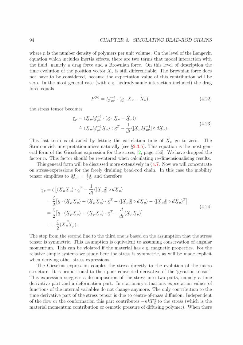
94 CHAPTER 4. SIMULATING BEAD-ROD CHAINS
where n is the number density of polymers per unit volume. On the level of the Langevinequation which includes inertia effects, there are two terms that model interaction withthe fluid, namely a drag force and a Brownian force. On this level of description thetime evolution of the position vector X
¯ν is still differentiable. The Brownian force does
not have to be considered, because the expectation value of this contribution will bezero. In the most general case (with e.g. hydrodynamic interaction included) the dragforce equals
F¯
(h) = M¯
−1µν · (κ¯ ·X¯ ν − X
¯ν), (4.22)
the stress tensor becomes
τ¯
p = 〈X¯
µM¯
−1µν · (κ¯ ·X¯ ν − X
¯ν)〉
.= 〈X
¯µM
¯−1µνX¯
ν〉 : κ¯
T − 1
dt〈[X
¯µM
¯−1µν ] dX
¯ν〉.
(4.23)
This last term is obtained by letting the correlation time of X¯
ν go to zero. TheStratonovich interpretation arises naturally (see §2.3.5). This equation is the most gen-eral form of the Giesekus expression for the stress, [2, page 156]. We have dropped thefactor n. This factor should be re-entered when calculating re-dimensionalising results.
This general form will be discussed more extensively in §4.7. Now we will concentrateon stress-expressions for the freely draining bead-rod chain. In this case the mobilitytensor simplifies to M
¯µν = 1
ζδ¯, and therefore
τ¯
p = ζ[〈X
¯µX
¯µ〉 · κ
¯T − 1
dt〈[X
¯µδ¯] dX
¯µ〉
=ζ
2
[κ¯· 〈X
¯µX
¯µ〉+ 〈X
¯µX
¯µ〉 · κ
¯T − 〈[X
¯µδ¯] dX
¯µ〉 − 〈[X
¯µδ¯] dX
¯µ〉T]
=ζ
2
[κ¯· 〈X
¯µX
¯µ〉+ 〈X
¯µX
¯µ〉 · κ
¯T − d
dt〈X¯
µX¯
µ〉]
≡ −ζ2〈X¯
µX¯
µ〉5
.
(4.24)
The step from the second line to the third one is based on the assumption that the stresstensor is symmetric. This assumption is equivalent to assuming conservation of angularmomentum. This can be violated if the material has e.g. magnetic properties. For therelative simple systems we study here the stress is symmetric, as will be made explicitwhen deriving other stress expressions.
The Giesekus expression couples the stress directly to the evolution of the microstructure. It is proportional to the upper convected derivative of the ‘gyration tensor’.This expression suggests a decomposition of the stress into two parts, namely a timederivative part and a deformation part. In stationary situations expectation values offunctions of the internal variables do not change anymore. The only contribution to thetime derivative part of the stress tensor is due to centre-of-mass diffusion. Independentof the flow or the conformation this part contributes −nkTδ
¯to the stress (which is the
material momentum contribution or osmotic pressure of diffusing polymer). When there

4.5. THE STRESS TENSOR 95
is no flow, then there is only a time derivative part. This is the case for a relaxing chain.If the flow is abruptly turned of the deformation part will disappear instantaneously.The time derivative part will however also change instantaneously. Although the micro-structure itself can not change instantaneously, the rate of change does. The deformationpart is not the same as a viscous stress.
A different stress expression can be obtained if the evolution equation Eq. (4.7)is inserted. Instead of the hydrodynamic drag force all the terms that balance it areinserted
τ¯
p =
⟨[X¯
µδ¯] 1
dt
(P¯
µν · κ¯·X
¯νdt− [δ
¯δµν − P
¯µν ]
√2dW
¯ν
)⟩
= 〈X¯
µP¯
µνX¯
ν〉 : κ¯
T 1
dt〈[X
¯µP¯
µν ] √
2dW¯
ν〉
+− 1
dt〈[X
¯µδ¯] √
2dW¯
µ〉
= 〈X¯
µP¯
µνX¯
ν〉 : κ¯
T +1
dt〈[X
¯µP¯
µν ] √
2dW¯
ν〉 − [(N + 1)δ¯− P
¯µµ]
= 〈Q¯
iQ¯
i[G−1ij Q
¯j · κ
¯·Q¯
j ]〉+ 1
dt〈[Q
¯iQ¯
iG−1ij Q
¯j ] √
2[dW¯
j − dW¯
j−1]〉− [(N + 1)δ
¯− P
¯µµ]
= τ¯
visc + τ¯
elast + τ¯
mom
(4.25)
This stress expression is the well known Kramers expression [2, page 156]. This is theexpression that is most often derived by using the more intuitive approach discussed in§4.5. For the freely draining Kramers chain this stress is naturally decomposed into threeparts. The first part is called the viscous part the second the elastic part of the stress.They represent momentum flux transported through the chain contour. Both have theform of tension times direction (all evaluated at the midpoint of a time interval). Ifthe flow is stopped abruptly, the viscous part disappears. The elastic part of the stressdoes not change instantaneously. The third part of the stress can be identified as thematerial momentum flux. This is the mean source of stress in e.g. an ideal gas. Inequilibrium the contribution of this part is −(2
3N + 1)nkTδ
¯. In non-equilibrium cases
this stress contribution becomes anisotropic, but the trace is still −(2N + 3)nkT (usingTr(P
¯µµ) = N). This is related to the number of degrees of freedom, namely the number
of beads minus the number of constraints. The viscous stress will of coarse be zero inequilibrium, the elastic stress is 2
3Nδ
¯.
4.5.3 Computing stresses
As might be clear from the preceding section, stresses can be straight forwardly calcu-lated from terms that are already available from solving the evolution equation. Manyexpressions will have contributions which are expectation values of terms proportionalto ∆W/∆t. The Ito-part of such an expression has expectation value zero. As dis-cussed in §2.5.4, such terms have a variance proportional to 1/∆t. When approximating

96 CHAPTER 4. SIMULATING BEAD-ROD CHAINS
these terms by statistical averaging over a finite number of realisations N , the errorin this estimate of the expectation value (which should be zero) will be proportionalto 1/
√N∆t. It is therefore important to eliminate this term. The needed correction
term can be obtained from the first Ito-predictor step in the algorithm for solving theevolution equation, Eq. (4.12).
For example when calculating the elastic stress, the expression one wants to approx-imate is
τ¯
elast =1
dt〈[Q
¯iQ¯
iG−1ij Q
¯j ] √
2[dW¯
j − dW¯
j−1]〉.=
1
∆t〈Q¯
(MID)i Q
¯
(MID)i G−1
ij (Q¯
(MID)j ·∆Q
¯j)〉EST
=1
∆t〈∑
i
Q¯
(MID)i Q
¯
(MID)i w
(MID)i 〉EST,
(4.26)
here Q¯
j only contains the unconstrained stochastic move, and the wi from Eq. (4.13)
is referred to as w(MID)i . This expression will diverge for ∆t → 0, the corresponding
Ito term (using quantities defined in Eq. (4.13)), with expectation value zero should besubtracted, thus
τ¯
elast.=
1
∆t〈−∑
i
Q¯
iQ¯
iwi +∑
i
Q¯
(MID)i Q
¯
(MID)i w
(MID)i 〉EST. (4.27)
There is no O(1/√
∆t) term in this expression.Exactly the same procedure can be used for the momentum contribution of the stress.
Because of the simple form of this expression it is however easy to evaluate the O(1)term explicitly. This gives
τ¯
mom.= −(N + 1)δ
¯+
1
2∆t〈∑
i
(wiQ¯
i − wi−1Q¯
i−1)(wiQ¯
i − wi−1Q¯
i−1)〉EST (4.28)
The Giesekus expression, Eq. (4.24), might seem the most straightforward stress ex-pression to evaluate. Indeed it is. Many authors have used the Giesekus expression forstationary stress calculations only. Their argument is that the time derivative can notbe evaluated because single realisations are not differentiable (see e.g. [9, page 261]).Expectation values are however differentiable. The problem is that estimated expecta-tion values of these time derivatives have the usual O(1/
√N∆t) error, if no variance
reduction is used. The variance reduced expression is
d
dt〈X¯
µX¯
µ〉 .= 〈X¯
µ(t+ ∆t)X¯
µ(t+ ∆t)−X¯
µ(t)X¯
µ(t)−[X¯
µ(t)∆X¯
(PRED)µ + ∆X
¯(PRED)µ X
¯µ(t)]〉EST.
(4.29)
No detailed knowledge of the evolution equation is needed other than that there isa constant isotropic mobility tensor. In the case of a algorithm defined in terms ofconnector vectors the midpoint is split off, which means a contribution to the stress of−δ
¯is missing. This gives (in pseudo Fortran code)
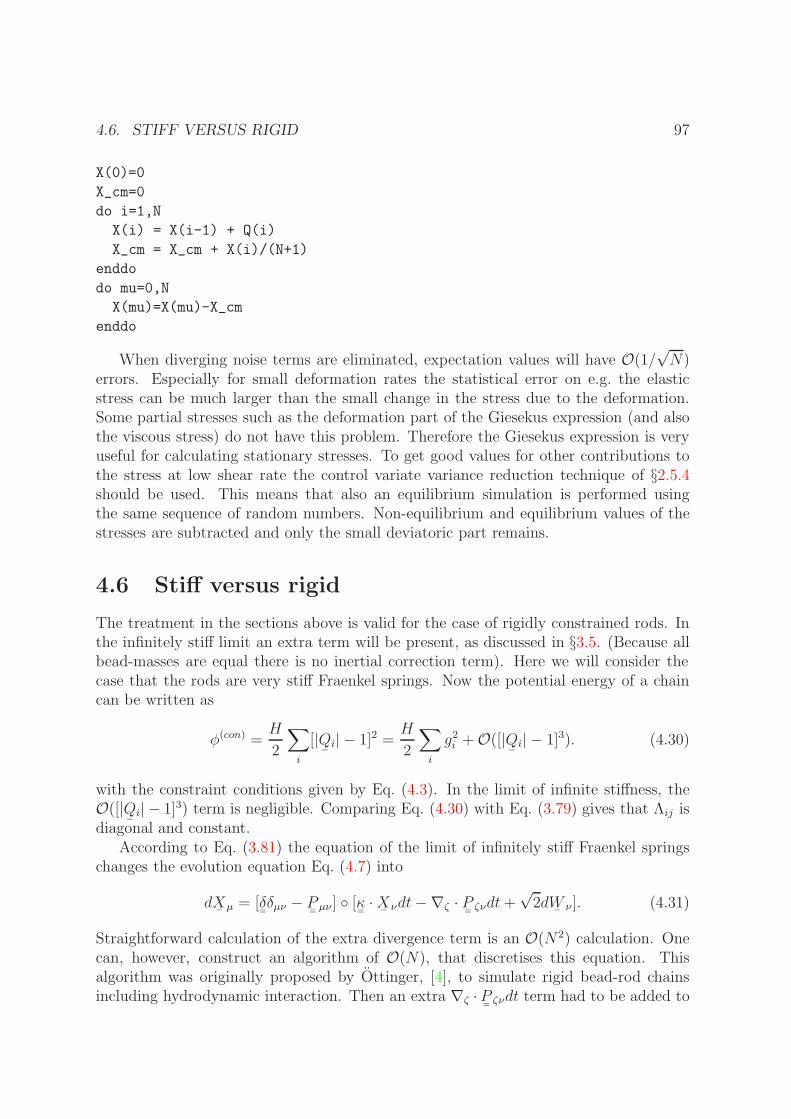
4.6. STIFF VERSUS RIGID 97
X(0)=0
X_cm=0
do i=1,N
X(i) = X(i-1) + Q(i)
X_cm = X_cm + X(i)/(N+1)
enddo
do mu=0,N
X(mu)=X(mu)-X_cm
enddo
When diverging noise terms are eliminated, expectation values will have O(1/√N)
errors. Especially for small deformation rates the statistical error on e.g. the elasticstress can be much larger than the small change in the stress due to the deformation.Some partial stresses such as the deformation part of the Giesekus expression (and alsothe viscous stress) do not have this problem. Therefore the Giesekus expression is veryuseful for calculating stationary stresses. To get good values for other contributions tothe stress at low shear rate the control variate variance reduction technique of §2.5.4should be used. This means that also an equilibrium simulation is performed usingthe same sequence of random numbers. Non-equilibrium and equilibrium values of thestresses are subtracted and only the small deviatoric part remains.
4.6 Stiff versus rigid
The treatment in the sections above is valid for the case of rigidly constrained rods. Inthe infinitely stiff limit an extra term will be present, as discussed in §3.5. (Because allbead-masses are equal there is no inertial correction term). Here we will consider thecase that the rods are very stiff Fraenkel springs. Now the potential energy of a chaincan be written as
φ(con) =H
2
∑i
[|Q¯
i| − 1]2 =H
2
∑i
g2i +O([|Q
¯i| − 1]3). (4.30)
with the constraint conditions given by Eq. (4.3). In the limit of infinite stiffness, theO([|Q
¯i| − 1]3) term is negligible. Comparing Eq. (4.30) with Eq. (3.79) gives that Λij is
diagonal and constant.According to Eq. (3.81) the equation of the limit of infinitely stiff Fraenkel springs
changes the evolution equation Eq. (4.7) into
dX¯
µ = [δ¯δµν − P
¯µν ] [κ
¯·X
¯νdt−∇ζ · P
¯ζνdt+
√2dW
¯ν ]. (4.31)
Straightforward calculation of the extra divergence term is an O(N2) calculation. Onecan, however, construct an algorithm of O(N), that discretises this equation. Thisalgorithm was originally proposed by Ottinger, [4], to simulate rigid bead-rod chainsincluding hydrodynamic interaction. Then an extra ∇ζ ·P
¯ζνdt term had to be added to

98 CHAPTER 4. SIMULATING BEAD-ROD CHAINS
obtain the rigid case. The algorithm of Ottinger is therefore not very suited to simulatethe rigid limit case, but is suited to simulate the stiff limit.
This algorithm is discussed in appendix 4.A.2. The projector operator is evaluatedat half of the unconstrained step characterised by Q
¯i + 1
2∆Q
¯i. The constraints are
obeyed to within a user specified accuracy, and determined by a recursive algorithm. Tobe able to determine stresses accurately an Ito-step has to be performed initially. Thestress can then be determined by using the Giesekus expression. If one only needs theelastic stress the best method is to subtract the viscous stress. Because the projectionoperator is evaluated at the midpoint of the unconstrained move, the terms needed forreal midpoint evaluation are not available (without doing an extra computational step).Therefore explicit computation of the elastic stress will be more expensive.
A standard result from the statistical mechanics of bead-spring chains in equilibriumis that the configurational statistics of segments are uncorrelated. This can be easilyverified by noting that the Boltzmann factors can be factorised in this case. This meansfor example that for rods i 6= j
〈(Q¯
i ·Q¯
j)2〉(STIFF) = 〈Q
¯iQ¯
i〉 : 〈Q¯
jQ¯
j〉 =(13δ¯
):(13δ¯
)=
1
3(4.32)
This is not the case for the rigid bead-rod chain. A well know result for three-bead-two-rod chain is
p(θ) ∝ sin(θ)
√1− 1
4cos2(θ), (4.33)
for the probability distribution function of the included angle (see e.g. [12]). This indi-cates that perpendicular configurations are a bit more preferred than compared to theisotropic configuration. For this case
〈(Q¯
i ·Q¯
j)2〉 = 0.32102. (4.34)
We performed variate control simulations using the rigid rod algorithm and the stiffrod algorithm simultaneously. In Fig. 4.3 the time evolution of 〈(Q
¯i · Q
¯j)
2(STIFF) − (Q
¯i ·
Q¯
j)2(RIGID)〉 is plotted. The initial configuration is a random walk configuration. For
the stiff constraints the statistics remains equal to the random walk statistics. For thethree-bead-two-rod case we indeed find that this difference equals the analytic value(which is 0.0123). For longer chains the nearest neighbour correlation in the rigid caseseems to deviate even a bit more from the random walk statistics than the two-rod case.We also found that this correlation is independent of the position along the contour.For next nearest neighbours the deviation from the uncorrelated statistics is almostnegligible. The conclusion is that the difference between stiff and rigid is only relevantwhen considering phenomena on a rod length scale. Because we are mainly interestedin long chain behaviour we will continue with using the rigid limit.

4.7. HYDRODYNAMIC INTERACTION 99
h(Q
i Q
i+2)2(STIFF) (Q
i Q
i+2)
2(RIGID)i
2 rods
64 rods
64 rodsh(Q
i Q
i+1)2(STIFF) (Q
i Q
i+1)
2(RIGID)i
time
h(Q iQ j)2 (STIFF)(Q
iQ j)2 (RIGID)i
21.510.50
0.02
0.015
0.01
0.005
0
Figure 4.3: At rod length scales there is a difference between chains consisting of infinitely stiff rodsand rigid rods. In equilibrium the inner products of neighbouring rods will be zero on average. Lookingat the square of the inner product reveals a small bias towards perpendicular conformations in the rigidcase.
4.7 Hydrodynamic interaction
When rigorously including hydrodynamic interaction most of the formalism presentedin the previous chapter should be used to its full extend. The quantity that has to beidentified is the generalised mobility tensor.
When beads move they induce a flow field. All the other beads feel this flow fieldand react appropriately. To be able to include this effect in the mobility tensor, theinteraction between beads has to be instantaneous. This means that the characteristictime scale for the hydrodynamic interaction should be much smaller than the charac-teristic time scale of a signal that propagates along the contour length. A characteristicmicro time scale for the Kramers chain is b2ζ/kT , where ζ according to the Stokes draglaw will scale with ηb. The induced flow field will propagate by diffusion through thesolvent. The appropriate diffusivity is the kinematic viscosity η/ρ. So the time neededto approximately propagate a Kuhn step is b2ρ/η. Dividing the two time steps gives
τhydr
τchain=ρkT
η2b≈ 10−9 (4.35)
for a physical realistic system.This seems a good approximation of instantaneously. There might however be a
subtlety involved. The momentum relaxation time is also a small time. It only differsfrom the characteristic time for hydrodynamic interaction in the fact that not the densityof the fluid but that of the beads should be used. These densities might be not to0

100 CHAPTER 4. SIMULATING BEAD-ROD CHAINS
far apart, which means there is no large gap in the hydrodynamic time scale and themomentum relaxation time scale. Therefore to consider hydrodynamic interaction asinstantaneous might not be totally justified. On the other hand, the beads are onlya modelling tool. It does not make much physical sense to be too critical about thedetails of the model at this scale. Only consistency conditions, such as the fluctuation-dissipation theorem remain important. In the literature on kinetic modelling of polymerchains the hydrodynamic interaction is therefore always taken to be instantaneous.
In other simulation techniques such as dissipative particle dynamics hydrodynamicinteraction is accounted for implicitly, because also the solvent is simulated. There ishowever a problem. Solvent particles are made to interact via a soft potential. Becausethe time scale corresponding to the motion of the dissipative particles is quite large, theflow field develops unrealisticly slow in such a simulation. An indication for this is theSchmidt number, this is the quotient of the diffusivity (of a fluid particle) divided by thekinematic viscosity. In a normal liquid this number is O(103), for dissipative particledynamics it is order O(1), which is a value more appropriate for gases not liquids. Manyresearchers call it a pro that the hydrodynamic interaction does not have to be modelledexplicitly in these approaches. The fact that it is not handled correctly might be a severedrawback.
In the limit of infinitely fast developing flow fields we have Stokes flow. The velocityof a (unconstrained, non-Brownian) bead is a linear function of the forces on all otherbeads, and on itself
X¯
µ = M¯
µν · F¯
ν
=1
ζ(δ¯δµν + Ω
¯µν) · F
¯ν .
(4.36)
The simplest approximation for the tensor Ω¯
µν is the Oseen-Burgers tensor. This tensorhas the problem that the mobility is not positive always. It can therefore not be usedin Brownian dynamics simulations without a modification. The most popular modifiedform for the tensor is the Rotne-Prager-Yamakawa tensor [13, page 186].
The evolution equation to be discretised is Eq. (3.36), which in the mixed index-vector notation becomes
dX¯
µ = [M¯
µη −M¯
µξ · [M¯
−1(P )]ξζ ·M
¯ζη]
[M¯
−1ην · κ¯ ·X¯ νdt+ [δ
¯δηρ − P
¯ηρ] ·
√2M
¯−1ρν · dW¯ ν ].
(4.37)
This equation can be discretised with relative ease. The performance is however verylow. At first glance the algorithm might be expected to be O(N2). Because of the hy-drodynamic interaction every bead interacts with every other bead in the chain. Due tothe random term the algorithm becomes O(N3). The cause for this is that
√M¯
−1ρν ·dW¯ ν
has to be determined. To be able to do this, the mobility tensor has to be decomposedby Cholesky decomposition, which is an O(N3) operation. In bead-spring chain simula-tions, with hydrodynamic interaction included, one often cuts costs by not performingthis decomposition each time step. The rationale is that the hydrodynamic interactiondoes not change much if the configuration of a chain only changes a little.
4.7. HYDRODYNAMIC INTERACTION 101
Aside from the fact the computation is expensive, numerical implementation ofEq. (4.37) is straightforward. As in the freely draining algorithm it consists of an Itopredictor step, a corrector step and a step to prevent the movement away from the ad-missible space caused by discretisation errors. The stress can be calculated using thegeneral Giesekus expression Eq. (4.23). Again only terms already available from the so-lution of the evolution equation have to be used. No numerically troublesome derivativeterms that arise in Ito-expressions are needed. We will not treat the algorithm in detailbecause we did not actually implement it. In literature several algorithms to includehydrodynamic interaction are proposed. These algorithms are discussed in appendix4.A.2. There we will also discuss some details of the algorithm proposed above.

102 CHAPTER 4. SIMULATING BEAD-ROD CHAINS
4.A Algorithms proposed in literature
The general algorithm for simulating bead-rod chains consists of two parts namely theevolution equation and the calculation of the stress. In this appendix we will primarilydiscuss the discretisation of the evolution equation. First we will determine whether adiscretisation of the evolution equation is valid (or is not in some cases where hydrody-namic interaction is included). Finally we will discuss what we believe are the strongand weak points of a specific algorithm. In some cases we will also indicate possibleimprovements. The way the stress computation is handled (or might be handled) is animportant issue. Both, algorithms for freely draining bead-rod chains and for chainswith hydrodynamic interaction are discussed. The discussion of the first class of algo-rithms is most relevant for comparison with the work on the freely draining bead-rodchain, presented in this and the next chapter. The second class is interesting in view ofthe general theory for constrained Brownian motion presented in the previous chapter.Many proposed algorithms will turn out to be no proper discretisations of the underlyingequations.
4.A.1 Freely draining bead-rod chains
All algorithms for freely draining bead-rod chains proposed in literature use the Lagrangemultiplier formalism to impose constraints. Sometimes the language is more ‘physical’;instead of determining Lagrange multipliers the authors try to find the tension in therods. The difference between the algorithms for the evolution equation can be foundin two aspects. Firstly the pre-factor of the multipliers can be evaluated at differenttimes (beginning of time interval or midpoint). Secondly the methods to impose theconstraints differ. This method has to be such that the evolution equation is obeyedeach time step (within discretisation errors), but also the drift away from the admissiblespace (due to an accumulation of discretisation errors) should be prevented.
In discussing the algorithms we will often use the somewhat abstract notation ofchapter 3. This avoids the, sometimes tiresome appearance, of many indices indicatingthe beads. In this setting the general, dimensionless, equation for freely draining bead-rod chains has the form of Eq. (3.37):
dX¯
= [δ¯− P
¯] [F
¯· dt+
√2 · dW
¯]. (4.38)
The force term does not only model the force but also the deterministic κ¯·X
¯ν term.
Liu
The paper of Liu [7] is one of the most well known papers on simulation of bead-rodchains. The simulation results in his paper are all for stationary flow (not withoutreason, as will be discussed below), for relatively short chains (10 to 20 beads). The

4.A. ALGORITHMS PROPOSED IN LITERATURE 103
Liu-algorithm is given by:
X¯
(n+1) = X¯
(n) + ∆X¯
(n)
= X¯
(n) + ∆X¯
(n) −∇gi∆λi
= X¯
(n) + [F¯
(n)∆t+√
2∆W¯
(n)]−∇gi∆λi,
(4.39)
where the tilde indicates the unconstrained move, and the superscripts n indicate thetime step. The N variables ∆λi are the Lagrange multipliers. Liu demands that theseare such that the constraint conditions are obeyed exactly (to within a user suppliedaccuracy), i.e. gj(X
¯(n+1)) = 0, for all i. How he handles this will be discussed in a
short while. The important thing to note in the algorithm is that all quantities areevaluated at the beginning of the time interval. This might be suspicious (consideringIto-Stratonovich subtleties), but turns out to be correct.
To check whether the algorithm is a discretisation of the correct formula we canstate the problem a bit more formal. The limit of ∆t → 0 has to be considered, whereone should take care that all terms of both O(
√∆t) and O(∆t) are modelled correctly.
In this limit the problem of finding the Lagrange multiplier is equivalent to finding avector spanned by ∇g1, . . . ,∇gNc, such that the constraint conditions are obeyed.This means we have to find P
¯· dY
¯
dX¯
= dX¯− P
¯· dY
¯, (4.40)
such the constraint conditions are obeyed
0 = gj(X¯
+ dX¯
) = ∇gj(X¯
) dX¯, ∀j ∈ 1, . . . , Nc. (4.41)
This demand is equivalent to
0 = P¯ dX
¯= P
¯· dX
¯+
1
2dX
¯dX
¯: ∇P
¯(4.42)
Substituting Eq. (4.40) in the first term on the left-hand-side gives
P¯· dY
¯= P
¯· dX
¯+
1
2dX
¯dX
¯: ∇P
¯. (4.43)
Using this relation recursively it is straightforward to find the Ito stochastic differentialequation for dX
¯and we find
dX¯
= [δ¯− P
¯] · [F
¯dt+
√2dW
¯]− 1
2dX
¯dX
¯: ∇P
¯= [δ
¯− P
¯] · [F
¯dt+
√2dW
¯]− [δ
¯− P
¯] : ∇P
¯dt
= [δ¯− P
¯] · [F
¯dt+
√2dW
¯]− P
¯· [∇ · P
¯]dt.
(4.44)
This equation is equivalent to Eq. (3.37) and we conclude that the Liu-algorithm cor-rectly discretises that equation.

104 CHAPTER 4. SIMULATING BEAD-ROD CHAINS
To satisfy the constraint conditions of constant rod lengths, Liu uses an iterativescheme. To see how this scheme works we have to turn to the index notation (using theconnector vectors). The equation for a connector vector reads
Q¯
(n+1)i = Q
¯
(n)i + ∆Q
¯
(n)i −∆λj [2δij − δi−1,j − δi,j−1]Q
¯
(n)j . (4.45)
This shows very clearly that the values of ∆λj are something like a tension. The con-
straint conditions |Q¯
(n+1)i | = 1 give a quadratic equation for the ∆λj. Using this expres-
sion Liu found the following iterative scheme for ∆λj
2
[2δij − δi−1,j − δi,j−1]Q
¯
(n)j · (Q
¯
(n)i + ∆Q
¯
(n)i )
∆λj :=
(|Q¯
(n)i + ∆Q
¯
(n)i |2 − 1) + |∆λk[2δik − δi−1,k − δi,k−1]Q
¯
(n)k |2. (4.46)
The iteration stops if the constraint condition is obeyed to within a specified accuracy.The matrix on the left-hand side is a (non-symmetric) tridiagonal matrix. It thereforeonly costs O(N) operations to invert. Furthermore the matrix does not change duringthe iteration process. This means it only has to be factorised once, making the operationvery efficient. The first term on the right-hand side is also constant. The second term hasto be recalculated every time step, but also this is a cheap O(N) operation. Liu reportsthat the iterative procedure converges quickly. According to [10], 6 to 15 iterations areneeded.
To calculate the stress Liu uses the Giesekus expression, Eq. (4.24). He only con-siders stationary stresses, and thus discards the time derivative part. The ‘deformation’part of the Giesekus expression is easily calculated and has no O(1/∆t) noise arises.He could have obtained the time derivative part too, just by calculating [〈X
¯µX
¯µ〉(n) −
〈X¯
µX¯
µ〉(n+1)]/∆t. This term does have O(1/[N∆t]) noise (N is the number of realisa-tions, not the rods). To obtain stationary results Liu uses a time averaging. He did notintroduce variance reduction methods to get rid of the (diverging) noise.
Probably the strong part of the Liu algorithm is the efficiency (although we thinkour algorithm is cheaper). The occurrence of computationally more expensive operationsis minimised. Only once each time step a non-symmetric tridiagonal matrix has to befactorised. The weak point has to do with the stress calculation. In this form of thealgorithm information needed to do variance reduced stress calculations is not available.Therefore stress computation, without using a large number of realisations, can onlybe performed for stationary situations. The work of Doyle et al. ([9], [14] and [15])uses the algorithm of Liu as a basis, but extends the stress calculation to non-stationarysituations.
Grassia and Hinch
The algorithm presented by Grassia and Hinch is very similar to the algorithm wepresented. It is also a straightforward midpoint implementation of the Stratonovichequation Eq. (4.38). The first step is a predictor step to predict the midpoint with

4.A. ALGORITHMS PROPOSED IN LITERATURE 105
order√
∆t accuracy. The second step is a corrector step using the information at themidpoint to get a O(∆t) accurate implementation. The difference is the method tosuppress numerical drift. The way they prevent the increase of the lengths of the rodsdue to discretisation errors is by renormalising the connector vectors. If the length of arod deviates 0.5% from 1 the connector vector is divided by its length.
That this is a very dangerous procedure is illustrated in Fig. 4.4. Here time depen-dence of the end-to-end distance in equilibrium for an ensemble of chains of 32 rods isshown. Subsequent to every Stratonovich time step, the rods are renormalised to unitlength. The end-to-end distance increases dramatically beyond the theoretical value of√N . The reason for this is intuitively clear.
The numerical discretisation error is bound to have a systematic effect on the con-tour length (in this case decreasing it). Perturbations will most probably have localeffects on the contour length. Brownian motion of a specific bead will (by means of thediscretisation error) influence the length of neighbouring rods most. Large length scalestructures such as the end-to-end distance will be influenced much less. When rescalingthe contour length by dividing the connector vectors through there lengths, all lengthscales are influenced equally. This causes the end-to-end to deviate from the theoreticalvalue.
This effect will of course decrease with decreasing time steps. However Fig. 4.4shows that the effect is quite large. Our opinion is that it is so large that the algorithmof Grassia and Hinch can not be used for simulations where large length scales aredominant in the dynamics. This will be the case in the near equilibrium regime. Herethe dominant length and time scale as that of the coil. Also shown in the figure is theimplementation of our algorithm (see §4.4) which is completely equivalent to theirs inthe Stratonovich part, but handles the suppression of the drift from the admissible spacedifferently. Although we do not rigorously require the contour length to be constant,the deviation is extremely small. Moreover there is no drift in the end-to-end distancewhatsoever.
The major contribution, as far as development of the algorithm is concerned, ofthe paper of Grassia and Hinch is the stress computation. They calculate both themomentum flux contribution and the elastic contribution to the stress using variancereduction methods. The way this is presented in their paper does, however, make thispoint not very explicit. We will present their procedure using the ‘bead-rod’-notation.When discussing the evolution equation they redefine the ‘random’ forces as
F¯
raµ = [δ
¯δµν − P
¯µν ] · F
¯ra (uncon)ν
.=
1
∆t[δ¯δµν − P
¯µν ] ·√
2∆W¯
ν . (4.47)
These random forces can be obtained by performing one predictor step in the algorithm.As is clear from Eq. (3.37) the redefined random forces give exactly the same evolution(and thus, by means of the Giesekus expression, the same stresses). The stresses can be

106 CHAPTER 4. SIMULATING BEAD-ROD CHAINS
30
40
50
60
70
80
90
0 0.01 0.02 0.03 0.04 0.05
⟨R2 ⟩
t ∆t
Grassia and Hinch, ∆t=0.010Grassia and Hinch, ∆t=0.005
present results, ∆t=0.010present results, ∆t=0.005
31.9996
31.9998
32
32.0002
32.0004
32.0006
32.0008
0 0.01 0.02 0.03 0.04 0.05
cont
our
leng
th
t ∆t
Grassia and Hinch, ∆t=0.010Grassia and Hinch, ∆t=0.005
present results, ∆t=0.010present results, ∆t=0.005
Figure 4.4: Equilibrium simulation of (1000) bead-rod chains with 32 segments. The renormalisationof the connector vectors in the algorithm of Grassia and Hinch increases the end-to-end distance.

4.A. ALGORITHMS PROPOSED IN LITERATURE 107
calculated using this redefined force. The momentum contribution is
τ¯
mom = −〈X¯
µδ¯ F
¯raµ −X¯ µF
¯raµ 〉EST
= − 1
∆t〈X¯
µδ¯ [δ
¯δµν − P
¯µν ] ·√
2∆W¯
ν
−X¯
µ[δ¯δµnu − P
¯µν ] ·√
2∆W¯
ν〉EST .
(4.48)
Here the stochastic part is zero, therefore there is no diverging noise. The elastic partthey calculate as
τ¯
elast = 〈X¯
µP¯
µν F¯
raν 〉EST . (4.49)
Also here the stochastic part is zero, because P¯
µν · F¯
raν = 0. Here it is essential that
the redefined instead of the original random forces are used. Because Grassia and Hinchonly consider the problem of relaxation (i.e. no flow) they do not give an expression forthe viscous contribution to the stress.
Doyle et al.
Doyle et al. have a series of papers on simulations of Kramers chains, [9], [14] and [15].Their main new contributions are the monitoring of birefringence and the analysis of thedecomposition of the stress in a elastic (which they call Brownian) and a viscous part.They elaborate on the algorithm of Liu. Their contribution to the development of thealgorithm is mainly the method to calculate stresses in transient flow.
In their first paper, [9], Doyle, Shaqfeh and Gast introduce a method to calculatestresses avoiding the O(1/(N∆t)) noise, which they call noise reduction. The do notidentify this as a special case of variance reduction. They e.g. write that the Giesekusexpression (Eq. (4.24)) for the stress can not be used in transient situations, becausetrajectories are not differentiable [9, page 254]. This statement is not true. It is truethat individual trajectories are not differentiable, but the differential of a expectationvalue exists. The naive numerical approximation of this differential has an error ofO(1/(N∆t)), equivalently to naive calculations of the decomposed stresses. Using thesame variance reduction method for this time derivative as for the decomposed stresscomponents gives a signal with O(1) non-diverging noise.
The original Liu algorithm is not very well suited for these variance reduction meth-ods. This is because the method requires an Ito step. Already the first iteration step ofthe Liu iteration scheme Eq. (4.46) gives rise to contributions in the Lagrange multipli-ers ∆λj of order ∆∆Q
¯
2i . Therefore, even if only the stochastic contribution to ∆Q
¯i is
considered, the expectation values of the Lagrange multipliers are not zero, and can notbe used for variance reduction.
To obtain an Ito-step, the equation has to be linearised in ∆Q¯
i, this gives Eq. (4.12),with the symmetric tridiagonal matrix Gij which has to be inverted. Doyle et al. use thislinearised scheme once (using only the Brownian displacement) to obtain the Ito-steprequired to do variance reduction (it gives the term P
¯µν ·√
2∆W¯
ν). They also use thisscheme once with only the deterministic flow term. This enables them to calculate the

108 CHAPTER 4. SIMULATING BEAD-ROD CHAINS
viscous part of the stress. The final total displacement is found by iteration using theLiu scheme.
Their variance reduced form of the elastic stress tensor ([9] Eq.(5.9)), when there isno flow, looks like
τ¯
elast = − 1
∆t
⟨[X¯
µP¯
µν ] √
2∆W¯
ν − [X¯
µδ¯] (P
¯µν ·√
2∆W¯
ν)
+
[X¯
µδ¯] (P
¯µν ·√
2∆W¯
ν)−X¯
µ · P¯
µν ·√
2∆W¯
ν⟩
EST
.= − 1
∆t
⟨1
2[X¯
(n+1)µ +X
¯(n)µ ][∆X
¯µ −∆X
¯µ]
− 1
2[X¯
(n+1)µ +X
¯(n)µ ](P
¯µν ·√
2∆W¯
ν)
+1
2[X¯
(n+1)µ −X
¯(n)µ ](P
¯µν ·√
2∆W¯
ν)⟩
EST
.
(4.50)
In the presence of a flow field present this gives the elastic plus the viscous stress. Ascan be seen most easily from the first expression there are some redundant terms. Thestochastic part is zero and thus the variance does not diverge with decreasing step size.The way Doyle et al. calculate the elastic stress is by subtracting the viscous stress.
The authors missed out on the anisotropic momentum flux part. It is surprising tosee that the above calculation is almost a variance-reduced calculation of the stress usingthe Giesekus expression. Something the authors say is not possible. If they had used thefull Giesekus expression, i.e. not subtracting the unconstrained increment, they wouldalso have included the anisotropic momentum contribution.
Similarly to the algorithm of Grassia and Hinch, the main contribution of the Doylealgorithm is the possibility of variance reduced computation of stresses, this makesnon-stationary calculations possible. The modification of Doyle et al. to the algo-rithm of Liu makes the algorithm considerably more expensive. The beauty of theLiu-algorithm is that the (tridiagonal) matrix only has to be decomposed once. In theDoyle-algorithm there are two matrices. The ‘Liu-matrix’ and the symmetric tridiago-nal matrix Gij, which is needed to calculate the Ito-step. The elegance and efficiency ofthe Liu-algorithm are lost. Nevertheless, it is better to lose elegance than to introduceserious discretisation errors as is the case of the Grassia and Hinch algorithm.
If we were to suggest an alteration to possibly improve to this, it would be a mi-nor change of the Liu-algorithm. The suggestion is to put the term 2[2δij − δi−1,j −δi,j−1]Q
¯
(n)i · ∆Q
¯
(n)i ∆λj, which is on the left hand side in Liu’s scheme Eq. (4.46), to
the right-hand-side. Now, the matrix to be inverted is Gij , evaluated at the beginningof a time interval. The newly proposed algorithm would consist of three steps. Firstcalculate a Brownian Ito-step. Then calculate a deterministic (linearised) step if onewants to calculate the viscous stress contribution separately. Add both increments in∆λj and finally use these values as initial values for the altered Liu-iteration process.The benefits are obvious. Only one symmetric positive definite tridiagonal matrix has to
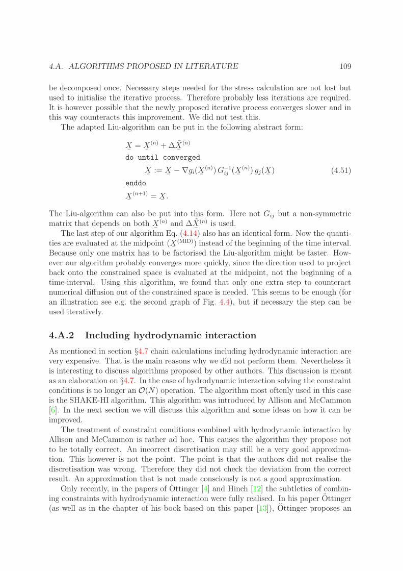
4.A. ALGORITHMS PROPOSED IN LITERATURE 109
be decomposed once. Necessary steps needed for the stress calculation are not lost butused to initialise the iterative process. Therefore probably less iterations are required.It is however possible that the newly proposed iterative process converges slower and inthis way counteracts this improvement. We did not test this.
The adapted Liu-algorithm can be put in the following abstract form:
X¯
= X¯
(n) + ∆X¯
(n)
do until converged
X¯
:= X¯−∇gi(X
¯(n))G−1
ij (X¯
(n)) gj(X¯
)
enddo
X¯
(n+1) = X¯.
(4.51)
The Liu-algorithm can also be put into this form. Here not Gij but a non-symmetricmatrix that depends on both X
¯(n) and ∆X
¯(n) is used.
The last step of our algorithm Eq. (4.14) also has an identical form. Now the quanti-ties are evaluated at the midpoint (X
¯(MID)) instead of the beginning of the time interval.
Because only one matrix has to be factorised the Liu-algorithm might be faster. How-ever our algorithm probably converges more quickly, since the direction used to projectback onto the constrained space is evaluated at the midpoint, not the beginning of atime-interval. Using this algorithm, we found that only one extra step to counteractnumerical diffusion out of the constrained space is needed. This seems to be enough (foran illustration see e.g. the second graph of Fig. 4.4), but if necessary the step can beused iteratively.
4.A.2 Including hydrodynamic interaction
As mentioned in section §4.7 chain calculations including hydrodynamic interaction arevery expensive. That is the main reasons why we did not perform them. Nevertheless itis interesting to discuss algorithms proposed by other authors. This discussion is meantas an elaboration on §4.7. In the case of hydrodynamic interaction solving the constraintconditions is no longer an O(N) operation. The algorithm most oftenly used in this caseis the SHAKE-HI algorithm. This algorithm was introduced by Allison and McCammon[6]. In the next section we will discuss this algorithm and some ideas on how it can beimproved.
The treatment of constraint conditions combined with hydrodynamic interaction byAllison and McCammon is rather ad hoc. This causes the algorithm they propose notto be totally correct. An incorrect discretisation may still be a very good approxima-tion. This however is not the point. The point is that the authors did not realise thediscretisation was wrong. Therefore they did not check the deviation from the correctresult. An approximation that is not made consciously is not a good approximation.
Only recently, in the papers of Ottinger [4] and Hinch [12] the subtleties of combin-ing constraints with hydrodynamic interaction were fully realised. In his paper Ottinger(as well as in the chapter of his book based on this paper [13]), Ottinger proposes an

110 CHAPTER 4. SIMULATING BEAD-ROD CHAINS
alternative and correct algorithm. This algorithm also seems ad hoc. At first glance itwill not be clear why it should give rise to a discretisation of the correct stochastic dif-ferential equation, but as shown by Ottinger it actually does. An important motivationto discuss the algorithm is that it is especially useful for the simulation of infinitely stiffsystems (see §4.6 for this).
Again, to keep the notation simple, we will not consider the equations for the spe-cific case of bead-rod chains, but the more general formulation of the previous chapterEq. (3.36) (masses of the beads are assumed to be equal).
Allison and McCammon
When not realising what the subtleties are when using stochastic differential equationsand not really thinking about how constraints give rise to normal forces, one does arrivequickly at an algorithm similar to the one proposed by Liu Eq. (4.39). The procedurehere is: first consider unconstrained motion, then find Lagrange multipliers such that theconstraint conditions are satisfied. Everything is evaluated at the beginning of a timeinterval. The directions that are projected back onto zero are defined by the gradientsof the constraint conditions. This means that motion in directions perpendicular to theconstrained space are projected onto zero. This is not correct because not displacementsbut normal forces are required to be perpendicular, which is not the same thing. Thenon-isotropic mobility tensor may transform a normal force to a displacement that isitself not perpendicular.
Allison and McCammon recognised this last point. In the appendix of their paper [6]they give a modified version which accounts for the fact that normal forces are needed.The normal forces are spanned by the gradients, therefore the constrained displacementsare expected to be spanned by the directions M
¯· ∇gi. Their algorithm looks like
X¯
(n+1) = X¯
(n) + ∆X¯
(n)
= X¯
(n) + ∆X¯
(n) −M¯· ∇gi∆λi
= X¯
(n) + [M¯· F¯
(n)∆t+∇ ·M¯
∆t+√
2M¯
∆W¯
(n)]−M¯· ∇gi∆λi.
(4.52)
In papers on hydrodynamic interaction the divergence term of the mobility will rarelybe found. Nevertheless most authors are aware of this term, but in the case of hydro-dynamic interaction it is zero for the most commonly used approximations. (This isconnected to the fact that the velocity field is divergence free). Although the inclusionof the mobility matrix is an improvement it is still a bit ad hoc. The common miscon-ception in these early papers is that if the constraint condition is met with a certainaccuracy, also the equation of motion would be correct within that accuracy.
To find the correct Lagrange multipliers is much more difficult for the case of hydro-dynamic interaction than for the case of freely draining bead-rod chains. The matrixthat has to be inverted is no longer a simple tridiagonal matrix such as Gij . For theseproblems the SHAKE method was developed. Here a dλi for a specific i is taken in sucha way that the corresponding constraint condition gi = 0 is satisfied. When we repeatthis same procedure for the next i, the previous constraint is not obeyed any longer. The
4.A. ALGORITHMS PROPOSED IN LITERATURE 111
procedure has to be performed iteratively and the hope is that it converges quickly. Thismight not be the case. For example for a fully stretched chain in elongational flow thenumber of iterations would be of O(N3). Our guess is that the number of iteration scalesas λ2N . Here λ is a measure that specifies the displacement along the chain contourneeded to get decorrelated orientations. This scaling means that the SHAKE algorithmbecomes as expensive, or more expensive as matrix inversion for situations where thechains are almost stretched.
The original SHAKE method [16] was introduced for the determination of Lagrangemultipliers where the mobility matrix is not present. The SHAKE algorithm for the casewhere hydrodynamic interaction plays a role is introduced in the Allison-McCammonpaper [6] and is commonly referred to as SHAKE-HI.
Our proposal to improve on this algorithm for the specific case of simulation ofchains including hydrodynamic interaction is to split the mobility tensor in a diagonalpart (this would be the bead-friction part) and an off-diagonal part (this would be thehydrodynamic interaction part). Because the constraint conditions gj(X
¯) are (in this
special case) quadratic functions of the coordinates we can write
0 = gj(X¯
(n+1)) = g(X¯
(n) + ∆X¯
)
= ∆X¯· ∇gj +
1
2∆X
¯∆X
¯: ∇∇gj
= −∆λi∇gi · ∇gj + (∆X¯−∆λk[M
¯− δ
¯] · ∇gk) · ∇gj
+1
2(∆X
¯−∆λkM
¯· ∇gk)(∆X
¯−∆λlM
¯· ∇gl) : ∇∇gj
(4.53)
The iterative scheme we suggest for solving this equality is
∆λi := G−1ij
(∆X
¯−∆λk[M
¯− δ
¯] · ∇gk) · ∇gj
+1
2(∆X
¯−∆λkM
¯· ∇gk)(∆X
¯−∆λlM
¯· ∇gl) : ∇∇gj
(4.54)
For M¯
= δ¯
this scheme reduces to the altered Liu-algorithm. For the case with hy-drodynamic interaction, our feeling is that it converges much faster than the originalSHAKE-HI algorithm, and is almost as expensive. The reason for this fast convergenceis that the interactions along the contour, which are very important in partly stretchedsituations, are handled explicitly.
To obtain the stochastic differential equation that is approximated by the algorithmof Allison and McCammon the same procedure as for the Liu-algorithm can be followed.Now the starting point will be
dX¯
= dX¯−M
¯· P¯· dY
¯= [M
¯· F¯dt+∇ ·M
¯dt+
√2M
¯· dW
¯]−M
¯· P¯· dY
¯.
(4.55)
Also here the constraint condition demands that P¯ dX
¯= 0. This gives, equivalently
to Eq. (4.43),
M¯· P¯· dY
¯= M
¯·M
¯−1(P ) · [dX¯ +
1
2dX
¯dX
¯: ∇P
¯], (4.56)

112 CHAPTER 4. SIMULATING BEAD-ROD CHAINS
and thus
dX¯
= [δ¯−M
¯·M
¯−1(P )] · dX¯ −
1
2M¯·M
¯−1(P ) · (dX¯ dX¯ : ∇P
¯)
= [δ¯−M
¯·M
¯−1(P )] · dX¯ −
1
2dX
¯dX
¯: ∇(M
¯−1(P ) ·M¯ )
= [δ¯−M
¯·M
¯−1(P )] · [M¯ · F¯dt+∇ ·M
¯dt+
√2M
¯· dW
¯]
− [M¯−M
¯·M
¯−1(P ) ·M¯ ] : ∇(M
¯−1P ) ·M¯ )dt
= [δ¯−M
¯·M
¯−1(P )] · [M¯ · F¯dt+∇ · (M
¯·M
¯−1(P ) ·M¯ )dt
+√
2M¯· dW
¯] +∇ · [M
¯−M
¯·M
¯−1(P ) ·M¯ ]dt
(4.57)
This equation is not equal to Eq. (3.36). The algorithm of Allison and McCammon istherefore not a discretisation of the correct equation.
The SHAKE-HI procedure is however a large conceptual improvement over theSHAKE algorithm. For the cases Allison and McCammon studied they report a quan-titative 5% difference between results obtained by the two different algorithms. Noqualitative differences are reported. We do not think that the difference between theiralgorithm and a correct discretisation will be large. The safest thing to do is to just usea correct discretisation as proposed in §4.7 or given by Ottinger.
Recently the Allison-McCammon algorithm has been used by Agarwal and Bhargava[17].
Ottinger
Subsequent to the derivation of the correct stochastic differential equation for constrainedmotion (see [4], [13] and appendix 3.A), Ottinger proposes an algorithm for simulatingthis equation. His proposal is a variation on the Allison-McCammon algorithm. Thereare two alterations. The first is that in the unconstrained move the “metric” force isincluded (see appendix 3.A). Therefore the unconstrained move (supposing all beadmasses equal) becomes
∆X¯
= M¯· F
¯+∇ · P
¯∆t+∇ ·M
¯dt+
√2M
¯·∆W
¯. (4.58)
The second alteration is that the vectors M¯·∆gi are not evaluated at the beginning of
a time interval but at X¯
(n) + 12∆X
¯. The algorithm is thus
X¯
(n+1) = X¯
(n) + ∆X¯
(n) − [M¯· ∇gi](X
¯(n)+ 1
2∆X¯
)∆λi. (4.59)
Ottinger does not give a real implementation of the algorithm. He supposes that theconstraints are enforced using an iterative procedure such as the SHAKE-HI algorithm.
The determination of the equation which is discretised by this algorithm is found bythe same method as used above. The infinitesimal equation can be written as
dX¯
= dX¯− [M
¯· P¯](X¯
+ 12∆X¯
) · dY¯= dX
¯− 1
2dY
¯dX
¯: ∇P
¯−M
¯· P¯· dY
¯.
(4.60)

4.A. ALGORITHMS PROPOSED IN LITERATURE 113
In this case the constraint condition P¯ dX
¯= 0 results in
M¯· P¯· dY
¯= M
¯·M
¯−1(P ) · [dX¯ −
1
2dY
¯dX
¯: (∇P
¯·M
¯) +
1
2dX
¯dX
¯: ∇P
¯], (4.61)
where
dX¯dX
¯= 2M
¯dt
dY¯dX
¯= 2M
¯−1(P ) ·M¯ dt
dX¯dX
¯= 2[M
¯−M
¯·M
¯−1(P ) ·M¯ ]dt.
(4.62)
Using these identities gives
dX¯
= [δ¯−M
¯·M
¯−1(P )] · [dX¯ −
1
2dY
¯dX
¯: ∇(P
¯·M
¯)]
−M¯·M
¯−1(P ) · [
1
2dX
¯dX
¯: ∇P
¯]
= [δ¯−M
¯·M
¯−1(P )] · [dX¯ − [M
¯−1(P ) ·M¯ ] : ∇(P
¯·M
¯)dt]
−M¯·M
¯−1(P ) · [(M¯ −M¯ ·M¯
−1(P ) ·M¯ ) : ∇P
¯]dt
= [δ¯−M
¯·M
¯−1(P )] · [dX¯ −∇ ·M¯ dt] +∇ · (M
¯−M
¯·M
¯−1(P ) ·M¯ )dt
= [δ¯−M
¯·M
¯−1(P )] · [M¯ · F¯ +∇ · P
¯dt+
√2M
¯· dW
¯]
+∇ · (M¯−M
¯·M
¯−1(P ) ·M¯ )dt
(4.63)
Comparing this expression with Eq. (3.36) shows that the algorithm proposed byOttinger is indeed a correct discretisation. The need to include the term ∇ · P
¯is less
elegant. For a bead-rod chain to calculate this term is an O(N2) operation. This mightbe thought to be negligible compared by the O(N3) operation of Cholesky decomposi-tion, which is needed when treating hydrodynamic interaction. It might however becomea leading term in the computation if the hydrodynamic interaction is not recalculatedeach time step, see §4.7.
Ottinger remarks [13, page 245] that, with leaving this additional term in, one obtainsthe stiff limit. Because there is not one stiff limit this is not true in general. The limitdepends on the stiff potential. In general also a factor 1
2∇ log(det[Λij ]) has to be included
besides ∇ · P¯, see Eq. (3.81). The functional form of the constraint conditions can be
chosen such that this additional term disappears. It turns out that for bead-rod chains,the most natural choice of constraint conditions and the most natural choice for the stiffpotential (see §4.6) coincides with the choice Λij = constant. If one wants to use a stiffinstead of a rigid system, the Ottinger algorithm is the one thing to use, but care hasto be taken in choosing the functional form of the constraint conditions.
In Ottingers algorithm the vector space which is used for the projection onto theadmissible space is sampled at X
¯+ 1
2dX
¯. This is a position outside the admissible
space. It is therefore not remarkable that there is a term needed (namely ∇ · P¯) which
corrects for the functional form of the constraint conditions. The fact that Ottingers

114 CHAPTER 4. SIMULATING BEAD-ROD CHAINS
algorithm without this term discretises a stiff system can also be understood intuitively.The midpoint evaluation is something like a Stratonovich interpretation. But becauseof the small (but not infinitely small) correlation time corresponding to the stiffness theconstraint condition does not instantaneously constrain the zero-correlated stochasticterm. Therefore the unconstrained instead of the constrained move arises in the midpointevaluation. This is however not more than a hand waving argument to explain why thealgorithm works.
In a very recent paper Petera and Muthukumar [18] presented a simulation studyof Kramers chains including hydrodynamic interaction and excluded volume. This isthe first running implementation of the Ottinger algorithm. To calculate the stressesthey use a full Ito-expression. We suspect this to be an expensive calculation. Becausea simple Ito-step is not available in the Ottinger algorithm it is somewhat difficult touse the cheaper variance reduced methods where only terms already available from theevolution equation are used, see §4.7.
To finish this appendix we will give an outline of the discretisation of Eq. (4.37). Thefirst step is the unconstrained Ito predictor step. This step has to be constrained viaEq. (4.59), but here, as in the original SHAKE-HI algorithm the term [M
¯· ∇gi] has to
be evaluated at the beginning of the time interval. An iterative procedure as discussedabove has to be used to obtain the Lagrange multipliers, O(∆t) accuracy suffices. Nowthe midpoint can be determined as
X¯
(MID)µ := X
¯µ +
1
2∆X
¯(PRED)µ
∆X¯
µ := κ¯·X
¯(MID)µ ∆t+M
¯(MID)µη · [δ
¯δηρ − P
¯ηρ] ·
√2M
¯−1ρν · dW¯ ν ].
(4.64)
This step has to be constrained by solving Eq. (4.37), but now with [M¯· ∇gi] evaluated
at the midpoint.

Bibliography
[1] H.A. Kramers. The behaviour of macromolecules in inhomogeneous flows. J. Chem.Phys., 14:415–424, 1946.
[2] R.B. Bird, C.F. Curtiss, R.C. Armstrong and O. Hassager. Dynamics of PolymerLiquids. Vol. 2. Kinetic Theory. John Wiley, New York, 2 edition, 1987.
[3] M. Fixman. Simulation of polymer dynamics. I. general theory. J. Chem. Phys.,69:1527–1537, 1978.
[4] H.C. Ottinger Brownian dynamics of rigid polymer chains with hydrodynamicinteraction. Phys. Rev. E., 50(4):2696–2701, 1994.
[5] D. Acierno, Titomanlio G. and Marrucci G. Dilute solution rheology of flexiblemacromolecules (bead-rod model). J. Polym. Sci. (Polym. Phys. Ed.), 12:2177–2187, 1974.
[6] S.A. Allison and J.A. McCammon. Transport proporties of rigid and flexible macro-molecules by Brownian dynamics simulation. Biopol., 23:167–187, 1984.
[7] T.W. Liu. Flexible polymer chain dynamics and rheological properties in steadyflow. J. Chem. Phys., 90(10):5826–5842, 1989.
[8] P. Grassia and E.J. Hinch. Computer simulations of polymer chain relaxation viaBrownian motion. J. Fluid Mech., 308:255–88, 1996.
[9] P.S. Doyle, E.S.G. Shaqfeh and A.P. Gast. Dynamic simulation of freely drainingflexible polymers in steady linear flows. J. Fluid Mech., 334:251–291, 1997.
[10] I. Ghosh, R.C. Armstrong, R.A. Brown and G.H. McKinley. Modeling dilute poly-mer solutions in extensional flows at intermediate strains. presentation, 1999.
[11] P.S. Grassia, E.J. Hinch and L.C. Nitsche. Computer simulations of Brownianmotion of complex systems. J. Fluid Mech., 282:373–403, 1995.
[12] E.J. Hinch. Brownian motion with stiff bonds and rigid constraints. J. Fluid Mech.,271:219–34, 1994.
[13] H.C. Ottinger. Stochastic Processes in Polymeric Fluids. Springer Verlag, Berlin,1996.
115

116 BIBLIOGRAPHY
[14] P.S. Doyle, E.S.G. Shaqfeh, McKinley G.H. and S.H. Spiegelberg Relaxation ofdilute polymer solutions following extensional flow. J. Non-Newtonian Fluid Mech.,76:79–110, 1998.
[15] P.S. Doyle and E.S.G. Shaqfeh Dynamic simulation of freely-draining, flexible bead-rod chains: Start-up of extensional and shear flow. J. Non-Newtonian Fluid Mech.,76:43–78, 1998.
[16] J.P. Ryckaert, G. Ciccotti and H.J.C. Berendsen Numerical integration of motionof a system with constraints: molecular dynamics of n-alkanes. J. Comput. Phys.,23:327–341, 1977.
[17] U.S. Agarwal, Bhargava R. and R.A. Mashelkar. Brownian dynamics simulation ofa polymer molecule in solution under shear flow. J. Chem. Phys., 108(4):1610–1617,1998.
[18] D. Petera and M. Muthukumar Brownian dynamics simulation of bead-rod chainsunder shear with hydrodynamic interaction. J. Chem. Phys., 111(16):7614–7623,1999.

Chapter 5
Bead-rod chains in elongational flow
5.1 Introduction
In this chapter we will investigate the behaviour of a bead-rod chain in elongational flowusing the Brownian dynamics code described in the previous chapter. There are severalreasons to look at this specific combination of flow type and polymer model. Firstly,elongational flow is important in a number of cases where dilute polymer solutionsare industrially relevant; examples being fibre spinning, turbulent drag reduction andflow through a porous medium. Secondly, the behaviour of chains in elongational flowposes many questions to the validity of more coarse grained polymer models such asdumbbell models. Lastly, experimental techniques have recently become available bywhich properties in elongational flow can be measured accurately.
Until about a decade ago the only kind of controlled extensional flow that was ac-cessible experimentally (at least for polymer solutions) was stagnation-point flow. Anexample of apparatuses which create such a stagnation point are the four roll mill andthe opposing jet device. In the stagnation point a perfect extensional flow is created.The flow field away from this stagnation point is not very well defined. It can not beprescribed a priori by means of e.g. Stokes flow because the polymer contributions tothe stress influence the flow field. Therefore one would like to measure in the stagnationpoint only. A direct measurement of the stress over there is not possible. By means ofoptical techniques the average orientation of the polymer in the stagnation point canbe measured. For solutions in strong flow there is however not a one-on-one relationbetween average orientation and stress (the so called stress-optical law is not valid).
Luckily the last decade two experimental techniques have been introduced that areable to provide very useful extensional data. The first technique is monitoring singleDNA molecules in a stagnation point. By looking at single molecules the mechanismsof unravelling in elongational flow can be tested in the most direct way. The secondtechnique is the filament stretching device. A droplet of a polymeric solution is stretchedby rapidly moving two discs apart. The force on the discs is measured. These techniques,especially the filament stretching device, produce data which can not be explained bythe commonly used constitutive equations.
117

118 CHAPTER 5. BEAD-ROD CHAINS IN ELONGATIONAL FLOW
An important goal of rheological research is to be able to understand the behaviourof a non-Newtonian fluid also in complex geometries. The fact that models that predictthe shear behaviour reasonably well can be completely off in elongational flow is badnews in this respect. In complex geometries the flow type can change in space and time.All flow types have to be described well.
The bead-rod chain is the ideal tool for an investigation of elongational flow. Thebead-rod chain is generally believed to be a reliable model for investigating rheologicalbehaviour. In experiments, polymers of different chemical compositions are found tohave similar behaviour. The bead-rod model is not so detailed that it includes chemicalinformation that is irrelevant for rheological behaviour. On the other hand the model isnot coarse grained much beyond this level.
This is different for bead-spring models. The springs are so called entropic springs.They model a mean thermodynamic force exerted by a chain segment consisting of alarge number of rods. When calculating this spring force it is assumed that many, if notall, accessible micro states are probed. For rapid deformation and large extensions thisis not the case. For elongation the situation is worse than for shear, because shear isa weak flow. The more transient and strong the elongational flow the less trustworthyentropic springs are.
One can distinguish three basic conformations of a chain. The coiled state, thestretched state and the kinked state. The main feature of coil or near coil conformationis its large number of modes. The stress is caused by a perturbations of the equilib-rium state. These perturbations decay by means of diffusion along the chain contour.The longest relaxation time, connected to long length scale deformations is, the timeneeded to diffuse the total length of the chain. Shorter lengthscale perturbations decayquicker. In section §5.3 we will investigate this conformation. We will demonstratesome Brownian dynamics simulation techniques such as variance reduction, which is es-pecially important in this near equilibrium regime. The investigation gives the spectrumof relaxation times. The Weissenberg number can be defined very accurately using thisspectrum. If the Weissenberg number is higher than one the flow is considered strongand the chain will stretch.
For the stretched or near stretched conformation the main characteristic is that thereis no characteristic time. In the stretched direction there is a balance between drag forceon the beads and the tension in the rods. In the perpendicular direction there is a balancebetween the small force components in this direction caused by the tension in the rodsand the Brownian motion. This sidewise Brownian motion causes the chain to wrinkleup. The speed of wrinkling up determines the drag force etc.. In §5.4 we investigate thisstate by looking at the relaxation of an initially stretched chain. A simple theory willbe presented that describes the behaviour of the stretched state quantitatively.
In strong (elongational) flow there is a third basic conformation. This is the kinkedconformation. That this conformation is qualitatively different from the previous onesis not always recognised. The kinked conformation is one dimensional. It consists ofstretched chain segments with kinks in between. The kinks are tension free. This meansone segment can hardly influence an other segment. The unravelling of this structure

5.2. LITERATURE 119
in flow is described by the so-called kink dynamics. This is the subject of §5.5. We willgive a semi-analytic treatment and compare this with simulation results.
After having treated the three basic conformations and its dynamics, we will havea look at experiments. We will concentrate on experiments in strong elongational flow.The dynamics of this process, which we believe is kink dynamics, is not incorporatedin any known constitutive equations. When trying to relate the experimental results,especially the ‘viscous scaling’ of the elongational stress versus strain curves, the usualconstitutive equations fail. By viscous scaling we indicate the fact that the stress-straincurve is proportional to the applied elongation rate. In constitutive equations wherethe special nature of the kinked state is not taken into account viscous scaling can onlyarise as a consequence of viscous stress. Viscous stress is stress that is instantaneouslyproportional to elongation rate. Viscous scaling can also be caused by stress that needsa finite time to build up (i.e. elastic stress). In fact, in §5.8 we will show viscous stressis irrelevant. We will highlight this fact by showing, that upon flow reversal after strongelongation, the scaling becomes elastic, because the segments will deform and wrinkleup. We will discuss in some detail on how to interpret the existence of viscous scalingwhen no viscous stress is present.
Having established the kinked conformation as a well defined state, we will ponderon the subject of transitions of conformations and the existence of mixed states, e.g.kinked structures with nearly stretched segments. In strong flow a polymer starts outas a coil, becomes kinked and ends up stretched. When relaxing the stretched state,the kinked state will not be formed. What happens if flow is not that strong or whendeformation is stopped or changed when the full stretched state is not reached yet?
5.2 Literature
The bead-rod chain has been around since the 1930’s. In the derivation of the entropicGaussian spring force and the inverse Langevin force law the freely jointed chain is thestarting point. Until a few decades ago the bead-rod chain model itself was not used verymuch for rheological investigations. The reason for this are the difficulties associatedwith the constraints of the rods.
A few analytical results can be obtained for the limits of strain rate to zero andto infinity. In 1974 Hassager studied these limits for uniaxial elongation [1]. He alsofound the full relation between strain rate and stress for a three bead-rod system. Ina subsequent paper [2] he calculated, with the use of some numerics, the relaxationmodulus for a few simple bead-rod models (including the freely jointed three-bead-two-rod chain). Fixman and Kovac [3] presented a computational method to compute thefull (complex) modulus for a chain as long as 50 rods.
The behaviour of bead-rod chains in strong flows is not accessible without the use ofnumerical techniques. The first to present bead-rod chain simulations in uniaxial elonga-tional flow were Acierno et al. [4]. These simulations demonstrate the creation of foldedstructures. The next to show similar results (some 14 years later) were Rallison andHinch [5]. In this paper they emphasise the shortcomings of the description of polymer

120 CHAPTER 5. BEAD-ROD CHAINS IN ELONGATIONAL FLOW
dynamics by some commonly used constitutive models. Non-Brownian simulations ofan unravelling chain were presented. Prompted by the view on unravelling put forwardby Rallison and Hinch, Larson proposed the kink dynamics algorithm [6]. This kinkdynamics picture describes the unravelling of a one dimensional randomly folded rope.Hinch [7] also performed simulations using this algorithm.
Besides the kink dynamics picture of unravelling chains in strong flow two otherviews were proposed earlier. The first is the “frozen-chain” model of King and James[8]. They suggest that polymer chains freeze in a partially extended conformation dueto self-entanglements or knots. A different picture is the “yo-yo” picture of Ryskin[9]. In the yo-yo conformation the mid part of the chain is stretched, and the ends arecoiled. During the elongation the mid part grows and the size of coils at the chain endsdecrease. The main motivation for this picture is that for the stationary stretched chainsthe chain-ends are most relaxed. This mechanism is not confirmed by simulations. Inall numerical studies which have appeared to date rods can move through each other.For this reason self-entanglements can not be created. We however think that self-entanglements might be important for long chains. It is interesting to note that all threeviews on unravelling are inspired by an experimental paper by James and Saringer [10]on non-Newtonian behaviour (and especially the large pressure drop) of sink flow of adilute polymer solution.
The simulations of Acierno, Rallison, Hinch and Larson all point to the existenceof very large dissipative stresses in strong non-Newtonian extensional flow. The sameconclusion is drawn from the experiment of James and Saringer, and from the filamentstretching experiments. Especially the recent experiments by Orr and Shridhar [11]beautifully demonstrate this behaviour∗.
The use of very large strain rates or neglecting Brownian motion in the early simu-lations caused many authors to equate the dissipative nature of the stresses to viscousstresses. The simulations of the relaxation of an initially stretched bead-rod chain byGrassia and Hinch [12] showed that very large elastic stresses are possible. Both Doyleet al. [13] and Rallison [14] showed that also in elongational flow elastic stresses aremuch larger than viscous stresses, except for unphysically large shear rates. In a seriesof papers Doyle et al. [13, 15, 16] presented simulations using bead-rod chains. Theylooked at stresses and birefringence in both shear and elongation. They showed thatthe stress optical law is not valid in strong extensional flow. Results were compared toFENE dumbbell simulations (and closure approximations such as FENE-PM), and alsoto experiments.
Recently Larson et al. [17] used 20-bead-spring chain simulations for comparisonwith experiments of stretching DNA. A similar study of Li et al. [18] for a comparisonwith filament stretching data [11, 19] was much less successful.
∗we will discuss experiments in more detail in §5.7
5.3. EQUILIBRIUM BEHAVIOUR AND LINEAR RESPONSE 121
5.3 Equilibrium behaviour and linear response
In this section we will look at the dynamics of the (near) coiled conformation of abead-rod chain. This conformation is a perturbation from equilibrium. The tools toinvestigate such a regime are known under the term linear response theory. Besidesthe investigation of the state itself we will show that using techniques such as variancereduction, see §2.5.4 and §4.5.3, naive step strain experiments will give as good resultsas the usual tools of linear response theory such as Green-Kubo relations (explained inappendix 2.C).
The key quantity in the linear response theory of rheological behaviour is the relax-ation modulus, G(t). The function G(t) γ is the decaying stress at time t subsequent toa deformation of small strain γ. If γ is small enough the modulus G(t) is believed to beindependent of the magnitude of γ, i.e. the response is linear. In computer simulationsG(t) can be calculated directly by simulating the step-strain experiment, or indirectlyby means of Green-Kubo relations, using equilibrium data. The range of relevant timescales in the behaviour of G(t) may easily be a few orders of magnitude wide. In real (asopposed to numerical) experiments it is therefore hard to measure the relaxation mod-ulus accurately. It is common practise to measure the response to a small oscillatoryperturbation (but even then techniques like time-temperature superposition have to beused to sample a broad enough range). Scanning the whole range of relevant frequenciesthis will ultimately result in a Fourier representation of the relaxation modulus.
G′(ω) + iG′′(ω) = iω
∫ ∞
0
G(t) exp(−iωt)dt (5.1)
The storage modulus for the component in phase with the applied strain is denoted byG′(ω), and loss modulus, G′′(ω) describes the out of phase component.
Before considering the relaxation modulus we will first have a look at ‘normal’ modes.In equilibrium, chain segments consisting of several rods approximately obey Gaussianstatistics. Using elementary statistical-mechanics methods one finds that the tensiondepends linearly on the end-to-end distance. Close to equilibrium the long length scalebehaviour of a bead-rod spring is therefore expected to be similar to that of a chain ofbeads connected by Hookean springs, i.e. a Rouse chain.
For the Rouse chain normal modes, which are defined by the sine-Fourier transformof the connector vectors
Y¯
k =
√2
N + 1
∑i
sin(πki
N + 1)Q¯
i, (5.2)
decouple the equations of motion. The evolution for each Y¯
k is independent of all theothers. The choice of sine-transforms is motivated by the fact that end-points can re-equilibrate the fastest.
For Kramers chains near equilibrium the normal modes are also expected to decouplethe equations, at least for the largest length scales. In equilibrium the cross correlations〈Y¯
k(t)Y¯
l(t)〉 are zero when k 6= l. This is a consequence of the fact that 〈Q¯
iQ¯
j〉 =

122 CHAPTER 5. BEAD-ROD CHAINS IN ELONGATIONAL FLOW
64 rods
relaxationtime
0.1
1
10
100
1000
10000
mode/N0.01 0.1 1
(mode; N)
256 rods
128 rods
Figure 5.1: The spectrum of the relaxation times of the Fourier modes of three Kramers chains consistingfor N=64, N=128 and N=256.
13δijδ
¯. From computer simulations we find that the auto correlation function of modes,
〈Y¯
k(t)Y¯
k(t + τ)〉, is very well described by a single exponential. In fact in simulationsno significant deviation could be found. This indicates that different modes are indeedeffectively decoupled.
The single exponent gives a relaxation time for every mode. This is depicted as aspectrum of relaxation times in Fig. 5.1. The largest relaxation times are less accurate,because here very long time series are needed, to get good statistics. We have plottedthe spectrum for three different chain lengths (64 rods, 128 rods and 256 rods). Inthis plot the modes are rescaled by devision by the numbers of rods. The three curvessuperimpose perfectly. This means that a subchain of a certain length relaxes in thesame time as a whole chain of the same length. This is explained by the fact that thereexists no long range interaction between chain segments.
The spectrum of relaxation times can be fitted very well to a simple function:
τ(k,N) = (0.0285± 0.0001)
(N
k
)2
exp
[(1.893± 0.007)
k
N
], (5.3)
where N is the number of rods, and k the mode number (ranging from 1 toN). The modecorresponding to the longest wavelength is k = 1. The number in the exponent indicatesbelow which length the micro-length scale will play a significant role. The number isof order unity (times the micro-length scale). We expect that the (N/k)2 scaling forthe large length scales will be found for any chain with only bead-bead interaction viathe backbone. It indicates relaxation by diffusion along the contour length of the chain.

5.3. EQUILIBRIUM BEHAVIOUR AND LINEAR RESPONSE 123
quantity Kramers chain Rouse chain〈R2〉 Nb2 NkT/HD kT/(Nζ) kT/(Nζ)τ1 0.0285〈R2〉/D 〈R2〉/(3π2D) = 0.0338〈R2〉/D
Table 5.1: Characteristic equilibrium quantities for the Kramers chain and the Rouse chain. Here N isthe number of rods/springs, b the length of a rod, H the spring constant of and ζ the friction coefficient.
Grassia and Hinch studied the stress relaxation of an initially stretched Kramers chainfor different time regimes [12]. They measured the long time relaxation rate (whichis 2/τ1) for several relatively short chains (N=4, N=6, N=8 and N=10) and made aquadratic fit in 1/N . The series they found was 2/τ1 ≈ 70.2/N2 − 129.7/N3 + 95.5/N4.Using Eq. (5.3) we find 2/τ1 ≈ 70.2/N2 − 132.8/N3 + 125/N4.
The largest relaxation time can be used to define the Weissenberg number
We = (0.0285± 0.0001)N2Pe, (5.4)
where Pe is the Peclet number which is the dimensionless parameter characterisingthe strength of the flow using ‘rod-scales’, see Eq.(4.9). A probably more commondefinition of the Weissenberg number is constructed by using the longest time scale ofthe stress relaxation (which is a factor 2 larger). Using our ‘dynamical’ Weissenbergnumber, however, causes the critical Weissenberg to be precisely one. For We < 1 thechain can resist the flow. The conformation of the chain will be a (deformed) coil. ForWeissenberg numbers larger than one the chain is deformed with a rate larger than therate of relaxation; the chain will stretch.
The longest time scale of a Kramers chain does not exactly equal the longest timescale of a Rouse chain (when using the same number of beads the same drag coefficientand the same equilibrium end-to-end distance). The difference is 19%. One might thinkthis mismatch can be resolved by using less beads for the Rouse chain and/or other dragcoefficients. This is not really the case. As shown in table 5.1 the longest relaxationtime is a numerical constant times the mean end-to-end distance divided by the centre-of-mass diffusion coefficient. By tuning of parameters one can give a Rouse chain thesame relaxation time scale as the Kramers chain. For rheological purposes the Rousechain gives a perfectly good coarse graining in the linear regime. When one is interestedin other phenomena (e.g. diffusion or light scattering) then also the diffusion coefficientand the end-to-end distance become important. Therefore even in a near equilibriumsituation, considering all the large scale properties, a Rouse chain can never be a 100%quantitatively correct coarse graining of a Kramers chain.
The spectrum of relaxation times can be used to write down a simple (approximate)linear equation for the Fourier modes
d
dt〈Y¯
kY¯
k〉 = κ¯· 〈Y
¯kY¯
k〉+ 〈Y¯
kY¯
k〉 · κ¯
T − 2
τk〈Y¯
kY¯
k〉+ 2
3τkδ¯. (5.5)
The term proportional to the unit tensor can be invoked from the fact that in equilibrium〈Y¯
kY¯
k〉 = 13δ¯. By means of the Giesekus expression for the stress, Eq. (4.24), the

124 CHAPTER 5. BEAD-ROD CHAINS IN ELONGATIONAL FLOW
relaxation modulus can be found. The first step is to calculate the gyration tensor,given by
N∑µ=0
〈X¯
µX¯
µ〉(t) =1
2
N∑k=1
1
1− cos[kπ/(N + 1)]〈Y¯
kY¯
k〉(t). (5.6)
Formally solving Eq. (5.5) and substituting the expression given above into the Giesekusexpression for the stress, Eq. (4.24), gives
τ¯
p(t) =
∫ t
−∞dt′M(t− t′) [B
¯t′(t)− δ
¯]
M(t− t′) =N∑
k=1
1
3τ 2k (1− cos[kπ/(N + 1)])
exp
[−2(t− t′)
τk
].
(5.7)
Here B¯
t′(t) is the Finger tensor with respect to a reference time t′ (see §7.3 for details).To obtain the linear response this equation can be linearised, which gives
τ¯
p(t).=
∫ t
−∞G(t− t′)[κ
¯(t′) + κ
¯T (t′)]
G(t) =
∫ ∞
t
dt′M(t′) =N∑
k=1
2
3τk (1− cos[kπ/(N + 1)])exp
[−2t′
τk
].
(5.8)
The spectrum of relaxation times can be divided into three parts. Namely timessmaller than the smallest relaxation time, times between the smallest and the largestrelaxation time, and times larger than the largest relaxation time. Subsequent to aninstantaneous deformation, the response will affine for times smaller than the relaxationtime (not considering the solvent contribution to the stress). The deformation of thechain segments is not dependent on the position along the contour. The stress willbe linear in the number of rods. At a time scale larger than the smallest relaxationtime relaxation sets in. The higher modes relax faster. Because those modes do not‘feel’ the ends of the chain, there is no characteristic (large) length scale and thus nocharacteristic time, which governs this stage of the relaxation. The relaxation thereforehas to proceed via a power-law dependence∗. Because the stress starts out at O(N) andends at a time O(N2) (namely 0.0285N2) to be O(1), the power law is necessarily aninverse square root. For times larger than the largest relaxation time only the smallestmode contributes significantly to the stress. The stress is exponentially decaying with arate of two times the inverse of the largest relaxation time. Summing up the results weobtain the following characteristics for stress relaxation:
G(t) ≈ 0.644N t < τN≈ 0.125N/
√t τN < t < τ1
≈ 1.185 exp (−2t/τ1) t > τ1.(5.9)
∗Power laws are the only functions without an inherent scale. When rescaling the x-axis one canalways rescale the y-axis such that the rescaled function is identical to original one.

5.3. EQUILIBRIUM BEHAVIOUR AND LINEAR RESPONSE 125
The zero shear rate can be calculated by integrating the relaxation modulus
η0 =
∫ ∞
0
dtG(t) =1
36N(N + 2). (5.10)
This result can also be obtained by considering the Giesekus expression in stationaryflow Eq. (4.24). For a random walk
∑µ〈X¯ µX
¯µ〉 = 1
18N(N + 2)δ
¯.
Calculating the relaxation modulus via the Fourier modes is a rather indirect ap-proach. The direct semi-experimental method is the step strain experiment. As dis-cussed in §2.5.4 for near equilibrium experiments variance reduction is crucial. This isclearly illustrated by Fig. 5.2. The relaxation modulus can be immediately obtainedfrom the response to a small, but very rapidly applied deformation. The smaller andfaster the deformation the more accurate the response. In stochastic simulations how-ever, small perturbations ‘drown’ in the stochastic noise caused by the finite size ofthe ensemble. For obtaining the step-strain line in Fig. 5.3 (which is the smooth curvein Fig. 5.2) a small deformation, ε = 10−3, was applied (instantaneously by settingthe Brownian forces to zero). Because the perturbation is so small, even for the 4000realisations used, the noise dominates the signal. By subtracting the values from anunperturbed equilibrium simulation, a smooth signal is obtained.
Looking at the non-variance reduced signal in Fig. 5.2 a relaxation process can bediscerned. This is the relaxation of the initial random walk configuration to the equi-librium Kramers chain configuration (as discussed in §4.6). This slight perturbationfrom equilibrium does not influence the numerically obtained relaxation modulus. Asdiscussed in §2.5.4 a slight perturbation from equilibrium cancels out when subtractingthe non-equilibrium and equilibrium simulation.
In addition to the elastic contribution to the stress, there is also a viscous contribu-tion. This viscous contribution disappears instantaneously when we stop the flow. Inthe relaxation modulus it appears as a delta function. From a computer experiment onefinds that
Gvisc(t) = ηvisc δ(t) = 0.041N δ(t). (5.11)
The viscous stress is a measure for the deviation from affine motion for a rapidly applieddeformation. This becomes obvious when considering the Giesekus expression for thestress, Eq. (4.24). In strong flow, the deformation term and the time derivative termin Eq. (4.24) are both proportional to the deformation rate. In systems with elasticsprings, adding the terms gives an elastic stress, which is independent of deformationrate. This means that the relative difference between the time derivative term and thedeformation term becomes smaller, viz. the deformation becomes more affine. When thedeformation is not completely affine for rapid deformations, there remains a differencethat scales with the deformation rate. This thus results in a viscous stress. The ratioηvisc/η0 = 3
2Nis a measure for this non-affineness. For long chains the viscous stress
can be neglected near equilibrium. The non-affineness occurs at rod length scales. Atlonger length scales it is of minor importance.
A third method to calculate the relaxation modulus is the use of the Green-Kuborelation for the stress (see appendix 2.C). A viscous stress contributions appears due to

126 CHAPTER 5. BEAD-ROD CHAINS IN ELONGATIONAL FLOW
variance reduced chainperturbed chain
t
G(t)
10.90.80.70.60.50.40.30.20.10
400
300
200
100
0
-100
-200
-300
Figure 5.2: Relaxation modulus of an ensemble of 4000 chains (32 rods). Noise dominates the signal.The variance reduced signal is very smooth.
via relaxation spectrum
step responseGreen-Kubo (32 rods)
via relaxation spectrum
step responseGreen-Kubo (128 rods)
t=1
G(t)
1010.10.010.0010.00011e-051e-061e-07
1000
100
10
1
0.1
0.01
0.001
0.0001
Figure 5.3: Relaxation modulus of a Kramers chain

5.3. EQUILIBRIUM BEHAVIOUR AND LINEAR RESPONSE 127
10-4
10-3
10-2
10-1
100
101
102
103
103
10-2 10-1 100 101 102 103 103 105 106
G' a
nd G
"
ω τ1
G' 32 rodsG" 32 rodsG' 128 rodsG" 128 rods
Figure 5.4: The storage modulus G′ and the loss modulus G′′ for a Kramers chain
autocorrelations of dWdt
terms in the microscopic stress expression†, see §4.5.3. Becauseof the variance reduced method to calculate the stresses these terms are not present andonly the elastic stress is calculated correctly. To obtain the correlations an equilibriumchain has to be simulated. A long time series is needed (we used 2000× τ1 for 128 rods;30000 × τ1 for 32 rods). The CPU-time for both methods of obtaining the relaxationmodulus, i.e. the step-strain experiment or the Green-Kubo relations, are of the sameorder. Because a very wide spectrum of time scales needs to be sampled conventionalmethods to calculate autocorrelations are not very useful (e.g. arrays get too large). Tocalculate the correlations an order N algorithm described in the book of Frenkel andSmit [20] is used.
Fig. 5.3 shows the relaxation modulus obtained by the three different methods. Thetwo rigorous methods, the step-strain response and the Green-Kubo relation, agree well.For high frequencies, i.e. the regime where the rigidity of the constraints has the mostdirect influence, the curve obtained from the Fourier modes method shows a slightdeviation. By taking the Fourier transform of the relaxation modulus one can constructthe storage and the loss modulus. These are plotted in Fig. 5.4. The results compare wellwith those of Fixman and Kovac [3], who obtained the relaxation modulus by numericaltechniques that approximately solve the Fokker-Planck equation for a state perturbedfrom equilibrium.
†The correlation function is a delta function

128 CHAPTER 5. BEAD-ROD CHAINS IN ELONGATIONAL FLOW
T
p1 y2
y
Figure 5.5: The model for initial relaxation. The model describes the evolution of one rod. Theneighbouring rods are considered in a pre-averaged way. y 1.
5.4 Relaxation of an initially fully stretched chain
In this section we will investigate the dynamics of the stretched conformation. Therelaxation of an initially stretched chain was already extensively studied by Grassiaand Hinch [12]. They used fairly short chains and extrapolated the results to obtainasymptotic results for N → ∞. The results presented here are generated using longerchain lengths. Furthermore, we will show that a simple model is able to explain theobserved relaxation quantitatively.
The initial conformation is a fully stretched chain. The beads only experienceBrownian motion, no flow field is present. Initially the motion of beads is fully con-strained in the lengthwise direction (not considering the centre-of-mass motion), butfully unconstrained in the directions perpendicular to this lengthwise direction. Whenthe beads have freely diffused in the sidewise directions somewhat, and the rods are nolonger perfectly aligned, the large tensions in the rods will give rise to counteractingforces in the perpendicular direction.
The model presented here is a one-rod model, as illustrated by Fig. 5.5. Neigh-bouring rods will be modelled in a pre-averaged way. The (averaged) quantities arestill dependent on the position along the contour. Using the fact that the rods alwayshave unit lengths, the connecting vector Q
¯described by a two dimensional vector y
¯,
Q¯
= y¯
+√
1− y2 e¯
x (ex¯
is the lengthwise direction). The vector y¯
is perpendicular toe¯
x. Initially y¯
= 0¯. To describe the equation of motion of the rods, we will consider
two force balances. One in the lengthwise direction and the other in the sidewise direc-tions. Because the force balance in the lengthwise direction is least problematic it willbe treated first.
The tension in the individual rods has a wildly fluctuating Brownian character. Theseare necessary to keep the rod lengths constant while the beads experience Brownianforces. Because in this model detailed information on neighbouring rods is not availablethis part of the tension can not be calculated. Here we consider a mean tension, denotedby T , only. This is not a large approximation because due to the parametrisation therods can not change length.
In the x-direction there is a force balance between the drag force and the tension.Because of the retraction process, the beads obtain a velocity with respect to the fluidthat is at rest. The drag force on a bead is proportional to this velocity. (In fact it isequal to the velocity because the dimensionless drag coefficient is one). The traction

5.4. RELAXATION OF AN INITIALLY FULLY STRETCHED CHAIN 129
in the x-direction due the tension in one rod is T 〈√1− y2〉. The drag force on a beadis balanced by the total pull of the left and of the right rod. The change with time ofthe x-separation of two neighbouring beads, 〈√1− y2〉, equals the difference of theirvelocities. This in turns equals the difference in drag force, which is equal to the secondorder difference in the tension (projected onto the x-direction),
∂
∂t〈√
1− y2〉 =∂2
∂s2
[T 〈√
1− y2〉]∂
∂t〈y2〉 .= −2
∂2
∂s2T.
(5.12)
In contrast to the variable y¯
the mean variable 〈y2〉 varies smoothly as function of theposition along the chain contour. Therefore finite differences could be safely replaced bydifferentials. The last equation is the approximation for small langley2〉.
For the motion in the perpendicular plane there is a balance of three forces, namelythe drag force, the Brownian force and the tension in the rods. Stepping back to thechain description for a moment, we propose the equation
dy¯
i = T [y¯
i−1 − 2y¯
i + y¯
i+1]dt+√
2[dW¯
i − dW¯
i−1], (5.13)
where the subscript i is the index of the rod. The main approximation is that the meantension is used and that it varies slowly. This tension depends on the position along thex-axis. But this dependence is extremely smooth compared with the wild motion of thestochastic variables y
¯i. The averaged equation is
d
dt〈y¯
iy¯
j〉 = Λik[2δ¯δkj − T (〈y
¯ky¯
j〉+ 〈y¯
jy¯
k〉)]. (5.14)
Here Λij is the Rouse matrix, Λik = 2δik − δi,k−1 − δi−1,k. For a stretched chain initially〈y¯
iy¯
j〉 = 0 for all i, j. Also in stationary situation this equation gives 〈y¯
iy¯
j〉 = 0 fori 6= j. We will approximate the equation by setting 〈y
¯iy¯
j〉 = 0 for all times
∂
∂t〈y2〉 = 8− 4T 〈y2〉. (5.15)
For our purposes this is not a severe approximation. For times where the time derivativeis important we are really only interested in scaling behaviour. For time scales wherethe time derivative term can be neglected, i.e. that are quasi stationary, it is not animportant approximation anymore.
Combining Eq. (5.15) with Eq. (5.12) gives a full set of equations characterising therelaxation of an initially stretched chain. The boundary conditions follow from the factthat the tension is zero at the chain ends: T (0, t) = T (N, t) = 0. The initial conditionis 〈y2〉(s, 0) = 0.
The discretisation of the chain into rods has disappeared from the approximate de-scription. Therefore the rod length scale is not an relevant length scale in the description.It only serves to indicate the limit of validity of the equations‡. The important length
‡〈y2〉 should be much smaller than 1

130 CHAPTER 5. BEAD-ROD CHAINS IN ELONGATIONAL FLOW
scale in the equations is the total (dimensionless) chain length L. This scale can be usedto rescale the variables of the model by
s = L s
t = L−2 t
〈y2〉 = L−2 〈y2〉T = L2 T .
(5.16)
Substitution of the rescaled variables indicated by the tildes into Eq. (5.15) and Eq. (5.12)gives equations independent of L. The most striking of these scaling relations is that ofthe time. The relevant time scale is extremely small compared to the largest time scaleof a bead-rod chain near equilibrium which is O(L2).
Eq. (5.15) consists of three terms. For t L−2, or t 1, the sidewise diffusion iseffectively unconstrained. This means the magnitude of the second term on the right-hand side is negligible compared to the other terms. Substituting ∂
∂t〈y2〉 into Eq. (5.12)
gives a quadratic dependence for the tension along the contour. The extensional stressin this limit is
τxx =
∫ L
0
T (s)ds =
∫ L
0
2s(L− s)ds =1
3L3. (5.17)
This is the maximum elastic stress.For t L−2 (t 1) there is effectively a balance between diffusion and tension in
the sidewise direction. The time derivative term on the left-hand side of Eq. (5.15) canbe neglected compared to the two terms on the right-hand side. The full set of equationnow becomes,
T 〈y2〉 = 2,
∂
∂t〈y2〉 = −2
∂2
∂s2T.
(5.18)
For these long times the characteristic time, which characterises the crossover betweenfree diffusion and constrained diffusion in the perpendicular direction, is not relevant.Since now there is effectively no characteristic time anymore the evolution proceedswith a power-law dependence on the time. The power-law dependence of the stress isreadily found to be a inverse square root, by eliminating 〈y2〉 from Eq.(5.18). Withouta characteristic time the scaling with chain length L reduces to
T ∝ L2/√t
〈y2〉 ∝ L−1√t.
(5.19)
This scaling is of course consistent with Eq. (5.16). More importantly it is consistentwith the scaling near equilibrium, where t ∝ L2, T ∝ 1 and 〈y2〉 ∝ 1. This indicatesthat there is no extra regime in between the relaxation in the stretched state and thesubsequent near equilibrium relaxation.
5.4. RELAXATION OF AN INITIALLY FULLY STRETCHED CHAIN 131
The fact that the power law is similar to near equilibrium relaxation subsequent toa step strain, i.e. t−0.5, can be considered a coincidence. To our opinion, speaking aboutthe t−0.5-relaxation as “exploring the entire spectrum of Rouse relaxation times” [14,page 72] is incorrect. The mechanisms are different. Near equilibrium, normal modesrelax at different rates. This is a combined relaxation of orientation and tension. In therelaxation process of the nearly stretched chain only tension relaxes. The relaxation oforientation is negligible. Besides this, our model is a one-rod model and thus effectivelya one-mode model.
Using the power law behaviour with time, one can write the rescaled tension asfunction of time and the (rescaled) position along the contour as
T =g(s)√
2t. (5.20)
Elimination 〈y2〉 from Eq.(5.19) and substituting this form for T , gives an equation forthe unknown function g(s)
g(s)g′′(s) = −1, with g(0) = g(1) = 0. (5.21)
The solution of this second order ordinary differential equation equation is
g(s) =1√2π
exp(−[erf−1(2s− 1)]2). (5.22)
The elongational stress can be calculated from this to be
τxx =1
2√
2π
L2
√t≈ 0.20
L2
√t. (5.23)
Fig. 5.6 illustrates how well relaxation of a Kramers chain is described by be thistheory. Even the quantitative result for the stress given by Eq. (5.22) agrees well.Two graphs are shown. Both contain the same data but the scaling is different. The‘equilibrium-scaling’ is most relevant. Only for extreme small times, t = O(N−2) there isa significant deviation between different chain lengths. It is very questionable whetherthe Kramers chain model has any validity on such small time scales. The modellingassumptions for the Kramers chain suppose macroscopic times larger than one (in di-mensionless units). On time scales significantly smaller effects like stiffness and inertiamay start to play a role.
It turns out that the full relaxation curve, from the shortest time scale, up to a partof the linear scale can also be described by a simple dumbbell model, see Fig. 5.26.In appendix 5.A we will give a computational procedure to find this dumbbell model.Usually, models such as dumbbell models, which constitute a large reduction of variables(in this case form all rods in a chain to a single connecting vector), can be used instationary situations. In the stationary situation, the system is able to sample manyof its micro states, which gives rise to an averaging effect. In relaxation processes, therate of change is governed by internal dynamics. Thermodynamically the rate of change

132 CHAPTER 5. BEAD-ROD CHAINS IN ELONGATIONAL FLOW
xx = 0:20L2=pt
128 rods64 rods32 rods
tL2
xx
=max
x
x
1000001
100
10
1
0.1
0.01
0.001
0.0001
1e-05
1e-06
1e-07
128 rods64 rods32 rods
t=1
xx
=L
11e-05
10000
1000
100
10
1
0.1
0.01
0.001
0.0001
Figure 5.6: The relaxation of an initially fully stretched chain; rescaled with L in two different ways.

5.5. STRETCHING OF AN INITIALLY FULLY RELAXED CHAIN 133
is directly coupled to the amount of phase space it can sample. A nearly stretchedchain only samples a small amount, and relaxes fast. The coiled state constitutes alarge number of micro states and has a large characteristic time corresponding to it.Because the dynamics is of internal origin the rate of change is slow enough to samplea reasonable amount of phase space to cause the dumbbell model to be valid.
In the next section we will discuss chains in strong elongational flow. In this regime,the dynamics is enforced. It is so fast that the chain is given no time to sample microstates. As a result the dumbbell model is no longer valid.
5.5 Stretching of an initially fully relaxed chain
In this section we will treat the transient behaviour of a very rapidly stretching chain.The flow type that will be considered is uniaxial elongation. We will take the x-directionto be the direction of elongation. The linear velocity field has the form
u¯
= ε
x−1
2y
−12z
. (5.24)
The time integral of the elongation rate
ε =
∫ t
0
ε(t′) dt′, (5.25)
is called the Hencky strain. The elongational viscosity is defined by
ηE =τxx − τyy
ε. (5.26)
For Newtonian fluids the elongational viscosity is 3 times the shear viscosity.In the limit of very strong flow, the evolution of the chain conformation can be de-
scribed by discarding the Brownian motion. Switching Brownian motion off is equivalentto taking Pe → ∞. The limiting behaviour does however arise long before Pe = O(1)(but of course at We 1).
The behaviour of quickly stretching chains is a result of the chain connectivity. Thetension builds up in parts of the chain that are fully stretched. At the points where achain is kinked the tension in the chain is (approximately) zero. Long straight segmentscontribute most to the stress. At the moment a kink is unfolded a stress jump will occur.Mathematically speaking, a constraint condition for the tension in the chain is released.The stress jump that occurs when a kink vanishes is similar to what happens whenpulling at the ends of a string. When the string is still wrinkled it takes almost no effort.But when it becomes fully stretched a reaction pull-force arises almost instantaneously.
The transient stress behaviour of a Kramers chain in strong elongational flow istotally determined by the dynamics of unfolding kinks. Larson [6] has developed analgorithm that very efficiently simulates this unfolding behaviour. He calls it ‘kink

134 CHAPTER 5. BEAD-ROD CHAINS IN ELONGATIONAL FLOW
dynamics’. Hinch [7] has done simulations using this algorithm. We will here give a veryaccurate semi-analytical approach to kink dynamics. All approaches, the simulationswith Kramers chains, the kink dynamics algorithm and the semi-analytic approach tokink dynamics agree perfectly with each other.
Before starting the treatment of kink dynamics the transient stress behaviour ofFENE dumbbells will be described. The motivation to treat this system is twofold.Firstly the FENE-spring is more simple than the Kramers chain. In its simplicity itgives a clear picture of how the viscous scaling of the transient stress curve arises.Secondly it gives a good insight in why dumbbell models will never be able to describechain dynamics satisfactory.
The example of pulling a string is a more appropriate analogy for what happens whenstretching a FENE-spring than it is for kink dynamics. In a very strong elongationalflow a FENE dumbbell deforms nearly affinely until it approaches its maximum length(denoted by
√b). At this point the spring force will be of magnitude ε
√b in balance
with the drag force. The stress contribution is thus εb.To obtain the limiting elongation-rate versus extensional-viscosity relation it is very
important to note that not all dumbbells arrive at their maximum extension simulta-neously. Assuming affine deformation, a chain with end-to-end separation Qx in thex-direction, will reach its maximum length at a Hencky strain ε for which the equality
√b = Qx exp(ε) (5.27)
holds. This means that at a Hencky strain of ε the portion of dumbbells that contributesignificantly to the stress is the part in the original equilibrium contribution for whichQx >
√b exp(−ε). Assuming an initially Gaussian distribution (with variance 2) this
gives for the elongation viscosity (per dumbbell)
ηE = b
∫ √b
√b exp(−ε)
p(Qx) dQx = b[1− erf(1
2
√b exp(−ε))]. (5.28)
This analytic result is shown, together with simulations of FENE-springs, in Fig. 5.7.In the limit of high elongation rates the stress is found to scale in a viscous manner.
Not the stress itself but the elongational viscosity is a function of the strain (independentof the strain rate). At first sight this might seem a paradoxical result for purely elasticdumbbells. One might expect ‘elastic’ scaling. The reasoning would be: for strong flowthe dumbbell configuration is a function of strain and stress is a function of configurationthus the stress is a function of strain only (and not dependent on the strain rate). Notethat the population of dumbbells can be divided into two subsets: fully stretched and not(yet) fully stretched. For the dumbbells that are not yet fully stretched, the reasoningjust given is correct. The point is that their stress contribution is negligible comparedto the stretched dumbbells. The higher the elongation rate the smaller the relativecontribution (the absolute contribution stays equal).
The fact that elastic dumbbells can give rise to strain-stress curves that scale in aviscous manner holds an important warning. It is a mistake to contribute the scaling

5.5. STRETCHING OF AN INITIALLY FULLY RELAXED CHAIN 135
1 erf( 12
pb exp("))
_" = 1000; b = 10000_" = 316; b = 10000_" = 100; b = 100_" = 100; b = 10000_" = 31:6; b = 10000_" = 10; b = 10000_" = 3:16; b = 10000
" 1
2log(b)
E=max
E
543210-1-2-3-4
1
0.1
0.01
0.001
0.0001
1e-05
Figure 5.7: Elongational viscosity for FENE-springs in a strong flow starting out of equilibrium. Thestress has two contributions. The first shows viscous scaling with the strain originating from fullystretched chains. The second part scales ‘elastically’. The higher the strain rate the more the viscousscaling dominates.
to a viscous stress component. (This is a stress that disappears instantaneously whenstopping the flow.) For elastic dumbbells there is clearly no viscous stress contribution.In section §5.8 more is said on the subject of viscous stress.
The viscosity versus elongation curve is not an instantaneous jump from 0 to b2.This is a consequence of the fact that not all dumbbells obtain their maximum lengthsimultaneously. When approximating the FENE model by the FENE-P model the stressjump occurs at a single event namely when 〈Q2〉 becomes b. Before this point the stressscales with the strain, after the jump the viscosity is constant. Using a FENE-P modelto fit elongational data in strong flow is a mistake. The width of the curve is strain ratedependent, contrary to what is found in experiments (see §5.7). The lesson to learn isthat coarse graining can have a dramatic influence on the response in strong elongationalflow.
It is important to appreciate the power of the reasoning used. It is valid not only fora Warner force law FENE-spring but for any finitely extensible spring. For example aninverse-Langevin-spring will show exactly the same limiting behaviour. The initial con-figuration of the dumbbells and the fact the dumbbells are finitely extensible determinethe whole viscosity-strain curve. This observation can be generalised to other classesof models. For example all members in the class of bead-spring chains with finitelyextensible springs (and also the Kramers chain) will show identical behaviour.
The width of the elongational viscosity-versus-strain curve is much wider for aKramers chain than for the FENE-dumbbell. This is because the part of the stress thatscales viscously is build up in a much more gradual manner. Not only fully stretched

136 CHAPTER 5. BEAD-ROD CHAINS IN ELONGATIONAL FLOW
0
0.2
0.4
0.6
0.8
1
0 2 4 6" = 2
" = 6
" = 0
" = 1
" = 3
" = 4
" = 5
xx
=stretched
x
x
1e-05
0.0001
0.001
0.01
0.1
1
0 1 2 3 4 5 6 7 8 9 10
"
Figure 5.8: Contribution to the elongational stress of one Kramers chain (128 rods, We =∞). Theinset is the same graph but with non-logarithmic axes.
chains contribute. The stress grows slowly and continuously when stretched chain seg-ments increase in length and it jumps by significant amounts when segments increasediscontinuously because kinks are unfolded. A typical evolution for one chain is shownin Fig. 5.8.
The kink dynamics algorithm ([6], [7]) that describes such unfolding of a one dimen-sional string is very simple. Because the extensional flow field which unfolds the stringis linear, the tensions in stretched segments have a quadratic dependence on positionalong the segment. Kinks can not sustain tension, because the resulting force can not bebalanced by another force. This means that the tension will be maximal in the middle.To obtain a force balance in the middle the midpoint has to move with the flow. Inother words every point of a segment obtains a velocity equal to that of the fluid in themiddle of the segment. Because neighbouring segments have different velocities theymove with respect to each other. The kinks in between (which are not material points)moves along the string and the lengths of segments will change. When a segment reacheszero length, two kinks unfold and the two neighbouring string segments merge into asingle new one. When segments merge and kinks disappear, the tension in the stringmakes a discontinuous jump because a constraint is released, as is illustrated in Fig. 5.9.
To obtain a semi-analytical result for kink dynamics an important assumption ismade. The degree of straightening of the chain is supposed to be characterised well byone parameter, namely a persistence length (ξ). The direction vectors along the rope aredenoted by u(s). Because the rope is one dimensional this direction vector is actually ascalar which can have only values of −1 and 1. The main assumption that is made is
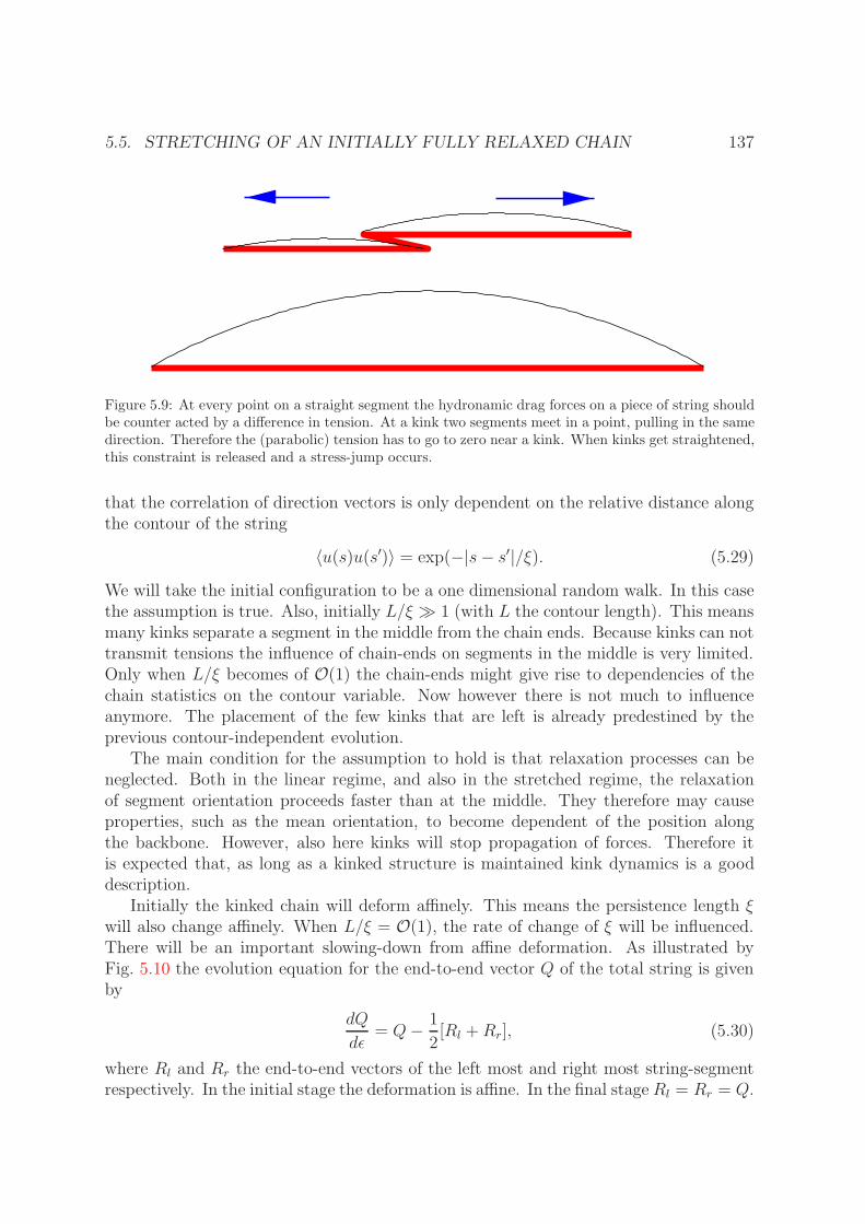
5.5. STRETCHING OF AN INITIALLY FULLY RELAXED CHAIN 137
Figure 5.9: At every point on a straight segment the hydronamic drag forces on a piece of string shouldbe counter acted by a difference in tension. At a kink two segments meet in a point, pulling in the samedirection. Therefore the (parabolic) tension has to go to zero near a kink. When kinks get straightened,this constraint is released and a stress-jump occurs.
that the correlation of direction vectors is only dependent on the relative distance alongthe contour of the string
〈u(s)u(s′)〉 = exp(−|s− s′|/ξ). (5.29)
We will take the initial configuration to be a one dimensional random walk. In this casethe assumption is true. Also, initially L/ξ 1 (with L the contour length). This meansmany kinks separate a segment in the middle from the chain ends. Because kinks can nottransmit tensions the influence of chain-ends on segments in the middle is very limited.Only when L/ξ becomes of O(1) the chain-ends might give rise to dependencies of thechain statistics on the contour variable. Now however there is not much to influenceanymore. The placement of the few kinks that are left is already predestined by theprevious contour-independent evolution.
The main condition for the assumption to hold is that relaxation processes can beneglected. Both in the linear regime, and also in the stretched regime, the relaxationof segment orientation proceeds faster than at the middle. They therefore may causeproperties, such as the mean orientation, to become dependent of the position alongthe backbone. However, also here kinks will stop propagation of forces. Therefore itis expected that, as long as a kinked structure is maintained kink dynamics is a gooddescription.
Initially the kinked chain will deform affinely. This means the persistence length ξwill also change affinely. When L/ξ = O(1), the rate of change of ξ will be influenced.There will be an important slowing-down from affine deformation. As illustrated byFig. 5.10 the evolution equation for the end-to-end vector Q of the total string is givenby
dQ
dε= Q− 1
2[Rl +Rr], (5.30)
where Rl and Rr the end-to-end vectors of the left most and right most string-segmentrespectively. In the initial stage the deformation is affine. In the final stage Rl = Rr = Q.

138 CHAPTER 5. BEAD-ROD CHAINS IN ELONGATIONAL FLOW
The length has attained its maximum value and the change in length thus stops. Thisformula will now be used to obtain a evolution equation for ξ. The starting point of thisderivation will be the change of 〈Q2〉
d
dε〈Q2〉 = 2[〈Q2〉 − 〈RQ〉], (5.31)
because of symmetry reasons the first and last segment can be treated on equal footing,we will use the symbol R. The evaluation of 〈Q2〉 in terms of ξ is most easy
〈Q2〉 =
∫ L
0
ds
∫ L
0
ds′〈u(s)u(s′)〉 = 2ξ2[exp(−L/ξ)− (1− L/ξ)]. (5.32)
The calculation of 〈RQ〉 is somewhat more complicated. To do the calculation somedefinitions of probabilities are needed. The most elementary one is that of p‖(s, s
′)this is the probability that the direction at position s equals that at position s′. Thisprobability can be easily obtained by noting that the product of the direction vectorsu(s)u(s′) has value one when they are parallel and minus one if they are directed inopposite directions
〈u(s)u(s′)〉 = p‖(s, s′)− [1− p‖(s, s
′)]. (5.33)
For points separated a small distance ∆s along the contour line
p‖(s, s+ ∆s).= exp(−1
2∆s/ξ). (5.34)
Using this probability the probability density for the lengths of R can be calculated. Itequals the probability that all tangent vectors up to position R are directed in the samedirections times the sign of the direction changes immediately thereafter in the interval[R,R+ ∆R].
p(R)∆R.=
(R/∆R)∑i
p‖(i∆R, (i+ 1)∆R)× [1− p‖(R,R+ ∆R)]
.=
[exp(−1
2∆R/ξ)
](R/∆R)
× [1− exp(−1
2∆R/ξ)]
.=
1
2ξexp(−1
2R/ξ)∆R
(5.35)
The last probability needed is the probability that R = L §
P (L) = lim∆R→0
[p‖(∆R)]L/∆R = exp(−1
2L/ξ). (5.36)
§Note that this derivation makes explicitly use from the fact that R is an end-segment.

5.5. STRETCHING OF AN INITIALLY FULLY RELAXED CHAIN 139
R2
Q 1
2(R1 +R2)
Q
R1
Figure 5.10: The velocity of a kink is the solvent velocity in the middle of this kink. The end-to-enddistance thus increases with the elongation rate times the distance of the midpoint of the first kink andthe midpoint of the last kink.
To compute 〈RQ〉, we write Q(s) as
Q(s) =
sR/|R| for s < |R|R +
∫ s
s′=|R| u(s′)ds′ for s > |R|. (5.37)
For a configuration where the first segment has length R, 〈u(R)u(R + dR)〉 = −1,therefore
〈RQ〉 =
∫ L
0
R[R−∫ L
R
〈u(R)u(s)〉ds]p(R)dR+ L2P (L)
= 6ξ2
[1− 1
3exp(−1
2L/ξ)(4 + L/ξ − exp(−1
2Lξ))
].
(5.38)
At this point we have expectation values that occur in Eq. (5.31) expressed in termsof ξ (and L). Inserting these expectation values in the formula therefore gives a equa-tion relating the persistence length ξ to the Hencky strain ε. This relation is mostconveniently expressed in the implicit form
ε(L/ξ) =
∫ L/ξ0
L/ξ
dx1
4x
(1− 12x)− (1 + 1
2x) exp(−x)
(1− 14x)− (1 + 1
4x) exp(−1
2x)
≈ log(√L/ξ0)− log(
√x∗)
+
∫ x∗
L/ξ
dx1
4x
(1− 12x)− (1 + 1
2x) exp(−x)
(1− 14x)− (1 + 1
4x) exp(−1
2x), x∗ 1,
(5.39)
which can be evaluated numerically. In this formula ξ0 is the persistence length of theinitial configuration. In the second form x∗ is any value much larger than 1 (but smalleror equal than L/ξ0). This form shows that the relation becomes invariant on the initialcondition if one uses a reduced Hencky strain ε − log(
√L/ξ0). This is not surprising.
The initial deformation of a randomly coil is
Q2 = 2ξ0L exp[2ε]. (5.40)

140 CHAPTER 5. BEAD-ROD CHAINS IN ELONGATIONAL FLOW
Thus the ratio of end-to-end length and the final length behaves as (Q/L) = exp[ε −0.5 log(L/ξ0)]. For a coiled state, the affine deformation stage takes a Hencky strain0.5 log(L/ξ0) − c, and only than the kink dynamics phase sets in. For the bead-rodchain in an elongational flow, one can distinguish the same two stages. Starting from athree dimensional random coil the deformation is first affine. During this phase the coilis squashed into an almost one dimensional structure. Then at a certain value of thereduced Hencky strain the kink dynamics mechanism takes over.
The expectation values for the end-to-end vector of the random coil is
〈Q¯Q¯〉 =
1
3Nδ
¯, (5.41)
where the number of rods N equals the final length: L = N . The end-to-end vector Q¯will initially deform affinely giving
〈Q¯Q¯〉 =
1
3N [exp(2ε)e
¯xe¯
x + exp(−ε)(e¯
ye¯
y + e¯
ze¯
z)]. (5.42)
Components of Q¯
in the compressive directions get rapidly smaller and in the elongateddirection they grow exponentially. After a few strain units we obtain a virtually onedimensional system with
〈Q2x〉 =
1
3N exp(2ε). (5.43)
Comparing this with Eq. (5.40) gives ξ0 = 16.
So far we have figured out the evolution of a kinked conformation, characterised by ξ,as function of the Hencky strain, and the initial value, ξ0, that should be used if the initialcoil is three dimensional. The remaining part needed, before a comparison between kinkdynamics and unfolding bead-rod chains can be made, is the computation of the stress.In the kink dynamics algorithm the stress is most easily calculated by adding up thecontributions of all individual segments. This is easy because one knows that the tensionin a segment is distributed quadratically (the contribution is 1
12εR3). But, because of the
finite length of the rope, it is not trivial to determine the distribution of segment lengthsin our semi-analytical approach. Therefore we use the Giesekus expression, Eq.(4.24).The quantity needed in this expression is the gyration tensor, G. When subtractingcentre-of-mass motion this becomes
G(x) =
∫ L
0
ds〈X(s)X(s)〉
=
∫ L
s=0
ds
∫ s
s′= 12
∫ s
s′= 12
〈u(s′)u(s′′)〉ds′ds′′
=
∫ L
0
ds
∫ s
0
ds′(L− s)s′
L〈u(s) u(s′)〉
= L3 exp(−x)− (1− x+ 12x2 − 1
6x3)
x4, x = L/ξ.
(5.44)

5.5. STRETCHING OF AN INITIALLY FULLY RELAXED CHAIN 141
kinks dynamics analyticallykinks dynamics simulation
We =1, N = 1024We =1, N = 128We = 467, N = 128We = 46:7, N = 128We = 4:67, N = 128
" 1
2log(N)
xx
=(m
ax
E
_")
6543210-1-2-3
1
0.1
0.01
0.001
0.0001
1e-05
1e-06
Figure 5.11: A Kramers chain in strong transient elongational flow. For large We a single curve existswhich relates the elongational viscosity to the strain. For chains with different lengths these curves canbe made to superimpose by assuming that on the onset of elongation the chain will deform affinely. Theresults superimpose perfectly with kink dynamics results (both simulated and solved semi-analytically).
Now the stress becomes
τxx = −1
2
[d
dt− 2ε
]G(x) = − ε
2
[− d
dε+ 2
]G(x)
=ε
2
[−(dε
dx
)−1d
dx+ 2
]G(x)
=ε
2L3
[−(dε
dx
)−1d
dx+ 2
]exp(−x)− (1− x+ 1
2x2 − 1
6x3)
x4
(5.45)
with x = L/ξ. Fig. 5.11 shows that the semi-analytical, the kink dynamics simulationsand the We =∞ simulations of the Kramers chain superimpose perfectly.
5.5.1 Elongation at moderate Weissenberg numbers
Fig. 5.12 shows the time evolution of a single Kramers chain for different Weissenbergnumbers. The initial condition is the same for all and also the random numbers usedare equal. The only difference is the elongation rate. The behaviour for large but finiteWeissenberg numbers can be understood qualitatively. In the We = ∞ case one canidentify segments in an unambiguous way. Because the tension at the kinks is zero, thetension distribution in a single segment will be very comparable to that of a chain ofthe same length of that segment (R). For the finite Weissenberg case for each segment

142 CHAPTER 5. BEAD-ROD CHAINS IN ELONGATIONAL FLOW
a segment-Weissenberg number can be defined as
WeR = 0.0285R2ε. (5.46)
Segments with a segment-Weissenberg number smaller than one will coil up. Segmentswith WeR > 1 will wrinkle up a bit but stay stretched as a whole. Because tension issmallest near the kinks the chain will be most wrinkled at those spots. Of coarse also thechain ends are almost tension free, which means they will coil up a certain amount. Forthe chain-Weissenberg number close to one the kink structure of the chain will becomeless and less. Empirically one finds that the kink dynamics mechanism breaks down atabout We = 10.
5.6 Remarks on the role of hydrodynamic interac-
tion
We have treated the three types of main chain conformations (coiled, stretched andkinked) and their dynamics. Before comparing the simulation with experiments we willremark on the influence of hydrodynamic interaction, which is not incorporated into thesimulations.
When the beads of a chain move affinely the beads do not generate an extra flowfield, and therefore there is no hydrodynamic interaction between beads. (The onlyperturbative flow field is caused by the finite size of the particle. The background velocitychanges over this length. This perturbation is negligible). Because of the constraints ofthe rods, the beads can not move freely and therefore there is hydrodynamic interaction.For strong flow, but still in the coiled state, forces transmitted through the backbone arenegligible compared to the viscous drag on the bead. Beads separated a few Kuhn stepsfrom each other do effectively not feel each other. They separate affinely. Hydrodynamicinteraction is now a localised effect. The conclusion therefore is: in strong flow the coilinitially deforms affinely, hydrodynamic interaction can not change this.
When the coil is deformed by elongational flow a one dimensional structure consistingof stretched segments is formed. The beads in these segments can not move affinely withrespect to each other. Therefore hydrodynamic interaction will be important. In twopapers [21] and [22] Batchelor treats the (drag)force distribution along a slender body.In a first approximation (in the small ratio of width and length) the drag force per unitlength for a rigid slender body in elongational flow is
Fdrag(x) =2π
log(L/b∗)ηsεx, (5.47)
where L is the length of the body, and b∗ its radius. The important thing to note isthat the drag force remains linear in the position along the contour. The linearity ofthe drag force makes that the kink dynamics mechanism still remains the same. Asegment will move with the background fluid velocity at the mid-point of that segment.The conclusion is that hydrodynamic interaction is probably of minor influence on the

5.6. REMARKS ON THE ROLE OF HYDRODYNAMIC INTERACTION 143
" = 4:50
" = 3:64
" = 2:79
" = 1:93
" = 1:07
" = 0:21
" = 0
" = 5:36
2:5 15:0 10 20 80 320We:
Figure 5.12: Kramers chains in strong flow, at different Weissenberg numbers. The same initial con-ditions, and realisations of the random process were used. The lower We the more short segments getcoiled up. The more segments are coiled up, the more diffuse the kinks dynamics picture becomes. Itbreaks down at about We = 10.

144 CHAPTER 5. BEAD-ROD CHAINS IN ELONGATIONAL FLOW
unravelling mechanism. Of course, the unravelling polymer is not a rigid slender body,but the individual segments are. Neighbouring segments may influence each other.
Although the unravelling mechanism is not influenced by hydrodynamic interaction,the stress is. Computing the elongational stress for the stretched case gives
τxx = n
∫ 12L
− 12L
xF (x)dx =π
6 log(L/b∗)nηsεL
3, (5.48)
where n is the number of polymers per unit volume. For b∗ one can take the Kuhnstep (now L/b∗ = N). This is probably be not completely correct, but because of thelogarithm it will only give a small error. The stress of a fully stretched chain in strongflow is expected to increase a bit more slowly as function of molecular weight. Not asM3 but as M3/ logM (M is proportional to L).
In ref. [22] Batchelor makes a very interesting remark. The stress expression Eq. (5.48)is only valid in the limit that
nL3 log(L/b∗) 1. (5.49)
Substituting this inequality into Eq. (5.48) gives that the stress expression is only validwhen the polymer contribution is smaller than the solvent contribution! In experimentsone measures polymer contributions that are typically a factor 104 as large as the solventcontribution. This means these fluids can not be considered dilute, but are semi-dilute.When separated less than the stretched length L hydrodynamic interaction betweenneighbours is significant for the stress expression. In this case
τxx ≈ n
∫ 12L
− 12L
xF (x)dx =π
−3 log(nb∗ 2L)nηsεL
3. (5.50)
We assume that, even in this regime, the neighbour-neighbour interaction of polymersstill does not significantly influence the unravelling dynamics.
The conclusion is that in strong flow hydrodynamic interaction does not significantlyinfluence the dynamics. The stress, however, is affected.
On the other hand, when non-affine motion is important, hydrodynamic interactionwill severely influence the evolution of the polymer conformation. Therefore one ex-pects to see large differences between the freely draining simulations and experiments(or simulations including hydrodynamic interaction) for stationary conformations, forchain relaxation and for small Weissenberg number dynamics. These differences willbe qualitative. For example in the coiled state, the main characteristic, namely thatof a spectrum of relaxation times is still valid. The form of the relaxation spectrumis different. For the freely draining case the spectrum is the Rouse spectrum. Whenhydrodynamic interaction is included the so-called Zimm spectrum is more appropriate.
For the stretched state the main characteristic is that there is no characteristic timescale. The relaxation occurs via a power law. In the freely draining case we found thispower law is t−0.5 for the stress. When including hydrodynamic interaction the dragchanges with conformation, still there is not a reason to suspect a characteristic time.Therefore a power-law dependence is still to be expected (see Fig. 5.15).

5.7. A COMPARISON WITH EXPERIMENT 145
5.7 A comparison with experiment
In this section we will discuss some experimental findings for linear flexible polymerchains in elongational flow. Only recently high quality elongational data became avail-able for dilute polymer solutions in elongational flow. The two techniques that wereused for producing this data are the study of individual DNA molecules in elongationalflow by fluorescence microscopy and filament stretching of a drop of dilute polymersolution. Much of the experimental data can not be explained by commonly used con-stitutive equations. The kink dynamics picture, however, gives a qualitative explanationand sometimes even a quantitative one. But the data also poses some doubts on thecompleteness of this picture.
5.7.1 Stretching individual DNA molecules
In a long series of papers [23, 24, 25, 26, 27, 28, 29, 30] the group of Chu et al. havepublished the results of a ‘micro-rheological’ experimental technique. By means of videofluorescence microscopy they are able to look at the dynamics of a single DNA molecule.The resolution of this technique is approximately 1µm, which is enough to partiallyresolve a DNA molecule (22− 84µm). (However, the Kuhn step of a DNA molecule isO(0.1µm), which is significantly below the resolution). Not only can they measure thedynamics, they are also able to influence it. By optical trapping of a 1µm polystyrenesphere attached to the end of a DNA molecule it can be moved around. A secondtechnique is the use of equipment that can create (ideal) micro flow fields.
For our purposes the most interesting paper in the series is Smith and Chu [29](which contains an important improvement on results presented in [27]). In this paperDNA molecules in sudden planar elongational flow are monitored. The flow cell is across-slot apparatus. First a DNA coil is manipulated into the stagnation point. Then,when the coil is re-equilibrated, the flow is very rapidly turned on. The Weissenbergnumber is as high as O(100), which is well into the kink dynamics regime.
When looking at individual DNA-molecules stretching in this strong flow one observesa large spread in the unravelling process. Some chains deform almost affinely whereasothers get folded in half and the unravelling comes almost to a halt. How a coil willunravel is largely a matter of chance. A determining factor is the location of the end-points with respect to each other and to the centre of mass of the chain. The formationof the structures is mostly determined in the first two strain units, where the coil issqueezed. For example, if subsequent to this compression the chain ends are near toeach other the possibility that the coil will evolve into a double folded structure is high.In Perkins et al. [27] the authors categorised the squashed coils as dumbbell (middlestretched chain-ends coiled), half dumbbell (one end coiled), kinked (ends stretched, coilin the middle) folded (into two large segments) and coiled. The first evolves quickestto the stretched state, the last slowest. That folded structures deviate most from affinedeformation can be easily understood in terms of the analytic kink dynamics equationEq. (5.30).
Larson and Hu [17] performed an extensive numerical analysis of the experiments by
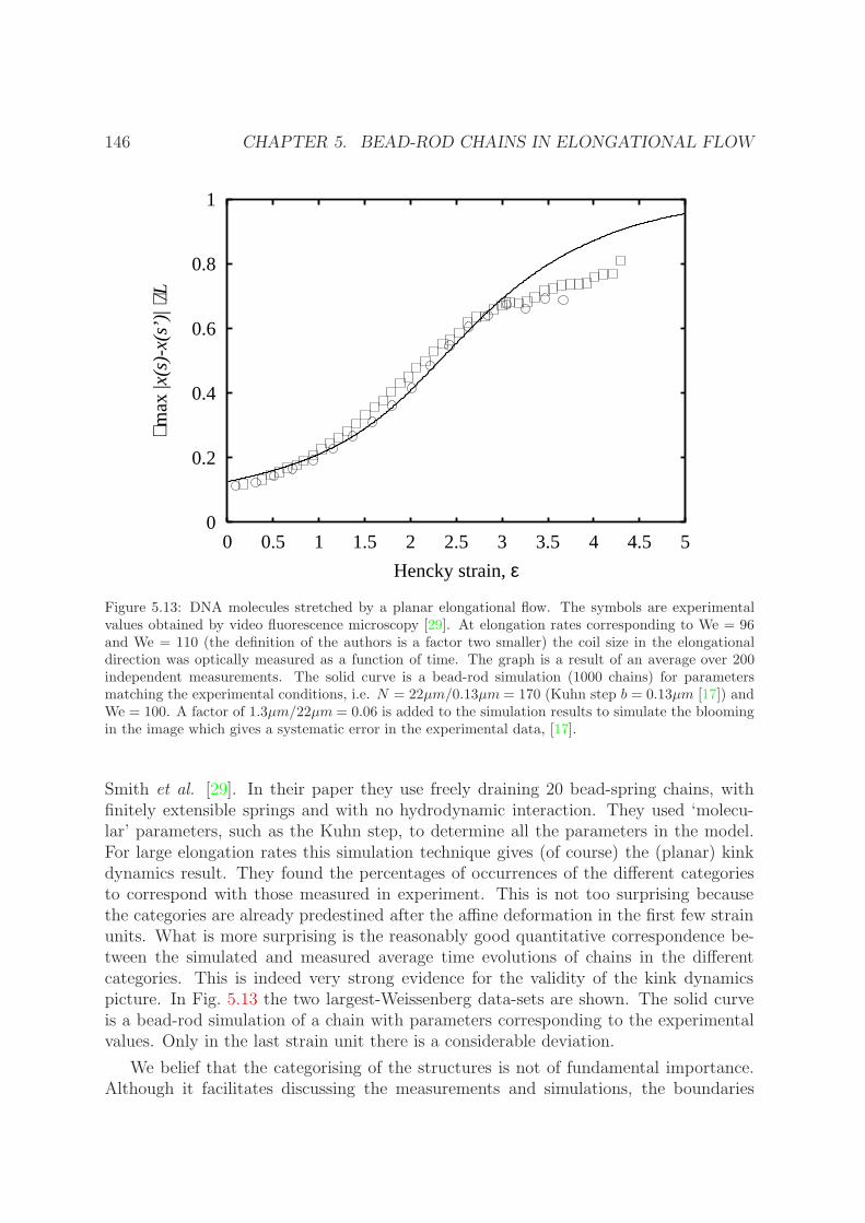
146 CHAPTER 5. BEAD-ROD CHAINS IN ELONGATIONAL FLOW
0
0.2
0.4
0.6
0.8
1
0 0.5 1 1.5 2 2.5 3 3.5 4 4.5 5
⟨ max
|x(s
)-x(
s’)|
⟩/L
Hencky strain, ε
Figure 5.13: DNA molecules stretched by a planar elongational flow. The symbols are experimentalvalues obtained by video fluorescence microscopy [29]. At elongation rates corresponding to We = 96and We = 110 (the definition of the authors is a factor two smaller) the coil size in the elongationaldirection was optically measured as a function of time. The graph is a result of an average over 200independent measurements. The solid curve is a bead-rod simulation (1000 chains) for parametersmatching the experimental conditions, i.e. N = 22µm/0.13µm = 170 (Kuhn step b = 0.13µm [17]) andWe = 100. A factor of 1.3µm/22µm = 0.06 is added to the simulation results to simulate the bloomingin the image which gives a systematic error in the experimental data, [17].
Smith et al. [29]. In their paper they use freely draining 20 bead-spring chains, withfinitely extensible springs and with no hydrodynamic interaction. They used ‘molecu-lar’ parameters, such as the Kuhn step, to determine all the parameters in the model.For large elongation rates this simulation technique gives (of course) the (planar) kinkdynamics result. They found the percentages of occurrences of the different categoriesto correspond with those measured in experiment. This is not too surprising becausethe categories are already predestined after the affine deformation in the first few strainunits. What is more surprising is the reasonably good quantitative correspondence be-tween the simulated and measured average time evolutions of chains in the differentcategories. This is indeed very strong evidence for the validity of the kink dynamicspicture. In Fig. 5.13 the two largest-Weissenberg data-sets are shown. The solid curveis a bead-rod simulation of a chain with parameters corresponding to the experimentalvalues. Only in the last strain unit there is a considerable deviation.
We belief that the categorising of the structures is not of fundamental importance.Although it facilitates discussing the measurements and simulations, the boundaries

5.7. A COMPARISON WITH EXPERIMENT 147
between the categories are vague. The underlying thought for introducing them mightbe that the wide spread in evolution of the structures necessitates different treatmentof the different categories when trying to model the unravelling process. However, kinkdynamics does automatically generate these structures. Our semi-analytical approachdoes also capture this phenomena. The wide spread in unfolding rates of the differentcategories is well modelled in the semi-analytic kink dynamics theory which only uses oneparameter, namely ξ. This means one does not explicitly have to make the categorisationto describe the unfolding process well.
Here we only discussed the DNA experiments that looked at the unravelling processin strong elongational flow. In other papers of the same group e.g. the relaxation of aninitially stretched chain [24], the stationary extension of a chain kept fixed at one endin a uniform flow [26] and the dynamics of a chain kept fixed at both its end-points [28],were studied. In these flows hydrodynamic interaction is important. Because this effectis not included in our simulation a comparison of the simulations with these experimentsdoes not make much sense. In Larson at al. [31] it is shown that the stationary measure-ments of [26] are described very well by a dumbbell model that includes hydrodynamicinteraction.
Furthermore one of the most interesting aspects of relaxation subsequent to strongelongation is the rapid relaxation described in §5.4. In this initial regime the largest partof the stress relaxes, but the chain remains almost stretched. This process is difficult toanalyse using a blurred optical technique.
5.7.2 Filament stretching rheometry
Probably the best way to measure elongational properties of dilute polymer solutions isthe filament stretching technique introduced by Sridhar et al. [32]. Two disks with adroplet of polymeric liquid in between are separated quickly. Hencky strains of 7 canbe achieved this way. The force on the upper disk is measured. Because the rate ofelongation depends on the position in the filament the waist, i.e. the diameter in themiddle of the filament, is measured. At the waist the deformation is purely elongational.From the rate of change of the diameter one can deduce the elongation rate in the middle.Because inertial effects are negligible, the force transmitted through the waist can bededuced from the measured force on the disk. In this way both the elongation rate andthe elongational stress in the waist are simultaneously measured. By using a feedbackloop one can impose any elongation history. Several groups have developed a similarfilament stretching device [32, 33, 34].
The most important finding of the filament stretching measurements is that, at largeenough Weissenberg number, the elongational stress scales viscously, i.e. when the elon-gation rate is doubled, the stress doubles. This is indeed predicted by kink dynamicsand found in the bead-rod simulations. One of the nicest illustrations of this scaling isdepicted in Fig. 5.14.
Attempts to fit experiments to constitutive equations failed miserably [36]. Thereason is that the common constitutive equations and simple dumbbell models behaveelastically. As pointed out in §5.5 internal structure and, as in the case of the FENE

148 CHAPTER 5. BEAD-ROD CHAINS IN ELONGATIONAL FLOW
Figure 5.14: Viscous scaling of the elongational stress as function of Hencky strain in strong uniaxialelongational flow, reproduced from [11]. At different strains the elongation rate is stepped up or down.The elongational viscosity is not influenced.

5.7. A COMPARISON WITH EXPERIMENT 149
0
10000
20000
30000
40000
50000
60000
70000
0 0.1 0.2 0.3 0.4 0.5 0.6 0.7 0.8 0.9 1 1.1
elon
gatio
nal s
tres
s, τ
xx-
τ yy
[Pa]
time, t [s]
8234 (t-0.036) -0.91
Figure 5.15: The relaxation subsequent to a strong elongation of ε = 6 of different elongation rates(form [35]). The relaxation curve is independent of the previous elongation rate. The curve fits well toa power law with exponent −0.91. Extrapolating the time to zero one finds an initial stress of the rightorder of magnitude (105 − 106) Pa.
150 CHAPTER 5. BEAD-ROD CHAINS IN ELONGATIONAL FLOW
dumbbell the distribution of orientations in an ensemble, can give rise to viscous scaling.As in this case of the FENE-dumbbell, the stresses do not have to be viscous. Otherphenomena that give rise to viscous scaling are dissipative effects, such as internal vis-cosity. These phenomena give rise to a viscous part in the stress. We will discuss theissue of viscous and dissipative stresses in §5.8.
Experimentally much effort has been made to identify viscous stresses. In Orr etal. [35] a procedure to identify possible viscous stresses is introduced. They look at therelaxation of the stress after sudden cessation of elongational flow. The initial relaxationis faster than the force transducers can measure. They postulate that that part of thestress is viscous, i.e. relaxes instantaneously. To determine the viscous stress they fitthe relaxation curve to a sum of two decaying exponentials. They take the differencebetween the fit, extrapolated to the point the flow is stopped, and the stress, just beforethe flow is stopped, to be the viscous part of the stress. As will be discussed in §5.8in bead-rod chain simulations the viscous stress is very small. In this setting, afterthe cessation of flow, a stretched chain (or if not fully stretched, a stretched chainsegment) relaxes via the theory described in §5.4. After a strong deformation, with acertain strain, the conformation of a chain is almost independent of the elongation rate.The tension in stretched segments will differ a bit, but this difference relaxes almostinstantaneously after cessation of flow. After this rapid initial relaxation process thecurves of stress versus time will superimpose independently of the previously appliedstrain rate. According to Eq. (5.22) the curve will behave as a inverse square rootof time. In Fig. 5.15 two relaxation curves from [35, Fig. 7] are plotted. They weremeasured subsequent to strong elongation of Hencky strain ε = 6, but with differentstrain rates. It is shown that the two sets indeed superimpose, and fit very well to apower law. If one extrapolates the fitted curve to t = 0, one even finds a stress of thesame order of the stress before relaxation. There seems no need to introduce a viscousstress. The power is however not −0.5, but −0.91. We postulate that this differencewith the relaxation of a free draining bead-rod chain as presented in §5.4 is caused byhydrodynamic interaction.
In [33] and [37] stress growth in strong elongation and the subsequent relaxationfor different strain rates were reported. The authors plotted the relaxation curves inthe same graph as the extensional data. For the relaxation part εt was plotted onthe strain axis. Also the elongational stress was scaled by the final elongation rate εt.The relaxation curves almost superimpose. This is well explained by the fact that theexponent of relaxation −0.91 is near to −1, because η+
E ≈ τxx/ε ∝ 1/(tε).
Li and Larson [18] analysed the filament stretching data presented in [11] and [19]using exactly the same method as in the analysis of DNA data in [17]. The viscous scalingfor different strain rates is confirmed. In the paper of Gupta et al. [19] extensional datausing polymer solutions of different molecular weights are presented. Li and Larsonfound that these data series superimpose if the Trouton ration is divided by M2 andthe Hencky strain is not changed. This scaling is not at all in accordance with thatgiven by kink dynamics. Therefore it is not surprising that (especially for the largemolecular weights) experiment and simulation do not superimpose. In Fig.5.16 we plot

5.7. A COMPARISON WITH EXPERIMENT 151
0.0001
0.001
0.01
0.1
1
-5 -4 -3 -2 -1 0 1 2 3
η E/(
-π/3
ηs
n b3 N
3 / lo
g(n
b3 N))
Hencky strain, ε-0.5 log N
N=5253
N=13470
N=26938
Figure 5.16: Unravelling of long chains in strong uniaxial elongation (data from [19], N is the number ofKuhn steps). For these long chains quantitative agreement between kink dynamics and measurementsis poor.

152 CHAPTER 5. BEAD-ROD CHAINS IN ELONGATIONAL FLOW
the experimental data using the scaling suggested by kink dynamics. To rescale thestress we have used the Batchelor expression for the maximum stress Eq. (5.50). Thisis not perfect, but at least the measurements do not exceed the theoretical maximumstress and data is no longer order of magnitudes off. The longer the chains the largerthe deviation from the maximum stress value.
We thus see in Fig. 5.13 a good comparison between theory and measurements forshort chains and in Fig. 5.16 a rather bad agreement for much longer chains. An ob-vious suggestion is that, for long chains, there is an extra mechanism that slows theunravelling of the chain considerably. A candidate for such a mechanism is that ofself-entanglements. The chain is entangled with another part of the same chain. Be-fore the chain can fully stretch it has to disentangle. If the disentangling mechanismis much slower than the unravelling of kinks, first the segments between entanglementswill unkink, and then a kind of plateau is reached.
5.8 Viscous and dissipative stresses
Already in §5.5 we found that the unravelling in strong flow gives rise to viscous scaling.This means that the stress is proportional to the elongation rate. This finding, which isnot explained by most traditional constitutive equations, is confirmed by experiments.Many authors have suggested that an important part of this viscous scaling is caused byviscous stress, see e.g. [35, 37]. Viscous stress is defined as the part of the total stressthat is proportional to the instantaneous elongation rate. To distinguish elastic stressthat adapts very quickly from viscous stress one can reverse the flow. Then viscous stressstress will change sign, but elastic stress will not. In this section we will first show thatviscous stresses are irrelevant in the bead-rod chain simulations, then we will discuss themechanism behind the appearance of the viscous scaling.
In Fig. 5.17 the stress in a stationary elongational flow is shown. The differencebetween the perturbed coil regime, We < 1, that can be described by Rouse theoryand the stretched chain, We > 1 is very clear. As discussed in §4.5.2 the stress of aKramers chain can be decomposed into several contributions. Three contributions canbe discriminated, see Eq. (4.25), namely an elastic contribution, a material momentumflux contribution and a viscous contribution. By definition the viscous contributiondisappears instantaneously when the flow is stopped. The other contributions have finiterelaxation times. The elastic stress and the momentum flux are functions of the polymerconfiguration. The viscous stress has a linear dependence on the rate of deformationtensor. The multiplication factor, which is a fourth order tensor, is again a function ofconformation only. In Fig. 5.18 the three partial stresses are plotted for an ensemble ofbead-rod chains of length 32 and 128.
In §5.3, Eq.(5.11), we showed that in the coiled regime, the viscous stress is negligi-ble. In the stretched state the total stress becomes O(N3ε). The material momentumcontribution (i.e. the contribution due to momentum exchange connected to particleexchange) is of O(N) and thus negligible. For a stretched chain, we can expand thetheory for relaxation of a chain, presented in §5.4. Now a hydrodynamic drag term has

5.8. VISCOUS AND DISSIPATIVE STRESSES 153
2R1
0G(1s) exp(2Wes)ds
128 rods32 rods
We
x
x
/We
1010.1
1000
100
10
1
128 rods32 rods
dumbbell model
We
x
x
= E(max)_"
1010.1
10
1
0.1
0.01
Figure 5.17: The scaled elongational viscosity of an ensemble of Kramers chains as function of theWeissenberg number in a stationary uniaxial elongational flow. The first graph shows the appropriatescaling for the near equilibrium regime We < 1. It is well described by the Rouse chain results. The lineis the 32-rod result for the Rouse chain. The second graph shows appropriate scaling for the stretchedstate. The 32-rods result is compared with a dumbbell model. This dumbbell model will be describedin appendix 5.A.

154 CHAPTER 5. BEAD-ROD CHAINS IN ELONGATIONAL FLOW
128 rods32 rods
We
xx
;elast=N
1010.1
10
1
0.1
128 rods32 rods
We
xx
;m
om
=N
1010.1
10
1
0.1
128 rods32 rods
We
xx
;visc=N_"
1010.1
10
1
0.1
Figure 5.18: The three contributions to the stationary stress normalised in such a way that the resultinggraphs only have a We-dependence. Note that for the viscous part, not the stress but the viscosity isplotted. The different contributions are conformation dependent. For We < 1 the conformation isthat of a perturbed coil. The stress contributions are perturbations on the equilibrium coil value. ForWe > 1 the chain is stretched. The stress becomes very sensitive to the degree of stretching.

5.8. VISCOUS AND DISSIPATIVE STRESSES 155
to be added to the force balance in the stream-wise direction, Eq. (5.12),
∂
∂t〈y2〉 .= −2
∂2
∂s2T − 2ε. (5.51)
For the stationary situation this causes the tension in the chain to have a parabolicdependence on position s. The stationary elongational viscosity will be
τxx =1
12N3ε. (5.52)
It is very instructive to rewrite the set of equations Eq. (5.51) and Eq. (5.15) as
∂
∂t〈y2〉+ 4〈y2〉T = 8,
∂2
∂s2T − 2〈y2〉T = −(4 + ε), T (0) = T (N) = 0.
(5.53)
The first equation denotes the time evolution of the conformation. The second one isthe computation of the tension. This is not an evolution equation, but an instantaneousone. On the left-hand side the expression is linear in the tension T . The viscous stressis the part that depends linearly on ε. Putting ε = 0 gives the elastic stress. The ratioof the two stresses is
τxx,visc
τxx,elast=ε
4. (5.54)
(This is valid even in transient situations). In Fig. 5.19 we show a comparison of elasticand viscous stresses obtained from stationary bead-rod simulations. Indeed the relationbetween viscous and elastic stress is confirmed. With the use of Eq. (5.52), one finds forthe stationary stresses:
τxx,elast =εN3
12 + 3ε
τxx,visc =ε2N3
48 + 12ε.
(5.55)
Viscous stresses only become important when the Peclet number, Pe, is of order oneor larger (in the dimensionless form ε = O(1)). The viscous stresses are caused by theinextensibility of the rods, it becomes dominant when flow is strong on the scale of therods. For realistic elongational flows of long flexible chains the Weissenberg number, We,can be quite large, but Pe 1. Viscous stresses are thus of no practical importance.This point is also stressed by Doyle et al. [13, 15].
Combining the facts that in a strong elongational flow, the transient stress scalesviscously, i.e. linearly with the elongation rate, (also when Pe 1) and that the viscousstress is of no importance poses a conceptual problem. In early investigations [4], [7]this problem was not recognised. Because of the fact that the Brownian motion is of no

156 CHAPTER 5. BEAD-ROD CHAINS IN ELONGATIONAL FLOW
128 rods32 rods
viscous stress
elastic stress
_"
stresses
totalstress
1010.1
1
0.8
0.6
0.4
0.2
0
_"=4128 rods32 rods
_"
xx
;visc= xx;elast
109876543210
2.5
2
1.5
1
0.5
0
Figure 5.19: The viscous stress and the elastic stress in stationary elongational flow as function of theelongation rate. For Pe 1 the elastic stress is dominant.

5.8. VISCOUS AND DISSIPATIVE STRESSES 157
importance to the dynamics of unravelling process, Brownian motion was not taken intoaccount in these simulations. In this limit (Pe = ∞) there are no relaxation processesand all stress is viscous.
Relating the viscous scaling to viscous stress only is a mistake. Therefore the termdissipative stress [14] might be better. This is however a difficult concept. In oscillatoryrheology one has the concepts of the loss and the storage modulus, see Eq. (5.1). Thestress corresponding to the loss modulus is in phase with the shear rate, energy isdissipated, this stress can be categorised as dissipative. The storage modulus is relatedto the internal free energy (in the case of an ensemble of Kramers chains, entropy).
When rapidly deforming a linear elastic dumbbell and then reversing the deformationthe stress as a function of strain will behave the same when going forth and back.The work done to perform the initial deformation is totally recovered upon reversalof the deformation. This stress can be labelled as ‘recoverable stress’. When doingthe same experiment for a (non-Brownian) rod the stress will reverse sign. The sameamount of work will be done when going back. The stress can not be recovered, it hasa dissipative character. A third experiment is that of two beads connected by a string.When separating the beads so far that the string becomes stretched, a stress will arise.When reversing the flow the tension in the string will instantaneously disappear, thestress is thus dissipative. These examples are directly related to the elastic or viscousnature of the stresses. The dissipative nature of the stress in the last example canhowever also be interpreted in a second way.
In a constant flow field, when the conformation of an ensemble of dumbbells orchains becomes stationary, the stress becomes dissipative. The dissipative nature hasnothing to do with the fact the stress is elastic or not. As already discussed in §5.5,when strongly elongating an ensemble of FENE springs part of the ensemble, namelythe part that has reached the maximum length, becomes stationary and gives rise toa dissipative stress. This stress contribution dominates the contribution of the not yetfully extended springs. When strongly stretching a chain, the conformations of the rodsin the stretched segments are quasi stationary. Their conformation is stretched. Onlywhen a kink passes by they will flip orientation. After this, their contribution to thestress will again be quasi stationary.
The fact that (quasi) stationary or dissipative stress scales viscously might seemstrange. One might think: the stress is dominantly elastic, therefore it does dependon the conformation only, and the conformation of e.g. a kinked chain is only straindependent. This is not true. Increasing the strain rate does change the configuration,but only very slightly. This slight change has major consequences. A FENE spring hasa diverging force law at maximum extension. The tension in a bead-rod chain segmentdiverges as T = 2/〈y2〉. In (quasi)stationary structures the tension has to balance dragforces. This means the stress is proportional to the elongation rate.
In Fig. 5.20 we have plotted an elongational straining followed by a flow reversalat two Hencky strains (ε = 3 and ε = 6). The total Hencky strain is zero after onecycle. Subsequent to the first few strain units, a kinked structure will be formed. Fromthen on the stress scales viscously. When reversing the flow, the stretched segments
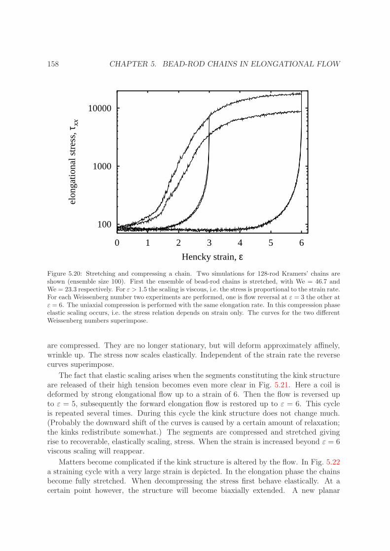
158 CHAPTER 5. BEAD-ROD CHAINS IN ELONGATIONAL FLOW
100
1000
10000
0 1 2 3 4 5 6
elon
gatio
nal s
tres
s, τ
xx
Hencky strain, ε
Figure 5.20: Stretching and compressing a chain. Two simulations for 128-rod Kramers’ chains areshown (ensemble size 100). First the ensemble of bead-rod chains is stretched, with We = 46.7 andWe = 23.3 respectively. For ε > 1.5 the scaling is viscous, i.e. the stress is proportional to the strain rate.For each Weissenberg number two experiments are performed, one is flow reversal at ε = 3 the other atε = 6. The uniaxial compression is performed with the same elongation rate. In this compression phaseelastic scaling occurs, i.e. the stress relation depends on strain only. The curves for the two differentWeissenberg numbers superimpose.
are compressed. They are no longer stationary, but will deform approximately affinely,wrinkle up. The stress now scales elastically. Independent of the strain rate the reversecurves superimpose.
The fact that elastic scaling arises when the segments constituting the kink structureare released of their high tension becomes even more clear in Fig. 5.21. Here a coil isdeformed by strong elongational flow up to a strain of 6. Then the flow is reversed upto ε = 5, subsequently the forward elongation flow is restored up to ε = 6. This cycleis repeated several times. During this cycle the kink structure does not change much.(Probably the downward shift of the curves is caused by a certain amount of relaxation;the kinks redistribute somewhat.) The segments are compressed and stretched givingrise to recoverable, elastically scaling, stress. When the strain is increased beyond ε = 6viscous scaling will reappear.
Matters become complicated if the kink structure is altered by the flow. In Fig. 5.22a straining cycle with a very large strain is depicted. In the elongation phase the chainsbecome fully stretched. When decompressing the stress first behave elastically. At acertain point however, the structure will become biaxially extended. A new planar

5.9. COARSE GRAINING A BEAD-ROD CHAIN 159
100
1000
10000
4.6 4.8 5 5.2 5.4 5.6 5.8 6 6.2
elon
gatio
nal s
tres
s, τ
xx
Hencky strain, ε
Figure 5.21: A cycle of uniaxial compression and uniaxial elongation between ε = 6 and ε = 5 is ranthrough several times (for a 1000 128 bead-rod ensemble at We = 46.7). The stress scales elastically.
kinked structure will form and the scaling becomes viscous again.
5.9 Coarse graining a bead-rod chain
An important application for constitutive equations is their use in macroscopic flowsimulations. Bead-rod chains are computationally too expensive to use in complex flowsimulations. A less-detailed, more coarse-grained description would therefore be wel-comed.
The mental picture we have sketched in the preceding sections is that of three basicchain conformations: the coiled state, the stretched state and the kinked state, all withtheir own particular dynamics. In this section we will discuss the possibility to coarsegrain the bead-rod chain to a simple model which is capable of describing the all threestates.
The basic feature of the coiled state is that of a spectrum of relaxation times. Linearrheological theory describes this near-to-equilibrium state. The stress can be expressedas a single integral over the deformation history, which is characterised by the rate-of-deformation tensor. The full relaxation spectrum is captured in the relaxation modulus.
Stationary stress and relaxation from the stretched stage is well described by a dumb-bell model. As remarked before, in these cases the conformation of a chain will samplemany microstates, and a thermodynamic treatment introducing less degrees of freedom

160 CHAPTER 5. BEAD-ROD CHAINS IN ELONGATIONAL FLOW
-5000
0
5000
10000
15000
20000
0 2 4 6 8 10 12
elon
gatio
nal s
tres
s di
ffer
ence
, τxx
-τyy
Hencky strain, ε
Figure 5.22: A cycle of strong uniaxial elongation and compression with large strains, for two Weis-senberg numbers We = 46.7 and We = 23.3. Starting from a coil chains will stretch. In the compressionphase, first the chain is compressed into a wrinkled conformation. Here the scaling will be elastically.Uniaxially compressing the chain further the structure will be biaxially extended. Now a new planarkinked structure is created. This is the initial configuration for the new cycle.

5.9. COARSE GRAINING A BEAD-ROD CHAIN 161
is useful. In appendix 5.A we describe a method to coarse grain a bead-rod chain toa dumbbell model. It is shown that the relaxation of a bead-rod chain is indeed welldescribed by this dumbbell model. Dumbbell models only represent the linear regimein a crude way. They have a single relaxation time and therefore can only describe theslowest mode.
Combining the spectrum of relaxation time of the linear regime, with the nonlinearbehaviour of the dumbbell theory is difficult. A common procedure is to use multimodemodels. A linear superposition of a dumbbell (or other thermodynamicly coarse grainedsystems) with different parameters is used. The superposition gives a representationof the spectrum of relaxation times. The individual dumbbells represent nonlinear be-haviour. This combination of two regimes is more a fitting procedure than a procedurefounded on a physical picture.
When one also wants to capture the third basic conformation of a bead-rod chain,the kinked state, in a coarse-grained model an extra complication is added. Thereis however a good indication that an approximate description might be found. Thisindication is that kink dynamics can be described well by only one parameter (ξ, see§5.5). Both from experiment and from simulation, the same mental picture emerges. Instrong flow, a kinked structure is created. This structure has its own dynamics. Thisdynamics is governed by kink dynamics. (For longer chains other dynamics e.g. that ofself-entanglements might be dominant.)
Kinks are tension free. This causes the motion of the segments in between kinksto be to be almost mutually decoupled. Because segments are decoupled segments cannot influence each other. For example during relaxation the large features of the kinkstructure is not influenced. Because the kinks are tension free they do not transmitperturbations. The long lengthscales will not relax. The kink structure is meta-stable.This is why a thermodynamic treatment of the whole chain does not work. Individualsegments can sample many micro-states, but the chain as a whole remains in the samekinked state.
This is nicely illustrated in Fig. 5.23. Here at Hencky strain ε = 3 the flow isturned off for a moment. The segments relax. They do however not influence the kinkedstructure. As discussed in §5.5.1 pieces of chain near the kinks will become more coiled.That is all. The end-to-end distance of the full chain is almost not influenced. When theflow is turned on again, the kinked structure proceeds to evolve at the point where it wasstopped. This becomes clear as the segments become fully stretched again. Then thestress will scale viscously again, and the strain-stress evolution goes on as if no relaxationprocess occurred. This behaviour is also found in experiments [11]. A remarkable resultin Fig. 5.23 is that even for quite long relaxation times such as 0.2τ1, the kink structureseems to be unaffected.
In the flow reversal experiments discussed in the previous section there is a similarsituation. The strong elongation gives rise to the creation of the kinked conformation.When reversing the flow, the individual segments are compressed. Only when reversingthe flow again, and elongating the segments such that they become stretched again, thekinked structure evolves further. Only stretching beyond the maximum Hencky strain

162 CHAPTER 5. BEAD-ROD CHAINS IN ELONGATIONAL FLOW
0
2000
4000
6000
8000
10000
12000
14000
16000
2.5 3 3.5 4 4.5
elon
gatio
nal s
tres
s, τ
xx
Hencky strain, ε
0.0005 τ10.005 τ10.05 τ1
0.2 τ1
Figure 5.23: Restart of strong elongational subsequent to relaxation of a certain time. When segmentsare stretched again the strain-stress relation will follow the original curve. This indicates that, even forrelatively long pauses, the kink structure is not affected.

5.10. CONCLUSIONS 163
influences the kink structure.Deriving a coarse-grained model for the bead-rod chain in strong uniaxial elongational
flow including (not too long) instances of relaxation and flow reversal should not betoo difficult. The kink structure is a function of max(ε). The segments behave as anensemble of independent FENE-chains, described in §5.A. What the ensemble looks likeis dominated by the kink dynamics (and probably self-entanglement dynamics). Thissuggestion shows many resemblances to work of Ghosh et al. [38]. For strong flow, theFENE-character becomes only clear when the segments are not extended, i.e. ε < max(ε)or ε = 0. Also for elongation at moderate Weissenberg the FENE-character of thesegments will play an important role. To accurately describe experiments one should alsosomehow include hydrodynamic interaction into the FENE-dumbbell evolution equation.
The situation becomes very much more complicated when the kink structure can relaxor is deformed by more complicated deformation histories. In the near coil regime thereis no decoupling of kink structure and segments. In the coiled regime there is muchcommunication between beads along the backbone. A whole spectrum of relaxationtimes has to be taken into account. A single FENE dumbbell can not capture thisspectrum. Furthermore, hydrodynamic interaction will be important. The crossoverbetween the dynamics of the kinked state and the coiled state is troublesome. Althoughwe saw in Fig. 5.23 that the kink structure stays fully intact for times as long as 0.2τ1,it should break down at times O(τ1). When deformation is restarted the kink structurehas to be re-established. How to describe the break down of the kink structure is notclear. Somehow a crossover from the kinked configuration to the coiled configurationneeds to be established.
The kink structure in uniaxial elongational flow is described by the theory presentedin §5.5. How to describe the kink structure in e.g. biaxial elongation is more difficult.The structure will not be one dimensional. As a consequence the angle between segmentsis not 180 degrees and the dynamics of segments will not be fully decoupled. Mattersbecome even more complicated when the directions of elongation changes with time, orwhen the deformation gradient has a rotational component.
5.10 Conclusions
In this chapter we treated the dynamics of a bead-rod chain in elongational flow. It wasestablished that there are three regimes that can be distinguished. The correspondingconformations are the coiled, stretched and kinked conformations. Each conformationhas its own dynamics which we investigated in detail.
The first is the coiled conformation. Its dynamics is that of perturbations from theequilibrium state. The evolution of these perturbations is described by linear responsetheory. We used techniques from the theory to determine the spectrum of relaxationtimes. The Weissenberg number was determined very accurately. Besides these tech-niques, we also showed that, by using variance reduction techniques, it is possible todetermine the relaxation modulus using ‘conventional’ step-strain experiments. It iswidely believed that near equilibrium behaviour of the freely draining bead-rod chain

164 CHAPTER 5. BEAD-ROD CHAINS IN ELONGATIONAL FLOW
can be described by a Rouse chain. We showed that a full correspondence can not bemade. When e.g. the mean end-to-end distance and the centre-of-mass diffusion constantagree, there is a 19% discrepancy in the longest relaxation times.
The second basic conformation is the stretched conformation. We presented a sim-ple model that describes the dynamics of this state. Starting from an initially stretchedconfiguration there is initially free diffusion in the sidewise direction. After this, insignif-icant initial stage, the sidewise motion is constrained by the tension in the rods. Thistension is such that it balances the lengthwise drag force. This drag force is proportionalto the lengthwise velocity that in its turn is a result of the wrinkling-up. All is coupledand therefore there is no characteristic time. The stress has a power-law decay: theinverse square root of time. In appendix 5.A we show that the stretched regime is alsovery well described by a dumbbell model.
The conformation we have investigated the most is the kinked conformation. Thisconfiguration is formed in strong flow. In strong uniaxial elongation a chain is squeezedinto a one dimensional structure. Stretched segments meet at kinks. These kinks aretension free. The evolution of the kinked conformation is very well described by kinkdynamics. We gave a semi-analytical solution which agrees very well with simulationresults. The state can be well described by one parameter, namely a persistence lengthξ.
We argued that for strong flow hydrodynamic interaction has only a minor effect. Forthe coiled and stretched deformations hydrodynamic interaction is important. A directcomparison with our simulations was therefore not useful. We, however, noticed thatthe stress relaxation of a stretched linear polymer followed a power law (with exponent -0.91). This is in accordance with the observation that the stretched state has no inherentcharacteristic time.
When chains are stretched by strong elongational flow, the stress scales viscously,i.e. the stress is proportional to the elongation rate. We showed that the largest partof the stress is not viscous. Our simple theory for the stretched state correctly predictsthat the viscous stress is an amount Pe/4 smaller than the elastic contribution to thestress. In realistic flows the Peclet number, Pe, is much smaller than one. The viscousscaling is caused by the quasi-stationary nature of the stretched chain segments. Thetension in the segments is such that the drag force is balanced. We showed that, whenthe flow is reversed, the segments wrinkle up. Since they are no longer quasi-stationarythe stress will scale elastically. This scaling is in accordance with experiments, but is notdescribed by any regular constitutive equation. In these equations the only attemptsmade to account for viscous scaling is by means of introducing viscous stresses.
Still, kink dynamics and experimental results do not agree quantitatively. The dis-agreement grows worse when the molecular weight increases. This suggests that theremight by other dynamics we did not consider, such as dynamics connected with self-entanglements.
The subject of describing the full chain dynamics by a simpler constitutive equationwas the last topic of the chapter. The three different regimes can all be describedby relatively simple approximations. Difficulties arise when there is transitions from

5.A. COARSE GRAINING TO A DUMBBELL MODEL 165
one regime to another. We here want to emphasise that these transitions are alreadyproblematic in the commonly used constitutive equations. Here, only the dynamics ofthe coiled conformation and of the stretched conformation are taken into account. Thecrossover is established using one model but substituting different parameters of themodel. A linear superposition then represents the different modes. This approach canat best be classified as semi-empirical.
For a relative simple flow history, such as a uniaxial deformation, where only thestrength of the flow changes in time or the flow reverses, the interaction of kink dynamicsand the dynamics of the stretched state can be taken into account. Because the kinksare tension free, the segments are almost decoupled. They behave as short, stretched,non-interacting chains. The underlying kink structure does almost not relax.
How to describe a relaxing kink deformation and the transition to coiled structurein a general way is much more difficult. Also how to describe the dynamics in morecomplicated deformation histories is still unresolved.
5.A Coarse graining to a dumbbell model
In this appendix we will present a procedure to coarse grain a Kramers chain towards adumbbell model. This computational method generates the functional relations, e.g. forthe elastic spring force, but also indicates whether the dumbbell approximation is valid.
As already discussed in the main text §5.9 the rich internal structure of the bead-rodchain in transient flow can not be captured by a simple dumbbell model. For example, inan elastic dumbbell model viscous scaling of the stress in strong flow can only arise by thefinite extensibility of the dumbbell. In §5.5 we showed that any elastic dumbbell modelwill give rise to an identical viscous scaling behaviour in strong flow. This behaviouris not equal to that of a bead-rod chain. The only possibility to change the viscousscaling of a dumbbell model is to add a dissipative mechanism such as internal viscosity,which generates viscous scaling in the form of viscous stress. We saw in §5.8 that this isnot the mechanism by which viscous scaling in bead-rod chains arises. This differencewill e.g. become clear when reversing a strong flow. A dumbbell model with internalviscosity will follow the same extensional-viscosity versus strain curve back as forth. Thebead-rod chain, however, will behave elastically (see Fig. 5.21).
Nevertheless, when the kink structure is not present, such as in stationary situationsor relaxation of a stretched chain, the dumbbell model might be a very good approxi-mation. Furthermore, the dumbbell model can be used to describe individual segments.In the kinked state, the kinks are quasi stationary i.e. only weakly coupled, because atthe kinks the tension vanishes.
The classical way to derive an elastic spring force is by considering the entropy ofa chain, with the end-points kept fixed. The force can be determined by differentiatingthe entropy with respect to the end-to-end distance. We believe that keeping end pointsfixed not a correct method to derive an entropic spring force for freely moving chains,because the end-points are the most mobile of the whole chain.
The two most important macroscopic quantities describing a polymer chain are the
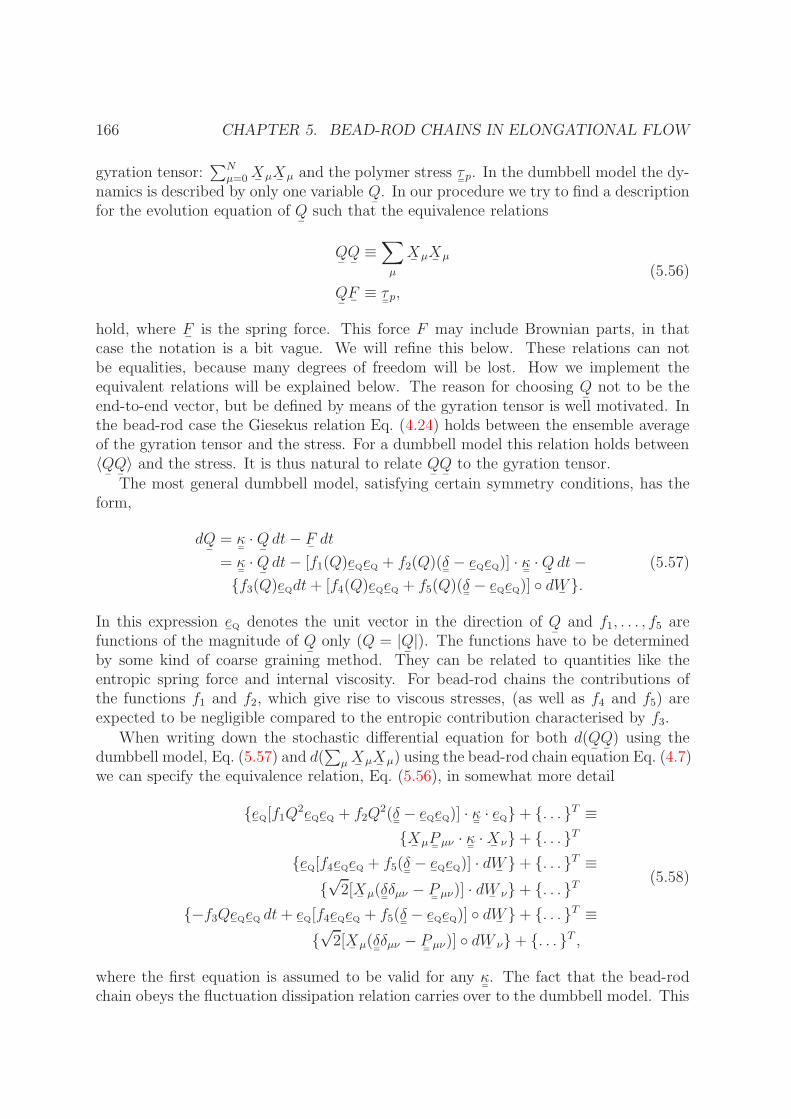
166 CHAPTER 5. BEAD-ROD CHAINS IN ELONGATIONAL FLOW
gyration tensor:∑N
µ=0X¯µX
¯µ and the polymer stress τ
¯p. In the dumbbell model the dy-
namics is described by only one variable Q¯. In our procedure we try to find a description
for the evolution equation of Q¯
such that the equivalence relations
Q¯Q¯≡∑
µ
X¯
µX¯
µ
Q¯F¯≡ τ
¯p,
(5.56)
hold, where F¯
is the spring force. This force F may include Brownian parts, in thatcase the notation is a bit vague. We will refine this below. These relations can notbe equalities, because many degrees of freedom will be lost. How we implement theequivalent relations will be explained below. The reason for choosing Q
¯not to be the
end-to-end vector, but be defined by means of the gyration tensor is well motivated. Inthe bead-rod case the Giesekus relation Eq. (4.24) holds between the ensemble averageof the gyration tensor and the stress. For a dumbbell model this relation holds between〈Q¯Q¯〉 and the stress. It is thus natural to relate Q
¯Q¯
to the gyration tensor.
The most general dumbbell model, satisfying certain symmetry conditions, has theform,
dQ¯
= κ¯·Q¯dt− F
¯dt
= κ¯·Q¯dt− [f1(Q)e
¯Qe¯
Q + f2(Q)(δ¯− e
¯Qe¯
Q)] · κ¯·Q¯dt−
f3(Q)e¯
Qdt+ [f4(Q)e¯
Qe¯
Q + f5(Q)(δ¯− e
¯Qe¯
Q)] dW¯.
(5.57)
In this expression e¯
Q denotes the unit vector in the direction of Q¯
and f1, . . . , f5 arefunctions of the magnitude of Q
¯only (Q = |Q
¯|). The functions have to be determined
by some kind of coarse graining method. They can be related to quantities like theentropic spring force and internal viscosity. For bead-rod chains the contributions ofthe functions f1 and f2, which give rise to viscous stresses, (as well as f4 and f5) areexpected to be negligible compared to the entropic contribution characterised by f3.
When writing down the stochastic differential equation for both d(Q¯Q¯) using the
dumbbell model, Eq. (5.57) and d(∑
µX¯µX
¯µ) using the bead-rod chain equation Eq. (4.7)
we can specify the equivalence relation, Eq. (5.56), in somewhat more detail
e¯
Q[f1Q2e¯
Qe¯
Q + f2Q2(δ
¯− e
¯Qe¯
Q)] · κ¯· e¯
Q+ . . . T ≡X
¯µP¯
µν · κ¯·X
¯ν+ . . . T
e¯
Q[f4e¯
Qe¯
Q + f5(δ¯− e
¯Qe¯
Q)] · dW¯+ . . . T ≡
√
2[X¯
µ(δ¯δµν − P
¯µν)] · dW
¯ν+ . . . T
−f3Qe¯
Qe¯
Q dt+ e¯
Q[f4e¯
Qe¯
Q + f5(δ¯− e
¯Qe¯
Q)] dW¯+ . . . T ≡
√
2[X¯
µ(δ¯δµν − P
¯µν)] dW
¯ν+ . . . T ,
(5.58)
where the first equation is assumed to be valid for any κ¯. The fact that the bead-rod
chain obeys the fluctuation dissipation relation carries over to the dumbbell model. This

5.A. COARSE GRAINING TO A DUMBBELL MODEL 167
can be verified by performing some Ito calculus, which will result in
f 24 = 2(1− f1)
f 25 = 2(1− f2).
(5.59)
The problem is thus reduced to finding three functions only.To convert the equivalence relations into functional relations we use the following
procedure. We set
Q¯Q¯
=∑
µ
X¯
µX¯
µ. (5.60)
Both at the left-hand side and the right-hand side of the relations Eq. (5.58) we performcontractions over the tensor indices to obtain scalar relations. By taking inner prod-ucts with Q
¯Q¯
on the left-hand side and∑
µX¯µX
¯µ on the right-hand side one restricts
the tensor equalities to the direction of Q¯. Making the contraction subsequent to this
projection gives other equalities. Combining the results one finds a full set of equations
f1Q4 = (X
¯µ ·X
¯ν)P
¯µν :
∑ζ
X¯
ζX¯
ζ
f1Q2 + 2f2Q
2 = Tr(P¯
µν)X¯
µ ·X¯
ν
−f3Q+1
2f4(f4 + f ′
4Q+ 2f5) =√
2[X¯
µ(δ¯δµν − P
¯µν)] dW
¯ν −√
2[. . . ] · dW¯
ν
(5.61)
Of course there is not a one-to-one relation between Q and f1, . . . , f3 found in thisway. For different conformations of the bead-rod chain different values are found. Toconstruct the functions, we bin the values found for a specific Q, e.g. for f1 this gives
f1(Q) = 〈 f1(X¯
µ) δ[Q(X¯
µ)−Q] 〉∆f1(Q) =
√〈 f 2
1 (X¯
µ) δ[Q(X¯
µ]−Q) 〉 − f 21 (Q).
(5.62)
Here ∆f1 is the deviation. The relation between f1 andQ is only to a good approximationfunctional when ∆f1(Q) f1(Q).
To obtain the functional relation we performed bead-rod simulations of both station-ary elongational flow and stationary shear, at different rates. We found that, as in thesesimulations no kinked structures are present, the relations turn out to be independentof the flow type and strength. In Fig. 5.24 we plotted the functions f1 and f2. Bothf1 and f2 are small compared to 1. This means internal viscous effects are negligible,which is something we already described in §5.8. Only when the maximum extensionis approached, f1 → 1. Because the elastic force does not diverge (the elastic stress isfinite), at very high deformation rates, this term has to prevent the dumbbell from beingextended beyond its maximum length.
The elastic force f3 is depicted in Fig. 5.25. It is shown that for small values of Q,the deviation ∆f3 is significant compared to the value of f3. This means that in thecoiled state the dumbbell model is not expected to reproduce the results for the Kramers

168 CHAPTER 5. BEAD-ROD CHAINS IN ELONGATIONAL FLOW
f1(Q)f1(Q)
Q=N
f 1(Q)
10.90.80.70.60.50.40.30.20.10
1
0.1
0.01
0.001
0.0001
f2(Q)f2(Q)
Q=N
f 2(Q)
10.90.80.70.60.50.40.30.20.10
0.1
0.01
0.001
0.0001
Figure 5.24: For f1 and f2 the deviations from the expectation values given by ∆f1 and ∆f2 are small.This indicates that a functional relation exists. The internal dissipative effects in a bead-rod chain canbe modelled well by a dumbbell model. The graphs also show that these effects are of minor importance,because the functions are much smaller than 1. Only at near extension f1 approaches one. In nearextension this causes the maximum length not to be exceeded.

5.A. COARSE GRAINING TO A DUMBBELL MODEL 169
f3(Q)f3(Q)
Q=N
f 3(Q)
10.90.80.70.60.50.40.30.20.10
1000
100
10
1
0.1
0.01
1
2 26N2L
1(Q=N)
13
26N2L
1(Q=N)
26N2
Q1(Q=N)2
f3(Q)
Q=N
f 3(Q)
10.80.60.40.20
5
4
3
2
1
0
Figure 5.25: In the coiled state a dumbbell model is not a good approximation. This is indicated bythe fact that the deviation form the mean spring force is much larger than the force itself. In the coiledregime a broad spectrum of relaxation times has to be considered. The second graph shows that theelastic spring force is modelled much better by the Warner spring force than by the inverse Langevinlaw.

170 CHAPTER 5. BEAD-ROD CHAINS IN ELONGATIONAL FLOW
coarse grained modelKramers chain
t=1
xx
=N
1010.1102103104105106107108109
103
100
10
1
0.1
0.01
103
104
Figure 5.26: Relaxation of an initially fully stretched chain of 32 rods. The relaxation of the Kramerschain and the coarse grained dumbbell model superimpose.
chain. The cause for this is the spectrum of relaxation times. This can not be capturedin a dumbbell model which has only one relaxation mode near equilibrium.
In the stretched state f3 has FENE-like behaviour. First the spring force rises linearly,later it seems to diverge. In the second graph of Fig. 5.25 this behaviour is comparedwith the Warner force law and the inverse Langevin force law. The Warner spring forcefits f3 much better than the inverse Langevin force. In the linear regime it gives arelaxation time of 0.0385N2. This is of the right order, but a factor 1.35 larger than thelargest relaxation time of a coiled Kramers chain, Eq. (5.3).
In Fig. 5.26 we have plotted the relaxation of an initially stretched chain, togetherwith that of the dumbbell model. An interpolation function obtained from the numericalexperiment is used for f1, f2 and f3. The two relaxation curves agree well.

Bibliography
[1] O. Hassager. Kinetic theory and rheology of bead-rod models for macromolecularsolutions. I. Equilibrium and steady flow properties. J. Chem. Phys., 60(5):2111–2124, 1974.
[2] O. Hassager. Kinetic theory and rheology of bead-rod models for macromolecularsolutions. II. Linear unsteady flow properties. J. Chem. Phys., 60(10):4001–4008,1974.
[3] M. Fixman and J. Kovac. Dynamics of stiff chains. II. Freely jointed chain. J.Chem. Phys., 61(12):4950–4954, 1974.
[4] D. Acierno, Titomanlio G. and G. Marrucci Dilute solution rheology of flexiblemacromolecules (bead-rod model). J. Polym. Sci. (Polym. Phys. Ed.), 12:2177–2187, 1974.
[5] J.M. Rallison and E.J. Hinch Do we understand the physics in the constitutiveequation. J. Non-Newtonian Fluid Mech., 29:37–55, 1988.
[6] R.G. Larson. The unraveling of a polymer chain in a strong extensional flow.Rheology Acta, 29:371–384, 1990.
[7] E.J. Hinch. Uncoiling a polymer molecule in a strong extensional flow. J. Non-Newtonian Fluid Mech., 54:209–30, 1994.
[8] D.H. King and D.F. James. Analysis of the rouse model in extensional flow. ii.stresses generate in sink flow by flexible macromolecules and by finitely extendedmacromolecules. J. Chem. Phys., 78(4749-4754), 1983.
[9] G. Ryskin. Calculation of the effect of polymer additive in a converging flow. J.Fluid Mech., 178:423–440, 1987.
[10] D.F. James and J.H. Saringer. Extensional flow of dilute polymer solutions. J.Fluid Mech., 97(4):655–671, 1980.
[11] N.V. Orr and T. Sridhar. Probing the dynamics of polymer solutions in extensionalflow using step strain rate experiments. J. Non-Newtonian Fluid Mech., 82:203–232,1999.
171

172 BIBLIOGRAPHY
[12] P. Grassia and E.J. Hinch. Computer simulations of polymer chain relaxation viaBrownian motion. J. Fluid Mech., 308:255–88, 1996.
[13] P.S. Doyle, E.S.G. Shaqfeh and A.P. Gast. Dynamic simulation of freely drainingflexible polymers in steady linear flows. J. Fluid Mech., 334:251–291, 1997.
[14] J.M. Rallison. Dissipative stresses in dilute polymer solutions. J. Non-NewtonianFluid Mech., 68:61–83, 1997.
[15] P.S. Doyle, E.S.G. Shaqfeh , McKinley G.H. and S.H. Spiegelberg Relaxation ofdilute polymer solutions following extensional flow. J. Non-Newtonian Fluid Mech.,76:79–110, 1998.
[16] P.S. Doyle and E.S.G. Shaqfeh Dynamic simulation of freely-draining, flexible bead-rod chains: Start-up of extensional and shear flow. J. Non-Newtonian Fluid Mech.,76:43–78, 1998.
[17] R.G. Larson, Hua Hu, D.E. Smith and S. Shu. Brownian dynamics simulations ofa DNA molecule in an extensional flow field. J. Rheology, 43(2):267–304, 1999.
[18] L. Li, R.G. Larson and T. Shirdar. Brownian dynamics simulations of dilutepolystyrene solutions. J. Rheology, 44(2):291–322, 2000.
[19] R.K. Gupta, D.A. Nguyen and T. Sridhar. Extensional viscosity of dilutepolystyrene solutions: Effects of concentration and molecular weight. Phys. Fluids,12(6),1296–1318, 2000.
[20] D. Frenkel and B. Smit. Understanding Molecular Simulation (From Algorithms toApplications). Academic Press, San Diego, 1996.
[21] G.K. Batchelor. Slender-body theory for particles of arbitrary cross-section in stokesflow. J. Fluid Mech., 44(3):419–440, 1970.
[22] G.K. Batchelor. The stress generated in a non-dilute suspension of elongated par-ticles in pure straining motion. J. Fluid Mech., 46(4):813–829, 1971.
[23] T.T. Perkins, D.E. Smith and S. Chu. Direct observation of tube like motion of asingle polymer chain. Science, 264:819–826, 1994.
[24] T.T. Perkins, R.S. Quake, D.E. Smith and S. Chu. Relaxation of a single DNAmolecule observed by optical microscopy. Science, 264:822–826, 1994.
[25] D.E. Smith, T.T. Perkins, and S. Chu. Self-diffusion of an entangled DNA moleculeby reptation. Phys. Rev. Lett., 75(22):4146–4149, 1995.
[26] T.T. Perkins, D.E. Smith, R.G. Larson and S. Chu. Stretching of a singled tetheredpolymer in a uniform flow. Science, 268:83–87, 1995.

BIBLIOGRAPHY 173
[27] T.T. Perkins, D.E. Smith and S. Chu. Single polymer dynamics in an elongationalflow. Science, 276:2016–2021, 1997.
[28] S.R. Quake, H. Babcock and S. Chu. The dynamics of partially extended singlemolecules of DNA. Nature, 338:151–154, 1997.
[29] D.E. Smith and S. Chu. Response of flexible polymers to a sudden elongationalflow. Science, 281:1335–1350, 1998.
[30] D.E. Smith, H.P. Babcock and S. Chu. Single polymer dynamics in steady shearflow. Science, 283:1724–1727, 1999.
[31] R.G. Larson, T.T. Perkins, D.E. Smith and S. Chu. Hydrodynamics of a DNAmolecule in a flow field. Phys. Rev. E, 55(2):1794–1797, 1997.
[32] T. Sridhar, V. Tirtaatmadja, D.A. Nguyen and R.K. Gupta. Measurement of exten-sional viscosity of polymer solutions. J. Non-Newtonian Fluid Mech., 40:271–280,1991.
[33] J. van Nieuwkoop and M.M.O. Muller von Czernicki. Elongation and subsequentrelaxation measurements on dilute polyisobutylene. J. Non-Newtonian Fluid Mech.,67:105–123, 1996.
[34] S.H. Spielberg and G.H. McKinley. Stress relaxation and elastic decohesion ofviscoelastic polymer solutions in extensional flow. J. Non-Newtonian Fluid Mech.,67:49–76, 1996.
[35] N.V. Orr and T. Sridhar. Stress relaxation in uniaxial extension. J. Non-NewtonianFluid Mech., 67:77–103, 1996.
[36] V. Tirtaatmadja and T. Sridhar. Comparison of constitutive equations for polymersolutions in unaxial extension. J. Rheology, 39(6):1133–1160, 1995.
[37] M.R.J. Verhoef, B.H.A.A. van den Brule and M.A. Hulsen. On the modelling ofPIB/PB boger fluid in extensional flow. J. Non-Newtonian Fluid Mech., 80(2-3):155–182, 1999.
[38] I. Ghosh, R.C. Armstrong, R.A. Brown and G.H. McKinley. Modelling dilute poly-mer solutions in extensional flows at intermediate strains. presentation, 1999.

174 BIBLIOGRAPHY

Chapter 6
Reptation
6.1 Introduction
Reptation theory describes the rheological behaviour of linear polymers in highly mu-tually entangled conformations. Entanglements are created only when the density ofpolymers is high enough. This means that the polymeric liquid we will be consider-ing here is a melt or a highly concentrated solution. A second important condition forentanglements to arise is a large molecular weight.
The notion of entanglements first arose in the molecular theory of rubber elasticity.The linear response to deformations of an elastic solid is characterised by the elasticmodulus G0, τxy = G0γ. This modulus is proportional to kT times the number ofdegrees of freedom per unit volume that do not relax subsequent to the deformation.Early molecular-based theories of rubber elasticity describe the rubber as composedof ghost-chains. A strand between crosslinks is modelled to have the same amount ofconfiguration space available, as if no neighbouring chains are present. Because ghost-chains are not restricted when sampling phase space, the number of non-relaxed degreesof freedom equals the number of crosslinks per unit volume. The relaxation modulus isthus proportional to the number of crosslinks.
For systems where the polymer strands between crosslinks are long, the elastic mod-ulus calculated in this way is much smaller than experimentally observed values. Thereason for this is the entanglement of chains with neighbouring chains. This entangledstate makes it impossible for a strand (between crosslinks) to sample as large a piece ofphase space as a polymer without neighbours. The entanglements give rise to topolog-ical constraints. The neighbours do not only hinder the movement of the strand, theyactually make it impossible for the chain to sample as large a space as a ghost-chain.This results in a reduction of the entropy and consequently the elastic modulus is in-fluenced. For a highly entangled state the number of degrees of freedom that can notrelax to equilibrium, after a deformation is applied, is proportional to the number ofentanglements. Thus
G0 = kTc
Ne, (6.1)
175

176 CHAPTER 6. REPTATION
Figure 6.1: The black polymer is constrained in its sidewise motion because of entanglements withneighbouring chains. A tube is used to model the space the polymer can sample without crossing the(semi) topological constraints. The picture is somewhat misleading because the tube cross-section willbe much wider than the one depicted here.
where c is the number of monomers per unit volume and Ne can be interpreted as thenumber of monomers in a strand between two entanglement points (in fact Eq. (6.1) isthe experimental definition of Ne).
In this setting of rubber elasticity Edwards [1] first introduced the tube-picture. Astrand between crosslinks is modelled as if it is surrounded by a tube. The tube denotesthe fraction of configuration space the strand can sample. It is characterised by one typ-ical length scale a, often called the tube-diameter (for the reason for this see appendix6.B). It is the typical distance between entanglements. The length scale not only charac-terises the diameter of the tube but also a step size. Because entanglements are thoughtto be distributed randomly the tube is taken to have a random walk configuration withstep size a.
The idea of the tube was carried over to the field of polymer melts by De Gennes[2]. Now polymers are not connected by crosslinks anymore (at least not permanently).Entanglements no longer constitute permanent constraints. Therefore the tube is nolonger permanent. Sidewise motion is constrained but motion along the contour of thetube is not constrained. Subsequent to a deformation the stretch of polymer chains willrelax quickly. Changes in orientation are much slower. The relaxation of orientation canonly proceed via diffusion of the chain out of the tube. This motion was termed reptationby De Gennes. When the chain reptates out at one side a new tube segment is createdat this location (illustrated by Fig. 6.3). At the other side a part of the tube disappears.Based on this picture Doi and Edwards developed their constitutive equation [3, 4, 5](discussed in §6.2).
When increasing molecular weight (i.e. increasing chain length) a polymer melt willmake the transition from an unentangled state to an entangled state. After this tran-
6.1. INTRODUCTION 177
sition there will be a split in time scales. The time scale corresponding to stretchrelaxation will be comparable to the relaxation of an unentangled polymer. The timescale corresponding to relaxation of orientation, the reptation or disengagement time τd,is much larger. According to the (pure) reptation picture it scales as M3. For time scalessomewhere between the stretch time and the reptation time not much happens. In thisrange of time scales the response is characterised by a constant value of the relaxationmodulus, the rubber plateau modulus, which scales as Eq. (6.1). This modulus does notdepend on the molecular weight (G0 ∝ M0) only on entanglement density.
One of the most famous graphs supporting reptation theory is Fig. 6.2. It clearlyillustrates the transition in the dynamics when increasing the molecular weight. Inthe unentangled state the viscosity is proportional to M and in the entangled regimeit is proportional to M3.4. Reptation predicts M3 (∝ G0τd), which is as close to theexperimental value as one might expect of such a simple theory. On the other hand thedeviation indicates that there is more to melt rheology than reptation only. Doi firstidentified the 0.4 deviation in the exponent as a possible end-effect [7]. Fluctuations ofthe chain length near the ends of the tube cause extra rapid relaxation of the orientationthere. Doi’s treatment of tube length fluctuations gave however a too narrow range ofmolecular weights where the 3.4 exponent is valid. In the description of Milner andMcLeish [8] this shortcoming is no longer present.
The Doi-Edwards equation makes a number of predictions that are at least quali-tatively correct. These results have convinced the majority of researchers in the fieldthat the tube-picture is the most promising road toward a quantitative description ofrheology of entangled polymer systems. However, the Doi-Edwards model also makespredictions that are completely off. One important example is the excessive shear thin-ning that is predicted. The model predicts that for high shear rates the stress decreaseswith increasing shear rates. This is in fact not found in experiments. Although theviscosity of melts is very shear thinning the stress itself always increases with increasingshear rates. These, and other mispredictions, are now thought to be caused by the lackof self-consistency of the Doi-Edwards model. The surrounding chains also relax causinga certain amount of relaxation of the tube constraint.
Doi and Edwards assumed that the lack of self-consistency only gives minor errors.This turned out not to be true. In branched polymers the effect even gives rise to thedominant relaxation mechanism: dynamic dilution. For polydisperse systems relaxationof neighbouring polymers gives rise to the double reptation mechanism [9, 10]. Butalso for monodisperse linear polymers the relaxation of neighbouring polymers is im-portant, especially at high shear rates. The dominant mechanism by which constraintsare released at high shear rates was named convective constraint release by Marrucci[11]. It counteracts the strong alignment which gives rise to the excessive shear thinningpredicted by the Doi-Edwards equation.
The last few years there has been significant progress in the development of con-stitutive relations for entangled polymeric systems. The first major step forward is theidentification of (probably) all important relaxation mechanisms. The last of these is theconvective constraint mechanism proposed by Marrucci. The second step forward is the

178 CHAPTER 6. REPTATION
-1 0 1 2 3 4 5
cons
tant
+ lo
g η 0
constant + log M
polystyrene
polyvinyl acetate
polyethylene glycol
polymethylmethacrylate
polytetra-methylp-silphenylenesiloxane
polybutadiene
polyethylene
polyiso-buthylene
polydi-methylsiloxane
M 1.0
M 3.4
Figure 6.2: A famous picture in reptation theory (from [6]). For a large range of different linear polymermelts the dependence of viscosity on molecular weight shows similar scaling. For small M the viscosityincreases linearly with M . For large M the viscosity scales as M3.4. This change in dynamics is causedby the occurrence of entanglements when M becomes large enough. Reptation theory tries to describethe dynamics of highly entangled polymer melts.

6.2. THE DOI-EDWARDS MODEL 179
increasing quantitative accuracy of the predictions. This is especially the case for linearrheological behaviour. Milner and McLeish have made impressively accurate predictionsfor the linear rheology of star-polymer systems [12, 13], and also for linear polymers [8].A third development has to do with the applicability of constitutive equations. Onlyrecently the equations can be incorporated into macroscopic flow simulations. The con-figuration fields method [14] has made it possible to incorporate kinetic theory basedmodels into macroscopic simulations.
For most models of entangled systems the deformation fields method, which will betreated in chapter 7, is more appropriate. The deformation fields method is a method toincorporate so called integral constitutive equations into flow calculations. These modelsconstruct the stress in a fluid element by performing an integral over its deformationhistory. The Doi-Edwards equation is such a model.
In this chapter we will start with discussing the ingredients needed to describe aentangled polymeric system. The final goal is to develop a constitutive equation thatincorporates all important effects and that can also be implemented into a deformationfields code. This last point is essential for numerical simulations of complex flow fields.
We believe that segment connectivity is a very important property that has to bemodelled correctly. It is well known that in the double step strain experiment theDoi-Edwards equation is not valid. This is caused by the lack of connectivity in thismodel (i.e. the independent alignment approximation). In real flows the deformationhistory of a fluid element is so complicated that effects such as double step strain will beimportant. Furthermore important relaxation effects that occur at endpoints, such asthe so-called contour length fluctuations, are currently only modelled well in the linearrheological regime, see [8]. In our description these effects are also modelled accuratelyin the nonlinear regime.
The demand of incorporating chain connectivity forces a special form upon the for-malism. Especially the description of the reptative motion is cast in a somewhat unfamil-iar form (but is still highly accurate). Although we will gradually develop a constitutiveequation when the chapter progresses, we do not consider this as the final equation. Wenote that, even in the current state of development of reptation theory, there are stillfundamental problems with the description of the so-called constraint release mecha-nism in the nonlinear regime. We will discuss these problems in appendix 6.A. Not theequation itself is important, but the methodology. The developed methodology can beused for a larger class of systems, not only monodisperse linear polymers but also e.g.polydisperse branched polymers.
6.2 The Doi-Edwards model
The Doi-Edwards constitutive equation is based on the tube-picture, making the mostsimple assumptions.
In this section we will give a detailed derivation of the Doi-Edwards. The reason wedo this is because our formalism is aimed at repairing a flaw that is present in the Doi-Edwards equation (which has to do with chain retraction). Besides repairing the flaw,

180 CHAPTER 6. REPTATION
we will add some relaxation mechanisms which are believed to be important but are notincluded in the Doi-Edwards equation. During the derivation it will become clear whatapproximations are made and which effects are not included. In §6.3 the basic formalismwill be presented. In the next section §6.4 it is shown how this formalism can be usedto repair the flaw present in the Doi-Edwards equation.
If one makes a snapshot of a polymer in an entangled melt in equilibrium one seesno evidence for a characteristic length scale a (the tube diameter). Because a chain issurrounded by chains with identical chemical properties (i.e. in a melt), the equilibriumstatistics are the same as for a chain submerged in a theta solvent. This means that,when considering long enough length scales, a chain can be modelled as a random walk,characterised by a Kuhn step b. The root mean square of the end-to-end distance is
〈R2〉 = b2N, (6.2)
where N is the number of Kuhn steps.In most practically relevant situations the Kuhn step b is much smaller than a. This
means that a tube segment of length a contains many Kuhn steps. Strands of chainsinside a tube segment will therefore never be far from equilibrium. For this reason thechain strands can be described as linear entropic springs. Because of the dense packing ofpolymer chains the movement of a segment does not create a flow field. Hydrodynamicinteraction is screened. The dynamics inside the tube is therefore characterised by asimple Rouse spectrum (and not a Zimm spectrum).
The Rouse time τR, i.e. the largest time of the Rouse spectrum, corresponds roughlyto the equilibration time of polymers with similar molecular weights but in an unentan-gled state. In an entangled state nothing much happens for times in between the Rousetime and a reptation time τd. The chain inside the tube is relaxed, but a correlation oftypical length a in the conformation persists. In this range the tube becomes observable.The extra tension created by the prevention of the relaxation of this degree of freedomis
F =3kT
a(6.3)
(this formula can be taken as the definition of a). The magnitude of the tension is easilyunderstood. It takes O(kT ) of energy, ≈ F ·a, to keep a degree of freedom from relaxing.
The tension has a thermodynamic/entropic origin. It decreases the number densityof monomers within a tube segment. Therefore the entropy per monomer increases,counteracting the decrease in entropy caused by the tube constraint. The total entropyinside the tube will become equal to the entropy of a monomer outside the tube (i.e. atthe chain ends). The exact calculation of the ‘chain-in-a-tube’-statistics is performed in[15].
The length scale a can be used to define a new random walk with step size a. Thisrandom walk is called the primitive chain (or also primitive path). Its contour lengthL (measured with a ruler of length a) can be obtained by considering the end-to-enddistance
b2N = a2(L/a) = aL (6.4)

6.2. THE DOI-EDWARDS MODEL 181
Figure 6.3: The (pure) reptation picture of a step strain. When applying a rapid deformation boththe primitive chain and the surrounding tube deform affinely. In a Rouse time he chain retracts to itsequilibrium length. On longer time scales the chain escapes the confining tube by means of reptativemotion. Now the residual stress relaxes.
The number of tube segment of length a per chain is L/a = (b2/a2)N . For realistic meltsthis number ranges somewhere between 20 and 200. The number of Kuhn steps withinone tube segment is a2/b2. The equilibrium ‘Kuhn-step-density’ per unit tube length isthus
n = a/b2. (6.5)
The main thought experiment in developing the Doi-Edwards equation is that ofthe single step strain deformation and subsequent relaxation. The experiment has threestages. First the deformation, then stretch relaxation on a Rouse time scale followed byorientational relaxation by reptation (see Fig. 6.3).
For the deformation step one assumes that the step is performed so quickly thatno relaxation occurs on this time scale. The deformation is therefore affine (for longenough length scales such as a). Furthermore it is assumed that the deformation is notthat large that finite extensibility effects of the chain become important (i.e. the Henckystrain ε log(N)). In this limit the Rouse description stays valid for the chain insidethe tube.
Not only the chain one is considering, but also the surrounding chains (constitutingthe tube) deform affinely. This results in the observation that the tube deforms affinelyas well. The way this is described is by posing that individual tube segments deformaffinely. This last statement contains a rather strong assumption, which is not madeexplicitly in the Doi-Edwards paper [3].
In the Doi-Edwards papers a switching between two mental pictures is used. Thefirst picture is that of the tube. The other is that of slip links. In the second pictureentanglements are modelled as slip links through which the chain can move without

182 CHAPTER 6. REPTATION
friction. During the deformation step the slip links are displaced affinely. These slip linksnow constitute the new endpoints of the chain segments. The important question that isnot raised in the papers is whether the entanglements before and after the deformationare caused by the same neighbouring chains. (If this is the case the slip link picture isnot a good analogue).
After affine deformation of both the tube and the chain inside this tube, the chain isno longer in thermodynamic equilibrium. Doi and Edwards assume that the equilibriumtension in the deformed tube equals the equilibrium tension. Their hand waving argu-ment for this is that, for a stretched tube segment, the number of entanglements perunit length is decreased, but that in the perpendicular direction neighbouring polymersare squeezed inward. According to them it is reasonable to assume the net effect iszero. The entropically generated tension in the deformed state equals the equilibriumtension, Eq. (6.3). The chain retracts until the entropic spring forces balance the tensionEq. (6.3). This process occurs in the order of a Rouse time. The net effect is that thenumber density of monomers in a tube segment relaxes back to the equilibrium value.
Within the Doi-Edwards picture a deformation step followed by retraction can beput into mathematical terms with relative ease. Let us start with an equilibrium chainsegment characterised by its end-to-end vector Q
¯0, which connects two ‘entanglement-
points’. This vector is a random, isotropically (presumably Gaussian) distributed vectorwith an average length a. After affine deformation this segment becomes
Q¯
= F¯·Q¯
0, (6.6)
where F¯
is the deformation-gradient tensor.After the relaxation of the stretch, which occurs in a few Rouse times, the chain in
the segments have equilibrium tension (and equilibrium monomer density). The stresscontribution of a single segment is readily identified as (tension time direction times theconnector vector)
F¯Q¯
=3kT
a
Q¯Q¯|Q
¯| . (6.7)
The number of Kuhn steps in one segment is (a/b2)|Q¯|, using Eq. (6.5). Let c be the
density of Kuhn steps per unit volume in the melt. (This is of course directly proportionalto the number of monomers per unit volume). Then the mean number of segments perunit volume becomes
cb2
a
1
〈|Q¯|〉 . (6.8)
The stress tensor is given by (something like n〈F¯Q¯〉):
τ¯
p = 3b2
a2c kT
⟨Q¯Q¯|Q
¯|⟩/〈|Q
¯|〉 = 3
b2
a2c kTQ
¯. (6.9)
Here the tensor Q¯
is the so called Q¯-tensor. This tensor denotes the mean orientation.
The average denotes an average over all possible initial values Q¯
0, which are isotropically

6.2. THE DOI-EDWARDS MODEL 183
distributed. Because the length of Q¯
0 drops out of the expression one can use a vectoruniformly distributed on a random sphere. Linearising the stress expression for smallshear strains γ, gives τxy = 4/5(b2/a2) c kTγ, thus
G0 =4
5
b2
a2c kT. (6.10)
Comparing this expression with Eq. (6.1) gives Ne = 5a2/4b2, with Ne the number ofKuhn steps instead of monomers.
Immediately after the fast relaxation of the stretch all surviving segments contributeto the stress. Thereafter newly created segments do not contribute to the stress, becausethese do not have a preferred direction. To be able to calculate the stress one has toknow how many of the original tube segments are still present at a later time.
At every moment in time the position of tube segment along the total tube contour(with length L) can be characterised by a variable s. The left tube-end is denoted bys = 0, the middle by s = 1. For time steps larger than the Rouse time, the length of theprimitive chain can be taken to be constant. The only relevant motion is centre-of-massdiffusion in the tube. For a specific tube segment the change of s is therefore describedby the stochastic differential equation
dS =
√2Dc
L/2dW, (6.11)
where Dc is the curvilinear centre-of-mass diffusion tensor. We here use the standardconvention to indicate stochastic processes with an uppercase, here S. (Note that thedimensionful position is LS/2.) According to the fluctuation-dissipation theorem, ormore precisely the Einstein relation, the diffusion tensor is proportional to kT dividedby a friction coefficient. This friction coefficient has a linear dependence on the numberof monomers in the chain, thus Dc ∝ 1/L ∝ M−1. For all segments of one tube thisequation Eq.(6.11) holds with the same Wiener process, only the initial value of S differs.If S = 0 (or S = 2 which is the other segment end) the segment is annihilated and a newone is created. The probability that at a position s a segment is present that alreadyexisted at t = 0 obeys the diffusion equation
∂
∂tp(s, t) =
4Dc
L2
∂2
∂s2p(s, t). (6.12)
with the initial condition p(s, 0) = 1 and the boundary condition for the tube end isp(0, t) = 0. The problem is clearly symmetric around s = 1. Therefore the problemonly has to be considered on s ∈ [0, 1], with boundary condition ∂
∂sp(1, t) = 0. This
diffusion problem can easily be solved by a Fourier decomposition using base functionsof the form
√2 sin[(π/2 + pπ)s],
p(s, t) =
∞∑p=0
4
π(1 + 2p)sin[(π/2 + pπ)s] exp
[−π
2Dc
L2(1 + 2p)2t
]. (6.13)

184 CHAPTER 6. REPTATION
10 1
10 2
10 3
10 0 10 1 10 2 10 3
h-1(γ
) G
(t,γ
) [P
a]
t [sec]
τR
GDE(t)
τd
10 1
10 2
10 3
10 0 10 1 10 2 10 3
h-1(γ
) G
(t,γ
) [P
a]
t [sec]
τR
GDE(t)
τd10 -2
10 -1
10 0
10 -1 10 0 10 1
h(γ)
γ
Figure 6.4: Left: relaxation after a shear step, for different strains γ. The shear stress is plotted asfunction of time (experimental data from [16]). The stress is scaled by an amount h(γ)γ. For timeslarger than τR a perfect superposition is observed. The damping function h(γ) is plotted in the rightgraph (the points are the experiments). The function compares favourable with the Doi-Edwards result(solid line), obtained from Eq. (6.9). The so-called independent alignment(dashed line) compares evenbetter.
The probability that a segment present at t = 0 is still present at t is given by
P (t) =
∫ 1
0
p(s, t)ds =∞∑
p=0
8
π2(1 + 2p)2exp
[−π
2Dc
L2(1 + 2p)2t
](6.14)
The largest relaxation time is given by
τd =L2
π2Dc
. (6.15)
Taking the scaling of the curvilinear diffusion coefficient with the number of monomersinto account, one finds that τd ∝ L3 ∝M3.
After a step strain and the subsequent stretch relaxation, up to t = O(τR), the stressrelaxes further via
τ¯
p(t) =15
4G0Q
¯P (t). (6.16)
This is the stress contributions of the segments times the probability a segment is stillpresent after a time t. This equation shows a time-strain separability of the responsesubsequent to a step strain.
Fig. 6.4 shows experimental results [16] for stress relaxation after a step strain. Thispicture (and especially the right one) is one of the major reasons for the popularity ofthe tube-picture. The left graph illustrates time strain separability. For times t > τRafter a step shear strain γ is applied, the shear stress can be written as
τxy(t) = G(t)h(γ)γ. (6.17)

6.2. THE DOI-EDWARDS MODEL 185
The right graph shows the so-called damping function h(γ). The damping function is afingerprint of the Q
¯-tensor, h(γ) = 15/4Qxy/γ. It agrees very well with the dependence
predicted by the Doi-Edwards Q¯-tensor. The fast decrease for large strains demonstrates
the extreme alignment of tube segments for large deformations. The theoretical predictedrelaxation modulus,G(t) = G0P (t), is however not at all in accordance with experiments.The reason is that in the Doi-Edwards model the mode corresponding to the largestrelaxation time contains almost all the stress (81% = 8/π2). This means importantfaster relaxation mechanisms are missed in the pure reptation picture.
The equation for a step strain can be easily generalised to a constitutive equation(there is however a flaw in this derivation that will be discussed below). The first stepis to think about the meaning of P (t − t′), where t′ is a reference time. This is theprobability that a segment that was created before time t′ survived until the presenttime t. The survival probability of segments created in the interval [t′, t′ + ∆t′] equalsP (t−(t′+∆t′))−P (t−t′). This is the probability that segments were present at (t′+∆t′)are still present at t minus the contribution of segments that were already present beforetime t′. This thus selects the segments created in [t′, t′ + ∆t′]. The survival probabilitydensity of segments created at t′ thus becomes
µ(t− t′) =d
dt′P (t− t′) = − d
dtP (t− t′). (6.18)
At the moment of creation a segment obeys isotropic statistics. At a later time t thesegment is affinely deformed via the deformation gradient-tensor with respect to t′:F¯(t, t′) · Q
¯t′ (where Q
¯t′ comes from the isotropic equilibrium distribution). The contri-
bution of segments created at t′ to the stress is
15
4G0 µ(t− t′)Q
¯(t, t′). (6.19)
The Q¯
tensor is calculated by applying Eq. (6.9), inserting Eq. (6.6) for F¯(t, t′) and
average isotropically over Q¯
t′ (i.e. Q¯
0 in Eq. (6.6)). The total stress thus becomes
τ¯
p(t) =15
4G0
∫ t
−∞µ(t− t′)Q
¯(t, t′)dt′. (6.20)
This equation is often called the Doi-Edwards constitutive equation. It belongs to theclass of time-separable Rivlin-Sawyers equations (or even more narrow the class of time-separable K-BKZ-equations). The validity is restricted to situations where Rouse timedynamics can be discarded. This means that the shear rate has to be significantly smallerthan 1/τR. If one wants to consider more rapid flows internal Rouse dynamics has to beaccounted for. In the simplest case this gives one extra equation for a stretch parameter,see §6.6.
Even within the setting of the idealised reptation picture equation Eq. (6.20) hasa serious flaw. There are two mechanisms by which tube segments can be destroyed.The first is reptation. This is modelled correctly. The second one is instantaneousequilibration of the primitive chain contour length. This process is incorporated into

186 CHAPTER 6. REPTATION
Observation Ingredients needed in model SectionTime-strain separability Doi-EdwardsStep-shear (damping function) Doi-EdwardsLinear viscoelasticity contour length fluctuation §6.3
+dynamic dilutionOvershoots τxy, N1 after step-shear stretch §6.6Steady shear convective constraint release §6.A.2Stress relaxation convective constraint release §6.A.2after cessation steady shearΨ = −N2/N1 behaviour the strain measure (Q
¯-tensor) §6.B
Undershoot extinction angle segment connectivity §6.4after step down shear rateDouble step-strain segment connectivity §6.4
Table 6.1: To incorporate experimental observations done in melts into a reptation-constitutive equationalterations to the Doi-Edwards equation are required. This summation is inspired on similar ones inthe papers [17, 18, 19, 8].
the Q¯-tensor. However, when the chain retracts, the segments near the tube ends are
destroyed first. Saying that all segments have equal probability of being abandonedwhen the chain retracts is obviously wrong in general.
This is not an issue for the step strain case. All segments there have the samedeformation history. They are isotropically distributed at t = 0, and are all deformedvia F
¯. The portion of segments that do survive after retraction is 〈|Q0|〉/〈|Q|〉. Because
they all hold the same stress it does not matter where they are located along the contour.
In the general case the deformation history differs for segments located at differentpoints along the contour. Therefore the reasoning used in the step strain case is nolonger valid. Segments near the middle are older and thus have experienced more of thedeformation history. The segments near the ends that have a higher probability of beingdestroyed are generally younger and thus have experienced a deformation history thatis shorter. The equation we will propose in this chapter (in §6.4) is aimed at a bettertreatment of this phenomenon.
As discussed in the introduction, many phenomena are not described well in thepure-reptation picture. The most important of these effects are summarised in Tab.6.1,together with the section were they will be treated. Broadly speaking one can identifytwo effects that are missing from the Doi-Edwards equation. The first is end-effects.The chain is more relaxed near the ends. Because in melts the number of entanglementsper tube can easily be as low as 20, these effects are important. The second importantshortcoming in the tube picture is the lack of self consistency. At the same time thatthe chain in a tube relaxes the surrounding chains constituting the tube also relax. Thisgives rise to dynamic dilution and in strong flow to convective constraint release. Wewill now proceed to introduce a formalism which enables us to incorporate these effects.

6.3. RELAXATION MECHANISMS 187
Figure 6.5: There is obvious a one-to-one relation between creation time t′ and position, in a mean sense.Segments are created at the tube-end s = 0. Therefore old segments are expected to be positioned nearthe middle of the tube, and new segments near the ends. When this ordering is imposed rigorously, thefraction of segments that is younger than t equals s(t, t′).
6.3 Relaxation mechanisms
In this section we will introduce the basic approach for the development of the extendedreptation model presented in this chapter. The goal is to incorporate all known relevanteffects in one framework, including chain connectivity. The final equation will still beuseful for doing flow simulations.
In the Doi-Edwards equation Eq. (6.20) tube segments are labelled by their time ofcreation t′. When one wants to create a more advanced picture of reptation it is necessaryto know not only how old a segment is, but also where it is located along the contour.This second labelling is especially essential if one wants to take segment connectivityeffects into account (as is done in §6.4). In the so-called rigorous Doi-Edwards equationthe central quantity is a probability density K(s, t, t′) that gives the probability densityfor a segment at position s to have been created at time t′. The parameter space of Kis too large for it to be useful in a flow calculation. We therefore introduce a relationbetween the position along the contour s and the time of creation t′. The motivation forsupposing that this might give good results is the observation that new tube segmentsare always created at the tube-ends. This means that, when moving inward away froma tube-end, the age of segments increases. In an average sense the oldest segment willbe found in the middle of the tube.
Although it is only valid in an average sense we will pose that the ordering betweencreation time, t′, and the position along the contour, s, is obeyed rigorously. This is themain approximation in our formalism. The survival probability µ(t, t′)dt′ denotes thefraction of all segments present at time t, that is created in the time interval [t′, t′ + dt′].This fraction can be denoted as a fraction ds of the mean tube, where s is the contourvariable∗. As before, s = 0 denotes the tube-end and s = 1 the middle of the tube.
∗This statement is not fully justified as will be discussed in §6.4
188 CHAPTER 6. REPTATION
Using the ordering between creation time and position one finds,
s(t, t′) =
∫ t
t′µ(t, t′′)dt′′ = 1−
∫ t′
−∞µ(t, t′′)dt′′, (6.21)
where s(t, t′) is the position along the contour of a segment with creation time t′. Thisordering is illustrated in Fig. 6.5.
The ordering is fully rigorous if the chain is fixed in the middle. This is for exam-ple the case for the arms of star-polymers. Inner parts can only relax by deep chainbreathing. The end of the embedded chain has first to pass all outer segments before aninner segment can be relaxed. An other example where the ordering is fully correct is ahalf-infinite tube.
For an ordinary tube of finite length, the ordering is expected to be very well obeyednear the tube ends. Near the middle a segment can be originally created at either oneof the two ends of the chain. The oldest segment will not be positioned exactly atthe middle. By demanding the strict relation between t′ and s the segments near themiddle are re-arranged. We will however demand that in absence of other relaxationmechanisms The relaxation is fully equivalent to the Doi-Edwards relaxation. Othereffects, such as chain-length fluctuations, act near the tube-ends. Here the ordering isfully justified. Therefore we expect that the final total relaxation will be described veryaccurately. Effects such as chain length fluctuations that are very difficult to incorporatein other formalisms (even in contour variable descriptions) are easy to include in ourformalism.
The formalism we adopt to describe relaxation mechanisms is that of lifetime distri-butions. For every segment, every relaxation mechanism is characterised by a lifetime,τ(s). The probability that a piece of tube located at a position s is annihilated duringa time step dt equals 1− dt/τ(s). The inverse of the lifetime is an annihilation rate. Ifprocesses are mutually independent the rates add up to one total rate of annihilation
1
τ(s)=
1
τ1(s)+
1
τ2(s)+ . . . . (6.22)
This gives the formalism a certain flexibility. When a relaxation mechanism is missed itcan be added later with relative ease. Also, for architectures different from linear chains,other mechanisms will be dominant. The change in survival probability density of asegment created at time t′, µ(t, t′), is the probability the segment is not yet annihilated,i.e. µ(t, t′), times the rate of annihilation:
d
dtµ(t, t′) = − 1
τ(s)µ(t, t′). (6.23)
Although the relation between t′ and s is not strictly valid for the finite tube, thelifetime distribution τrept(s) will be constructed such that it gives rise to an evolutionequation that gives a µ(t, t′) that is equal to that of the Doi-Edwards equation. Toconstruct τrept(s) we use Eq. (6.23) in a reverse way. Because in the Doi-Edwards case

6.3. RELAXATION MECHANISMS 189
0
0.2
0.4
0.6
0.8
1
0 0.2 0.4 0.6 0.8 1
τ rep
t(s)
/τd
s
π3/8 s2
Figure 6.6: Positional dependence of the life time in the pure (Doi-Edwards) reptation picture. Nearthe tube-ends the time is proportional to the time needed to reach a end by means of diffusive motion.More to the middle the life time of segments becomes invariant of position and equals τd.

190 CHAPTER 6. REPTATION
µ(t, t′) is known, namely by substituting Eq. (6.14) into Eq. (6.18), τrept(s) has to obey
1
τrept(s(t, t′))= − 1
µ(DE)(t− t′)d
dtµ(DE)(t− t′). (6.24)
Here the right-hand side is a function of (t − t′). Using Eq. (6.18) and Eq. (6.21), alsos(t, t′) can be expressed as a function of (t− t′) (for this special case)
s(t, t′) = 1− P (DE)(t− t′), (6.25)
where P (t − t′) is given by Eq. (6.14). Therefore combining Eq. (6.25) and Eq. (6.24)gives an (implicit) relation between between s and τrept(s). This relation is plotted inFig. 6.6.
For small s Eq. (6.14) can be evaluated analytically. This gives P (t) ≈ 1−4π− 32
√t/τd.
In this limiting case
τrept(s) =π3
8s2τd, for s 1. (6.26)
The scaling of τrept(s) with s2 is expected for a problem governed by diffusion. Thecharacteristic time relaxation at position s is proportional to the time needed for achain end to diffuse this distance (by means of curvilinear centre-of-mass diffusion), i.e.τrept ∝ DcL
2s2. For a semi-infinite tube this scaling will persist for any s. In Fig. 6.6 itis shown that the parabolic relation flattens off to τrept(s) = τd for s near 1. In this innerpart of the tube both ends come into reach. The relaxation time becomes invariant ofthe position. This is expected because here the ordering is not fully valid anymore, andtherefore the position is neither well defined.
The chain inside the tube is modelled as a Rouse chain. The length of this chainfluctuates. This fluctuation is believed to give rise to a rapid relaxation of the chain-ends. For a Rouse chain, which is in equilibrium within the tube, the position of theend-bead along the contour varies with time as
〈[S(t)− S(0)]2〉 = 16π− 32
√τRt
τd, for t τR (6.27)
[20, page 212] where the Rouse time is given by
τR =aL
3π2Dc
=a
3Lτd. (6.28)
As time progresses the bead feels more and more of the rest of the chain and the dynamicsslows down with respect to the diffusive motion of a free bead. The position of the end-bead scales with t
14 and not t
12 . At times of O(τR) centre-of-mass diffusion of the whole
chain becomes the dominant motion and the dynamics of pure reptation is recovered.In reptation theory the part of an initial tube that is relaxed, is the part that the
end-bead has passed. When the chain-end passes a constraint it can explore a new tubesegment. The portion of constrained tube can be found by solving a first-pass problem.

6.3. RELAXATION MECHANISMS 191
10 -1
10 0
10 1
10 -5 10 -4 10 -3 10 -2 10 -1 10 0 10 1 10 2 10 3
s(t,0
) L
/ (2
(Dc
τ R)1/
2 )
(t/τR)
2 (N/π)1/2 (t/ τR)1/2
3.65 (t/ τR)1/4
2 π-1/2 (t/ τR)1/2
Figure 6.7: The expectation value of the part of a tube present at t = 0 that is relaxed at later times.This graph is the result of solving the numerical simulation of the first-pass problem for the end-beadof a Rouse chain of 100 and of 1000 segments in a (semi-infinite) tube. The left part of the graph showthe evolution on time scales where the end-bead does not yet feel it is part of a chain. This is not arelevant regime, because this time scale is believed to be very small in real systems O(aL
b2 τR). The t14
regime is a fingerprint of the Rouse dynamics. When time progresses the influence of an increasingpart of the chain is felt by the end-bead. At the order of Rouse times the finite length of the chainbecomes apparent and the centre-of-mass motion dominates the dynamics. The filled black dots denotethe situation where one end of the chain is fixed. The passing of the free end now becomes a highlyactivated process for times that are much larger than τR.

192 CHAPTER 6. REPTATION
The part of the tube that was present at time t = 0 and not present any longer at timet is given by
s(t, 0) = 〈max(S(t′)− S(0)tt′=0)〉. (6.29)
We simulated the first-pass problem for a Rouse chain considering one tube-end only.The results are plotted in Fig. 6.7. The simulation gives for t τR that
s(t, 0) =7.3
π
[τR t
τ 2d
] 14
. (6.30)
Using this dependence one can determine the relaxation time due to contour lengthfluctuations as
τfluct(s) = −µ(t, 0)/dµ(t, 0)
dt= −ds(t, 0)
dt/d2s(t, 0)
dt2= 0.0457
τ 2d
τRs4. (6.31)
Because centre-of-mass motion and contour-length fluctuations are independent pro-cesses it is expected that the total rate of annihilation of tube segments is the rated ofthe two processes summed. By using Eq. (6.22) and substitution of Eq. (6.26), we findthe total decay time for the relaxation of a semi-infinite tube to satisfy
1
τ(s)=
1
τfluct(s)+
1
τrept(s)= 21.9
τRτ 2d
1
s4+ 0.258
1
τd
1
s2. (6.32)
Using this expression the cross-over behaviour between the contour length fluctuationregime and the centre-of-mass reptative regime is described well. This is illustrated bythe, somewhat thinner, solid line in Fig. 6.7
Both terms in Eq. (6.32) become of the same magnitude when s = 9.2√τd/τR =
5.31√a/L. Since in a practical situation
√a/L is still quite large (≈√1/20 = 0.22) a
large portion of the ends will relax via contour length fluctuations instead of reptativemotion. In Fig. 6.8 we have plotted the relaxation modulus for different ratios τR/τd.Computation of the relaxation modulus proceeds via the linearisation of Eq. (6.20), whenapplying an infinitesimal strain at t = 0, and substituting Eq. (6.21),
G(t) = G0
∫ 0
−∞µ(t, t′)dt′ = G0[1− s(t, 0)] (6.33)
By differentiating the expression Eq. (6.21) to t and to t′, and substituting Eq. (6.23)one finds that
d
dts(t, 0) =
∫ 1
s
1
τ(s′)ds′, (6.34)
which can be used to compute the relaxation modulus. In Fig. 6.8 the computed relax-ation modulus is compared with the experimental curve of Fig. 6.4 for different ratiosτR/τd. The total decay rate, used in Eq. (6.34), is calculated via the superposition rule

6.3. RELAXATION MECHANISMS 193
10 1
10 2
10 1 10 2 10 3
G(t
)
t
τR/τd=0
τR/τd=0.005
τR/τd=0.05
τR/τd=∞
Figure 6.8: The relaxation modulus including contour length fluctuations. The G0 and τd are fittedin such a way that the long time relaxation superimpose. Inclusion of contour length fluctuationeffects make the spectrum of relaxation times wider. The figure clearly illustrated that contour lengthfluctuations alone can not fully explain the whole deviation between the experimentally found relationof Fig. 6.4 and the Doi-Edwards relaxation modulus (i.e. the τR/τd = 0 case). But the curve moves inthe right direction.

194 CHAPTER 6. REPTATION
10 -1
10 0
10 1 10 2 10 3 10 3
η/(G
0τd)
τd / τR ( = 15/4 (N / Ne))
π2/12
0.4
Figure 6.9: The dependence of the zero shear rate viscosity on the ratio τd/τR ∝ M . Only for verylong chains the viscosity scales as η ∝ G0τd ∝M3. In a experimentally relevant regime contour lengthfluctuations give indeed an M3.4 scaling as found in experiment.
Eq. (6.22) taking both curvilinear centre-of-mass diffusion and contour-length fluctua-tions into account. For τrept the relation depicted in Fig. 6.6 is used. The contour-lengthfluctuations are taken to obey Eq. (6.31). The G0 and the final relaxation time arefitted to the long time behaviour of the experimental data. The graph shows that con-tour length fluctuations can not fully explain the mismatch between the Doi-Edwardstheory and the measurements. As pointed out by Milner and McLeish [8] contour-lengthfluctuations do, however, fully explain scaling of the loss modulus at large frequenciesas G′′(ω) ∝ ω−1/4 (and not ω−1/2 which is predicted by the Doi-Edwards relaxationmodulus).
The fact that in experiments the zero shear rate viscosity scales as M3.4 and notas M3 as predicted by the pure reptation picture, was contributed to contour lengthfluctuations by Doi [7]. From the relaxation modulus one can compute the zero shearrate. This can also be expressed in a form using the lifetime distribution only
η
G0
=
∫ ∞
0
tµ(t, 0)dt =
∫ 1
0
1− s∫ 1
s1/τ(s′)ds′
ds (6.35)
In Fig. 6.9 we have used this expression to find the dependence of the viscosity onthe ratio τd/τR. In Fig. 6.9 it is shown that the 0.4 deviation indeed occurs in theexperimentally relevant regime. For larger molecular weights the M3 scaling is expectedto be found.

6.4. CREATION AND ANNIHILATION OF SEGMENTS 195
6.4 Creation and annihilation of segments
To develop a constitutive equation, applicable for a wider range of deformation historiesthan only a single step-strain, it is necessary not only to consider the annihilation ofsegments, but also the creation. The rate of creation can be determined from the simpleobservation that any segment has been created sometime. The statistical weight (i.e. thefraction of all segments present at time t) of a segment created at an interval [t’,t’+dt’]is µ(t, t′)dt′. Summing over all t′ gives
∫ t
−∞µ(t, t′)dt′ = 1. (6.36)
Before we can impose this condition we have to correct a flaw introduced earlier. In§6.3 we introduced µ(t, t′) as a survival probability (density) of a segment created attime t′. We coupled this survival probability to the contour variable s via Eq. (6.21).In relating µ(t, t′) and s(t, t′) we implicitly interpreted µ(t, t′) as the statistical weightof a segment. This interpretation is not fully justified when the length of segments doeschange.
The statistical weight of a segment can increase if a segment is stretched (and de-creased if a segment is compressed). The statistical weight of a segment is proportionalto its length. This factor has to be multiplied by the probability the segment is stillpresent, i.e. is the survival probability. From now on we will take µ(t, t′) to be the sta-tistical weight of a segment created at time t′. The mean rate of stretch of a segmentcreated at time t′ is given by:
1
〈|Q¯
t′(t)|〉∂
∂t〈|Q
¯t′(t)|〉 =
1
〈|Q¯
t′(t)|〉⟨κ¯
: Q¯
t′(t)Q¯
t′(t)
|Q¯
t′(t)|⟩
= κ¯
: Q¯(t, t′), (6.37)
where Q¯(t, t′) is the Doi-Edwards Q
¯-tensor, given by Eq. (6.9), and κ
¯is the usual short-
hand notation for the transpose of the velocity-gradient tensor.
Compared to Eq. (6.23) the evolution of the statistical weight has an extra stretchterm
∂
∂tµ(t, t′) =
[κ¯
: Q¯(t, t′)− 1
τ(s)
]µ(t, t′), (6.38)
The extra term somewhat resembles terms that arise in the equations of Marrucci andMead-Larson-Doi (see appendix 6.A) accounting for convective constraint release. Itis however opposite in sign and depends on the local Q
¯-tensor instead of the mean
orientation. In principle the contribution of the mean length of a segment can be splitof from µ(t, t′). It is however important it is included because of the determination ofthe rate of creation of new segments.
Again by demanding that∫ t
−∞ µ(t, t′)dt′ = 1 and differentiating this expression one

196 CHAPTER 6. REPTATION
Figure 6.10: When the tube is stretched more quickly then they are annihilated the tube is stretchedbeyond its maximum length. Now segments are annihilated at the tube-end. The newest segment willnot have a creation time that equals the present time t, but some earlier time t′end.
now finds for the rate of creation µ(t, t), via Eq. (6.38),†
µ(t, t) = −∫ t
−∞
∂
∂tµ(t, t′)dt′
= −κ¯
: S¯(t) +
∫ t
−∞
µ(t, t′)τ(s)
dt′,(6.39)
where S¯
denotes the mean orientation tensor:
S¯(t) =
∫ t
−∞µ(t, t′)Q
¯(t, t′)dt′. (6.40)
Expression Eq. (6.39) is problematic in that it the right-hand side can be negative!This denotes annihilation of segments at the tube ends instead of creation. This situationis depicted in Fig. 6.10. If segments are stretched fast the mean increase of the length oftube segments can be faster than the rate of annihilation. This means no new segmentsare created. Now all µ(t, t′) for t′ > t′end will become zero. In this case, instead of findingthe number of newly created segments per unit time µ(t, t), one has to determine t′end.This can be done by reconsidering the renormalisation condition, which is now
∫ t′end
−∞µ(t, t′)dt′ = 1. (6.41)
†Most probably µ(t, t) is infinite because 1/τ(s) diverges at s = 0. However for all t′∫ t
t′ µ(t, t′′)dt′′
is defined. Therefore there is no problem in a discretisation scheme. We will ignore this technicaldifficulty.

6.4. CREATION AND ANNIHILATION OF SEGMENTS 197
Differentiating this equation to time will give an evolution equation for t′end
d
dtt′end =
1
µ(t, t′end)
[κ¯
: S¯−∫ t′end
−∞
µ(t, t′)τ(s)
dt′]
(6.42)
Now
µ(t, t′) = 0, for t′end < t′ < t. (6.43)
The numerical implementation of this scheme is still somewhat problematic becausewhen many strong stretch and compression steps are applied subsequently µ(t, t′end)might be zero in intervals and t′end will jump there. Nevertheless implementation ispossible. The difficulties are alleviated when chain stretch is included, because thanthere is no longer instantaneous retraction. Chain stretch is discussed in section §6.6.
An issue which has to be reconsidered is that of the stress computation. The stresscontribution of a segment is given by Eq. (6.7) this stress has to be multiplied by thesurvival probability. This gives for the total stress
τ¯
p(t) = 3b2
a2c kT
∫ t
−∞
⟨Q¯
t′(t)Q¯
t′(t)
|Q¯
t′(t)|⟩µ(t, t′)dt′
〈|Q¯
t′(t)|〉= 3
b2
a2c kT
∫ t
−∞µ(t, t′)Q
¯(t, t′)dt′
= 3b2
a2c kT S
¯(t),
(6.44)
which is similar to the ordinary Doi-Edwards expression. The step strain response ofthis model is exactly the same as the step strain response of the Doi-Edwards model.After the step strain all segments have the same (average) orientation, irrespective oftheir position, thus S
¯(t) = Q
¯(t, 0).
It is well known that the Doi-Edwards constitutive equation Eq. (6.20) incorrectlypredicts reversed double-step strain response. When, for example, the steps are of thesame magnitude (but of opposite sign) and performed on a time scale much smallerthan τd the net result is near to zero. In the Doi-Edwards equation µ(t − t′) is notinfluenced by the flow. Because the deformation is applied rapidly µ(t − t′) will nothave significantly changed in that time. Therefore, subsequent to the deformation thestress will be proportional to the Q
¯-tensor times the relaxation modulus. The Q
¯-tensor
is a function of the deformation, and thus unchanged after the double-step strain. Theresponse of the stress to a reversed double-step strain is therefore small. In the presentmodel, after the first step segments near the ends are annihilated. Then, subsequent tothe reverse step new segments are created and simultaneously deformed. In the finalstate, segments in the middle have not experienced a net deformation, but segmentsnear the ends do. Doi performed an analysis of the double step strain [21]. The physicshe used was exactly the physics we have put into our model. He found the double-stepstrain response calculated in this way to be in accordance with experiment. This meansour model also predicts the double-step strain response correctly. This is good news

198 CHAPTER 6. REPTATION
for a model which has the purpose of being used in macroscopic flow simulation, wheredeformation histories can be quite complex.
A second important shortcoming of the Doi-Edwards equation is the prediction ofexcessive shear thinning. For large stationary shear rates the shear stress is predictedto decrease with increasing shear rate. This is not in agreement with experiments. Thereason behind this prediction is the extreme alignment of tube segments. In shear, thestress is maximal when the tubes make an angle of 45 degrees with the flow direction.The inclusion of chain stretch does not change much. Because the more segments arealigned the more the flow loses its grip, and the stretch will relax to the equilibriumvalue. In strong shear flows almost all the stress is created by segments near the tubeends, because these are not yet fully aligned. The excessive shear thinning is worse forour model than for the original Doi-Edwards model. The reason is that old segments,that are more aligned, carry more statistical weight because they are more stretched. InFig. 6.11 we compare the stationary stress curves for the Doi-Edwards model and ourmodel, for different ratios of τR/τd.
6.5 Modelling constraint release
The tube surrounding a chain models the cooperative topological constraining effect ofsurrounding polymer chains. These surrounding chains do relax via the same mecha-nism as the chain one is considering. By means of the relaxation of surrounding chainsentanglements disappear. In a self-consistent picture the effect of this relaxation on thetube has to be taken into account. The general term for relaxation processes inducedby relaxation of neighbours is constraint release.
It is often argued that constraint release is, at least qualitatively, an unimportanteffect for monodisperse linear polymers. The argument is that the Doi-Edwards relax-ation mechanism essentially consists of a single exponent. Taking self consistency intoaccount can not change this. Measurements do however give a much wider spectrumof relaxation times (due to contour length fluctuations). The argument is therefore notvalid, constraint release does make a difference.
For systems with a broad spectrum of relaxation times, constraint release is extremelyimportant. Two examples are polydisperse systems and branched polymers. In mixturesof long and short chains, the short chains relax much more quickly. Initially part of theconstraints of the longer molecules are formed by the shorter ones. Therefore part ofthe stress contained in the long chains is simultaneously released. This mechanism iscalled double reptation. Branched polymers have almost no centre-of-mass diffusion.Relaxation of tube segments near branch points has to proceed via chain breathing.This is a highly activated process. But because many entanglement are formed byquickly relaxing strands, most entanglements do not act as a constraint on these longtime scales. A second consequence is that the entropy of the unconstrained part is muchlower as one might think, in the tube-terminology it is said the tube is dilated, it widens.This means the process becomes much less activated. Milner and McLeish [12] show thatincorporation of this last effect causes a factor 109 difference in the predicted viscosity

6.5. MODELLING CONSTRAINT RELEASE 199
0
0.1
0.2
0.3
0.4
0.5
0.6
0 5 10 15 20 25 30 35 40
τ xy
/ G0
γ τd
τR / τd = 0
τR / τd = 0.005
τR / τd = 0.05
0
0.1
0.2
0.3
0.4
0.5
0.6
0 5 10 15 20 25 30 35 40
τ xy
/ G0
γ τd
τR / τd = 0
τR / τd = 0.005τR / τd = 0.05
Figure 6.11: Excessive shear thinning of the stationary shear stress. The top graph is computed usingthe Doi-Edwards model extended with relaxation do to contour-length fluctuations. The bottom graphgives the results for the presently proposed model. This model accounts for the fact that new segmentsare created at the tube-ends. Excessive shear thinning is caused by alignment of old segments. Whencontour-length fluctuations are important more segments are created, and the shear thinning is lesssevere. The proposed model puts more weight on the older segments than the Doi-Edwards model does.Therefore the shear thinning is more severe.

200 CHAPTER 6. REPTATION
for star polymers.
In the nonlinear regime constraint release is believed to be very important for monodis-perse linear polymers. Marrucci [11] introduced the convective constraint release mech-anism. Because the chain inside a tube does not deform with the flow, it retracts,entanglements disappear. This gives rise to a constraint release, which is argued [11, 22]to counteract the excessive shear thinning predicted by the Doi-Edwards model. Alignedtube segments are (partially) re-equilibrated by this mechanism. Subsequently they aredeformed and can make a significant contribution to the stress again.
Subsequent to a step strain response the same mechanism is active. During the Rouserelaxation segments are annihilated and constraints are released. Differently from thesituation in stationary shear relaxed segments are not deformed and therefore carryno stress. This means convective constraint release steepens the decay of the dampingfunction. This gives a dilemma: stationary shear behaviour is improved, but step strainresponse is much worse compared to the Doi-Edwards case. Curiously enough this lastpoint is not realised in literature. We will give a more elaborate discussion of linear andnonlinear effects of constraint release in appendix 6.A.
In this section we will give the implementation of the constraint release mechanism asproposed by Hua and Schieber [23]. Their procedure is to randomly pick a kink betweentwo tube segments, whenever a tube segment is destroyed by reptation. If the kinkis younger than the segment annihilated by reptation the constraint will be released,otherwise not.
Their view is that new constraints are only formed on newly created segments. Thenewly created segment does not impose new constraints on already existing tube seg-ments. When a constraint is released the two ends that are still constrained are connectedby one new tube, see Fig. 6.12.
This procedure does however have a fundamental flaw. This can best be seen by con-sidering a polymer in equilibrium. In equilibrium the conformation should be a randomwalk configuration always. The end-to-end distance does not depend on entanglementdensities or tube cross-sections. In the model of Hua and Schieber the entanglementdensity along the contour is s-dependent. New entanglements are created at the tube-ends, but they will be destroyed everywhere. This means in the middle entanglementsare more widely separated. For the chain inside the tube to have a random walk config-uration the number of Kuhn steps should be proportional to the square of this distance.Because of the constant entropic tension inside the tubes the number of monomers perunit tube is however constant. The Hua and Schieber method will give rise to an equi-librium configuration that is not a random walk. A possible solution is to introducea non constant tube diameter. This is however very tricky, see appendix 6.B. Havingsaid this we want to note that Hua and Schieber produced very good results with theirsimulations [23, 24, 17]. We will therefore proceed by treating the implementation oftheir mechanism into our formalism.
At creation tube segments connecting two entanglements are isotropically (and prob-ably normally) distributed and mutually independent. Because they are deformedaffinely they will remain independent. For two independent, Gaussian variables Q
¯1

6.5. MODELLING CONSTRAINT RELEASE 201
Q
t0(t +t)Q
t0(t)
Figure 6.12: Constraint release and tube reorganisation according to Hua and Schieber [23]. When aconstraint is released a new tube connects the two unconstrained ends of the former tubes. The contourlength will decrease. The mean orientation will not significantly change.
and Q¯
2, obeying the same statistics one finds:
〈|Q¯
1 +Q¯
2|〉 =√
2〈|Q¯
1|〉 =1√2〈|Q
¯1|+ |Q
¯2|〉. (6.45)
When two segments merge into one, the contour length of a piece of tube created in thepast, µ(t, t′)dt′, will decrease with a factor 1/
√2. Immediately after constraint release
there is a too high a concentration of monomers in the new tube. The entropic tension,caused by the tube constraint, is not balanced. Monomers are pushed out and createnew segments at the tube ends.
In the general case, the contour length of a tube segment will be proportional withthe inverse square root of the number of surviving constraints. Therefore, when k(t, t′)denotes the rate of annihilation of tube segments at time t′, the evolution equation ofµ(t, t′) given by Eq. (6.23) becomes
∂
∂tµ(t, t′) = [κ
¯·Q¯(t, t′)− 1
τ(s)− 1
2k(t, t′)]µ(t, t′). (6.46)
To determine k(t, t′) we have to introduce a third variable ρe(t′). The number of
constraints for the part of the tube created between [t′, t′ + dt′] is ρe(t′). At the tube
ends the number of constraints per unit tube length is the equilibrium value, thus
ρe(t, t) =L
aµ(t, t). (6.47)
The scheme of Hua and Schieber implemented into our formalism gives
∂
∂tρe(t, t
′) = − ρe(t, t′)∫ t
−∞ ρe(t, t′′)dt′′
∫ t′
−∞
ρe(t, t′′)
τ(s(t, t′′))dt′′. (6.48)

202 CHAPTER 6. REPTATION
The destruction of an entanglement of a segment with creation time t′ is proportional tothe destruction by reptation of entanglements created before this time. When an entan-glement is older than the segment one is considering, then it is annihilated. The termρe(s
′) in the integral of the destruction rate of segments is somewhat against the spirit ofthe mechanism. The (mean) number of constraints a tube segment experiences does nothave to be equal to the number of constraints it imposes. Old segments experience lessconstraints, but they impose more. For young segments it is the other way around. Wethink a simple improvement would be to suppose the number of constraints a segmentimposes is proportional to its contour length, namely L/a the equilibrium value,
∂
∂tρe(t, t
′) = − ρe(t, t′)∫ t
−∞ ρe(t, t′′)dt′′L
a
∫ t′
−∞
µ(t, t′′)τ(s(t, t′′))
dt′′. (6.49)
If at the tube ends segments are destructed instead of created then, similar to µ(t, t′) inEq. (6.43),
ρe(t, t′) = 0, for t′end < t′ < t. (6.50)
The rate of constraint release equals the annihilation rate of constraints, thus
k(t, t′) =1∫ t
−∞ ρe(t, t′′)dt′′L
a
∫ t′
−∞
µ(t, t′′)τ(s(t, t′′))
dt′′. (6.51)
This constraint release mechanism gives almost no convective constraint release.Young segments can only form constraints on even younger segments. At rapid strainingthese young elements are annihilated quicker. This does however not induce constraintrelease of the highly aligned older segments. This fact explains why Hua and Schieber[23] find the step strain response to be in good agreement with the Doi-Edwards result(and thus with experiment).
6.6 Chain stretch
To obtain a model which is also valid for high shear rates or rapid deformations, stretchof the Rouse chain has to be taken into account. Up to now we assumed the Rouse chainin the tube was always in equilibrium and at its equilibrium length. The embedded chainwas modelled to retract instantaneously. This is of course not true. The chain does havea finite relaxation time, namely the Rouse time.
This has a few important consequences. For rapid deformations both the tube and thechain deform affinely. The destruction of end-segments caused by retraction does havea finite characteristic time. This phenomenon causes extra overshoot phenomena uponstartup of deformation. Furthermore, in steady flow the chain will remain stretched.A nice example of the two phenomena combined is the undershoot in extinction angleat the cessation of flow. The tube segments near the tube-end are almost isotropicallydistributed because they are constantly renewed. When flow is stopped the chain first

6.6. CHAIN STRETCH 203
retracts in the more aligned inner tube, thereby decreasing the extinction angle. Onlythen the tube itself will relax increasing the angle again.
Combined with mechanisms that cause the tube to be not fully aligned, such asconvective constraint release, stretch can increase the steady stress at higher shear rates.Convective constraint release causes the flow not to lose grip on the chain. This makesstretch possible and increases the stress.
Description of the stretch is somewhat difficult, because both the embedded chainand the tube evolve simultaneously in time. We will first introduce a new variable n.This variable labels a bead. We will not consider the Brownian motion of beads becausethe model is pre-averaged and the most important effect of the fluctuations are thecontour length fluctuations which are already modelled very accurately. In this case ncan be taken to be a continuous variable. The variable n is similar to the variables s andt′ in that it labels position along the tube contour. The variable t′ points to the spotthat is created at t′, s points to the position that is a (normalised) contour distance sfrom the tube end and n points to the (normalised) position of the nth bead from thetube end. t′, s and n have all one-on-one relations with each other. We will indicate thebead at the chain end by n = 0, the bead in the middle by n = 1. The stretch is givenby, using Eq. (6.21),
def.: λ(n) =ds
dn=ds
dt′dt′
dn= −µ(t, t′)
dt′
dn, (6.52)
which characterises the spacing between beads. The inverse of λ is the monomerdensity(normalised with the equilibrium value). The evolution equation for λ(t, n) is
∂
∂tλ(t, n) = κ
¯: Q
¯(t, t′)λ(t, n) +
4
π2τR
∂2
∂2nλ(t, n). (6.53)
The first term on the right-hand side indicates the stretching of a segment, the secondterm gives effect of the entropic spring forces. The boundary conditions are
λ(t, 0) = 1,∂
∂nλ(t, 1) = 0, (6.54)
i.e. the chain is always equilibrated near the end, and the problem is symmetric withrespect to the middle of the tube. There might be other terms in this equation. Thisis most easily seen when one interprets 1/λ(t, n) as a monomer density per unit tubelength. When by means of the constraint release mechanism of Hua and Schieber twotube segments merge into one, the length of this new segment is shorter than the lengthof the old segments combines. This means that the monomer density increases, orequivalently that the Rouse chain is compressed
∂
∂tλ(t, n) = κ
¯: Q
¯(t, t′)λ(t, n) +
4
π2τR
∂2
∂2nλ(t, n)− 1
2k(t, t′)λ(t, n). (6.55)
The equation needs to be re-expressed in terms of t′. This will give a rather complicatedequation. We suggest to use a one-Fourier-mode approximation
λ(t, n) = 1 +π
2δλ(t) sin(πn/2). (6.56)

204 CHAPTER 6. REPTATION
which gives
∂
∂tδλ(t) = − 1
τRδλ(t) + A1(t) + A2(t)δλ(t), (6.57)
Here A1 and A2 are integrals which might seem quite complicated, but are numericallyrelatively simple to evaluate. There are two steps, first n(t, t′) has to be constructedusing
∂
∂t′n(t, t′) = −µ(t, t′)/λ(n), (6.58)
which is obtained from, Eq. (6.52). Next, the two coefficients that are needed can becomputed
A1(t) =4
π
∫ t
−∞[κ : Q
¯(t, t′)− 1
2k(t, t′)] sin(πn/2)
µ(t, t′)λ(n)
dt′
A2(t) = 2
∫ t
−∞[κ : Q
¯(t, t′)− 1
2k(t, t′)] sin2(πn/2)
µ(t, t′)λ(n)
dt′.(6.59)
The total stretch of the chain is
λ(t) =
∫ 1
0
λ(t, n)dn = 1 + δλ(t). (6.60)
On the other hand the stretch equals the total tube length
λ(t) =
∫ t
−∞µ(t, t′)dt′. (6.61)
Differentiation to t gives again the rate of creation of new segments,
µ(t, t) =d
dtλ(t)− λ(t)κ
¯: S¯(t) +
∫ t
−∞
µ(t, t′)τ(s)
dt′, (6.62)
here S¯(t) is the mean orientation, which now has to normalised by the length
S¯(t) =
1
λ(t)
∫ t
−∞µ(t, t′)Q
¯(t, t′)dt′. (6.63)
Also relaxation times are influenced by an increase in length. The spectrum of thecontour-length fluctuations is not influenced. This relaxation is a local process and doesnot depend on the local stretch. Furthermore, because the Rouse chain is has linearsprings, fluctuations are not influenced by other perturbations. Also, the relaxation oftube ends by centre-of-mass diffusion is not influenced. However the time needed torelax the whole chain increases, because the length of the tube that has to be diffusedis longer. This gives
τrept(s) := λ2(t)τrept(s/λ(t)). (6.64)

6.7. SUMMARY OF THE MODEL 205
Lastly the stress computation. The stress is given by tension times orientation and thisintegrated over the contour. In a Rouse chain the tension is proportional to the stretch,thus
τ¯
p =15
4G0
∫ t
−∞λ(t, t′)µ(t, t′)Q
¯(t, t′)dt′. (6.65)
6.7 Summary of the model
In this section we will summarise the equations. We will here not discuss the physics, butcomment on some numerical/mathematical aspects. We want to convey that these equa-tions really can be implemented in a numerical code for macroscopic flow calculations.The evolution equations are:
Q¯(t, t′) = f
¯[B¯
t′(t)]
s(t, t′) =
∫ t
t′µ(t, t′′)dt′′ = λ(t)−
∫ t′
−∞µ(t, t′′)dt′′
1
τ(s(t, t′))=
1
λ2(t)τrept(s(t, t′)/λ(t))+
1
τfluct(s(t, t′))∂
∂tµ(t, t′) = [κ
¯·Q¯(t, t′)− 1
τ(s)− 1
2k(t, t′)]µ(t, t′)
k(t, t′) =1∫ t
−∞ ρe(t, t′′)dt′′L
a
∫ t′
−∞
µ(t, t′′)τ(s(t, t′′))
dt′′
∂
∂tρe(t, t
′) = −k(t, t′)ρe(t, t′)
∂
∂tδλ(t) = − 1
τRδλ(t) + A1(t) + A2(t)δλ(t)
λ(t) = 1 + δλ(t),
(6.66)
where A1(t) and A2(t) are given by Eq. (6.59). The boundary conditions at the tube-endare
B¯
t(t) = δ¯
ρe(t, t) =L
a
µ(t, t) =d
dtλ(t)− λ(t)κ
¯: S¯(t) +
∫ t
−∞
µ(t, t′)τ(s)
dt′,
(6.67)
if one however finds that, µ(t, t) < 0, then there is no creation but annihilation ofsegments at the end. Then the following should be obeyed:
d
dtt′end =
1
µ(t, t′end)[d
dtλ(t)− λ(t)κ
¯: S¯(t) +
∫ t
−∞
µ(t, t′)τ(s)
dt′]
µ(t, t′) = 0, for t′end < t′ < t
ρe(t, t′) = 0, for t′end < t′ < t.
(6.68)
206 CHAPTER 6. REPTATION
In these expression S¯
is the average orientation of tube segments
S¯(t) =
1
λ(t)
∫ t
−∞µ(t, t′)Q
¯(t, t′)dt′. (6.69)
Finally the stress tensor is given by
τ¯
p =15
4G0
∫ t
−∞λ(t, t′)µ(t, t′)Q
¯(t, t′)dt′. (6.70)
The most striking property of these equations is the appearance of t′, the creationtime of segments. The Q
¯-tensor is a function of the Finger tensor, B
¯t′(t), which char-
acterises affine deformation of a fluid particle with respect to the creation time t′. Inthe next chapter we will extensively discuss this quantity, see §7.3. How to obtain anexpression for the Q
¯-tensor in terms of this Finger tensor is discussed in §7.7 and also
in appendix 6.B.To characterise the full state of the tube some more functions which also depend on
t′, namely µ(t, t′), ρe(t, t′) have to be known. In a discretisation scheme for solving the
set of equations, Eqs. 6.67, the reference time t′ becomes an extra variable.In the next chapter we introduce a method for numerically incorporating these mod-
els into a macroscopic flow computation. Using the terminology introduced there, thedeformation history B
¯t′ is stored in deformation fields, µ(t, t′) is a weight field, intro-
duced in §7.8, also ρe(t, t′) can be treated in a similar way.
It is important to notice that all the integrals appearing in the evolution equationsand in the computation of macroscopic quantities such as S
¯and τ
¯p are single integrals
over t′. Furthermore, those appearing in the evolution equations may depend on t′.This dependence is simple to evaluate because for a reference time t′ + ∆t′ only anintegral over the interval [t′, t′ + ∆t′] has to be added to the integral already knownfor t′. The integral does not have to be recalculated by integrating over the wholedeformation history. Therefore the update step of the evolution equation consists of asingle loop over all deformation fields. The numerical solution of the equations is notmuch more computationally expensive than that of a simple integral equation such as atime-separable Rivlin-Sawyers equation.
6.8 Conclusions
In this chapter we have presented a fully dressed reptation model. In the original Doi-Edwards constitutive equation the main ingredient is the orientation of tube segments. Inthe Doi-Edwards model the destruction of segments by instantaneous chain retraction ismodelled in a very crude way. Further relaxation proceeds via curvilinear centre-of-massdiffusion, reptation. The ingredients that we have added are contour length fluctuations,constraint release and chain stretch. Furthermore the model accounts for the fact thattube segments are created at the chain ends. Especially in more complex flows, suchas double-step strains, this is important. Since the ultimate purpose of a constitutive

6.8. CONCLUSIONS 207
equation is that it will be used in complex flows, a correct description for general flowsis important.
To get a useful model we did not introduce the time of creation t′ and the contourvariable s as separate variables, but coupled them. The idea being that younger segmentswill be nearer the ends of the tube, since new segments are created at these ends. Thiscoupling makes it necessary to introduce a somewhat novel way to describe the relaxationof a segment. The classical way is to assume that the embedded Rouse chain is fixedand detect when a segment passes the end bead of this chain and is destructed. Inour (pre-averaged) description older segments will never reach the chain end becauseof the coupling between t′ and s. Therefore we kept the tube fixed and analysed thefirst pass problem for the embedded Rouse chain. This description is very successful. Italso should be noted that phenomena such as tube length fluctuations are much morenaturally implemented in this way than in the classical way.
Our theory is comparable to these of Hua and Schieber [23] and with the contourvariable model of Mead et al. [18]. However neither of those two theories can be usedin a real flow simulation. The model of Hua and Schieber consists of a simulation ofa Rouse chain embedded in a tube. Here many effects we had to model are accountedfor implicitly, because of the connectivity of the Rouse chain. These effects includestretch and contour length fluctuations. We used their model of the constraint releasemechanism in our description.
In the contour variable model of Mead et al. both t′ and s are used as variables.This makes the model too expensive to use in complex flow simulations. Furthermorethe incorporation of convective constraint release in their model is rather ad hoc. Theyfully re-equilibrate segments, where one would expect a re-organisation. Fluctuationeffects have to be modelled separately. They only introduce the highly activated deepbreathing and not the much more important Rouse time fluctuations.
The most troublesome relaxation effect in our theory and also in the other two contourvariable models is convective constraint release. The nonlinear rheology of polymericmelts is not well understood yet. In the Doi-Edwards model the step-strain response isvery well described. The steady shear behaviour, however, is much too shear thinning.Marrucci suggested the sweeping away of neighbouring entanglement by the flow as anextra relaxation mechanism. This mechanism improves the steady shear behaviour. Inappendix 6.A we show that the inclusion of convective constraint release increases thedecay of the step-strain response very much. This is a problem in the Mead-Larson-Doi model. In the constraint release mechanism of Hua and Schieber the convectiveconstraint release mechanism is unimportant.
We want to note here that full inclusion of contour length fluctuations does decreasethe shear thinning in steady shear very much. In combination with stretch the behaviourwill improve even further. Combining these effects will probably give a shear stress that(slowly) increases up to shear rates of the order 1/τR. We have to investigate this further.
There seems to be a consensus in the community working on this subject that thecombination of effects does not resolve the mismatch with the steady shear experiments.A mechanism such as convective constraint release is needed. To combine such an effect

208 CHAPTER 6. REPTATION
with a correct step-strain response investigations into the basic hypothesis of the Doi-Edwards theory, such as constant tube diameters and affinely moving tube segments, arevery worthwhile. In appendix 6.B we present such an investigation which was performedduring a stay in the group of professor Marrucci. Recent investigations into possibilitiesof non-affine deformation, e.g. by supposing that a force balance has to be obeyed atentanglements [25, 26], have similar purposes.
In addition to the problems with convective constraint release, which is a problem ofmodelling and not of implementation, our proposed set of equations looks very promis-ing. It is the first model, which fully includes all effects which might be relevant incomplex flow of monodisperse linear polymers, and can be implemented. Furthermorethe general formalism seems to have enough flexibility to develop similar equations fordifferent polymer architectures. It is easy to include different relaxation mechanisms. Forexample, by disabling reptative relaxation and inclusion of a deep breathing relaxationmechanism an equation valid for star polymers is obtained.
The method we propose to use for the macroscopic flow simulation is the deformationfields method which we will present in the next chapter. We regret that due to timeconstraints we did not have the opportunity to make this implementation. We didhowever do simulations with a more crude, but in many numerically aspects, similarmodel. This model is the ‘one-segment’ model of Mead et al. (not the contour variablemodel). This model will be treated in appendix 6.C. Extra ingredients needed toimplement the proposed equation into the deformation fields method are also discussedin the next chapter.
6.A Constraint release
Constraint release describes the extra relaxation induced by the relaxation of the neigh-bouring polymers. This can be taken into account by imposing self-consistency. Thepolymers that constitute the tube relax in the same way as the polymer in the chainthat one is considering.
The theory of the linear rheological aspects of constraint release are known in detail.Especially in cases where there is a wide spectrum of relaxation times, constraint releasehas a great impact on the relaxation in the linear regime. Examples are polydispersemixture and branched systems. A large fraction of the material relaxes quickly and givesrise to constraint release of slower relaxing structures. We will discuss the linear theoryfirst. We will show it is able to improve very much on the linear rheological predictionof our proposed model.
Since a few years it is believed that constraint release is also a key ingredient neededto understand the nonlinear behaviour of monodisperse melts of linear polymers. A greatshortcoming of the Doi-Edwards equation is its inability to describe the steady shearbehaviour of these systems. In experiments the stress is always found to increase withincreasing shear rate. The Doi-Edwards equation predicts that the stress decreases whenthe shear rate is beyond a certain shear rate. The reason is the high degree alignmentof the tube segments. When deformation are large enough neighbouring polymers are

6.A. CONSTRAINT RELEASE 209
swept away. It was posed by Marrucci [11] that this induces extra relaxation, whichhe called convective constraint release. Convective constraint release gives an extrarelaxation mechanism that counteracts the alignment. In the process of re-alignmentof the segments that were equilibrated by the convective constraint release mechanismthey build up stress again. This process increases the total stress.
In the second part of this appendix we point out that there are severe problems withthis mechanism. After a step-strain deformation the convective constraint mechanismwill do its work. In contrast to the steady shear case, the released stress can not buildup again. This means that convective constraint release makes the decay of the stepstrain response much steeper. This is not in agreement with experiments.
6.A.1 Linear response
There is a consensus in literature that entanglements are binary events. A constraint onone polymer is formed by one other polymer. Des Cloizeaux introduced the terminologydouble reptation for this. He used this observation to pose a simple expression for therelaxation modulus [9]. If P (t) is the survival probability of a segment that was presentat time zero, it will also be the portion of initial constraints that remains. The stress isproportional to the number of constraints, thus
G(t) = G0P2(t). (6.71)
In our contour variable formulation this gives
G(t) = G0[1− s(t, 0)]2. (6.72)
For the results in Fig. 6.13 we use this expression and compare it with the same experi-mental data as in Fig. 6.8. The inclusion of double reptation is a large improvement.
In the paper on star polymers Ball and McLeish use the stress expression
G(t) = 2G0
∫ 1
0
(1− s) exp[−t/τ(s)]ds. (6.73)
Star polymers do have a very broad spectrum of relaxation times, τ(s) spans a fewdecades. Therefore exp[−t/τ(s)] acts as a step function, which causes Eq. (6.73) andEq.(6.72) to be effectively equivalent.
To describe relaxation of star polymers Ball and McLeish [27] introduced the dy-namic dilution approach. During relaxation the number of constraints decreases. Therelaxation process is highly activated. It requires deep chain breathing. This has as aconsequence that when considering the relaxation of a segment at position s, all seg-ments further away from the attachment point of the arms (i.e. s′ > s) can be consideredto be relaxed. On a time scale needed to relax the inner part, many entanglements withshort lifetimes are created and destroyed again. They do not act as constraints. Thechain in the inner part of the tube can sample a diluted tube, formed by a (1−s) portionof surrounding chains. As time progresses and more and more of the polymer is relaxed,

210 CHAPTER 6. REPTATION
10 1
10 2
10 1 10 2 10 3
h-1(γ
) G
(t,γ
) [P
a]
t [sec]
τR/τd=0
τR/τd=0.005
τR/τd=0.05
τR/τd=∞
Figure 6.13: The relaxation modulus using both contour length fluctuations and double reptation. Theinclusion of double reptation is an important improvement compared with Fig. 6.8
the remaining tube becomes more and more dilated. This mechanism is called dynamicdilution. Because the tube becomes wider the tension that has a entropic origin de-creases. This means that the activation energy needed to make deep breathing is muchsmaller as one might expect on first thought. The spectrum of relaxation times, or inour formulation first pass times τ(s), is profoundly influenced.
In the paper that introduced the concept of tube dilation Marrucci [28] described adynamic dilution scheme for monodisperse linear polymers. This is a mistake. The rea-soning he used is that during relaxation the number of constraints decreases. Thereforethe tube dilates and the tube cross-section increases. For full reptative relaxation thecentre-of-mass has to perform a random walk through the dilated tube. The contourlength measured by using the increasing tube diameter decreases (because the end-to-end distance remains constant and aL = R2). The distance the centre-of-mass has toreptate therefore decreases. This means that the rate of relaxation will accelerate whenmore and more constraints are released.
The flaw in this reasoning is the following. At the rate entanglements disappearand stress is released, new entanglements are formed. The density of entanglementsdoes not change. When an entanglement that was initially present disappears, stressis released. Newly created entanglements have a constraining effect, but they constrainan equilibrium configuration. So, every moment there is a tube with a constant tubediameter defined by the number of entanglements. To release the last part of the stress,the tube-end has to pass the last remaining old entanglement. To reach this entanglementit has to pass many other (newer) entanglements. These entanglements have a lifetimeof τd. This is long compared to the time needed to perform reptative motion over a

6.A. CONSTRAINT RELEASE 211
distance a. Therefore entanglements are not ‘solvent-like’, the wider tube defined by theremaining non-stress released segments can not be sampled in short enough time scalesto allow the use of the dilated tube concept.
In the monodisperse linear chain case it might by better to use the concept of tubereorganisation and not tube dilation. In the setting of double reptation this differencewas emphasised by Viovy et al. [29] (see also Milner [10]). In a binary mixture of longand short chains, the constraints that the short chains impose on the long chains relaxfast. Subsequent to this fast relaxation the only non-relaxed constraints are imposedby other long chains. These chains form the so called ‘super tube’. Now there are twopossible scenarios for relaxation of these remaining constraints. The first is reptationthrough a tube with a diameter defined by the density of constraints created by bothshort and long chains. In this case, because of the fast relaxation of the short chains,tube segments will constantly reorganise.
The second scenario is that the behaviour of the chain is Rouse like for length scalessmaller than the super tube diameter, and the chain dynamics becomes reptative atlarger length scales. In this case one can speak of a dilated tube. In determining theRouse spectrum, segments of the entanglement length Ne are the units. Every time ashort chain is released, this unit displaces an entanglement length. The characteristictime for a constraint to be released is the reptation time of the short chains. Thethermal motion of a segment is now characterised. By means of interaction with theother segments, the relaxation of the chain occurs first via Rouse relaxation and proceedsvia reptation in the super tube. These times can be computed using the quantitiescharacterising the segment motion. However, Viovy et al. showed that, when the fractionof the entanglements that is formed by long chain - long chain interactions is largerthan (Ne/Ns)
3 (where Ns is the number of monomers in a short chain), the super-tubereptation time is much larger than the ordinary reptation time. In this case the routeof this second scenario will not be followed. Thus if the short chains are well entangled,the tube reorganisation picture is preferred above the tube dilation picture.
6.A.2 Convective constraint release
In reptation theory the tube is assumed to deform affinely. The mesh of entanglements isformed by other tube segments. An entanglement disappears if the segment is abandonedby a chain. There are two mechanisms by which a tube segment can be abandoned. Thefirst is reptative motion of the chain, the other one is chain retraction. In the limitof linear viscoelasticity, i.e. infinitesimal deformation, this last effect plays no role. Onthe other hand, for large deformations, the portion of segments that is destroyed due tochain retraction is very significant.
The destruction of entanglements by means of chain retraction was named convectiveconstraint release by Marrucci [11]. Ianniruberto and Marrucci [22] studied a simplifiedDoi-Edwards equation with only one relaxation time. The fraction of chain segmentsthat is destroyed by chain retraction equals the fraction that was stretched beyond theequilibrium contour length of the primitive chain. When a segments is annihilated anentanglement imposed on an other polymers disappears. In the case of instantaneous

212 CHAPTER 6. REPTATION
retraction, the rate of annihilation of segments by chain retraction is proportional to theaverage stretch rate of the tube. Ianniruberto and Marrucci propose
1
τ(t)=
1
τd+ βκ
¯: S¯(t), (6.74)
for the rate of relaxation, where S¯
denotes the mean orientation and κ¯
the transposeof the velocity-gradient tensor (see also Eq. (6.39)). In this equation β is a numericalconstant. Mead et al. argue that β is 1, because entanglements are binary effects. Forevery segment that is destroyed, one entanglement disappears. The survival probabilityof segments created at time t′ obeys
∂
∂tµ(t, t′) = − 1
τ(t)µ(t, t′). (6.75)
Subsequent to a step strain deformation convective constraint release decreases thestress. First a tube segment deforms affinely. After this, when the rapid deformationis stopped, the chain retracts. Because also neighbouring chains retract, entanglementsdisappear. Constraints are lost and there is an extra stress relaxation. Note that thisis different in stationary shear. Aligned segments contribute little to the stress. Aftertube reorganisation caused by the constraint release the segment will contribute evenless. But then this segment is deformed and can obtain a configuration that significantlycontributes to the stress. For the case of a step strain response the portion of segmentsthat is destroyed is 〈|Q0|〉/〈|Q|〉, where 〈|Q|〉 is the average length of a segment afterdeformation. According to the Ianniruberto and Marrucci theory (with β = 1) the totalstress after step-strain deformation is thus
τ¯
p =15
4G0〈|Q0|〉
⟨Q¯Q¯|Q
¯|⟩/〈|Q
¯|〉2. (6.76)
In Fig. 6.14 we have plotted the damping function obtained using this expression. It adramatic change for the worse compared with the Doi-Edwards prediction. This totalmisprediction can have several causes. A first likely partial cause is that when in asignificantly deformed state an entanglement is released, one can not assume that thecorresponding stress will fully relax. A model for the tube-reorganisation is needed. If,however,the result of convective constraint release turns out to be less dramatic, alsoits influence in steady shear will be less. However, even the theory of Ianniruberto andMarrucci gives rise to a stress maximum (for β = 1) as a function of the shear rate [22].
A second possibility is that the Doi-Edwards Q¯-tensor is not fully correct. Maybe it
should be less shear thinning. Then part of the steep slope of the damping function iscaused by convective constraint release and not by alignment. This is an attractive optionbecause it also will improve shear results much. It is, however, difficult to envision amechanism of tube orientation that is not affine. A matter that is related to the creationand destruction of entanglements is the possible change of the tube cross-section afterlarge deformation. This will be the topic of appendix 6.B.

6.B. ANISOTROPIC TUBE CROSS-SECTIONS 213
10-2
10-1
100
10-1 100 101
h(γ)
γ
Figure 6.14: The step-strain response as predicted when including convective constraint release in theDoi-Edwards model. The result underpredicts the experimentally found values very much.
6.B Anisotropic tube cross-sections
It will be clear that there is not yet a full understanding of the nonlinear rheologicalbehaviour of polymer melts. The Doi-Edwards theory correctly predicts the step-strainresponse, but does describe the steady shear viscosity incorrectly. Adding the convectedconstraint release mechanism influence the step-strain behaviour in an undesirable way.
A possible way out is to assume that the tube cross-section does not remain constantunder deformation. It is not totally clear what determines the tube cross-section. Thedefinition of the length of a tube segment is much clearer. It is the distance between twoneighbouring entanglements. The tube diameter is the mean deviation of the polymerfrom the shortest path between two entanglements. It seems likely that the tube diameteris also caused by topological constraints. The tube is formed by hindrances that somehowprevent the chain from taking a longer route. Whether this mental picture is correct isnot clear, even less clear is how this constraining mechanism works.
Because in equilibrium the chain conformation is a random walk, the segment lengthand the tube diameter are of the same magnitude. Because of isotropy the form of thecross-section will be circular. In the Doi-Edwards model the tube cross-section is takento be invariant under deformation. Both its shape and its diameter does not change.The (hand waving) argument of Doi and Edwards is that, because of incompressibilityof the deformation, the density of surrounding polymer material will remain the same.The characteristic distance a chain can move before it experiences hindrance from neigh-bouring molecules does therefore not change. They pose that this distance is related tothe tube diameter.

214 CHAPTER 6. REPTATION
Several scenarios for the influence of deformation upon the tube cross-section havebeen suggested by Marrucci and coworkers [30, 31, 15, 32] and also by Wagner andSchaeffer [33] as well as by Ottinger [34]. The starting point for all these scenarios isaffine deformation of the tube cross-section. In different scenarios, different constraintsare applied to full affine deformation. In the earliest paper on the subject, by Marrucciand the Cindio [30], the area of the tube is taken to deform affinely, but the shape stayscircular.
Above, in appendix 6.A we observed that convective constraint release steepens thedecay of the damping function. Marrucci and Ianniruberto [31] combined the affinedeformation of the area of Marrucci and de Cindio with a dilution mechanism. Duringthe deformation step the tube area decreases on average and no constraints are released.Then when the chain retracts, segments are destroyed. With the same rate of thedestruction of segments a density decreases ‡. The tube diameter scales with the inverseof the square root of this density. The final result is the usual Doi-Edwards dampingfunction. This seems to account for constraint release, while still giving the correct step-strain response. We want however to emphasise that the density of constraints alongthe contour is kept unchanged during the retraction process.
We will present a systematic investigation into damping functions and the normalstress ratio Ψ for the different deformation-rules of tube cross-sections. We will treatdeformation of the tube that are ‘affine-like’ and also discuss, so called dilution schemes.When the chain retracts into the tube, the tube of other chains is influenced becausethe density of hindrances decreases, gets diluted. The general conclusion is that, whenwanting to construct a damping function is that it agrees only with the Doi-Edwardsresult (and therefore with experiment) the final cross-section should be almost identicalto the initial one. We however have to remark that this might not be the result onereally desires, because a full treatment with constraint release might further steepen thecurve of the damping function.
6.B.1 Deformation of a tube
The starting point of our discussion is the affinely deforming tube. The surface of sucha tube can be characterised by a tensor A
¯AF as
x¯· A¯
AF · x¯
= 1, (6.77)
where x¯
are point on the surface. If l¯AF is the vector that gives the direction (and the
length of the tube) then
A¯
AF · l¯AF = 0. (6.78)
When the tube deforms affinely, then both l¯AF and the points on the surface transform
as
l¯AF = F
¯· l¯AF
0 ; x¯
= F¯· x¯
0, (6.79)
‡It is not clear what this density is. It is not the density of polymeric material. Neither is it a densityof constraints. The tube diameter is determined by hindrances rather than constraints.

6.B. ANISOTROPIC TUBE CROSS-SECTIONS 215
where the subscript 0 indicates the initial value and F¯
is the deformation gradient tensor.The transformation rule for A
¯AF is
A¯
AF = F¯−T · A
¯AF
0 · F¯−1, (6.80)
which can be easily verified by substituting Eq. (6.80) and Eq. (6.79) into Eq.(6.77) andEq.(6.78). When the initial tube is circular, which we will always assume, then
A¯
AF
0 ∝ δ¯− l
¯AF l
¯AF/|l
¯AF|2. (6.81)
By means of the deformation the cross-section of the affinely deformed tube willbecome elliptical. This orientation of the ellipse is characterised by the principle axesof A
¯AF. The shape of the cross-section is characterised by the two non-zero eigenvalues§
1/(aAF1 )2 and 1/(aAF
2 )2. The area is proportional to aAF1 aAF
2 . The ratio of the directions 1and 2 is aAF
1 /aAF2 .
Now we will define the affine-like tube using the affine tube via
a1 = [aAF
1 ]µ+ν
2 [aAF
2 ]µ−ν
2
a2 = [aAF
1 ]µ−ν
2 [aAF
2 ]µ+ν
2 .(6.82)
This means that the principle axes of the affine-like tube are in the same direction as forthe affine tube. The shape of the cross-section does however behave differently underdeformation. The parameter µ controls the evolution of the area. If µ = 0 the area ofthe cross-section does not change due to deformation, if µ = 1 it changes affinely. Theparameter ν influences the ratio of the principle axes. If ν = 0 the cross-section remainscircular. For ν = 1 the evolution of the ratios is affine. Also the length can be made tostretch less than affine. In this case the length transforms as
|l| = |l¯AF|ξ. (6.83)
In the step-strain simulations we start with a unit vector u¯
0. From this, and thedeformation gradient tensor F
¯, we construct l
¯AF and A
¯AF. For the tensor A
¯AF the two
non-zero eigenvalues, plus corresponding directions are constructed. Then the transfor-mations defined Eq. (6.82) and Eq. (6.83) are applied. This gives a total descriptionof the deformed affine like tube. Using this information the stress contribution of thesegment can be computed. For a tube directed along the z-axis, the length is |l|. Thetube cross-section is defined by the root mean square displacement of the beads of theRouse chain and will be related to a1 and a2 by
〈x2〉 = a21
〈y2〉 = a22.
(6.84)
Using this information the stress contribution a the segment can be computed. Finally,to obtain the total stress, an integration over the two dimensional sphere defined by u
¯0
is performed. This gives the average stress contribution of a segment.
§This definition reduces to the tube cross-section a for the circular case.

216 CHAPTER 6. REPTATION
Ianniruberto and Marrucci [15] have given a derivation for the stress contribution ofan elliptical tube containing a Rouse chain in thermal equilibrium. To compute the stressthey first construct the probability distribution of the Rouse chain in the tube. Thenthey use the Kramers expression [35, page 156] (which states that stress is position timesforce) to compute the stress. The tube is directed in the z-direction. The confinementof the chain in the tube is modelled by a parabolic potential well
V =kT
6w2
xx2 + w2
yy2, (6.85)
which acts on the chain beads. Their analysis gives that the tube cross-section is char-acterised by
〈x2〉 =b
2wx; 〈y2〉 =
b
2wy. (6.86)
Because wx b this states that the root mean square deviation is much smaller thanfor an isolated bead in the potential well. For the number of monomers per tube lengththey find:
n ∝ 1
b√bwx + bwy
=2
b2√
2〈x2〉 + 2
〈y2〉. (6.87)
b is the Kuhn step size. Finally the contribution to the stress of a single segment is givenby
τ¯
segm
p ∝ − l
2√bwx + bwy
[wxe¯
xe¯
x + wye¯
ye¯
y] +l
b
√bwx + bwye
¯ze¯
z
= − bl
2√
2〈x2〉 + 2
〈y2〉
[e¯
xe¯
x
〈x2〉 +e¯
ye¯
y
〈y2〉]
+l
2
√2
〈x2〉 +2
〈y2〉e¯ze¯
z
(6.88)
The intuitive interpretation is that the chain is squeezed out when the tube cross-sectionis made smaller. This squeezing force has to be balanced by a higher tension in the Rousechain. The magnitude of the tension is dominated by the most narrow part of the tubecross-section. The stress components in directions perpendicular to the tube wall are akind of anisotropic pressure terms.
The total stress is the mean contribution of a segment times the number of segments.The numbers of segments is inversely proportional to the mean number of monomersper segment, thus
νsegm ∝ 〈1〉〈n l〉 . (6.89)
For the total stress we find
τ¯
p ∝〈τ¯
segmp 〉〈nl〉 . (6.90)

6.B. ANISOTROPIC TUBE CROSS-SECTIONS 217
This is only true when the number of segments really does decrease by retraction. It isalso possible that the number of segments increase, because the chain is squeezed out ofthe tube. In this case the newly created segments do not contain stress. All the stressis contained in the segments that were already present, τ
¯p ∝ 〈τ
¯segmp 〉.
The stress tensor after a deformation will be a function of the deformation char-acterised by F
¯. However, because the initial distribution of segments is isotropicly
distributed, there is a redundancy. Isotropy means that the stress is invariant underrotation of all initial orientations, e.g. as R
¯· u¯
0, where R¯
signifies the rotation. Insteadof rotating the ensemble, one also can counter rotate the deformation gradient tensorF¯·R¯
T . The final stress tensor turns out to be an isotropic function of Finger tensor B¯,
τ¯
p = f¯[B¯], (6.91)
where
B¯
= F¯· F¯
T , and
f¯[B¯] = R
¯· f¯[R¯
T · B¯·R¯] ·R
¯T , for any rotation R
¯,
(6.92)
are the definitions of the Finger tensor and the isotropic tensor function. A three di-mension isotropic function of a symmetric tensor can, according to the Cayley-Hamiltontheorem, be expressed as¶
f¯[B¯] = f0(II , III , IIII)δ
¯+ f1(II , III , IIII)B
¯+ f2(II , III , IIII)B
¯2, (6.93)
where II , III and IIII are the invariants of B¯
and f0, f1 and f2 scalar functions‖. Toobtain a full characterisation of the response to any deformation only f0, f1 and f2 haveto be known. In the case of incompressible flow IIII = 1, and the isotropic part of theexpression is of no interest. Therefore only two scalar functions of the two invariants IIand III are needed. This constitutes a large reduction. For example to construct τ
¯p one
only has to consider diagonal deformations
F¯
=
λ1 0 0
0 λ2 00 0 1/(λ1λ2).
(6.94)
This is what we do in our code. Having constructed the functions f0, f1 and f2, forexample, the shear stress response to a shear strain γ is
τxy, p = f1(3 + γ2, 3 + γ2, 1)γ + f2(3 + γ2, 3 + γ2, 1)(2 + γ2)γ. (6.95)
¶For a symmetric tensor, the tensor itself obeys the characteristic equation B¯
3−IIB¯2+IIIB¯
−IIIIδ¯
=0. A higher power than three or higher in B
¯can thus be re-expressed in lower powers.
‖In the two dimensional case two functions of two invariant are needed and the highest power in B¯is B
¯1.

218 CHAPTER 6. REPTATION
6.B.2 Dilution schemes
In [15] Marrucci and Ianniruberto use the idea that the cross-section might changewhen chains perform their Rouse retraction. The idea is that the density of hindrancesdecreases when other chains retract. They assume that the change in the density ofhindrances is proportional the the relative amount of segments that is destroyed. Theyalso assume that the density of hindrances times the area of the cross-section is constant.A second way of looking at this is that the volume of the total tube remains constantunder deformation.
The mental picture is that the volume available to a segment is its affine volume.After affine deformation and before retraction a segment has the same amount of volumeavailable as before the deformation. Then the chain retracts and free volume is created.This volume is again occupied by an increase of the area of the cross-section. The tubecross-section as defined by
√〈x2〉, does not have to scale with the ‘affinely-available’area. In the Doi-Edwards picture the cross-section is not at all influenced. A secondscenario is the supposition that the length scale defining the potential well, Eq. (6.85),scales affinely. This gives 1/wx ∝ aAF
1 , which reduces to√〈x2〉 ∝ √aAF
1 . We will notdiscuss the possible physics of the scaling, but just investigate the consequences∗∗.
At the quasi-equilibrium state obtained after retraction, the number of segments isdetermined by Eq. (6.89). The volume is the average affine volume of a segment timesthe number of segments. When the chain retracts, but the cross-section does not changethe affine-volume of the deformed affine tube is not equal to its volume in equilibrium.
〈laAF1 aAF
2 〉〈n l〉 6=
[〈la2〉〈n l〉
]eq. (6.96)
To obey the imposed conservation of affine-volume the dilution mechanism is introduced.The extra volume that is available has to be distributed over the segments according tosome rule. One can distinguish two extreme situations. The first is that the tube cross-section reacts fully passive. The elliptical cross-section is a stance of the distribution ofhindrances in the plane perpendicular to the tube direction. The retraction of constraintsdoes not change the distribution of hindrances, it only dilutes it. Therefore we pose
aAF+DIL
1 = αaAF
1
aAF+DIL
2 = αaAF
2 .(6.97)
Here α is a constant independent of the segment. How it has to be determined will bediscussed below.
The second possibility is that the polymer can rearrange its surroundings. Becauseof the anisotropic tube pressure, Eq. (6.88), this means the cross-section will becomecircular again. When the rearrangement is only locally their remains a distribution ofsegment areas. Subsequent to the local rearrangement the area will grow. Again we
∗∗Note that in this setting it makes no sense to look at non-affine deformation of the tube length.

6.B. ANISOTROPIC TUBE CROSS-SECTIONS 219
model this to obey
aAF =√aAF
1 aAF2
aAF+DIL
1 = aAF+DIL
2 = αaAF.(6.98)
This case is actually equivalent to a ν = 0 simulation using the general dilution scheme.The third possibility is that a global rearrangement of hindrances. The different tubepressures in tubes of different cross-sections are the driving force for this. After thisglobal rearrangement the cross-sections will all be circular and have the same area.
The variable α has to be determined by applying satisfying the conservation of affinevolume. When having applied a deformation, and a certain amount of dilution, charac-terised by α, the tube segments are described by
a1 = [aAF+DIL
1 ]µ+ν
2 [aAF+DIL
2 ]µ−ν
2
a2 = [aAF+DIL
1 ]µ−ν
2 [aAF+DIL
2 ]µ+ν
2 .(6.99)
These are needed to calculate 〈ln〉 and to obtain
g(α) =〈laAF+DIL
1 aAF+DIL
2 〉〈n l〉 (6.100)
To obey the conservation, Eq. (6.96), of volume α has to be chosen such that
g(α)−[〈la2〉〈n l〉
]eq
= 0. (6.101)
In our code we use a very standard root-finding routine to find this root.The case of global equilibration of the tube cross-sections reduces to the Doi-Edwards
case. Now n ∝ a ∝ [aAF+DIL]µ, therefore
〈laAF+DIL
1 aAF+DIL
2 〉〈n l〉 ∝ [aAF+DIL]2−µ 〈l〉
〈l〉 ∝ [aAF+DIL]2−µ = [aAF+DIL]2−µeq . (6.102)
This means the cross-section does not change. This is the Doi-Edwards limit. TheDoi-Edwards is therefore the limit where the most of the stress is relaxed. The stress isexpected to be lowest.
6.B.3 Simulation results
It is not at all clear whether the affine volume of a tube is indeed conserved. Therefore wewill start out by presenting results without a dilution scheme applied. The cross-sectionsare changed by the deformation but do not change during the retraction process. Wewill look at a shear step. Only two functions characterise the nonlinear strain behaviour,namely the damping function h(γ) and the ratio of normal stresses Ψ(γ),
h(γ) =τxy(γ)
γ
Ψ(γ) = −N1
N2
=τxx(γ)− τyy(γ)
τzz(γ)− τyy(γ).
(6.103)

220 CHAPTER 6. REPTATION
10-3
10-2
10-1
100
100 101 102
h(γ)
γ
ξ µ ν(1.0, 1.0, 1.0)*(1.0, 0.5, 1.0)(0.5, 1.0, 1.0)*(1.0, 1.0, 0.5)(0.5, 0.5, 1.0)*(0.5, 1.0, 0.5)*(0.5, 0.0, 1.0)*(0.0, 1.0, 1.0)*(1.0, 1.0, 0.0)(1.0, 0.0, 1.0)(0.5, 1.0, 0.0)(0.5, 0.5, 0.5)(1.0, 0.5, 0.5)(0.0, 0.5, 1.0)*(0.0, 1.0, 0.5)*(0.0, 0.0, 1.0)*(0.0, 0.5, 0.5)*(0.0, 1.0, 0.0)*(0.5, 0.5, 0.0)(1.0, 0.5, 0.0)(0.5, 0.0, 0.5)(1.0, 0.0, 0.5)(0.0, 0.0, 0.5)*(0.0, 0.5, 0.0)*(0.0, 0.0, 0.0)(0.5, 0.0, 0.0)(1.0, 0.0, 0.0)
Figure 6.15: Damping functions when no dilution scheme is used. The stars indicate the situations thatgive rise to the creation of new segments. In the case of affine deformation for all quantities, there isalmost no shear thinning, For the Doi-Edward case the shear thinning is maximal.
In Fig. 6.15 we have plotted the damping function for a whole range of parameters ξ,µ and ν, characterising the non-affineness of length, area and ellipticity respectively,see Eq. (6.83) and Eq. (6.82). For affine deformation the length scales as l ∝ |F
¯· u¯
0|,the area as a2 ∝ |F
¯· u¯
0|−1. For deformation from equilibrium the expectation value of|F¯· u¯
0| is always larger than one. Thus length increases, area decreases and ellipticityalso increases. The combination of a constant segment length, ξ = 0, and a squeezingtube can give rise to the phenomena that segments are squeezed out of the tube. Thesesituations are marked by the a star. In this case most of the stress drop is caused bythe fact that the newly created segments do not contribute to the stress. For the othersituations retraction does occur. By only looking at the lengthwise component of thestress of a segment in Eq. (6.88) and pre-averaging the length in both the stress of asegment contribution and the expression for the number of segment, Eq. (6.89), onefinds that the stress scales as 1/n2. One can interpret this as the inverse of the tubelength squared, or equivalently as the tension in a tube squared. This means the longerthe remaining tube the lower the stress. The important point to notice is that theDoi-Edwards case is the lower limit. It is most shear thinning.
In Fig. 6.16 we have plotted the strain dependence of the ratio of normal stresses.Marrucci [32] has indicated that the normal stress ratio is a sensitive indicator to testreptation theory. Especially the zero strain limit is important, because here highlynonlinear effects such as convective constraint release play not a role yet. In the limiting
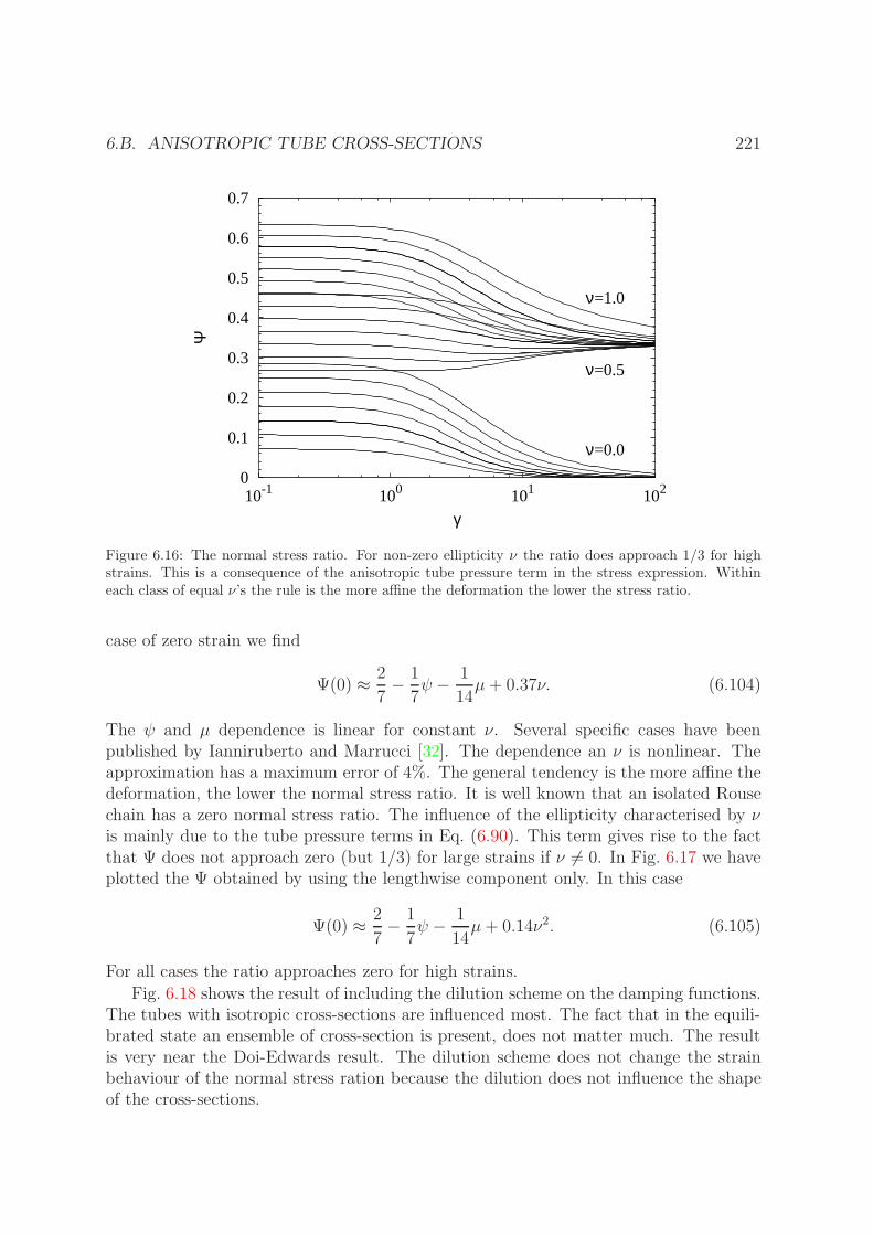
6.B. ANISOTROPIC TUBE CROSS-SECTIONS 221
0
0.1
0.2
0.3
0.4
0.5
0.6
0.7
10-1 100 101 102
Ψ
γ
ν=1.0
ν=0.5
ν=0.0
Figure 6.16: The normal stress ratio. For non-zero ellipticity ν the ratio does approach 1/3 for highstrains. This is a consequence of the anisotropic tube pressure term in the stress expression. Withineach class of equal ν’s the rule is the more affine the deformation the lower the stress ratio.
case of zero strain we find
Ψ(0) ≈ 2
7− 1
7ψ − 1
14µ+ 0.37ν. (6.104)
The ψ and µ dependence is linear for constant ν. Several specific cases have beenpublished by Ianniruberto and Marrucci [32]. The dependence an ν is nonlinear. Theapproximation has a maximum error of 4%. The general tendency is the more affine thedeformation, the lower the normal stress ratio. It is well known that an isolated Rousechain has a zero normal stress ratio. The influence of the ellipticity characterised by νis mainly due to the tube pressure terms in Eq. (6.90). This term gives rise to the factthat Ψ does not approach zero (but 1/3) for large strains if ν 6= 0. In Fig. 6.17 we haveplotted the Ψ obtained by using the lengthwise component only. In this case
Ψ(0) ≈ 2
7− 1
7ψ − 1
14µ+ 0.14ν2. (6.105)
For all cases the ratio approaches zero for high strains.
Fig. 6.18 shows the result of including the dilution scheme on the damping functions.The tubes with isotropic cross-sections are influenced most. The fact that in the equili-brated state an ensemble of cross-section is present, does not matter much. The resultis very near the Doi-Edwards result. The dilution scheme does not change the strainbehaviour of the normal stress ration because the dilution does not influence the shapeof the cross-sections.
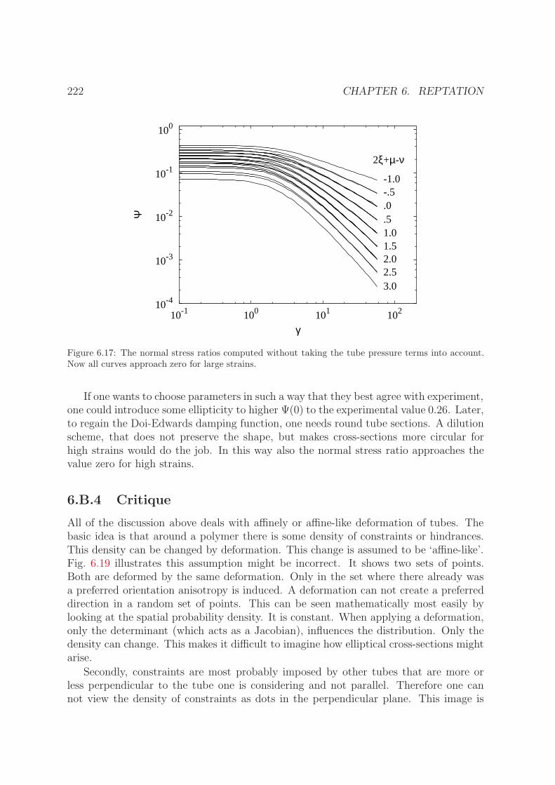
222 CHAPTER 6. REPTATION
10-4
10-3
10-2
10-1
100
10-1 100 101 102
Ψ
γ
2ξ+µ-ν
-1.0-.5.0.51.01.52.02.53.0
Figure 6.17: The normal stress ratios computed without taking the tube pressure terms into account.Now all curves approach zero for large strains.
If one wants to choose parameters in such a way that they best agree with experiment,one could introduce some ellipticity to higher Ψ(0) to the experimental value 0.26. Later,to regain the Doi-Edwards damping function, one needs round tube sections. A dilutionscheme, that does not preserve the shape, but makes cross-sections more circular forhigh strains would do the job. In this way also the normal stress ratio approaches thevalue zero for high strains.
6.B.4 Critique
All of the discussion above deals with affinely or affine-like deformation of tubes. Thebasic idea is that around a polymer there is some density of constraints or hindrances.This density can be changed by deformation. This change is assumed to be ‘affine-like’.Fig. 6.19 illustrates this assumption might be incorrect. It shows two sets of points.Both are deformed by the same deformation. Only in the set where there already wasa preferred orientation anisotropy is induced. A deformation can not create a preferreddirection in a random set of points. This can be seen mathematically most easily bylooking at the spatial probability density. It is constant. When applying a deformation,only the determinant (which acts as a Jacobian), influences the distribution. Only thedensity can change. This makes it difficult to imagine how elliptical cross-sections mightarise.
Secondly, constraints are most probably imposed by other tubes that are more orless perpendicular to the tube one is considering and not parallel. Therefore one cannot view the density of constraints as dots in the perpendicular plane. This image is

6.B. ANISOTROPIC TUBE CROSS-SECTIONS 223
10-3
10-2
10-1
100
100 101 102
h(γ)
γ
µ ν
(0.5, 1.0)(1.0, 0.5)
(1.0, 0.0)(0.0, 1.0)(0.5, 0.5)
(0.5, 0.0)(0.0, 0.5)
(0.0, 0.0)
10-3
10-2
10-1
100
100 101 102
h(γ)
γ
µ ν
(0.5, 1.0)
(0.0, 1.0)(1.0, 0.5)
(0.5, 0.5)
(0.0, 0.5)
(1.0, 0.0)(0.5, 0.0)(0.0, 0.0)
Figure 6.18: The upper graph shows the damping function for ξ = 1 without including the dilutionscheme. In the lower graph the dilution scheme is included. Isotropic cross-sections are influenced most.Their shear thinning curve is very near the Doi-Edwards result.

224 CHAPTER 6. REPTATION
Figure 6.19: Deformation of the left pictures gives the right ones. A deformation can induce ellipticityin a ordered set of points, but not in a random set.

6.C. THE MEAD-LARSON-DOI MODEL 225
implicitly used in the affine deformation hypothesis. On deformation these dots deformaffinely, the density in the other planes changes in a more complicated way. However,because now a whole set of planes has to be considered, this reintroduces the possibilityfor anisotropy to play a role, but in a more complicated way.
6.C The Mead-Larson-Doi model
The one-segment model of Mead, Larson and Doi [18] is an extension on the one-segmentDoi-Edwards equation. It includes convective constraint release and tube stretch. End-effects are not included. Every ensemble of segments is labelled by a time of creation.There is no connection made between position along the tube contour and time ofcreation. The contribution of such an ensemble is described by a survival probabilitydensity µ(t, t′).
The stretch is characterised by a single quantity λ(t). The reptative relaxation ischaracterised by a single relaxation time τd. The rate of convective constraint release,i.e. the rate entanglements disappear is,
k(t) = [κ¯
: S¯− 1
λ(t)
d
dtλ(t)]. (6.106)
This denotes the average rate tube segments stretch minus the rate the chain stretches.It is therefore the rate tube segments are destroyed, which is thought to be equal therate entanglements disappear.
The total rate of relaxation in this model is
1
τ(t)=
1
λ2(t)τd+ f(λ)k(t). (6.107)
The λ2(t) occurs because the time needed to reptate out of the tube increases whenthe tube is longer. The function f(λ) is the so-called switch function which we willdetermine below. Near equilibrium they pose that the stress is proportional to thenumber of entanglements. The decay rate of the stress should therefore equal the rateof constraint release, i.e. f(1) = 1.
For the survival probability density one finds the usual equation
∂
∂tµ(t, t′) = − 1
τ(t)µ(t, t′). (6.108)
The fact that total probability is one results into the rate of creation of new segments
µ(t, t) =1
τ(t). (6.109)
The rate of relaxation of the contour length is given by
d
dtλ(t) = λ(t)κ
¯: S¯− 1
τs(λ(t)− 1)− 1
2k(t)(λ(t)− 1). (6.110)

226 CHAPTER 6. REPTATION
Here τs is the stretch time, which is, at last to within a factor, equal to the Rouse time.The factor 1/2 in front of the rate of constraint release is the same factor 1/2 as inEq. (6.46) and in Eq. (6.55). The origin is tube reorganisation. When 1 segment disap-pears the contour length becomes locally a factor 1/
√2 shorter. Because in equilibrium
λ(t) = 1, the −1 term is introduced. The total stress is given by
τ¯
p =15
4G0λ
2(t)
∫ t
−∞µ(t, t′)dt′ (6.111)
The authors argue, that when constraint release is the only mechanism relaxationmechanism, i.e. reptation and retraction are turned off, and constraints are e.g. manuallyremoved, the stress should relax with a rate k. So, if P (t) is the survival probability forany segment created before t = 0, then
−k(t)λ2(t)P (t) =d
dt[λ2(t)P (t)]
= 2λ(t)P (t)d
dtλ(t) + λ2(t)
d
dtP (t)
= −k(t)λ2(t)P (t) + k(t)[λ(t)− λ2(t)f(λ(t))]P (t),
(6.112)
thus the switch function is
f(λ) =1
λ. (6.113)
This function determines that for slightly stretched chains the convective constraintrelease acts on µ(t, t′), for highly stretched chains it decreases the stretch.

Bibliography
[1] S.F. Edwards. Proc. Phys. Soc., 92:9, 1967.
[2] P.G. de Gennes. J. Chem. Phys., 55:572, 1971.
[3] M. Doi and S.F. Edwards. Dynamics of concentrated polymer systems, part 1.J.C.S. Faraday II, 74:1789–1801, 1978.
[4] M. Doi and S.F. Edwards Dynamics of concentrated polymer systems, part 2. J.C.S.Faraday II, 74:1802–1817, 1978.
[5] M. Doi and S.F. Edwards Dynamics of concentrated polymer systems, part 3. J.C.S.Faraday II, 74:1818, 1978.
[6] G.C. Berry and T.G. Fox. Adv. Polym. Sci., 5:261, 1968.
[7] M. Doi. J. Polym. Sci. (Polym. Phys. Ed.), 21:667, 1983.
[8] S.T. Milner and T.C.B. McLeish. Reptation and contour-length fluctuations inmelts of linear polymers. Phys. Rev. Lett., 81(3):725–728, 1998.
[9] J. des Cloizeaux. Relaxation of entangled polymers in melts. Macromolecules,23:3992–4006, 1990.
[10] S.T. Milner. Relating the shear-thinning curve to the molecular weight distributionin linear polymer melts. J. Rheology, 40(2):303–315, 1996.
[11] G. Marrucci. Dynamics of entanglements: A nonlinear model consistent with theCox-Merz rule. J. Non-Newtonian Fluid Mech., 62:279–289, 1996.
[12] S.T. Milner, T.C.B. McLeish, R.N. Young, A. Hakiki, and J.M. Johnson. Dynamicdilution, constraint-release, and star-linear blends. Macromolecules, 31(26):9345–9353, 1998.
[13] S.T. Milner and T.C.B. McLeish. Arm-length dependence of stress relaxation instar polymer melts. Macromolecules, 31(21):7479–7482, 1998.
[14] M.A. Hulsen, A.P.G. van Heel, and B.H.A.A. van den Brule. Simulation of vis-coelastic flows using brownian configuration fields. J. Non-Newtonian Fluid Mech.,70(1-2):79–101, 1997.
227

228 BIBLIOGRAPHY
[15] G. Ianniruberto and G. Marrucci. Stress tensor and stress-optical law in entangledpolymers. J. Non-Newtonian Fluid Mech., 79:225–234, 1998.
[16] K. Osaki, K. Nishizawa, and M. Kurata. Macromolecules, 15:1068, 1982.
[17] C.C. Hua, Schieber J.D. and D.C. Venerus. Segment connectivity, chain-lengthbreathing, segmental stretch, and constraint release in reptation models. III. Shearflows. J. Rheology, 43(3):701–717, 1999.
[18] D.W. Mead, R.G. Larson, and M. Doi. A molecular theory for fast flows of entangledpolymers. Macromolecules, 31(22):7895–7995, 1998.
[19] G. Marrucci and G. Ianniruberto. Open problems in tube models for concentratedpolymers. J. Non-Newtonian Fluid Mech., 82:275–286, 1999.
[20] M. Doi and S.F. Edwards. The theory of polymer dynamics. International series ofmonographs on physics, no. 73. Clarendon, Oxford, 1986.
[21] M. Doi. Stress relaxation of polymeric liquids after double step strain. J. Polym.Sci. (Polym. Phys. Ed.), 18:1891–1905, 1980.
[22] G. Ianniruberto and G. Marrucci. On compatibility of the Cox-Merz rule with themodel of Doi-Edwards. J. Non-Newtonian Fluid Mech., 65:241–246, 1996.
[23] C.C. Hua and J.D. Schieber Segment connectivity, chain-length breathing, seg-mental stretch, and constraint release in reptation models. I. theory and single-stepstrain predictions. J. Chem. Phys., 109(22):10018–10027, 1998.
[24] C.C. Hua, Schieber J.D. and D.C. Venerus. Segment connectivity, chain-lengthbreathing, segmental stretch, and constraint release in reptation models. II. double-step strain predictions. J. Chem. Phys., 109(22):10028–10032, 1998.
[25] G. Marrucci, F. Greco, and G. Ianniruberto. Possible role of force balance onentanglements. to be published in Macromol. Symp., 2000.
[26] G. Marrucci, F. Greco, and G. Ianniruberto. Integral and differential constitutiveequations for entangled polymers with simple versions of CCR and force balanceon entanglements. to be published in Rheol. Acta.
[27] R.C. Ball and T.C.B. McLeish. Dynamic dilution and the viscosity of star polymermelts. Macromolecules, 22:1911–1913, 1989.
[28] G. Marrucci. Relaxation by reptation and tube enlargement: a model for polydis-perse polymers. J. Polym. Sci. (Polym. Phys. Ed.), 23:159–177, 1985.
[29] J.L. Viovy, M. Rubinstein and R.H. Colby. Constraint release in polymer melts:tube reorganisation versus tube dilution. Macromolecules, 24:3587–3596, 1991.
BIBLIOGRAPHY 229
[30] G. Marrucci and B. de Cindio. The stress relaxation of molten pmma at largedeformations and its theoretical interpretation. Rheo. Acta, 19:68–75, 1980.
[31] G. Marrucci and G. Ianniruberto. Polymeric liquids at high shear rates. In M.J.Adams, R.A. Mashelkar, R.A. Pearson and A.R. Rennie, editors, Dynamics of com-plex fluids, pages 176–187. Imperial College Press-The Royal Society, 1998.
[32] G. Marrucci, F. Greco and G. Ianniruberto. Rheology of polymer melts and con-centrated solutions. Curr. Opin. Colloid Interface Sci., 4(4):283–287, 1999.
[33] M.H. Wagner and J. Schaeffer. Nonlinear strain measures for biaxial extension ofpolymer melts. J. Rheology, 36(1):1–26, 1992.
[34] H.C. Ottinger. Thermodynamically admissible reptation models with anisotropictube cross sections and convective constraint release. J. Non-Newtonian FluidMech., 89:165–185, 2000.
[35] R.B. Bird, C.F. Curtiss, R.C. Armstrong and O. Hassager. Dynamics of PolymerLiquids. Vol. 2. Kinetic Theory. John Wiley, New York, 2 edition, 1987.

230 BIBLIOGRAPHY

Chapter 7
The deformation fields method∗
7.1 Introduction
In this chapter we are not concerned with the physics of constitutive equations. Ourconcern will be the macroscopic flow of liquids whose behaviour is governed by theseequations. The special class of constitutive equations for the stress considered here is theclass of integral constitutive equations. The flow will be taken to be incompressible andisothermal. In the analysis of a viscoelastic fluid flowing through a complex domain oneusually has to resort to a numerical simulation of the problem. The deformation fieldsapproach is a method to incorporate integral constitutive equations into macroscopicflow simulations.
In most numerical studies the constitutive model is of a differential type, in whichthe stress tensor evolves via a differential equation. In these kind of equations the rate-of-deformation tensor is used as an input. Differential constitutive equations have thenumerical advantage that the evolution of the stress at a certain instance in time dependson the current velocity and stress fields only. Using a differential constitutive equationtherefore has the clear advantage that it is not necessary to store the complete historyof the flow problem.
On the other hand, many (potentially) successful constitutive models are not ofa differential type. These constitutive equations include the kinetic micro-rheologicalmodels and also integral models. Some of the more successful constitutive models todescribe the behaviour of a polymer melt, such as the equations following from reptationtheory, are of the integral type. In recent years there is a trend to incorporate thesesophisticated models directly into the simulation of the flow of a macro-molecular fluid,without resorting to an approximation by a differential type model.
To evaluate a flow problem using an integral constitutive equation, it seems mostnatural to use a Lagrangian description of the flow field; the memory integral can beevaluated relatively easy by following the fluid particle. The main drawback of thisapproach is that in a Lagrangian description the computational mesh deforms with thefluid. In a strong flow field this means that regular re-meshing is required to maintain
∗Parts of this chapter have appeared in two publications [1] and [2].
231

232 CHAPTER 7. THE DEFORMATION FIELDS METHOD
numerical accuracy. This is not only cumbersome but also leads to a loss of accuracysince in the re-meshing procedure one has to interpolate the solution on the old meshin order to find the values of the relevant variables at the nodal points of the newmesh. Another less attractive element of a Lagrangian implementation is that, in orderto achieve a refinement of the mesh somewhere in a problematic area downstream inthe flow field, one already has to know upstream how to construct the mesh. A goodexample of a Lagrangian approach to viscoelastic flow modelling can be found in thepapers by Rasmussen & Hassager [3] and [4].
In a Eulerian approach all the problems associated with the deformation of themesh are of course absent. The deformation fields method is a time dependent Eule-rian technique for implementing integral constitutive equations, bypassing the problemsassociated with mesh deformation without being limited to steady state problems.
As will be discussed in §7.2 the step from Lagrangian, i.e. tracking fluid particles, toEulerian methods is related to the same step that was made earlier for kinetic modelsgiving rise to the Brownian configuration field method. The step from a Lagrangian ap-proach to A Eulerian one is generally established by the introduction of fields. One canthink more abstractly of deformation (and configuration) fields as containing informationneeded to calculate the stress. Instead of tracking fluid particles the information con-tained in the fields is convected with the fluid flow. In the configuration field method theinformation contained in the fields is information on polymer configuration. In the defor-mation fields method the fields store Finger tensors. These characterise the deformationof a fluid particle with respect to some reference time in the past. In Rivlin-Sawyersequations the stress is an integral of a function of these Finger tensors with respect tothis reference time.
Kinetic theories describe the evolution of the polymer configuration. In many models,including network models and reptation models, configurational information can be eas-ily obtained from information on the deformation history as contained in Finger tensors.Now instead of simulating the configurational changes one can simulate the deformationhistory using the deformation fields approach. The step from deformational informa-tion to configurational information is only made when performing the stress calculation.In this way the deformation fields approach can be used for many models obtained bykinetic modelling.
A good example of this procedure can be found in van Heel et al. [5]. Here the Doi-Edwards model is first simulated using configurational information only (the orientationof tube segments). The second approach utilises deformational information (deformationgradient tensors in this case). The deformational information can be used to obtain theconfiguration of tube segments starting from an isotropic distribution. The stress isthen obtained by an averaging procedure using this equilibrium ensemble. In §7.7 it willbe shown that making the step to configurational information so explicitly is actuallynot necessary here. The results of Van Heel et al. show that for the Doi-Edwardscase the deformation fields approach is much more efficient than the configuration fieldsapproach.
Many recently proposed models for polymer melt flow are of a mixed character. In

7.2. LITERATURE 233
these models the orientational information of polymer segments is treated separatelyfrom other configurational information such as chain stretch. The contribution to thestress from orientational effects can then be determined by using deformation fields. Theother configurational information is stored in extra configuration fields. Two models thathave such form are the pom-pom model [6], [7] and the Mead-Larson-Doi [8] model (see§7.8.2). The reptation models developed in the previous chapter also fall in this category.
After a short discussion on related topics in literature we will start discussing ournumerical method for macroscopic flow simulations of viscoelastic fluids. The basic de-formation fields method, as needed for incorporating Rivlin-Sawyers integral constitutiveequations into flow calculations, will be treated first. Both the general ideas and somedetails of the current implementation will be discussed. The simulation of the consti-tutive equation for the stress is only one aspect of a viscoelastic flow simulation. Theother one is solving the balance equations (for mass and momentum). The simulationof viscoelastic flow is a highly specialised branch of research, which has made a lot ofprogress the last decades. It was realised that viscoelastic fluids need very specialisedmethods. We will give a short overview of methods that are used in our computations.
At this point all ingredients, needed to perform flow calculation using Rivlin-Sawyersintegral equations, are present. We will show flow simulations of a sphere moving in atube filled with visco elastic fluid. The model used in the computation is the integralformulation of the upper-convected Maxwell equation. This is a well known benchmark-ing problem. The simulations are compared with results from literature, which wereobtained by different methods. We will also demonstrate one of the benefits of the de-formation fields method namely the use of a broad spectrum of relaxation times. Forthis means the Rouse model is used.
Then we proceed with Rivlin-Sawyers models using non-linear measures of strain.An example of a model with a non-linear strain dependence is the PSM-model, but alsosimple reptation models, like the Doi-Edwards model, fall in this category. A simulationusing the PSM-model will be presented. The results are compared with those obtainedby Rasmussen and Hassager [9].
Already in the treatment of non-linear strain measures the use of the deformationfields method for simulating kinetic models, such the Doi-Edwards reptation model,becomes clear. Next we will discuss extensions to the basic scheme of the method, neededto simulate more advanced reptation models such as the Mead-Larson-Doi model, thepom-pom model or the reptation model discussed in the previous section. These methodswill be illustrated by the presentation of simulation results generated using the Mead-Larson-Doi model.
7.2 Literature
The deformation fields method as presented in this chapter is related to many differentmethods in computational rheology. First of all it is a method to numerically solveflow problems when integral constitutive equations are used to model the dependenceof the stress on the deformation history. The commonly used strategy to incorporate
234 CHAPTER 7. THE DEFORMATION FIELDS METHOD
integral equations in flow calculations is to integrate backwards along the trajectory offluid particles. The stress at a point in space is a function of the deformation historyof that fluid particle. In stationary flow the particle trajectories do not change in time.Here the trajectories coincide with streamlines. The information needed to calculatethe stress in a fluid particle consists of the velocity and the velocity gradient whenmoving upstream along a streamline. All deformational information needed to computethe stress is thus contained in one velocity field. Methods for incorporating integralequations in stationary flows are called streamline integration methods. Examples ofresults obtained by these methods can be found in [10], [11] and [12]. The streamlineintegration method is difficult to generalise to non-stationary flow. To our knowledgenobody has ever tried this.
The deformation fields approach is especially designed for instationary situations.Here all the information that is needed is no longer contained in one flow field. To storethe information many new fields, the deformation fields are introduced. In the defor-mation fields method no tracking is needed because the fields themselves are convectedwith the flow.
Intuitively co-moving with fluid particles is the more natural way of thinking aboutdeformation histories. Methods in which the mesh is co-moving and co-deforming withthe flow are called Lagrangian (as opposed to Eulerian where the mesh is not deformed).As mentioned in the introduction these methods have some drawbacks that have to dowith re-meshing and mesh refinement. Nevertheless Rasmussen and Hassager showedthat a Lagrangian method can be used for doing instationary simulations with integralmodels. In the first two papers [3] and [4] they use an upper-convected Maxwell model(UCM) to model the flow past a sphere falling along the centreline of cylindrical tube.Because the UCM model can be expressed in a differential form it is, in principle,not necessary to store the complete deformation history. In a later paper [9] they usethe Papanastasiou-Scriven-Macosko model (PSM) which is a member of the Rivlin-Sawyers class of equations. This equation does not have an differential analogue. In thesimulation with this model all the previous coordinates of the deforming mesh have tobe stored in order to be able to reconstruct the deformation history. In §7.7.1 we makea comparison with these simulation results.
On a conceptual and computational level the deformation fields method is relatedto the Brownian configuration field method. This method was introduced to efficientlyincorporate a kinetic model into a flow simulation, bypassing the need for a closed-formconstitutive equation. The ‘CONNFFESSIT’ approach (calculation of non-Newtonianflow: finite elements and stochastic simulation technique) developed by Laso and Ottinger[13] was the first step for establishing such a coupling of methods. Their original methodwas a particle tracking method with uncorrelated stochastic processes acting on eachparticle [14]. A Eulerian approach to incorporate Brownian dynamics simulations in aviscoelastic flow simulation was developed by Hulsen, van Heel & van den Brule [15]. Inthis method the molecular orientations are stored in an ensemble of configuration fields.The stochastic process is taken to be the same everywhere within a configuration fieldwhile the noise in different fields remains uncorrelated. In this way spatial derivatives
7.3. THE FINGER TENSOR 235
are smooth in contrast to the CONNFFESSIT method. This is especially importantfor the computation of the divergence of the stress tensor that is needed for solving thebalance equations.
Historically the development of the deformation fields method started out as an at-tempt to model a certain class of equations using the configuration fields approach. Theequations concerned are the stochastic equations proposed by Feigl and Ottinger [16],[17], which describe affine deformation of a vector and a surface element (characterisedby a perpendicular vector). These two vectors can be created from an isotropic initialdistribution and subsequently annihilated according to a lifetime distribution. This is theclassical setting of network theory. When polymer strands are temporarily crosslinkedthey co-deform with the bulk (i.e. move affinely). When a crosslink or an entanglementdisappears the strand re-equilibrates.
Feigl and Ottinger show that the equations are equivalent to time-separable Rivlin-Sawyers equations. They also give the procedure for going from the stochastic descrip-tion to the Rivlin-Sawyers description and back. When trying to develop a method tosimulate the stochastic equations using configuration fields it quickly became clear tous that simulations using the Rivlin-Sawyers formulation are much cheaper. Then thedeformation fields approach was developed.
The important point of the Feigl-Ottinger papers is that modelling using the stochas-tic approach is much closer to the physics than the Rivlin-Sawyers approach, and thusmight be more successful in the long run. Although we think this is probably true, it iswise to translate a successful stochastic network theory into an integral formulation, ifpossible, when doing flow calculations.
7.3 The Finger tensor
In section §7.5 we will treat the problem of numerically solving viscoelastic flow problems.The solution of this problem consists of solving the balance equations of mass andmomentum. To get a closed set of equations the stress tensor has to be provided.A constitutive equation for the stress relates the deformation history of a polymericmaterial to the stress. Finger tensors characterise the deformation of the material. Theyare the main quantity in the integral equations we will be considering in this chapter.
In the continuum approach to viscoelastic modelling it is often assumed that thestress in a fluid particle is a function of the deformation history of that fluid particle.This is the assumption of locality. In reality, polymers in neighbouring fluid elementsdo have some centre of mass diffusion. Therefore information on deformation historiesdoes diffuse from one fluid particle to another. This effect is assumed to be negligible.
The deformation history of a fluid particle at time t is fully characterised by the setof deformation gradient tensors F
¯t′(t), for all t′ < t. Here t′ denotes a reference time.
An infinitesimal line element ∆x¯
t′ at time t′ is deformed to ∆x¯
t at time t via
∆x¯
t = F¯
t′(t) ·∆x¯
t′ . (7.1)

236 CHAPTER 7. THE DEFORMATION FIELDS METHOD
The time evolution of F¯
t′(t) with the reference time t′ fixed is
D
DtF¯
t′(t) = ∇u¯
T (t) · F¯
t′(t). (7.2)
The deformation from a time t1 to a later time t2 (t1 < t2 < t) can be inferred from thisto be
F¯
t1(t2) = F¯
t1(t) · F¯−1t2 (t), (7.3)
confirming that the set F¯
t′(t) indeed characterises the whole deformation history upto the current time.
The Finger tensor, B¯
t′(t), is related to the deformation gradient tensor by
B¯
t′(t) = F¯
t′(t) · F¯
Tt′ (t). (7.4)
This tensor characterises affine deformation of a (imaginary) fluid particle that wasspherical (isotropic) at time t′. A powerful result of continuum mechanics is that for anymaterial, satisfying some mild conditions, the stress can be expressed as a functional ofthe Finger tensors [18],
τ¯(t) = F [B
¯t′(t)]
tt′=−∞. (7.5)
The most demanding of the conditions is called objectivity or material indifference. Thisessentially requires that inertial effects (or more precisely angular momentum effects)play no role in the dynamics of the micro structure. A second is that the materialproperties have to be isotropic at equilibrium. The last demand is incompressibility. Ifthis is not satisfied, an extra variable, namely the density is needed.
To further narrow down the class extra modelling assumption have to be made. Aparticular set of these assumptions results in the integral equations that will be treatedin the next section. The Finger tensor fields are the primary variables in these equations.This is the quantity that has to be updated and convected with the flow such that thestress can be calculated. They are stored in the deformation fields. The time evolutionof the Finger tensor B
¯t′(t) is governed by
B¯
5t′ = 0
¯, (7.6)
or
∂
∂tB¯
t′(x¯, t) + v
¯(x¯, t) · ∇B
¯t′(x
¯, t)
= ∇u¯
T (x¯, t) · B
¯t′(x
¯, t) +B
¯t′(x
¯, t) · ∇u
¯(x¯, t), (7.7)
where one should keep in mind that t′ is a reference time that should be kept fixed.At every instant in time a Finger tensor field is created (as a unit tensor). For this
new tensor the present time equals the reference time, i.e. t = t′. The fact that B¯
t′(t′) = δ
¯

7.4. INTEGRAL EQUATIONS 237
is immediately clear from Eq. (7.1) (combined with Eq. (7.4)). The unit tensor is theinitial condition for the evolution equation for the Finger tensor field Eq. (7.7).
Thus after creation, the field is deformed and convected by the flow, obeying Eq. (7.7).The second term on the LHS of Eq. (7.7) accounts for the convective motion of thefield. To effectively handle this term in the flow computation the discontinuous Galerkindiscretisation is used in the finite element implementation of the deformation fields, see§7.5. The convective term removes the need to track the motion of fluid particles.
The terms on the RHS of Eq. (7.7) describe the further deformation of the field causedby the presence of a velocity gradient. The important thing to notice in Eq. (7.7),and the key of our approach, is that the evaluation of the time evolution of B
¯t′(x
¯, t)
only requires information of the velocity field at the current time t. All informationabout the flow history is contained in the Finger tensors B
¯t′(x
¯, t) with t′ < t. In the
actual implementation not the full tensors are stored and updated, but the number ofcomponents is reduced by one. This is accomplished by using the fact that det(B
¯t′) = 1.
The details are given in Appendix 7.A. Apart from reducing the storage and CPUrequirements there also seems to be a slight improvement in accuracy, but further studyis needed to give a more definite statement on this.
For the time discretisation of the evolution equation Eq. (7.7) we use an explicit
Euler scheme. Therefore, the Finger tensor at the next time step B¯
(n+1)t′ is computed
from the velocity and the Finger tensor at the current time as follows
B¯
(n+1)t′ = B
¯(n)t′ + ∆t[−u
¯(n) · ∇B
¯(n)t′ + (∇u
¯(n))T · B
¯(n)t′ +B
¯(n)t′ · ∇u¯
(n)], (7.8)
where we omitted the dependence on x¯.
Having the Finger tensor fields at hand (for all t′) the stress tensor can be calculated.The constitutive equation we use here is the integral constitutive equation and will betreated below. It is of course impossible to know the Finger tensor fields for all t′.Therefore the reference time t′ has also to be discretised. This problem will be addressedin §7.4.2.
7.4 Integral equations
7.4.1 Time-Separable Rivlin-Sawyers equations
For the time-separable Rivlin-Sawyers model the stress tensor is given by the followingrelation
τ¯
p(x¯, t) =
∫ t
−∞M(t− t′)f
¯[B¯
t′(x¯, t)]dt′, (7.9)
where M(t) is the memory function and f¯[] an isotropic tensor function. This integral
is the stress calculator which relates the Finger tensor fields to the stress tensor. In thissection we will discuss some physical issues related to the use of these equations. Thenext sections will be concerned with the numerical implementation.

238 CHAPTER 7. THE DEFORMATION FIELDS METHOD
From a kinetic theory point of view these equations are easiest understood to ariseas ‘network’ models. At time t′ a polymer strand forms a non-permanent crosslink witha polymer network. This strand has no preferred orientation. The strand deforms withthe network which itself deforms with the flow (i.e. affinely). This process halts whenthe strand detaches. The probability a strand created at time t′ is still attached at timet is proportional to M(t− t′). Therefore M(t− t′) is a weighting factor of an ensemble ofstrands created at t′. The contribution of such an ensemble to the stress is f
¯[B¯
t′ ]. Thiskind of interpretation can also be made for some other models than network models, e.g.the independent alignment Doi-Edwards model. Here the primary quantities are tubesegments that rotate affinely, see previous chapter.
Besides theoretical reasons the use of time-separable Rivlin-Sawyers equations hasexperimental motivations. The model has free parameters that can be related to exper-imental data in a simple way. The function f
¯[B¯] fully characterises the initial response
to a rapid step strain deformation. It is often called a measure of strain, or in reptationtheory the Q-tensor. It is discussed more elaborately in §7.7. An experimentally verywell documented step strain quantity is the damping function, h(γ). This function char-acterises the initial response to a shear strain γ (τxy = G0h(γ)γ). For two dimensionalflow this damping function fully characterises the Q-tensor.
A second experimental characterisation is linear viscoelastic response. Here the strainis small and B
¯t′(t) can be approximated by δ
¯+ γ
¯t′(t), which gives
τ¯
p(t) =
∫ t
−∞M(t− t′′)γ
¯t′′(t)dt
′′
=
∫ t
−∞M(t− t′′) [
∫ t
t′′γ¯(t′)dt′]dt′′
=
∫ t
−∞[
∫ ∞
t−t′M(τ)dτ ]γ
¯(t′)dt′,
(7.10)
(the constant isotropic contribution is not considered because it can be incorporated intothe pressure). Comparing this with the Boltzmann superposition for linear viscoelasticresponse
τ¯
p(t) =
∫ t
−∞G(t− t′)γ
¯(t′)dt′ (7.11)
gives that the memory function can be related to the relaxation modulus G(τ) via thesimple relation
M(τ) = − d
dτG(τ). (7.12)
The relaxation modulus G(t) can be measured using standard rheological techniques.We can conclude that the functions needed to specify a time-separable Rivlin-Sawyers
equations for a specific liquid can be inferred from experiment. In that case, both thelinear viscoelastic response and the initial response to a step strain predicted by the

7.4. INTEGRAL EQUATIONS 239
equation will be in agreement with experiment. For the Rivlin-Sawyers equation to bea satisfactory constitutive equation it has to be able to predict other flow phenomena.The first obvious test is relaxation subsequent to a sudden response. According to thetime-separable Rivlin-Sawyers equation this response should have the form h(γ)M(t).This means that by rescaling the response as a master curve M(t) is to be found. Thefunction h(γ) is the rescaling factor. As discussed in §6.2 for melts this is found tobe true when considering large enough times. Large enough means, in this case, timescales where re-orientation of tube segments is the dominant mechanics and not stretchrelaxation. Therefore if the characteristic time in the flow is smaller then the timecorresponding with stretch, strain-time-separability is a valid assumption.
The other obvious quantity to look at is shear-rate dependence of the stationaryshear viscosity. If in a Rivlin-Sawyers equation the experimental damping function andrelaxation modulus are used, the stationary shear is found to be much more shear thin-ning than observed in experiments. The current explanation is that there are relaxationmechanisms (convective constraint release) related to (fast) flow, see appendix 6.A.
Both stretch and convective constraint release is modelled in the Mead-Larson-Doimodel (see appendix 6.C). This model thereby differs from an ordinary time-separableRivlin-Sawyers equation. It can however be simulated by the deformation fields method.To simulate stretch an extra configurational field (namely the stretch parameter λ) hasto be simulated, see §7.8.1. To incorporate the convective constraint release mechanism,relaxation times have to be made flow dependent. This leads to the introduction of extra‘weight fields’ (one for every t′), see §7.8. These kind of extensions make the deformationfields method very powerful.
7.4.2 The discretisation of the reference time
The contribution of a particular field to the stress at the current time t is weighted bythe memory function and depends on the age of the field, i.e. t − t′. To construct thememory integral one would ideally like to know f
¯[B¯
t′(x¯, t)] for all t′. To approximate this
infinite amount of information, f¯[B¯
t′ ] will be discretised with respect to the referencetime t′. Furthermore, a cutoff time τc is introduced by limiting the reference time tot − τc < t′ < t. To reconstruct the discretised version of f
¯[B¯
t′ ], the tensor fields B¯
t′
only have to be stored for a finite number of reference times t′. In this way we obtaina manageable number of fields, the deformation fields, each labelled by their time ofcreation.
The functions f¯[B¯
t′ ] for a continuous t′ are approximated by means of an interpola-tion between the discrete fields created at times t− τi in the past. For this reason linearbase functions φi(τ) are introduced (see Fig. 7.1),
f¯[B¯
t−τ (t)] =
N−1∑i=0
f¯[B¯
t−τi(t)]φi(τ). (7.13)
As can be seen in Fig. 7.1 a special choice is made for the last base function. This is anespecially good choice in startup problems. In startup problems (with startup at t = 0)

240 CHAPTER 7. THE DEFORMATION FIELDS METHOD
M()4()
1 2 4 5 6 c730
Figure 7.1: The tensors f¯[B¯ t−τ (t)] are only known for discrete ages τi. For intermediate ages we use
the base function φi(τ) to make an interpolation: f¯[B¯ t−τ (t)]=
∑i f¯[B¯ t−τi(t)]φi(τ). In this figure we
depicted the base functions used in our case (linear interpolation).
all B¯
t′ with t′ < 0 are equal. The choice of taking the base function to be 1 for τ > τcmakes that there is no cutoff error for times t < τc. Substitution of the expression intoEq. (7.9) yields
τ¯
p(x¯, t) =
∑i
Wif¯[B¯
t−τi(x¯, t)], (7.14)
where the weights Wi are given by
Wi =
∫ ∞
0
M(τ)φi(τ)dτ. (7.15)
The weights Wi only have to be calculated once, before the start of the actual flowsimulation. The stress integral is approximated by a finite sum and is second-order intime. If f
¯[B¯
t′ ] is bounded and τc is of the order of a few times the largest relaxationtime, the error due to this truncation will be relatively small since most realistic memoryfunctions decay exponentially for large times. There are models where f
¯[] is not bounded,
e.g. the Maxwell or Rouse model. The stress in these models can diverge in a strongelongational flow. The errors due to truncation of the memory function can underthese circumstances become very large. The possibility to grow without bound indicatesa serious flaw in the constitutive equation. For the Rouse chain e.g. the underlyingproblem is the infinite extensibility at large but finite rates of elongation.
Old fields will contribute very little to the stress since the memory function is adecreasing function of time. Therefore a cutoff time τc is introduced, as explained in theprevious paragraph. This also offers the possibility to, every time step, annihilate an oldfield. In this way memory space is created to store the newly created field which carriesthe current time as a label. Using this procedure the number of fields is kept constantduring the simulation.
To keep things clear, we will first present the simplest approach to the implementationof deformation fields. The time discretisation of the deformation fields will be taken tobe equidistant and we will use the same time increment ∆t as the one used in the flowsimulation to solve the balance equations. The update algorithm of the deformationfields consists of three steps:

7.4. INTEGRAL EQUATIONS 241
weight update t+tt
W3
W4
W5
W6
WN1
W2
Btt(~x; t)
Bt+t(~x; t+t) = 1
Bt2t(~x; t)
Bt3t(~x; t)
Bt4t(~x; t)
Bt5t(~x; t)
Bt6t(~x; t)
W1
W0
Btt(~x; t+t)
Bt2t(~x; t+t)
Bt3t(~x; t+t)
Bt4t(~x; t+t)
Bt5t(~x; t+t)
Bt6t(~x; t+t; t)
Btc(~x; t)
NULL
Bt(~x; t)
Bt(~x; t+t)
Figure 7.2: The infinite number of fields B¯ t′(x¯
, t) is represented by a finite number of fields. This isdone by introducing a cut-off time, and by discretising the integral.
• Updating of the existing fields, i.e. the convection and deformation of the memoryfields.
B¯
t−i∆t(t)→ B¯
t−i∆t(t+ ∆t) (7.16)
• Annihilation of an old field. In the simple approach, equidistant discretisation, theoldest field will be annihilated.
B¯
t−τc(t)→ NULL (7.17)
• Creation of a new field. Using the memory space released by annihilation of anold field a new field is created as a unit tensor field with reference time t+ ∆t.
B¯
t+∆t(t+ ∆t) := 1¯
(7.18)
In addition to the updating of the fields the weights associated to each field have to bedecreased since they aged by a time increment. The field B
¯t−i∆t(t) was i time steps old
and therefore f¯[B¯
t−i∆t(t)] attributes with weight Wi to stress tensor. The updated fieldis i + 1 time steps old and has a new, and lower, weight Wi+1. This is illustrated inFig. 7.2. Using the new weights, the stress throughout the flow domain can be calculated.With the new stresses the velocity field can be updated etc..
Since the time step for the evaluation of the memory integral has to obey othercriteria than the time step used for solving the momentum balance and the update of
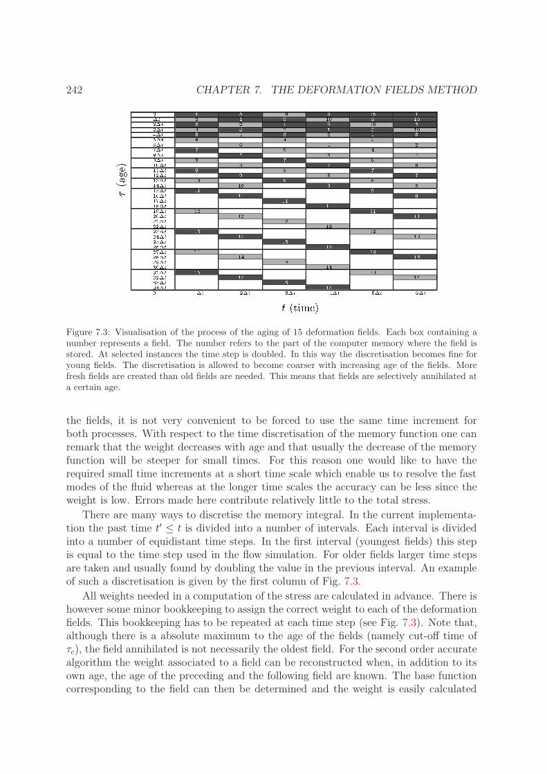
242 CHAPTER 7. THE DEFORMATION FIELDS METHOD
t (time)
(age)
1
1
1
1
2
2
2
2
3
14
3
3
4
45
6
7
8
9
10
11
12
13
14
15
11
11
11
12
12
12
13
13
13
14
14
14
15
15
15
15
15
14
13
13
12
12
11
11
10
10
9
9
9
9
9
8
8
8
8
7
7
7
7
7
6
6
6
6
5
5
5
5
4
3
10 3
10
10
3
4
4
2
2
4
t 2t 3t 4t 5t
0
2t
t
3t
4t
5t
6t
7t
8t
9t
10t
11t
12t
13t
14t
15t
16t
17t
18t
19t
20t
30t
31t
32t
33t
34t
21t
22t
23t
24t
25t
26t
27t
28t
29t
0
51
8
6
1
6t
Figure 7.3: Visualisation of the process of the aging of 15 deformation fields. Each box containing anumber represents a field. The number refers to the part of the computer memory where the field isstored. At selected instances the time step is doubled. In this way the discretisation becomes fine foryoung fields. The discretisation is allowed to become coarser with increasing age of the fields. Morefresh fields are created than old fields are needed. This means that fields are selectively annihilated ata certain age.
the fields, it is not very convenient to be forced to use the same time increment forboth processes. With respect to the time discretisation of the memory function one canremark that the weight decreases with age and that usually the decrease of the memoryfunction will be steeper for small times. For this reason one would like to have therequired small time increments at a short time scale which enable us to resolve the fastmodes of the fluid whereas at the longer time scales the accuracy can be less since theweight is low. Errors made here contribute relatively little to the total stress.
There are many ways to discretise the memory integral. In the current implementa-tion the past time t′ ≤ t is divided into a number of intervals. Each interval is dividedinto a number of equidistant time steps. In the first interval (youngest fields) this stepis equal to the time step used in the flow simulation. For older fields larger time stepsare taken and usually found by doubling the value in the previous interval. An exampleof such a discretisation is given by the first column of Fig. 7.3.
All weights needed in a computation of the stress are calculated in advance. There ishowever some minor bookkeeping to assign the correct weight to each of the deformationfields. This bookkeeping has to be repeated at each time step (see Fig. 7.3). Note that,although there is a absolute maximum to the age of the fields (namely cut-off time ofτc), the field annihilated is not necessarily the oldest field. For the second order accuratealgorithm the weight associated to a field can be reconstructed when, in addition to itsown age, the age of the preceding and the following field are known. The base functioncorresponding to the field can then be determined and the weight is easily calculated

7.5. VISCOELASTIC FLOW SIMULATIONS 243
using Eq. (7.15).We found that about 100 deformation fields were sufficient to represent the defor-
mation history with a high accuracy. The optimal distribution of the time intervals candiffer slightly for different memory functions.
7.5 Viscoelastic flow simulations
7.5.1 Balance equations
The problem considered in this chapter is that of isothermal flow of a viscoelastic fluid ina complex domain. The fluid is assumed to be incompressible. The continuity equationfor mass therefore reduces to
∇ · u¯(x¯, t) = 0, (7.19)
where u¯(x¯, t) is the velocity field. Furthermore it is assumed that inertial effects are
negligible. Under these assumptions the flow is governed by the momentum balancewhich reduces to
∇ · σ¯(x¯, t) = ∇ · τ
¯(x¯, t)−∇p(x
¯, t)
= ηs∇2u¯(x¯, t) +∇ · τ
¯p(x
¯, t)−∇p(x
¯, t) = 0.
(7.20)
Because inertia is neglected the macroscopic momentum itself plays no role in the mo-mentum balance (i.e. creeping flow). On every fluid element there is a force balance ofsurface forces expressed by the stress tensor. The total stress σ
¯has two contributions:
the extra stress τ¯
which is governed by the constitutive equation of the model and anisotropic pressure contribution −pδ
¯. The pressure is not an independent variable but has
to be taken such that the incompressibility condition is enforced. It can be thought of asa Lagrange multiplier for the constraint condition of divergence free flow. Often the fluidstress is decomposed into two parts: a viscous Newtonian solvent part ηs(∇u
¯+ ∇u
¯T )
and a viscoelastic stress τ¯
p. In order to close the set of equations, a constitutive relationis needed which expresses the polymer stress τ
¯p in terms of the history of deformation.
The Rivlin-Sawyers constitutive equation as treated in the previous section is an exam-ple of such an equation. In this section we will treat the numerical techniques to couplethe constitutive equation into the balance equations and solve them numerically.
The equation Eq. (7.20) is highly implicit. At every time the total stress has to be di-vergence free. The change of the stress in a specific point in space has two contributions.Firstly stress is convected from a neighbouring element. This is a very important contri-bution because of the large memory effects of viscoelastic fluids. Secondly the stress of afluid particle evolves. The reason for this is that the underlying micro structure evolves.There are two aspects to this evolution namely deformation by flow and equilibrationby thermal motion. The way the stress changes when applying a certain deformationdepends on the instantaneous micro structure. And this micro structure depends itselfagain on the whole deformation history. The task one wants to perform when doing

244 CHAPTER 7. THE DEFORMATION FIELDS METHOD
a flow simulation is to find the time evolution of a flow field, such that a divergencefree stress field is maintained in the convected and deformed material, everywhere andalways.
7.5.2 The time stepping procedure
As was outlined at the end of the previous section, solving the creeping flow equationfor viscoelastic liquids is a highly implicit problem. To solve this problem numericallyone might think of reintroducing a small density and include inertia effects in Eq. (7.20).This then would give an expression for the acceleration which can be used to update theflow field. First of all, we are here not especially interested in inertial effects. Secondly toobtain stable results this method would require very small time steps. If one neverthelesswants to include inertial effects for (near) creeping flow the common procedure is tomodel the macroscopic momentum contribution as a source term in the equation forsolving the momentum equation.
The strategy actually used for solving creeping flow of viscoelastic fluids is largelybased on approaches developed to simulate Stokes flow. In solving Stokes flow the lineardependence of the stress on the deformation rate tensor is used. For general viscoelasticfluids the dependence on the deformation rate is possibly much more complicated. Theremight even be no solvent viscosity or the solvent viscosity might be small compared tothe polymer contribution. Therefore a stepping procedure is used
(ηadd + ηs)∇ · [∇u¯
(n+1) + (∇u¯
(n+1))T ]−∇ · τ¯
(n+1)p −∇p(n+1) =
ηadd∇ · [∇u¯
(n) + (∇u¯
(n))T ] (7.21)
For the computation of u¯
(n+1) this reduces to the solution of a Stokes problem with asource term. Because τ
¯(n+1)p depends only on the old velocity u
¯(n) (via Eq. (7.8) and
Eq. (7.14)) it is part of the source term in this Stokes problem. This stepping proceduremight be a part of an iterative procedure for obtaining a stationary solution to the flowproblem. In our implementation it is part of the time stepping procedure, which meansthat a small term is added to the momentum equation.
7.5.3 Finite element discretisation
The dominant method in literature for spatial discretisation of viscoelastic flow is thefinite element method. A major advantage of the finite element method is that it allowsfor unstructured meshes in a simple way. This makes it relatively easy to use compli-cated geometries. The method works well for problems such as Stokes flow (i.e. ellipticproblems).
The idea of finite elements is to discretise the space into a finite number of elements.Within these elements a space of functions is defined, usually polynomial functions.The discrete finite element solution is a superposition of shape functions defined inevery element. Besides the space of shape functions that span the solutions, there is
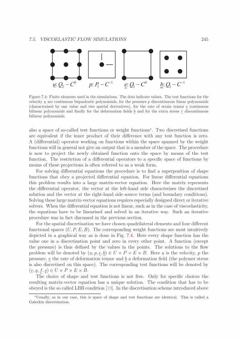
7.5. VISCOELASTIC FLOW SIMULATIONS 245
Figure 7.4: Finite elements used in the simulations. The dots indicate values. The test functions for thevelocity u
¯are continuous biquadratic polynomials, for the pressure p discontinuous linear polynomials
(characterised by one value and two spatial derivatives), for the rate of strain tensor e¯
continuousbilinear polynomials and finally for the deformation fields b
¯and for the extra stress τ
¯discontinuous
bilinear polynomials.
also a space of so-called test functions or weight functions∗. Two discretised functionsare equivalent if the inner product of their difference with any test function is zero.A (differential) operator working on functions within the space spanned by the weightfunctions will in general not give an output that is a member of the space. The procedureis now to project the newly obtained function onto the space by means of the testfunction. The restriction of a differential operators to a specific space of functions bymeans of these projections is often referred to as a weak form.
For solving differential equations the procedure is to find a superposition of shapefunctions that obey a projected differential equation. For linear differential equationsthis problem results into a large matrix-vector equation. Here the matrix representsthe differential operator, the vector at the left-hand side characterises the discretisedsolution and the vector at the right-hand side source terms (and boundary conditions).Solving these large matrix-vector equations requires especially designed direct or iterativesolvers. When the differential equation is not linear, such as in the case of viscoelasticity,the equations have to be linearised and solved in an iterative way. Such an iterativeprocedure was in fact discussed in the previous section.
For the spatial discretisation we have chosen quadrilateral elements and four differentfunctional spaces (U, P,E,B). The corresponding weight functions are most intuitivelydepicted in a graphical way as is done in Fig. 7.4. Here every shape function has thevalue one in a discretisation point and zero in every other point. A function (exceptthe pressure) is thus defined by the values in the points. The solutions to the flowproblem will be denoted by (u
¯, p, e
¯, b¯) ∈ U × P × E × B. Here u
¯is the velocity, p the
pressure, e¯
the rate of deformation tensor and b¯
a deformation field (the polymer stressis also discretised on this space). The corresponding test functions will be denoted by(v¯, q, f
¯, s¯) ∈ U × P × E ×B.
The choice of shape and test functions is not free. Only for specific choices theresulting matrix-vector equation has a unique solution. The condition that has to beobeyed is the so called LBB condition [19]. In the discretisation scheme introduced above
∗Usually, as in our case, this is space of shape and test functions are identical. This is called aGalerkin discretisation.

246 CHAPTER 7. THE DEFORMATION FIELDS METHOD
it might be surprising to see that there is an extra variable that represents the rate ofstrain e
¯. The mixed Stokes problem, with an extra Newtonian stress contribution τ
¯p
defined on space B gives no stable solution. It violates the LBB condition. To stabilisethe computation the extra variable e
¯is introduced. This variable is the strain-rate
tensor computed by spatial differentiation of u¯
(which is defined on U) and projectionon the (lower dimensional) space E. The computation can be stabilised by addingη(∇u
¯+∇u
¯T −2e
¯) to τp, with η = O(ηp) (which is only nonzero because of the difference
in discretisation) [20]. This quantity then diminishes the influence of the extra stresstensor which is defined on the destabilising function space.
Although the introduction of a new functional space for the stress might seem ratherstrange in the case of Stokes flow, it arises naturally in the viscoelastic problem. Becauseviscoelasticity reduces to Stokes flow for slow flows, the discretisation scheme should atleast obey the stability criteria of the discretised Stokes problem. The introduction of anextra space for the strain-rate E in the discretisation scheme, denoted as DEVSS, wasintroduced by Guenette & Fortin [21]. The name DEVSS comes from discrete EVSS(introduced by R.A. Brown from M.I.T.). The acronym EVSS means elastic viscousstress splitting, which refers to a separate treatment solvent and elastic stresses, but isstrictly speaking incorrect since there is no splitting in DEVSS anymore.
Actually determining the most optimal set of test functions is a matter of trial anderror. For our DEVSS/DG discretisation (DG is explained below) Baaijens et al. [22]found the discretisation as depicted in Fig. 7.4 to be satisfactory. Since we use the samecombination of methods we adopted the same discretisation. The set of equations usedto solve the velocity problem with this discretisation is
(f¯, 2e
¯(n+1) − [∇u
¯(n+1) + (∇u
¯(n+1))T ]) = 0 (7.22)
(q, p(n+1) − 1
ε∇ · u
¯(n+1)) = 0 (7.23)
(∇v¯
T , (ηs + ηadd + η)[∇u¯
(n+1) + (∇u¯
(n+1))T ]− p(n+1)δ¯
+ τ¯
(n+1)p (7.24)
(7.25)
− ηe¯(n+1) − ηadd[∇u
¯(n) + (∇u
¯(n))T ]) = 0,
where η is the DEVSS-viscosity. The equations denote inner products with any testfunction in a function space. The first equation Eq. (7.22) is the projection of the rateof deformation tensor onto space E. The result is stored in e
¯(n+1). The second equation
Eq. (7.23) is the approximate determination of the pressure. Instead of a solving thecoupled set (q,∇·u
¯(n+1)) = 0 with Eq. (7.25), the so called penalty method is used. The
variable ε is small such that elements that are compressed are penalised with a largepressure. The pressure counteracts the compression and thus maintains incompressibilityapproximately. This method is much cheaper and the resulting matrices are smaller.The last equation Eq. (7.25) is the solution of the local force balance using the DEVSSdiscretisation and time stepping routine. This specific form is obtained by performingpartial differentiation in Eq. (7.21) once.
A very important topic in the numerical study of viscoelastic flow is the developmentof a good finite element discretisation scheme. The constitutive equation used mostly

7.5. VISCOELASTIC FLOW SIMULATIONS 247
Figure 7.5: The reason for upwind techniques. To compute inflow, Γine , accurately information from
outside an element is needed. For outflow,Γoute , information within an element is sufficient.
in the benchmarking problems is the upper-convected Maxwell fluid. The problem mostcommonly considered for this purpose is that of a sphere moving in a cylinder (see §7.6).Until quite recently (i.e. about a decade ago) even for relatively low Weissenberg num-ber results of different groups did not agree. At this moment convergent results arefound up to We = 2.6. But not for larger values. This lack of convergence is calledthe high Weissenberg problem. Many researchers think this problem is not a fundamen-tal problem of the constitutive equation, but that it is caused by the imperfection ofthe spatial discretisation scheme (see [10] and [23]). At these high deformation ratesthe polymer stress might behave so differently from a Newtonian viscous stress thatstabilising schemes such as DEVSS do not work any longer.
The part that is missing from the set of equations (7.22)-(7.25) is the update stepof the stress tensor. This step was for the most part discussed in the previous section,except for one very important aspect. The information to calculate the stress is containedin (deformation) fields (here symbolised by b
¯). This information has to move with the
fluid particles. This means the fields have to be convected with the flow. The need toconvect information is the major difference between Stokes flow and viscoelastic flow.In Stokes flow the stress is generated locally and instantaneously. In viscoelastic flowa large part of the current stress is generated in the past. This information has to beconvected with the flow.
The convection problem needs special stabilising techniques (not used for ellipticalproblems such as the Stokes problem). These techniques are generally known as (stream-line) upwind. Within a time step, material, that was upstream with respect to a specificboundary, passes the boundary. In a certain sense it is thus natural to weight infor-mation that is upstream more than information that is downstream when determiningfluxes. This non-symmetric weighting constitutes the difference between a central finitedifference scheme and a upwind finite difference scheme.
248 CHAPTER 7. THE DEFORMATION FIELDS METHOD
The discontinuous Galerkin scheme [24] we use in our simulations is similar. In thediscontinuous Galerkin discretisation one allows the discrete solution to make jumpswhen crossing element boundaries. The Finger tensor fields are discretised in this way.This can be inferred from Fig. 7.5 by noting that there are no boundary nodes for theseelements. The effect is a (partial) decoupling of the evolution in nodes of neighbouringboundaries. In the ‘classical’ continuous weak formulation a convection term u
¯· ∇b
¯is
discretised as
(s¯
: u¯· ∇b
¯). (7.26)
The convection term is however a differential representation of the flux across a boundary,and only valid if functions are differentiable. So, for the use in a discontinuous Galerkindiscretisation, the representation is correct within elements, but there is a problem aselement boundary are crossed. If one makes a control volume around a boundary ofan element, one will find a flux is disappearing into this boundary (which has measurezero). This is not into accordance with the underlying physical problem: macroscopicallylarge fluxes are not allowed to disappear into nothing. The solution to this problem isto divide this extra flux between the two neighbouring elements. The choice made forthe discontinuous Galerkin discretisation is upwind-like. The extra boundary-flux fullycontributes to the evolution in the downstream element and nothing to the evolution inthe other neighbouring element. This means the discontinuous Galerkin discretisationof the convection term becomes
(s¯, u¯· ∇b
¯) +
∑e
∫Γin
e
(u¯· n¯)s¯
: (b¯neighb − b
¯)dΓ, (7.27)
where b¯neighb denotes the value at the other side of the boundary in the neighbouring
element. It is important to note that the boundary integrals reestablish a couplingbetween elements. This is however a one-way coupling (information is transported fromone element to its neighbour but not back) and is numerically still very efficient.
The convection of the deformation fields is the last ingredient needed to completea time step in the deformation fields flow solver. In fact, a time step starts out withthe deformation and convection of the deformation fields (via Eq. (7.8) and Eq. (7.27)).Next the polymer stress is determined by Eq. (7.14). The polymer stress can be usedas a source term to solve the Stokes problem Eqs. (7.22)-(7.25). This flow diagram isdepicted in Fig. 7.6.
7.6 Validation of the method: UCM
In this section the deformation fields method will be benchmarked. To this end weselected the well-known geometry of a sphere moving along the centreline of a cylindricaltube filled with a upper-convected Maxwell (UCM) fluid. Because the UCM model alsohas an integral formulation, the deformation fields method can be used. The results willbe compared with those obtained from various differential approaches. The large amount
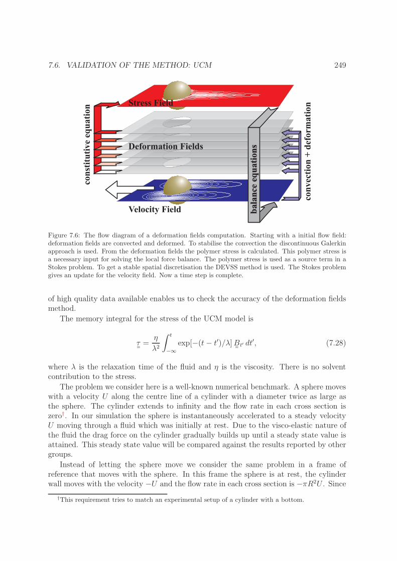
7.6. VALIDATION OF THE METHOD: UCM 249
Figure 7.6: The flow diagram of a deformation fields computation. Starting with a initial flow field:deformation fields are convected and deformed. To stabilise the convection the discontinuous Galerkinapproach is used. From the deformation fields the polymer stress is calculated. This polymer stress isa necessary input for solving the local force balance. The polymer stress is used as a source term in aStokes problem. To get a stable spatial discretisation the DEVSS method is used. The Stokes problemgives an update for the velocity field. Now a time step is complete.
of high quality data available enables us to check the accuracy of the deformation fieldsmethod.
The memory integral for the stress of the UCM model is
τ¯
=η
λ2
∫ t
−∞exp[−(t− t′)/λ]B
¯t′ dt
′, (7.28)
where λ is the relaxation time of the fluid and η is the viscosity. There is no solventcontribution to the stress.
The problem we consider here is a well-known numerical benchmark. A sphere moveswith a velocity U along the centre line of a cylinder with a diameter twice as large asthe sphere. The cylinder extends to infinity and the flow rate in each cross section iszero†. In our simulation the sphere is instantaneously accelerated to a steady velocityU moving through a fluid which was initially at rest. Due to the visco-elastic nature ofthe fluid the drag force on the cylinder gradually builds up until a steady state value isattained. This steady state value will be compared against the results reported by othergroups.
Instead of letting the sphere move we consider the same problem in a frame ofreference that moves with the sphere. In this frame the sphere is at rest, the cylinderwall moves with the velocity −U and the flow rate in each cross section is −πR2U . Since
†This requirement tries to match an experimental setup of a cylinder with a bottom.

250 CHAPTER 7. THE DEFORMATION FIELDS METHOD
Figure 7.7: The primary mesh M1 having 68 elements. The meshes used are uniform refinements ofthis mesh. The coarsest mesh used in the calculations, M2, is 2 times refined in both directions, M3 is3 times refined etc.. The finest mesh used is M5. The domain is 30 sphere radii long. Inlet and outletare connected by means of periodic boundary conditions.
we neglect inertia, the equations in the moving frame are identical to the ‘laboratory’frame of reference.
In the simulations we use a flow domain which is 30 sphere radii long. The ends ofthe tube are connected by periodic boundary conditions. We assume no-slip boundaryconditions on the cylinder wall and prescribe the flow rate in the tube. The basic meshis depicted in Fig. 7.7. In the flow computations we use uniform refinement of this basicmesh M1. The coarsest mesh used in the computations, M2, consists of 272 elementswhereas the finest mesh used, M5, contains 1700 elements.
We will make the problem dimensionless using the sphere radius R to scale thespatial dimensions and the relaxation time λ as the characteristic time scale used. TheWeissenberg number is therefore given by
We =Uλ
R. (7.29)
The drag force is divided by the Stokes drag on a sphere moving with the same velocityin an infinite expanse of fluid. The dimensionless drag force thus becomes
K =F
6πηRU. (7.30)
For the finest mesh (M5, 1700 elements) with the smallest time step (∆t = 5 · 10−4
in dimensionless units), a simulation of 24000 time steps using 100 fields took about 24hours on a single processor of a HP9000-J282 workstation. For this time step we useda discretisation of the memory function using the following refinement (see Fig. 7.3) of5 × ∆t, 5 × 2∆t, 7 × 4∆t, 9 × 8∆t, 10 × 16∆t, 10 × 32∆t, 10 × 64∆t, 10 × 128∆t,10× 256∆t, 10× 512∆t, 14× 1028∆t. Adding everything up this yields a large cut-offtime of 12.27 relaxation times. This is the cutoff time taken in most of the calculations.
We typically need a much smaller time step for the evolution of the fields than forthe calculation of the stress integral. The reason is that in the present code a simplefirst-order Euler-forward scheme is used for the time evolution of the deformation fields.This requires small time steps in order to obtain accurate results. The time step requiredfor stability (CFL condition) is much larger. For the stress integral a second orderscheme is used, and larger time steps are allowed here. The first few intervals of the agediscretisation are used to bridge the time interval needed for updating the deformationfields and that for doing the stress integral. If, for example, we use a twice as largetime step as used above (thus ∆t = 10−3) we join the first two intervals (5 × 5 · 10−4,5× 1 · 10−3) and change that to 10 steps of 1 · 10−3. Now the new discretisation, again

7.6. VALIDATION OF THE METHOD: UCM 251
We = 1:8
We = 1:6
We = 1:2
We = 0:8
We = 0:4
We = 0
t
K
76543210
6
5
4
3
2
1
0
Figure 7.8: The time evolution of the dimensionless drag K for the 1:2 geometry.
using 100 fields, becomes 10×∆t, 7× 2∆t, 9× 4∆t, 10× 8∆t, 10× 16∆t, 10× 32∆t,10× 64∆t, 10× 128∆t, 10× 256∆t, 14× 512∆t. So after the bridging of the differencein time steps the whole discretisation stays the same, except for a small change in thefirst intervals. Having experimented with several other discretisations, both using moreand less fields, we concluded that the error introduced by the discretisation presentedabove using 100 fields is much smaller than the errors caused by the time evolution ofthe deformation fields. Optimisation of the truncation error may lead to a number offields that is smaller than 100, but we have not explored this possibility yet.
The time evolution of the drag for mesh M5 is plotted in Fig. 7.8 for various valuesof We. To obtain the stationary values, the drag was monitored up to 12 times therelaxation time. For such large times the asymptotic values of the drag are very closelyapproached. To determine the asymptotic value we fitted the tail (t > 8λ) to a constantplus a decaying exponential. As will be discussed below, for high Weissenberg numberthe calculation becomes unstable before t = 12λ can be reached. For these Weissenbergnumbers we did the extrapolation for a time interval that started earlier, giving slightlyless accurate results. For higher Weissenberg numbers (we only tried We = 2.0) thecomputations become unstable very quickly and no useful results can be obtained.
In the current implementation, the evolution of the deformation fields is the mostimportant part affecting accuracy and stability. The first graph in Fig. 7.9 shows therelative difference of the computed drag compared with values reported in literature fordifferent meshes at various Weissenberg numbers. The literature values are taken fromWarichet & Legat [25], which are considered to be the most accurate up to now. Thetime step used is 1 · 10−3. The results for the meshes M4 an M5 superimpose, but theerror does not vanish. This is due to the fact that even in the stationary case an errordue to the time discretisation persists. The solution of the evolution equations for the

252 CHAPTER 7. THE DEFORMATION FIELDS METHOD
deformation fields Eq. (7.7) does not become stationary. Even if the velocity field v¯(x¯, t)
is stationary, a Finger tensor field created at some reference time t′ will keep beingdeformed. This gives rise to a permanent time discretisation error in the B
¯t′ ’s and thus
in the stress, which is a weighted sum of these tensors.The second graph of Fig. 7.9 shows the time step convergence of the dimensionless
drag using the most refined mesh M5. Three time steps were studied 5 ·10−3, 1 ·10−3 and5 · 10−4. As can be seen very small time steps have to be used to obtain high accuracyresults. This is basically a result of the first-order time discretisation being used for theevolution equation of the deformation fields. A small time step is inconvenient becausethe number of time steps needed increases and thus also the total CPU time. Thissituation can be improved by using higher-order time integration, but we have not donethat yet.
A more serious problem is the occurrence of instabilities, which are related to theoldest deformation fields becoming too distorted. Because in the evolution of the de-formation fields there is no relaxation mechanism, errors are not damped. When fieldsbecome too distorted, errors grow too rapidly and the field computation may becomeunstable. If the error in the oldest fields become too large it significantly contributes tothe stress and causes the full problem to become unstable.
In Fig. 7.10 we monitored the first occurrence of instability‡ in the drag for thestartup problem we are considering. This time of onset of instability is indicated bytinst. In order to avoid any influence of the cutoff time here, the value of τc is taken tobe considerably larger than tinst. The dependence of tinst on the Weissenberg numberfor mesh M3 is depicted in the first graph of Fig. 7.10. It appears that in the rangeWe = 1.4–1.6 the type of instability changes. For the first ‘branch’ we find that the timeof instability can approximately be described by a linear curve given by
Utinst
R= 11.7 + 4We. (7.31)
In terms of the time scale λ this can also be written as
tinst
λ=
11.7
We+ 4, (7.32)
which shows that tinst becomes smaller with respect to the relaxation time λ for largervalues of We. No instabilities are found below We = 0.8 for mesh M3. This indicates thatfor small Weissenberg numbers the growth rate of the errors in the fields is smaller thanthe rate of decay of the memory function in the stress calculations. The second graphin Fig. 7.10 depicts the mesh dependency of tinst for We = 1 and We = 1.7. For a morerefined mesh the instability occurs later for We = 1, but for We = 1.7 the result is lessregular and for mesh M5 the time of instability decreases compared to mesh M4. Furtherrefinement of the mesh is needed to see whether we find real mesh convergence for thehigher Weissenberg numbers. However, this will require more computer resources and
‡The first occurrence of the instability is defined as the point where there is a significant visible‘jump’ in the drag, which seems to be rather independent from the time discretisation. After this jumpthe flow becomes unstable.

7.6. VALIDATION OF THE METHOD: UCM 253
We = 0:2
We = 0:4
We = 0:6
We = 0:8
We = 1:0
We = 1:2
We = 1:4
We = 1:6
We = 1:8
t
K Klit
Klit
0.0050.0040.0030.0020.0010
0.025
0.02
0.015
0.01
0.005
0
-0.005
M5
M4
M3
M2
We
K Klit
Klit
1.81.61.41.210.80.60.40.20
0.02
0.015
0.01
0.005
0
-0.005
Figure 7.9: Mesh convergence and time convergence for the UCM case of the dimensionless drag forceK relative to the most accurate values reported in the literature [25]. The first graph demonstratesmesh convergence for different uniformly refined meshes. The time step used is 1 · 10−3. The secondgraph shows the linear convergence toward for decreasing time steps. Here mesh M5 is used.

254 CHAPTER 7. THE DEFORMATION FIELDS METHOD
We = 1:7, t = 0:001We = 1, t = 0:001We = 1, t = 0:01
mesh renement factor
Utinst
R
5432
23
22
21
20
19
18
17
16
15
14
13
12
11
10
9
11:7 + 4Wesecond instabilityrst instability
We
Utinst
R
1.81.61.41.210.8
18
17
16
15
14
13
Figure 7.10: The time of the onset of instability tinst in the simulations is monitored as function of Wefor mesh M3 (top figure) and mesh refinement for We = 1 and We = 1.7 (bottom figure).

7.6. VALIDATION OF THE METHOD: UCM 255
Warichet & LegatRasmussen & HassagerPresent results (UCM)
Rouse Chain
We
K
1.81.61.41.210.80.60.40.20
6
5.5
5
4.5
4
Figure 7.11: The dimensionless drag K versus the Weissenberg number We, for the 1:2 geometry.
will be part of future work. The dependence on the time step is also shown in Fig. 7.10for We = 1. As can be seen there is almost no time step dependence.
A simple remedy for the occurrence of instabilities that comes to mind is reducing thecutoff time τc. In this way the ‘life time’ of a field is reduced such that it cannot becomedistorted too much and generate an instability. We have done various computationsthat confirm this statement. Furthermore, it seems that the tinst as shown in Fig. 7.10is a good measure for the maximum cutoff time τc that removes the instability. At first,this is somewhat surprising since tinst is measured in the start-up flow. However, notethat when starting to move the sphere one immediately enforces a Stokesian flow fieldhaving a flow rate that does not change during the computations. Depending on theWeissenberg number the stationary flow field will differ from the initial field, but notsignificantly. Therefore the deformation fields experience an approximately stationaryflow field even in the start-up flow. The practical solution is thus to make the cutofftime small enough. A small cutoff time however introduces an inaccuracy in the stressintegral. We found that imposing a small enough cutoff time does not give significantinaccuracies for We smaller than or equal to 1.4. For higher Weissenberg numbers thetime of instability is smaller, as can be seen in Fig. 7.10. This means that the cutofftimes that have to be taken to avoid the instability dominate the errors in the drag anda comparison with literature values would not be meaningful.
The stationary values of the dimensionless drag K are plotted in Fig. 7.11 and listedin Tab. 7.1 as a function of We. The results are obtained by using the most refined mesh(M5) and by extrapolating the results of the drag for different time steps to ∆t = 0(see Fig. 7.9). Furthermore, we used a cutoff time τc = 12.27λ for all calculations. Thismeans, that for the higher Weissenberg numbers the cutoff time is too small to avoid
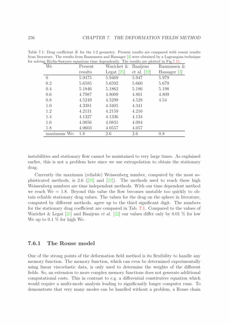
256 CHAPTER 7. THE DEFORMATION FIELDS METHOD
Table 7.1: Drag coefficient K for the 1:2 geometry. Present results are compared with resent resultsfrom literature. The results from Rasmussen and Hassager [3] were obtained by a Lagrangian techniquefor solving Rivlin-Sawyers equations time dependently. The results are plotted in Fig.7.11.
We Present Warichet & Baaijens Rasmussen &results Legat [25] et al. [22] Hassager [3]
0 5.9475 5.9469 5.947 5.9790.2 5.6585 5.6592 5.660 5.6790.4 5.1846 5.1862 5.186 5.1980.6 4.7987 4.8009 4.801 4.8090.8 4.5249 4.5299 4.528 4.541.0 4.3381 4.3405 4.3411.2 4.2131 4.2159 4.2161.4 4.1327 4.1336 4.1341.6 4.0856 4.0831 4.0841.8 4.0603 4.0557 4.057maximum We: 1.8 2.6 2.6 0.8
instabilities and stationary flow cannot be maintained to very large times. As explainedearlier, this is not a problem here since we use extrapolation to obtain the stationarydrag.
Currently the maximum (reliable) Weissenberg number, computed by the most so-phisticated methods, is 2.6 ([25] and [22]). The methods used to reach these highWeissenberg numbers are time independent methods. With our time dependent methodwe reach We = 1.8. Beyond this value the flow becomes unstable too quickly to ob-tain reliable stationary drag values. The values for the drag on the sphere in literature,computed by different methods, agree up to the third significant digit. The numbersfor the stationary drag coefficient are compared in Tab. 7.1. Compared to the values ofWarichet & Legat [25] and Baaijens et al. [22] our values differ only by 0.01 % for lowWe up to 0.1 % for high We.
7.6.1 The Rouse model
One of the strong points of the deformation field method is its flexibility to handle anymemory function. The memory function, which can even be determined experimentallyusing linear viscoelastic data, is only used to determine the weights of the differentfields. So, an extension to more complex memory functions does not generate additionalcomputational costs. This in contrast to e.g. a differential constitutive equation whichwould require a multi-mode analysis leading to significantly longer computer runs. Todemonstrate that very many modes can be handled without a problem, a Rouse chain

7.7. Q-TENSORS 257
of 100 modes is simulated. The memory function in this case becomes:
M(τ) =
100∑k=1
(sin[πk/202]
sin[π/202]
)2
exp
[−(
sin[πk/202]
sin[π/202]
)2τ
λ
]. (7.33)
Results using mesh M4 and ∆t = 5 · 10−4 are plotted in Fig. 7.11. In this calculationthe We number is based upon the largest relaxation time in the spectrum, i.e. λ.
7.7 Q-tensors
The terminology ‘Q-tensor’ is borrowed from reptation theory. This Q-tensor quantifiesthe mean orientation of tube segments. Here we will use it more generally to denote non-linear measures of strain f
¯[B¯] as occurring in the Rivlin-Sawyers equation Eq. (7.9). As
discussed in appendix 6.B page217 of the previous chapter a three dimensional isotropictensor function of a symmetric tensor, f
¯[B¯], can be written as
Q¯
= f¯[B¯] = f1(IB, IIB)B
¯+ f2(IB, IIB)B
¯−1, (7.34)
where IB = tr(B¯) and IIB = tr(B
¯−1) and an isotropic contribution is discarded, because
it contributes to the pressure term. The third invariant IIIB which is the determinant isnot interesting as a variable, because in an incompressible flow it is always 1. Therefore,to be able to simulate any Q-tensor in an arbitrary flow field two scalar functions (f1 andf2) of two scalar variables (IB and IIB) have to be known. The only two tensor quantitiesthat appear are the Finger tensor and its inverse. For example for the independentalignment Doi-Edwards tensor a very good approximation is given by Currie [26]
Q¯
(DE−IA) ≈ 1(IB − 1 + 2
√IIB + 13/4
)[B¯− 1√
IIB + 13/4B¯−1
]. (7.35)
The microscopic expression for Q¯
(DE−IA) is
Q¯
(DE−IA) =
⟨Q¯Q¯|Q
¯|2⟩. (7.36)
Here the vector Q¯
is an initially isotropically distributed vector which is deformed affinelyas follows
Q¯
= F¯·Q¯
0. (7.37)
That theQ-tensor can be written as a function of the Finger tensorB¯
= F¯·F¯
T is a generalconsequence of objectivity and isotropy us discussed previously. In this specific case itcan more easily be inferred from the rotation invariance of the isotropic distribution.

258 CHAPTER 7. THE DEFORMATION FIELDS METHOD
Using this knowledge one is allowed to make the special choice F¯
:= B¯
12 . Inserting this
result into Eq. (7.36) gives
Q¯
(DE−IA) =
⟨B¯
12 ·Q
¯0Q¯
0 · B¯
12
|B¯
12 ·Q
¯0|2
⟩. (7.38)
In some simulation presented in §7.8.2 this microscopic expression is used. The isotrop-ically distributed vectors Q
¯0 are generated stochasticly using a method introduced by
van Heel et al. [5]. In that approach M (typically 20-40) unit vectors Q¯
0 are distributedon the surface of the unit sphere. In order to approximate a uniform distribution onthe surface, the M vectors are not distributed randomly, but we distribute them suchthat they cover the sphere surface as homogeneously as possible. This approach givesthe exact value of Q
¯in the limit of large M , but from our simulations we found that a
number of M = 40 unit vectors, distributed as described above, is sufficient.The calculation of the stress using the isotropically distributed ensemble is rather
expensive compared to the use of the Currie expression (about a factor 5 as expensiveand less precise). The disadvantage of the Currie expression is of course that it is anapproximation (but an accurate one both in shear and elongation). It is however alsopossible to use interpolation functions for f1 and f2 arising in Eq. (7.34). These functionscan be determined with very high accuracy beforehand (see previous chapter appendix6.B page217). For two dimensional flow this procedure becomes extremely simple. Nowthe Cayley-Hamilton theorem states that any isotropic function of a symmetric tensorcan be expressed as a function of the two invariants times the isotropic tensor plus sucha function times the symmetric tensor itself. In the case of incompressible one invariantof the Finger tensor, namely the determinant, is constant. The isotropic contribution isnot interesting because it gives rise to a pressure term. Therefore
Q¯
= f(IB)B¯, (7.39)
with B¯
the two dimensional Finger tensor. The methodology for construction f(IB)is to generate (diagonal) deformation gradient tensors and then calculate both IB andtr(Q
¯)2D (= f(IB)IB) by means of a numerical experiment. These values are stored in
a interpolation function which is used in the deformation fields method via Eq. (7.39).We have implemented this method not only for the independent alignment Doi-Edwardstensor, but also for the rigorous one
Q¯
(DE) =
⟨Q¯Q¯|Q
¯|⟩/〈|Q
¯|〉. (7.40)
Also the f(IB) for the various strain functions, such as those corresponding to ellipticcross sections (see appendix 6.B) can be easily determined and used in flow calculationswithout any extra costs.
Alternatively f() can be obtained from the experimental damping function h(γ). Bydefinition, the shear stress immediately subsequent to a step shear strain of γ is
τxy = G0h(γ)γ. (7.41)
7.7. Q-TENSORS 259
The Finger tensor is
B¯
=
(1 + γ2 γγ 1
)(7.42)
Which gives
τxy = G0h(γ)γ = G0f(2 + γ2)γ, (7.43)
(with G0 =∫∞0M(τ)dτ).
7.7.1 Papanastasiou-Scriven-Macosko
With the introduction of a nonlinear strain measure any hope to reduce a integral equa-tion to a differential equation (without making approximations) is lost. To our knowledgethe only time-dependent implementation of a non-trivial Rivlin-Sawyers model, that ap-peared in the literature so far is by Rasmussen & Hassager [9]. The model they use is thePapanastasiou-Scriven-Macosko (PSM) model, belonging to the class of Rivlin-Sawyersequations. The constitutive equation for the PSM model is given by
τ¯
=ηp
λ2
∫ t
−∞exp[−(t− t′)/λ]
α
α− 3 + βIB + (1− β)IIBB¯
t′ dt′, (7.44)
where ηp is the contribution of the extra stress τ¯
to zero-shear-rate viscosity and IB, andIIB are the first and second invariants of B
¯t′ . This model has the convenient property
that one parameter (β) has no influence on the behaviour of the model in simple shearflow. This parameter can thus be used to fit the elongational behaviour without affectingthe properties in shear flow. For high values of the parameter α the model effectivelybecomes identical to the UCM model.
Rasmussen & Hassager [9] compared their computational results to experimentaldata obtained by Becker et al. [27] on spheres with a radius of 1.27 cm settling ina cylindrical tube with a radius of 5.23 cm. The fluid is characterised in shear flowwhich resulted in the following values of the parameters: ηs = 12.37 Pa s, ηp = 8.60Pa s, λ = 1.21 s and α = 25000. Note that a viscous contribution (solvent) is presentin the model. We have neglected inertia in our calculations. The effect of inertia inthis problem (the elasticity number is equal to 38.1 [27, 9]) is very small. We did somecalculations with inertia included and the drag difference was less than 0.1% for theWeissenberg numbers considered here. The parameter β was varied in the simulationto explore the effect of the elongational properties on the settling velocity. The value ofα is very large so only for large deformations, i.e. large We, deviations from the UCMfluid will occur. The largest deformations in the falling sphere geometry occur near thecentreline, in the wake of the cylinder, where strong elongational flow is present.
The mesh being used is similar to that of mesh M4 in the UCM computation, howeverwith an extra rectangular region between the previous position of the wall (two timesthe sphere radius) and the new position of the wall. The time step used is 1 · 10−3.

260 CHAPTER 7. THE DEFORMATION FIELDS METHOD
= 1 = 0:25Oldroyd-B = 1 = 0:25 = 0Oldroyd-B
Hassager ['96]Rasmussen &
Present Results
We
K
4.543.532.521.510.50
2.4
2.3
2.2
2.1
2
1.9
Figure 7.12: The drag coefficient K as a function of We for the PSM model. Values are compared todata of Rasmussen and Hassager [9].
The stationary results are shown in Fig. 7.12 and are obtained in the same way as forthe UCM model (see section 7.6). The results of Rasmussen and Hassager [9] showthe same trends as our results. For the We → 0 limit we obtain the exact Newtonianresult K = 1.931 [28]. In the regime where the results for different β’s superimpose ourresults superimpose with those of [9] (see Fig. 7.12). For higher values of the We numbermodels with a different value of β start to generate different predictions for the dragforce. In this regime the deformations in the flow are apparently large enough to makea difference between the models with different values of β. It is also clear that there is asmall (less than 1.5%), but significant difference between our results and those obtainedby Rasmussen & Hassager.
7.8 Models with flow dependent life time distribu-
tions
In many models for polymer melts such as the Doi-Edwards model and the Mead-Larson-Doi model the average orientation of segments S
¯is a key quantity. This quantity can
be related to the deformation history via
S¯(x¯, t) =
∫ t
−∞µ(x
¯, t, t′)Q
¯(x¯, t, t′)dt′, (7.45)
see appendix 6.C. Here Q¯(x¯, t, t′) is a tensor characterising the mean orientation at time
t of tube segments that were created at time t′. As discussed §7.7 this tensor can be

7.8. MODELS WITH FLOW DEPENDENT LIFE TIME DISTRIBUTIONS 261
easily§ related to the Finger tensor B¯
t′(x¯, t), Q
¯(x¯, t, t′) = f
¯[B¯
t′(x¯, t)].
The factor µ(x¯, t, t′)dt′ denotes a fraction of all tube segments. This fraction is
the fraction that is created in the time interval [t′, t′ + dt′] and which is still presentat the present time t. To be able to model more advanced constitutive models formelts such as the Mead-Larson-Doi model [8], the pom-pom model [7] and the modeldiscussed in the previous chapter 6, it is necessary to go beyond the limitations of Rivlin-Sawyers equations where µ(x
¯, t, t′) = M(t − t′)/G0 (where G0 is the plateau modulus
G0 =∫∞0M(τ)dτ).
The most general form for the time evolution of µ(x¯, t, t′) in these models, see e.g.
Eq. (6.23), is
D
Dtµ(x
¯, t, t′) = − 1
τ(x¯, t, t′)
µ(x¯, t, t′), (7.46)
where τ(x¯, t, t′) is the relaxation time of a segment at position x
¯with reference time t′.
By definition we have ∫ t
−∞µ(x
¯, t, t′)dt′ = 1. (7.47)
Differentiating this equation once gives
µ(x¯, t, t) = −
∫ t
−∞
D
Dtµ(x
¯, t, t′)dt′ =
∫ t
−∞
1
τ(x¯, t, t′)
µ(x¯, t, t′)dt′, (7.48)
i.e. the initial value of µ(x¯, t, t′) at t′ = t. Which states that the fraction of segments
created per unit time equals the fraction of segments annihilated in the same time span.A constant relaxation time, τ(x
¯, t, t′) = τ , gives a simple exponential decay. A much
less trivial case is that of a relaxation time that depends on position on current time,
τ(x¯, t, t′) = τ(x
¯, t). (7.49)
This is e.g. the case for the Mead-Larson-Doi model. For this case the rate of creationis
µ(x¯, t, t) =
1
τ(x¯, t)
, (7.50)
(found by substitution of Eq. (7.49) into Eq. (7.48)).Equilibrium relaxation mechanisms are incorporated into the memory functionM(t−
t′). For larger deformation, independent relaxation mechanisms induced by the flow,such as convective constraint release, might come into play. When these mechanismsare really independent of the linear response then the total survival probability densityis
µ(x¯, t, t′) =
1
G0
M(t− t′)µFLOW(x¯, t, t′). (7.51)
§at least in two dimensional flow

262 CHAPTER 7. THE DEFORMATION FIELDS METHOD
The survival probability µFLOW(x¯, t, t′) deviates from one only in the non-linear regime.
We will here assume¶
D
DtµFLOW(x
¯, t, t′) = −k(x
¯, t)µFLOW(x
¯, t, t′). (7.52)
The evolution of the total survival probability density is obtained, by differentiatingEq. (7.51) to time and substituting Eq. (7.52), to be
D
Dtµ(x
¯, t, t′) = −
[ −1
M(t− t′)d
dtM(t− t′) + k(x
¯, t)
]µ(x
¯, t, t′). (7.53)
As expected for independent processes the decay rates add up. By substituting the totaldecay rate into Eq. (7.48) one will find that
µFLOW(x¯, t, t) =
1
M(0)
G0k(x
¯, t)−
∫ t
−∞
dM(t− t′)dt
µFLOW(x¯, t, t′)dt′
. (7.54)
In computing the mean orientation tensor, the two relaxation terms are treateddifferently
S¯
=1
G0
∫ t
−∞M(t − t′)µFLOW(x
¯, t, t′)Q
¯(x¯, t, t′)]dt′. (7.55)
The function M() is treated exactly the same as in the Rivlin-Sawyers case, see §7.4.1. Itgives rise to pre-calculated weights. To take account of the non-linear effects contained inµFLOW(x
¯, t, t′) a new series of scalar field indexed by their reference time t′ is introduced.
We will call these fields the weight fields because they constitute an extra weightingfactor in the integral. Similarly to the Finger tensor fields B
¯t′(x
¯, t) they are convected
with the flow and updated according to their evolution equation, Eq. (7.52).Every time step a new weight field is created. Their initial value is given by Eq. (7.54).
This equation is (weakly) implicit. The integral at the right hand side is very simi-lar to the stress integral. As in Eq. (7.15) pre-calculated weights can by used Wi =− ∫∞
0M(τ)φi(τ)dτ to approximate the integral as by a sum. In this discretised form
µFLOW(x¯, t, t) will also appear at the right hand side (with only a small factor in front).
This term can be put to the right hand side. The way the initial condition is incorporatednot by explicitly demanding that the integral Eq. (7.47) is one, but that its derivative totime is zero. This means that, when, due to discretisation errors, it deviates from onethere is no correction. Therefore it may be necessary to renormalise µ(x
¯, t, t′) once in a
while.The Mead-Larson-Doi model has only one relaxation time τd. The linear response is
described by M(t− t′) = G0/τd exp[−(t− t′)/τd]. In this case the evolution of the weightfields is described by
D
DtµFLOW(x
¯, t, t′) = −
[1
τ(x¯, t)− 1
τd
]µFLOW(x
¯, t, t′)
µFLOW(x¯, t, t) =
τdτ(x
¯, t)
.(7.56)
¶The special case we have in mind is the Marrucci convective constraint release mechanism, appendix6.A, where k(x
¯, t) = ∇u
¯(x¯, t) : S
¯(x¯, t).

7.8. MODELS WITH FLOW DEPENDENT LIFE TIME DISTRIBUTIONS 263
7.8.1 Configurational variables
To calculate the stress some configurational variables might be needed. For example forthe Mead-Larson-Doi model one finds
τ¯
p(x¯, t) = 5G0λ
2(x¯, t)S
¯(x¯, t). (7.57)
Here λ(x¯, t) is the so called stretched parameter. (The factor 5 has to do with S
¯being
an orientation tensor). It has its own (fast) dynamics. These kind of configurationalvariables are simple to handle. Precisely as deformation fields and weight fields theyare convected with the flow, and their internal dynamics evolves via a user suppliedequation.
7.8.2 Mead-Larson-Doi
To illustrate the capabilities of the deformation fields method to simulate integral equa-tions other than Rivlin-Sawyers equations this set of simulations uses the Mead-Larson-Doi model [8]. Mead, Larson and Doi have recently developed a reptation model whichcombines two mechanisms that had already been introduced in the literature separately,viz. chain-stretch and convective constraint release (CCR). For a more full discussionsee appendix 6.C.
The reptation model has a flow dependent relaxation time which gives rise to weightfields (see §7.8). Besides orientational contributions to the stress stretch of the polymerinside the tube increases the stress. To simulate the so called stretch parameter an extraconfigurational field is used.
The polymer stress τ¯
p is given by
τ¯
p(x¯, t) = 5G0λ
2(x¯, t)S
¯(x¯, t), (7.58)
where λ is the chain stretch (thus no relaxation time) and S¯
is the orientation tensor.This orientation tensor is calculated using the independent alignment tensor for themean orientation of segments created at t′, see §7.7
S¯(x¯, t) =
∫ t
−∞
1
τdexp[−(t− t′)/τd]µFLOW(x
¯, t, t′)Q
¯
(DE−IA)(x¯, t, t′) dt′, (7.59)
where τd is the reptation time. The partial orientation tensors are both computed usingthe Currie approximation Eq. (7.35) and by the stochastic averaging approach Eq. (7.38).
The creation of segments is flow dependent and dependent on the chain stretch
D
DtµFLOW(x
¯, t, t′) = −
[1
τd
(1
λ2(x¯, t, t′)
− 1
)+k(x
¯, t, t′)
λ(x¯, t, t′)
]µFLOW(x
¯, t, t′), (7.60)
As discussed in §7.8 we have split of the linear viscoelastic memory function. This partis used to compute the constant weights the remaining part, µFLOW(t, t′), constitutes the

264 CHAPTER 7. THE DEFORMATION FIELDS METHOD
0
0.2
0.4
0.6
0.8
1
1.2
1.4
1.6
1.8
0.01 0.1 1 10 100 1000 10000
dim
ensi
onle
ss p
olym
er s
tres
s, τ
p xy/G
0
dimensionless shear rate, γ τd
0.75
0.76
0.77
5 10 15 20 25 30
Figure 7.13: Stress-shear-rate curves for the Doi-Edwards model (solid line) and the Mead-Larson-Doimodel (dotted line), both without added solvent viscosity. The ratio of the reptation time and theRouse time τd/τs = 50. The inset-figure shows the local maximum in the Mead-Larson-Doi model.
weight fields. The factor k is the annihilation rate associated with convective constraintrelease, see appendix 6.C
k = ∇u¯
: S¯− λ/λ. (7.61)
Finally the stretch parameter has its own evolution equation, giving rise to the rapidrelaxation associated with stretch
D
Dtλ = λ∇u
¯: S¯− 1
τs
2
λ+ 1(λ− 1) (7.62)
The first term on the right hand side of Eq. (7.62) corresponds to affine deformation.The second term corresponds to retraction of the polymer by a (linear) spring force.When the stretch is increased the equilibration rate of the contour length is enhanceddue to the convective constraint release. The time-scale associated with this relaxationis the largest Rouse relaxation time of the polymer, τs. In our calculations, followingthe paper of Mead et al. (1998), we fix the ratio of the reptation time τd and the Rousetime τs to 50:
τd/τs = 50. (7.63)
The Doi-Edwards model is recaptured from the Mead-Larson-Doi model by takingλ = 1 and k = 0. In order to compare the Doi-Edwards model and the Mead-Larson-Doi model, we consider their behaviour in stationary shear flow. The curves shown in

7.8. MODELS WITH FLOW DEPENDENT LIFE TIME DISTRIBUTIONS 265
Fig. 7.13 were obtained using the deformation-field implementation (which is describedin the following sections), and they are found to reproduce the results of Mead, Larsonand Doi [8], who calculated the curves in a different way. Note that the Doi-Edwardsmodel has a shear-stress maximum, followed by excessive shear thinning. As was alreadymentioned above, this shear thinning is a consequence of the alignment of the polymersin the direction of the flow. The Mead-Larson-Doi reptation model leads to a completelydifferent curve. Roughly speaking, there are three shear-rate regimes: for shear ratesγ < 1/τd, the Mead-Larson-Doi model is qualitatively the same as the Doi-Edwardsmodel. For shear rates in the range 1/τd < γ < 1/τs, CCR will be dominant andthe shear stress will remain more or less constant as a function of shear rate. FromFig. 7.13 we can see that the stress has a local maximum (τxy = 0.764G0) at a shearrate of γ = 6.2/τd. After this local maximum the stress remains nearly constant butdecreases until a shear rate of γ = 18.5/τd, at which point the shear stress has a localminimum (τxy = 0.755G0). Finally, for shear rates γ > 1/τs, the flow is strong enoughto stretch the polymers, leading to an increase in stress again. At very high shear rates,γ ≈ 20/τs (or 1000/τd), the stress decreases again and suffers extreme shear thinning.In this range, however, also higher Rouse relaxation modes, which are omitted in theMead-Larson-Doi model, should be taken into account. Therefore, at these very highshear rates the model is no longer applicable.
To illustrate the use of the Mead-Larson-Doi model in a complex flow simulation,we use the ‘cylinder in a channel’ geometry. This is a two-dimensional geometry. Thewidth of the channel is twice the diameter of the cylinder and the cylinder is placedon the centreline. Periodic boundary conditions are used to connect the inlet and theoutlet of the channel for all quantities except the pressure, which is periodic up to alinear function. By taking the total length of the channel to be thirty times the cylinderradius, the interaction of the cylinder with its mirror images is negligible.
Fig. 7.14 shows the mesh that we use in the calculations (referred to as M2). At thecylinder wall the width of an element is 0.025R, where R is the cylinder radius. At thechannel wall, the width is 0.033R. Mesh M2 consists of 2048 elements. For the purposeof investigating mesh convergence we use a coarser mesh (M1 , coarsened by a factor0.75 in all directions), and a finer mesh (M3, refined by a factor 1.25).
For all simulations presented in this section a time step of ∆t = 0.001 τd is used.This is sufficient to simulate the reptation process accurately. The stretch time is afactor 50 smaller than the reptation time. This means it is 20 times larger than thediscretisation time step. In simulations of transient flows, using the Mead-Larson-Doimodel, this will give rise to a small discretisation error. In steady flow this error isabsent. The reason is that, in our implementation, the numerical method to solve thediscretised stretch equation becomes independent of the time step for flows which arestationary in A Eulerian sense.
Since the effective relaxation time in the Mead-Larson-Doi model depends on the flowfield we have to ensure that the numerical time step in the simulations is sufficiently smalleverywhere in the flow domain. For the Mead-Larson-Doi model this relaxation timehas a minimal value of 0.058 τd in stationary shear flow (at γ = 750 τ−1
d ). The highest

266 CHAPTER 7. THE DEFORMATION FIELDS METHOD
Figure 7.14: Part of mesh M2. The total length of the periodic channel is thirty times the cylinderradius. Differently from the sphere-in-a-tube geometry Fig.7.7 boundary layers wall are expected tooccur at the channel wall. Therefore the mesh is also refined near this wall.
shear rate in our simulations is 50 τ−1d . For this stationary shear rate the relaxation time
is 0.16 τd. In transient situations the relaxation time can be smaller because segmentsare less well aligned (causing the term γ
¯: S
¯to be larger). For γ = 50 τ−1
d the shortestpossible relaxation time is 0.09 τd. The time step used in our simulations, ∆t = 0.001τd,is small enough to resolve all these time scales.
To characterise the flow we use the Weissenberg number based on the cylinder radiusR, and the reptation time τd
We =UτdR
, (7.64)
where U is the mean velocity in the channel.Two sets of flow simulations are presented in this section. The first for We = 0.3 and
the second for We = 0.6. For We = 0.3 we show the results of both the Doi-Edwards fluidand the Mead-Larson-Doi fluid. Secondly we compare a fully deterministic simulationusing the Currie approximation, with a sub-ensemble deformation field simulation, suchas introduced in van Heel et al. [5]. For We = 0.6 some numerical issues like meshconvergence are also discussed.
Flow at We = 0.3
Because of the excessive shear thinning behaviour of the Doi-Edwards model, simulationsbeyond a certain Weissenberg number are unstable. The Mead-Larson-Doi model showsa shallow local stress maximum in the stationary stress-versus-shear-rate relation (seeFig. 7.15). Such a local maximum may lead to instabilities connected to multi-valuednessof the solution (for examples of typical problems related to such a local maximum (see[29], [30] and [31]). Only at extremely high shear rates, which are irrelevant for oursimulations, does the model have a global maximum. Compared to the Doi-Edwardsmodel the Mead-Larson-Doi model is less shear thinning. Nonetheless its behaviour canstill be characterised as very shear thinning. Even at We = 0.3, for the cylinder-in-a-channel geometry, this shear thinning gives rise to extremely thin boundary layers.

7.8. MODELS WITH FLOW DEPENDENT LIFE TIME DISTRIBUTIONS 267
0
0.1
0.2
0.3
0.4
0.5
0.6
0.7
0.8
0 5 10 15 20
dim
ensi
onle
ss p
olym
er s
tres
s, τ
p xy/G
0
dimensionless shear rate, γ τd
Doi-Edwards, CurrieDoi-Edwards, sub-ensembleMLD, CurrieMLD, sub-ensemble
0
0.2
0.4
0.6
0.8
1
1.2
1.4
1.6
1.8
0 5 10 15 20di
men
sion
less
pol
ymer
str
ess,
τp xy
/G0
dimensionless shear rate, γ τd
Doi-Edwards, CurrieDoi-Edwards, sub-ensembleMLD, CurrieMLD, sub-ensemble
Figure 7.15: The stress versus shear rate relations. The left graph shows the relation without extraNewtonian solvent viscosity. The right graph shows the changed relation when 0.05 G0τd is added.Both the Doi-Edwards model and the Mead-Larson-Doi model have lost their excessive shear thinningbehaviour. The values obtained using the Currie approximation are only slightly higher than the exactvalues obtained by using the sub-ensemble expression for the independent-alignment Q
¯-tensor (with
sub-ensemble size M = 20).
These are thinnest on the cylinder wall in the down-stream region. Using the meshesdescribed above, the boundary layers can not be fully resolved. Still finer meshes requiremore computer power (especially more memory) than is available to us.
The Weissenberg number of 0.3 is already quite low and decreasing it even furtheressentially masks the differences between the Doi-Edwards model and the model ofMead, Larson and Doi. Another way to avoid extremely sharp boundary layers is tomake the stress a monotonically increasing function of shear rate by the addition ofextra Newtonian (solvent) viscosity. For the Mead-Larson-Doi model the addition ofan extra solvent viscosity of 0.0015G0τd would have been sufficient to make the steadystate stress monotonically increasing, whereas for the Doi-Edwards model we need toadd a solvent viscosity of 0.03G0τd to achieve monotonicity. For these values of theadded viscosity we still had convergence problems so we were forced to add significantlymore. In the simulations we present here we added a viscosity of ηs = 0.05G0τd to boththe Mead-Larson-Doi and the Doi-Edwards model (see Fig. 7.15). This increases thezero-shear-rate viscosity by 5 %.
Fig. 7.16 shows the drag force after startup of flow at a constant flow rate. The dragforce is made dimensionless by means of elastic scaling, using as unit G0RL, instead ofthe more common viscous scaling (G0τd U L). Here L is the length of the cylinder, whichis irrelevant because the problem is 2D. The left graph shows the response of the Doi-Edwards model. The upper curve is the result of the Currie approximation. The lowercurve shows the sub-ensemble deformation field result. The qualitative behaviour is thesame. There is a small difference in the numerical values at steady state because of thesmall deviation of the Currie approximation from the exact (i.e. for infinite ensemble
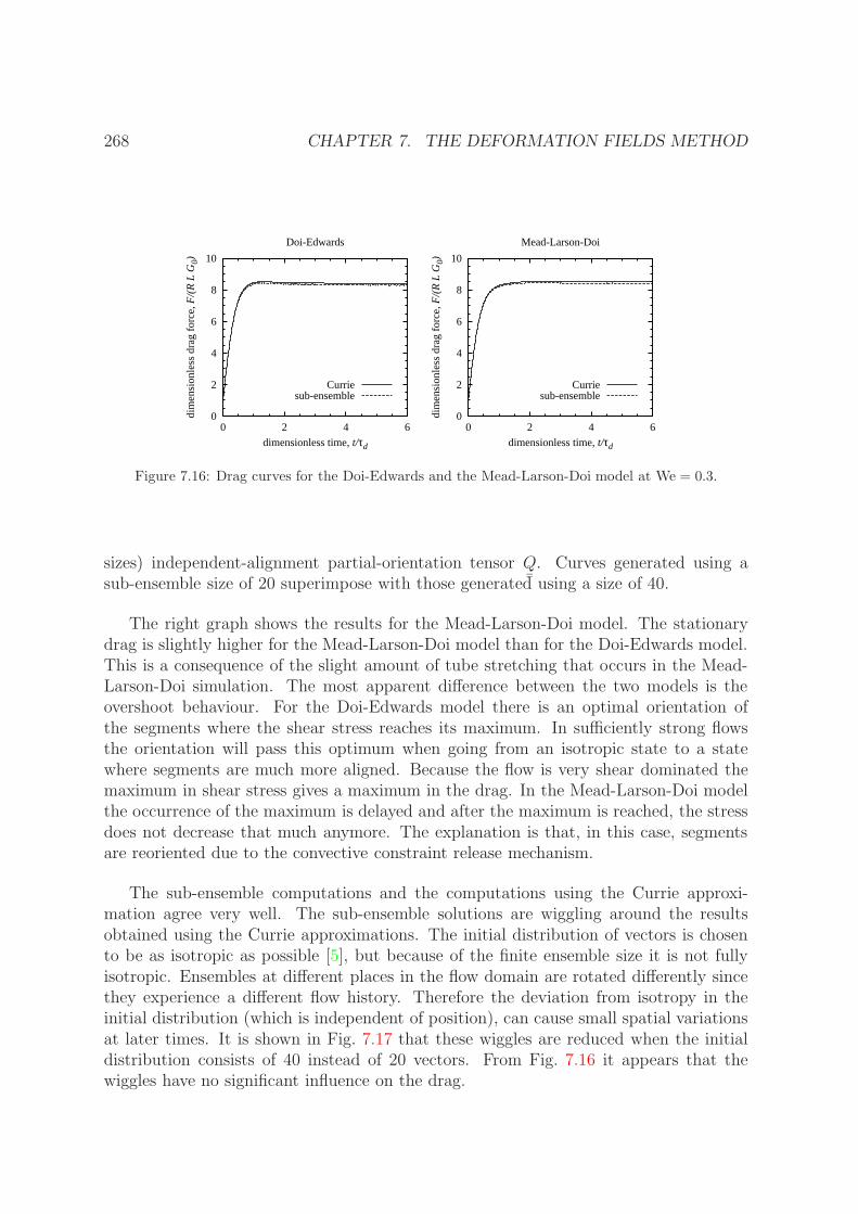
268 CHAPTER 7. THE DEFORMATION FIELDS METHOD
0
2
4
6
8
10
0 2 4 6
dim
ensi
onle
ss d
rag
forc
e, F
/(R
L G
0)
dimensionless time, t/τd
Doi-Edwards
Curriesub-ensemble
0
2
4
6
8
10
0 2 4 6di
men
sion
less
dra
g fo
rce,
F/(
R L
G0)
dimensionless time, t/τd
Mead-Larson-Doi
Curriesub-ensemble
Figure 7.16: Drag curves for the Doi-Edwards and the Mead-Larson-Doi model at We = 0.3.
sizes) independent-alignment partial-orientation tensor Q¯. Curves generated using a
sub-ensemble size of 20 superimpose with those generated using a size of 40.
The right graph shows the results for the Mead-Larson-Doi model. The stationarydrag is slightly higher for the Mead-Larson-Doi model than for the Doi-Edwards model.This is a consequence of the slight amount of tube stretching that occurs in the Mead-Larson-Doi simulation. The most apparent difference between the two models is theovershoot behaviour. For the Doi-Edwards model there is an optimal orientation ofthe segments where the shear stress reaches its maximum. In sufficiently strong flowsthe orientation will pass this optimum when going from an isotropic state to a statewhere segments are much more aligned. Because the flow is very shear dominated themaximum in shear stress gives a maximum in the drag. In the Mead-Larson-Doi modelthe occurrence of the maximum is delayed and after the maximum is reached, the stressdoes not decrease that much anymore. The explanation is that, in this case, segmentsare reoriented due to the convective constraint release mechanism.
The sub-ensemble computations and the computations using the Currie approxi-mation agree very well. The sub-ensemble solutions are wiggling around the resultsobtained using the Currie approximations. The initial distribution of vectors is chosento be as isotropic as possible [5], but because of the finite ensemble size it is not fullyisotropic. Ensembles at different places in the flow domain are rotated differently sincethey experience a different flow history. Therefore the deviation from isotropy in theinitial distribution (which is independent of position), can cause small spatial variationsat later times. It is shown in Fig. 7.17 that these wiggles are reduced when the initialdistribution consists of 40 instead of 20 vectors. From Fig. 7.16 it appears that thewiggles have no significant influence on the drag.

7.8. MODELS WITH FLOW DEPENDENT LIFE TIME DISTRIBUTIONS 269
0
2
4
6
8
10
12
14
-1 -0.5 0 0.5 1
dim
ensi
onle
ss s
hear
rat
e, γ
τ d
dimensionless x-coordinate, x/R
Curriesub-ensemble 20 vectorssub-ensemble 40 vectors
Figure 7.17: Shear rate on the cylinder wall at We = 0.3 for both the Doi-Edwards model (upper curves)and the Mead-Larson-Doi model (lower curves). The sub-ensembles consisting of 20 vectors show smallwiggles. These wiggles are suppressed in simulations using ensembles of 40 vectors. There is almost nodeviation between the Currie approximation and the sub-ensemble calculation.
0
2
4
6
8
10
12
0 1 2 3 4 5 6
dim
ensi
onle
ss d
rag
forc
e, F
/(R
L G
0)
dimensionless time, t/τd
Mead-Larson-DoiDoi-Edwards
Figure 7.18: Drag curves for the Doi-Edwards and the Mead-Larson-Doi model at We = 0.6 using theCurrie potential.
270 CHAPTER 7. THE DEFORMATION FIELDS METHOD
Flow at We = 0.6
At We = 0.6 the qualitative differences between the Doi-Edwards model and the Mead-Larson-Doi model are increased compared to the We = 0.3 situation. Fig. 7.18 showsdrag curves of two calculations using We = 0.6. Although the flow rate has increasedby a factor two, the drag has not increased that much. Most of the increase of the dragis actually due to the viscous solvent contribution and not to the polymer contribution.For the Doi-Edwards model the difference between the value at the ‘overshoot’ peak andthe steady-state value has increased. Furthermore, the overshoot peak is reached earlier.The position of the peak scales with strain. This is fully consistent with the fact thatthe maximum in the drag force is related to an optimum in the segment orientation.
In order to show mesh convergence we investigate the behaviour of the shear rate onthe surface of the cylinder. Results for the different meshes M1, M2 and M3 are plottedin Fig. 7.19. The upper graph shows the situation with an added solvent viscosity of0.05G0τd. The results for the different meshes superimpose under mesh refinement. Thisis completely different for the second graph in Fig. 7.19. Here the solvent viscosity isreduced by a factor of 10 to ηs = 0.005G0τd, which is in fact still sufficient to removethe stress maximum. The shear rates are now much higher and no mesh convergenceis obtained. As discussed in the beginning of this section it is this failure to attainconverged solutions which forced us to add a relatively high amount of solvent viscosity.
The steepness of the boundary layer at the cylinder wall, which is quite large evenfor the added ηs = 0.05G0τd, is illustrated in Fig. 7.20. This plot shows the vorticitycontour of the stationary flow for the We = 0.6 case. On a no-slip wall vorticity isequivalent to the shear rate. The contour lines shown in the figure are separated byan amount of approximately 1.5τ−1
d . Not only large velocity gradients, but also largechanges in velocity gradient are present near the cylinder wall. This steepness increasesdramatically when less solvent viscosity is added.
Fig. 7.21 compares the stretch parameter for We = 0.3 and We = 0.6 on the cylinderwall, again using ηs = 0.05G0τd. Even for the We = 0.6 case the stretch is relativelysmall, only about 5%. At high shear rates the CCR mechanism gives rise to a stationarydistribution of the orientation of tube segments. Deformation and reorientation due toCCR are in equilibrium. This means that, without stretch, the stress will saturate at afinite, maximum value. In the Mead-Larson-Doi model, stretch can provide extra stress.In our simulations, unfortunately this contribution is relatively small compared to thecontribution of the extra solvent contribution. The total polymer stress is 0.8G0 (seeFig. 7.15 at γτd = 16). This is equal to the contribution of the solvent (0.05G0τd×16τ−1
d ).
7.9 Conclusions and discussion
The first and most important conclusion is that the deformation fields method is anew and very useful method to incorporate a large class of constitutive equations intomacroscopic flow simulations.
It was illustrated that the method is capable of simulating time-separable Rivlin-
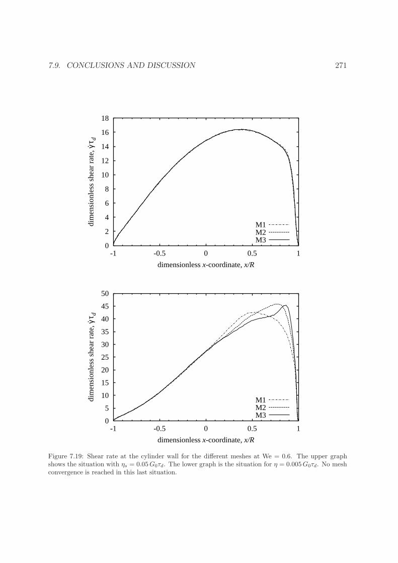
7.9. CONCLUSIONS AND DISCUSSION 271
0
2
4
6
8
10
12
14
16
18
-1 -0.5 0 0.5 1
dim
ensi
onle
ss s
hear
rat
e, γ
τ d
dimensionless x-coordinate, x/R
M1M2M3
0
5
10
15
20
25
30
35
40
45
50
-1 -0.5 0 0.5 1
dim
ensi
onle
ss s
hear
rat
e, γ
τ d
dimensionless x-coordinate, x/R
M1M2M3
Figure 7.19: Shear rate at the cylinder wall for the different meshes at We = 0.6. The upper graphshows the situation with ηs = 0.05 G0τd. The lower graph is the situation for η = 0.005 G0τd. No meshconvergence is reached in this last situation.
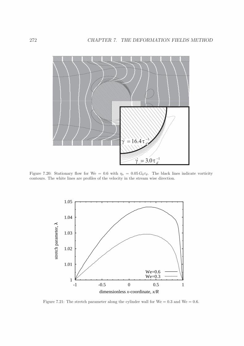
272 CHAPTER 7. THE DEFORMATION FIELDS METHOD
Figure 7.20: Stationary flow for We = 0.6 with ηs = 0.05 G0τd. The black lines indicate vorticitycontours. The white lines are profiles of the velocity in the stream wise direction.
1
1.01
1.02
1.03
1.04
1.05
-1 -0.5 0 0.5 1
stre
tch
para
met
er, λ
dimensionless x-coordinate, x/R
We=0.6We=0.3
Figure 7.21: The stretch parameter along the cylinder wall for We = 0.3 and We = 0.6.

7.9. CONCLUSIONS AND DISCUSSION 273
Sawyers equations in a time-dependent Eulerian setting. The possibility to use arbitraryspectra has been demonstrated by simulations of a Rouse model with 100 modes. Thepossibility to incorporate nonlinear effects has been illustrated using a PSM model.In literature two different approaches to solve Rivlin-Sawyers constitutive equations areknown. The first is a Eulerian method based on streamline integration and is restricted tosteady flows. The second method is a Lagrangian method, where the mesh deforms withthe flow and therefore requires frequent re-meshing to avoid highly distorted elements.The deformation field method combines the advantage of a Eulerian method (no re-meshing, no particle tracking) with the distinct feature of the Lagrangian method (time-dependence).
Since the deformation fields store the full history of deformation the constitutivemodels that can be handled are not restricted to Rivlin-Sawyers equations. In fact, anymodel that obeys the usual assumptions of simple fluid theory (locality, fading memory)can, in principle, be implemented using deformation fields. This opens up the possibilityto explore all kind of new models.
A modest start with this exploration is the implementation of the Mead-Larson-Doi model. In this model the stress consists of two contributions, the stretch andthe mean orientation of tube segments. The orientation is related to the deformationfields by means of an integral relation. To evaluate this integral extra fields have tobe introduced, namely weight fields. These weight fields are used to incorporate extra(nonlinear) relaxation effects, such as convective constraint release.
The stretch parameter is an extra configurational variable. The evolution equationfor such a variable can be included by introducing extra configuration fields. The com-bination of deformation fields, weight fields and configuration fields in one simulationmakes it possible to simulate a large class of melt constitutive equations (e.g. the pom-pom model [7]).
The simulation results presented in this chapter demonstrate that the method isrelatively efficient, since it only uses 100 tensor fields. This is small compared to e.g.stochastic configuration field methods that use 1000 vector fields as a minimum [15].However, it is less efficient than differential models if only a small number of relaxationtimes are used. The better performance of a full deformation fields implementationcompared to a partially stochastic implementation was demonstrated by simulating theMead-Larson-Doi model by the two approaches. The fully ‘macroscopic’ approach usingthe Currie approximation for the orientation Q
¯-tensor and a sub-ensemble approach,
introduced in Van Heel et al. [5], to calculate this Q¯-tensor by ensemble averaging. The
deviation between the Currie approximation and the ‘exact’ sub-ensemble results is verysmall but the CPU time needed was much less (about a factor 5).
The accuracy of the method was investigated by comparing our simulation of themoving sphere UCM benchmark with the most accurate values available from litera-ture. We have shown that our method converges to the literature values when refiningthe spatial and the time discretisation. The integral over the deformation history isapproximated by a finite sum over all fields, which is second-order in time. The defor-mation fields are convected and deformed by the flow. The evolution equation of the

274 CHAPTER 7. THE DEFORMATION FIELDS METHOD
Figure 7.22: Finite element discretisation of the age. The age of the Finger tensors denoted by τ isused as extra variable. Because fields age with a steady rate they move down with a constant velocity.This gives an extra convection term that has to be solved numerically.
fields is solved by a standard finite element technique (discontinuous Galerkin) and afirst-order explicit scheme in time. The latter scheme is the limiting factor for the timestep size. Since even for stationary situations an error due to the time discretisationpersists, very small time steps are needed. Using a higher-order scheme would be amajor improvement.
Even in stationary flow the deformation fields remain unsteady and old fields canbecome too distorted and generate instabilities. These instabilities can be avoided bylimiting the cutoff time in such a way that old fields are removed before becomingtoo distorted. The additional error is dependent on the mesh and the Weissenbergnumber but is usually small. However for high Weissenberg numbers accuracy may beaffected and it is important to check the magnitude of the error. It appears that adifferent instability sets in earlier. The maximum Weissenberg for the cylinder in thetube benchmark of the UCM fluid was We = 1.8. Using the Mead-Larson-Doi modelwe performed complex flow simulations of the ‘cylinder in a channel’ problem at twoWeissenberg numbers (We = 0.3 and We = 0.6). Only after introducing an additionalsolvent viscosity (0.05G0τd) mesh convergence was observed. Unfortunately this highsolvent viscosity somewhat masks the differences between the Doi-Edwards model andthe Mead-Larson-Doi model, which occur mostly at high shear rates.
7.9.1 Future work
Apart from the obvious extensions to new models and refinement of the numerical tech-niques, we believe that a different implementation of the deformation fields idea mightlead to a more simple and efficient scheme. This new way of implementing deformationfields will be discussed in this section.
A major drawback of the implementation discussed in the previous sections is thedifficult bookkeeping. Therefore we will introduce a finite element discretisation of thepast. It is much more flexible than the discretisation discussed in section §7.4.2 andavoids the bookkeeping altogether. In this finite element implementation the age of afield τ is introduced as a new independent variable. This parameterisation of the Finger

7.9. CONCLUSIONS AND DISCUSSION 275
tensor field is easily related to the previous one where the reference time was a primaryvariable
B¯(x¯, t, τ) = B
¯t′(x
¯, t), with t′ = t− τ. (7.65)
The evolution equation of the deformation fields Eq. (7.7) is now transformed by sub-stituting
∂
∂tB¯
t′(x¯, t) =
∂
∂tB¯(x¯, t, t− t′)|t′=const = [
∂
∂tB¯(x¯, t, τ) +
∂
∂τB¯(x¯, t, τ)]τ=t−t′ (7.66)
which gives
∂
∂tB¯(x¯, t, τ) +
∂
∂τB¯(x¯, t, τ) + u
¯(x¯, t) · ∇B
¯(x¯, t, τ)
= (∇u¯)T (x
¯, t) · B
¯(x¯, t, τ) +B
¯(x¯, t, τ) · ∇u
¯(x¯, t). (7.67)
Here it should be realised that in taking the partial derivative to the time variable tthe age τ is kept fixed and not the reference time. The variable τ constitutes an extradimension and gives rise to a extra convection term in the equation. This convectiveterm can be easily interpreted as aging. The age increase with a steady rate. Newlyborn fields have the unit tensor as initial condition B
¯(x¯, t, 0) = δ
¯.
Fig. 7.22 illustrate a two dimensional spatial mesh extended with an extra τ -dimension.This finite element discretisation has obvious advantages. The first is the possibility ofmesh refinement. This is important because at places where deformation rates are largea finer discretisation in the τ direction is probably very useful. One can even think ofadaptive mesh refinement in the τ -direction. This might be a useful tool for simulatingmodels with flow dependent relaxation times as discussed in §7.8. A second advantage isthat the computation of the stress integral is more easy (if a non-adaptive discretisationis used)
τ¯
p(x¯, t) =
∫ ∞
0
M(τ)f¯[B¯(x¯, t, τ)]dτ. (7.68)
Here no complicated bookkeeping is needed. Possibly it can also be made cheaper thanthe method that is currently implemented, by using less discretisation points in theτ -direction. One can increase the size of the elements in the τ -direction more quickly.For streamline integration it is known that evaluation in 10 Laguerre points gives goodresults. A third advantage is that the method is easy to implement for two dimensionalflow if one already has a three dimensional finite element code.
A disadvantage is that an extra discretisation is introduced. In the original imple-mentation fields are labelled by their reference time. Fields with different labels evolveindependently. In the finite element discretisation a convection equation has to be solvedin the τ -direction. This is of course prone to discretisation errors (such as numericaldiffusion). But since this equation is so simple (namely one dimensional and constantvelocity) it can be optimised. At least an upwind scheme should be used, possiblycombined by a discontinuous Galerkin discretisation in the τ -direction.

276 CHAPTER 7. THE DEFORMATION FIELDS METHOD
Another possibility besides the used deformation fields discretisation and the finiteelement discretisation of the τ -direction is a spectral discretisation of this direction. Anobvious choice would be the use of Laguerre polynomials. Both solving the convectionequation and evaluating the integral becomes very simple. It is however less flexiblethan a finite element discretisation.

7.A. REDUCTION OF THE NUMBER OF FINGER TENSOR COMPONENTS 277
7.A Reduction of the number of Finger tensor com-
ponents
Convecting and deforming deformation fields is relatively expensive. Therefore anyreduction in the number of components that need to be computed reduces the storageand CPU requirement proportionally. In an incompressible flow the determinant of theFinger tensor is equal to 1. This means that the tensor components are dependent.Using this dependency the number of tensor components can be reduced by one andthus eliminating the need to store this component in a field.
The Finger tensor has also the property that it is positive definite. The continuousevolution equations make sure that this positive definiteness is maintained. This is notnecessarily the case for the discretised evolution equations. Numerical errors can causethe positive definiteness to be violated. We devised a transformation that simultaneouslyexplicitly imposes the det(B
¯) = 1 and the positive definiteness. We will illustrate this
procedure for the axisymmetric case. The planar case is more simple (take Bθθ = 1,r →∞).
In cylindrical coordinates the Finger tensor is given by Brr 0 Brz
0 Bθθ 0Brz 0 Bzz
, with (BrrBzz − B2
rz)Bθθ = 1. (7.69)
The requirement of positive definiteness in this case gives rise to 4 constraints on thecomponents
Brr > 0, (7.70)
Bzz > 0,
BrrBzz − B2rz > 0,
Bθθ > 0.
The following linear transformation will be applied
µ =√Bθθ
Brr +Bzz
2, (7.71)
ν =√Bθθ
Brr − Bzz
2,
ξ =√BθθBrz.
The constraint det(B¯) = 1 gives
µ =√
1 + ν2 + ξ2. (7.72)
The positive root has to be applied because of positive definiteness, which gives µ > 0.

278 CHAPTER 7. THE DEFORMATION FIELDS METHOD
If one numerically can make sure that√Bθθ is positive the positive definiteness of the
whole tensor is guaranteed. This becomes clear by performing the inverse transformation
Brr = (µ+ ν)/√Bθθ = (
√1 + ν2 + ξ2 + ν)/
√Bθθ, (7.73)
Bzz = (µ− ν)/√Bθθ = (
√1 + ν2 + ξ2 − ν)/
√Bθθ,
BrrBzz − B2rz = 1/Bθθ.
The evolution equation for ν, ξ, µ and√Bθθ are:
Dν
Dt= [
∂vr
∂r− ∂vz
∂z]µ+ [
∂vr
∂z− ∂vz
∂r]ξ, (7.74)
Dξ
Dt= [
∂vr
∂z+∂vz
∂r]µ+ [
∂vz
∂r− ∂vr
∂z]ν,
µ =√
1 + ν2 + ξ2,
D
Dt
√Bθθ
r= 0.
Notice that ν and ξ evolve completely independent of Bθθ.

Bibliography
[1] E.A.J.F. Peters, M.A. Hulsen and B.H.A.A. van den Brule. Instationary Eule-rian viscoelastic flow simulations using time separable Rivlin-Sawyers constitutiveequations. J. Non-Newtonian Fluid Mech., 89(1-2):209–228, 2000.
[2] E.A.J.F. Peters, A.P.G. van Heel, M.A. Husen and B.H.A.A. van den Brule. Gen-eralisation of the deformation field method to simulate advanced reptation modelsin complex flow. J. Rheology, 44(4):811–829, 2000.
[3] H.K. Rasmussen and O. Hassager. Simulation of transient viscoelastic flow. J.Non-Newtonian Fluid Mech., 46:289–305, 1993.
[4] H.K. Rasmussen and O. Hassager. Simulation of transient viscoelastic flow withsecond order time integration. J. Non-Newtonian Fluid Mech., 56:65–84, 1995.
[5] A.P.G. van Heel, M.A. Hulsen and B.H.A.A. van den Brule. Simulation of theDoi-Edwards model in complex flow. J. Rheology, 43(5):1239–1260, 1999.
[6] G. Bishko, T.C.B. McLeish, O.G. Harlen and R.G. Larson. Theoretical molecularrheology of branched polymers in simple and complex flows: The pom-pom model.Phys. Rev. Lett., 79(12):2352–2355, 1997.
[7] T.C.B. McLeish and R.G. Larson. Molecular constitutive equations for a class ofbranched polymers: The pom-pom polymer. J. Rheology, 42(1):81–110, 1998.
[8] D.W. Mead, R.G. Larson and M. Doi. A molecular theory for fast flows of entangledpolymers. Macromolecules, 31(22):7895–7995, 1998.
[9] H.K. Rasmussen and O. Hassager. On the sedimentation velocity of spheres in apolymeric liquid. Chem. Eng. Sci., 51(9):1431–1440, 1996.
[10] M.J. Crochet. Numerical-simulation of viscoelastic flow - A review. Rubber Chem.Technol., 62(3):426–455, 1989.
[11] A. Goublomme, Draily B. and Crochet M.J. Numerical prediction of exrtudateswell of a high-density polyethylene. J. Non-Newtonian Fluid Mech., 44:171–195,1992.
279

280 BIBLIOGRAPHY
[12] D. Rajagopalan, R.C. Armstrong and R.A. Brown. Comparison of computationalefficiency of flow simulations with multimode constitutive equations: integral anddifferential models. J. Non-Newtonian Fluid Mech., 46:243–273, 1993.
[13] M. Laso and H.C. Ottinger. Calculation of viscoelastic flow using molecular models:the CONNFFESSIT approach. J. Non-Newtonian Fluid Mech., 47:1, 1993.
[14] M. Laso, M. Picasso, and H.C. Ottinger. 2-D time-dependent viscoelastic flowcalculations using CONNFFESSIT. AICHE J., 43(4):877–892, 1997.
[15] M.A. Hulsen, A.P.G. van Heel and B.H.A.A. van den Brule. Simulation of vis-coelastic flows using Brownian configuration fields. J. Non-Newtonian Fluid Mech.,70(1-2):79–101, 1997.
[16] K. Feigl and H.C. Ottinger. Towards realistic rheological models for polymer meltprocessing. Macromol. Symp., 121:187–203, 1997.
[17] K. Feigl and H.C. Ottinger. A new class of stochastic simulation models for polymerstress calculation. J. Chem. Phys., 109(2):815–826, 1998.
[18] C. Truesdell. A first course in rational continuum mechanics. Vol. 1 General con-cepts. pub-AP, 1977.
[19] F.P.T. Baaijens. Mixed finite element methods for viscoelastic flow analysis: Areview. J. Non-Newtonian Fluid Mech., 79(2-3):361–385, 1998.
[20] M. Fortin, R. Guenette and R. Pierre. Numerical analyis of the modified EVSSmethod. Comp. Meth. in Appl. Mech. Eng., 143:79–95, 1997.
[21] R. Guenette and M. Fortin. A new mixed finite element method for computingviscoelastic flows. J. Non-Newtonian Fluid Mech., 60:27–52, 1995.
[22] F.P.T. Baaijens, S.H.A. Selen, H.P.W. Baaijens, G.W.M. Peters and H.E.H. Meijer.Viscoelastic flow past a confined cylinder of a low density polyethylene melt. J.Non-Newtonian Fluid Mech., 68(2-3):173–203, 1997.
[23] R.A. Brown and G.H. McKinley. Report on the VIIIth international workshop onnumerical methods in viscoelastic flows. J. Non-Newtonian Fluid Mech., 52:407–413, 1994.
[24] M. Fortin and A. Fortin. A new approach for the FEM simulation of viscoelasticflows. J. Non-Newtonian Fluid Mech., 32(3):295–310, 1998.
[25] V. Warichet and V. Legat. Adaptive high-order prediction of the drag correctionfactor for the upper-convected Maxwell fluid. J. Non-Newtonian Fluid Mech., 73:95–114, 1997.

[26] P.K. Currie. Constitutive equations for polymer melts predicted by the Doi-Edwardsand Curtis-Bird kinetic theory models. J. Non-Newtonian Fluid Mech., 11:53–68,1982.
[27] Becker L.E. G.H. McKinley, H.K. Rasmussen and O. Hassager. The unsteadymotion of a sphere in a viscoelastic fluid. J. Rheology, 38:377–403, 1994.
[28] J. Happel and J. Brenner. Low Reynolds number hydrodynamics. Martinus Nijhoff,Dordrecht, 1983.
[29] M.M. Fyrillas, G.C. Georgiou and D. Vlassopoulos. Time-dependent planePoiseuille flow of a Johnson-Segalman fluid. J. Non-Newtonian Fluid Mech., 82:105–123, 1999.
[30] G.B. Bishko, O.G. Harlen, T.C.B. McLeish and T.M. Nicholson. Numerical simu-lation of the transient flow of branched polymer melts through a planar contractionusing the ’pom-pom’ model. J. Non-Newtonian Fluid Mech., 82(2-3):255–273, 1999.
[31] J. Remmelgas and L.G. Leal. Numerical studies of viscoelastic flows using a modelfor entangled polymer solutions with a shear stress maximum. J. Non-NewtonianFluid Mech., 90:187–216, 2000.
281

282

Dankwoord
Promovendi worden in de media vaak gepresenteerd als onderzoekers die onverschrokkennieuwe wetenschappelijke wegen in slaan. Zij zouden dan na een eenzame wetenschap-pelijke zoektocht het licht hebben gevonden en geheel zelfstandig tot nieuwe wetenschap-pelijke inzichten gekomen zijn. Dit is een geromantiseerd beeld van de wetenschap. Deivoren-toren-wetenschapper is een zeldzaam verschijnsel. Wetenschappelijke artikelenvallen op door hun lange lijsten verwijzingen naar andere publikaties. Dit komt doordatelk nieuw stukje kennis zo goed mogelijk verankerd dient te worden in reeds bestaandekennis. Dat is de wetenschappelijke methode van verificatie en falsificatie.
Promoveren is vooral een opleiding tot wetenschapper. Tijdens dit opleidingstrajectis vaak bijsturing nodig. De beginnende promovendus heeft nog niet voldoende kennisvan een vakgebied, hij weet niet wat de (die reeds belopen) doodlopende wegen zijn,wie de toonaangevende mensen op een vakgebied zijn en ook niet welke wetenschappersminder strenge eisen aan hun output stellen. Het is noodzakelijk mensen in de omgevingte hebben die een goed gefundeerde achtergrond in het vakgebied hebben. Verder ishet goed om gewezen te worden op punten die verbeterd kunnen worden en te wordenaangemoedigd als de moed tijdelijk in de schoenen is gezakt.
Tijdens mijn promotie hebben een aantal mensen deze taken voortreffelijk op zichgenomen. Ten eerste wil ik hiervoor mijn promotor, Ben van den Brule, bedanken. Ikbewonder zijn gave om snel tot de essentie van de materie door te dringen. Ook alzette ik hem nog zo’n formulebrei voor, hij detecteerde feilloos elk zwak argument. Deopmerking: “Dit snap ik niet” betekende rood alarm. Het concentreren op de essentie iseen zeer goede leidraad voor het doen van onderzoek, geven van presentaties en schrijvenvan artikelen. Beperk je tot de essentie en communiceer die zo duidelijk mogelijk. Dathet aan de implementatie van dit inzicht bij mij nog wat schort blijkt uit de dikte vandit proefschrift (en het feit dat het dankwoord toch weer is uitgegroeid tot een ‘Libelleverhaal’).
Naast Ben, heb ik uitermate veel profijt gehad van de begeleiding van en de discussiesmet Martien Hulsen. Hij combineert nauwkeurigheid met snelheid. Dit is een unieke, enzeer inspirerende combinatie. Binnen enkele dagen is Martien in staat een geheel nieuwidee om te zetten in een perfect geprogrammeerde (en gedocumenteerde) computer code.Ik heb veel geleerd van jou, bedankt.
Naast de begeleiding binnen het laboratorium ben ik in staat geweest in contactte komen met inspirerende buitenlandse onderzoekers. Ik wil hiervoor mijn werkgeverstichting FOM bedanken. Vooral mijn bezoek van twee maanden aan de groep van
283

professor Marrucci in Napels was voor mij een zeer gedenkwaardig ervaring. Ik bedankprof. Marrucci en Giovanni Ianniruberto voor hun gastvrije ontvangst; Twee maanden ineen waar Palazzo! Ook in wetenschappelijk opzicht was dit bezoek een intens leerproces.In dezelfde categorie als het bezoek van mij aan Napels valt het bezoek van Jay Schieberaan Delft. Ik wil hem bedanken voor de vele interessante discussies.
Ook op het meer lokale niveau zijn er veel mensen geweest waar ik veel van hebgeleerd, en die ik dank verschuldigd ben. Ten eerste wil ik Ton van Heel noemen. Wijzijn gelijktijdig ons promotieonderzoek bij Ben begonnen. Onze onderwerpen waren erggerelateerd, we hebben een vergelijkbare achtergrond en waren kamergenoten. Vooral inde begin tijd hebben we veel steun aan elkaar gehad en veel van elkaar geleerd. Jouwcapaciteiten op het gebied van het geven van presentaties, zowel lezingen als artikelen,zijn onovertroffen. Ik wil je bedanken voor de samenwerking aan ons artikel. Ook hoopik dat jij, net zoals ik, dierbare herinneringen houdt aan onze bezoekjes aan Cambridgeen Monterey. De tweede persoon die ik in deze categorie wil noemen is Theo Barenbrug.Ik wil je bedanken voor de vele boeiende, leerzame en vooral leuke discussie. Ik hebenorm veel plezier gehad aan onze ‘projectjes’. Het bollen-project was erg geinig, vondje niet? Ik hoop dat we dit soort dingen ook in de toekomst blijven doen. Ook zal ikaltijd onze ‘werkbezoeken’ herinneren (Napels, Aix-Les-Bains, etc.).
Het werken op het laboratorium was een unieke ervaring. De kleine vijf jaar die iker aanwezig ben geweest zal ik altijd als hele mooie jaren herinneren. Het laboratoriumherbergde een bonte verzameling van persoonlijkheden. Met bijna iedereen heb ik velegezellige uren doorgemaakt. De informele sfeer in het lab werd bevorderd door borrels,barbecues, ‘buitenlandse etentjes’, wadlooptochten, bezoekjes aan de Ardennen, kano-tochten, zeiltochten, fietstochten, museumbezoekjes etc. etc.. Gezelligheid kent geentijd. Een gezellige sfeer is belangrijk omdat een vakgroep ook een soort thuisbasis isvoor ontheemden. Veel personeel, zoals de promovendi en de post-docs, is tijdelijk indienst en is werkzaam in een vreemde stad of zelfs in een vreemd land. Het hoofd vande vakgroep prof. Frans Nieuwstadt verdient lof omdat hij dit aanvoelt en de goede sfeerin de groep erg stimuleert.
Ik wil een paar mensen uit de vakgroep in het bijzonder noemen. Ik hoop dat zij,wanneer ze over vele jaren dit lange dankwoord nog eens lezen, mij met net zo veelwarmte herinneren als ik hen. Ten eerste wil ik Dineke, Bendiks, Mathieu en Basnoemen (Dineke en de jongens). Zij zijn het bewijs dat collega’s hele goede vriendenkunnen worden. We hebben samen vele leuke dingen gedaan, van weekendjes Antwerpentot aan vakanties in Schotland en in Californie. Bij Californie moet ik ook meteen aanJan denken. Dat was erg leuk. Ik wil Piotr en Lourens bedanken voor de vele uren die wesamen hebben doorgebracht buiten de reguliere werkuren. En Piotr wil ik extra bedankenvoor de hulp bij de laatste loodjes. Ik heb enorm geboft met mijn kamergenoten, Johnen Jurrian. Mijn buurman en hardloop maatje Michiel zal ik niet snel vergeten. Hoemeer namen ik opschrijf, hoe meer namen er in mijn hoofd opkomen die dank verdienen.Kortom collega’s, vrienden, bedankt.
Diegene die natuurlijk de meeste dank verdienen zijn mijn ouders. Hun methodein mijn opvoeding was om mij niet af te remmen en obstakels te laten verdwijnen. Zij
284

hebben mij altijd gestimuleerd om te studeren, omdat dat iets is wat ik wilde. De vraag:wanneer neem je nu eens een echte baan, beschouwen zij nog steeds meer als een goeiegrap dan als een serieuze vraag.
Diegene die ik als laatste wil noemen is Annette. Zij hoort eigenlijk niet in ditdankwoord. Ik beschouw haar namelijk als een belangrijke oorzaak voor onvolkomen-heden in de afwerking van dit geschrift. De laatste weken van het schrijven aan ditproefschrift heeft zij ervoor gezorgd dat ik niet meer helder kan denken. Raar genoegervaar ik dit toch niet als een probleem en ben ik haar dankbaar.
Frank.
285

286

Curriculum vitae
Frank Peters werd op 13 april 1972 geboren te Tilburg. De lagere school werd gevolgddoor een VWO opleiding aan de scholengemeenschap Koning Willem II te Tilburg.
Na deze vooropleiding ging hij studeren aan de Technische Universiteit Eindhoven.Hij volgde, van 1990 tot 1995, de studie tot natuurkundig ingenieur. Zijn laatste studie-jaar spendeerde hij grotendeels op het Koninklijke/Shell laboratorium in Amsterdam.Guy Verbist begeleidde hem bij het onderzoek naar de ‘drainage van schuimen’ en Prof.Michels was zijn afstudeerhoogleraar.
Eind 1995 begon hij zijn promotieonderzoek bij de groep reologie van prof. Van denBrule aan de Technische Universiteit Delft. Samen met Martien Hulsen startte Ben vanden Brule een onderzoeksprogramma dat zich richtte op het gebruik van microscopis-che polymeermodellen in macroscopische stromingsberekeningen. Het werk, dat in ditproefschrift wordt gepresenteerd, was onderdeel van dit onderzoeksprogramma.
Na zijn promotiestudie zal Frank voor een tijdje naar Japan vertrekken om aldaareen ‘post-doc’ positie te vervullen bij de groep van prof. Doi aan de universiteit vanNagoya.
287

288

NOTES 289
290

NOTES 291

292