
POLYMER STRUCTURE AND CHARACTERIZATION ... 1 INTRODUCTION The topic of polymer structure and...
80
POLYMER STRUCTURE AND CHARACTERIZATION Professor John A. Nairn Fall 2007
Transcript of POLYMER STRUCTURE AND CHARACTERIZATION ... 1 INTRODUCTION The topic of polymer structure and...

POLYMER
STRUCTURE AND
CHARACTERIZATION
Professor John A. Nairn
Fall 2007
TABLE OF CONTENTS
1 INTRODUCTION 1
1.1 Definitions of Terms . . . . . . . . . . . . . . . . . . . . . . . . . . . . . . . . . . . . 2
1.2 Course Goals . . . . . . . . . . . . . . . . . . . . . . . . . . . . . . . . . . . . . . . . 5
2 POLYMER MOLECULAR WEIGHT 7
2.1 Introduction . . . . . . . . . . . . . . . . . . . . . . . . . . . . . . . . . . . . . . . . . 7
2.2 Number Average Molecular Weight . . . . . . . . . . . . . . . . . . . . . . . . . . . . 9
2.3 Weight Average Molecular Weight . . . . . . . . . . . . . . . . . . . . . . . . . . . . 10
2.4 Other Average Molecular Weights . . . . . . . . . . . . . . . . . . . . . . . . . . . . 10
2.5 A Distribution of Molecular Weights . . . . . . . . . . . . . . . . . . . . . . . . . . . 11
2.6 Most Probable Molecular Weight Distribution . . . . . . . . . . . . . . . . . . . . . . 12
3 MOLECULAR CONFORMATIONS 21
3.1 Introduction . . . . . . . . . . . . . . . . . . . . . . . . . . . . . . . . . . . . . . . . . 21
3.2 Nomenclature . . . . . . . . . . . . . . . . . . . . . . . . . . . . . . . . . . . . . . . . 23
3.3 Property Calculation . . . . . . . . . . . . . . . . . . . . . . . . . . . . . . . . . . . . 25
3.4 Freely-Jointed Chain . . . . . . . . . . . . . . . . . . . . . . . . . . . . . . . . . . . . 27
3.4.1 Freely-Jointed Chain Analysis . . . . . . . . . . . . . . . . . . . . . . . . . . . 28
3.4.2 Comment on Freely-Jointed Chain . . . . . . . . . . . . . . . . . . . . . . . . 34
3.5 Equivalent Freely Jointed Chain . . . . . . . . . . . . . . . . . . . . . . . . . . . . . 37
3.6 Vector Analysis of Polymer Conformations . . . . . . . . . . . . . . . . . . . . . . . . 38
3.7 Freely-Rotating Chain . . . . . . . . . . . . . . . . . . . . . . . . . . . . . . . . . . . 41
3.8 Hindered Rotating Chain . . . . . . . . . . . . . . . . . . . . . . . . . . . . . . . . . 43
3.9 More Realistic Analysis . . . . . . . . . . . . . . . . . . . . . . . . . . . . . . . . . . 45
3.10 Theta (Θ) Temperature . . . . . . . . . . . . . . . . . . . . . . . . . . . . . . . . . . 47
3.11 Rotational Isomeric State Model . . . . . . . . . . . . . . . . . . . . . . . . . . . . . 48
4 RUBBER ELASTICITY 57
4.1 Introduction . . . . . . . . . . . . . . . . . . . . . . . . . . . . . . . . . . . . . . . . . 57
4.2 Historical Observations . . . . . . . . . . . . . . . . . . . . . . . . . . . . . . . . . . . 57
4.3 Thermodynamics . . . . . . . . . . . . . . . . . . . . . . . . . . . . . . . . . . . . . . 60
4.4 Mechanical Properties . . . . . . . . . . . . . . . . . . . . . . . . . . . . . . . . . . . 62
4.5 Making Elastomers . . . . . . . . . . . . . . . . . . . . . . . . . . . . . . . . . . . . . 68
4.5.1 Diene Elastomers . . . . . . . . . . . . . . . . . . . . . . . . . . . . . . . . . . 68

0
4.5.2 Nondiene Elastomers . . . . . . . . . . . . . . . . . . . . . . . . . . . . . . . . 69
4.5.3 Thermoplastic Elastomers . . . . . . . . . . . . . . . . . . . . . . . . . . . . . 70
5 AMORPHOUS POLYMERS 73
5.1 Introduction . . . . . . . . . . . . . . . . . . . . . . . . . . . . . . . . . . . . . . . . . 73
5.2 The Glass Transition . . . . . . . . . . . . . . . . . . . . . . . . . . . . . . . . . . . . 73
5.3 Free Volume Theory . . . . . . . . . . . . . . . . . . . . . . . . . . . . . . . . . . . . 73
5.4 Physical Aging . . . . . . . . . . . . . . . . . . . . . . . . . . . . . . . . . . . . . . . 73
6 SEMICRYSTALLINE POLYMERS 75
6.1 Introduction . . . . . . . . . . . . . . . . . . . . . . . . . . . . . . . . . . . . . . . . . 75
6.2 Degree of Crystallization . . . . . . . . . . . . . . . . . . . . . . . . . . . . . . . . . . 75
6.3 Structures . . . . . . . . . . . . . . . . . . . . . . . . . . . . . . . . . . . . . . . . . . 75
Chapter 1
INTRODUCTION
The topic of polymer structure and characterization covers molecular structure of polymer molecules,
the arrangement of polymer molecules within a bulk polymer material, and techniques used to give
information about structure or properties of polymers. The subjects are logically combined because
understanding how structure affects properties, as measured in characterization, is a key element of
polymer materials science and engineering. The subject of polymer structure and characterization
is typically a second course in polymer science. As such it will be assumed that all students have
completed, as a prerequisite, an introduction to polymer materials course.
We choose to subdivide polymer structure into two areas. The first area is analysis of individual
polymer molecules. Molecular structure involves the detailed description of polymer molecules, their
molecular weights, and their molecular configurations and conformations. Polymers are random-
coil molecules that can exist in a variety of lengths, configurations, and conformations. We can
learn much about polymer materials purely by theoretical analysis of their conformations. Many
of the theoretical results can be verified by experiment, but most of our insight is gained by the
process of doing the theoretical analysis and not by learning about techniques used to verify the
analysis. The second area is the study of how individual polymer molecules pack into a solid
material to make a bulk polymer. Polymer solids are either amorphous or semicrystalline. An
amorphous polymer means a non-crystalline material. A semicrystalline polymer means a mixture
of polymer single crystals (polymer lamellae) and amorphous polymer. These components combine
into supramolecular structures that pack into the bulk material. A polymer’s properties are strongly
affected by whether or not is is semicrystalline. For semicrystalline polymers, the properties are
strongly affected by the amount of crystalline material and the arrangement of the supramolecular
structures.
Polymer characterization involves measuring any kind of property of a polymer material. It
includes both molecular characterization, such as molecular weight, microstructural information,
degree of crystallinity, etc., and macroscopic property measurement, such as thermal properties,
1

2 CHAPTER 1. INTRODUCTION
mechanical properties, microstructural information, time dependence of properties, etc.. Polymer
characterization is done with a variety of experimental approaches. Molecular characterization uses
common methods from physical chemistry and often involves polymer solutions. Sometimes spec-
troscopic methods can be used. Some common spectroscopic techniques are UV-visible absorption
spectroscopy, infrared spectroscopy (IR), Raman spectroscopy, nuclear magnetic resonance (NMR),
electron spin resonance (ESR), and mass spectrometry (MS). These techniques are usually aimed
at getting information about the chemical structure of polymer materials. Macroscopic property
measurement is what might be referred to as conventional polymer characterization. It involves
taking a macroscopic polymer specimen, often in the final solid form, and doing experiments that
give information about properties of that polymer. Some of the more important properties include
thermal properties, mechanical and failure properties, melt viscosity, viscoelasticity properties,
friction and wear properties, and electrical properties.
1.1 Definitions of Terms
The most basic definition is that of a polymer. A polymer is molecule formed by covalent chemical
bonds between atoms (or groups of atoms) to give a large structure (linear chains, branched chains,
or cross-linked networks). The key word is “large.” The word polymer is usually reserved for high
molecular weight molecules. Historically, the fact that polymers are molecules with ordinary chem-
ical bonds (i.e., with chemical bonds identical to those found in low molecular weight molecules)
was not recognized and polymers were once thought to be a distinct state of matter. Because
this old thinking was wrong and instead polymers are large molecules (or macromolecules), we will
find that most of the principles of chemistry (e.g., chemical reactions) and physics (e.g., physical
properties) apply to polymers just as they do to conventional molecules. In the field of polymer
characterization, we can therefore draw on all the knowledge of the physical chemistry of small
molecules. Before applying any traditional physical chemistry analysis, however, we must first ask
about the effect that large molecular size has on the traditional analysis and then correct for those
effects. In one sense, physical chemistry of polymers and polymer characterization can be thought
of as a subset of physical chemistry. Fortunately the effect of large molecular size is of enough
significance that polymer science is not a trivial subset of physical chemistry — it is a challenging
and important subset.
Two types of polymers are natural polymers and synthetic polymers. Natural polymers are,
as expected, naturally occurring macromolecules. Natural polymers include DNA, RNA, proteins,
enzymes, cellulose, collagen, silk, cotton, wool, and natural rubber. Cellulose is the most abundant
polymer, natural or synthetic, on the earth. Despite the unquestioned importance of natural
polymers, most of the polymer and chemical industry is based on synthetic polymers or polymers
that can be synthesized by polymerization of low molecular weight monomers. Some example

1.1. DEFINITIONS OF TERMS 3
synthetic polymers are
Polyethylene (PE): (CH2 CH2)
Polystyrene (PS): (CH2 C
HHH
HH
H)
Polyvinyl Chloride (PVC): (CH2 C
Cl
H)
Polytetrafluoroethylene (PTFE or Teflon): (CF2 CF2)
Polypropylene (PP): (CH2 C
CH3
H)
Other examples of synthetic polymers include nylon, polycarbonate, polymethyl methacrylate (lu-
cite), epoxy, polyethylene terepthalate (polyester, mylar), and polyoxymethlyene.
The above structures show the repeat unit of the polymer. The repeat unit is usually the
smallest piece of the polymer that can be said to “repeat” periodically to give the polymer chain.
In polyvinyl chloride the repeat unit is (CH2 CHCl) . In PE, the repeat unit listed above is
(CH2 CH2) . From a topological point of view, the PE repeat unit could be (CH2) , but be-
cause PE is polymerized from ethylene or CH2 CH2, it is common practice to call (CH2 CH2)
the repeat unit although it is not the smallest periodically repeating unit.
The word polymer literally means many “mers” or many monomers. Monomers are the starting
materials used in synthesizing polymers. Polymers are made by combining many monomers. The
repeat unit and the monomer are usually closely related. Sometimes (e.g., in condensation and most
step-reaction polymers) some atoms are lost (e.g., a molecule of water (H2O)) from the monomer
during polymerization and the repeat unit will differ slightly from the monomer. The names of
polymers often indicate the starting monomer material. Thus polytetrafluoroetheylene is a polymer
made by polymerizing tetrafluoroethylene monomers.
If a polymer is made from only one type of monomer or if it has a single repeat unit, it is called
a homopolymer. If a polymer is made from more than one type of monomer or has more than a
single repeat unit, it is called a copolymer. Some polymers are made up of alternating monomers
or alternating repeat units. Such polymers are often made from two types of monomers and thus
are formally copolymers. However, it is possible to consider two consecutive monomer units in the
polymer chain as a single repeat unit. As there is then only one type of repeat unit, it is common

4 CHAPTER 1. INTRODUCTION
HO–C–(CH2)4–C–OH + H2N–(CH2)6–NH2
—(N–C–(CH2)4–C–N–(CH2)6)—
O O
O O
H H
Figure 1.1: Copolymerization of the two monomers, adipic acid and hexamethyl diamine, result in synthesisof the polymer Nylon 6/6.
practice to refer to such alternately copolymers as homopolymers. A good example is Nylon
6/6. The polymerization of Nylon 6/6 is shown in Fig. 1.1. Nylon 6/6 is actually an alternating
copolymer polymerized from monomers of adipic acid and hexamethyl diamine. Although it is
a copolymer, the structure on the right side Fig. 1.1 can be viewed as the single repeat unit for
Nylon 6/6. The “6/6” in the polymer name denotes the number of carbon atoms in each of the
two monomers. The first gives the number of carbon atoms in the amine; the second gives the
number of carbon atoms in the acid. Besides Nylon 6/6, other commercial nylons include Nylon
6/12, Nylon 6/11, Nylon 6/9 and Nylon 4/6. Some nylons are followed by a single number as in
Nylon 6. These nylons are made from ω-amino acids (a methylene chain with an amine group on
one end and an acid group on the other) and the single number is the number of carbon atoms in
the ω-amino acid. Some examples of such commercial nylons are Nylon 6 and Nylon 11.
The repeat unit can also be called the structural unit. Structural units can be connected to
make linear, branched, or cross-linked polymers. Cross-linked polymers are also called network
polymers. Figure 1.2 shows the various ways in which structural units “A” can be connected to
make a polymer molecule. The way in which structural units are connected has a profound effect
on polymer properties such as toughness, viscosity, glass transition temperature, etc..
Besides the way the units are connected, the total number of units also has a profound effect
on polymer properties. The more units that are connected, the higher the molecular weight. A
polymer must have a high molecular weight before it has useful properties, especially mechanical
properties. The number of monomers, or sometimes the number of repeat units, in a polymer is
called the degree of polymerization.
Polymers are often characterized as being thermoplastic or thermoset. A thermoplastic polymer
will soften as it is heated (i.e., thermal treatment leads to plastic flow). This behavior has important
implications about processing such polymers. Thermoplastic polymers can usually be molded and
are typically used as injection molding resins. In brief, the polymer is heated until is softens and
then is injected into a mold where it cools and solidifies into a solid part. Thermoplastic behavior is

1.2. COURSE GOALS 5
– A – A – A – A – A – A – A – A –
Linear
Branched
Cross-Linked
– A – A – A – A – A – A – A – A –
A – A – A
AA
AA
– A – A – A – A – A – A – A – A –
– A – A – A – A – A – A – A – A –
AA
AA
Figure 1.2: A schematic view of monomer “A” connected to make a linear, a branched, or a cross-linkedpolymer.
a physically change that is reversible; the polymer can be heated and soften and cooled and solidified
many times. In contrast, a thermoset polymer sets up when heated. Thermoset polymers undergo
irreversible chemical reactions on heating. Such polymers cannot be reheated and soften; instead
they normally degrade when reheated. They are never processed by thermal injection molding, but
instead required other processing methods such as liquid casting or reaction injection molding.
Thermoplastic polymers typically have linear polymers with few or no cross links. Thermoset
polymers are typically highly cross-linked or are network polymers. It is the cross linking reactions
that cause the “setting” at high temperatures. An important use of the thermoplastic and thermoset
terminology is to decide how to process a given polymer. Thermoplastic polymers are processed
by heating, molding, and solidification; thermoset polymers are processed by liquid or gel methods
followed by chemical reactions. Some polymers fall between these two categories. For example,
some polymers with no cross linking may have very high melting points and may undergo thermal
degradation before they soften enough to allow molding. With regards to polymer structure, such
polymers have more in common with thermoplastic polymers than with thermoset polymers. They
require, however, different processing methods than thermoplastic polymers. For example, Kevlar R©
aramid polymer is a linear polymer, but it cannot be processed by molding. It is processed into
high-modulus and high-strength fibers by a solution, fiber-spinning method.
1.2 Course Goals
These notes will emphasize polymer structure and characterization of high molecular weight syn-
thetic polymers. The focus on high molecular weight is because high molecular weight is a prerequi-

6 CHAPTER 1. INTRODUCTION
site for an organic material to have useful physical properties. It takes high molecular weight before
a polymer has sufficient stiffness or strength to be useful for making things ranging from clothing to
airplanes. One finds high molecular weight polymers in plastic parts, synthetic fibers (both textile
fibers and high performance fibers), elastomers (synthetic rubbers), glues, and composites. These
uses are the ones that are important to most of the polymer industry and thus these notes focus
on polymers of commercial interest. Likewise, the focus on synthetic polymers reflects the current
emphasis of the polymer and chemical industry. In fact, synthetic polymers not only dominate
the polymer industry, they even dominate the chemical industry as a whole. This dominance in
illustrated by the fact that more than half the chemists and chemical engineers employed in this
country are involved with polymers. Although the emphasis is on synthetic polymers, most of the
methods work for natural polymers too. Natural polymers, however, sometimes require additional
considerations to get valid results.
The ultimate goal of polymer structure and characterization is to understand polymer proper-
ties, how those properties relate to polymer structure, and how they relate to potential polymer
applications. Someone well versed in polymer structure and characterization should be able to take
any polymer and decide whether or not that polymer is suitable for some contemplated applica-
tion. A long-range goal of polymer structure and characterization is also to design new polymer
materials. With knowledge of how various polymer structures translate into polymer properties (as
measured using polymer characterization), the astute polymer engineer could recommend molecular
and structural modifications that could be used to create new and more useful polymers.
Problems
1–1. What are the repeat units for the following polymers: Nylon 6, Nylon 11, Polymethyl
methacrylate, and polypropylene?
1–2. What is the difference between natural polymers and synthetic polymers?
1–3. What is the difference between a branched polymer and a cross-linked polymer?
1–4. What is the difference between a thermoplastic polymer and a Thermoset polymer?
1–5. Search the Internet and find the top five synthetic polymers on the basis of volume sold.
1–6. Search the Internet and find product information on two commercial copolymers. Give the
chemical structures of the monomers used to synthesize the polymer.

Chapter 2
POLYMER MOLECULAR WEIGHT
2.1 Introduction
Polymer molecular weight is important because it determines many physical properties. Some
examples include the temperatures for transitions from liquids to waxes to rubbers to solids and
mechanical properties such as stiffness, strength, viscoelasticity, toughness, and viscosity. If molec-
ular weight is too low, the transition temperatures and the mechanical properties will generally be
too low for the polymer material to have any useful commercial applications. For a polymer to be
useful it must have transition temperatures to waxes or liquids that are above room temperature
(i.e., be a solid at room temperature) and it must have mechanical properties sufficient to bear
design loads.
For example, consider the property of tensile strength. Figure 2.1 shows a typical plot of
strength as a function of molecular weight. At low molecular weight, the strength is too low for
the polymer material to be useful. At high molecular weight, the strength increases eventually
saturating to the infinite molecular weight result of S∞. The strength-molecular weight relation
can be approximated by the inverse relation
S = S∞ −A
M(2.1)
where A is a constant and M is the molecular weight. Many properties have similar molecular
weight dependencies. They start at a low value and eventually saturate at a high value that is
characteristic for infinite or very large molecular weight.
Unlike small molecules, however, the molecular weight of a polymer is not one unique value.
Rather, a given polymer will have a distribution of molecular weights. The distribution will depend
on the way the polymer is produced. For polymers we should not speak of a molecular weight,
but rather of the distribution of molecular weight, P (M), or of the average molecular weight, 〈M〉.
7

8 CHAPTER 2. POLYMER MOLECULAR WEIGHT
Molecular Weight
Stre
ngth
S∞
S = S∞ – AM
Figure 2.1: A typical plot of tensile strength as a function of molecular weight.
Polymer physical properties will be functions of the molecular weight distribution function as in
S = S∞ −A
F [P (M)](2.2)
where F [P (M)] is some function of the complete molecular weight distribution function. For some
properties, F [P (M)] my reduce to simply an average molecular weight. The property will thus be a
function of the average molecular weight, 〈M〉, and insensitive to other the details of the molecular
weight distribution function:
S = S∞ −A
〈M〉(2.3)
There are many ways, however, to calculate an average molecular weight. The question therefore
is how do you define the average molecular weight for a given distribution of molecular weights.
The answer is that the type of property being studied will determine the desired type of average
molecular weight. For example, strength properties may be influenced more by high molecular
weight molecules than by low molecular weight molecules and thus the average molecular weight
for strength properties should be weighted to emphasize the presence of high molecular weight
polymer. In this chapter we consider several ways of calculating molecular weights. We also
consider the meanings of those averages. Finally, we consider typical distributions of molecular
weights.

2.2. NUMBER AVERAGE MOLECULAR WEIGHT 9
2.2 Number Average Molecular Weight
Consider a property which is only sensitive to the number of molecules present — a property that
is not influenced by the size of any particle in the mixture. The best example of such properties
are the colligative properties of solutions such as boiling point elevation, freezing point depression,
and osmotic pressure. For such properties, the most relevant average molecular weight is the total
weight of polymer divided by the number of polymer molecules. This average molecular weight
follows the conventional definition for the mean value of any statistical quantity. In polymer science,
it is called the number average molecular weight — MN .
To get a formula for MN , we must first realize that the molecular weight distribution is not a
continuous function of M . Rather, only discrete values of M are allowed. The possible values of M
are the various multiples of the monomer molecular weight — M0. By monomer molecular weight
we mean the weight per monomer that appears in the polymer chain. For condensation reactions,
for example, where molecules of water are typically lost from the monomers during reaction, we will
take M0 as the monomer molecular weight less any weight loss due to the polymerization reaction.
The possible values of M make up a set of numbers with discrete values labeled Mi. Let Ni be the
number of polymers with molecular weight Mi. Then the total weight of all polymers is
Total Weight =∞∑i=1
NiMi (2.4)
and the total number of polymer molecules is
Total Number =∞∑i=1
Ni (2.5)
As discussed above, the number average molecular weight is
MN =∑∞
i=1NiMi∑∞i=1Ni
=Total Weight
Number of Polymers=
WeightPolymer
(2.6)
The term Ni/∑Ni is physically the number fraction of polymers with molecular weight Mi. If we
denote number fraction as Xi (i.e., mole fraction) the number average molecular weight is
MN =∞∑i=1
XiMi (2.7)
In lab experiments it is more common to measure out certain weights of a polymer rather than
certain numbers of moles of a polymer. It is thus useful to derive an alternate form for MN in
terms or weight fraction of polymers with molecular weight Mi denoted as wi. First we note that
the concentration of polymer species i is (in weight per unit volume):
ci =NiMi
V(2.8)
10 CHAPTER 2. POLYMER MOLECULAR WEIGHT
Inserting ci for NiMi and expressing Ni in terms of ci results in
MN =∑∞
i=1 ci∑∞i=1
ciMi
(2.9)
Dividing numerator and denominator by∑ci results in
MN =1∑∞
i=1wiMi
(2.10)
where wi is the weight fraction of polymer i or the weight of polymer i divided by the total polymer
weight:
wi =NiMi∑∞i=1NiMi
=ci∑∞i=1 ci
(2.11)
2.3 Weight Average Molecular Weight
Consider of polymer property which depends not just on the number of polymer molecules but
on the size or weight of each polymer molecule. A classic example is light scattering. For such
a property we need a weight average molecular weight. To derive the weight average molecular
weight, replace the appearance of the number of polymers of molecular weight i or Ni in the
number average molecular weight formula with the weight of polymer having molecular weight i or
NiMi. The result is
MW =∑∞
i=1NiM2i∑∞
i=1NiMi(2.12)
By noting that NiMi/∑NiMi is the weight fraction of polymer with molecular weight i, wi, an
alternative form for weight average molecular weight in terms of weight fractions
MW =∞∑i=1
wiMi (2.13)
Comparing this expression to the expression for number average molecular weight in terms of
number fraction (see Eq. (2.7)) we see that MN is the average Mi weighted according to number
fractions and that MW is the average Mi weighted according to weight fractions. The meanings of
their names are thus apparent.
2.4 Other Average Molecular Weights
To get MW from MN we replaced Ni by NiMi. We can generalize this process and replace Ni by
NiMki to get an average molecular weight denoted as Mk:
Mk =∑∞
i=1NiMk+1i∑∞
i=1NiMki
(2.14)

2.5. A DISTRIBUTION OF MOLECULAR WEIGHTS 11
Thus M0 = MN , and M1 = MW . Several other Mk forms appear in experiments. Two examples
are M2 = Mz and M3 = Mz+1 which are used in analysis of ultracentrifugation experiments.
One average molecular weight which does not fit into the mold of Mk is the viscosity average
molecular weight or Mv. It is defined by
Mv =(∑∞
i=1NiM1+ai∑∞
i=1NiMi
) 1a
(2.15)
where a is a constant that depends on the polymer/solvent pair used in the viscosity experiments.
Viscosity average molecular weight and viscosity experiments are discussed in Chapter ??.
For any molecular weight distribution, the various average molecular weights always rank in
the order
MN ≤Mv ≤MW ≤Mz ≤Mz+1 ≤M4 ≤ . . . (2.16)
The equalities hold only when the polymer is monodisperse; i.e., only when all molecules have the
same molecular weight. For monodisperse polymers all molecular weight averages are the same and
equal to the one molecular weight. For polydisperse polymers, the average molecular weights will all
be different and will rank in the above order. Historically this fact was not always recognized thus
it was sometimes difficult to reconcile conflicting experimental results. Say two scientists measured
average molecular weight, but one used a colligative property which yields MN and the other used
light scattering which yields MW . Until it was recognizes that MN 6= MW , it was difficult to explain
differing experimental results on the same polymer solution.
2.5 A Distribution of Molecular Weights
Schematically, a typical molecular weight distribution might appear as in Fig. 2.2. It resembles
a probability distribution curve. The various average molecular weights are indicated in their
expected rank.
The spread of any distribution function can be characterized by its standard deviation, or
equivalently by its coefficient of variation. We can express the standard deviation of molecular
weight in terms of MN and MW . The definition of variance, σ2, is
σ2 = 〈M2〉 − 〈M〉2 (2.17)
where angle brackets (e.g., 〈M〉) denote conventional averaging. In terms of Ni and Mi the variance
is
σ2 =1N
∞∑i=1
NiM2i −
(1N
∞∑i=1
NiMi
)2
=∑∞
i=1NiM2i
∑∞i=1NiMi∑∞
i=1Ni∑∞
i=1NiMi−MN
2 (2.18)
which in terms of MN and MW is
σ2 = MW MN −MN2 = MN
2(MW
MN
− 1)
(2.19)
12 CHAPTER 2. POLYMER MOLECULAR WEIGHT
Molecular Weight
Wei
ght F
ract
ion
MN MvMW
Mz
Mz+1
Figure 2.2: A schematic plot of a distribution of molecular weights along with the rankings of the variousaverage molecular weights.
or the standard deviation is
σ = MN
√MW
MN
− 1 (2.20)
The coefficient of variation is the mean divided by the standard deviation. Because MN is also the
conventional mean
C.V. =σ
MN
=
√MW
MN
− 1 (2.21)
A key term in the coefficient of variation is MW
MN. This term is known as the polydispersity
index. For the coefficient of variation to be real (as it must), the polydispersity index must be
greater than or equal to one. When it is equal to one, the coefficient of variation is zero which
means that the distribution is monodisperse. For all real polymers it is greater that one and the
amount that it is greater than one is a measure of the polydispersity of that polymer.
2.6 Most Probable Molecular Weight Distribution
Many condensation polymers are synthesized by the polymerization of bifunctional monomers. If
we denote two functional groups as A and B than a bifunctional monomer would have an A group
on one end and a B group on the other and be denoted A B. The polymerization reaction of
A B is
n(A B) → (A B)n (2.22)
For example if A is an acid group ( COOH) and B is an alcohol group ( OH), the A B monomer
can polymerize to a polyester. Or, if A is an acid group ( COOH) and B is an amine group
( NH2) the A B monomer can polymerize to a polyamide. Flory considered the polymerization

2.6. MOST PROBABLE MOLECULAR WEIGHT DISTRIBUTION 13
of A B type monomers and used simple statistical arguments to calculate the expected, or most
probable distribution of molecular weights. His results give us insight into typical molecular weight
distributions.
We define p as the fraction of functional groups of type A that have reacted at a given stage of
polymerization. Because A reacts by reacting with B, the fraction of functional groups of type B
that have reacted at the same stage of polymerization is also p. We define p in mathematical terms
but note that in practical terms it is often easily accessible by measurement. For example, to find
the fraction of reacted acid A groups of type COOH, one could use simple acid/base titration
experiments. Next, after some amount of polymerization (i.e., p 6= 0) we select a molecule at
random. We begin at one end of the molecule which will be an unreacted A group. The probability
that the adjacent B group is also unreacted is simply (1− p) — one minus the probability that a
B group has reacted. Thus the probability that the randomly selected molecule is a monomer is
P (i = 1) = (1− p) (2.23)
The probability that the randomly selected molecule is a dimer is equal the product of the inde-
pendent probabilities that the first group is reacted (p) and the second in unreacted (1− p):
P (i = 2) = p(1− p) (2.24)
Continuing on by induction, the probability that the randomly selected molecule has a degree of
polymerization i is
P (i) = pi−1(1− p) (2.25)
The pi−1 term is for the i− 1 reacted functional groups in the chain and the 1− p term is for the
terminal unreacted functional group.
If there are N molecules in the polymerizing mixture, then the number of polymer chains of
length i is N times the probability of having length i:
Ni = Npi−1(1− p) (2.26)
N is related to the initial number of monomers N0 by N = N0(1− p). This relation can easily be
derived be realizing that each reaction of a functional group reduces the total number of molecules
by one. For extent of reaction p, the total number of molecules is reduced by N0p. Now, in terms
of known quantities Ni is
Ni = N0pi−1(1− p)2 (2.27)
The above equation for Ni describes the complete polymer distribution. It is called the most
probable distribution or the Flory Distribution. Virtually all condensation polymers no matter how
they are formed will end up with a distribution resembling the most probable distribution. Plots of
Ni for various values of p are given in Fig. 2.3. At all values of p, all molecular weights are present
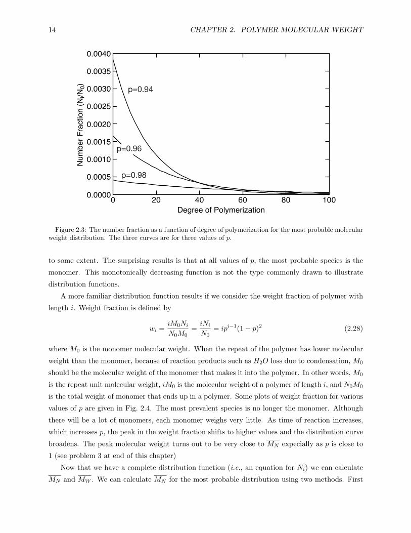
14 CHAPTER 2. POLYMER MOLECULAR WEIGHT
Degree of Polymerization
Num
ber F
ract
ion
(Ni/N
0)
0 20 40 60 80 100 0.0000
0.0005
0.0010
0.0015
0.0020
0.0025
0.0030
0.0035
0.0040
p=0.94
p=0.98
p=0.96
Figure 2.3: The number fraction as a function of degree of polymerization for the most probable molecularweight distribution. The three curves are for three values of p.
to some extent. The surprising results is that at all values of p, the most probable species is the
monomer. This monotonically decreasing function is not the type commonly drawn to illustrate
distribution functions.
A more familiar distribution function results if we consider the weight fraction of polymer with
length i. Weight fraction is defined by
wi =iM0Ni
N0M0=iNi
N0= ipi−1(1− p)2 (2.28)
where M0 is the monomer molecular weight. When the repeat of the polymer has lower molecular
weight than the monomer, because of reaction products such as H2O loss due to condensation, M0
should be the molecular weight of the monomer that makes it into the polymer. In other words, M0
is the repeat unit molecular weight, iM0 is the molecular weight of a polymer of length i, and N0M0
is the total weight of monomer that ends up in a polymer. Some plots of weight fraction for various
values of p are given in Fig. 2.4. The most prevalent species is no longer the monomer. Although
there will be a lot of monomers, each monomer weighs very little. As time of reaction increases,
which increases p, the peak in the weight fraction shifts to higher values and the distribution curve
broadens. The peak molecular weight turns out to be very close to MN expecially as p is close to
1 (see problem 3 at end of this chapter)
Now that we have a complete distribution function (i.e., an equation for Ni) we can calculate
MN and MW . We can calculate MN for the most probable distribution using two methods. First

2.6. MOST PROBABLE MOLECULAR WEIGHT DISTRIBUTION 15
Degree of Polymerization
Wei
ght F
ract
ion
(wi)
0 20 40 60 80 100 0.000
0.005
0.010
0.015
0.020
0.025
p=0.94
p=0.96
p=0.98
Figure 2.4: The weight fraction as a function of degree of polymerization for the most probable molecularweight distribution. The three curves are for three values of p.
we evaluate the sums in the number average molecular weight formula:
MN =∑∞
i=1 iM0Ni∑∞i=1Ni
= M0(1− p)∞∑i=1
ipi−1 (2.29)
The evaluation of the sum is nontrivial. The sum, however, can be expressed as the derivative of
another sum which is simpler to evaluate.
∞∑i=1
ipi−1 =d
dp
∞∑i=1
pi =d
dp
(p
1− p
)(2.30)
Evaluating the derivative gives∞∑i=1
ipi−1 =1
(1− p)2(2.31)
Multiplying by M0(1− p) gives
MN =M0
1− p(2.32)
An alternative and simpler method to MN is to realize that, by conservation of mass, the total
weight of material is always M0N0. From above, the total number of polymers is N0(1− p). Thus
MN =Total weight of polymer
Total number of polymers=
M0N0
N0(1− p)=
M0
1− p(2.33)

16 CHAPTER 2. POLYMER MOLECULAR WEIGHT
To get MW for the most probable distribution we use the weight average molecular weight
formula in terms of weight fractions:
MW =∞∑i=1
wiiM0 = M0(1− p)2∞∑i=1
i2pi−1 (2.34)
We evaluate the sum using the trick used to find MN and some additional work.
∞∑i=1
i2pi−1 =d
dp
∞∑i=1
ipi =d
dp
(p∞∑i=1
pi−1
)=
d
dp
(p
(1− p)2
)(2.35)
The last step uses the result from the MN calculation. Evaluating the derivative gives
∞∑i=1
i2pi−1 =1 + p
(1− p)3(2.36)
Multiplying by M0(1− p)2 gives the final result:
MW = M01 + p
1− p(2.37)
Combining the results for MN and MW , the polydispersity index for the most probable distri-
bution isMW
MN
= 1 + p (2.38)
As the reaction nears completion, p approaches one and the polydispersity index approaches 2.
That is the coefficient of variation of the most probable distribution is 100%. That large of a
coefficient of variation means that the molecular weight distribution is relatively broad.
We also notice that as p approaches one, both MN and MW approach infinity. This limit
means that all the monomers will be in a single polymer molecule. It is usually not desirable to
have molecular weights that are too high. Such polymers would not be processible; they would
not flow when melted. To avoid unprocessible polymers, it is desirable to use methods to control
molecular weight. One way to control molecular weight would be to freeze the reaction at some p
less than one. This scheme, however, can produce a material that is unstable with time. Instability
occurs if over long times, there are more reactions (albeit at a slow rate) which cause p to increase.
When p increases, the polymer properties change with time and might eventually give a molecular
weight that is too high to be processible.
One solution to molecular weight control is to polymerize the two monomers A A and B B
instead of the single monomer A B. If the two monomers are mixed in equal proportions, the
analysis will be identical to the one above and there will be no molecular weight control (note:
although the analysis is the same, the meaning of M0 has to be changed to be half the repeat
unit molecular weight to account for the fact that the synthesis is from two monomers (A−A and
2.6. MOST PROBABLE MOLECULAR WEIGHT DISTRIBUTION 17
B−B) instead of from one monomer (A−B)). If the proportions are unequal and r = NA/NB < 1
then the results are different. A more complicated analysis gives the following MN :
MN =M0(1 + r)1 + r − 2rp
≈ M0(1 + r)1− r
(2.39)
where, as explained above, M0 is half the repeat unit molecular weight. The second part of this
equation assumes p is equal to one. Sample calculations for various values of r give
r = 1.00 MN =∞r = 0.99 MN = 199M0
r = 0.95 MN = 39M0
r = 0.90 MN = 19M0
By selecting r, we see it is possible to control molecular weight to some finite value. Physically
what happens is that the monomer mixture runs out of A A and all polymers are end capped
with B B monomers. Because B can only react with A and no unreacted A remains, the reaction
stops at a finite molecular weight. The only problem is that small changes in r lead to large changes
in MN . For example a 5% deviation of r from 1.00 reduces the molecular weight from infinite to
39M0. But, 39M0 is not a very high molecular weight and may not be high enough to be useful.
To prevent polymerization from stopping at low molecular weights, you must have accurate control
over r. Also you must account for any side reactions and monomer volatility which might remove
monomer of one type and effectively change r.
Problems
2–1. Suppose you have n batches of polydisperse polymers. Let Ni,j be the number of polymers
of type j with degree of polymerization i and Mi,j be the molecular weight of that polymer.
The basic MN and MW equations for the total mixture of polymers now require double sums:
MN =
∑nj=1
∑iNi,jMi,j∑n
j=1
∑iNi,j
and MW =
∑nj=1
∑iNi,jM
2i,j∑n
j=1
∑iNi,jMi,j
(2.40)
Now, assume that the number average and weight average molecular weights of batch j are
MNj and MWj . and that you mix a weight wj of each batch to make a new polymer blend.
a. Starting from the above basic number average molecular weight definition, show that
the number average molecular weight of the blend is
MN =w1 + w2 + · · ·+ wn
w1
MN 1+ w2
MN 2+ · · ·+ wn
MNn
In other words, show that MN of the blend can be calculated from the individual MNj
of the components of the blend. Here MNj has the usual definition of
MNj =∑
iNi,jMi,j∑iNi,j
(2.41)

18 CHAPTER 2. POLYMER MOLECULAR WEIGHT
or a sum over just the polymers of component j.
b Starting from the above basic weight average molecular weight definition, show that the
weight average molecular weight of the blend is
MW =w1MW 1 + w2MW 2 + · · ·+ ωnMWn
w1 + w2 + · · ·+ wn
In other words, show that MW of the blend can be calculated from the individual MWj
of the components of the blend. Here MWj has the usual definition of
MWj =
∑iNi,jM
2i,j∑
iNi,jMi,j(2.42)
or a sum over just the polymers of component j.
2–2. Calcium stearate (Ca(OOC(CH2)16CH3)2, molecular weight = 607) is sometimes used as a
lubricant in the processing of poly(vinyl chloride). A sample of pure PVC polymer with a
polydispersity index of 2.8 is modifed by the addition of 3% by weight of calcium stearate.
TYhe mixture of PVC and salcium stearate is found to have MN = 15, 000 g/mol.
a. What is the MN of the PVC part of the compound? (Hint: use the blend MN result
from the previous problem.)
b. What is the MW of the blend?
c. What effect does the calcium stearate have on the light scattering and osmotic pressure
properties of the polymer? (Hint: light scattering measures MW while osmotic pressure
measures MN )
d. What is the highest possible MN for a polymer containing 3% by weight of calcium
stearate?
2–3. Consider the most probable molecular weight distribution:
a. Derive an expression for P (M) where P (M) is the probability that a randomly selected
polymer chain as molecular weight M . Express your result in terms of M (and not
degree of polymerization i).
b. What molecular weight has the maximum probability?
c. Derive an expression for w(M) where w(M) is the weight fraction of polymer that has
molecular weight M . Again, express your answer in terms of M (and not x).
d. What molecular weight has the largest weight fraction? Express your answer in terms
of the number average molecular weight.
2–4. Calculate the percentage conversion of functional groups required to obtain a polyester with
a number-average molecular weight of 24,000 g/mol from the monomer HO(CH2)14COOH.
2.6. MOST PROBABLE MOLECULAR WEIGHT DISTRIBUTION 19
2–5. A polyamide was prepared by bulk polymerization of hexamethyl diamine (9.22 g and molec-
ular weight 116) and adipic acid (13.2 g and molecular weight 166) at 280C. Analysis of the
whole reaction product showed that it contained 2.6× 10⁻³ moles of carboxylic acid groups.
Evaluate MN of the mixture. Assume it has a “most probable distibution” and also evaluate
MW .

20 CHAPTER 2. POLYMER MOLECULAR WEIGHT

Chapter 3
MOLECULAR CONFORMATIONS
3.1 Introduction
Polymers can exist in various conformations and various configurations. Two polymers which differ
only by rotations about single bonds are said to be two different conformations of that polymer.
A schematic view of two polymer conformations is show in Fig. 3.1. Two polymers which have the
same chemical composition but can only be made identical (e.g., superposable) by breaking and
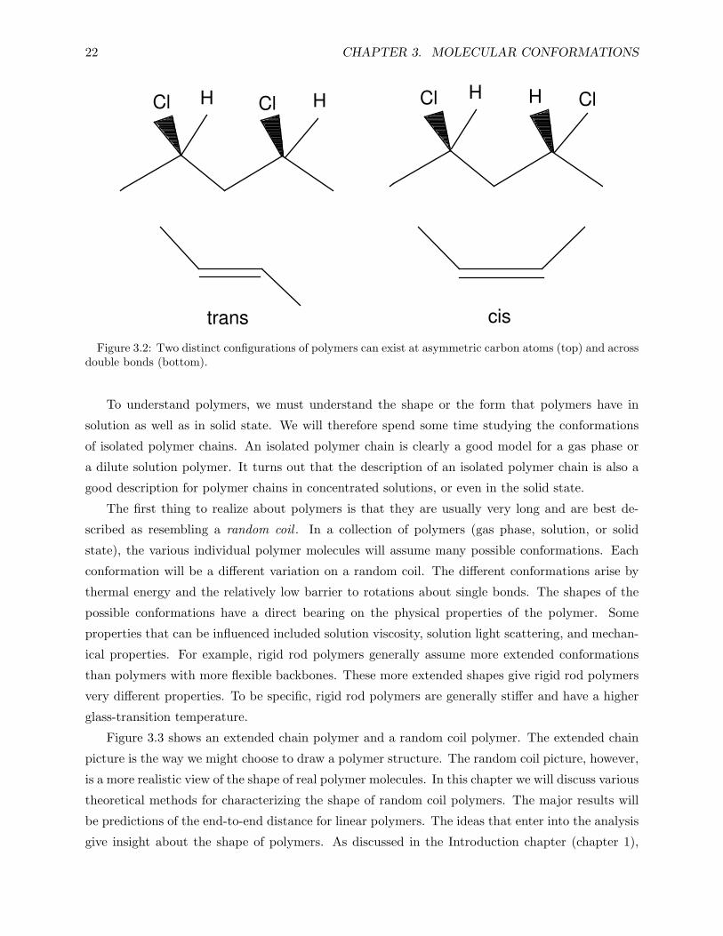
reforming bonds are said to be two configurations of that polymer. Two examples in Fig. 3.2 are
polymers that contain asymmetric carbon atoms or that contain double bonds. Asymmetric carbon
atoms can exist in d or l states while double bonds can exist in cis or trans states. No manner of
rotations about single bonds can turn polymers in different configuration states into superposable
polymers.
The above definitions of conformation and configuration are standard, but they have not always
been rigorously followed in the literature. For example, Paul Flory, who won a Nobel prize for
studies of polymer conformations, used configuration in his writings when he meant conformation.
Fortunately a writer’s meaning is usually obvious from context. It is recommended that you strive
to use the correct terminology as defined above. These notes strive to follow that convention.
Figure 3.1: Two molecules with different conformations. These two molecules can be made identical witha rotation of 180 about the central single bond.
21
22 CHAPTER 3. MOLECULAR CONFORMATIONS
Cl H Cl H Cl H H Cl
trans cisFigure 3.2: Two distinct configurations of polymers can exist at asymmetric carbon atoms (top) and across
double bonds (bottom).
To understand polymers, we must understand the shape or the form that polymers have in
solution as well as in solid state. We will therefore spend some time studying the conformations
of isolated polymer chains. An isolated polymer chain is clearly a good model for a gas phase or
a dilute solution polymer. It turns out that the description of an isolated polymer chain is also a
good description for polymer chains in concentrated solutions, or even in the solid state.
The first thing to realize about polymers is that they are usually very long and are best de-
scribed as resembling a random coil . In a collection of polymers (gas phase, solution, or solid
state), the various individual polymer molecules will assume many possible conformations. Each
conformation will be a different variation on a random coil. The different conformations arise by
thermal energy and the relatively low barrier to rotations about single bonds. The shapes of the
possible conformations have a direct bearing on the physical properties of the polymer. Some
properties that can be influenced included solution viscosity, solution light scattering, and mechan-
ical properties. For example, rigid rod polymers generally assume more extended conformations
than polymers with more flexible backbones. These more extended shapes give rigid rod polymers
very different properties. To be specific, rigid rod polymers are generally stiffer and have a higher
glass-transition temperature.
Figure 3.3 shows an extended chain polymer and a random coil polymer. The extended chain
picture is the way we might choose to draw a polymer structure. The random coil picture, however,
is a more realistic view of the shape of real polymer molecules. In this chapter we will discuss various
theoretical methods for characterizing the shape of random coil polymers. The major results will
be predictions of the end-to-end distance for linear polymers. The ideas that enter into the analysis
give insight about the shape of polymers. As discussed in the Introduction chapter (chapter 1),

3.2. NOMENCLATURE 23
Figure 3.3: Extended chain polymer on the left. A more realistic picture of a polymer as a random coil onthe right. The colors indicate rotation angle about each bond. Blue is for trans bonds while read and greenare for gauche bonds.
this type of polymer characterization is theoretical characterization.
3.2 Nomenclature
We will restrict ourselves to linear polymers and we will consider all their possible conformations.
To describe any given conformation we must first define a nomenclature or coordinate system. We
begin with a polymer having n bonds. These n bonds connect n+ 1 backbone atoms. We can thus
define any conformation by giving the 3(n+ 1) Cartesian coordinates of the n+ 1 atoms along the
polymer backbone. This nomenclature works but is normally more cumbersome than desired and
we thus make some simplifications.
We begin with the bond length (l). In many polymers the bonds in the polymer backbone are all
identical and therefore have a constant bond length. For example, in PE the bonds are all carbon-
carbon bonds and they are all typically about 1.53A long. For simplicity we will restrict ourselves
to polymers with constant bond lengths. A generalization to non-constant bond lengths can be
made later if necessary. With constant bond lengths, we can consider a polymer conformation as
a 3D random walk of n steps where each step has length l. Instead of listing absolute coordinates
of each atom in the backbone, we choose to describe a polymer by listing the relative directions of
each step in the random walk.
Directions in space are most conveniently described using polar angles. Figure 3.4 shows an
arbitrary direction in space emanating from the origin of a coordinate system. The angle with
respect to the z axis is called the polar angle and is usually denoted by θ. The angle that the

24 CHAPTER 3. MOLECULAR CONFORMATIONS
z
y
x
θ
φ
Figure 3.4: Definitions of the polar angle θ and the azimuthal angle φ for any vector in a right-handedcoordinate system.
projection of the direction onto the x–y plane makes with any consistently chosen reference point
in that plane is called the azimuthal angle and is usually denoted by φ. All possible directions in
space can be spanned by choosing θ from 0 to π and φ from 0 to 2π. In other words, any direction
from the origin can be defined by a unique pair of θ and φ.
We will represent a polymer as a 3D random walk of n steps where n is the number of bonds
(note that n is not necessarily the same as the degree of polymerization or the number of repeat
units; some repeat units have more than one bond and for n we count all of these bonds). In the
random walk, each step can be described by polar and azimuthal angles, θ and φ, where those
angles are given with respect to an axis system centered on the atom at the start of that bond. For
n bonds, each bond will have its own angles, θi and φi, and the complete chain will be described
with the 3 original coordinates for the first atom and the 2n angles for the steps of the random
walk. We thus require 2n+ 3 variables to specify a conformation of a polymer with constant bond
length.
Normally we will not be concerned with the absolute location in space of the polymer chain.
If we do everything relative to the location of the first bond, then we do not need to know the 3
original coordinates nor the 2 polar angles of the first bond. Subtracting these five variables, we can
define an arbitrary polymer conformation with 2n− 2 or 2(n− 1) variables. The 2(n− 1) variables
are the polar and azimuthal angles for each bond except the first bond. If we ever generalize to
different l’s for each bond, we must add to these 2(n− 1) variables, n new variables which specify
the length of each bond.

3.3. PROPERTY CALCULATION 25
φ=0˚
θi+1
φ=180˚
bond i+1
bond i
bond i-1
xz
l
φi+1
Figure 3.5: Definition of polar and azimuthal angles for bond i. With the illustrated selection of x, y, andz axes, the polar angle is the bond angle for bond i + 1 and the azimuthal angle is the dihedral angle forbond i+ 1.
It is convenient to choose a coordinate system that lends physical interpretations to the polar
and azimuthal angles of each bond in the polymer chain. As illustrated in Fig. 3.5, we consider
the central bond as bond i and take the z axis to point back along bond i. With this choice for
the z axis, the polar angle for bond i + 1 is just the bond angle between bond i and bond i + 1
(see Fig. 3.5). From now on, we will refer to the polar angle as the bond angle. The possible
orientations for bond i+ 1 when the bond angle is θi+1 sweep out the cone illustrated in Fig. 3.5.
The azimuthal angle (φ) for bond i+ 1 is the counter-clockwise angle around that cone from some
suitably selected reference point. We choose the x axis to define the reference point such that the
azimuthal angle for bond i + 1 is 180 when bond i is a trans bond. This choice is arbitrary, but
is consistent with the bulk of the modern literature (note: Flory choose φ = 0 to correspond to
trans bonds which makes his results shifted by 180 from these notes). Another term for such an
azimuthal angle is the dihedral angle for bond i+ 1 — a term that we will adopt throughout these
notes. Finally, the y axis is chosen to be perpendicular to the x and z axes and directed to make
the x-y-z coordinates a right-handed coordinate system.
3.3 Property Calculation
The goal of theoretical characterization of polymers is to be able to predict certain properties of
those polymers. When a polymer exists in a single conformation, the task is simple — we merely
calculate the property for that conformation. Random coil polymers, however, can exist in many
different conformations. An observed macroscopic property of an ensemble of polymer chains will
be an average value of that property over the range of polymer conformations. We denote the
average value of any property over an ensemble of random coil polymer chains as 〈Property〉.

26 CHAPTER 3. MOLECULAR CONFORMATIONS
The way to find 〈Property〉 is to examine a large number of polymer chains by considering
a large number of random walks. For the simplest models (models of short chains) we will be
able to examine all possible random walks. When we can consider all possible random walks we
can assign to each random walk a probability which equals the probability that that conformation
will be selected when one polymer is selected from an ensemble of random coils. Assuming we
can calculate some polymer property (e.g., size, stiffness, etc.) for each specific conformation, we
can average them to get the average of that property for the bulk polymer sample. The average
property is defined by
〈Property〉 =∑i
Property(conf i)× Probablity(conf i) (3.1)
where Property(conf i) is the value of the property calculated for conformation i and Probablity(conf i)
is the probability of that conformation occurring.
For small molecules you can often do the above averaging process exactly. In other words you
can enumerate all possible conformations, find the probability and property of each conformation,
and then find the average property by averaging the results. Some small molecules have only one
conformation and the task is relatively simple — the average property is equal to the property
of the single conformation. Other molecules have only a few conformations and the task is still
relatively simple. For a non chemistry example, consider the roll of a single dice and consider the
property of the number of pips showing on each role. A die has six faces which represent six possible
conformations of the die after each roll. When counting pips, the Property(conf i) = i. Assuming
the die is a fair die (i.e., not loaded) the probability of each conformation is the same and equal to
1/6 (thus Probablity(conf i) = 1/6). The property of the number of pips therefore has the exact
average value of
〈pips〉 =6∑i
i× 16
=16
+26
+36
+46
+56
+66
= 3.5 (3.2)
For polymer calculations there will usually be too many conformations to make the above
exact calculation procedure possible. Instead we will select conformations at random and use
a Monte Carlo procedure to get the average property. By the Monte Carlo procedure, if the
probability of selecting a particular conformation at random is proportional to the actual probability
of conformation i (selection probability ∝ Probablity(conf i)), than the average property for a
polymer sample can be approximated by
〈Property〉 ≈ 1N
∑Property(sample i) (3.3)
where N is the number of randomly generated polymer chains. The larger N , the more accurate
will be the calculated average property.
We can illustrate the Monte Carlo method with the dice problem. A Monte Carlo solution to
the dice problem would be to roll a die many times, total the pips, and divide by the number of
3.4. FREELY-JOINTED CHAIN 27
rolls. If the die was rolled sufficiently many times and if the die was fair (i.e., symmetric and not
loaded), the Monte Carlo solution would be very close to the exact answer of 3.5. After a few rolls,
the answer might differ from 3.5. After many rolls, however, the answer would be very unlikely to
show much deviation from 3.5.
The success of the Monte Carlo procedure is dependent on ones ability to select polymer confor-
mations with realistic probabilities that accurately reflect the true distribution of conformations.
This problem is easily solved in the dice problem by rolling a die. Unfortunately for polymer
problems we cannot physically select real polymers. Instead we have to generate conformations
mathematically or in a computer. The problem we must solve is the development of rules or al-
gorithms for realistically generating conformations. We will approach this problem in a series of
steps. We will begin with the simplest possible rules. At each subsequent step we will add more
realism to the procedure used to generate the random conformations. The final results can be used
to accurately predict many polymer properties.
3.4 Freely-Jointed Chain
In a freely-jointed chain all 2(n− 1) angular variables are allowed to assume any values with equal
probability. In others words the direction of any bond is equally likely to occur in any of the
possible directions of space — the joints at each bond thus move freely to allow all these possible
orientations.
Let’s begin with one particular property — the polymer size. Size can be characterized by
calculating the end-to-end distance, r, or the radius of gyration, s. As an average property, these
properties are usually calculated as a root mean squared end-to-end distance (or a root mean
squared radius of gyration). End-to-end distance is the distance from the beginning of the chain to
the end of the chain (see Fig. 3.6). The root mean squared end-to-end distance is the square root
of the average of the squared end-to-end distances:
rms r =√〈r2〉 =
√√√√ 1N
N∑i=1
r2i (3.4)
where N is the total number of possible conformations and ri is the end-to-end distance for confor-
mation i. The radius of gyration is the average of the distances of each of the atoms in the polymer
chain to the center of mass of the polymer. The root mean squared radius of gyration is the square
root of the average of the squared radius of gyrations:
rms s =√〈s2〉 =
√√√√ 1N
N∑i=1
s2i (3.5)
where si is the radius of gyration for conformation i.
28 CHAPTER 3. MOLECULAR CONFORMATIONS
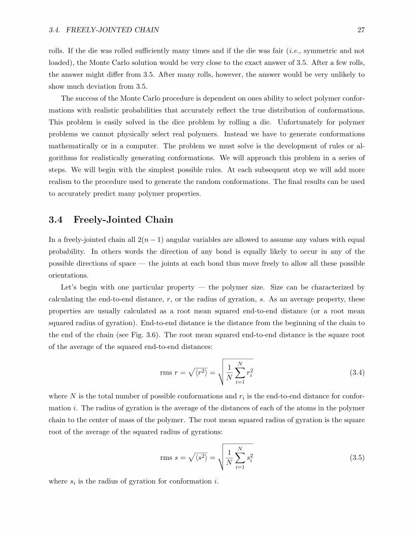
r
←
Figure 3.6: The length of a vector (~r) from the first atom to the last atom on a linear polymer chain isthe end-to-end distance for that polymer conformation. This figure shows the end-to-end vector.
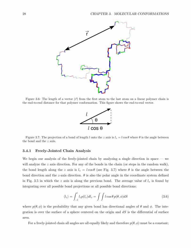
l
l cos θ
θ
Figure 3.7: The projection of a bond of length l onto the z axis is lz = l cos θ where θ is the angle betweenthe bond and the z axis.
3.4.1 Freely-Jointed Chain Analysis
We begin our analysis of the freely-jointed chain by analyzing a single direction in space — we
will analyze the z axis direction. For any of the bonds in the chain (or steps in the random walk),
the bond length along the z axis is lz = l cos θ (see Fig. 3.7) where θ is the angle between the
bond direction and the z-axis direction. θ is also the polar angle in the coordinate system defined
in Fig. 3.5 in which the z axis is along the previous bond. The average value of lz is found by
integrating over all possible bond projections or all possible bond directions:
〈lz〉 =∫ l
−llzp(lz)dlz =
∫ ∫l cos θ p(θ, φ)dS (3.6)
where p(θ, φ) is the probability that any given bond has directional angles of θ and φ. The inte-
gration is over the surface of a sphere centered on the origin and dS is the differential of surface
area.
For a freely-jointed chain all angles are all equally likely and therefore p(θ, φ) must be a constant;
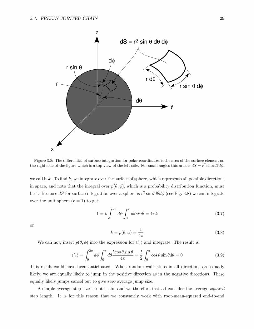
3.4. FREELY-JOINTED CHAIN 29
z
x
y
dφ
dθ
r
r sin θ
dS = r2 sin θ dθ dφ
r sin θ dφr dθ
Figure 3.8: The differential of surface integration for polar coordinates is the area of the surface element onthe right side of the figure which is a top view of the left side. For small angles this area is dS = r2 sin θdθdφ.
we call it k. To find k, we integrate over the surface of sphere, which represents all possible directions
in space, and note that the integral over p(θ, φ), which is a probability distribution function, must
be 1. Because dS for surface integration over a sphere is r2 sin θdθdφ (see Fig. 3.8) we can integrate
over the unit sphere (r = 1) to get:
1 = k
∫ 2π
0dφ
∫ π
0dθsinθ = 4πk (3.7)
or
k = p(θ, φ) =1
4π(3.8)
We can now insert p(θ, φ) into the expression for 〈lz〉 and integrate. The result is
〈lz〉 =∫ 2π
0dφ
∫ π
0dθl cos θ sin θ
4π=l
2
∫ π
0cos θ sin θdθ = 0 (3.9)
This result could have been anticipated. When random walk steps in all directions are equally
likely, we are equally likely to jump in the positive direction as in the negative directions. These
equally likely jumps cancel out to give zero average jump size.
A simple average step size is not useful and we therefore instead consider the average squared
step length. It is for this reason that we constantly work with root-mean-squared end-to-end

30 CHAPTER 3. MOLECULAR CONFORMATIONS
distances in our discussion of polymer size. Squaring each step length makes all step size positive
and we are guaranteed to get a nonzero result. With the known p(θ, φ) function, we can easily
calculate the mean squared jump size:
〈l2z〉 =∫ 2π
0dφ
∫ π
0dθl2 cos2 θ sin θ
4π=
l2
2
∫ π
0cos2 θ sin θdθ (3.10)
=l2
2
[−1
3cos2 θ
∣∣∣∣π0
]=l2
3(3.11)
The root mean squared distance per step is:√〈l2z〉 =
l√3
(3.12)
The above result gives as an average jump size per step, but we are concerned with the total
z axis root-mean-squared end-to-end distance. The solution to this problem is approached by
considering a set of typical jump directions. For a chain of n bonds, some of the bonds will point in
the positive z direction and some will point in the negative z direction. If n is large, the root mean
squared length of all positive jumps will be the same as that of all negative jumps and each will be
equal to the average of all jumps. We let n+ be the total number of jumps in the positive direction
and n− be the total number of jumps in the negative direction. Then the root-mean-squared
distance traveled in the z direction, denoted by z, is
z = (n+ − n−)√〈l2z〉 = (n+ − n−)
l√3
(3.13)
To solve for z we must determine (n+ − n−). The factor(n+ − n−) is like the result of a coin
toss experiment. Each step is considered a coin toss, if z increases on the step the coin toss result
is heads, if z decreases, the coin toss result is tails. In the coin toss results, the expected result is to
have equal numbers of heads and tails. If a large number of coin tosses are made the distribution
of (n+ − n−) will be a Gaussian function centered at zero (mean of zero). We can thus represent
the factor (n+ − n−), or more usefully the distance in the z direction, with the following Gaussian
distribution function:
W (z)dz =1√
2πσ2e−z22σ2 dz =
β√πe−β
2z2dz (3.14)
where σ is the standard deviation in z-direction distance and the term β is defined in terms of
standard deviation by
β =1√2σ2
(3.15)
The freely-jointed chain problem is solved if we can find the standard deviation in z-direction
distance. For a single step the variance, or the standard deviation squared, follows simply from the
formula for variance:
σ21 = 〈l2z〉 − 〈lz〉2 = 〈l2z〉 (3.16)
3.4. FREELY-JOINTED CHAIN 31
Statistical analysis tells us that for n steps, the standard deviation in z is n times the standard
deviation for a single step or
σ2 = nσ21 = n〈l2z〉 (3.17)
Substituting the above result for 〈l2z〉 gives
β =1√
2n〈l2z〉=
√3
2nl2(3.18)
An alternate route to finding β is to find the variance by integration (i.e., find the average value
of z2 and subtract the square of the average value of z, which we know to be zero). The result is
〈z2〉n
= 〈l2z〉 =λ2
3=
1n
∫ ∞−∞
z2W (z)dz =1
2nβ2(3.19)
Solving for β again gives
β =
√3
2nl2(3.20)
The expression for β together with the Gaussian distribution function give the distribution
function for chain length in one direction. Now we need to solve the three-dimensional problem.
Because the chain is freely jointed, the three axes are independent of each other. From probability
theory, the probability that a given polymer chain jumps distances of x, y, and z in each of the three
Cartesian directions is the product of the probabilities for each of the axes considered separately.
The probability that a chain has an end-to-end distance characterized by a vector (x, y, z) is thus
W (x, y, z)dx dy dz = W (x)W (y)W (z)dx dy dz (3.21)
Because the analysis for W (z)dz given above applies equally well to the x and y directions, we have
W (x, y, z)dx dy dz =(β√π
)3
e−β2r2dx dy dz (3.22)
where r2 = x2 + y2 + z2 is the square of the distance from the origin to the end of the chain at
(x, y, z).
As stated above, W (x, y, z)dx dy dz gives the probability that a chain’s end-to-end vector is
characterized by a vector (x, y, z). In other words, it is the probability that a chain that begins at
the origin ends in a box center at the point (x, y, z) or size dx dy dz (see Fig. 3.9). One dimension of
W (x, y, z)dx dy dz is plotted in Fig. 3.9. The function is a Gaussian distribution function centered
at the origin or centered about the mean value of zero.
The function W (x, y, z)dx dy dz solves the freely-jointed chain problem, but it is not in the most
useful form. We are normally not concerned with absolute end of the chain (i.e., location (x, y, z)),
but rather with the end-to-end distance r. To find this result we sum up all possible (x, y, z)
coordinates that give the same r value. In other words, we integrate over the volume element V

32 CHAPTER 3. MOLECULAR CONFORMATIONS
z
y
x
dV = dx dy dz
βr-3 -2 -1 0 1 2 3
0.0 0.1 0.2 0.3 0.4 0.5 0.6 0.7 0.8 0.9 1.0
Figure 3.9: The left side shows a chain that starts at the origin and ends in a box centered a (x, y, z). Theright side is a one-dimensional plot of W (x, y, z)dx dy dz.
of width dr where√x2 + y2 + z2 is between r and r + dr. The volume element of constant r is
a spherical shell as shown in Fig. 3.10. Integrating over this volume element yields a probability
distribution in terms of the end-to-end distance r:
W (r)dr =∫VW (x, y, z)dx dy dz =
(β√π
)3
4πr2e−β2r2dr (3.23)
This type of distribution function is called a radial distribution function.
Figure 3.11 schematically plots the end-to-end distance distribution function, W (r)dr. We can
characterize the distribution function by finding some key points. The function W (r)dr always
increases to some maximum and then decrease towards zero. The peak value is found by finding
where the derivative of W (r)dr is zero. The maximum value, rmax, occurs at
rmax =1β
= l
√2n3
= 0.82l√n (3.24)
The average value of r, 〈r〉, is found by integrating W (r)dr:
〈r〉 =∫ ∞
0rW (r)dr =
2β√π
= l
√8n3π
= 0.92l√n (3.25)
Likewise, the mean-squared value of r, 〈r2〉, is
〈r2〉 =∫ ∞
0r2W (r)dr =
32β2
= l2n (3.26)
and the root mean squared end-to-end distance is√〈r2〉 = l
√n (3.27)

3.4. FREELY-JOINTED CHAIN 33
z
y
x
← ←
r + dr
←
rShell ofwidth dr
Figure 3.10: Cross section of a spherical shell between radii of r and r + dr.
length (units of l √n)
W(r
) dr
0.0 0.5 1.0 1.5 2.0 2.5 3.0 0.0
0.1
0.2
0.3
0.4
0.5
0.6
0.7
rmax = 0.82 l √n<r> = 0.92 l √n
<r2> = l √n√
Figure 3.11: A typical plot of W (r)dr. The key values rmax, average r or 〈r〉, and root-mean-squared rare indicated on the figure.

34 CHAPTER 3. MOLECULAR CONFORMATIONS
The above key values are indicated in Fig. 3.11. For constant l and n, they always rank in the
order rmax < 〈r〉 < 〈r2〉.The variance in the end-to-end distance can be found from the mean and mean-squared end-
to-end distances:
σ2 = 〈r2〉 − 〈r〉2 =3
2β2− 4β2π
=0.23β2
= 0.15nl2 (3.28)
From this results, the coefficient of variation (standard deviation divided by the mean) is
CV =σ
〈r〉= 42% (3.29)
This result can be characterized as a fairly large coefficient of variation.
3.4.2 Comment on Freely-Jointed Chain
We only used two facts in deriving W (r). First we assumed that the chain can be simulated by a
random walk. Second, we assumed there are enough steps to make the random walk a Gaussian
distribution. To find the Gaussian curve we therefore only had to find the mean (mean = 0) and the
standard deviation (σ =√n〈l2z〉). The final result predicts that the root-mean-squared end-to-end
distance is √〈r2〉 = l
√n (3.30)
In other words the root mean squared end-to-end distance is proportional to the square root of the
number of bonds and linear in the bond length.
The linear dependence on bond length is a trivial result. It is merely a scaling parameter.
Thus if we double all bond lengths we double the end-to-end distance. It can also be thought of
as a consequence of units. If we solve the problem in inches and then in millimeters, we should
get answers that differ only by the units conversion factor for inches to millimeters of 25.4. This
expected result will only occur if the end-to-end distance is linear in bond length.
The dependence of root-mean-squared end-to-end distance on the square root of the number of
bonds is a profound, or at least a non-trivial, result. Let’s consider the origins of the square root
dependence on bond length. Our analysis is one of a completely random three dimensional random
walk. The square root of n dependence comes from the expression for the standard deviation of
the walk which contains√n. If we repeated the analysis for one- or two-dimensional random walks
we would find the same result. The root-mean-squared end-to-end distance is√〈r2〉 = l
√n (3.31)
in any dimension. We thus conclude that the square root of n dependence is a property of the
random walk nature of polymers and unrelated to geometrical effects. Only polymer features that
alter the random walk nature of the chain can alter the square root dependence on n.

3.4. FREELY-JOINTED CHAIN 35
Walk to the right
Walk to the left
...
...
Figure 3.12: The only two possible one-dimensional, self-avoiding random walks.
To anticipate a future result that does alter the random walk nature of polymers, we consider
self-avoiding random walks. In self-avoiding random walks, the path cannot revisit any spot that
was previously visited. Because no two atoms in a polymer chain can occupy the same space,
a self-avoiding random walk is a better model for a polymer chain than the completely random
walk discussed previously. A self-avoiding random walk, however, is not a completely random walk
because some steps may be influenced by previous steps. In other words, some steps may be biased
away from moving in a given direction because doing so would revisit a previous part of the random
walk.
The exact analysis of two- and three-dimensional self-avoiding random walks is not possible.
One-dimensional, self-avoiding random walks, however, are trivial to analyze. As shown in Fig. 3.12
there are only two possible one-dimensional, self-avoiding random walks. A one-dimensional random
walk must begin with one step to the left or to the right. If the first step is to the left, the next step
must also be to the left because a step to the right would revisit the starting location. Continuing
on, the chain that starts to the left must make all steps to the left. The other possible chain is the
one that starts with its first step to the right. This chain can only continue with repeated steps
to the right. There are thus only two possible chains. One makes all n steps to the left and its
length is nl. The other makes all n steps to the right and its length is also nl. Averaging over
all possible chain conformations, the root-mean-squared end-to-end distance for a one-dimensional,
self-avoiding random walk is √〈r2〉 = nl (3.32)
In contrast to the completely random walk, this result is now linear in n. Because of scaling
requirements it remains linear in l.
In two- and three-dimensional random walks, the effect of imposing self avoiding characteristics
will be less dramatic. A one-dimensional, self-avoiding, random walk is hardly random. All steps
(except the first one) are determined by the requirement of being self avoiding and not by random
chance. Two- and three-dimensional, self-avoiding random walks will not restricted as much. Some
steps will be influenced by self-avoiding requirements, but most will have other options than can
be reached by random chance. Without proof, we state that the end-to-end distance for two- and
three-dimensional random walks will be proportional to n to some power between 0.5 and 1.0.
The two extremes are completely random walks (power equal to 0.5) and self-avoiding random

36 CHAPTER 3. MOLECULAR CONFORMATIONS
walks in which every step is determined by the self-avoiding requirement (power of 1.0). The
former extreme is the random walk result from above; the later extreme is the one-dimensional,
self-avoiding random walk result.
We now return to the random walk analysis and its assumption that the polymer chains are
long enough such that a Gaussian distribution function accurately represents the results. How big
do the chains have to be to be large enough? The Gaussian distribution was applied to the factor
(n+ − n−). For large chains with random n+ and n− jumps, we require |n+ − n−| n. W (r)dr is
accurate as long as this inequality is true. W (r)dr, however, is supposed to work for all values of
r which includes r near rmax = nl. The maximum value of r can only occur when all jumps are in
the same direction which means either n+ = n and n− = 0 or n− = n and n+ = 0. In each of these
cases |n+ − n−| = n and the requirement that |n+ − n−| be much less than n is violated. In other
words, as r gets large, the chain becomes less Gaussian and W (r)dr becomes increasing inaccurate.
To assess the accuracy of W (r)dr, some researchers have constructed more detailed analyses
that account for deviations from Gaussian behavior at large r. One published result is
W (r)dr = (Const)4πr2 exp
−β2r2
[1 +
310
(r
rmax
)2
+ . . .
]dr (3.33)
The first term within the square brackets is 1 which is the previous result for a Gaussian distribution.
The rest of the terms within the square brackets are correction terms that are small for small r
and become more significant for large r. Only the first and largest correction term is given. Let’s
consider a chain of n bonds and say that the uncorrected W (r)dr is adequate as long as the
correction term is less than 0.01 (or less than 1%). W (r)dr will then be good for a chain that is
up to f times larger than the root-mean-squared end-to-end distance (i.e., good for r ≤ f√〈r2〉)
as long as
310
(f√〈r2〉
rmax
)2
=3f2
10n< 0.01 or f =
√n
30(3.34)
For example consider a chain of n = 100 bonds (a fairly short polymer chain). Solving this
equation for f results in f = 1.83. Therefore the first correction term in W (r)dr is less than 1% for
0 < r < 1.83l√n = 18.3l. When 18.3l < r < nl = rmax = 100l the first correction term is greater
than 1%.
We can relate the range of small correction terms to the standard deviation in root mean
squared end-to-end distance. The upper limit in r for small corrections is fl√n where l
√n is the
root mean squared end-to-end distance. From above, the standard deviation in end-to-end distance
is 0.15l√n. Therefore the upper limit in r for small corrections is
fl√n− l
√n
0.15l√n
=
√n30 − 10.15
(3.35)
standard deviations above the mean. For the above example with n = 100 bonds, this equation
shows the W (r)dr is accurate as long as r is less than 5.50 standard deviations above the mean. In
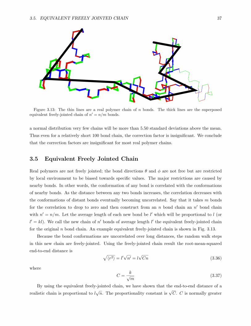
3.5. EQUIVALENT FREELY JOINTED CHAIN 37
Figure 3.13: The thin lines are a real polymer chain of n bonds. The thick lines are the superposedequivalent freely-jointed chain of n′ = n/m bonds.
a normal distribution very few chains will be more than 5.50 standard deviations above the mean.
Thus even for a relatively short 100 bond chain, the correction factor is insignificant. We conclude
that the correction factors are insignificant for most real polymer chains.
3.5 Equivalent Freely Jointed Chain
Real polymers are not freely jointed; the bond directions θ and φ are not free but are restricted
by local environment to be biased towards specific values. The major restrictions are caused by
nearby bonds. In other words, the conformation of any bond is correlated with the conformations
of nearby bonds. As the distance between any two bonds increases, the correlation decreases with
the conformations of distant bonds eventually becoming uncorrelated. Say that it takes m bonds
for the correlation to drop to zero and then construct from an n bond chain an n′ bond chain
with n′ = n/m. Let the average length of each new bond be l′ which will be proportional to l (or
l′ = kl). We call the new chain of n′ bonds of average length l′ the equivalent freely-jointed chain
for the original n bond chain. An example equivalent freely-jointed chain is shown in Fig. 3.13.
Because the bond conformations are uncorrelated over long distances, the random walk steps
in this new chain are freely-jointed. Using the freely-jointed chain result the root-mean-squared
end-to-end distance is √〈r2〉 = l′
√n′ = l
√Cn (3.36)
where
C =k√m
(3.37)
By using the equivalent freely-jointed chain, we have shown that the end-to-end distance of a
realistic chain is proportional to l√n. The proportionality constant is
√C. C is normally greater

38 CHAPTER 3. MOLECULAR CONFORMATIONS
than one and therefore√C is sometimes called the expansion factor and sometimes denoted as α.
It tells how much the real chain is expanded relative to a freely jointed chain. The square of the
expansion factor, or C, is known as the characteristic ratio. It is defined by
C =〈r2〉nl2
(3.38)
In the freely-jointed chain, C = 1. In real polymers the characteristic ratio is a function of n or
the number of bonds and is usually greater than 1. It is customary to write the bond-dependent
characteristic ratio as Cn. In relatively ideal polymers Cn approaches a limiting constant value for
large n. The value of Cn at large n for such polymers characterizes the random coil nature of that
polymer. Low values of Cn correspond to tightly coiled polymers and high values of Cn correspond
to polymers that are loosely coiled or extended.
In real polymers, self-avoiding requirements or excluded volume effects, to be described latter,
cause Cn to increase without bound as n increases without bound. A scaling law derived by
deGennes states that for large n, Cn increases in proportion to n0.2. Thus we have
Cn =〈r2〉nl2∝ n0.2 (3.39)
or √〈r2〉 ∝ ln0.6 (3.40)
This result agrees with the previous discussion of self-avoiding random walks which claimed that
the power-law dependence on n for a real chain is between 0.5 (for a completely random chain) and
1.0 (for a chain with all steps controlled by self-avoiding requirements).
Our discussion on the equivalent freely-jointed chain shows that any real polymer can be reduced
to any expression for end-to-end distance that is proportional to l√n (provided we ignore, for the
moment, excluded volume effects). The thing that distinguishes one polymer from another is
the characteristic ratio C. We thus embark on a series of models whose main purpose is to use
theoretical arguments for calculating the characteristic ratio.
3.6 Vector Analysis of Polymer Conformations
We will find it useful to develop an alternate approach to the analysis of end-to-end distance in
polymers. The new analysis will be based on vectors and analytical geometry. We associate with
each bond a vector. Let the vectors ~u1 to ~un be the vectors along the n bonds. Then a vector from
one end of the chain to the other is simple the sum of these vectors:
~r =n∑i=1
~ui (3.41)

3.6. VECTOR ANALYSIS OF POLYMER CONFORMATIONS 39
The mean squared end-to-end distance is
〈r2〉 = 〈~r · ~r〉 = 〈n∑i=1
~ui ·n∑j=1
~uj〉 (3.42)
Expanding this expression for a polymer chain with a constant bond length, i, results in
〈r2〉 =n∑i=1
~ui · ~ui + 2∑i<j
〈~ui · ~uj〉 (3.43)
where the sum over i < j means all combinations of i and j such that i is less than j. The factor of
2 in front of the sum includes, by symmetry, the terms when i is greater than j. The dot product
of a vector with itself is simply the square of the length of the vector. Thus we can write
〈r2〉 = nl2 + 2l2∑i<j
〈cos θ′ij〉 (3.44)
where θ′ij is the angle between the vectors along bond j and along bond i. If vector j is equal to
i+ 1 (i.e., the bond next to bond i) then θ′ij is the supplement of the bond angle between bonds i
and i+ 1.
For the freely-jointed chain, the bond directions are uncorrelated and 〈cos θ′ij〉 is zero which
yields√〈r2〉 = l
√n as before. This result was obtained with less work than the previous analysis.
The previous analysis, however gave a full distribution function (a Gaussian distribution) while this
one only gives the root-mean-squared end-to-end distance. For more complicated models, we will
need to evaluate the term 〈cos θ′ij〉.We can use a vector analysis to investigate the relation between end-to-end distance and radius
of gyration - s. In vector notation, we can write an expression for s2 in which ~ri is the location of
the ith atom along the polymer chain and ~z is the location of the center of mass:
s2 =1n
∑i
(~ri − ~z) · (~ri − ~z) (3.45)
Expanding this sum results in
ns2 =∑i
r2i + nz2 − 2~z ·∑i
~ri (3.46)
where ri is the distance from the origin to atom i and z is the distance from the origin to the center
of mass. The definition of the center of mass is
~z =1n
∑i
~ri or∑i
~ri = n~z (3.47)
Substituting this expression in to the above results gives
ns2 =∑i
r2i − nz2 =∑i
r2i − n(~z · ~z) =∑i
r2i −1n
∑i
∑j
~ri · ~rj (3.48)

40 CHAPTER 3. MOLECULAR CONFORMATIONS
ririj
rj
rij2 = ri
2 + rj2 - 2 ri rj cos θ
Figure 3.14: A triangle framed by vectors ~ri and ~rj . The vector ~rij connects the two ends of vectors ~riand ~rj .
To evaluate the vector dot product ~ri · ~rj , consider the triangle in Fig. 3.14. By the cosine law
the length of the vector ~rij connecting the ends of vectors ~ri and ~rj is
r2ij = r2i + r2j − 2rirj cos θ = r2i + r2j − 2~ri · ~rj (3.49)
Solving for ~ri · ~rj gives
~ri · ~rj =r2i + r2j − r2ij
2(3.50)
The expression for the radius of gyration then simplifies to:
s2 =1
2n2
∑j
∑i
r2ij =1n2
∑j
∑i<j
r2ij (3.51)
In this step we made use of symmetry (rij = rji) and the fact that rii = 0.
Because the vectors ~ri are the coordinates of the atoms in the polymer chain, the distance rijis the end-to-end distance for a sub-polymer chain of j − i bonds. By the discussion in the section
on the equivalent freely-jointed chain, we can write this distance as
r2ij = C(j − i)l2 (3.52)
We do not know the value of C but it is the characteristic ratio for the polymer under consideration
and may depend on j − i (especially for small j − i). Ignoring the j − i dependence of C, inserting
this result, and reordering the summation over i yields:
s2 =Cl2
n2
n∑j=1
j−1∑i=1
i =Cl2
n2
n∑j=1
j(j − 1)2
≈ Cl2
2n2
n∑j=1
j2 =Cl2
2n2
n(n+ 1)(2n+ 1)6
(3.53)
For large polymer chains (large n) this result simplifies to
√〈s2〉 =
√Cnl2
6=
√〈r2〉
6(3.54)
We conclude that whenever 〈r2〉 = Cnl2 for a polymer, that the radius of gyration is directly
proportional to (and smaller than) the end-to-end distance. This result holds for large molecules

3.7. FREELY-ROTATING CHAIN 41
when Cn is independent of n. An important corollary to this result is that everything we learn
while studying the end-to-end distance also applies to the radius of gyration. The reverse is also
true. Any analysis or experiments that give us information about the radius of gyration also give
us information about the end-to-end distance.
The approximations used to relate radius of gyration to end-to-end distance can be understood
using a matrix representation. Using the equivalent freely-jointed chain approximation, the radius
of gyration squared is the sum of all terms above the diagonal of the following matrix:
0 Cl2 2Cl2 3Cl2 4Cl2 . . .
− 0 Cl2 2Cl2 3Cl2 . . .
− − 0 Cl2 2Cl2 . . .
− − − 0 Cl2 . . .
− − − − 0 . . .
. . . . . . . . . . . . . . . . . .
(3.55)
The terms near the diagonal are random walk, long-chain approximations for short chains and may
be inaccurate. If the matrix is large, however, there will be many more terms far from the diagonal
then close to the diagonal. For large matrices, the inaccuracies in the terms close to the diagonal
will have only a negligible effect on the sum of all terms. Thus the relation between 〈s2〉 and 〈r2〉derived above will be accurate. In order for the derived relation, rewritten here as
〈r2〉〈s2〉
= 6 (3.56)
to be accurate, the chain must be slightly larger than is required for 〈r2〉 to be equal to Cnl2.
The relation will be inaccurate for short chains or for chains that are not random walk coils (e.g.,
extended chain polymers).
3.7 Freely-Rotating Chain
Commonly the bond angles in polymers are fixed or narrowly fixed to constant values. For example,
in polyethylene the bonds angles are all close to 112. It takes much more energy to distort bond
angles than it does to induce rotations about single bonds. We therefore consider a random walk
where all bond angles, θi, are constant and equal to one value θ. The more easily moved dihedral
or rotational angles are considered to all be equally likely. Thus there is free rotation about each
bond and hence we call this model the “freely-rotating chain” model. The conformation of a given
chain is reduced to specifying the dihedral angles for n− 1 bonds (all bonds except the first bond).
To analyze the freely-rotating chain we use the vector approach outlined in the previous section.
By taking successive projections of one bond onto another, we can show (See Flory book) that
〈cos θ′ij〉 = cosm θ′ where m = |j − i| where θ′ = π − θ is the supplement of the fixed bond angle.

42 CHAPTER 3. MOLECULAR CONFORMATIONS
The resulting vector analysis becomes
〈r2〉 = nl2 + 2l2i<j∑
cosj−i θ′ (3.57)
This expression can be imagined as the sum of all the terms in the matrix of size n × n in which
the element at row i and column j is cos|j−i| θ′:
l2 ×
1 cos θ′ cos2 θ′ cos3 θ′ . . . cosn−1 θ′
cos θ′ 1 cos θ′ cos2 θ′ . . . cosn−2 θ′
......
......
......
cosn−1 θ′ cosn−2 θ′ . . . cos2 θ′ cos θ′ 1
(3.58)
The n diagonal terms sum to n which give the first term (nl2) in the 〈r2〉 expression. Writing out
the required terms for the summation term by inspection of this matrix gives
〈r2〉 = nl2 + 2l2[(n− 1) cos θ′ + (n− 2) cos2 θ′ + . . .+ (n− (n− 1)) cosn−1 θ′
](3.59)
which can be written as
〈r2〉 = nl2 + 2l2n−1∑i=1
(n− i) cosi θ′ (3.60)
We rewrite this summation in simpler terms by letting x = cosθ′:
〈r2〉 = nl2 + 2l2 (nS1 − xS2) (3.61)
where
S1 =n−1∑i=1
xi and S2 =n−1∑i=1
ixi−1 (3.62)
The terms S1 and S2 can be evaluated in closed form for all values of n. For polymer problems,
we are normally concerned with large n for which these sums converge to constant values and we
can treat the two sums as infinite series. The infinite geometric series S1 has the well known result
S1 ≈∞∑i=1
xi = x(1 + x+ x2 + x3 + . . .
)=
x
1− x(3.63)
For S2, we use a trick by noticing that
S2 =d
dx
n−1∑i=1
xi =dS1
dx(3.64)
For large n we thus have
S2 ≈d(
x1−x
)dx
=1
(1− x)2(3.65)

3.8. HINDERED ROTATING CHAIN 43
Substituting S1 and S2 into the expression for 〈r2〉 gives
〈r2〉 = nl2 + 2l2[nx
1− x− x
(1− x)2
](3.66)
For large n, the second term in the brackets quickly becomes negligible and we have
〈r2〉 = nl2 +2nl2x1− x
= nl21 + x
1− x(3.67)
Finally we substitute for x and note that cos θ = − cos θ′ (where θ is the bond angle and θ′ = π− θis the supplement of the bond angle). We get
〈r2〉 = nl21− cos θ1 + cos θ
(3.68)
The root-mean-squared end-to-end distance for large, freely-rotation chains is
√〈r2〉 = l
√n
√1− cos θ1 + cos θ
(3.69)
The characteristic ratio is
Cn =〈r2〉nl2
=1− cos θ1 + cos θ
(3.70)
Note that the characteristic ratio is independent of n. This independence is a consequence of our
assumption of large n. It is possible to evaluate S1 and S2 for any value of n and get an exact
result. The exact result gives a Cn that depends on n but rapidly converges to the above result for
large n.
For an example we consider polyethylene. All carbon bonds are in approximately tetrahedral
geometries. We can thus approximate all bond angles by the tetrahedral angle of θ = 109.47or
cos θ = −1/3 (note: it is easier to remember the tetrahedral angle as the cos−1(−1/3) than it is to
remember it as 109.47). For a freely-rotating polyethylene chain√〈r2〉 = l
√2n (3.71)
and the characteristic ratio is Cn = 2. Real polyethylene is not totally symmetric and thus the
C C C bonds deviate slightly from 109.47 to 112. The C C H and H C H bonds shrink
slightly to compensate. This slight increase in bond angle increases the characteristic ratio by 10%
to Cn = 2.20.
3.8 Hindered Rotating Chain
The dihedral angle is clearly not free to assume all possible values. Instead the angle is restricted
by steric interactions. Consider the potential energy for rotation about the central C C bond in
butane (CH3 CH2 CH2 CH3) shown in Fig. 3.15. The rotations about the central C C bond

44 CHAPTER 3. MOLECULAR CONFORMATIONS
Rotational Angle
Ene
rgy
0 60 120 180 240 300 360 0
1
2
3
4
C
C
C
H
HH
H
φ
Figure 3.15: Left side is an end view of the central C–C bond in butane. The right side plots to potentialenergy as a function of angle with φ = 180 defined as the trans position illustrated on the left side.
in butane are a reasonable model for the C C rotations in polyethylene. A preferred analogy
would be higher molecular weight alkanes. Those experiments and their analysis have been done,
but with more effort and less accuracy than available for butane.
The trans state illustrated on the left side of Fig. 3.15 is the lowest energy state. It is lowest
because the two CH3 groups, which are larger than the H atoms, are as far apart as possible. As
rotations occur the groups appended to each of the central C atoms come into closer proximity and
the steric energy increases. There are local maxima at φ = ±120. These maxima occur when the
CH3 groups are aligned with H atoms on the other carbon atom. There are local minima when
φ = ±60. These minima occur when all the groups are staggered (as in the left of Fig. 3.15) but
the CH3 groups are adjacent to each other rather than opposite each other as in the trans state.
These local minima are called the gauche+ and gauche- states. Finally there is a local maximum
at φ = 0, which occurs when the two CH3 groups on either end of the butane chain are aligned
and as close together as possible.
When rotations are hindered by potential energy functions such as those shown in Fig. 3.15,
it is clear that the rotations will not be free. All rotational angles are perhaps possible, but the
dihedral angles will have a preference for the low energy states. For butane, most bonds will be
at or near the trans state (φ = 180) or at or near the local gauche minima (φ = ±60). Thermal
energy will allow the angles to deviate from these states and to overcome the barriers to transitions
from one state to another. The populations of all rotational angles, however, will not be equal. We
thus replace the freely-rotating chain with a more realistic hindered-rotating chain model.
End-to-end distance for a hindered-rotation chain is more difficult to find than the freely-

3.9. MORE REALISTIC ANALYSIS 45
rotating chain model. We omit the details and give the results. The final equation is found using
the vector analysis and averaging the dot products ~ui ·~uj , while accounting for unequal populations
of the possible rotational angles. The result is
√〈r2〉 = l
√n
√1− cos θ1 + cos θ
√1− 〈cosφ〉1 + 〈cosφ〉
(3.72)
where 〈cosφ〉 is the average value of the rotational angle. The characteristic ratio is
Cn =〈r2〉nl2
=1− cos θ1 + cos θ
1− 〈cosφ〉1 + 〈cosφ〉
(3.73)
Note that if this hindered-rotation chain becomes freely-rotating chain then 〈cosφ〉 = 0 and the
results reduce to the freely-rotating chain results.
For a detailed example, let’s consider polyethylene with l = 1.53A, n = 5000 bonds, and
θ = 112. The simplest model, the freely-jointed chain model, gives√〈r2〉 (freely jointed) = 108A (3.74)
and a characteristic ratio of 1. The next most realistic model, the freely-rotating chain model, gives√〈r2〉 (freely rotating) = 108
√2.20A = 160A (3.75)
and a characteristic ration of 2.20. For the hindered-rotation chain model we need to know 〈cosφ〉.We thus need some new information. For example, we will say that experiments show that 60% of
the bonds have φ = 180 (trans) and 20% each have φ’s of +60 or −60 (gauche+ or gauche-).
Then the average dihedral angle gives
〈cosφ〉 = −0.6 + 0.2× (0.5) + 0.2× (0.5) = −0.4 (3.76)
The end-to-end distance for the hindered-rotation chain is√〈r2〉 (hindered rotation) = 108
√2.20√
2.33A = 245A (3.77)
and the characteristic ratio is Cn = 5.13. We can compare this result to the experimental result
for polyethylene which is 6 to 7 (depending on temperature). The hindered rotating chain gives
a result that is close to the correct results, but is still too low. In the next section we consider
improvements on the hindered rotating chain model.
3.9 More Realistic Analysis
We can list two general factors that influence the end-to-end distance, but are not included in the
hindered rotation chain model — short range interactions and long range interactions. The next
step in our analysis is to include some, or preferable all, of these effects.

46 CHAPTER 3. MOLECULAR CONFORMATIONS
We consider short-range interactions as interactions with neighboring bonds that affect the
relative probabilities of the dihedral angle. When we include short range interactions we cannot
take a simple average of cosφ as in the hindered rotation model. We need to account for the effect
of neighboring bonds. In its simplest implementation we might assume that the conformation of
one bond depends on relative energies that are influenced by the conformation of the previous
bond. Each step of the random walk then requires an adjustment of the jump-direction proba-
bilities according to the conformation of the previous bond. Some probability analysts call such
models Markov chains instead of random walks. After we develop a model that does a good job
of accounting for short-range interactions, we will have a good model for polymer conformations
that are unperturbed by the long-range interactions described below. We will call the polymers
generated by this modified random walk or Markov chain process “unperturbed polymer conforma-
tions.” The end-to-end distance of these chains will be called the unperturbed end-to-end distance
and will be denoted with a subscript zero — 〈r2〉0.
Long-range interactions are all interactions that are not short-range interactions. To be more
specific, long-range interactions are interactions between atoms or molecular units that are not
covalently bonded to each other. Defined this way, long range interactions include interactions
between two parts of the polymer that are separated by many bonds or between the polymer and
solvent molecules. We discuss three types of long-range interactions.
The first important perturbation to random walks is that while random walks can cross their
own path, a polymer conformation cannot — random walks used to simulate polymer chains should
be self-avoiding random walks. This new feature is called the effect of excluded volume. The
elements of the chain exclude other elements from their occupied volume. If included in the analysis,
excluded volume will perturb the end-to-end distance and cause it to increase. Besides increasing
the end-to-end distance, excluded volume will cause the root-mean-squared end-to-end distance to
no longer be proportional to√n. When excluded volume effects are significant, we can assume
that 〈r2〉 is proportional to some power of n such as p (where p > 0.5):
〈r2〉 ∝ npl2 (3.78)
According to deGennes, p = 1.2 and therefore the characteristic ratio increases as n0.2:
Cn =〈r2〉nl2∝ n0.2 (3.79)
A second long-range interaction is interactions between the polymer and the solvent. A solvent
can cause the unperturbed end-to-end distance to increase or decrease. A good solvent will cause
it to increase. In effect the polymer will prefer interactions with the solvent over interactions with
itself and therefore will expand to maximize polymer-solvent interactions. A poor solvent will cause
the unperturbed end-to-end distance to contract. The polymer wants to avoid the solvent and thus
will contract on itself to avoid polymer-solvent interactions. In the extreme case, a poor solvent will
3.10. THETA (Θ) TEMPERATURE 47
cause the polymer to completely contract and precipitate out of solution. This extreme example of
a poor solvent is better characterized as a non-solvent.
The last types of long-range interactions are specific interactions. By specific interactions we
mean identifiable interactions between remote parts of the chains. Two examples are hydrogen
bonding and ionic interactions.
After considering both short-range and long-range interactions we are led to split the problem of
theoretical polymer characterization into two parts. The first part is the study of the unperturbed
end-to-end distance. We plan to modify the hindered rotation chain model to correctly account for
short-range interactions and thereby calculate the correct unperturbed end-to-end distance. After
solving this problem we will consider what influence the long-range interactions (including excluded
volume effects) have on the results. Let’s define α to be the factor by which the linear dimension
expands (α > 1) or contracts (α < 1) due to long-range interactions:√〈r2〉 = α
√〈r2〉0 (3.80)
The solution to the long-range interaction problem is to find α.
3.10 Theta (Θ) Temperature
We also need to consider temperature effects. Temperature can affect all types of interactions.
It can affect short-range interactions by influencing the relative probabilities of the various dihe-
dral angles. Rotations about single bonds are influenced by the presence of thermal energy and
thus higher temperature will make it more likely to find conformations in higher-energy rotational
angles. Temperature affects long-range interactions mainly through polymer-solvent interactions.
In general increasing the temperature improves solvent quality and lowering it decreases solvent
quality.
As discussed in the previous section, we will first attempt to solve the short-range interaction
problem. The first problem we encounter is how do we know when we have the right answer? Real
polymers have long-range interactions and short-range interactions. Thus real polymers have a
mean-squared end-to-end distance of 〈r2〉 and not 〈r2〉0. If we compare our theoretical analysis to
experimental results we will normally find disagreement, regardless of whether the analysis to find
〈r2〉0 was correct or not. Fortunately there is an experimental solution to this problem called the
theta (Θ) temperature. For any given polymer-solvent pair, there is a specific temperature, called
the Θ temperature, for which the true end-to-end distance is equal to the unperturbed end-to-end
distance. Thus experiments at the Θ temperature can be used to measure 〈r2〉0 which can be
compared to experimental predictions.
The concept of Θ temperature can be understood by considering the effect of temperature
on polymer-solvent interactions. In general the polymer-solvent interactions for a given polymer-
48 CHAPTER 3. MOLECULAR CONFORMATIONS
solvent pair is an increasing function of temperature. As the polymer-solvent interaction increases
the solvent becomes a better solvent. Thus increasing temperature leads to a better solvent and to
a higher α; decreasing temperature leads to a poorer solvent and a lower α. For a given polymer-
solvent pair, there will be some temperature for which α = 1. That temperature is called the theta
(Θ) temperature. At the Θ temperature 〈r2〉 = 〈r2〉0 and experiments at the Θ temperature can
be used to measure 〈r2〉0.
Besides measuring 〈r2〉0, the Θ temperature has other useful properties. At the Θ temperature,
some physical properties (e.g., osmotic pressure) obey ideal laws up to high concentrations. Thus
simple theories for analysis of a physical property that do not account for long-range interactions
will still work well at the Θ temperature. There is an analogy between the Θ temperature and the
Boyle point of a gas. The Boyle point is the temperature where the repulsion between gas molecules
due to excluded volume is exactly compensated by their mutual attraction. At the Boyle point,
the ideal gas laws are obeyed to very high pressures. Note that conformity to ideal laws is one way
of determining the Θ temperature. The temperature can be varied until the measurements obey
ideal laws. That temperature is the Θ temperature.
Despite the advantages of the Θ temperature, we note that working in theta solvents is often
impractical. To get α down to one, you need a solvent that is sufficiently poor. The solvent may
become so poor the precipitation becomes imminent. It is often better to work in a good solvent
and correct the results to the unperturbed results. For measurements of physical properties, this
correction involves correcting ideal laws for large molecules or long-range interactions.
3.11 Rotational Isomeric State Model
The rotational isomeric state model will be our solution to the problem of accounting for short-range
interactions and some long range interactions (e.g., the effect of excluded volume). In general, any
polymer conformation is defined by a set of bond lengths, li, bond angles, θi, and dihedral angels,
φi. In the rotational isomeric state model, we assume that the polymer is restricted to certain
types of conformations or to certain isomeric states. Bond lengths are likely to vary only ±3% and
thus as before we consider them to be fixed at l. Likewise, bond angles are likely to vary only ±5
degrees and we consider them to be fixed at θ. The dihedral angles are not allowed to assume any
possible angle, but instead are assumed to be restricted to a small number of discrete values. The
possible discrete dihedral angles define the set of rotational isomeric states for each bond.
We will illustrate with polyethylene. These ideas will be extended to other polymers latter.
Due to symmetry of polyethylene there are three possible rotational isomeric states (see Fig. 3.16).
The trans state (φ = +180), the gauche+ state (φ = +60) and the gauche- state (φ = −60).
In the rotational isomeric state model, each bond of polyethylene is assumed to be in one of these
three states. No other values of φ are allowed. In reality, thermal fluctuations about the minima in

3.11. ROTATIONAL ISOMERIC STATE MODEL 49
C
C
C
H
H
H
H
C
C
C
H
HH
H
C
C
C
H
H
H
H
Trans Gauche -Gauche +Figure 3.16: The three rotational isomeric states in polyethylene. The dihedral angle, φ, is defined as the
angle between to white circles.
potential energy will lead to a distribution in φ’s around these three local minima. The rotational
isomeric state model asserts that we can realistically simulate a polymer chain by ignoring variations
in φ around the local minima.
In our random walk analysis of the rotational isomeric state, the probability of any bond existing
in one of the rotational state i characterized by angle φi, is given by a Boltzman factor:
P (φi) =e−E(φi)/RT
Z(3.81)
where Z is a normalizing factor or the sum of the Boltzman energy factors for all possible angles:
Z =3∑i=1
e−E(φi)/RT (3.82)
where E(φi) is the energy associated with the state at dihedral angle φi and the sum is over the
three possible states in Fig. 3.16 (Note: this equation can easily be generalized to more than three
rotational isomeric states) Because of short-range interactions discussed above, this probability
factor is expected to be affected by neighboring bonds. The simplest model is to assume that the
energy, E(φi), is affected by the bond conformation of the previous bond. This important nearest-
neighbor interaction is ignored in the hindered rotation chain model. Its inclusion in the rotational
isomeric state model is the major advance in realism in this new model.
To account for nearest neighbor interactions, we must consider all bond pairs and all possible
conditional probabilities of the form P (φi|φi−1), which gives the conditional probability that bond
i has angle φi given that the previous bond or bond i − 1 has angle φi−1. By analogy with the
previous probability factor
P (φi|φi−1) =e−E(φi−1φi)/RT
Z(φi−1)(3.83)

50 CHAPTER 3. MOLECULAR CONFORMATIONS
where Z(φi−1) is a normalizing factor or the sum of the Boltzman energy factors for all angles φigiven that φi−1 is fixed:
Z =3∑j=1
e−E(φi−1φj)/RT (3.84)
In these equations, E(φi−1φi) is the energy associated with two consecutive bonds with dihedral
angles φi−1 and φi. In this section we are restricting ourselves to three rotational states of trans
(t), gauche+ (g+), and gauche- (g−). The energy factors we care about are E(tt), E(tg+), E(tg−),
etc.. The conditional probabilities we are concerned with can conveniently be tabulated in a matrix
called the weighting factor matrix. For polyethylene (or for any three-state polymer) we write can
write a weighting factor matrix as
U =
P (t|t) P (g+|t) P (g−|t)P (t|g+) P (g+|g+) P (g−|g+)
P (t|g−) P (g+|g−) P (g−|g−)
(3.85)
For example, the matrix element P (t|g+) gives the probability that the next bond is trans given
that the previous bond was gauche+.
Let’s begin with the first row and arbitrarily assign the tt state to the ground state. Thus we
assume E(tt) = 0. The tg+ and tg− bond pairs will each be higher in energy than the tt bond pair.
In polyethylene, the excess energy associated with the two possible gauche bonds will be the same.
We let that excess energy be Eg or the extra energy associated with a gauche bond. We further
define
σ = e−Eg/RT (3.86)
and we can quickly derive Z(t) = 1 + 2σ and
P (t|t) =1
1 + 2σP (g+|t) =
σ
1 + 2σP (g−|t) =
σ
1 + 2σ(3.87)
Z(t) appears in the denominator of each probability as a normalizing factor.
For the second row, we might just consider the energy associated with all the gauche bonds
and assume E(g+t) = Eg and E(g+g+) = E(g+g−) = 2Eg. The probabilities would become
P (t|g+) =σ
σ + 2σ2P (g+|g+) =
σ2
σ + 2σ2P (g−|g+) =
σ2
σ + 2σ2(3.88)
This simple analysis ignores an important short-range interaction that occurs when two consecutive
bonds are g+g− or g−g+. Figure 3.17 illustrates a g+g− conformation. Two parts of the polymer
chain separated by four bonds are in close proximity which causes a large steric interaction. This
interaction is known as the pentane effect and causes the energy of g+g− or g−g+ conformations to
be much higher than that g+g+ or g−g− conformations. If we let Ep be the energy of the pentane
effect interaction then E(g−g+) = 2Eg + Ep whereas E(g+g+) = 2Eg. Defining
ω = e−Ep/RT (3.89)

3.11. ROTATIONAL ISOMERIC STATE MODEL 51
C C
C
CC
Gauche -
Gauche +
StrongStericInteractions
Figure 3.17: The steric interactions caused by the pentane effect when two consecutive bonds are g+|g−or g−|g+.
we derive the conditional probabilities for the second row of U to be
P (t|g+) =σ
σ + σ2 + σ2ω=
11 + σ + σω
(3.90)
P (g+|g+) =σ2
σ + σ2 + σ2ω=
σ
1 + σ + σω(3.91)
P (g−|g+) =σ2ω
σ + σ2 + σ2ω=
σω
1 + σ + σω(3.92)
Analyzing the third row similarly to the second row and collecting all probabilities in the matrix
we arrive at
U =
1
1+2σσ
1+2σσ
1+2σ1
1+σ+σωσ
1+σ+σωσω
1+σ+σω1
1+σ+σωσ
1+σ+σωσω
1+σ+σω
(3.93)
It usually suffices to work with relative probabilities rather than absolute probabilities. By conven-
tion we normalize each row to the first element in that row. For a simple polymer like polyethylene,
we write the weighting matrix of relative probabilities as
U =
1 σ σ
1 σ σω
1 σω σ
(3.94)
By theory and experiment, the energy terms for polyethylene are well known. The best results give
Eg = 2100 J and Ep = 8400 J. At 300C these lead to weighting factors of
σ = e−2100J/RT = 0.43 and ω = e−8400J/RT = 0.081 (3.95)
Thus gauche bonds are only about 46% as likely as trans bonds (2σ/(1 + 2σ)) and g+|g− confor-
mations are only about 2.4% as likely (σω/(1 + σ + σω)).

52 CHAPTER 3. MOLECULAR CONFORMATIONS
We next consider how to use the rotational isomeric state model to predict polymer properties.
Imagine a polymer chain of n bonds. A polymer conformation of this chain is determined by setting
the states of each bond; each bond can be t, g+, or g−. We can ignore the first two bonds and thus
we need to set the states of the terminal n−2 bonds. The first bond can be ignored because it only
serves to locate the start of the polymer in space. The second bond direction is determined by the
rotational state of bond 1, but this state only serves to locate the initial direction of the random
walk. The remaining n− 2 bonds need to be determined.
There are two possible solutions to the rotational isomeric state model. Because each bond
has a small number of discrete states, the total number of polymer conformations is finite. For
a polymer with n bonds of which each bond can be in one of three states, the total number of
polymer conformations is 3n−2. One possible approach is to enumerate all possible conformations
and calculate properties using the exact process discussed earlier in this chapter. This exact solution
can be done for small n, but soon becomes impractical for large n’s typical of real polymers.
When n is large the total number of conformations is too large to enumerate, even on the fastest
supercomputer.
For large polymers, a preferred approach is to use the Monte Carlo method. We generate a large
number of chains using a random walk or Markov chain process. For each bond the probabilities of
the next bond being in a given state are determined by the weighting matrix like the one given above
and by the state of the previous bond. For each chain we can calculate a property of interest (e.g.,
end-to-end distance, radius of gyration, etc.). The average value of that property after generating
sufficiently many chains will be our Monte Carlo solution to the problem.
The above Monte Carlo random walk process requires a computer. The computer program
LatticeTM discussed in class is an example of a program that can do Monte Carlo simulations using
the rotational isomeric state model. Programs like LatticeTM are, in effect, computer experiments.
You set polymer properties by selecting weighting factors, excluded volume, temperature, etc..
Then you run the program and calculate the end-to-end distance or the radius of gyration. These
computer experimental results can be compared to real experimental results. If the two results
agree, you have evidence that the rotational isomeric state is a valid model for polymers. Fur-
thermore the physical concepts of the rotational isomeric state model give you insight about the
polymer molecules and the factors that control conformations.
The following pseudo computer code is the program logic, or flow chart, of the main part of
any program that does Monte Carlo solutions using the rotational isomeric state model. This flow
chart assumes a three rotational isomeric states, but it could easily be generalized to handle any
number of states.
let v = (1,0,0) or the first bond is t
for bond=2 to number of bonds-1

3.11. ROTATIONAL ISOMERIC STATE MODEL 53
let q=Uv be a vector giving the probabilities for t, g+, and g-
pick a random number between 0 and q1+q2+q3
if (random number is between 0 and q1) then
next bond is t and v = (1,0,0)
else if (random number is between q1 and q2) then
next bond is g+ and v = (0,1,0)
else if(random number between q2 and q3) then
next bond is g- and v = (0,0,1)
end if
if desired, check for excluded volume effects
if jump to occupied site, try another site, reject the entire
chain, or reject several previous bonds
if all sites occupied start new chain
end if
next bond
Now have set of n-2 bond conformations which completely define the chain
Calculate properties (e.g. end-to-end distance, radius of gyration, etc.)
Start over with another chain and continue until results converge
The key part of this loop is calculating the properties of each generated chain. You can calculate
any property than can be reliably calculated for a given polymer conformation. The simplest
and most reliable properties are size properties. The program LatticeTM calculates the following
properties:
1. Last r (end-to-end distance of current chain)
2. rms r
3. 〈r〉
4. rms s
5. r2
nl2— the characteristic ratio (equal to Cn)
6. r2
s2— how close is it to 6?
7. % trans
8. Number of rejected steps
9. Relative entropy

54 CHAPTER 3. MOLECULAR CONFORMATIONS
In addition to the above calculations, LatticeTM can also plot many results. It can plot each
generated polymer in a three-dimensional view. These stick figures give a feel for typical polymer
conformations. It can plot the distribution of end-to-end distances and compare them to the radial
Gaussian function calculated for in the freely-jointed chain analysis.
There is one important aspect of LatticeTM and many rotational isomeric state solutions that
requires discussion. As implied by its name, LatticeTM generates chains on a tetrahedral lattice.
This requires all bonds angles to be the tetrahedral bond angle of 109.47. Because it is a regular
lattice, it also requires all bonds lengths to be the same. This type of simulation is reasonably
accurate for polyethylene and for many other carbon-backbone polymers. Lattice simulations,
however, cannot give you information about the effect of bond angle (e.g., 112 in real polyethylene
vs. the 109.47 in a tetrahedral lattice) and cannot simulate polymers with different bond lengths.
The advantage of lattice simulations is that they are fast. They can do most of the work with
integer arithmetic which is much faster in computers. The use of a lattice makes it possible to do
meaningful simulations in personal computers such as Macintoshes. An off-lattice calculation on a
Macintosh would be limited to much more rudimentary work and to much shorter chains.
We can simulate many polymers using the rotational isomeric state model. Some interesting
polymers are:
1. Polyethylene (see above)
2. Polytetrafluoroethylene (PTFE)
3. Copolymers
4. Polyoxymethylene (POM) (Delrin, Celcon, etc.)
5. Polypropylene (PP) — a vinyl polymer
Some results from these types of polymers are discussed in the LatticeTM manual and will be covered
in class.
Problems
3–1. The radial distribution function for the freely-jointed chain model was shown in class to be
W (r)dr =(β√π
)3
4πr2e−β2r2dr (3.96)
where
β =
√3
2nl2(3.97)
Because the form of the radial distribution function even for non-freely-jointed chains is similar
to the freely-jointed chain result (except with a different value for β) it is worth studying this
function.

3.11. ROTATIONAL ISOMERIC STATE MODEL 55
a. Show that the maximum in W (r)dr occurs at r = 1β
b. Show that the mean value of r is 〈r〉 = 2β√π
.
c. Show that the average value of r2 is 〈r2〉 = 32β2
d. What is the standard deviation in r?
e. Express the answers to a through d in terms of number of bonds (n) and bond length
(l).
3–2. Pretend that linear polyethylene (PE or (CH2 CH2)n ) can be modeled as a freely-jointed
chain in which each bond is 1.53A long. Using the results from problem 2-1, evaluate the
following quantities:
a. How many bonds are in a 500,000 g/mole PE polymer chain?
b. What is the maximum length of the chain?
c. What is the most likely end to end distance?
d. What is the mean end-to-end distance
e. What is the root mean squared end-to-end distance?
f. What is the standard deviation in r?
g. Plot the radial distribution function for this polymer chain and indicate on your plot
the answers to c, d, and e.
3–3. Polymer A contains x freely jointed segments each of length la and polymer B contains y
freely jointed segments each of length lb. One end of A is connected to one end of B to form
a two block, block copolymer.
a. What is the root-mean-squared end-to-end distance of this block copolymer?
b. If segments of A are randomly interspersed with segments of B and the segments are still
freely jointed, what would be the root-mean-squared end-to-end distance of the random
copolymer?
3–4. How do each of the following affect the radius of gyration?
a. Decreasing the molecular weight.
b. Decreasing the polymer-solvent interaction.
c. Adding the effects of excluded volume.
d. Reducing the hindrance to rotations about bonds.

56 CHAPTER 3. MOLECULAR CONFORMATIONS
3–5. Many polymers have more than one type of bond the different types of bonds may have
more the one value for bond length. One example is Nylon 66 whose repeat unit structure is
HO–C–(CH2)4–C–OH + H2N–(CH2)6–NH2
—(N–C–(CH2)4–C–N–(CH2)6)—
O O
O O
H H
This polymer has N–CH2 bonds, N–carbonyl bonds, carbonyl-CH2 bonds, and CH2–CH2
bonds. Explain, in general terms, how you would use the rotational isomeric state model to
calculate the characteristic ratio of Nylon 66.

Chapter 4
RUBBER ELASTICITY
4.1 Introduction
The mechanical properties that define a rubber elastic material are:
1. High elongation (often 5-10× or more elongation before failure)
2. Much of the elongation is recoverable (it returns to its original shape when unloaded)
3. The force required to elongate is low
Many polymers exhibit such rubber elasticity over some range in temperatures. Those polymers
that exhibit rubber elasticity at room temperature are caller elastomers. Furthermore, it is only
polymeric materials that can be elastomers (with some commercially-unimportant exceptions in
inorganic gels). Since the main unique feature of polymers is that they are large molecules, it is
logical to assume that rubber elasticity is a potential property of large, covalently bonded molecules.
But, what is it about polymers that makes it possible for them to be elastomers? What are the
mechanical properties of elastomers? How does one design new and improved elastiomers? Those
questions are discussed in this chapter.
4.2 Historical Observations
Rubbery materials have been around longer than the polymer industry. The first commercial
use of rubbers was developed by Charles Goodyear in 1830’s. He invented the process of rubber
vulcanization2 that converted natural rubber to a true elastomer with properties suitable for his
intended use as rubberized fabric. His “invention” is now an important part of polymer science.
At the time, however, researchers did not even understand the existence of polymer molecules. He
discovered vulcanization by chance and it was used for many years before its scientific basis became
clear.
57

58 CHAPTER 4. RUBBER ELASTICITY
Weight
Rubber
Heat
Figure 4.1: A specimen of rubber loaded under a constant weight and then heated. Upon heating thespecimen decreases in length.
Prior to vulcanized rubber, natural rubber from various sources existed and was studied in the
literature. In 1805, John Gough described a series of experiments on caoutchouc or Indian rubber.3
His first experiment was to monitor the temperature during elongation. He did not have elaborate
equipment, but was able to observe a temperature rise by stretching a rubber and bringing the
specimen into contact with his lips:
“For the resin evidently grows warmer the further it is extended; and the edges of the
lips possess a high degree of sensibility, which enables them to discover these changes
with greater facility than other parts of the body.”
The expectation for an elastic material (i.e., a material that recovers its shape when unloaded), is
that all the energy put into a specimen is stored as mechanical energy and then recovered when the
sample is unloaded. During such reversible unloading, it is unexpected to experience heat. Thus,
the behavior or rubber is unusual compared to other materials. Even though rubber increases in
temperature on elongation, it is still able to be reversible because it cools when unloaded.
Gough’s second experiment was to hang a weight on a piece of rubber (i.e., load a piece of
rubber at constant force) and then heat the specimen (see Fig. 4.1). The result of heating was that
the sample decreased in length. All other types of materials get slightly longer when heated due to
thermal expansion. In fact even a piece or rubber will thermally expand when it is not under load.
Rubber specimens under load, however, have the unusual property of getting shorter when heated.
Gough’s final experiments where to stretch rubber samples under water at different tempera-
tures. The elastomeric nature of the rubbers was preserved in warm water but was impaired in
cold water. It is not ususual for the elongation of materials to depend on temperature, but rubbery
materials depend dramatically on temperature. In fact the rubber elasticity effects disappear at
sufficiently low temperature. A common science demonstration is to bounce a rubber ball, dip it in
liquid nitrogen, and then show that it shatters like glass when bounced again. This effect is loss of
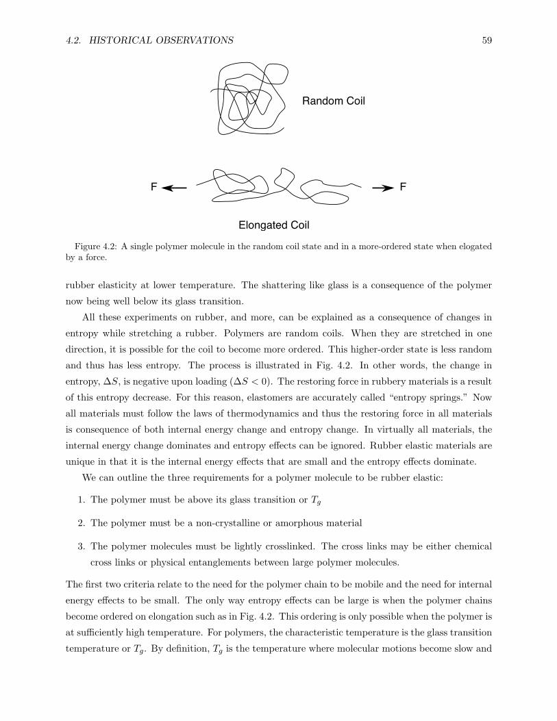
4.2. HISTORICAL OBSERVATIONS 59
Random Coil
F F
Elongated Coil
Figure 4.2: A single polymer molecule in the random coil state and in a more-ordered state when elogatedby a force.
rubber elasticity at lower temperature. The shattering like glass is a consequence of the polymer
now being well below its glass transition.
All these experiments on rubber, and more, can be explained as a consequence of changes in
entropy while stretching a rubber. Polymers are random coils. When they are stretched in one
direction, it is possible for the coil to become more ordered. This higher-order state is less random
and thus has less entropy. The process is illustrated in Fig. 4.2. In other words, the change in
entropy, ∆S, is negative upon loading (∆S < 0). The restoring force in rubbery materials is a result
of this entropy decrease. For this reason, elastomers are accurately called “entropy springs.” Now
all materials must follow the laws of thermodynamics and thus the restoring force in all materials
is consequence of both internal energy change and entropy change. In virtually all materials, the
internal energy change dominates and entropy effects can be ignored. Rubber elastic materials are
unique in that it is the internal energy effects that are small and the entropy effects dominate.
We can outline the three requirements for a polymer molecule to be rubber elastic:
1. The polymer must be above its glass transition or Tg
2. The polymer must be a non-crystalline or amorphous material
3. The polymer molecules must be lightly crosslinked. The cross links may be either chemical
cross links or physical entanglements between large polymer molecules.
The first two criteria relate to the need for the polymer chain to be mobile and the need for internal
energy effects to be small. The only way entropy effects can be large is when the polymer chains
become ordered on elongation such as in Fig. 4.2. This ordering is only possible when the polymer is
at sufficiently high temperature. For polymers, the characteristic temperature is the glass transition
temperature or Tg. By definition, Tg is the temperature where molecular motions become slow and

60 CHAPTER 4. RUBBER ELASTICITY
difficult. Thus whenever T > Tg molecular motions are easy and rubber elasticity is possible. The
requirement to be an amorphous material is similar. A crystalline structure is not mobile and
deformations of crystals result in internal energy changes that impair rubber elasticity. The last
criteria is less obvious. The need for cross linking is to make the material a solid rather than a liquid.
After all, many materials are highly mobile and non-crystalline but are still not rubber elastic; they
are liquids. To be rubber elastic, a liquid-like material has to be cross linked to prevent viscous
flow. It is the cross links that allow the material to recover when unloaded. Goodyear’s invention
of vulcanization was actually an invention of a process for cross linking natural rubber. Natural
rubber, in its native state, is slightly crystalline and too fluid for significant commercial uses. By
cross linking using vulcanization, the crystallinity disappears and the mechanical properties become
much more useful. Finally, it is the need for cross linking that makes polymers the only materials
that can be elastomers. They are the only liquid-like materials that can be readily cross linked.
4.3 Thermodynamics
The deformation of elastomers and how they differ from most other materials can be understood
by simple (albeit non-rigorous) thermodynamics analysis for uniaxial loading. The first law of
thermodynamics is
dQ+ dW = dU (4.1)
where dQ is heat added to the sample, dW is work done on the sample, and dU is the change in
internal energy. (Note that chemical engineers frequently define work done by a sample and thus
the dW term changes sign. In mechanics, it is more natural to think in terms of work done on a
sample). In a reversible process (such as loading an elastic material), the heat term is dQ = T dS
where T is absolute temperature and dS is the change in entropy. The work term is
dW = Fd`− P dV (4.2)
The first term is work of extension (force F times distance of extension or change in length d`). The
second term is expansion work, but it is generally very small during uniaxial loading. Substitution
into the first law of thermodynamics gives
T dS + Fd` = dU + P dV = dH (4.3)
where dH is the enthalpy change (by definition dH = dU + P dV ). Finally, solve for the force of
elongation gives
F =(∂H
∂`
)T,P
− T(∂S
∂`
)T,P
(4.4)
The first term in the extension force is the force due to enthalpy change, which is very close
to the internal energy change (since P dV is small). For nearly all engineering materials, such as

4.3. THERMODYNAMICS 61
metals, ceramics, polymers (with T < Tg), etc., this first term dominates as the force is equal to
the internal energy change per unit length change. For elastomers, however, the converse is true.
The internal energy change is small while the entropy change is large. Thus for elastomers, the
force of extension is
F ≈ −T(∂S
∂`
)T,P
(4.5)
Because extension (∂` > 0) causes a decrease in entropy (∂S < 0), the negative sign is correct
and leads to a positive force. Conventional engineering materials and elastomers are two extremes
of the force equation in which one of the two terms dominates. It is possible for materials to be
between these two extremes where the internal energy and entropy terms are of similar magnitude,
but such materials are uncommon.
To explain temperature effects in Gough’s experiments3 requires slightly more advanced ther-
modynamics. The free energy change, dG, on extension is:1
dG = V dP − S dT + Fd` (4.6)
Using reciprocity relations in thermodynamics, this relation leads to
−(∂S
∂`
)T,P
=(∂F
∂T
)`,P
(4.7)
Thus, when an elastomer is stretched (∂` > 0) causing the entropy to decrease (∂S < 0), the left
hand side (with the minus sign) is positive. This result implies that whenever the force increases
(∂F > 0) that the temperature must increase too (∂T > 0). This relation thus explains Gough’s
first experiment. Gough’s second experiment is length as a function of temperature at constant
force. This experiment can be explained by more involved thermodynamics,1 but will not be
discussed here.
Actually, Eq. (4.7) is true for any material, but it is only elastomers for which the decrease
in entropy is sufficient to cause an easily observable temperature increase. Equation (4.7) gives
a simple experiment to verify this dominant role of entropy in elastomers. The experiment is to
measure force as a function of temperature at constant length and pressure. The slope of the results
is (∂F/∂T )`,P , which by Eq. (4.7) is equal to −(∂S/∂`)T,P . Substitution of this entropy result into
Eq. (4.4) provides simultaneous measurement of enthalpy (or approximately internal energy) change
during elongation. The results for such experiments on elastomers and conventional materials are
shown schematically in Fig. 4.3. For elastomers, the slope is large and positive and the energy
terms can be shown to be small. For most other materials the slope is close to zero. As shown in
Fig. 4.3, most materials have a slightly negative slope due to thermal expansion. As the material
expands when held at fixed length, it expands against the grips and therefore reduces the force.
Such experiments can prove the dominance of entropy effects in elastomers and their absence in
other materials.
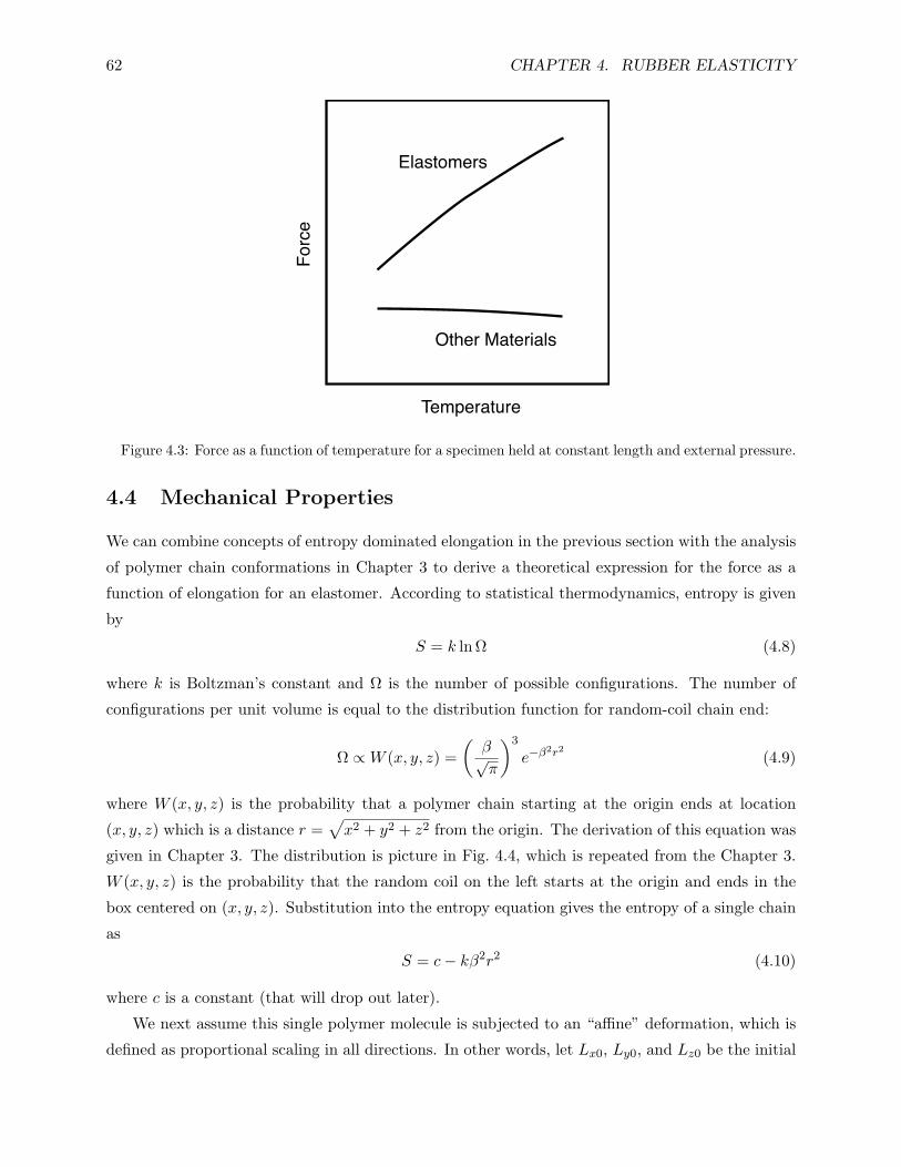
62 CHAPTER 4. RUBBER ELASTICITY
Temperature
Forc
e
Elastomers
Other Materials
Figure 4.3: Force as a function of temperature for a specimen held at constant length and external pressure.
4.4 Mechanical Properties
We can combine concepts of entropy dominated elongation in the previous section with the analysis
of polymer chain conformations in Chapter 3 to derive a theoretical expression for the force as a
function of elongation for an elastomer. According to statistical thermodynamics, entropy is given
by
S = k ln Ω (4.8)
where k is Boltzman’s constant and Ω is the number of possible configurations. The number of
configurations per unit volume is equal to the distribution function for random-coil chain end:
Ω ∝W (x, y, z) =(β√π
)3
e−β2r2 (4.9)
where W (x, y, z) is the probability that a polymer chain starting at the origin ends at location
(x, y, z) which is a distance r =√x2 + y2 + z2 from the origin. The derivation of this equation was
given in Chapter 3. The distribution is picture in Fig. 4.4, which is repeated from the Chapter 3.
W (x, y, z) is the probability that the random coil on the left starts at the origin and ends in the
box centered on (x, y, z). Substitution into the entropy equation gives the entropy of a single chain
as
S = c− kβ2r2 (4.10)
where c is a constant (that will drop out later).
We next assume this single polymer molecule is subjected to an “affine” deformation, which is
defined as proportional scaling in all directions. In other words, let Lx0, Ly0, and Lz0 be the initial

4.4. MECHANICAL PROPERTIES 63
z
y
x
dV = dx dy dz
βr-3 -2 -1 0 1 2 3
0.0 0.1 0.2 0.3 0.4 0.5 0.6 0.7 0.8 0.9 1.0
Figure 4.4: The left side shows a chain that starts at the origin and ends in a box centered a (x, y, z). Theright side is a one-dimensional plot of W (x, y, z)dx dy dz.
lengths in the x, y, and z directions before deformation and Lx, Ly, and Lz be the lengths after
deformation. Now define elongation ratios
λx =LxLx0
, λy =LyLy0
, and λz =LzLz0
(4.11)
An “affine” deformation means that each location in space transforms the same way as the global
lengths. Thus a point initially at (x, y, z) will be at (λxx, λyy, λzz) in the deformed space. Thus
the entropy of a single chain will change from
Si = c− kβ2(x2 + y2 + z2) (4.12)
to
Si = c− kβ2(λ2xx
2 + λ2yy
2 + λ2yz
2) (4.13)
The change in entropy for the deformed random coil becomes
∆Si = −kβ2
[(λ2x − 1)x2 + (λ2
y − 1)y2 + (λ2y − 1)z2
](4.14)
The total entropy change per unit volume is found by integrating the single-chain result over
all space using the random coil distribution function
∆S = N
∫ ∞−∞
∫ ∞−∞
∫ ∞−∞
∆SiW (x, y, z) dx dy dz (4.15)
where N is the number of random coils per unit volume. Using the integration result that∫ ∞−∞
∫ ∞−∞
∫ ∞−∞
β2x2W (x, y, z) dx dy dz =12
(4.16)
64 CHAPTER 4. RUBBER ELASTICITY
the entropy change per unit volume simplifies to
∆S = −12Nk(λ2
x + λ2y + λ2
z − 3) (4.17)
But, what is the meaning of N in an elastomer which is a cross-linked, network polymer? It
is the number of random coils between the cross links per unit volume, rather then the number of
molecules. It is also known as the cross link density. A more physical number for characterization
of elastomers is the molecular weight between cross links or Mc. N and Mc are related by
N =ρL
Mc(4.18)
where ρ is density and L is Avagadro’s number. We can thus write
12Nk =
ρLk
2Mc=
ρR
2Mc=G0
2T(4.19)
where R = Lk is the gas constant and G0 is defined by
G0 =ρRT
Mc(4.20)
Here G0 is just a defined constant, but as discussed below it is equal to the shear modulus of
the elastomer. The key molecular property that affects G0 is Mc and that property is a function
of the amount of cross-linking. As the amount of cross linking increases, the distance between
cross links, and therefore also Mc, decreases. The shear modulus therefore increases. Thus, a
lightly cross-linked elastomer will have a low shear modulus (or stiffness). As the amount of cross
linking increases, it will get stiffer. If the amount gets too high, it will eventually become a non-
elastomeric, rigid polymer. A key requirement when making elastomers is to get the ideal amount
of cross linking.
We can apply the above entropy change result to analysis of deformation experiments on elas-
tomers. First consider uniaxial loading of extension λ = λx. Under such loading the specimen will
contract in the y and z directions. For an isotropic material, the contractions will be the same or
λy = λz = λT . After elongation, the new volume will be V = λλ2TV0 where V0 = Lx0Ly0Lz0 is
the initial volume. All experiments with elastomers shows that the volume change is always very
small. In other words V = V0, which for unixial loading implies λλ2T = 1. Unaxial loading in the x
direction is thus represented by one variable, λ using:
λx = λ, λy =1√λ, and λz =
1√λ
(4.21)
From Eq. (4.5), the force for uniaxial loading of a collection of networked random coils is
F = −TV(d∆SdLx
)(4.22)

4.4. MECHANICAL PROPERTIES 65
Elongation
Stre
ss/G
0
0 1 2 3 4 -8
-6
-4
-2
0
2
4
6
8
True
Engineering
Figure 4.5: Theoretical predictions for engineering and true stress as a function of elongation for a net-worked polymer of random coils. The force is assumed to be due solely to entropy change on elongation.
The V is needed because ∆S was derived per unit volume. Substituting Lx = λLx0, V = Lx0Ly0Lz0
(and constant), and ∆S gives
F = Ly0Lz0G0
2d
dλ
(λ2 +
2λ− 3)
= Ly0Lz0G0
(λ− 1
λ2
)(4.23)
Now Ly0Lz0 = A0 or the initial cross-sectional area normal to the loading direction. The definition
of engineering stress, σ, is the force divided by the initial area or
σ =F
A0= G0
(λ− 1
λ2
)(4.24)
The definition of true stress is the force divided by the current area A = LyLz = λyλzLy0Lz0 =
A0/λ. Thus true stress is
σtrue =λF
A0= G0
(λ2 − 1
λ
)(4.25)
Plots of engineering and true stress predicted for an elastomer are in Fig. 4.5. The curves are
nonlinear. The engineering stress has decreasing slope as the elongation increases. The true stress
increases more rapidly due the decreasing cross sectional area. Both curves get stiff in compression
because compression elongation can never reach zero. Real elastomers have similar curves at modest
elongation but differ at very high elongations. At very high elongations, the molecular chains can
become sufficiently aligned that the sample gets much stiffer. The curves thus turn up to very high
stress just prior to failure. This transition is due to molecular alignment rather then entropy effects
and thus is not reproduced in entropy elasticity theories.
Shear Loading can be pictured as pulling in one direction (say the x direction) while pushing
in a perpendicular direction (say the y direction) by the same amount. If the equal stresses are
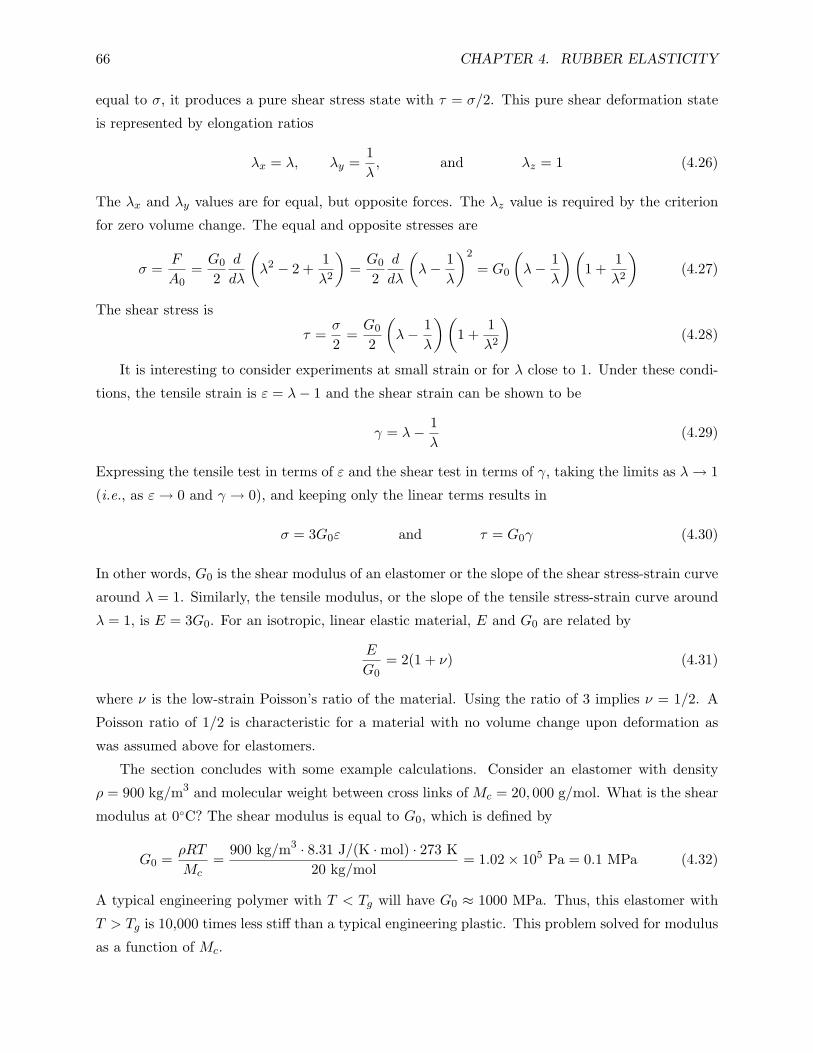
66 CHAPTER 4. RUBBER ELASTICITY
equal to σ, it produces a pure shear stress state with τ = σ/2. This pure shear deformation state
is represented by elongation ratios
λx = λ, λy =1λ, and λz = 1 (4.26)
The λx and λy values are for equal, but opposite forces. The λz value is required by the criterion
for zero volume change. The equal and opposite stresses are
σ =F
A0=G0
2d
dλ
(λ2 − 2 +
1λ2
)=G0
2d
dλ
(λ− 1
λ
)2
= G0
(λ− 1
λ
)(1 +
1λ2
)(4.27)
The shear stress is
τ =σ
2=G0
2
(λ− 1
λ
)(1 +
1λ2
)(4.28)
It is interesting to consider experiments at small strain or for λ close to 1. Under these condi-
tions, the tensile strain is ε = λ− 1 and the shear strain can be shown to be
γ = λ− 1λ
(4.29)
Expressing the tensile test in terms of ε and the shear test in terms of γ, taking the limits as λ→ 1
(i.e., as ε→ 0 and γ → 0), and keeping only the linear terms results in
σ = 3G0ε and τ = G0γ (4.30)
In other words, G0 is the shear modulus of an elastomer or the slope of the shear stress-strain curve
around λ = 1. Similarly, the tensile modulus, or the slope of the tensile stress-strain curve around
λ = 1, is E = 3G0. For an isotropic, linear elastic material, E and G0 are related by
E
G0= 2(1 + ν) (4.31)
where ν is the low-strain Poisson’s ratio of the material. Using the ratio of 3 implies ν = 1/2. A
Poisson ratio of 1/2 is characteristic for a material with no volume change upon deformation as
was assumed above for elastomers.
The section concludes with some example calculations. Consider an elastomer with density
ρ = 900 kg/m3 and molecular weight between cross links of Mc = 20, 000 g/mol. What is the shear
modulus at 0C? The shear modulus is equal to G0, which is defined by
G0 =ρRT
Mc=
900 kg/m3 · 8.31 J/(K ·mol) · 273 K20 kg/mol
= 1.02× 10⁵ Pa = 0.1 MPa (4.32)
A typical engineering polymer with T < Tg will have G0 ≈ 1000 MPa. Thus, this elastomer with
T > Tg is 10,000 times less stiff than a typical engineering plastic. This problem solved for modulus
as a function of Mc.

4.4. MECHANICAL PROPERTIES 67
The previous example can be inverted. In other words, a good way to determine the molecular
weight between cross links is to measure the shear modulus and then use
Mc =ρRT
G0(4.33)
For example, consider a piece of rubber that is 12.7 mm × 1 mm × 40 mm with a shear modulus
of G0 = 2 MPa at 25 C and ρ = 900 kg/m3. What is the molecular weight between cross links?
Substitution gives
Mc =ρRT
G0=
900 kg/m3 · 8.31 J/(K ·mol) · 298 K2× 106 Pa
= 1.114 kg/mol = 1114 g/mol (4.34)
How much work would it take to extend this specimen to λ = 3? By the first law of thermodynamics,
and because internal energy change for an elastomer is zero
∆W = −∆Q = −TV∆S =V G0
2
(λ2 +
2λ− 3)
=508 mm3 · 2 N/mm2
2
(203
)(4.35)
or
∆W = 3.387 J (4.36)
Finally, estimate the temperature rise of the specimen during this experiment (i.e., Gough’s first ex-
periment). Assume the heat capacity of the elastomer is typical for a polymer or Cp = 1.5 J/(g ·K).
The total heat is
∆Q = −∆W = −3.382 J (4.37)
The heat is less than zero since ∆Q is defined as heated added to the sample. For an elastomer
during elongation, the sample heats up and thus the specimen releases heat. This heat will raise
the sample temperature by
∆T = − ∆QmCp
(4.38)
where m is the mass of the specimen:
m = ρV = 0.9 g/cm3 · 508× 10−3 cm3 = 0.4572 g (4.39)
The temperature rise is then
∆T =3.382 J
0.4572 g · 1.5 J/(g ·K)= 4.93C = 8.88F (4.40)
This temperature rise is easily detectable (such as by touching the sample with your lips). In
non-elastomeric materials, the internal energy change is nearly equal to the work and thus heat
during deformation, from the first law of thermodynamics, is
∆Q = ∆U −∆W ≈ 0 (4.41)
In other words, there is no noticeable temperature rise for most materials during elongation.

68 CHAPTER 4. RUBBER ELASTICITY
4.5 Making Elastomers
Many polymers can be made into elastomers. The first step is to find a polymer with T < Tg. If
the selected polymer is not amorphous, the next step is to make it amorphous. The most common
approach to breaking up crystallinity is to copolymerize with a second monomer. If these first two
steps are achieved, the final step is to cross link. The three common strategies to cross linking are:
1. Diene elastomers - if the main polymer chain has double bonds, they can act as reaction sites
to add cross links between chains.
2. Nondiene elastomers - if the main chain does not have any double bonds, cross linking has to
be done by other methods. One common approach is to copolymerize with a small amount
of a monomer having main-chain dienes and cross linking at those diene sites. This approach
might be considered a diene ealstomer, but since most of the network is mostly a nondiene
monomer, they are still called nondiene elastomers.
3. Thermoplastic elastomers - these elastomers do not have chemical cross links. They rely on
physical entanglements to act like cross links. As long as the cross links maintain connection
on the time scale of deformation, they are just as effective as chemical cross links. An
advantage of physical cross links is that the material can be melted and processed by typical
thermoplastic means such as injection molding or extrusion.
4.5.1 Diene Elastomers
A common building block for many commerical diene elastomers is the diene monomer
CH2
R
C CH CH2
When R = H, the monomer is butadiane; when R = CH2, the monomer is isoprene; when R = Cl,
the monomer is chloroprene. When butadiene is polymerized by non-specific methods, it generates
a mixture of three different polymers depending on how the double bond reacts and the location
of the double bond that remains in the polymer:
(CH2 CH)
CH CH2
(CH2
H
HH
C C
HH
CH2)
H
(CH2
H
HH
C C
HH
H
CH2)
Side group cis main chain trans main chain
Each polymer in the mixture has one remaining double bond per repeat unit. The second step in
making butadiene rubber is to use those double bonds to cross link the chains. Although it can

4.5. MAKING ELASTOMERS 69
be done with a mixture of stereochemistries, it is usually preferrable to start with a pure polymer
(e.g., all cis or all trans) by using a stereo-specific polymerization process. A common cross linking
process is sulfur vulcanization invented by Goodyear.2 The process is to heat in the presence of
sulfur and various additives (fatty acids, ZnO2, and accelerators). This step creates Sx linkages
between polymer chains. The process is run until light cross linking is achieved. Too little cross
linking and the product will be too soft. Too much cross linking and it will lose rubber elasticity.
Besides sulfur vulcanization, other methods of cross linking include using peroxides or ionizing
radiation.
Elastomers made with butadiene include butadiene rubber (BR), styrene-butadiene rubber
(SBR), and nitrile rubber (NBR). SBR starts with a copolymer of styrene (10-25%) and butadiene.
The addition of styrene makes the rubber cheaper and improves wear resistance. One application
is for tires. NBR starts with a copolymer of acrylonitrile (15-40%) and butadiene. The addition of
acrylonitrile improves the solvent resistance. One application is for gaskets.
The monomer for natural rubber (NR) is isoprene. Like butadiene, non-specific polymerization
of isoprene results in a mixture of polymers. In contrast, natural rubber from plants is stereospecific.
The all trans version of polyisoprene is known as Hevea rubber. When vulcanized, it is used in
tires. The all cis version is known as Gutta Percha rubber. When vulcanized, it is harder than
Hevea rubber. One application is in covers for golf balls. Unvulcanized natural rubber is crystalline
due to the stereoregular nature of the polymers. The vulcanization breaks up the crystallization
as well as creating the cross links - the two things need to create the low-Tg polyisoprene into an
elastomer. Synthetic versions of natural rubber are possible, but they require use of stereospecific
polymerization methods to start with all trans or all cis polyisoprene polymers.
Rubbers starting with polychloroprene are called Neoprene rubber (CR). These rubbers have
improved solvent resistance. Common applications are for gaskets and O-rings.
4.5.2 Nondiene Elastomers
Numerous polymers based on aliphatic hydrocarbon chains (e.g., polyethylene, polypropylene, etc.)
are inexpensive and have low Tg, but are not elastomeric unless further processed. For example,
polyisobutylene has the repeat unit
( CH2
CH3
C
CH3
)
The main chain has no double bonds and therefore this polymer can not be cross linked by standard
double bond methods. The solution is to copolymerize with a small amount of isoprene. This co-
monomer adds doubles bounds to the main chain which can be reactive sights for cross linking.

70 CHAPTER 4. RUBBER ELASTICITY
Even though cross linking is done with dienes, this rubber is called a non-diene rubber because
most of the main chain lacks double bonds. The resulting elastomer is called Butyl Rubber. It has
lower permeability to oxygen than other elastomers and therefore has application in inner tubes
(e.g., bicycle tires) and weather stripping.
Polyethylene and polypropylene are two of the most widely-produced synthetic polymers. They
are both inexpensive and have Tg’s well below room temperature. Both, however, are highly
crystalline (otherwise they would not be commercially significant polymers due to their low Tg’s).
The first step to using them for elastomers, is to eliminate the crystallinity. This step can be
achieved by an ethylene-polypropylene random copolymer. The random arrangement of monomers
breaks up the regularity needed for crystallization. The next step is to cross link. The copolymer
can be cross linked using peroxides. The resulting elastomer is ethylene-propylene rubber (EPR or
EPM). An alternative is the approach taken with butyl rubber to copolymerize with a third diene
monomer, such as isoprene, and cross link at the added double bond sites. The resulting elastomer
is called ethylene-propylene-diene rubber (EPDM).
If all, or most, of the hydrogens in the above olefinic elastomers are replaced by fluorine (e.g.,
replace ethylene and propylene monomers with tetrafluoroethylene and hexafluoropropylene), the
polymers still have low Tg’s, but have much higher temperature resistance and improved solvent
resistance. When these polymers are lightly cross linked they produce fluoroelastomers. Common
applications are hoses, O-rings, gaskets, tubing, and hydraulics.
Silicone elastomers are made from polymers derived from polysiloxanes with repeat unit
( O
CH3
Si
CH3
)
They have good low-temperature properties, good electrical properties, good resistance to solvents
(e.g., oil), and weather well. Cross linking is done by compolymerizing with silanes that have
functional groups or with peroxides.
4.5.3 Thermoplastic Elastomers
An alternative to chemical cross linking is to prevent flow by physical cross links. Two types of
physical cross links are shown in Fig. 4.6. The top of the figure shows two entangled polymers
being pulled apart. As long as the chains do not break, this arrangement is an effective cross link
that will prevent flow. In real polymers, one does not pull individual molecules, but the result is
similar if the molecular weight is sufficiently high. Given enough time, such entanglements will
unravel allowing flow. On time scales much shorter that this time, the polymer will act like an
elastomer. In fact all amorphous polymers have a region above Tg up to some higher temperature

4.5. MAKING ELASTOMERS 71
Figure 4.6: The top shows two polymer molecules entangles. A short time scales this molecules will notpull apart and the entanglement will act like a cross link. The bottom shows a block copolymer with flexibleblocks and semicrystalline blocks. The semicrystalline blocks can organize to create regions that act likecross links.
with elastomeric properties known at the “rubbery plateau.” The rubbery plateau gets longer
as the molecular weight gets higher. Thus any high molecular weight, amorphous polymer with
Tg below room temperature, will have some elastomeric properties or some temperature and time
range without adding chemical cross links.
The bottom half of Fig. 4.6 shows a different type of physical cross linking and an important
type in the polymer industry. This schematic diagram is for a block copolymer having soft segments
(low Tg amorphous polymer) and hard segments (a semicystalline polymer). When copolymerized
into a block copolymer, the hard segments can segregate in to crystalline regions that act as cross
links for the remaining soft material. It is crucial that the two blocks are from incompatible
polymers such that they segregate into separate regions when solidified. If this polymer is heated
above the melting point of the crystalline region, the cross links will melt and the polymer will flow.
Thus, there elastomers are known as thermoplastic elastomers. When heated then can be molded

72 CHAPTER 4. RUBBER ELASTICITY
or melt spun into fibers. When they cool down, the cross links form again to make an elastomer.
On example is Lycra R© spandex fibers.
Problems
4–1. a. Give three characteristics that a polymer must have for it to have elastomeric properties
at room temperature
b. For each of the characteristics listed in part a, give a physical explanation of why it is
needed for elastomeric properties.
4–2. A rubber consists of a cross-linked network of chains with the molecular weight between cross
links equal to Mc = 15,000 g/mol. The density of the specimen is 0.92 g/cm3.
a. Calculate the shear modulus at 25C.
b. If a cube of this rubber of initial length 10 cm was loaded in uniaxial tension, calculate
the load required to double its length.
c. Give a processing method you could use to increase the shear-modulus of this rubbery
material.
4–3. Polyethylene (PE) is highly crystalline and not elastomeric at room temperature. By copoly-
merizing with two other monomers and further processing it can be converted into an elas-
tomeric product (olefinic rubbers).
a. Describe two co-monomers and the further processing that can be used to convert PE into
olefinic rubber. Explain the reasons for each co-monomer and for the extra processing.
a. If the resulting elastomer is found to have a shear modulus of 100 kPa at 25C and a
density of 0.95 g/cm3, find the molecular weight between cross links and the cross link
density of the polymer.
4–4. Imagine an elastomer subjected to biaxial loading in the x and y directions such that λx =
λy = λ. Find the stress-elongation curve and compare to the result for unaxial loading.

Chapter 5
AMORPHOUS POLYMERS
5.1 Introduction
Polymer solids
5.2 The Glass Transition
Thermo and kinetics of Tg
5.3 Free Volume Theory
Apply to Tg
5.4 Physical Aging
Analysis with free volume theory
73

74 CHAPTER 5. AMORPHOUS POLYMERS

Chapter 6
SEMICRYSTALLINE POLYMERS
6.1 Introduction
Polymer solids
6.2 Degree of Crystallization
Measure and why
6.3 Structures
Unit cell, lamallae, spherulites, etc.
75

76 CHAPTER 6. SEMICRYSTALLINE POLYMERS

Bibliography
1. P. J. Flory. Principles of Polymer Chemistry. Cornell University Press, 1953.
2. C. Goodyear. Vulcanized rubber: Improvements in India-rubber fabrics. US Patent No. 3633,
1844.
3. J. Gough. A description of a property of caoutchouc or Indian rubber. Memoirs of the Literary
and Philosophical Society of Manchester, I:288–295, 1805.
77


