Polyhedral Network Aware Task Scheduling · Network topology abstractions. I. Map task instances to...
32
Polyhedral Network Aware Task Scheduling Martin Kong Brookhaven National Laboratory October 14th, 2017 9th Annual Concurrent Collections Workshop College Station, TX, USA
Transcript of Polyhedral Network Aware Task Scheduling · Network topology abstractions. I. Map task instances to...

Polyhedral Network Aware Task Scheduling
Martin Kong
Brookhaven National Laboratory
October 14th, 20179th Annual Concurrent Collections Workshop
College Station, TX, USA

Introduction: CNCW’17
Introduction
I Context: Shared and distributed memory computers, or any hardwarewhere the underlying network can be modeled
I We introduce different virtual network topologies that allow to modelconcepts such as direction and distance in order to produce a taskschedule
I As an application, we choose the task isolation problem: how toschedule tasks which access shared resources
I Networks and hierarchies are pervasive in computer science, i.e.memory systems, computation graphs, programs
I Concrete instances of this problem are:I False sharingI Placing tasks close or nearby to fixed shared resourcesI Scheduling access of R/W resources (e.g. a file or freshly created data
block)I Job scheduling and accessing a file system (explicit hierarchy) with fast
and slow storage systems
BNL 2

Introduction: CNCW’17
MotivationI Large scale applications require substantial domain, algorithmic and
hardware/software knowledgeI Current and emerging technologies pose an enormous challenge in
terms of performance portability and user productivityI Data movement and long latencies are strong limiting factors for
performanceI Knowledge of the underlying network topology, even in shared-memory
machines, is essential to performance tuningI Diverse background of users calls for abstractions that allow to easily
switch between prescriptive and descriptive programming models andmethods
I New abstractions are necessary in order to exploit and integratenetwork-aware compiler optimizations which:
Avoid communicationPerform efficient communication: minimize synchronization and datamovementSchedule tasks around dataTransfer domain knowledge to the compiler
BNL 3

Introduction: CNCW’17
A Look into the (near) Future
Feature Titan Summit
Application Performance Baseline 5-10x Titan
Number of Nodes 18,688 ~4,600
Node Performance 1.4 TF > 40 TF
Feature 32 GB DDR3 + 6 GB GDDR5 512 GB DDR4 + HBM
NV Memory per Node 0 1600 GB
Total System Memory 710 TB 10 PB DDR4 + HBM + Non-Volatile
System Interconnect (Injection Bandwidth) Gemini (6.4 GB/s) Dual Rail EDR-IB (23 GB/s)
Interconnect Topology 3D Torus Non-blocking Fat Tree
Procesor 1 AMD Opteron + 1 NVIDIA Kepler 2 IBM Power9 + 6 NVIDIA Volta
File System 32 PB, 1 TB/s, Lustre 250 PB, 2.5 TB/s GPFS
Peak Power 9 MW 15 MW
BNL 4

Introduction: CNCW’17
Context
I Previously considered data dependences and “performancedependences” (e.g. additional dependences that affect scheduling,directly or indirectly)
I We leverage polyhedral tools to model different network topologiesI Goal: composability of networksI Polyhedral compilation frameworks leverage lexicographic minimizationI Optimization of Manhattan-distance type problems are not immediately
modelableI In this work, we provide abstractions for modeling different types of
network topologiesI We follow an iterative optimization process
BNL 5

Introduction: CNCW’17
Contributions
- (Macro-) Dataflow Programming
- Dynamic Single Assignment
- (Manual) Tuners- Shared + Distributed
CnC1
1 Budimlic et. al, “Concurrent Collections”, Scientific Programming, 20102 A. Sbirlea, L.-N Pouchet and V. Sarkar, “DFGR: an intermediate graph representation formacro-dataflow programs”, DFM, 2014
Kong, Pouchet, Sadayappan, Sarkar, “PIPES: A Language and Compiler for Task-Based
Programming on Distributed-Memory Clusters”, SC, 2016BNL 6

Introduction: CNCW’17
Contributions
- (Macro-) Dataflow Programming
- Dynamic Single Assignment
- (Manual) Tuners- Shared + Distributed
- Slight variation of CnC
- Recognition of Polyhedral subsets,Automatic coarsening
- Hierarchy of conceptsfor sets
CnC1
DFGL2
1 Budimlic et. al, “Concurrent Collections”, Scientific Programming, 20102 A. Sbirlea, L.-N Pouchet and V. Sarkar, “DFGR: an intermediate graph representation formacro-dataflow programs”, DFM, 2014
Kong, Pouchet, Sadayappan, Sarkar, “PIPES: A Language and Compiler for Task-Based
Programming on Distributed-Memory Clusters”, SC, 2016BNL 6

Introduction: CNCW’17
Contributions
DFGL2
PIPES
CnC1- (Macro-) Dataflow
Programming- Dynamic Single
Assignment- (Manual) Tuners- Shared + Distributed
- Slight variation of CnC
- Recognition of Polyhedral subsets,Automatic coarsening
- Hierarchy of conceptsfor sets
- Compiler support for “graph” transformations (e.g., coarsening, coalescing)
- Language constructs for task/data placement, and communications
- Automatic generationof Intel CnC C++ tuners
- Network aware task scheduling
- Isolate relations
1 Budimlic et. al, “Concurrent Collections”, Scientific Programming, 20102 A. Sbirlea, L.-N Pouchet and V. Sarkar, “DFGR: an intermediate graph representation formacro-dataflow programs”, DFM, 2014
Kong, Pouchet, Sadayappan, Sarkar, “PIPES: A Language and Compiler for Task-Based
Programming on Distributed-Memory Clusters”, SC, 2016BNL 6

Background: CNCW’17
PIPES Language Features
I Language features aretask-centric
I Virtual topologies
I Task placement
I Data placement
I Data communication (pull or pushcommunication model)
BNL 7

Background: CNCW’17
MatMul in PIPES
1 Parameter N, P;2 // Define data collections3 [float* A:1..N,1..N];4 [float* B:1..N,1..N];5 [float* C:1..N,1..N,1..N+1];6 // Task prescriptions7 env :: (MM:1..N,1..N,1..N);8 // Input/Output:9 env -> [A:1..N,1..N];
10 env -> [B:1..N,1..N];11 env -> [C:1..N,1..N,1];12 [C:1..N,1..N,N+1] -> env;13 // Task dataflow14 [A:i,k],[B:k,j],[C:i,j,k] -> (MM:i,j,k) -> [C:i,j,k+1];
Figure: PIPES Matrix Multiplication
BNL 8
Background: CNCW’17
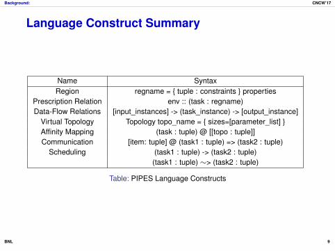
Language Construct Summary
Name SyntaxRegion regname = { tuple : constraints } properties
Prescription Relation env :: (task : regname)Data-Flow Relations [input_instances] -> (task_instance) -> [output_instance]
Virtual Topology Topology topo_name = { sizes=[parameter_list] }Affinity Mapping (task : tuple) @ [[topo : tuple]]Communication [item: tuple] @ (task1 : tuple) => (task2 : tuple)
Scheduling (task1 : tuple) -> (task2 : tuple)(task1 : tuple) ∼> (task2 : tuple)
Table: PIPES Language Constructs
BNL 9

Background: CNCW’17
Virtual Topologies and Task MappingI Virtual topologies (VTs)
represent the logical underlyingcomputer grid/cluster
I Each element in the set is aprocessor
I Requires a logical-to-physicalmapping
1 // 2D topology, no more than 256x256 processors
2 Parameter P : 1..256;3 Topology Topo2D = {4 sizes=[P,P];5 cores=[i,j] : { 0 <= i < P, 0
<= j < P};6 };
BNL 10

Background: CNCW’17
Virtual Topologies and Task MappingI Mappings of tasks to elements in
the topology
I Task (instance) will execute onthe processor it is mapped to
I Always enforced by run-time
I Requires the topology to bedefined
I Maps directly to the compute_ontuner
1 (task:tag-set) @ Topo2d(point);
BNL 10

Compiler: CNCW’17
Overall Approach
I Network topology abstractionsI Map task instances to virtual topology via Affinity Tasks Mappings (ATM)I Introduce isolate relations and isolate dependencesI Compute in closed for the possible task interleavingsI Filter / prune unwanted tasks orderings from the closed formI For each point in the closed form, iteratively compute its costI Apply lexicographic minimization to determine the best execution order
BNL 11

Compiler: CNCW’17
Network Topologies
I PIPES uses an abstraction that allow to pin task instances to processingelements / cores; main purpose is to determine if tasks execute on thesame location; then generate Intel CnC++ tuners
I In this work: Implemented two different topologies: mesh and fat tree
I Pending to implement: torus / meshes + wraparound, hypercubes,hierarchies
I Each network type requires different set of abstractions
I Abstractions allow modeling concepts such as dimension, distance ordirection
I In the future, want to pursue composing two or more topology types, soas to faithfully represent upcoming HPC and Data Analytics clusters
BNL 12

Compiler: CNCW’17
Driving Example
I Consider a 4x4 mesh and 4 tasks(A,B,C,D)
I What if A has to start thecomputation?
I What if any task can start thecomputation?
I What if wrap-around communicationis allowed?
I In general, avoiding ping-pong-ingaround
A C
D
B
A C
D
B
A C
D
B
A C
D
B
A C
D
B
BNL 13

Compiler: CNCW’17
Network Topologies: N-dimensional MeshesKey: idea: translate task tuple to network coordinates,then compute distance between network coordinates.Example:
1 Compute task topology coordinates:A=G[0,0]; B=G[3,3];C=G[0,3]; D=G[1,0]
2 Compute task-to-task topology directions:Dir(A,B) = [3,3]; Dir(B,C) = [0,-3];Dir(C,D) = [-3,1]
3 Compute “positive directions”:+Dir(Dir(A,B)) = [3,3];+Dir(Dir(B,C)) = [0,3];+Dir(Dir(C,D)) = [3,1];
4 Compute task-to-task topology distance:Dist(A,B) = MultiplexAddMap([3,3]) = 6Dist(B,C) = MultiplexAddMap([0,3]) = 3Dist(C,D) = MultiplexAddMap([3,1]) = 4
A C
D
B
BNL 14

Compiler: CNCW’17
Network Topologies: Fat TreesI Distance metrics in fat tree type
of network are non-linearI Coordinate space is one
dimensionalI Task tuples must be “flattened” to
represent processors in the gridI Restricted to fixed
(non-parametric) network sizesI Approach: explicitly construct a
distance map from a pair ofprocessors to a fixednon-parameteric value, i.e.[[Pi]−> [Pj]]−> [distance]
I Does not require the coordinateto direction map nor thepositive direction map
I Observe the recursive nature
0P0P1P2P3P4P5P6P7
P0 P1 P2 P3 P4 P5 P6 P7
1 2 2
2 2
4 4 4 4
4 4 4 4
4 4 4 4
4 4 4 4
4 4 4 4
4 4 4 4
4 4 4 4
4 4 4 4
2 2
2 2
2 2
2 2
2 2
2 2
0 0
0 0
0 0
0
1
1 1
1 1
1 1
BNL 15

Compiler: CNCW’17
Network Topology Abstractions
I Affinity maps (task tuple to network coordinate maps)
I Coordinate to direction maps (each dimension can be +/-)
I Direction unification map: consider different routes along eachdimension and direction (several disjunctions), e.g. in meshes withwraparound
I Direction to distance maps: make directions positive
I Cummulative distance maps: “Multiplex Add Map”
BNL 16

Compiler: CNCW’17
Building the Closed Form of the ExplorationSpace
I Compact and closed form for encoding task orderings at the coarse levelI Assign to each task a fixed integerI Start with the TT potential task orderings (T : number of lexical tasks),
fixed and known at compile timeI The exploration space consist of the set of points in a T-dimensional
tuple space.I Add bounding constraints:~t = (t1, t2, ..., tT), ∀ ti ∈ [1..T]I Add constraints to remove meaningless points, e.g. (1,1,1) which
represents the same task being executed: ∑ ti = T× (T +1)/2I Add constraints to enforce data dependences, i.e. if task 1 is a
dependence of task 2 then: ti = 1 and tj = 2, for some j > iI Each point in the set represents a full execution path (e.g.
3→ 1→ 4→ 2)
BNL 17

Compiler: CNCW’17
Pruning the Scheduling SpaceWe consider three types of pruning constraints that are added to thecomplete space, e.g. (t1, t2, ..., tT), ti ∈ [1..T]
I Data dependence edges: “A(1) must to execute before B(2)”
I Scheduling edges (for performance): “We want A(1) to execute beforeB(2)”
I Isolation edges: “We want either A(1) before B(2) or B(2) before A(1)”
Several disjunctions might be required to model the constraints, in particularfor the isolation edges
A few more considerations:
I In theory, we could still have meaningless points, e.g. (1,1,4,4) = 10I In practice, these would be mostly naturally pruned by the above
constraintsI To be safe, we do a manual check before the next stage to guarantee
that all entries in a vector are distinctBNL 18

Compiler: CNCW’17
Iteratively Computing Path Costs1: space← compute_closed_form (T,program)2: for each~t = (t1, t2, ..., tN) ∈ space do3: path(~t)← 04: for each (ti, ti+1) ∈ (t1, t2, ..., tN) do5: Fetch task domains T(ti) and (Ti+1)6: Fetch task affinity maps: AM(ti) and AM(Ti+1)7: Build synchronization map: sync_map← T(ti)→ T(ti+1)8: Intersect dependences T(ti)⇒ T(ti+1) with sync_map9: Compute processor synchronization map (PSM): PSM
← AM(ti)−1 ◦ sync◦AM(Ti+1)10: Compute “processor coordinate difference” (PCD) with ISL
deltas_map (PSM)11: Apply network specific coordinate-to-distance map to PCD12: edge(i)← quasi_polynomial_sum(PSM)13: path(~t)← path(~t) + edge(i)14: end for15: M← M ∪ path(~t)16: end for17: result← lexmin(M)
BNL 19
Compiler: CNCW’17
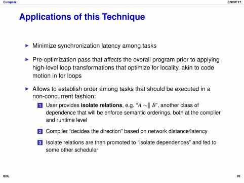
Applications of this Technique
I Minimize synchronization latency among tasks
I Pre-optimization pass that affects the overall program prior to applyinghigh-level loop transformations that optimize for locality, akin to codemotion in for loops
I Allows to establish order among tasks that should be executed in anon-concurrent fashion:
1 User provides isolate relations, e.g. “A∼‖ B”, another class ofdependence that will be enforce semantic orderings, both at the compilerand runtime level
2 Compiler “decides the direction” based on network distance/latency
3 Isolate relations are then promoted to “isolate dependences” and fed tosome other scheduler
BNL 20

Compiler: CNCW’17
Applications of this Technique
I This technique has the potential to reduce the runtime schedulingoverhead by substantially narrowing down the scheduling options
I Autotuning: coupled with auto-generated task mappings, allows todetermine suitable mappings and task schedules
I Applicable to several task parallel and data-flow runtimes (CnC!!)
BNL 21

Compiler: CNCW’17
Restrictions of the Approach
I Very computational expensive, even in non-parametric cases
I Limited to ∼ 10 tasks (millions of possible interleavings) and taking ∼ 10min
I Disallow edges that induce loops in the graph
I Some networks cannot be modeled with affine parametrics constraints,resort to use large fixed values and bound network parameters by thecontext
BNL 22
Results: CNCW’17
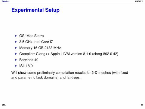
Experimental Setup
I OS: Mac SierraI 3.5 GHz Intel Core i7I Memory:16 GB 2133 MHzI Compiler: Clang++ Apple LLVM version 8.1.0 (clang-802.0.42)I Barvinok 40I ISL 18.0
Will show some preliminary compilation results for 2-D meshes (with fixedand parametric task domains) and fat-trees.
BNL 23
Results: CNCW’17
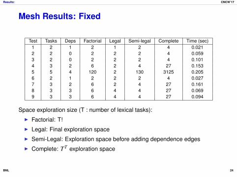
Mesh Results: Fixed
Test Tasks Deps Factorial Legal Semi-legal Complete Time (sec)1 2 1 2 1 2 4 0.0212 2 0 2 2 2 4 0.0593 2 0 2 2 2 4 0.1014 3 2 6 2 4 27 0.1535 5 4 120 2 130 3125 0.2056 2 1 2 2 2 4 0.0277 3 2 6 2 4 27 0.1618 3 3 6 4 4 27 0.0699 3 3 6 4 4 27 0.094
Space exploration size (T : number of lexical tasks):I Factorial: T!I Legal: Final exploration spaceI Semi-Legal: Exploration space before adding dependence edgesI Complete: TT exploration space
BNL 24

Results: CNCW’17
Mesh Results: Parametric
Test Tasks Deps Factorial Legal Semi-legal Complete Time (sec)01 2 0 2 2 2 4 0.05602 3 2 6 2 7 2703 3 1 6 3 7 27 0.03704 4 1 24 17 44 256 0.105 5 1 120 120 381 3,12506 5 4 120 4 381 3,12507 6 5 720 12 4,332 46,656 0.1508 7 5 5,040 84 60,691 823,543 0.9609 9 7 362,880 648 19,610,233 387,420,489 23310 9 8 362,880 1 19,610,233 387,420,489 28.811 10 9 3.63E+06 2 432457640 10,000,000,000 317.2
Space exploration size (T : number of lexical tasks):I Factorial: T!I Legal: Final exploration spaceI Semi-Legal: Exploration space before adding dependence edgesI Complete: TT exploration space
BNL 25

Results: CNCW’17
Fat Tree Results
Test Fat Tree Tasks Deps Factorial Legal Semi-legal Complete TimeMax Size (min + sec)
1 16 2 1 2 2 2 4 0m0.077s2 32 2 1 2 2 2 4 0m0.167s3 64 2 1 2 2 2 4 0m0.495s4 128 2 1 2 2 2 4 0m1.583s5 256 2 1 2 2 2 4 0m5.556s6 512 2 1 2 2 2 4 0m21.163s7 1024 2 1 2 2 2 4 1m21.719s8 2048 2 1 2 2 2 4 5m31.795s9 256 5 3 120 12 130 3125 2m5.986s10 256 5 4 120 34 130 3125 5m58.886s11 256 5 6 120 130 130 3125 22m57.720s
Space exploration size (T : number of lexical tasks):I Factorial: T!I Legal: Final exploration spaceI Semi-Legal: Exploration space before adding dependence edgesI Complete: TT exploration space
BNL 26

Conclusion: CNCW’17
Future WorkI Complete implementation of torus networks, hypercubes and explicit
hierarchiesI Enable composability of network topology abstractionsI Integrate resource features into topology abstraction:
To model super nodes that have access near to accelerators or tomemory nodesSpecialized resource types e.g. streaming nodes, compute intensivenodes, memory nodes, storage nodes, etc
I Potential direction: focus on file access scheduling (e.g. in HPF5) byusing the data file and block structure to construct the program graph
I Complete integration to PIPES compilerI Leverage the newly introduced constructs to efficiently implement and
perform communication patterns such as:All to all communicationMulticast and broadcastNearest neighbor type of communication
I Improve the scalability of the technique: Perform cuts on the graph,search for “bridge tasks” and “articulation tasks”
BNL 27

Conclusion: CNCW’17
Das Ende
Thanks for listening
Questions?
BNL 28


![Adaptive Affinity Fields for Semantic Segmentationstellayu/publication/doc/2018aafECCV.pdfAdaptive Affinity Fields for Semantic Segmentation Tsung-Wei Ke* [00000003 1315 3834], Jyh-Jing](https://static.fdocuments.net/doc/165x107/600d21f124b11f24f414f7c9/adaptive-afinity-fields-for-semantic-segmentation-stellayupublicationdoc2018aafeccvpdf.jpg)