1

Pollution Exposure, Child Health and Latent Factors:

Evidence for Germany

Katja Coneus

SAP Walldorf Email: KaConeus@web.de

C. Katharina Spiess

(corresponding author)

German Institute for Economic Research (DIW Berlin), and Free University Berlin

DIW Berlin Mohrenstrasse 58

10117 Berlin Germany

Email: kspiess@diw.de Tel: +49 30 89789-254 Fax: +49 30 89789-109

December 2011

2

Abstract:

This paper examines the impact of outdoor pollution and parental smoking on children’s health

from birth until the age of three years in Germany. We use representative data from the German

Socio-Economic Panel (SOEP), combined with five air pollution levels. These data were provided

by the Federal Environment Agency and cover the years 2002 to 2007. Our work makes two im-

portant contributions. First, we use European data to replicate and extend an important US study by

following the effects of pollution exposure and parental smoking on child health during the first

four years of life. For infants, as well as for two- to three-year-olds, we are able to account for

time-invariant and unobserved neighborhood and maternal characteristics. Second, instead of rely-

ing solely on mean pollution levels, we also calculate latent pollution measures. Our results suggest

a significantly negative impact of some pollutants on infant health. High exposure to CO prior to

birth causes, on average, a 289 gram lower birth weight. With respect to toddler health, we find that

disorders such as bronchitis and respiratory illnesses are affected particularly by O3 levels.

JEL: I12, Q53, J13 Keywords: pollution exposure, latent factors, child health, early childhood �

Acknowledgement: This paper profited substantially from the support of Tobia Lakes and Maria Brückner from the Geomatics Department at the Institute of Geography, Humboldt University Berlin. We also thank Janet Currie and Johannes Schmieder for their invaluable comments during a research stay at Co-lumbia University in 2009. Moreover, we thank the editor and anonymous referees for very helpful comments. Elisabeth Bügelmayer and Eric Dubiel provided invaluable research assistance.

3

1 Introduction

Almost all Western industrialized countries have introduced measures for pollution abatement.

These measures are often justified as promoting human health. Although there is still much to learn

about pollution and the mechanisms underlying it, past research has argued that its impacts on adult

health tend to be long-term and those on child health more short-term. To examine whether this

latter assumption holds true, we study the effect of air pollution exposure on child health. The con-

nection between them is of crucial interest due to children’s high sensitivity to pollution. In chil-

dren, the rate of metabolism is higher than in adults, which means that children need, relatively

speaking, more energy and oxygen. Children also take in more food per kilogram of body weight

and therefore more pollutants. Furthermore, they breathe more per kilogram of body weight, which

means that the respiratory tract is more stressed by pollutants. Moreover, whereas adults may expe-

rience the onset of disease long after they were first exposed to pollutants, the connection between

cause and effect is much closer temporally in children: in the case of infant death, it is immediate.

In addition, there is increasing evidence of long-term effects of poor infant health on later health

outcomes (Currie 2009; for more recent overview, see Currie 2011).

The economic literature has produced a number of studies focusing on air pollution and child

health in the United States (see Section 2). However, there is little evidence from other industrial-

ized countries on different measures of pollution abatement.1 The German Federal Environment

Agency (“Bundesumweltamt”) is responsible for pollution measurement. Germany is covered by a

network of stations that regularly measure pollution levels. Yet these data have seldom been used

to analyze the relationship between pollution and child health. One exception is the German Envi-

ronmental Survey for Children. In this survey, which is part of a larger study of child health in

Germany (Kurth et al. 2008), a special module was added from 2003 to 2006 to measure the influ-

ence of environmental factors on child health. Exposure to chemical pollutants, mold spores, and

noise was examined in a representative sample of 1,790 children between the ages of 3 and 14.

With respect to one aspect of CO indoor pollution intensity, the survey shows that around 50% of

the children were living in households with at least one smoker. However, the earlier years of life

were not taken into account in this study. For a study focusing on earlier years in the German con-

text, see Lüchinger (2009), who combined data from the Federal Environment Agency with data

from birth statistics. However, given the data used, it was not possible to control for a broader set

1 There are other studies focusing on environmental issues in developing countries. For example, see the study by Kim (2009) who analyzed the impact of rainfall on child health in the first five years of a child’s life, also addressing the issue of child mortality.

4

of child and family characteristics. This was a limitation we have been able to overcome in the pre-

sent study through the use of representative survey data.

In this study, we use data from the German Socio-Economic Panel (SOEP) combined with data

from the German Federal Environment Agency. We make two important contributions to the litera-

ture. First, we take a similar approach to Currie et al. (2009), but expand the perspective from the

US (New Jersey) to a European context. To enable comparison, we use similar health and pollution

data from Germany. In contrast to Currie et al. (2009), we are able to follow the effects of pollution

exposure on child health across the first four years of life. We observe infant health outcomes in the

first year of life as well as health outcomes at the ages of two to three years. For infants as well as

for two- to three-year-olds, we are able to account for time-invariant and unobserved neighborhood

and mother-specific characteristics, which is in line with the methodology used by Currie et al.

(2009). Second, we calculate different pollution intensity measures. Instead of relying solely on

mean pollution levels, we also quantify latent pollution exposure. This allows us to summarize all

pollution values into few meaningful values.

2 Background

Several past studies using US data have examined the link between air pollution and infant health.

Not all of them focus on causal relationships. Yet the question of causality is of key importance,

especially because many of the studies investigating the link between pollution and health have

neglected to consider the possibility that pollution exposure is endogenously determined—for ex-

ample, when individuals make choices to maximize their wellbeing and move to cleaner environ-

ments. Parents with high preferences for less polluted air are more likely to move to areas with bet-

ter air quality and are also more likely to invest more in their child’s health. Failing to appropriately

account for such actions can yield misleading estimates of the causal effect of pollution on health.

This has to be taken into consideration when summarizing the relevant studies.

Chay and Greenstone (2003) use historic data to analyze the implementation of the Clean Air Act of

1970 and the recession of the early 1980s. They take the 1981 to 1982 recession as a “quasi-

experiment” to estimate the impact of total suspended particulates (TSPs) on infant mortality. They

find that an one percent reduction in TSPs results in a 0.35 percent decline in the infant mortality

rate at the county level, implying that 2,500 fewer infants died from 1980–1982 than would have

died in the absence of the TSP reductions. Their estimates are stable across a variety of specifica-

tions.

5

Neidell (2004) and Currie and Neidell (2005), using data from California, address the endogeneity

issue by assessing the within zip code variation in pollution levels rather than by exploiting quasi-

natural experiments. They focus on infant health, including birth weight, gestational age, infant

mortality, and asthma. Neidell (2004) estimates the effect of air pollution on child hospitalizations

for asthma using naturally occurring seasonal variations in pollution within zip codes. He reports

that the effect of pollution is greater for children of lower socio-economic status (SES), indicating

that pollution is one potential mechanism by which SES affects health. However, all of these stud-

ies find mixed results on the effects of pollution on health at birth.

The study by Currie et al. (2009) for New Jersey makes two improvements on the two studies men-

tioned above. First, they determine the closest measuring stations to the households using the exact

coordinates of the household address instead of the coordinates of the zip code center. Second, in

addition to accounting for unobservable heterogeneity of the neighborhood, they also control for

unobserved characteristics of the mother. The results confirm that CO has a significant effect on

fetal health, birth weight, and infant mortality, even at low levels of pollution. The results are ro-

bust against different specifications. A recent study by Lleras-Muney (2010) based on data on US

military families uses changes in location due to military personnel transfers (which are not matters

of individual choice) to identify the causal impact of pollution on children’s respiratory hospitaliza-

tion. The study is unique in that it covers children from birth to the age of five. The results suggest

that only ozone has an adverse effect on the health of military children, although not among infants.

A recent paper by Currie and Walker (2011) analyzes the effects of the introduction of electronic toll

collection in two US states on infant health measures such as premature birth and low birth weight.

They report that electronic toll collection reduced prematurity and low birth weight among mothers

within two kilometers of a toll plaza by 10.8 percent and 11.8 percent, respectively, relative to

mothers within two and ten kilometers of a toll plaza. There were no immediate changes in the

characteristics of mothers or in housing prices near toll plazas that could explain these changes.

The results are robust to many changes in specification and suggest that traffic congestion contrib-

utes significantly to poor health among infants. Another study by Currie et al. (2011) on the effect

of site cleanups on infant health provides a relevant example of how policy measures affecting the

quality of the immediate environment in turn affect infant health.

6

The only study to date on Germany is that of Lüchinger (2009) mentioned above. The study esti-

mates the effect of sulfur dioxide pollution on infant mortality in Germany from 1985 to 2003. To

avoid simultaneity problems, the author exploits the natural experiment created by the mandated

desulfurization at power plants, with wind directions dividing counties into treatment and control

groups. He found that the observed reduction in pollution implies an annual gain of 850 to 1,600

infant lives. Estimates are robust to controls for economic activity, climate, reunification effects,

rural/urban trends, and total suspended particulate pollution and are comparable across subsamples.

In our study, we control for unobservable time-invariant characteristics of the neighborhood and

the mother in line with the study by Currie et al. (2009). But contrary to Currie et al. (2009), we

employ five different air pollution values, carbon monoxide (CO), ozone (O3), particulate matter

(PM10), nitrogen dioxide (NO2), and sulfur dioxide (SO2). For a short summary of how these pollu-

tants could affect child health, see Appendix AI.

Given this rich set of pollution measures, it is questionable which value is the most appropriate to

measure health effects. In the literature, it is not clear which pollution value is suitable for describ-

ing outliers or the duration of exposure in an appropriate manner. For instance, the study by Currie

et al. (2009) finds that the exposure in the last trimester of pregnancy influences birth outcomes

significantly negatively, at least for CO, but not in the first or second trimesters. However, the re-

sults indicate the multicollinearity of the three mean values (see also algebraic signs in Section 4).

Therefore, the problem is how to make use of the variety of measurement values2 in such a way

that no important information is lost by aggregating the measurement values, and at the same time

to ensure that the variety of (mean) values does not lead to multicollinearity in the results. For this

reason, besides different mean value combinations, we also use latent factors that compress the

variety of information into useful values.

3 Data

The main data source used in this study is the German Socio-Economic Panel (SOEP). It is a repre-

sentative national longitudinal data set for Germany that annually surveys households and all

household members aged 16 and above. The SOEP started in 1984 (Wagner et al. 2007).3 It pro-

vides an informative database with a rich set of indicators of both parents’ and children’s character-

istics. Since 2003, the SOEP has collected detailed information on child health through an addi-

tional questionnaire given to mothers of very young children. For our analysis, we use data on the 2 The yearly mean pollution value consists of 17,520 = (2x24x365) single half-hourly pollution values. 3 See http://www.diw.de/soep for more information on the SOEP.

7

2002 to 2007 birth cohorts. The SOEP sample design enables us to distinguish children in their first

year of life (infants) from children at two to three years of age (toddlers). The sample size for the

newborns varies between 1,154 and 1,268, and for the two- to three-year-olds between 629 and

775. The information provided in the SOEP allows us to use the following health measures: weight

and length at birth, fetal growth, and any disorders a child develops later (e.g., motor or visual im-

pairments).

In the SOEP data, the child characteristics can be linked with maternal and family characteristics.

Here, we observe maternal age, education, and family characteristics. Moreover, we match the pa-

ternal information and household-related characteristics (household net income, municipality size,

and migration background) to child-related variables.4 The data also allow us to identify siblings

born within a household.

The SOEP data furthermore provide information on the smoking behavior of both parents. We use

this as an approximation for CO exposure within the household. However, there are also other

sources of indoor air pollution, including pollution from various combustion sources, building ma-

terials and furnishings, and products for household cleaning and maintenance. This should be taken

into account in the interpretation of our results.

For our analysis, we link the SOEP data with data from the Federal Environment Agency by

matching SOEP households with the pollutant measures from the nearest measuring station. Since

we know the exact coordinates of these measuring stations as well as the exact coordinates of the

center of the zip code area for each SOEP household, it was possible to identify the nearest station

(short distance principle) for each year5 and each household. The distance between the station and

the household is often less than a kilometer. In urban areas, the mean distance between the house-

hold and the monitor is less than 3 kilometers. In rural areas, the maximum distance between the

household and the measuring station is 30 kilometers. However, we make use of the fact that pollu-

tion levels in rural areas do not change as much over large distances as they do in urban areas. The

regional distribution of the SOEP households and the measuring stations is presented in Fig. A1,

Appendix.6

4 This is a dummy variable, which takes the value 1 if the mother or father or both parents have an immigration back-ground and 0 otherwise. 5 This approach, which we had to use for data security reasons, is not as precise as using the exact “household coordi-nates.” 6 Since not all the measuring stations in Germany measure all five air pollutants, there are households that have to be assigned to two measuring stations.

8

The detailed data on air pollution levels cover the years 2002 to 2007. The data are measured at

monitors. In Germany, each state has between 11 (Bremen) and 268 (North Rhine-Westphalia)

monitors. Altogether, 1,305 monitors in the 11 states measure air quality in Germany. The Federal

Environment Agency compiles the measurements in a data base and provides information on pollu-

tion in Germany, broken down by pollutant source. Most of the measuring stations do not measure

all five of the pollutants used in our analysis. In many cases, CO, NO2, and PM10 are measured at

the same station, especially in traffic zones.7 Which stations measure which pollutants depends

significantly on the location and the specific problems affecting it. For instance, sites with high

traffic are equipped with devices measuring the pollutants typical of this area only, such as PM10,

NO2, and CO. On the other hand, O3 is not a problem in traffic zones, but it is in urban, suburban,

and rural areas. For CO, NO2, SO2, and O3, half-hourly values are measured for every station and

every day, and hourly values for PM10. In our analysis, we use monthly means for the individual

pollutants, which are all calculated according to the guidelines for calculating and analyzing emis-

sion data on the basis of the official EU guidelines.8 Mean values for a week, decade, month, and

year are measured on the basis of (half-)hourly means. The EoI (Exchange of Information) guide-

lines stipulate that hourly means may only be calculated when 75 percent of the data is available,

that is, when both half-hourly means are provided. Based on the hourly means, daily means may

only be calculated when at least 13 hourly means are available and when, at the same time, no more

than six successive hourly means are missing.

The calculated average seasonal variation for the five pollutants for the years 2002 to 2007 can be

seen in Fig. 1. The figure shows that for each air pollutant, considerable variation is observable not

only within months but also over years.

Fig. 1: Seasonal variation in air pollution (2002-2007)

7 Detailed information on which stations in Germany measure which pollutants can be found at http://www.env-it.de/stationen/public/open.do (accessed August 10, 2010). 8 See Council Decision of 27 January 1997 establishing a reciprocal exchange of information and data from networks and individual stations measuring ambient air pollution within the Member States (97/101/EC) (short term: Exchange on Information decision on Air - EoI on Air) and changes made by the Council on 17 October 2011 (2001/752/EC).

9

.3.4

.5.6

.7C

O

2002 2004 2006

34

56

7SO

2

Jan 2002 Jan 2006Jan 2004

2025

3035

NO

2

Jan 2002 Jan 2004 Jan 2006

2030

4050

6070

O3

Jan 2002 Jan 2004 Jan 2006

2025

3035

PM10

Jan 2002 Jan 2004 Jan 2006

Source: Federal Environment Agency (2002-2007): own calculations.

Having detailed data on pollution levels collected at different points in time could theoretically

offer advantages. However, as has been shown by Kvedaras and Rackauskas (2010), variables of

different frequencies can cause a problem. In some cases, standard aggregation no longer works.

This argument has been widely ignored in the previous literature. We argue that the method of data

orthogonalization described above provides a possible means of dealing with this. For more details

see section 4.

With respect to child health, our data set offers various options. Finding the appropriate measure of

child health status is a challenge (see also Case et al. 2002). Health has many dimensions, including

mental and physical health, chronic conditions, environmental conditions, nutrition, and injuries.

Studies on Western industrialized countries often use low birth weight (LBW) as an indicator of

poor health at birth (e.g., Oreopoulos et al., 2008). Alternative measures of child health are bed

days and hospitalization episodes. Until a global definition of child health is found, we argue that it

is useful to employ a variety of measures as they become available. This is a crucial advantage of

the data used here: the SOEP allows us to observe different types of child health measures (for oth-

er SOEP-based studies using similar child health measures, see, e.g., Dunkelberg and Spiess, 2009;

Cawley and Spiess, 2008; and Coneus and Spiess, 2011). For all age cohorts, we used anthropo-

metric (health) measures such as weight and length of the child at birth. Anthropometric health

10

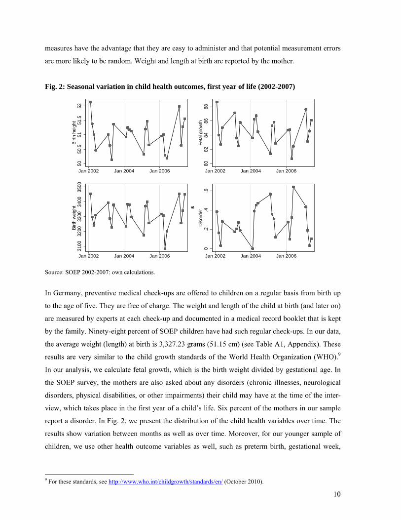
measures have the advantage that they are easy to administer and that potential measurement errors

are more likely to be random. Weight and length at birth are reported by the mother.

Fig. 2: Seasonal variation in child health outcomes, first year of life (2002-2007) 50

50.5

5151

.552

Birt

h he

ight

Jan 2002 Jan 2006Jan 2004

8082

8486

88Fe

tal g

row

th

Jan 2002 Jan 2006Jan 2004

3100

3200

3300

3400

3500

Birt

h w

eigh

t

Jan 2002 Jan 2004 Jan 2006

0.2

.4.6

Dis

orde

r

Jan 2002 Jan 2006Jan 2004

Source: SOEP 2002-2007: own calculations.

In Germany, preventive medical check-ups are offered to children on a regular basis from birth up

to the age of five. They are free of charge. The weight and length of the child at birth (and later on)

are measured by experts at each check-up and documented in a medical record booklet that is kept

by the family. Ninety-eight percent of SOEP children have had such regular check-ups. In our data,

the average weight (length) at birth is 3,327.23 grams (51.15 cm) (see Table A1, Appendix). These

results are very similar to the child growth standards of the World Health Organization (WHO).9

In our analysis, we calculate fetal growth, which is the birth weight divided by gestational age. In

the SOEP survey, the mothers are also asked about any disorders (chronic illnesses, neurological

disorders, physical disabilities, or other impairments) their child may have at the time of the inter-

view, which takes place in the first year of a child’s life. Six percent of the mothers in our sample

report a disorder. In Fig. 2, we present the distribution of the child health variables over time. The

results show variation between months as well as over time. Moreover, for our younger sample of

children, we use other health outcome variables as well, such as preterm birth, gestational week,

9 For these standards, see http://www.who.int/childgrowth/standards/en/ (October 2010).

s

11

head circumference, and LBW. However, we do not find any significant results for the health

measures and thus do not discuss or use them further.

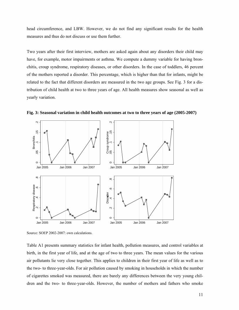
Two years after their first interview, mothers are asked again about any disorders their child may

have, for example, motor impairments or asthma. We compute a dummy variable for having bron-

chitis, croup syndrome, respiratory diseases, or other disorders. In the case of toddlers, 46 percent

of the mothers reported a disorder. This percentage, which is higher than that for infants, might be

related to the fact that different disorders are measured in the two age groups. See Fig. 3 for a dis-

tribution of child health at two to three years of age. All health measures show seasonal as well as

yearly variation.

Fig. 3: Seasonal variation in child health outcomes at two to three years of age (2005-2007)

0.0

5.1

.15

.2B

ronch

itis

Jan 2005 Jan 2006 Jan 2007

0.0

5.1

.15

.2C

roup s

yndro

me

Jan 2005 Jan 2006 Jan 2007

0.2

.4.6

.8R

esp

irato

ry d

isease

Jan 2005 Jan 2006 Jan 2007

0.2

.4.6

.8D

isord

er

Jan 2005 Jan 2006 Jan 2007

Source: SOEP 2002-2007: own calculations.

Table A1 presents summary statistics for infant health, pollution measures, and control variables at

birth, in the first year of life, and at the age of two to three years. The mean values for the various

air pollutants lie very close together. This applies to children in their first year of life as well as to

the two- to three-year-olds. For air pollution caused by smoking in households in which the number

of cigarettes smoked was measured, there are barely any differences between the very young chil-

dren and the two- to three-year-olds. However, the number of mothers and fathers who smoke

s

12

seems to be slightly higher among the two- to three-year-olds. Significant variations in the control

variables between both samples only occur for the share of single parents. The share for infants is 7

percent; it has more than doubled two to three years later.

4 Conceptual Framework

For both age groups, we estimate the effect of ambient pollutants and parental smoking on child

health. It has to be taken into account that the extent of pollution exposure is not endogenous. The

decision to live in a less polluted area depends on family-related background variables such as edu-

cation, immigration background, and income, because living in a better neighborhood often implies

higher housing prices. Parents who choose a better neighborhood can also be expected to invest

more money in their children’s health. As a result, pollution exposure can be expected to be higher

where individuals are poorer, and poorer individuals are likely to invest less money in child health.

Additionally, an individual’s pollution exposure might be correlated with avoidance behavior (for a

recent empirical study, see Moretti and Neidell, 2011). Individuals may react to pollution alerts by

decreasing the duration and time of day spent outside or by reducing stressful activities such as

jogging or other types of sports. If these variables are correlated with a child’s pollution exposure,

omitting them would lead to biased estimates. Whether the bias is upward or downward is driven

by two confounding effects. On the one hand, families with high preferences for cleaner air are

more likely to invest in health, which leads to an overestimation of the true impact. On the other

hand, pollution levels in urban areas are higher. Frequently, more highly educated individuals live

in such areas, and the infrastructure is normally better, which might lead to underestimation of the

true impact of pollution on health. However, the variation in pollution exposure in urban areas is

quite large, so if highly educated parents decide to live in urban areas, it is likely that they will

choose districts with a high quality of living. This might moderate the underestimation of the true

impact.

Models for infants. We estimate the impact of pollution exposure on child health in the first year of

life using the following health measures: length and weight at birth, fetal growth, and a dummy for

a disorder in the first year of life.

Estimation equation for outdoor pollution:

(1a) healthzytij 0Pzytij 1Xzytij Yt uzytij

In equation (1a), health denotes our health outcomes in county z, in year y in the quarter of year t

of the individual i in family j. The vector X includes observable characteristics of the child, the

13

mother, the father, and the household (for a detailed description, see below). The coefficient 0 is

our main parameter of interest and measures the impact of air pollution P in county z, in year y in

the quarter of year t of the individual i in family j on a child’s health i. We calculate four different

pollution values P to estimate the impact of pollution exposure on child health around birth:

a) mean pollution exposure for each pollutant just before birth

b) mean pollution exposure for each pollutant during pregnancy

c) latent mean pollution level (mean by trimester during pregnancy)

d) latent maximum pollution level (maximum by trimester during pregnancy)

The mean pollution exposure just before birth (a) is the average of all (half-)hourly values multi-

plied by 24 (hours) and 30/31 (the number of days in the relevant period). Since our data allow us

to specify the child’s exact birth month, we computed the mean value for each of the five pollutants

that capture the last monthly pollution intensity during pregnancy. For example, if a child was born

in mid-August, our mean value contains all pollution values from mid-July to mid-August. In con-

trast, the mean pollution exposure during pregnancy is the average of all (half-)hourly values mul-

tiplied by 24 (hours per day) and 30.5 (days per month), and 9 months (normal duration of a preg-

nancy). In (c) and (d), we calculate the mean (maximum) pollution level on the basis of the respec-

tive measures by trimester. In doing so, we determine the number of latent factors required to re-

flect the data. In a factor analysis, we compute the number of eigenvalues of the correlation matrix

that are greater than 1 (Kaiser, 1960), which reflects the number of latent factors. In each case, for

c) and for d), we identify one latent factor. For further details see Appendix AII.

Altogether, we used four different outdoor pollution measures for each pollutant, (a)-(d), to esti-

mate the impact of pollution exposure on infant health. We do so for several reasons: First, the

problem is how to summarize a large number of values without losing important information.

Means are one way to cope with this; latent factors are another. Second, given the high correlation

of pollution values over time, it might be difficult to include a variety of pollution measure in one

regression. Thus we use various measures in different regressions. Nevertheless, measures (a) and

(b) have the advantage that the coefficients can be interpreted as a change in a natural unit.

Measures (c) and (d) are latent factors and thus can be interpreted in the sense that a change in

them affects child health: A higher latent factor means more pollution. We use them as an alterna-

tive measure of pollution combining various measures into one.

Estimation equation for outdoor pollution and parental smoking exposure:

14

(1b) zytijtzyijzytijzytijzytij uYIXPhealth 210

Further we control for parental smoking behavior. We do this as parental smoking exposure is one

factor affecting indoor pollution and thus affects the overall air quality of a child (for such an ap-

proach see Currie et al. 2009). Equation (1b) includes one latent factor for outdoor pollution P dur-

ing pregnancy and one latent factor for parental smoking exposure I, using cigarette smoking as a

proxy for CO exposure.

In the estimation equations (1a) and (1b), the different pollution levels are calculated using the

nearest monitor to the household in county z. 0 measures the effect of a change in mean pollution

levels within t while zytilx captures observable characteristics of the child, mother, father, and

household, which might be correlated with both pollution exposure and health. These characteris-

tics include the child’s sex and birth order; the mother’s education, age, immigration background,

and single parenthood; and the household’s income and municipality. Finally, Yt includes controls

for seasonal changes because these are highly correlated with pollution levels. It includes all quar-

ter and year dummies for our whole sample period.

As mentioned above, this estimation strategy suffers from the fact that unobserved time-invariant

characteristics of the area are not taken into account but are potentially correlated with pollution

and health. Ignoring this issue would prevent us from capturing the “biological” effect of pollution

exposure on child health. To overcome this problem, we estimated the following models:

(2a) zytijzytzytijzytijzytij uYXPhealth 10

(2b) zytijzytzyijzytijzytijzytij uYIXPhealth 210

Estimation equations (2a) and (2b) include zy , which is a fixed effect for each year at the county

level. Accounting for fixed effects at the county level will capture a large share of potentially unob-

served omitted and time-invariant average characteristics of the neighborhood within one season.

In this model, we estimate infant health of children living in close proximity to each other and who

were born in the same period t. Given that parents who are also more likely to invest more re-

sources in the health of their children might adjust their behavior based on pollution alerts by

choosing to spend more time indoors or to engage in different outdoor activities, the model pre-

sented in equations (2a) and (b) might be still biased. To remove the influences of potentially con-

15

founding factors resulting from unobserved characteristics (behavior) from the mother, we include

a mother fixed effect in model (3a) - (3b).

(3a) zytijjzytzytijzytijzytij uYXPhealth 10

(3b) zytijjzytzyijzytijzytijzytij uYIXPhealth 210

Models (3a) and (3b) control for unobserved time-invariant characteristics of both the neighbor-

hood and the mother. Here, the effect of air pollution on child health in the first year is identified

by variation in pollution between siblings in a particular area. A prerequisite for identifying this is

that the unobservable fixed effects of the mother do not differ systematically with regard to the

children. This assumption may be violated if, for instance, parents systematically reduce the

amount of time one child spends outdoors due to a smog alert but do not make any such changes

for another child.

Models for toddlers. We also estimate all models presented above for the two- to three-year-olds.

As health outcomes, we observe whether the child had bronchitis, croup syndrome, respiratory dis-

ease, or other disorders. The age of the children varies between 26-47 months, so we control for

age in months in all models. In order to better approximate the consequences of air pollution on the

child’s health during the first few years of life, we calculate pollution intensities during the entire

period from birth (pregnancy) up to age two to three. Overall, 0 measures five different pollution

intensities:

a) mean pollution exposure for each pollutant during the last year

b) mean (monthly) pollution exposure for each pollutant during the interview month

c) three-year mean for each pollutant

d) latent pollution exposure factor during the last year

e) latent pollution exposure factor during the last month

Again, we use several measures. The first three, (a) to (c), are means measured in natural units. The

other two, (d) and (e), are latent factors.

For both age groups and each pollutant, we estimate three different models in accordance with the

models for infants. The first is an ordinary least squares model, the second includes a fixed effect

for the county-year, and the third includes a fixed effect for the county-year and for the family. The

16

latter is restricted to mothers with at least two children. The standard errors are clustered on the

county level.10

Moreover, pollution may be systematically related to climate or weather conditions. Only a few US

studies, such as Currie and Neidell (2005) and Currie et al. (2009), control for weather data (e.g.,

temperature). However, as their results show no systematic pattern in this respect, we did not use

weather data in our regression.

5 Results

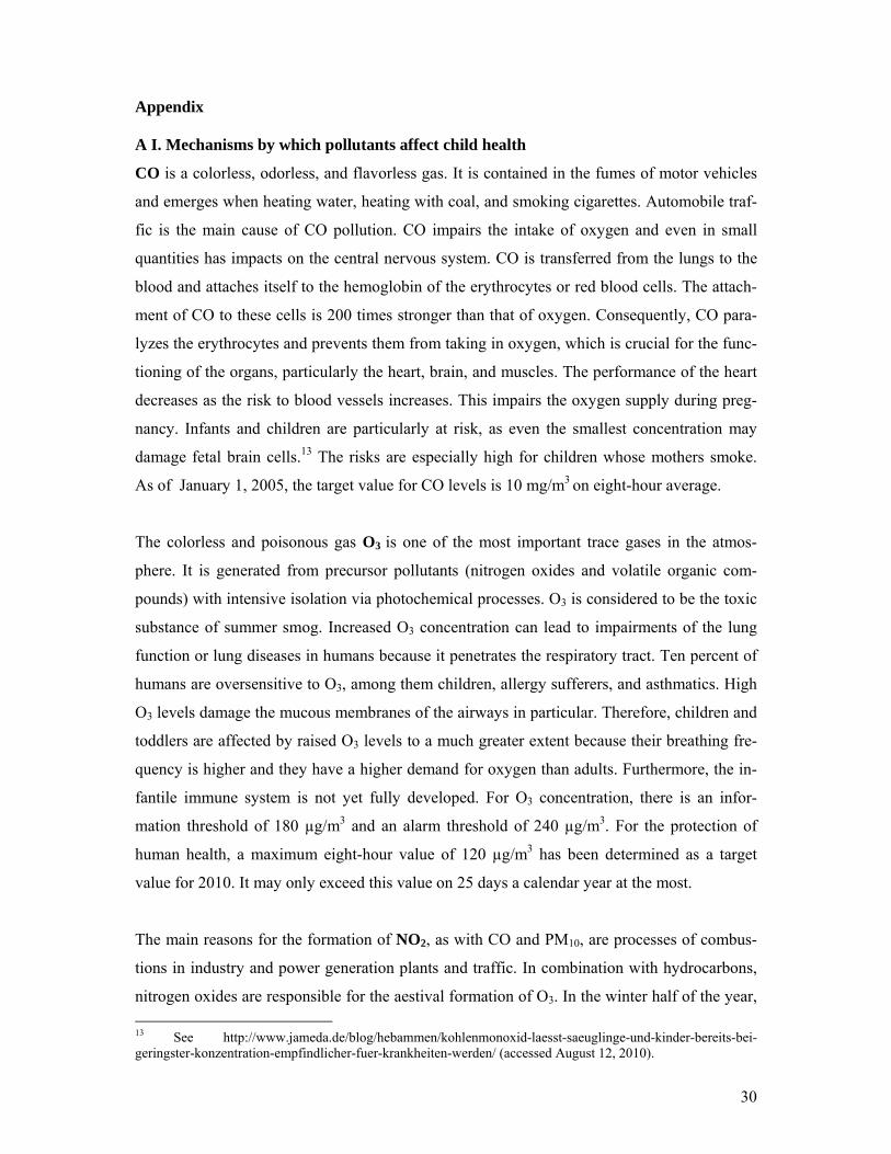
Results for infants. Table 1 presents the estimation results for the first age group for all five pollu-

tants and all specifications. All three models include the variables described in Table A1, but only

the various effects of the five air pollution measures on birth length, birth weight, fetal growth, and

later disorders are shown.

Table 1 about here.

As indicated in Table 1, CO exposure during pregnancy and just before birth has a significantly

negative impact on fetal growth and birth weight in Model 3 (equation 3a). Hence, it becomes ap-

parent that CO impairs the ability of the blood to transport oxygen and thus to supply oxygen to the

fetus. An increase in the average CO exposure during the month before birth causes, on average, a

289 gram lower birth weight. Here, the impact on birth weight and fetal growth towards the end of

pregnancy appears to be significantly higher than at earlier stages. Taking into consideration the

mean value of CO exposure during pregnancy the total impact is less than 200 grams. The effect is

significant independent of the pollutant measure; it applies for the means and the latent factors.

This outcome is in line with the results reported by Currie et al. (2009), which show that pollution

in the last trimester is most important for infant health. For O3, the effect of exposure appears to be

negative throughout the entire pregnancy, not only at the end. This holds for birth length, birth

weight, and fetal growth. However, some of the effects are only significant on the 10% level, and

not robust with respect to the pollutant measures used. Once the latent measures are used, only the

effect on fetal growth stays significant. For a higher exposure to NO2 and SO2, we find a negative

impact on birth length. Moreover, the higher the amount of SO2, the higher the probability that the

child will have disorders in the first year. Overall, the negative impact of SO2 on birth length is

greater than that of NO2. Moreover, the results on these two polluntant measures are sensitive to the

10 For all models with latent factors, the standard errors were bootstrapped with 500 replications.

17

pollutant measures used. For PM10, we find no impact in most models and specifications that ac-

count for both unobservable neighborhood effects and unobservable effects within the family.

However, we find a positive mean effect of fine particles at birth on fetal growth and birth weight.

The same implausible effect is reported in Currie et al. (2009). A possible explanation for these

mixed results could be that fine particles tend to cause long-term respiratory illnesses (cancer,

pneumoconiosis), which is certainly harmful for fetuses but cannot easily be identified due to the

variation in our model, which is designed to cover the short term. Moreover, there are some corre-

lations in the models that do not control for unobservable effects within the family.

Table 2 about here.

Table 2 shows how the overall air pollution outside of the household impacts child health in the first

year when parental smoking is controlled for. In most models, a pattern of ambient air pollution

from Table 1 emerges where no impact of parental smoking behavior is observable—with the ex-

ception of the negative effects for the PM10 models—when controlling for the unobservable neigh-

borhood and family effects. This effect may result from the smaller variation within the family with

regard to parental smoking behavior. To obtain further insights, we estimate models covering paren-

tal smoking exposure only.11 Almost all these models show that the mother’s smoking has a nega-

tive impact on birth outcomes, whereas the father’s smoking and the resulting passive smoking by

the mother during pregnancy do not seem to be so harmful. However, the smoking intensity and,

consequently, one aspect of the air quality in the home also impair fetal growth and reduce the birth

weight. But obviously, this effect does not appear in the models with the outdoor pollutants.

In light of these results, it is interesting to see whether outdoor pollution interacts with parental

smoking behavior (see, e.g., Currie et al., 2009). Thus we also estimate models including an inter-

action term. Mostly the interaction terms are not significant. Nevertheless, almost all significant

coefficients have the expected sign, which means, for instance, that a higher level of PM10, which

accompanies parental smoking behavior, reduces fetal growth or increases the probability of having

any disorder (see Table A2).

Results for toddlers. The effects of the five air pollutants on selected health indicators for toddlers

are depicted in Table 3. Analogously to the models for infants, in model (1) we present OLS results;

in model (2) we control for county fixed effects; and in model (3) we also take family fixed effects

11 Available from the authors upon request.

18

into account. In comparison to the results for the younger children, it has to be considered that this

sample consists of around 300 observations fewer and that the temporal variation (2005 to 2007)

and variation within the family is significantly smaller. For this reason, identifying air pollution

effects is particularly difficult in Models 2 and 3 and we therefore do discuss the results of Model 1

as well. In most specifications, O3 exposure leads to an increased probability of falling ill with

bronchitis or respiratory diseases, or of having some impairment. This view is confirmed for some

specifications and is partly robust when an area fixed effect and a family fixed effect are taken into

account. The latter effect remains significant for the probability of having bronchitis. While the

correlations are hardly sensitive to changes in the pollutant measures in the OLS models, they are

sensitive, to some extent, to changes in the models controlling for county and family fixed effect.

PM10 also increases the probability of contracting bronchitis or respiratory diseases. The latter effect

even occurs in the models that account for area and family fixed effects and can be measured for

latent and non-latent pollutant measures. In contrast, we find mixed results for the effects of CO,

SO2, and NO2 on toddler health

Table 3 about here.

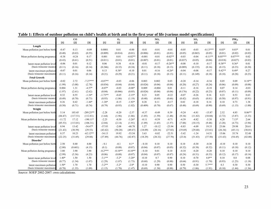
Table 4 shows the impact of the overall air pollution on child health at the age of two to three

years, also controlling for parental smoking behavior. Consistent with the results from Table 3,

higher O3 exposure leads to an increased likelihood of respiratory diseases, bronchitis, or other im-

pairments. But the results are not statistically significant when we control for county and family

fixed effects. The models in Table 4 show no effect of parental smoking. If we again only regress

on mothers` and fathers` smoking behavior and the control variables the results12 suggest that pa-

rental smoking does not have a significant impact on the health measures at this age, with the ex-

ception that the probability of having bronchitis or a disorder increases if the father smokes.

Table 4 about here.

In line with the models for infants, we also estimate models with an interaction effect between out-

door pollution and parental smoking behavior (Table A3). Again, the results do not change signifi-

cantly. For some pollutants, the interaction effects are significant. For example, a high level of

PM10 in combination with parental smoking increases the probability of croup syndrome and other

disorders of toddlers.

12 Available from the authors upon request.

19

6 Conclusion

It has become a generally accepted fact that air pollution should be reduced for numerous reasons,

including human health. The health of children is of particular importance here, both because of

children’s higher short-term vulnerability to pollutants and because early exposure has longer-term

impacts on their mental and physical development and skill formation. In recent years, economists

have begun to analyze the impacts of air pollution on child health, primarily in the US. This poses

various challenges, first and foremost that of finding appropriate health and air pollution measures

that make it possible to estimate the causal impact of air pollution accurately. Two further obstacles

are the presence of confounding factors brought about through residential sorting and the lack of

health measures that capture the range of morbidities purportedly related to pollution.

We cope with the aforementioned problems by utilizing representative German data to analyze the

effect of air pollution on child health using county and family fixed effects. We employ different

health measures such as anthropometric measures and the occurrence of impairments such as bron-

chitis that are known to have some correlation with air pollution. A further advantage of our study is

the wide range of pollution measures used, including accurate measures for five different pollutants

(CO, NO2, SO2, O3, and PM10) collected on a (half-) hourly basis.

Our analysis covers two age groups, infants and toddlers, to provide indications as to which age

group shows the more pronounced effects. Moreover, our approach allows us to analyze the effects

of different pollutants. It therefore gives further evidence as to which pollutants matter most for

child health and which are of minor importance. Apart from the study by Lüchinger (2009), this is

the only study to date focusing on a potential causal relationship between pollution and child health

in Europe. In general, air pollution is less of a problem in Germany than in the United States, alt-

hough it remains a major concern in densely populated urban areas.

Our estimation results show that air pollution matters, particularly at birth. CO levels affect fetal

growth and birth weight. As traffic is the main cause of CO air pollution, policies and measures

making cars more environmentally friendly may therefore lead to improvements in child health. The

extreme vulnerability of infants and young children to high CO levels makes such efforts especially

important, as even the smallest concentration of this pollutant may damage fetal brain cells.

20

Furthermore, our estimations show evidence that O3 levels affect the probability of children having

some type of disorder. O3 is generally a major toxic agent in summer smog. Therefore, infants and

toddlers are affected much more than adults by increased O3 levels because their breathing frequen-

cy and thus their demand for oxygen is higher. Furthermore, since the infant immune system is not

yet fully developed, areas with a high risk of summer smog may be dangerous for very young chil-

dren. Similar results are found for the SO2 level. Oxidation processes of SO2 lead to acid rain.

Again, areas with elevated SO2 levels pose a health risk for infants. With our older group of chil-

dren, the two- to three-year-olds, we mainly find effects for O3 levels, which increase the probabil-

ity of having bronchitis or respiratory disease. Thus, summer smog might be one cause of these

types of impairments.

From a policy perspective, on the one hand, our results confirm the importance of efforts to raise

awareness among parents of infants of the negative consequences of smoking on the health and

development of their child. Potential activities include public campaigns and consultations with

pediatricians and experts. On the other hand, our results underscore the need for further efforts on

the regional and national level to reduce CO and O3 levels in particular. Since these pollutants are

higher in cities, environmental policies should focus on reducing these pollutants in these areas in

order to improve child health. Here, the potential child health benefits of further reductions in air

pollution appear particularly high.

Nevertheless, our study could benefit from further research using even more precise pollution

measures—for example, personal air quality monitors that can be worn by study participants. Until

such data become available for large representative data sets, however, the findings obtained

should be interpreted as conservative estimates that may underestimate the actual effects (see Cur-

rie et al. 2009).

21

Literature

Case, A., Lubotsky, D. and C.Paxson, 2002. Economic Status and Health in Childhood: The Ori-

gins of the Gradient. American Economic Review 92(5), 1308- 1334.

Cawley, J. and C. K. Spiess, 2008. Obesity and Skill Attainment in Early Childhood. in: Economics

and Human Biology 6(3), 388–397.

Chay, K., and M. Greenstone, 2003. The impact of air pollution on infant mortality: Evidence form

geographic variation in pollution shocks induced by a recession. in: Quarterly Journal of

Economics 118(3), 1121-1167.

Coneus, K., and C. K. Spiess, 2011. The Intergenerational Transmission of Health in Early Child-

hood, Economics and Human Biology, forthcoming.

Currie, J. and M. Neidell, 2005. Air Pollution and Infant Health: What Can We Learn from Cali-

fornia’s Recent Experience? Quarterly Journal of Economics 120(3), 1003-1030.

Currie, J., Neidell, M. and J. Schmieder, 2009. Air Pollution and Infant Health: Lessons from New

Jersey. Journal of Health Economics 28(3), 688-703.

Currie, J., 2009. Healthy, Wealthy, and Wise: Socioeconomic Status, Poor Health in Childhood,

and Human Capital Development. Journal of Economic Literature 47(1), 87-122.

Currie, J. and R. Walker, 2011. Traffic Congestion and Infant Health: Evidence from E-Z-Pass, in:

American Economic Journal: Applied Economics 3, 65–90.

Currie, J.. M. Greenstone, and E. Moretti, 2011. Responses to environmental regulation. Superfund

Cleanups and Infant Health, in: American Economic Review 101 (3): 435–441

Currie, J., 2011. Inequality at Birth: Some Causes and Consequences, in: American Economic Re-

view: Papers & Proceedings 101 (3), 1–22.

Dunkelberg, A. and C. K. Spiess, 2009. The Impact of Child and Maternal Health Indicators on

Female Labor Force Participation after Childbirth - Evidence for Germany. in: Journal of

Comparative Family Studies 40, 119–138.

Frank, I.E., Todeschini, R., 1994. The data analysis handbook. Amsterdam: Elsevier.

Jöreskog, K.G., 1967. Some Contributions to Maximum Likelihood Factor Analysis. Psychometrica

32, 443-482.

Kaiser, H. F., 1960. The application of electronic computers to factor analysis. Educational and

Psychological Measurement 20, 141-151

Kim, Y. S., 2009. The Impact of Rainfall on Early Child Health, November, 2009, mimeo.

Kurth, B.-M. et al., 2008. The challenge of comprehensively mapping children’s health in a nation-

wide health survey: Design of the German KiGGS-Study. in: BMC Public Health 8, 196.

22

Kvedaras V. and A. Račkauskas, 2010. Regression Models with Variables of Different Frequen-

cies: the Case of a Fixed Frequency Ratio, in: Oxford Bulletin of Economics and Statistics

72, 600-620.

Lleras-Muney, A., 2010. The Needs of the Army. Using Compulsory Relocation in the Military to

Estimate the Effect of Air Pollution on Children`s Health, Journal of Human Resources

45(3), 547-590.

Lüchinger, S., 2009. Air Pollution and Infant Mortality: A Natural Experiment from Power Plant

Desulfurization, Working Paper.

Neidell, M., 2004. Air Pollution, Health and Socio-Economic Status: The Effect of Outdoor Air

Quality on Childhood Asthma. Journal of Health Economics 23(6), 1209-1236.

Moretti, E. and M. Neidell, 2011. Pollution, Health, and Avoidance Behavior. Evidence from the

Ports of Los Angeles. Journal of Human Resources 46(1), 154-175.

Oreopoulus, P, Stabile, M., Walld, R. and L. Roos, 2008. Short, Medium, and Long Term Conse-

quences of Poor Infant Health: An Analysis using Siblings and Twins. Journal of Human

Resources 43(1), 88-138.

Trendafilov, N. T. and S. Unkel., 2011. Exploratory factor analysis of data matrices with more var-

iables than observations, Journal of Computational and Graphical Statistics (to appear)..

Wagner, G.G., Frick, J.R., and J. Schupp., 2007. The German Socio-Economic Panel Study

(SOEP) – Scope, Evolution, and Enhancements. Schmollers Jahrbuch 127, 139-169.

23

Table 1: Effects of outdoor pollution on child’s health at birth and in the first year of life (various model specifications) CO O3 NO2 SO2 PM10 [1] [2] [3] [1] [2] [3] [1] [2] [3] [1] [2] [3] [1] [2] [3]

Length Mean pollution just before birth -0.47 0.13 -0.09 0.0001 0.01 -0.00 -0.01 -0.01 -0.01 -0.05 -0.03 -0.13*** 0.03* 0.03* 0.01

(0.48) (0.63) (0.55) (0.009) (0.014) (0.01) (0.006) (0.01) (0.01) (0.05) (0.065) (0.05) (0.01) (0.02) (0.02) Mean pollution during pregnancy -0.38 -0.24 0.17 0.001 0.01 -0.02** -0.001 -0.01 -0.02** -0.03 -0.04 -0.11** 0.05*** 0.07*** 0.02

(0.43) (0.61) (0.51) (0.011) (0.01) (0.01) (0.007) (0.01) (0.01) (0.037) (0.05) (0.04) (0.018) (0.027) (0.02)

latent mean pollution level (basis trimester means)

-0.06 0.01 0.12 0.06 0.38 -0.16 -0.01 -0.17 -0.26** -0.08 -0.10 -0.17 0.38** 0.36* 0.01 (0.11) (0.16) (0.14) (0.246) (0.32) (0.24) (0.11) (0.18) (0.13) (0.089) (0.135) (0.16) (0.15) (0.23) (0.20)

latent maximum pollution (basis trimester maximum)

-0.07 0.01 0.06 0.13 0.38* -0.10 0.01 -0.16 -0.26* -0.04 -0.08 -0.17 0.42** 0.49* 0.27 (0.11) (0.16) (0.14) (0.21) (0.29) (0.21) (0.11) (0.18) (0.13) (0.11) (0.149) (0.18) (0.18) (0.28) (0.23)

Fetal Growth Mean pollution just before birth -0.02 2.72 -7.27*** -0.07** -0.03 -0.06 0.003 0.002 0.03 -0.20 -0.14 -0.34 0.05 0.09 0.18**

(1.99) (3.08) (2.78) (0.034) (0.04) (0.04) (0.024) (0.04) (0.04) (0.20) (0.27) (0.24) (0.06) (0.09) (0.08) Mean pollution during pregnancy 0.004 1.31 -4.57* -0.07* -0.03 -0.08* 0.009 -0.004 0.01 -0.11 -0.16 -0.18 0.07 0.14 -0.01

(1.97) (2.61) (2.62) (0.04) (0.046) (0.05) (0.024) (0.04) (0.04) (0.176) (0.22) (0.23) (0.07) (0.11) (0.09)

latent mean pollution level (basis trimester means)

0.32 0.55 -1.34* -1.73** -0.65 -2.15* 0.23 0.05 -0.22 -0.07 -0.26 0.16 0.23 0.53 0.63 (0.49) (0.70) (0.73) (0.93) (1.06) (1.19) (0.40) (0.69) (0.66) (0.42) (0.65) (0.81) (0.58) (0.97) (0.91)

latent maximum pollution (basis trimester maximum)

0.26 0.42 -1.44* -1.20* -0.15 -1.92* 0.28 0.11 -0.17 0.02 -0.18 0.14 0.10 0.73 1.38 (0.50) (0.71) (0.74) (0.79) (0.93) (1.02) (0.409) (0.70) (0.67) (0.48) (0.69) (0.90) (0.69) (1.15) (1.00)

Weight Mean pollution just before birth 5.14 103.45 -289.25** -2.28 -0.20 -2.57 -0.37 -0.49 0.39 -9.24 -4.81 -15.87 2.52 4.85 8.06**

(84.47) (117.51) (112.81) (1.64) (1.96) (1.86) (1.05) (1.59) (1.48) (9.34) (11.82) (10.04) (2.72) (3.87) (3.33) Mean pollution during pregnancy -11.72 17.12 -190.11* -2.25 -0.50 -3.26* -0.11 -0.59 -0.71 -4.39 -4.82 -5.38 4.28 7.13* 2.64

(85.53) (113.01) (106.31) (2.04) (2.14) (1.91) (1.09) (1.65) (1.57) (7.88) (10.15) (9.48) (3.28) (4.73) (3.94)

latent mean pollution level (basis trimester means)

8.94 13.42 -54.47* -57.93 -2.08 -68.78 1.27 -10.12 -23.94 -8.83 -4.09 19.33 23.06 29.98 28.61 (21.43) (30.59) (29.53) (43.62) (50.20) (49.67) (18.09) (28.16) (27.02) (19.69) (29.68) (33.81) (26.34) (45.11) (38.01)

latent maximum pollution (basis trimester maximum)

8.37 10.23 -62.12** -34.13 19.92 -53.54 3.63 -8.02 -22.51 -5.42 -1.24 14.51 15.06 35.74 52.48 (22.25) (31.05) (29.88) (37.89) (44.76) (42.87) (18.29) (28.32) (27.70) (23.0) (31.83) (37.50) (31.63) (54.45) (42.08)

Disorder1 Mean pollution just before birth 2.50 0.40 4.00 - 0.1 -0.1 0.1* - 0.10 0.10 0.10 0.10 -0.30 -0.30 -0.10 0.10 0.10

(2.80) (0.601) (4.15) (0.1) (0.08) (0.07) (0.04) (0.07) (0.05) (0.32) (0.38) (0.32) (0.11) (0.18) (0.12) Mean pollution during pregnancy 3.80 3.90 3.90 -0.2*** -0.10** -0.10** - 0.10 0.01 0.10 -0.10 -0.20 -0.20 0.10 0.10 0.10

(2.99) (5.36) (4.23) (0.06) (0.08) (0.07) (0.04) (0.07) (0.87) (0.24) (0.31) (0.33) (0.12) (0.17) (0.14)

latent mean pollution level (basis trimester means)

1.40* 1.50 1.50 -3.1** -3.2* -3.20* -0.10 0.7 0.90 0.10 -0.70 4.0** 0.10 0.8 0.08 (0.77) (1.34) (1.07) (1.29) (1.87) (1.73) (0.68) (1.29) (0.88) (0.64) (0.91) (1.70) (0.93) (1.25) (1.18)

latent maximum pollution (basis trimester maximum)

1.50* 1.70 1.70 -3.2** -3.2* -2.8* -0.10 0.90 0.90 0.50 -0.30 5.7*** 0.3 0.30 0.30 (0.78) (1.35) (1.09) (1.15) (1.70) (1.47) (0.69) (1.30) (0.88) (0.79) (1.06) (1.91) (0.10) (1.44) (1.36)

Source: SOEP 2002-2007: own calculations.

24

Notes: All coefficients are from different regressions. Standard errors are in parentheses. *indicates statistical significance at the 10% level, ** at the 5% level, *** at the 1% level. All regressions include indicators of mother’s education, age, income, municipality size, immigration background, sex of the child, birth order, month and year dummies. Model [1] OLS, refers to equation (1a), model [2] Area fixed effect, refers to equation (2a) and model [3] Area and family fixed effect, refers to equation (3a). Sample size varies between 1,154 and 1,268 observations. 1Coefficient and standard errors are multiply with 100.

25

Table 2: Effects of outdoor pollution and parental smoking on child’s health at birth and in the first year of life (various model specifica-tions)

iCO iO3 iNO2 iSO2 iPM10 [1] [2] [3] [1] [2] [3] [1] [2] [3] [1] [2] [3] [1] [2] [3] Length outdoor (latent)i -0.04 0.08 -0.10 -0.30** -0.18 -0.49 -0.07 -0.25 -0.26* -0.17 -0.14 -0.34** 0.36** 0.29 -0.25 (0.12) (0.18) (0.15) (0.148) (0.19) (0.30) (0.11) (0.18) (0.14) (0.11) (0.16) (0.16) (0.16) (0.24) (0.21) smoking (latent) -0.39** -0.37* 0.20 0.19 0.40 -0.05 -0.33** -0.32* -0.11 -0.31** -0.21 -0.03 -0.46** -0.59** -1.11***

(0.16) (0.23) (0.35) (0.24) (0.33) (0.25) (0.146) (0.20) (0.33) (0.16) (0.22) (0.31) (0.18) (0.29) (0.33)

Fetal growth outdoor (latent)i 0.52 0.85 -1.65** -1.64*** -1.05 -2.16 0.03 -0.15 -0.29 -0.21 -0.42 -0.20 0.02 0.40 0.65 (0.42) (0.72) (0.79) (0.59) (0.80) (1.59) (0.42) (0.75) (0.72) (0.42) (0.75) (0.87) (0.58) (0.96) (0.96) smoking (latent) -1.81*** -1.25 -0.46 -1.03 -0.53 -1.82 -1.49** -1.19 0.40 -1.38** -0.64 -0.09 -2.34*** -2.24** -3.82**

(0.67) (0.97) (1.91) (0.96) (1.07) (1.28) (0.60) (0.83) (1.77) (0.66) (0.93) (1.72) (0.78) (1.19) (1.55)

Birth weight outdoor (latent)i 19.86 25.08 -77.92** -68.60*** -46.15 -62.17 -10.21 -19.22 -22.04 -14.65 -6.61 -8.35 11.20 11.17 10.27 (19.35) (33.38) (32.81) (24.58) (33.27) (65.50) (18.59) (30.74) (30.20) (19.615) (32.27) (37.04) (26.37) (43.86) (40.92) smoking (latent)

-77.13*** -62.54* 23.30 -29.45 12.56 -51.43 -67.86*** -62.37* 51.02 -57.15** -33.79 35.73 -101.86***-114.40**-

206.77***

(27.28) (40.56) (77.23) (44.97) (52.79) (53.77) (24.99) (34.38) (72.45) (28.12) (38.70) (71.80) (31.33) (49.76) (65.97)

Disorder1 outdoor (latent)i 1.50* 1.20 1.20 -0.5 -0.1 -1.0 -0.10 1.10 1.1* 0.40 0.10 0.10 0.20 0.60 0.60 (0.81) (1.52) (1.09) (1.14) (1.45) (1.07) (0.73) (1.39) (0.90) (0.71) (0.098) (1.03) (0.99) (1.40) (1.22) smoking (latent) 0.10 1.40 1.40 -3.20** -3.40* -3.40* 0.50 0.90 0.90 0.40 1.1 1.10 0.10 0.31 0.30 (1.08) (1.57) (1.16) (1.33) (1.94) (1.78) (1.19) (1.54) (1.08) (1.32) (1.79) (1.21) (1.47) (1.96) (1.30)

Source: SOEP 2002-2007: own calculations. Notes: All coefficients are from different regressions. Standard errors are in parentheses. *indicates statistical significance at the 10% level, ** at the 5% level, *** at the 1% level. All regressions include indicators of mother’s education, age, income, municipality size, immigration background, sex of the child, birth order, month and year dummies. Model [1] OLS, refers to equation (1b), model [2] Area fixed effect, refers to equation (2b) and model [3] Area and family fixed effect, refers to equation (3b). Sample size varies between 1,154 and 1,268 observations.1Coefficients and standard errors are multiply with 100.

26

Table 3: Effects of outdoor pollution on child’s health at two to three years of age (various model specifications, coefficients and standard er-rors multiplied by 100)

CO O3 NO2 SO2 PM10 [1] [2] [3] [1] [2] [3] [1] [2] [3] [1] [2] [3] [1] [2] [3]

Bronchitis mean year pollution -5.40 -5.80 -8.0 0.20** 0.10 0.30 -0.10 0.10 -0.20 -0.20 -0.50 1.0 -0.40* -0.40 0.50

(6.62) (11.98) (13.8) (0.07) (0.11) (0.2) (0.06) (0.13) (0.15) (0.52) (1.12) (1.6) (0.23) (0.52) (0.4) mean pollution at interview -2.10 -7.60 -5.9 0.1* 0.10 0.20 -0.10 0.10 -0.20 0.10 0.40 0.90 -0.10 -0.10 0.20

(6.11) (11.09) (1.5) (0.08) (0.14) (0.2) (0.06) (0.13) (0.2) (0.46) (1.11) (1.4) (0.17) (0.41) (0.3) three-year mean -7.70 -17.4 -21.1 0.20** 0.20 0.70** 0.10 -0.10 -0.30 0.10 0.10 1.40 -0.20 -0.30 -0.10

(5.96) (10.72) (20.0) (0.11) (0.27) (0.3) (0.08) (0.19) (0.2) (0.08) (1.27) (1.6) (0.26) (0.34) (0.4) latent pollution intensity -0.80 -1.50 -2.7 2.20** 1.60 1.80 -0.40 0.30 -3.50 -0.50 -0.60 1.80 -2.30 -1.70 5.40

(1.13) (2.15) (2.8) (1.06) (1.83) (2.8) (1.00) (2.27) (2.6) (1.03) (2.29) (3.5) (1.55) (3.25) (3.3) Latent pollution intensity at interview -1.10 -1.50 -2.8 2.0** 0.90 2.90 -0.50 0.30 -3.0 -1.10 -1.10 2.70 -2.60* -2.0 3.80

(1.23) (2.17) (2.5) (0.9) (1.51) (2.8) (1.00) (0.28) (2.7) (0.96) (2.31) (3.3) (1.52) (3.17) (3.1) Croup syndrome

mean year pollution 6.50 5.50 -26.0 -0.01 0.10 0.30 -0.10 -0.10 -0.20 -0.10 -0.40 -2.70 -0.10 -0.30 -0.50 (6.92) (9.68) (18.4) (0.07) (0.17) (0.3) (0.06) (0.15) (0.2) (0.52) (1.18) (2.2) (0.27) (0.54) (1.1)

mean pollution at interview 4.50 3.60 -21.0 0.10 0.10 -0.10 0.10 -0.10 -0.20 0.10 0.30 -1.60 -0.20 -0.20 0.70 (5.66) (7.79) (18.0) (0.98) (0.13) (0.3) (0.06) (0.13) (0.2) (0.49) (1.07) (1.9) (0.22) (0.41) (0.8)

three-years mean 4.20 -3.10 -25.0 0.10 0.30 0.30 0.10 -0.10 0.20 0.10 1.70 1.70 -0.20 -0.50 0.80 (5.59) (12.19) (25.0) (0.08) (0.31) (0.4) (0.10) (0.22) (0.3) (0.08) (1.43) (2.2) (0.23) (0.53) (0.8)

latent pollution intensity 6.0*** 0.60 -5.20 0.40 1.60 0.10 0.20 -1.60 -2.50 -0.30 -1.30 -10.0* -1.60 0.60 7.0 (1.16) (1.79) (3.8) (1.09) (2.0) (3.6) (1.14) (2.44) (3.7) (1.27) (2.77) (5.0) (1.58) (2.72) (9.0)

latent pollution intensity at interview 1.00 0.80 -5.0 -0.10 0.30 2.70 -0.20 -1.20 -2.60 -0.30 -1.0 -6.10 -1.10 -0.20 6.0 (1.33) (1.69) (3.5) (1.0) (1.51) (3.7) (1.11) (2.58) (3.8) (1.09) (2.50) (4.8) (1.73) (3.14) (7.3)

Respiratory disease mean year pollution -6.90 -8.0 -3.30 0.30*** 0.20 0.20 -0.10 0.10 -0.10 -1.10* -0.90 -0.40 -0.50 -0.40 1.50*

(8.51) (13.91) (1.9) (0.10) (0.18) (0.3) (0.07) (0.15) (0.2) (0.63) (1.20) (2.2) (0.31) (0.57) (0.8) mean pollution at interview -3.10 -12.0 0.017 0.29* 0.18 0.10 -0.10 0.10 -0.10 -0.70 0.10 -0.10 -0.20 -0.10 0.80

(8.44) (13.63) (0.20) (0.14) (0.24) (0.3) (0.07) (0.15) (0.2) (0.53) (1.22) (2.0) (0.21) (0.40) (0.6) three-year mean -11.20 -29.0** -19.1 0.30** 0.20 0.50 -0.10 0.10 -0.20 -0.10 0.40 2.60 -0.20 -0.30 0.30

(8.19) (13.68) (27.0) (0.15) (0.35) (4.4) (0.09) (0.21) (2.6) (0.09) (1.56) (2.2) (0.33) (0.72) (0.7) latent pollution intensity -1.20 -3.40 -0.03 3.6*** 3.10 -0.30 -0.50 1.50 -2.20 -3.10** -2.5 -3.70 -2.50 -1.10 0.18***

(1.73) (2.83) (0.039) (1.38) (2.38) (4.1) (1.20) (2.62) (3.8) (1.27) (2.69) (5.0) (1.94) (3.57) (0.06) latent pollution intensity at interview -1.40 -2.3 -0.021 3.1** 3.10 2.30 -0.60 1.40 -1.80 -3.0** -1.70 -0.50 -2.80 -2.0 9.00

(1.62) (2.48) (0.035) (1.40) (2.38) (4.1) (1.22) (2.63) (3.9) (1.21) (2.47) (4.7) (1.99) (3.48) (5.7)

Disorder mean year pollution 3.80 -9.70 -16.7 0.40** 0.3 0.7* 0.1 0.20 -0.2 -0.4 -0.7 -0.044 0.50 -0.30 -0.80

27

(11.73) (21.84) (25.0) (0.16) (0.28) (0.4) (0.11) (0.19) (0.28) (1.09) (1.98) (0.028) (0.43) (0.64) (1.0) mean pollution at interview 3.0 -14.0 -11.0 0.5*** 0.30 0.30 0.10 0.30 -0.10 -1.0 -0.80 0.017 0.20 -0.30 -1.0

(11.56) (21.64) (27.0) (0.162) (0.28) (0.4) (0.10) (0.18) (0.3) (0.93) (1.80) (0.025) (0.36) (0.54) (0.8) three-year mean 0.10 -25.40 -15.0 0.40* 0.40 0.60 0.10 0.10 0.70** 0.10 0.40 0.006 0.30 -0.30 2.0**

(13.23) (23.0) (36.0) (0.2) (0.4) (0.6) (0.14) (0.26) (0.4) (0.14) (2.36) (0.03) (0.38) (0.70) (0.8) latent pollution intensity 1.80 -0.2 -0.6 6.6*** 6.20* 6.0 1.50 4.0 -0.4 -1.0 -2.2 0.085 0.60 -2.0 -12.0

(2.29) (4.69) (5.7) (1.97) (3.46) (5.5) (1.82) (3.38) (4.7) (2.32) (4.47) (0.06) (2.63) (4.05) (8.5) latent pollution intensity at interview 1.60 -0.70 -2.0 4.90** 2.20 8.0 1.70 4.40 -2.0 -1.0 -1.50 0.08 2.40 -0.90 0.80

(2.33) (4.38) (5.0) (2.14) (3.68) (5.3) (1.88) (3.41) (4.6) (2.30) (4.17) (0.059) (2.70) (3.90) (6.8)

Source: SOEP 2002-2007: own calculations. Notes: All coefficients are from different regressions. Standard errors are in parentheses. *indicates statistical significance at the 10% level, ** at the 5% level, *** at the 1% level. All regressions include indicators for mother’s education, age, income, municipality size, immigration background, sex of the child, birth order, birth weight, child’s age in months, month and year dummies. Model [1] OLS, refers to equation (1a), model [2] Area fixed effect, refers to equation (2a) and model [3] Area and family fixed effect, refers to equation (3a). Sample size varies between 629 and 775 observations.

28

Table 4: Effects of outdoor pollution and parental smoking on child’s health at two to three years of age (various model specifications, coeffi-cients and standard errors multiplied by 100)

CO O3 NO2 SO2 PM10 [1] [2] [3] [1] [2] [3] [1] [2] [3] [1] [2] [3] [1] [2] [3]

Bronchitis outdoor (latent) -0.60 -1.00 -0.40 2.30** 1.50 1.40 -0.20 0.60 -3.20 -0.20 -0.30 4.80 -2.70 -2.8 6.0* (1.13) (2.16) (2.48) (1.08) (1.86) (2.93) (1.04) (2.31) (2.51) (1.08) (2.00) (3.17) (1.7) (3.63) (3.56) smoking (latent) -0.50 0.90 -2.0 0.30 -2.20 -1.80 0.30 -2.0 -1.40 -0.30 -2.0 -1.90 1.70 -2.0 12.0 (2.12) (3.63) (9.22) (1.82) (3.12) (7.97) (1.92) (3.32) (7.28) (2.06) (3.46) (10.41) (2.81) (5.23) (8.15) Croup syndrome outdoor (latent) 0.50 1.20 -4.60 0.50 2.0 -2.0 -0.20 -1.60 -2.10 -0.50 -1.40 -10.0** -2.20 -0.40 5.60 (1.15) (1.83) (4.00) (1.18) (1.96) (3.65) (1.11) (2.56) (3.74) (1.02) (2.52) (4.61) (1.60) (2.61) (9.37) smoking (latent) -0.50 0.80 -11.7 0.50 0.10 -0.70 1.10 -0.10 -4.20 0.60 -0.20 -9.0 -0.20 1.50 -5.70 (1.67) (2.59) (14.84) (1.63) (2.14) (1.00) (1.71) (2.42) (10.0) (1.73) (2.56) (15.16) (2.23) (3.50) (21.49)Respiratory disease outdoor (latent) -1.10 -3.10 -1.30 3.5** 2.40 -0.60 -0.20 1.60 -1.70 -2.70** -2.0 -0.50 -3.0 -2.0 19.0*** (1.71) (3.02) (3.79) (1.42) (2.42) (4.27) (1.22) (2.67) (3.78) (1.30) (2.55) (4.71) (2.01) (4.01) (6.75) smoking (latent) -1.20 -0.30 -3.80 -0.90 -2.30 -4.70 -0.60 -1.70 -5.70 -1.80 -2.60 -0.90 0.10 -0.70 1.80 (2.23) (4.17) (14.07) (1.39) (3.21) (11.60) (2.08) (3.65) (10.97) (2.24) (3.95) (15.49) (3.02) (5.32) (15.48)Disorder outdoor (latent) 1.80 -0.10 -0.60 7.0*** 6.0* 2.00 1.20 3.50 -2.10 -1.10 -1.90 9.0 0.20 -3.0 -1.10 (2.28) (4.86) (6.0) (2.03) (3.59) (5.59) (1.87) (3.51) (4.89) (2.23) (4.25) (5.98) (2.73) (4.14) (9.21) smoking (latent) -1.10 -0.10 0.90 -1.20 0.30 19.0 -0.10 1.80 2.10 0.40 2.40 6.0 4.30 12.0* 14.0 (3.16) (5.58) (22.65) (2.90) (5.18) (15.15) (1.99) (5.11) (14.19) (3.03) (5.33) (19.68) (4.68) (6.38) (21.10) Source: SOEP 2002-2007: own calculations. Notes: All coefficients are from different regressions. Standard errors are in parentheses. *indicates statistical significance at the 10% level, ** at the 5% level, *** at the 1% level. All regressions include indicators of mother’s education, age, income, municipality size, immigration background, sex of the child, birth order, birth weight, child’s age in months, month and year dummies. Model [1] OLS, refers to equation (1b), model [2] Area fixed effect, refers to equation (2b) and model [3] Area and family fixed effect, refers to equation (3b). Sample size varies between 629 and 775 observations.

29

30

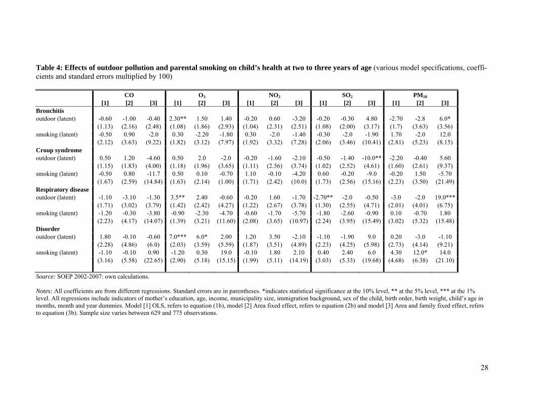
Appendix A I. Mechanisms by which pollutants affect child health

CO is a colorless, odorless, and flavorless gas. It is contained in the fumes of motor vehicles

and emerges when heating water, heating with coal, and smoking cigarettes. Automobile traf-

fic is the main cause of CO pollution. CO impairs the intake of oxygen and even in small

quantities has impacts on the central nervous system. CO is transferred from the lungs to the

blood and attaches itself to the hemoglobin of the erythrocytes or red blood cells. The attach-

ment of CO to these cells is 200 times stronger than that of oxygen. Consequently, CO para-

lyzes the erythrocytes and prevents them from taking in oxygen, which is crucial for the func-

tioning of the organs, particularly the heart, brain, and muscles. The performance of the heart

decreases as the risk to blood vessels increases. This impairs the oxygen supply during preg-

nancy. Infants and children are particularly at risk, as even the smallest concentration may

damage fetal brain cells.13 The risks are especially high for children whose mothers smoke.

As of January 1, 2005, the target value for CO levels is 10 mg/m3 on eight-hour average.

The colorless and poisonous gas O3 is one of the most important trace gases in the atmos-

phere. It is generated from precursor pollutants (nitrogen oxides and volatile organic com-

pounds) with intensive isolation via photochemical processes. O3 is considered to be the toxic

substance of summer smog. Increased O3 concentration can lead to impairments of the lung

function or lung diseases in humans because it penetrates the respiratory tract. Ten percent of

humans are oversensitive to O3, among them children, allergy sufferers, and asthmatics. High

O3 levels damage the mucous membranes of the airways in particular. Therefore, children and

toddlers are affected by raised O3 levels to a much greater extent because their breathing fre-

quency is higher and they have a higher demand for oxygen than adults. Furthermore, the in-

fantile immune system is not yet fully developed. For O3 concentration, there is an infor-

mation threshold of 180 µg/m3 and an alarm threshold of 240 µg/m3. For the protection of

human health, a maximum eight-hour value of 120 µg/m3 has been determined as a target

value for 2010. It may only exceed this value on 25 days a calendar year at the most.

The main reasons for the formation of NO2, as with CO and PM10, are processes of combus-

tions in industry and power generation plants and traffic. In combination with hydrocarbons,

nitrogen oxides are responsible for the aestival formation of O3. In the winter half of the year,

13 See http://www.jameda.de/blog/hebammen/kohlenmonoxid-laesst-saeuglinge-und-kinder-bereits-bei-geringster-konzentration-empfindlicher-fuer-krankheiten-werden/ (accessed August 12, 2010).

31

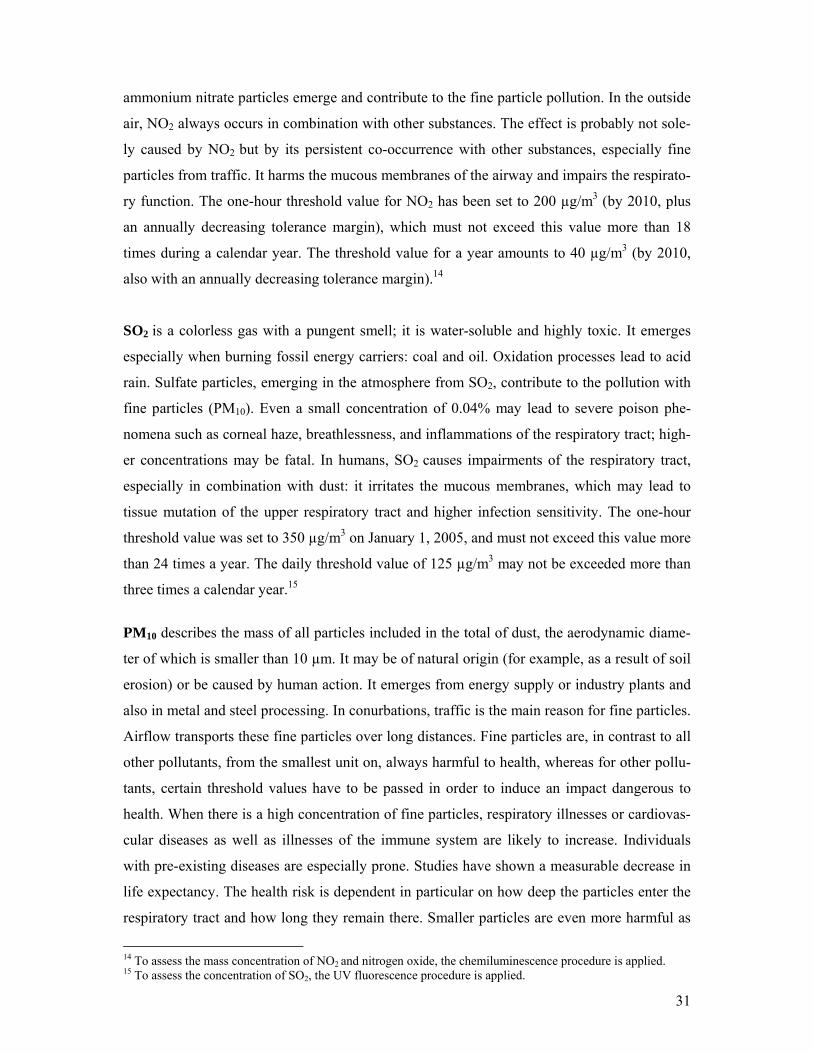
ammonium nitrate particles emerge and contribute to the fine particle pollution. In the outside

air, NO2 always occurs in combination with other substances. The effect is probably not sole-

ly caused by NO2 but by its persistent co-occurrence with other substances, especially fine

particles from traffic. It harms the mucous membranes of the airway and impairs the respirato-

ry function. The one-hour threshold value for NO2 has been set to 200 µg/m3 (by 2010, plus

an annually decreasing tolerance margin), which must not exceed this value more than 18

times during a calendar year. The threshold value for a year amounts to 40 µg/m3 (by 2010,

also with an annually decreasing tolerance margin).14

SO2 is a colorless gas with a pungent smell; it is water-soluble and highly toxic. It emerges

especially when burning fossil energy carriers: coal and oil. Oxidation processes lead to acid

rain. Sulfate particles, emerging in the atmosphere from SO2, contribute to the pollution with

fine particles (PM10). Even a small concentration of 0.04% may lead to severe poison phe-

nomena such as corneal haze, breathlessness, and inflammations of the respiratory tract; high-

er concentrations may be fatal. In humans, SO2 causes impairments of the respiratory tract,

especially in combination with dust: it irritates the mucous membranes, which may lead to

tissue mutation of the upper respiratory tract and higher infection sensitivity. The one-hour

threshold value was set to 350 µg/m3 on January 1, 2005, and must not exceed this value more

than 24 times a year. The daily threshold value of 125 µg/m3 may not be exceeded more than

three times a calendar year.15

PM10 describes the mass of all particles included in the total of dust, the aerodynamic diame-

ter of which is smaller than 10 µm. It may be of natural origin (for example, as a result of soil

erosion) or be caused by human action. It emerges from energy supply or industry plants and

also in metal and steel processing. In conurbations, traffic is the main reason for fine particles.

Airflow transports these fine particles over long distances. Fine particles are, in contrast to all

other pollutants, from the smallest unit on, always harmful to health, whereas for other pollu-

tants, certain threshold values have to be passed in order to induce an impact dangerous to

health. When there is a high concentration of fine particles, respiratory illnesses or cardiovas-

cular diseases as well as illnesses of the immune system are likely to increase. Individuals

with pre-existing diseases are especially prone. Studies have shown a measurable decrease in

life expectancy. The health risk is dependent in particular on how deep the particles enter the

respiratory tract and how long they remain there. Smaller particles are even more harmful as

14 To assess the mass concentration of NO2 and nitrogen oxide, the chemiluminescence procedure is applied. 15 To assess the concentration of SO2, the UV fluorescence procedure is applied.

32

they can enter the bloodstream. Heavy metals or carcinogenic hydrocarbons (PAK) may lie on

the surface. Increased stress during pregnancy may lead to alterations in the breathing fre-

quency of newborns and lead to respiratory inflammations. New threshold values for fine par-

ticles (PM10) were introduced on January 1, 2005. The daily threshold value is set at 50 µg/m3

and must not exceed this value more than 35 times a year. As there is less air exchange in the

wintertime, values exceeding the threshold occur more frequently then.

33

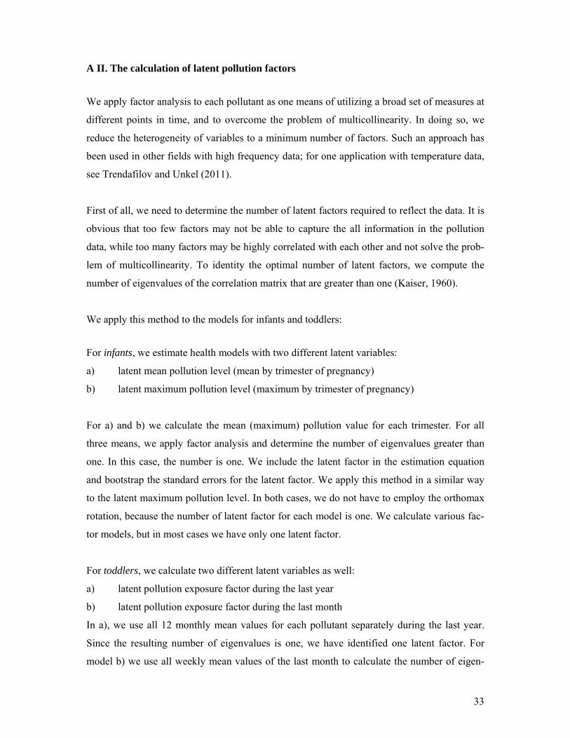
A II. The calculation of latent pollution factors

We apply factor analysis to each pollutant as one means of utilizing a broad set of measures at

different points in time, and to overcome the problem of multicollinearity. In doing so, we

reduce the heterogeneity of variables to a minimum number of factors. Such an approach has

been used in other fields with high frequency data; for one application with temperature data,

see Trendafilov and Unkel (2011).

First of all, we need to determine the number of latent factors required to reflect the data. It is

obvious that too few factors may not be able to capture the all information in the pollution

data, while too many factors may be highly correlated with each other and not solve the prob-

lem of multicollinearity. To identity the optimal number of latent factors, we compute the

number of eigenvalues of the correlation matrix that are greater than one (Kaiser, 1960).

We apply this method to the models for infants and toddlers:

For infants, we estimate health models with two different latent variables:

a) latent mean pollution level (mean by trimester of pregnancy)

b) latent maximum pollution level (maximum by trimester of pregnancy)

For a) and b) we calculate the mean (maximum) pollution value for each trimester. For all

three means, we apply factor analysis and determine the number of eigenvalues greater than

one. In this case, the number is one. We include the latent factor in the estimation equation

and bootstrap the standard errors for the latent factor. We apply this method in a similar way

to the latent maximum pollution level. In both cases, we do not have to employ the orthomax

rotation, because the number of latent factor for each model is one. We calculate various fac-

tor models, but in most cases we have only one latent factor.

For toddlers, we calculate two different latent variables as well:

a) latent pollution exposure factor during the last year

b) latent pollution exposure factor during the last month

In a), we use all 12 monthly mean values for each pollutant separately during the last year.

Since the resulting number of eigenvalues is one, we have identified one latent factor. For

model b) we use all weekly mean values of the last month to calculate the number of eigen-

34

values. Both factors a) and b) are included in our estimation regression and standard errors are

bootstrapped.

35

A III. Other figures and tables Fig. A1: Distance of SOEP households with children to “background” monitors

Note: Location of air monitors in Germany: own calculations.

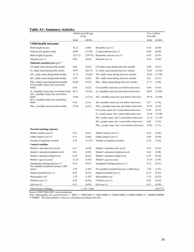
36

Table A1: Summary statistics

Infants up to the age

of one Two- to three-year-olds

mean std.dev. mean std.dev.

Child health outcomes Birth length (in cm) 51.15 (3.06) Bronchitis (yes=1) 0.10 (0.29)

Fetal growth (grams/week) 84.98 (12.98) Croup syndrome (yes=1) 0.08 (0.28)

Birth weight (in grams) 3327.23 (579.97) Respiratory disease (yes=1) 0.14 (0.35)

Disorder (yes=1) 0.06 (0.24) Disorder (yes=1) 0.46 (0.50)

Pollutants (outdoor) (in µg/m3)2

CO (daily mean during birth month) 0.46 (0.25) CO (daily mean during interview month) 0.48 (0.21)

O3 (daily mean during birth month) 45.97 (20.17) O3 (daily mean during interview month) 52.81 (16.24)

NO2 (daily mean during birth month) 31.72 (16.69) NO2 (daily mean during interview month) 30.43 (17.98)

SO2 (daily mean during birth month) 4.70 (2.85) SO2 (daily mean during interview month) 4.61 (2.31)

PM10 (daily mean during birth month) 26.84 (9.25) PM10 (daily mean during interview month) 27.77 (7.80) CO (monthly means last year before birth) 0.46 (0.22) CO (monthly mean last year before interview) 0.46 (0.18)

O3 (monthly means last year before birth) 46.17 (12.62) O3 (monthly mean last year before interview) 48.47 (13.08) NO2 (monthly means last year before birth) 32.06 (15.23) NO2 (monthly mean last year before interview) 29.19 (16.80) SO2 ( monthly means last year before birth) 4.82 (2.41) SO2 (monthly mean last year before interview) 4.27 (1.86)

PM10 (monthly last year before birth) 27.04 (6.35) PM10 (monthly mean last year before interview) 25.39 (5.65)

CO (yearly mean last 3 years before interview) 0.49 (0.19)

O3 (yearly mean last 3 years before interview) 52.54 (13.90)

NO2 (yearly mean last 3 years before interview) 31.14 (13.29)

SO2 (yearly mean last 3 years before interview) 4.92 (1.93)

PM10 (yearly mean last 3 years before interview) 29.56 (7.11)

Parental smoking exposure

Mother smokes (yes=1) 0.21 (0.41) Mother smokes (yes=1) 0.26 (0.44)

Father smokes (yes=1) 0.31 (0.46) Father smokes (yes=1) 0.49 (0.50)

Number of cigarettes smoked 6.39 (11.47) Number of cigarettes smoked 6.20 (9.36)

Control variables

Mother’s education (low level) 0.17 (0.38) Mother’s education (low level) 0.14 (0.35)

Mother’s education (medium level) 0.61 (0.49) Mother’s education (medium level) 0.63 (0.48)

Mother’s education (high level) 0.22 (0.42) Mother’s education (high level) 0.23 (0.42)

Mother’s age (in years) 31.20 (5.44) Mother’s age (in years) 33.34 (3.95)

Immigration background (yes=1) 0.14 (0.35) Immigration background (yes=1) 0.12 (0.32) Net monthly household income (1,000 euros) 2.39 (1.69) Net monthly household income (1,000 euros) 2.50 (1.91)

Single household (yes=1) 0.07 (0.25) Single household (yes=1) 0.15 (0.36)

Municipality size1 3.79 (1.95) Municipality size 1 3.74 (0.32)

Firstborn (yes=1) 0.43 (0.50) Firstborn (yes=1) 0.45 (0.50)

Girl (yes=1) 0.51 (0.50) Girl (yes=1) 0.51 (0.50)

Observations (siblings) 1, 155- 1,268 629-775

Source: SOEP 2002-2007: own calculations. Note: 1Municipality size varies between 1 < 2000; 2 = 2000-5000; 3= 5000-20000; 4= 20000-50000; 5=50000-100000; 6 = 1000000-500000; 7>500000. 2All mean pollution values are calculated according to the EoL.

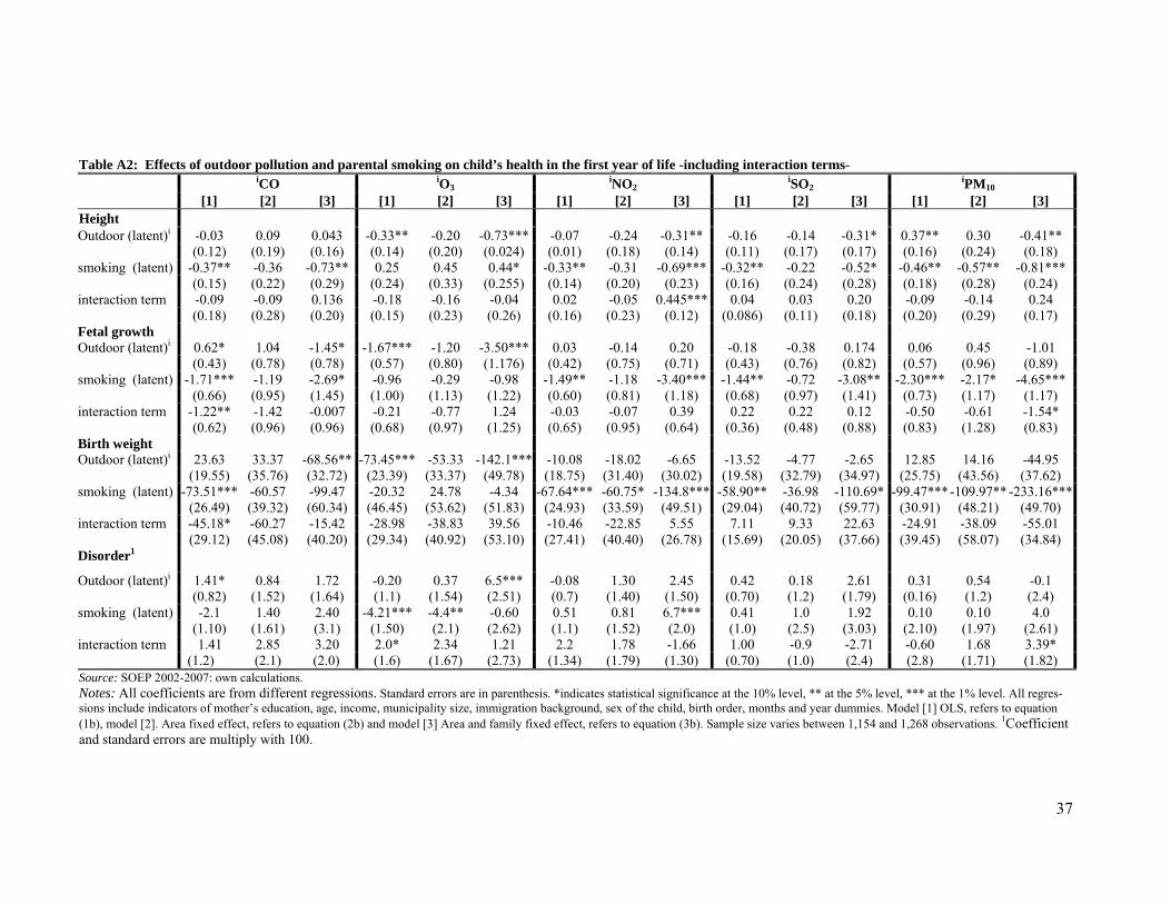
37

Table A2: Effects of outdoor pollution and parental smoking on child’s health in the first year of life -including interaction terms- iCO iO3 iNO2 iSO2 iPM10 [1] [2] [3] [1] [2] [3] [1] [2] [3] [1] [2] [3] [1] [2] [3] Height Outdoor (latent)i -0.03 0.09 0.043 -0.33** -0.20 -0.73*** -0.07 -0.24 -0.31** -0.16 -0.14 -0.31* 0.37** 0.30 -0.41** (0.12) (0.19) (0.16) (0.14) (0.20) (0.024) (0.01) (0.18) (0.14) (0.11) (0.17) (0.17) (0.16) (0.24) (0.18) smoking (latent) -0.37** -0.36 -0.73** 0.25 0.45 0.44* -0.33** -0.31 -0.69*** -0.32** -0.22 -0.52* -0.46** -0.57** -0.81*** (0.15) (0.22) (0.29) (0.24) (0.33) (0.255) (0.14) (0.20) (0.23) (0.16) (0.24) (0.28) (0.18) (0.28) (0.24) interaction term -0.09 -0.09 0.136 -0.18 -0.16 -0.04 0.02 -0.05 0.445*** 0.04 0.03 0.20 -0.09 -0.14 0.24 (0.18) (0.28) (0.20) (0.15) (0.23) (0.26) (0.16) (0.23) (0.12) (0.086) (0.11) (0.18) (0.20) (0.29) (0.17) Fetal growth Outdoor (latent)i 0.62* 1.04 -1.45* -1.67*** -1.20 -3.50*** 0.03 -0.14 0.20 -0.18 -0.38 0.174 0.06 0.45 -1.01 (0.43) (0.78) (0.78) (0.57) (0.80) (1.176) (0.42) (0.75) (0.71) (0.43) (0.76) (0.82) (0.57) (0.96) (0.89) smoking (latent) -1.71*** -1.19 -2.69* -0.96 -0.29 -0.98 -1.49** -1.18 -3.40*** -1.44** -0.72 -3.08** -2.30*** -2.17* -4.65*** (0.66) (0.95) (1.45) (1.00) (1.13) (1.22) (0.60) (0.81) (1.18) (0.68) (0.97) (1.41) (0.73) (1.17) (1.17) interaction term -1.22** -1.42 -0.007 -0.21 -0.77 1.24 -0.03 -0.07 0.39 0.22 0.22 0.12 -0.50 -0.61 -1.54* (0.62) (0.96) (0.96) (0.68) (0.97) (1.25) (0.65) (0.95) (0.64) (0.36) (0.48) (0.88) (0.83) (1.28) (0.83) Birth weight Outdoor (latent)i 23.63 33.37 -68.56** -73.45*** -53.33 -142.1*** -10.08 -18.02 -6.65 -13.52 -4.77 -2.65 12.85 14.16 -44.95 (19.55) (35.76) (32.72) (23.39) (33.37) (49.78) (18.75) (31.40) (30.02) (19.58) (32.79) (34.97) (25.75) (43.56) (37.62) smoking (latent) -73.51*** -60.57 -99.47 -20.32 24.78 -4.34 -67.64*** -60.75* -134.8*** -58.90** -36.98 -110.69* -99.47***-109.97** -233.16*** (26.49) (39.32) (60.34) (46.45) (53.62) (51.83) (24.93) (33.59) (49.51) (29.04) (40.72) (59.77) (30.91) (48.21) (49.70) interaction term -45.18* -60.27 -15.42 -28.98 -38.83 39.56 -10.46 -22.85 5.55 7.11 9.33 22.63 -24.91 -38.09 -55.01 (29.12) (45.08) (40.20) (29.34) (40.92) (53.10) (27.41) (40.40) (26.78) (15.69) (20.05) (37.66) (39.45) (58.07) (34.84) Disorder1

Outdoor (latent)i 1.41* 0.84 1.72 -0.20 0.37 6.5*** -0.08 1.30 2.45 0.42 0.18 2.61 0.31 0.54 -0.1 (0.82) (1.52) (1.64) (1.1) (1.54) (2.51) (0.7) (1.40) (1.50) (0.70) (1.2) (1.79) (0.16) (1.2) (2.4) smoking (latent) -2.1 1.40 2.40 -4.21*** -4.4** -0.60 0.51 0.81 6.7*** 0.41 1.0 1.92 0.10 0.10 4.0 (1.10) (1.61) (3.1) (1.50) (2.1) (2.62) (1.1) (1.52) (2.0) (1.0) (2.5) (3.03) (2.10) (1.97) (2.61)interaction term 1.41

(1.2) 2.85 3.20 2.0*

(1.6) 2.34

(1.67) 1.21

(2.73) 2.2

(1.34) 1.78

(1.79) -1.66 (1.30)

1.00 (0.70)

-0.9 (1.0)

-2.71 (2.4)

-0.60 (2.8)

1.68 (1.71)

3.39* (1.82) (2.1) (2.0)

Source: SOEP 2002-2007: own calculations. Notes: All coefficients are from different regressions. Standard errors are in parenthesis. *indicates statistical significance at the 10% level, ** at the 5% level, *** at the 1% level. All regres-sions include indicators of mother’s education, age, income, municipality size, immigration background, sex of the child, birth order, months and year dummies. Model [1] OLS, refers to equation (1b), model [2]. Area fixed effect, refers to equation (2b) and model [3] Area and family fixed effect, refers to equation (3b). Sample size varies between 1,154 and 1,268 observations. 1Coefficient and standard errors are multiply with 100.

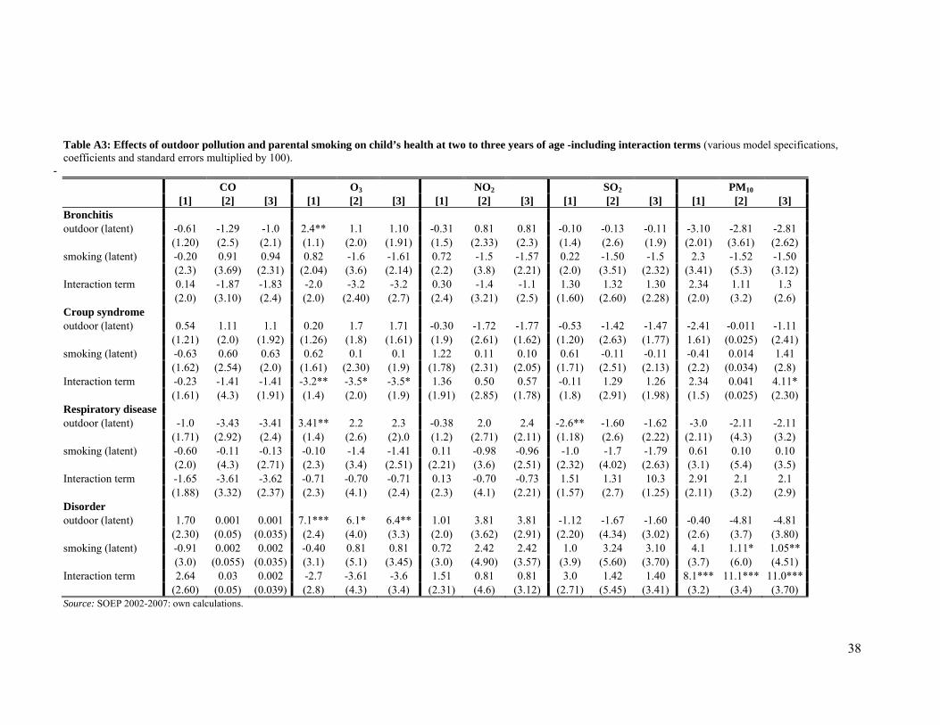
38

Table A3: Effects of outdoor pollution and parental smoking on child’s health at two to three years of age -including interaction terms (various model specifications, coefficients and standard errors multiplied by 100).

-

CO O3 NO2 SO2 PM10 [1] [2] [3] [1] [2] [3] [1] [2] [3] [1] [2] [3] [1] [2] [3]

Bronchitis outdoor (latent) -0.61 -1.29 -1.0 2.4** 1.1 1.10 -0.31 0.81 0.81 -0.10 -0.13 -0.11 -3.10 -2.81 -2.81 (1.20) (2.5) (2.1) (1.1) (2.0) (1.91) (1.5) (2.33) (2.3) (1.4) (2.6) (1.9) (2.01) (3.61) (2.62) smoking (latent) -0.20 0.91 0.94 0.82 -1.6 -1.61 0.72 -1.5 -1.57 0.22 -1.50 -1.5 2.3 -1.52 -1.50 (2.3) (3.69) (2.31) (2.04) (3.6) (2.14) (2.2) (3.8) (2.21) (2.0) (3.51) (2.32) (3.41) (5.3) (3.12) Interaction term 0.14 -1.87 -1.83 -2.0 -3.2 -3.2 0.30 -1.4 -1.1 1.30 1.32 1.30 2.34 1.11 1.3 (2.0) (3.10) (2.4) (2.0) (2.40) (2.7) (2.4) (3.21) (2.5) (1.60) (2.60) (2.28) (2.0) (3.2) (2.6) Croup syndrome outdoor (latent) 0.54 1.11 1.1 0.20 1.7 1.71 -0.30 -1.72 -1.77 -0.53 -1.42 -1.47 -2.41 -0.011 -1.11 (1.21) (2.0) (1.92) (1.26) (1.8) (1.61) (1.9) (2.61) (1.62) (1.20) (2.63) (1.77) 1.61) (0.025) (2.41) smoking (latent) -0.63 0.60 0.63 0.62 0.1 0.1 1.22 0.11 0.10 0.61 -0.11 -0.11 -0.41 0.014 1.41 (1.62) (2.54) (2.0) (1.61) (2.30) (1.9) (1.78) (2.31) (2.05) (1.71) (2.51) (2.13) (2.2) (0.034) (2.8) Interaction term -0.23 -1.41 -1.41 -3.2** -3.5* -3.5* 1.36 0.50 0.57 -0.11 1.29 1.26 2.34 0.041 4.11* (1.61) (4.3) (1.91) (1.4) (2.0) (1.9) (1.91) (2.85) (1.78) (1.8) (2.91) (1.98) (1.5) (0.025) (2.30) Respiratory disease outdoor (latent) -1.0 -3.43 -3.41 3.41** 2.2 2.3 -0.38 2.0 2.4 -2.6** -1.60 -1.62 -3.0 -2.11 -2.11 (1.71) (2.92) (2.4) (1.4) (2.6) (2).0 (1.2) (2.71) (2.11) (1.18) (2.6) (2.22) (2.11) (4.3) (3.2) smoking (latent) -0.60 -0.11 -0.13 -0.10 -1.4 -1.41 0.11 -0.98 -0.96 -1.0 -1.7 -1.79 0.61 0.10 0.10 (2.0) (4.3) (2.71) (2.3) (3.4) (2.51) (2.21) (3.6) (2.51) (2.32) (4.02) (2.63) (3.1) (5.4) (3.5) Interaction term -1.65 -3.61 -3.62 -0.71 -0.70 -0.71 0.13 -0.70 -0.73 1.51 1.31 10.3 2.91 2.1 2.1 (1.88) (3.32) (2.37) (2.3) (4.1) (2.4) (2.3) (4.1) (2.21) (1.57) (2.7) (1.25) (2.11) (3.2) (2.9) Disorder outdoor (latent) 1.70 0.001 0.001 7.1*** 6.1* 6.4** 1.01 3.81 3.81 -1.12 -1.67 -1.60 -0.40 -4.81 -4.81 (2.30) (0.05) (0.035) (2.4) (4.0) (3.3) (2.0) (3.62) (2.91) (2.20) (4.34) (3.02) (2.6) (3.7) (3.80) smoking (latent) -0.91 0.002 0.002 -0.40 0.81 0.81 0.72 2.42 2.42 1.0 3.24 3.10 4.1 1.11* 1.05** (3.0) (0.055) (0.035) (3.1) (5.1) (3.45) (3.0) (4.90) (3.57) (3.9) (5.60) (3.70) (3.7) (6.0) (4.51) Interaction term 2.64 0.03 0.002 -2.7 -3.61 -3.6 1.51 0.81 0.81 3.0 1.42 1.40 8.1*** 11.1*** 11.0*** (2.60) (0.05) (0.039) (2.8) (4.3) (3.4) (2.31) (4.6) (3.12) (2.71) (5.45) (3.41) (3.2) (3.4) (3.70) Source: SOEP 2002-2007: own calculations.

39

Notes: All coefficients are from different regressions. Standard errors are in parenthesis. *indicates statistical significance at the 10% level, ** at the 5% level, *** at the 1% level. All regres-sions include indicators of mother’s education, age, income, municipality size, immigration background, sex of the child, birth order, child’s age in months, month and year dummies. Model [1] OLS, refers to equation (1b), model [2] Area fixed effect, refers to equation (2b) and model [3] Area and family fixed effect, refers to equation (3b). Sample size varies between 629 and 775 obser-vations. Equation (1c) and model [2] refer to equation (3c). Sample size varies between 629 and 775 observations.