Political versus Economic Institutions

in the Growth Process∗

Emmanuel FlachaireAix-Marseille University†

Cecilia Garcıa-PenalosaAix-Marseille University‡

Maty KonteAix-Marseille University§

September 2011

Abstract

After a decade of research on the relationship between institutions and growth, there isno consensus about the exact way in which these two variables interact. In this paper were-examine the role that institutions play in the growth process using data for developed anddeveloping economies over the period 1970-2000. Our results indicate that the data is bestdescribed by an econometric model with two growth regimes. Political institutions are thekey determinant of which regime an economy belongs to, while economic institutions havea direct impact on growth rates within each regime. These findings support the hierarchyof institutions hypothesis, whereby political institutions set the stage in which economicinstitutions and policies operate.

JEL Classification: O43 - O47

Key words: growth, institutions, mixture regressions

∗Ackowledgements: We would like to thank Ann Owen for providing some of the data used in this paper, aswell as Theo Eicher, Michel Lubrano and seminar participants at Greqam. Garcıa-Penalosa is a CNRS researcherat Greqam and her work was partly supported by the French National Research Agency Grant ANR-08-BLAN-0245-01.†GREQAM, Centre de la Vieille Charite, 2 rue de la Charite, 13002 Marseille - Email :

emmanuel.flachaire@univ-cezanne.fr‡GREQAM, Centre de la Vieille Charite, 2 rue de la Charite, 13002 Marseille - Email : cecilia.garcia-

penalosa@univmed.fr§GREQAM, Centre de la Vieille Charite, 2 rue de la Charite, 13002 Marseille - Email : maty.konte@etu.univ-

cezanne.fr

1

1 Introduction

Over the last decade a heated debate has taken place over the role of institutions for economic

growth. Although simple correlations indicate that growth and institutional quality are closely

related, there is no consensus about the exact way in which these two variables interact. On the

one hand, the evidence on cross-country income gaps has found that income levels are strongly

correlated with economic institutions, while political institutions have been argued to be ‘deep’

causes of development, acting through their impact on policies and economic institutions. On

the other, studies of the determinants of growth rates have focused on the role of political

institutions, particularly that of democracy, and find that while the level of institutional quality

has no impact on growth rates, changes in the political framework do.1 In this paper we

reconsider the relationship between institutions and growth and argue that both political and

economic institutions are crucial determinants of growth rates albeit in very different ways.

The motivation for our approach is the hierarchy of institutions hypothesis proposed by

Acemoglu et al. (2005), which argues that political institutions ‘set the stage’ in which economic

institutions can be devised and economic policies implemented. As such, their role is indirect and

may operate either through their impact on the economic institutions and policies that a country

chooses or through the effect that these have on growth. While there is some evidence for the

former,2 little work has been done on the latter. We hence focus on the second mechanism and

argue that while economic institutions affect growth rates in the same way as standard variables

such as investment or education, political institutions are one of the deep causes of growth.3

To test this hypothesis we follow recent work which emphasizes the existence of different

growth regimes such that standard growth determinants have different marginal effects on growth

across regimes.4 Our approach consists in using a finite mixture of regression models, a semi-

parametric method for modeling unobserved heterogeneity in the population that allows us to

relax the hypothesis of one growth model. In contrast to other approaches that divide the data

into groups, mixture regressions let the data determine the variables that determine group mem-

bership and countries are endogenously allocated to a group, implying a much greater flexibility

and better fit of the data than earlier work on parameter heterogeneity. This framework allows

us to test whether political institutions rather than having a direct impact, determine which

1See, amongst others, Hall and Jones (1999), Acemoglu et al. (2001) and Easterly and Levine (2003) on theimpact of institutions on development and Barro (1996), Persson (2004) and Persson and Tabellini (2006) on theeffect of democracy on growth rates.

2See, for example, Persson (2004) and Eicher and Leukert (2009).3See Galor (2005) for a discussion of deep and proximate causes of growth.4See Owen et al. (2009), Vaio and Enflo (2011) and Bos et al. (2010).

2

regime a country belongs to.

We estimate mixture regressions on a panel of developed and developing countries over the

period 1970-2000. Our results indicate that the data is best described by a two-regime model,

with roughly a third of countries in a high-growth group and the rest in a group with lower but

more dispersed growth rates. Political and economic institutions play very different roles. The

former are the key determinant of regime membership, while economic institutions are impor-

tant in determining growth rates within each of the two regimes, supporting the hierarchy of

institutions hypothesis. The impact of economic institutions on growth is substantial, although

its magnitude differs across groups. In the high-growth group, an increase of one standard devi-

ation of the economic institutions index results in an increase in growth of 0.4 percentage points,

while in the low-growth group the same increase raises growth by a full percentage point. Our

results hence suggest that when political institutions are weak, growth is more sensitive to the

choice of economic institutions than when the former are strong.

The paper contributes to the literature on the relationship between growth and institutions,

dating back to the work of North (see North 1981). Most empirical analyses linking institutions

and growth rates have focused on the effect of the degree of democratization, yet the evidence for

a significant effect is weak; see Barro (1996). Recent work, such as Persson and Tabellini (2006),

Persson and Tabellini (2008), Rodrik and Wacziarg (2005) and Nannicini and Ricciuti (2010),

has found that it is not being a democracy but rather becoming one what matters for growth.

For example, Persson and Tabellini (2008) find that the transition from autocracy to democracy

increases a country’s annual growth rate by 1 percentage point. Moreover, Persson and Tabellini

(2006) maintain that the difficulty in identifying the impact of political regimes from within-

country variations is that democracy is too broad a concept. They focus on three specific

situations in which democratic reform impacts growth: the correlation between democratizations

and economic liberalizations, instances where democratic institutions influence fiscal and trade

policies, and allowing for ‘expected political reforms’ that anticipate actual reforms, and in all

these cases they find a stronger growth effect of democracy than is obtained in more standard

growth regressions.5 Our approach is complementary to these studies in two aspects. On the

one hand, our aim is to find a role for the level of political institutions in the growth process,

rather than for changes. On the other, we postulate that their impact is not a direct one but

rather operates indirectly as they determine to which growth regime a country belongs to.

5Some of this work has also considered the question of parameter heterogeneity when examining the impactof transitions in and out of democracy on growth rates. Persson and Tabellini (2008) and Nannicini and Ricciuti(2010) examine the different impact of transitions into and out of democracy.

3

Our work is also related to empirical analyses of the effect of institutions on cross-country

income differences, such as Knack and Keefer (1995), Hall and Jones (1999) and Acemoglu et al.

(2001). Although methodologically different, this literature is asking conceptually similar ques-

tions. Most studies have found that economic institutions are strongly correlated with the level

of development, while political institutions tend to be insignificant in cross-country regressions.6

As a response, Acemoglu et al. (2005) have argued that different types of institutions act at

different levels, with political institutions being part of the deep causes of development, while

economic institutions belong to the set of proximate causes. Eicher and Leukert (2009) find

support for this hypothesis when they use political institutions as an instrument for economic

institutions, which in turn have a significant effect on output levels. Similarly, the literature

on the determinants of growth rates has compared the impact of the two sets of institutions,

and arrived to similar conclusions. Glaeser et al. (2004) highlight the fact that, when con-

trolling for education, the level of economic institutions has a significant coefficient in growth

regressions while political institutions do not. Giavazzi and Tabellini (2005) find that economic

liberalizations foster growth, and this effect is magnified if they are accompanied by political

liberalizations.

Methodologically, the paper builds on the extensive literature on growth regimes, starting

with Durlauf and Johnson (1995).7 Some recent papers have proposed the use of mixture

regressions models to identify different growth regimes. Vaio and Enflo (2011) use historical

data to identify the role of trade openness, while Bos et al. (2010) examine whether, in a world

with different growth regimes, countries change regime over time. Neither of these analyses

considers the role of institutions. Owen et al. (2009) allow for the possibility that institutions

affect group membership, and some of our results will revisit their empirical analysis. The

crucial difference with their work is that we allow institutions to have both a direct and an

indirect impact on growth, and in doing so find that economic and political institutions play

very different roles.

The paper is organized as follows. Section 2 discusses the role of institutions in the growth

process, while section 3 describes the data, focusing on the measurement of institutions and the

correlation between political and economic institutions. In section 4 we use standard regressions

methods all of which indicate that although economic institutions have a positive and significant

effect on growth, political institutions play no role. We then move onto the central analysis of

6See also Acemoglu et al. (2002), Easterly and Levine (2003), Dollar and Kraay (2003), Glaeser et al. (2004),Acemoglu et al. (2005), and Glaeser et al. (2007).

7See also Brock and Durlauf (2001) and Eicher et al. (2007), amongst others.

4

the paper, with section 5 testing the hypothesis that political institutions determine to which

regime a country belongs to and section 6 performing a number of robustness analyses. The last

section concludes.

2 Institutions in the growth process

Our estimations will be based on the following growth regression model:

growth = δ0 + δ1 log(gdp0) + δ2 log(pop) + δ3 log(inv) + δ4 log(educ0)

+ δ5eco + δ6dem + ε.(1)

The dependent variable is the average annual growth rate of real per capita GDP (growth), and

the core covariates are initial GDP per capita (gdp0), the average annual population growth rate

(pop), the average investment to output ratio (inv) and initial years of schooling of the labor

force (educ0). The standard approach is to also add a term that captures the rate of growth of

total factor productivity (TFP) which, in a Solow-type world, would be exogenous and common

to all countries.

Alternatively, we can think of TFP growth as varying across countries and overtime, accord-

ing to some country specific variables. Equation 1 postulates that TFP growth is driven by the

institutional framework of the economy as captured by measures of economic institutions (eco)

and of political institutions (dem). As discussed earlier, starting with Barro (1996) and Hall and

Jones (1999), institutions have been argued to have a direct effect on growth and productivity.

In recent years a number of theoretical arguments have been put forward to support this rela-

tionship. For example, Aghion et al. (2008) maintain that political and economic freedoms are

correlated with freedom of entry in product markets, which in turn encourages innovation. More

generally, the entire literature on R&D-driven endogenous growth relies on the existence of high

quality economic institutions such as free markets, the protection of property rights -particularly

intellectual property rights- , and individual freedom to move across sectors or occupations.8

Our prior, in the light of this literature, is that economic institutions are a key factor determin-

ing productivity growth. Arguments for a direct impact of political institutions on productivity

growth have also been put forward, such as those in Aghion et al. (2008) or Acemoglu (2008),

who maintains that democracies may be better able to take advantage of new technologies. Yet

these authors also argue that in the early stages of development autocracies may result in faster

growth,9 introducing ambiguities on the relationship between political institutions and growth.

8The role of intellectual property right protection has received substantial attention in the literature, see forexample Eicher et al. (2006), while that of credit markets or limits to product market entry have been exploredby Aghion et al. (2005) and Aghion et al. (2008), respectively.

9See also D. Acemoglu and Zilibotti (2006).

5

It is also possible that, as emphasized by the hierarchy of institutions hypothesis, the impact

of political constraints is not direct but rather determines the coefficients on the covariates in

1. This idea has been recently formalized by Larsson and Parente (2011) who model the way

in which democratic and autocratic regimes choose policies and their impact on growth. They

maintain that all democracies implement similar policies, chosen by voters, which are conducive

to moderate growth. In contrast, autocrats choose policies according to their own preferences

which are heterogeneous across regimes. Some autocrats impose policies that are conducive to

fast growth even if this entails costs for some sectors of the electorate, while others prefer to

dampen growth in order to benefit minority groups. As a result, the average performance of

democratic and non-democratic regimes may not be very different, but the variance of growth

rates would be much larger in the latter.

In order to test this hypothesis, we will consider the possibility that political institutions

determine the type of growth-regime a country belongs to. Our expectation is that democratic

countries exhibit rather homogeneous growth rates while non-democratic ones are in a regime

where growth is highly sensitive to policy choices. In particular, we will examine whether in

non-democratic regimes the economic institutions imposed by the government become a mayor

factor determining growth.

3 The data

Most of the data we employ has been extensively used by the empirical literature on the determi-

nants of growth rates. We use a panel comprising 74 developed and developing countries for the

period 1970-2000. The data were provided by Ann Owen and were used in Owen et al. (2009).

Observations are averaged over 5-year periods, yielding (at best) six data points per country

and totaling 406 observations. Table 7 presents descriptive statistics and the data sources. Ob-

viously, the descriptive statistics for the panel are similar to those reported in Table 1 of Owen

et al. (2009), except for our measures of institutions which differ from theirs.

Owen et al. use as measures of economic and political institutions ‘law and order’ and

‘democracy’ obtained from the International Country Risk Guide (ICRG), both of which have

been widely used in the literature on cross-country growth differences, starting with Knack

and Keefer (1995) and Mauro (1995). These measures have been criticized by Glaeser et al.

(2004) as they tend to reflect outcomes rather than political constraints. A more satisfactory

variable is that provided by Polity IV, and constructed by political scientists, which aims directly

at measuring political constraints. From our perspective, the ICRG variables also have the

6

drawback that they start only in the mid 1980s, i.e. half-way through our period of analysis.

This is not a problem for Owen et al. (2009) since they focus on the role of institutions as

determinants of growth regimes and hence use only one time-invariant observation per country.

In contrast, we will allow institutions to appear both as determinants of the regime and as

standard covariates in the panel analysis, hence requiring a time dimension. We therefore use

Polity IV and Fraser Institute indices, both of which are available for the entire period that we

consider.10

We measure economic institutions by the index of Economic Freedom of the World (EFW)

from the Fraser Institute. Economic freedom measures the extent to which property rights

are protected and the freedom that individuals have to engage in voluntary transactions. This

measure takes into account the respect of personal choices, the voluntary exchange coordinated

by markets, freedom to enter and compete in markets, and protection of persons and their

property from aggression by others. The index is an unweighted average of 5 elements: the size

of the government in the economy, the legal structure, security of property rights, the access

to sound money, the freedom to trade internationally, and the regulation of credit, labor and

business. The country with the lowest value in our sample is Guinea Bissau (3.69) and the one

with the largest is Singapore (7.79). Our main measure of political institutions is the degree

of democracy obtained from Polity IV. This measure takes into account the competitiveness of

executive recruitment, the openness of executive recruitment, the constraints on the executive,

and the competitiveness of political participation. It ranges between 0 and 10, with a value of 0

denoting an autocratic government and a value of 10 full democracy. In our analysis below, we

will allow institutions to play different roles, as they can have a direct impact on the growth rate

or affect the environment in which growth occurs. Hence we define as dem5 and eco5 the 5-year

averages of our measures of political and economic institutions, respectively, and as dem30 and

eco30 the averages over the entire period.

The correlation matrix in Table 2 presents some well-established facts. First, the two mea-

sures of institutions are only moderately correlated (see Glaeser et al. 2004). Second, the

correlation between growth and institutions is stronger in the case of economic institutions than

political ones, which exhibit a correlation of only 0.08 compared to 0.29 for economic institu-

tions. Lastly, democracy covaries with both education and latitude, raising the question of to

what extent these three variables have independent explanatory power in growth regressions.

To further understand the differences between our two institutional variables, Table 3 de-

10For further discussion of the measurement of institutions see Haan (2003) and Glaeser et al. (2004).

7

composes the data into their between-country and within-country components. We can see that

the two variables have roughly the same mean but the dispersion of dem5 is substantially greater

than that of eco5. The within country component is smaller than the between-country one in

both cases, but the difference between the two is much larger for dem5, indicating the greater

relative stability of this measure. Figure 1 gives some country examples of the evolution of the

two variables over time, with democracy being depicted by the continuous line and economic

institutions by the dashed one. The figure indicates substantial variations over time as well

as very different country patterns. In some cases, such as Botswana, the two institutions are

virtually identical, but for most countries this is not the case. There are many instances in

which there is a gap between the two variables, but the time trend is the same for both (France,

Tunisia, Venezuela). The size of the gap varies, being small in France and large in Tunisia,

where economic institutions are much better than political ones. In the US and in China po-

litical institutions have remained stable while economic ones have improved over time, but the

difference between the two countries is that in the former eco5 has been catching up with dem5,

while in the latter the two measures have diverged over time. The overall tendency has been for

an improvement in institutional quality but there are exceptions, with Brazil, Peru, Sri Lanka,

Venezuela and Zimbabwe exhibiting a deterioration of one or the other measure.

4 Standard regression models

The data discussed above indicates that our two measures of institutions are not only conceptu-

ally different, but also diverse in terms of their evolution over time and the degree of correlation

with economic performance, raising the question of whether their role in the growth process is

also different. In order to address this question, we start by considering the standard approaches

that have been used to examine the determinants of growth rates, and ask to what extent these

are able to satisfactorily identify the impact of institutions. We first run cross-section regres-

sions, using Ordinary Least Squares (OLS) and Instrumental Variables (IV) estimation methods.

Then, we consider panel data, using Fixed-Effect (FE) and Random-Effects (RE) models, and

show that a similar pattern emerges from all the estimated models.

4.1 Cross-section

We start by looking only at the cross-sectional dimension of the data, averaging variables for the

entire 30-year period. The cross-section includes only 73 countries, since Guinea-Bissau does

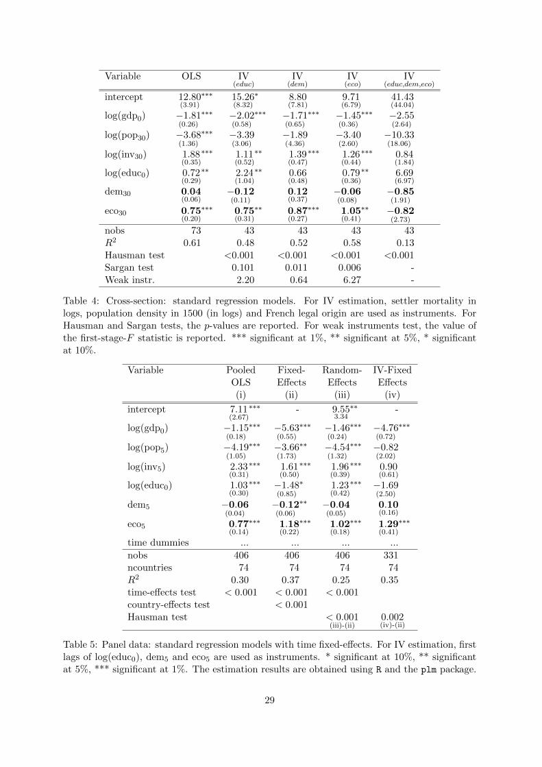
not have data on education at the beginning of the period. The first column in Table 4 presents

8

OLS estimation results for the cross-section. The coefficient on initial GDP (gdp0) is significant

and negative in line with the convergence hypothesis. The coefficients on education (educ0),

investment (inv) and economic institutions (eco) are all significant and have a positive impact

on growth, while the coefficient on the population growth rate (pop) is significant and negative.

In contrast, political institutions (dem) exhibits an insignificant coefficient.

The literature has extensively discussed the fact that both institutional quality and edu-

cational attainment may be determined by economic performance. To deal with the possible

endogeneity of these variables, we use IV estimation with settler mortality (in logs), population

density in 1500 (in logs) and a dummy variable for French legal origin as instruments.11 Columns

(ii) to (v) in table 4 present IV estimation results with, respectively, education, political insti-

tutions, economic institutions, and the three variables together taken as endogenous. When

we treat only one variable as endogenous (educ, dem or eco), we can see that the coefficient of

economic institutions is always significant at the 5% level, while political institutions still have

no effect on growth. Moreover, we can see that the null hypothesis of consistent OLS estimation

is always rejected (Hausman test), and that the validity of the instruments is rejected when educ

is endogenous (Sargan test), while the null of weak instruments is never rejected.12 The validity

of the instruments when we allow for the endogeneity of institutions is an important question:

this hypothesis is rejected at 5% when eco and dem are endogenous. Furthermore, having weak

instruments is problematic since it can lead to biased estimates and poor finite sample inference

(see Stock et al. 2002). Our results suggest that the choice of appropriate instruments for

institutions is a difficult issue, as pointed out by a number of authors (see Durlauf et al. 2005,

and Pande and Udry 2006). Note that, when we consider the three variables as being simulta-

neously endogenous (last column) the standard errors in parenthesis increase dramatically and

none of their coefficients is significantly different from zero. This lack of precision maybe due to

the small number of observations in the sample together with the large number of parameters

to estimate. Since our choice of instruments implies that observations are available only for

countries with a colonial history, the sample size is very small -only 43 observations- and the

estimation and test can suffer from small sample problems.

Our negative results on the validity and weakness of the instruments together with the small

number of observations suggest that IV estimation results are not satisfactory in our cross-

section analysis. It is then possible that the difficulty in identifying the effect of institutions,

11See Acemoglu et al. (2005) for a discussion of these instruments.12The test statistic is the first-stage F -test in the case of one endogenous variable. Instruments are supposed

to be strong if it is greater than 10, and weak otherwise.

9

particularly of political institutions, is due to these problems. The usual way to increase the

precision of the estimation and get more reliable results is to use more observations. Since in

growth regressions we have a limited number of countries, the only option is to use panel data.

4.2 Panel

The first column in table 5 presents pooled OLS estimation results using our panel data set. We

include time dummies in the covariates to take into account time-effects. Standard errors are

smaller than those of the cross-sectional OLS estimation (Table 4, column 1) and, as expected,

the coefficient estimates are more precise. We can see that economic institutions still have a

significant and positive coefficient, while that on political institutions remains insignificant.

However, using pooled OLS estimation does not make use of the most important advantage

of using panel data. If key variables are unobserved, coefficient estimates can be significantly

biased. IV estimation can be used to solve this problem of omitted variable bias but, as we saw

above, it is difficult to find good instruments. Panel estimation is an alternative approach to solve

this problem, using the time dimension to control for unobserved but fixed omitted variables.

A frequent way of considering individual unobserved heterogeneity is to allow the intercept in

model (1) to be different for every country, δ0i, while the other coefficients are assumed to be the

same across countries, δ1, . . . , δ7. We can define δ0i including in the regression a dummy for each

country (fixed-effects) or modelling it as a random coefficient drawn from a normal distribution

(random-effects). The second and third columns in Table 5 present estimation results for fixed-

effects and random-effect models, with time dummies in the covariates (models (ii) and (iii)).

Again, we can see that economic institutions have significant and positive coefficients, while

those on political institutions tend not to be significant. For the fixed-effects model, the test of

the null that the country fixed-effects are constant is rejected (country-effects test with p-value

< 0.001), which suggests that the pooled OLS estimation is inappropriate, while the Hausman

test suggests that the random-effects model is less appropriate than the fixed-effects one.

The last column in Table 5 presents estimation results for fixed-effects models with the IV

estimator used by Balestra and Varadharajan-Krishnakumar (1987). We use the first lags of

education and institutional variables as instruments and find that the conclusions on the role

of economic and political institutions remain unchanged: coefficient estimates are significant for

eco, not for dem.

10

4.3 Discussion

The results using standard regression models give a consistent picture: economic institutions

have positive and significant coefficients, while those on political institutions are not significant.

Our findings indicate that not including economic institutions in growth regressions may lead

to omitted variable biases on the other coefficients. As for the role of political institutions, one

possible interpretation is that the degree of democracy has no impact on growth. An alternative

is that the implicit assumptions imposed by the standard approach are too constraining and do

not allow the identification of the impact of this type of institutions. In particular, we have been

estimating regressions models in which all countries follow the same growth process. But what

if they do not?

Both Acemoglu et al. (2005) and Persson (2004) have argued that political institutions set

the stage for economic activity and the creation of economic institutions. It is hence possible

that political institutions do not affect growth rates per se but rather the way in which different

covariates impact growth. That is, they could be a determinant of the type of growth regime

in which a country finds itself. To investigate this hypothesis, we need to go beyond standard

regression models. Our proposed approach is to use finite mixture of regression models.

5 Finite-mixture models

5.1 Method

Finite mixture of regression models are semiparametric methods for modeling unobserved het-

erogeneity in the population. They allow us to relax the hypothesis of one growth model and to

assume that there may exist several growth paths, that is, different groups such that the growth

determinants may have different marginal effects across groups. In the regression model (1), this

is equivalent to relaxing the hypothesis that the coefficients δ1, δ2, δ3, δ4, δ5 and δ6 are common

to all countries. To illustrate the approach, let us consider the simple case of two groups, or

two growth paths. A mixture of linear regressions assumes that an observation belonging to

the first group and one belonging to the second group would not be generated by the same

data-generating process. The mixture model can be written as follows:

Group 1: y = xβ1 + ε1, ε1 ∼ N(0, σ21),

Group 2: y = xβ2 + ε2, ε2 ∼ N(0, σ22),(2)

where y is the dependent variable, x a set of covariates, and ε1 and ε2 are independent and

identical normally distributed error terms within each group, with variances of σ21 and σ22,

respectively. Since the sets of coefficients β1 and β2 are not (necessarily) equal, covariates x do

11

not explain in the same way differences in y between observations belonging to the first group

and between observations belonging to the second group. Applied to our growth regression

model, this mixture model assumes that countries can be classified into two groups, associated

to two different growth paths, and at least one covariate does not explain identically growth

discrepancies within the two groups. Note that such assumption can be taken into account in

the standard regression model (1) if we include additional covariates computed as cross-products

of the variables of interest with a dummy variable that specifies group membership. However, in

this case the groups have to be defined a priori according to some prior believe of the researcher,

such as the hypothesis that the convergence coefficient is different for OECD countries than for

other economies. In contrast, in a finite-mixture model, group membership is not imposed

but rather estimated so as to create classes that are homogeneous in terms of the relationship

between y and x. Moreover, the number of groups is not fixed but endogenously determined

according to an econometric criterion or test.

A set of additional covariates, called concomitant variables, can be used to characterize

group profiles. Concomitant variables play the same role as covariates in a multinomial re-

gression model designed to explain group membership. The roles of standard covariates and of

concomitant variables are different: standard covariates help to explain variations within groups,

whereas concomitant variables explain variations between groups. As a result the values of the

concomitant variables will determine the probability that a particular country belongs to one

class or another.

A general mixture regression model can be written as follows:

f(y|x, z,Θ) =K∑k=1

πk(z, αk)fk(y|x ;βk, σk), (3)

where K is the number of components or groups, πk(z, αk) is the probability of belonging

to group k with a set of specific concomitant variables z, and fk(y |x;βk, σk) is a conditional

probability distribution characterized by a set of parameter and of covariates x. The parameters

αk, βk and σk are unknown and hence estimated. If we consider fk as Gaussian distributions

with conditional expectations equal to E(y|x) = xβk, for K = 1 this model reduces to (1) and

for K = 2 this model reduces to (2).

For a given number of components K, finite mixture models are often estimated by maximum

likelihood with the EM algorithm of Dempster et al. (1977). The log-likelihood function can

be highly non-linear and a global maximum can be difficult to obtain. It is then recommended

to perform the estimation with many different starting values. The number of components K

can be selected minimizing a criterion, such as the Bayesian Information Criterion, denoted BIC

12

and developed by Schwarz (1978), or the Conditional Akaike Information Criterion (CAIC, see

Sugiura 1978, Hurvich and Tsai 1989, and Burnham and Anderson 2002). More specifically, the

BIC is defined as

BIC = −2ˆ+ (#param) log n (4)

where ˆ is the estimated value of the log-likelihood and n is the number of observations.13 A

similar expression defines the CAIC, which also includes a penalty determined by the effective

degrees of freedom.

Mixture models then have two desirable features. First, covariates are allowed to have

different marginal effects across groups. Second, mixture models have the ability to evaluate

the profile of the different groups, or growth paths, using concomitant variables which need

not necessarily be binary, in contrast with often-used groups such as OECD-membership or

regional dummies. Moreover, the resulting classification is in terms of probabilities, so that

some countries will be part of a group with a high probability but others may have features

that imply a more nuanced position. What the model does not allow is for a country to be in

different groups at different times as the concomitant variables must be constant over time.14

5.2 Empirical results

Our interpretation of the hierarchy of institutions hypothesis is that political institutions do

not have a direct effect on growth but rather determine the growth regime in which a country

finds itself. In contrast, economic institutions are similar to other growth determinants such as

investments in physical or human capital. In order to test this hypothesis, we estimate a mix-

ture model of regressions in which the political institutions variable (dem) acts as concomitant

variable and the economic institutions variable (eco) as a standard covariate.

Table 6 presents estimation results of the mixture model. As in the earlier panel analyses,

our dependent variable is the annual rate of growth averaged over five years. For each five-year

period the standard covariates are averaged over the period, except for initial gdp and initial

education for which we use the first observation. In contrast, political institutions, which act as

concomitant, are averaged over the entire 30-year period since the model does not allow countries

to change regime over time and requires a single observation per country. An alternative would

be to use the initial value, an approach that we have found to give equivalent results.

The results for K = 1 are given in the first column (Pooled) and for K = 2 in columns 2-3 (

13For more details on finite mixture models see McLachlan and Peel (2000) and Ahamada and Flachaire (2010).See also the discussion in Owen et al. (2009).

14The question of regime migration is a complex one and has been recently addressed by Bos et al. (2010).

13

Mixture). The last two columns (Wald test) test the null of equal coefficients in the two groups.

We estimated the mixture model for larger values of K, but the BIC and CAIC criteria were

minimized for K = 2, leading us to select the mixture model with 2 groups (BIC=1847.9). Note

that the value of the BIC for the pooled model is equal to 1921.2, implying that a significant

improvement in fitting the data is obtained with the selected finite-mixture model. There is

also an improvement in the R2, both compared to the pooled regression of Table 6 and to the

fixed effects model of Table 5. The marginal impact of all covariates is not the same within the

groups, clearly indicating that there are two distinct growth processes.

The results imply that both types of institutions affect growth, with the coefficients on eco

and dem being both significant at 1%. Their roles are nevertheless different. Political institu-

tions determine group membership, with the negative coefficient on dem indicating that when

this variable increases, the probability of belonging to the second group decreases. Economic

institutions are, just as in the standard regressions in section 4, a determinant of the growth

rate, with better institutions increasing growth in both groups but having a larger effect in

economies with low levels of democracy. These results support the hypothesis that economic

and political institutions operate at different levels of the growth process.

We can see substantial differences in the determinants of growth rates across the two groups.

The coefficient on initial gdp is larger for group 2, indicating that for these countries (conditional)

catching up is more important than for the high-democracy economies. A possible interpretation

is that group 2 growth rates can be explained by a neoclassical growth model, while in group 1

other mechanisms -such as endogenous technological change- are at play. Investment in physical

capital has a positive and significant coefficient for both groups, while human capital and the

population growth rate present coefficients of opposite signs across groups.15 The impact on eco

is larger for group 2,16 which suggests that, ceteris paribus, an improvement in economic insti-

tutions would have a smaller effect on growth in the high-democracy group than low-democracy

countries. More specifically, an improvement of economic institutions of one standard deviation

would increase the growth rate by 0.36 percentage points for group 1 countries and by almost a

full percentage point (0.96) for those in group 2.

The relative impacts of growth determinants also vary across groups. In the high-democracy

group investment, population growth and economic institutions have roughly similar effects,

with one standard deviation in each of these variables increasing growth by 0.52, 0.41 and 0.36

15On the empirical relationship between growth and human capital see, amongst others, de la Fuente andDomenech (2001) and Temple (2001).

16This is in line with the findings of Eicher and Leukert (2009) who divide their sample between OECD andnon-OECD countries and obtain that economic institutions have a stronger effect on output levels in the latter.

14

percentage points, respectively, while our proxy for human capital -average years of education-

has a negative contribution. In contrast, in low-democracy countries the impact of investment in

physical capital is well above that of other factors. An increase of one standard deviation raises

annual growth by 1.39 percentage points; eco also has a large effect (0.96 percentage points),

while the impact of education is more moderate, with an increase of one standard deviation

adding 0.48 percentage points to growth rates. Faster population growth has a substantial

negative effect, with one standard deviation reducing growth by 0.90 points.

Consider now the composition of the two groups. The probability that a specific country

belongs to a given group can be computed using Bayes rule, with the posterior probability that

country i belongs to group k being equal to

πik =πk(zi, αk)fk(yi|xi ; βk, σk)∑Kk=1 πk(zi, αk)fk(yi|xi ; βk, σk)

(5)

We use the model reported in Table 6 to compute πik, and allocate country i to group 1 if and

only if the probability of being in that group is greater than that of being in group 2. The

first group includes 24 countries and the second 50. Table 7 reports the classification of the

countries with their group membership posterior probability. In general, these probabilities are

close to one, yet there are some exceptions such as Sri Lanka which has a probability of only

0.65 of being in group 1. Most of the countries belonging to the first group are rich countries,

although it also includes Botswana, Egypt, Sri Lanka, and Uganda. In the second group we find

middle- and low-income countries, yet the classification does not exactly coincide with the ones

obtained by ad hoc ex ante divisions. For example, it includes several OECD members (Chile,

Ireland, Mexico, Norway, Poland, and Turkey) and the East-Asian ‘tigers’ (Korea, Malaysia and

Singapore).

The bottom panel of Table 7 reports the average values of growth and institutions for the

two groups, as well as the within-group standard deviations. There are important differences

in some variables but not in others. The average growth rate is 2.287% for the high-democracy

group and only 1.425% for the low-democracy one. However the latter exhibits a much larger

standard deviation (3.238 against 1.558 for the high-democracy group); this is not surprising

given that the group includes both some of the so-called ‘growth miracles’ and ‘growth disasters’;

see Durlauf et al. (2005). The larger coefficients on growth determinants obtained for group 2

help us understand the much larger variance of growth in those countries, since they imply that

a given difference in, say, investment would result in a larger difference in growth performance

in the second group than in the first one. Differences across groups in economic institutions are

small, with average values of 6.483 and 5.459 and similar standard deviations. In contrast, group

15

1 exhibits an average value of our index of political institutions which is more than twice that

observed for group 2 countries (8.929 and 4.247, respectively). Although the standard deviation

of dem is somewhat lower for group 1 than for group 2, it nevertheless indicates a substantial

variation in the quality of political institutions even for this group.

6 Robustness analysis

6.1 The determinants of group membership

In order to test the robustness of our results we conduct a number of further estimations. We

start by considering alternative specifications for the concomitant variables.

Table 8 considers a wide set of concomitant variables that includes both political and eco-

nomic institutions, as well as education, OECD membership and geographical characteristics.

There are two reasons for including education. First, some of the early literature on multiple

growth paths postulated that education levels were a key determinant of which group a country

belonged to; see Durlauf and Johnson (1995). Second, it has been argued that education and

political institutions are closely related and that higher education levels lead to good political in-

stitutions.17 Glaeser et al. (2004) show that there is a strong correlation between some measures

of political institutions, such as executive constraints, and educational attainment and their re-

sults indicate that the coefficient on political institutions looses its significance once education

is included. It is then possible that education also erodes the effect of political institutions as a

determinant of group membership. Concerning geography, it has been argued to have an effect

on institutions and hence it is possible that our measure of political institutions is simply cap-

turing the impact of location on group membership. Similarly, regressions are often estimated

separately for OECD and non-OECD countries which are argued to follow a different growth

process. It is thus possible that the measure of institutions is acting as a proxy for OECD

membership. Our regressions in Table 8 hence include latitude, a dummy for OECD countries

and one for whether or not the country is landlocked.

Regression (i) uses the full set of concomitant variables but does not include either economic

or political institutions as explanatory variables. We can see that eco has a significant coefficient

while dem does not, as found in previous work; see Owen et al. (2009). The results are reversed

once the institutional measures are included as standard regressors, with democracy having

a significant coefficient as concomitant while eco has an insignificant one. Our results suggest

that the previous specification, without economic institutions as standard covariate, suffers from

17See Lipset (1960) for the seminal work and Eicher et al. (2009) for a model of therelationship betweeneducation, institutions and economic performance.

16

omitted variable bias and hence cannot properly identify the role played by the two types of

institutions. Moreover, there is a substantial improvement in the goodness of fit criteria (both

in the BIC and the CAIC) indicating that a much better fit of the data is obtained when

economic institutions are included as a standard regressor. Because of the correlation between

political and economic institutions, including both as concomitants may prevent us from clearly

distinguishing which of the two variable plays a role, and hence the next two regressions use one

institutional variable at a time. In regression (iii) we drop eco and find that dem has a highly

significant coefficient; in contrast when dem is removed from our set of concomitants (regression

iv) we find that economic institutions play no role in determining class membership.

Turning to the additional variables, the regressions in Table 8 show that our measure of polit-

ical institutions retains a significant coefficient even when education is included as concomitant.

The coefficient on education is insignificant in all our specifications, indicating that political

institutions rather than initial education is the key variable determining to which growth regime

a country belongs. Latitude and the OECD dummy also have insignificant coefficients. It is

important to emphasize that the classification resulting from the mixture model differs from that

obtained when we divide the sample into OECD and non-OECD economies. Table 9 reports

the pooled regressions for these two groups, an approach that is often found in the literature.

The group R2s are substantially lower than for the mixture model (0.29 and 0.34, rather than

0.38 and 0.55), indicating that the mixture model gives a better description of the determinants

of growth rates within groups. Furthermore, some of the coefficients are not statistically sig-

nificantly different across the two groups, notably investment and economic institutions. As a

result, this sample division would lead to the conclusion that economic institutions are equally

important across the two groups, a result that the mixture model contradicts.

The only additional concomitant variable with some explanatory power is the landlocked

dummy, which has a negative coefficient, indicating that countries without access to the sea

have a higher probability of being in group 1, i.e. in the high-growth regime. This is somewhat

counterintuitive since the literature has tended to emphasize that being landlocked reduces trade

possibilities and hence growth; see Sachs and Warner (1997). It probably reflects the fact that

in our sample landlocked countries tend to be in Europe, an area where high population density

implies sizeable markets and thus large trade opportunities. In any case, the presence of the

landlocked dummy as a concomitant does not change countries’ group membership (although it

has a small effect on membership probabilities, not reported).

The last regression in the table presents our selected specification, with only economic in-

17

stitutions as a standard regressor and both political institutions and the landlocked dummy as

concomitants. The coefficient on dem retains its significance at 1% and is actually larger than

in the initial specification (-0.528 rather than -0.447), while the coefficients for the within-group

regressions are very similar to our core specification, particularly that on economic institutions

(see Table 6). As before, the p-values (not reported) indicate that all coefficients differ across

groups, and imply a particularly sizeable difference in the effect of economic institutions across

groups.

Our second robustness test consists in using alternative measures of institutions. Political

institutions are captured by either a measure of executive constraints (xconst) provided by Polity

IV or the Freedom House Political Rights index (freedom), both variables that have been widely

used in the literature.18 The latter is a measure of political liberties such as free and fair

elections, party competition, and whether the opposition has power. Our index of economic

institutions is substituted by one of its components: the regulation of credit, labor and business

markets, denoted reg, again a measure frequently used. Unfortunately, lack of availability of

this measure reduces our sample size to 362 observations.

The results are reported in Table 10. Columns (i) and (ii) use the two alternative measures of

political institutions. In line with our analysis above, we have included as concomitant education,

latitude and the OECD dummy, in order to ensure that xconst and freedom are not acting as

proxies for either geography or group membership. The third regression uses reg rather than

eco as standard regressor. Just as in our benchmark estimation, political institutions play a key

role in determining class membership while economic institutions are important determinants of

growth rates within groups. Although the BIC and CAIC have substantially lower values than

for the previous mixture models, this is simply the result of the reduction in sample size. In fact,

the R2 of the two group regressions are lower than in previous specifications, probably due to

the fact that since regulation is only part of the overall index of economic freedom, eco captures

better the overall institutional environment.

6.2 Different sample periods

A striking feature of growth rates during the last decades of the 20th century is that there has

been a reduction in the average growth rate and an increase in its dispersion across countries;

see Durlauf et al. (2005). This indicates that it is possible that either the determinants of

growth rates or the way in which they impact growth have changed over our sample period. In

18The first measure is used, among others, by Glaeser et al. (2004) who argue that, together with dem, it isone of the least flawed measures of institutions.

18

order to address this question we divide our data into two subsamples, one for the earlier half

(1970-1985) and another for the latter one (1985-2000) and reestimate our model.

Table 11 presents estimation results for the two periods. We use as concomitant variables

democracy and the landlocked dummy, as well as education. Other specifications were tried,

but latitude and the OECD dummy proved never to have significant coefficients. Because of

missing observations on education, we loose four countries for the first period (Guinea Bissau,

Poland, Tanzania and Uganda).

Both political institutions and being landlocked have significant coefficients as concomitant

variables in the two periods, but their relative impact seems to have changed, with institutions

increasing and latitude decreasing in importance as we move to the latter period. Education

now has a significant coefficient in the first period, implying that countries with higher initial

education have -in the earlier period- a lower probability of being in the low-growth group.

Interestingly, both education and political institutions simultaneously affect group membership.

In contrast, for 1985-2000, the coefficient on education loses significance. These results help

us understand the findings of earlier empirical work in which initial education was the key

factor determining growth paths; see Durlauf and Johnson (1995). They imply that although

education mattered in the earlier period, its role has been eroded over time and the importance

of political institutions has increased. A possible interpretation of the change is that economies

in group 1 have moved from a situation in which factor accumulation was the key cause of

growth to one in which innovation has become essential. Since private incentives for innovation

are highly dependent on the quality of institutions, group membership in the second period is

mainly determined by political institutions.

This argument can also help us understand the patterns of the coefficient on eco. For the first

period, economic institutions have an insignificant coefficient for group 1, while in the second

period the coefficient is significant and larger for both groups. Somewhat surprisingly, for the

1985-2000 sample, we find no evidence of a role of initial gdp or physical capital investment for

the high-democracy group.

6.3 IV estimation

Our last robustness test is to consider IV estimations in order to control for the endogeneity

of institutions. We are not aware of a procedure that allows to estimate mixture models using

instrumental variables, and hence proceed in two steps. In the first, which we have already

performed, we estimate the mixture model in order to determine group membership. Once we

have determined the two groups of countries, we perform a standard IV estimation for each of

19

these.

The question of finding good instruments for institutions has received substantial attention,

and various possibilities have been proposed by the literature explaining differences in income

levels across countries. Unfortunately, these instruments tend not to be satisfactory when looking

at cross-country growth rates with panel data. Some of them reduce dramatically the sample

size, which is the case with settler mortality as we saw above. Others, such as geographical

features, exhibit no intertemporal variation and in the panel data context that we use prove

to be poorly correlated with economic institutions. For these reasons, we use as instruments

one-period lags of education and economic institutions, which allow us to keep the entire sample

and provide within country variability. These instruments are far from ideal because of the short

time-lag, but provide nevertheless a first attempt to instrument institutions in our finite-mixture

framework.

The results are reported in Table 12. Comparing them with those in Table 6 we see that,

once again, economic institutions are important standard covariates for both groups of countries,

and that the coefficients are close to those obtained in our core regression.

7 Conclusions

This paper has tried to shed light on the debate concerning the role of institutions in the growth

process by testing the hierarchy of institutions hypothesis, proposed by Acemoglu et al. (2005),

which argues that political institutions set the stage in which economic institutions can be

devised and economic policies implemented. Our hypothesis is that there exist multiple growth

regimes such that the marginal impacts of the determinants of growth vary across regimes, and

that political institutions are the key factor determining to what regime a country belongs to.

The data supports the existence of two growth regimes. The first exhibits high growth rates,

averaging 2.3% per annum, while the second is characterized by lower but highly dispersed

growth rates, with a mean of only 1.4% and a standard deviation of 3.2. Membership of the

first regime is more likely when political institutions are strong but is unaffected by economic

institutions. In fact, in the two regimes the average level of economic institutions is rather

similar, indicating that the two types of institutions operate at different levels. These results

are in line with recent work that emphasizes how, in autocratic regimes, economic performance

is highly sensitive to policy choices.

When we focus on the determinants of growth rates within regimes, it is economic rather

than political institutions that play a role. The coefficient on economic institutions is system-

20

atically larger for the low-democracy regime, being between twice and three times larger than

for the high-democracy group. As a result, an improvement in economic institutions of one

standard deviation increases annual growth by one percentage point in these economies. The

low-democracy regime is also characterized by a high return to physical capital accumulation

and a large and negative impact of population growth.

Our results shed light on two open debates. The first concerns the impact of the ‘level’ of

political institutions on growth, and our findings indicate that indeed such institutions do not

have a direct impact on growth rates. The second is the debate on the proximate and deep

determinants of growth. Our results show that political institutions belong to the latter class

of variables, and that as such influence the environment in which growth occurs. Because they

determine the marginal impact of standard factors such as investment in human and physical

capital, they are a central element in the growth process even in the absence of a significant

direct effect.

The main policy implication of our analysis is that economic and political institutions can be

substitutes in the growth process. Countries in which the latter are strong tend to exhibit high

growth rates and a low return to improvements in economic institutions. In contrast, countries

with weak political institutions have lower average growth rates but a high return to economic

institutions. As a result, economies where democracy is weak but where autocratic governments

improve economic institutions can attain fast growth, and the example of several East-Asian

economies comes to mind. Does this mean that good political institutions are unnecessary for

successful growth strategies? In the short-run the answer seems to be yes, although the question

of whether this is so also in the medium term remains open. It is possible that growth strategies

that are successful at early stages of development are not able to sustain growth in mature

economies. If so, our results indicate that a growth regime change can only occur if there is a

political regime change.

21

References

Acemoglu, D. (2008). Oligarchic versus democratic societies. Journal of the European Eco-

nomic Association 6, 1–44.

Acemoglu, D., S. Johnson, and J. A. Robinson (2001). The colonial origins of comparative

development: An empirical investigation. American Economic Review 91, 1369–1401.

Acemoglu, D., S. Johnson, and J. A. Robinson (2002). Reversal of fortune: Geography and

institutions in the making of the modern world income distribution. Quarterly Journal of

Economics 117, 117.

Acemoglu, D., S. Johnson, and J. A. Robinson (2005). Institutions as the fundamental cause

of long-run economic growth. In P. Agion and S. Durlauf (Eds.), Handbook of Economic

Growth, Amsterdam, pp. 385–472. North Holland.

Aghion, P., A. Alesina, and F. Trebbi (2008). Democracy, technology, and growth. In E. Help-

man (Ed.), Institutions and Economic Performance. Harvard University Press.

Aghion, P., P. Howitt, and D. Mayer-Foulkes (2005). The effect of financial development on

convergence. Quarterly Journal of Economics. 120, 173–222.

Ahamada, I. and E. Flachaire (2010). Non-Parametric Econometrics. Oxford University Press.

Balestra, P. and J. Varadharajan-Krishnakumar (1987). Full information estimation of a sys-

tem of simultaneous equations with error component structure. Econometric Theory 3,

223–246.

Barro, R. (1996). Democracy and growth. Journal of Economic Growth 1, 1–27.

Barro, R. and J.-W. Lee (2001). International data on educational attainment: updates and

implications. Oxford Economic Papers 53, 541–63.

Bos, J., C. Economidou, M. Koetter, and J. Kolari (2010). Do all countries grow alike? Journal

of Development Economics 91, 113–127.

Brock, W. and S. Durlauf (2001). Growth economics and reality. The World Bank Economic

Review 15, 229–72.

Burnham, K. and D. Anderson (2002). Model Selection and Multimodel Inference: A Practical

Information-Theoretic Approach. 2nd ed. Springer-Verlag.

D. Acemoglu, P. A. and F. Zilibotti (2006). Distance to frontier, selection, and economic

growth. Journal of the European Economic Association 4, 37–74.

22

de la Fuente, A. and R. Domenech (2001). Schooling data, technological diffusion and the

neoclassical model. American Economic Review 91, 323–327.

Dempster, A. P., N. M. Laird, and D. B. Rubin (1977). Maximum likelihood from incomplete

data via EM algorithm (with discussion). Journal of the Royal Statistical Society B 39,

1–38.

Dollar, D. and A. Kraay (2003). Institutions, trade, and growth. Journal of Monetary Eco-

nomics 50, 133–162.

Durlauf, S. and P. A. Johnson (1995). Multiple regimes and cross-country behavior. Journal

of Applied Econometrics 10, 365–384.

Durlauf, S. N., P. A. Johnson, and J. R. Temple (2005). Growth econometrics. In P. Aghion

and S. Durlauf (Eds.), Handbook of Economic Growth. Elsevier.

Easterly, W. and R. Levine (2003). Tropics, germs and crops: How endowments influence

economic development? Journal of Monetary Economics 50, 3–39.

Eicher, T., C. Garcıa-Penalosa, and U. Teksoz (2006). How do institutions lead some countries

to produce so much more output per worker than others? In T. Eicher and C. Garcıa-

Penalosa (Eds.), Institutions, Development and Economic Growth, pp. 178–220. MIT

Press.

Eicher, T., C. Garcıa-Penalosa, and T. V. Ypersele (2009). Education, corruption and the

distribution of income. Journal of Economic Growth 14, 205–231.

Eicher, T. and A. Leukert (2009). Institutions and economic performance: Endogeneity and

parameter heterogeneity. Journal of Money, Credit and Banking 41, 197–219.

Eicher, T., O. Roehn, and C. Papageorgiou (2007). Unraveling the fortunes of the fortunate:

An iterative bayesian model averaging (IBMA) approach. Journal of Macroeconomics 29,

494–514.

Galor, O. (2005). From stagnation to growth: Unified growth theory. In P. Aghion and

S. Durlauf (Eds.), Handbook of Economic Growth, pp. 171–293. Elsevier.

Giavazzi, F. and G. Tabellini (2005). Economic and political liberalizations. Journal of Mon-

etary Economics 52, 1297–1330.

Glaeser, E., R. La Porta, F. Lopez-de-Silanes, and A. Shleifer (2004). Do institutions cause

growth? Journal of Economic Growth 9, 271–303.

23

Glaeser, E., G. Ponzetto, and A. Shleifer (2007). Why does democracy need education? Jour-

nal of Economic Growth 12, 77–99.

Haan, J. (2003). Economic freedom: Editor’s introduction. European Journal of Political

Economy 19, 395–403.

Hall, R. and C. Jones (1999). Why do some countries produce so much more output than

others? Quarterly Journal of Economics 114, 83–116.

Hurvich, C. and C. Tsai (1989). Regression and time series model selection in small samples.

Biometrika 76 (2), 297–307.

Knack, S. and P. Keefer (1995). Institutions and economic performance: Cross-country tests

using alternative measures. Economics and Politics 7, 207–227.

La Porta, R., F. Lopez-de-Silanes, A. Shleifer, and R. Vishny (1998). Law and finance. Journal

of Political Economy 106, 1116–1155.

Larsson, A. and S. Parente (2011). Democracy as a middle ground: A unified theory of

development and political regimes. mimeo.

Lipset, S. (1960). Political Man: The Social Basis of Modern Politics. New York: Doubleday.

Mauro, P. (1995). Corruption and growth. Quarterly Journal of Economics 110, 681–712.

McLachlan, G. J. and D. Peel (2000). Finite Mixture Models. New York: Wiley.

Nannicini, T. and R. Ricciuti (2010). Autocratic transitions and growth. CESifo Working

paper no. 2967.

North, D. (1981). Structure and Change in Economic History. New York: Norton and Co.

Owen, A. L., J. Videras, and L. Davis (2009). Do all countries follow the same growth process.

Journal of Economic Growth 14, 265–286.

Pande, R. and C. Udry (2006). Institutions and development: A view from below. In R. Blun-

dell, W. Newey, and T. Persson (Eds.), Advances in economics and econometrics: theory

and applications, Ninth World Congress. Econometric Society Monographs.

Persson, T. (2004). Consequences of constitutions. Journal of the European Economic Asso-

ciation 2, 139–161.

Persson, T. and G. Tabellini (2006). Democracy and development: The devil in the details.

American Economic Review 96, 319–324.

24

Persson, T. and G. Tabellini (2008). The growth effects of democracy: Is it heterogeneous and

how can it be estimated? In E. Helpman (Ed.), Institutions and Economic Performance.

Harvard University Press.

Rodrik, D. and R. Wacziarg (2005). Do democratic transitions produce bad economic out-

comes? American Economic Review Papers and Proceedings 95, 50–56.

Sachs, J. and A. Warner (1997). Fundamental sources of long-run growth. American Economic

Review Papers and Proceedings 87, 184–188.

Schwarz, G. (1978). Estimating the dimension of a model. Annals of Statistics 6, 461–464.

Stock, J., J. Wright, and M. Yogo (2002). A survey of weak instruments and weak identification

in generalized method of moments. Journal of Business & Economic and Statistics 20,

518–529.

Sugiura, N. (1978). Further analysis of the data by akaike’s information criterion and the

finite corrections. Communications in Statistics, Theory and Methods 7, 13–26.

Temple, J. R. (2001). Generalizations that aren’t? Evidence on education and growth. Euro-

pean Economic Review 45, 905–918.

Vaio, G. D. and K. Enflo (2011). Did globalization drive convergence? Identifying cross-

country growth regimes in the long-run. European Economic Review, forthcoming.

25

Variable Obs. Mean SD Min Max Description Data source

growth 426 1.75 2.84 -7.39 13.22 Average annual growth rate over5 year period

PWT 6.2

log(gdp0) 426 7.85 1.49 4.97 10.48 Log of initial real GDP per capita PWT 6.2log(pop) 426 1.89 0.16 1.47 2.31 Log of population growth PWT 6.2log(inv) 426 2.76 0.53 0.62 3.92 Log of investment rate PWT 6.2log(educ0) 426 1.55 0.66 -1.34 2.48 Log of initial average years of edu-

cation of the total population agedover 15

Barro and Lee (2001)

dem5 424 5.67 4.02 0 10 5-years average of the index of po-litical institutions

www.systemicpeace.org,Polity IV project

eco5 408 5.81 1.14 2.73 8.65 5-years average of the index of eco-nomic institutions

www.freetheworld.com,version 2009

dem30 74 5.46 3.59 0 10 30-years average of the index ofpolitical institutions

www.systemicpeace.org,Polity IV project

eco30 74 5.86 0.92 3.69 7.79 30-years average of the index ofeconomic institutions

www.freetheworld.com,version 2009

lat 74 0.29 0.19 0.01 0.71 Absolute value of latitude La Porta et al. (1998)landlocked 74 0.15 0.36 0 1 =1 if landlocked Owen et al. (2009)

Table 1: Descriptive statistics and data sources

26

growth log(gdp0) log(inv5) log(educ0) dem5 eco5 lat landlock

growth 1.00log(gdp0) 0.14 1.00log(inv5) 0.37 0.65 1.00log(educ0) 0.22 0.78 0.54 1.00dem5 0.08 0.69 0.38 0.59 1.00eco5 0.29 0.59 0.42 0.51 0.49 1.00lat 0.17 0.70 0.47 0.51 0.50 0.35 1.00landlocked -0.13 -0.18 -0.16 -0.23 -0.11 -0.01 -0.02 1.00

Table 2: Correlations

Variable Mean SD

dem5 overall 5.67 4.02between 3.58

within 1.95

eco5 overall 5.81 1.13between 0.96

within 0.61

Table 3: Institutions. Decomposition into between-country and within-country components

27

Figure 1: Institutions over time

28

Variable OLS IV(educ)

IV(dem)

IV(eco)

IV(educ,dem,eco)

intercept 12.80(3.91)

∗∗∗ 15.26(8.32)

∗ 8.80(7.81)

9.71(6.79)

41.43(44.04)

log(gdp0) −1.81(0.26)

∗∗∗ −2.02(0.58)

∗∗∗ −1.71(0.65)

∗∗∗ −1.45(0.36)

∗∗∗ −2.55(2.64)

log(pop30) −3.68(1.36)

∗∗∗ −3.39(3.06)

−1.89(4.36)

−3.40(2.60)

−10.33(18.06)

log(inv30) 1.88(0.35)

∗∗∗ 1.11(0.52)

∗∗ 1.39(0.47)

∗∗∗ 1.26(0.44)

∗∗∗ 0.84(1.84)

log(educ0) 0.72(0.29)

∗∗ 2.24(1.04)

∗∗ 0.66(0.48)

0.79(0.36)

∗∗ 6.69(6.97)

dem30 0.04(0.06)

−0.12(0.11)

0.12(0.37)

−0.06(0.08)

−0.85(1.91)

eco30 0.75(0.20)

∗∗∗ 0.75(0.31)

∗∗ 0.87(0.27)

∗∗∗ 1.05(0.41)

∗∗ −0.82(2.73)

nobs 73 43 43 43 43R2 0.61 0.48 0.52 0.58 0.13Hausman test <0.001 <0.001 <0.001 <0.001Sargan test 0.101 0.011 0.006 -Weak instr. 2.20 0.64 6.27 -

Table 4: Cross-section: standard regression models. For IV estimation, settler mortality inlogs, population density in 1500 (in logs) and French legal origin are used as instruments. ForHausman and Sargan tests, the p-values are reported. For weak instruments test, the value ofthe first-stage-F statistic is reported. *** significant at 1%, ** significant at 5%, * significantat 10%.

Variable Pooled Fixed- Random- IV-FixedOLS Effects Effects Effects(i) (ii) (iii) (iv)

intercept 7.11(2.67)

∗∗∗ - 9.553.34

∗∗ -

log(gdp0) −1.15(0.18)

∗∗∗ −5.63(0.55)

∗∗∗ −1.46(0.24)

∗∗∗ −4.76(0.72)

∗∗∗

log(pop5) −4.19(1.05)

∗∗∗ −3.66(1.73)

∗∗ −4.54(1.32)

∗∗∗ −0.82(2.02)

log(inv5) 2.33(0.31)

∗∗∗ 1.61(0.50)

∗∗∗ 1.96(0.39)

∗∗∗ 0.90(0.61)

log(educ0) 1.03(0.30)

∗∗∗ −1.48(0.85)

∗ 1.23(0.42)

∗∗∗ −1.69(2.50)

dem5 −0.06(0.04)

−0.12(0.06)

∗∗ −0.04(0.05)

0.10(0.16)

eco5 0.77(0.14)

∗∗∗ 1.18(0.22)

∗∗∗ 1.02(0.18)

∗∗∗ 1.29(0.41)

∗∗∗

time dummies ... ... ... ...

nobs 406 406 406 331ncountries 74 74 74 74R2 0.30 0.37 0.25 0.35time-effects test < 0.001 < 0.001 < 0.001country-effects test < 0.001Hausman test < 0.001

(iii)-(ii)0.002(iv)-(ii)

Table 5: Panel data: standard regression models with time fixed-effects. For IV estimation, firstlags of log(educ0), dem5 and eco5 are used as instruments. * significant at 10%, ** significantat 5%, *** significant at 1%. The estimation results are obtained using R and the plm package.

29

Pooled Mixturegroup 1(32%)

group 2(68%)

statistic p-value

Intercept 5.273(2.546)

∗∗ −0.006(2.2325)

9.623(3.429)

∗∗∗ 5.77 0.02

log(gdp0) −1.153(0.166)

∗∗∗ −0.443(0.214)

∗∗ −1.134(0.208)

∗∗∗ 5.49 0.02

log(pop5) −3.573(1.008)

∗∗∗ 2.766(0.828)

∗∗∗ −6.833(1.497)

∗∗∗ 32.82 < 0.001

log(inv5) 2.508(0.309)

∗∗∗ 1.225(0.450)

∗∗∗ 2.611(0.367)

∗∗∗ 5.76 0.02

log(educ0) 0.829(0.297)

∗∗∗ −1.968(0.403)

∗∗∗ 0.736(0.353)

∗∗ 25.64 < 0.001

eco5 0.682(0.138)

∗∗∗ 0.369(0.140)

∗∗∗ 0.929(0.169)

∗∗∗ 6.48 0.01

time dummies ... ... ...

Concomitant variablesIntercept - 3.667

(0.952)

∗∗∗

dem30 - −0.447(0.119)

∗∗∗

R2 0.28 0.55 0.38BIC 1921.2 1847.9CAIC 1933.2 1873.9

Table 6: Mixture model with panel data: estimation with time dummies, 406 observations.*** significant at 1%, ** significant at 5%, * significant at 10%.

30

Group 1 Group 2Country proba Country proba Country proba

Australia 0.99 Algeria 1 Malaysia 0.99Austria 0.99 Argentina 1 Mali 1Belgium 0.99 Bangladesh 1 Mexico 1Botswana 1 Bolivia 1 Nicaragua 1Canada 0.99 Brazil 1 Niger 1Denmark 0.99 Chile 1 Norway 0.7604Egypt 0.99 China 1 Panama 1Finland 0.99 Colombia 0.99 Papua New Guinea 1France 0.99 Costa Rica 1 Paraguay 1Greece 0.92 Cyprus 1 Peru 1Hungary 0.77 Dominican Republic 1 Philippines 1Israel 0.99 Ecuador 1 Poland 0.99Italy 0.99 El Salvador 1 Senegal 1Japan 0.99 Ghana 1 Sierra Leone 1Netherlands 0.99 Guatemala 1 Singapore 0.98New Zealand 0.99 Guinea-Bissau 1 South Africa 1Portugal 0.81 Honduras 1 Tanzania 1Spain 0.87 India 1 Thailand 1Sri Lanka 0.65 Indonesia 0.99 Trinidad and Tobago 1Sweden 0.99 Iran. Islamic Rep. 1 Tunisia 1Switzerland 0.99 Ireland 1 Turkey 0.99Uganda 0.76 Jamaica 1 Uruguay 1United Kingdom 0.99 Jordan 1 Venezuela 1United States 0.99 Kenya 1 Zambia 1

Korea. Rep. 1 Zimbabwe 1

Means of key variables by groupGroup 1 Group 2

growth 2.30(1.55)

1.42(3.24)

eco5 6.42(1.02)

5.48(1.04)

dem5 8.65(2.91)

4.37(3.71)

Table 7: Panel data: classification obtained from the mixture model with group membershipposterior probabilities

31

Vari

ab

le(i

)(i

i)(i

ii)

(iv)

(v)

grou

p1

(34%)

grou

p2

(66%)

grou

p1

(32%)

grou

p2

(68%)

grou

p1

(32%)

grou

p2

(68%)

gro

up

1(34%)

gro

up

2(66%)

gro

up

1(32%)

grou

p2

(68%)

Inte

rcep

t3.2

84(2.747)

12.6

64(3.393)

∗∗∗−

0.18

6(2.462)

11.5

58(3.359)

∗∗∗−

0.2

03(2.466)

11.5

61(3.359)

∗∗∗−

0.44

1(2.42)

11.6

68

(3.411)

∗∗∗

0.074

(2.184)

10.

057

(3.249)

∗∗∗

log(

gdp0)

−1.2

56(0.213)

∗∗∗−

0.9

02(0.209)

∗∗∗−

0.471

(0.252)

∗−

1.0

21(0.216)

∗∗∗−

0.4

72(0.253)

∗−

1.02

2(0.216)

∗∗∗−

0.51

3(0.264)

∗−

1.0

32

(0.218)

∗∗∗−

0.4

59

(0.21)

∗∗−

1.135

(0.206)

∗∗∗

log(

pop

)2.

435

(1.007)∗∗

−5.9

83(1.49)

∗∗∗

2.7

08(0.838)∗∗∗−

8.0

49(1.476)

∗∗∗

2.70

5(0.839)∗∗∗−

8.05

8(1.474)

∗∗∗

2.6

96

(0.839)∗∗∗−

7.9

87(1.487)

∗∗∗

2.747

(0.812)∗∗∗−

7.091

(1.395)

∗∗∗

log(

inv5)

2.93

7(0.410)∗∗∗

2.094

(0.368)∗∗∗

1.4

22

(0.456)∗∗∗

2.5

54(0.368)∗∗∗

1.42

7(0.459)∗∗∗

2.54

8(0.372)∗∗∗

1.5

81

(0.443)∗∗∗

2.5

07

(0.396)∗∗∗

1.26

9(0.426)∗∗∗

2.6

49

(0.355)∗∗∗

log(

edu

c 0)

−0.7

75(0.449)

∗1.

095

(0.352)∗∗∗−

1.831

(0.4163)

∗∗∗

0.7

63(0.349)∗∗

−1.8

33(0.416)

∗∗∗

0.7

67(0.351)∗∗

−1.

829

(0.432)

∗∗∗

0.792

(0.359)∗∗

−1.9

49(0.401)

∗∗∗

0.7

22

(0.346)∗∗

eco5

0.3

57

(0.145)∗∗

0.9

61(0.170)∗∗∗

0.35

9(0.146)∗∗

0.96

1(0.171)∗∗∗

0.4

06

(0.149)∗∗∗

0.9

46

(0.176)∗∗∗

0.36

3(0.139)∗∗∗

0.9

24

(0.168)∗∗∗

dem

5−

0.023

(0.054)

−0.

096

(0.054)

∗−

0.0

24(0.055)

−0.0

96(0.054)

∗−

0.041

(0.053)

−0.0

94(0.055)

∗

Inte

rcep

t-

15.0

49

(5.718)

∗∗∗

-6.

155

(3.577)∗

-5.

434

(1.531)∗∗∗

-9.

009

(4.283)∗∗

-4.

565

(1.143)∗∗∗

dem

30

-0.

113

(0.199)

-−

0.31

4(0.184)

∗-

−0.3

34(0.162)

∗∗-

-−

0.528

(0.135)

∗∗∗

eco30

-−

1.9

28(0.943)

∗∗-

−0.

152

(0.673)

-−

0.8

97

(0.746)

log(

edu

c 1970)

-0.

226

(0.898)

-−

0.19

7(0.772)

-−

0.2

29(0.763)

-−

0.4

06

(0.785)

-

lat

-−

7.3

51(4.965)

-−

2.59

2(4.529)

-−

2.4

46(4.381)

-−

3.717

(4.436)

-

OE

CD

-−

2.1

55

(1.393)

-−

1.99

8(1.400)

-−

1.6

63(1.298)

-−

2.089

(1.334)

-

lan

dlo

cked

-−

1.3

08

(1.295)

-−

2.56

9(1.272)

∗∗-

−2.6

39(1.238)

∗∗-

−1.

919

(1.203)

-−

2.1

99

(1.036)

∗∗

R2

0.63

0.24

0.54

0.39

0.54

0.39

0.5

70.3

80.5

50.

38

BIC

198

0.7

1847

.718

43.4

1846

.7184

7.1

CA

IC20

09.7

1880

.718

75.4

187

8.7

1874

.1

Tab

le8:

Alt

ern

ativ

esp

ecifi

cati

onss

***

sign

ifica

nt

at1%

,**

sign

ifica

nt

at5%

,*

sign

ifica

nt

at

10%

.T

ime

du

mm

ies

are

incl

ud

ed.

32

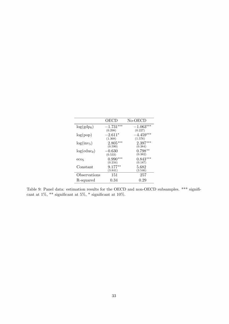
OECD No-OECD

log(gdp0) −1.731(0.298)

∗∗∗ −1.063(0.227)

∗∗∗

log(pop) −2.611(1.368)

∗ −4.459(1.576)

∗∗∗

log(inv5) 2.805(0.590)

∗∗∗ 2.397(0.384)

∗∗∗

log(educ0) −0.630(0.533)

0.798(0.382)

∗∗

eco5 0.990(0.234)

∗∗∗ 0.843(0.187)

∗∗∗

Constant 9.177(3.841)

∗∗ 5.682(3.546)

Observations 151 257R-squared 0.34 0.29

Table 9: Panel data: estimation results for the OECD and non-OECD subsamples. *** signifi-cant at 1%, ** significant at 5%, * significant at 10%.

33

Variable (i) (ii) (iii)Group 1

(32%)Group 2

(68%)Group 1

(32%)Group 2

(68%)Group 1

(32%)Group 2

(68%)

Intercept 0.232(2.369)

10.220(3.227)

∗∗∗ 0.193(2.363)

10.224(3.228)

∗∗∗ 0.206(2.724)

9.040(3.479)

∗∗∗

log(gdp0) −0.507(0.249)

∗∗ −1.121(0.207)

∗∗∗ −0.509(0.250)

∗∗ −1.119(0.207)

∗∗∗ −0.421(0.273)

−1.024(0.221)

∗∗∗

log(pop5) 2.675(0.848)

∗∗∗ −7.233(1.405)

∗∗∗ 2.6813(0.845)

∗∗∗ −7.237(1.411)

∗∗∗ 2.458(0.956)

∗∗ −5.649(1.485)

∗∗∗

log(inv5) 1.383(0.454)

∗∗∗ 2.649(0.359)

∗∗∗ 1.393(0.448)

∗∗∗ 2.645(0.363)

∗∗∗ 1.583(0.689)

∗∗ 2.534(0.376)

∗∗∗

log(educ0) −1.839(0.426)

∗∗∗ 0.715(0.348)

∗∗ −1.832(0.419)

∗∗∗ 0.717(0.349)

∗∗ −2.061(0.540)

∗∗∗ 0.514(0.422)

eco5 0.343(0.144)

∗∗ 0.929(0.169)

∗∗∗ 0.93(0.169)

∗∗∗ 0.296(0.111)

∗∗∗

reg5 0.343(0.142)

∗∗ 0.674(0.192)

∗∗∗

time dummies .. .. ... .. .. ..

Concomitant variablesIntercept - −6.692

(1.896)

∗∗∗ - 7.527(2.123)

∗∗∗ - 14.916(4.763)

∗∗∗

xcont30 - −0.639(0.322)

∗∗ - - −1.719(0.652)

∗∗∗

freedom30 - - −0.823(0.37)

∗∗ -

log(educ1970) - −0.199(0.793)

- 0.004(0.802)

- −0.839(1.647)

lat - −2.249(4.349)

- −3.287(4.379)

- −3.307(6.255)

OECD - −2.335(1.330)

- −1.892(1.336)

- −2.36(1.912)

landlocked - −2.689(1.249)

∗∗ - −2.678(1.245)

∗∗ - −3.848(1.769)

∗∗

R2 0.54 0.38 0.53 0.38 0.50 0.31BIC 1846.8 1845.4 1627.1CAIC 1876.8 1875.4 1651.1

Table 10: Panel data: estimation results of the selected models for the robustness *** significantat 1%, ** significant at 5%, * significant at 10%. Due to some missing data for the measureof regulation(reg5) the number of observations falls to 362 observations in column (iii), but thenumber of countries does not change

34

Variable Period 1970-1985 Period 1985-2000Mixture Mixture

group 1(28%)

group 2(72%)

group 1(28%)

group 2(72%)

Intercept 3.913(4.217)

10.816(5.709)

∗ 0.355(3.384)

9.377(3.801)

∗∗

log(gdp0) −0.723(0.424)

∗ −1.306(0.342)

∗∗∗ 0.03(0.419)

−1.095(0.249)

∗∗∗

log(pop5) 1.889(1.080)

∗ −6.385(2.449)

∗∗∗ 4.281(1.293)

∗∗∗ −6.462(1.597)

∗∗∗

log(inv5) 1.599(0.689)

∗∗ 2.574(0.594)

∗∗∗ −0.304(0.983)

2.011(0.414)

∗∗∗

log(educ0) −2.235(0.630)

∗∗∗ 0.951(0.540)

∗ −3.588(0.772)

∗∗∗ 0.773(0.454)

∗

eco5 0.232(0.157)

0.704(0.302)

∗∗ 0.465(0.222)

∗∗ 1.093(0.206)

∗∗∗

time dummies .. .... ... ...

Concomitant variablesIntercept - 15.395

(4.965)

∗∗∗ - 12.263(3.724)

∗∗∗

dem15 - −0.805(0.334)

∗∗ - −1.032(0.418)

∗∗

log(educ70) - −4.827(1.588)

∗∗∗ -

log(educ85) - - −1.467(1.074)

landlocked - −6.442(2.752)

∗∗ - −2.854(1.656)

∗

R2 0.67 0.27 0.58 0.41BIC 912.6 984.5CAIC 934.6 1006.5

Table 11: Panel data: estimation results of the selected mixture model by subsamples. There are71 countries with 190 observations for the first subsample, and 74 countries with 216 observationsfor the second subsample. *** significant at 1%, ** significant at 5%, * significant at 10%.

35

Variable 2SLS 2SLSGroup 1

(28%)Group 2

(72%)

intercept −0.036(2.448)

11.34(3.328)

∗∗∗

log(gdp0) −0.490(0.217)

∗∗ −1.190(0.218)

∗∗∗

log(pop5) 2.330(0.944)

∗∗ −7.407(1.402)

∗∗∗

log(inv5) 1.179(0.493)

∗∗ 2.784(0.365)

∗∗∗

log(educ0) −1.485(0.470)

∗∗∗ 0.812(0.395)

∗∗

eco5 0.416(0.168)

∗∗ 0.805(0.193)

∗∗∗

time dummies ... ...

nobs 112 219ncountries 24 50Hausman test 0.03 0.55Weak instr. 328.10 370.27

Table 12: IV estimations by groups, from the classification obtained in Table 7 (standard errorsin parenthesis). First lags of log(educ0), dem5 and eco5 are used as instruments. For Hausmantest, the p-values are reported. For weak instruments test, the value of the first-stage-F statisticis reported. *** significant at 1%, ** significant at 5%, * significant at 10%.

36