Polarized supersonic plasma flow simulation for charged...

PHYSICAL REVIEW E VOLUME 52, NUMBER 5 NOVEMBER 1995

Polarized supersonic plasma flow simulation for charged bodies such as dust particles and spacecraft

F. Melands01 and J. Goree2•* 1The Auroral Observatory, University ofTromsD, N-9037 TromsD, Norway

2Department of Physics and Astronomy, The University of Iowa, Iowa City, Iowa 52242 (Received 23 June 1995)

When an object such as a dust particle or spacecraft is immersed in a plasma flowing at a supersonic speed, an asymmetric screening potential forms around that object. The asymmetry is especially pronounced on the downstream side, with an ion rarefaction in the wake followed by an ion focus region. This polarized screening potential helps explain recent laboratory results with dusty plasmas, where collective interparticle effects were shown to be asymmetric. Using an electrostatic fluid simulation with cold ions and Boltzmann electrons, we have simulated the flow around spherical and cylindrical bodies, with and without a negative potential bias. Here, the flow speed v0 is assumed to be supersonic (faster than ion acoustic) and mesothermal ( vTi << v0 << Vre ). A numerical method is used, with a diffuse object that simulates the ion loss and space charge on an object's surface. This works with one or many objects, of any shape. We present solutions for systems of one and two particles in a simulation box, with periodic boundary conditions that help reveal collective effects.

PACS number(s): 52.40.Hf, 52.65.-y, 52.35.Tc

I. INTRODUCTION

Supersonic flow of a plasma onto a solid object is of interest for dusty plasmas and for spacecraft in low Earth orbit. A dusty plasma is a low-temperature ionized gas containing small solid particles, which become charged by absorbing electrons and ions from the plasma [1]. A spacecraft becomes charged for the same reason [2,3]. Since the ratio of the object size to Debye length is roughly the same for a dust particle in a laboratory plasma as for a spacecraft in the ionosphere, the physics presented here applies equally to spacecraft and laboratory dusty plasmas. The term "object" will be used here to refer equally to a dust grain or a spacecraft.

Numerous theoretical and experimental studies of the problem of supersonic flow into an object have been reported for both space and laboratory plasmas. Charging of a spacecraft in the ionosphere was the subject of early theoretical [4] and numerical [5] studies. They predicted a so-called plasma wake (rarefaction in the ion density) immediately downstream of the spacecraft followed by an ion focusing region (high ion density) farther downstream. The wake itself is due to the finite size of the object, while the ion focusing is an electrical effect that will appear regardless of the object size. The wake region was clearly indicated by measurements around the space shuttle (6]. Both the wake and focus regions have been detected in laboratory experiments [7 -9]. Often particulates are found in a sheath or double layer, where there is an electric field that accelerates the ions to supersonic ve-

*Electronic address: [email protected]

1063-651X/95/52(5l/5312( 15)/$06.00 52

locities, as required by the Bohm sheath criterion. A recent particle-in-cell simulation by Choi and Kushner [10] showed that wake and focusing effects may be important for the charging of dust particles in gas discharge plasmas. They looked at the charging of two particles, aligned so that one particle shadows the other, and found a significant difference in the surface potential of the two particles.

Theoretical techniques also can be used to find approximate solutions for the electric field and plasma density distribution around a charged object, moving at a velocity v0 relative to the plasma. Several methods are described by Al'pert et a/. [4]. Some of these invoke quasineutrality, which is an unsuitable approximation. This is improved by solving the Poisson equation, which has been done in a Vlasov approach by several authors, as reviewed by Coggiola and Soubeyran (3]. A linear test particle approach (11,12] is also possible (see Sec. V) although it does not include any loss of plasma particles, which is required for plasma wake effects. Test particle calculations by Chenevier, Dolique, and Peres [13] have shown that the Mach number M =v0 !c;, where c; is the ion acoustic velocity, is an important parameter for the shielding. Note that this Mach number is not defined using the ion thermal velocity, a distinction that is especially important for gas discharges where T; << Te is typical for the ion and electron temperatures. The symmetry of the screening depends on the regime of the flow speed, as summarized in Fig. 1. The screening is symmetric, i.e., the same on the upstream and downstream sides, for flow velocities well below the ion thermal speed, v0 <<uTi. Asymmetric shielding occurs in a regime extending from slightly below the ion thermal speed to slightly above the acoustic speed. In highly supersonic flows, v0 >>c;, ion orbits are undeflected and thus do not screen the charged object, resulting in symmetric screening, due to the electrons alone.

5312 @ 1995 The American Physical Society

52 POLARIZED SUPERSONIC PLASMA FLOW SIMULATION FOR ... 5313

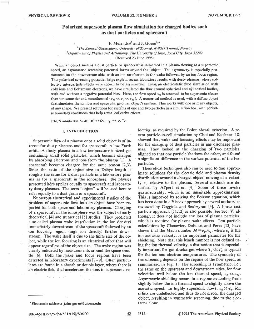
: ' ......-:..----------.:-symmetric , asymmetric : symmetric screening screening screening (electrons (electrons (electrons

& ions) & ions) only)

mesothermal regime (cold ions & Boltzmann electrons)

FIG. 1. The regimes of flow speed and screening for a charged object in a plasma flowing at velocity v0 • For this sketch, Ti < Te. Our simulations are carried out for velocities that are supersonic and in the mesothermal regime.

The mesothermal regime, which we have simulated, is specified by the velocity range vTi << v0 << Vre. It is typical of both a particle in a gas discharge and a spacecraft in low Earth orbit. In a laboratory plasma, micrometersized dust particles are typically found near the edge of an electrode sheath, where the ion drift velocity has M = 1, or within the sheath, where M > 1. In low Earth orbit, oxygen ions flow toward a spacecraft with an energy of 5 eV, which is supersonic.

In this paper we report numerical solutions of a selfconsistent fluid model describing the plasma flow into a charged object. The simulation was carried out in three dimensions (30) for a spherical object and in 20 for a cylinder aligned perpendicular to the flow. The plasma flow velocity v0 is assumed to be supersonic (M > 1).

We use a two-fluid model with cold ions and Boltzmann electrons in an unmagnetized plasma, and a fixed potential on the surface of the object in the plasma. Using Boltzmann electrons is a good approach for mesothermal flows where vTi <<v0 <<vre· Our fluid approach should offer a good description of the overall structure of the flow, but it will not reveal kinetic effects such as electron heating, thermal wake filling, or velocity-space instabilities in the wake and ion focus region. The unmagnetized plasma assumed here is suitable when the ion Oebye length and object diameter are very small compared to the gyroradius. For dust particles in a gas discharge this requirement is easily satisfied. It is somewhat less applicable to spacecraft in low Earth orbit, where the cyclotron motion of ions alters the wake, as shown in experiments aboard the space shuttle [6].

The polarity of the potential on the object is a crucial factor in determining the structure of the flow. We consider here only negative potentials. Of course this attracts ions, which is readily apparent in our results. Negative potentials are typical of laboratory dusty plasmas and of some cases with spacecraft and dust in space. Positive potentials, however, develop sometimes on spacecraft, due to photoelectric or secondary electron emission.

The geometry assumed in our numerical method is nonperiodic along the streaming direction and periodic in the transverse directions. Periodic boundary conditions introduce collective effects since ghost objects are regularly spaced outside the computational domain. Collective effects can be enhanced by reducing the spacing Ly (and Lz for the 30 case) in the periodic directions and introducing several objects in the nonperiodic x direction. Collective effects are discussed further in Sec. III B.

We report a method of using a diffuse body to simulate a solid object in the plasma. The key physics that must be retained are the surface charge and the surface collection of plasma ions. In a diffuse body, the charge and ion loss are distributed throughout the object's volume. The diffuse body is described by a distribution function S ( x) in the spatial coordinate x, as discussed in Appendix A.

We were motivated by two types of recent laboratory experiments with dusty plasmas. High-power sputtering plasmas produced unusual arrangements of particles that had coagulated [14], and low-power discharges levitated microspheres in a way that they were spaced in a crystallinelike lattice [15-17]. There were two surprising observations that might be explained by collective effects involving dipole attraction. One is that the conglomerate that forms from coagulation is string shaped rather than fractal-like (as expected for isotropic coagulation) when they collide and stick [14]. Another is the vertical alignment of microspheres in the plasma crystals [15-17]. While it is not surprising that the spheres arrange themselves in hexagons in horizontal planes (perpendicular to the flow), it was unexpected that they tend to align directly above one another, rather than staggered as in bee and fcc crystalline structures. These experimental observations suggest that the interparticle potential is not strictly an isotropic repulsive monopole repulsion, but might include an anisotropic dipole attraction.

Our simulation reveals that the wave effect causes the flowing plasma in the vicinity of a charged object to have a significant polarization and dipole moment. It also causes the ion flux collected by the object to differ on the up and downstream sides, leading to a polarization of the object itself, if it is nonconducting. These polarizations of the plasma and the object will lead to interparticle dipole forces that are attractive parallel to the flow, thereby partially overcoming the repulsive monopole forces between two negative charges. The force between a particle and its own sheath is also influenced by a dipole moment in the sheath [18,19].

The flowing plasma considered here is not the only way the sheath can acquire a dipole moment. A plasma nonuniformity, such as a density gradient and an external electric field, also polarizes the sheath. A density gradient corresponds to a gradient in the Oebye length, leading to a slight positive potential region on the highdensity side of the sheath. This effect was studied by Hamaguchi and Farouki [18,19]. They were chiefly concerned with finding the force on a single isolated particle in a laboratory plasma. Our results are also revealing for the behavior of a single particle, but it is collective effects between multiple charged particles that we are most concerned with explaining.

5314 F. MELANDS0 AND J. GOREE 52

II. FLUID EQUATIONS

The plasma is modeled by a cold ion fluid and Boltzmann electrons, which respond self-consistently to the Poisson equation. With this treatment, the ions have a density n; and a flow velocity V; while the electrons are characterized merely by a prescribed uniform temperature Te and a density

(1)

Here n0 is the ion density at a point well away from any object in the plasma.

In computing the flow of the ions around the object, we model the ion absorption with loss terms in the continuity and momentum equations. In the Poisson equation, a fixed charge is specified, and it is assumed to be uniformly distributed on the surface, neglecting the tendency of the upstream side to collect more ions and charge more positively than the downstream side [3]. Based on our results, we will discuss later in qualitative terms how this nonuniform charging will take place.

The continuity and momentum equations for the ion fluid can be written with the ion loss on the right-hand side:

(2)

Here the ion mass, electronic charge, and flow velocity are denoted m;, Z;, and V;, while rand r 0 represent the position vector and the object's surface, respectively.

The ion loss in the continuity equation is the ion flux, y i• multiplied by a Dirac delta function 8, which describes the object's surface. For a perfectly absorbing surface, the ion flux at the surface can be written as [4]

= ~-n;v;·n for v;·n<O,

Y; o for v;·n>O. (4)

Here n is a unit normal vector to the surface (pointing outward).

In the momentum equation [Eq. (3)] we have assumed cold collisionless ions by neglecting the pressure and collision terms. Since the object in the plasma is massive, ions are assumed to lose all their momentum when they strike. The momentum equation can be rewritten by combining it with Eq. (2) to yield

eZ; a 1v;+v;·Vv;=---V¢J,

m;

where the ion loss term has conveniently canceled out.

(5)

The plasma flow is assumed to be irrotational. This is valid provided it is irrotational as it enters the simulation region, since the circulation is a conserved quantity for our conservative force [right-hand side (RHS) of Eq. (5)] [20]. Thus the convective term v;·Vv; can be written as V( vl /2) and the momentum equation [Eq. (5)] becomes

(6)

The Poisson equation is

V2ifJ=- ~[n; -ne +zd8(r-r0 )/p] , Eo

(7)

where zd is the total number of elementary charges ·uniformly distributed on the surface, and p=2rrr0 or 4rrr5 for a cylindrical or spherical surface, respectively.

The full set of fluid equations we will solve are Eqs. (1 ), (2), (4), (6), and (7). These equations can be cast in dimensionless form by normalizing all the variables: T=wp;t, X=x/A.ne• V=v;/C;. N=n;ln 0 , Ne=neln 0 , .::l=8A.0 e, r=y;fwp;Aoen0 , Zd =zd /pn 0 A.0 e, and = -e¢1/KTe. The time has been normalized by the ion plasma frequency wp; =(e 2Zln 0 /E0m; )112

, where the density n; at a large distance from the object on the upstream side is specified as n0 . Distance is normalized by the electron Debye length "-ne=(EoKTe/e 2n0 )

112, which is consistent with

normalizing velocities by the ion acoustic velocity c;=(ZlkB Telm; )112

.

The continuity, momentum, and Poisson equations in dimensionless form become

aTN+Vx·(NV)=-ra(X),

aTV+Vx(V2/2)=Vx<l>,

Vi=N -exp( -)+Zd.::l(X).

(8)

(9)

(10)

For the loss term, the flux r can be written in terms of the Heavyside step function Has

r=-NV·nH(-V·n). (11)

For given boundary and initial conditions, this selfconsistent set of equations can in principle be solved, We do this numerically in a rectangular simulation box, using the method described in Appendix B. The flow is in the positive X direction, and the component of the velocity V in that direction is denoted U.

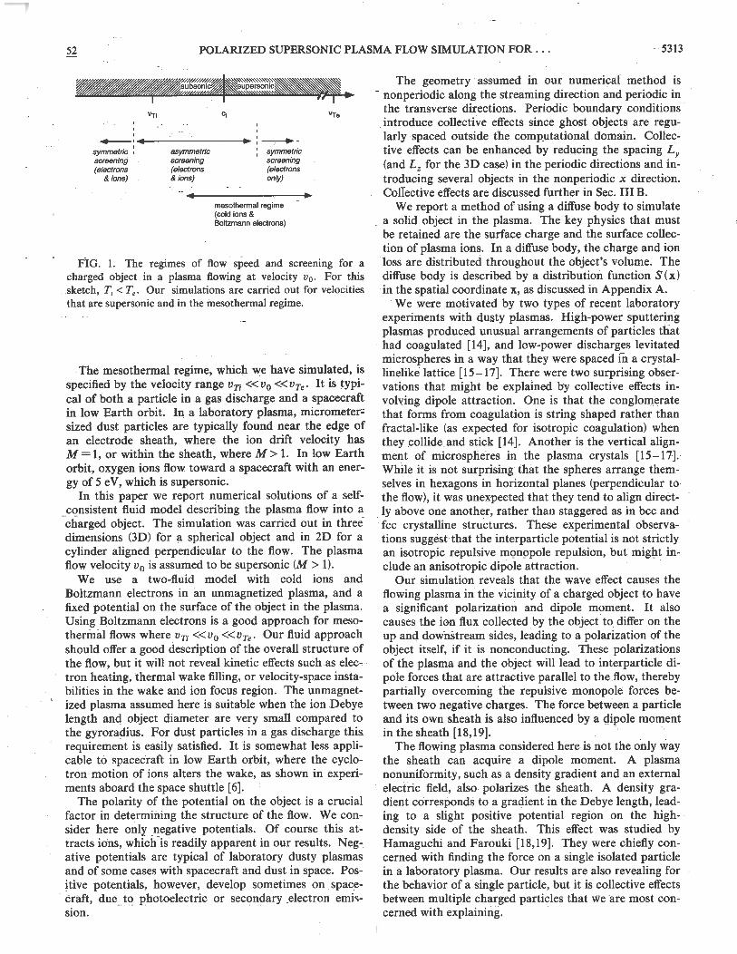
The boundary conditions, which are summarized in Fig. 2, include specifications of the density, velocity, and electrical potential on the sides of the simulation box. The boundary conditions are periodic in the transverse direction and nonperiodic parallel to the flow (X direction). For supersonic flows (M > 1) given by Eqs. (8)-(11), boundary conditions for N and U must be specified only on the upstream side (X= 0) of the box, while must be specified only on the downstream side (X=Lx ). However, in our numerical solutions we also were required to specify gradients of N and U on the· downstream sides, because we added small diffusion and viscosity terms to Eqs. (8) and (9), respectively (see Appendix B for more details). This changed the character of Eqs. (8) and (9) from hyperbolic to parabolic, requiring that Nand U also be specified on the outflow boundary.

Neumann boundary conditions were used on the downstream edge of the simulation box

(12)

52 POLARIZED SUPERSONIC PLASMA FLOW SIMULATION FOR .. . 5315

y

X

inflow boundary conditions:

ion flow 'I = M Cs ion density ni = no

potential q, = 0

~ I

downstream region (wake and ion focus)

: L center line

L simulation box

FIG. 2. Computation domain and boundary conditions used in the 2D and 3D simulations. The flow enters a rectangular simulation box from the top with a velocity v0 =Me; in the X direction. In 3D, the box is the same in the Y and Z directions. The object is a cylinder (2D simulation) or a sphere (3D), and it is diffuse; i.e., it does not have a distinct surface. Our solutions are assumed to be nonperiodic in this direction and periodic in the transverse directions. Dirichlet and Neumann boundary conditions are used for the inflow and outflow sides, respectively in the X direction. Periodic boundary conditions used in the other directions lead to ghost particles outside the computation domain, which for a dusty plasma simulates collective effects. In the simulation results presented below, only the left half of the simulation box is shown, since the problem is symmetric about the center line. ..... t---Ly

outflow boundary conditions:

au ;aX(X=Lx, Y,Z)=O,

a;aX(X=Lx, Y,Z )=0

ilv;/ilx=O

iln; /ilx= 0

ilq,/ilx= 0

(13)

(14)

and Dirichlet boundary conditions on the upstream edge

N(X=O,Y,Z)=1,

U(X=O, Y,Z)=M,

(X=O, Y,Z)=O.

(15)

(16)

(17)

Intuitively, one would expect the Neumann boundary to be physically correct far downstream from a charged object, where the disturbance due to geometrical effects and shielding by the plasma is small. However, our numerical tests show that even if the downstream boundary is close to the charged object, using Neumann boundary conditions results in only a very small disturbance in the plasma flow as it propagates out of the simulation box.

In addition to the boundary conditions, we also must specify initial conditions. The exact choice is not important, as we shall only seek the steady-state solution. At T=O we used the initial conditions

N = 1 , U=M , <1>=<1>0 , (18)

where the flow is initially in the X direction and <1>0 is the

initial potential found by solving the Poisson equation [Eq. (10)) with a uniform ion density N = 1.

III. THE OBJECT IN THE PLASMA

A. Numerical treatment of the object

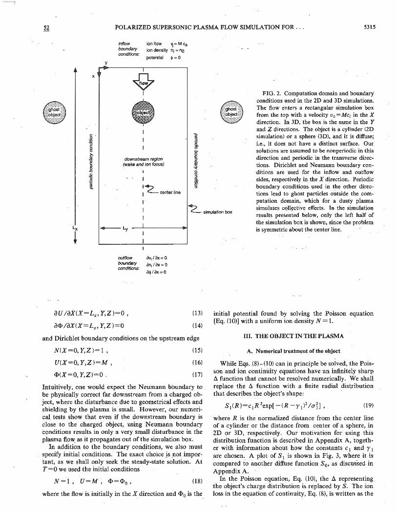
While Eqs. (8)-(10) can in principle be solved, the Poisson and ion continuity equations have an infinitely sharp 1::. function that cannot be resolved numerically. We shall replace the 1::. function with a finite radial distribution that describes the object's shape:

(19)

where R is the normalized distance from the center line of a cylinder or the distance from center of a sphere, in 2D or 3D, respectively. Our motivation for using this distribution function is described in Appendix A, together with information aboUt how the constants C 1 and y 1

are chosen. A plot of S 1 is shown in Fig. 3, where it is compared to another diffuse function S0 , as discussed in Appendix A.

In the Poisson equation, Eq. (10), the 1::. representing the object's charge distribution is replaced by S. The ion loss in the equation of continuity, Eq. (8), is written as the

~

J!J ·~ 0.8

-e .. --; 0.6 0 .B 1:

~ 1: 0.4 0 ·.:; :::l

.LJ

·~ 0.2 :u

0 0 0.5 1.5 2 2.5

radial distance R = r I A.oE

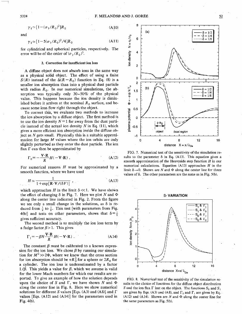
FIG. 3. Distribution function S of a diffuse object. This function replaces the delta function representing the object's surface in the Poisson and ion continuity equations. The dimensionless distance R = r /A.oe is measured from the center of a spherical or cylindrical object. The two functions shown are given by Eqs. (A3) and (A8). In these plots the parameters R 0 =l, a 0 =a 1=0.5y0=l, and y 1=t were used, for a diffuse cylinder.

product r 1S 1 (R ), where the flux into the diffuse object is

V·R r 1 =-/3N--H(- v · Rl R . (20)

The factor /3 > 1 corrects for insufficient ion loss, as explained in Appendix A.

B. Collective effects for dusty plasmas

In a dusty plasma there can be many charged dust particles per unit volume. This is mimicked in our simulation by using periodic boundary conditions, which provide ghost particles at a regular spacing. For this reason, we summarize here the use of a parameter P, which is a common measure of the dust particle density [21]. This parameter is defined as

(21)

and it depends on eu !KTe, where u is the particle potential with respect to the surrounding plasma potential. For eu I KTe of the order of unity (which is typical for solid objects in a thermalized electron/ion plasma), P can be used to determine whether a solid object can be assumed to be isolated (P << 1) or if collective effects are dominant (P?. 1).

To use Eq. (21) for charged objects, we find the charge on the object as Zd = Cu I e and model C as the capacitance of two concentric conductors. For spheres, the inner conductor is placed at r 0 (the radius of the object's surface) and the outer at r0 + Ane (the Debye sheath edge) so that C=47TE0r0 ( 1 +r0 /A.0 e). Using the normalization R o = r 0 I Ane• this yields

(22)

where Lx, Ly, and Lz are the mean separations between the particles in the x, y, and z directions. Similarly, for cylindrical objects the capacity per unit length of two concentric cylinders is C = 27TE0 /ln( 1 + Anelr0 ) giving

(23)

IV. RESULTS

Our simulation yields spatial profiles of the steady-state ion density and electric potential. These are our main results, shown in the color plots Figs. 4 and 5. The ion density is shown in the upper half of these figures, and the plasma potential in the lower half. The plasma flows into the simulation box from the top, parallel to the X axis.

We use a spectral method to solve the fluid equations, Eqs. (8)-(10). This is done with boundary conditions Eqs. (12)-(17) and initial conditions Eq. (18). In our solutions the steady state was reached after a time of 40/wp; with Mach number M= 1. 5 and 20/wp; for M = 3. 0. Details of the numerical method are presented in Appendix B.

Our simulation of the flow was carried out for a single object (Fig. 4) and for two objects aligned parallel to the flow (Fig. 5). Results for a 3D simulation of a sphere are shown in Figs. 4(d), 4(e), and 5(e), while the panels in Figs. 4(a)-4(c) and Figs. 5(a)-5(d) show 2D calculations with a cylindrical object (axis aligned perpendicular to the flow). The reader should refer to Fig. 2 for the geometry and axis coordinates in Figs. 4 and 5. Half the simulation box is shown in a cross-sectional view, since the problem is symmetric about the vertical axis passing through the objects. In examining these figures, recall that the object is diffuse. The black circle on these figures indicates the nominal radius of the diffuse object, R 0 , but the diffuse object has a charge and ion absorption that is finite both inside and outside this radius. The diffuse nature of the object means that there is a finite ion density everywhere, even at the center of the object. Also recall that the density n; is normalized by its value on the inflow side, N=n;fn 0 , and the potential ifJ is also normalized, but with a reversed polarity so that a negative bias on the object appears as a positive value of = -eifJ/KTe.

The parameters used in the simulations for the diffuse object were R 0 = 1 (radius equal to the De bye length at the inflow side), and a profile width half that large, a 1 = 0. 5. Except as noted, the size of the simulation box was Lx = 16 and Ly = 8, and for the 3D simulations the Z dimension was Lz = 8.

A. One object in a plasma

For a single object in the plasma, our calculations simulate the problem of a spacecraft or an isolated particulate in a plasma. Or more precisely, they simulate a planar array of such objects, separated fairly widely by 8 Debye lengths, due to the periodic boundary conditions.

To assess the importance of the electric potential on

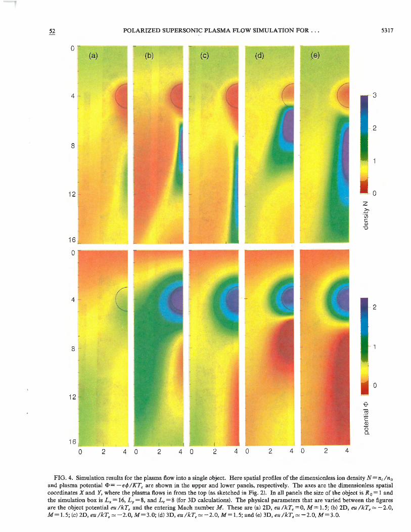
52 POLARIZED SUPERSONIC PLASMA FLOW SIMULATION FOR . .. 5317

(a) (b) (6} (d) (e)

4 3

2

8

12 0

z ~ "Vi c Q)

""0

16

0

4 2

8 -

0

12

16

0 2 4 0 2 0 2 4 0 2 4 0 2 4

FIG. 4. Simulation results for the plasma flow into a single object. Here spatial profiles of the dimensionless ion density N = ni Jn 0

and plasma potential = -e¢J/KT. are shown in the upper and lower panels, respectively. The axes are the dimensionless spatial coordinates X and Y, where the plasma flows in from the top (as sketched in Fig. 2). In all panels the size of the object is R 0 = 1 and the simulation box is Lx = 16, Ly = 8, and Lz = 8 (for 3D calculations). The physical parameters that are varied between the figures are the object potential eu/kT. and the entering Mach number M. These are (a) 2D, eu/kT.=O, M=1.5; (b) 2D, eu/kT.~-2.0, M=1.5; (c) 2D, eu/kT.~ -2.0, M=3.0; (d) 3D, eu/kT.~ -2.0, M=1.5; and (e) 3D, eu/kT.~ -2.0, M=3.0.

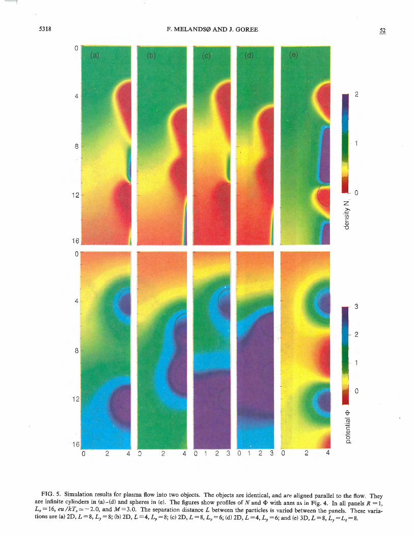
5318

0

4

8

16

0

4

8

F. MELANDS0 AND J. GOREE 52

2

0

3

2

- 0

FIG. 5. Simulation results for plasma flow into two objects. The objects are identical, and are aligned parallel to the flow. They are infinite cylinders in (a)-(d) and spheres in (e). The figures show profiles of Nand ct> with axes as in Fig. 4. In all panels R = 1, Lx=l6, eu/kT.~-2.0, and M=3.0. The separation distance L between the particles is varied between the panels. These variations are (a) 2D, L = 8, Ly = 8; (b) 2D, L =4, Ly = 8; (c) 2D, L = 8, Ly =6; (d) 2D, L =4, Ly = 6; and (e) 3D, L = 8, Ly = Lz = 8.

the object, we first ran the simulation with a zero potential, relative to the plasma at the inflow side. The results in Fig. 4(a) show that even when the object is unbiased, there is a wake (ion rarefaction) and an ion focus region (enhanced ion density) that form behind it. The ion loss on the object accounts for this disturbance of the plasma. The wake and ion focus appear as red and green regions, respectively, in the density profile of Fig. 4(a). The reason for the ion focus region is that the wake has an enhanced potential that attracts ions, causing them to stream inward toward the central axis at the same time as they stream downward. These results are forM= 1.5.

When the object has a finite negative potential, it attracts ions. This leads to a shorter wake and a stronger ion focus region, compared to the unbiased object at the same Mach number. The enhanced ion focus effect is seen in the density profile of Fig. 4(b) as a purple region along the axis downstream of the object. We also see a (green) cone of ion density propagating downward and outward from the focus. This is probably an ion acoustic wave generated by compression .in this region. The number of elementary charges on the object Zd was chosen in this figure, and also in Figs. 4(c)-4(e), to yield a plasma potential - 2 through the diffuse object. This simulates a physical object with negative surface potential eu I KTe = -2. 0. This is typical for a dust particle in a laboratory plasma.

A higher Mach number leads to a larger downstream extension of the wake and focus regions. This is shown in Fig. 4(c), where the Mach number was M=3.0, twice that of Fig. 4(b). The wavelike cone is also compressed to a smaller angle.

All the results discussed above are from a 2D simulation for an infinite cylinder. Now we turn to the 3D simulation for a spherical body. Results are shown in Figs. 4(d) and 4(e) for M = 1. 5 and 3.0, respectively.

The ion focus region is greatly enhanced for a sphere, as compared to a cylinder. The wake, on the other hand, is smaller for a sphere. This is probably a geometrical effect, since the sphere attracts ions from all around it, including both the Y and Z directions compared to only the Y direction for a cylinder. At the higher Mach number, the focus region is extended farther downstream and the wavelike cone has a smaller angle, similar to the results for a cylinder.

One of the most significant results to note is the polarization of the plasma around the diffuse object. It can be seen most easily in the plasma potential profiles (lower panels in the figures). The normalized potential = -efjJ/KTe is much more positive within and near the diffuse object, and less positive or even negative in the focus region.

The polarization of the plasma surrounding the object means that the object together with the nearby plasma is a dipole. Within the object and in the wake region the space charge is negative, due to the object's negative bias and the low ion density in the wake. The focus region, on the other hand, contains a positive space charge due to a high ion density.

If the uniform potential on the object assumed in the simulation were replaced by a dielectric surface, the ob-

ject itself would gain a dipole moment that would add to that of the plasma. Polarization of the object would be significant mainly if the object size is not much smaller than the Debye length.

B. Two objects in a plasma

By placing two objects in the plasma so that they are aligned parallel to the flow, we can better simulate collective effects between charged particulates. These calculations are relevant to dusty plasma experiments, as discussed in Sec. V.

Two identical particles were placed in the simulation box, with the downstream one positioned in the wake or focus region of the upstream particle. In Figs. 5(a)-5(d) the particles are cylindrical, and in Fig. 5(e) they are spheres. All the results shown are for M = 3. 0. The Y spacing (transverse to the flow) was reduced to Ly = 6 in Figs. 4(c) and 4(d) to test the effect of a higher dust particle number density. Otherwise the same parameters were used as in Fig. 3.

When two particles are spaced closely in the direction of the flow, the ion focus region between them disappears. This is seen in comparing Figs. 5(a) and 5(b), where the spacing is L = 8 and 4 Debye lengths, respectively.

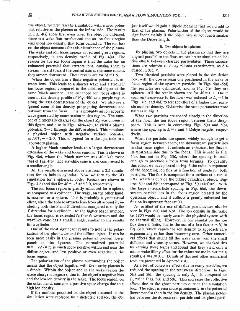
When the particles are spaced widely enough to get a focus region between them, the downstream particle lies in that focus region. It collects an enhanced ion flux on its upstream side due to the focus. This is seen in Fig. 5(a), but not in Fig. 5(b), where the spacing is small enough to preclude a focus from forming. To quantify this effect, we have plotted in Fig. 6 the radial component of the incoming ion flux as a function of angle for both particles. The flux is computed for a surface at a radius 2R 0 , which is outside the diffuse cylindrical object. Figures 6(a) and 6(b) correspond to Figs. 5(a) and 5(b). With the large interparticle spacing in Fig. 6(a), the downstream particle lies in the focus region created by the upstream object, and it collects a greatly enhanced ion flux on its upstream face (at o·).

An artifact of the use of diffuse particles can also be seen in Figs. 6(a) and 6(b). The ion density in the wake (at 180•) would be nearly zero in the physical system with no thermal filling. However, in our simulation the ion flux there is finite, due to the use of a loss factor a: N, in Eq. (20), which causes the ion density to approach zero exponentially rather than becoming zero. Other numerical effects that might fill the wake arise from the small diffusion and viscosity terms. However, we checked this by varying these terms and found that they yield only a minor wake-filling effect for the values we use in our main results, E1 =£2 =0.1. Details of this and other numerical tests are presented in Appendix A.

As a test of collective effects due to many particles, we reduced the spacing in the transverse direction. In Figs. 5(c) and 5(d), the spacing is only Ly =6, compared to Ly = 8 in Figs. 5(a) and 5(b). This increases the collective effects due to the ghost particles outside the simulation box. The effect is seen more prominently in the potential (lower panels) than in the ion density. The plasma potential between the downstream particle and its ghost parti-

cle is enhanced. Plasma with a large (more negative plasma potential </J) fills the region between downstream particles.

There are two effects that cause the plasma potential to be modified when particulates are closely packed. One phenomenon is the depletion of plasma electrons due to the negative charge on the particulate. This effect is parametrized by the value P [21], given in Eqs. (22) and (23). Second is the absorption of ions due to the finite size of the particulate. Both of these collective effects lead to a plasma potential </J that is negative, compared to the infinite plasma. This is also in good agreement with the lower panels in Figs. 5(a)-5(d), where decreasing the particle spacing causes the normalized potential = -e</J/KTe to increase to a higher positive value throughout the simulation box, relative to the infinite plasma on the inflow side of our simulation box. In phys-

(a)

(b)

-- upstream object ···-···· downstream object

0

180

0

90

180

FIG. 6. The ion flux collected by two cylindrical objects. The data in (a) and (b) correspond to Figs. 5(a) and 5(b), respectively. The flux was calculated at a radius R 0 , which is outside the diffuse body. Far more ions are collected on the inflow side, o•, than on the outflow side, 180·. In (a), the downstream object lies in the beamlike ion focus region of the upstream object, and it collects an enhanced ion flux concentrated at o·.

ical systems the second effect (absorption) is usually smaller than the first one, when r 0 /Aoe << 1, which is typical in space and laboratory dusty plasmas. This condition is not met in our numerical solutions, where our choice of r 0 = Aoe probably leads to significant collective effects.

Spherical particles were simulated in 3D in Fig. 5(e). Other parameters were the same as in Fig. 5(a), which is for cylindrical objects. The potential distribution around the downstream particle is nearly the same as around the upstream one. This is probably because the parameter P is smaller for the spherical simulation than for the cylindrical. For the sphere in Fig. 5(e), P =0. 049, which is only one-third of the value P =0. 14 for the cylinders in Fig. 5(a). These values were computed by doubling the results from Eq. (22) and Eq. (23), since our simulation box contains 2 particles. Despite our use of the same simulation parameters, P varies between these two cases because of the different electrical capacitance of a sphere and a cylinder.

An analytic theory for the dependence of the plasma potential on the parameter P was presented by Havnes, Aslaksen, and Melands0 [21]. It has been adapted by Goree [22] to use a fixed ion density to better simulate discharge conditions. This theory predicts that the plasma potential, averaged over all the volume in a dusty plasma, varies from 0 to about 3 times the electron temperature, as P increases from zero to large values. This model is not strictly comparable to our simulation, because the model neglects ion absorption, and depends slightly on two parameters that do not appear in our model, the ion mass and the ratio of the ion and electron temperatures. Nevertheless, it is possible to make an approximate comparison of our results to the Havnes model. We find that the plasma potential is highly nonuniform in our simulation, and averaging over the simulation volume the potential is modified somewhat more strongly than predicted by the Havnes model. This difference is probably due to ion absorption, which is quite significant for the large (r 0 /A0 e) particles in our simulation. This conclusion is consistent with a comparison of Figs. 4(a) and 4(b), where the plasma potential is modified approximately twice as much when the particle has a negative bias compared to when it is unbiased.

V. DISCUSSION

A. Wake effects

The wake is a. region of low ion density close to the object on the downstream side. It is due to absorption of ions. The extent of the wake should increase with the size of the body. It also depends strongly on the Mach number M and the object charge Zd, as shown in Fig. 4. When the size of an object is comparable to Aoe• as in our numerical calculation, this wake alters the total space charge and creates an asymmetric field around the object. This effect is clearly seen from Fig. 4(a) where the object is uncharged.

For most dusty plasmas in space and laboratory, r0 <<Aoe• and the wake probably will have little effect on

the total space charge. This is because the extent of the wake in the transverse Y direction scales as the particle cross section, which is a: r0 for cylindrical and a: r5 for spherical particles. The volume occupied by the wake would therefore become much less than the plasma volume that determines the Debye screening (sphere with a radius -A.0 e>>r0 around the charged object).

B. Limitations of the Debye-Hiickel and Bernstein-Rabinowitz approximations

Our results verify that the potential is strongly anisotropic in mesothermal flows. This is shown in our numerical solutions and the test-particle approach described below. In view of this, we conclude that central potentials such as the Debye-Hiickel approximation, which includes only electron screening, are accurate for supersonic flows only for high Mach numbers (M >> 1) and small objects r 0 <<Ane so that the wake region does not contribute significantly to the space charge. In subsonic flows, which we have not simulated, the Debye-Hiickel expression is probably valid also in the velocity regime u0 <<ur;, provided that A.ne is replaced by a Debye length that includes both electrons and ions. For dust particulates in gas discharges this low velocity condition will seldom be fulfilled, due to a very low uTi.

Models such as Debye-Hiickel that assume a central potential may have some utility if they are applied only in the plane perpendicular to the flow. In that direction the ion density remains fairly constant. It is along the direction of flow where the potential is most strongly noncentral, with ion focus and wake regions on the downstream side. In that direction Debye-Hiickel is unsuitable for mesothermal flows.

Another model that has been suggested in several papers (e.g., Ref. [18]) uses a Bernstein-Rabinowitz equation for n0 which was derived for Langmuir probes [23]. This equation would replace a Boltzmann relation for the ion density, in cases where T; is low compared to Te. This model will, unfortunately, not be useful for mesothermal flows because of two unsuitable assumptions: ( 1) The theory in Ref. [23] assumes a central potential, which is accurate only for small object at a high Mach number M >> 1. For other velocities, the previously discussed anisotropy will exclude the central force assumption. (2) It also assumes a monoenergetic velocity distribution far from the object with cylindrical or spherical symmetry. This model cannot be applied for a mesothermal flow where ions enter from one direction, or have a finite velocity distribution.

For dusty plasmas in gas discharges, the only use for the expression for n; derived in Ref. [23] seems to be dust in the center of a discharge where u0 <<uTi.

Yet another approach to modeling the potential around an object in a flowing plasma is a test particle method. This neglects ion loss, and thus it can be used only for r 0 << Ane· It is a linear theory that assumes small perturbations in the ion orbits. We therefore expect this theory to be imprecise for highly charged dust particles when u0 is in the subsonic or low supersonic regimes.

C. Polarization of the object surface

The charge on an object in a plasma is due to collecting ions and electrons. If the object is a conductor, charge will adjust on the surface so that the surface is an equipotential. On the other hand, if the object is a dielectric (and in most applications it is) the surface potential need not be the same everywhere.

A dielectric object in a flowing plasma will charge differently. Due to the wake, it will collect few ions on its downstream side, and acquire a more negative potential there. This means that the object will acquire a dipole moment p. The electric force experienced by the particle will include not only the monopole force qdE but also a dipole force. Since p is proportional to the particle size, this will be important mainly for large particles.

In a dusty plasma, a dust grain in the shadow of another will be polarized in an even more irregular way. As shown in Fig. 5, a downstream particle rests in the ion focus region of an upstream particle if they are separated by a sufficient distance. This causes the downstream particle to collect an enhanced ion flux on its nose, but less elsewhere, as shown in Fig. 6(a). On the other hand, if the two particles are not greatly separated, the downstream particle will rest in the wake, where N is diminished, and the ion flux will be reduced on the nose of the object, as shown in Fig. 6(b). In either case, the surface polarization will have a more complicated charge distribution than on an isolated particle.

One might ask whether rotation of the object could average out the unequal collection of ions on the front and back surfaces. The time scales determine whether this can happen. The charge on an object can vary on a time scale called the charging time, which varies inversely with plasma density and the size of the object [1,24]. In ionospheric and laboratory plasmas the plasma density is high enough that the object will charge much faster than it could rotate. This means that rotation would not be a factor.

D. Explanation of observations in dusty plasma experiments

By placing two identical objects in the plasma, we simulate collective effects between charged particulates. These calculations are relevant to dusty plasmas. Of particular interest are two types of laboratory experiments that have been reported recently.

In sputtering plasmas coagulated particles form into an unusual stringlike shape. This has been observed by several experimenters (cf. Ref. [14]). The string shape is quite different from the isotropic fractal shape, which is well known for conglomerates grown by isotropic coagulation. This morphology is strong evidence that before two particles can collide and stick, they interact by a potential that is anisotropic. The polarization of the plasma and the particle itself may explain this phenomenon.

In a second type of laboratory experiment, a crystallinelike lattice forms from particles suspended in the plasma [ 15 -17]. In these so-called plasma crystal ex periments micrometer-sized spheres become charged, and they are electrostatically levitated in_ the plasma above a

horizontal electrode, where there is a balance between gravity and the electric forces. The vertical direction is also the direction of ion flow toward the electrode. Through their interparticle interaction, the microspheres separate themselves by a few Debye lengths, and they arrange themselves in a pattern that is hexagonal, as one would expect, in a horizontal plane. Surprisingly, however, in the vertical direction they usually align in columns; so that the 3D structure is one of hexagons aligned directly above one another with no displacement. This is contrary to the staggered planes familiar in hexagonal close-packed solid crystals. One would expect staggered planes for an isotropic repulsive interparticle potential. This too is a strong experimental indication that the interparticle interaction in a plasma is anisotropic.

In both the coagulation and plasma crystal experiments there is an ion flow where the particles are located. They are typically levitated near the sheath edge, where the ion speed is M = 1. As our results have clearly shown, under these conditions the plasma is asymmetric on the upstream and downstream sides of a particle. This should cause a significant anisotropy that qualitatively is in good agreement with the experimental results.

E. Plasma shielding

Our solutions in Figs. 4 and 5 show a significant polarization of the plasma as it flows around charged cylinders and spheres. This polarization is due to both ion absorption and asymmetric screening of the object charge by the ions.

To understand the latter of these effects we invoke here a test particle approach, which is commonly used in the theory of ordinary dust-free plasmas, to study screening, drag forces, and wave-particle interactions. It does not include ion loss and therefore wake effects, which is suitable if r0 <<Aoe· Even though our numerical simulation does not meet this requirement, the test particle approach is useful to gain an understanding of the nature of the ion screening, and to identify when ion screening is important.

In a test particle approach the plasma potential ¢ is found from the dielectric function D (w,k) of the plasma medium, and can be written in terms of an inverse 3D Fourier transform, as

</J(x)=-1_!!.:!__ J exp(ik·x) dk, 81r3 Eo k 1D (w=O,k)

(24)

where w and k are a wave frequency and wave number. This equation is given in a frame in which the object is at rest. This differs slightly from expressions found in most textbooks on plasma physics, which use the plasma rest frame [11,12].

Although the integral in Eq. (24) in general must be evaluated numerically [13], it is not necessary, since much can be learned about the shielding of the particle by examining the dielectric function D. This is

1 1 cl D(w=O,k)=1+-2-2---2- 2

k Aoe Aoe (k·v0 ) (25)

assuming an isolated object in a cold-ion, Boltzmannelectron plasma.

The first two terms in Eq. (25) correspond to the wellknown Debye-Hiickel shielding of the charged object [11], which is due to electrons only, while the last term contains the screening from the ions. We can compare these terms by taking their ratio

1 s=----cos2(0)M2

(26)

written in terms of the Mach number M and the angle e between k and v0• It should be noticed that this expression will not be valid for angles in the vicinity of 1T /2 or 31T /2 where cos(() )~0. This is due to the cold ion model, which breaks down at these angles [13]. For angles not in the vicinity of these two, we see that s ~o, i.e., the ion screening is negligible, only for a very high Mach number M >> 1. This result is also in agreement with the discussion of ion motion presented by Chenevier, Dolique, and Peres [13].

Equation (26) predicts that asymmetric shielding should be apparent in our solutions, at least for the lower of the two Mach numbers we used, M = 1. 5. To see this best, one should compare Fig. 4(a) with Fig. 4(b). The object is uncharged in Fig. 4(a), and the plasma polarization is thus due only to the absorption of ions. In Fig. 4(b) the object is charged, and the plasma is more asymmetric, due to electrostatic effects. We have confirmed that this is due to shielding in a numerical test, by turning off the ion absorption and thereby excluding the space charge contribution from the wake region. In this case we also see an asymmetric flow around the charged object, which can be explained only in terms of the shielding. Our results as shown in Fig. 4 are therefore in agreement with the theory of Chenevier, Dolique, and Peres [13] and Eq. (26) for low M numbers.

For subsonic flows M < 1 (not considered in this paper), Eq. (26) predicts s > 1, i.e., a larger screening from the ions than from the electrons, for all e angles. It should, however, be noticed that our cold ion assumption will break down when v0 approaches the ion thermal velocity Vr;. Eq. (26) would therefore not be valid for subsonic flow in space plasma where Te = T;, but can to some extent be used in a gas discharge where Te >> T;.

Note added in proof Since writing this paper, the authors learned of a related paper by Vladimirov and Nambu [25] in which an approximate analytic treatment is reported that is similar to our numerical solution for a single sphere in Figs. 4(d) and 4(e).

ACKNOWLEDGMENTS

The authors thank I. Cairns, D. Dubin, and S. Spangler for useful discussions. F.M. was supported by the Research Council of Norway, and J.G. was supported by NASA (NAG8-292, NAGW-3126) and NSF (ECS-92-15882).

APPENDIX A: DIFFUSE OBJECT

In this paper we report a method of simulating an arbitrary number and shape of objects in a plasma. The way

we do this is to model the object as a diffuse body rather than a hard surface. This eliminates boundary conditions and discontinuous functions on the body's surface.

Diffuse particles have been used previously in particle (PIC) simulations of electrons and ions, but our diffuse objects have a different character and serve a different purpose. In PIC simulations, the Poisson equation is solved for super plasma particles, which typically have a high charge and mass to simulate many real pointlike particles. The super particles are diffuse to avoid exaggerated Coulomb collisions and numerical problems. We use a diffuse particle for a different reason, to simulate the surface charge and surface absorption on the object. The diffuse nature of the particle avoids dealing with the surface boundary conditions and the numerical problems introduced by a sharp edge that is not aligned with a finite grid. Diffuse particies also offer large flexibility in simulating two or more solid particles and particles with arbitrary shapes. One diffuse dust particle represents a single physical object in the plasma.

The diffuse object is characterized by a distribution function S (X), which is a function of the dimensionless spatial coordinate X. This function indicates where the ion loss occurs and where the electrical charge resides. It replaces the delta function a(X) in the charge density in the Poisson equation, Eq. (10), and in the ion loss term in the continuity equation, Eq. (8). These equations are then

arN+Vx·(NV)=-rS(X),

Vi=N-exp(-)+ZdS(X).

(Al)

(A2)

Choosing a suitable function requires attention to modeling the absorption in a physically meaningful way, as discussed in the sections below. Any finite distribution that will work well numerically will have certain disadvantages in how well it models the physical object. For one thing, a diffuse object is prone to allowing ions to flow through the object, requiring a correction to avoid insufficient ion loss. For another, there is a gradual reduction of the plasma density in the vicinity of the surface instead of an abrupt decay on the surface itself. The latter is handled best by choosing a function with an exponential decay at large distances from the surface.

Our method is general and can be used easily to simulate any surface shape. Here, we will consider cylindrical and spherical objects, with a characteristic radius r0 , or R 0 = r 0 1"-oe in dimensionless form. The dimensionless distance from the center of the cylinder or sphere is denoted R.

1. Choosing a finite distribution

Here we discuss two functions that can be used for S (R ). The first, which we denote S 0 , has the advantage that it approximates a delta function, but it has undesirable properties at R =0. The second, S 1, avoids those problems, so we used it for all the simulation results in Sec. IV.

Since S (R) for a physical object with a hard surface is a a distribution centered at R 0 , it is obvious to choose a Gaussian centered at R 0 • In a slight variation on this, we tested the Gaussian

(A3)

centered at y 0> where y 0 is evaluated to provide the correct ion loss into the diffuse particle. This is plotted in Fig. 3. _

The parameters a 0, c0 , and Yo are chosen as follows. The distribution width a 0 should be specified as small as numerical aliasing allows. We found that a 0 /R 0

-0. 5-0. 25 is the smallest usable value to resolve the particle when R 0 is of the order of or less than the Debye length and 64 or 128 grid points were used. The normalization constant c 0 is determined fr~m the integral J'::_

00S 0 (R)dR =1 [which gives c0 =(Y7Ta0 )- 1] so that

this function approaches a(R -R0 ) in the limit a0~0. The parameter y 0 will, on the other hand, be determined analytically so that in the high velocity limit M 2 » 2<1> the diffuse particle will absorb the same ion current as a physical one with radius R 0 • In this limit ions are unperturbed by the electric potential, and the total ion loss is 2R 0 and 1rR 6 for a cylindrical and spherical particle, respectively. This total ion loss should equal the loss found by integrating the right-hand side of Eq. (Al) over all space. For N"" 1 and V constant we then get

R 0 = f"'RSdR (A4) 0

for a cylindrical and

R 0 = [ f0

"' R 2 S dR ]1 12

(A5)

for a spherical particle. For a general ratio of a 0 /y 0, the integral in Eqs. (A4) and (A5) can be written in terms of the error function and the relation between y 0 and R 0 will be complicated. For small a 0 /y 0 values this relation can, however, be approximated by

(A6)

and

(A7)

for cylindrical and spherical particles, respectively, with an error of the order of (a 0 / R 0 )

3.

A difficulty in using S 0 arises because it has a finite value at R =0. Nor is its spatial derivative at R =0 well defined, as it depends on the direction as R approaches zero. These problems can be overcome by choosing a different functionS, which has as ;aR =0 at R =0.

We found a suitable choice,

(AS)

which is compared to S 0 in Fig. 3. Like S 0 , this function peaks around y 1, in the limit of small width a 1 <<y 1•

The normalization constant c 1 is determined from the integral J ~ "'S 1 (R )dR = 1 which gives

c I = -v; 1 2 [1 + (a I I r I )2 /2]- I 1TatY!

(A9)

and y 1 can be related to R 0 by Eq. (A4) or Eq. (A5) if a 1 is specified. This relation can be approximated for small atlrt by

Yt = [ 1-(a 1/R 0 )2 ]R 0 (AIO)

and

y 1 = [ 1-5(a1/R 0 )2 /4 ]R 0 (All)

for cylindrical and spherical particles, respectively. The error will be of the order of (a 1 I R 0 )

3•

2. Correction for insufficient ion loss

A diffuse object does not absorb ions in the same way as a physical solid object. The effect of using a finite S(R) instead of the !:J.(R -R 0 ) function in Eq. (8) is a smaller ion absorption than into a physical dust particle with radius R 0 • In our numerical simulations, the absorption was typically only 30-50% of the physical value. This happens because the ion density is diminished before it arrives at the nominal R 0 surface, and because some ions flow right through the object.

To correct this, we evaluate two methods to increase the ion absorption by a diffuse object. The first method is to use the ion density N = 1 far away from the dust particle instead of the actual ion density N in Eq. (11), which gives a more efficient ion absorption inside the diffuse object as N gets small. Physically this is a suitable approximation for large M values where the ion orbits are only slightly perturbed as they enter the dust particle. The ion flux r can then be approximated by

V·R r 0=---H(-V·R). R

(A12)

For numerical reasons H must be approximated by a smooth function, where we have used

H~ 1 l+exp[R·V/(8V)]'

(A13)

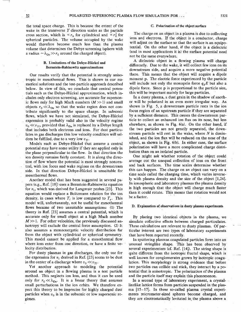
which approaches H in the limit 8 << 1. We have shown the effect of changing 8 in Fig. 7. Here we plot N and along the center line indicated in Fig. 2. From the figure we see only a small change in the solutions, as 8 is reduced from t to+· This test [with parameters from Fig. 4(b)] and tests on other parameters, shows that 8=t gives sufficient accuracy.

The second method is to multiply the ion loss term by a fudge factor {3 > 1. This gives

V·R r 1=-{3N--H(-V·R). R

(A14)

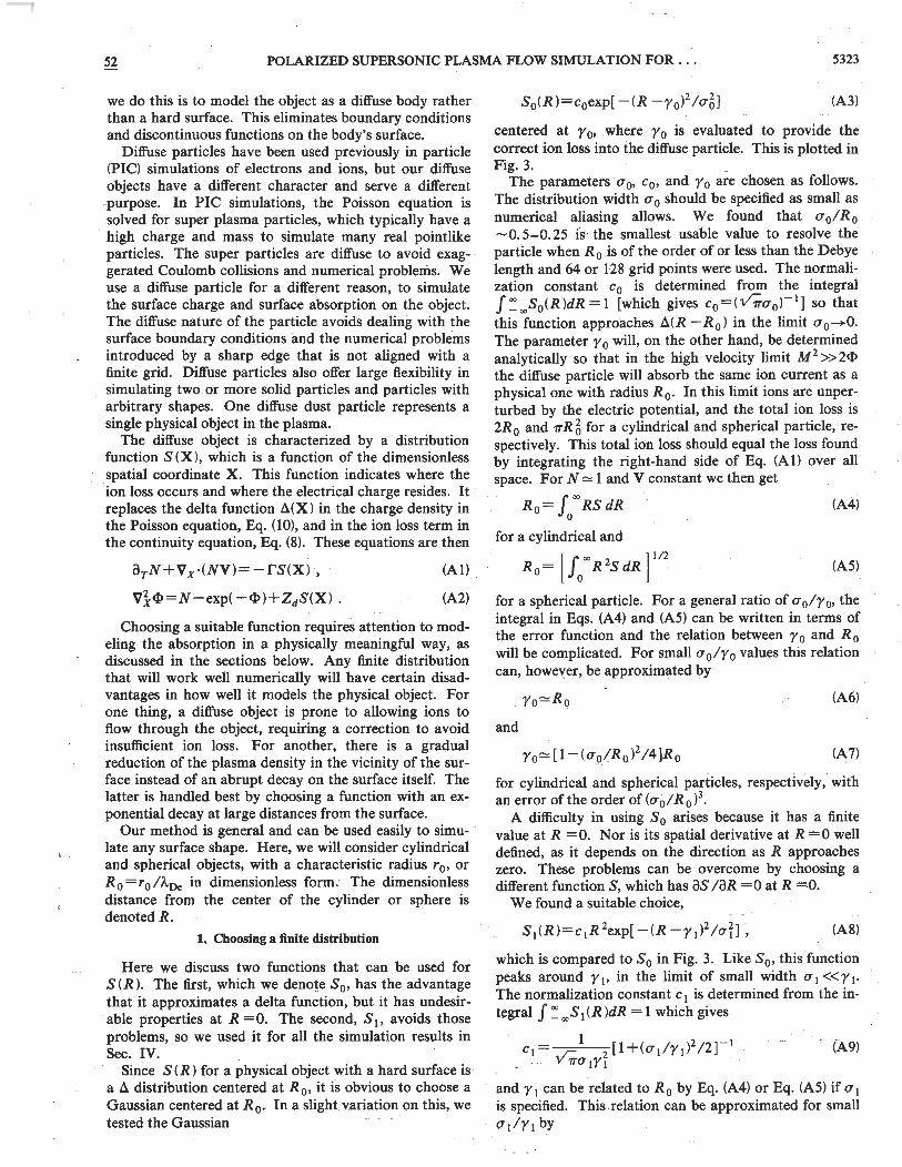
The constant {3 must be calibrated to a known expression for the ion loss. We chose {3 by running our simulation for M 2 >>2<1>, where we know that the cross section for ion absorption should be 1T R 6 for a sphere or 2R 0 for a cylinder. The ion loss is underestimated by a factor 1 /{3. This yields a value for {3, which we assume is valid for the lower Mach numbers for which our results are reported. To give an example of how the solution depends upon the choice of S and r, we have shown Nand along the center line in Fig. 8. Here we show numerical solutions for different S values [Eqs. (A3) and (A8)) and r values [Eqs. (A12) and (A14)] for the parameters used in Fig. 4(b).

8

(a) --o= 112 0

1:: 6 c

- - -o = 114 ---------0 = 118

II z ~ 'iii

4 1:: CD "0 1:: .Q 2

0

2 t-"' ~ 1.5 ....... -e-CD

--o= 112 -- -o= I/4 ---------o = 118

' II

e a; 0.5 E CD 0 0 c. <tS E gj -0.5 Ci

'2 Ro '

R object focal region

-1 0 4 8 12 16

distance X= x!Aoe

FIG. 7. Numerical test of the sensitivity of the simulation results to the parameter 8 in Eq. (Al3). This equation gives a smooth approximation of the Heavyside step function H in our numerical calculations. Equation (Al3) approaches H in the limit 8~0. Shown are Nand along the center line for three values of 8. The other parameters are the same as in Fig. 5(b).

0 1::

4

~- 3 II z ~ -~ 2 CD "0 1:: .Q

0

0

S- VARIATION

,:--.:\ I,'/~\ , l \. q ·. ,· "· ,I \ ' \ ; .. i ... I ~-/ \ . ~ I .

--s1 & rt --------s1 & ro ---·So & rt ---so & ro

i ~-i ~-- ~-/ '-I '-., i i . /

\ _,_: ·~.-.. .-:--··

4 8

distance X=xl A.09

12 16

FIG. 8. Numerical test of the sensitivity of the simulation results to the choice of functions for the diffuse object distribution Sand the ion flux r lost on the object. The functions S0 and S 1

are given by Eqs. (A3) and (A8), and r 0 and r 1 are given by Eq. (A12) and (Al4). Shown are Nand along the center line for the same parameters as Fig. 5(b).

APPENDIX B: NUMERICAL METHOD

Here we provide details of our numerical method of solving the system of fluid equations, which are Eqs. (8)-(10) with 11 replaced by S to define the diffuse object. We are interested in finding the steady-state solution. The boundary conditions are described earlier in this paper and are illustrated in Fig. 2. Recall that the flow enters a rectangular simulation box in the positive X direction. The boundary conditions are periodic in the directions transverse to the flow, and non periodic (Dirichlet and Neumann) on the inflow and outflow sides.

We carried out our simulations in 2D and 3D for an infinite cylindrical and a spherical object, respectively. The infinite cylinder is aligned perpendicular to the flow. The principles involved are the same for both geometries, so we shall give details below only for the 2D calculation.

The system of equations is solved by a spectral method where the solutions q (q =N, U, V, and ct>) are expanded in mx terms of Chebyshev (</J) and my terms of Fourier polynomials in the nonperiodic and periodic directions, respectively. The dimensions of the rectangular simulation box are [O,Lx] X [O,Ly ].

The solution procedure involves first a Fourier expansion of q

my/2-1

q(5, Y, T)= ~ ~k(5, T)exp(27TikY !Ly), (Bl) k= -my/2

where the Fourier coefficient ~ k ( 5, T) is a function of time T and a spatial coordinate 5, which is related to X by X=(Lx/2)(1+5). This new variable is introduced to map the X interval [O,Lx] into the interval [ -1, 1] normally used for the Chebyshev polynomials.

The Fourier coefficient is then expanded in terms of Chebyshev coefficients as

m"-1

~k(5,n= ~ i!j,k(r)rj(5), j=O

(B2)

where the expansion coefficients are assumed to be time dependent.

In the 5 (i.e., X) direction, q is found at the so-called Chebyshev-Gauss-Lobatto points [5j =cos( 7Tj lmx ), j =0, 1, . .. , mx ], which allow us to specify boundary conditions at both 5= -1 and 1. Gauss integration techniques can be used to obtain the expansion coefficients [26].

Expansion in terms of Chebyshev polynomials also allows us to use a fast-Fourier transform in the 5 direction, which gives an effective computation of the expansion coefficients for large mx and my values.

In order to obtain a stationary solution of the set of equation, Eqs. (8)-(10), it is necessary to add small diffusion (E 1 Vi Ni ) and viscosity terms (E2 Vi Vi ) to Eqs. (8) and (9), respectively. This is due to a nonlinear numerical effect, which after a finite time leads to unreasonably large gradients in the solution at the wake edge and at the ion focusing point behind the wake. To illustrate how the diffusion (E 1) and viscosity (E2) coefficients

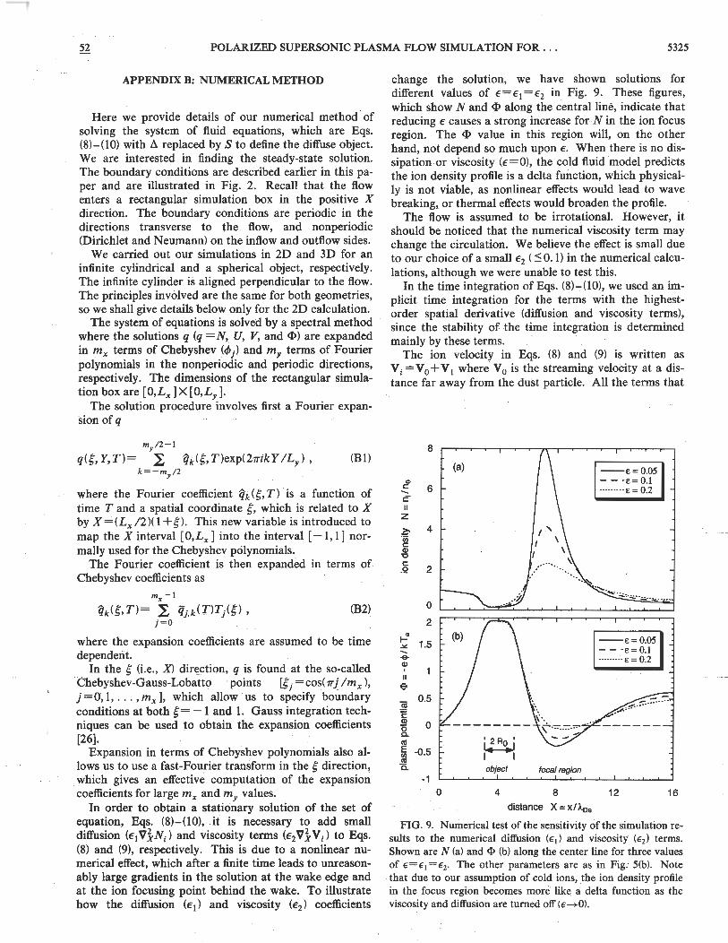
change the solution, we have shown solutions for different values of E=E1 =€2 in Fig. 9. These figures, which show N and ct> along the central line, indicate that reducing E causes a strong increase for N in the ion focus region. The ct> value in this region will, on the other hand, not depend so much upon E. When there is no dissipation or viscosity (E=O), the cold fluid model predicts the ion density profile is a delta function, which physically is not viable, as nonlinear effects would lead to wave breaking, or thermal effects would broaden the profile.

The flow is assumed to be irrotational. However, it should be noticed that the numerical viscosity term may change the circulation. We believe the effect is small due to our choice of a small E2 ( :S 0. 1) in the numerical calculations, although we were unable to test this.

In the time integration of Eqs. (8)-(10), we used an implicit time integration for the terms with the highestorder spatial derivative (diffusion and viscosity terms), since the stability of the time integration is determined mainly by these terms.

The ion velocity in Eqs. (8) and (9) is written as Vi= V 0 + V 1 where V 0 is the streaming velocity at a distance far away from the dust particle. All the terms that

8

0 c: 6 ,;;-II z ~ 4 "iii c: Q) "0 c: Q 2

0

2

~ 1.5 ~ ..... -&-Q) . II

e ~

0.5

E

* 0 a. al E -0.5 C/l al c.

-1

(a)

(b)

0

I 2 Ro I

R object focal region

4 8

distance X= x/A09

--e=0.05 -- -e=O.l ······ ···E=0.2

-~-""-·;.;.-;-:.:;_ •• :.:..··.!.:,..-····

--E=0.05 -- -e=O.l ·········E=0.2

12 16

FIG. 9. Numerical test of the sensitivity of the simulation results to the numerical diffusion (e-1) and viscosity (e-2 ) terms. Shown are N (a) and (b) along the center line for three values of e-=e-1 =e-2. The other parameters are as in Fig. 5(b). Note that due to our assumption of cold ions, the ion density profile in the focus region becomes more like a delta function as the viscosity and diffusion are turned off (E---+0).


involve V0 • V x are also integrated implicitly to improve stability for large M values.

The Poisson equation (10) is rewritten as a diffusionlike equation

The stationary solution of this equation will be identical to that of the Poisson equation.

Since we are mainly interested in finding the stationary solution of Eqs. (8)-(10) and not an accurate time integration, we used a time integrator with only a firstorder accuracy with respect to the time step !::..T. For the implicit and explicit terms we used forward and backward Euler integration, respectively.

After applying this time integration to the equations and applying a Fourier transform, the equations are reduced to a relation between the Fourier coefficients given by

Nn+ 1-itn k k +u _2_a ir+l

t::..T o L s k X

-E [_±_a2-k247T2 [Nn+l=fn (B4) I L1 s L2 k I '

X y

[1] J. Goree, Plasma Sources Sci. Techno!. 3, 400 (1994). [2] E. C. Whipple, Rep. Pro g. Phys. 44, 1198 ( 1981 ). [3] E. Coggiola and A. Soubeyran, J. Geophys. Res. A 5, 7613

(1991). [4] Ya. L. Al'pert, L. Gurevich, A. Quarteroni, and L. P. Pi

taevskii, Space Physics with Artificial Satellites (Consultants Bureau, New York, 1965).

[5] J. C. Taylor, Planet. Space Sci. 15, 155 (1967). [6] G. B. Murphy, D. L. Reasoner, A. Tribble, N. D'Angelo,

J. S. Pickett, and W. S. Kurth, J. Geophys. Res. 94, 6866 (1989).

[7] N.H. Stone, J. Plasma Phys. 26,351 (1981). [8] N.H. Stone, J. Plasma Phys. 26, 385 (1981). [9] R. L. Merlino and N. D'Angelo, J. Plasma Phys. 37, 185

(1987) . [10] S. J. Choi and M. J. Kushner, J. Appl. Phys. 75, 3351

(1994). [11] D. R. Nicholson, Introduction to Plasma Theory (John Wi

ley & Sons, New York, 1983). [12] P. K. Shukla, Phys. Plasma 1, 1 (1994). [13] P. Chenevier, J. M. Dolique, and H. Peres, J. Plasma

Phys. 10, 185 (1973). [14] G. Praburam and J. Goree, Astrophys. J. 441, 830 (1995).

(B6)

(B7)

where

L!=- ~ as[Nn(un-U0 )]+ay(NnVn)-rnS(X), X

and

The Chebyshev coefficients given in Eq. (B2) can be found from these equations by a method described in Dennis and Quartapelle [27] . This method involves transformation of Eqs. (B4)-(B7) to the Chebyshev space where it is shown (from the properties of the Chebyshev polynomials) that 'iJ.j,k can be found by solving a quasipentadiagonal matrix where the boundary conditions are imposed. For more details see Ref. [26] or [27].

[15] J. H. Chu and Lin I, Phys. Rev. Lett. 72, 4009 (1994). [16] Y. Hayashi and K. Tachibana, Jpn. J. Appl. Phys. 33,

L804 (1994). [17] J . B. Pieper, J . Goree, and R. Quinn (unpublished). [18] S. Hamaguchi and R. T. Farouki, Phys. Rev. E 49, 4430

(1994). [19] S. Hamaguchi and R. T. Farouki, Phys. Plasma 1, 2110

(1994). [20] L. D . Landau and E. M. Lifshitz, Fluid Mechanics (Per

gamon, Oxford, 1959). [21] 0 . Havnes, T. K . Aslaksen, and F. Melands0, J. Geophys.

Res. 95, 6581 (1990) . [22] J. Goree (unpublished). [23] I. Bernstein and I. Rabinowitz, Phys. Fluids 2, 112 (1959). [24] F. Melands0, T. Aslaksen, and 0. Havnes, Planet. Space

Sci. 41, 321 (1993). [25] S. V. Vladimirov and M. Nambu, Phys. Rev. E 52, 2172

(1995). [26] C. Canuto, M. Y. Hussaini, A. Quarteroni, and T. A.

Zang, Spectral Methods in Fluid Dynamics (Springer, New York, 1988).

[27] S. C. R. Dennis and L. Quartapelle, J. Comput. Phys. 61, 218 (1985).

Polarized supersonic plasma flow simulation for charged...

Documents

Transcript of Polarized supersonic plasma flow simulation for charged...