Polarization Analysis of a Balloon-Borne Solar … Analysis of a Balloon-Borne Solar Magnetograph...
57
Polarization Analysis of a Balloon-Borne Solar Magnetograph Final Report for NASA contract NAS8-38609 DoO 01 (NASA-CR-19390B) POLARIZATION ANALYSIS OF A BALLOON-BORNE SOLAR MAGNETOGRAPH Final Report (Alabama Univ.) 58 p N94-24852 Unclas G3/35 0206776 Daniel J Reiley Russell A Chipman (PI) Physics Department School of Science University of Alabama in Huntsville Huntsville, AL 35899 (205)895-6417x318 December 14, 1993 https://ntrs.nasa.gov/search.jsp?R=19940020379 2018-06-10T06:08:57+00:00Z
Transcript of Polarization Analysis of a Balloon-Borne Solar … Analysis of a Balloon-Borne Solar Magnetograph...

Polarization Analysis of a
Balloon-Borne Solar Magnetograph
Final Report for
NASA contract NAS8-38609 DoO 01
(NASA-CR-19390B) POLARIZATION
ANALYSIS OF A BALLOON-BORNE SOLAR
MAGNETOGRAPH Final Report (Alabama
Univ.) 58 p
N94-24852
Unclas
G3/35 0206776
Daniel J Reiley
Russell A Chipman (PI)
Physics Department
School of Science
University of Alabama in Huntsville
Huntsville, AL 35899
(205)895-6417x318
December 14, 1993
https://ntrs.nasa.gov/search.jsp?R=19940020379 2018-06-10T06:08:57+00:00Z
Table of Contents
Body of the report
The main text of the report contains the particular results of our
research which relate directly to the Experimental Vector Magnetograph
(EXVM) and the Balloon-borne Vector Magnetograph (BVM).
I. Abstract 2
II. Polarization 3
A brief overview of which elements in the EXVM and BVM are
relevant to this polarization analysis.
II1.Calculating the polarization errors 4
A polarization budget for the various surfaces in the BVM which
will allow the polarization specification to be met. A brief summary of
how to calculate the polarization aberrations.
IV. Specifying the Coatings 12
An explanation of the various coating specifications
V. Optical Design of the EXVM 18
Vl. Coating specification sheets for the BVM 28
Appendices
The appendices of this report contain the more general results of
our research on the general topic of polarization aberrations.
Appendix I. 41
A general discussion of polarization aberration theory, in terms of
the SAMEX solar magnetograph.
Appendix II. 42
Rigorous derivations for the Mueller matrices of optical systems.

I. Abstract
The ] O- 5 polarization specification for the Balloon-borne Vector Magnetograph
(BVM) can be met. The ] 0 - 5; specification is shown to be a limitation on the
diattenuation and retardance along the chief ray path through the optical system, such
that the magnitude of the polarization aberration piston term is constrained to be less
than .5' 1 O- S. Coating specification sheets are provided which will ensure that the
polarization sensitivity of the BVM will be less than
! O- 5. An optical design is provided for a vector magnetograph. Finally, to provide a
concrete mathematical meaning for polarization sensitivity, the polarization aberration
matrix is averaged of the exit pupil, showing that the coupling between circular and linear
states depends only on the magnitude of the polarization aberration piston term.
II. Polarization
Since our last meeting, we have completely re-calculated the polarization analysis
of the Balloon-borne Vector Magnetograph (BVM). This analysis reflects our deeper
understanding of the 1 O- s polarization specification, and includes improved polarization
specification sheets, which should allow cost savings analogous to the savings we
allowed by moving from custom lenses to catalog lenses.
• The mirrors and lenses in optical systems can change light's polarization state.
Since solar magnetographs operate by measuring the polarization state of the solar disc,
the effect of the mirrors and lenses on the polarization state must be well-characterized.
One way to characterize mirrors' and lenses polarization properties is to use
polarization aberration theory. Polarization aberration theory is applied to a previous
solar magnetograph design in the paper "Polarization analysis of the SAMEX solar
magnetograph," which is included in this report as Appendix I.
2

Since the polarimeter used in this system will be a rotating-retarder polarimeter, the
polarization state exiting the polarimeter will be constant. Therefore, the only optical
elements which will affect the accuracy of the solar magnetic field measurements will be
the polarization that is caused be the optics in front of the polarimeter.
This report includes specification sheets for coatings which are to be deposited on
the optical surfaces in front of the polarimeter. These specifications will not only ensure
that the system's polarization sensitivity will be less than 1O-5, but will also ensure that
these coatings can be procured economically. Because limits on the polarization are
rarely specified on coatings, vendors might only quote very expensive coatings.
The improved coating specification sheets eliminate this possibility because they
include example coatings which meet the polarization specification. These example
coatings are very simple, and should be very similar to stock coating designs which
vendors commonly use for applications which aren't polarization-critical.
Because the BVM must accurately measure the linear polarized components of the
light from the sum, the optics in front of the polarimeter must not couple circular
poiarization states into linear polarization states. The 1 O-5 polarization specification
then means that, for circularly polarized light input to the system, the degree of linear
polarization at any image point must be less than ] O- 5
For the simple example coatings described in the coating specification sheets, the
maximum degree of linear polarization in the light incident on the polarimeter is
0.78" 1o- 5 For these coatings, several other polarization errors which we could identify
are also small. When unpolarized light is incident, the maximum degree of polarization is
0.60 ] 0 -5. When perfectly polarized light is incident, the degree of polarization is
reduced by less than 0.01' ! 0-5.
III. Calculating the polarization errors
3

The theory behind the calculations on this instrument is called "Polarization
aberration theory," and is presented in detail in Appendix I. For this analysis, polarization
aberration theory was expanded to include the polarization aberration expansion in the
form of a Mueller matrix.
To understand polarization aberration theory, one must first understand how the
angle of incidence behaves at an interface. Figure 1 illustrates this behavior. The first
column represents the angle of incidence and the orientation of the plane of incidence.
The second column shows the geometry of the spherical wavefront incident on a
spherical surface. Figure lc shows the behavior of the angle of incidence for an on-axis
object point. The angle of incidence increases linearly from the center of the pupil, and
the orientation of the plane of incidence rotates twice around the pupil.
For off-axis object points, the geometry is still that of a spherical wavefront
intersecting a spherical interface. Therefore, the angle of incidence will have the same
form as the on-axis pattern. However, because the angle of incidence at the center of
the wavefront is not zero, the pattern will be displaced from the center of the pupil.
To understand polarization aberration theory, one must also understand coating
behavior at small angles of incidence. For small angles of incidence, both diattenuation
and retardance are well-approximated by a quadratic, and go to zero at normal
incidence.
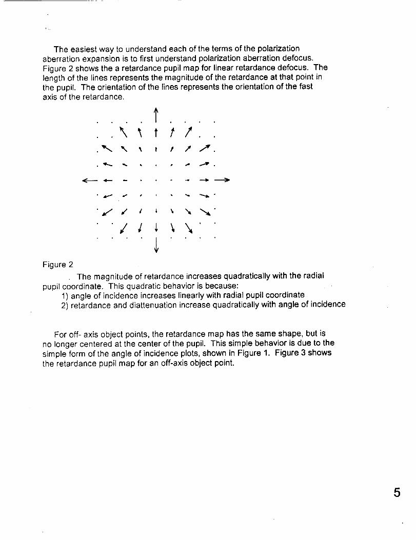
The easiest way to understand each of the terms of the polarizationaberration expansion is to first understand polarization aberration defocus.Figure 2 shows the a retardance pupil map for linear retardance defocus. Thelength of the lines represents the magnitude of the retardance at that point inthe pupil. The orientation of the lines represents the orientation of the fastaxis of the retardance.
t\ ttl
._.. \ _ t f ,," 7.
• _ q_. • , • _ _ .
• j # l _ ,, '_ "_"
Figure 2
The magnitude of retardance increases quadratically with the radialpupil coordinate. This quadratic behavior is because:
1) angle of incidence increases linearly with radial pupil coordinate2) retardance and diattenuation increase quadratically with angle of incidence
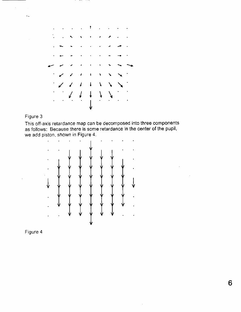
For off- axis object points, the retardance map has the same shape, but isno longer centered at the center of the pupil. This simple behavior is due to thesimple form of the angle of incidence plots, shown in Figure 1. Figure 3 showsthe retardance pupil map for an off-axis object point.
5
w
Figure 3
This off-axis retardance map can be decomposed into three components
as follows: Because there is some retardance in the center of the pupil,
we add piston, shown in Figure 4.
Figure 4
6
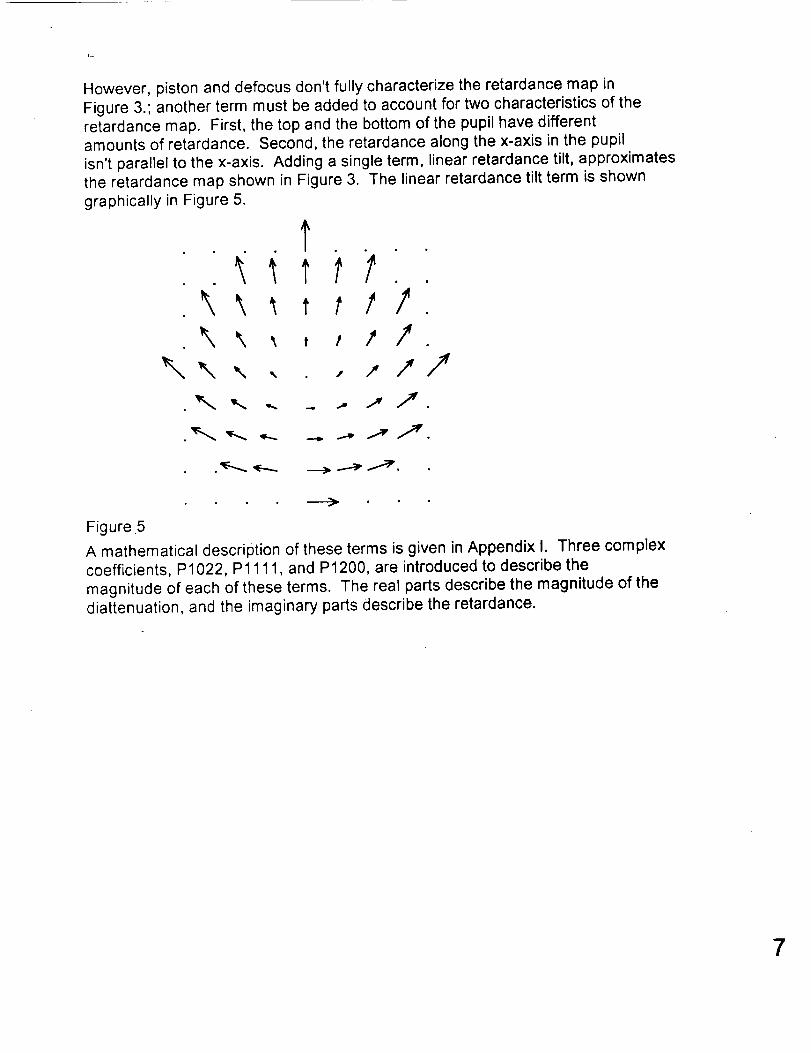
However, piston and defocus don't fully characterize the retardance map in
Figure 3.; another term must be added to account for two characteristics of theretardance map. First, the top and the bottom of the pupil have differentamounts of retardance. Second, the retardance along the x-axis in the pupil
isn't parallel to the x-axis. Adding a single term, linear retardance tilt, approximatesthe retardance map shown in Figure 3. The linear retardance tilt term is shown
graphically in Figure 5.
t
\ \ _ , i I /+\ ",,, ',, ,, , i 1,7
._,_.,,_ .,.... _.,, _ i_i _.
Figure 5
A mathematical description of these terms is given in Appendix I. Three complex
coefficients, P1022, P1111, and P1200, are introduced to describe the
magnitude of each of these terms. The real parts describe the magnitude of the
diattenuation, and the imaginary parts describe the retardance.
7


The polarization aberration coefficients depend on the angles of incidence for the
chief and marginal rays as well as the coatings on the various surfaces. With a tilted
secondary mirror, the angles of incidence on the relevant surfaces are listed in Table 1.
prefilter
primary mirror
secondary mirror
front surface of lens
inner surface of lens
back surface of lens
Angles of Incidence
(with secondary tilted .3 ° )
marginal ray chief ray
0° .16 °
3.6 ° .16 °
4.5 ° .3 °
2.3 ° 2.2 °
9.3 ° 4.7 °
6.5 ° 3.20
For tilted and decentered optical systems, such as the BVM with an articulating
secondary mirror, the meaning of the chief ray and the marginal ray are ambiguous. The
find the chief ray angle of incidence on each surface, we traced rays through the center
of the aperture stop to the center of the field of view and each edge of the field of view.
We called the maximum angle of incidence on that surface the chief ray angle of
incidence. This process was repeated for each of the relevant surfaces. A similar
process was used to find the marginal ray angles of incidence.
Most coating design programs give intensity reflection or transmission coefficients,
but the polarization aberration coefficients are defined in terms of amplitude reflection or
_CKDtNg PAGE BLANK NOT FILMED
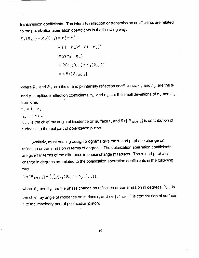
transmission coefficients. The intensity reflection or transmission coefficients are related
to the polarization aberration coefficients in the following way:
Rp(Oc._)- R,(Oc.,) = r 2p- r,2
= (l - qp)_- (l - q,)2
-= 2(q_ - qp)
=2(r,(e_,,)-rp(e_,,))
= 4Re[Pl2oo,,],
where R, and R p are the s- and p- intensity reflection coefficients, r _ and r p
and p- amplitude reflection coefficients, q, and q p are the small deviations of r, and r
from one,
11_ = ] - rs
q_, = I - rp
Oc., is the chief ray angle of incidence on surface i, and Re[ P 12oo. ,] is contribution of
surface L to the real part of polarization piston.
are the s-
Similarly, most coating design programs give the s- and p- phase change on
reflection or transmission in terms of degrees. The polarization aberration coefficients
are given in terms of the difference in phase change in radians. The s- and p- phase
change in degrees are related to the polarization aberration coefficients in the following
way:
] ft
lm[ P ,zoo.,] = 6p(e=.,)),
where 6 _ and 5 p are the phase change on reflection or transmission in degrees, e _. _ is
the chief ray angle of incidence on surface i, and Ira[ P _2oo. i] is contribution of surface
i to the imaginary part of polarization piston.
10

To find the total polarization piston for the system, use a coating program to
calculate R ,, R p, 6,, and 6 p for each surface at the angle of incidence for the chief ray
at that surface. Use the previous equations to find each surface's contribution to
polarization piston, .P _2oo.i. Add the contributions from each surface to find the total
polarization piston for the system:
P12oo = _ P12oo,i'
IV. Specifying the coatings
To ensure that the polarization sensitivity for the BVM is within the. 1 O- 5
specification, we suggest the polarization budget listed in Table 2. This polarization
budget, which is the basis for the coating specifications listed in Section VI, ensures that
the degree of linear polarization is less than ! O-s when circularly polarized light is
incident.
11

Prefilterfiltersideotherside
Primarymirror
Secondarymirror
Doub. (Front)
Doub. (int.)
(fixed)
Doub. (back)
Table2.
Polarization Piston Budget
0.005" 10 .5 <RePlzoo<0.04" ]0 -5
0.005" 10 -s <RoP,200<0.015 •|0 -s
0<ImP12oo<0.12. 10 -s
O<IrnP lzoo<0.02 • lO -s
-0.01" 10 -5 <RePlzoo<0 -0.07' 10 -s <ImP=zoo<-0.035" 10 -s
-0.025' 10 -s <RePlzoo<0 -0.16" 10 -s <IrnPIzoo<-0.1" 10 -5
0.35" lO -s <ReP 12oo<0.5" lO -s O<Im P izoo<0.005' 10 -s
Re P,2oo=0.08' ]0 -5 ImP Izoo=0
-0.83" lO "s <RePIzoo<-0.5' ]0 -s 0<irn p 1zoo<0.33. ]0 -s,
We also suggest that the mirrors have high reflectivity and the lens surfaces have
high transmission, greater than 98% over the entire range of relevant incident angles and
apertures.
Although we provide simple example coating designs which meet this specification,
we choose not to recommend coating designs with this report because the most
economical way to meet these specifications varies widely from vendor to vendor. Most
vendors have stock coating designs which will meet these specifications, and will not
need to charge for a coating design. To demonstrate the ease of designing coatings
which meet these requirements,
12

Table
Polarization Piston Terms:
Simple coatings
_ RePl2oo IrnP12oo
Pref. Front (LH)4(HL) 4 0.03' lO -s 0.10' lO -s
Pref. Back QWOT MgF 0.01" 10-5 0.0004" 10 -s
Primary HLHLAI -0.005' 10-S -0.04" 10 -5
Secondary HLHLAI -0.02' IO -s -0.12' lO -s
Doub. Front QWOT MgF 0.39' l O -s 0.002" 10 -s
Doub.int. 1 none 0.06" l O-S 0
Doub.lnt. 2 none 0.02" 10-S 0
Doub. Back 4 layer AR -0.79' l o-S 0.30" l O-S
SUM -0.30' 10- s 0.24:10 -s
The coatings should be specified to degrade the surface figure by less than X/10
RMS over the entire clear aperture, to prevent degradation of image quality. Surface
quality should be specified to meet MIL-SPEC 60-40 scratch-dig specifications; this is a
typical surface quality specification for scientific-grade optics. Surface durability should
be specified to meet the MIL-SPEC scotch tape test and eraser test; this is a fairly
stringent requirement, which is justified because this instrument will be used outdoors.
The following three pages describe the polarization errors graphically.
13

Diattenuation Vectors
In the image plane, the main polarization defect introduced by the coatings is thecoupling between linear and circular states caused by P1200
For a centered system (no tilted secondary), the diattenuation and retardancevectors are radially oriented in the image plane, with quadratically increasing
amplitude..
\ t / 7
For a tilted secondary, the diattenuation and retardance vectors have the samepattern, but are not centered in the center of the field. The exact location of thecenter depends on the coatings and amouont of tilt, but this figure isreasonable. For the specified coatings, the magnitude of the largest lineshown here is .8E-5.
Nasa2
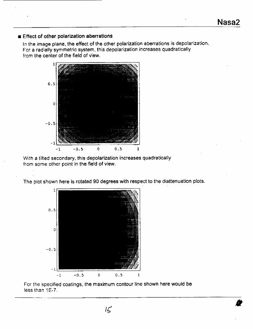
• Effect of other polarization aberrations
In the image plane, the effect of the other polarization aberrations is depo arization.
For a radially symmetric system, this depolarization increases quadraticallyfrom the center of the field of view.
0.5
-0.5
-i
-I -0.5 0 0.5 1
With a tilted secondary, this depolarization increases quadratically
from some other point in the field of view.
The plot shown here is rotated 90 degrees with respect to the diattenuation plots.
1
0.5
-0.5
-I
-i -0.5 0 0.5 1
For the specified coatings, the maximum contour line shown here would beless than 1E-7.
m

16
V. Optical design of the EXVM
While working on the polarization analysis of the NASA-designed instrument, we
noticed that it could be fabricated much more economically if catalog lenses were used
instead of custom lenses. After discussing the possibility with Mona Hagyard, Allen
Gary, and Ed West of NASA, we decided to redesign the optical system to take
advantage of these lenses.
Catalog lenses are lenses which are made for common optical tasks such as
collimating and focussing laser beams. Companies such as Melles-Griot, Spindler &
Hoyer, JML, Newport, Edmund, and CVI have dedicated large amounts of capital to
produce large numbers of commonly-requested focal lengths and diameters. Because
these lenses are made on a regular basis, they are much less expensive than custom
lenses of similar quality.
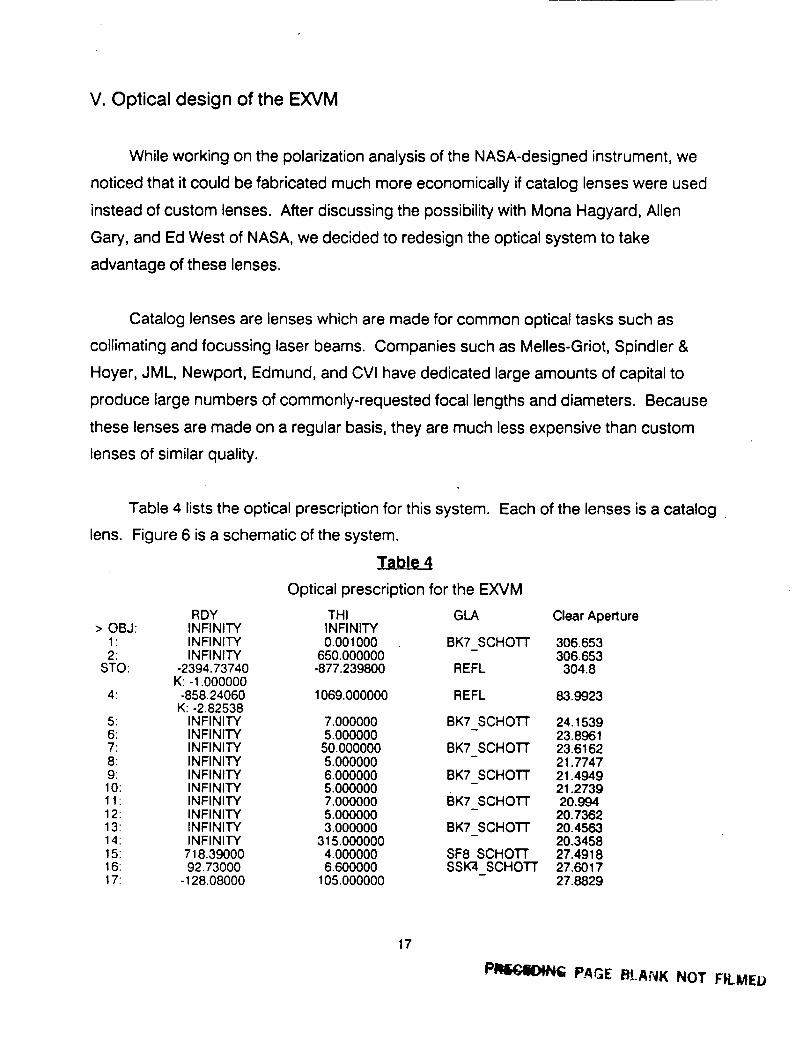
lens.
Table 4 lists the optical prescription for this system.
Figure 6 is a schematic of the system.
Each of the lenses is a catalog
Table 4
Optical prescription for the EXVM
RDY THI GLA Clear Aperture> OBJ: INFINITY INFINITY
1 INFINITY 0.001000 BK7 SCHOTI" 306.6532: INFINITY 650.000000 - 306.653
STO: -2394.73740 -877.239800 REFL 304.8K: -1.000000
4: -858.24060 1069.000000 REFL 83.9923K: -2.82538
5: INFINITY 7.000000 BK7 SCHOTI" 24.15396: INFINITY 5.000000 - 23.89617: INFINITY 50.000000 BK7 SCHOTT 23.61628: INFINITY 5.000000 - 21.77479: INFINITY 6.000000 BK7 SCHOTT 21.494910: INFINITY 5.000000 - 21.273911: INFINITY 7.000000 BK7 SCHOTT 20.99412: IN F IN ITY 5.000000 - 20.736213: INFINITY 3.000000 BK7 SCHO'I-r 20.456314: INFINITY 315.000000 - 20.345815: 718.39000 4.000000 SF8 SCHOI'I" 27.491816: 92.73000 6.600000 SSK-4 SCHOTr 27.601717: - 128.08000 105.000000 - 27.8829
17
PIqFI_;il)N_ PAGE BLANK NOT FILMEI_

18: INFINITY 300.00000019: INFINITY 33.50000020: 210.75000 5.00000021 : -81.29000 4.40000022: -515.63000 75.00000023: INFINITY -128.880000
ADE: 4524: 141.25000 -4.80000025: 47.31500 -3.00000026: -81.74800 - 15.00000027: INFINITY 0.01000028" INFINITY _8.00000029: INFINITY -4.00000030: INFINITY -48.00000031 : INFINITY 0.01000032: INFINITY -112.01700033: -188.36000 -12.50000034: 139.24000 _.00000035: 415.67000 -55.00000036: INFINITY 165.233309
ADE: 4537: INFINITY 4.00000038: INFINITY 12.00000039: INFINITY 21.00000040: INFINITY 0.00027541: . INFINITY 18.00000042: INFINITY 0.00000043: INFINITY 21.00000044: INFINITY 12.00000045: INFINITY 4.00000046: INFINITY 80.00000047: 673.17000 6.00000048: 222.27000 10.00000049: -302.87000 439.00000050: 121.71195 3.80000051 : -89.71796 2.50000052: -268.15906 131.02950653: 32.16000 4.46000054: -22.47000 1.50000055: -89.36000 34.92561156: INFINITY -120.845313
ADE: -1557: -182.72000 -2.00000058: -44.88000 -4.80000059: 64.04000 -72.00000060: INFINITY 257.078523
ADE: 1561: INFINITY -72.000000
ADE: 4562: INFINITY 108.000000
ADE: -45IMG: INFINITY 0.000000
SPECIFICATION DATAEPD 304.80000DIM MMWL 656.27
YAN 0.00000632.800.05717
BK7 SCHOTT
BAK4 SCHOI"rF3 SCHOTT
m
REFL
SF5 SCHOTTBKT-SCHOTT
BK7 SCHOTr
BK7 SCHOTT
BK7 SCHOTT
BK7 SCHOTTSF5-SCHOTT
REFL
BK7 SCHOTr
BK7 SCHOTT
BK7 SCHOTT
BK7 SCHOTr
BK7 SCHOTr
SF5 SCHOTTBKT-SCHOTT
BK7 SCHOTTSF5-SCHOTF
SK11 SCHOTTSF5 _CHOTT
REFL
SF5 SCHOTTSK1T SCHOTT
REFL
REFL
REFL
525.020.08167
20.922418.187620.462420.501520.566820.5172
20.431920.711220.765323.798923.797533.504934.037243.744643.743266.397266.553466.895566.142
63.878163.842
63.677663.7i363.71363.874463.874464.062664.226164.261965.351865.164565.129613.719913.280613.054717.997717.499117.42149.74839
16.800916.987917.600320.7726
32.0994
35.2717
40.0302
18

REFRACTIVEINDICESGLASS CODESSK4 SCHOTTSF8 S'CHOTTBAK"4 SCHO'I-rF3 SCHOTT8K"I SCHO'rFSF5-SCHOTFSKff SCHOTT
INFINITE CONJUGATESEFL -14063.1395BFL 109,3923FFL -0.3236E + 06FNO -46.1389IMG DIS 108.0000OAL 2301.9661PARAXlAL IMAGEHT 20.0458
ANG 0.0817EXIT PUPIL
DIA 13.2190THI -500.5187
656,271.6142661.6825051.5657611.6080631.5143231.6666121.561011
632.801.6153051.6844521.5667041.6095451.515O891.6684571.561883
525.021.6219231.69736213726951.61924413198671.6806661,567374
19

Figure 6: Schematic of the EXVM
EXVM - Solar Magnetograph
2O

Table 5 lists the first-order properties of the system. HMY is the height of themarginal ray, UMY is the slope of the marginal ray, HCY is the height of the chief ray, andUCY is the slope of the chief ray. A second representation of the system's first-orderproperties is in Figure 7, the y-y bar diagram of the system.
Eabte_5First-Order properties of the EXVM system
HMY UMY HCY UCYEP 152.400000 0.000000 0.000000 0.0014251 152.400000 0.000000 -0.926518 0.0009382 152.400000 0.000000 -0.9265 17 0.001425
STO 152.400000 0.127279 0.000000 -0,0014254 40.745715 -0.032327 1.250428 0.0043395 6.187768 -0.021270 5.889186 0.0028556 6.038879 -0.032327 5.909172 0.0043397 5.877242 -0.021270 5.930868 0.0028558 4.813749 -0.032327 6.073623 0.0043399 4.652112 -0.021270 6.095319 0.00285510 4.524493 -0.032327 6.112450 0.00433911 4. 362856 -0.021270 6.134146 0.00285512 4.213967 -0.032327 6.154132 0.00433913 4.052330 -0.021270 6.175829 0.00285514 3.988520 -0.032327 6.184394 0.00433915 -6.1 94598 -0.015503 7.551287 _ -0,00176216 -6.256610 -0.019362 7.544239 0.001 94017 -6.384400 -0.000403 7.557043 -0.03354818 -6.426724 -0.000265 4.034458 -0.02207319 -6.506265 -0.000403 -2.587524 -0.03354820 -6.519789 0.011009 -3.711396 -0.01491921 -6.464743 0.008406 -3.785991 -0.01582922 -6.427755 0.021331 -3.655639 -0.02100123 -4.827902 -0.021331 -5. 430683 0.02100124 -2.078715 -0.006732 -8.137238 0.03582725 -2. 046401 -0.012020 -8. 309207 0.02103826 -2.010341 -0.001344 -8. 372319 0.10246227 -1.990187 -0.000884 -9,909252 0.06741528 - 1.990196 -0.001344 -9. 908578 0.10246229 -1.925704 -0.000884 -14.826762 0.06741530 -1.9221 68 -0.001344 -15.096423 0.10246231 - 1.857677 -0. 000884 -20.014606 0.06741532 - 1.857685 -0.001344 -20.013932 0.10246233 -1.707182 -0.003984 -31.491437 0.01022934 -1.657381 -0.002464 -31.619301 0.03097735 -1.642596 -0.006831 -31.8051 63 -0.00001936 - 1. 266885 0.006831 -31. 804096 0. 00001937 -0.138158 0.004495 -31.800888 0.00001338 -0.120180 0.006831 -31.800837 0.00001939 -0.038206 0.004495 -31.800604 0.00001340 0. 056179 0. 006831 -31. 800336 0.00001941 0.056181 0. 004495 -31. 800336 0.00001342 0.137083 0.006831 -31.800106 0.00001943 0.137083 0.004495 -31.800106 0.00001344 0,231468 0.006831 -31.799838 0.00001945 0.313442 0.004495 -31.799605 0.00001346 0.331420 0.006831 -31.799554 0.00001947 0. 877909 0.003536 -31. 798001 0.01914248 0.899127 0.004338 -31.683148 0.00608649 0.942511 0.004976 -31.622263 0.063529
21

5O515253545556575859606162IMG
3.1270193.1060673.1018821.7015891.5857571.5565620.000000-5.385824-5.414985-5.5318904.751638-1.965719-1.185466-0.015O88
-0.005514-0.001674-0.010687-0.025971-0.019463-0.044568O.0445680.0145800.024355-0.0108370.010837-0,0106370.0108370.010637
-3.732943-3.534241-3.4254467.2972457.1 637757.1541484.874194
-3.014621-3.078942-3.268270-5.634672
-14.063994- 16.450397-20.000000
0.0522900.0435180.081834-0.029926-0.006418-0.0652800.0652800.0321600.0394430.032867-0.0328670.032867-0.032867-0.032867
22

Figure 7: y- y bar diagram of the EXVM.
160
-40 -30 -20
±
y bar
140
120
100
8O
6O
4O
__l
10
23

Table 6 lists the surface-by-surface third-order aberrations of the EXVM. SA standsfor spherical aberration, TCO stands for tangential coma, TAS stands for tangentialastigmatism, SAG stands for sa_gital astigmatism, PTB stands for Petzval blur, and DSTstands for distortion. All aberrations are in millimeters.
Iabte_6Third-order aberrations of the EXVM
SA TCO TAS SAG PTB DST1 0.000000 0.000000 0.000000 0.000000 0.000000 0.0000122 0.000000 0.000000 0.000000 0.000000 0.000000 -0.000012
STO 3.624628 -0.243555 0.003637 0.000000 -0.001818 0.000000-3.624628 0.000000 0.000000 0.000000 0.000000
4 -1.136824 0.123181 0.000625 0.003591 0.005074 -0.0001301.136776 0.104658 0.003212 0.001071 0.000033
5 -0.005470 0.002203 -0.000296 -0.000099 0.000000 0.0000136 0.005338 -0.002150 0.000289 0.000096 0.000000 -0.0000137 -0.005195 0.002092 -0.000281 -0.000094 0.000000 0.0000138 0.004255 -0.001714 0.000230 0.000077 0.000000 -0.0000109 -0.004112 0.001656 -0.000222 -0.000074 0.000000 0.00001010 0.004000 -0.001611 0.000216 0.000072 0.000000 -0.00001011 -0.003857 0.001553 -0.000208 -0.000069 0.000000 0.00000912 0.003725 -0.001500 0.000201 0.000067 0.000000 -0.00000913 -0.003582 0.001443 -0.000194 -0.000065 0.000000 0.00000914 0.003526 -0.001420 0.000191 0.000064 0.000000 -0.00000915 0.011116 -0.012094 0.005631 0.002707 0.001245 -0.00098216 -0.016057 0.046209 -0.044970 -0.015419 -0.000643 0.01479117 0.006307 -0.046646 0.093831 0.035623 0.006518 -0.06668018 0.000000 0.000003 0.000229 0.000076 0.000000 0.00634919 0.000000 -0.000003 -0.000232 -0.000077 0.000000 -0.00642820 0.002187 0.010711 0.021248 0.009591 0.003762 0.01565621 -0.010937 -0.011472 -0.004501 -0.001827 -0.000490 -0.00063922 0.005467 -0.006563 0.004241 0.002490 0.001615 -0.00099623 0.000000 0.000000 0.000000 0.000000 0.000000 0.00000024 -0.002159 -0.006579 -0.012924 -0.008470 -0.006243 -0.00860125 0.002601 0.021819 0.063919 0.023238 0.002897 0.06498926 -0.000593 -0.013574 -0.115584 -0.046569 -0.012061 -0.35515627 0.000000 0.000029 -0.002204 -0.000735 0.000000 0.05601628 0.000000 -0.000029 0,002204 0.000735 0.000000 -0.05601629 0.000000 0.000028 -0.002132 -0.000711 0.000000 0.05420130 0.000000 -0.000028 0.002128 0.000709 0.000000 -0.05410131 0.000000 0.000027 -0.002057 -0.000686 0.000000 0.05228632 0.000000 -0.000027 0.002057 0.000686 0.000000 -0.05228633 0.000006 0.000629 0.025908 0.011272 0.003954 0.39372634 -0.000052 -0.002109 -0.029773 -0.010581 -0.000984 -0.14442435 O.000047 O.O01O07 O,009266 O,004503 O.002121 O.03196236 0.000000 0.000000 0.000000 0.000000 0.000000 0.00000037 -01000001 0.00OO00 0.000000 0.000000 0.000000 0.O000O0
38 0.000001 0.000000 0.000000 0.000000 0.000000 0.00000039 0.000000 0.000000 0.000000 0.000000 0.000000 0.00000040 0.000000 0.000000 0.000000 0.000000 0.000000 0.00000041 0.000000 0.000000 0.000000 0.000000 0.000000 0.00000042 -0.000001 0.000000 0.000000 0.000000 0.000000 0.00000043 0.000001 0,000000 0.000000 0.000000 0.000000 0.00000044 -0. 000002 0. 000000 0. 000000 0. 000000 0. 000000 0. 00000045 0,000003 0.000000 0.000000 0.000000 0.000000 0.00000046 -0,000003 0.000000 0.000000 0.000000 0.000000 0.00000047 0.000013 -0.000221 0.002591 0.001737 0.001310 -0.01008048 -0.000005 0.000247 -0.004633 -0.001956 -0.000617 0.031830
24

495O515253545556575859606162
SUM
0.0000000.001168-0.0014030.0006870.000823-0.0083580.0091030.0000000.048899-0.0885850.0636280.0000000.0000000.000000
0.024479
-0.0000870.0037530.009618-0.00876O0.018O63-0.0905780.0640300.000000O. 162022-0.198O130.0356720.000000
' 0.0000000.000000
-0.038080
-0.0053470.010140-0.0234980.0405300.156585.0.3313610.1599990.000000O.183774
-0.1496270.0189740.0000000.0000000.000000
0.081811
-0.0001430.007459-0.0088510.0157020.068533-0.1132320.0599120.0000000.064475
-0.0512660.0145290.0000000.0000000.000000
0.068093
0.0024590.006119-0.0015280.0032880.024507
-0.0041670.0098680.0000000.004826-0.0020860.0123070.0000000.0000000°000000
0.061233
-0.01289200079920.020220
-0.0667550.501119-0.409025O.1404740.0000000.071211-0.0381990.0027150.0000000.0000000.000000
0.182185
25

•Figure 8: Wavefront aberrations of the EXVM in the final image plane.
(-FA;_ _. oo aF:__,':._: :,:-F,_
F I ELD _F i GHT0.50 , 0.50
{ . OB',7 °1
i
oo,o , \\
-0.50
/f
4 /
J, .,j/.i
-0,50
0.50
-0.50
0.50
0.00 AEL._,T ]:','E
fiELD HFTGFIT
[ O. 000 °1O. 50
e×','_
-0.50
OPTICAL PATH
7.
DIFFEREHCE (HAVES)
"LG
-0.50
1
I
---- 525.0 1'4M t
I
ORIGINAL PAGE IS
OF POOR QUALITY
Section VI - Coating specification sheets
These optical elements will be used in a solar vector magnetograph, whichmeasures the magnetic fields on the sun's surface by measuring the polarization stateacross the surface of the sun. This particular instrument is designed to makeextraordinarily accurate magnetic field measurements, and therefore, must makeextraordinarily accurate polarization measurements. To make these accuratepolarization measurements, the coatings must be specified to maintain the image'spolarization state very accurately.
The angles of incidence for this system are small, so the polarization associatedwith the surfaces will also tend to be small. The polarization specifications for thesecoatings are meant to ensure that the polarization of the system is small enough to meetits design goals.
The small values for the polarization specifications are justified for several reasons.First, the extreme accuracy of the final instrument would be able to detect any increasefrom these values. Second, since there are several optical elements in the system, thepolarization induced by each element must be small. Finally, although the values for thepolarization specification are small, simple coatings meet the specification.
The example coatings which are included with these specification sheets are meantonly as a guide to vendors. We expect vendors to find stock coatings which are moreappropriate than the example coatings.
27

Prefilter - filter side
diagram of blank
The coating design should meet specifications 1 and 2.
1. Average intensity transmittance - bandpass filter> % over entire diameter, incident angles 0° - .16 °
;k = 525nm
< % outside of nm bandpass, centered on ;_ =525nm
over entire diameter, incident angles 0° - .16 °
2. Polarizationa) Retardance
Retardance is defined as:
A- 8_-8p,
where 8 _ and 8 _ are the phase change on transmission for the s- and p- polarizations
The retardance specification is:0</k <0.00014 °
over entire clear aperture, incident angles 0 ° - .16°
X. = 525nm
b) Intensity DifferenceIntensity difference is defined as:_'Rp-R,,
where R, and R _) are the intensity transmission coefficients for s- and p- polarized light.
The intensity difference specification is:0.0000002 < _ < 0.0000016
over entire clear aperture, incident angles 0° -. 16°
;_ = 525nm
3. Coating thickness variationsThe coating should be deposited with a process which is known to not degrade
transmitted wavefronts by over ;_/5 at 525 nm.
28

4. Surface qualitymust meet MIL-SPEC60-40 scratch-dig specification over entire surface
5. Surface durabilitymust meet MIL-SPECscotch tape and eraser tests over entire surface
The following simple coating meets the polarization specifications. This coating design ismeant only as a guideline for the vendors. The vendors should have stock coatingswhich are more appropriate.
Example coating design:Bandpass filter 1LHLHLHLHHLHLHLHL1.5
where L represents a coating layer of MgF 2 (n = 1.3883) of a thickness equalto one-quarter wave optical path length at X. = 525nm, and where H represents a coatinglayer of ZnS (n = 2.375) of a thickness equal to one-quarter wave optical path length atX. =525nm.
This example coating design gives a retardance value of/k =0.00011 ° and an intensity
difference of _ =0.0000014.
29

Prefilter - backing side
diagram of blank
The coating design should meet specifications 1 and 2.
1. Average intensity transmittance - backing side of filter plate> 97% over entire diameter, incident angles 0° -. 16°X = 525nm
2. Polarization - must be met on each side of prefiltera) Retardance
Retardance is defined as:A-Ss-8 pl
where 8, and 8, are the phase change on transmission for the s- and p- polarizations
The retardance specification is:0 < A < 0.00002 °
over entire clear aperture, incident angles 0° - .16 °
X = 525nm
b) Intensity DifferenceIntensity difference is defined as:
_DE Rp- R,,
where R s and R p are the intensity transmission coefficients for s- and p- polarized light.
The intensity difference specification is:0.0000002 < _ < 0.0000005
over entire clear aperture, incident angles 0° -. 16°
X = 525nm
3. Coating thickness variationsThe coating should be deposited with a process which is known to not degrade
transmitted wavefronts by over X/5 at 525 nm.
4. Surface quality
30

must meet MIL-SPEC 60-40 scratch-dig specification over entire surface
5. Surface durabilitymust meet MIL-SPEC scotch tape and eraser tests over entire surface
A single layer of quarter wave optical thickness at X = 525nm of MgF2 (n = 1.3883)meets the polarization specification. This coating design is meant only as a guideline forthe vendors. The vendors should have stock coatings which are more appropriate. The
example coating design gives retardance of/k = 0.0000004 ° and intensity difference of
= 0.0000004.
31

Primary mirror
diagram of mirror
The coating design must meet specifications 1 and 2:
° Average intensity reflectivity> 98% over entire diameter, incident angles 0 ° - 3.8 °
= 525nm
.
a)Polarization - must be met on each side of prefilterRetardance
Retardance is defined as:
A - 6s- 6_, where
6 s and 6, are the phase change on reflection for the s- and p- polarizations
The retardance specificationis:-0.00008 ° < & < -0.00003 °
overentire clear ape_ure, incident angies 0° -.16 °
N = 525nm
b) Intensity DifferenceIntensity difference is defined as:
• _D---Rv-R_ '
where R_ and R _ are the intensity reflection coefficients for s- and p- polarized light.
Theintensity difference specificationis:-0.0000004 <ID < 0
over entire clear ape#ure, incident angles 0 ° -.16 °
= 525nm
3. Coating thickness variationsThe coating should be deposited with a process which is known to not degrade
transmitted wavefronts by over _,./5 at 525 rim.
4. Surface qualitymust meet MIL-SPEC 60-40 scratch-dig specification over entire surface
32
5. Surface durabilitymust meet MIL-SPEC scotch tape and eraser tests over entire surface
A simple four-layer reflection-enhancement coating (HLHL) meets thisspecification. L represents a coating layer of MgF2 (n = 1.3883) of a thickness equal toone-quarter wave optical path length at ;_ = 525nm, and H represents a coating layer ofZnS (n = 2.38) of a thickness equal to one-quarter wave optical path length at
= 525nm. This coating design is meant only as a guideline for the vendors. Thevendors can probably design a coating which is more appropriate.
The example coating design gives retardance of _ = -0.00004 ° and an intensity
difference of _ =-0.0000002.
33

Secondary mirror
diagram of mirror
The coating design must meet specifications 1 and 2:
, Average intensity reflectivity> 98% over entire diameter, incident angles 0° - 4.6 °
X = 525nm
.
a)Polarization - must be met on each side of prefilterRetardance
Retardance is defined as:
A - 6s- 5p, where
6, and 5, are the phase change on reflection for the s- and p- polarizations
The retardance specificationis:-0.00015 ° < & < 0
over entire clear ape_ure, incident angles 0° -0.3 °
X = 525nm
b) Intensity DifferenceIntensity difference is defined as:
_D - R_,- R,,
where R s and R p are the intensity reflection coefficients for s- and p- polarized light.
Theintensity difference specificationis:-0.000001 <_ < 0
overentire clear ape_ure, incidentangles 0° -0.3 °
X = 525nm
3. Coating thickness variationsThe coating should be deposited with a process which is known to not degrade
transmitted wavefronts by over X/5 at 525 nm.
4. Surface qualitymust meet MIL-SPEC 60-40 scratch-dig specification overentire surface
34
5. Surface durabilitymust meet MIL-SPEC scotch tape and eraser testsA simple four-layer reflection-enhancement coating (HLHL) meets this
specification. L represents a coating layer of index 1.3883 of a thickness equal to
one-quarter wave optical path length at ;_ = 525nm, and H represents a coating layer of
index 2.38 of a thickness equal to one-quarter wave optical path length at X = 525nm.This coating design is meant only as a guideline for the vendors. The vendors canprobably design a coating which is more appropriate.
The example coating design gives retardance of _ = -0.00014 ° and an intensity
difference of _ =-0.00000068.
35

Front doublet surface
diagram of lens
The coating designs for both the front and the back of the doublet must meetspecifications 1 and 2:
1. Average intensity transmittance<98% over entire diameter, incident angles 0° -2.2 °X = 525nm
2. Polarization - must be met on each side of prefiltera) Retardance
Retardance is defined as:
A - 5,- 5p, where
8, and 5, are the phase change on transmission for the s- and p- polarizations
The retardance specification is:0 < A < 0.00005 °
over entire clear aperture, incident angles 0° - 2.2 °X = 525nm
b) Intensity DifferenceIntensity difference is defined as:
© - Rp- Rs,
where R _ and R p are the intensity transmission coefficients for s- and p- polarized light.
The intensity difference specification is:0.000012 < _ < 0.000020
over entire clear aperture, incident angles 0 ° - 2.3 °X = 525nm
3. Coating thickness variationsThe coating should be deposited with a process which is known to not degrade
transmitted wavefronts by over X/5 at 525 nm.
4. Surface quality
36

must meet MIL-SPEC 60-40 scratch-dig specification over entire surface
5. Surface durabilitymust meet MIL-SPEC scotch tape and eraser tests
A simple coating consisting of a single, quarter wave of MgF 2 optical thickness at
X. = 525nm and index = 1.3883 meets specifications 1 and 2. This coating design is
meant only as a guideline for the vendors. The vendors can probably design a coatingwhich is more appropriate.
The example coating design gives retardance of/k = 0.00001 ° and an intensity
difference of _D = 0.000014.
37

Back doublet surface
diagram of lens
The coating designs for both the front and the back of the doublet must meetspecifications 1 and 2:
° Average intensity transmittance< 98% over entire diameter, incident angles 0 ° -2.2_ °
X = 525nm
.
a)Polarization - must be met on each side of prefilterRetardance
Retardance is defined as:
/k=5,-6 0 , where
6, and 6, are the phase change on transmission for the s- and p- polarizations
The retardance specification is:0 </k <0.00038 °
over entire clear aperture, incident angles 0 ° - 3.2 °
X = 525nm
b) Intensity DifferenceIntensity difference is defined as:
_D_ R_- R_,
where .R, and fi' _, are the intensity transmission coefficients for s- and p- polarized light.
The intensity difference specification is:-0.000033 < _ < -.000020
over entire clear aperture, incident angles 0 ° - 3.2 °
7_ = 525nm
3. Coating thickness variationsThe coating should be deposited with a process which is known to not degrade
transmitted wavefronts by over X/5 at 525 nm.
4. Surface quality
38

.
must meet MIL-SPEC 60-40 scratch-dig specification over entire surface
Surface durabilitymust meet MIL-SPEC scotch tape and eraser tests
The following 4-layer antireflection coating meets the polarization specification:
Layer # Optical Thickness Refractive Index1 (waves)0 .0000 1.6219 Glass1 .2500 1.4569 SiO22 .2500 1.6299 CeF33 .5000 2.3750 ZnS4 .2500 1.3881 MgF25 .0000 1.0000 Air
REF. WAVELENGTH= .5250 MICRONSDESIGN ANGLE = .0000 DEGREES
The examp!e coating design gives retardance of R p - R,
difference of 5, - 5 p = = 0.00034 ° .
= -0.000032 and an intensity
39

Appendix I. The paper "Polarization Analysis of the SAMEX SolarMagnetograph" contains both a good summary of polarization aberrationtheory and a good demonstration of polarization aberration analysis.
40

Appendix II. Polarization Aberrations of unresolved point spread functions
This section explicitly provides the mathematics behind the polarization
specification which was presented in the body of the report. First, we present the
reasoning for the derivation of the Mueller matrix averaged over the point spread
function. Next, we derive the average Mueller matrix for rotationally symmetric systems.
Then, we use this Mueller matrix to explore three possible explanations of the ] 0 - s
polarization specification in rotationally symmetric systems. Finally, we explain how the
result from rotationally symmetric systems can be generalized into a result for slightly
decentered systems, such as a vector magnetograph with an actuating secondary
mirror.
In many imaging situations, the point spread function that is formed by the
system's optics is smaller than the resolution of the system's readout. The EXVM is a
good example of this type of system; the pixels on the CCD array are about the same
size as the point spread function.
For this situation, the Stokes vector averaged over the point spread function is
equal to the pupil-averaged Stokes vector. This equality can be understood by
recognizing that the intensity in the pupil of any two orthogonal polarization states is the
same as the intensity of those polarization states in the image. For example, if a 90% of
the intensity in the pupil is y-polarized and 10% is x-polarized, the intensity distribution in
the image plane will also be 90% y-polarized and 10% x-polarized. The polarization state
changes across the pupil and also changes across the point spread function, but the
average Stokes vector will be the same.
This equality can also be derived. The Jones vector in the exit pupil is
41

E= Ey
The Stokes vector in the exit pupil is defined in terms of sums and differences in intensity
measurements,
-5: = I_-I_ :IE:E,.-E_E_
/ 2Re(E' Ey)'
IR--IL k2lm(E_Ey)
where I, Q, U. V are the Stokes vector elements, [ h is the intensity of the light which
would pass through a horizontal polarizer, 1 _ is the intensity of the light which would
pass through a vertical polarizer, l,s. is the intensity of the light which would pass
through a 45 ° polarizer, 1135. is the intensity of the light which would pass through a
135 ° polarizer, ! R is the intensity of light which would pass through a right circular
polarizer, and I L is the intensity which would pass through a left circular polarizer.
The pupil-averaged stokes vector is
<_ .(/_;_.- _;_, .I<_:_.-_;_,>,°,,,,I.I<E.E.>,,.,,,,-<',',>o°,,.,I,
\ X 2Im(E'_E.) J /,,.,., _k <2lrn(E:E.)>p,,,,,,.,/ _,. 2lm(<E'_E.>p.p,,) J
where the brackets represent
< f>,_,,,,,,= f fd_,
42

where _ is the pupil coordinate. The units are chosen such that the area of the pupil is
unity. E [. E,_ Is the intensity of the x-polarized light in the exit pupil. Since there are no
optical elements between the exit pupil and the image, there will be the same amount of
x-polarized light in the image plane. Therefore,
<E'_E,_>p,,p, = <E",,E',,>p,f,
where the primed quantities refer to the quantities in the image plane. Clearly, the same
relationship holds true for the y-polarized light:
<E_Ey>p,p,,= <E"yE y>p,f.
Since there is the same amount of light polarized both horizontally and vertically in the
exit pupil and in the image, the average of the first two elements in the Stokes vector are
equal in the pupil and the point spread function,
<[>pup_.t = </>psi
<Q>p.pil = <Q>p.!
Since the choice of horizontal and vertical is arbitrary, the same relationship holds true
for the third element in the Stokes vector,
</-)'>pupil = </-")'>psi"
Since the first three elements of the Stokes vector are equal, the fourth must be equal as
well,
<It> pup_,_ = <[?'>psf'
These equalities can also be derived rigorously using properties of the Fourier
transform. The relationship between the Jones vector in the pupil plane, E, and the
Jones vector in the image plane, E', is a Fourier transform,
Instead of explicitly using the x- and y- components of the electric field, we will derive the
more general case, for E _ E n, where both o_ and 13 can be either x or y. Multiplying
the Fourier transform for both components of the electric field yields
43

E';E'_ - f E;_ -'_"_;d_ / E_'_°_;a;"
_ f f E"E_,2.h.(p-O)cZ_d_ ,
Averaging over the point spread function yields
<E"aE'r_>ps ! - f E"_E'r_d-h
Rearranging the order of integration yields
<E'[,E',>p, l = f f f E'_E_e'2"_' ;dp'e-'2"_"dcthclp
- I T-' {7 { E'_Er,} }d-p
.. <E'_En>p,,p ..
Therefore,
<E'_Er_>p,,p,l = <E" E'_>p, f
Since (x and 13 can both be either x. or y, this proof explicitly shows that the Stokes
vector averaged over the exit pupil is equal to the Stokes vector averaged over the point
spread function.
44

Because the average Stokes vector in the point spread function is the same as the
average Stokes vector in the image, the average Mueller matrix in the point spread
function is the same as the average point spread function in the pupil. Qualitatively, this
equality is even easier to understand than the equality for the Stokes vector. Since there
are no polarizers, retarders, or depolarizers between the exit pupil and the image, the
Mueller matrix for propagation from the exit pupil to the image must be the identity
matrix.
This relationship can also be proven rigorously. Assuming a uniform input
polarization state, we can distribute the averages among the matrices in the following
way when we average over the point spread function.
<S>ps F = <MSin>ps F
: <j_>PsFSln
A similar relationship holds when we average over the pupil.
< S > p,,l,,t = < M S ,,, > pu_,_
: < _/_ > pupilS ,n
Since we have already proven that the Stokes vector averaged over the pupil is equal to
the Stokes vector over the point spread function (< S > pup,t = < S > psF ), we can equate
the previous two equations
<,_[> PSFS,n : <S> ps F : <S> pupL ! = <j_> pup_iS,n •
Therefore, the Mueller matrix averaged over the point spread function is equal to the
Mueller matrix averaged over the exit pupil,
<,'_1 > PSF "= <J_ > pupit"
45

The easiest way to find the pupil-averaged Mueller matrix, _ (h), is to begin with
the polarization aberration Jones matrix, J (p, _, h). This matrix will have different
forms depending on the symmetries of the system.
The polarization aberration expansion which we will begin with is the Jones matrix
for rotationally symmetric systems:
j(p, _,/l) = Poooo(;o + Pl200(:; I h 2
P_hp(cos_ - sin _(;2)
P 1o22P 2(cos 2(1)0 1 - sin 2_2),
The polarization aberration terms have both real and imaginary parts
P]_,._, = r'lxxx + lq]xxx
To convert this Jones matrix into a Mueller matrix, use the following relationships:
46

2M,,(p,_,h)-Jl_J,, + J'2_dz, + JlzJ,2
2M 12(P
2M13(P
2MI4(P,¢
2M21(P
2Mz2(P
2M23(p
2M24(P, @
2M3L(P
2M32(P
2 3.I 3_(P
2,_,la4(p, d?
2M4L(P,_
2M4z(p ,
2 3.,I 43 (P,
2 ,_f ._._( p , ¢
£b,h)--Ji,J,, + J'z,Jz, - Jiz J ,2
,,h) -J
h)-j(J
¢,h) ..J
¢,h) --J
-J
h)=j(J
_,h) =J
¢,h) =J
h)=j(J]
h)=j(J:
h)= j(J'2
h)= j(J'2
h) = j(J
+ J_2J2z
- J_2J22
]lJ 12 + J'21J22 + J]2J II + J'22J21
l,J ,2 + J'2, Jz2- Jl2J,, - J22J2,)
]lJ ll + J]zJ L2 - J'2tJ21 - J'zzJ22
II J ll + J22J22 - J21J21 - J:2J 12
i J2, + J'z,J,, + JlzJ22 + J'2zJ,z
J2, + J'2,J I1 - J:2J22- J'z2J ,2
J22 + J'2,d 12 + Jl2Jzl + J'22J,,
J22 +JzlJ12-J]zJz,-J'22Jtl)
J II + J'22Jlz- J:lJzl -- J12Jz2)
J,, + J;zJ22- J;,Jz,- J'22J,2)
J _z + J'22J II -- J_J22- J]2J2_)
_2J 11 + J i,J_2- J i_Jzl - Jz_J _2)
J rc represents the element from row r and column c in the Jones matrix. M rc
represents the element from row r and column c in the Mueller matrix. This
4?

transformation from the Jones calculus into the Mueller calculus can be found in several
references: E.L. O'Neil, Introduction to StatisticalOptics, (Addison Wesley, 1963), A.
Gerrard and J.M. Burch, Introduction to Matrix Methods in Optics, (Wiley, 1975).
A second, more succinct, method of transforming a Jones matrix into a Mueller
matrix uses the Kroneker product:
k4 - U(J ® J')U-
U is defined as
U I!oo:)0 0 l
1 l
-i 0
The Kroneker product of two 2X2 matrices is
ata2 alb2 b_a2 b_b2 1dl C2 d2 cla2 Clb2 dla2 dlb2
c_c2 c_d2 d_c2 d_d2
This formalism can be found in "Obtainment of the polarizing and retardation parameters
of a non-depolarizing optical system from the polar decomposition of its Mueller matrix,"
J. Gil, E. Bernabeu, Optik, vol. 76, no. 2, 1987.
Converting the polarization aberration Jones matrix into a Mueller matrix yields a
matrix which is so complicated that its form is not evident. However, by looking at the
resulting Mueller matrix for the various aberration terms, we can see the form of the
48

entire Mueller matrix. In the following analysis, we will use the polarization aberration
expansion for a rotationally symmetric system. The results from other types of systems,
such as a Cassegrain telescope with an articulating secondary mirror, can be inferred
from our results. We choose not to work with the polarization aberration expansion for a
decentered system because the math becomes so unwieldy that the benefits of the
added generality are more than outweighed by the difficulties of the added complexity.
The Mueller matrix for a system with only polarization defocus is
f p20000 + 2 4P |022P
2Poooo F 1022P 2 cos 2_- 2Poooo r_o22pzsin2
\ o
2 P oooor lo=zP2cos 2
2 cos4ttPoooo + P_o=2P 4
- P_o22P 4sin 4_
2 Pooooq 1022P2sin 2¢
- 2Poooor io=2p2sin 2_
p_o=zp4sin 4_2 2 4
Poooo-Pto=2P cos4_
2 Pooooq ,o22P=cos 24_
o- 2Pooooqto_zP 2sin 2_
_ 2Pooooq,o2_pZcos2_ "2 2 4Poooo- Ploz2P
As expected, this is the Mueller matrix for a retarder and diattenuator with orientation that
rotates at twice the angular pupil coordinate. The Mueller matrix for a system with only
polarization tilt is
I po2ooo + PIlllh2p 2
2Poooor llllhpcos_
- 2Poooo r,,,,hp sin d_
0
2Poooor ,,lthpcos_
Poooo+ P,,,lh2p2cos2qb
- p_llh2p2sin2¢
2Pooooql,=lhp sin
- 2Poooort,,,hpsin_
- p_,,th2p2sin2_
z h _ zPoooo-P,_,l, p cos2_
2 P ooooq , , , , hp cos dp
o)- 2Pooooq,,,thpsin¢_
- 2Pooooq,,,thpcos_
2 2p2Poooo+ P1,,,h
As expected, this is the Mueller matrix for a retarder and diattenuator oriented radially.
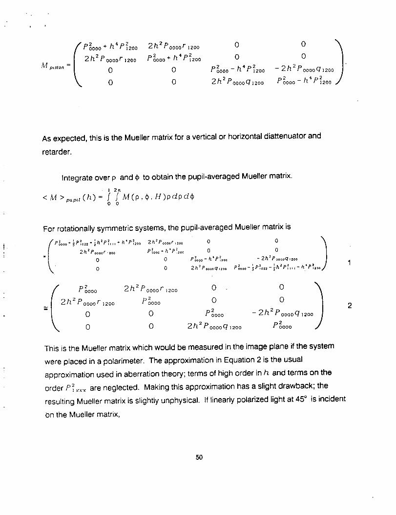
The Mueller matrix for a system with only polarization piston is
49
2 4 2
P + h P0000 1200
M p_,to_= _ 2 h 2 P !oo r 12oo
2h2p 00000 F 1200
p2 + h4 2oooo P l2oo 0
0 p2 _ h4p20000 1200
0 2_2 Pooooq 12oo
- 2h2pooooq,2oo
PLoo-.4Pf2ooY
As expected, this is the Muellermatrix for a ve_ical or horizontal dia_enuator and
retarder.
Integrate over p and _ to obtain the pupil-averaged Mueller matrix.
<M>I 2n.
p.p,t (h) = / f M(p,O,H)pdpdO0 0
For rotationally symmetric systems, the pupil-averaged Mueller matrix is
P2oooo _P,oz= _h P,,,i+h P,2oo 2h2Poooor,2oo2 4 2
2haPoooor_zoo . Poooo*h P_2oo 0 02 -- 4 20 0 Poooo h P_2oo -2hZPooo_q,zoo
• = , = , = 2 h.'P_=oo0 0 2h2Pooooq,zoo Poooo-;P,o=z-_h P_,,,-
I p2 2h2Poooo r ,200 0 0 1
0000
2h 2 P oooor 12oo P2oooo 0 0_ 2
0 0 P oooo - 2 h 2 p oooo q, 200
20 0 2 h 2 p oooo q, 200 P oooo
This is the Mueller matrix which would be measured in the image plane if the system
were placed in a polarimeter. The approximation in Equation 2 is the usual
approximation used in aberration theory; terms of high order in h and terms on the
order P_ _.,.,_are neglected. Making this approximation has a slight drawback; the
resulting Mueller matrix is slightly unphysical. If linearly polarized light at 45 ° is incident
on the Mueller matrix,
2
50

'_ln
the pupil-average stokes vector is
I P_oooo "_
2h2 eoooo F 12oo/S oo,= Po2ooo l'
/2 h 2p ooooq 12oo,,/
The degree of polarization for this Stokes vector is
DOP = ,_[Q2+ u2+ v21i
= 1 + 2h. 4 2P 1200
This Stokes vector is unphysical because the degree of polarization is greater than one.
This is not a serious problem, however, because, to be consistent with our previous
P _,.,(,(. In this case, the degree ofapproximations, we should drop terms of order 2
polarization for this Stokes vector is unity,
DOP = 1 .
Now that we have a pupil-averaged Mueller matrix, we can rigorously define three
polarization errors.
51

Polarization error #1 is that unpolarized light should not couple into polarized light.
The first effect of this polarization error is that magnetic field is measured when no
magnetic field is present. The second effect of this polarization error is that the
orientation of linearly polarized light is measured incorrectly, causing the orientation of
the magnetic field to be measured incorrectly. The symptom of this polarization error is
a spurious, radially oriented linear polarization with magnitude that increases
quadratically with field coordinate. Mathematically, this polarization error is
21Re(Pi2oo) l < 10 -s
We can investigate this polarization error more thoroughly using the Mueller
calculus. The Stokes vector for unpolarized light is
0
S= 0 "
0
When this unpolarized light is incident on the system, she Stokes vector averaged over
the exit pupil is
S I 21. Poooo
2 h-2 Poooo F 1200 .
0
O
This specification is a limit on the diattenuation along the chief ray. Numerically, this
polarization specification is
52

2 P oooor 1200 < 10 - s.
For the BVM with an articulating secondary mirror and a 30 cm. primary mirror with the
simple coatings listed in Table 3, the value for polarization error #1 is 0.60" ! O-S
Polarization error #2 is that polarized light should maintain its polarization state.
This specification would limit all off-diagonal elements in the pupil-averaged Mueller
matrix. One way to quantify this specification would be
21P12oo1< 10 -s.
This specification is essentially a limit on the diattenuation and retardance along the chief
ray path. This polarization error is the most important polarization error for the BVM
because it causes circularly polarized light to couple into linearlly polarized light.
Circularly polarized light has a Stokes vector of
0
S= 0 "
1
If this light is incident on an optical system, the pupil-averaged stokes vector in the image
plane is
S
E
p20000
2h. 2pooooF 12oo
- 2h2pooooq 12oo2
]D 0000
The degree of linear polarization for this Stokes vector is
53
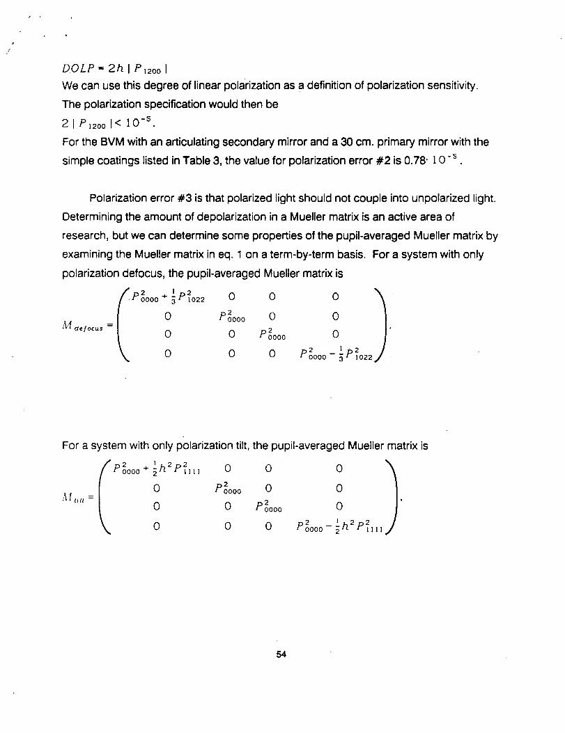
DOLP -- 2h I Pi2oo I
We can use this degree of linear polarization as a definition of polarization sensitivity.
The polarization specification would then be
21P]2oo1< 10 -5 .
For the BVM with an articulating secondary mirror and a 30 cm. primary mirror with the
simple coatings listed in Table 3, the value for polarization error #2 is 0.78' ] 0 -5
Polarization error #3 is that polarized light should not couple into unpolarized light.
Determining the amount of depolarization in a Mueller matrix is an active area of
research, but we can determine some properties of the pupil-averaged Mueller matrix by
examining the Mueller matrix in eq. 1 on a term-by-term basis. For a system with only
polarization defocus, the pupil-averaged Mueller matrix is
I 2 ÷1 2
Poooo 3 P'ozz
0
0
0
oo i 12Poooo 0
0 p20000
1 20 0 2 - _ P 1o22JD 0000
]_delocus
For a system with only polarization tilt, the pupil-averaged Mueller matrix is
/I. [_tilt
p2ooo + }h2p
0
0
0
2llll
o o o 1p2oooo 0 0
0 2Poooo 0
0 0 2 1Poooo - _h2 P_]ll
54
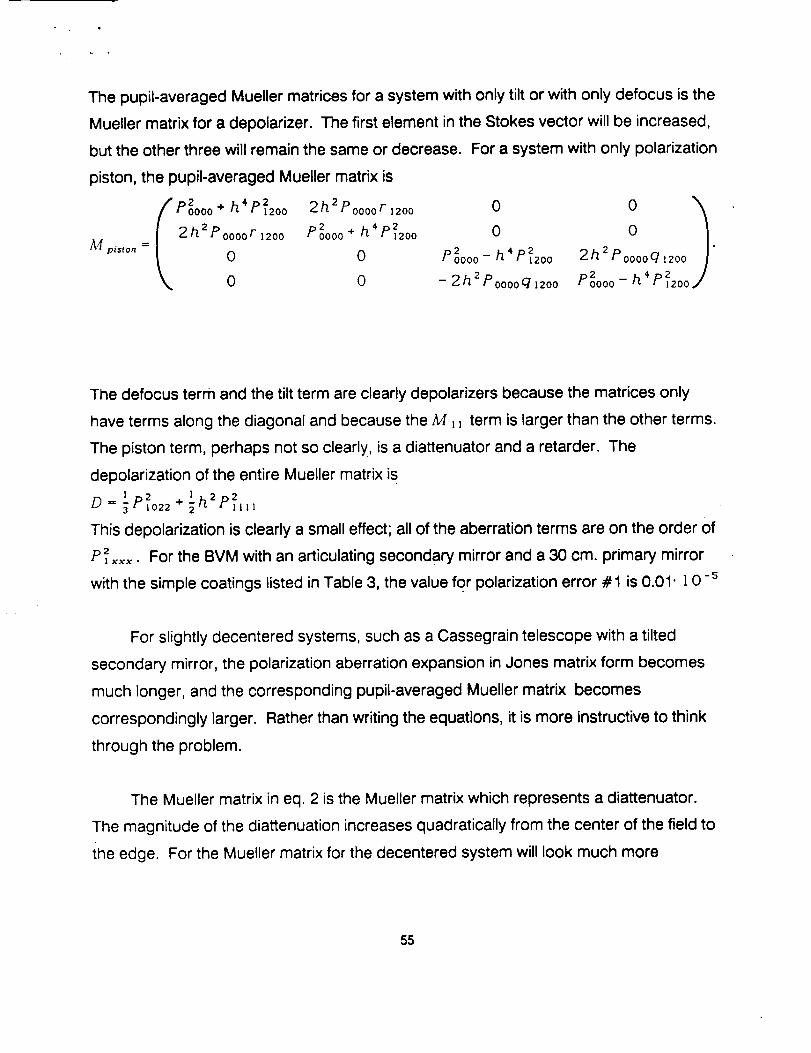
The pupil-averaged Mueller matrices for a system with only tilt or with only defocus is the
Mueller matrix for a depolarizer. The first element in the Stokes vector will be increased,
but the other three will remain the same or decrease. For a system with only polarization
piston, the pupil-averaged Mueller matrix is
i 2 h4 2
P oooo+ P 1200
2 h.2 Pooooc 12oo
M p_sto.= 0
0
2 h 2p oooor Izoo 0
pZ +h4p2 0000o 1200
0 p2 _h4p20000 I200
0 - 2hZPooooqlzoo
O)0
2 h 2 p oooo q 12oo
p2 h4p2_0000-- '_ J1200
The defocus term and the tilt term are clearly depolarizers because the matrices only
have terms along the diagonal and because the M 11 term is larger than the other terms.
The piston term, perhaps not so clearly, is a diattenuator and a retarder. The
depolarization of the entire Mueller matrix is
l 2 + _h2p2D = _P1o22 1ill
This depolarization is clearly a small effect; all of the aberration terms are on the order of
2P _,_,:,_. For the BVM with an articulating secondary mirror and a 30 cm. primary mirror
with the simple coatings listed in Table 3, the value for polarization error #1 is 0.01 • ] O-S
For slightly decentered systems, such as a Cassegrain telescope with a tilted
secondary mirror, the polarization aberration expansion in Jones matrix form becomes
much longer, and the corresponding pupil-averaged Mueller matrix becomes
correspondingly larger• Rather than writing the equations, it is more instructive to think
through the problem.
The Mueller matrix in eq. 2 is the Mueller matrix which represents a diattenuator.
The magnitude of the diattenuation increases quadratically from the center of the field to
the edge. For the Mueller matrix for the decentered system will look much more
55

complicated, but the meaning will be very similar. The orientation of the diattenuation will
be oriented radially about some non-axial image point, and the magnitude of the
diattenuation will increase quadratically from the same, non axial image point. Therefore,
we specified the coatings to meet the ] O-5 polarization specification at the most
extreme point in the image plane with a tilted secondary mirror.
56