Seminar

POLAR LIGHTS

Author: Ivana Novak

Mentor: prof. dr. Tomaz Zwitter

Presentation Dec 2010, Submitted Jul 2015

AbstractThis seminar presents phenomenon of polar lights, or aurorae. Magnetic field of the

Earth and its interaction with solar wind are described, as well as motion of chargedparticles in this field. Second part od seminar focuses on emission of light as a result ofcollisions between particles entering Earth’s atmosphere and molecules of atmosphere.Lastly, observational features of polar lights are presented.

Contents

1 Introduction 2

2 Geomagnetic field and Solar wind 32.1 Intrinsic magnetic field of the Earth . . . . . . . . . . . . . . . . . . . . . . . 32.2 Solar wind . . . . . . . . . . . . . . . . . . . . . . . . . . . . . . . . . . . . . 42.3 Interaction . . . . . . . . . . . . . . . . . . . . . . . . . . . . . . . . . . . . . 42.4 Van Allen radiation belts . . . . . . . . . . . . . . . . . . . . . . . . . . . . . 5

3 Magnetic mirroring and magnetic bottle 63.1 Escaping particles . . . . . . . . . . . . . . . . . . . . . . . . . . . . . . . . . 8

4 Appearance of aurora 84.1 Colour . . . . . . . . . . . . . . . . . . . . . . . . . . . . . . . . . . . . . . . 94.2 Form and dynamics . . . . . . . . . . . . . . . . . . . . . . . . . . . . . . . . 114.3 Proton aurora . . . . . . . . . . . . . . . . . . . . . . . . . . . . . . . . . . . 11

5 Auroral activity and prediction 12

1 Introduction

Polar lights (or aurorae polaris) are one of most spectacular atmospheric phenomena.Charged particles originating from solar wind manage to penetrate the Earth’s magneticshield and escape into upper atmosphere. There they excite molecules and atoms of the air.Result is a display of light, emitted by excited particles. It varies both in colour and shape.Auroras are most commonly green and red but also yellow, blue and purple, if they areintense enough. They can appear still or very dynamic, which depends on intensity of solarwind [1].They happen in ionosphere at the altitudes that can be as low as 80 km or as high as 600km. However, this is unusually high, top of the visible aurora commonly happens at 200-300km high.Auroras appear mainly in auroral zones. These are two ring-shaped regions around bothmagnetic poles with radius of approximatelly 2500 km around the pole. Thus they can beseen between 65 and 72 north and south latitudes. Aurora that is visible only from North-ern Hemisphere, is called aurora borealis or northern light, while in Southen Hemisphere itis called aurora australis or southern light [2].It is most easily observed from Scandinavia, Alaska and Canada during winter time whennights are long. If solar wind is especially strong it can be seen as low as St Petersburgor Scotland but these events are pretty rare. Southern lights are much less convenient toobserve from Earth since aurora has to be fairly strong before it can be seen from placesother than Antarctica. Tasmania or southern New Zealand have approximately the samechance to witness aurora as Scotland. Northern and southern light differ only in locationand are sometimes practically mirror images of one another.Best conditions for observing are on a clear dark night with no clouds or Moon. In winter

2

nights are much longer which also greatly improves chances. Aurora can be seen from duskto dawn, but most likely around midnight.

2 Geomagnetic field and Solar wind

Earth’s magnetic field is a compound of internal and external contributions.

~B = ∇(Φint + Φext)

In general we express planetary magnetic potential as infinite series using Legendre polyno-mials:

Φ = R

∞∑l=1

l∑m=0

[αlm

(Rr

)l+1

+ (1− αlm)(Rr

)]Plm(cos θ)[glm cosmφ+ hlm sinmφ]

Term α stands for magnetic field of internal sources while term 1 − α describes externalcontributions [3].Existence of a constant magnetic field that surrounds Earth is essential to life on the planet.It acts as a shield which deflects most of the charged particles planet is exposed to.

2.1 Intrinsic magnetic field of the Earth

In first approximation Earth’s magnetic field is described as dipole. In the sum above thedipole term is the one with l = 1. The axis of dipole differs from axis of terrestrial rotation- it is tilted by approximatelly 10.8. The relationship between magnetic and geographiccoordinates:

sinλM = sinλ sinλN + cosλ cosλN cos(φ− φN) sinφM =cosλ sin(φ− φN)

cosλM

Here λ = π/2− θ and N refers to North pole coordinates (its South Pole is near geographicNorth Pole (currently Ellesmere Island, North Canada) and its North Pole is in Adelie Land,French Antarctica. Next to that Earth’s rotation axis is also inclined 23.5 to ecliptic plane.As a result of Earth’s daily rotation and revolution, the angle between the line connectingSun and Earth and terrestrial magnetic dipole varies between about 56 and 90. Thisvariation importantly affects configuration of Earth’s magnetosphere.Magnetic field extends infinitely and weakens with distance, which effectivelly means severaltens of thousand kilometers into space. It forms Earth’s magnetosphere. Dipole aproximationis valid up to a few Earth radii where magnetic field significantly deviates from dipole becauseof interaction with the solar wind.

3

Figure 2: Dipole configuration of Earth’s magnetic field [4].

2.2 Solar wind

Solar atmosphere consists of four layers. The lowest is photosphere which emitts most ofthe sunlight. Next is chromosphere, followed by transition layer. The uppermost layer iscalled solar corona. It consists mostly of electrons, protons and light ions, such as Heliumnuclei, with density of about 7 particles per cm3. Solar wind is accelerated due to largepressure difference between the hot plasma at the base of corona and interstellar medium.The outflow is in part decelerated by solar gravity. This effect weakens with distance andis responsible for transition from subsonic to supersonic flow. At the point where it collideswith Earth’s magnetic field, speed of its flow is approximatelly 450km/s, proton temperatureis 1.2× 105K and electron temperature 1.3× 105K [1].

2.3 Interaction

At the distance of about 15 Earth radii Solar wind collides with the upper magnetosphere.Earth appears as an obstacle for solar wind flow. If plasma velocity was not too high, flowaround the Earth would proceed in an orderly, aerodynamic way. However, this is not the casein solar wind which is supersonic. In this case material that is deflected and has not actuallyreacted with obstacle, builds up an upstream, similar to a shock wave in front of a supersonicaircraft. This happens in a region called the bow shock, which marks the outer boundary ofthe magnetosphere. Within the bow shock the solar wind undergoes irreversible transitionduring which it is slowed down and heated up. After passing through the shock front thesolar wind is diverted around Earth in a region of turbulent motion called magnetosheat.The moving charged particles of the solar wind consistute electrical currents. They producean interplanetary magnetic field, which reinforces and compresses the geomagnetic field on

4

the day side and weakens and streches is on the night side. This results in the geomagnetictail, which extends far ”downwind” from the Earth. The transition between the deformedmagnetic field and the magnetosheath is called magnetopause [5].

Figure 3: Shape of Earth’s magnetosphere after being exposed to solar wind [4].

In such way two magnetic fields adapt to presence of one another. Their form depends ontheir strength - stronger field bends weaker field. It is obvious that solar wind and geomag-netic field don’t just balance in a form that we can see in Figure 3. Some charged particlesmust travel not along field lines but across them and somehow penetrate into Earth’s mag-netic field.This happens through process of magnetic reconnection (or magnetic merging). Several ex-isting magnetic field lines are cut if approached by oppositely pointing field lines. Theyabruptly short-circuit and the free ends are reconnected in other field lines. This is howtopology of magnetic field locally changes. Earth’s field is more stable than solar wind, soa chance for reconnection arises in two zones: at magnetopause and magnetotail. We callthis point X-point (or neutral point). At the center of X-point field magnitude is near zeroand field lines can merge. Plasma gets then transported toward neutral point while mergedfield lines are transported away. They are populated with mixed plasma coming from bothsources. As long as magnetic flux is transported toward the neutral point the reconnectionproces continues.The mechanism is very complicated and although first studies date back to 1950s and processhas been thouroughly dealt with, it is still poorly understood and scientists cannot agree onone model. This is why NASA launched Magnetospheric Multiscale Mission (MMS) in 2012.It consists of four spacecrafts that study Earth’s magnetosphere and will possibly explainthe process of reconnection.

2.4 Van Allen radiation belts

Charged particles that penetrate magnetosphere are trapped by the geomagnetic field linesand form Van Allen radiation belts [1]. They are in a shape of toruses and are held in placeby Earth’s magnetic field. The inner belt contains mainly protons, the outer belt energeticelectrons. The inner belt starts at about 1000 km above the Earth’s surface and extends to

5

an altitude of about 3000 km, while the outer belt occupies the region between 20000 and30000 km above Earth’s surface.

3 Magnetic mirroring and magnetic bottle

Once charged particle is trapped in Van Allen belts, its motion is prescribed by magnetic fieldof the Earth which we described earlier. Such configuration, where field strength changesas particle moves along a field line, is called magnetic mirroring effect [3]. It has been used,among other things, as a mean of plasma confinement, for example in fustion reactor [6].Van Allen belts act as a superposition of two such mirrors which is called magnetic bottle.The following derivation is taken from source [5]. In order to describe motion of the particle,we must introduce several new terms:

• smallness parameter rc/l, that describes the rate of change of field. If it is small,the field changes little during one gyration. Here rc is gyroradius, rc = v⊥

Ωcand l is

characteristic lenght of inhomogeneity

• gyroradius rg is radius of the circular path travelled by particle as it moves aroundmagnetic field line

• guiding center is the center of gyration

Trajectory of the particle is helix and can be decomposed to circular motion along the perime-ter of a circle with angular velocity Ωc and motion along the field line with aproximatelyconstant velocity v‖

~r − ~r0 =

axΩ2

cayΩ2

c∓ v⊥

Ωc

v‖t+ 12azt

2

+ rc

sin(Ωct− δ)±cos(Ωct− δ)

0

± ayt

Ω−caxtΩ−c0

This equation describes motion of particle in a uniform external field. First component is

due to accelerating motion of the guiding center along the magnetic field line, the second onedue to gyration around the guiding center with r′c and the third one appears because guidingcenter slowly drifts. It drifts because gyroradius slightly changes during one half-cycle ofparticle orbit (this happens because particle accelerates half of the cycle and deceleratesthe other half). Drift is caused because particle is affected by eternally perscribed field.It inevitably happens due to gravity but effect is negligible. It becomes important, whenparticle moves in nonuniform magnetic field, which will be our case.Magnetic field is not constant, but has some properties that simplify our equations: it variesslowly and its dominant component points to z direction. Therefore magnetic field changesvery little during one gyration, which we write mathematiccally as: rc

l 1. In cylindrical

coordinates:Br = Br(r, z), Bφ = 0, Bz = B0(z)

6

From this and ∇ · ~B = 0 we get Br = − r2(∂B0

∂z). We then solve equation of motion:vxvy

vz

=e

m

er eφ ezvr vφ vzBr 0 Bz

=eB0

m

vφ−vr

0

+er

2m

∂B0

∂z

0−vzvφ

We can see there are two contribution to accelerated motion of particle. First one is dueto gyration around large scale magnetic field and the second term represents slow spatialvariation of the field. From this equation it is obvious that particle drift is a slow processcompared to gyration.Radial component of velocity is vr = 0, while the other two are approximatelly constant(during a gyration). We can decompose velocity in parallel and perpendicular contributions,which are represented by z and φ components, respectively. If we average force that followsfrom equation of motion over φ, we get expression for parallel contribution of force, whichis also known as magnetic mirror force:

F‖ = mdv‖ds

= −µmdB

dsµm =

mv2‖

B

d

ds=

~B · ∇B

Quantity we encounter here is the magnetic moment µm, which is conserved as particle movesalong a magnetic field line into regions of stronger or weaker magnetic field (we measuredistance it travels with parameter s). Magnetic moment is one of adiabatic invariants whichare a powerful tool in explaining physics of space environment. We can show this fromexpression for total energy of a particle, which is conserved:

d

dt

(1

2mv2‖ +

1

2mv2⊥)

=d

dt

(1

2mv2‖ + µmB

)= 0,

therefore alsodµmdt

= 0

As gyrating particle moves in direction of increasing magnetic field, v⊥ must increase to keepµm constant, therefore v‖ must decrease. We must then reach the point where entire kineticenergy is converted to the perpendicular direction and particle can no longer move towardsregion of stronger field since that would violate conservation of energy. At this point particlehas no field-aligned velocity (v‖ = 0), while force F‖ = −µmdB/ds points in direction ofweaker field. Particle turns around and moves back toward diverging field lines.

Figure 4: Trajectroy of a particle trapped in Van Allen belts[4] .

7

Field distortion Trapped particles show diamagnetic behaviour and oppose magnetic fieldthat is deflecting them. This reduces magnetic field closer to the planet and strenghtens itat greater distances. For that reason field lines strech out. This distortion sets the limit tonumber of particles that can be trapped. On one hand we have fresh particles that enter thisclosed region and on the other hand those that get lost due to weakening field. Field is alsodistorted because electrons and ionst drift in the opposite directions (electrons to the eastand protons to the west), which creates ring current that also counters the original field.

3.1 Escaping particles

Since µm is conserved, variation of magnetic field is connected to variation of a pitch anglewhich is defined as angle between direction of magnetic field vector and particle velocityvector. Pitch angle equals 0 for a particle whose parallel motion is alonglocal magnetic fieldand 90 for a locally mirroring particle. It follows:

µm =1

2

mv2‖

~B=

1

2mv2 sin2 Θ

B= const. → sin2 Θ

B= const.

Let us assume magnetic field magnitude B0 and pitch angle Θ0 at reference point. If theparticle is moving towards region of increasing magnetic field magnitude, pitch angle varies:

sin2 Θ =B

B0

sin2 Θ0

At the mirror point pitch angle is Θm = π/2, therefore we can express field magnitudenecessary to reflect particle:

Bm =B0

sin2 Θ0

If the pitch angle is smaller, we need a larger magnetic field strength to reflect the particle.This means that under right circumstances particles can escape from Van Allen belts. Iftheir pitch angle is small enough, they will not be reflected. Instead, they will penetrate intoEarth’s upper atmosphere. We can define minimum angle for reflected particles for givenmagnetic field configuration with maximum magnetic field strenght Bmax:

sin2 Θmin =B0

Bmax

4 Appearance of aurora

Let us constrain ourselves for now to electrons since auroral images we are most familiarwith are associated with electron aurora.Once electrons penetrate into ionosphere, many things can happen. At some point they willcollide with molecules or atoms that constitute ionosphere. The more kinetic energy theyhave, the deeper can they penetrate and with depth increases also probability for collisions.Their energy is of several keV. But results of these collisions are light displays that vary incolour; it can be white, green, blue, violet or red. Some auroras appear inactive, while otherschange their characteristics (brightness, colour, position,...) very quickly.

8

4.1 Colour

Colour of polar light depends on several things: composition of atmosphere, its density andenergy of incoming electrons. It is determined by possible light emissions associated withspecific transitions between energy levels. General mechanism is simple and well-known.Electrons excite atoms and molecules in the air. When they return to ground (or otherlower level) state, they emit light. The colour of that light is determined by how muchenergy was released:

E = hν

Allowed lines are those that are produced via electric dipole transition. In general suchtransitions are associated with highest probability, as opposed to other possible transitionswhich are much less likely to happen. Electric dipole transitions are determined by selectionrules and produce the strongest spectral lines. Probability for transitions not approved byselection rules rises as we move to high atmosphere or outer space where we are dealingwith gases of extremelly low density or plasmas. When we reach the altitude of 500 km inionosphere, air density lowers from 1025 molecules per m−3 at sea level to 1012 molecules perm−3, which already presents conditions we are unable to achieve with any vacuum pump inlaboratory. Denisties in interplanetary space reach as low as 107 molecules per m−3. At suchlow densities collision between atoms are much less likely, which gives atoms more time toemit light and return to lower state. Since forbidden transitions take longer, from millisec-onds to seconds (while lifetimes of allowed states are of the order of microseconds or less),this provides ideal conditions for forbidden transitions.Tables 1 and 2 present some of the observed spectral lines.1 Data is derived from observa-tions done by several scientists mostly in the sixties, while more recent observations focuson detection of radiation in broader wavelenght range.

As we have established, colour distribution of aurora is determined by density of atmo-sphere. For every transition there is a corresponding characteristic time, needed for photonto be emitted. If this time is longer, atmosphere must not be too dense - mean free pathmust be long enough so that it corresponds to that time. Electrons with energy of severalkeV can reach as deep as 100-150 km. Dominant emissions here are a green line at 557.7nm and red line at 661.1 nm. First comes from excited oxygen and is caused by electricquadrupole transition 1D −1 S and is the cause of the most common appearance of aurora.Second one comes from excited nitrogen atoms. Electrons with less energy (around 1 keV)are stopped at higher altitudes (around 200 km). Here we find mostly oxygen atoms and theright conditions are met for emission of oxygen red line at wavelenght 630 nm. This line isparticularly interesting. It is emited by forbidden magnetic dipole transiton 3P −1 D of anatomic oxygen which takes almost two minutes (such transition is also responsible for redlines at 636.4 nm and 639.4 nm, although the last one is too weak to be observed). Whileits density decreases with altitude due to general exponential air density decrease, ratio ofatomic oxygen against other elements increases. Oxygen atoms can be excited at lower alti-tudes too, but photon with wavelenght of 630 nm will be emitted only if density is low. A

1Review of numerous observations and their results is done in the article: Vallance Jones A 1970 Auroralspectroscopy, published by Kluwer Academic Publishers. Both tables have been presented in the said article.

9

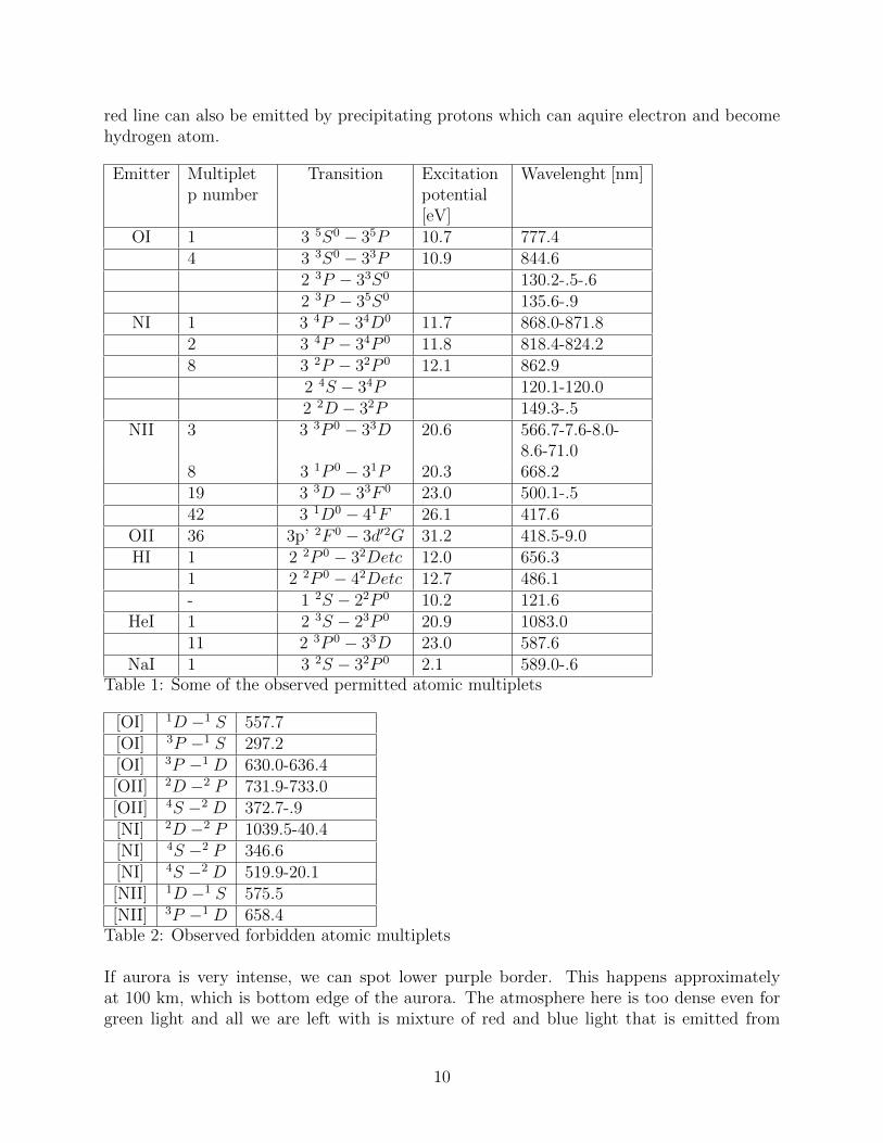
red line can also be emitted by precipitating protons which can aquire electron and becomehydrogen atom.

Emitter Multipletp number

Transition Excitationpotential[eV]

Wavelenght [nm]

OI 1 3 5S0 − 35P 10.7 777.44 3 3S0 − 33P 10.9 844.6

2 3P − 33S0 130.2-.5-.62 3P − 35S0 135.6-.9

NI 1 3 4P − 34D0 11.7 868.0-871.82 3 4P − 34P 0 11.8 818.4-824.28 3 2P − 32P 0 12.1 862.9

2 4S − 34P 120.1-120.02 2D − 32P 149.3-.5

NII 3 3 3P 0 − 33D 20.6 566.7-7.6-8.0-8.6-71.0

8 3 1P 0 − 31P 20.3 668.219 3 3D − 33F 0 23.0 500.1-.542 3 1D0 − 41F 26.1 417.6

OII 36 3p’ 2F 0 − 3d′2G 31.2 418.5-9.0HI 1 2 2P 0 − 32Detc 12.0 656.3

1 2 2P 0 − 42Detc 12.7 486.1- 1 2S − 22P 0 10.2 121.6

HeI 1 2 3S − 23P 0 20.9 1083.011 2 3P 0 − 33D 23.0 587.6

NaI 1 3 2S − 32P 0 2.1 589.0-.6Table 1: Some of the observed permitted atomic multiplets

[OI] 1D −1 S 557.7[OI] 3P −1 S 297.2[OI] 3P −1 D 630.0-636.4[OII] 2D −2 P 731.9-733.0[OII] 4S −2 D 372.7-.9[NI] 2D −2 P 1039.5-40.4[NI] 4S −2 P 346.6[NI] 4S −2 D 519.9-20.1[NII] 1D −1 S 575.5[NII] 3P −1 D 658.4

Table 2: Observed forbidden atomic multiplets

If aurora is very intense, we can spot lower purple border. This happens approximatelyat 100 km, which is bottom edge of the aurora. The atmosphere here is too dense even forgreen light and all we are left with is mixture of red and blue light that is emitted from

10

nitrogen atoms.Red aurora at high latitudes can be very bright. But because it is at the limit of visiblespectrum, we can barely see it with naked eye. Optical detectors have a better sensitivityto red colour which is why we can see so much red light in photographs of aurora.

4.2 Form and dynamics

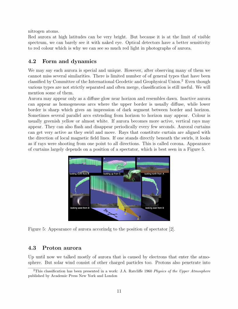
We may say each aurora is special and unique. However, after observing many of them wecannot miss several similarities. There is limited number of of general types that have beenclassified by Committee of the International Geodetic and Geophysical Union.2 Even thoughvarious types are not strictly separated and often merge, classification is still useful. We willmention some of them.Aurora may appear only as a diffuse glow near horizon and resembles dawn. Inactive auroracan appear as homogeneous arcs where the upper border is usually diffuse, while lowerborder is sharp which gives an impression of dark segment between border and horizon.Sometimes several parallel arcs extending from horizon to horizon may appear. Colour isusually greenish yellow or almost white. If aurora becomes more active, vertical rays mayappear. They can also flash and disappear periodically every few seconds. Auroral curtainscan get very active as they swirl and move. Rays that constitute curtain are aligned withthe direction of local magnetic field lines. If one stands directly beneath the swirls, it looksas if rays were shooting from one point to all directions. This is called corona. Appearanceof curtains largely depends on a position of a spectator, which is best seen in a Figure 5.

Figure 5: Appearance of aurora accorindg to the position of spectator [2].

4.3 Proton aurora

Up until now we talked mostly of aurora that is caused by electrons that enter the atmo-sphere. But solar wind consist of other charged particles too. Protons also penetrate into

2This classification has been presented in a work: J.A. Ratcliffe 1960 Physics of the Upper Atmospherepublished by Academic Press New York and London

11

atmosphere and collide with molecules. Their motion is equally restricted by magnetic fieldas those of electrons. However, when protons collide with molecules or atoms in the air,they are most likely to catch and electron from other particle and become hydrogen atom.Because this atom is now neutral, it can travel into any direction. In may turn into protonagain in the next collision or excite some other molecule. Process can repeat until protonsinitial energy is spent. Because its path is very irregular and not dictated by magnetic field,glow of proton aurora is very diffuse and usually not bright enough to be visible to humaneye.

5 Auroral activity and prediction

Probability for appearance of aurora is connected to solar activity. If solar wind is relativellycalm, aurora can be seen only as faint and at very high geographic latitudes. Sometimes,large disturbances in magnetosphere can occur. They are usually caused by variations in solarwind. Solar wind can be most severly perturbed during the peak solar activity when coronalmass ejections and solar flares are most frequent. Solar activity is periodic with severalperiods, most interesting is 11-year cycle. Still, some fluctuations can be completely random.This regularity in behaviour can be used to predict aurora to some extent. Such predictionsare aided by nearly real time data, provided by Solar and Heliospheric Observatory (SOHO),launched by NASA.

References

[1] Ian Ridpath: Oxford Dictionary of Astronomy, Oxford University Press, 2012

[2] Wikipedia, https://en.wikipedia.org/wiki/Aurora, accessed 30.6.2015

[3] Peter Prelovsek: Geofizika Univerza v Ljubljani, Fakulteta za matematiko in fiziko.

[4] W. Lowrie: Fundamentals of Geophysics. Cambridge University Press, 2007, ISBN: 13978-0-521-85902-8

[5] Tamas I. Gombosi: Physics of the Space Environment. Cambridge University Press,1998, ISBN: 0521 59264-X

[6] Wikipedia, https://en.wikipedia.org/wiki/Magnetic mirror, accessed 29.6.2015

[7] J. A. Ratcliffe: Physics of the Upper Atmosphere. Academic Press New York and Lon-don, 1960

[8] Duncan Bryant Electron acceleration in aurora and beyond. Institute of Physics Pub-lishing, 1998, ISBN: 07503 0533 9

[9] Atmospheric Optics; www.atoptics.com

12