Poisson traces, D-modules, and symplectic resolutions · The main technique is the study of a...
46
Lett Math Phys (2018) 108:633–678 https://doi.org/10.1007/s11005-017-1024-1 Poisson traces, D-modules, and symplectic resolutions Pavel Etingof 1 · Travis Schedler 2 Received: 30 April 2017 / Revised: 25 October 2017 / Accepted: 26 October 2017 / Published online: 5 December 2017 © The Author(s) 2017. This article is an open access publication Abstract We survey the theory of Poisson traces (or zeroth Poisson homology) devel- oped by the authors in a series of recent papers. The goal is to understand this subtle invariant of (singular) Poisson varieties, conditions for it to be finite-dimensional, its relationship to the geometry and topology of symplectic resolutions, and its appli- cations to quantizations. The main technique is the study of a canonical D-module on the variety. In the case the variety has finitely many symplectic leaves (such as for symplectic singularities and Hamiltonian reductions of symplectic vector spaces by reductive groups), the D-module is holonomic, and hence, the space of Poisson traces is finite-dimensional. As an application, there are finitely many irreducible finite-dimensional representations of every quantization of the variety. Conjecturally, the D-module is the pushforward of the canonical D-module under every symplectic resolution of singularities, which implies that the space of Poisson traces is dual to the top cohomology of the resolution. We explain many examples where the conjecture is proved, such as symmetric powers of du Val singularities and symplectic surfaces and Slodowy slices in the nilpotent cone of a semisimple Lie algebra. We compute the D-module in the case of surfaces with isolated singularities and show it is not always semisimple. We also explain generalizations to arbitrary Lie algebras of vector fields, connections to the Bernstein–Sato polynomial, relations to two-variable spe- cial polynomials such as Kostka polynomials and Tutte polynomials, and a conjectural B Travis Schedler [email protected] Pavel Etingof [email protected] 1 Massachusetts Institute of Technology, Cambridge, MA, USA 2 Imperial College London, London, UK 123
-
Upload
nguyenkhanh -
Category
Documents
-
view
223 -
download
0
Transcript of Poisson traces, D-modules, and symplectic resolutions · The main technique is the study of a...

Lett Math Phys (2018) 108:633–678https://doi.org/10.1007/s11005-017-1024-1
Poisson traces, D-modules, and symplectic resolutions
Pavel Etingof1 · Travis Schedler2
Received: 30 April 2017 / Revised: 25 October 2017 / Accepted: 26 October 2017 /Published online: 5 December 2017© The Author(s) 2017. This article is an open access publication
Abstract We survey the theory of Poisson traces (or zeroth Poisson homology) devel-oped by the authors in a series of recent papers. The goal is to understand this subtleinvariant of (singular) Poisson varieties, conditions for it to be finite-dimensional, itsrelationship to the geometry and topology of symplectic resolutions, and its appli-cations to quantizations. The main technique is the study of a canonical D-moduleon the variety. In the case the variety has finitely many symplectic leaves (such asfor symplectic singularities and Hamiltonian reductions of symplectic vector spacesby reductive groups), the D-module is holonomic, and hence, the space of Poissontraces is finite-dimensional. As an application, there are finitely many irreduciblefinite-dimensional representations of every quantization of the variety. Conjecturally,the D-module is the pushforward of the canonical D-module under every symplecticresolution of singularities, which implies that the space of Poisson traces is dual to thetop cohomology of the resolution. We explain many examples where the conjectureis proved, such as symmetric powers of du Val singularities and symplectic surfacesand Slodowy slices in the nilpotent cone of a semisimple Lie algebra. We computethe D-module in the case of surfaces with isolated singularities and show it is notalways semisimple. We also explain generalizations to arbitrary Lie algebras of vectorfields, connections to the Bernstein–Sato polynomial, relations to two-variable spe-cial polynomials such as Kostka polynomials and Tutte polynomials, and a conjectural
B Travis [email protected]
Pavel [email protected]
1 Massachusetts Institute of Technology, Cambridge, MA, USA
2 Imperial College London, London, UK
123

634 P. Etingof, T. Schedler
relationship with deformations of symplectic resolutions. In the appendix we give abrief recollection of the theory of D-modules on singular varieties that we require.
Keywords Hamiltonian flow ·Complete intersections ·Milnor number ·D-modules ·Poisson homology · Poisson varieties · Poisson homology · Poisson traces · Milnorfibration · Calabi–Yau varieties · Deformation quantization · Kostka polynomials ·Symplectic resolutions · Twistor deformations
Mathematics Subject Classification 14F10 · 37J05 · 32S20 · 53D55
1 Introduction
1.1. This paper gives an introduction to the theory of traces on Poisson algebrasdeveloped by the authors in a series of recent papers [13,14,20,22–25,50]. It is basedon two minicourses given by the authors at Cargese (2014) and ETH Zurich (2016).
Let A be a Poisson algebra over C, for example, A = O(X), where X is an affinePoisson variety. A Poisson trace on A is a linear functional A→ C which annihilates{A, A}, i.e., a Lie algebra character of A. The space of such traces is the dual,HP0(A)∗,to the zeroth Poisson homology, HP0(A) := A/{A, A}, the abelianization of A as aLie algebra (where {A, A} denotes theC-linear span of Poisson brackets of functions).
The space HP0(A) is an important but subtle invariant of A. For example, it is anontrivial questionwhenHP0(A) is finite dimensional. Indeed, even in the simple caseA = O(V )G , where V is a symplectic vector space and G a finite group of symplectictransformations of V , finite dimensionality of HP0(A) used to be a conjecture due toAlev and Farkas [1]. It is even harder to find or estimate the dimension of HP0(A);this is, in general, unknown even for A = O(V )G .
The first main result of the paper is a wide generalization of the Alev–Farkasconjecture, stating that HP0(A) is finite dimensional if X := Spec A is a Poissonvariety (or,more generally, scheme of finite type)with finitelymany symplectic leaves.Namely, the Alev–Farkas conjecture is obtained in the special case X = V/G. Amore general example is X = Y/G where Y is an affine symplectic variety, and G isa finite group of automorphisms of Y (such as symmetric powers of affine symplecticvarieties). But there are many other examples, such as Hamiltonian reductions ofsymplectic vector spaces by reductive groups acting linearly and affine symplecticsingularities (which includes nilpotent cones and Slodowy slices, hypertoric varieties).This result can be applied to show that any quantization of such a variety has finitelymany irreducible finite-dimensional representations (at most dimHP0(O(X))).
The proof of this result is based on the theory of D-modules (as founded in 1970–1971 by Bernstein and Kashiwara in, e.g., [7,41]). Namely, we define a canonicalD-module on X , denoted M(X), such that HP0(O(X)) is the underived direct imageH0π∗M(X) under the map π : X → pt. Namely, if i : X ↪→ V is a closed embeddingof X into an affine space, then M(X), regarded as a right D(V )-module supported oni(X), is the quotient ofD(V ) by the right ideal generated by the equations of i(X) in Vand byHamiltonian vector fields on X . We show that if X has finitely many symplecticleaves, then M(X) is a holonomic D-module (which extends well-known results on
123

Poisson traces, D-modules, and symplectic resolutions 635
group actions on varieties). Then, a standard result in the theory of D-modules impliesthat HP0(O(X)) = H0π∗M(X) is finite dimensional.
In fact, this method can be applied to a more general problem, when we have anaffine variety X acted upon by a Lie algebra g. We say that X has finitely many g-leaves if X admits a finite stratification with locally closed connected strata Xi (calledg-leaves) which carry a transitive action of g (i.e., g surjects to each tangent space ofXi ). Then, we show that if X has finitely many g-leaves, then the space of coinvariantsO(X)/{g,O(X)} is finite dimensional. The previous result on Poisson varieties isthen recovered if g is O(X). The proof of this more general result is similar: wedefine a canonical D-module M(X, g), obtained by dividing D(V ) by the equationsof X and by g, and show that its underived direct image H0π∗M(X, g) to a pointis O(X)/{g,O(X)} and that it is holonomic if X has finitely many g-leaves. In thissetting, the result is well known if the action of g integrates to an action of a connectedalgebraic group G with LieG = g, and in this case M(X, g) is in fact regular (see,e.g., [57, Lemma 1], [40, Theorem 4.1.1], [35, Section 5]); cf. Remark 6.10 below.
Moreover, the definition of M(X, g) makes sense when X is not necessarily affine,and g is a presheaf of Lie algebras on X which satisfies a D-localizability condition:g(U )D(U ′) = g(U ′)D(U ′) for any open affines U ′ ⊂ U ⊂ X . This condition issatisfied, in particular, when X is Poisson and g = O(X). Furthermore, it is interestingto consider the full direct image π∗M(X, g). Its cohomology Hi (π∗M(X, g)) thenranges between i = − dim X and i = dim X , andwe call it theg-deRhamhomologyofX . If g = O(X) for a Poisson variety X , we call this cohomology the Poisson-de Rhamhomology of X , denoted HPDR−i (X). For instance, if X is affine, then HPDR
0 (X) ∼=HP0(O(X)).
The rest of the paper is dedicated to the study of the D-module M(X) and thePoisson-de Rham homology (in particular, HP0(O(X)) when X is affine) for specificexamples of Poisson varieties X . One of the main cases of interest is the case when Xadmits a symplectic resolution ρ : ˜X → X . In this case we conjecture that M(X) ∼=ρ∗�˜X . Namely, since ρ is known to be semismall, ρ∗�X is a semisimple regularholonomic D-module (concentrated in the cohomological degree 0), and one can showthat it is isomorphic to the semisimplification of a quotient of M(X), so the conjectureis that this quotient is by zero and thatM(X) is semisimple. This conjecture implies thatdimHP0(O(X)) = dim Hdim X (˜X ,C) for affine X , and,more generally,HPDR
i (X) ∼=Hdim X−i (˜X ,C).
We discuss a number of cases when this conjecture is known: symmetric powers ofsymplectic surfaces with Kleinian singularities, Slodowy slices of the nilpotent coneof a semisimple Lie algebra, and hypertoric varieties. However, the conjecture is openfor an important class of varieties admitting a symplectic resolution: Nakajima quivervarieties.
It turns out that an explicit calculation ofM(X) and the Poisson-deRhamhomologyof X (in particular, HP0(O(X)) for affine X ) is sometimes possible even when Xdoes not admit a symplectic resolution. Namely, one can compute these invariants forsymmetric powers of symplectic varieties of any dimension, and for arbitrary completeintersection surfaces inCn with isolated singularities. We discuss these calculations atthe end of the paper. For example, it is interesting to computeM(X)when X is the coneof a smooth curve C of degree d in P2. Recall that the genus of C is (d− 1)(d− 2)/2,
123

636 P. Etingof, T. Schedler
and the Milnor number of X is μ = (d − 1)3. We show that M(X) ∼= δμ−g ⊕M(X)ind, where M(X)ind is an indecomposable D-module containing δ2g , such thatM(X)ind/δ
2g is an indecomposable extension of δg by the intersection cohomologyD-module IC(X). (Here δ is the δ-function D-module supported at the vertex of X .)
The structure of the paper is as follows. In Sect. 2 we define g-leaves of a varietywith an g-action, state the finite dimensionality theorem for coinvariants on varietieswith finitelymany leaves, and give a number of examples (notably in the Poisson case).In Sect. 3 we apply this theorem to proving that quantizations of Poisson varieties withfinitely many leaves have finitely many irreducible finite-dimensional representations.In Sect. 4 we prove the finite dimensionality theorem using D-modules. In Sect. 5we define the g-de Rham and Poisson-de Rham homology. In Sect. 6 we discussthe conjecture on the Poisson-de Rham homology of Poisson varieties admitting asymplectic resolution. In Sect. 7 we discuss Poisson-de Rham homology of symmetricpowers. In Sect. 8 we discuss the structure of M(X)when X is a complete intersectionwith isolated singularities. In Sect. 9 we discuss weights on the Poisson-de Rhamhomology (and hence HP0) of cones and state an enhancement of the aforementionedconjecture in this case which incorporates weights. Finally, in the appendix we reviewbackground on D-modules used in the body of the paper.
1.2 Notation
Fix throughout an algebraically closed field k of characteristic zero (the algebraicallyclosed hypothesis is for convenience and is inessential); we will restrict to k = C inSects. 6–9. We work with algebraic varieties over k, which we take to mean reducedseparated schemes of finite type over k; we frequently work with affine varieties.(However, see Remarks 4.16 and 4.17 for some analogous results in the C∞ andcomplex analytic settings.) We will let OX denote the structure sheaf of X , and forU ⊆ X , we let O(U ) := �(U,OX ). Recall that there is a coherent sheaf TX , calledthe tangent sheaf, on X with the property that, for every affine open subset U ⊆ X ,�(U, TX ) ∼= Der(O(U )), the Lie algebra of k-algebra derivations of O(U ), whichby definition are the vector fields on U . (In the literature, TX is often defined asHomOX (�1
X , TX ) where �1X is the sheaf of Kähler differentials. In some references
TX is restricted to the case that X is smooth, which implies that TX is a vector bundle,but in general TX need not be locally free; see, e.g., [54, pp. 88–89] for a reference forTX in general.) Let Vect(X) := �(X, TX ), which is a Lie algebra whose elements arecalled global vector fields on X , and which is a module over the ring O(X) of globalfunctions.
2 Finite dimensionality of coinvariants under flows and zeroth Poissonhomology
2.1. Let g be a Lie algebra over k and X be an affine variety over k (which very oftenwill be singular). Suppose that g acts on X , i.e., we have a Lie algebra homomorphismα : g→ Vect(X). (We can take g ⊆ Vect(X) and α to be the inclusion if desired.) Inthis case, g acts on O(X) by derivations, and we can consider the coinvariant space,
123

Poisson traces, D-modules, and symplectic resolutions 637
O(X)g := O(X)/g · O(X), which is also denoted by H0(g,O(X)). (It is the zerothLie homology of g with coefficients inO(X).) We begin with a criterion for this to befinite dimensional, which is the original motivation for the results of this note.
Say that the action is transitive if the map αx : g → Tx X is surjective for allx ∈ X . It is easy to see that if the action is transitive, then X is smooth, since rk αx
is upper semicontinuous, while dim Tx X is lower semicontinuous (in other words,generically α has maximal rank and X is smooth, so if αx is surjective for all x , thendim Tx X = rk αx is constant for all x , and hence X is smooth).
Example 2.1 If g = Vect(X), then g acts transitively if and only if X is smooth.(Since it is clear that, if X is smooth affine, then global vector fields restrict to Tx Xat every x ∈ X .) Moreover, if X is singular, it is a theorem of A. Seidenberg [53]that g is tangent to the set-theoretic singular locus (although this would be false incharacteristic p).
In the case that g does not act transitively, one can attempt to partition X into leaveswhere it does act transitively. This motivates
Definition 2.2 A g-leaf on X is amaximal locally closed connected subvariety Z ⊆ Xsuch that, for all z ∈ Z , the image of αz is Tz Z .
Note that a g-leaf is smooth since the tangent spaces Tz Z have constant dimension,and hence, it is irreducible. Thus, a g-leaf is a maximal locally closed irreduciblesubvariety Z such that g preserves Z and acts transitively on it.
Remark 2.3 Note that two distinct g-leaves are disjoint, since if Z1, Z2 are two inter-secting leaves, then the union Z = Z1∪Z2 is another connected locally closed set suchthat the image of αz is Tz Z for all z ∈ Z ; by maximality Z1 = Z = Z2. Therefore, ifX is a union of g-leaves, then this union is disjoint and the decomposition is canonical.
On the other hand, it is not always true that X is a union of its leaves.Indeed, X can sometimes have no leaves at all. For example, let X = (C×)2 =SpecC[x, x−1, y, y−1] and g = C · ξ for ξ a global vector field which is not alge-braically integrable, such as ξ = x∂x − cy∂y for c irrational. If we work instead inthe analytic setting, then locally there do exist analytic g-leaves, which in the exampleare the local level sets of xc y; but these are not algebraic (and do not even extend toglobal analytic leaves), as we are requiring.
Theorem 2.4 ([20, Theorem 3.1], [25, Theorem 1.1]) If X is a union of finitely manyg-leaves, then the coinvariant space O(X)g = O(X)/g ·O(X) is finite-dimensional.
Remark 2.5 Let Xi := {x ∈ X | rk αx = i} be the locus where the infinitesimalaction of g restricts to an i-dimensional subspace of the tangent space. This is alocally closed subvariety. If it has dimension i, then its connected components are theleaves of dimension i and there are finitely many. Otherwise, if Xi is nonempty, ithas dimension greater than i and X is not the union of finitely many g-leaves. In thecase that k = C, there are finitely many analytic leaves of dimension i in an analyticneighborhood of every point if and only if Xi has dimension i or is empty. See [25,Corollary 2.7] for more details.
123

638 P. Etingof, T. Schedler
The first corollary (and the original version of the result in [20]) is the followingspecial case. Suppose that X is an affine Poisson variety, i.e., O(X) is equipped witha Lie bracket {−,−} satisfying the Leibniz rule, { f g, h} = f {g, h} + g{ f, h} (calleda Poisson bracket). Equivalently, O(X) is a Lie algebra such that the adjoint action,ad( f ) := { f,−}, is by derivations. We use the notation ξ f := ad( f ), which is calledthe Hamiltonian vector field of f . Let g := O(X); then we have the action mapα : g→ Vect(X) given by α( f ) = ξ f . In this case, the g-leaves are called symplecticleaves, because for every g-leaf Y and every y ∈ Y , the tangent space TyY is equal tothe space of restrictions ξ f |y of all Hamiltonian vector fields ξ f at y. Then, it is easy(and standard) to see that the Lie bracket restricts to a well-defined Poisson bracket oneach symplectic leaf, which is nondegenerate, i.e., it induces a symplectic structuredetermined by the formula ω(ξ f ) = d f .
In this case, the coinvariants O(X)O(X) are equal to O(X)/{O(X),O(X)}, whichis the zeroth Poisson homology of O(X) (and also the zeroth Lie homology of O(X)
with coefficients in the adjoint representation O(X), i.e., the abelianization of O(X)
as a Lie algebra). We denote it by HP0(O(X)).
Corollary 2.6 [20, Theorem 3.1] Suppose that X is Poisson with finitely many sym-plectic leaves. Then HP0(O(X)) = O(X)/{O(X),O(X)} is finite-dimensional.Example 2.7 Suppose that V is a symplectic vector space and G < Sp(V ) is a finitesubgroup. Then, as observed in [8, Sect. 7.4], the quotient X = V/G := SpecO(V )G
has finitely many symplectic leaves. These leaves can be explicitly described: call asubgroup P < G parabolic if there exists v ∈ V with stabilizer P . Let XP ⊆ X bethe image of vectors in V whose stabilizer is conjugate to P . Then, XP is a symplecticleaf. To see this, let v ∈ V have stabilizer P . Consider the projection q : V → V/G.Then, the kernel of dq|v is precisely (V P )⊥. Hence, the differentials d(q∗ f )|v for f ∈O(V )G form the dual space ω(V P ,−) to V P at v, which means that the Hamiltonianvector fields ξq∗ f restrict to V P at v. Since dq|v(V P ) = Tq(v)XP , we conclude thatTq(v)XP is indeed the space of restrictions of Hamiltonian vector fields ξ f , as desired.To conclude that XP is a symplectic leaf, we have to show that it is connected. Thisfollows since it is the image under a regular map of a connected set (an open subset ofa vector space). As a result, we deduce the following corollary, which was a conjecture[1] of Alev and Farkas.
Corollary 2.8 [5] If V is a symplectic vector space and G < Sp(V ) is a finitesubgroup, then HP0(O(V/G)) = O(V )G/{O(V )G,O(V )G} is finite-dimensional.
In fact, the same result holds if V is not a symplectic vector space, but a symplecticaffine variety, using the group SpAut(V ) of symplectic automorphisms of V (andG < SpAut(V ) still a finite subgroup). Again, we conclude that the symplectic leavesare the connected components of the XP as described above; the same proof appliesexcept that the kernel of dq|v for v ∈ V with stabilizer P is now ((TvV )P )⊥ (as we donot trivialize the bundle T V ). Moreover, one has the following more general result:
Corollary 2.9 [20, Corollary 1.3] If V is a symplectic vector space (or symplec-tic affine variety) and G < Sp(V ) (or SpAut(V )) is a finite subgroup, thenO(V )/{O(V ),O(V )G} is finite-dimensional.
123

Poisson traces, D-modules, and symplectic resolutions 639
Remark 2.10 For V a symplectic affine variety over k = C, we can give a moreexplicit formula for O(V )/{O(V ),O(V )G} [20, Corollary 4.20], which reduces itto the linear case and to some topological cohomology groups for local systems onlocally closed subvarieties:
O(V )/{O(V ),O(V )G} ∼=⊕
P
⊕
Z∈CP
Hdim Z (Z , H(T V |Z/T Z)), (2.1)
where P ranges over parabolic subgroups of G (stabilizers of points of V ), CP isthe set of connected components of V P , and H(T V |Z/T Z) is the topological localsystem on Z whose fiber at z ∈ Z is O(TzV/Tz Z)/{O(TzV/Tz Z),O(TzV, Tz Z)P },which carries a canonical flat connection by [20, Proposition 4.17] (induced alongany path in Z from any choice of symplectic P-equivariant parallel transport alongTzV/Tz Z , and the choice will not matter on H(T V |Z/T Z) by definition).
Remark 2.11 As observed in [20, Corollary 1.3], Corollary 2.9 continues to hold (withthe same proof) if we only assume that V is an affine Poisson variety with finitelymany leaves, and let G be a finite group acting by Poisson automorphisms.
Example 2.12 One case of particular interest is that of symplectic resolutions. Bydefinition, a resolution of singularities ρ : ˜X → X is a symplectic resolution if Xis normal and ˜X admits an algebraic symplectic form, i.e., a global nondegenerateclosed two-form. Recall that a resolution of singularities is a proper, birational mapsuch that ˜X is smooth. In this situation, X is equipped with a canonical Poissonstructure (fixing the symplectic form on ˜X ): for every open affine subset U ⊆ X , onehas O(U ) = �(U,OX ) = �(ρ−1(U ),O
˜X ) since ρ is proper and birational and Xis normal. Thus, the Poisson structure on ˜X gives O(U ) a Poisson structure, whichthen givesOX and hence X a Poisson structure. Conversely, if we begin with a normalPoisson variety X , we say that X admits a symplectic resolution if such a symplecticresolution ˜X → X exists, which recovers the Poisson structure on X .
Then, if X admits a symplectic resolution ρ : ˜X → X , by [37, Theorem 2.5], ithas finitely many symplectic leaves: indeed, for every closed irreducible subvarietyY ⊆ X which is invariant under Hamiltonian flow, if U ⊆ Y is the open dense subsetsuch that the map ρ|ρ−1(U ) : ρ−1(U ) → U is generically smooth on every fiberρ−1(u), u ∈ U , then U is an open subset of a leaf. By induction on the dimension ofY , this shows that Y is a union of finitely many symplectic leaves; hence X is a unionof finitely many symplectic leaves. See [37] for details.
We conclude that, in this case, HP0(O(X)) = O(X)/{O(X),O(X)} is finite-dimensional.
Example 2.13 More generally, a variety X is called a symplectic singularity [4] ifit is normal, the smooth locus Xreg carries a symplectic two-form ωreg, and for anyresolution ρ : ˜X → X , ρ|∗
ρ−1(Xreg)ωreg extends to a regular (but not necessarily nonde-
generate) two-form on X . (This condition is independent of the choice of resolution,as explained in [4], since a rational differential form an a smooth variety is regularif and only if its pullback under a proper birational map is regular.) By [37, Theo-
123

640 P. Etingof, T. Schedler
rem 2.5], every symplectic singularity has finitely many symplectic leaves. Therefore,HP0(O(X)) is finite-dimensional.
Remark 2.14 By definition, every variety admitting a symplectic resolution is a sym-plectic singularity. However, the converse is far from true. Let k = C. By [4,Proposition 2.4], any quotient of a symplectic singularity by a finite group preservingthe generic symplectic form is still a symplectic singularity. But even for a symplecticvector space V it is far from true that V/G admits a symplectic resolution for allG < Sp(V ) finite. To admit a resolution, by Verbitsky’s theorem [58], G must begenerated by symplectic reflections (elements g ∈ G with ker(g − Id) ⊆ V havingcodimension two). Moreover, a series of works [6,11,12,15,29] leads to the expecta-tion that every quotient V/G admitting a symplectic resolution is a product of factorsof the form C2n/(�n
� Sn) for � < SL(2,C) finite, or of two exceptional factorsof dimension four (by [6,15,29], this holds at least when G preserves a Lagrangiansubspace U ⊆ V and hence can be viewed as a subgroup of GL(U ), and in generalby [12] there is a list of cases of groups in dimension ≤ 10 which remain to check).
Example 2.15 Let V be a symplectic vector space and G < Sp(V ) a reductive sub-group. There is a natural moment map, μ : V → g∗ with g = LieG, definedas follows. Let sp(V ) = LieSp(V ), and note sp(V ) ∼= Sym2V ∗ with the Pois-son structure on SymV ∗ ∼= O(V ) induced by the symplectic form. Then, themoment map V → sp(V )∗ ∼= Sym2V is the squaring map, v �→ v2, and byrestriction we get a moment map μ : V → g∗. We can then define the Hamil-tonian reduction, X := μ−1(0)//G := SpecO(μ−1(0))G . This is well known toinherit a Poisson structure, which on functions is given by the same formula asthat for the Poisson bracket on O(V ). In general, X need not be reduced, but by[46, Sect. 2.3], the reduced subscheme X red has finitely many symplectic leaves.These leaves are explicitly given as the irreducible components of the locally closedsubsets X red
P = {q(x) | x ∈ μ−1(0),Gx = P,G · x is closed} ⊆ X red, whereq : μ−1(0)→ X is the quotient map. Therefore,HP0(O(V/G)) is finite-dimensional(since Theorem 2.4 also applies to Poisson schemes that need not be reduced). Notethat this example subsumes Example 2.7 (which is the special case where G is finite).
3 Irreducible representations of quantizations
3.1. We now apply the preceding results to the study of quantizations of Poissonvarieties. Let X be an affine Poisson variety. Recall the following standard definitions:
Definition 3.1 Adeformation quantization of X is an associative algebra Ah overk�h�of the form Ah = (O(X)�h�, �) where O(X)�h� := {∑m≥0 amhm | am ∈ O(X)},and � is an associative k�h�-linear multiplication such that a � b ≡ ab (mod h) anda � b − b � a ≡ h{a, b} (mod h2) for all a, b ∈ O(X).
Remark 3.2 Note that the multiplication � is automatically continuous in the h-adictopology, since (hm Ah) � (hn Ah) ⊆ hm+n Ah .
123

Poisson traces, D-modules, and symplectic resolutions 641
Definition 3.3 IfO(X) is nonnegatively graded with Poisson bracket of degree−d <
0, then a filtered quantization is a filtered associative algebra A = ⋃
m≥0 A≤m suchthat grA :=⊕
m≥0 A≤m/A≤m−1 ∼= O(X) and such that, for a ∈ A≤m, b ∈ A≤n , thenab − ba ∈ A≤m+n−d and grm+n−d(ab − ba) = {grma,grnb}.
Given a deformation quantization Ah , we consider the k((h))-algebra Ah[h−1].Theorem 3.4 Assume that X is an affine Poisson variety with finitely many sym-plectic leaves. Then, for every deformation quantization Ah, there are only finitelymany continuous irreducible finite-dimensional representations of Ah[h−1]. If O(X)
is nonnegatively graded with Poisson bracket of degree −d < 0 and A is a filteredquantization, then there are only finitely many irreducible finite-dimensional repre-sentations of A (over k).
Here by continuous we mean that the map ρ : Ah[h−1] → Matn(k((h))) is contin-uous in the h-adic topology, i.e., for some m ∈ Z, we have ρ(Ah) ⊆ hmMatn(k�h�).The basic tool we use is a standard result from Wedderburn theory:
Proposition 3.5 If A is an algebra over a field F, then the characters (i.e., traces) ofnonisomorphic irreducible finite-dimensional representations of A over F are linearlyindependent over F.
Proof of Theorem 3.4 We begin with the second statement. Note that [A, A] is afiltered subspace of A, and hence, HH0(A) = A/[A, A] is also filtered. By def-inition we have {O(X),O(X)} ⊆ gr[A, A]. Therefore, we obtain a surjectionHP0(O(X)) = O(X)/{O(X),O(X)} � grHH0(A) = gr A/[A, A]. As a result,dimHH0(A) = dim grHH0(A) ≤ dimHP0(O(X)), which is finite by Theorem 2.4.
Given a finite-dimensional representation ρ : A → End(V ) of A, the characterχρ := tr χ is a linear functional χ ∈ A∗. As traces annihilate commutators, χρ ∈HH0(A)∗ = [A, A]⊥ ⊆ A∗. By Proposition 3.5, we conclude that the number ofsuch representations cannot exceed dimHH0(A)∗. By the preceding paragraph, thisis finite dimensional, so there can only be finitely many irreducible finite-dimensionalrepresentations of A (at most dimHP0(O(X))).
For the first statement, the same proof applies, except that now we need to takesome care with the h-adic topology. Namely, let [Ah, Ah] be the closure of [Ah, Ah]in the h-adic topology, i.e., {∑m≥0 hmcm | cm ∈ [Ah, Ah]}. Let V ⊆ O(X) be afinite-dimensional subspace such that the composition V ↪→ O(X) � HP0(O(X))
is an isomorphism. We claim that V �h� ↪→ Ah � Ah/h−1[Ah, Ah] is a surjection.This follows from the following lemma:
Lemma 3.6 Ah ⊆ V �h�+ h−1[Ah, Ah].Proof We claim that, for everym ≥ 1, Ah ⊆ V �h�+ h−1[Ah, Ah]+ hm Ah . We proveit by induction on m. For m = 1 this is true by definition of V . Therefore also h Ah ⊆V �h�+ h−1[Ah, Ah]+ h2Ah . For the inductive step, if Ah ⊆ V �h�+ h−1[Ah, Ah]+hm Ah for m ≥ 1, then substituting the previous equation into hm Ah = hm−1(h Ah),we obtain the desired result.
Since V �h� and [Ah, Ah] are closed subspaces of Ah , it follows that Ah ⊆ V �h�+h−1[Ah, Ah] which proves the lemma. ��
123

642 P. Etingof, T. Schedler
Next, let d = dimHP0(O(X)) and suppose that χ1, . . . , χd+1 are characters ofnonisomorphic continuous irreducible representations of Ah[h−1] over k((h)). Then,there exist a1, . . . , ad+1 ∈ k�h�, not all zero, such that
∑
i aiχi |V �h� = 0, since
dim V = d < d+1. Since the representations were continuous, χi (h−1[Ah, Ah]) = 0for all i . By Lemma 3.6,
∑
i aiχi |Ah = 0, and by k((h))-linearity,∑
i aiχi = 0. Thisagain contradicts Proposition 3.5. ��
Remark 3.7 The proof actually implies the stronger result that Ah⊗k�h� K has finitelymany continuous irreducible finite-dimensional representations over K (also at mostdimHP0(O(X))), where K = k((h)) is the algebraic closure of k((h)) (the field ofPuiseux series over k, i.e.,
⋃
r≥1 k((h1/r ))). Here an n-dimensional representationρ : Ah ⊗k�h� K → Matn(K ) is continuous if ρ(Ah) ⊆ hmMatn(OK ) for some
m ∈ Z, whereOK =⋃
r≥1 k�h1/r � is the ring of integers of K . This result is strongersince if ρ1, ρ2 are two nonisomorphic irreducible representations of an algebra Aover a field F , then for any extension field E , HomA⊗F E (ρ1 ⊗F E, ρ2 ⊗F E) =HomA(ρ1, ρ2) ⊗F E = 0, so all irreducible representations occurring over E inρ1 ⊗F E and ρ2 ⊗F E are distinct.
4 Proof of Theorem 2.4 using D-modules
In this section, we explain the proof of Theorem 2.4. We need the theory of holonomicD-modules. (The necessary definitions and results are recalled in the appendix; see,e.g., [36] for more details.) An advantage of using D-modules is that the approach islocal and hence does not essentially require affine varieties. However, for simplicity(to avoid, for example, presheaves of Lie algebras of vector fields), we will explainthe theory for affine varieties and then indicate how it generalizes.
4.1 The affine case
The main idea is the following construction. Given an affine Poisson variety X anda Lie algebra g acting on X via a map α : g → Vect(X), we construct a D-moduleM(X, g) which represents the functor of invariants under the flow of g, i.e., suchthat Hom(M(X, g), N ) = Ng for all D-modules N , where we will define Ng below.Without loss of generality, let us assume g ⊆ Vect(X) and that α is the inclusion;otherwise, we replace g by its image α(g). Let i : X → V be any closed embeddinginto a smooth affine variety V . Denote the ideal of i(X) in V by IX . Let g ⊆ Vect(V )
be the Lie subalgebra of vector fields which are tangent to X and whose restrictionto X is in the image of α. As recalled in Sect.A.1, there are mutually quasi-inversefunctors i� : D − modX → modX − D(V ) and i � : modX − D(V ) → D − modXdefined in Sect.A.1, where modX −D(V ) denotes the category of right modules overD(V ) supported on i(X), andD−modX is the category of D-modules on X ; this is infact the way we define the categoryD−modX . (We will call these merely D-moduleson X , since using left D-modules gives an equivalent definition: see Remark A.10.)
123

Poisson traces, D-modules, and symplectic resolutions 643
Definition 4.1 [20, Definition 2.2], [25, 2.12] M(X, g) := i �(
(g · D(V ) + IX ·D(V ))\D(V )
)
.
We will often work with O(V )-coherent right D(V )-modules supported on i(X).Note that, on a smooth variety, such modules are well known to be vector bundles onX . (In more detail, one composes the equivalence between right and left D-moduleson smooth varieties with the equivalence between O-coherent left D-modules on asmooth variety and vector bundles with flat algebraic connections.)
Example 4.2 Suppose that g acts transitively on X ; in particular, this means X issmooth, so we can take V = X . Assume also that X is connected. In this case, by[25, Proposition 2.36], M(X, g) is either a line bundle or zero. (This can be shown bya straightforward computation of its associated graded module over O(T ∗X), cf. theproof of Lemma 4.6 below.) In the case that g preserves a global nonvanishing volumeform (which is sometimes called an affine Calabi–Yau structure), we obtain �X , thecanonical rightDX -module of volume forms; the isomorphism M(X, g)→ �X sendsthe image of 1 ∈ D(X) � M(X, g) to the nonvanishing volume form. This includesthe situation where X is symplectic and g is either O(X) or its image in Vect(X), theLie algebra of Hamiltonian vector fields on X .
Given anyD-module N on X , let�D(X, N ) := HomD(V )(DX , i�N ) be the sectionsof N supported on i(X) (see Sect.A.2 for more details). For ξ ∈ g, and any lift˜ξ ∈ g,we have a linear endomorphism of �(V, i �N ) given by right multiplication by ˜ξ .This preserves the linear subspace �D(X, N ). The resulting endomorphism does notdepend on the choice of the lift˜ξ and defines a Lie algebra action of g on �D(X, N ).Therefore, we may consider the vector space Ng := H0(g, �D(X, N )) = {n ∈�D(X, N ) | n · ξ = 0,∀ξ ∈ g}.Lemma 4.3 Definition 4.1 does not depend on the choice of closed embedding X →V . Moreover, for every D-module N on X, we have Hom(M(X, g), N ) = Ng.
The purpose of the second statement above is to explain what functor is representedby M(X, g).
Proof The first statement follows from the following alternative definition ofM(X, g).Note that g acts on the D-module DX (see Sect.A.2 for its definition) on the left byD-module endomorphisms: there is a canonical generator 1 ∈ DX , so for any ξ ∈ gand lift ˜ξ ∈ g, we can define ξ · 1 = ˜ξ ∈ i�DX = IX · DV \DV , and this does notdepend on the choice of˜ξ . This extends uniquely to the claimed action. Then, one maycheck that M(X, g) = g ·DX\DX . From this one easily deduces the second statement.
��Remark 4.4 Wesee from the proof that there is a canonical surjectionDX → M(X, g).Equivalently, there is a canonical global section 1 = 1M(X,g) ∈ �D(X, M(X, g)) =Hom(DX , M(X, g)). For every closed embedding i : X → V into a smooth affinevariety, applying i� to this map and taking the composition D(V ) � i�DX �i�M(X, g), we get a canonical generator 1 ∈ i�M(X, g) as a right module overD(V ). This is nothing but the image of 1 ∈ D(V ) under the defining surjectionD(V )→ i�M(X, g). We will make use of this canonical generator below.
123

644 P. Etingof, T. Schedler
Let π : X → pt be the projection to a point. We will need the functor of underiveddirect image, H0π∗ (see the appendix for the definition). Then, we have the follow-ing fundamental relationship between the pushforward to a point of M(X, g) andcoinvariants of O(X).
Lemma 4.5 H0π∗M(X, g) ∼= O(X)g.
Proof Recall from (A.1) and (A.3) that
H0π∗M(X, g) = (i�M(X, g))⊗D(V ) O(V ) = (g ·DV + IX ·DV )\DV ⊗DV OV
∼= OV /(g ·OV + IX ) ∼= OX/(g ·OX ) = (OX )g. (4.1)
��The proof of Theorem 2.4 rests on an estimate for the characteristic variety (singular
support) of M(X, g) (whose definition we recall in Definition A.13). Recall above thata g-leaf is smooth. Therefore, given a closed embedding X → V into a smooth variety,each g-leaf Z has a well-defined conormal bundle, which we denote by T ∗Z V , whichhas dimension equal to the dimension of V .
Lemma 4.6 Suppose X is the union of finitely many g-leaves and i : X → V is aclosed embedding into a smooth variety. Then, the characteristic variety of i�M(X, g)is contained in the union of the conormal bundles of these g-leaves inside V .
Proof We make an explicit (and straightforward) computation. For notational conve-nience, we assume that X ⊆ V and that i is the inclusion.We equip i�M(X, g)with thegood filtration given by the canonical generator 1 ∈ i�M(X, g), i.e.,
(
i�M(X, g))
≤m =(DV )≤m ·1; see Remark 4.4. Then, we claim that the associated graded relations of thedefining relations, IX and g, of i�M(X, g), cut out the union of the conormal bundles.In this case the associated graded relations are also just IX , g ⊆ O(T ∗V ). Then, inview of the canonical surjectionO(T ∗V )/(IXO(T ∗V )+gO(T ∗V )) � gr i�M(X, g),we obtain the result.
The claim follows from a more general one that does not require the assumptionthat X is the union of finitely many g-leaves:
Z(IX + g) = {(x, p) : x ∈ X, p ∈ im(αx )⊥}.
By definition, the restriction of the RHS to any g-leaf is the conormal bundle to theleaf, which proves the preceding claim. To prove the above formula, note first thatIXO(T ∗V ) is nothing but the ideal IT ∗V |X of the subset T ∗V |X , the restriction of thecotangent bundle to X ⊆ V . Then, at each x ∈ X , the equations g cut out, in thecotangent fiber T ∗x V , the perpendicular im(αx )
⊥. This proves the claim, and hencethe lemma. ��
Since the conormal bundle to a smooth subvariety Z ⊆ V of a smooth variety Vhas dimension equal to the dimension of V , we conclude:
Theorem 4.7 If X is the union of finitely many g-leaves, then M(X, g) is holonomic.
123

Poisson traces, D-modules, and symplectic resolutions 645
We remark that this result, in the case that g is the derivative of the action ofa (connected) algebraic group G on X , is well known (see, e.g., [35, Section 5]);see also Remark 6.10 below. We can now complete the proof of Theorem 2.4. ByTheorem 4.7 and Corollary A.19, H0π∗M(X, g) is finite dimensional. By Lemma 4.5,this is O(X)g, which is hence finite dimensional.
Example 4.8 Suppose that X = V/G forV a symplectic vector space andG < Sp(V )
a finite group of symplectic automorphisms. For any parabolic subgroup P in G (asin Example 2.7), let N (P) be the normalizer of P in G, and N 0(P) := N (P)/P .Let iK : V P/N 0(P)→ V/G be the corresponding closed embedding. Then by [20,Corollary 4.16], there is a canonical isomorphism, where Par(G)/G denotes the setof conjugacy classes [P] of parabolic subgroups P < G,
M(V/G) ∼=⊕
[P]∈Par(G)/G
HP0(O(V P )⊥/P
)⊗ (iK )∗(
IC(
V P/N 0(P)))
. (4.2)
4.2 Globalization
In this subsection, we briefly explain how to generalize the previous constructions tothe not necessarily affine case. If X is an arbitrary variety, then we may consider apresheaf g of Lie algebras acting on X via a map α : g→ TX . For example, g couldbe a constant sheaf, giving a (global) action of g on X . Another example is if X is aPoisson variety; then g could be OX , acting by the Poisson bracket, or its image inTX , which is the presheaf of Hamiltonian vector fields.
As before, without loss of generality, let us assume that g ⊆ TX is a sub-presheafand α is the inclusion (we can just take the image of α). Let i : X → V be a closedembedding into a smooth variety V and IX the ideal sheaf of i(X). Let g ⊆ TV bethe sub-presheaf of vector fields which are tangent to X and restrict on X to vectorfields in g. Then, given any open affine subsetU ⊆ X , we can consider the D-moduleM(U, g(U )) defined as in Definition 4.1. Under mild conditions, these then gluetogether to form a D-module on X :
Definition 4.9 [25, Definition 3.4] The presheaf g isD-localizable if, for every chainU ′ ⊆ U ⊆ X of open affine subsets,
g(U ′) ·D(U ′) = g(U ) ·D(U ′). (4.3)
In particular, it is immediate that if g is a constant sheaf, then it isD-localizable. By[25, Example 3.11], the presheaf of Hamiltonian vector fields on an arbitrary Poissonvariety is D-localizable. By [25, Example 3.9], the sheaf of all vector fields is D-localizable (note that merely being a sheaf does not imply D-localizability, althoughby [25, Example 3.10], being a quasi-coherent sheaf acting in a certain way does implyD-localizability).
Proposition 4.10 [25, Proposition 3.5] If g isD-localizable, then there is a canonicalD-module M(X, g) on X whose restriction to every open affine U is M(U, g(U )).
123

646 P. Etingof, T. Schedler
Remark 4.11 In [25], the above is stated somewhat more generally: one can fix anopen affine covering and ask only that g beD-localizable with respect to this covering.Above we take the covering given by all open affine subsets, and it turns out that theg we are interested in are all D-localizable with respect to that covering (which is thestrongest D-localizability condition).
With this definition, all of the results and proofs of the previous section, exceptfor Lemma 4.5 (and the proof of Theorem 2.4) carry over. In particular, Theorem 4.7holds for arbitrary (not necessarily affine) X .
Example 4.12 As in Example 4.2, we can consider the case where g acts transitivelyon X . Assume X is irreducible. As before, X is smooth, so M(X, g) is either a linebundle or zero. If g preserves a nonvanishing global volume form, we again deducethat M(X, g) = �X , by the same isomorphism sending 1 ∈ M(X, g) to the volumeform. This includes the case that X is symplectic (and need not be affine), with thesymplectic volume form.
Corollary 4.13 If X is a (not necessarily affine) Poisson variety with finitely manysymplectic leaves, and g is OX (or the presheaf of Hamiltonian vector fields), thenM(X, g) is holonomic.
Proof We only need to observe that the g-leaves are the symplectic leaves. Then, theresult follows from Theorem 4.7.
Remark 4.14 Beware that the use of presheaves above is necessary: for a generalPoisson variety X , the presheaf g of Hamiltonian vector fields is not a sheaf: see [25,Remark 3.16] (even though g is the image of the action α : OX → TX of the honestsheaf of Lie algebrasOX on X ). However, as we observed there, when X is genericallysymplectic (which is true when it has finitely many symplectic leaves, as in all of ourmain examples), then g is a sheaf (although it is clearly not quasi-coherent).
Example 4.15 Suppose that V is a symplectic variety (not necessarily affine) andG < SpAut(V ) a finite subgroup of symplectic automorphisms. Then we can letg := H(V )G , the G-invariant Hamiltonian vector fields. Then, we obtain the follow-ing formula [20, Theorem 4.19], which implies (2.1) from before. In the notation ofRemark 2.10, for iZ : Z → V the closed embedding:
M(V, g) ∼=⊕
P
⊕
Z∈CP
(iZ )∗H(T V |Z/T Z), (4.4)
where the sum is over all parabolic subgroups of V , and we view topological localsystems on smooth subvarieties of V as left D-modules and hence right D-modules inthe canonical way.
Passing to V/G we get a global generalization of Example 4.8 [20, Theorem 4.21]:let Par(G)/G be the set of conjugacy classes [P] of parabolic subgroups P < G,and for Z ∈ CP , let NZ (P) < N (P) be the subgroup of elements of the normalizerN (P) of P which map Z to itself, and let N 0
Z (P) := NZ (P)/P . Let Z0 := Z/N 0Z (K )
123

Poisson traces, D-modules, and symplectic resolutions 647
and iZ0 : Z0 → V/G the closed embedding. Let πZ : Z → Z0 be the N 0Z (P)-
covering, and let HZ0 := (πZ )∗H(T VZ/T Z)N0Z (P) be the D-module on Z0 obtained
by equivariant pushforward from Z . Then we obtain:
M(V/G) ∼=⊕
[P]∈Par(G)/G
⊕
Z∈CP/N (P)
(iZ0)∗HZ0 . (4.5)
Remark 4.16 In fact, one can prove a C∞ analogue of (4.4), using the analogous(but simpler) arguments for distributions rather than D-modules. Let V be a com-pact C∞-manifold and G be a finite group acting faithfully on V . For P ≤ G aparabolic subgroup and Z a connected component of the locus of fixed points of P ,let HZ denote the space of flat sections of the local system H(T V |Z/T Z) recalledin Remark 2.10: by [20, Sect. 4.6], the local system is trivial, so HZ identifies witheach fiber: HZ ∼= O(TzV/Tz Z)/{O(TzV/Tz Z),O(TzV, Tz Z)P } for every z ∈ Z .In particular, by Corollary 2.9, HZ is a finite-dimensional vector space. Then, [20,Proposition 4.23] states that the space of smooth distributions on V invariant underG-invariant Hamiltonian vector fields is isomorphic to
⊕
P
⊕
Z∈CP
H∗Z . (4.6)
In particular, it is finite dimensional and of dimension∑
P∑
Z∈CPdim HZ .
Remark 4.17 Theorem 4.7 continues to hold in the complex analytic setting, using theresults of this section.However, the coinvariantsO(X)g need not be finite dimensional:for instance, if X = C× × (C\Z) equipped with the usual symplectic form fromthe inclusion X ⊆ C2 and g = O(X), then O(X)g ∼= H2(X), which is infinite-dimensional.
5 Poisson-De Rham and g-de Rham homology
5.1. As an application of the constructions of the previous section, we can define anew derived version of the coinvariantsO(X)g. Let X be an affine variety and g a Liealgebra acting on X .
Definition 5.1 The g-de Rham homology of X , Hg−DR∗ (X), is defined as the fullderived pushforward Hg−DR
i (X) := H−i (π∗M(X, g)).
By Lemma 4.5, Hg−DR0 (X) = O(X)g. In this case, the pushforward functor H0π∗
is right exact, and H−i (π∗) = Li (H0π∗) is the i-th left derived functor (which iswhy we negate the index i and define a homology theory, rather than a cohomologytheory).
Using Sect. 4.2, this definition carries over to the nonaffine setting, where now gmay be an arbitrary D-localizable presheaf of vector fields on X ; however, we nolonger have an (obvious) interpretation of Hg−DR
0 (X) (and H0π∗ is no longer rightexact in general).
123

648 P. Etingof, T. Schedler
Example 5.2 In the case that X is Poisson, Definition 5.1 defines a homology theorywhich we call the Poisson-de Rham homology. Recall here that, when X is affine, welet g beO(X) (or its image in Vect(X), the Lie algebra of Hamiltonian vector fields onX ). For general X , we let g beOX (or its image in TX , the presheaf of Lie algebras ofHamiltonian vector fields). We denote this theory by HPDR∗ (X) = Hg−DR∗ (X). If Xis affine, then HPDR
0 (X) = HP0(O(X)) is the (ordinary) zeroth Poisson homology.If X is symplectic, then we claim that HPDR∗ (X) = Hdim X−∗
DR (X) is the de Rhamcohomology of X . Indeed, by Examples 4.2 and 4.12, in this case M(X, g) = �X ,the canonical right D-module of volume forms, and then HPDR
i (X) = H−iπ∗�X =Hdim X−iDR (X).
Remark 5.3 The Poisson-de Rham homology is quite different, in general, fromthe ordinary Poisson homology. If X is an affine symplectic variety, it is true thatHPDR∗ (X) ∼= HP∗(O(X)), both producing the de Rham cohomology of the variety.But when X is singular, if X has finitely many symplectic leaves, HPDR∗ (X) can benonzero only in degrees− dim X ≤ ∗ ≤ dim X , since it is the pushforward of a holo-nomicD-module on X . On the other hand, the ordinaryPoisson homologyHP∗(O(X))
is in general nonzero in infinitely many degrees if X is singular and affine.
Theorem 4.7 (now valid for nonaffine X ) together with Corollary A.19 implies:
Corollary 5.4 If X is the union of finitely many g-leaves, then Hg−DR∗ (X) is finitedimensional. In particular, if X is a Poisson variety with finitely many symplecticleaves, then HPDR∗ (X) is finite dimensional.
Example 5.5 Suppose g is any Lie algebra (or presheaf of Lie algebras) acting transi-tively on X (in particular, X is smooth), and assume X is connected. Then, as explainedin Example 4.2, M(X, g), and hence Hg−DR(X), is either zero or a line bundle (i.e.,in the complex topology, there exist everywhere local sections invariant under (theflow of) g, which forms a line bundle because such sections are unique up to con-stant multiple). In the case that M(X, g) is a line bundle, the associated left D-moduleL := M(X, g)⊗OX �−1X (for�X the canonical bundle) has a canonical flat connection,and then Hg−DR(X) = Hdim X−i
DR (X, L), the de Rham cohomology with coefficientsin L .
This vector bundle with flat connection need not be trivial. Consider [25, Exam-ple 2.38]: X = (C1\{0})× C1 = Spec k[x, x−1, y] with g the Lie algebra of vectorfields preserving the multivalued volume form d(xr )∧dy for r ∈ k. It is easy to checkthat this makes sense and that the resulting Lie algebra g is transitive. Then, M(X, g)is the D-module whose local homomorphisms to �X correspond to scalar multiplesof this volume form, and hence M(X, g) is nontrivial (but with regular singularities)when r is not an integer. For k = C, the line bundle L = M(X, g)� with flat connectionhas monodromy e−2π ir going counterclockwise around the unit circle.
6 Conjectures on symplectic resolutions
6.1. In the case where X is symplectic, by Example 5.2, HP0(O(X)) ∼= Hdim X (X)
and HPDRi (X) ∼= Hdim X−i (X) for all i . It seems to happen that when ˜X → X
123

Poisson traces, D-modules, and symplectic resolutions 649
is a symplectic resolution (see Example 2.12), we can also describe the Poisson-deRham homology of X in the same way, and it coincides with that of ˜X . For notationalsimplicity, let us write M(X) := M(X,OX ) below. In this section, we set k = C.
Conjecture 6.1 If ρ : ˜X → X is a symplectic resolution and X is affine, then:
(a) HP0(O(X)) ∼= Hdim X (˜X);(b) HPDR
i (X) ∼= Hdim X−i (˜X) for all i ;(c) M(X) ∼= ρ∗�˜X .
We remark first that (b) obviously implies (a), setting i = 0. Next, (c) implies(b), since, for π X : X → pt and π
˜X : ˜X → pt the projections to points, we haveπ X ◦ ρ = π
˜X . Thus, (c) implies that π X∗ M(X) = π X∗ ρ∗�˜X = π˜X∗ �
˜X , whose
cohomology is Hdim ˜X−∗(˜X) = Hdim X−∗(˜X).Next, note that if one eliminates (a), the conjecture extends to the case where X is
not necessarily affine. Indeed, part (c) is a local statement, so conjecture (c) for affineX implies the same conjecture for arbitrary X by taking an affine covering. As before,(c) implies (b) for arbitrary X .
Since (c) is a local statement, if it holds for ρ : ˜X → X , then it follows thatthe same statement holds for slices to every symplectic leaf Z ⊆ X . Namely, recallthat the Darboux–Weinstein theorem ([59]; see also [37, Proposition 3.3]) states thata formal neighborhood Xz of z ∈ Z , together with its Poisson structure, splits as aproduct Zz × XZ , for some formal transverse slice XZ to Z at z, which is unique (andindependent of the choice of z) up to formal Poisson isomorphism. Now, for such aformal slice XZ , letting ρ′ : ˜XZ = ρ−1(XZ )→ XZ be the restriction of ρ, we obtaina formal symplectic resolution, and then the statement of (c) and hence also of (a) and(b) hold for ρ′. In the case that XZ is the formal neighborhood of the vertex of a coneC (expected to occur by [39, Conjecture 1.8]) and ρ′ is the restriction of a conicalsymplectic resolution ρC : ˜C → C , this implies that Conjecture 6.1 holds for ρC aswell. Here and below a conical symplectic resolution is a C×-equivariant resolutionfor which the action on the base contracts to a fixed point (i.e., the base is a cone).
In particular, one can use this to compute HP0(O(XZ )) and HPDRi (XZ ) for all
leaves Z . Conversely, [50, Theorem 4.1] shows that if one can establish the formalanalogue of (a) for all XZ , and if ρ : ˜X → X itself is a conical symplectic resolution,then Conjecture (c) follows for X .
Remark 6.2 Sinceρ is semismall [37, Lemma2.11], it follows from the decompositiontheorem [2, Théorème 6.2.5] that ρ∗�˜X is a semisimple regular holonomic D-moduleon X .Moreover, by [50, Proposition2.1],ρ∗�˜X is isomorphic to the semisimplificationof a quotient M(X)′ of M(X). Conjecture 6.1 therefore states that M(X) ∼= M(X)′and that M(X)′ is semisimple. In the case that ρ is a conical symplectic resolution,by [50, Proposition 3.6], ρ∗�˜X is actually rigid, which implies that any D-modulewhose semisimplification is ρ∗�˜X is already semisimple. Thus, in the conical case,M(X)′ ∼= ρ∗�˜X , and Conjecture 6.1 states that in fact the quotient M(X) � M(X)′is an isomorphism. For more details on the quotient M(X)′, see Remark 6.8 below.
Conjecture 6.1 has been proved in many cases, with the notable exception of Naka-jima quiver varieties.
123

650 P. Etingof, T. Schedler
Remark 6.3 Let X be a Nakajima quiver variety. By [50, Theorem 4.1], since formalslices to all symplectic leaves of X are formal neighborhoods of Nakajima quivervarieties, to prove Conjecture 6.1 for X , it would suffice to prove part (a) for X andfor all the quiver varieties that appear by taking slices. Thus, the full conjecture for theclass of Nakajima quiver varieties would follow from part (a) for the class of Nakajimaquiver varieties.
Example 6.4 LetY be a smooth symplectic surface. Then, one can set X = SymnY :=Yn/Sn , the n-th symmetric power of Y . In this case one has the resolution ρ : ˜X =Hilbn Y → X . In this case, Conjecture 6.1(c) (and hence the entire conjecture) followsfrom [24, Theorem 1.17], which gives a direct computation of M(X) in this case; seeSect. 7 for more details.
Example 6.5 Next suppose that Y = C2/�, for � < SL(2,C) finite, is a du Valsingularity, and X := SymnY . Then, we can take the minimal resolution ˜Y → Y .We obtain from the previous example the resolution ρ1 : ˜X := Hilbn ˜Y → Symn
˜Y ,and we can compose this with ρ2 : Symn
˜Y → SymnY to obtain the resolutionρ = ρ2 ◦ ρ1 : ˜X → X . In this case, Conjecture 6.1 is proved in [24, Sect. 1.3], usingthe main result of [22] together with [32, Theorem 3]: see Sect. 7 for more details.
Example 6.6 Suppose that X is the cone of nilpotent elements in a complex semisim-ple Lie algebra g. Let B be the flag variety, parameterizing Borel subalgebras of g.The cotangent fiber T ∗bB identifies with the annihilator of b under the Killing form,i.e., the nilradical [b, b]. Then, one has the Springer resolution ρ : T ∗B → X ,given by ρ(b, x) = x . In this case, Conjecture 6.1 is a consequence of [34, Theo-rem 4.2 and Proposition 4.8.1(2)] (see also [47, Sect. 7]), as observed in [21].
Example 6.7 Let X be as in the previous example. In this case the symplectic leavesare the nilpotent adjoint orbits G · e ⊆ X , for G a semisimple complex Lie groupwith LieG = g. Let e ∈ g be a nilpotent element. One has a Kostant–Slodowyslice S0e := XG·e, transverse to G · e, explicitly given by Se := e + ker(ad f ) andS0e := Se ∩ X , where (e, h, f ) is an sl2-triple (whose existence is guaranteed by theJacobson-Morozov theorem), equipped with a canonical Poisson structure, such thatthe formal neighborhood Se of e is a formal slice. Let ˜S0e be the preimage of S0e underρ. The Poisson algebra O(S0e ) is called a classical W-algebra.
As observed above, the previous example implies that Conjecture 6.1 also holds forρ|
˜S0e: ˜S0e → S0e . In particular, one concludes that HP0(O(S0e )) ∼= Hdim S0e (˜S0e ) [21,
Theorem 1.6], and the latter is the same as the top cohomology of the Springer fiberover e, Hdim ρ−1(e)(ρ−1(e)), since Se and hence S0e admits a contracting C× action(the Kazhdan action) to ρ−1(e) (explicitly, this is given on Se by λ · (x) = λ2−hx).
More generally, we conclude also part (b) of Conjecture 6.1 for S0e , which yields
in this case that HPDRi (S0e ) ∼= Hdim ρ−1(e)−i (ρ−1(e)). By [21, Theorem 1.13], we
can generalize even further and consider all of Se = e + ker(ad f ), and show thatHPDR∗ (Se) is a (graded) vector bundle overg//G ∼= h/W withfibers given by the coho-mology of the Springer fiber over e. Equivalently, we have the family of deformationsSηe := Se ∩ χ−1(e) over g//G, with χ : g → g//G the quotient; then, we conclude
123

Poisson traces, D-modules, and symplectic resolutions 651
that HPDRi (Sη
e ) are all isomorphic to Hdim ρ−1(e)−i (ρ−1(e)), for all η ∈ g//G (thefamily HPDR
i (Sηe ) is flat over g//G).
Remark 6.8 The deformation considered in Example 6.7 is part of a more generalphenomenon. For a general projective symplectic resolution ρ : ˜X → X , in [38],Kaledin proves that ρ can be extended to a projective map ρ : ˜X → X of schemesover the formal disk � := SpecC[[t]], such that, restricting to the point 0 ∈ �, werecover the original resolution ρ : ˜X → X . Furthermore, he shows that X is normalandflat over�, and that over the generic point,ρ restricts to an isomorphismof smooth,affine, symplectic varieties [38, 2.2 and 2.5]. (In fact the construction provides more:for every choice of ample line bundle L on ˜X , there is a unique triple ( ˜X ,L, ωZ )
up to isomorphism where L is a line bundle on ˜X , ωZ is a symplectic structure on theassociated C×-torsor Z → ˜X , the C× action is Hamiltonian for ωZ , the projectionZ → � is the moment map for the action, and the restrictions of L and ωZ to ˜Xrecover L and the original symplectic structure.) The family of maps over � (togetherwith L and ωZ ) is called a twistor deformation. In the case that ρ is conical, we canmoreover replace the formal disk � by the line C = SpecC[t] and the map ˜X → Xcan be taken to be C×-equivariant.
In the general case (where ρ need not be conical), let Xt be the fiber of X → �
over t ∈ � and ˜Xt the fiber of ˜X → � over t . Then, one can show that Conjecture 6.1implies that the family HPi
DR(Xt ) is flat with fibers isomorphic to Hdim X−i (˜Xt )
(which is a vector bundle equipped with the Gauss–Manin connection). More gener-ally, the conjecture for X implies that the family M(Xt ) of fiberwise D-modules istorsion-free: indeed, as explained in [50, Proposition 2.1], since M(Xt ) ∼= �Xt
∼=ρ∗�˜Xt
for generic t , the quotient M(X)′ of M(X) by the torsion of the family M(Xt )
is isomorphic to the semisimplification of ρ∗�˜X . Conversely, if ρ is conical, then asexplained in Remark 6.2, we can replace the formal deformation by an actual C×-equivariant deformation over the line C, and in this case [50, Proposition 3.6] impliesthat if the family M(Xt ) is torsion-free, then M(X) is already semisimple and theconjecture holds.
Example 6.9 Next suppose that X is a conical Hamiltonian reduction of a symplecticvector space by a torus. Such a variety is called a hypertoric cone. More precisely,we can assume the symplectic vector space is a cotangent bundle, V = T ∗U , andthe torus is G = (C×)k for some k ≥ 1, acting faithfully on U via a : G →GL(U ), with the induced Hamiltonian action on V as in Example 2.15. Explicitly ifU = Cn for n ≥ k, a(G) is a subgroup of the group of invertible diagonal matrices,and (ai j ) is the matrix of weights such that a(λ1, . . . , λk)(ei ) = ∏k
j=1 λai j ei , then
μ((b1, . . . , bn), (c1, . . . , cn)) = (∑n
i=1 ai j bi ci )kj=1. Then, X = μ−1(0)//G. In this
case, for every character χ of G, we can form a GIT quotient ˜X := μ−1(0)//χ (G),mapping projectively to X . In the case this is a symplectic resolution, Conjecture 6.1is proved in [50, Theorem 4.1, Example 4.6], by showing, as we mentioned, thatConjecture 6.1 follows (for conical symplectic resolutions) from its part (a) for slicesto the symplectic leaves; since the slices in this case are also hypertoric cones, part (a)follows for these by [49].
123

652 P. Etingof, T. Schedler
Remark 6.10 As noted in Remark 6.2, Conjecture 6.1 would imply that M(X) isregular and semisimple when X admits a symplectic resolution. This is not true forgeneral X : we will explain in Remark 8.11 that already if X is a surface in C3 whichis a cone over a smooth curve in P2, then M(X) is not semisimple unless the genus iszero (hence X is a quadric surface).
For regularity, [20, Example 4.11] gives a simple example where M(X) is not regu-lar: let X = Z×C2 with Z is the surface x31+x32+x33 = 0 inC3 = SpecC[x1, x2, x3].Using coordinates p, q on C2, we consider the Poisson bracket given by {p, q} = 1,{x1, x2} = x23 (and cyclic permutations), and {q, f } = 0, {p, f } = | f | f for homoge-neous f ∈ O(Z) of degree | f |. Then, X has two symplectic leaves: X\({0}×C2) and{0}×C2. NowHP0(O(Z)) is a graded vector space (under |x1| = |x2| = |x3| = 1) ofthe formHP0(O(Z)) ∼= C⊕C3[−1]⊕C3[−2]⊕C[−3] (a basis is given frommono-mials in x1, x2, x3 of degree at most one in each variable). As a result, the algebraicflat connections on {0}×C2 given by∇( f ) = d f −m f dp,m ∈ {0, 1, 2, 3}, all appearas quotients of M(X) (i.e., they admit sections which extend to Hamiltonian-invariantdistributions on X supported on {0} × C2). As these connections have irregular sin-gularities at {∞} = P2\C2 for m �= 0, we conclude that M(X) is not regular.
However, it is an open question whether, if X has finitely many symplectic leaves,M(X) must be locally regular on X , i.e., all composition factors are rational connec-tions which have no irregular singularities in X itself. If this is true, then it wouldfollow that M(X) is regular whenever X is proper (in particular, projective).
Let us remark that in the case when g = LieG and the action is the infinitesimalaction associated with an action of G on X with finitely many orbits, then it is wellknown thatM(X) is regular holonomic (see, e.g., [35, Section 5]).Note that, for generalg, the action may not integrate to a group action, but formally locally it integrates tothe action of a formal group; it would be interesting to try to use this and the argumentof op. cit. to prove local regularity in general.
Remark 6.11 There are many other interesting consequences of Conjecture 6.1 whichwould resolve open questions. For instance, the conjecture implies that every symplec-tic resolution of X is strictly semismall in the following sense: for every symplecticresolution ρ : ˜X → X and every symplectic leaf Y ⊆ X , one has dim ρ−1(Y ) =12 (dim X + dim Y ). The semismallness condition itself is equivalent to the inequality≤. This corollary follows because,whenever X has finitelymany symplectic leaves, theintersection cohomologyD-module of every symplectic leaf closure (i.e., intermediateextension of the canonical right D-module on the leaf itself) is a composition factor ofM(X) (which follows from [20, Sect. 4.3]; see also [25, Propositions 2.14 and 2.24]),and there is a composition factor of ρ∗�˜X with support equal to the leaf closure if andonly if the dimension equality holds. Another interesting potential application (pointedout to us by D. Kaledin) is a conjecture variously attributed to Demailly, Campana,and Peternell [39, Conjecture 1.3] that if T ∗Z → Y is a symplectic resolution of anaffine variety Y , then Z is a partial flag variety. Namely the conjecture implies that themaximal idealm0 ⊆ O(Y ) of the origin is a perfect Lie algebra; the conjecture wouldfollow if one shows that Z = G/P where LieG ⊆ m0 is the degree-one subspace andP is a parabolic subgroup of G.
123

Poisson traces, D-modules, and symplectic resolutions 653
7 Symmetric powers and Hilbert schemes
In this section we would like to discuss results from [24] on the zeroth Poisson homol-ogy of symmetric powers. We continue to set k = C. In this section, the variety Y willalways be assumed to be connected.
7.1 The main results
Given an affine variety Y = SpecA, let SnY := Yn/Sn = SpecSymn A be the n-thsymmetric power of Y . Let the symbol & denote the product in the symmetric algebra.Note that
⊕
n≥0 HP0(O(SnY ))∗ is a graded algebra, with multiplication induced,via the inclusions HP0(O(X))∗ ⊆ O(X)∗, by the maps O(SmY )∗ ⊗ O(SnY )∗ →O(Sm+nY )∗ dual to the symmetrization maps O(Sm+nY ) → O(SmY ) ⊗ O(SnY )
sending f to the function
((x1, . . . , xm), (xm+1, . . . , xm+n)) �→ 1
(m + n)!∑
σ∈Sm+nf (xσ(1), . . . , xσ(m+n)).
To see that this indeed induces maps on Poisson traces (HP∗0), note thatO(Y ) acts onO(SnY ) = SymnO(Y ) by Lie bracket, and HP0(O(SnY ))∗ = (O(SnY )∗)O(SnY ) =(O(SnY )∗)O(Y ). Then, it remains to observe that the maps above are compatiblewith this adjoint action of O(Y ), so they indeed induce bilinear maps as claimed onPoisson traces, which are easily seen to be associative with unit 1 ∈ HP0(O(S0Y )) =HP0(C) = C.
Theorem 7.1 [24, Theorem 1.1] Let Y be an affine symplectic variety. Then, there isa canonical isomorphism of graded algebras,
Sym(HP0(O(Y ))∗[t]) ∼→⊕
n≥0HP0(O(SnY ))∗,
φ · tm−1 �→(
( f1& · · ·& fm) �→ φ( f1 · · · fm))
, (7.1)
where the grading is given by |HP0(O(SnY ))∗| = n (on both sides of the isomor-phism), and |t | = 1.
If we expand the symmetric algebra on the LHS in (7.1) and dualize, we explicitlyobtain the following. Recall that a partition of n of length k is a tuple λ = (λ1, . . . , λk)
such that λ1 ≥ λ2 ≥ · · · ≥ λk ≥ 1 and λ1 + · · · + λk = n. If λ is a partition of n, wewrite λ � n, and let |λ| denote its length. Let Sλ < S|λ| be the subgroup preservingthe partition λ. Explicitly, Sλ = Sr1 × · · · × Srk where, for all j ,
λr1+···+r j > λr1+···+r j+1 = λr1+···+r j+2 = · · · = λr1+···+r j+r j+1 .
123

654 P. Etingof, T. Schedler
Then, (7.1) states that, for all n ≥ 1,
HP0(O(SnY )) ∼=⊕
λ�n(HP0(O(Y ))⊗|λ|)Sλ . (7.2)
Next, it is well known that if Y is connected, then HP0(O(Y )) ∼= Hdim Y (Y ), the topcohomology of Y , via the isomorphism [ f ] �→ f · volY , where volY is the canonicalvolume form (i.e., the 1
2 dim Y -th exterior power of the symplectic form). We canwrite the above more explicitly using the coefficients an(i) which give the number ofi-multipartitions of n (i.e., collections of i ordered partitions whose sum of sizes is n),i.e.,
∏
m≥1
1
(1− tm)i=
∑
n≥0an(i) · tn . (7.3)
Corollary 7.2 [24, Corollary 1.2] If Y is a symplectic variety, then dimHP0(O(SnY ))
= an(dim Hdim Y (Y )).
Notation 7.3 Whenever we take tensor products (so also symmetric powers) ofC�h�-algebras complete in the h-adic topology (e.g., Symn Ah), we mean the h-adiccompletion of the usual tensor product (and hence symmetric power).
Notation 7.4 When B is a C�h�-algebra complete in the h-adic topology, letHH0(B) := B/[B, B] (i.e., we take the closure, equivalently h-adic completion, of[B, B]).
The results above imply the degeneration of the spectral sequence computing thezeroth Hochschild homology of quantizations of SnY . Let Y be an affine symplecticvariety, and let Ah be any deformation quantization of O(Y ), so that Symn Ah is adeformation quantization ofO(SnY )). Then, the spectral sequence associated with thedeformation yields a natural C((h))-linear surjection
θ : HP0(O(SnY ))((h)) � grHH0
(
Symn Ah[h−1])
,
where the filtration on HH0(Symn Ah[h−1]) is induced by the filtration of Symn
Ah[h−1] by powers of h, and gr denotes the h-adically completed associated gradedspace.
Corollary 7.5 [24, Corollary 1.3] θ is an isomorphism.
Namely, Corollary 7.5 follows from Corollary 7.2 and the computation ofHH0(Symn Ah[h−1]) from [19], which jointly show that dimHP0(O(SnY )) =dimHH0(Symn Ah[h−1]).
7.2 Sketch of proof of Theorem 7.1
The proof of Theorem 7.1 is based on the following theorem, giving the structureof M(X) when X = SnY , for Y a symplectic variety that need not be affine. Let
123
Poisson traces, D-modules, and symplectic resolutions 655
�i : Y ↪→ SiY be the diagonal embedding, and for∑k
j=1 r j i j = n, let q : (Si1Y )r1×· · · × (Sik Y )rk � SnY be the obvious projection.
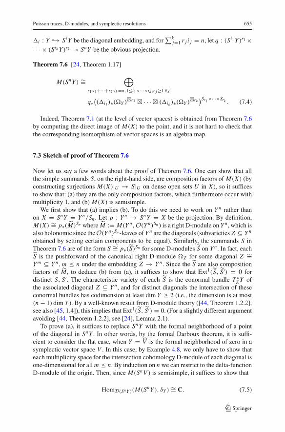
Theorem 7.6 [24, Theorem 1.17]
M(SnY ) ∼=⊕
r1·i1+···+rk ·ik=n,1≤i1<···<ik ,r j≥1∀ j
q∗(
(�i1)∗(�Y )�r1 � · · ·� (�ik )∗(�Y )�rk)Sr1×···×Srk . (7.4)
Indeed, Theorem 7.1 (at the level of vector spaces) is obtained from Theorem 7.6by computing the direct image of M(X) to the point, and it is not hard to check thatthe corresponding isomorphism of vector spaces is an algebra map.
7.3 Sketch of proof of Theorem 7.6
Now let us say a few words about the proof of Theorem 7.6. One can show that allthe simple summands S, on the right-hand side, are composition factors of M(X) (byconstructing surjections M(X)|U → S|U on dense open sets U in X ), so it sufficesto show that: (a) they are the only composition factors, which furthermore occur withmultiplicity 1, and (b) M(X) is semisimple.
We first show that (a) implies (b). To do this we need to work on Yn rather thanon X = SnY = Yn/Sn . Let p : Yn → SnY = X be the projection. By definition,M(X) ∼= p∗( ˜M)Sn where ˜M := M(Yn,O(Yn)Sn ) is a right D-module on Yn , which isalso holonomic since theO(Yn)Sn -leaves ofYn are the diagonals (subvarieties Z ⊆ Yn
obtained by setting certain components to be equal). Similarly, the summands S inTheorem 7.6 are of the form S ∼= p∗(˜S)Sn for some D-modules ˜S on Yn . In fact, each˜S is the pushforward of the canonical right D-module �Z for some diagonal Z ∼=Ym ⊆ Yn,m ≤ n under the embedding Z → Yn . Since the ˜S are also compositionfactors of ˜M , to deduce (b) from (a), it suffices to show that Ext1(˜S, ˜S′) = 0 fordistinct S, S′. The characteristic variety of each ˜S is the conormal bundle T ∗Z Y ofthe associated diagonal Z ⊆ Yn , and for distinct diagonals the intersection of theseconormal bundles has codimension at least dim Y ≥ 2 (i.e., the dimension is at most(n − 1) dim Y ). By a well-known result from D-module theory ([44, Theorem 1.2.2],see also [45, 1.4]), this implies that Ext1(˜S, ˜S′) = 0. (For a slightly different argumentavoiding [44, Theorem 1.2.2], see [24], Lemma 2.1).
To prove (a), it suffices to replace SnY with the formal neighborhood of a pointof the diagonal in SnY . In other words, by the formal Darboux theorem, it is suffi-cient to consider the flat case, when Y = V is the formal neighborhood of zero in asymplectic vector space V . In this case, by Example 4.8, we only have to show thateach multiplicity space for the intersection cohomology D-module of each diagonal isone-dimensional for allm ≤ n. By induction on n we can restrict to the delta-functionD-module of the origin. Then, since M(SnV ) is semisimple, it suffices to show that
HomD(SnY )(M(SnY ), δY ) ∼= C. (7.5)
123

656 P. Etingof, T. Schedler
Finally, (7.5) can be restated without using D-modules in the form of the followinglemma, which plays a central role in the proof, and concludes our sketch of it:
Lemma 7.7 [24, Lemma 2.3] The space of symmetric polydifferential operators ψ :O(V )⊗(n−1) → O(V ) invariant under Hamiltonian flow is one dimensional, andspanned by the multiplication map. The same holds for polydifferential operators onthe completion O(V ) = O(V ) of O(V ) with respect to the augmentation ideal.
Proof It suffices to pass to the formal completion and consider polydifferential oper-ators on O(V ). Such polydifferential operators are determined by their value onelements f ⊗(n−1) for f ∈ O(V ), since they are symmetric and hence determinedby their restriction to Symn−1O(V ). Furthermore, we can assume that f ′(0) �= 0,since the complement of this locus in the pro-vector space O(V ) has codimensionequal to dim V ≥ 2.
Write V ∼= C2n with the standard symplectic form ω =∑dim Vi=1 dxi ∧ dyi . Apply-
ing the formal Darboux theorem, there is a formal symplectomorphism of V whosepullback takes f to x1 (i.e., f can be completed to a coordinate system in whichthe symplectic form is the standard one), so we can assume f = x1. Since all for-mal symplectic automorphisms are obtained by integrating Hamiltonian vector fields,it suffices to consider the value ψ(x⊗(n−1)
1 ). This value must be a function that, incoordinates, depends only on x1, since such functions are the only ones which areinvariant under all symplectic automorphisms fixing x1. By linearity and invarianceunder conjugation by rescaling x1 (and applying the inverse scaling to y1), we deducethat ψ(x⊗(n−1)
1 ) = λ · xn−11 for some λ ∈ C. Thus, on x⊗(n−1)1 , ψ coincides with λ
times the multiplication operator, f1⊗· · ·⊗ fn−1 �→ λ f1 · · · fn−1. The latter operatoris evidently symmetric and invariant under Hamiltonian flow. On the other hand, wehave argued that a symmetric operator invariant under Hamiltonian flow is uniquelydetermined by its value on x⊗(n−1)
1 . Soψ is equal toλ times themultiplication operator,as desired. ��
As a by-product, we obtain the following theorem:
Theorem 7.8 [24, Theorem 1.6] Let V be a finite-dimensional symplectic vec-tor space, and realize V n−1 as the set of elements (v1 . . . , vn) ∈ V n such that∑n
i=1 vi = 0. Then, HP0(O(V n−1/Sn))∗ ∼= C spanned by the augmentation mapO(V n−1)→ C. In other words, the Lie algebra g of Sn-invariant Hamiltonian vectorfields on V n−1 is perfect: g = [g, g].
8 Structure of M(X) for complete intersections with isolatedsingularities
In this section we discuss results from [25, Sect. 5] and [23] concerning M(X) andHPDR∗ (X) when X is a complete intersection surface with isolated singularities (ormore generally of arbitrary dimension, if one suitably defines the Lie algebra g ofHamiltonian vector fields). In particular, wewill recover topological information aboutthe singularities, including the Milnor numbers and genera, and find examples where
123

Poisson traces, D-modules, and symplectic resolutions 657
M(X) is not semisimple. For concreteness, we will take X to be a surface in C3
throughout most of the section and explain at the end how the arguments extend togeneral (locally) complete intersections (of arbitrary dimension) in complex affinespace.
8.1 Main results for surfaces in C3
Let X = { f = 0} ⊆ C3 = SpecC[x1, x2, x3] be a surface with f irreducible. It isnaturally Poisson, with bracket {x1, x2} = fx3 together with cyclic permutations ofthe indices. We will be interested particularly in f having two nice properties:
Definition 8.1 A variety X is said to have isolated singularities if the singular locusof X is finite. A function f ∈ C[x1, . . . , xn] is said to have isolated singularities if{ f = 0} is a variety with isolated singularities.
Definition 8.2 A function f ∈ C[x1, . . . , xn] is quasi-homogeneous of weight | f | =m ≥ 1 with respect to weights |xi | = ai ≥ 1 if f is a linear combination of monomialsof degree m with respect to these weights.
Note that f is quasi-homogeneous if and only if X = { f = 0} is conical withrespect to theC× action λ · (x1, . . . , xn) = (λa1x1, . . . , λan xn), i.e., this action (whichcontracts to the origin) preserves X . Note that if f is quasi-homogeneous with isolatedsingularities, then since the singular locus is preserved under the action ofC×, it mustbe identically {0} (or empty).
Example 8.3 In the case that f ∈ C[x1, x2, x3] is quasi-homogeneous with weight mwith respect to |xi | = ai , we see that the Poisson bracket has degree d := m − (a1 +a2+a3). If moreover f has isolated singularities (i.e., its singular locus is {0}), then Xis well known to be isomorphic to a duVal singularity,C2/� for� < SL(2,C) a finitesubgroup, if d < 0; to have a simple elliptic singularity at the origin if d = 0; and tohave neither a du Val nor elliptic singularity if d > 0. In particular, up to isomorphism,in the case d < 0 (a du Val singularity) X is isomorphic to one of the following (see,e.g., [10] and [17, Proposition 2.3.2]):
Am−1: � = Z/m, a1 = 2, a2 = a3 = m, f = xm1 + x22 + x23 , (8.1)
Dm+2: � = D2m, a1 = 2, a2 = m, a3 = m + 1, f = xm+11 + x1x22 + x23 ,
(8.2)
E6: � = ˜A4, a1 = 3, a2 = 4, a3 = 6, f = x41 + x32 + x23 , (8.3)
E7: � = ˜S4, a1 = 4, a2 = 6, a3 = 9, f = x31 x2 + x32 + x23 , (8.4)
E8: � = ˜A5, a1 = 6, a2 = 10, a3 = 15, f = x51 + x32 + x23 ; (8.5)
and in the case d = 0 (elliptic), then X is isomorphic to one of the following forms:
˜E6: a1 = a2 = a3 = 1, f = x31 + x32 + x33 + λx1x2x3, (8.6)˜E7: a1 = a2 = 1, a3 = 2, f = x41 + x42 + x23 + λx1x2x3, (8.7)
123

658 P. Etingof, T. Schedler
˜E8: a1 = 1, a2 = 2, a3 = 3, f = x61 + x32 + x23 + λx1x2x3. (8.8)
Notation 8.4 For a possibly singular complex algebraic or analytic variety X , letH∗top(X) denote the topological cohomology of X .
Notation 8.5 For s ∈ X an isolated singularity, let μs denote the Milnor numberat s. Let gs denote the “reduced genus” of the singularity at s, which we define asgs = dim Hdim X−1(Y,OY ), for ρ : ˜X → X any resolution of singularities andY = ρ−1(s) (this definition does not depend on the choice of resolution).
By [33,48], if Xt is a smoothing of X , then for B(s) a small ball about s, Xt ∩ B(s)is homotopic to a bouquet of μs spheres of dimension dim X . In the case X is ahypersurface in Cn , the Milnor number can be described as the codimension inO(X)
of the ideal generated by the partial derivatives of f .
Theorem 8.6 [23, Theorem 2.4] If X is a surface in C3 with isolated singularitiess1, . . . , sk , then HPDR∗ (X) ∼= H2−∗
top (X)⊕⊕ki=1 C
μsi , placing Cμsi in degree zero.
Theorem 8.6 follows from the following structure theorem for M(X) in this case.Let Z ⊆ X be the singular locus and j : X\Z → X the open embedding. Recallthat, for M a holonomic right D-module on X\Z , there are pushforward complexesof D-modules j!M, j∗M on X and a holonomic D-module j!∗M on X satisfying theadjunction properties Hom(H0 j!M, N ) = Hom(M, j !N ) and Hom(N , H0 j∗M) =Hom( j !N , M) (for j !N = j∗N the restriction of N to the open subset U ); alsoj!∗M is the minimal extension, which means for example that j!∗M is simple if andonly if M is. Since X\Z is a smooth symplectic variety, j !M(X) = �X\Z , whichimplies that M(X) has a composition series one of whose composition factors is theintersection cohomology D-module of X , IC(X) = j!∗�X\Z , and the others which areD-modules supported on the singular locus, and hence are delta-function D-modulessince the singular locus is finite. Let M(X)ind be the indecomposable summand ofM(X) which has IC(X) as a composition factor.
Theorem 8.7 [23, Theorem 2.7] Let X = { f = 0} ⊆ C3 have singular locus Z ={s1, . . . , sk} (with the si distinct). Then there is a short exact sequence
0→ H0 j!�X\Z → M(X)→k
⊕
i=1δμsi → 0.
Conjecture 8.8 [23, Conjecture 3.8]1 Under the same hypotheses as in Theorem 8.7,we have a short exact sequence
0→ H0 j!�X\Z → M(X)ind→⊕
i
δgsi → 0.
1 For a proof that the conjecture above is the same as the statement from [23], see Proposition 3.13 of thearXiv version 1401.5042 of [23], and apply Grothendieck–Serre duality to identify Hdim Y (Y,OY ) withglobal sections of the logarithmic canonical bundle on Y . See also the second paragraph of the proof of [14,Lemma 2.5].
123

Poisson traces, D-modules, and symplectic resolutions 659
Theorem 8.9 [23, Proposition 3.11]Conjecture 8.8 is true if f is quasi-homogeneous.
Remark 8.10 Theorem 8.7 shows that there are delta-function submodules of M(X)
which are not direct summands whenever H0 j!�X\Z � IC(X), the minimal extensionof �X\Z . Equivalently, this holds whenever Ext1(IC(X), δs) �= 0 for some points ∈ Z . Since Ext1(IC(X), δs) ∼= Ext1(δs, IC(X))∗ by Verdier duality, we actuallysee that M(X) is not semisimple whenever possible, i.e., whenever there exists anonsemisimple extension of �X\Z to X . One can compute that Ext1(IC(X), δs) ∼=H1top(Us\{s})whereUs is some contractible neighborhood of s (see [14, Lemma 3.5],
similar to [20, Lemma 4.3]), which exists by [27], cf. also [48, 2.10]. Here Us\{s}is homotopic to the topological link of s. Thus, we see that M(X) is not semisimplewhenever the link has nonzero first Betti number.
Remark 8.11 Taking the special case where X is a cone over a smooth curve � in P2
of degree d, recall that the reduced genus of the singularity is g = (d−1)(d−2)2 (the
same as the genus of �) and the Milnor number is μ = (d − 1)3. In this case, wesee that H1
top(X\{0}) ∼= H1top(�) (since X\{0} is homotopic to a nontrivial S1-bundle
over �). Therefore, by Remark 8.10 we obtain that H0 j!�X\{0} is an extension givenby a short exact sequence of the form
0→ δ2g0 → H0 j!�X\{0} → IC(X)→ 0. (8.9)
We obtain from Theorem 8.9 that M(X)ind has a filtration with subquotientsδ2g, IC(X), and δg , in that order. In particular, for g > 0, it is not semisimple, andmoreover not self-dual (there is twice the multiplicity of δ function D-modules on thebottom as on the top). From Theorem 8.7 we see that M(X) ∼= M(X)ind ⊕ δ
μ−g0 .
8.2 The family M(Xt) of fiberwise D-modules on a smoothing
The results can be reinterpreted in terms of a smoothing. Namely, we can consider allthe level sets Xt := { f = t} ⊆ C3 of f inC3 as t ∈ C varies, which for generic t willbe smooth. It is then well known that, for generic t , dim H2
top(Xt ) = dim H2top(X)+
∑
s∈Z μs , where again Z ⊆ X is the singular locus which we assume is finite; thisis a consequence of the fact from [33,48] that, for every s ∈ Z and 0 < |t | � 1,the intersection of Xt with a small ball about s ∈ C3 is homotopic to a bouquet ofμs 2-spheres. As a result, Theorem 8.6 implies that dimHP0(O(X)) = dim H2
top(Xt )
for generic t . Since Xt is a smooth symplectic surface, H2top(Xt ) ∼= HP0(O(Xt )) (by
Example 5.2). Thus, near t = 0 the family HP0(Xt ) of vector spaces has constantdimension, i.e., forms a vector bundle. We have proved:
Corollary 8.12 [23, Corollary 1.4] Assume X = { f = 0} ⊆ C3 has isolated sin-gularities. Then, the sheaf HP0(O(Xt )) on C is a vector bundle near t = 0 of rankdim H2
top(X)+∑
s∈Z μs = dimHP0(O(X)). The generic fiber is H2top(Xt ).
The entire Poisson-de Rham homology similarly forms a graded vector bundle [23,Corollary 2.5], since the dimension of Hi
top(Xt ) does not depend on t for i ∈ {0, 1},and this equals the dimension of HPDR
2−i (X).
123
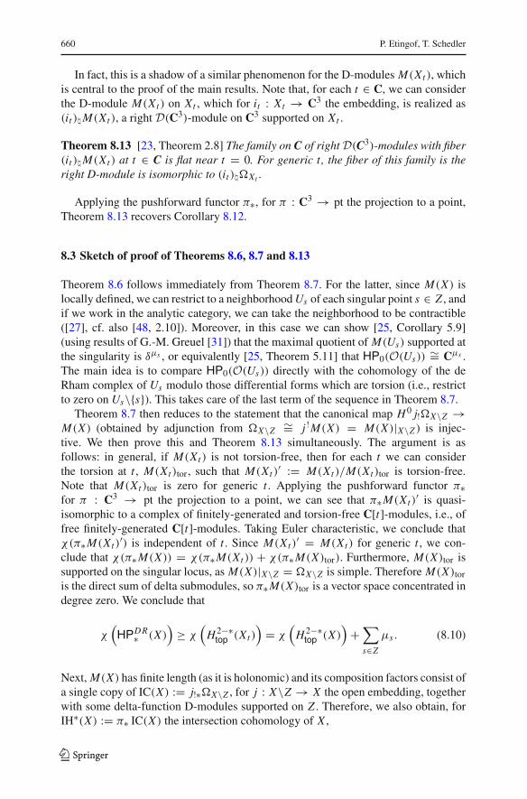
660 P. Etingof, T. Schedler
In fact, this is a shadow of a similar phenomenon for the D-modules M(Xt ), whichis central to the proof of the main results. Note that, for each t ∈ C, we can considerthe D-module M(Xt ) on Xt , which for it : Xt → C3 the embedding, is realized as(it )�M(Xt ), a right D(C3)-module on C3 supported on Xt .
Theorem 8.13 [23, Theorem 2.8] The family on C of rightD(C3)-modules with fiber(it )�M(Xt ) at t ∈ C is flat near t = 0. For generic t , the fiber of this family is theright D-module is isomorphic to (it )��Xt .
Applying the pushforward functor π∗, for π : C3 → pt the projection to a point,Theorem 8.13 recovers Corollary 8.12.
8.3 Sketch of proof of Theorems 8.6, 8.7 and 8.13
Theorem 8.6 follows immediately from Theorem 8.7. For the latter, since M(X) islocally defined, we can restrict to a neighborhoodUs of each singular point s ∈ Z , andif we work in the analytic category, we can take the neighborhood to be contractible([27], cf. also [48, 2.10]). Moreover, in this case we can show [25, Corollary 5.9](using results of G.-M. Greuel [31]) that the maximal quotient of M(Us) supported atthe singularity is δμs , or equivalently [25, Theorem 5.11] that HP0(O(Us)) ∼= Cμs .The main idea is to compare HP0(O(Us)) directly with the cohomology of the deRham complex of Us modulo those differential forms which are torsion (i.e., restrictto zero on Us\{s}). This takes care of the last term of the sequence in Theorem 8.7.
Theorem 8.7 then reduces to the statement that the canonical map H0 j!�X\Z →M(X) (obtained by adjunction from �X\Z ∼= j !M(X) = M(X)|X\Z ) is injec-tive. We then prove this and Theorem 8.13 simultaneously. The argument is asfollows: in general, if M(Xt ) is not torsion-free, then for each t we can considerthe torsion at t , M(Xt )tor, such that M(Xt )
′ := M(Xt )/M(Xt )tor is torsion-free.Note that M(Xt )tor is zero for generic t . Applying the pushforward functor π∗for π : C3 → pt the projection to a point, we can see that π∗M(Xt )
′ is quasi-isomorphic to a complex of finitely-generated and torsion-free C[t]-modules, i.e., offree finitely-generated C[t]-modules. Taking Euler characteristic, we conclude thatχ(π∗M(Xt )
′) is independent of t . Since M(Xt )′ = M(Xt ) for generic t , we con-
clude that χ(π∗M(X)) = χ(π∗M(Xt )) + χ(π∗M(X)tor). Furthermore, M(X)tor issupported on the singular locus, as M(X)|X\Z = �X\Z is simple. Therefore M(X)toris the direct sum of delta submodules, so π∗M(X)tor is a vector space concentrated indegree zero. We conclude that
χ(
HPDR∗ (X))
≥ χ(
H2−∗top (Xt )
)
= χ(
H2−∗top (X)
)
+∑
s∈Zμs . (8.10)
Next, M(X) has finite length (as it is holonomic) and its composition factors consist ofa single copy of IC(X) := j!∗�X\Z , for j : X\Z → X the open embedding, togetherwith some delta-function D-modules supported on Z . Therefore, we also obtain, forIH∗(X) := π∗ IC(X) the intersection cohomology of X ,
123

Poisson traces, D-modules, and symplectic resolutions 661
χ(
HPDR∗ (X))
= χ(IH∗(X))+ m, (8.11)
wherem is the number of delta-function D-modules appearing as composition factorsof M(X). Putting (8.10) and (8.11) together, we get
χ(IH∗(X))+ m ≥ χ(
H2−∗top (X)
)
+∑
s∈Zμs . (8.12)
Now we restrict again to X = Us , a contractible neighborhood of s. As we saw above,in this case μs is the length of the maximal quotient of M(Us) supported at s. Let Kbe the maximal submodule of M(X)ind supported at s. Let m′ be the length of K (soK ∼= δm
′s ). Then, we have an exact sequence 0→ K → M(X)|Us → δμs → 0, and
hence m = μs + m′. Since Us is contractible, we obtain from all of this:
χ(IH∗(Us))+ m′ ≥ 1. (8.13)
Finally we explicitly compute χ(IH∗(Us)) [25, Proposition 5.9] using the classi-cal formula [28, Sect. 6.1], obtaining χ(IH∗(Us)) = 1 − dim H1
top(Us\{s}). We
conclude m′ ≥ dim H1top(Us\{s}). On the other hand, we compute in general that
dim H1top(Us\{s}) = dim Ext1(IC(Us), δs), the maximum possible size of a submod-
ule of M(X) supported at s which does not contain a direct summand of M(X). Inother words, this is one less than the length of H0 j!�X\Z itself. Therefore, the mapH0 j!�X\Z → M(X) is injective, and moreover, (8.13) is an equality. The formerfinishes the proof of Theorem 8.7, and the latter proves Theorem 8.13.
8.4 Sketch of proof of Theorem 8.9
Here, following [23, Sect. 6], we sketch the proof of Theorem 8.9 under the additionalassumption that f is actually homogeneous, i.e., ai = |xi | = 1 for all i . The generalcase does not significantly change the details, and thismakes things a bit more concreteand easier to follow.
Let Eu =∑
i xi∂i be the Euler vector field. Themain idea is that there is a canonicalendomorphism TEu ∈ EndD(C3)(i�M(X)) which descends from the endomorphism
� �→ Eu ·� of left multiplication on D(C3). (Actually, M(X) is weakly equivariant,which means that i�M(X) is a graded right D(C3)-module, such that for homoge-neous � ∈ i�M(X), |�|� = TEu(�) − � · Eu; see Sect. 9.) Let TEu also denote thecorresponding endomorphism of M(X). Then, M(X) decomposes as a direct sum ofthe generalized eigenspaces of TEu; call them M(X)m .
Next, the degree inwhichM(X)ind appears is the degree d of the Poisson bivector σ ,since the action of Eu by right multiplication on the symplectic volume form of X\{0}is multiplication by d, and the symplectic volume form is the image of the generator1 under the canonical quotient DX\{0} � �X\{0} (as it is invariant under Hamiltonianflow). So M(X)d is a direct sum of M(X)ind and some δ-function D-modules. By
123

662 P. Etingof, T. Schedler
Theorem 8.7, we have an exact sequence
0→ H0 j!�X\{0} → M(X)d → δ0 ⊗ HP0(O(X))d → 0. (8.14)
Since the Poisson bracket has degree d and the only elements of weight zero areconstants which are central, {O(X),O(X)} is spanned by elements of weight > d,and hence HP0(O(X))d = O(X)d . In [23, Proposition 3.11] this space is shown tohave dimension g0 (using the identification of Hdim X−1(D,OD)with the vector spaceappearing in [23, Conjecture 3.8] as we remarked in the footnote to Conjecture 8.8).Therefore, Theorem 8.9 reduces to the statement thatM(X)d itself is indecomposable,hence M(X)d = M(X)ind.
To show this, we first claim that for each m ∈ Z, TEu is actually central inEnd(M(X)m). Indeed, every endomorphism of M(X) descends from left multipli-cation T� : � �→ � ·� by some � ∈ D(C3). Since [TEu, T� ] = T[Eu,�] and [Eu,−]is a semisimple operator on D(C3), it follows that [TEu,−] is a semisimple opera-tor on End(M(X)). On each generalized eigenspace M(X)m we therefore have that[TEu,End(M(X)m)] = 0.
As a result, TEu preserves every direct summand of M(X)m for every m. For acontradiction, suppose that there is a direct summand K of M(X)d supported at theorigin. We can assume K ∼= δ0. Now T ′ := TEu − d Id is a nilpotent endomorphismof M(X)d which preserves K , hence T ′|K = 0.
To obtain a contradiction, let v : M(X)d → K ∼= δ0 be the projection. Let N bethe space of smooth distributions onC3 and w : δ0 → N the inclusion. The main stepin the proof is the following (which is a slightly weaker version of [23, Lemma 6.1]):
Lemma 8.14 There is a Hamiltonian-invariant distribution φv ∈ N such that φv ·(Eu−d) = w(v(1)).
Equivalently, there is a solution ϕ ∈ Hom(M(X)d , N ), with ϕ(1) = φv , such thatϕ ◦ T ′ = w ◦ v. Since w ◦ v|K �= 0, it follows that T ′|K �= 0, which is a contradiction.
To prove Lemma 8.14, we construct φv explicitly. By (8.14) we can associate withv an element of HP0(O(X))∗d . Let Q ∈ HP0(O(X))d be the dual of v under theHermitian pairing on HP0(O(X))d :
〈P, Q〉 :=∫
S5∩XPQω ∧ ω/dr,
where ω is the rational volume form on X (the inverse of the Poisson bivector), and ris the radial coordinate function. Then, we partially define φv by:
φv(α) = − 2∫
Xαω ∧ Qω.
This converges when α vanishes to order greater than d [23, Lemma 6.2], and we canextend it arbitrarily to a linear functional on all ofC∞c (C3). The result is annihilated byall Hamiltonian vector fields which vanish to order greater than d, but since the weightof σ is d, this includes all Hamiltonian vector fields. Thus φv ∈ Hom(M(X)d , N ).
123

Poisson traces, D-modules, and symplectic resolutions 663
We claim that φv · (Eu−d) = w(v(1)), which completes the proof. By defini-tion of Q ∈ HP0(O(X))d = O(X)d , the RHS has the property w(v(1))(PH) =〈Q, P〉H(0) for all P ∈ O(X)d and H ∈ C∞c (Cn). We have to show the same forthe LHS. It suffices to show this for a single choice of H , and the identity thereforereduces to an explicit computation: choosing H(x) = h(|x |2) for h a smooth realfunction with h(0) �= 0, we obtain
(φv · (Eu−d))(PH) = − 2∫
XPQ Eu(H)ω ∧ ω
= − 2∫ ∞
0dr · r · h′(r2) · 〈P, Q〉
= 〈P, Q〉h(0) = 〈P, Q〉H(0).
The first equality uses that we can choose the extension of φv from functions vanishingto order > d at 0 to all functions in such a way that we project away from a space offunctions supported in an arbitrarily small neighborhood of zero (and that φv ·(Eu−d)
does not depend on the choice of extension). This completes the sketch.
8.5 Generalization to locally complete intersections and higher dimension
Finally, we explain how to generalize from surfaces in C3 to general locally completeintersections of arbitrary dimension.
Suppose that X is a complete intersection surface in Cn , i.e., X = { f1 = · · · =fn−2 = 0}. Then, X has a Poisson structure, called the Jacobian Poisson structure,given by the skew-symmetric biderivation σ = i∂1∧···∧∂n (d f1 ∧ · · · ∧ d fn−2)|X , i.e.,σ = ∑
i< j σi, j (∂i ∧ ∂ j )|X for σi, j = (−1)i+ j−1 ∂( f1,..., fn−2)∂(x1,...,xi ,...,x j ,...,xn)
the Jacobiandeterminant (omitting xi and x j from the denominator). Explicitly,
{g, h} = ∂( f1, . . . , fn−2, g, h)
∂(x1, . . . , xn).
With thismodification all of the preceding results generalizewithout change, exceptthat now the family Xt should be defined by picking a generic lineC·(c1, . . . , cn−2) ⊆Cn−2, and setting Xt = { fi = ci }ni=1 ⊆ Cn , which will be smooth for generic t . Thequasi-homogeneous condition is replaced by the condition that all of the fi be quasi-homogeneous with respect to fixed weights ai = |xi | (but the degrees of the fi can bedifferent).
Next, we explain how to generalize to varieties of higher dimension. If X = { f1 =· · · = fn−k = 0} ⊆ Cn is a complete intersection of dimension k ≥ 2, then X isequipped with a canonical skew-symmetric multiderivation �X : O(X)⊗ dim X →O(X),
�X := i∂1∧···∧∂n (d f1 ∧ · · · ∧ d fn−k)|X .
123

664 P. Etingof, T. Schedler
Given a (k−2)-form α ∈ �k−2(X), we can associate a vector field, ξα := i�X (dα),which we call the Hamiltonian vector field of α. Let g be the set of all Hamiltonianvector fields on X . We can check that g is a Lie algebra, using the formula [ξα, ξβ ] =ξLξα β [25, Sect. 3.4], which one can check in local coordinates.
Remark 8.15 The vector fields ξα actually make sense as vector fields on all of Cn :since α := d f1 ∧ · · · ∧ d fn−k ∧ α is a well-defined (n − 1)-form on Cn , we obtain˜ξα := i∂1∧···∧∂n (d f1 ∧ · · · ∧ d fn−k ∧ α), a well-defined vector field on Cn , which isHamiltonian on each level set Xc1,...,cn−k = { fi = ci }n−ki=1 . Thus, the Lie algebra ofHamiltonian vector fields on each Xc1,...,cn−k is the same Lie algebra g.
Thus, we can replaceHP0(O(X)) by (O(X))g = HPg−DR0 (X) and similarly for Xt
(where now we define Xt using a generic line C · (c1, . . . , cn−k) ⊆ Cn−k). Similarlywe can replaceM(X) andM(Xt ) byM(X, g) andM(Xt , g). (In view of Remark 8.15,we have the explicit description (it )�M(Xt , g) = (gDCn + IXtDCn )\DCn .) With thischange, all of the results and proofs continue to go through in the same manner.
Finally, since the D-module M(X) is defined locally, we actually do not needto require that X globally be a complete intersection, only that it locally admitsthis structure, provided that there is a global skew-symmetric multiderivation �X :O⊗ dim X
X → OX which is nonvanishing on the smooth locus. We do not require Xto be affine. The notion of isolated singularities still makes sense. We can replace thequasi-homogeneous condition by the condition that, at every point x ∈ X , the formalneighborhood Xx of the point is isomorphic to a complete intersection in C
n0 defined
by quasi-homogeneous functions (with respect fixed weights that can depend on thepoint x chosen), i.e., that X be formally locally conical.
8.6 Relationship to the Bernstein–Sato polynomial
In [14], following a suggestion of the first author, the second author and T. Bitounrelate these results to the theory of the Bernstein–Sato polynomial. Namely, the latterinvolves the study, for f ∈ C[x1, . . . , xn] = O(Cn) and λ ∈ C, of the left D(Cn)-module D(Cn) · f λ. Let us recall the definition. Let U := Cn\{ f = 0}, so thatD(U ) = D(Cn)[ f −1] and O(U ) = O(Cn)[ f −1]. Let D(U ) · f λ be the D(U )-module which as a O(U )-module is the trivial line bundle on U together with anonvanishing section denoted f λ, and the D(U ) action is defined by the formulaξ · f λ = λξ( f ) f −1 · f λ for every derivation ξ ∈ Vect(U ). In other words,D(U )· f λ =D(Cn)[ f −1]/D(Cn)[ f −1] · (∂i − λ f −1 fxi | 1 ≤ i ≤ n) with generator denoted byf λ. Let D(Cn) · f λ be the D(Cn)-submodule of D(U ) · f λ generated by f λ. Wesimilarly define the D(Cn)[s]-module D(Cn)[s] · f s . For every right D(Cn) module,let M� := M ⊗O(Cn) �−1Cn be the associated left D(Cn)-module. For X = { f = 0},one has the following canonical surjection of left D(Cn)-modules:
i�M(X, g)� = i�M(X, g)⊗O(Cn) �−1Cn � D(Cn) f λ/D(Cn) f λ+1,1⊗ (∂1 ∧ · · · ∧ ∂n) �→ f λ, (8.15)
123

Poisson traces, D-modules, and symplectic resolutions 665
as well as a canonical map
i�M(X, g)�→ D(Cn)[s] f s/D(Cn)[s] f s+1, (8.16)
which is surjective for f quasi-homogeneous. (Since then for Eu the Euler vectorfield, we have | f |−1 Eu · f s = s f s .) Using the maps (8.15) and (8.16), we prove thefollowing. Let Z ⊆ X continue to be the singular locus, which we assume to be finite.For each s ∈ Z , let Us be a contractible neighborhood of s. Define
K := ker(H0 j!�X\Z � j!∗�X\Z ) ∼=⊕
s∈ZExt1( j!∗�X\Z , δs)
∗ ⊗ δs
∼=⊕
s∈ZHn−2top (Us\{s})∗ ⊗ δs
(for the last isomorphism see [14, Lemma 3.5], cf. Example 8.10). Then:
Theorem 8.16 [14] Suppose that n ≥ 3 and { f = 0} has isolated singularities.Then, (8.15) produces an isomorphism (i�M(X, g)ind/K )� ∼= D(Cn) f −1/O(Cn). Ifmoreover f is quasi-homogeneous, (8.16) produces an isomorphism i�M(X, g)� ∼=D(Cn)[s] f s/D(Cn)[s] f s+1.Corollary 8.17 Conjecture 8.8 is equivalent to the statement: if { f = 0} is irre-ducible with isolated singularities, then the length of the left D(Cn)-module D(Cn) ·f −1/O(Cn) is one more than the sum of the reduced genera of the singularities.
This formula was motivated by a similar phenomenon discovered by T. Bitounin characteristic p > 0: Let f be a polynomial with rational coefficients in n ≥ 3variableswhich is absolutely irreducible, i.e., it remains irreducible overC, and assumethat { f = 0} has a unique singular point. For a field F let An
F be the affine space overthe field F and D(An
F ) be the ring of Grothendieck differential operators on AnF .
Then, for p sufficiently large, we can consider the local cohomologyD(AnFp
)-module
O(AnFp
)[ f −1]/O(AnFp
),which turns out to be generated by f −1 (hence fully analogoustoD(Cn) · f −1/O(Cn) in characteristic zero). In [9], it is proved that, for sufficientlylarge p the length of this D(An
Fp)-module is one more than the “p-genus” of the
singularity, which is defined as the dimension of the “stable part” of Hn−2(Yp,OYp ),for Yp the exceptional fiber of a resolution of singularities of X p := { f = 0} ⊆ AFp
,where the stable part refers to the intersection of the images of all powers of theFrobenius morphism. See [9,14] for details.
The above results also have a direct application to the Bernstein–Sato polynomial.Recall that the Bernstein–Sato polynomial is defined as the annihilator in C[s] ofD(Cn)[s] f s/D(Cn)[s] f s+1. Using the surjections D(Cn)[s] f s � D(Cn) · f λ, itfollows that, if D(Cn) · f λ �= D(Cn) · f λ+1, then λ is a root of this polynomial. Theconverse question is interesting and little is known aside from [43, Proposition 6.2],which says that the converse holds if additionally λ−m is not a root for any positiveinteger m. The results above imply a converse in the quasi-homogeneous case:
123

666 P. Etingof, T. Schedler
Corollary 8.18 [14,52] For f quasi-homogeneous with an isolated singularity andλ ∈ C, ifλ is a root of the Bernstein–Sato polynomial, thenD(Cn)· f λ �= D(Cn)· f λ+1.
M. Saito has also demonstrated in [52, Example 4.2] a counterexample to thisassertion when the quasi-homogeneity assumption is removed.
9 Weights on homology of cones
We continue to work over k = C. In Sect. 8.4, we used that if O(X) is graded (i.e.,X admits a C×-action) and Poisson with a homogeneous Poisson bracket (which wasthe case there for X a quasi-homogeneous surface in C3), then HP0(O(X)) is alsononnegatively graded. In this section we explain how in fact HPDR∗ (X) is bigraded,and consider its bigraded Hilbert–Poincaré polynomial (i.e., a Laurent polynomial intwo variables). We give several examples (without proofs) that demonstrate that onerecovers in this way many special polynomials from combinatorics.
9.1 Weakly equivariant D-modules and bigrading on Poisson-de rhamhomology
As noted in Sect. 8.4 in a particular situation, when O(X) is graded, then M(X) isweakly C×-equivariant. Let us first recall the general definition:
Definition 9.1 LetO(X) be graded and i : X → V aC×-equivariant embedding intoa smooth variety V , i.e., O(V ) is graded and IX is a graded ideal. Then, a weaklyC×-equivariant D-moduleM on X is one associated with a graded rightD(V )-modulei�M on V supported on i(X).
Call this grading on i�M(X) the weight grading. In this case, the pushforwardπ∗M(X) = i�M(X) ⊗L
D(V )O(V ) under the map π : X → pt is a complex of
weight graded vector spaces, since O(V ) is also a graded D(V )-module. Therefore,thePoisson-deRhamhomologyHPDR∗ (X) is bigraded. It is very interesting to computethis grading, which turns out to be closely related to important special polynomials.
Remark 9.2 The weight grading on M(X) comes from a decomposition of M(X)
itself. Let EuX and EuV be the Euler vector fields on X and V , i.e., EuX ( f ) = | f | fwhen f ∈ O(X) is homogeneous and similarly for V . Then, the endomorphism � �→EuV ·� of D(V ) induces an endomorphism of M(X), which can also be described as(i) the endomorphism induced by� �→ EuX � on the D-moduleDX on X , and (ii) theendomorphism of i�M which on homogeneous elements is� �→ |�|�−� ·EuV . Callthis endomorphism TEu. Then, M(X) decomposes into its generalized eigenspacesunder TEu, M(X) = ⊕
m∈Z M(X)m , and π∗M(X)m is concentrated in weight m.This decomposition is important to the proof of the following facts, as well as yieldinginteresting information in its own right. (It allows one to define, for instance, canonicalfiltrations on irreducible representations of the Weyl group: see Sect. 9.3 below.)
123

Poisson traces, D-modules, and symplectic resolutions 667
9.2 Symmetric powers of conical surfaces with isolated singularities
Let Y ⊆ C3 = Spec[x1, x2, x3] be a conical surface with singular locus {0}, i.e., Y ={ f = 0} where f is quasi-homogeneous with isolated singularities. In this context,⊕
n≥0 HP0(O(SnY ))∗ is again a graded algebra just as in Sect. 7.1, with grading givenby n, which we call the “symmetric power.” In fact, it is a bigraded algebra, with theadditional grading given by the weight on each summandHP0(O(SnY ))∗ (which willbe nonpositive, as it is dual to the nonnegative weight on O(SnY )). It turns out to bepossible to explicitly compute this bigraded vector space:
Theorem 9.3 [22, Theorem 1.1.14] There is a (noncanonical) isomorphism ofbigraded algebras,
Sym(HP0(O(Y ))∗[t]) ∼=⊕
n≥0HP0(O(SnY ))∗, (9.1)
assigning t bidegree (1,−| f |) (with 1 the symmetric power and−| f | the weight), andHP0(O(SnY ))∗ is assigned symmetric power n (on both sides of the equation).
Let JY := O(C3)/( fx1 , fx2 , fx3) be the Jacobi ring (so dim JY = μY is the Milnornumber of the singularity at the origin), and let its Hilbert–Poincaré polynomial beh(JY ; t) = ∑μY
i=1 tni . Note that for Y = C2/� with � < SL(2,C) finite, it iswell known that ni = di − 2 for di the degrees of the fundamental invariants ofthe Weyl group attached to � by the McKay correspondence (see (8.1)), i.e., C[h]Wis a polynomial algebra generated by elements of degrees di with h the reflectionrepresentation of W and |h∗| = 1.
Corollary 9.4 [22, (1.1.16)]∑
n≥0h(HP0(O(SnY ))∗; t)sn =
μY∏
i=1
∏
j≥0
1
1− tni+ jd s j+1.
In particular, the dimension of HP0(O(SnY )) is an(μY ) (7.3), the number of μY -multipartitions of n.
Remark 9.5 Weput “noncanonical” in parentheses because, unlike in the case of (7.1),we do not construct an explicit isomorphism. Note that the map of (7.1) still makessense here, but is no longer injective: indeed, if εn : O(SnY )→ C is the augmentationmap, then the map of (7.1) sends ε1tm−1 to εm for all m, but εm1 · · · εmk = εm1+···+mk
in the RHS, which shows that ε1&ε1 and ε1t both map to ε2. It does not appear thatthere exists a canonical isomorphism in general.
Now let us restrict to the special case where Y ∼= C2/� for � < SL(2,C) finite,i.e., Y is a du Val singularity. Then, SnY = C2n/(�n
� Sn) is a finite linear quotient ofa vector space, so the special case of (4.4) with V linear (i.e., [20, Proposition 4.16]),yields the entire structure of M(SnY ) for every n. We can therefore compute the entirePoisson-de Rham homology, with the help of [50, Theorem 5.1], which tells us in thiscase that a slight modification of (4.4) is an isomorphism of weakly C×-equivariantD-modules, applying on the right-hand side a shift in weight down by dim Z in eachsummand. The result is:
123

668 P. Etingof, T. Schedler
Corollary 9.6 For Y = C2/�, there is a (noncanonical) isomorphism of trigradedalgebras,
Sym(HP0(O(Y ))∗[t] ⊕ C[s] · u) ∼=⊕
n≥0HPDR∗ (O(SnY ))∗, (9.2)
where in the trigrading by symmetric power, weight, and homological degree, |t | =(1,−| f |, 0), |s| = (1, 0, 2), and |u| = (1,−2, 2). Thus on trigraded Hilbert serieswe obtain:
∑
n,m≥0h
(
HPDRm (O(SnY ))∗; t
)
snum =∏
j≥0
1
1−s j+1t−2u2 jμY∏
i=1
∏
j≥0
1
1−tni+ jd s j+1.
(9.3)In particular dimHPDR∗ (SnY ) = an(μY +1), the number of (μY +1)-multipartitionsof n (where μY also equals the number of irreducible representations of �).
9.3 The Nilpotent cone
Next let X ⊆ g be the cone of nilpotent elements in a semisimple Lie algebra g.Then, as explained in Example 6.6, HPDR∗ (X) ∼= Hdim X−∗(T ∗B), for T ∗B → Xthe Springer resolution. This is isomorphic to the cohomology of the flag varietyB itself. However, the source HPDR∗ (X) has an additional grading given from thedilation action on X . G. Lusztig proposed a formula for the graded Hilbert–Poincarépolynomial [50, Conjecture 8.1]. For W the Weyl group attached to g, and χ anirreducible representation of W , let Kg,χ (t) be the generalized Kostka polynomial,Kg,χ (t) := ∑
i≥0 t i dimHomW (χ, H2 dimB−2i (B)). Then, G. Lusztig’s suggestionwas:
h(
HPDR∗ (X); x, y)
=∑
χ∈Irrep(W )
Kg,χ (x2)Kg,χ (y−2). (9.4)
This is now a theorem [13, 1.1], again making use of [34].Note that the fact that H2 dimB−∗(B) has a W -action and that HPDR∗ (X) has a
second grading means that the isomorphism HPDR∗ (X) ∼= H2 dimB−∗(B) cannot becanonical (indeed, Kg,χ (y−2) would have to be a multiple of dim χ if there were abigrading compatible with the W action, and this is false in general). Instead, in [13],the authors construct a canonical family of filtrations on H2 dimB−∗(B), parameterizedby λ ∈ h∗reg, with h a Cartan subalgebra of g and h∗reg the complement of the coroothyperplanes.
Theorem 9.7 [13, Theorem 1.3] For every element λ ∈ h∗reg, there is a canonical
associated filtration Fλ on H2 dimB−∗(B) whose associated graded vector space isHPDR∗ (X). This is W-equivariant: Fw(λ) = w(Fλ).
Corollary 9.8 [13, Corollary 1.4] On every irreducible representation χ of W, toevery element λ ∈ h∗reg is associated a canonical filtration whose Hilbert series is
Kg,χ (y−2).
123

Poisson traces, D-modules, and symplectic resolutions 669
Example 9.9 [13, Example 1.5] Let g = sln and let χ = h∗ ⊗ sign ∼= Cn−1. Considerχ to be (in coordinates) Cn/C · (1, 1, . . . , 1), and make the same identification for h∗.Let λ ∈ h∗reg be the image of (a1, . . . , an) ∈ Cn . Then, the resulting filtration on χ
(the Vandermonde filtration) is: F2i−2 dimB(χ) is the span of (a j1 , . . . , a
jn ) for j ≤ i .
Finally, we can apply this to the classical W-algebras (see Example 6.7). This usesthe Springer correspondence, which associates with every irreducible representationχ of W a pair of a nilpotent coadjoint orbit Oχ ⊆ g∗ and a local system Lχ on Oχ .Identify g∗ ∼= g using the Killing form, so that Oχ ⊆ g, which allows us to considerirreducible representations χ such that Oχ = G · e.Corollary 9.10 [13, Corollary 2.5] The Hilbert–Poincaré polynomial ofHP0(O(S0e ))is
ydimG·e ∑
χ∈Irrep(W )|Oχ=G·edim Lχ · Kg,χ (y−2).
9.4 The hypertoric case
Let X be a hypertoric cone as inExample 6.9,which admits a symplectic resolution. LetA be the associated hyperplane arrangement (inCdim X/2) with |A| linear hyperplanes(whose normal vectors span Cdim X/2). Let �A(x, y, b) := �A(x, y, b1, . . . , bA) bethe polynomial defined by G. Denham in [16] using the combinatorial Laplacian.
Theorem 9.11 [50, Theorem 6.1] h(HPDR∗ (X); x, y) = y− dim X�A(x2 − 1, y−2 −1, y2).
The above formula is proved via the Tutte polynomial and symplectic leaves, whichare interesting in their own right. Let TA(x, y) denote the Tutte polynomial of thearrangement. The symplectic leaves of X are indexed by (coloop-free) flats F ⊆ A,cf. e.g., [51]. For each such we can define the restriction, AF , by intersecting withall the hyperplanes in F , and the localization, AF , by dividing by the intersection ofthese hyperplanes. Then, the above formula follows from the following one:
h(
HPDR∗ (X); x, y)
= y− dim X∑
F
TAF (x2, 0)TAF (0, y−2)y2|F |.
9.5 Conjectural description for conical symplectic resolutions
Finally, we sketch a conjectural description of the bigrading on HPDR∗ (X) in terms ofa deformation of resolution (which enhances Conjecture 6.1(b) for conical symplecticresolutions to incorporate the weights). Let ρ : ˜X → X be a projective conicalsymplectic resolution. Let ˜X → X be aC×-equivariant twistor deformation of ρ overC = SpecC[t] (see Remark 6.8). Note that the degree of t equals the degree of thesymplectic form on ˜X ; call this degree d.
123

670 P. Etingof, T. Schedler
Let˜θ : ˜X → C and θ : X → C be the projections to the base, and letXt := θ−1(t)and ˜Xt := ˜θ−1(t) be the fibers. By the argument of [56, Sect. 4.2], ˜θ is a topologicalfiber bundle (thanks to Y. Namikawa for pointing this out). Thus, the family of vectorspaces Hi ( ˜Xt ) is an algebraic vector bundle onC for each i equipped with the Gauss–Manin connection (corresponding to the right D-module Hi−dim X
˜θ∗� ˜X ). Using thisconnection we can uniquely trivialize the vector bundle (up to an overall scaling) andidentify it with Hi (˜X)⊗C[t]. (Note that the family of varieties ˜X is nontrivial, since˜Xt is affine for generic t but not for t = 0.)Let �i
cl be the space of holomorphic fiberwise closed differential forms on ˜X , i.e.,cycles in the complex of holomorphic differential forms modulo dt , for t the function˜X → C above. There is a natural map
� : �icl→ Hi (˜X)⊗ C[t]. (9.5)
Let Ki := coker(�). Then, Ki is finite dimensional and concentrated at t = 0.Thus, as a C[t]-module, Ki is a direct sum of Jordan blocks C[t]/tφ(i, j), forj = 1, 2, . . . , dim(Hi (˜X)) and φ(i, j) ∈ Z≥0 (where some of the Jordan blocksare allowed to be zero, in which case we set φ(i, j) = 0). Recall that d is the degreeof the generic symplectic form on X , which equals the degree of t .
Conjecture 9.12 h(HPDR∗ (X); x, y) = y−d·dim X/2 ∑
i, j xi yd·φ(dim X−i, j).
The cohomological degree zero case, i.e., h(HPDR0 (X); y) = y−d·dim X/2
∑
j yd·φ(dim X, j), should follow from Conjecture 6.1(a) using the direct interpreta-
tion of HPDR0 (X) ∼= HP0(O(X)) via functions on X . The difficulty appears to be in
relating HPDRi (X) for i > 0 to fiberwise closed differential forms on the family.
Remark 9.13 Note that the conjecture predicts in particular that HPDR∗ (X) lies onlyin weights which are multiples of d. This is not true in general if X does not admita symplectic resolution, even if it is a symplectic singularity (and hence has finitelymany leaves): in [18, Appendix A], many examples are constructed of X = V/Gwith V a symplectic vector space and G < Sp(V ) finite, such that HP0(O(X)) isnonzero in degree three (the smallest dimension of V in these examples is 12). Sincethe Poisson bracket on V/G is the one coming from V , having degree−2, in this casewe have d = 2 even though the weights are not all even.
We explain how to verify the conjecture in the case of a duVal singularity X ∼= C/�
for � < SL(2,C) finite. Then, HPDR∗ (X) is only nonzero in degrees zero and two,andHPDR
2 (X) = C occurring in weight−d, by (4.2) together with [50, Theorem 5.1](note that H0(˜X) is spanned by the constant 1, so φ(0, 1) = 0). Thus, we only haveto check the conjectural formula in degree zero. Let X = { f = 0} where f is thecorresponding equation listed in Example 8.3. Let the family be X = { f − th} ⊆C4 = Spec[x1, x2, x3, t], where h is the Coxeter number associated with the Dynkindiagram listed in the example (note that h|t | = | f |); this can be seen to be a twistordeformation. Letω = dx1∧dx2∧dx3/d f be the fiberwise generic symplectic form onX (constant in t), and ω be the fiberwise symplectic formon ˜X , which generically is the
123

Poisson traces, D-modules, and symplectic resolutions 671
pullback ρ∗ω. Then, we have isomorphisms HP0(X)→ H2(Xt ) for t �= 0 given by[g] �→ [gω]. If g is homogeneous, then gω is a homogeneous form which has degree|g| + |ω| = |g| + d. Therefore, the order of vanishing of [gω] in cohomology att = 0 must be precisely |g|/d+1. It follows that a homogeneous basis ofHP0(O(X))
produces forms [gω] which restrict on each fiber t �= 0 to a basis of the cohomologyand which vanish on cohomology at t = 0 to order precisely |g|/d+1. This is exactlywhat is required for the formula to hold. To complete the proof we have only to showthat the elements gω span all fiberwise (closed) two-forms on ˜X modulo fiberwiseexact forms. To see this, observe that all fiberwise two-forms on ˜X are of the formgω for some g ∈ �( ˜X ,O
˜X ) = O(X ), and that they are fiberwise exact if and only ifg ∈ {O(X),O(X)} ⊗C C[t] ⊆ O(X)⊗C C[t] ∼= O(X ).
Acknowledgements The work of P. E. was supported by the NSF Grant DMS-1502244. The work ofT. S. was supported by the NSF Grant DMS-1406553. We thank Y. Namikawa for pointing out a resultin Slodowy’s notes [56] (see Sect. 9.5). Thanks also to the anonymous referees for carefully reading andproviding useful comments. We are grateful to T. Bitoun for pointing out some errors in Sect. 8.6.
Open Access This article is distributed under the terms of the Creative Commons Attribution 4.0 Interna-tional License (http://creativecommons.org/licenses/by/4.0/), which permits unrestricted use, distribution,and reproduction in any medium, provided you give appropriate credit to the original author(s) and thesource, provide a link to the Creative Commons license, and indicate if changes were made.
Appendix A. Background on D-modules
In this appendix, we recall without proofs one way to define the D-modules we need,via Kashiwara’s equivalence (for a reference, see, e.g., [36,42]; another approach,via crystals, can be found in [3,30]). Then, we recall the definition of holonomicD-modules and the theorem that they are preserved by direct and inverse image.
A.1 Definition of D-modules on singular varieties
Definition A.1 LetV be a smooth affine variety. Then, a rightD-module onV is a rightmodule for the ringD(V ) of differential operators on V with polynomial coefficients.If V is not necessarily affine, but still smooth, then a right D-module is defined tobe a sheaf of right modules over the sheaf DV of rings of differential operators. AD-module is called quasi-coherent if the underlying OV -module is quasi-coherent.Let mod−DV denote the category of quasi-coherent right D-modules on V .
Definition A.2 Given a closed subset X ⊆ V of a smooth variety V with ideal sheafIX , and a right D-module M on V , we say that V is supported on X if, for every openaffine subset U ⊆ V and all local sections s ∈ �(U, M) and f ∈ �(U, IX ), thereexists N ≥ 1 such that s · f N = 0.
We caution that the above notion of support, which takes place on V , is completelydifferent from the notion of characteristic variety (singular support) which we will uselater, which takes place on T ∗V .
123

672 P. Etingof, T. Schedler
Definition A.3 Suppose X is an arbitrary (not necessarily smooth or affine) varietyequipped with a closed embedding i : X → V into a smooth variety V . Then, a rightD-module on X with respect to i , is defined to be a right D-module on V which issupported on i(X). It is quasi-coherent if the D-module on V is quasi-coherent.
Remark A.4 In fact, not every variety admits a closed embedding into a smooth variety,so this definition cannot be used to define D-modules on arbitrary varieties.
In the case that X is affine, this definition does not depend on the choice of closedembedding up to canonical equivalence because of the following theorem of Kashi-wara. Given a closed embedding i : Z → V of smooth varieties, let modZ − DV
denote the category of right DV -modules supported on i(Z). Then, there are functorsi� : mod−DZ → modZ −DV and i � : modZ −DV → mod−DZ , given by, for i•and i• the direct and inverse image of sheaves of vector spaces,
i�(M) = i•(M ⊗DZ (OZ ⊗i•OV i•DV )), (A.1)
i �(M) := Homi•OV (OZ , i•M), (A.2)
with canonical right D-module structures.
Theorem A.5 Suppose that i : Z → V is a closed embedding of smooth varieties.Then, the functors i� and i � above are mutually quasi-inverse equivalences.
Theorem A.6 Let X be an arbitrary variety. Suppose that i1 : X → V1 and i2 : X →V2 are two closed embeddings with V1, V2 smooth, and that there exists a third smoothvariety V3 together with a commuting diagram of closed embeddings,
V1
i13��
X
i1���������� i3 ��
i2
�����
����
� V3
V2.
i23
��
Then, the functors i �23 ◦ (i13)� and i �13 ◦ (i23)� define mutually inverse equivalencesbetween the categories of quasi-coherent right D-modules on X with respect to i1 andi2. Moreover, this does not depend on the choice of i3 and V3, and the composition ofthe equivalences from i1 to i2 to i3 and back to i1 is the identity functor.
In the case that X is an affine variety, there always exists an embedding X → V intoan affine space, and given two such embeddings X → V1 and X → V2 we can alwaysfind a third affine space V3 such that we obtain a commuting diagram of embeddingsas above. Therefore we conclude:
Corollary A.7 If X is an affine variety, there is a categoryD−modX of quasi-coherentD-modules on X which is canonically equivalent to the category of quasi-coherent
123

Poisson traces, D-modules, and symplectic resolutions 673
right D-modules on V supported on i(X) for every choice of closed embedding i :X → V with V an affine space (or a smooth affine variety).
Gluing these categories together by Theorem A.6, we obtain a canonical categoryon general varieties:
Corollary A.8 For a general variety X, there is a canonical abelian category D −modX of quasi-coherentD-modules on X such that for every open affine subsetU ⊆ X,there is a canonical exact restriction functor D − modX → D − modU .
Corollary A.9 Given any embedding i : X ↪→ V of a variety X into a smoothvariety V , there are canonical equivalences i� : D − modX → modX − DV andi � : modX −DV → D − modX .
Remark A.10 On a singular variety X we refer only to D-modules, without specifyingright or left, for the following reason. The category D−modX of D-modules on X isabstractly defined only up to canonical equivalence and in general does not identifywith modules over any sheaf of rings on X itself. Since the categories of left andright D-modules on a smooth variety V are themselves canonically equivalent (via thefunctors M ↔ M⊗OV �V for M a left D-module and M⊗OV �V the correspondingright D-module), using either one yields the same definition of the categoryD−modX .The objects of this canonical categoryD−modX can be thought of equivalently eitheras local collections of left D-modules or of right D-modules on embeddings of opensubsets of X into smooth varieties.
A.2 The D-module DX
There is a global sections functor for D-modules on singular varieties which is definedas follows. In the case X is equippedwith a closed embedding i : X → V into a smoothvariety V , then �D(X, M) := Homi•OV (OX , i•i�M), for M a D-module on X andi�M the associated right D-module on V supported on i(X). This is the subspace ofthe global sections of i�M as a sheaf on V , �(X, M), which are scheme-theoreticallysupported on i(X), i.e., locally annihilated by the ideal sheaf of X . This produces anO(X)-module, and by Kashiwara’s equivalence it does not depend on the choice ofembedding.
For a general variety, we can define the global sections functor on D-modulesby gluing the functor on affine varieties (which by definition embed into smoothvarieties). This is well defined since, for U1 ⊆ U2 affine, �D(U1, M |U1) =�D(U2, M |U2) ⊗O(U2) O(U1). We therefore obtain an O(X)-module, �D(X, M),for an arbitrary variety X . In the case X embeds into a smooth variety, we recover thesame answer as before (by restricting the embedding to affine subvarieties). We cau-tion, however, that even when X is affine, the global sections functor is not in generalexact.
Next, given any (not-necessarily smooth) variety X , there is a canonical quasi-coherent D-module, denoted by DX , such that Hom(DX , N ) = �D(X, N ) for allD-modules N on X , i.e., DX represents the functor of global sections. It may bedefined as follows. Given any open (affine) subset U ⊆ X and closed embedding
123

674 P. Etingof, T. Schedler
i : U → V into a smooth variety, let IU be the ideal sheaf of i(U ). Then, we have theD-module IU ·DV \DV supported on i(U ), and we may setDU := i �(IU ·DV \DV ).One may check explicitly that the definition does not depend on the choice of closedembedding and that Hom(DU , N ) = �D(U, N ) for all D-modules N onU .Moreover,the definition is local: DU1 = DU2 |U1 for U1 ⊆ U2. We see therefore that these glueto a D-module,DX , on X . (Note that for quasi-projective varieties one need not worryabout gluing, takingU = X .) Even when X is affine, this D-module is not, in general,projective, which explains why the global sections functor is not, in general, exact.
In the case that X is smooth, we can use the identity embedding X → X andconsider D-modules to be modules over the ring of differential operators. In this caseDX identifies with the sheaf of differential operators on X as a right module overitself. In general, though, DX is only given by an assignment to each open affinesubset U ⊆ X together with an embedding U → V into an affine space of a sheafDU on V (which by Kashiwara’s equivalence does not depend on the embedding); sowe cannot compare DX with the sheaf of rings of differential operators on X , as thetwo are different types of objects.
If X is affine, it is actually true, although nontrivial, that the global sections�D(DX ) = Hom(DX ,DX ) of DX identify with Grothendieck’s ring of differen-tial operators on X , but it is still not true that quasi-coherent D-modules are the sameas right modules over this ring. In fact, for general singular affine varieties X , thecategory of D-modules on X need not be equivalent to the category of modules overany ring.
A.3 Holonomic D-modules
Definition A.11 A coherent right D-module on a smooth affine variety V is a finitely-generated quasi-coherent rightD(V )-module. A coherent D-moduleM on an arbitraryaffine variety X is one such that, for any (equivalently every) closed embedding i :X → V into a smooth affine variety, the corresponding D-module on V supported oni(X) is coherent. A coherent D-module M on an arbitrary variety X is one such thatthe restriction of M to every open affine subset U ⊆ X is coherent.
Now recall that if V is a smooth affine variety, then the ring D(V ) of differentialoperators is equipped with a filtration D(V ) = ⋃
m≥0 D≤m(V ) by order of operatorsuch that gr(D(V )) := ⊕
m≥0 D≤m(V )/D≤(m−1)(V ) is identified with the algebraO(T ∗V ) of functions on the total space of the cotangent bundle T ∗V of V .
Definition A.12 Given a quasi-coherent right D-module M on a smooth affine varietyV , a good (nonnegative) filtration is an filtration M≤0 ⊆ M≤1 ⊆ · · · of subsets of Mwhich is exhaustive (M = ⋃
m≥0 M≤m), with M≤mD≤n ⊆ M≤n for m, n ≥ 0, andsuch that grM = ⊕
m≥0 M≤m/M≤m−1 is a finitely-generated grD(V ) = O(T ∗V )-module (with M≤−1 := 0).
As explained in, e.g., [36, Theorem 2.13], every coherent right D-module M admitsa good filtration: let M≤0 be any finite-dimensional subspace which generates M , andset M≤m := D(V )≤mM≤0 for all m > 0. Conversely, all quasi-coherent D-modulesadmitting good filtrations are coherent.
123

Poisson traces, D-modules, and symplectic resolutions 675
Definition A.13 Given a coherent right D-module M on a smooth affine variety Vequipped with a good filtration, the characteristic variety, Ch(M), is defined to be theset-theoretic support of grM over T ∗V .
One can check that the characteristic variety does not depend on the choice of goodfiltration. (This follows from [36, Theorem 2.13].) This allows one to extend the notionof characteristic variety to the not-necessarily affine case, since the characteristicvariety is defined locally.We conclude that every coherent right D-module on a smoothvariety has a well-defined characteristic variety.
Definition A.14 A (nonzero) holonomic right D-module on a smooth irreducible vari-ety V is a coherent right D-module whose characteristic variety has dimension equalto the dimension of V .
In fact, the characteristic variety iswell known to be a coisotropic subvariety of T ∗V(by a theorem of Sato, Kawai, and Kashiwara [55]; see also [26]), so the (nonzero)D-module is holonomic if and only if this is Lagrangian (and hence has the minimalpossible dimension). By convention, the zero module is also holonomic.
A.4 Direct and inverse image
Given amap f : X → Y of smooth varieties, we have natural functors f ! : Db(mod−DY ) → Db(mod − DX ) and f∗ : Db(mod − DX ) → Db(mod − DY ). These arenot, in general, the derived functors of any functors on abelian categories. However,when f is affine, f∗ is the derived functor of a right exact functor, and when f isan open embedding, f∗ is the derived functor of a left exact functor (and in this casef ! is the exact restriction functor). In particular, if f is a closed embedding, then f∗is the derived functor of the exact functor f� (now viewed as having target equal toall quasi-coherent D-modules on Y ). Also, when f is a closed embedding, f ! is thederived functor of a left exact functor (which is given by the same definition as f �, nowdefined on all D-modules on Y rather than merely those set-theoretically supportedon f (X)). In particular, when f is a closed embedding, f∗ coincides with f� (moreprecisely, f�M is the cohomology of f∗M), and f ! coincides with f � on D-modulessupported on f (X) (more precisely, f �M is the cohomology of f !M ifM is supportedon f (X)). The definitions are:
f∗M := R f•(
M ⊗LDX
DX→Y
)
, DX→Y := OX ⊗ f •OY f •DY ; (A.3)
f !(M) := f •(M)⊗Lf •DY
DY←X [dim X − dim Y ],DY←X := �X ⊗OX DX→Y ⊗ f •OY f •�−1Y . (A.4)
See [36, Sect. 1.3, 1.5].
Theorem A.15 (e.g., [36, Theorem 3.2.3]) Let f : X → Y be a map of smoothvarieties and M and N bounded complexes of quasi-coherent right D-modules on Xand Y whose cohomology D-modules are holonomic. Then f !N and f∗M are boundedcomplexes whose cohomology D-modules are holonomic.
123

676 P. Etingof, T. Schedler
Corollary A.16 Let X be an arbitrary variety and M a quasi-coherent D-module onX. Then, given two closed embeddings i1 : X → V1 and i2 : X → V2, (i1)�M isholonomic if and only if (i2)�M is.
Therefore, we can make the following definition:
Definition A.17 A quasi-coherent D-module M on an affine variety X is called holo-nomic if, for any closed embedding i : X → V into a smooth affine variety, i�M isholonomic. A D-module M on an arbitrary variety X is called holonomic if, for everyopen affine subset U ⊆ V , the restriction M |U of M to U is holonomic.
With this definition in place, Theorem A.15 immediately generalizes to arbitraryvarieties. Namely, if X → Y is an arbitrarymap of varieties, then one obtains canonicalfunctors f ! : Db(D − modY ) → Db(D − modX ) and f∗ : Db(D − modX ) →Db(D −modY ) preserving holonomicity:
Corollary A.18 Let f : X → Y be an arbitrary map of varieties and M and Nbounded complexes of quasi-coherent D-modules on X and Y whose cohomologyD-modules are holonomic. Then, f !N and f∗M are bounded complexes whose coho-mology D-modules are holonomic.
Observe that when X is a point, a holonomic D-module is merely a finite-dimensional vector space (since finite generation reduces to finite dimensionality,and the support condition is trivial). We therefore deduce:
Corollary A.19 If M is a complex of quasi-coherent D-modules on a variety X withholonomic cohomology and π : X → pt is the projection, then π∗M is a complexwith finite-dimensional cohomology. In particular, if M is a holonomic D-module, thenH0π∗M is a finite-dimensional vector space.
References
1. Alev, J., Farkas, D.R.: Finite group actions on Poisson algebras. In: The Orbit Method in Geometryand Physics (Marseille, 2000), Progress in Mathematics, vol. 213, pp. 9–28. Birkhäuser, Boston, MA(2003)
2. Beılinson, A.A., Bernstein, J., Deligne, P.: Faisceaux pervers. In: Analysis and Topology on SingularSpaces, I (Luminy, 1981), Astérisque, vol. 100, pp. 5–171. Société Mathématique de France, Paris(1982)
3. Beilinson, A., Drinfeld, V.: Quantization ofHitchin’s integrable system andHecke eigensheaves. http://www.math.uchicago.edu/~mitya/langlands.html
4. Beauville, A.: Symplectic singularities. Invent. Math. 139(3), 541–549 (2000). arXiv:math/99030705. Berest, Y., Etingof, P., Ginzburg, V.: Morita equivalence of Cherednik algebras. J. Reine Angew. Math.
568, 81–98 (2004). arXiv:math/02072956. Bellamy, G.: On singular Calogero–Moser spaces. Bull. Lond. Math. Soc. 41(2), 315–326 (2009).
arXiv:0707.36947. Bernšteın, I.N.: Modules over a ring of differential operators. An investigation of the fundamental
solutions of equations with constant coefficients. Funct. Anal. Appl. 5, 89–101 (1971)8. Brown, K.A., Gordon, I.: Poisson orders, symplectic reflection algebras and representation theory. J.
Reine Angew. Math. 559, 193–216 (2003)9. Bitoun, T.: Length of local cohomology in positive characteristic and ordinarity. arXiv:1706.02843
(2017)
123

Poisson traces, D-modules, and symplectic resolutions 677
10. Brieskorn, E.: Singular elements of semi-simple algebraic groups. In: Actes du Congrès Internationaldes Mathématiciens (Nice, 1970), Tome 2, pp. 279–284. Gauthier-Villars, Paris (1971)
11. Bellamy, G., Schedler, T.: A new linear quotient of C4 admitting a symplectic resolution. Math. Z.273(3–4), 753–769 (2013). arXiv:1109.3015
12. Bellamy, G., Schedler, T.: On the (non)existence of symplectic resolutions for imprimitive symplecticreflection groups. arXiv:1309.3558 (2013)
13. Bellamy, G., Schedler, T.: Kostka polynomials from nilpotent cones and Springer fiber cohomology.arXiv:1509.02520 (2015)
14. Bitoun, T., Schedler, T.: On D-modules related to the b-function and Hamiltonian flow.arXiv:1606.07761v1 (2016)
15. Cohen, A.M.: Finite quaternionic reflection groups. J. Algebra 64(2), 293–324 (1980)16. Denham, G.: The combinatorial Laplacian of the Tutte complex. J. Algebra 242(1), 160–175 (2001)17. Etingof, P., Ginzburg, V.: Noncommutative del Pezzo surfaces and Calabi–Yau algebras. J. Eur. Math.
Soc. (JEMS) 12(6), 1371–1416 (2010). arXiv:0709.3593v418. Etingof, P., Gong, S., Pacchiano, A., Ren, Q., Schedler, T.: Computational approaches to Poisson traces
associated to finite subgroups of Sp2n(C). Exp. Math. 21(2), 141–170 (2012). arXiv:1101.517119. Etingof, P., Oblomkov, A.: Quantization, orbifold cohomology, and Cherednik algebras. In: Jack, Hall-
Littlewood and Macdonald Polynomials (Providence, RI), Contemporary Mathematics, vol. 417, pp.171–182. American Mathematical Society, arXiv:math/0311005 (2006)
20. Etingof, P., Schedler, T.: Poisson traces and D-modules on Poisson varieties. Geom. Funct. Anal. 20(4),958–987 (2010). arXiv:0908.3868
21. Etingof, P., Schedler, T.: Traces on finite W-algebras. Transf. Groups 15(4), 843–850 (2010).arXiv:1004.4634
22. Etingof, P., Schedler, T.: Zeroth Poisson homology of symmetric powers of isolated quasihomogeneoussurface singularities. J. Reine Angew. Math. 667, 67–88 (2012). arXiv:0907.1715
23. Etingof, P., Schedler, T.: Invariants of Hamiltonian flow on locally complete intersections with isolatedsingularities. Geom. Funct. Anal. 42(6), 1885–1912 (2014). arXiv:1401.5042
24. Etingof, P., Schedler, T.: Poisson traces for symmetric powers of symplectic varieties. Int. Math. Res.Notices 12, 3396–3438 (2014). https://doi.org/10.1093/imrn/rnt031. arXiv:1109.4712
25. Etingof, P., Schedler, T.: Coinvariants of Lie algebras of vector fields on algebraic varieties. Acceptedto Asian J. Math. arXiv:1211.1883 (2016)
26. Gabber, O.: The integrability of the characteristic variety. Am. J. Math. 103(3), 445–468 (1981)27. Gilmartin,M.C.: EveryAnalytic Variety is Locally Contractible. ProQuest LLC,AnnArbor,MI (1964)28. Goresky, M., MacPherson, R.: Intersection homology theory. Topology 19(2), 135–162 (1980)29. Gordon, I.: Baby Verma modules for rational Cherednik algebras. Bull. Lond. Math. Soc. 35(3), 321–
336 (2003)30. Gaitsgory, D., Rozenblyum, N.: Crystals and D-modules. Pure Appl. Math. Q. 10(1), 57–154 (2014)31. Greuel, G.-M.: Der Gauss–Manin–Zusammenhang isolierter Singularitäten von vollständigen Durch-
schnitten. Math. Ann. 214, 235–266 (1975)32. Göttsche, L., Soergel,W.: Perverse sheaves and the cohomology ofHilbert schemes of smooth algebraic
surfaces. Math. Ann. 296(2), 235–245 (1993)33. Hamm, H.: Lokale topologische Eigenschaften komplexer Räume. Math. Ann. 191, 235–252 (1971)34. Hotta, R., Kashiwara, M.: The invariant holonomic system on a semisimple Lie algebra. Invent. Math.
75, 327–358 (1984)35. Hotta, R.: Equivariant D-modules. arXiv:math/980502136. Hotta, R., Takeuchi, K., Tanisaki, T.: D-modules, perverse sheaves, and representation theory. Progress
in Mathematics, vol. 236, Birkhäuser Boston Inc., Boston, MA (2008). Translated from the 1995Japanese edition by Takeuchi
37. Kaledin, D.: Symplectic singularities from the Poisson point of view. J. Reine Angew. Math. 600,135–156 (2006). arXiv:math/0310186
38. Kaledin, D.: Derived equivalences by quantization. Geom. Funct. Anal. 17(6), 1968–2004 (2008).arXiv:math/0504584
39. Kaledin,D.:Geometry and topology of symplectic resolutions.Algebraic geometry—Seattle 2005, Part2. In: Proceedings of the SymposiumPureMathematical, vol. 80, pp. 595–628.AmericanMathematicalSociety, Providence, RI arXiv:math/0608143 (2009)
40. Kashiwara, M.: D-modules and representation theory of Lie groups. Ann. Inst. Fourier (Grenoble)43(5), 1597–1618 (1993)
123

678 P. Etingof, T. Schedler
41. Kashiwara, M.: Algebraic study of systems of partial differential equations. Mém. Soc. Math. France(N.S.) 63: xiv+72 (1995)
42. Kashiwara, M.: D-modules and microlocal calculus. In: Translations of Mathematical Monographs,vol. 217. American Mathematical Society, Providence, RI (2003). Translated from the 2000 Japaneseoriginal
43. Kashiwara, M.: B-functions and holonomic systems rationality of roots of B-functions. Invent. Math.38(1), 33–53 (1976/77)
44. Kashiwara, M., Kawai, T.: On holonomic systems of microdifferential equations. III. Systems withregular singularities. Publ. Res. Inst. Math. Sci. 17(3), 813–979 (1981)
45. Kashiwara, M., Vilonen, K.: Microdifferential systems and the codimension-three conjecture. Ann.Math. (2) 180(2), 573–620 (2014)
46. Losev, I.: Bernstein inequality and holonomic modules. arXiv:1501.01260v347. Levasseur, T., Stafford, J.T.: Semi-simplicity of invariant holonomic systems on a reductive Lie algebra.
Am. J. Math. 119, 1095–1117 (1997)48. Milnor, J.: Singular points of complex hypersurfaces. In: Annals of Mathematics Studies, No. 61.
Princeton University Press, Princeton, NJ (1968)49. Proudfoot, N.: Hypertoric Poisson homology in degree zero. Algebraic Geom. arXiv:1210.2082 (2014)50. Proudfoot, N., Schedler, T.: Poisson-de Rham homology of hypertoric varieties and nilpotent cones.
Selecta Math. https://doi.org/10.1007/s00029-016-0232-3, arXiv:1405.0743 (2016)51. Proudfoot, N., Webster, B.: Intersection cohomology of hypertoric varieties. J. Algebraic Geom. 16(1),
39–63 (2007)52. Saito, M.: D-modules generated by rational powers of holomorphic functions. arXiv:1507.01877
(2015)53. Seidenberg, A.: Differential ideals in rings of finitely generated type. Am. J. Math. 89, 22–42 (1967)54. Shafarevich, I.R.: Basic algebraic geometry, 2 edn. Springer-Verlag, Berlin (1994). Schemes and com-
plex manifolds, Translated from the 1988 Russian edition by Miles Reid55. Sato,M., Kawai, T., Kashiwara,M.:Microfunctions and pseudo-differential equations, Hyperfunctions
and pseudo-differential equations (Proc. Conf., Katata, 1971; dedicated to the memory of André Mar-tineau). Lecture Notes in Math, vol. 287, pp. 265–529. Springer, Berlin (1973)
56. Slodowy, P.: Four lectures on simple groups and singularities. In: Communications of theMathematicalInstitute, RijksuniversiteitUtrecht, vol. 11. Rijksuniversiteit Utrecht Mathematical Institute, Utrecht(1980)
57. Tanisaki, T.: Holonomic systems on a flag variety associated to Harish-Chandra modules and represen-tations of a Weyl group. In: Hotta, R. (ed.) Algebraic Groups and Related Topics, Advanced Studies inPure Mathematics, vol. 6, pp. 139–154. Mathematical Society of Japan, North-Holland, Amsterdam(1985)
58. Verbitsky, M.: Holomorphic symplectic geometry and orbifold singularities. Asian J. Math. 4(3), 553–563 (2000). arXiv:math/9903175
59. Weinstein, A.: The local structure of Poisson manifolds. J. Differ. Geom. 18(3), 523–557 (1983)
123