Poisson ratio mismatch drives low-strain reinforcement in ...

Poisson ratio mismatch drives low-strain reinforcement in elastomeric nanocomposites

Journal: Soft Matter

Manuscript ID SM-ART-11-2018-002333.R2

Article Type: Paper

Date Submitted by the Author: 19-Dec-2018

Complete List of Authors: Smith, Scott; University of Akron, Department of Polymer EngineeringSimmons, David; University of South Florida, Chemical and Biomedical Engineering

Soft Matter

Soft Matter

ARTICLE

This journal is © The Royal Society of Chemistry 20xx J. Name., 2013, 00, 1-3 | 1

Please do not adjust margins


Received 00th January 20xx,Accepted 00th January 20xx

DOI: 10.1039/x0xx00000x

www.rsc.org/

Poisson ratio mismatch drives low-strain reinforcement in elastomeric nanocompositesScott M. Smitha and David S. Simmons b*

Introduction of nanoparticulate additives can dramatically impact elastomer mechanical response, with large enhancements in modulus, toughness, and strength. Despite the societal importance of these effects, their mechanistic origin remains unsettled. Here, using a combination of theory and molecular dynamics simulation, we show that low-strain extensional reinforcement of elastomers is driven by a nanoparticulate-jamming-induced suppression in the composite Poisson ratio. This suppression forces an increase in rubber volume with extensional deformation, effectively converting a portion of the rubber’s bulk modulus into an extensional modulus. A theory describing this effect is shown to interrelate the Poisson ratio and modulus across a matrix of simulated elastomeric nanocomposites of varying loading and nanoparticle structure. This model provides a design rule for structured nanoparticulates that maximizes elastomer mechanical response via suppression of the composite Poisson ratio. It also positions elastomeric nanocomposites as having a qualitatively different character than Poisson-ratio-matched plastic nanocomposites, where this mechanism is absent.

IntroductionThe last 25 years have seen enormous interest in the properties and design of polymer nanocomposites1,2, with a focus on mechanical reinforcement of engineering plastics. Despite these efforts, the underlying physics of the earliest class of synthetic polymer nanocomposites – nanofiller-reinforced elastomers – remain poorly understood. The canonical example of these materials, rubber filled with carbon black, is one of the most societally important polymeric materials, with far-reaching economic, safety, and environmental impacts. Nanoparticulate additives also play a role in mechanical reinforcement of next-generation elastomers such as tough biomedical hydrogels.3,4 A settled mechanistic understanding of reinforcement in these materials would thus be of great value in materials design.Several mechanisms have been proposed to account for filler-based reinforcement of solid elastomers. The longest-standing of these is grounded in classical composite theory, positing that hydrodynamic interactions of the filler particles within their medium drive an enhancement of composite viscosity or modulus.5–7 However, because this approach generally under-predicts reinforcement at moderate to high filler loadings, these models are empirically corrected by introducing the idea that fillers induce the formation of non-deforming “bound”8–11,2 or “occluded”12–14 rubber domains. These domains, which are hypothesized to emerge from rubber-filler attractive

interactions or from geometrical occlusion of rubber by fillers, respectively, are often posited to increase the effective filler loading in a loading-dependent manner. From a broader perspective, the bound rubber hypothesis is closely related to the idea, in nanocomposite plastics and thin films, that alterations in bulk mechanical response reflect dramatic alterations in polymer dynamics, mechanics, and glass formation near the polymer/inorganic interface.1,15,16 In rubber, however, there is considerable debate as to whether these hypotheses represent a genuine microscopic mechanism or simply an empirical correction factor to hydrodynamic models derived in a more dilute limit.17,18 Within the past 15 years, the concept of filler percolation and jamming has emerged as an alternate explanation for the observed reinforcement in filled rubber.19–24 Jamming is closely related to glass formation in that the transition into the jammed state is characterized by an onset of dynamic arrest without the apparent emergence of long-range order. Conductivity measurements suggest that nanofillers indeed form percolated networks in highly reinforced rubbers.20,24,25 Moreover, the well-known nonlinear strain dependence of filled rubber moduli, known as the Payne effect,26,27 is consistent with a yield event of this network.19–24 This alternate perspective suggests, perhaps counterintuitively, that nanoparticle-reinforced rubber is mechanistically similar to concrete. Concrete corresponds to a cement matrix heavily reinforced with a jammed particulate network.28–30 This reinforcement effect leads to a much more robust mechanical response in concrete than in pure cement binder alone. However, this raises a natural question regarding the hypothesis of a jamming-based origin of rubber reinforcement. Jammed media tend to be relatively weak under tension. For this reason, the compressive strength of standard concrete is

a.Department of Polymer Engineering, University of Akron, Akron, Ohio, 44325, USA.

b.Department of Chemical and Biomedical Engineering, University of South Florida, Tampa, Florida, 33620,

Page 1 of 16 Soft Matter

ARTICLE Journal Name

2 | J. Name., 2012, 00, 1-3 This journal is © The Royal Society of Chemistry 20xx



much greater than its tensile strength. In contrast, filled rubber can exhibit dramatic enhancements in modulus, toughness, and failure strength under tension. Can this observation be reconciled with a jamming-based origin of nanofiller reinforcement of rubber? This work proposes and tests the idea that the central mechanism of extensional low-strain reinforcement of rubber by nanofillers is a jamming-driven reduction in the composite Poisson ratio. For a broader review of the role of Poisson’s ratio in various deforming systems, we review the reader to several excellent reviews31,32. This reduction drives an increase in rubber volume with deformation, such that elongational deformation is resisted by the rubber’s bulk modulus rather than simply its Young’s modulus. This scenario is consistent with experimental evidence indicating that the low-strain Poisson ratios of nanofilled elastomeric composites interpolate between the pure rubber limit of an incompressible fluid (ν = 0.5)33–35 and the typical Poisson ratio of 1/3 for glasses and jammed media (ν = 0.15-0.42,36–38). Additional evidence for a jamming-based origin of this effect is provided by an observed return to a Poisson ratio of ½ at high strains39 coinciding with the onset of the Payne effect, consistent with a yield event of a jammed filler network.26,27 Since bulk moduli are commonly 1000-fold greater than Young’s moduli in rubber,40 this proposed enhancement of the Young’s modulus by a portion of its bulk modulus can yield substantial reinforcement.This prediction is tested by employing coarse-grained molecular dynamics simulations of rubber/nanoparticle composites. In order to access a range of reinforcements and of composite Poisson ratios, these simulations span several filler loadings and structures. Specifically, we employ structured fillers comprised of randomly sintered aggregates of icosahedral primary particles, as illustrated in Figure 1 (rendered in VMD41). As described in earlier work, this process for constructing sintered aggregates yields structures bearing a remarkable resemblance to micrographs ofa highly structured nanoparticulate carbon black.42

TheoryWe consider a rubber matrix forced to deform at a non-native Poisson ratio by a jammed network of nanoparticulate fillers. How should we expect this material to respond mechanically? We begin by writing the total stress tensor as a difference of the deviatoric (non-isotropic) stress and the pressure (the isotropic stress):

(1)11 12 13

21 22 23

31 32 33

ppI p

p

where I is a 3 by 3 identity matrix. Note that, by definition, the deviatoric stress tensor is traceless; that is, the sum of the diagonal components σxx + σyy + σzz = 0 and the thermodynamic pressure p can be expressed as

(2)1 ( )3

p tr

We first consider the ‘native’ behavior of the matrix material, in the case of zero normal pressure at which the material’s volume obeys its native Poisson ratio ν0. Its native extensional modulus in this case for uniaxial elongation in the x-direction is given by

(3)00 0

( )

yy zz yy zz

xx xx

x x

d d pEd d

If the imposed uniaxial deformation introduces equal deviatoric stress in the normal directions (σyy = σzz), and recalling that the deviatoric trace is zero (such that σxx + 2σyy = 0), then under zero normal stress, σxx = -2p and Πxx = -3p. Therefore, σxx = 2Πxx/3, and the native extensional modulus can be re-written as

. (4)00

32

yy zz

xx

x

dEd

Now, consider a scenario in which the material is forced to deform at a non-native Poisson ratio ν. In the present context, this modified Poisson ratio is imposed by the presence of a jammed filler network embedded within the matrix material; more generally, it could be imposed by any means, such as via an imposed normal boundary deformation. In this case, the effective Young’s modulus Eν can be written as

Figure 1. Top: unstructured (Np = 1, left) and representative structured (Np = 13, right) fillers. Bottom: Simulated elastomeric nanocomposites containing Np = 1 (left) and Np = 13 (right) aggregates at a filler volume fraction ϕf ≅ 0.34, where the crosslinked polymer has been omitted and each particle is colored individually. Images rendered in VMD.40

Page 2 of 16Soft Matter

Soft Matter ARTICLE

This journal is © The Royal Society of Chemistry 2018 Soft Matter, 2018, 00, 1-3 | 3



(5)023

xx

x x x

d dp dpE Ed d d

where the replacement of (dσxx/dγx) with (2E0 / 3) is consistent with the relationship in equation (4). The pressure derivative with respect to elongational strain can be expanded via the definition of the bulk modulus K, which is a measure of the stress required to grow the volume V:

(6)pK VV

In order to obtain a pressure derivative equal to that in (5), we rearrange this equation to isolate p before differentiating with respect to elongational strain:

(7)0 0

' ''

p V

x xp V

d d Kdp dVd d V

where p0 and V0 are the pressure and volume under zero normal stress, respectively. In the zero-strain limit we can additionally employ the relation d(ln(V/V0))/dγx = d(V/V0)/dγx. Integration and evaluation of equation (7) then leads to the following form:

(8)0

0 0

lnx x x x

dp dp d V d VK Kd d d V d V

where the latter approximation becomes exact in the zero-strain limit. Using the definitions of true strain dγx ≡ (1/x) dx and Poisson ratio ν ≡ -dγy /dγx = -dγz /dγx, we arrive, for the volume derivative in equation (8), at

(9) ( ) 1 2x x x

dV d xyz yzdx xzdy xydz Vd d d

where x, y, and z, are the dimensions of the material. Combining equations (9) and (8), and (5) now yields an expression for the effective Young’s modulus under an imposed Poisson ratio ν:

(10) 00 0 0

0

2 2 23 3x x

dp dp VE E E Kd d V

Using equation (4) and the relationship σxx = -2p that holds for uniaxial extension under zero normal stress, dp0/dγx can be expressed as -E0/3. Furthermore, in the zero-strain limit, V/V0 goes to 1, and the extensional modulus under fixed Poisson ratio is written as

(11) 0 02E E K

The physical interpretation of equation (11) is that the extensional modulus of a material increases beyond its native extensional modulus when a non-native Poisson ratio is enforced. Forcing a non-native Poisson ratio leads to a contribution from the material’s bulk modulus that grows as the difference between the material’s native Poisson ratio ν0 and the imposed Poisson ratio ν increases. In essence, use of the non-native Poisson ratio forces the material to deviate from its preferred volume under strain, incurring an additional energetic

cost associated with the bulk modulus. On the other hand, if an imposed Poisson ratio is equal to the preferred Poisson ratio, the native extensional modulus is recovered such the bulk modulus term in equation (11) drops out and the equation reduces to Eν = E0. Equation (11) thus provides a prediction for the effective extensional modulus of a neat material forced to deform at a non-native Poisson ratio. This would apply, for example, if a fixed-Poisson-ratio boundary condition were artificially applied in the normal directions. When applied to the more realistic scenario of interest here – a non-native Poisson ratio imposed by a nanoparticulate filler – one additional factor must be introduced to equation (11) to arrive at the composite modulus. In this case, introduction of (nearly non-deformable) filler nanoparticles can additionally cause localization of strain within the rubber domain. This can be accounted for via a strain amplification factor f, such that equation (11) then becomes

(12) 0 02cE f E K

where Ec is the effective extensional modulus of the composite, accounting for both Poisson ratio and strain localization effects. An effective upper bound for the value of f can be obtained from a ‘series’ composite mechanical model (also known as the iso-stress model), in which f is given by 1/ϕdef, where ϕdef is the volume fraction of the deformable material. In this case ϕdef would be given by the volume fraction of rubber within the composite. However, because rubber and nanofiller are not truly in mechanical series, the true value of f can be expected to be between one and this prediction.Notably, equation (11) resembles the following Lamé relationship from the theory of linear elasticity:

(13) 0 03 1 2E K

where implicit in the theory is the notion that the material deforms at its natural/preferred Poisson ratio. This Lamé relation can be inserted into equation (11) to yield a generalized Lamé relation that accounts for differences between the imposed and native Poisson ratio:

(14)% 3 1 2E K

where

(15)%0

2 13 3

This generalized Lamé relation thus accounts for both the native properties of the material and for an imposed non-zero-stress boundary condition. The central question is now whether this type of mismatch between the preferred Poisson ratio of a rubber matrix and an alternate value imposed by a jammed reinforcing nanoparticles can account for the observed reinforcement in a reasonable rubber model. We next employ molecular dynamics simulations of a reinforced rubber in an effort to answer this question.






Simulation MethodologyForcefield

We now seek to test the predictions of equation (12) against coarse-grained molecular dynamics simulations of an elastomeric nanocomposite. These simulations employ a bead-spring model of crosslinked polymer that is well-established in the literature.43 Each simulation includes a loading-dependent number of highly dispersed filler particles, consisting of sintered icosahedra, and a fixed amount of polymer: 5000 unentangled44 polymer chains of length 20 beads each, and 2500 crosslinker beads, where the amount of crosslinker is selected to give a correct stoichiometric ratio for a network with junctions of functionality equal to four. Nonbonded interactions are modeled by the 12-6 Lennard-Jones (LJ) potential,

(16) 12 6

4LJ rEr r

where r is the distance between non-bonded segments, σ and ε are characteristic energy and length scales, and rc is a distance cutoff for the potential, beyond which the potential is equal to zero. The non-bonded interaction parameters between each species are summarized in Table 1.Bonded polymer interactions are modeled with two different potentials, depending on the stage of the simulation. In summary, the generation and equilibration phases of the simulation employ an unbreakable bond potential, while the deformation phase employs a breakable bond. The bond type employed during each stage of the simulation is reprised in subsequent sections that provide further methodological

details. The unbreakable bond is modeled as the finitely extensible nonlinear elastic (FENE) potential,

(17) 2

20

00.5 1FENE LJ

rE R rR

r K E

where the spring constant K = 30, and the maximum bond extensibility R0 = 1.5. In simulation phases that employ a breakable bond, the quartic potential is used:

(18)

2, 0 0 1 0 2

0

bond quartic q

LJ

E r k r r r r B r r B

E E r

In equation (18), kq is a spring constant, r0 is the maximum extensibility before bond failure, B1 and B2 are distance parameters, and E0 is an energy parameter. The values for these coefficients yield a potential that closely resembles the FENE potential:45,46 Kq = 2351, r0 = 1.5, B1 = -0.7425, B2 = 0, and E0 = 92.74. Despite this changeover in the nature of the bond, bond breaking is generally not observed at the strains reported in this study; use of a breakable bond during deformation is implemented to enable future extensibility of this work to high strains approaching failure.

Icosahedral filler particles and their aggregates also consistent of Lennard-Jones beads held together by bonds. An in-house sintering algorithm developed in previous work42 is used for building primary particles and connecting them into structured aggregates. However, unlike in previous filler particle construction, the updated algorithm completely fills each particle such that there is no hollow space within the icosahedra. Multiple icosahedral ‘shells’, from 1 to n-1 beads per edge are fit inside the outermost shell containing n beads per edge. This is illustrated in Figure 2 for a primary (icosahedral) filler particle with n = 4 beads per edge along the outermost/surface shell. Completely filling the particles, although more computationally expensive, is required for shape preservation: each icosahedra structure is maintained via a network of bonds between neighboring beads at several unique separation distances. An example of the filler bonding protocol for a structured aggregate (containing Np = 5 primary particles) is illustrated in Figure 3 and described below. The equilibrium length of each bond is key in defining the icosahedral shape of the primary particles. After a primary particle is generated, an algorithm compares the distance between a given bead and every other bead in the icosahedra, which consists of a distance comparison between beads in the same shell as well as beads in separate shells. If two beads are separated by a distance 1.5σ or less, a bond is generated between the two beads in the primary particle. The limit of 1.5σ is chosen based on empirical evidence that the particles adequately retain their shape; the increased computational cost of applying a higher cutoff (thereby leading to a greater filler bond count) is therefore not necessary. When a separation distance less than 1.5σ is identified, a new bond is formed between the two beads with an equilibrium distance equal to their separation distance set by the nanoparticle generating

Table 1. Non-bonded LJ parameters for simulated rubber/filler composites.

Interaction Pair ε σ rc

Polymer-Polymer 1.0000 1.0000 2.5σPolymer-Filler 1.0000 1.0000 2.5σ

Filler-Filler 1.0000 1.0000 21/6σ

Figure 2. Illustration of the shells of a filled primary (icosahedral) filler particle with n = 4 beads per icosahedral edge. The outermost shell contains within it all smaller icosahedra from n-1 beads per edge to 1 bead per edge (single bead).


Soft Matter ARTICLE




algorithm. Setting their bonded potential energy minimum equal to their geometric separation distance ensures that the initially constructed icosahedral shape is the lowest energy state. The bead separation distances that result in the formation of filler bonds are as follows: (1) 0.9511σ between nearest neighbors of adjacent shells, (2) 1.0000σ between nearest neighbors of the same shell, and (3) 1.3800σ between second-nearest neighbors of adjacent shells. For icosahedral particles containing 4 LJ beads per edge, this bonding protocol results in a total of 936 bonds formed among 147 LJ beads per icosahedra. Additionally, for composite simulations containing structured aggregates in which primary particles are sintered together, nearest-neighbor beads between the two sintered primary particles gain bonds with equilibrium separation distance 1.0000σ, and second-nearest neighbors gain bonds with equilibrium distance 1.4142σ. In the pre-deforming stages of the simulation, filler bonds are modeled by a harmonic (unbreakable) potential:

(19)2, ( )bond harm harm eqE k r r

where Ebond,harm is the harmonic bond energy, kharm is the harmonic spring constant, r is the distance between the bonded segments, and req is the equilibrium bond length. the typical pre-factor of 1/2 observed in Hooke’s law is absorbed by kharm. A value of kharm = 4000 is used to represent a relatively stiff filler bond. During the deformation phase of the simulation, fillers bonds are switched to the breakable quartic potential. The quartic potential coefficients for the filler bonds are shown in Table 2. The harmonic and quartic bonds used to maintain filler shape are modeled to be much stiffer than the imposed polymer bonds (the standard FENE potential well resembles a harmonic potential with kharm = 500) such that simulated deformation is consistent with experiment in that material failure resides within the polymer phase. Moreover, the bond density, or number of bonds per filler bead, is much greater in the fillers than in the polymer.The matrix of investigated composites spans a range of filler loadings and filler structures as quantified by Np, the number of primary particles per aggregate. The matrix of simulated composites is described in Table 3. While each system contains aggregates with a specified Np, a distribution of aggregate shapes is incorporated to eliminate bias in the mechanical response that may result from a specific filler shape. A detailed

description of the algorithm developed for generating structured filler particles can be found in earlier work.42

Simulations are performed in the Large Scale Atomic/Molecular Massively Parallel Simulator (LAMMPS)47 software package, and employ reduced LJ units, where the unit of distance σ corresponds to approximately 1 - 2 nm in real units.48 Simulations are performed at a reduced LJ temperature of 1.0, which is greater than 2.5Tg for this model polymer.49 Prior work on dynamics of similar model polymers at interfaces indicates that near-filler polymer dynamics should not be substantially altered under these conditions.48,50–52 Combined with the absence of filler-filler attractions, this choice also allows for the study of reinforcement without appreciable enthalpic adhesion between filler particles. Periodic boundary conditions are enforced, and the equations of motion are integrated via the Velocity-Verlet algorithm53 with a timestep of 0.005τ, where τ (the reduced LJ unit of time) is equal to σ(m/ε)1/2.

Figure 3. Illustration of filler shape preservation that is attained via bonding of individual beads with close neighbors within the filler particles/aggregates. The blue and green bead overlays are used to illustrate bonding within individual primary particles (icosahedra); the blue bead forms bonds with six nearest neighbors (green beads), where the bonds are shown as green lines. Additionally, the blue bead bonds to other (internal) beads beneath the surface shell that are not visible here. The separation distance between intra-shell beads and inter-shell beads is not equal, and therefore multiple bonding potentials are required to maintain the preferred icosahedral shape. In order to form structured aggregates, individual icosahedra are also bonded together through beads at their sintering faces (bonds span two primary particles), which is shown in the remaining two green overlays.

Table 2. Quartic bond parameters for the polymer and filler bonding potentials. The filler aggregates contain several bond types parameters: one type for every unique equilibrium LJ bead separation distance less than 1.5σ.

Phase req kq B1 B2 r0 E0

Polymer 0.9609 2351.0000 -0.7425 0.0000 1.5000 92.7400Filler 0.9511 -4513.4062 -1.2700 -0.9920 1.4902 451.5171

Filler 1.0000 -5765.8867 -1.1180 -1.0560 1.5391 520.6378Filler 1.3800 -7166.4613 -1.0300 -1.1359 1.9191 629.8370Filler 1.4142 -6610.8126 -1.0150 -1.1598 1.9533 587.0767






A multi-step preparation procedure is employed in order to generate configurations in which the fillers are highly dispersed in a model rubber matrix. In an initial simulation stage, the polymer-filler interactions are turned entirely off such that fillers and polymer chains equilibrate separately within a shared box of fixed volume without interacting. This volume is chosen by an estimation of the composite volume under constant zero pressure. During this stage, filler dynamics obey a Langevin thermostat, and the temperature of the fillers is increased to 100 fold greater than the polymer temperature to promote faster and more efficient generation of the random filler configuration. Specifically, at the level of primary icosahedral filler particles, the filler is roughly 100 times more massive than the polymer Kuhn segments, and an equal increase in filler temperature generates a filler velocity comparable to the polymer velocity, which enables faster generation of the filler configuration using a shared time step with the polymer chains (0.005τ). This phase is executed for a period of 2625τ (where τ is the LJ unit of time), after which the filler positions are fixed. With their positions fixed, the fillers are ‘grown’ into the polymer matrix by gradually turning on polymer-filler nonbonded interactions over a period of 6785τ, such that the polymer and filler no longer occupy the same space. To correct for potential deviations in the preferred volume at constant zero pressure, the system is then briefly equilibrated, with both polymer and filler degrees of freedom subject to time integration, under constant zero pressure using a Nose-Hoover barostat for 2000τ. Next, with the fillers fixed in place, the polymer component of the nanocomposite is equilibrated under constant volume for a period of 105τ at a temperature of 1.0 using a Nose-Hoover thermostat. At this temperature, the equilibration period is roughly 10 fold longer than the chain end-to-end relaxation time.42 This is sufficient to permit the polymer melt to obtain its equilibrium state within the constraints imposed by the fixed filler particles.Following equilibration, the polymer melt is crosslinked using a well-established end-linking strategy54,55 over a period of 2500τ. End-linking produces a network of strands that are equal in length to the precursor chains, which, in this case, generates a network of monodisperse strands of length 20 Kuhn segments. The crosslinking phase has been described in detail in previously published work.42

After this crosslinking stage, the system is subject to another equilibration period (6250τ) at fixed temperature and pressure (via a Nose-Hoover thermostat and barostat), with both chains and fillers included in time integration. This permits short-range

motion of the filler particles within the cross-linked matrix to relieve any unfavorable short-ranged interactions between fillers. Given that (a) the primary filler size is of the order of the strand gyration radius, and (b) the fillers are given only a brief time to relocate, long-range aggregation is hindered, and the nanocomposite is therefore expected to retain a highly dispersed filler configuration. During the final 5000τ of short-range filler network relaxation, all chemical bonds, both in the polymer network and within the fillers, are switched from unbreakable (FENE potential for polymers, harmonic for fillers) to breakable (quartic potential) in order to simulate a more realistic scenario of nanocomposite deformation. Example images (rendered in VMD41) of the highly dispersed filler configurations achieved in these simulations are shown in Figure 1.From each equilibrated nanocomposite configuration, 50 thermally random configurations are generated by assigning new random velocities to the polymer and filler and performing a simulation for 100τ at constant temperature (1.0 LJ units) and pressure (0.0), using a Nose-Hoover thermostat and barostat. This ‘forked’ simulation allows for improved statistical sampling over thermal noise in the stress tensor during deformation. Each thermally randomized configuration is then stretched uniaxially at a rate of 5∙10-5/τ, with both filler and polymer degrees of freedom subject to time integration. This rate has been chosen based on a prior investigation42 that located the regime of strain-rate independence in the stress response for this crosslinked polymer model. The rate used in this study is at the onset of the rate-independence, such that the mechanical

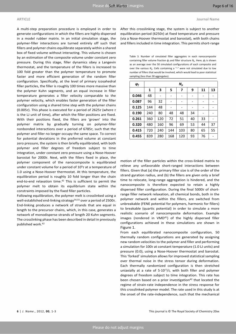
Table 3. Number of simulated filler aggregates in each nanocomposite containing filler volume fraction ϕf and filler structure Np. Here, ϕf is shown as an average over the 50 simulated configurations of each composite and over the various Np. Cells containing a “-“ were not simulated due to low number of fillers that would be involved, which would lead to poor statistical sampling (less than 30 aggregates).

ϕf Np

1 3 5 7 9 11 130.046 48 - - - - - -0.087 96 32 - - - - -0.125 144 48 - - - - -0.190 240 80 48 48 34 - -0.261 360 120 72 51 40 33 -0.320 480 160 96 69 53 44 370.415 720 240 144 103 80 65 550.455 839 280 168 120 93 76 -


Soft Matter ARTICLE




response at the chosen strain rate is dominated primarily by the rubbery plateau rather than by high-frequency dynamics. Constant zero pressure boundary conditions are imposed in the directions normal to deformation using a Nose-Hoover barostat. This allows the normal dimensions to respond dynamically to the imposed strain, as would be expected in a traditional tensile test in which a sample’s volume is set by its Poisson ratio.

Results

The

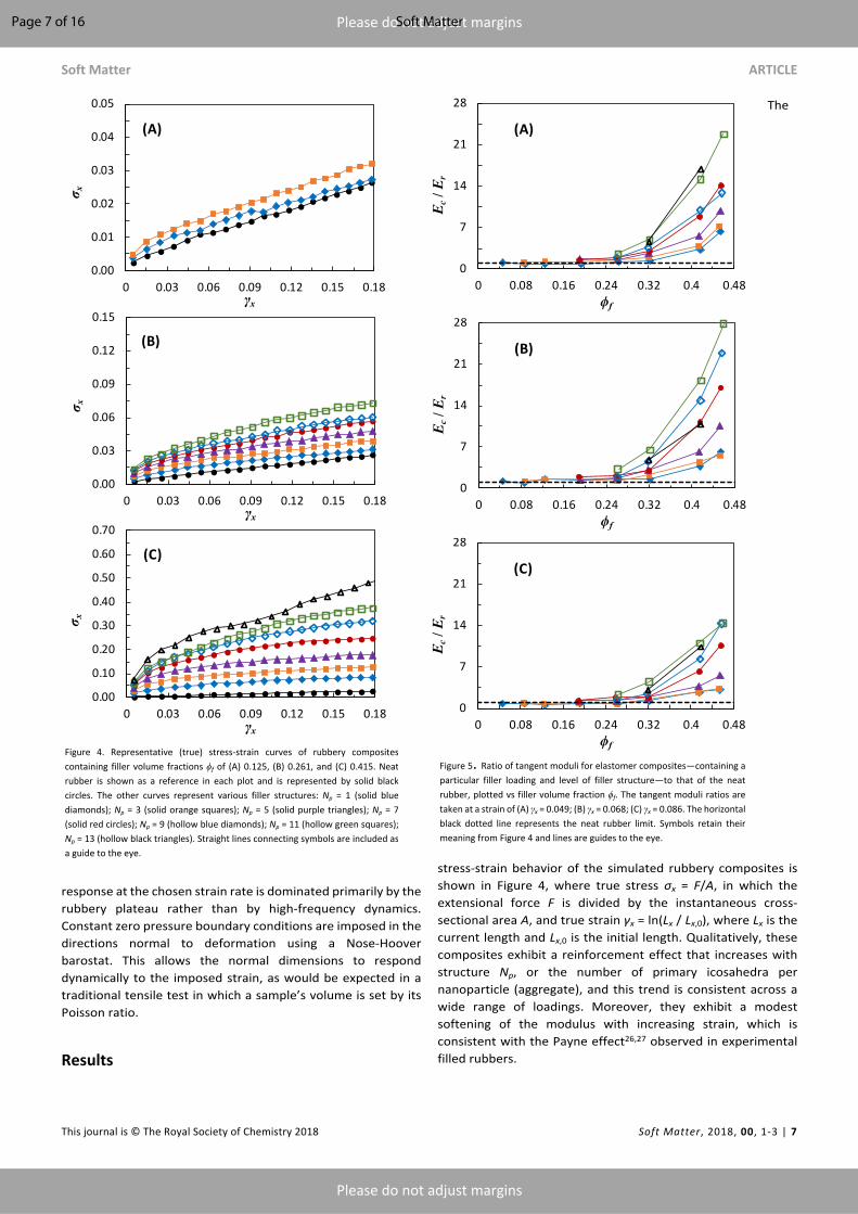
stress-strain behavior of the simulated rubbery composites is shown in Figure 4, where true stress σx = F/A, in which the extensional force F is divided by the instantaneous cross-sectional area A, and true strain γx = ln(Lx / Lx,0), where Lx is the current length and Lx,0 is the initial length. Qualitatively, these composites exhibit a reinforcement effect that increases with structure Np, or the number of primary icosahedra per nanoparticle (aggregate), and this trend is consistent across a wide range of loadings. Moreover, they exhibit a modest softening of the modulus with increasing strain, which is consistent with the Payne effect26,27 observed in experimental filled rubbers.

Figure 5. Ratio of tangent moduli for elastomer composites—containing a particular filler loading and level of filler structure—to that of the neat rubber, plotted vs filler volume fraction ϕf. The tangent moduli ratios are taken at a strain of (A) γx = 0.049; (B) γx = 0.068; (C) γx = 0.086. The horizontal black dotted line represents the neat rubber limit. Symbols retain their meaning from Figure 4 and lines are guides to the eye.

0

7

14

21

28

0 0.08 0.16 0.24 0.32 0.4 0.48

E c/ E

r

ϕf

(C)

0

7

14

21

28

0 0.08 0.16 0.24 0.32 0.4 0.48

E c/ E

r

ϕf

(B)

0

7

14

21

28

0 0.08 0.16 0.24 0.32 0.4 0.48

E c/ E

r

ϕf

(A)

Figure 4. Representative (true) stress-strain curves of rubbery composites containing filler volume fractions ϕf of (A) 0.125, (B) 0.261, and (C) 0.415. Neat rubber is shown as a reference in each plot and is represented by solid black circles. The other curves represent various filler structures: Np = 1 (solid blue diamonds); Np = 3 (solid orange squares); Np = 5 (solid purple triangles); Np = 7 (solid red circles); Np = 9 (hollow blue diamonds); Np = 11 (hollow green squares); Np = 13 (hollow black triangles). Straight lines connecting symbols are included as a guide to the eye.

0.00

0.01

0.02

0.03

0.04

0.05

0 0.03 0.06 0.09 0.12 0.15 0.18

σ x

γx

(A)

0.00

0.03

0.06

0.09

0.12

0.15

0 0.03 0.06 0.09 0.12 0.15 0.18

σ x

γx

(B)

0.00

0.10

0.20

0.30

0.40

0.50

0.60

0.70

0 0.03 0.06 0.09 0.12 0.15 0.18

σ x

γx

(C)






In order to better quantify this reinforcement effect, we compute the instantaneous (tangent) composite moduli Ec. As shown in Figure 5A-C, the extensional modulus exhibits a strongly nonlinear enhancement with increasing filler content, with more structured nanoparticles yielding greater reinforcement at fixed nanoparticle loading. These data are qualitatively comparable to trends in reinforcement observed in experimental rubber/nanofiller composites.56,57 Notably, the extensional moduli increase by as much as a factor of 10-20 relative to the neat rubber, particularly in highly loaded composites containing highly structured fillers. The observed increase is much greater than early predictions of modulus enhancement from the Einstein or Guth equations. What is this origin of this large reinforcement effect? Test of occluded rubber hypothesis

We first test the long-standing proposition, summarized in the introduction, that the formation of non-deforming rubber

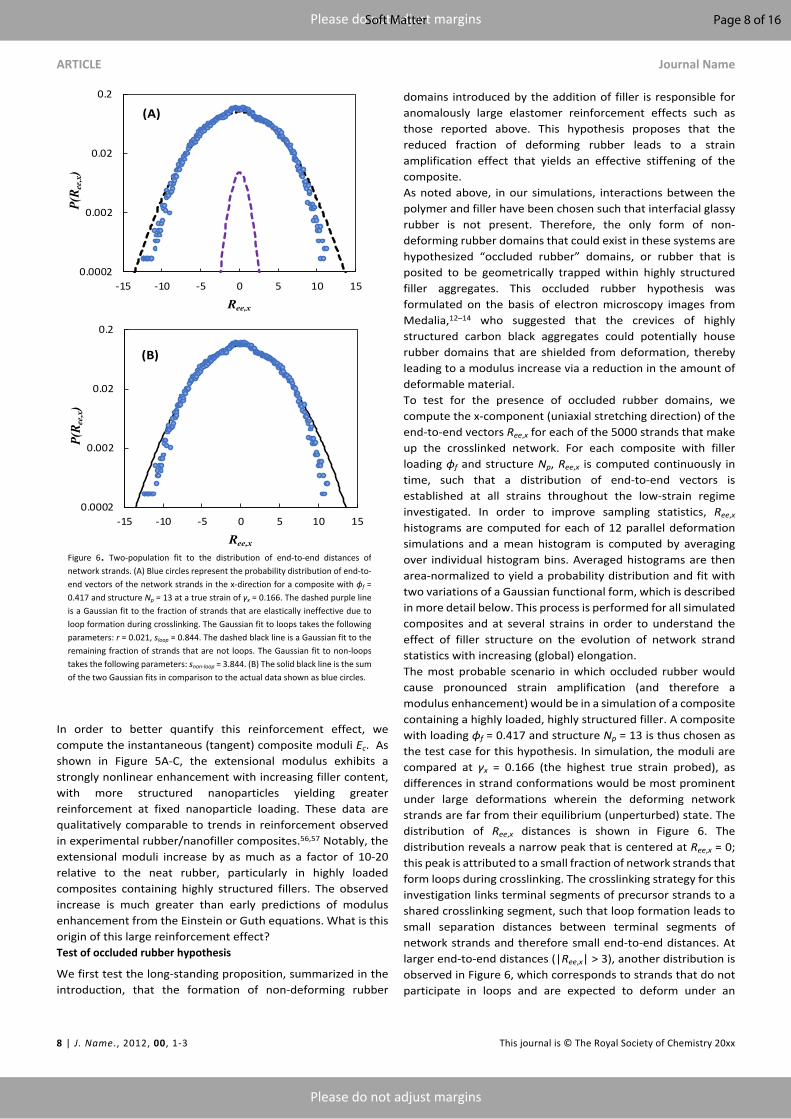
domains introduced by the addition of filler is responsible for anomalously large elastomer reinforcement effects such as those reported above. This hypothesis proposes that the reduced fraction of deforming rubber leads to a strain amplification effect that yields an effective stiffening of the composite.As noted above, in our simulations, interactions between the polymer and filler have been chosen such that interfacial glassy rubber is not present. Therefore, the only form of non-deforming rubber domains that could exist in these systems are hypothesized “occluded rubber” domains, or rubber that is posited to be geometrically trapped within highly structured filler aggregates. This occluded rubber hypothesis was formulated on the basis of electron microscopy images from Medalia,12–14 who suggested that the crevices of highly structured carbon black aggregates could potentially house rubber domains that are shielded from deformation, thereby leading to a modulus increase via a reduction in the amount of deformable material. To test for the presence of occluded rubber domains, we compute the x-component (uniaxial stretching direction) of the end-to-end vectors Ree,x for each of the 5000 strands that make up the crosslinked network. For each composite with filler loading ϕf and structure Np, Ree,x is computed continuously in time, such that a distribution of end-to-end vectors is established at all strains throughout the low-strain regime investigated. In order to improve sampling statistics, Ree,x histograms are computed for each of 12 parallel deformation simulations and a mean histogram is computed by averaging over individual histogram bins. Averaged histograms are then area-normalized to yield a probability distribution and fit with two variations of a Gaussian functional form, which is described in more detail below. This process is performed for all simulated composites and at several strains in order to understand the effect of filler structure on the evolution of network strand statistics with increasing (global) elongation.The most probable scenario in which occluded rubber would cause pronounced strain amplification (and therefore a modulus enhancement) would be in a simulation of a composite containing a highly loaded, highly structured filler. A composite with loading ϕf = 0.417 and structure Np = 13 is thus chosen as the test case for this hypothesis. In simulation, the moduli are compared at γx = 0.166 (the highest true strain probed), as differences in strand conformations would be most prominent under large deformations wherein the deforming network strands are far from their equilibrium (unperturbed) state. The distribution of Ree,x distances is shown in Figure 6. The distribution reveals a narrow peak that is centered at Ree,x = 0; this peak is attributed to a small fraction of network strands that form loops during crosslinking. The crosslinking strategy for this investigation links terminal segments of precursor strands to a shared crosslinking segment, such that loop formation leads to small separation distances between terminal segments of network strands and therefore small end-to-end distances. At larger end-to-end distances (|Ree,x| > 3), another distribution is observed in Figure 6, which corresponds to strands that do not participate in loops and are expected to deform under an

Figure 6. Two-population fit to the distribution of end-to-end distances of network strands. (A) Blue circles represent the probability distribution of end-to-end vectors of the network strands in the x-direction for a composite with ϕf = 0.417 and structure Np = 13 at a true strain of γx = 0.166. The dashed purple line is a Gaussian fit to the fraction of strands that are elastically ineffective due to loop formation during crosslinking. The Gaussian fit to loops takes the following parameters: r = 0.021, sloop = 0.844. The dashed black line is a Gaussian fit to the remaining fraction of strands that are not loops. The Gaussian fit to non-loops takes the following parameters: snon-loop = 3.844. (B) The solid black line is the sum of the two Gaussian fits in comparison to the actual data shown as blue circles.

0.0002

0.002

0.02

0.2

-15 -10 -5 0 5 10 15

P(R e

e,x)

Ree,x

(A)

0.0002

0.002

0.02

0.2

-15 -10 -5 0 5 10 15

P(R e

e,x)

Ree,x

(B)


Soft Matter ARTICLE




imposed global composite extension. In analyzing this data, we assume Gaussian chain statistics, such that the total probability distribution P(Ree,x) of end-to-end distances can be represented as the sum of two Gaussian probability distributions:

(20)

2

,, 2

2

,

2

1exp22

1 1exp22

ee xee x

looploop

ee x

defdef

RrP Rss

Rrss

where the first term represents a Gaussian distribution for loops, and the second term represents a Gaussian distribution for the deforming strands (the remaining strands that are non-loops). In equation (20), r is the fraction of network strands participating in loops, sloop is the standard deviation of the Gaussian fit to the population of loops, and sdef is the standard deviation of the Gaussian fit to the population of deforming network strands. Since the fraction of strands that participate in loops is constant (no new loops form during extension) and the loops are non-deforming, the values of r and sloop are pre-determined at all non-zero strains by using their respective fit values obtained to a fit at zero-strain (before deformation). The standard deviation of the deforming strand population sdef is left as a free parameter since it is dependent on the global composite strain.

The individual fits to the non-deforming loop population and deforming strands population are shown in Figure 6A. The value of r is 0.021, which suggests that the fraction of strands participating in loops is small – of order a few percent. The total (summed) fit to the distribution is shown in Figure 6B. The total fit is in excellent agreement with the data for distances |Ree,x| less than 8-10. The disagreement between the fit and data in the tails of the distribution is a consequence of the finite extensibility of real polymer chains; the Gaussian approximation over-predicts the probability of very large end-to-end distances. Nevertheless, the breakdown of the two-term (total) Gaussian fit occurs beyond two standard deviations of the deforming strand population fit (sdef = 3.844). Therefore, the supposition of two populations of network strands (non-deforming loops and deforming strands) is highly representative of the distribution of end-to-end vectors. If occluded rubber were the primary origin for the observed reinforcement in the composites with highly structured fillers, then a successful fit to these data would require a third population of strands. In addition to a population of deforming strands and a small population of non-deforming loops, there would also exist a population of non-deforming ‘occluded’ network strands. Thus, under the occluded rubber hypothesis, the total probability distribution of end-to-end vectors would be represented with the following functional form:

(21)

2

,, 2

2

,

2

2,

2

1exp22

1exp22

1 1exp22

loop ee xee x

looploop

def ee x

defdef

loop def ee x

occocc

r RP R

ss

r Rss

r r Rss

Here, the first term represents the population of non-deforming loops, the second term represents the population of deforming network strands, and the third term represents the population of non-deforming, occluded strands. For clarity, discussions will use the following notation for these fits: the Gaussian fit to the loop population is Gloop (which adopts a pre-determined loop fraction rloop and standard deviation sloop from the zero strain, 2-term Gaussian fit previously discussed), the Gaussian fit to the deforming rubber population is Gdef (with a deforming rubber fraction equal to rdef and standard deviation sdef;), and the Gaussian fit to the occluded rubber population is Gocc (with an occluded rubber fraction equal to (1 – rloop – rdef) and standard deviation socc equal to the zero-strain standard deviation of the population of non-loops).As described above, within the occluded rubber hypothesis, filled elastomers are argued to possess a (loading dependent) fraction of non-deforming rubber sufficient to yield the observed modulus as a consequence of strain amplification within a series (iso-stress) model. This approach is commonly used to ‘correct’ the Guth equation, which predicts the modulus enhancement as a function of filler loading:

(22)214.1 2.5 1c r eff effE E

where Ec and Er are the composite and neat rubber tangent extensional modulus, and eff is an effective filler volume fraction, taken as the sum of the true filler volume fraction and an occluded rubber fraction occ. Here, occluded rubber is treated as a fitting parameter, which is adjusted to achieve agreement between the Guth equation and measured moduli. In order to test this hypothesis, we thus first back-calculate the value of ϕocc inferred by this approach. At γx = 0.166, the composite modulus is 16.4 times greater than the neat rubber modulus. In order for the Guth equation to capture a moduli ratio of 16.4, an effective filler loading of eff = 0.961 would be required. With a true filler loading = 0.417, the occluded rubber fraction occ of the total composite would be 0.544. This hypothesis therefore anticipates that only 3.9% of the composite (or 6.7% of the rubber fraction of the composite) would be responsible for all deformation. We thus employ these fractions to obtain the r values in equation (21): 6.7% of the strands are treated as deforming; the fraction of loops is assumed to remain constant from the previous (two-population) assessment (rloop = 0.021 and sloop = 0.844) since the choice of hypothesis (two populations vs three populations of strands) has no influence on the crosslinking behavior; and the remaining fraction of strands are treated as occluded. The






standard deviation of the occluded strands socc is held constant with elongation to reflect the posited non-participation of these strands in deformation and is taken as the standard deviation of the distribution of non-loops at zero-strain (unperturbed) from the two-term Gaussian fit (which gives a value of socc = 3.23). The standard deviation of the deforming rubber distribution sdef is determined as follows: at a true (global composite) strain of γx = 0.166, the engineering strain γe is 0.18. Since only 3.9% of the material in the composite is deformable under the occluded rubber hypothesis, the deforming strands experience an amplified engineering strain equal to γe = 0.18/0.039 = 4.56. Thus, when the composite is extended to an engineering strain

of 0.18, the average length of the deforming strands at this global strain, recalling that the average zero-strain (unperturbed) strand length Ree,x0 = 3.23, must be Ree,x = 17.9 if this model is to account for the observed overall modulus. A value of 17.9 is thus employed for the standard deviation of the deforming (and highly strain amplified) population sdef. The results for this three-population model are shown in Figure 7. This model evidently underpredicts the end-to-end distance at low/medium strand lengths, and overpredicts the end-to-end distance at high strand length (in the distribution tails). Overall, the data suggest that there is not an appreciable population of non-deforming rubber beyond covalent loops, nor is there a

Figure 7. Three-population fit to the distribution of end-to-end distances of network strands as predicted by the occluded rubber hypothesis. (a) Blue circles represent the probability distribution of end-to-end vectors of the network strands in the x-direction for a composite with ϕf = 0.417 and structure Np = 13 at a true strain of γx = 0.166. The dashed purple line is a Gaussian fit to the fraction of strands that are elastically ineffective due to loop formation during crosslinking. The Gaussian fit to loops takes the following parameters: r = 0.021, sloop = 0.844. These parameters are identical to the two-term fit parameters for the loop population. The black dashed line represents the hypothesize occluded rubber population, with an occluded rubber fraction of 0.916 and standard deviation socc = 3.23. The green dashed line represents the Gaussian fit to the deforming population of network strands. The fraction of deforming strands rdef = 0.067 and the standard deviation of the distribution of deforming strands is sdef = 17.9. (b) the black solid line is the total 3-population fit (sum of all population fits from (a)) relative to the actual data, shown as blue circles.

0.0002

0.002

0.02

0.2

-15 -10 -5 0 5 10 15

P(R e

e,x)

Ree,x

(A)

0.0002

0.002

0.02

0.2

-15 -10 -5 0 5 10 15

P(R e

e,x)

Ree,x

(B)

Figure 8. Poisson ratio as a function of strain for the nanocomposites with filler loadings ϕf of (A) 0.125, (B) 0.261, and (C) 0.415. Symbols represent varying degrees of structure Np and retain their meaning from Figure 5. Straight lines between symbols are a guide to the eye. The horizontal black dotted line corresponds to the limit of volume conservation during deformation.

0.41

0.44

0.47

0.50

0 0.03 0.06 0.09 0.12 0.15 0.18

ν

γx

(A)

0.41

0.44

0.47

0.50

0 0.03 0.06 0.09 0.12 0.15 0.18

ν

γx

(B)

0.41

0.44

0.47

0.50

0 0.03 0.06 0.09 0.12 0.15 0.18

ν

γx

(C)


Soft Matter ARTICLE




small population of highly strain amplified, deforming rubber. These distributions of end-to-end strand lengths indicate that these model systems contain no population of non-deforming rubber beyond network defects. Evidently, the occluded rubber hypothesis does not explain the modulus enhancement in these simulated elastomeric nanocomposites.Reinforcement by Poisson ratio mismatch

We next test the hypothesis, quantified by equation (12), that the Poisson ratio mismatch between the rubber matrix and a jammed filler network leads to reinforcement of the extensional modulus by a fraction of the matrix bulk modulus. To do so, we first consider whether the Poisson ratio of these composites

behaves in the manner anticipated by this theory: enhancements in modulus should generally accompany a reduction in composite Poisson ratio. In Figure 8, the Poisson ratio is plotted as a function of elongational strain for the same nanocomposites for which stress-strain curves were shown in Figure 4. Similar to the trend in extensional modulus, for a given loading, there exists a monotonic trend in the Poisson ratio suppression with structure Np: as structure increases, the Poisson ratio of the rubbery composite decreases. This trend becomes more pronounced at higher loadings. When we replot these data in Figure 9 to show the filler-loading-dependence of the Poisson ratio at fixed strain, a striking similarity emerges with the corresponding modulus enhancement shown in Figure 5. As the composite modulus increases, the composite Poisson ratio is increasingly suppressed below ν = 0.5, the ideal limit of volume conservation under deformation (which is the typical assumption for ν in neat rubber). At low loadings, the Poisson ratio nearly obeys the expected value for neat rubber, and the extensional modulus does not see appreciable reinforcement. However, at higher loadings, particularly with higher structures, the Poisson ratio is reduced to values as low as 0.44, and this drop in Poisson ratio is accompanied by substantial enhancement in the extensional modulus. Put another way, the composites undergo greater volume growth on extension in more highly reinforced (greater extensional modulus) cases. In order to more quantitatively test the relationship between Poisson ratio suppression and enhanced modulus predicted by equation (12), we must first obtain values for the strain amplification factor f in equation (12). The value of f should in general be bounded between one and the series model prediction of one over the rubber volume fraction. Instead of relying upon either of these models, here we employ data directly from the end-to-end vector analysis described above. Specifically, we define a molecular-level polymer strain as

(23),

,

, ,0

lnee x

ee xR

ee x

RR

where Ree,x is the x-component of the end-to-end vector of a network strand at some non-zero global strain (i.e. after mechanical deformation has started), Ree,x,0 is the x-component of the end-to-end vector of a network strand at time t = 0 (before stretching), and angle brackets indicate an ensemble average. For each filled system, a strain amplification factor f is computed by taking the ratio of the molecular strain in the composite (at a particular global strain) to the molecular strain in the neat rubber (at the same global strain):

(24),

, ,

ee x

ee x neat

R

R

f

Representative strain-amplification factors as a function of global strain are shown in Figure 10A. For a given composite, f is roughly constant in strain, which is to be expected within the linear regime. To capture the general behavior throughout this regime, we employ a strain averaged value of f, in which an average of f over the range γx = 4-18% is used to compute a mean

Figure 9. Poisson ratios of the same systems shown in Figure 5 as a function of ϕf. The Poisson ratios are taken at a strain of (A) γx = 0.049; (B) γx = 0.068; (C) γx = 0.086. The horizontal black line in each plot represents the ideal limit of volume conservation (ν = 0.5).

0.42

0.44

0.46

0.48

0.5

0.52

0 0.08 0.16 0.24 0.32 0.4 0.48

ν

ϕf

(A)

0.42

0.44

0.46

0.48

0.5

0.52

0 0.08 0.16 0.24 0.32 0.4 0.48

ν

ϕf

(B)

0.42

0.44

0.46

0.48

0.5

0.52

0 0.08 0.16 0.24 0.32 0.4 0.48

ν

ϕf

(C)






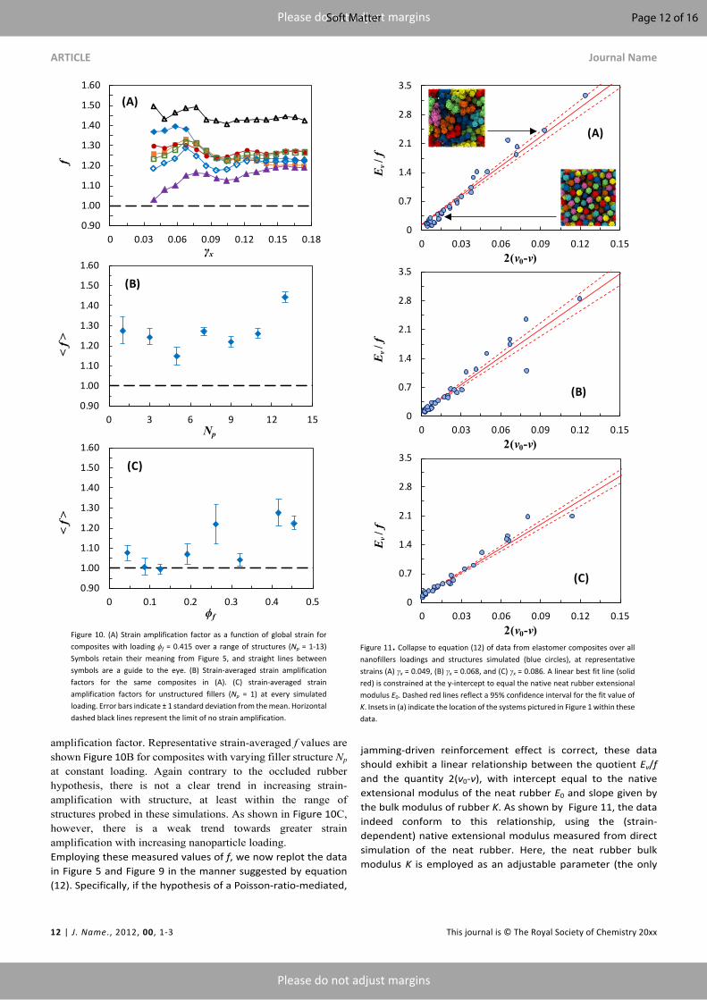
amplification factor. Representative strain-averaged f values are shown Figure 10B for composites with varying filler structure Np at constant loading. Again contrary to the occluded rubber hypothesis, there is not a clear trend in increasing strain-amplification with structure, at least within the range of structures probed in these simulations. As shown in Figure 10C, however, there is a weak trend towards greater strain amplification with increasing nanoparticle loading.Employing these measured values of f, we now replot the data in Figure 5 and Figure 9 in the manner suggested by equation (12). Specifically, if the hypothesis of a Poisson-ratio-mediated,

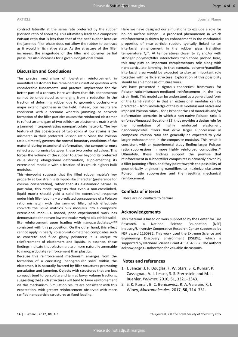
jamming-driven reinforcement effect is correct, these data should exhibit a linear relationship between the quotient Eν/f and the quantity 2(ν0-ν), with intercept equal to the native extensional modulus of the neat rubber E0 and slope given by the bulk modulus of rubber K. As shown by Figure 11, the data indeed conform to this relationship, using the (strain-dependent) native extensional modulus measured from direct simulation of the neat rubber. Here, the neat rubber bulk modulus K is employed as an adjustable parameter (the only

Figure 10. (A) Strain amplification factor as a function of global strain for composites with loading ϕf = 0.415 over a range of structures (Np = 1-13) Symbols retain their meaning from Figure 5, and straight lines between symbols are a guide to the eye. (B) Strain-averaged strain amplification factors for the same composites in (A). (C) strain-averaged strain amplification factors for unstructured fillers (Np = 1) at every simulated loading. Error bars indicate ± 1 standard deviation from the mean. Horizontal dashed black lines represent the limit of no strain amplification.

0.90

1.00

1.10

1.20

1.30

1.40

1.50

1.60

0 0.03 0.06 0.09 0.12 0.15 0.18

f

γx

(A)

0.90

1.00

1.10

1.20

1.30

1.40

1.50

1.60

0 3 6 9 12 15

< f >

Np

(B)

0.90

1.00

1.10

1.20

1.30

1.40

1.50

1.60

0 0.1 0.2 0.3 0.4 0.5

< f >

ϕf

(C)

Figure 11. Collapse to equation (12) of data from elastomer composites over all nanofillers loadings and structures simulated (blue circles), at representative strains (A) γx = 0.049, (B) γx = 0.068, and (C) γx = 0.086. A linear best fit line (solid red) is constrained at the y-intercept to equal the native neat rubber extensional modulus E0. Dashed red lines reflect a 95% confidence interval for the fit value of K. Insets in (a) indicate the location of the systems pictured in Figure 1 within these data.

0

0.7

1.4

2.1

2.8

3.5

0 0.03 0.06 0.09 0.12 0.15

E ν/ f

2(ν0-ν)

(A)

0

0.7

1.4

2.1

2.8

3.5

0 0.03 0.06 0.09 0.12 0.15

E ν/ f

2(ν0-ν)

(C)

0

0.7

1.4

2.1

2.8

3.5

0 0.03 0.06 0.09 0.12 0.15

E ν/ f

2(ν0-ν)

(B)


Soft Matter ARTICLE




adjustable parameter in the model). Are the resulting fit values consistent with the bulk modulus of the neat rubber? To answer this question, the fit values of K must be compared to the zero-strain (i.e. equilibrium) bulk modulus K0 of the neat rubber. To make this comparison, we compute the equilibrium bulk modulus in another set of simulations from the fluctuation-dissipation theorem for isothermal compressibility, which relates the compressibility (and therefore the bulk modulus) to fluctuations in system volume at fixed particle number:58

(25)22

VK kT

V V

where V is the volume, k and T are the Boltzmann constant and temperature, respectively, and brackets indicate an ensemble or long-time average. This determination is made from quiescent simulations held at constant pressure employing a Nose-Hoover thermostat and barostat, which yields fluctuations consistent with the canonical ensemble.59 The temperature T and pressure P are damped every 2τ, and the instantaneous volume is measured every 25τ. The comparison between the zero-strain bulk modulus K0 and the fit values of K is shown over a range of strains in Figure 12. This comparison is complicated by the fact that K0 is computed in an unperturbed system, whereas the fit values of the bulk moduli describe the resistance of the system to volume deformation after some nonzero combination of both elongational and volume strain. Nevertheless, the resulting strain-dependent fit values of K recover the zero-strain neat rubber bulk modulus at all strains below ~8%. Beyond 8%, an observed strain-softening in the fit values of K can be understood from the expected reduction in the density of van der Waals interactions as the rubber’s density drops in filled elastomers with Poisson ratio less than 0.5 and its molecular packing is perturbed from its equilibrium state. These findings support a scenario wherein a jammed filler network forces a reduction in the composite Poisson ratio from its rubber-preferred value of nearly ½. The resulting growth in

rubber volume with strain leads to an enhancement of the composite elongational modulus by a portion of the rubber bulk modulus, with some strain-softening of the bulk modulus modestly weakening this effect at higher strains. Direct evidence of reinforcement driven by a Poisson ratio mismatch between the rubber and jammed filler is provided in Figure 13. In the y-direction (normal to the stretching direction), a stress balance develops between the polymer and jammed filler in which the partial stresses within the two phases offset one another in order to maintain constant zero normal stress. The partial pressure of the filler ∆pyy, filler increases monotonically with elongational strain, while the partial pressure of the polymer ∆pyy, poly is opposite in sign and roughly equal in magnitude to ∆pyy, filler. In other words, during uniaxial extension, the jammed filler network pushes outward against contractile tension emerging from the rubber matrix’s bulk modulus. The reason for this behavior can be explained from the perspective of the Poisson ratio: jammed filler deforms with a Poisson ratio of about one-third, and therefore does not

-0.20

-0.15

-0.10

-0.05

0.00

0 0.03 0.06 0.09 0.12 0.15 0.18

∆pyy

, pol

y

γx

0.00

0.05

0.10

0.15

0.20

0 0.03 0.06 0.09 0.12 0.15 0.18

∆pyy

, fill

er

γx

(A)

(B)

Figure 13. Partial pressure along the y-dimension of the (a) filler and (b) polymer in a highly loaded (ϕf = 0.415) rubbery composite. The y-dimension is orthogonal to the direction of elongation (x-direction). Symbols retain their meaning from Figure 5, and straight lines connecting symbols are a guide to the eye.

0

5

10

15

20

25

0 0.03 0.06 0.09 0.12 0.15 0.18

K

γx

Figure 12. Fit values for the rubber bulk modulus K (blue diamonds) as a function of strain at which the collapse from Figure 11 is performed, compared to the zero-strain (equilibrium) neat rubber bulk modulus obtained by direct measurement (red circle). Error bars on all data points indicate 95% confidence intervals for the values of K.






contract laterally at the same rate preferred by the rubber (Poisson ratio of about ½). This ultimately leads to a composite Poisson ratio that is less than that of the neat rubber because the jammed filler phase does not allow the rubber to contract as it would in its native state. As the structure of the filler increases, the magnitude of the filler and polymer partial pressures also increases for a given elongational strain.

Discussion and ConclusionsThe precise mechanism of low-strain reinforcement in nanofilled elastomers has remained an unsettled question with considerable fundamental and practical implications for the better part of a century. Here we show that this phenomenon cannot be understood as emerging from a reduction in the fraction of deforming rubber due to geometric occlusion– a major extant hypothesis in the field. Instead, our results are consistent with a scenario wherein jamming or network formation of the filler particles causes the reinforced elastomer to reflect an amalgam of two solids – an elastomeric matrix with a jammed interpenetrating nanoparticulate network. The key feature of this coexistence of two solids at low strains is the mismatch in their preferred Poisson ratio. Since the Poisson ratio ultimately governs the normal boundary conditions of the material during extensional deformation, the composite must reflect a compromise between these two preferred values. This forces the volume of the rubber to grow beyond its preferred value during elongational deformation, supplementing its extensional modulus with a fraction of its (much higher) bulk modulus. This viewpoint suggests that the filled rubber matrix’s key property at low strain is its liquid-like character (preference for volume conservation), rather than its elastomeric nature. In particular, this model suggests that even a non-crosslinked, liquid matrix should yield a solid-like extensional response under high filler loading – a predicted consequence of a Poisson ratio mismatch with the jammed filler, which effectively converts the liquid matrix’s bulk modulus into a composite extensional modulus. Indeed, prior experimental work has demonstrated that even low molecular-weight oils exhibit solid-like reinforcement upon loading with nanoparticulates,23,60 consistent with this proposition. On the other hand, this effect cannot apply in nearly Poisson-ratio-matched composites such as concrete and filled glassy polymers; it is unique to reinforcement of elastomers and liquids. In essence, these findings indicate that elastomers are more naturally amenable to nanoparticulate reinforcement than plastics. Because this reinforcement mechanism emerges from the formation of a coexisting ‘nanogranular solid’ within the elastomer, it is naturally favored by filler structures promoting percolation and jamming. Objects with structures that are less compact tend to percolate and jam at lower volume fractions, suggesting that such structures will tend to favor reinforcement via this mechanism. Simulation results are consistent with this expectation, with greater reinforcement observed with more rarified nanoparticle structures at fixed loading.

Here we have designed our simulations to exclude a role for bound surface rubber – a proposed phenomenon in which reinforcement is driven by an enhancement in the mechanical properties of near-particle rubber, typically linked to an interfacial enhancement in the rubber glass transition temperature Tg

15. At temperatures closer to Tg and/or with stronger polymer/filler interactions than those probed here, this may play an important complementary role along with nanoparticulate jamming. In that scenario, polymer/nanofiller interfacial area would be expected to play an important role together with particle structure. Exploration of this possibility should be an emphasis of future work.We have presented a rigorous theoretical framework for Poisson-ratio-mismatch-mediated reinforcement in the low strain limit. This model can be understood as a generalized form of the Lamé relation in that an extensional modulus can be predicted – from knowledge of the bulk modulus and native and imposed Poisson ratios – for a broader class of materials and/or deformation scenarios in which a non-native Poisson ratio is enforced/imposed. Equation (12) thus provides a design rule for the formulation of highly reinforced elastomeric nanocomposites: fillers that drive larger suppressions in composite Poisson ratio can generally be expected to yield larger enhancements in the composite modulus. This result is consistent with an experimental study finding larger Poisson ratio suppressions in more highly reinforced composites.39 Ultimately, these findings support the premise that reinforcement in rubber/filler composites is primarily driven by a filler jamming effect, and they point towards the possibility of geometrically engineering nanofillers to maximize elastomer Poisson ratio suppression and the resulting mechanical reinforcement.

Conflicts of interest There are no conflicts to declare.

AcknowledgementsThis material is based on work supported by the Center for Tire Research, a National Science Foundation (NSF) Industry/University Cooperative Research Center supported by NSF award 1160982. This work used the Extreme Science and Engineering Discovery Environment (XSEDE), which is supported by National Science Grant ACI-1548562. The authors acknowledge C. Robertson for valuable discussions.

Notes and references1 J. Jancar, J. F. Douglas, F. W. Starr, S. K. Kumar, P.

Cassagnau, A. J. Lesser, S. S. Sternstein and M. J. Buehler, Polymer, 2010, 51, 3321–3343.

2 S. K. Kumar, B. C. Benicewicz, R. A. Vaia and K. I. Winey, Macromolecules, 2017, 50, 714–731.


Soft Matter ARTICLE




3 Q. Wang, R. Hou, Y. Cheng and J. Fu, Soft Matter, 2012, 8, 6048–6056.

4 Y. Tanaka, J. P. Gong and Y. Osada, Prog. Polym. Sci., 2005, 30, 1–9.

5 A. Einstein, Ann. Phys., 1906, 324, 289–306.6 Smallwood, H.M., J. Appl. Phys., 1944, 15, 758–766.7 E. Guth, Rubber Chem. Technol., 1945, 18, 596–604.8 E. M. Dannenberg, Rubber Chem. Technol., 1986, 59,

512–524.9 M.-J. Wang, Rubber Chem. Technol., 1998, 71, 520–

589.10 G. Heinrich, M. Klüppel and T. A. Vilgis, Curr. Opin.

Solid State Mater. Sci., 2002, 6, 195–203.11 V. Pryamitsyn and V. Ganesan, Macromolecules,

2006, 39, 844–856.12 A. I. Medalia, Rubber Chem. Technol., 1972, 45,

1171–1194.13 A. I. Medalia, Rubber Chem. Technol., 1973, 46, 877–

896.14 A. I. Medalia, Rubber Chem. Technol., 1974, 47, 411–

433.15 D. S. Simmons, Macromol. Chem. Phys., 2016, 217,

137–148.16 S. Napolitano, E. Glynos and N. B. Tito, Rep. Prog.

Phys., 2017, 80, 036602.17 C. G. Robertson and C. M. Roland, Rubber Chem.

Technol., 2008, 81, 506–522.18 R. B. Bogoslovov, C. M. Roland, A. R. Ellis, A. M.

Randall and C. G. Robertson, Macromolecules, 2008, 41, 1289–1296.

19 Y. Liu, L. Li and Q. Wang, J. Appl. Polym. Sci., 2010, 118, 1111–1120.

20 X. Wang and C. G. Robertson, Phys. Rev. E, 2005, 72, 031406.

21 S. Richter, M. Saphiannikova, K. W. Stöckelhuber and G. Heinrich, Macromol. Symp., 2010, 291–292, 193–201.

22 C. G. Robertson and X. Wang, EPL Europhys. Lett., 2006, 76, 278.

23 C. G. Robertson and X. Wang, Phys. Rev. Lett., 2005, 95, 075703.

24 S. Richter, H. Kreyenschulte, M. Saphiannikova, T. Götze and G. Heinrich, Macromol. Symp., 2011, 306–307, 141–149.

25 C. M. Roland, Rubber Chem. Technol., 2015, 89, 32–53.

26 W. P. Fletcher and A. N. Gent, Rubber Chem. Technol., 1954, 27, 209–222.

27 A. R. Payne, J. Appl. Polym. Sci., 1962, 6, 57–63.28 T. Akçaoğlu, M. Tokyay and T. Çelik, Cem. Concr.

Compos., 2004, 26, 633–638.

29 Z. Qian, E. J. Garboczi, G. Ye and E. Schlangen, Mater. Struct., 2016, 49, 149–158.

30 P. Stroeven and Z.-Q. Guo, in Advances in Construction Materials 2007, Springer, Berlin, Heidelberg, 2007, pp. 757–764.

31 N. W. Tschoegl, W. G. Knauss and I. Emri, Mech. Time-Depend. Mater., 2002, 6, 3–51.

32 R. S. Lakes and A. Wineman, J. Elast., 2006, 85, 45–63.

33 P. J. Flory, Polymer, 1979, 20, 1317–1320.34 M. Rubinstein, Polymer Physics, Oxford University

Press, 2003.35 P. H. Mott and C. M. Roland, Phys. Rev. B, 2009, 80,

132104.36 G. N. Greaves, A. L. Greer, R. S. Lakes and T. Rouxel,

Nat. Mater., 2011, 10, 823–837.37 T. Rouxel, H. Ji, T. Hammouda and A. Moréac, Phys.

Rev. Lett., 2008, 100, 225501.38 J. Schroers and W. L. Johnson, Phys. Rev. Lett., 2004,

93, 255506.39 C. G. Robertson, R. Bogoslovov and C. M. Roland,

Phys. Rev. E, 2007, 75, 051403.40 B. P. Holownia, Rubber Chem. Technol., 1975, 48,

246–253.41 W. Humphrey, A. Dalke and K. Schulten, J. Mol.

Graph., 1996, 14, 33–38.42 S. M. Smith and D. S. Simmons, Rubber Chem.

Technol., 2017, 90, 238–263.43 G. S. Grest and K. Kremer, Phys. Rev. A, 1986, 33,

3628.44 M. Pütz, K. Kremer and G. S. Grest, EPL Europhys.

Lett., 2000, 49, 735.45 J. Rottler, S. Barsky and M. O. Robbins, Phys. Rev.

Lett., 2002, 89, 148304.46 T. Ge, F. Pierce, D. Perahia, G. S. Grest and M. O.

Robbins, Phys. Rev. Lett., 2013, 110, 098301.47 S. Plimpton, J. Comput. Phys., 1995, 117, 1–19.48 B. A. P. Betancourt, J. F. Douglas and F. W. Starr, Soft

Matter, 2012, 9, 241–254.49 J. H. Mangalara and D. S. Simmons, ACS Macro Lett.,

2015, 1134–1138.50 P. Z. Hanakata, J. F. Douglas and F. W. Starr, J. Chem.

Phys., 2012, 137, 244901.51 W. L. Merling, J. B. Mileski, J. F. Douglas and D. S.

Simmons, Macromolecules, 2016, 49, 7597–7604.52 R. J. Lang and D. S. Simmons, Macromolecules, 2013,

46, 9818–9825.53 M. P. Allen and D. J. Tildesley, Computer Simulation

of Liquids; Oxford Univ. Press, Oxford, 1987.54 E. R. Duering, K. Kremer and G. S. Grest, J. Chem.

Phys., 1994, 101, 8169–8192.






55 C. Svaneborg, G. S. Grest and R. Everaers, Polymer, 2005, 46, 4283–4295.

56 L. Mullins and N. R. Tobin, J. Appl. Polym. Sci., 1965, 9, 2993–3009.

57 T.-T. Mai, Y. Morishita and K. Urayama, Soft Matter, , DOI:10.1039/C6SM02833K.

58 J.-P. Hansen and I. R. McDonald, Theory of simple liquids, Elsevier Academic Press, London; Burlington, MA, 2006.

59 Martyna, G.J., Tobias, D.J. and Klein, M.L., J. Chem. Phys., 1992, 97, 2635–2643.

60 V. Trappe, V. Prasad, L. Cipelletti, P. N. Segre and D. A. Weitz, Nature, 2001, 411, 772–775.


Poisson ratio mismatch drives low-strain reinforcement in ...

Documents

Transcript of Poisson ratio mismatch drives low-strain reinforcement in ...