Poisson Approximations of Multinomial Distributions and Point Processes

PAUL DEHEUVELS

Universite Paris VI, Paris, France

AND

DIETMAR PFEIFER

University of Oldenburg, West Germany

We present an extension to the multinomial case of former estimations for univariate Poisson binomial approximation problems and generalize a result obtained by N. K. Arenbaev (Theory Probab. Appl. 21 (1976), 805-810). As an application, we evaluate the total variation distance between superpositions of independent Bernoulli point processes and a suitable Poisson process. The main tool will be a multiparameter semi group approach. © 1988 Academic Press, Inc.

1. INTRODUCTION

Operator methods in connection with Poisson approximation problems have received some attention recently (Shur [18J, Presman [15J, Barbour and Hall [2J, Deheuvels and Pfeifer [5-7J, and Pfeifer [13, 14J), extending or improving an approach introduced originally by LeCam [12].

All these papers deal with the univariate case, giving estimations or asymptotic expansions for distances between the distribution of sums of independent Bernoulli summands and a suitable Poisson distribution.

In the following, we give an extension of the semigroup approach developed in Deheuvels and Pfeifer [5, 6 J for a general multinomial approximation with respect to the total variation distance. This problem

AMS 1980 subject classifications: 60G50, 6OF05, 20M99. Key words and phrases: Poisson approximations, multinomial distributions, total variation

distance, point processes, semigroups.

1

has been studied by Arenbaev [1 J in the case of i.i.d. multinomial sum­mands, and we generalize his results in a wider setting.

Our methods can be applied to the estimation of the total variation distance between the superposition of independent point processes and a suitable Poisson process (see, e.g., Serfozo [17 J and the references therein). The estimations we obtain are generally sharper than those obtained by martingale (the papers of Freedman [8J and Serfling [16J are essentially a martingale approach in discrete time) and compensator approaches (the first compensator approach of this problem is given in Brown [3,4 J; see, e.g., Valkheila [19J, Kabanov, Liptser, and Shiryaev [10J, and the referen­ces therein), due to the specific setting taylored to the Poissonian semi group.

This paper is organized as follows. In Section 1 we give our main results for multinomial approximations. Section 2 is devoted to the semigroup evaluations. In Sections 4 and 5, we compute the leading terms of our expansions. Section 6 contains our results for point processes.

2. MAIN RESULTS

Let k~ 1 be a fixed integer, and let Zn= (Zn(I), ... , Zn(k)), n= 1, 2, ... , be a sequence of independent random vectors of IRk, such that, for j = 1, ... , k,

= Pnj~O, k

P(Zn(l) = .,. =Zn(k)=O)= 1- L Pnj= I-Pn~O. j=1

Consider Sn = L7= 1 Zj = (Sn(l), ... , Sn(k)), where Sn(j) = L7= 1 Zj(j), j= 1, ... , k.

Let, for j= 1, ... , k, Aj = L7=1 Pi}' and define Tn = (Tn(l), ... , Tn(k)) as a random vector such that Tn(l), ... , Tn(k) are independent, and that Tn(j) follows a Poisson distribution with mean Ai' j = 1, ... , k.

The main purpose of this paper is to provide sharp evaluations for the total variation distance An between the distribution L(Sn) of Sn and L(Tn) of Tn:

1 =2 L IP(Sn=m)-P(Tn=m)l· (2.1 )

m

2

Up to now, this problem has received attention in the particular cases listed in the examples below.

EXAMPLE 2.1. For k = 1, Zn follows a Bernoulli B(Pn) distribution, and Tn a Poisson distribution with mean 2:7= 1 Pi' This is the classical Poisson approximation problem for sums of independent Bernoulli random variables which has received an extensive treatment (see the references in Section 1).

EXAMPLE 2.2. When Pi} = Pi is independent of i = 1, ... , n for all j = 1, ... , k, Sn follows a multinomial distribution such that

n! (k )n- R P(Sn(1)=r1, ... , Sn(k)=rk)= ,... '( _ )' p~I"'Pkk 1- I Pi '

r1· rk·n R. i=l (2.2)

where r1 ~O, ... , rk ~ 0, and R = :Ly= 1 ri~ n.

Under these assumptions, Arenbaev [1] has proved that, whenever PI, ···,Pk are fixed and :LY=l Pi>O, we have, as n -+ 00,

_1 '" f..J IP(Sn = r) - P(Tn = r)1 2 rt + ... + rk';;;; n

Let Un= Tn(1) + ... + Tn(k) and P=2:Y=l Pi' Routine manipulations show that P(Un~n+1)~(P/(I-P))(2nn)-1/2 exp(-n(P-l-logP))= 0(n-1/2) as n -+ 00. Hence, Arenbaev has shown that, for any fixed O<P< 1,

as n -+ 00. (2.4 )

In our first theorem, we show, among other results, that the validity of (2.4) can be extended to the case where PI' ... , Pk vary with n.

THEOREM 2.1. Assume that P1=Pi1, ... ,Pk=Pik are independent of i = 1, ... , n. Let P = :L'j= 1 Pi and 8 = nP. Then

_~ (8 CX-

1(IX-8) _ 8P-1(f3- 8 )) -(J

L1 n - 2 P8 IX! f3! e + Rn

1 P =4 dn + Rn ="4 D(8) + R n, (2.5)

3

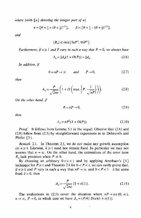
where (with [u] denoting the integer part of u)

f3 = [0 + ! - ( 0 + ~) 1/2 ],

and

Furthermore, if n ~ 1 and P vary in such a way that P -+ 0, we always have

(2.6)

In addition, if

O=nP-+ 00 and p-+o, (2.7)

then

d n = ~(1+0(max{p, fo}). (2.8)

On the other hand, if

O=nP-+O, (2.9)

then

(2.10)

Proof It follows from Lemma 5.1 in the sequel. Observe that (2.6) and (2.8) follow from (2.5) by straightforward expansions as in Deheuvels and Pfeifer [5].

Remark 2.1. In Theorem 2.1, we do not make any growth assumption on n ~ 1. Likewise, k ~ 1 need not remain fixed. In particular we may not assume that n -+ 00. On the other hand, the estimations of the error term Rn lack precision when P -A 0.

By choosing an arbitrary ° < B < 1 and by applying Arenbaev's [1] technique for P ~ B and Theorem 2.1 for 0< P < B, we can easily prove that, if n ~ 1 and P vary in such a way that nP -+ 00 and 0< P < 1 - b for some fixed b > 0, then

P An = ~ (1 + 0(1)).

y2ne (2.11 )

The evaluations in (2.5) cover the situation where nP -+ a E (0, 00),

n -+ 00, P -+ 0, in which case we have An = (P/4) D(a)(1 + 0(1 )).

4

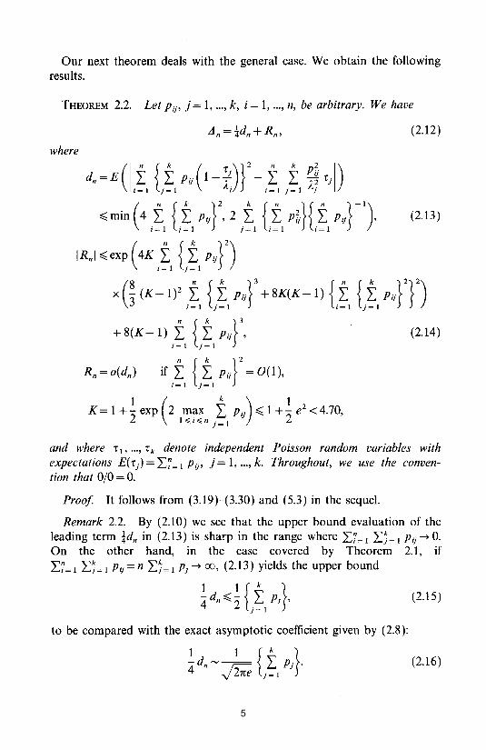
Our next theorem deals with the general case. We obtain the following results.

THEOREM 2.2. Let Pi}' j = 1, ... , k, i = 1, ... , n, be arbitrary. We have

(2.12)

where

(2.14 )

1 ( k) 1 K = 1 + -2 exp 2 m~x L P i} ~ 1 + -2 e2 < 4.70, 1~I~n j=1

and where T 1, .•. , T k denote independent Poisson random variables with expectations E( TJ = L:7= 1 Pi}' j = 1, ... , k. Throughout, we use the conven­tion that % = o.

Proof It follows from (3.19)-(3.30) and (5.3) in the sequel.

Remark 2.2. By (2.10) we see that the upper bound evaluation of the leading term !dn in (2.13) is sharp in the range where L:7= 1 L:J= 1 Pi} ~ o. On the other hand, in the case covered by Theorem 2.1, if L7= 1 LJ= 1 Pi} = n LJ= 1 Pj ~ 00, (2.13) yields the upper bound

1 1 {k } 4dn~2 .L Pj , J=l

(2.15)

to be compared with the exact asymptotic coefficient given by (2.8):

(2.16)

5

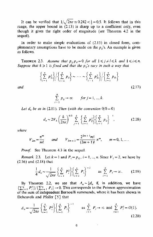
It can be verified that 1/~ ~ 0.242 < ~ = 0.5. It follows that in this range, the upper bound in (2.13) is sharp up to a coefficient only, even though it gives the right order of magnitude (see Theorem 4.2 in the sequel).

In order to make simple evaluations of (2.13) in closed form, com­plementary assumptions have to be made on the Pij's. An example is given as follows.

THEOREM 2.3. Assume that Pij Pi! = 0 for all 1 ~ j #1 ~ k and 1 ~ i ~ n. Suppose that k ~ 1 is fixed and that the P ij's vary in such a way that

and (2.17)

n

I Pij-+ 00 for j= 1, ... , k. i=1

Let dn be as in (2.11). Then (with the convention 010=0)

(2.18)

where

and m=0,1, ....

Proof See Theorem 4.3 in the sequel.

Remark 2.3. Let k = 1 and Pi = Pil, i = 1, ... , n. Since VI = 2, we have by (2.16) and (2.18) that

!d __ 1 {i p2}{ i p.}-1 4 n ~ i=1 I i=1 I

n

as I (2.19) i=1

By Theorem 2.2, we see that An - !dn if, in addition, we have {L7= 1 Pi} 1 {L7= 1 PJ -+ O. This corresponds to the Poisson approximation of the sum of independent Bernoulli summands, where it has been shown in Deheuve1s and Pfeifer [5] that

1 {n }{ n }-1 An=-- I P; I Pi ~ i=1 i=1

n n

as I Pi -+ 00 and I P; = O( 1). i= 1 i=1

(2.20)

6

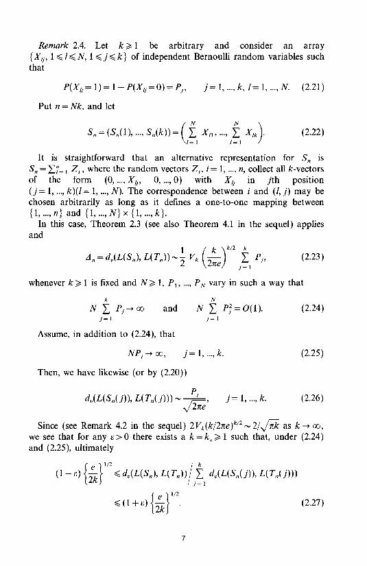
Remark 2.4. Let k;::: 1 be arbitrary and consider an array { X lj' 1 ~ 1 ~ N, 1 ~ j ~ k} of independent Bernoulli random variables such that

P(Xlj= 1)= I-P(Xlj=O)=Pj ,

Put n = Nk, and let

j= 1, ... , k, 1= 1, ... , N. (2.21)

It is straightforward that an alternative representation for Sn is Sn = :L7= 1 Z;, where the random vectors Z;, i = 1, ... , n, collect all k-vectors of the form (0, ... , X lj' 0, ... , 0) with X lj in jth position (j = 1, ... , k)(I = 1, ... , N). The correspondence between i and (I, j) may be chosen arbitrarily as long as it defines a one-to-one mapping between {I, ... , n} and {I, ... , N} x {I, ... , k}.

In this case, Theorem 2.3 (see also Theorem 4.1 in the sequel) applies and

(2.23)

whenever k;::: 1 is fixed and N;::: 1, PI' ... , P N vary in such a way that

k

N I Pj -+ 00 j=l

and

Assume, in addition to (2.24), that

N

N I P;=O(I). j=I

j= 1, ... , k.

Then, we have likewise (or by (2.20))

j= 1, ... , k.

(2.24 )

(2.25)

(2.26)

Since (see Remark 4.2 in the sequel) 2Vk(kI2ne)kI2 '" 21fo as k -+ 00,

we see that for any 8> 0 there exists a k = k e ;::: 1 such that, under (2.24) and (2.25), ultimately

{ e }I/2

~ (1 + 8) 2k . (2.27)

7

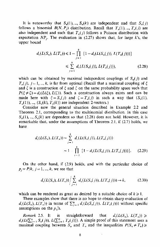
It is noteworthy that Sn(1), ... , Sn(k) are independent and that Sn(j) follows a binomial B(N, Pj) distribution. Recall that Tn(1), ... , Tn(j) are also independent and such that Tn( j) follows a Poisson distribution with expectation NPj • The evaluation in (2.27) shows that, for large k's, the upper bound

k

dv(L(Sn), L(Tn)) ~ 1 - n {I - dv(L(Sn(j)), L(Tn(j)))} j=l

k

~ I dv(L(Sn(j)), L(Tn(j))), (2.28) j=l

which can be obtained by maximal independent couplings of Sn(j) and Tn(j), j = 1, ... , k, is far from optimal (Recall that a maximal coupling of ~ and, is a construction of ~ and, on the same probability space such that P(~ =1= 0 = dv(L(~), L(O). Such a construction always exists and can be made here with ~ = Sn(j) and ,= Tn(j) in such a way that (Sn(1), Tn(1)), ... , (Sn(k), Tn(k)) are independent 2-vectors.)

Consider now the general situation described in Example 2.2 and Theorem 2.1, corresponding to the multinomial distribution. In this case Sn(1), ... , Sn(k) are dependent so that (2.28) does not hold. However, it is remarkable that, under the assumptions of Theorem 2.1, if (2.7) holds, we have

k

dv(L(Sn), L(Tn))- I dv(L(Sn(j)), L(Tn(j))) j= 1

k

-1 - n {1- dv(L(Sn(j)), L(Tn(j)))}. (2.29) j=l

On the other hand, if (2.9) holds, and with the particular choice of Pj = P/k, j = 1, ... , k, we see that

d,(L(Sn), L(Tn)) !it. d,(L(Sn(J)), L(Tn(J))) -> k, (2.30)

which can be rendered as great as desired by a suitable choice of k ~ 1. These examples show that there is no hope to obtain sharp evaluation of

dv(L(Sn), L(Tn)) in terms of LY= 1 dv(L(Sn(j)), L(Tn(j))) without specific assumptions on the Pij's.

Remark 2.5. It is straightforward that dv(L(Sn), L(Tn)) ~ dv(L(LY= 1 Sn(j)), L(LY= 1 Tn(j)))· A simple proof of this statement uses a maximal coupling between Sn and Tn and the inequalities P(Sn =1= Tn) ~

8

PC2:.J= 1 SnU) =I- LJ= 1 TnU)) ~ dv(L(LJ= 1 SnU)), L(LJ= 1 TnU)))· This enables one to obtain lower bounds for 11 n by using classical Poisson approximation arguments (see, e.g., Example 2.1).

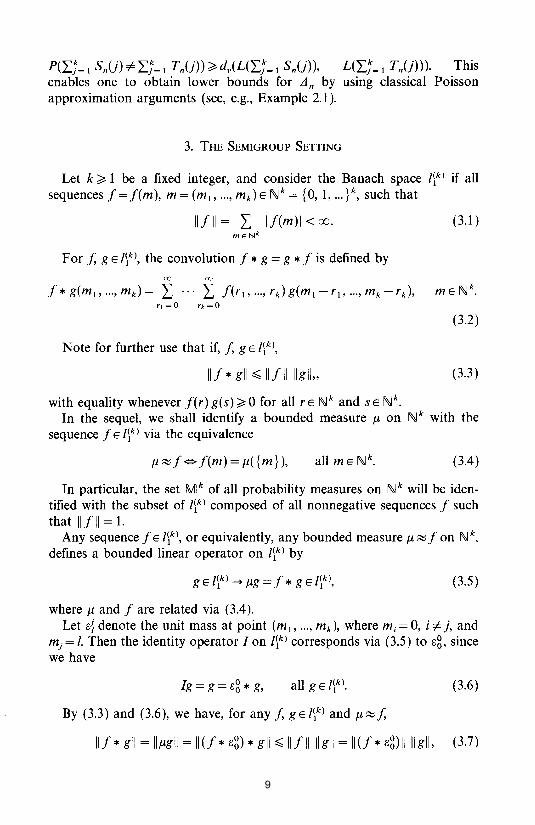
3. THE SEMI GROUP SETTING

Let k ~ 1 be a fixed integer, and consider the Banach space I~k) if all sequences 1= I(m), m = (ml, ... , mk) E Nk = {O, 1, ... }\ such that

11/11= L I/(m)l<oo. (3.1 ) mENk

For J, g E I~k), the convolution 1* g = g * I is defined by 00 00

l*g(m1,···,md= L ... L l(r1,···,rk)g(m1-r1,···,mk-rd, mEN k. rJ = 0 rk = 0

(3.2)

Note for further use that if, J, g E I~k),

III * gil ~ 11/11 IIgll" (3.3 )

with equality whenever l(r)g(s)~O for all rEN k and sENko In the sequel, we shall identify a bounded measure Ji on N k with the

sequence I E I~k) via the equivalence

Ji ~ I <=> I(m) = Ji( {m} ), (3.4 )

In particular, the set Mk of all probability measures on N k will be iden­tified with the subset of I~k) composed of all nonnegative sequences I such that II III = 1.

Any sequence I E I~k), or equivalently, any bounded measure Ji ~ I on N \ defines a bounded linear operator on I~k) by

(3.5)

where Ji and I are related via (3.4). Let e{ denote the unit mass at point (m 1, ... , md, where m i = 0, i =I- j, and

mj = I. Then the identity operator I on I~k) corresponds via (3.5) to eg, since we have

Ig=g=eg * g, (3.6)

By (3.3) and (3.6), we have, for any J, g E I~k) and Ji ~ J,

III * gil = IlJigli = 11(1 * eg) * gil ~ 11/11 II gil = 11(1 * e8)11l1gll, (3.7)

9

with equality when g = eg. This shows that the operator norm sup{ll/* gll/llgll: g#O} of the operator defined by (3.5) coincides with IIIII = III * egll. In the sequel, both norms will be denoted by 11/11.

Consider now, for j = 1, ... , k, the operator Bj defined by

(3.8)

It is straightforward that B}, ... , Bk commute and that the operator in (3.5) corresponds to

gE1ik)-+>I*g=( f··· f l(r}, ... ,rdB~l"'B~k)g. (3.9) q =0 rk=O

For j = 1, ... , k, A j = Bj - I defines the generator of the contraction semigroup {exp(ljAj), Ij ~ O}. The operator exp(ljAj) corresponds via (3.5) and (3.9) to a probability measure which is a product of unit masses at the origin for the coordinates 1, ... , j - 1, j + 1, ... , k, and of a Poisson distribution with mean Ij for the jth coordinate.

Likewise, the multiparameter semigroup

I}, ... , Ik ~ 0, (3.10)

corresponds to products of probability measures having mean I j on the jth coordinate, j = 1, ... , k.

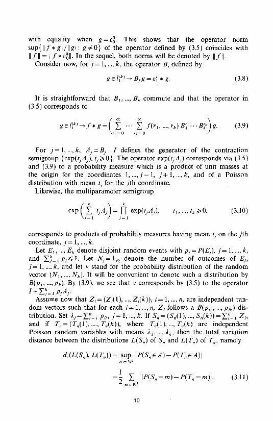
Let E}, ... , Ek denote disjoint random events with Pj = P(Ej ), j = 1, ... , k, and LY=} Pj ~ 1. Let Nj = 1 Ej denote the number of outcomes of Ej , j = 1, ... , k, and let v stand for the probability distribution of the random vector (N}, ... , N k ). It will be convenient to denote such a distribution by B(p}, ... , pd· By (3.9), we see that v corresponds by (3.5) to the operator 1+ LY=} pjAj'

Assume now that Zi= (Zi(I), ... , Zi(k)), i= 1, ... , n, are independent ran-dom vectors such that for each i = 1, ... , n, Zi follows a B(Pi}, ... , Pik) dis­tribution. Set Aj = L7=} Pi}' j = 1, ... , k. If Sn = (Sn(1), ... , Sn(k)) = L7= 1 Zj, and if Tn=(Tn(1)' .... ,Tn(k)), where Tn(1), ... ,Tn(k) are independent Poisson random variables with means )'}' ... , Ak , then the total variation distance between the distributions L(Sn) of Sn and L(Tn) of Tn, namely

dv(L(Sn), L(Tn)) = sup IP(Sn E A) - P(Tn E A)I AcNk

10

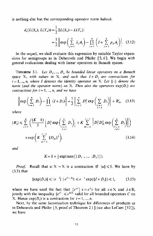
is nothing else but the corresponding operator norm halved:

In the sequel, we shall evaluate this expression by suitable Taylor expan­sions for semigroups as in Deheuvels and Pfeifer [5, 6]. We begin with general evaluations dealing with linear operators in Banach spaces.

THEOREM 3.1. Let Db ... , Dn be bounded linear operators on a Banach space X, with values in X, and such that I + D i are contractions for i = 1, ... , n, where I denotes the identity operator on X. Let II ·11 denote the norm (and the operator norm) on X. Then also the operators exp(DJ are contractions for i = 1, ... , n, and we have

1= I

where

(3.14 )

and

K = 1 +! exp(max {IIDIII, ... , liDnll}).

Proof Recall that u: X -+ X is a contraction iff Ilull ~ 1. We have by (3.3) that

(3.15 )

where we have used the fact that {eM} x = e)'x for all x E X and It E IR, jointly with the inequality Ileell ~ e ilCil valid for all bounded operators C on X. Hence exp(DJ is a contraction for i = 1, ... , n.

Next, by the same factorization technique for differences of products as in Deheuvels and Pfeifer [5, proof of Theorem 2.1] (see also LeCam [12]), we have

11

I¥- i

I¥- i

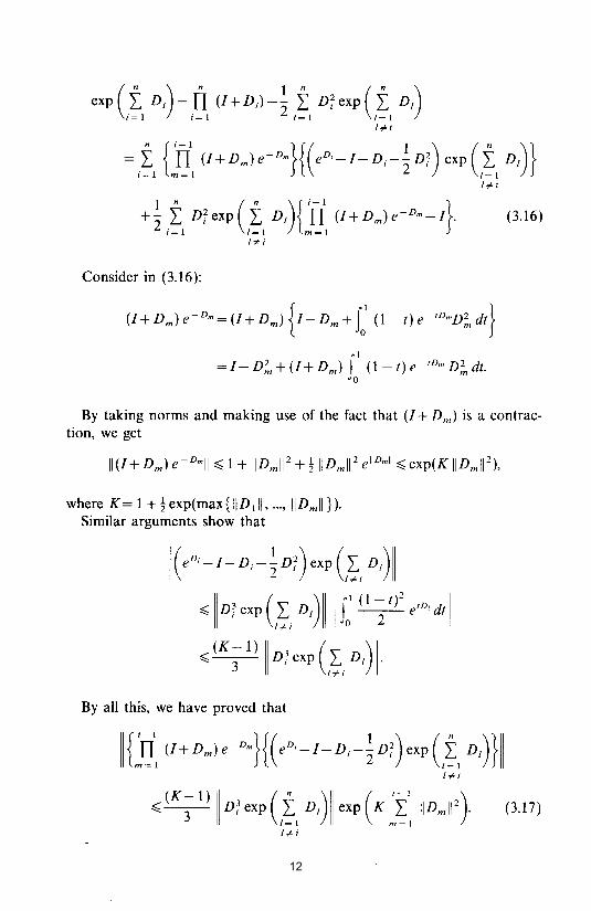
+~ it! Dfexp Ct! DI)U( (I+Dml e-Dm_/}. (3.16)

I¥- i

Consider in (3.16):

(I + Dml e- Dm ~ (1+ Dml {I - Dm + J: (1- Il e-'DmD~ dl}

= I - D~ + (I + Dm) ( (1- t) e- tDm D~ dt.

By taking norms and making use of the fact that (I + D m) is a contrac­tion, we get

where K = 1 +! exp(max {IIDIII, ... , IIDmll}). Similar arguments show that

II(eD;-I-Di-~ Df) exp C~i DI)II

" liD; exp C~i DI)IIII J: (1 ~ Il' e'Di dl II

,,(K; 1) II D; exp C~i DI)II

By all this, we have proved that

I¥- i

(3.17)

12

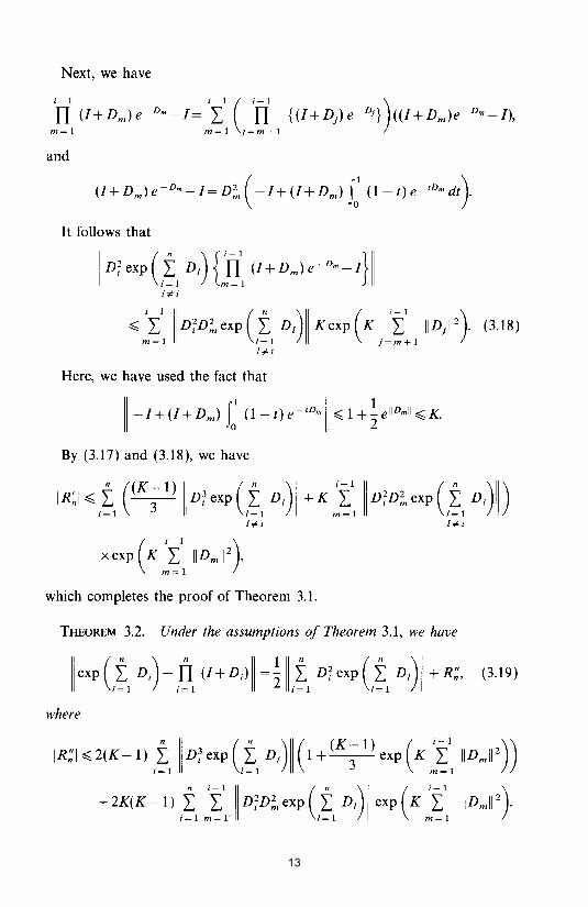
Next, we have

and

It follows that

,., I II D~D;' exp Ct DJ)II K exp ( K iJ: I IID;112). (3.18)

l-=/=i

Here, we have used the fact that

11-1+ (1+ Dm) f: (1- t) e-<Om II'" 1+ ~ ellDml1 ,., K.

By (3.17) and (3.18), we have

which completes the proof of Theorem 3.1.

THEOREM 3.2. Under the assumptions of Theorem 3.1, we have

where

IR:I ,.,2(K-l) t liD; exp (t DI)II (1 + (K; 1) exp (K I IIDmIl2))

+2K(K-l) itl I II D~D;' exp Ctl DI)II exp (K I II Dm 112).

13

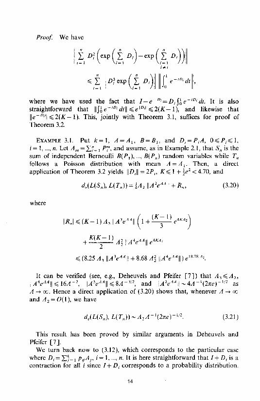
Proof We have

ttl D; (exp (t DI) - exp (t D) )11 l#i

~itl liD; exp (t D1)1111( e-midlll,

where we have used the fact that 1- e- Di = Dd6 e- tDj dt. It is also straightforward that IIH e- tDi dtll ~ e liDili ~ 2(K - 1), and likewise that lie-Dill ~ 2(K -1). This, jointly with Theorem 3.1, suffices for proof of Theorem 3.2.

EXAMPLE 3.1. Put k= 1, A =Al' B=B1 , and Di=PiA, O~Pi~ 1, i = 1, ... , n. Let Am = 'L7= 1 P7\ and assume, as in Example 2.1, that Sn is the sum of independent Bernoulli B(Pd, ... , B(Pn) random variables while Tn follows a Poisson distribution with mean A = AI' Then, a direct application of Theorem 3.2 yields IIDil1 = 2P i , K ~ 1 + !e2 < 4.70, and

where

IRnl ~ (K -1) A311A3eAAII (1 + (K; 1) e4KA')

+ K(K2- 1) A~ IIA4eAA II e4KA2

~ (8.25 A3 IIA3eAAII + 8.68 A~ IIA4eAAII) e18.78 A2.

(3.20)

It can be verified (see, e.g., Deheuvels and Pfeifer [7]) that A 3 ~ A 2,

IIA4eAA II ~ 16A -2, IIA3eAA II ~ 8A -3/2, and IIA 2eAA 11- 4A -1(2ne )-1/2 as A ~ 00. Hence a direct application of (3.20) shows that, whenever A ~ 00

and A2 = 0(1), we have

(3.21 )

This result has been proved by similar arguments m Deheuvels and Pfeifer [7].

We turn back now to (3.12), which corresponds to the particular case where Di = 'LY= 1 pijA}, i = 1, ... , n. It is here straightforward that 1+ Di is a contraction for all i since 1+ D i corresponds to a probability distribution.

14

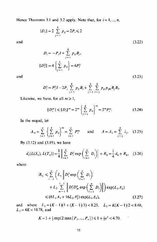
Hence Theorems 3.1 and 3.2 apply. Note that, for i = 1, ... , n,

k

IIDil1 =2 L Pij=2Pi~2 j=l

and (3.22)

k

Di= -PJ+ L PijBj' j=l

and (3.23 )

k k k

Df=PfI-2Pi L pijBj + L L PijPijkBjB1•

j=l j=I/=1

Likewise, we have, for all m ;::: 1,

IIDrll ~ IIDili m = 2m {.f pij}m = 2mPt J=1

(3.24 )

In the sequel, let

k

and A = Al = L Aj . (3.25) j=1

By (3.12) and (3.19), we have

d,(L(S.), L(T.» ~{ II i~1 D; exp (,~I DI)II + R. ~{d. + R., (3.26)

where

IRnl" t ( Ll II D; exp (,~1 DI)II

+ L2 I II D;D~ exp (,~1 DI)II) exp(L,A2)

~ (8LI A 3 + 16L2A~) exp(L 3 A 2), (3.27)

and where Ll = (K -1)(1 + (K - 1 )/3) < 8.25, L2 = K(K -1 )/2 < 8.68, L3 = 4K < 18.78, and

K = 1 + ! exp(2 max { PI' ... , P n} ) ~ 1 + !e2 < 4.70.

15

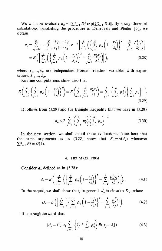
We will now evaluate dn = 11L:7= 1 Df exp(L:I= 1 D/)II. By straightforward calculations, paralleling the procedure in Deheuvels and Pfeifer [5], we obtain

q=O

00 )/, ••• Ark 1 n ({ k ( )}2 k 2)1 " 1 k -A" " 1 _!.i. _ " pi;rj ~ ,..., e ~ ~ Plj A ~ A2

rk = 0 r 1 . r k • i = 1 i = 1 ) i = 1 )

=E(I.f ({.f Pij (1- i.)}2 - .f pi;i)I), 1=1 )=1 ) J=1 J

(3.28)

where T 1, .•. , T k are independent Poisson random variables with expec­tations AI, ... , Ak'

Routine computations show also that

( n {k ( T.)}2) (n k P~.T') k {n }{ n }-1 E.L .LPij l-i =E.L.L 1/ =.L .LP~ .LPij . 1=1 J=1 ) 1=IJ=1 J J=1 1=1 1=1

(3.29)

It follows from (3.29) and the triangle inequality that we have in (3.28)

(3.30)

In the next section, we shall detail these evaluations. Note here that the same arguments as in (3.22) show that Rn = o(dn) whenever

L:7 = 1 Pf = O( 1 ).

4. THE MAIN TERM

Consider dn defined as in (3.28):

(I n ({ k ( T.)}2 k p~.T·)I) dn=E.L .L Pi;' l-i -.L 1/ .

1=1 J=1 J J=1 J

(4.1 )

In the sequel, we shall show that, in general, dn is close to D n , where

Dn = E (I.f ({.f Pij (l-r)}2 -.f ~~)I)· (4.2) 1=1 J=1 ) J=I)

It is straightforward that

(4.3 )

16

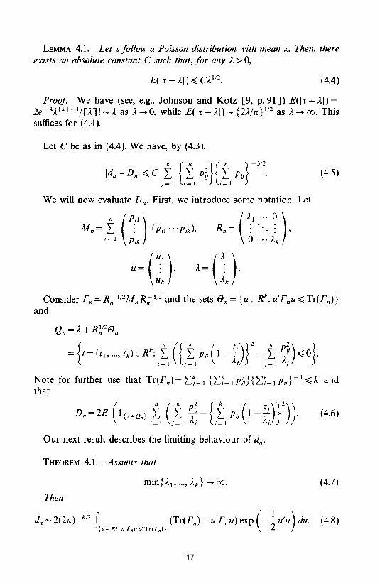
LEMMA 4.1. Let 7: follow a Poisson distribution with mean A. Then, there exists an absolute constant C such that, for any A> 0,

(4.4 )

Proof We have (see, e.g., Johnson and Kotz [9, p. 91]) E(I7:-AI)= 2e- AA[A] + I/[A]! "" A as A -+ 0, while E(I7: - AI) "" {2Aln} 1/2 as A -+ 00. This suffices for (4.4).

Let C be as in (4.4). We have, by (4.3),

(4.5)

We will now evaluate Dn- First, we introduce some notation. Let

Consider Fn = R;; 1/2MnR;; 1/2 and the sets en= {UERk: u'Fnu~Tr(Fn)} and

{ n ({ k ( t .)} 2 k P~') } = t= (tl' ... , tdERk: .L .L Pi} l-i -.L / ~o .

1=1 )=1 ) )=1)

Note for further use that Tr(Fn)=L:;=1 {L:7=IPt}{L:7=IPi}}-I~k and that

( n ( k P~' {k ( 7: .)}2)) Dn=2E 1{-ce Qn }.L .L /- .L Pi} I-t .

1=1 )=1) )=1 )

(4.6)

Our next result describes the limiting behaviour of dn •

THEOREM 4.1. Assume that

(4.7)

Then

dn"" 2(2n)-k/2 f (Tr(Fn) - u' Fnu) exp (- -21

u'u) duo (4.8) {u e Rk: u'TnU";; Tr(Tn)}

17

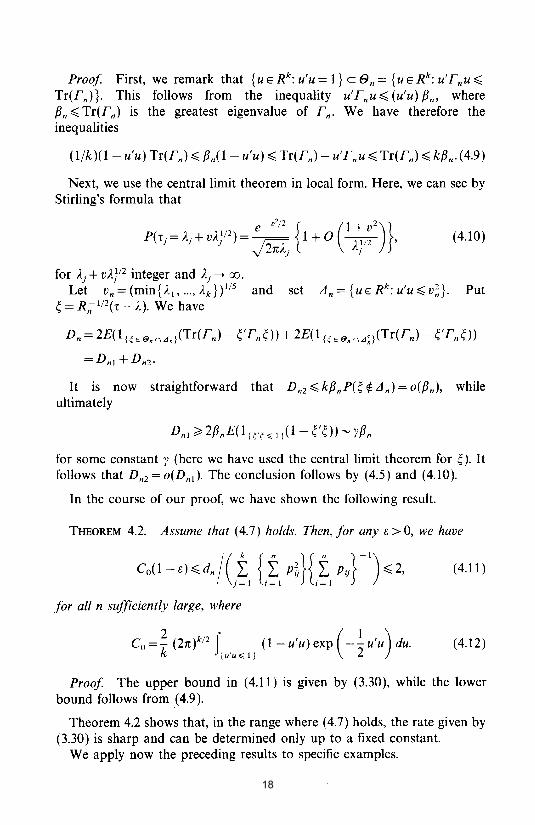
Proof First, we remark that {uERk:u'u=l}cen={uERk:u'rnu~ Tr(rn)}. This follows from the inequality u'rnu~ (u'u) f3n, where f3n ~ Tr(rn) is the greatest eigenvalue of rn. We have therefore the inequalities

Next, we use the central limit theorem in local form. Here, we can see by Stirling's formula that

P(rj = Aj + VAJl2) = j-"'I: {I + 0 (1 ;/~2)}, (4.10) 2nAj }

for Aj + vAJl2 integer and Aj ---+ 00.

Let vn =(min{21, ... ,2d)1/5 and set An={UERk:u'u~v~}. Put ~ = R;1/2(r - 2). We have

Dn = 2E(1 U; E ennAn}(Tr(rn) -~' rn~» + 2E(1 {~E ennA~}(Tr(rn) - ~'rn~»

=Dn1 +Dn2 ·

It is now straightforward that Dn2~kf3nP(~~An)=o(f3n)' while ultimately

for some constant y (here we have used the central limit theorem for ~). It follows that Dn2 = o(Dnd. The conclusion follows by (4.5) and (4.10).

In the course of our proof, we have shown the following result.

THEOREM 4.2. Assume that (4.7) holds. Then, for any B > 0, we have

for all n sufficiently large, where

Co = -k2

(2n)k/2 f, (1- u'u) exp (--21

u'u) duo (4.12) {u u:O;; 1}

Proof The upper bound in (4.11) is given by (3.30), while the lower bound follows from (4.9).

Theorem 4.2 shows that, in the range where (4.7) holds, the rate given by (3.30) is sharp and can be determined only up to a fixed constant.

We apply now the preceding results to specific examples.

18

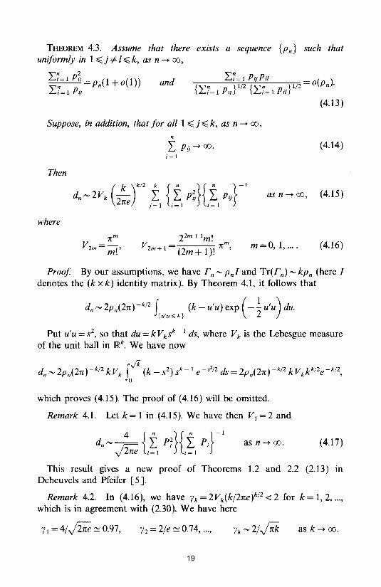
THEOREM 4.3. Assume that there exists a sequence {Pn} such that uniformly in 1 ~ j =1= I ~ k, as n -+ 00,

and L:7=1 PijPil ( )

{ "~ .. } 1/2 {"~ . } 1/2 = 0 Pn . L....1=IPIj L....1=IPil

(4.13 )

Suppose, in addition, that for all 1 ~ j ~ k, as n -+ 00,

n

I Pij-+ 00. (4.14 ) i=l

Then

as n -+ 00, (4.15)

where

m=0,1, .... (4.16)

Proof By our assumptions, we have rn '" PnI and Tr(rn) '" kPn (here I denotes the (k x k) identity matrix). By Theorem 4.1, it follows that

dn '" 2Pn(2n) -k/2 f (k - u'u) exp (-! u'u) duo {u'u';;;k} 2

Put U'U=S2, so that du=kVksk- 1 ds, where Vk is the Lebesgue measure of the unit ball in ~k. We have now

which proves (4.15). The proof of (4.16) will be omitted.

Remark 4.1. Let k = 1 in (4.15). We have then VI = 2 and

4 {n }{ n }-1 dn ",-- I Pi I Pi foe i=1 i=l

as n -+ 00. (4.17)

This result gives a new proof of Theorems 1.2 and 2.2 (2.13) in Deheuvels and Pfeifer [5].

Remark 4.2. In (4.16), we have Yk=2Vk(kI2ne)k/2<2 for k= 1, 2, ... , which is in agreement with (2.30). We have here

Yl = 41foe ~ 0.97, Y2 = 21e ~ 0.74, ... , as k -+ 00.

19

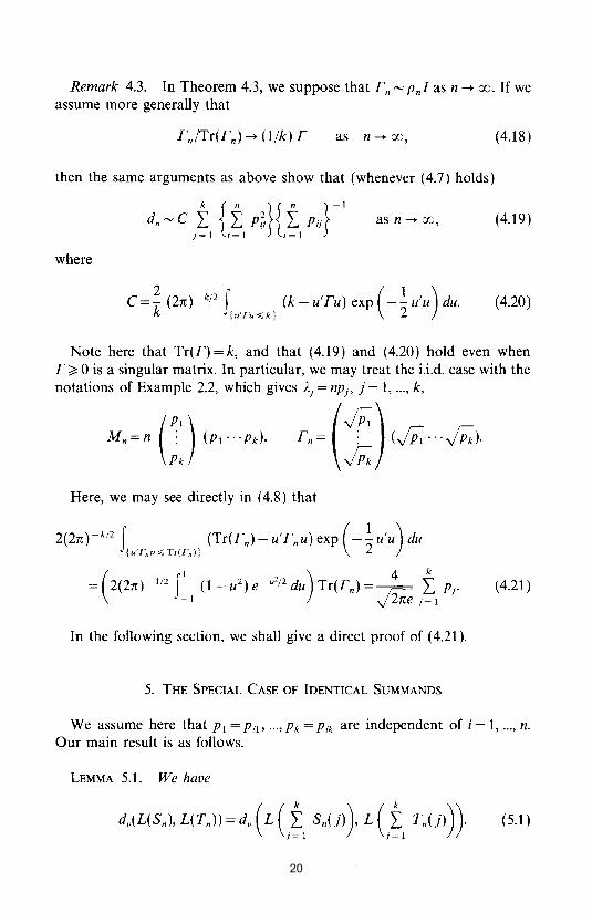
Remark 4.3. In Theorem 4.3, we suppose that rn '" PnI as n --+ 00. If we assume more generally that

as n --+ 00, ( 4.18)

then the same arguments as above show that (whenever (4.7) holds)

as n --+ 00, ( 4.19)

where

C =-k2

(2n)-k/2 f (k - u'ru) exp (-~ u'u) duo (4.20) {uTu~k} 2

Note here that Tr(r) = k, and that (4.19) and (4.20) hold even when r~ 0 is a singular matrix. In particular, we may treat the i.i.d. case with the notations of Example 2.2, which gives )'j = npj' j = 1, ... , k,

(fi:) c ~ rn= : ("';PI ···Jpd. vP:

Here, we may see directly in (4.8) that

(4.21 )

In the following section, we shall give a direct proof of (4.21).

5. THE SPECIAL CASE OF IDENTICAL SUMMANDS

We assume here that PI = Pil, ... , Pk = Pik are independent of i = 1, ... , n. Our main result is as follows.

LEMMA 5.1. We have

20

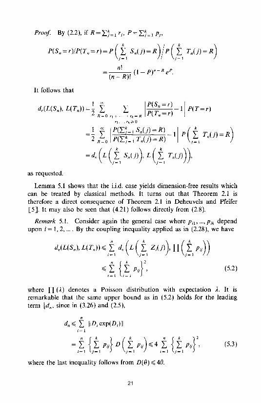
n! n-R P (n-R)! (l-P) e.

It follows that

as requested.

Lemma 5.1 shows that the i.i.d. case yields dimension-free results which can be treated by classical methods. It turns out that Theorem 2.1 is therefore a direct consequence of Theorem 2.1 in Deheuvels and Pfeifer [5J. It may also be seen that (4.21) follows directly from (2.8).

Remark 5.1. Consider again the general case where Pi!, ... , Pik depend upon i = 1,2, .... By the coupling inequality applied as in (2.28), we have

(5.2)

where n (A) denotes a Poisson distribution with expectation A. It is remarkable that the same upper bound as in (5.2) holds for the leading term ~dn' since in (3.26) and (2.5),

n

dn ::::; L IIDiexp(DJII i= 1

n {k } (k \ n {k }2 =.L .L Pij D .L pij)::::;4.L .L Pij , 1=1 J=l J=l 1=1 J=l

(5.3 )

where the last inequality follows from D( 8) ::::; 48.

21

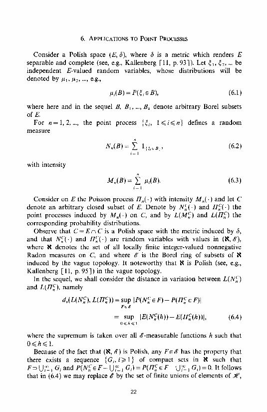
6. ApPLICATIONS TO POINT PROCESSES

Consider a Polish space (E, b), where b is a metric which renders E separable and complete (see, e.g., Kallenberg [11, p. 93]). Let ~1' ~2'''' be independent E-valued random variables, whose distributions will be denoted by /11, /12' ... , e.g.,

(6.1 )

where here and in the sequel B, B 1 , ... , Bk denote arbitrary Borel subsets of E.

For n = 1, 2, ... , the point process {~i' 1 ~ i ~ n} defines a random measure

n

Nn(B) = I 1{~iEB}' (6.2) i=l

with intensity n

Mn(B) = I lli(B). (6.3 ) i=l

Consider on E the Poisson process JIn ( .) with intensity M n (·) and let C denote an arbitrary closed subset of E. Denote by N;(·) and JI;(.) the point processes induced by Mn{-) on C, and by L(M;) and L(JI;) the corresponding probability distributions.

Observe that C = En C is a Polish space with the metric induced by b, and that N;(·) and JI;(.) are random variables with values in (N, <ff), where N denotes the set of all locally finite integer-valued nonnegative Radon measures on C, and where <ff is the Borel ring of subsets of N induced by the vague topology. It noteworthy that N is Polish (see, e.g., Kallenberg [11, p. 95]) in the vague topology.

In the sequel, we shall consider the distance in variation between L(N;) and L(JI;), namely

dv(L(N;), L(JI;)) = sup IP(N; E F) - P(JI; E F)I

= sup IE(N;(h))-E(JI;(h))I, (6.4) O,;;;h,;;;l

where the supremum is taken over all <ff -measurable functions h such that O~h~1.

Because of the fact that (N, <ff) is Polish, any FE <ff has the property that there exists a sequence {G i' i ~ 1} of compact sets in N such that F~ ur: 1 Gj and P(N; E F - ur: 1 GJ = P(JI; E F - ur: 1 GJ = O. It follows that in (6.4) we may replace <ff by the set of finite unions of elements of Yf,

22

where Yf is a basis for the vague topology (by this, we mean that, for any v E N and for any neighborhood V of v, there exists a neighborhood W of v such that We V and WE Yf).

We shall consider the case where Yf collects all sets of the form {mEN:m(BJ=ni' i=l, ... ,k}, where B1, ... ,Bk are Borel subsets of E, k?:- 1, and nb ... , nk are nonnegative integers. Recall that Vn --+ v vaguely iff for any B such that v(oB) = 0, we have vn(B) --+ v(B), which implies vn(B) = v(B) for n large enough. We have evidently

dv(L(N;/), L(Il;))

= sup IP(N; E F) - P(Il; E F)I

= sup sup dv(L{ N;(Bd, ... , N;(Bk )}, L{ Il;(Bd, ... , Il;(Bk )}). (6.5) k;. 1 B\, ... , Bk

Here we can assume, without loss of generality, that B 1 , ... , Bk are disjoint Borel subsets of E.

By (6.5), the evaluation of dv(L(N;), L(Il;)) can be reduced to the problem treated in the preceding section. As a direct application, we obtain:

THEOREM 6.1. Assume that j.l = j.li is independent of i = 1, 2, ... , n. Let P = j.l( C) and () = nP. Then

d"(L(N;), L(O;» =~ PO (0"-1~~ - 0) OH~ - 0») e -6 + Rn, (6.6)

where ex and f3 and Rn are as in Theorem 2.1. In addition, if n, j.l, and C vary in such a way that, for a fixed 8 > 0,

nj.l( C) --+ 00 and j.l(C) < 1- 8, (6.7)

then

(6.8)

On the other hand, if

(6.9)

then

(6.10)

Proof By (6.5) and Theorem 2.1, we have dv = sup(!dn + R n), where the supremum is taken over all B 1, ... , B k disjoint Borel subsets of C. It suffices

23

now to use the fact that idn and IRnl are increasing functions of Il(U~= 1 BJ, and maximal when U~= 1 Bi = C. The conclusion follows by (2.11 ).

In order to obtain similar evaluations in the non-i.i.d. case, assume that there exists a Radon measure v on E such that Ili ~ v for i = 1, ... , n. Such a measure always exists, since we way take v = L:7= 1 Ili'

Let Ii = dill dv denote the Radon-Nikodym derivative of Ili respectively to v, and consider the Radon measure (J n defined (with the convention 010=0) by

(6.11)

Observe that (J n is independent of v. Furthermore, since the choice v = L:7= 1 Ili implies Ii ~ 1 (v-a.e.), we have evidently (J n ~ L:7= 1 Ili' Note also that, whenever Il 1 = ... = Iln = Il, we have (J n = Il·

Let us now use again Theorem 2.2 and (6.5). It is straightforward that if we use the upper bound (3.30) for dn , we obtain the upper bound

We obtain therefore the following result.

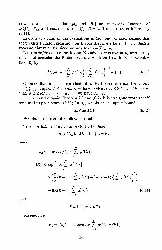
THEOREM 6.2. Le t (J n be as in (6.11). We have

dv(L(N~), L(II~)) = !dn + R n,

where n

dn ~ min(2(J n( C), 4 I 1l7( C)), i=l

IRnl';; exp ( 4K ;tl 1';( c»)

x G (K ~ I)' ;tl I';(C) + 8K(K ~ 1) ttl I':(C) n n

+8K(K-1) I lli(C)~ i=l

and

Furthermore, n

whenever I 1l7( C) = O( 1). i= 1

(6.12)

(6.13)

24

Remark 6.1. The condition 1:7 = 1 J17( C) = O( 1) is probably not necessary for the validity of (6.13) (see, e.g., Theorem 6.1).

ACKNOWLEDGMENTS

We thank the referee for some helpful comments and remarks. The second author is indeb­ted to the Deutsche Forschnungsgemeinschaft for financial support by a Heisenberg research grant.

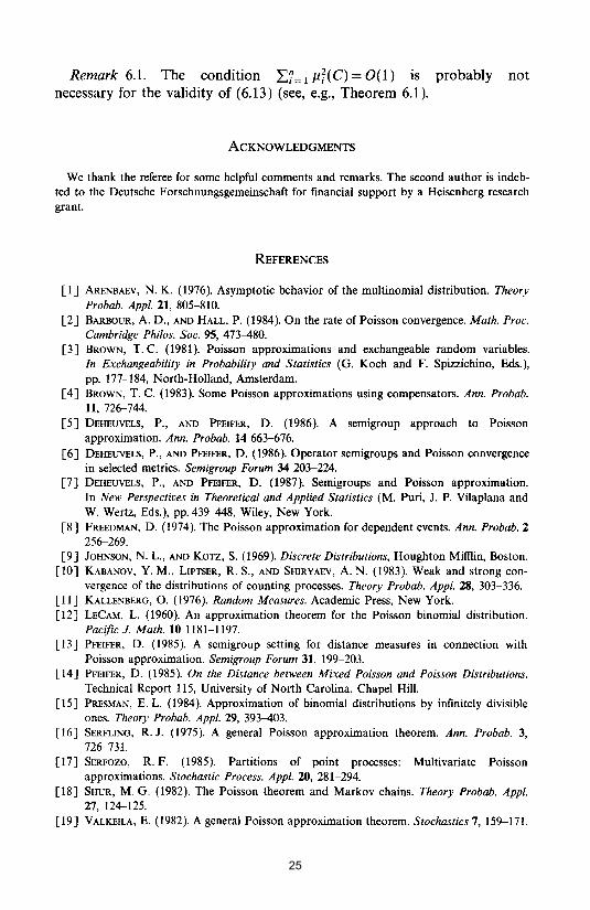
REFERENCES

[1] ARENBAEV, N. K. (1976). Asymptotic behavior of the multinomial distribution. Theory Probab. Appl. 21, 805-810.

[2] BARBOUR, A. D., AND HALL, P. (1984). On the rate of Poisson convergence. Math. Proc. Cambridge Phi/os. Soc. 95, 473-480.

[3] BROWN, T. C. (1981). Poisson approximations and exchangeable random variables. In Exchangeability in Probability and Statistics (G. Koch and F. Spizzichino, Eds.), pp. 177-184, North-Holland, Amsterdam.

[4] BROWN, T. C. (1983). Some Poisson approximations using compensators. Ann. Probab. 11, 726--744.

[5] DEHEUVELS, P., AND PFEIFER, D. (1986). A semigroup approach to Poisson approximation. Ann. Probab. 14663--676.

[6] DEHEUVELS, P., AND PFEIFER, D. (1986). Operator semigroups and Poisson convergence in selected metrics. Semigroup Forum 34 203-224.

[7] DEHEUVELS, P., AND PFEIFER, D. (1987). Semigroups and Poisson approximation. In New Perspectives in Theoretical and Applied Statistics (M. Puri, 1. P. Vilaplana and W. Wertz, Eds.), pp.439-448, Wiley, New York.

[8] FREEDMAN, D. (1974). The Poisson approximation for dependent events. Ann. Probab. 2 256--269.

[9] JOHNSON, N. L., AND KOTZ, S. (1969). Discrete Distributions, Houghton Miffiin, Boston. [10] KABANOV, Y. M., LIPTSER, R. S., AND SHIRYAEV, A. N. (1983). Weak and strong con­

vergence of the distributions of counting processes. Theory Probab. Appl. 28, 303-336. [11] KALLENBERG, O. (1976). Random Measures. Academic Press, New York. [12] LECAM, L. (1960). An approximation theorem for the Poisson binomial distribution.

Pacific J. Math. 10 1181-1197. [13] PFEIFER, D. (1985). A semigroup setting for distance measures in connection with

Poisson approximation. Semigroup Forum 31, 199-203. [14] PFEIFER, D. (1985). On the Distance between Mixed Poisson and Poisson Distributions.

Technical Report 115, University of North Carolina, Chapel Hill. [15] PRESMAN, E. L. (1984). Approximation of binomial distributions by infinitely divisible

ones. Theory Probab. Appl. 29, 393-403. [16] SERFLING, R. J. (1975). A general Poisson approximation theorem. Ann. Probab. 3,

726--731. [17] SERFOZO, R. F. (1985). Partitions of point processes: Multivariate Poisson

approximations. Stochastic Process. Appl. 20, 281-294. [18] SHUR, M. G. (1982). The Poisson theorem and Markov chains. Theory Probab. Appl.

27, 124-125. [19] VALKEILA, E. (1982). A general Poisson approximation theorem. Stochastics 7,159-171.

25