RI 9352 REPORT OF INVESTIGATIONS/1991

PLEASE DO NaT REMOVE FR(jVI LIBRARY

Rotational Failure Mechanisms Using Multiple Friction Circles for Stability Analysis

By Douglas A. Crum

UNITED STATES DEPARTMENT OF THE INTERIOR

BUREAU OF MINES

------~--

tiC Pnr('~'l of Mines ""1

~. .~ :: .;~ ~ r:~h Center

I

Mission: As the Nation's principal conservation agency, the Department of the Interior has respon­sibility for most of our nationally-owned public lands and natural and cultural resources. This includes fostering wise use of our land and water resources, protecting our fish and wildlife, pre­serving the environmental and cultural values of our national parks and historical places, and pro­viding for the enjoyment of life through outdoor recreation. The Department assesses our energy and mineral resources and works to assure that their development is in the best interests of all our people. The Department also promotes the goals of the Take Pride in America campaign by encouraging stewardship and citizen responsibil­ity for the public lands and promoting citizen par­ticipation in their care. The Department also has a major responsibility for American Indian reser­vation communities and for people who live in Island Territories under U.S. Administration.

......

Report of Investigations 9352

RotatiC?nal Failure Mechanisms Using Multiple Friction Circles for Stability Analysis

By Douglas A. Crum

UNITED STATES DEPARTMENT OF THE INTERIOR Manuel Lujan, Jr., Secretary

BUREAU OF MINES T S Ary, Director

Library of Congress Cataloging in Publication Data:

Crum, Douglas A. Rotational failure mechanisms using multiple friction circles for stability

analysis / by Douglas A. Crum.

p. em. - (Report of investigations; 9352)

Includes bibliographical references (p. 21).

1. Spoil banks-Mathematical models. 2. Slopes (Soil mechanics)-Mathematical models. 3. Eccentric loads-Mathematical models. I. Title. II. Series: Report of investigations (United States. Bureau of Mines); 9352.

TN23.U43 [TN292] 622 s-dc20 [624.1'5] 90-2313 elP

I I

CONTENTS Page

Abstract. . . . . . . . . . . . . . . . . . . . . . . . . . . . . . . . . . . . . . . . . . . . . . . . . . . . . . . . . . . . . . . . . . . . . . . . . . . 1 Introduction . . . . . . . . . . . . . . . . . . . . . . . . . • . . . . . . . . . . . . . . . . . . . . . . . . . . . . . . . . . . . . . . . . . . . . . . 2 Disclaimer of liability ................................................................. 4 General method and derivation of equations ................................................ 4

Resultant cohesive force . . . . . . . . . . . . . . . . . . . . . . . . . . . . . . . . . . . . . . . . . . . . . . . . . . . . . . . . . . . . . 4 Resultant friction force . . . . . . . . . . . . . . . . . . . . . . . . . . . . . . . . . . . . . . . . . . . . . . . . . . . . . . . . . . . . . . 5 Resolution of forces ....................•........................................... 6 Kinematics . . . . . . . . . . . . . . . . . . . . . . . . . . . . . . . . . . . . . . . . . . . . . . . . . . . . . . . . . . . . . . . . . . . . . . . 7 Factors of safety . . . . . . . . . . . . . . . . . . . . . . . . . . . . . . . . . . . . . . . . . . . . . . . . . . . . . . . . . . . . . . . . . . . 10

Friction ....................................................................... 10 Cohesion . . . . . . . . . . . . . . . . . . . . . . . . . . . . . . . . . . . . . . . . . . . . . . . . . . . . . . . . . . . . . . . . . . . . . . 11 Multisurface mechanisms .......................................................... 11

Optimization ..................................................................... 11 Eccentric loads. . . . . . . . . . . . . . . . . . . . . . . . . . . . . . . . . . . . . . . . . . . . . . . . . . . . . . . . . . . . . . . . . . . . . . 14

Single-circle mechanism without uplift ................. " ...... ". . . . . . .. . . . . . . . . . . . . . . . . . . . . 14 Single-circle mechanism with uplift ..................................................... 14 Three-circle mechanism ............................................................. 15

Effect of embedment ................................................................. 17 Bearing capacity calculations near slopes . . . . . . . . . . . . . . . . . . . . . . . . . . . . . . . . . . . . . . . . . . . . . . . . . . . 18 Conclusions ..................................................... :.................. 20 References . . . . . . . . . . . . . . . . . . . . . . . . . . . . . . . . . . . . . . . . . . . . . . . . . . . . . . . . . . . . . . . . . . . . . . . . . 21 Bibliography . . . . . . . . . . . . . . . . . . . . . . . . . . . . . . . . . . . . . . . . . . . . . . . . . . . . . . . . . . . . . . . . . . . . . . . . 21 Appendix A.-Notation . . . . . . . . . . . . . . . . . . . . . . . . . . . . . . . . . . . . . . . . . . . . . . . . . . . . . . . . . . . . . . . . 22 Appendix B.-Glossary ................................................................ 23 Appendix C.-oPTIC code listing ........................................................ 24

ILLUSTRATIONS

1. Circular failure surface in friction circle method ......................................... . 2. Three-circle mechanism for foundation collapse ......................................... . 3. Five-circle mechanism for active retaining wall ........................,....... ~ . . . . . . . . . . 4. Resultant cohesive force along circular arc .. . . . . . . . . . . . . . . . . . . . . . . . . . . . . . . . . . . . . .. . . . . . . 5. Resultant friction force on circular arc ................................................ . 6. General system of forces on two-wedge mechanism ...................................... . 7. Force polygon for two-wedge mechanism .............................................. . 8. Rotating wedges ................................................................ . 9. Hodographs of rotating wedges ..................................................... .

10. Construction of hodograph for mechanism composed of three friction circles .................... . 11. Shearing resistances .............................................................. . 12. Flowchart for Hooke and Jeeves method .............................................. . 13. Flowchart for optimization procedure in code OPTIC ..................................... . 14. Equivalent footings .............................................................. . 15. Single-circle mechanism without uplift ................................................ . 16. Single-circle mechanism with uplift . . . . . . . . . . . . . . . . . . . . . . . . . . . . . . . . . . . . . . . . . . . . . . . . . . . . 17. Effect of eccentricity on bearing capacity .............................................. . 18. Failure mechanisms of strip footings .................................................. . 19. Assumed mechanism for bearing capacity factors ........................................ . 20. Analysis of embedded footing with bearing capacity factors ................................. .

2 3 3 5 5 7 8 8 9 9

10 12 13 15 15 15 16 16 17 18

~·i

ii

ILLUSTRATIONS-Continued Page

21. Kinematic rigid-block mechanism .................................................... 19 22. Comparison of bearing capacity factors by two-wedge rigid-block method and two-wedge friction circle

method .................................................................. ,'... 19 23. Collapse mechanism for embedded foundation with eccentric load near slope . . . . . . . . . . . . . . . . . . . . 20

C-1. Values for input parameter to choose mechanism in code OPTIC ............................ 24

TABLE

1. Partial listing of bearing capacity factors. . . . . . . . . . . . . . . . . . . . . . . . . . . . . . . . . . . . . . . . . . . . . . . . 17

UNIT OF MEASURE ABBREVIATIONS USED IN THIS REPORT

deg degree MHz megahertz

kilonewton per cubic meter min minute

m meter pct percent

t·"

ROTATIONAL FAILURE MECHANISMS USING MULTIPLE FRICTION CIRCLES FOR STABILITY ANALYSIS

By Douglas A. Crum 1

ABSTRACT

The Taylor's friction circle method for slope stability analysis can be extended to incorporate multiple circles defIning the slip surface in a failure mechanism so that it is a workable method for bearing capacity calculations of foundations and rotational failures of retaining walls and similar structures. The U.S. Bureau of Mines has further extended the multiple-circle method to include friction in the material strength and to utilize computational schemes such that this method can be programmed with optimization capabilities rather than being used as a graphical or semigraphical method. Some examples are given that demonstrate ultimate bearing capacity calculations of embedded foundations with eccentric loads and nearby slopes.

lCivil engineer, Twin Cities Research Center, U.S. Bureau of Mines, Minneapolis, MN (now with STS Consultants Ltd., Plymouth, MN).

': I' I'

i'l { , !

I I I' I!'

.'1 I I

I

2

INTRODUCTION

As part of its program to enhance occupational health and safety in open pit mines, the U.S. Bureau of Mines conducted this research as part of it's investigation of dump-point accidents. Through full-scale model tests and analysis by conventional methods, the dump-point problem (of a haul truck near the crest of an embankment) was found to be influenced by three-dimensional effects (1)2 and eccentric loads (2). The friction circle method addresses the latter. This research was pursued in an attempt to establish an easy method to determine the effect of eccentric loads (or a load coupled with a mo­ment) on bearing capacities of structures near slopes.

Taylor'sJriction circle method derives its name from D. W. Taylor who ftrst used the method to produce slope stability charts (3), and from the circles that are associated with the graphical method. The friction circle method has been used primarily to determine the stability of slopes. The method considers a circular failure surface in the two­dimensional plane (fig. 1), which can be viewed as a cross section of an infinitely long cylinder in three dimensions.

2Italic numbers in parentheses refer to items in the list of references preceding the appendixes at the end of this report.

KEY

a Angle of half the arc defined by slip circle

cp Internal angle of friction of the soil r Radius of slip circle F Resultant of normal force and

frictional resistance T Tangential force due to cohesion W Weight of soil wedge

Figure 1.-Clrcular fallur. surface In friction circle method.

The advantage of the friction circle method is that it is sensitive to the location of forces. This makes it ideal for investigation of rotational failure mechanisms influenced by eccentrically loaded footings or retaining walls.

The friction circle method has limited applications since it assumes a homogeneous slope such that soil strength parameters are constant along the slip surface. This meth­od is not very adaptable to effective stress analysis or slopes with a phreatic surface; although this method has been demonstrated for completely submerged slopes and slopes experiencing an instantaneous complete drawdown. In this report, the discussion is limited to total stress analysis.

Collapse mechanisms composed of a single circular failure surface (fig. 1) are quite limited in their ability to follow rupture surfaces generated in the collapse of structural components. Gudehus (4) showed that compos­ite failure mechanisms can be constructed of more than one friction circle if the centers of each three intersecting circles lie on a line. This construction of composite failure mechanisms greatly enhances the' power of the friction circle method, allowing more complex structures to be an­alyzed. As two examples, consider the collapse mechanism of a foundation near a retaining wall (fig. 2) or the rota­tional collapse of the same retaining wall where the soil ruptures and slides along five circular arcs (fig. 3). For these collapse senarios, a single circle would yield a poor approximation of an expected rupture surface in the field.

Provided that the hodograph3 can be constructed, analy­sis of composite failure mechanisms is relatively easy. However, this is only valid for purely cohesive (<fJ = 0) soils.4 Although Gudehus has demonstrated that the sys­tem of forces on the composite failure mechanisms can be resolved by statics, his method is not straightforward. Gudehus introduced simpliftcations as necessary, such as assuming locations for points of application of forces, neglecting forces, and expressing separate cohesive and frictional forces as a single resultant to reduce the number of unknowns.

In this study, a more general approach is presented that is an expansion of Gudehus' method. Since evaluation of the equations is very time consuming, the method has been incorporated in a computer code OPTIC that will optimize the configuration of the circles and determine the value of cohesion required in a soil for a given limit load. Dem­onstration of the program is given for eccentrically loaded footings, embedded footings, and bearing capacity calculations.

3Italicized terms are defined in appendix A. 4Purely cohesive soils refer to soils with an internal angle of friction

equal to zero (~ = 0).

'. I ,;: A ~ :/J 'A '

~. ,A

:... 4'

Figure 2.-Three-clrcle mechanism for foundation collapse.

I I I I I I

'-.. / p~

,/'" I 1/ ./" I

I<'./" I /'< I

'" II ---___ ...... ,..... f

---.. ---.. .... '_, 1 ---..~

I I I I

Sand

Figure 3.-Flve-clrcle mechanism for active retaining wall.

3

, ' J ~.

il

ii!1 ;, i~,

, . f-. i

4

DISCLAIMER OF LIABILITY

The U.S. Bureau of Mines expressly declares that there are no warranties express or implied that apply to the software contained herein. By acceptance and use of said software, which is conveyed to the user without considera­tion by the Bureau of Mines, the user hereof expressly

waives any and all claims for damage and/or suits for or by reason of personal injury, of property damage, including special, consequential, or other similar damages arising out of or in any way connected with the use of the software contained herein.

GENERAL METHOD AND DERIVATION OF EQUATIONS5

The friction circle method relies on the ability to express the stresses in the soil mass as two resultant forces (a cohesive and a frictional force) resisting motion for each circular arc. If these forces can be calculated by static equilibrium, then the stability can be assessed for any soil strength parameters, c and t/J, where c is the cohesion in the soil. However, if the soil can be ap­proximated as purely cohesive, then assessment of stability can be made by consideration of kinematics and resolution of forces is not necessary.

RESULTANT COHESIVE FORCE

Assume that the cohesive shear stress can be described as a function of position along the slip circle by teO), where 0 is an angle measured counterclockwise from the center of the slip circle. The orientation and location of the resultant cohesive force can be determined by in­tegrating teO) along the circular arc. But if teO) is not constant, the integral will have to be performed for every trial failure surface. Thus, the friction circle method assumes a homogeneous soil such that the cohesion is constant along the entire length of the slip surface; i.e., teO) = t. This creates a constant shearing stress tangent to the slip surface.

An expression for the orientation and location of the resultant cohesive force T, where T is equivalent to the resisting teO) along the circular arc, BC (see figure 4), is obtained by considering equilibrium of forces and moments. Consider a local coordinate system (x',y') with its origin at the circle's center (fig. 4). The resultant cohesive force is assumed to act along the x' axis such that equilibrium of vertical forces is satisfied,

L Fy=Ja t sinO dO =0. -a

(1)

Since vertical equilibrium is unconditionally satisfied, con­sideration of only horizontal forces,

L F x = T - J: t cosO dO = 0, (2)

and equilibrium of moments (M) about some arbitrary point, A,

L MA = T(R + V) - J_:t(r + v cosO

- u sinO) dO = 0, (3)

is necessary; where point A is offset from the origin an arbitrary distance (u,v) , R is the radial distance to the cohesion resultant (fig. 4) and angle a < 90°. Combining equations 2 and 3 leads to

(R + V)tJ: cosO dO

- u sinO)dO.

= tJ a (r + v cosO -a

(4)

Integration and cancellation of like terms leads to an expression that shows the resultant cohesive force must be moved out from the are,

R/r = a/sina, (5)

valid for _90° < a < 90°. The result simplifies the resist­ance of cohesion to a force that can be used in the static resolution of the forces and is valid for equilibrium about any point in the plane.

The total effect of the cohesive resistance is related to the magnitude of the resultant, T, by the same ratio:

Ta/sina = J: teO) dO. (6)

SBoxed equations indicate equations directly used in program OPTIc. Unboxed equations are included for derivations.

(v cos 8 -u sin 8 )

x'

y

B

x

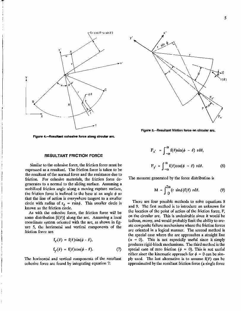
Figure 4.-Reaultant cohesive force along circular arc.

RESULTANT FRICTION FORCE

Similar to the cohesive force, the friction force must be expressed as a resultant. The friction force is taken to be the resultant of the normal force and the resistance due to friction. For cohesive materials, the friction force de­generates to a normal to the sliding surface. Assuming a mobilized friction angle along a moving rupture surface, the friction force is inclined to the base at an angle ¢> so that the line of action is everywhere tangent to a smaller circle with radius of r", = rsin¢>. This smaller circle is known as the friction circle.

As with the cohesive force, the friction force will be some distribution [f(O)] along the arc. Assuming a local coordinate system oriented with the arc, as shown in fig­ure 5, the horizontal and vertical components of the friction force are

fx'(O) = f(O)sin(¢> - 0),

fy( 0) = f( O)cos(¢> - 0). (7)

The horizontal and vertical components of the resultant cohesive force are found by integrating equation 7:

5

Figure 5.-Reaultant friction force on circular arc.

Fy' = J: f(O)cos(¢> - 0) rdO. (8)

The moment generated by the force distribution is

2a: M = J 0 (r sin¢»f(O) rdO. (9)

There are four possible methods to solve equations 8 and 9. The first method is to introduce an unknown for the location of the point of action of the friction force, F, on the circular arc. This is undesirable since it would be tedious, messy, and would probably limit the ability to cre­ate composite failure mechanisms where the friction forces are oriented in a logical manner. The second method is the special case where the arc approaches a straight line (a -+ 0). This is not especially useful since it simply produces rigid-block mechanisms. The third method is the special case of zero friction (¢> = 0). This is not useful either since the kinematic approach for ¢> = 0 can be sim­ply used. The last alternative is to assume f( 0) can be approximated by the resultant friction force (a single force

6

F located at 0', where -a ~ O' ~ a). This can be written mathematically via the Dirac delta function [S(x)]:

F = f(O)rS(O·). (10)

By substitution of equation 10 into equations 8 and 9, the resultant friction force is dermed in the local coordinate system,

Fx' = F sin(<p - 0"),

Fy' = F cos(<p - 0"),

M = Fr sin<p. (11)

Vardoulakis (5) solved equation 9 by making the assumption of a purely frictional soil (c = 0), such that equilibrium requires F = Fy., where there are no hori­zontal actuating forces. He then introduced a modifier (k) to the radius of the friction circle such that the moment Fkrsin<p is equivalent to equation 9.

In practice, the radius of the slip circle, r, and the location of the friction force, 0', will be known so that the only unknown in equation 11 is the value of the resultant, F. Furthermore, since the angle (<p - 0') is the orientation of the resultant, F, in the local coordinate system, a new angle ('7) can be dermed that is the orientation of the resultant, F, in the global coordinate system (x,y), which is done in the following section.

RESOLUTION OF FORCES

In the preceding two sections, it was shown how the stress distribution in the soil mass may be approximated by two resultant forces (F and T) on each circular arc. Creating a composite failure mechanism of three circular arcs (fig. 6) produces a failure mass of two soil wedges. Satisfying equilibrium of forces and moments for each soil

sin'73 sin°3 sin'72 sinO 2 0 0 COS'73 cos03 COS'72 cos02 0 0 0 0 sin'72 sinO 2 sin'7l sinO 1 0 0 COS'72 cos02 COS'71 cosO 1 0 0 0 0 ass ~ a16 a26 a36 a46 0 0

wedge requires six equilibrium equations for six unknowns (FlI TlI FlO TlO F3, T3)' In figure 6, FI and Ti are equilib­rium forces; 0, W LI and W R are actuating forces; ~, BlI D2, M, Ku and 0 1 are strategic points where the subscripts refer to the circular arc they lie on; '7;, 01, ai, and 8al are angles, and rl and rl are radii of the slip circle and friction circle, respectively.

In the case of a single friction circle (fig. 1), the system of forces consists of only three: friction force, F, cohesive force, T; and resultant actuating forces, 0 + W, where 0 is a load applied on the footing. In the case of only three force vectors, it is required that they must pass through a point to satisfy moments. In this case, the problem is simplified since the point of application of the friction force is fixed. In a two-wedge mechanism, there are a minimum of four forces acting on a wedge (fig. 7). In the case where the unit weight of the material is not zero, there will be five or more forces acting on each wedge. The significance of this is that the points of application of the friction forces are not specified. Thus, points 0;, which derme the locations of the friction forces, are said to be located off the center of each arc by an angle 8a;.

This introduces an additional three unknowns. The values of 8al will affect the orientations of the forces so that the force polygon (fig. 7) is not unique for a given configuration of the circle centers. Thus, it is necessary to optimize the angles, 8oc;, to determine the optimum ori­entations of the forces.

The matrix of equation 12 was formulated to solve the six remaining unknowns for the case of only vertically ap­plied loads and body forces. Notation is shown in fig­ure 6, where BI is the solution vector, Iljj are the matrix coefficients, e is the load eccentricity, and '71 and 01 are th~ orientations of the friction forces, Fi• and the cohesive forces, TI, respectively. By using equilibrium of forces of the global system and right wedge, and taking moments about point 0 3 and the second circle center,

F3 0+ WR + WL T3 0 F2 = 0+ WR T2 0 Fl Bs Tl B6 (12)

"'r. , 'I

7

Figure 6.-General system of forces on two-wedge mechanism.

where BS = WL (03x - GLx),

B6 = WR(C2x - GRJ + 0(C2x - b/2 - e),

and the moment arms /lss, ~, a16, a26 are the orthogonal distances from point C2 and 0 3 to the lines of action of the forces. The moment arms are positive for forces acting clockwise about the points and negative for forces acting counterclockwise. If the second circular arc is reversed, so it is convex instead of concave, then the parameters a36 and a46 are positive for forces acting counterclockwise and negative for forces acting clockwise. Points GL and GR are the centers of gravity of the left and right soil wedges.

KINEMATICS

For an admissible collapse mechanism, it must be pos­sible to describe the motion that takes place upon collapse. This can be presented in a hodograph.

The assumption of circular sliding surfaces made in the friction circle mechanism is only valid for no friction. Rigid wedges with friction along curved surfaces must have a surface with the shape of a logarithmic spiral to be admissible kinematically. Thus, the hodograph of the fric­tion circle method is rigorously correct for purely cohesive materials, but not for frictional materials (<fJ > 0). In the case of material with friction, the assumption must be made that the mechanism will slide along circular surfaces in order to apply the friction circle method; so kinematic admissibility is checked via the hodograph regardless of the value of friction.

8

Construction of the hodograph is based on drawing the velocities so that they are tangent to the sliding surfaces. For the friction circle, this can be accomplished most easily by drawing the velocities perpendicular to the circle radii. When the hodograph is completed, each solid wedge of soil is represented by an identically shaped wedge of arbitrary size rotated 9(JO.

The rotation of the wedge onto its perspective orienta­tion in the hodograph can be clockwise or counterclock­wise and can be determined by observing the relative

Q

Right wedge

Figure 7.-Force polygon for two-wedge mechanism.

motion of the wedge as it slides. For example, in figure SA, the general direction of the wedge is shown by the vector Vp, where V is the velocity at the point P. As the block slides along the arc it will rotate clockwise. Thus, the wedge is rotated 9(JO clockwise on the hodograph (flg.9A). Figures 8B and 9B show a counterclockwise rotation. The hodograph does not defme the actual mag­nitude of velocities, but only ratios of velocities: (Vp/V Q)' (V A/V Q)' etc.

The construction of the hodograph for a mechanism composed of multiple circles is more complex. Figure 10 shows a hodograph for the Prandtl mechanism. A step-by­step procedure is outlined for the construction of the hodograph for a three-circle mechanism:

1. A point is picked to represent zero velocity of fIXed earth (point C2h = ~h in figure 10). When the hodograph is completed, a vector drawn from the stationary point to soine other point, P, will represent the magnitude and orientation of the velocity vector of point P with respect to a stationary point.

2. A line perpendicular to the circle centerline is drawn, passing through the stationary point. Also, rays are drawn for the velocities of each point on the exterior sur­face (points ~, M, and DJ. This is done in figure 10 where rays rl..L; r2..L, r3..L, and r4..L on the hodograph cor­respond to rays rlO r2> r3, and r4 on the mechanism. It is assumed the centers of circles 2 and 3 are represented on the hodograph at the stationary point. This is because circles 2 and 3 defme exterior surfaces where there is a moving wedge sliding against fIXed material.

3. Centers of circles that defme interface surfaces be­tween two moving blocks do not have centers at the sta­tionary points. An arbitrary point, C1 h, on the perpendicu­lar to the circle centerline is selected to represent point C1• The location of this point determines the size of the

®

Figure 8.-RotaUng wedges. A, Clockwise rotaUonj B, counterclockwise rotaUon.

T

I I

9

®

A

Figure 9.-Hodographs of rotating wedges. A, Clockwise rotation; B, counterclockwise rotation.

Circle centerline

Figure 10.-Constructlon of hodograph for mechanism composed of three friction circles.

hodograph. Some other starting point could have been picked, but this one is convenient.

4. Rays rs..L and r6..L are drawn (perpendicular to rays rs and r6, respectively, passing through point C1h) to rep­resent relative velocities between the two moving blocks along the interface.

5. Strategic points can now be located on the hodo­graph. Point M, which must be located first, is at the in­tersection of rays r2nr6 on the left wedge and rays r3nr6 on the right wedge. Points Mi' and M3 h on the hodograph are at the corresponding perpendicular rays. Points Aah, B3h, Di', and Bi' can be located by rotating about the circle centers from point Mh to the appropriate ray the point lies on. (For example, point D2 lies on ray r4 and is connected to point M by an arc rotated about point C2. Thus, point D2h is located by rotating about point Ci' from point Mi'. The direction of rotation should be obvious if the perpendicular rays are drawn correctly.) The rotations derme four arcs on the hodograph that represent the three circular surfaces.

6. The remaining segments (AaB and D2B) can be connected, because the wedges in the hodograph should have the same shape as the wedges in the mechanism. The hodograph construction may be completed by scaling off relative distances, but in the case of figure 10, the segments are simply straight lines.

Once the hodograph is completed, the relative velocities of the forces can be measured by determining the point of application of the force on the body in the hodograph.

'I: I'

i: I I I,

!

I I ,-ii

: :

I'i

10

The direction and relative magnitude of the velocity of any point in the moving body can be measured by drawing a vector from the stationary point to the point of interest.

The velocities of all the friction forces are orthogonal to the force vectors for the case of q, = 0, such that no work is done by them on collapse. The velocity vectors of the cohesive forces are the velocities along the arcs. The relative velocity between the two moving wedges, every­where tangent to the interior surface, and its relative magnitude (V12) is the distance between the two wedges. The case where V12 = 0 is evident by a single wedge on the hodograph (M2 = M3, and B2 = B3) and circle centers of the mechanism C2 and ~, which correspond.

FACTORS OF SAFETY

Since methods for calculating the forces and velocities of the friction circle mechanisms have been developed, expressions for the relative stability of the mechanisms can now be developed. The friction circle method has adopted the factor of safety (FS) based on energies

FS = SD/SA, (13)

where SD is the dissipated energy of resisting forces and S A is the actuating energy of existing loads. By using different calculations for the energies (SD and SA), it is possible to formulate several expressions for the FS that are useful.

Friction

The friction circle method assumes the friction force is oriented at the angle of friction to the surface normal (see figures 1 and 5). This angle of friction that is used to represent a collapse mechanism is the critical angle of friction at failure (q,'). Since q,' differs from the measured angle of friction ( q, ) and q, , is required to orient the forces, it is necessary to separate FS's for friction and cohesion.

To obtain an FS consistent with equation 13, consider figure 11. The only actuating force is Q. The friction and cohesion resultants (F and T) can be determined, and the available shearing resistance to limit motion (T J is found by taking moments about the circle center,

T L r = Frsinq, + TR. (14)

Similarly, the equilibrium shearing resistance (Teq) is

Teq r = QL. (15)

L ~I

r sin cP I ~~~ I

\ I ~ \ \~

\ "" "" \ r \ ~ CPt-~ ~\

\ T

Figure 11.-Shearlng r.slstances.

Since the shearing resistances (T L and T eq) are dermed along the same surface, their displacements and velocities are equal and the FS (equation 13) reduces to a ratio of moments:

FS = TdTeq'

Substituting equations 5, 14, and 15 into 16 leads to

FS = Fsinq, + Ta/sina Q(L/r)

(16)

(17)

Equation 17 is not particularly useful since it cannot be solved explicitly. Since T is a function of F, F is a function of q" and q, is a function of FS, equation 17 is implicit. However, the expression must hold as cohesion becomes smaIl (T 40 0). Then, by equilibrium of forces, F must equal Q, be vertical, and be applied to a point on the slip circle directly under Q. In this case, (L/r) = sinq,' and equation 17 reduces to

(18)

Thus, tP' to be used in the analysis can be calculated from tP and a desired FS.

Cohe~ion

Since the factor of safety for friction (FS¢) must be incorporated into the geometry of the problem via equa­tion 11, it is only necessary to solve for the factor of safety for cohesion (FSc). The shearing resistances for tP = 0 can be written

TL = (Zar)c,

Teq r = TR. (19)

By using the location of the cohesive force resultant (equation 5) and the above expressions for the shearing resistances (equation 19), the FS (equation 16) can be expressed in the following usable form:

FSc = 2cr sina/T. (20)

This expression is valid for a single circular arc or can be taken as a summation of the numerator and denominator for an average FS for the mechanism.

An alternative to equation 20 is to express SA in terms of the actuating force, a, instead of the shearing resistance (Teq). Since the velocities of the forces are not equal, they are retained in the expressions for the energies

SA = a·yO. (21)

Substituting equation 21 into the FS (equation 13) leads to

(22)

The advantages of equation 22 are that the system of forces does not need to be solved and that it yields an upper-bound kinematic solution as postulated by Drucker (6). For composite failure mechanisms, the numerator is summed over the circular arcs and the denominator sum­med over each actuating force, which may also include the weights of the soil wedges in addition to the load, a. The disadvantage of equation 22 is that it is not affected by friction and thus always gives a solution for purely cohesive material.

11

Multisurface Mechanisms

During optimization of a mechanism, the configuration is adjusted such that the FS is minimized. Selection of a particular expression for the FS as an optimization pa­rameter 'can have a drastic influence on the optimization path. The FSc of equation 20 can be written for any indi­vidual surface generated by the i'th circle as

(23)

or as a summation for the mechanisms as a whole:

(24)

For frictional materials (tP > 0), the following assump­tions were postulated:

Assumption 1: p and c are fully mobilized on all surfaces where movement occurs.

Assumption 2: The FS is taken as a summation over surfaces where movement occurs.

Although the assumptions are straightforward, they have some implications that are not immediately obvious and are necessary to determine treatment of the interior circular arc.

Yelocities on exterior surfaces (arcs generated by cir­cles 2 and 3 on figure 6) are never zero except for the trivial case of no failure. Assuming limit load calculation, the FS on exterior surfaces is 1 (FS¢ = FSc = 1).

Yelocity on the interior surface (the arc generated by circle 1 in figure 6) may be zero if the centers of the second and third circles correspond. In this case, the subscript i takes on values 1,2 in equation 24. Since there is no movement, FSc1 ~1 (via equation 20) and FSi ~1 (via equation 18). A value of FS¢ > 1 means that the radius of the friction circle may be less than critical; i.e., o < r/ <r1sintP'. If the velocity between the two soil wedges along the interior surface is not zero, the sub­script i takes values 1,2,3.

OPTIMIZATION

Optimization of the average factor of safety for cohesion (FScav) resulted in erroneous results characterized by local FS's for individual arcs that varied widely and sometimes

i , \ 1\

i l

l

y:--

Ii I· , I." i

12

a wide variation in velocities of forces. Optimization of FSc·v involves two somewhat unrelated summations of minimizing the circle surfaces and maximizing the total cohesive forces necessary for equilibrium. Apparently, the maximum value for cohesive forces (}:; T J is that where two forces approach zero, forcing the third cohesive force to be large.

Optimization of FSc via kinetics (equation 22) did not experience such problems. The mechanism consistently converged to an optimum configuration. The stability of the optimization with equation 22 as an optimization pa­rameter is related to the influence of the hodograph.

Because use of equation 24 as an optimization param­eter was not sufficient to ensure a stable convergence, a third assumption was made:

Assumption 3: The minimum FS is found where the local FS's are also minimum and eqyal on each surface where movement occurs.

This assumption guarantees that the maximum amount of shearing resistance is fully utilized on each surface.

Assumption 3 was administered by periodically mini­mizing the largest local FS (FSJ and then converging the FS's such that they were equal. Convergence was done by choosing the maximum of I FSt - FS2 1, I FSt - FS3 1, and I FS2 - FS3 1 as the optimization parameter to be minimized. Thus, the optimization procedure adjusts the mechanism with respect to two separate parameters.

In some cases, optimization with respect to two sep­arate parameters leads to convergence toward two distinct configurations. This results in an oscillation between two convergence points and results in a solution that is not optimum and may be inadmissible if some local FS is < 1. Generally, the optimization was found to converge toward one distinct configuration. However, convergence was found to be slower and in some cases not possible as the friction angle was increased. Also, a large load, Q, with respect to soil weight was usually more likely to result in all positive forces (Fj and T J for a trial mechanism, so that convergence was faster and more likely to be completed.

The optimization scheme that was utilized in code OPTIC uses a modified term based on the direct search method proposed by Hooke and Jeeves (7). A flowchart of the direct search method is given in figure 12 for optimization of an arbitrary function. The base point and head point refer to the set of variables that derme the value of the function for the initial trial mechanism and the latest optimization. Otherwise, the flowcharts are somewhat generalized and self-explanatory.

The direct search method was selected since it does not require derivatives and it moves one parameter at a time

Switch to next

parameter

Reestablish head point

Reestablish head point

No Last parameter:x----------J

Yes

? Decrease I<E--__ ""No"-< Convergence Yes step size satisfactor~

Print

?

Figure 12.-Flowchart for Hooke and Jeeves method.

in search for an optimum configuration. Although other optimization schemes were not attempted, it is reasoned that a simplistic approach would be least affected by inadmissible configurations. Due to the vast amount of constraints in the friction circle method, the amount of admissible configurations is limited, making it difficult to optimize.

The FS for the friction circle may be expressed as a function:

where the variables t.Qj refer to modification factors to the locations of points Qj and the remaining variables are coordinates of the points, as shown in figure 6. The

optimization may be visualized as fmding the minimum value on a surface in nine-dimensional space. This surface for the friction circle method is found to be defmed over a fmite extent and usually contains numerous local minima. Furthermore, it appears to contain jagged edges and holes where configurations are not admissible.

A flowchart of the modified scheme utilized in code OPTIC (see appendix B) is given in figure 13. In the modified scheme, the locations of the. forces, by adjusting the value of b.Oli, are moved first so that the optimum force polygon is considered for each configuration of circles. Then point ~x is optimized for each movement of points C1 and Cz• This is done because only point ~ is

Yes

Start subroutine

1

Better optimization parameter

?

Better Yes optimization

parameter ?

No

Move A 3X backward

No

(, Return

13

needed to control the shape of the left wedge once the shape of the right wedge has been determined by points C1 and C2• Thus, in effect, the optimum configuration of the left wedge is considered for each trial configuration of the right wedge.

The method is demonstrated in a computer program OPTIC, which is written in compiled BASIC and is rel­atively user friendly (see appendix B). Run time of the program varies widely, dependent on the input param­eters. However, most solutions are obtained in 2 to 3 min, running on an IBM Corp. compatible personal computer equipped with an Intel 80286 chip and 80287 math coprocessor, both having a clock speed of 16 MHz.

Yes Any

points moved?

tart subroutine

j

Yes Any

points moved

No

Yes

Start subroutine

1

Any points

moved? No

Swich optimization parameter Minimization 1+-----; to conver ence

Yes Stop

Figure 13.-Flowchart for optimization procedure In code OPTIC.

i i !

! i

i i ; \

r I

14

ECCENTRIC LOADS

Because eccentric loads will tend to cause rotational failure mechanisms, the friction circle method is a useful method for investigating the effect of eccentricities.

The commonly adopted method of treating eccentricities in foundation design is to assume the footing to be a width, bo - 2e, where bo is the actual width of the footing. As shown in figure 14, the assumed footing remains centrally loaded since a width of 2e is assumed not to exist. If (q/ c r is the nondimensionalload capacity of the eccentrically loaded footing over a width, bo (fig. 14) and (q/c)o is the nondimensionalload capacity of a centrally loaded footing over a width, bo (not shown), then the method of equivalent footings leads to the expression

I (q/c)* = (q/c)o[1 - 2e/bol· I (26)

Similar expressions can be derived from the friction circle method.

SINGLE-CIRCLE MECHANISM WITHOUT UPLIFT

The effect of eccentric loads is considered here for a strip footing that is not allowed to tilt up. The roller (shown in figure 15A) allows the left edge of the footing to translate horizontally, but not vertically. This con­straint considered in the hodograph (fig. 15B) requires that the center of the circle must be above the edge of the footing.

Consider a purely cohesive soil so that the friction force, F, passes through the circle center. To satisfy moments, the friction force must also pass through the intersection of the force vectors, 0 and T. Then, from the geometry of the mechanism (fig. 15A),

tane = R/(b/2 + e), (27)

and from the hodograph (fig. 15B),

Vo b/2 sino: = 2 - .".....,~-Vc b/2 + e'

(28)

and from the force polygon (fig. 15C),

tane = OfT. (29)

Expressing the load as a resultant of the distributed load, 0 = qb, the FS can be obtained by substituting equation 28 in the kinematic expression (equation 22) or

by substituting equations 27 and 29 into the force equilib­rium expression (equation 20). Either method reduces to

q = -:-_40:~r--:-_ c (b + 2e )sino: .

(30)

Making use of the relation sino: = b/r, equation 30 can be expressed in a form analogous to the expression derived by consideration of equivalent footings:

(31) where

(32)

Equation 31 is of a form similar to the equivalent footings expression (equation 26). (Incidentally, an opti­mum value of (q/c)o ~ 5.52 is obtained from a value of 0: ~ 1.1656 radians.)

SINGLE-CIRCLE MECHANISM WITH UPLIFT

If the roller support is removed from the scenario in figure 15A so that footing uplift is allowed, the circle center is not necessarily above the edge of the actual foot­ing. Here, the assumption is made that the circle center lies a distance 2e to the right of the footing edge, as shown in figure 1M. The hodograph is shown in figure 16B.

The friction force again passes through the circle center and the intersection of force vectors, 0 and T. From the geometry of the mechanism,

tane = R/(b/2 - e). (33)

The force polygon (fig. 16C) is the same as the previous case without uplift.

The ultimate load is obtained by substituting equa­tions 29 and 33 into the force equilibrium expression for the FS (equation 20),

(q/c) = 4o:r/bsino:. (34)

Substituting sino: = (b - 2e) /r into equation 34 and re­arranging leads to the very same expression derived con­sidering equivalent footings (equation 26). This is to be expected since the size of the friction circle (fig. 1M) is proportional to the footing width by the same ratio as the equivalent footing (refer to discussion concerning equation 26).

I. I I I I-e I

Q

14-----b -------.I ~--------bo-------~

Figure 14.-Equlvalent footings.

® © Figure 15.-Slngle-clrcle mechanism without uplift. A, Force

diagram; B, hodograph; C, force polygon.

15

L..-_.L-4-.. T

o

q

® © Figure 16.-Slngle-circle mechanism with uplift. A, Force

diagram; B, hodograph; C, force polygon.

THREE-CIRCLE MECHANISM

Code OPTIC was used to compute results for the ec­centrically loaded footing by the kinematic method. The three-circle mechanism was allowed to move freely, unlike the single-circle examples that were computed analytically, where a mechanism is partially assumed by specifying the horizontal coordinate of the circle center. The interesting result of the three-circle mechanism is that, over a moderate range of eccentricities, it converges to the single­circle mechanism with uplift (as shown in figure 1M).

The equations derived from the equivalent footing assumption or single circle with uplift (equation 26) and

I

i

i!

16

single circle without uplift (equation 31) are plotted in figure 17. Comparison shows that when the footing is restrained such that it does not rotate upward, a significant increase in strength occurs.

The three-circle mechanism solution to Prandtl's prob­lem is (q/c) ~ 5.30, which is closer to the closed form solution of (q/c) = 2 + 11' than the single-circle solution (q/c) ~ 5.52. However, for eccentric loads, the three­circle mechanism converges to the equivalent footings expression (equation 26). The transition point where the single circle and composite mechanism diverge was found to be (elb) ~ 0.09. The mechanisms obtained from the convergence points of code OPTIC for eccentricities of e = 0 and (elb) ~ 0.09 are shown in figures 1&4. and 188, respectively. The improvement of the solution by the three-circle mechanism over equation 26, for small ec­centricities of (e/b) < 0.9, is shown in the upper left portion of figure 17.

The three-circle mechanism also diverges from equa­tion 26 for eccentricities (e/b) > 0.25. This anomaly is produced by a constraint in the OPTIC code. The failure surface termination point A3 (see figure 6) is not allowed under the footing, so that the failure surface runs a minimum length of the footing. However, this anomaly lies in the range of eccentricities that is typically not allowable in practice.

The conclusion is that a factor for bearing-capacity reduction, based on the three-circle mechanism, due to eccentric loads would result in deviations from the present method that would be neglible. Also, the present method of equiValent footings is on the conservative side.

U ..... g

~ ~ 0: « ()

(!l z cc « w co

~ ~ ~

~ ~Q ~Q I I I I I I I I I I I I

6.0 I I I

Prandtl solution = 2 + .".

4.0

3.0 Equation 26

~, ... ;-OPTIC

.... 2.0 'a... ...

"''0... ....... "'0... ......

Typical maximum

1.0 allowable eccentricity

(e/b) = 0.25

0 0.1 0.2 0.3 0.4 0.5 ECCENTRICITY (e/b)

Flgur. 17.-Effect of eccentricity on bearing capacity.

®

q/c=4.53 e/b = 0.09

Figure 18.-Fallure mechanisms of strip footings. A, Centrally loaded; B, eccentrically loaded.

17

EFFECT OF EMBEDMENT

Calculation of ultimate load of foundations may be given by the Buisman-Terzaghi equation (8):

q = cNc + q,Nq + Y2'YbN'Y' (35)

where 'Y is the unit weight and N is the bearing capacity factor. Values of No> Nq• and N'Y' as given in table 1 are calculated by

Nq = efrtan4>tan2(1t/4 + t/J/2) ,

Nc = (Nq - l)cott/J,

N'Y = 2(Nq + l)tan,p, (36)

and are said to lead to errors not exceeding 17 to 20 pct for frictional materials (30° < t/J < 40°), while the error is zero for cohesive materials. Equation 36 represents curve fits to data that are obtained by the method of char­acteristics. The analyses by method of characteristics assume a mechanism, as shown in figure 19, where the footing is even with the ground and there is a distributed surcharge load, qo.

Table 1.-Partlal listing of bearing capacity factors

Friction angle No (4)), deg

Nq N'Y

0 ........... , ..... 5.14 1.00 0.00 5 ... , ........... 6.49 1.57 .45 10 .............. 8.35 2.47 1.22 20 .............. 14.83 6.40 5.39 30 •••• I ••••••••• 30.14 18.40 22.40 40 .............. 75.31 64.20 109.41

In reality, the foundation is rarely even with the ground surface as posed in figure 19. For embedded footings, as shown in figure 20, the soil weight over the depth of em­bedment (0) is taken as the surcharge load, q, = 'YO. With this simplification, the shearing resistance between the foundation and soil (segment AD in figure 20) and between the overburden and supported soil (segment BC in figure 20) is neglected so that the bearing capacity factor (No) becomes conservative as 6 is increased. The composite friction circle method does take account of this additional shearing resistance, which· is a particular ad­vantage of the friction circle method.

An attempt was made to establish a relationship be­tween ultimate load and O. However, this is complicated by two fundamental problems. The fIrst problem is that, while the bearing capacity factors are approximated as a function of the friction angle only, the effect of embed­ment (influenced by the shearing resistance along the neglected segments AD and BC of figure 20) is dependent on both friction and cohesion. The second problem is the inherent complication associated with the friction circle method as the cohesion becomes small, which places a limitation on the range of values for soil strength where the effect of embedment could be investigated. Thus, establishing a relationship between ultimate load and embedment over a broad range of c and ,p could take a considerable amount of time and effort.

Although the composite friction circle method becomes conservative as the cohesion approaches zero, this does not reduce the applicability of the method for higher values of cohesion. The calculation of bearing capacity for a partic­ular problem is a much easier task than trying to fit a curve to the nonlinear variation of bearing capacity as a function of embedment.

Figure 19.--Aasumed mechanism for bearing capacity factors.

1 " ,

Figure 2O.-Analyal. of embedded footing with bearing capacity factor ••

BEARING CAPACITY CALCULATIONS NEAR SLOPES

The friction circle method can be used for bearing capacity calculations of footings that are embedded, have eccentric and/or inclined loads, and are near slopes. Some demonstrations of the OPTIC code are given here.

Comparison is made with the kinematic rigid-block method. Papanastiou (9) used a mechanism composed of two rigid blocks (shown in figure 21) to produce a dimensionless nomograph for a centrally loaded surface footing near a slope. The limit load, Qu, is then a func­tion of the soil properties, "I, c, and 4>; the footing width, b; and the slope angle (fJ). For constant values Qf fJ and 4>, the dimensionless term Qhb2 varies almost linearly with the dimensionless term chb. Typical values of "I = 15 kN/m3

, 4> = 20°, and b = 5 m were chosen, and fJ was varied from 0° to 50° in increments of 10°. The nomograph given by Papanastiou was reproduced and results from the composite friction circle method were superimposed on it in figure 22.

The major disadvantage of Taylor's friction circle method (composed of a single circle for slope stability without any surcharge loads) is that when 4> exceeds fJ, the equilibrium cohesion necessary to maintain stability is negative. This violates the kinematics of the problem since a negative cohesion force does not oppose motion; i.e., it cannot be developed for the assumed collapse mechanism. This basic problem is also inherent to the composite

friction circle method with three circles. For small values of cohesion it becomes increasingly difficult to fmd a mechanism where all three equilibrium cohesion forces are positive. Thus, the result is that the rigid-block mech­anism is typically lower bound to the composite fiction circle method for values of (chb) < 0.2 and 4> = 20°.

In the upper right portion of the nomograph, where fJ's are small and equilibrium cohesive forces are large, the friction circle showed a significant improvement over the rigid two-block mechanism. However, this is primarily due to the limiting ability of only two blocks to conform to a smooth failure surface for small fJ's. A rigid-block mechanism composed of four or more blocks showed a significant improvement over the two-block mechanism for fJ's < ZOO and was slightly lower bound to the composite friction circle method.

The example of the collapse mechanism in the nomo­graph does not take advantage of several features of the composite friction circle method. A slightly more complex problem of an embedded foundation with an eccentric load is analyzed in figure 23. This is an example where many methods, such as the method of slices, would be limited in their ability to assess the influence of the embedment and eccentric loads. With only slight modifi­cation, the OPTIC code could also consider inclined eccentric loads.

....... N .0

.t-O" ...... 0 <§ .:J

Figure 21.--Klnematlc rigid-block mechanism.

25r----------.----------r----------.----------~----------.--------~

20

15

10

5

0.2

cp=20°

0.4 0.6

COHESION (c/yb)

0.8

10° ~ -------- 20° -- ---~ 30° ::::;.-- --- ;..;.--

1.0 1.2

Figure 22.-Comparl80n of bearing capacity factor. by two-wedge rigid-block method and two-wedge friction circle method.

19

I.

; ;

I

Ii' I

i' i,'

I I:

Iii,

'I "I

20

Stationary point

! 72 607

486

y. C. cp = 15. 87.5. 200

Figure 23.-Collapn mechanism for embedded foundation with eccentric load near slope.

The weight of the foundation has been neglected in the OPTIC code. It is assumed that the weight of the founda­tion is included in the load, Q. Since the foundation is assumed to act as an integral portion of the right soil

wedge, a unit weight of concrete could be incorporated into the code. Although, for large loads, this would probably have a negligible influence.

CONCLUSIONS

A method for utilizing composite failure mechanisms constructed of three friction circles is presented. This method can be used for determining stability of some simple structures on homogeneous soils. The method is an extension of the well-known Taylor friction circle method and follows the work of Gudehus (4). The method has the following characteristics:

1. The FS is assumed to be equal to 1 for limit analysis. This effectively makes the use of the kinematic FS based on energy equilibrium, used in derivation of the friction circle method, irrelevant, so that the more commonly adopted FS,

FS = c/c' = tan</Jltan</J', (37)

may be utilized.

2. Due to constraints of the method, it is not possible to optimize the mechanism and converge toward a mini­mum FS. Thus, the value of cohesion at limiting equilib­rium is determined as an alternative. If the cohesion is known a priori, as is usually the case, a limit load must be determined by trial and error.

3. The value of cohesion in a soil mass cannot be nega­tive. Since the method calculates the value of cohesion at limiting equilibrium, it can only be used when a value of cohesion > 0 is required for stability.

4. Although the method generally utilizes equilibrium of forces to calculate the FS' an FS based on kinematics can be utilized for </J = O. In this case, the method yields an upper-bound kinematic solution as postulated by Drucker (6). This FS based on kinetics is always less than or equal to the FS based on equilibrium of forces.

Comparison of bearing capacities with other methods shows the method yields results that are somewhat con­servative for small values of cohesion and converge closer to closed-form solutions for larger values of cohesion with respect to soil weight and friction angle. The major hindrances to the method are local minima obtained in optimization, requirement of a homogeneous soil mass, and the difficulty of obtaining an initial mechanism as a starting point prior to optimization. Presently, one must obtain input parameters by using a compass and straight edge and drawing an admissible mechanism on paper.

-------·r

21

There are several areas for further research and improvements in the OPTIC code. The weaknesses of the code include the optimization procedure and searching routines for an admissible mechanism, which are areas for possible refmement. Possible additions to the code include horizontal loads on the footing. An option of horizontal gravitational loads on the footing would enable the code to be used for analyses of retaining walls. Inclusion of the weight of concrete in the foundation would allow analysis of gravity walls and dams.

REFERENCES

1. Degroot, R. L. Dump Point Stability Analysis. M.S. Thesis, Univ. MN, 1986, 66 pp.

2. Crum, D. A. Application of a Full Scale Dump Point Stability Experiment to Engineering Analysis. M.Ge.E. Thesis, Univ. MN, 1988, 77pp.

3. Taylor, D. W. Fundamentals of Soil Mechanics. Wiley, 1948, 700 pp.

4. Gudehus, G. Engineering Approximations for Some Stability Problems in Geomechanics. Paper in Advances in Analysis of Geotechnical Instabilities. Univ. Waterloo Press, 1978, pp. 1-23.

5. Vardoulakis, I. Lecture Foundation Engineering. Univ. MN, Minneapolis, MN, 1985-90, 100 pp.; available from I. Vardoulakis, Univ.MN.

6. Drucker, D. C., H. J. Greenberg, and W. Prager. Extended Limit Design Theorems for Continuous Media. Q. Appl. Math., v. 9, No.4, 1952, pp. 381-389.

7. Kuester, J. L., and J. H. Mize. Optimization Techniques With FORTRAN. McGraw-Hili, 1973, 256 pp.

8. Winterkorn, H. F., and H. Y. Fang. Foundation Engineering Handbook. Van Nostrand Reinhold, 1975, 75 pp.

9. Papanastiou, P. C. Passive Earth Pressure and Bearing Capacity Computations With Microcomputers. M.S. Thesis, Univ. MN, 1986, 76pp.

BIBLIOGRAPHY

Huang, Y. H., and C. M. Avery. Stability of Slopes by Logarithmic Spiral Method. J. Geotech. Eng., ASCE GT1, v. 102, Jan. 1976, pp.41-49.

Huntington, W. C. Earth Pressures and Retaining Walls. Wiley, 1957, 534 pp.

i i

i

II;.', 'I

I,

i :

I'

22

APPENDIX A.-NOTATION1

ENGLISH (x,y) coordinates in global system (X:y') coordinates in local system

A,B,C,D,M,P points

Cl;j matrix coefficients GREEK b width of footing [DISTANCE] c cohesion in soil [FORCE divided by a angle of half the arc defined by slip circle

AREA] flaj angle locating point Qj

e eccentricity p slope angle F j resultant of normal force and frictional S depth of embedment [DISTANCE]

resistance [FORCE] S(x) Dirac delta function FS factor of safety 'Y unit weight [FORCE divided by VOLUME] f(O) frictional resistance and normal stress as 111 orientation of friction resultant, Fi

function of position on slip circle q, internal angle of friction of the soil [FORCE divided by AREA] 0 angle measured counterclockwise from

G center of gravity center of slip circle

~ intersection points of resultant cohesion 01 orientation of cohesion resultant, T j

force T and central bisector of circular arc k a constant SUBSCRIPTS L length [DISTANCE] M moment [FORCE multiplied by A,P points

DISTANCE] c cohesion N bearing capacity factor eq equilibrium, from actuating forces n outward normal iJ unspecified circle or matrix coefficient index a load [FORCE] L limiting, from dissipating forces OJ intersection points of force vectors F j and L,R left and right soil wedge

TI 0 initial state q distributed load [FORCE divided by a load

AREA] q surcharge load R radial distance to cohesion resultant, T j x coordinate along x axis, horizontal

[DISTANCE] y coordinate along y axis, vertical r l radius of slip circle or ray related to 1,2,3 one of three circles

hodograph [DISTANCE] 1-6 matrix or solution vector coefficients Ti tangential force due to cohesion [FORCE] q, friction t constant value of cohesive shear stress

[FORCE divided by AREA] SUPERSCRIPTS t(O) cohesive shear stress as function of position

on slip circle [FORCE divided by AREA] av average (u,v) coordinates in local system h hodograph V velocity [DISTANCE divided by TIME] ... critical, at point of failure or having W weight of soil wedge [FORCE] singularity point

local lTenns in brackets define dimensions of selected variables. .1. perpendicular

23

APPENDIX B.-GlOSSARY

Critical.-The point at which the stability of the struc­ture changes from a stable, safe state of being to a col­lapse, where the factor of safety is 1.

Force equilibrium.-Refers to calculations based on ad­missible and limiting states of stress in the structure.

Hodograph.-A velocity diagram where the relative ve­locities of moving objects are mapped.

Kinematic (moving).-Refers to calculations based on velocities.

Limit analysis .-Analysis of a structure at its limiting or critical state of impending failure.

Lower bound.-A value that is on the "safe" side. A method that yields an ultimate load less than some base value, where the base value is taken to be the "true value" if not otherwise specified.

Nomograph.-A graph containing multiple curves, con­structed for use in determining values of some unknown based on two other known values.

Upper bound.-A value that is on the "unsafe" side. A method that yields an ultimate load higher than some base value, where the base value is taken to be the "true value" if not otherwise specified.

":: I

I i

I:

i I I i,

t

~'l

i!'I: \ i .

I

'i

24

APPENDIX C.-OPTIC CODE LISTING

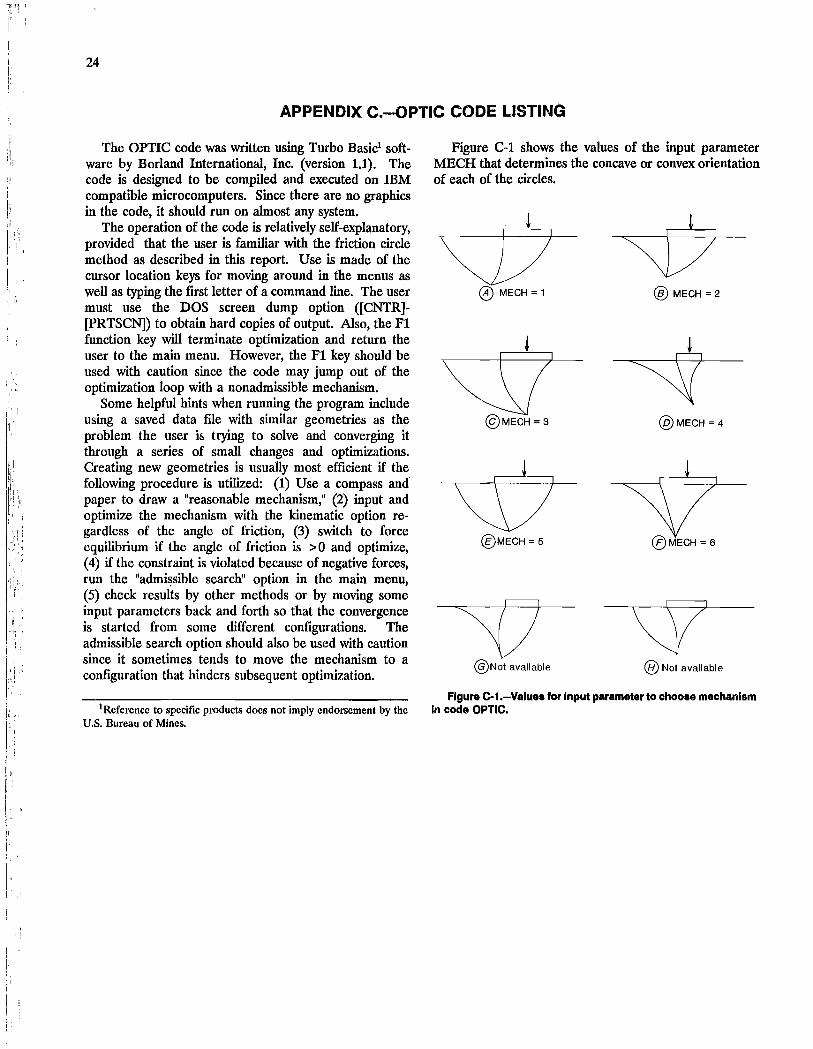
The OPTIC code was written using Turbo Basicl soft­ware by Borland International, Inc. (version 1.1). The code is designed to be compiled and executed on IBM compatible microcomputers. Since there are no graphics in the code, it should run on almost any system.

The operation of the code is relatively self-explanatory, provided that the user is familiar with the friction circle method as described in this report. Use is made of the cursor location keys for moving around in the menus as well as typing the first letter of a command line. The user must use the DOS screen dump option ([CNTR]­[PRTSCN) to obtain hard copies of output. Also, the Fl function key will terminate optimization and return the user to the main menu. However, the Fl key should be used with caution since the code may jump out of the optimization loop with a nonadmissible mechanism.

Some helpful hints when running the program include using a saved data file with similar geometries as the problem the user is trying to solve and converging it through a series of small changes and optimizations. Creating new geometries is usually most efficient if the following procedure is utilized: (1) Use a compass and paper to draw a "reasonable mechanism," (2) input and optimize the mechanism with the kinematic option re­gardless of the angle of friction, (3) switch to force equilibrium if the angle of friction is > 0 and optimize, (4) if the constraint is violated because of negative forces, run the "admi~sible search" option in the main menu, (5) check results by other methods or by moving some input parameters back and forth so that the convergence is started from some different configurations. The admissible search option should also be used with caution since it sometimes tends to move the mechanism to a configuration that hinders subsequent optimization.

1 Reference to specific products does not imply endorsement by the U.S. Bureau of Mines.

Figure C-l shows the values of the input parameter MECH that determines the concave or convex orientation of each of the circles.

Q/ o MECH = 1 ® MECH =2

@MECH=3 @MECH=4

®MECH =5

~ @Not available ® Not available

Figure C-1.-Values for Input parameter to choose mechanism In code OPTIC.

'Foundation-Slope Stability Program 'spring, 1989 CLS : PRINT Program "OPTIC", a "FOUNDATION - SLOPE STABILITY PROGRAM" PRINT "This program uses a Friction Circle method consisting of 3 circles." PRINT "It calculates the optimum limit load by adjusting the value ot" PRINT "cohesion for a given factor of safety. The program assumes a footing" PRINT "near an infinite slope." PRINT ,,--------------------------------------------------------------------" 1 V$ = INKEY$ : IF V$ = "" THEN 1

OPTION BASE 1 : KEY OFF DIM LX(19), LY(19), VAR(19), MAT(7,6), B(6), X(6), CH$(13) DIM PX(20), PY(20), A(8), GX(8), GY(8), DELTA(4), FS(4), 0(4) PI=4*ATN(1) : RNNUM=O : FSCOH=l : KINMAT=O : TRAP$ = "OFF' ON ERROR GOTO 9900 KEY(l) ON : ON KEY(l) GOSUB Kbreak GOTO 150

,------------------------------------------------------------------~-----------

Kbreak: RETURN 150

Okey: IF (ROW=8) OR (ROW=9) THEN

IF TRAP$= "ON" THEN COLOR 10,0 : LOCATE LY(8),LX(8) : PRINT CH$(8) COLOR 12,0 : LOCATE LY(9),LX(9) : PRINT CH$(9)

ELSE COLOR 10,0 : LOCATE L Y(9),LX(9) : PRINT CH$(9) COLOR 12,0 : LOCATE LY(8),LX(8) : PRINT CH$(8)

END IF ELSEIF (ROW = 10) OR (ROW = 11) THEN

IF KINMAT= 1 THEN COLOR 10,0 : LOCATE LY(10),LX(10) : PRINT CH$(10) COLOR 12,0 : LOCATE LY(l1),LX(l1) : PRINT CH$(l1)

ELSE COLOR 10,0 : LOCATE LY(l1),LX(l1) : PRINT CH$(l1) COLOR 12,0 : LOCATE LY(10),LX(10) : PRINT CH$(10)

END IF END IF RETURN

Upkey: KEY(l1) OFF : GOSUB Okey : LROW = ROW : ROW = ROW-1 IF (ROW=8) OR (ROW = 10) THEN ROW = ROW-1 IF (ROW =9) AND (TRAP$ = "ON") THEN ROW = 8 IF (ROW = 11) AND (KINMAT=l) THEN ROW=10 IF ROW = 0 THEN ROW = 1 COLOR 0,7 : LOCATE LY(ROW),LX(R0W) : PRINT CH$(ROW) IF (ROW>9) OR (ROW<7) THEN

COLOR 12,0 : LOCATE LY(LROW),LX(LROW) : PRINT CH$(LROW) END IF COLOR 7,0 : KEY(l1) ON

25

i,1 I' I'

~rl

f' ,

II '

"

26

RETURN 400

Downkey: KEY(14) OFF : GOSUB Okey : LROW = ROW : ROW = ROW + 1 IF (ROW<9) THEN COLOR 12,0: LOCATE LY(LROW),LX(LROW) : PRINT CH$(LROW) IF (ROW=9) OR (ROW = 11) THEN ROW = ROW+1 IF (ROW =8) AND (TRAP$= "OFF') THEN ROW = 9 IF (ROW = 10) AND (KINMAT=O) THEN ROW=l1 IF ROW = 13 THEN ROW = 12 COLOR 0,7 : LOCATE LY(ROW),LX(ROW) : PRINT CH$(ROW) COLOR 7,0 : KEY(14) ON RETURN 400

400 IF (ROW=7) OR (ROW=12) THEN LROW=ROW IF (ROW = 12) OR (ROW<8) THEN 160 KEY(12) ON : KEY(13) ON

Trap: GOTO Trap:

Sideway: LROW = ROW : ROW = ROW + 1 IF (ROW = 10) OR (ROW = 12) THEN ROW = ROW - 2 RETURN 160

,--------------_ .......... _-_ ... _-------------------------------------------------------------------------

LROW = 1 150 CLS GOSUB8000 KEY(l1) ON KEY(12) ON KEY(13) ON KEY(14) ON

ROW = 1 '[Main menu screen setup] ON KEY(l1) GOSUB Upkcy ON KEY(12) GOSUB Sideway ON KEY(13) GOSUB Sideway ON KEY(14) GOSUB Downkey

160 COLOR 12,0 : LOCATE LY(LROW),LX(LROW) COLOR 0,7 : LOCATE LY(ROW),LX(ROW) COLOR 7,0

162 V$ = INKEY$ : IF V$ = 1111 THEN 162 IF LEN(V$) = 2 THEN V$ = RIGHT$(V$,1) IF (V$ = "I") OR (V$ = "i") THEN

LROW = ROW : ROW = 1 : GOTO 160 ELSEIF (V$="D") OR (V$="d") THEN

LROW = ROW : ROW = 2 : GOTO 160 ELSEIF (V$ = liP') OR (V$ = "f') THEN

LROW = ROW : ROW = 3 : GOTO 160 ELSEIF (V$ = "R") OR (V$ = "r") THEN

LROW = ROW : ROW = 4 : GOTO 160 ELSEIF (V$="O") OR (V$="O") THEN

LROW = ROW : ROW = 5 : GOTO 160 ELSEIF (V$ = "A") OR (V$ = "a") THEN

LROW = ROW : ROW = 6 : GOTO 160 ELSEIF (V$ = "P") OR (V$ = "p") THEN

LROW = ROW : ROW = 7 : GOTO 160 ELSEIF (V$ = "2") THEN

PRINT CH$(LROW) PRINT CH$(ROW)

f

LROW = ROW : ROW = 8 : GOTO 160 ELSEIF (V$ = "3") THEN

LROW = ROW : ROW = 9 : GOTO 160 ELSEIF (V$ = "K") OR (V$ = "k") THEN

LROW = ROW : ROW = 10 : GOTO 160 ELSEIF (V$ = "L") OR (V$ = "I") THEN

LROW = ROW : ROW = 11 : GOTO 160 ELSEIF (V$="E") OR (V$="e") THEN

LROW = ROW : ROW = 12: GOTO 160 ELSEIF ASC(V$) = 13 THEN

ON ROW GOTO 201,202,203,204,205,206,207,208,208,210,210,212 201 GOSUB 4000 : GOTO 150 'Interactive Input 202 GOSUB 4100 : GOTO 150 'Data me input 203 GOSUB 4200 : GOTO 150 'File save 204 CLS: RN$ = "RUN" : GOSUB 6300 '[INITIALIZE]

Trap3:

GOSUB 1000 : GOSUB 1000 IF LIM = 0 THEN PRINT"*** Constraint #";cnum;" Violated ******" PRINT"Kine. = ";FSKIN PRINT"Limi. = ";FSCL1,FSCL2,FSCL3

IF INKEY$ = "" THEN Trap3: GOTO 150

205 RN$ = "OPTI" : GOSUB 2000 : GOTO 150 206 RN$ = "SEARCH" : GOSUB 2200 : GOTO 150 207 KEY(l1) OFF: KEY(12) OFF: KEY(13) OFF: KEY(14) OFF

GOSUB 5000 : GOTO 150 'Print results 208 IF ROW = 8 THEN

TRAP$ = "ON" COLOR 10,0 : LOCATE LY(8),LX(8) : PRINT CH$(8) COLOR 12,0 : LOCATE LY(9),LX(9) : PRINT CH$(9)

ELSE 'row=9 TRAP$ = "OFF" COLOR 12,0 : LOCATE LY(8),LX(8) PRINT CH$(8) COLOR 10,0 : LOCATE LY(9),LX(9) PRINT CH$(9)

END IF GOTO 162

210 IF ROW = 10 THEN KINMAT = 1 COLOR 10,0 : LOCATE LY(10),LX(10) : PRINT CH$(10) COLOR 12,0 : LOCATE LY(l1),LX(l1) : PRINT CH$(l1) COLOR 7,0

ELSE 'row=l1 KINMAT = 0 COLOR 12,0 LOCATE LY(10),LX(1O) PRINT CH$(10) COLOR 10,0 : LOCATE LY(l1),LX(l1) PRINT CH$(l1) COLOR 7,0

END IF GOTO 162

212 STOP: END ELSE

LOCATE 23,20: PRINT "Huh?" END IF

GOTO 160

-------------:"

27

"I Ii, : ~ !

Ii , l

[

11

-pr:;1 ;''',. '

28

I I

, I ,********************************************************************************************************

I !t

1000 'Subroutine FACfOR KEY(1) ON : LIM = 1 : RNNUM=RNNUM + 1 IF A3X = > BF THEN LIM=O : CNUM=6 : GOTO 1987 IF C1 Y = C2Y THEN LIM = 0 : CNUM =0 : GOTO 1987

'Constraint #6

,---------------------------- Compute Strategic Points & Radii ----------------------------BlX = BF B1Y = 0 B2X = BlX + BW: B2Y = -EMBED SELECf CASE MECH CASE 1

IF ClX>BlX OR C2X>B2X THEN LIM=O CNUM=8 GOTO 1987 CASE 2

IF ClX>BlX OR C2X>B2X THEN LIM=O CNUM=8 GOTO 1987 CASE 3

IF ClX<BlX OR C2X<B2X THEN LIM=O CNUM=8 GOTO 1987 CASE 4

IF ClX<BlX OR C2X<B2X THEN LIM=O CNUM=8 GOTO 1987 CASES

IF ClX<BlX OR C2X>B2X THEN LIM=O CNUM=8 GOTO 1987 CASE 6

IF ClX>BlX OR C2X<B2X THEN LIM=O CNUM=8 GOTO 1987 END SELECf

A3Y = A3X*TAN(BETA) R1=SQR«ClX-BlX)"2 + (C1Y-B1Y)"2) R2=SQR«C2X-B2X)"2 + (C2Y-B2y)"2)

Y1 = (C2X-ClX)/(C2Y-C1Y) : Y3 = Y1"2 + 1 Y2 = (ClX"2 - R1"2 - C2X"2 + R2"2 + (C2Y-C1Y)"2)/(2*(C2Y-C1Y» Y4 = 2*Y1 *Y2 - 2*C2X : Y5 = Y2"2 - R2"2 + C2X"2 IF (Y4"2 - 4*Y3*Y5)<0 THEN LIM=O : CNUM=1 : GOTO 1987 'Constraint #1 IF EMBED >0 THEN

IF MECH=3 OR MECH=4 THEN Y1 = SQR«ClX-BlX)"2 + (C1Y+EMBED)"2) IF Y1>R1 THEN LIM=O: CNUM=O: GOTO 1987 'thru foundation

END IF END IF

SELECf CASE MECH CASE 1

MX = (-Y4 + SQR(Y4"2 - 4*Y3*Y5»/(2*Y3) CASE 2

MX = (-Y4 + SQR(Y4"2 - 4*Y3*Y5»/(2*Y3) CASE 3

MX = (-Y4 - SQR(Y4"2 - 4*Y3*Y5»/(2*Y3) CASE 4

MX = (-Y4 - SQR(Y4"2 4*Y3*Y5»/(2*Y3) CASE 5

MX = (-Y4 - SQR(Y4"2 - 4*Y3*Y5»/(2*Y3)

CASE 6 MX = (-V4 + SQR(V4"2 - 4*V3*V5»/(2*V3)

END SELEeI'

TEMP = R1"2 - (MX-ClX)"2 : IF TEMP < 0 THEN LIM = 0 : GOTO 1987 My = C1y + SQR(TEMP)

1010 Vl = SQR«Mx-C2x)"2 + (My-C2y)"2) - R2 : IF INT(ABS(Vl*l00»=0 THEN 1011 My = Cly - SQR(TEMP) : GOTO 1010

1011 'endif

IF MY>-EMBED THEN LIM=O CNUM=2 : GOTO 1987 'Constraint #2 IF MY>MX*TAN(BETA) THEN LIM=O : CNUM=3 GOTO 1987 'Constraint #3

2 IF (TRAP$="ON") AND (BETA=O) THEN C3X = C2X : C3Y = C2Y A3X = C2X - SQR(R2"2 - C2Y"2) : A3Y = 0

ELSEIF TRAP$ = liON" THEN C3X = C2X : C3Y = C2Y Vl = 1 + l/TAN(BETA)"2 : V2 = -2*(C2Y + C2X/TAN(BETA» V3 = C2X"2 + C2Y"2 - R2"2 A3Y = (-V2 - SQR(V2"2 - 4*Vl*V3»/(2*Vl) : A3X = A3Y/TAN(BETA)

ELSEIF ClX=C2X THEN X = (MX + A3X)/2 : Y = (MY + A3Y)/2 Vl = (MY-A3Y)/(MX-A3X) : Vl = -l/Vl : V2 = Y - Vl *X C3X = ClX C3Y = Vl *C3X + V2

ELSEIF MX=A3X THEN M=(C2Y-CIY)/(C2X-ClX) B=CIY - M*ClX C3Y = (MY + A3Y)/2 C3X = (C3Y - B)/M

ELSE M=(C2Y-CIY)/(C2X-ClX) B=CIY - M*ClX '1st Line X = (MX + A3X)/2 : Y = (MY + A3Y)/2 Vl = (MY-A3Y)/(MX-A3X): Vl = -l/Vl: V2 = Y - Vl*X '2nd Line C3X = (B-V2)/(VI-M) : C3Y = M*C3X + B 'Intersection

END IF R3 = SQR«C3Y-MY)"2+(C3X-MX)"2) IF MECH=3 AND C3Y <MY THEN LIM=O : CNUM= 0 : GOTO 1987 IF MECH=4 AND C3Y> MY THEN LIM=O : CNUM =0 GOTO 1987

Constraint #10------- > IF MECH=2 OR MECH=4 OR MECH=6 THEN

IF BETA = 0 THEN IF (C3X > A3X) THEN LIM = 0 : CNUM = 10 : GOTO 1987

ELSE M = -l/TAN(BETA) : B = A3Y - M*A3X IF C3X > (C3Y-B)/M THEN LIM=O : CNUM=10 : GOTO 1987

END IF END IF

Constraint #4------ > PT2X=C3X : PT2Y=C3Y : PTlX=A3X: PTIY=A3Y : GOSUB 3000 : OMEGA3=PSI PTlX=MX : PTIY=MY : GOSUB 3000: OMEGM=PSI PTlX=(MX+A3X)/2 : PTIY=(MY+A3Y)/2: GOSUB 3000: OMEGBI=PSI

29

, ,

I

"

, ,

" , I , i . 'I ! '

II

··.··11· 'I! j ,.,.'

I· ! ".!

I'.i I:,

" I

30

IF MECH=2 OR MECH=4 OR MECH=6 THEN IF OMEGM > PI THEN OMEGM = OMEGM - 2*PI

END IF IF INT(OMEGBI*1000) < >INT«OMEGA3+0MEGM)*SOO) THEN LIM=O: CNUM=4: GOTO 1987 , ,---------------------------------- compute centroids & areas of sliding wedges --------------.-----------------------­PlX=BlX: P1Y=B1Y: P2X=MX: P2Y=MY: P3X=ClX: P3Y=C1Y: R=R1 GOSUB 3300 '[ARC] A(1)=A: GX(1)=GX: GY(1)=GY: ALPH1=ALPHA: THET1=THETA: P1THET=PSI

PlX=B2X: P1Y=B2Y: P2X=MX: P2Y=MY: P3X=C2X: P3Y=C2Y: R=R2 GOSUB 3300 '[ARC] A(2)=A: GX(2)=GX: GY(2)=GY: ALPH2=ALPHA: THET2=THETA: P2THET=PSI , PlX=MX: P1Y=MY: P2X=A3X: P2Y=A3Y: P3X=C3X: P3Y=C3Y: R=R3 GOSUB 3300 '[ARC] A(3)=A: GX(3)=GX : GY(3)=GY: ALPH3=ALPHA: THET3=THETA : P3THET=PSI

IF ABS(DALPH1»ALPH1 OR ABS(DALPH3»ALPH3 THEN LIM=O: CNUM=O: GOTO 1987 IF ABS(DALPH2»ALPH2 THEN LIM=O : CNUM=O : GOTO 1987

X1=BlX : Y1=B1Y : X2=B2X: Y2=B2Y : X3=MX: Y3=MY GOSUB 3200 : A(4) = AREA : GX(4) = GX : GY(4) = GY , X2=O : Y2=O : GOSUB 3200 '[TRIANGLE] A(5) = AREA : GX(5) = GX : GY(S) = GY X2=A3X : Y2=A3Y : GOSUB 3200 '[TRIANGLE] GX(S) = (GX(5)*A(S) + GX*AREA)/(A(S) + AREA) GY(S) = (GY(5)*A(S) + GY*AREA)/(A(5) + AREA) A(5) = A(5) + AREA

SELECT CASE MECH CASE 2

A(3)=-A(3) CASE 3

A(1)=-A(1) : A(2)=-A(2) CASE 4

A(1)=-A(1) : A(2)=-A(2) : A(3)=-A(3) CASES

A(1)=-A(1) CASE 6

A(2) = -A(2) : A(3) = -A(3) END SELECT

AR=A(2)+A(4)-A(1)-BW*EMBED/2 : WR=GAMA*AR AL=A(1)+A(3)+A(5) : WL=GAMA*AL: IF AL=O THEN LIM=O : GOTO 1987 GRX=(A(2)*GX(2) + A(4)*GX(4) - A(1)*GX(1) - BW*EMBED*(BlX+B2X)/6)/AR GRY=(A(2)*GY(2) + A(4)*GY(4) - A(1)*GY(1) + BW*EMBED*EMBED/3)/AR GLX=(A(1)*GX(1) + A(3)*GX(3) + A(S)*GX(S»/AL GLY=(A(1)*GY(1) + A(3)*GY(3) + A(S)*GY(S»/AL A(1) =ABS(A(1» : A(2) =ABS(A(2» : A(3) =ABS(A(3» , ---------------.. _--------- ... -------------------

PT1X=GRX : PTIY=GRY : PT2X=C2X : PT2Y=C2Y GOSUB 3000 : ANGWR = PSI '[ANGLE 360] RWR = SQR((GRX-C2X)"2 + (GRY-C2Y)"2)

PTlX= GLX : PTIY = GLY : PTIX=C3X : PT2Y = C3Y GOSUB 3000 : ANGWL = PSI '[ANGLE 360] RWL = SQR«GLX-C3X)"2 + (GLY-C3Y)"2)

GOSUB 3600 '[HODOGRAPH] IF LIM = 0 THEN CNUM= 11 : GOTO 1987 IF (VEL12>.0001) AND (M3YHD<M2YHD) THEN LIM=O CNUM=12 GOTO 1987 IF (VEL12> .0001) AND (B3YHD <B2YHD) THEN LIM = 0 CNUM= 12 GOTO 1987

'Kinematic solution IF KINMAT= 1 THEN

DELTAD = 2*(Rl*ALPHl*VEL12 + R2*ALPH2*VELl + R3*ALPH3*VEL2) DELTAA = ABS(Q*VELQ + WR*VELWR + WL*VELWL) IF OP$ = "COHESION" THEN

FSKIN = DELTAD*COH/DELTAA COH = COH/FSKIN FSKIN = DELTAD*COH/DELTAA : OPTPAR=FSKIN : OPTl=OPTPAR FSCOH=O : FSCLl=O : FSCL2=0 : FSCL3=0

ELSE IF LIM = 1 THEN FSKIN = DELTAD*COH/DELTAA ELSE FSKIN =0 OPTPAR = FSKIN

END IF GOTO 1987

END IF' - Continue for limit equilibri~m solution

,--------------------------------- Compute Locations & Orientations of Forces -------------"--------------------OPTN=l: R=Rl : CX=ClX: CY=CIY '1st Circle ALPHA=ALPHl:DALPHA=DALPHl:THETA=THETl:PTHETA=PlTHET GOSUB 3400 '[ETA] ETAl=(ETA-PI) : KlX=KX : KIY=KY: Q1X=QX : QIY=QY: QP1X=QPX : QPIY=QPY

OPTN = 2 : R = R2 : CX = C2X : CY = C2Y '2nd Circle ALPHA=ALPH2:DALPHA=DALPH2:THETA=THET2:PTHETA=P2THET GOSUB 3400 '[ETA] ETA2=ETA: K2X=KX: K2Y=KY: Q2X=QX: Q2Y=QY: QP2X=QPX: QP2Y=QPY

OPTN=3: R=R3: CX=C3X: CY=C3Y: GX=GLX '3rd Circle ALPHA=ALPH3:DALPHA=DALPH3:THETA=THET3:PTHETA=P3THET GOSUB 3400 '[ETA] ETA3=ETA : K3X=KX : K3Y=KY : Q3X=QX : Q3Y=QY : QP3X=QPX : QP3Y=QPY

SELECT CASE MECH CASE 2

ETA3 = ETA3-PI CASE 3

ETAI = ETAI-PI ETA2 = ETA2-PI CASE 4

ETAI = ETAI-PI ETA2 = ETA2-PI ETA3 = ETA3-PI CASES

31

I ~ I:

32

ETA1 = ETA1-PI CASE 6

ETA2 = ETA2-PI : ETA3 = ETA3-PI END SELECT I

IF ETA1 < -PI THEN ETA1 = ETA1 + 2*PI

Constraints #7 & 9 ---------- > CPTX=MX : CPTY =MY : VRX= Q3X : VRY = Q3Y : VFX= QP3X : VFY = QP3Y GOSUB 3500 : CLCK7$ = CLCK$ CPTX=MX : CPTY =MY : VRX= Q2X : VRY =Q2Y : VFX=QP2X : VFY = QP2Y GOSUB 3500 : CLCK9$ = CLCK$ SELECT CASE MECH CASE 1

IF CLCK7$="CNTR" OR CLCK9$="CLCK" THENLIM=O: CNUM=79: GOTO 1987 CASE 2

IF CLCK7$="CLCK" OR CLCK9$="CLCK" THEN LIM=O : CNUM=79 : GOTO 1987 CASE 3

IF CLCK7$="CNTR" OR CLCK9$="CNTR" THEN LIM=O : CNUM=79 : GOTO 1987 CASE 4

IF CLCK7$= "CLCK" OR CLCK9$="CNTR" THEN LIM=O : CNUM=79 : GOTO 1987 CASES

IF CLCK7$="CNTR" OR CLCK9$="CLCK" THEN LIM=O: CNUM=79: GOTO 1987 CASE 6

IF CLCK7$="CLCK" OR CLCK9$="CNTR" THEN LIM=O : CNUM=79 : GOTO 1987 END SELECT

,------------------------------------------ Compute Moment Arms ----------------------------------------ORTHO=O : XO=Q3X: YO=Q3Y: X1=QlX : Y1=Q1Y: X2=QPlX : Y2=QP1Y GOSUB 3100: ARMLF=DIST '[Subroutine DISTANCE] ORTHO=1 : XO=Q3X : YO=Q3Y: X1=QlX : Y1=Q1Y : X2=ClX: Y2=C1Y GOSUB 3100: ARMLT=DIST '[Subroutine DISTANCE] M=TAN(ETA3) : ARMRF = ABS(M*(C2X-Q3X) + Q3Y - C2Y)/SQR(1 + M"2) M=TAN(THET3): ARMRT = ABS(M*(C2X-Q3X) + Q3Y - C2y)/SQR(1 + M"2) , CPTx=Q3x: CPTy=Q3y: VRx=Q1x: VRY=Q1y: OMEGA = (ETA1+PI) GOSUB 3501 : IF CLCK$= "CNTR" THEN ARMLF = -ARMLF OMEGA = (THET1 + PI) GOSUB 3501 : IF CLCK$="CNTR" THEN ARMLT = -ARMLT CPTx=C2x: CPTy=C2y: VRX=Q3X : VRY=Q3Y: OMEGA = ETA3 GOSUB 3501 : IF CLCK$= "CNTR" THEN ARMRF = -ARMRF OMEGA = THET3 GOSUB 3501 : IF CLCK$="CNTR" THEN ARMRT = -ARMRT

,------------------------------------------- Compute Forces -------------------------------------------------GOSUB 6200 '[MATRIX-IN] GOSUB 3700 '[GAUSS]

F1 = MAT(7,1) : F2 = MAT(7,3) : F12 = MAT(7,5) T1 = MAT(7,2) : T2 = MAT(7,4) : T12 = MAT(7,6)

IF T1<0 AND T2<0 AND T12<0 THEN IF Fl>O AND F2>0 AND F12>0 THEN

CLS : LOCATE 12,10 : COLOR 28,0

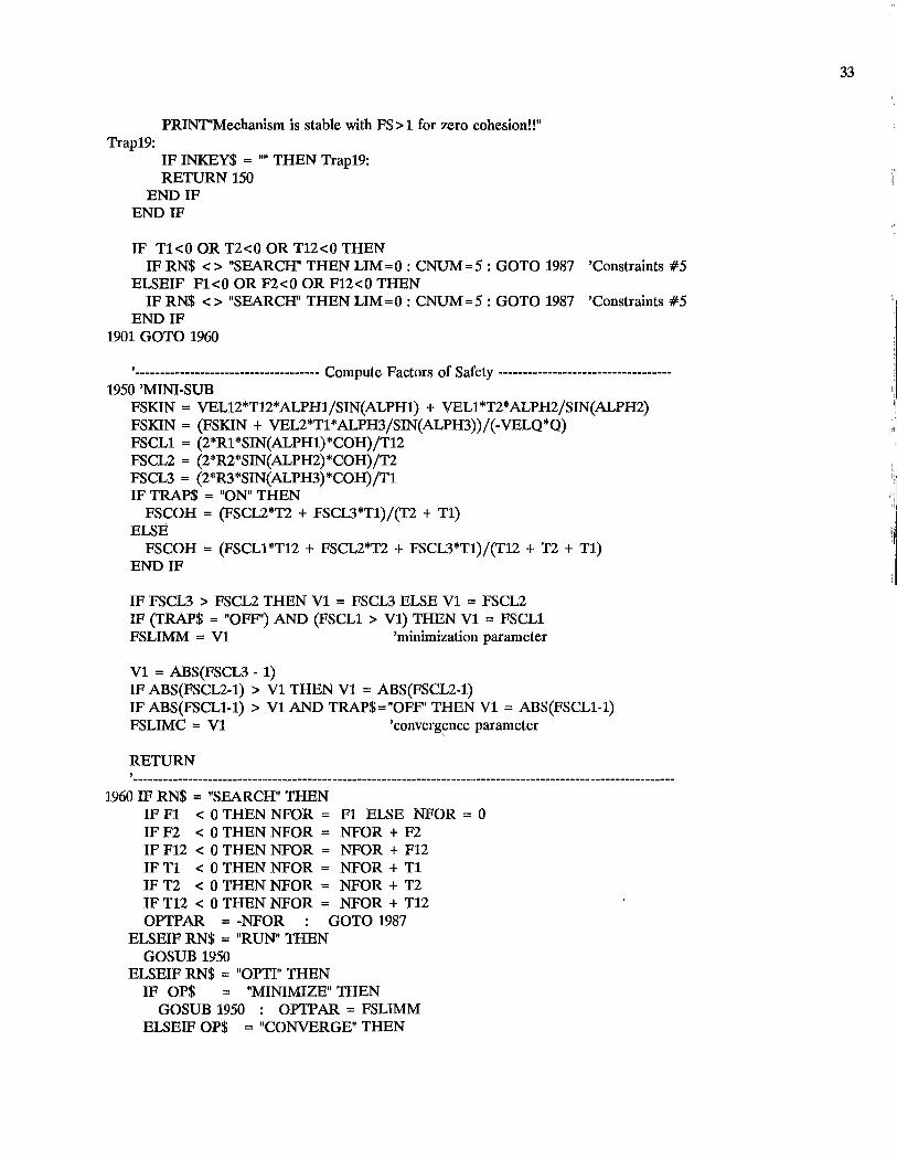
PRINT"Mechanism is stable with FS > 1 for zero cohesion!!" Trap19:

IF INKEY$ = 'III THEN Trap19: RETURN 150

END IF END IF

IF T1<0 OR T2<0 OR T12<0 THEN IF RN$ < > "SEARCH" THEN LIM=O : CNUM=5 : GOTO 1987 'Constraints #5

ELSEIF F1<0 OR F2<0 OR F12<0 THEN IF RN$ < > "SEARCH" THEN LIM=O : CNUM=5 : GOTO 1987 'Constraints #5

END IF 1901 GOTO 1960

,------------------------------------- Compute Factors of Safety -----------------------------------1950 'MINI-SUB

FSKIN = VELl2*T12*ALPH1/SIN(ALPH1) + VELl*T2*ALPH2/SIN(ALPH2) FSKIN = (FSKIN + VEL2*T1*ALPH3/SIN(ALPH3»/(-VELQ*Q) FSCL1 = (2*R1*SIN(ALPH1)*COH)/T12 FSCL2 = (2*R2*SIN(ALPH2)*COH)/T2 FSCL3 = (2*R3*SIN(ALPH3)*COH)/T1 IF TRAP$ = "ON" THEN

FSCOH = (FSCL2*T2 + FSCL3*T1)/(T2 + T1) ELSE

FSCOH = (FSCLl *T12 + FSCL2*T2 + FSCL3*T1)/(T12 + T2 + T1) END IF

IF FSCL3 > FSCL2 THEN V1 = FSCL3 ELSE V1 = FSCL2 IF (TRAP$ = "OFF') AND (FSCL1 > V1) THEN V1 = FSCL1 FSLIMM = V1 'minimization parameter

V1 = ABS(FSCL3 - 1) IF ABS(FSCL2-1) > V1 THEN V1 = ABS(FSCL2-1) IF ABS(FSCLl-1) > V1 AND TRAP$="OFF' THEN V1 = ABS(FSCL1-1) FSLIMC = V1 'converg~nce parameter

RETURN ,------------ .. ------------... ------------------------------------------------_ ... _--------------- .. -----------_ ... -_ ..

1960 IF RN$ = "SEARCH" THEN IF F1 < 0 THEN NFOR = F1 ELSE NFOR = 0 IF F2 < 0 THEN NFOR = NFOR + F2 IF F12 < 0 THEN NFOR = NFOR + F12 IF T1 < 0 THEN NFOR = NFOR + T1 IF T2 < 0 THEN NFOR = NFOR + T2 IF T12 < 0 THEN NFOR = NFOR + T12 OPTPAR = -NFOR GOTO 1987

ELSEIF RN$ = "RUN" THEN GOSUB 1950

ELSEIF RN$ = "OPTI" THEN IF OP$ = "MINIMIZE" THEN

GOSUB 1950 : OPTP AR = FSLIMM ELSEIF OP$ = "CONVERGE" THEN

33

I' l r :,1 .:11

34

GOSUB 1950 : OPTP AR = FSLIMC ELSEIF OP$ = "CONY1" THEN

GOSUB 1950 : OPTP AR = FSLIMC OPT1 = OPTP AR ELSEIF OP$ = "COHESION" THEN

GOSUB 1950 : COH = COH/FSCOH GOSUB 1950 : OPTPAR = FSLIMM : OPT1 = OPTPAR

ELSE PRINT flOPS VARIABLE = 1" : STOP

END IF END IF

1987 KEY(l) OFF IF RN$="OPTI" THEN LOCATE 12,25 PRINT RNNUM RETURN

,*********************************************************************************************************

2000 'Subroutine OPTIMIZE DELTA = 1 OP$ = "MINIMIZE" RNNUM=O : UPDATE = 0 : NUMPR=O : GOSUB 1000 GOSUB1000 IF LIM=O THEN PRINT"NON-ADMISSIBLE STARTING POINT" : RETURN OPT1 = OPTP AR : OPT2 = OPTP AR : GOSUB 8200 : GOSUB 5100

OP$ = "COHESION" : GOSUB 1000 : OP$ = "MINIMIZE" 2030 UPDATE = 0: IF KINMAT=l THEN 2034 2031 GOSUB 2470

GOSUB 2480 GOSUB 2490 : IF UPDATE = 1 THEN UPDATE=O : GOTO 2031

2034 UPDATE = 0: GOSUB 2500 GOSUB 2600 : IF UPDATE = 1 THEN UPDATE = 0 : GOTO 2030 UPDATE = 0: GOSUB 2700 GOSUB 2800: IF UPDATE = 1 THEN UPDATE =0 : GOTO 2030

IF OP$ = "MINIMIZE" THEN OP$ = "CONY1" : GOSUB 1000 OP$ = "CONVERGE"

ELSEIF OP$ = "CONVERGE" THEN OP$ = "COHESION" : GOSUB 1000 OP$ = "MINIMIZE"

ELSE PRINT "OP$ variable = 1" : STOP

END IF

GOSUB 5100 'PARTIAL PRT] IF OP$ = "MINIMIZE" THEN DELTA = DELTA/2 IF DELTA> (.0001/2) THEN 2030 , BEEP:BEEP LOCATE 5,60 : PRINT" Done LOCATE 23,10 : PRINT"Hit any Key to Return"

2170 IF INKEY$ = "" THEN 2170 RETURN '[return]

'[OPTI-COH]

'[OPTI-Q1] '[OPTI-Q2] '[OPTI-Q3] '[OPTI-Glx] '[OPTI-C2x] '[OPTI-C1y] '[OPTI-C2y]

'*********************************************************************************************************

I i

I 2200 'Subroutine SEARCH RNNVM=O : UPDATE = 0 : DELTA = 1 : NUMPR=O : GOSUB 1000 IF LIM=O THEN PRINT"NON-ADMISSIBLE STARTING POINT" IF LIM = 0 THEN PRINT"Constraint # = ";CNUM RETURN OPT1 = OPTPAR : OPT2 = OPTPAR

2230 IF NFOR = 0 THEN PRINT"ADMISSIBLE POINT FOUND" GOSUB 2470 IF UPDATE = 1 THEN UPDATE=O: GOTO 2230 GOSUB 2480 IF UPDATE = 1 THEN UPDATE=O : GOTO 2230 GOSUB 2490 IF UPDATE = 1 THEN UPDATE = 0 : GOTO 2230 GOSUB 2500 IF UPDATE = 1 THEN UPDATE=O : GOTO 2230 GOSUB 2600 IF UPDATE = 1 THEN UPDATE=O : GOTO 2230 GOSUB 2700 IF UPDATE = 1 THEN UPDATE = 0 : GOTO 2230 GOSUB 2800 IF UPDATE = 1 THEN UPDATE=O : GOTO 2230

RETURN '[OPTI-Q1]

'[OPTI-Q2]

'[OPTI-Q3]

'[OPTI-Clx]

'[OPTI-C2x]

'[OPTI-C1y]

'[OPTI-C2y]

PRINT"NFOR=";NFOR;" RNNVM=";RNNVM;" DELTA = ";DELTA DELTA = DELTA/2 : IF DELTA> (.001/2) THEN 2230 ,

BEEP : BEEP : PRINT"NOT FOUND" : RETURN '[return]

35

'******************************************************************************************************

2400 'Subroutine OPTI-A3 UPDATE=O

2410 A3X = A3X + DELTA : GOSUB 1000 IF (LIM = 1) AND (OPTPAR<OPT2) THEN

OPT2=OPTPAR : UPDATE = 1 : GOTO 2410 END IF A3X = A3X DELTA IF UPDATE = 1 THEN RETURN

2460 A3X = A3X - DELTA GOSUB 1000 IF (LIM = 1) AND (OPTPAR<OPT2) THEN

OPT2=OPTPAR : UPDATE = 1 : GOTO 2460 END IF A3X = A3X + DELTA : RETURN

'Forward Try

'Backward Try

,*****************************************************************************************************

2470 'Subroutine OPTI-Q1 OPT2=OPT1 DALPH1 = DALPH1 + 5*DELTA * (PI/180) IF (OPT2<OPT1) THEN OPT1=OPT2

DALPH1 = DALPH1 -10*DELTA * (PI/180) IF (OPT2<OPT1) THEN OPT1=OPT2

GOSUB24OO UPDATE = 1

GOSUB 2400 UPDATE = 1

'Forward Try RETURN

'Backward Try RETURN

,

,,;~ .. 1

!'I !I

:!I I

I'I :,;.i Iii

ii"

II! '

36

5*DELTA *(PI/ISO) RETURN 'Set back

'***************************************************************************************************** 2480 'Subroutine OPTI-02

OPT2=OPTI DALPH2 = DALPH2 + 5*DELTA * (PI/180) IF (OPT2<OPTI) THEN OPTI=OPT2

DALPH2 = DALPH2 -10*DELTA*(PI/180) IF (OPT2<OPTI) THEN OPTI=OPT2

DALPH2 = DALPH2 + 5*DELTA * (PI/180)

GOSUB 2400 UPDATE = 1

GOSUB 2400 UPDATE = 1

RETURN

'Forward Try RETURN

'Backward Try RETURN

'Set back

'*****************************************************************************************************

2490 'Subroutine OPTI-03 OPT2=OPTI DALPH3 = DALPH3 + 5*DELTA * (PI/180) IF (OPT2<OPTI) THEN OPTI=OPT2

DALPH3 = DALPH3 -1O*DELTA*(PI/180) IF (OPT2<OPTI) THEN OPTI=OPT2

DALPH3 = DALPH3 + 5*DELTA * (PI/180)

GOSUB 2400 UPDATE = 1

GOSUB 2400 UPDATE = 1

RETURN

'Forward Try RETURN

'Backward Try RETURN

'Set back

'*****************************************************************************************************

2500 'Subroutine OPTI-C1x OPT2=OPTI ClX = ClX + DELTA : GOSUB 2400 IF (OPT2<OPTI) THEN OPTI=OPT2

ClX = ClX - 2*DELTA : GOSUB 2400 IF (OPT2<OPTI) THEN OPTI=OPT2

ClX = ClX + DELTA : RETURN

'Forward Try UPDATE=I: RETURN

'Backward Try UPDATE=I: RETURN

'Set back to initial

,*****************************************************************************************************

2600 'Subroutine OPTI-C2x OPT2=OPTI C2X = C2X + DELTA IF (OPT2<OPTl) THEN

: GOSUB 2400 OPTI=OPT2

C2X = C2X - 2*DELTA : GOSUB 2400 IF (OPT2<OPTl) THEN OPTI=OPT2

C2X = C2X + DELTA : UPDATE=O

UPDATE=I : 'Forward Try

RETURN

'Backward Try UPDATE=I: RETURN

RETURN 'Set back to initial

'*****************************************************************************************************

--r­I

I

I

I I

2700 'Subroutine OPTI-Cly OPT2=OPTl CIY = CIY+DELTA : GOSUB 2400 IF (0PT2<OPT1) THEN OPT1=OPT2: UPDATE=l

CIY = CIY - 2*DELTA : GOSUB 2400 IF (OPT2<OPT1) THEN OPT1=OPTI: UPDATE=l

CIY = CIY + DELTA : RETURN

'FOlward Try RETURN

'Backward Try RETURN

'Set back to initial

37

'*****************************************************************************************************

2800 'Subroutine OPTI-C2y OPT2=OPTl C2Y = C2Y + DELTA : GOSUB 2400 IF (0PT2<OPT1) THEN OPT1=OPT2: UPDATE=l

'Forward Try RETURN

C2Y = C2Y - 2*DELTA : GOSUB 2400 IF (OPT2<OPT1) THEN OPT1=OPT2: UPDATE=l

'Backward Try RETURN

C2Y = C2Y + DELTA : UPDATE=O: RETURN 'Set back to initial

'*****************************************************************************************************

3000 'Subroutine ANGLE360 - calculates angle w.r.t. 360 degrees , Input - [ptl,pt2] Output - [psi] RISE=PTIY-PT2Y : HOR=PTlX-PT2X IF HOR = 0 AND RISE > 0 THEN PSI = PI/2 RETURN IF HOR = 0 AND RISE < 0 THEN PSI = 3*PI/2: RETURN PSI=ATN(ABS(RISE/HOR» IF RISE> 0 THEN

IF HOR>O THEN PSI=PSI ELSE PSI=PI-PSI ELSE

IF HOR>O THEN PSI = 2*PI-PSI ELSE PSI=PI + PSI END IF RETURN

,*****************************************************************************************************

3100 'Subroutine DISTANCE 'Input - ORTHO - 0 if dist to line; 1 if dist to othogonalline

(XO,YO)-the point (Xl,Yl)-pt. that line passes through (X2,Y2)-2nd point on line or orthogonal line

'Output - DIST, (X,Y) IF ORTHO=O THEN

M=(Y2-Yl)/(X2-Xl) : B=YI-M*Xl X=«B-YO)*(YI-Y2) + XO*(X2-Xl»/(M*(Y2-Yl) + X2 - Xl) Y=M*X + B : DIST=SQR«X-XO)"2 + (Y-YO)"2)

ELSE M=(XI-X2)/(Y2-Yl) : B=YI-M*Xl X=«B-YO)*(YI-B) - XO*Xl)/(M*(B-Yl) - Xl)

i II ,!

Iii'

Ii ;:

i: '­,. "

38

Y=M*X + B : DIST=SQR«X-XO)"2 + (Y-YO)"2) END IF RETURN

,*****************************************************************************************************

3200 'Subroutine TRIANGLE 'Input - POINTS (Xl,Yl) (X2,Y2) (X3,Y3) 'Output - area, center or gravity DX(l) = ABS(X2-Xl) : DX(2) = ABS(X3-X2) DY(l) = ABS(Y2-Yl) : DY(2) = ABS(Y3-Y2)

DXMAX = 0 : DYMAX = 0 : TEMP = 0 FOR 1= 1 TO 3

IF DX(I) > DXMAX THEN DXMAX = DX(I) IF DY(I) > DYMAX THEN DYMAX = DY(I) TEMP = TEMP + DX(I)*DY(I)

NEXT I

DX(3) = ABS(Xl-X3) DY(3) = ABS(Yl-Y3)

AREA = DXMAX*DYMAX - TEMP 12 ~=~+X2+~p:~=~+n+~p RETURN

,*****************************************************************************************************

3300 'subroutine ARC - calculates area & centroid of circular arcs 'input: [Pl,P2,P3,R] output: [A,GX,GY,THETA,ALPHA] Vl=SQR«PlX-P2X)"2 + (P1Y-P2Y)"2) IF (Vl/2)/R = > 1 THEN LIM=O GOTO 1987 'precission constraint ALPHA=(Vl/2)/R : ALPHA=ATN(ALPHA/SQR(l-ALPHA"2» '[arcsin] PTlX=PlX: PT1Y=P1Y : PTIX=P2X : PT2Y=P2Y GOSUB 3000 THETA = PSI , [ANGLE360] V3=(2/3)*R*SIN(ALPHA)"3/(ALPHA-SIN(ALPHA)*COS(ALPHA» A=R"2*(ALPHA-SIN(2*ALPHA)/2) PTlX=(PlX+P2X)/2: PT1Y=(P1Y+P2Y)/2: PT2X=P3X: PT2Y=P3Y GOSUB 3000 '[ angle360] GX = P3X + ABS(V3*SIN(THETA»*SGN(COS(PSI» GY = P3Y + ABS(V3*COS(THETA»*SGN(SIN(PSI» RETURN

,*****************************************************************************************************

3400 ' subroutine ETA - calculate angle eta , Input: [theta,R,(Cx,Cy),alpha,Gx] Output: [eta,K,Q,QP] RT = R*ALPHA/SIN(ALPHA) RPHI = R*SIN(PHI) : IF PHI=O THEN RPHI=lE-09 KX = CX + ABS(RT*SIN(THETA»*SGN(COS(PTHETA» KY = CY + ABS(RT*COS(THETA»*SGN(SIN(PTHETA»

TEMP = R *(ALPHA/SIN(ALPHA»*TAN(DALPHA) QX = KX + TEMP*COS(THETA) : QY = KY + TEMP*SIN(THETA) B = SQR«CX-QX)"2 + (CY-QY)"2)

r

I

OMEGA = ATN(SQR(1-(RPHI/B)"2)/(RPHI/B» 'arccos(R/B) IF QX=CX THEN OMEGB=PI/2: GOTO 3410 OMEGB = ATN«CY-QY)/(QX-CX» : IF QX<CX THEN OMEGB = PI+OMEGB

3410 SELECT CASE OPTN CASE 1

QPX=CX-RPHI*COS(PI-OMEGB-OMEGA) : QPY = CY-RPHI*SIN(PI-OMEGB-OMEGA) CASE 2

QPX = CX+RPHI*COS(OMEGB-OMEGA): QPY = CY-RPHI*SIN(OMEGB-OMEGA) CASE 3

QPX = CX+RPHI*COS(OMEGB-OMEGA): QPY = CY-RPHI*SIN(OMEGB-OMEGA) END SELECT

PT1X=QPX : PT1Y=QPY : PT2X=QX : PT2Y=QY GOSUB 3000 : ETA = PSI RETURN

'[ANGLE360]

39

,*****************************************************************************************************

3500 'Subroutine CLOCKWISE 'Input: (CPTx,CPTy) - center pt. , (VFx, VFy) - vector front

(VRx, VRy) - vector rear 'output: CLCK$ = "CLCK wise" or "CNTR clockwise"

IF VFY = VRY THEN IF (VFY-CPTY) > (VRY-CPTY) THEN CLCK$="CNTR" ELSE CLCK$="CLCK" RETURN

END IF IF VFX= VRX THEN

B = VFX ELSE

M = (VFY-VRY)/(VFX-VRX) : B = VFX - (VFY-CPTY)/M END IF IF (B-CPTX) > 0 AND SGN(VFY-CPTY) < > SGN(VRY-CPTY) THEN

IF (VFY-CPTY) > (VRY-CPTy) THEN CLCK$="CNTR" ELSE CLCK$="CLCK" RETURN

ELSE PT2X=CPTX: PT2Y=CPTY: PT1X=VFX: PTIY=VFY: GOSUB 3000: OMEGF=PSI PT1X=VRX: PT1Y=VRY: GOSUB 3000: OMEGR=PSI IF (OMEGR - OMEGF) > 0 THEN CLCK$="CLCK" ELSE CLCK$="CNTR" RETURN

END IF ,-------------------------------------------------------------------------------------------------------------------------------------------.. --

3501 'Subroutine CLOCKWISE - 2nd Option 'Input: (CPTx,CPTy) - center pt. , (VRx,VRy) ; OMEGA - vector point & orientation 'output: CLCK$ = "CLCK wise" or "CNTR clockwise"

IF OMEGA = 0 THEN IF (CPTy > VRy) THEN CLCK$= "CNTR" ELSE CLCK$="CLCK" RETURN

ELSEIF OMEGA = PI THEN

j.; 40

IF (CPTy < VRy) THEN CLCK$="CNTR" ELSE CLCK$="CLCK" RETURN

END IF IF OMEGA = > PI THEN OMEGA = OMEGA - 2*PI IF OMEGA = PI/2 THEN

IF (CPTx < VRx) THEN CLCK$="CNTR" ELSE CLCK$="CLCK" RETURN

ELSEIF OMEGA = -PI/2 THEN IF (CPTx > VRx) THEN CLCK$= "CNTR" ELSE CLCK$="CLCK" RETURN

END IF

M = TAN(OMEGA) : B = VRy - M*VRx IF ABS(OMEGA) < PIj2 THEN

IF (CPTy > CPTX*M + B) THEN CLCK$="CNTR" ELSE CLCK$="CLCK" ELSE

IF (CPTy < CPTX*M + B) THEN CLCK$="CNTR" ELSE CLCK$="CLCK" END IF RETURN

,*****************************************************************************************************

3600 'Subroutine HODOGRAPH 'INPUT: MECH, PI, THETl-2-3, ALPHl-2-3, Cl & C3 'LOCAL: ANGLES: LIN-MI-M2-M3-BI-D2-A3

POINTS: ClxHD, M2xHD, M3xHD, B2xHD, B3xHD,D2xHD,A3xHD 'OUTPUT: VEL-0-1-2-12 , .. _ .. _----_ .. _ ... ------_ .. _--_ ..... _---------_ ... _------ ......

'Calculate Angles: IF ClX= C3X THEN

ANGLIN = PI ELSE

ANGLIN = ATN«CIY-C3Y)/(ClX-C3X) + PI/2 END IF

SELECT CASE MECH CASE 1

ANGMI = THETI ALPHI + PI ANGBI = ANGM2 = THET2 ALPH2 + PI ANGD2 ANGM3 = THET3 + ALPH3 PI ANGA3 ANGWR ANGWR PI/2 ANGWL =

CASE 2 ANGMI = THETl ALPHl + PI ANGBl ANGM2 THET2 ALPH2 + PI ANGD2 ANGM3 THET3 ALPH3 PI ANGA3 ANGWR = ANGWR PI/2 ANGWL =

CASE 3 ANGMI = THETl + ALPHI + PI ANGBl ANGM2 = THET2 + ALPH2 + PI ANGD2 ANGM3 THET3 + ALPH3 PI ANGA3 = ANGWR ANGWR + PI/2 ANGWL =

THETI + THET2 + THET3 ANGWL

THETl + THET2 + THET3 + ANGWL +

THETl THET2 THET3 ANGWL

ALPHl + PI ALPH2 + PI ALPH3 PI PI/2

ALPHl + PI ALPH2 + PI ALPH3 PI PI/2

ALPHl + PI ALPH2 + PI ALPH3 PI PI/2

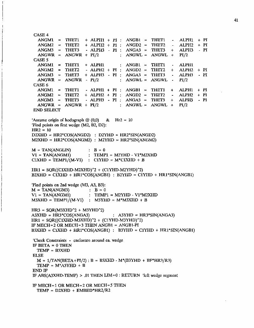
r I I I

j I I

CASE 4 ANGMl THETl + ALPHl + PI ANGBl = THETl ANGM2 THET2 + ALPH2 + PI ANGD2 = THET2 ANGM3 THET3 ALPH3 PI ANGA3 = THET3 + ANGWR ANGWR + PI/2 ANGWL = ANGWL +

CASES ANGMl THETl + ALPHl ANGBl = THETl ANGM2 THET2 ALPH2 + PI ANGD2 = THET2 + ANGM3 = THET3 + ALPH3 PI ANGA3 = THET3 ANGWR = ANGWR - PI/2 ANGWL = ANGWL

CASE 6 ANGMl THETl ALPHl + PI ANGBl = THETl + ANGM2 THET2 + ALPH2 + PI ANGD2 = THET2 ANGM3 THET3 - ALPH3 PI ANGA3 = THET3 + ANGWR ANGWR + PI/2 ANGWL = ANGWL +

END SELECT

'Assume origin of hodograph @ (0,0) & Hr2 = 10 'Find points on first wedge (M2, B2, D2): HR2 = 10 D2XHD = HR2*COS(ANGD2) : D2YHD = HR2*SIN(ANGD2) M2XHD = HR2*COS(ANGM2) : M2YHD = HR2*SIN(ANGM2)

M = TAN(ANGLIN) Vl = TAN(ANGM1) ClXHD = TEMP1/(M-Vl)

B=O : TEMPl = M2YHD - Vl *M2XHD : C1YHD = M*ClXHD + B

HRl = SQR«ClXHD-M2XHD)"2 + (C1YHD-M2YHD)"2)

ALPHl ALPH2 ALPH3 PI/2

ALPHl ALPH2 ALPH3 PI/2

ALPHl ALPH2 ALPH3 PI/2

B2XHD = ClXHD + HRl *COS(ANGB1) : B2YHD = C1YHD + HRl *SIN(ANGB1)

'Find points on 2nd wedge (M3, A3, B3): M = TAN(ANGM3) B = 0 Vl = TAN(ANGM1) : TEMPl = M2YHD - Vl *M2XHD M3XHD = TEMP1/(M-Vl) : M3YHD = M*M3XHD + B

HR3 = SQR(M3XHD"2 + M3YHD"2) A3XHD = HR3*COS(ANGA3) : A3YHD = HR3*SIN(ANGA3) HRl = SQR«ClXHD-M3XHD)"2 + (C1YHD-M3YHD)"2) IF MECH=2 OR MECH=3 THEN ANGBl = ANGB1-PI B3XHD = ClXHD + HR1*COS(ANGB1) : B3YHD = C1YHD + HR1*SIN(ANGB1)

'Check Constraints - enclosure around ea. wedge IF BETA = 0 THEN

TEMP = B3XHD ELSE

M = 1/TAN(BETA+PI/2) : B = B3XHD - M*(B3YHD + BF*HR3/R3) TEMP = M* A3YHD + B

END IF IF ABS(A3XHD-TEMP) > .01 THEN LIM = 0 : RETURN 'left wedge segment

IF MECH=l OR MECH=2 OR MECH=5 THEN TEMP = D2XHD + EMBED*HR2/R2

41

+ PI + PI

PI

+ PI PI

+ PI + PI

PI

Ii I!

1

1'1 j!

'Iii [ ,

II 1>1 Ii I

42

ELSE TEMP == D2XHD - EMBED*HR2/R2

END IF IF ABS(B2XHD-TEMP) > .01 THEN LIM=O: RETURN 'right wedge segment

VELQ = (B2YHD + D2YHD)/2 + E*(D2YHD - B2YHD)/(B2X - BlX) VELl = SQR(M2XHD"2 + M2YHD"'2) : VEL2 = SQR(M3XHD"2 + M3YHD"2) VELIZ = SQR«M3XHD-M2XHD)"2 + (M3YHD-M2YHD)"2) VELWR == RWR*(HR2/R2)*SIN(ANGWR) : VELWL = RWL*(HR3/R3)*SIN(ANGWL)

RETURN

'*****************************************************************************************************

3700 'Subroutine MATRIX - gauss elimination by pivot points 'MAT(i,j) - square matrix of coefficients 'B(i) - vector of constants on right side of equations 'X(i) - solution vector ( [MAT]{X} = {B} ) ,-----------------_ .. _------------------------------------... --------

N=6 FOR 1=1 TO N; MAT(7,1)=B(I) : NEXT I

FOR PVR = 1 TO N PPT = MAT(PVR,PVR) FOR I = 1 TO (N + 1) : MAT(I,PVR) = MAT(I,PVR)/PPT : NEXT I PPT = MAT(PVR,PVR) FORJ = 1 TO N

IF J = PVR THEN 3710 ELIM = MA T(PVR,J) FOR I = 1 TO (N+l)

MAT(I,J) = PPT*MAT(I,J) - ELIM*MAT(I,PVR) NEXT I

3710 'ENDIF NEXTJ

NEXTPVR RETURN

,**********************************************************************************************************

4000 'Subroutine INTERACTIVE INPUT KEY OFF : CLS : GOSUB 6000 : ROW = 1 GOSUB 8100 '[input screen setup] KEY(l1) ON ON KEY(l1) GOSUB 4020 KEY(14) ON ON KEY(14) GOSUB 4030

COLOR 14,0 : FOR ROW = 2 TO 18

: 1=0 : DOT=O

'cursor up 'cursor down

LOCATE LY(ROW),LX(ROW): PRINT USING"####.#### ";VAR(ROW) NEXT ROW : ROW = 1 : COLOR 0,7 LOCATE LY(ROW),LX(ROW): PRINT USING"####.#### ";VAR(ROW) COLOR 7,0

4010 V$ = INKEY$ : IF V$ = "" THEN 4010 RST$ = "Y" : OOTO 4060 , -----------_ .. ------------------------------------------------------------------------------------.---------------....... -------------------------------

r

I I , I 'mini-Subroutine KEYOPTION

4020 LOCATE LY(ROW),LX(ROW) IF ROW = 19 THEN PRINT"RETURN" IF ROW < 19 THEN PRINT USING"####.#### IF ROW <> 1 THEN ROW = ROW-l RST$ == "Y" : RETURN 4040

'cursor up

";VAR(ROW)

4030 IF ROW=19 THEN RETURN 4040 'cursor down LOCATE LY(ROW),LX(ROW): PRINT USING"####.#### ";VAR(ROW) ROW = ROW + 1 : RST$= "Y" : RETURN 4040 ,

43

------------_ ... _--------------------------------------------------------------------------------------------------... ------------- ..... -"! .. __ .. - .... --------...

4040 COLOR 0,7 : LOCATE LY(ROW),LX(ROW) IF ROW < 19 THEN PRINT USING"####.#### IF ROW = 19 THEN PRINT" RETURN "; COLOR 7,0

4050 V$ = INKEY$ : IF V$ = '"' THEN 4050 4060 IF LEN(V$)=2 THEN V$ = RIGHT$(V$,l)

IF ASC(V$) < > 13 THEN

";VAR(ROW)

IF RST$="Y" THEN VAR(ROW) = lE-30 : DOT=O RST$="N": NEGA=l CHCK$ = "NUM" IF ASC(V$) < 45 THEN CHCK$ = "LET" : BEEP IF ASC(V$) > 57 THEN CHCK$ = "LET" : BEEP IF ASC(V$) = 47 THEN CHCK$ = "LET" : BEEP IF ASC(V$) = 46 THEN CHCK$ = "DOT": DOT = DOT + 1 IF ASC(V$) = 45 THEN CHCK$ = "MIN" : NEGA = -NEGA

IF DOT=O AND CHCK$="NUM" THEN VAR(ROW) = VAR(ROW)*lO + NEGA*VAL(V$) IF DOT=l AND CHCK$="DOT" THEN I = 0 IF DOT>O AND CHCK$="NUM" THEN 1=1-1: VAR(ROW)=VAR(ROW)+NEGA*VAL(V$)*10AI IF DOT>l AND CHCK$="DOT" THEN BEEP IF CHCK$ = "MIN" THEN V AR(ROW) = -VAR(ROW) GOTO 4040

END IF

IF ROW=19 THEN KEY(l1) OFF: KEY(14) OFF

FOR I = 1 TO 15 IF ABS(VAR(I» < lE-20 THEN VAR(I) = FIX(VAR(I»

NEXT I GOSUB 6100 : RETURN

END IF LOCATE LY(ROW),LX(ROW) : PRINT USING"####.#### RST$="Y" : ROW = ROW + 1 GOTO 4040

";VAR(ROW)

,*****************************************************************************************************

4100 'Subroutine FILE INPUT COLOR 0,7,1 : LOCATE 23,10 : INPUT" d:fname.ext = "; F$ COLOR 7,0 : LOCATE 23,10: PRINT" OPEN F$ FOR INPUT AS #1

'1 :i

, , : ~

44

INPUT #1, GAMA, COH, PHI, FSPHI INPUT #1, BETA, BF, BW INPUT #1, Q, E, EMBED INPUT #1, ClX, Cl Y, C2X, C2Y INPUT #1, A3X,MECH INPUT #1, DALPHl,DALPH2,DALPH3 CLOSE #1

PHI = PHI*(PI/180) BETA = BETA *(PI/180) IF GAMA=O THEN GAMA = IE-3D

RETURN

,*****************************************************************************************************

4200 'Subroutine fIle OUTput PHI = PHI*(180/PI) BETA = BETA*(180/PI)

OPEN "OPTIC.LOG" FOR OUTPUT AS #2 WRITE #2, GAMA, COH, PHI, FSPHI WRITE #2, BETA, BF, BW WRITE #2, Q, E, EMBED WRITE #2, ClX, CIY, C2X, C2Y WRITE #2, A3X,MECH WRITE #2, DALPHl,DALPH2,DALPH3 CLOSE #2

PHI=PHI*(PI/180) BETA = BETA*(PI/180) RETURN

,********************************************************************************************************* 5000 'Subroutine PRINT

CLS LOCATE 3,20 : PRINT"NUMBER OF INTERATIONS = ";RNNVM LOCATE 4,10 : PRINT"Mechanism #";MECH LOCATE 4,40 : PRINT DATE$,TIME$ LOCATE 5,5 : PRINT

I FOR 1=6 TO 15

LOCATE 1,5 : PRINT" I" LOCATE 1,75 PRINT" I" NEXT I LOCATE 15,5 : PRINT

"I~--------------------------------------------------------------------------__ --JI"

LOCATE 17,1 : PRINT "Geometry:" PRINT"Circle # ------ (CX,CY) -------- R ---- ALPHA --- THETA -- ETA--" PRINT" 1 ("; PRINT USING"####.###,";ClX; PRINT USING"##.###) ";CIY; PRINT USING" ###.### ";Rl;ALPHl *(180/PI);THETl *(180/PI);ETAl * (180/PI) PRINT" 2 ("; PRINT USING"###.###,";C2X; PRINT USING"##.###) ";C2Y; PRINT USING" ###.### ";R2;ALPH2*(180/PI);THET2*(180/PI);ETA2*(180/PI) PRINT" 3 ("; PRINT USING"###.###,"jC3X; PRINT USING"##.###) ";C3Y;

r I ! I !

PRINT USING" ###.### ";R3;ALPH3*(180/PI);THET3*(180/PI);ETA3*(180/PI)

LOCATE 6,10 LOCATE 7,16 LOCATE 7,46 LOCATE 7,58 LOCATE 8,16 LOCATE 10,8 LOCATE 10,45 LOCATE 11,8 LOCATE 11,35 LOCATE 12,8 LOCATE 12,40 LOCATE 14,10 LOCATE 14,49

: PRINT "Factors of Safety: " : PRINT USING"Limiting Cohesion = ##.####";FSCLl : PRINT USING"##.####";FSCL2 : PRINT USING"##.####";FSCL3 : PRINT USING"Kinetic Cohesion = ##.####";FSKIN : PRINT "Footing Load,Eccentricity & Embedment = " : PRINT USING"######.###";O;E;EMBED : PRINT "Slope Angle = " : PRINT USING"###.###, ";BETA*(180/PI) : PRINT"Width, & Distance from Crest = " : PRINT USING"######.###";BW,BF : PRINT "Soil Weight, cohesion, & Friction Angle = " : PRINT USING"####.##,";GAMA;COH;PHI*(180/PI)

COLOR 29: LOCATE 24,50: PRINT"Press any key to continue": COLOR 2,0 TrapA:

IF INKEY$="" THEN TrapA: CLS PRINT "Summary of Areas & Weights:" PRINr "Region # --- Area ----- (Center of Gravity) ------ weight -----" H$(l) = "ARC 1 " : H$(2) = "ARC 2 ": H$(3) = "ARC 3 " H$( 4) = "Rt Triag" : H$(5) = "Lt Poly" H$(6)="Rt Wedge" : H$(7)="Lt Wedge" A(6)=AR : GX(6)= GRX : GY(6)=GRY: A(7)=AL: GX(7)=GLX : GY(7)=GLY FOR 1=1 TO 7

PRINT H$(I); PRINT USING"###.### (";A(I); PRINT USING"###.###,";GX(I); : PRINT USING"###.###)";GY(I); PRINT USING" ####.##";A(I)*GAMA

NEXT I

PRINT "summary of forces and force geometry:" PRINT"Circle # -- force # -- Friction Force --- Cohesion Force -------" PRINT" 1 12 "; PRINT USING" ####.###"; F12;T12 PRINT" 2 PRINT USING" PRINT" 3 PRINT USING"

2 "; ####.###"; F2;T2

1 "; ####.###"; Fl;Tl

PRINT "Circle # ------- pt K ---------- pt 0 -------------- pt OP ----" PRINT" 1 "; PRINT USING"(###.###,"; K1X; : PRINT USING"###.###) "; K1Y; PRINT USING"(###.###,"; 01X; : PRINT USING"###.###) "; 01Y; PRINT USING"(###.###,"; OP1X;: PRINT USING"###.###)"; OP1Y PRINT" 2 "; PRINT USING"(###.###,"; K2X; : PRINT USING"###.###) "; K2Y; PRINT USING"(###.###,"; 02X; : PRINT USING"###.###) "; 02Y; PRINT USING"(###.###,"; OP2X;: PRINT USING"###.###)"; OP2Y PRINT" 3 ";

45

I

I I' :!

'!I'

!i "

, , , ,

46

PRINT USING"(###.###,"; K3X; : PRINT USING"###.###) "; K3Y; PRINT USING"(###.###,"; Q3Xj : PRINT USING"###.###) "; Q3Y; PRINT USING"(###.###,"; QP3X;: PRINT USING"###.###)"; QP3Y

PRINT USING"point A3 = (###.###"; A3Xj : PRINT USING",###.###)"j A3Y PRINT USING"point M = (###.###"; MX; : PRINT USING",###.###)"; MY PRINT ARMRF,ARMRT,ARMLF,ARMLT

TrapB: IF INKEY$ = "" THEN TrapB: CLS : LOCATE 1,15: PRINT"------ HODOGRAPH DATA: ------" PRINT"Circle # 1 2 3" PRINT"Center Pt." : PRINT"Point B" PRINT"Angle M" : PRINT"Angle A"

PRINT"Point M" PRINT"Point D": PRINT"Point A" PRINT"Angle B": PRINT"Angle D"

LOCATE 3,12 PRINT USING"###.###,";ClXHD; : PRINT USING"###.###";CIYHD LOCATE 3,36 PRINT "(0,0) (0,0)" LOCATE 4,32 PRINT USING"##.###,"jM2XHD; : PRINT USING"##.###";M2YHD LOCATE 5,32 PRINT USING"##.###,"jB2XHDj : PRINT USING"##.###";B2YHD LOCATE 6,32 PRINT USING"##.###,"jD2XHD; : PRINT USING"##.###";D2YHD LOCATE 4,52 PRINT USING"##.###,";M3XHDj : PRINT USING"##.###";M3YHD LOCATE 5,52 PRINT USING"##.###,";B3XHDj : PRINT USING"##.###";B3YHD LOCATE 7,52 PRINT USING"##.###,";A3XHD; : PRINT USING"##.###";A3YHD LOCATE 8,15 PRINT USING,,####.###o";ANGMl*(180/PI); LOCATE 8,34 PRINT USING,,####.###o";ANGM2*(180/PI); LOCATE 8,54 PRINT USING,,####.###o";ANGM3*(180/PI); LOCATE 9,15 PRINT USING,,####.###o";ANGBl * (180/PI); LOCATE 10,34: PRINT USING,,####.###o";ANGD2*(180/PI); LOCATE 11,54: PRINT USING,,####.###o";ANGA3*(180/PI) PRINT USING" Angle of circle centers line = ####.###o";ANGLIN*(180/PI) PRINT"--------------------------------------------------------------------------------------------"

PRINT USING"VELQ = ##.####";VELQ PRINT USING"VELl = ##.####";VELI PRINT USING"VEL2 = ##.####";VEL2 PRINT USING"VELl2= ##.####";VEL12 PRINT USING"VELWR= ##.####";VELWR PRINT USING"VELWL= ##.####";VELWL PRINT: PRINT".,. = ";GAMA COLOR 7,0

TrapC: IF INKEY$ = t"t THEN TrapC:

IF Tl<O THEN 5010 IF T2<0 THEN 5010 IF T12<0 THEN 5010 RETURN

5010 PRINT "***Equilibrium Cohesive Force is Negative ...... " PRINT "Slope is Stable, but Factor of Safety is not Correctl ***"

TrapD: IF INKEY$ = "" THEN TrapD: RETURN

----------~==",...-

47

,***************************************************************************************************** 5100 'Subroutine PARTIAL-PRINT

NUMPR =NUMPR + 1 : IF NUMPR>4 THEN NUMPR=4 FOR 1=3 TO 1 STEP (-1)

FSC(I+1)=FSC(I) : COH(I+1)=COH(I) : DELTA(I+1) = DELTA(I) FS1(I+1)=FS1(I) : FS2(1+1)=FS2(I) : FS3(1+1) = FS3(I) : FSK(I+1) = FSK(I)

NEXT I FSC(l)=FSCOH : COH(l)=COH DELTA(l) = DELTA FS1(1) = FSCL1 : FS2(1)=FSCL2 : FS3(1)=FSCL3 : FSK(l)=FSKIN , FOR 1=1 TO NUMPR

LOCATE (1+ 15),8 LOCATE (I + 15),18 LOCATE (1+15),25 LOCATE (1+15),31 LOCATE (I + 15),40 LOCATE (1+ 15),52 LOCATE (I + 15),65

NEXT I RETURN

PRINT USING"#.####"; DELTA(I) PRINT USING"##.###"; FS1(I) PRINT USING"##.###"; FS2(I) PRINT USING"##.###"; FS3(I) PRINT USING"## .####";FSC(I) PRINT USING"##.####";FSK(I) PRINT USING"###.##"; COH(I)

,*****************************************************************************************************

6000 'Subroutine ARRAY-IN PHI = PHI * (180/PI) : BETA = BETA * (180/PI) DALPH1=DALPH1*(180/PI) : DALPH2=DALPH2*(180/PI) : DALPH3=DALPH3*(180/PI)

VAR(l) = GAMA VAR(2) = COH VAR(3) = PHI VAR(4) = BETA VAR(5) = BF VAR(6) = BW VAR(7) = Q V AR(8) = E V AR(9) = EMBED VAR(lO)= Clx VAR(l1)= Cly VAR(12)= C2x V AR(13) = C2y V AR(14) = A3x VAR(15) = MECH VAR(16) = DALPHl VAR(17) = DALPH2: VAR(18) = DALPH3

RETURN

,*****************************************************************************************************

6100 'Subroutine ARRAY-OUT GAMA = VAR(l) COH = VAR(2) PHI = VAR(3) BETA = VAR(4) BF = VAR(5) BW = VAR(6) Q = VAR(7) E = VAR(8) EMBED = ABS(VAR(9» Clx = VAR(10) Cly = VAR(l1) C2x = VAR(12) C2y = VAR(13) A3x = VAR(14) MECH = VAR(15) DALPH1 = VAR(16) DALPH2 = VAR(17) DALPH3 = VAR(18) DALPH1=DALPHl * (PI/180) : DALPH2=DALPH2*(PI/180) : DALPH3=DALPH3*(PI/180) PHI = PHI*(PI/180) : BETA = BETA * (PI/180) RETURN

,*****************************************************************************************************

6200 'Subroutine [MATRIX-IN]

I

II 'II 'I !

I I, , ) ~

48

FOR 1= 1 TO 6 FOR J=l TO 7 : MAT(J,I)=O : NEXT J B(I) = 0

NEXT I MAT(l,l)=SIN(ETA3) : MAT(2,1)=SIN(THET3) : MAT(3,1)=SIN(ETA2) MAT(1,2) = COS(ETA3) : MAT(2,2) = COS(THET3) : MAT(3,2) = COS(ETA2) MAT(4,1)=SIN(THET2) : MAT(4,2)=COS(THET2) MAT(3,3)=SIN(ETA2) MAT(4,3)=SIN(THET2) MAT(5,3)=SIN(ETA1) MAT(3,4) = COS(ETA2) : MAT( 4,4) = COS(THET2) MAT(5,4) = COS (ETA1) MAT(6,3) =SIN(THET1) : MAT(6,4) = COS(THET1) MAT(5,5)=ARMLF : MAT(6,5)=ARMLT MAT(1,6) =ARMRF : MAT(2,6) =ARMRT

IF MECH=l OR MECH=2 OR MECH=5 THEN MAT(3,6) = -R2*SIN(PHI): MAT( 4,6) = -R2*(ALPH2/SIN(ALPH2»

ELSE MAT(3,6)= R2*SIN(PHI): MAT(4,6)= R2*(ALPH2/SIN(ALPH2»

END IF B(l) = Q + WR + WL : B(3) = Q + WR B(6) = -(Q*«B1X+B2X)/2+E-C2X) + WR*(GRX-C2X) + WL*(GLX-C2X»

RETURN

,*****************************************************************************************************

6300 'Subroutine INITIALIZE FOR i=l TO 6 : A(i) =0 : Gx(i)=0 : Gy(i)=0 : NEXT i R1=0 : R2=0 : R3=0 : C3X=0 : C3Y=0 : ALPH1=0 : ALPH2=0 : ALPH3=0 THET1=0 : THET2=0 : THET3=0 : ETA1=0 : ETA2=O : ETA3=O F1=0 : F2=0 : F12=0 : T1=0 : T2=0 : T12=0 K1X=O : j(lY=O : K2X=O : K2Y=O : K3X=O : K3Y=O Q1X=O : Q1Y=0 : Q2X=0 : Q2Y=0 : Q3X=0 : Q3Y=0 QP1X=O : QP1Y=0 : QP2X=0 : QP2Y=0 : QP3X=0 : QP3Y=0 MX=O : MY=O : A3Y=O : FSCL1=O : FSCL2=0 : FSCL3=0 RNNUM=O RETURN

,*****************************************************************************************************

8000 'Subroutine MAIN MENU SCREEN SETUP , configure cursor locations LX(l)=30 : LY(l) = 4: LX(5) =30 : LY(5) =10: LX(9) = 50: LY(9) =17 LX(2)=30 : LY(2) = 5: LX(6)=30 : LY(6) =11 : LX(10)= 20 : LY(10)=18 LX(3) =30 : LY(3) = 6: LX(7) =30 : LY(7) =14: LX(11) = 50: LY(11)=18 LX(4)=30 : LY(4) = 9: LX(8)=20 : LY(8) =17: LX(12) = 30 : LY(12) =20

COLOR 13,0 : LOCATE 2,10: PRINT"----------- MAIN MENU ----------------" COLOR 14,0 'Headings LOCATE 3,10: PRINT" 1) Data Manipulation ... " LOCATE 8,10: PRINT"2) Processing .................. " LOCATE 13,10: PRINT"3) Output ........................ " LOCATE 16,10: PRINT"4) Options ....................... "

'Choices --------------- >

r

I

CH$(l)= " < Interactive input > " : CH$(2)= " < Data flle input CH$(3)= " < File save > " : CH$(4)= " < Run present config. CH$(5)= " < Optimize config. > " : CH$(6)= " < Admissible search CH$(7)= " < Print results > " : CH$(8) = " < 2 Surface solution CH$(9)= " < 3 Surface solution > " : CH$(10)= " < Kinematic solution CH$(l1)= " < Limit analysis sol. > " : CH$(12)= " < EXIT PROGRAM

COLOR 12,0 FOR ROW = 1 TO 12 LOCATE LY(ROW),LX(ROW) : PRINT CH$(ROW) NEXT ROW

COLOR 10,0 IF TRAP$= "ON" THEN

LOCATE LY(8),LX(8) PRINT CH$(8) ELSE

LOCATE LY(9),LX(9) PRINT CH$(9) END IF IF KINMAT= 1 THEN

LOCATE LY(10),LX(10) PRINT CH$(10) ELSE

LOCATE LY(l1),LX(l1) PRINT CH$(l1) END IF COLOR 0,7 RETURN

> " > " > " > " > " > "

----------~~-

49

:1 I, II

:1,

Ii

,*****************************************************************************************************

8100 'subroutine INPUT SCREEN SETUP 'Configure cursor locations LX(l) =49 : LY(l)=3 LX(6) =54 : LY(6)=10 LX(l1) =50 : LY(l1) = 17 LX(2) =49 : LY(2)=4 LX(7) =54 : LY(7) = 11 LX(12) =50 : LY(12)=18 LX(3) =49 : LY(3)=5 : LX(8)=54 : LY(8)=12 LX(13) =50 : LY(13)=19 LX(4) =54 : LY(4)=8 : LX(9)=54 : LY(9) = 13 LX(14) =50 : LY(14)=20 LX(5) =54 : LY(5)=9 : LX(1O)=50 : LY(10)=16 : LX(15) =50 : LY(15) =21 LX(16)=3O : LY(16) =22 : LX(17) =45 : LY(17) =22 LX(18)=60 : LY(18) =22 : LX(19) =30 : LY(19) =24

CLS : COLOR 2,0 LOCATE 2,20 : PRINT" Soil Parameters: LOCATE 7,20 : PRINT" Slope Geometry: LOCATE 15,20 : PRINT" Failure Mechanism: " LOCATE 24,30 : PRINT"RETURN";

COLOR 12,0 LOCATE 3,10 : PRINT"Unit Weight of Soil­LOCATE 4,10 : PRINT"Cohesion­LOCATE 5,10 : PRINT"Friction Angle -LOCATE 8,10 : PRINT"Slope Angle -LOCATE 9,10 : PRINT"Distance of Footing from Slope Crest -LOCATE 10,10 : PRINT"Width of Footing-LOCATE 11,10 : PRINT"Load on Footing (force/unit length) -LOCATE 12,10 : PRINT"Load Eccentricity-LOCATE 13,10 : PRINT"Footing Embedment depth -LOCATE 16,10 : PRINT"Center of First Circle-

T =" C =" ¢ ="

Clx ="

B =" b =" w =" Q =" e =" S ="

50

LOCATE 17,10 : PRINT" LOCATE 18,10 : PRINT"Center of Second Circle­LOCATE 19,10 : PRINT" LOCATE 20,10 : PRINT"Toe of Failure Mechanism -LOCATE 21,10 : PRINT"Mechanism configuration­LOCATE 22,10 : PRINT"da = " COLOR 7,0 RETURN

Cly =" C2x =" C2y =" A3x ="

MECH ="

,*****************************************************************************************************

8200 'Subroutine PARTIAL RESULTS SETUP CLS : COLOR 31 : LOCATE 5,60 : PRINT "Optimizing ... " : COLOR 7 LOCATE 10,20 PRINT "Partial Results" LOCATE 13,6

PRINT" rrU =============r========================r===============9==============9======= =====i1n"

LOCATE 14,6 FSc I Cohesion II"

LOCATE 15,6

PRINT" II Opt. Step FS1 FS2 FS3 Limiting FSc Kinetic

PRINT"Il=: ====+=========+======-/-=====11-== =======l:I"

LOCATE 16,6

II" LOCATE 17,6

II" LOCATE 18,6

II" LOCATE 19,6

II"

PRINT" II

PRINT" II

PRINT" II

PRINT" II

LOCATE 20,6 PRINT" I!::II ================================================ ===::::!JI! "

RETURN

,*****************************************************************************************************

9900 'Subroutine ERROR CLS PRINT PRINT"IBM BASIC 3.0 - Error Number = ";ERR IF (ERR=5) OR (ERR=6) OR (ERR = 11) THEN

PRINT"Incomplete input data has been specified or program is" PRINT"not capable of specified geometry & mechanism"

END IF Trap4:

IF INKEY$ = '''' THEN Trap4 9999 RESUME 150

,*****************************************************************************************************

INf.BU.OF MlNES,PGH.,PA 29325