Plausibly Exogenous

Tim Conley, Christian Hansen, and Peter E. Rossi∗

14 March 2006. This draft: 18 May 2007.

Abstract

Instrumental variables (IVs) are widely used to identify effects in models with po-

tentially endogenous explanatory variables. In many cases, the instrument exclusion

restriction that underlies the validity of the usual IV inference holds only approxi-

mately; that is, the instruments are ‘plausibly exogenous.’ We introduce a method of

relaxing the exclusion restriction and performing sensitivity analysis with respect to

the degree of violation. This provides practical tools for applied researchers who want

to proceed with less-than-perfect instruments. We illustrate our approach with empir-

ical examples that examine the effect of 401(k) participation upon asset accumulation,

demand for margarine, and returns-to-schooling.

Keywords: Instrumental Variables, Sensitivity Analysis, Priors

JEL Codes:C3,C11

1 Introduction

Instrumental variable (IV) techniques are among the most widely used empirical tools in

economics. Identification of a ‘treatment parameter’ of interest typically comes from an

∗Graduate School of Business, the University of Chicago 5807 South Woodlawn Ave., Chicago, IL 60637.

Email: tconley1@chicagogsb.edu, chansen1@chicagogsb.edu, peter.rossi@chicagogsb.edu. We thank seminar

participants at the University of Chicago and Brigham Young University for helpful comments. Funding

was generously provided by the William S. Fishman Faculty Research Fund, the IBM Corporation Faculty

Research Fund, and the Kilts Center for Marketing at the Univeristy of Chicago Graduate School of Business.

1

exclusion restriction: some IV has correlation with the endogenous regressor but no correla-

tion with the unobservables influencing the outcome of interest. Such exclusion restrictions

are often debatable. Authors routinely devote a great deal of effort towards convincing

the reader that their assumed exclusion restriction is a good approximation; i.e. they ar-

gue their instruments are ‘plausibly exogenous.’ Inference about the treatment parameter

is then typically conducted under the assumption that the restriction holds exactly. This

paper presents an alternative approach to inference for IV models with instruments whose

validity is debatable. We provide an operational definition of plausibly (or approximately)

exogenous instruments and present simple, tractable methods of conducting inference that

are consistent with instruments being only plausibly exogenous.

Our definition of plausibly exogenous instruments comes from relaxing the IV exclusion

restriction. We define a parameter γ that reflects how close the exclusion restriction is to

being satisfied in the following model:

Y = Xβ + Zγ + ε.

In this regression, Y is an outcome vector, X is a matrix of endogenous treatment variables,

ε are unobservables, Z is a matrix of instruments that are assumed uncorrelated with ε and

this orthogonality condition is the basis for estimation. The parameter γ is unidentified, so

prior information or assumptions about γ are required to obtain estimates of the parameters

of interest: β. The IV exclusion restriction is equivalent with the dogmatic prior that

γ is identically zero. Our definition of plausible exogeneity corresponds to having prior

information that implies γ is near zero but perhaps not exactly zero. This assumption relaxes

the IV exclusion assumption but still provides sufficient structure to allow estimation and

inference to proceed.1

We present three complementary estimation strategies that utilize prior information

about γ to differing extents. The first approach assumes only a specification of the sup-

port of possible γ values. Interval estimates of β, the treatment parameter of interest, can

be obtained conditional on any potential value of γ. Taking the union of these interval

1The notion of estimation with invalid instruments has also been addressed in Hahn and Hausman (2003)

which provides an expression for the bias resulting from using invalid instruments which depends on the

unidentified population R2 from regressing Z on Y −X 0β.

2

estimates across different γ values provides a conservative (in terms of coverage) interval

estimate for β. A virtue of this method is that it requires only specification of a range of

plausible values for γ without requiring complete specification of a prior distribution. The

chief drawback of this approach is that the resulting interval estimates may be wide.

Our second strategy is to use prior information about the distribution of potential values

of γ, while stopping short of a full specification of the error terms’ distribution. We offer

two methods for incorporating a prior distribution for γ. The first is based on viewing

prior probabilities for γ as analogous to objective probabilities in a two step DGP where

first Nature draws γ according to the prior distribution, then the data are drawn from the

specified DGP given this value of γ. Interval estimates are interpreted as having a particular

confidence level from an ex ante point of view for this two-step DGP. The approach is

then to construct a union of a set of ‘prior-weighted’ β confidence intervals for candidate

γ values. The idea is to use short, lower-than-nominal coverage probability intervals for

unlikely (according to the prior) γ values and keep coverage probability correct by offsetting

them with slightly larger, higher-than-nominal coverage intervals for the likely γ values. For

any proper prior for γ there is always a union of such intervals that is (weakly) shorter than

that obtained with only the corresponding support restriction.

Another method for using prior information about γ views this parameter as having a

known sequence of distributions that have the property that uncertainty about γ is of the

same order as sampling uncertainty, so both play a role in asymptotic distribution approx-

imations for β. We show that under this model of information about γ the standard IV

estimator of β is consistent with an asymptotic distribution equal to the usual asymptotic

distribution plus a term that depends on prior information for γ. When the sequence of

prior distributions for γ is mean zero Gaussian, the limiting distribution for β is a mean zero

normal with variance equal to the variance of the usual asymptotic approximation plus a

term that depends on the prior variance for γ. That is, the uncertainty about the exclusion

restriction is reflected in a more dispersed limiting distribution for β.

Our third strategy is to undertake a full Bayesian analysis which requires priors over all

model parameters (not just γ) and assumptions about the error distributions. Distributional

assumptions can be very flexible via recent non-parametric Bayesian IVmethods (e.g. Conley

3

et al (2006)). We outline two specific ways to form priors for γ : one takes γ to be independent

of the rest of the model and the other allows beliefs about γ to depend on β. Priors for γ that

depend upon other model parameters are much easier to handle in this Bayesian framework

versus our other methods.

A major benefit of our methods is that they provide simple ways to conduct sensitivity

analysis. Each method relies on a thought experiment where we ask what happens to a

β estimator under a set of deviations (described by priors) from an exact IV exclusion

restriction. By varying the set of prior restrictions, we can assess the sensitivity of results to

this assumption. In our empirical examples, we find that instruments can yield informative

results even under appreciable deviations from an exact exclusion restriction. Thus, our

methods may greatly expand the set of available instruments in many applications. Instead

of being restricted to using instruments for which the exclusion restriction is nearly certain,

researchers may entertain the use of any instrument for which they are able to define beliefs

about its direct effect γ. In particular, they can use instruments that they believe violate

the exclusion restriction and utilize our method to conduct sensitivity analysis to determine

whether conclusions about the parameter of interest β are robust to the degree of violation

they believe exists.

Our approach complements the existing literature on treatment effect sensitivity analysis

and that on treatment effect bounds. Textbook treatment sensitivity analysis (e.g. Rosen-

baum (2002)), proceeds by making assumptions about possible values for unidentified para-

meters and then seeing whether these values must be implausibly large to change the results

of the inferential question of interest.2 Manski (2003) provides an overview of approaches

to finding bounds on treatment parameters, some of which utilize prior information. For

example, Manski and Pepper (2000) consider treatment effect bounds with monotone IVs,

that is instruments are assumed known to monotonically impact conditional expectations.

In our framework this is roughly analogous to assuming prior information that the support

of γ is [0,∞]. Another good example is Hotz, Mullin, and Sanders (1997) who model

2For example, Rosenbaum (1987) considers sensitivity analysis in the case of matched pairs sampling

with binary treatments and outcomes in the presence of unobservables that may affect the treatment state.

Gastwirth et al (1997) and Imbens (2003) extend this by explicitly considering an unobservable that may

affect both the treatment and the response.

4

their observed dataset as a contamination mixture of subpopulations with an IV exclusion

restriction holding in only one subpopulation. They proceed by making prior assumptions

about the nature of the contamination (informed by auxiliary data) and utilize Horowitz

and Manski (1995) bounds under contamination results.

Finally, our methods extend immediately to any structural model setting with uniden-

tified parameters. Any situation in which there is an unidentified parameter about which

reasonable a priori information exists can be treated using the basic approach to inference

and sensitivity analysis in this paper.

The remainder of this paper is organized as follows. In Section 2, we present our inference

methods formally for two-stage least squares (2SLS) estimators of β. In Section 3 we illustrate

our inference methods using three example applications: estimating the effect of 401(k)

participation upon asset accumulation motivated by Abadie (2003) and Poterba, Venti, and

Wise (1995); estimating the demand for margarine following Chintagunta, Dubé, and Goh

(2003); and estimating the returns to schooling as in Angrist and Krueger (1991). Section 4

briefly concludes.

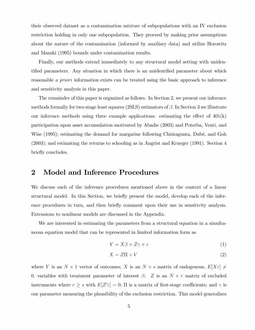
2 Model and Inference Procedures

We discuss each of the inference procedures mentioned above in the context of a linear

structural model. In this Section, we briefly present the model, develop each of the infer-

ence procedures in turn, and then briefly comment upon their use in sensitivity analysis.

Extensions to nonlinear models are discussed in the Appendix.

We are interested in estimating the parameters from a structural equation in a simulta-

neous equation model that can be represented in limited information form as

Y = Xβ + Zγ + ε (1)

X = ZΠ+ V (2)

where Y is an N × 1 vector of outcomes; X is an N × s matrix of endogenous, E[Xε] 6=

0, variables with treatment parameter of interest β; Z is an N × r matrix of excluded

instruments where r ≥ s with E[Z 0ε] = 0; Π is a matrix of first-stage coefficients; and γ is

our parameter measuring the plausibility of the exclusion restriction. This model generalizes

5

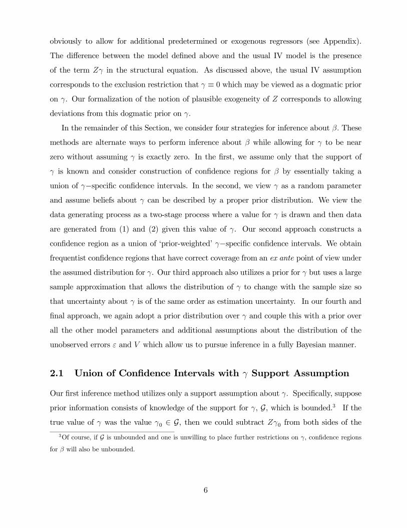
obviously to allow for additional predetermined or exogenous regressors (see Appendix).

The difference between the model defined above and the usual IV model is the presence

of the term Zγ in the structural equation. As discussed above, the usual IV assumption

corresponds to the exclusion restriction that γ ≡ 0 which may be viewed as a dogmatic prior

on γ. Our formalization of the notion of plausible exogeneity of Z corresponds to allowing

deviations from this dogmatic prior on γ.

In the remainder of this Section, we consider four strategies for inference about β. These

methods are alternate ways to perform inference about β while allowing for γ to be near

zero without assuming γ is exactly zero. In the first, we assume only that the support of

γ is known and consider construction of confidence regions for β by essentially taking a

union of γ−specific confidence intervals. In the second, we view γ as a random parameter

and assume beliefs about γ can be described by a proper prior distribution. We view the

data generating process as a two-stage process where a value for γ is drawn and then data

are generated from (1) and (2) given this value of γ. Our second approach constructs a

confidence region as a union of ‘prior-weighted’ γ−specific confidence intervals. We obtain

frequentist confidence regions that have correct coverage from an ex ante point of view under

the assumed distribution for γ. Our third approach also utilizes a prior for γ but uses a large

sample approximation that allows the distribution of γ to change with the sample size so

that uncertainty about γ is of the same order as estimation uncertainty. In our fourth and

final approach, we again adopt a prior distribution over γ and couple this with a prior over

all the other model parameters and additional assumptions about the distribution of the

unobserved errors ε and V which allow us to pursue inference in a fully Bayesian manner.

2.1 Union of Confidence Intervals with γ Support Assumption

Our first inference method utilizes only a support assumption about γ. Specifically, suppose

prior information consists of knowledge of the support for γ, G, which is bounded.3 If the

true value of γ was the value γ0 ∈ G, then we could subtract Zγ0 from both sides of the

3Of course, if G is unbounded and one is unwilling to place further restrictions on γ, confidence regions

for β will also be unbounded.

6

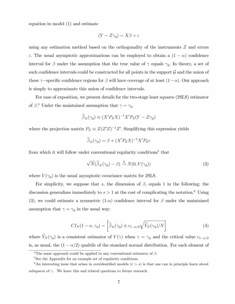
equation in model (1) and estimate

(Y − Zγ0) = Xβ + ε

using any estimation method based on the orthogonality of the instruments Z and errors

ε. The usual asymptotic approximations can be employed to obtain a (1 − α) confidence

interval for β under the assumption that the true value of γ equals γ0. In theory, a set of

such confidence intervals could be constructed for all points in the support G and the union of

these γ−specific confidence regions for β will have coverage of at least (1−α). Our approach

is simply to approximate this union of confidence intervals.

For ease of exposition, we present details for the two-stage least squares (2SLS) estimator

of β.4 Under the maintained assumption that γ = γ0

bβN(γ0) ≡ (X 0PZX)−1X 0PZ(Y − Zγ0)

where the projection matrix PZ ≡ Z(Z 0Z)−1Z 0. Simplifying this expression yields

bβN(γ0) = β + (X 0PZX)−1X 0PZε

from which it will follow under conventional regularity conditions5 that

√N(bβN(γ0)− β)

d→ N(0, V (γ0)) (3)

where V (γ0) is the usual asymptotic covariance matrix for 2SLS.

For simplicity, we suppose that s, the dimension of β, equals 1 in the following; the

discussion generalizes immediately to s > 1 at the cost of complicating the notation.6 Using

(3), we could estimate a symmetric (1-α) confidence interval for β under the maintained

assumption that γ = γ0 in the usual way:

CIN(1− α, γ0) =

∙bβN(γ0)± c1−α/2

qbVN(γ0)/N¸ (4)

where bVN(γ0) is a consistent estimator of V (γ) when γ = γ0 and the critical value c1−α/2

is, as usual, the (1− α/2) qualtile of the standard normal distribution. For each element of

4The same approach could be applied to any conventional estimator of β.5See the Appendix for an example set of regularity conditions.6An interesting issue that arises in overidentified models (r > s) is that one can in principle learn about

subspaces of γ. We leave this and related questions to future research.

7

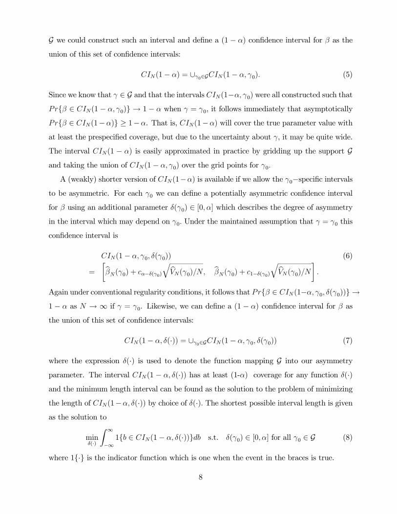
G we could construct such an interval and define a (1 − α) confidence interval for β as the

union of this set of confidence intervals:

CIN(1− α) = ∪γ0∈GCIN(1− α, γ0). (5)

Since we know that γ ∈ G and that the intervals CIN(1−α, γ0) were all constructed such that

Prβ ∈ CIN(1− α, γ0) → 1− α when γ = γ0, it follows immediately that asymptotically

Prβ ∈ CIN(1−α) ≥ 1−α. That is, CIN(1−α) will cover the true parameter value with

at least the prespecified coverage, but due to the uncertainty about γ, it may be quite wide.

The interval CIN(1 − α) is easily approximated in practice by gridding up the support G

and taking the union of CIN(1− α, γ0) over the grid points for γ0.

A (weakly) shorter version of CIN(1−α) is available if we allow the γ0−specific intervals

to be asymmetric. For each γ0 we can define a potentially asymmetric confidence interval

for β using an additional parameter δ(γ0) ∈ [0, α] which describes the degree of asymmetry

in the interval which may depend on γ0. Under the maintained assumption that γ = γ0 this

confidence interval is

CIN(1− α, γ0, δ(γ0)) (6)

=

∙bβN(γ0) + cα−δ(γ0)

qbVN(γ0)/N, bβN(γ0) + c1−δ(γ0)

qbVN(γ0)/N¸ .Again under conventional regularity conditions, it follows that Prβ ∈ CIN(1−α, γ0, δ(γ0))→

1 − α as N → ∞ if γ = γ0. Likewise, we can define a (1 − α) confidence interval for β as

the union of this set of confidence intervals:

CIN(1− α, δ(·)) = ∪γ0∈GCIN(1− α, γ0, δ(γ0)) (7)

where the expression δ(·) is used to denote the function mapping G into our asymmetry

parameter. The interval CIN(1 − α, δ(·)) has at least (1-α) coverage for any function δ(·)

and the minimum length interval can be found as the solution to the problem of minimizing

the length of CIN(1−α, δ(·)) by choice of δ(·). The shortest possible interval length is given

as the solution to

minδ(·)

Z ∞

−∞1b ∈ CIN(1− α, δ(·))db s.t. δ(γ0) ∈ [0, α] for all γ0 ∈ G (8)

where 1· is the indicator function which is one when the event in the braces is true.

8

In practice, we anticipate that often there will be only modest gains from calculating

the shortest interval via solving the minimization problem in (8) compared with the easy-

to-compute union of symmetric intervals (5). In situations where the variation in bβN(γ0)across γ0 values is large relative to the estimated standard errors, even if all of the weight at

the extreme values of bβN(γ0) is concentrated in one tail the changes to the overall intervallength will be small. In addition, when the standard errors are much larger than the range ofbβN(γ0) estimates there will also be little scope for moving away from equal tailed intervals.

The chief drawback of the union of confidence intervals approach is that the resulting

confidence regions may be large. In a sense, this approach produces valid intervals by

requiring correct coverage in every possible case, including the worst. Alternatively, one

may be willing to use more prior information than just the support of γ. In particular, if

one is willing to assign a prior distribution over potential values for γ, intervals that use this

additional information are feasible. These intervals will generally be much narrower than

those produced using the bounds given above and can be simple to construct in practice.

2.2 Unions of ‘Prior-weighted’ confidence intervals

In this approach, we view prior probabilities as equivalent to the first stage of the following

two-stage DGP. Nature first draws γ from a distribution F with support G that corresponds

to the researcher’s specified proper prior distribution of beliefs about γ. The data are

then generated via the model (1) and (2). Since the value of the draw for γ is unknown, we

construct confidence regions that will have correct ex ante coverage under repeated sampling

from this two-step DGP.

We begin by defining another γ0-specific confidence interval with an additional degree of

freedom, allowing the confidence level to also depend on γ0. Thus we define a (1 − a(γ0))

confidence interval for β conditional on γ = γ0 as

CIN(1− a(γ0), γ0, δ(γ0)) (9)

=

∙bβN(γ0) + ca(γ0)−δ(γ0)

qbVN(γ0)/N, bβN(γ0) + c1−δ(γ0)

qbVN(γ0)/N¸ .Without any information about the distribution of potential values of γ beyond a support

condition, the only way to insure correct ex ante coverage of (1-α) is to set a(·) ≡ α and

9

take the union of confidence sets as was done above. This union of confidence intervals is a

natural place to start in the present context and will certainly produce a confidence region

for β that has correct coverage. However, the additional information available in a specified

prior over possible values for γ opens the possibility of achieving correct coverage with a

shorter interval by ‘weighting’ the confidence intervals according to the prior.

We define a union of ‘prior-weighted’ confidence intervals as

CIF,N(1− α, a(·), δ(·)) = ∪γ0∈GCIN(1− a(γ0), γ0, δ(γ0)) (10)

subject to

δ(γ0) ∈ [0, α(γ0)] andZGα(γ0)dF (γ0) = α

where CIN(1 − a(γ0), γ0, δ(γ0)) is a (1 − a(γ0))(possibly asymmetric) confidence interval

given γ = γ0 defined by (9). The constraintRG α(γ0)dF (γ0) = α ensures ex ante coverage

of (1-α), under the prior distribution F. Under regularity conditions, CIF,N(1− α, a(·), δ(·))

has coverage at least (1− α), as N →∞ (See Appendix).

The ability to choose the level of the confidence intervals (1 − a(γ0)) to vary according

to hypothesized value of γ0 allows us to implicitly ‘weight’ the confidence intervals obtained

for different values of γ0 according to prior beliefs about the likelihood of particular values

of γ. We are able to choose low levels of confidence for unlikely values of γ and higher levels

of confidence for more likely values. Under the specified distribution for γ, the union of

these regions will have correct coverage and, because an additional choice variable has been

added, will be (weakly) shorter than the bounds in Section 2.1 if the functions a(·) and δ(·)

are chosen well. The choices of a(·) and δ(·) that minimize the size of the interval solve the

following problem:

mina(·),δ(·)

Z ∞

−∞1b ∈ CIF,N(1− α, a(·), δ(·))db. (11)

Note that this problem corresponds to a modification of the choice problem in Section 2.1

for the minimum-length interval given only support information. The modification is to

introduce an additional free parameter a(·), so the interval corresponding to the solution of

(11) will always be weakly smaller than the confidence region obtained without using the

distributional information about γ.

To illustrate the difference between the approach in Section 2.1 and our union of ‘prior-

10

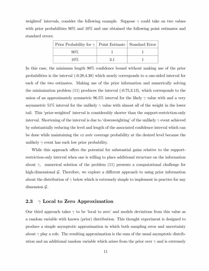
weighted’ intervals, consider the following example. Suppose γ could take on two values

with prior probabilities 90% and 10% and one obtained the following point estimates and

standard errors:

Prior Probability for γ Point Estimate Standard Error

90% 1 1

10% 3.1 1

In this case, the minimum length 90% confidence bound without making use of the prior

probabilities is the interval (-0.28,4.38) which nearly corresponds to a one-sided interval for

each of the two estimates. Making use of the prior information and numerically solving

the minimization problem (11) produces the interval (-0.75,3.13), which corresponds to the

union of an approximately symmetric 96.5% interval for the likely γ value with and a very

asymmetric 51% interval for the unlikely γ value with almost all of the weight in the lower

tail. This ‘prior-weighted’ interval is considerably shorter than the support-restriction-only

interval. Shortening of the interval is due to ‘downweighting’ of the unlikely γ event achieved

by substantially reducing the level and length of the associated confidence interval which can

be done while maintaining the ex ante coverage probability at the desired level because the

unlikely γ event has such low prior probability.

While this approach offers the potential for substantial gains relative to the support-

restriction-only interval when one is willing to place additional structure on the information

about γ, numerical solution of the problem (11) presents a computational challenge for

high-dimensional G. Therefore, we explore a different approach to using prior information

about the distribution of γ below which is extremely simple to implement in practice for any

dimension G.

2.3 γ Local to Zero Approximation

Our third approach takes γ to be ‘local to zero’ and models deviations from this value as

a random variable with known (prior) distribution. This thought experiment is designed to

produce a simple asymptotic approximation in which both sampling error and uncertainty

about γ play a role. The resulting approximation is the sum of the usual asymptotic distrib-

ution and an additional random variable which arises from the prior over γ and is extremely

11

simple to work with. One ends up with the usual approximation plus a term which increases

dispersion depending on the strength of prior beliefs about the plausibility of the exclusion

restriction.

In this approach to plausible exogeneity, we model γ as being local to zero.7 Explicitly

referencing the dependence of γ upon the sample size via a subscript N we represent γ in

structural equation (1) as

γN = η/√N where η ∼ G. (12)

We assume η is independent of X, Z, and ε. In our approach we equate prior information

about plausible values of γ with knowledge of the distribution G.

The normalization by√N in the definition of γN is designed to produce asymptotics

in which the uncertainty about exogeneity and usual sampling error are of the same order

and so both factor into the asymptotic distribution. If instead, γN were equal to η/N b

for b < 1/2, the asymptotic behavior would be determined completely by the ‘exogeneity

error’ η/N b; and if b were greater than 1/2, the limiting distribution would be determined

completely by the usual sampling behavior. The modeling device we use may be regarded

as a thought experiment designed to produce an approximation in which both ‘exogeneity

error’ and sampling error play a role and not as the actual DGP. To the extent that both

sources of error do play a role, the approximation will tend to be more accurate than the

approximation obtained when either source of error dominates.

7It is a straightforward extension to model γ as being local to any known value.

12

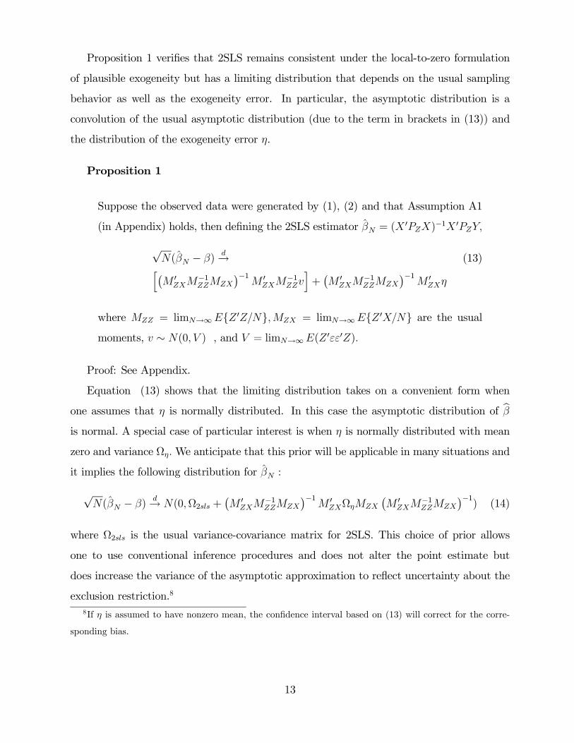
Proposition 1 verifies that 2SLS remains consistent under the local-to-zero formulation

of plausible exogeneity but has a limiting distribution that depends on the usual sampling

behavior as well as the exogeneity error. In particular, the asymptotic distribution is a

convolution of the usual asymptotic distribution (due to the term in brackets in (13)) and

the distribution of the exogeneity error η.

Proposition 1

Suppose the observed data were generated by (1), (2) and that Assumption A1

(in Appendix) holds, then defining the 2SLS estimator βN = (X0PZX)

−1X 0PZY,

√N(βN − β)

d→ (13)h¡M 0

ZXM−1ZZMZX

¢−1M 0

ZXM−1ZZv

i+¡M 0

ZXM−1ZZMZX

¢−1M 0

ZXη

where MZZ = limN→∞EZ 0Z/N,MZX = limN→∞EZ 0X/N are the usual

moments, v ∼ N(0, V ) , and V = limN→∞E(Z 0εε0Z).

Proof: See Appendix.

Equation (13) shows that the limiting distribution takes on a convenient form when

one assumes that η is normally distributed. In this case the asymptotic distribution of bβis normal. A special case of particular interest is when η is normally distributed with mean

zero and variance Ωη.We anticipate that this prior will be applicable in many situations and

it implies the following distribution for βN :

√N(βN − β)

d→ N(0,Ω2sls +¡M 0

ZXM−1ZZMZX

¢−1M 0

ZXΩηMZX

¡M 0

ZXM−1ZZMZX

¢−1) (14)

where Ω2sls is the usual variance-covariance matrix for 2SLS. This choice of prior allows

one to use conventional inference procedures and does not alter the point estimate but

does increase the variance of the asymptotic approximation to reflect uncertainty about the

exclusion restriction.8

8If η is assumed to have nonzero mean, the confidence interval based on (13) will correct for the corre-

sponding bias.

13

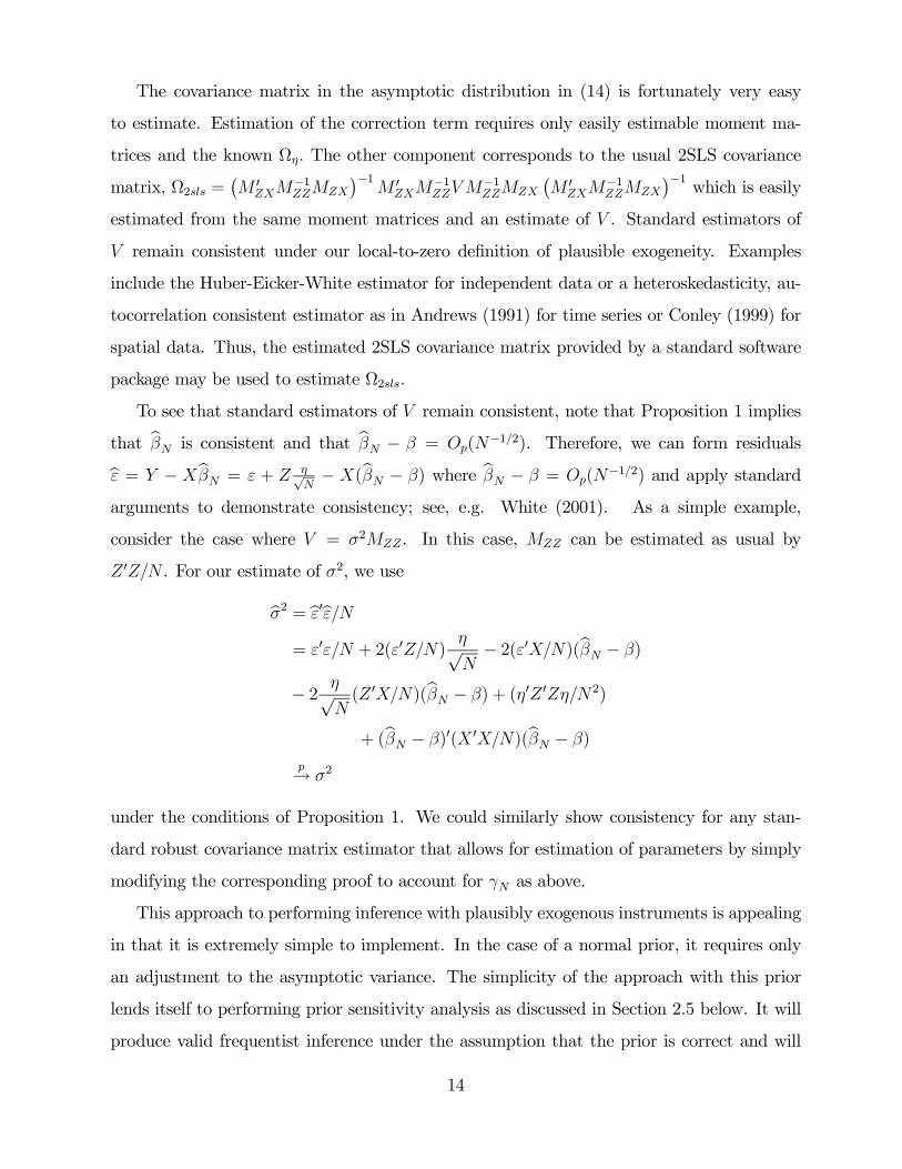
The covariance matrix in the asymptotic distribution in (14) is fortunately very easy

to estimate. Estimation of the correction term requires only easily estimable moment ma-

trices and the known Ωη. The other component corresponds to the usual 2SLS covariance

matrix, Ω2sls =¡M 0

ZXM−1ZZMZX

¢−1M 0

ZXM−1ZZVM

−1ZZMZX

¡M 0

ZXM−1ZZMZX

¢−1which is easily

estimated from the same moment matrices and an estimate of V . Standard estimators of

V remain consistent under our local-to-zero definition of plausible exogeneity. Examples

include the Huber-Eicker-White estimator for independent data or a heteroskedasticity, au-

tocorrelation consistent estimator as in Andrews (1991) for time series or Conley (1999) for

spatial data. Thus, the estimated 2SLS covariance matrix provided by a standard software

package may be used to estimate Ω2sls.

To see that standard estimators of V remain consistent, note that Proposition 1 implies

that bβN is consistent and that bβN − β = Op(N−1/2). Therefore, we can form residualsbε = Y − XbβN = ε + Z η√

N− X(bβN − β) where bβN − β = Op(N

−1/2) and apply standard

arguments to demonstrate consistency; see, e.g. White (2001). As a simple example,

consider the case where V = σ2MZZ. In this case, MZZ can be estimated as usual by

Z 0Z/N . For our estimate of σ2, we use

bσ2 = bε0bε/N= ε0ε/N + 2(ε0Z/N)

η√N− 2(ε0X/N)(bβN − β)

− 2 η√N(Z 0X/N)(bβN − β) + (η0Z 0Zη/N2)

+ (bβN − β)0(X 0X/N)(bβN − β)

p→ σ2

under the conditions of Proposition 1. We could similarly show consistency for any stan-

dard robust covariance matrix estimator that allows for estimation of parameters by simply

modifying the corresponding proof to account for γN as above.

This approach to performing inference with plausibly exogenous instruments is appealing

in that it is extremely simple to implement. In the case of a normal prior, it requires only

an adjustment to the asymptotic variance. The simplicity of the approach with this prior

lends itself to performing prior sensitivity analysis as discussed in Section 2.5 below. It will

produce valid frequentist inference under the assumption that the prior is correct and will

14

provide robustness relative to the conventional approach (that assumes γ ≡ 0) even when

incorrect.

2.4 Full Bayesian Analysis

In the previous subsections, we have considered two types of prior information: knowledge

of the support of γ and explicit prior distributions over γ. A Bayesian approach to inference

is a natural complement to these methods that incorporate prior information about part of

the model defined by (1) and (2). Of course, Bayesian inference will require priors over the

other model parameters as well as assumptions regarding the distribution of the error terms

to complete the model likelihood. We let p(Data|β, γ,Π, θ) be the likelihood of the data

conditional on the treatment and reduced form parameters, (β, γ,Π), and the parameters

characterizing the distribution of the error terms, θ. Our inference will be based on the

posterior distribution for β, Π, and θ given the data, integrating out γ :

p(β,Π, θ|Data) ∝Z

p(Data|β, γ,Π, θ)pγ(γ|β,Π, θ)pβ,Π,θ(β,Π, θ)dγ (15)

where pβ,Π,θ(β,Π, θ) is the prior distribution over the model parameters and pγ(γ|β,Π, θ)

is the prior distribution over γ which, in principle, is allowed to depend on all other model

parameters. We note that allowing this dependence is straightforward in the Bayesian setting

and allows one a great deal of flexibility in the way prior information regarding the ‘exogeneity

error’ γ is incorporated. For example, it is simple to allow prior beliefs that γ is likely to

be a small proportion of the value of β or beliefs about the exclusion restriction in terms

of the unidentified population R2 of the regression of Z on the structural error in which

case the prior would depend on the distributional parameters θ. Either of these approaches

to prior information is cumbersome in the frequentist frameworks outlined in the previous

Subsections 2.1 to 2.3.

An arbitrarily tight prior centered on zero for γ is equivalent with the IV exclusion

restriction. The extent to which inference about β, i.e. its posterior distribution, depends on

the exclusion restriction can be determined by prior sensitivity analysis. As we increase the

spread of the prior on γ, we weaken the restriction by allowing for the instruments to have

some ‘direct’ effect on y. In a typical analysis, we will consider a series of prior settings and

15

investigate the effect of loosening the prior on γ upon inference for the structural parameter,

β.

In the Bayesian analyses reported in our empirical examples, we consider possible priors

for γ that do and do not depend upon β :

Prior 1: γ ∼ N(μ, δ2I) (16)

Prior 2: γ|β ∼ N(0, δ2β2I). (17)

With prior 1, we will need to have some idea of the size of the direct effect γ without

reference to the treatment effect β. This information may come from other data sources, or

we may have some intuition about potential benchmark values for γ. We anticipate using

Prior 2 with δ small, based on the idea that the effects of Z on Y should be smaller than

the effect of X on Y and that the treatment effect could be used to benchmark γ were it

available. This prior is one representation of the core idea that the exclusion restriction need

not hold exactly but that deviations should be small. Prior 2 is a non-standard prior in the

Bayesian simultaneous equations literature where independent priors are typically used for

model coefficients. Prior 2 assesses the conditional prior distribution of γ given β and can

be coupled with a standard diffuse normal prior on β.

Given the likelihood and the priors, the chief difficulty in conducting Bayesian inference is

in evaluating the posterior distribution which will typically be done using MCMC methods.

There are a number of approaches that may be used to sample from the posterior distribution

(15). For ease of exposition, we use a Gaussian distribution for (ε, V ). With this error

distribution and linearity of (1) and (2), it is convenient to use conditionally conjugate

Gaussian priors for parameters. We couple these with an inverse Wishart prior over the

variance covariance matrix of the errors, (ε, V ), also conditionally conjugate, to form the

basis of a Gibbs sampler. Rossi et al (2005) provide an efficient Gibbs sampler for this case

which we employ in obtaining the estimation results in Section 3 below.9 The only difference

between our sampler and the sampler of Rossi et al (2005) is the inclusion of the term

involving γ in the structural equation. We briefly illustrate how this changes the sampler in

the Appendix.9The data were scaled by the standard deviation of Y and then the priors used were Σ ≡ Cov(ε, V ) ∼

Inverse Wishart(5, 5I), and β ∼ N(0, 100).

16

We could of course employ Bayesian methods for any parametric likelihood and a non-

parametric approach via flexibly approximating an arbitrary likelihood is also feasible. For

example, Conley et al (2006) demonstrate how a fully non-parametric Bayesian inference

can be conducted by using a Dirichlet Process prior for the distribution of the error terms.

This procedure can be viewed as using a mixture of normals distribution for the error terms

where the number of mixture components is random and potentially infinite. The MCMC

methods used to implement this model and prior are completely modular in the sense that,

for any given draw, the distribution of the error terms is a mixture of normals with a known

classification of each observation to a given normal mixture component. This means that

any priors specified for a one component model (i.e. a model with normally distributed error

terms) can be extended trivially (with no modification of code) to the Dirichlet Process prior;

that is, the approach outlined above will carry over to this more general model for (ε, V ).

It is important to note that full Bayesian analysis facilitates exact small sample inference

as well as considerable flexibility in prior specification and sensitivity analysis. There are

certainly many applications where small sample considerations are paramount, e.g. due to

weak or large numbers of instruments. If relatively diffuse priors are used on β and π and

a sufficiently flexible distribution is specified for (ε, V ), the requirements of a full Bayesian

analysis are only modestly higher than the methods above using large sample approximations.

All approaches hinge on a careful assessment of the prior on γ as well as sensitivity analysis.

2.5 Sensitivity Analysis

In the preceding subsections, we outlined four basic approaches to inference that may be

adopted in situations in which there is uncertainty about an IV exclusion restriction. In

each, we model the specification error through an unidentified parameter γ and proceed to

do inference utilizing assumptions about possible values for this parameter. We anticipate

that the main benefit of our procedures will come from applying them under more than

one assumption regarding γ and comparing results for β estimates across assumptions, con-

ducting sensitivity analysis. This sort of sensitivity analysis gives the researcher substantial

insight into how confident one needs to be about the exclusion restriction for the results of

chief interest to remain largely unchanged.

17

The exact approach to conducting the sensitivity analysis will vary slightly under each

of the different methods/operational definitions of plausible exogeneity. For example, in the

support-restriction-only approach in Section 2.1 with one instrument, one could take G to be

an interval [−δ, δ] and plot a confidence interval of interest versus many different values of δ.

One could then assess how large the support of possible values of γ would need to be before

the confidence intervals became uninformative about a hypothesis of interest. For the other

approaches presented in Sections 2.2 through 2.4 a fully specified prior distribution over G

is required, and thus sensitivity analysis may proceed by choosing different distributions for

γ. This approach to sensitivity analysis can be readily done by selecting a parametric family

for γ and then varying the distributional parameters. For example, with one instrument,

one could take γ (or η in the local definition in Section 2.3) to be normally distributed with

variance σ2. Again one could compute confidence intervals (or credibility intervals in the

case of Bayesian inference) as a function of σ2 and assess how much uncertainty about the

exclusion restriction, as measured by the prior variance σ2, would result in the confidence

intervals becoming uninformative about a null hypothesis of interest.

We note that this approach to sensitivity analysis is most easily implemented using the

local-to-zero model of plausible exogeneity in Section 2.3 under the prior assumption that

η ∼ N(0,Ωη). In this case, the prior over the specification error influences only the dispersion

of the asymptotic distribution given in (14) and this influence has a simple analytic form.

Given estimates of this asymptotic variance for various Ωη, confidence intervals (or other

statistics of interest) may easily be obtained and one can quickly assess the magnitudes of

exogeneity error that would result in substantial deviations from conventional inference using

an exact exclusion restriction.

3 Empirical Examples:

This Section presents three illustrative example applications of our methods: the effect of

participating in a 401(k) plan upon accumulated assets, the demand for margarine, and

the returns to schooling. We have chosen these three to illustrate both the breadth of po-

tential applications for our methods as well as some of the variety of specifications for γ

18

priors that may prove useful. The 401(k) application provides an example where some re-

searchers may anticipate a violation of the exclusion restriction. Our methods can readily

accommodate this by using priors for γ that are not centered at zero. In demand estima-

tion priors for a wholesale price direct effect, γ, might be usefully specified as depending on

the price elasticity of interest. This is easily captured by using priors for γ that depend

on β. Finally, the returns-to-schooling application provides an example scenario where a

prior for γ can be grounded in existing research. In all applications we assume indepen-

dence across observations and estimate covariance matrices using the Huber-Eicker-White

heteroskedasticity-consistent covariance matrix estimator.

3.1 Effect of 401(k) Participation upon Asset Accumulation

Our first example application examines the effect of 401(k) plan participation upon asset

accumulation. Our data are those of Poterba, Venti, and Wise (1995), Abadie (2003),

Benjamin (2003), and Chernozhukov and Hansen (2004) from wave 4 of the 1990 Survey

of Income and Program Participation which consists of observations on 9915 households

with heads aged 25-64 with at least one adult employed (excluding self-employed). The

outcome of interest is net financial assets (1991 dollars) and the treatment of interest is an

indicator for 401(k) participation in the following regression:

Net Financial Assets = β × 401(k) participation+Xλ+ Zγ + u.

X is a is a vector of covariates that includes five age category indicators, seven income

category indicators, family size, four education category indicators, a marital status indica-

tor, a two-earner status indicator, a defined benefit pension indicator, an IRA participation

indicator, and a home ownership indicator. The instrument Z is an indicator for 401(k)

plan eligibility: whether an individual in the household works for a firm with a 401(k) plan.

Further details and descriptive statistics can be found in, for example, Benjamin (2003) or

Chernozhukov and Hansen (2004).

An argument for 401(k) eligibility being a valid instrument is put forth in a series of

articles by Poterba, Venti, and Wise (1994, 1995, 1996). These authors argue that eligibility

for a 401(k) can be taken as exogenous given income and 401(k) eligibility and participation

19

are of course correlated. Their main claim is the fact that eligibility is determined by

employers and so is plausibly taken as exogenous conditional on covariates. In particular, if

individuals made employment decisions based on income and within jobs classified by income

categories it is random whether or not a firm offers a 401(k) plan, the exclusion restriction

would be justified. Poterba, Venti, and Wise (1996) contains an overview of suggestive

evidence based on pre-program savings used to substantiate this claim. Of course, the

argument for the exogeneity of 401(k) eligibility is hardly watertight. For example, one

might conjecture that firms which introduced 401(k)’s did so due to pressure from their

employees implying that firms with plans are those with employees who really like saving.

People might also select employment on the basis of available retirement packages in addition

to income. For these and other reasons, Engen, Gale, and Sholz (1996) argue that 401(k)

eligibility is not a valid instrument and is positively related to the unobservables affecting

financial asset accumulation.

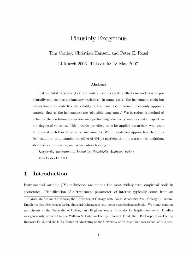
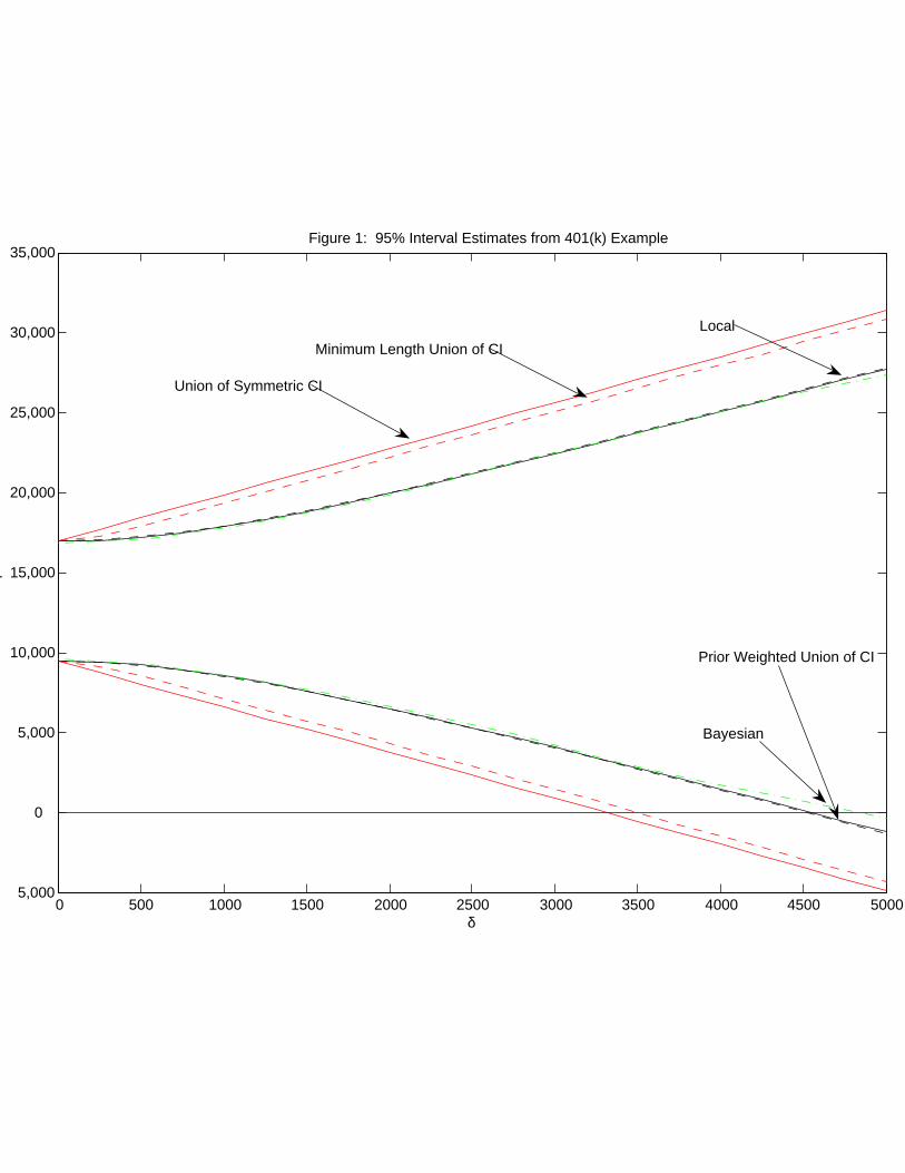
Figure 1 displays results for the full array of our methods with γ priors centered at

zero. This figure plots five sets of confidence intervals for an array of assumptions about

prior information indexed by the parameter δ. The widest set of solid lines presents 95%

confidence intervals using the method in Section 2.1 with a union of symmetric γ0-specific

intervals. Their corresponding support restrictions are of the form γ ∈ [−2δ,+2δ]. The

dashed lines that lie just inside of them are the minimum-length bound from Section 2.1

with the same [−2δ,+2δ] support condition. The remaining three intervals are very close to

each other, well within the support-restriction-only intervals. Among this set of lines: the

dashed lines correspond to the union of prior-weighted intervals approach from Section 2.2

with γ prior of N(0, δ2), the solid lines correspond to the local-to-zero method of Section 2.3

with γ prior of N(0, δ2), and the dot-dash lines are 95% Bayesian credibility intervals, .025

and .975 quantiles of the posterior for β, from Section 2.4 again obtained with a γ prior of

N(0, δ2).

The dominant feature of Figure 1 is that there are basically two sets of intervals, those

with support conditions only and those with a prior distribution for γ. It is important to

note that since the intervals constructed with support conditions necessarily require bounded

support, they are not strictly comparable with the Gaussian prior distributions. However,

20

we are confident that differences in support are not the cause of this discrepancy, it is due

to the introduction of the distributional information. Similar qualitative results to those

with Gaussian priors obtain using uniform priors with support [−2δ,+2δ]. The coincidence

of the other three intervals is a combination of their common priors and the large amount

of information in the data. The two support-restriction-only intervals are close in all our

example applications so will henceforth plot one of them to minimize clutter. Likewise, we

will omit plotting intervals for the prior-weighted union of confidence intervals as it is always

very close to the local-to-zero intervals (when they have common priors).

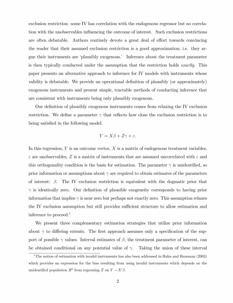
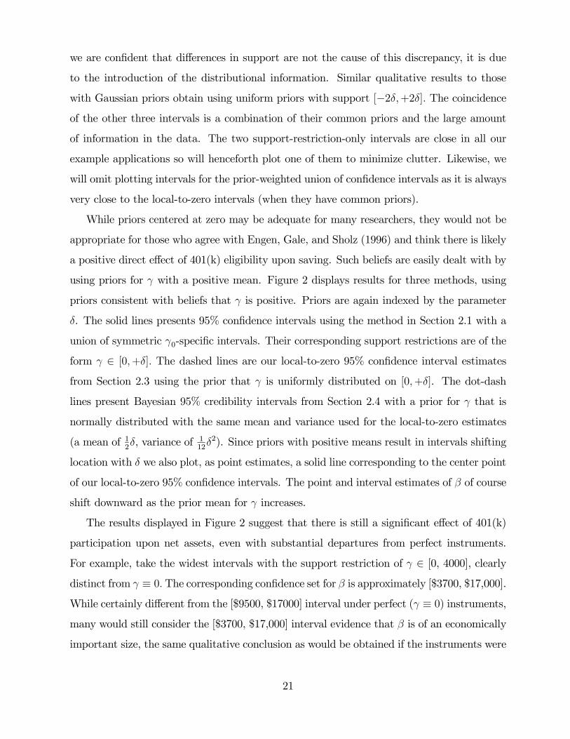
While priors centered at zero may be adequate for many researchers, they would not be

appropriate for those who agree with Engen, Gale, and Sholz (1996) and think there is likely

a positive direct effect of 401(k) eligibility upon saving. Such beliefs are easily dealt with by

using priors for γ with a positive mean. Figure 2 displays results for three methods, using

priors consistent with beliefs that γ is positive. Priors are again indexed by the parameter

δ. The solid lines presents 95% confidence intervals using the method in Section 2.1 with a

union of symmetric γ0-specific intervals. Their corresponding support restrictions are of the

form γ ∈ [0,+δ]. The dashed lines are our local-to-zero 95% confidence interval estimates

from Section 2.3 using the prior that γ is uniformly distributed on [0,+δ]. The dot-dash

lines present Bayesian 95% credibility intervals from Section 2.4 with a prior for γ that is

normally distributed with the same mean and variance used for the local-to-zero estimates

(a mean of 12δ, variance of 1

12δ2). Since priors with positive means result in intervals shifting

location with δ we also plot, as point estimates, a solid line corresponding to the center point

of our local-to-zero 95% confidence intervals. The point and interval estimates of β of course

shift downward as the prior mean for γ increases.

The results displayed in Figure 2 suggest that there is still a significant effect of 401(k)

participation upon net assets, even with substantial departures from perfect instruments.

For example, take the widest intervals with the support restriction of γ ∈ [0, 4000], clearly

distinct from γ ≡ 0. The corresponding confidence set for β is approximately [$3700, $17,000].

While certainly different from the [$9500, $17000] interval under perfect (γ ≡ 0) instruments,

many would still consider the [$3700, $17,000] interval evidence that β is of an economically

important size, the same qualitative conclusion as would be obtained if the instruments were

21

assumed perfect.

3.2 Demand for Margarine

Our second example application concerns price endogeneity in demand estimation, a canon-

ical econometric problem. We use as our example the problem of estimating demand for

margarine using the data of Chintagunta, Dubé, and Goh (2003) . The sample consists of

weekly purchases and prices for the 4 most popular brands of margarine in the Denver area

for 117 weeks from January 1993 to March 1995. Pooling across brands, we estimate the

following model:

logShare = β log(retail price) +Xλ+ Zγ + u

where X includes brand indicators, feature and display indicators, and their interactions

with brand indicators. Following Chintagunta, Dube, and Goh (2003) we use log wholesale

prices as an instrument, Z, for retail prices.

The argument for plausible exogeneity of wholesale prices is that they should primarily

vary in response to cost shocks and should be much less sensitive to retail demand shocks

than retail prices. In this example application, we illustrate the use of priors for γ that

depend on β. It seems quite possible that researchers would be comfortable assuming that

direct effect of a wholesale price could be benchmarked relative to the elasticity with respect

to the corresponding retail price.

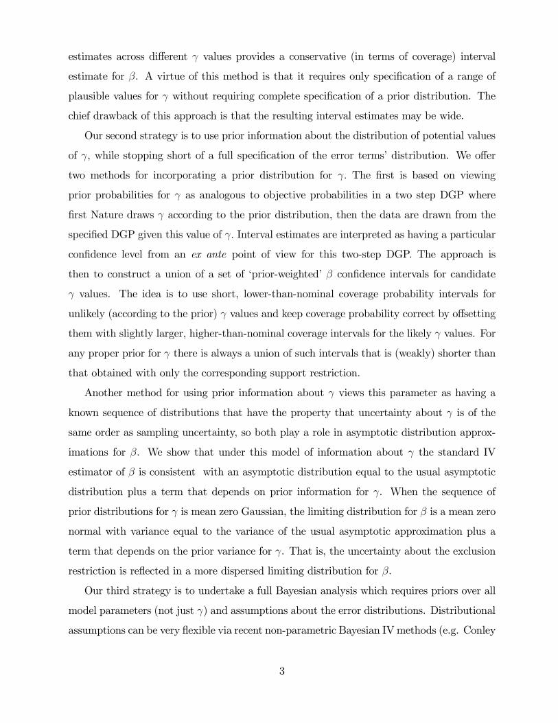
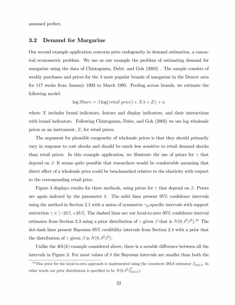
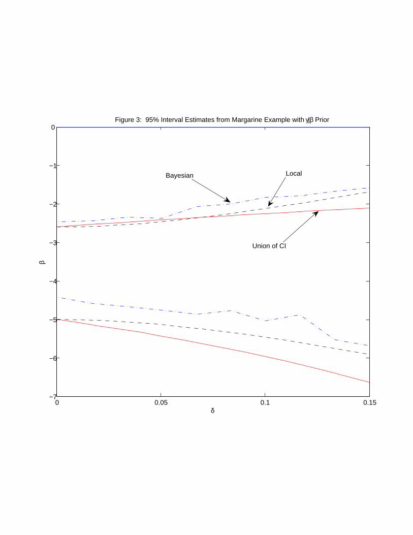
Figure 3 displays results for three methods, using priors for γ that depend on β. Priors

are again indexed by the parameter δ. The solid lines present 95% confidence intervals

using the method in Section 2.1 with a union of symmetric γ0-specific intervals with support

restriction γ ∈ [−2δβ,+2δβ]. The dashed lines are our local-to-zero 95% confidence interval

estimates from Section 2.3 using a prior distribution of γ given β that is N(0, δ2β2).10 The

dot-dash lines present Bayesian 95% credibility intervals from Section 2.4 with a prior that

the distribution of γ given β is N(0, δ2β2).

Unlike the 401(k) example considered above, there is a notable difference between all the

intervals in Figure 3. For most values of δ the Bayesian intervals are smaller than both the

10This prior for the local-to-zero approach is implemented using the consistent 2SLS estimator β2SLS . In

other words our prior distribution is specified to be N(0, δ2β2

2SLS).

22

others. The two factors of support differences and information in a full prior distribution

of course drive some of the discrepancy between the Bayesian and support-restiction-only

intervals. An additional source of discrepancy that is likely more important here than the

previous example application is the relatively small amount of information in the data. This

leads us to believe that much of the discrepancy between the Bayesian intervals and those

of the local-to-zero approximation is due to such ‘small sample effects.’ We anticipate that

many researchers may prefer the Bayesian intervals when faced with small to moderate

samples as a fully Bayesian approach provides exact small sample inference.

A qualitative conclusion from Figure 3 that is common across methods is that there

can be a substantial violation of the exclusion restriction without a major change in the

demand elasticity estimates. Inferences change little for a range of direct wholesale price

effects up to ten per cent of the size of the retail price effect. Take for example the local-

to-zero estimates, at δ = 0 the 95% confidence interval is (-5,-2.5) and at δ = 10% the 95%

confidence interval is (-5.5,-2.3). Put on a standard mark-up basis using the inverse elasticity

rule, the corresponding mark-up intervals are [20% to 40%] and [18% to 44%]. For many if

not all purposes, this is a small change in the implied mark-ups.

3.3 Returns to Schooling Using Quarter of Birth Instruments

Our final example application is estimating the returns to schooling using quarter of birth

as instruments as in Angrist and Krueger (1991). The sample consists of 329,509 males

from the 1980 U.S. Census who were born between 1930 and 1939. For this illustration, we

estimate the following model determining log wages:

logWage = βSchool +Xλ+ Zγ + u,

where the dependent variable is the log of the weekly wage, School is reported years of

schooling, andX is a vector of covariates consisting of state and year of birth fixed effects. To

sidestep weak and many instrument issues, we use only the three quarter of birth indicators,

with being born in the first quarter of the year as the excluded category, as instruments Z

and do not report results using interactions between quarter of birth and other regressors.11

11The first stage F-statistic from the specification with three instruments is 36.07 which is well within the

range where one might expect the usual asymptotic approximation to perform adequately.

23

The use of quarter of birth as an instrument is motivated by the fact that quarter of

birth is correlated with years of schooling due to compulsory schooling laws. The typical

law requires students to attend first grade in the year in which they turn age 6 and continue

school until age 16. This means that individuals born early in the year will usually be in the

middle of 10th grade when they turn 16 and can drop out while those born late in the year

will have finished 10th grade before they reach age 16.

Angrist and Krueger (1991) argue that quarter of birth is a valid instrument, correlated

with schooling attainment and uncorrelated with unobserved taste or ability factors which

influence earnings. Angrist and Krueger (1991) examine data from three decennial censuses

and find that people born in the first quarter of the year do indeed have less schooling on

average than those born later in the year. This correlation of quarter-of-birth and schooling

is uncontroversial. However, there is considerable debate about these instruments’ validity

due to correlation between birth quarter and other determinants of wages (e.g. Bound and

Jaeger (1996) and Bound, Jaeger, and Baker (1995) who argue that quarter of birth should

not be treated as exogenous). Bound, Jaeger, and Baker (1995) go beyond this in providing

well motivated ‘back of the envelope’ calculations of a plausible range for direct effects of

quarter of birth upon wages. They come up with an approximate magnitude of a direct

effect of quarter of birth upon wages of about 1%. Such calculations are directly useful in

our framework, informing our choice of prior for γ.

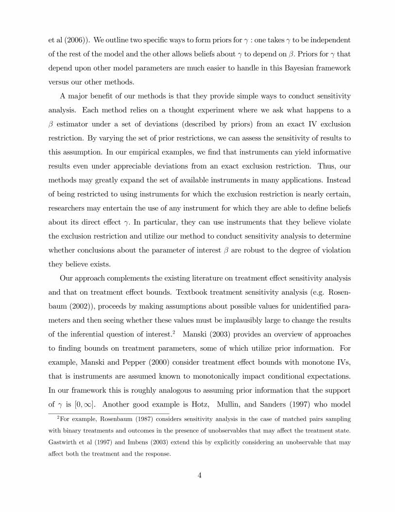
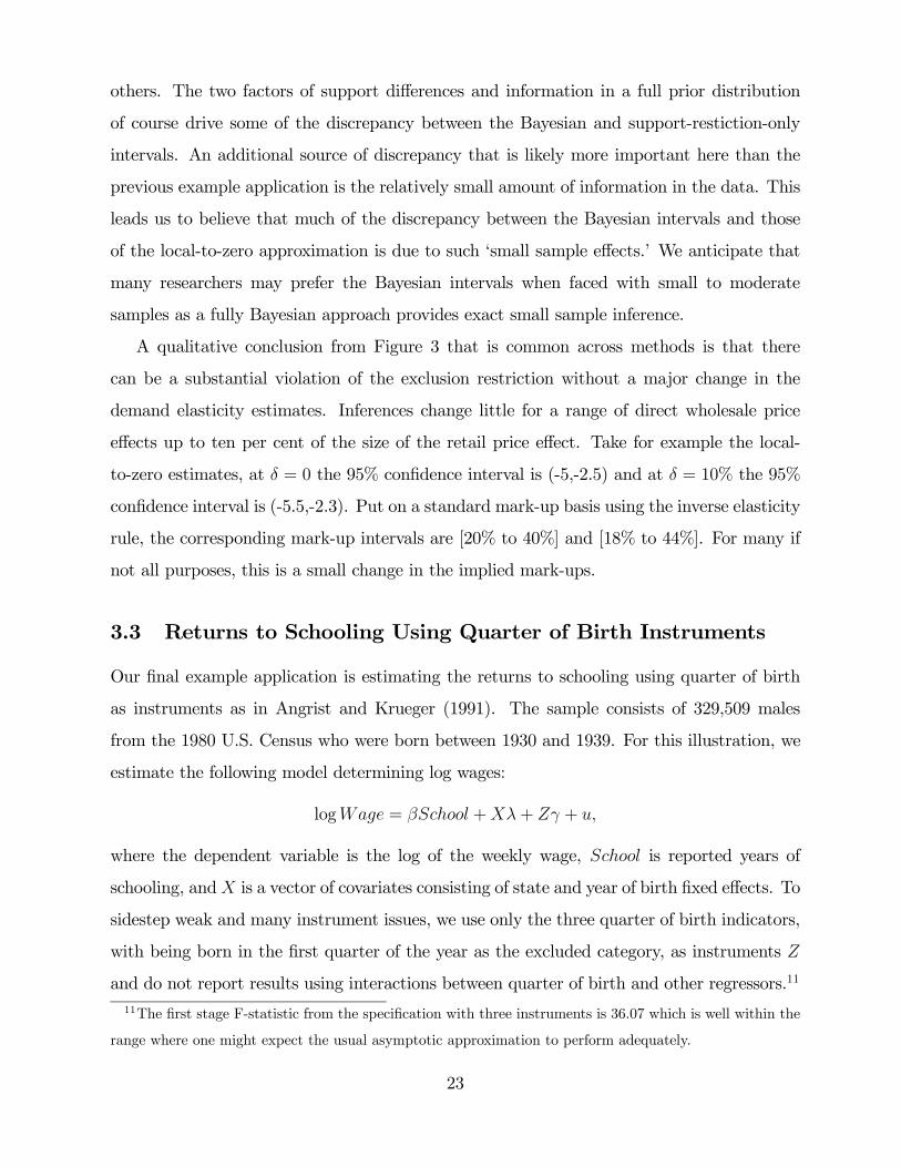
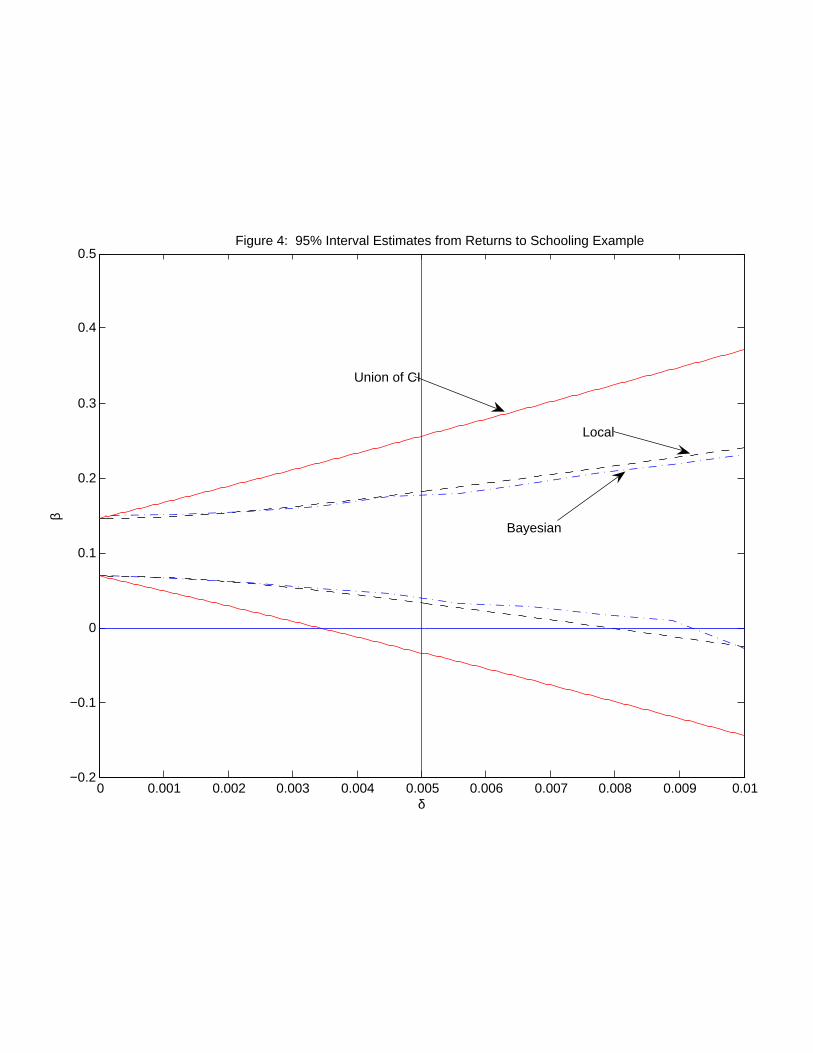
Results are displayed in Figure 4. This figure plots three sets of confidence intervals for

an array of assumptions about prior information indexed by the parameter δ. The solid

lines represent 95% confidence intervals using the method in Section 2.1 with a union of

symmetric γ0-specific intervals. Their corresponding support restrictions are of the form

γ ∈ [−2δ,+2δ]3. The dashed lines present 95% confidence intervals for our local-to-zero

method in Section 2.3 using priors for γ that are N(0, δ2I). Finally, the dot-dash lines

present Bayesian 95% credibility intervals using the model in Section 2.4 with N(0, δ2I)

priors for γ. The vertical line at δ = .005 provides a reference point for priors motivated

by the Bound, Jaeger, and Baker approximate magnitude for the direct effect of quarter of

birth of 1%.

The intervals in Figure 4 suggest that the data are essentially uninformative about the

24

returns to schooling under modest amounts of uncertainty regarding the exclusion restriction.

Using the Bound, Jaeger, and Baker (1995) calculations as an upper bound on the magnitude

of γ would require us to focus attention in a δ range near .005. At δ = .005, the local-to-zero

95% confidence interval for β is [ 3.4% to 18.3%], which we consider uninformative about the

returns to years of school. In order for these confidence intervals to be informative in our

judgment, prior beliefs regarding γ must be much more concentrated near zero. For example,

using the support-restriction-only intervals, one would need to be sure the magnitude of γ

was less than .002 to obtain a confidence interval for β that excluded 5%.

4 Conclusion

When using IV methods, researchers routinely provide informal arguments that their in-

struments satisfy the instrument exclusion restriction but recognize that this may only be

approximately true. Inference in these settings then typically proceeds under the assumption

that the IV exclusion restriction holds exactly and without formal sensitivity analysis of this

assumption. We have presented alternative approaches to inference that do not impose the

assumption that instruments exactly satisfy an exclusion restriction, they need only be plau-

sibly exogenous. Our methods provide an improved match between researchers’ assumptions

of plausible exogeneity and their methods of inference.

All of our approaches involve using some sort of prior information regarding the extent

of deviations from the exact exclusion restriction. Many of the usual arguments that re-

searchers use to justify exclusion restrictions are naturally viewed as providing information

about prior beliefs about violation of these restrictions. Our contribution is to provide a

practical method of incorporating this information. We provide a toolset for the applied

researcher to conduct sensitivity analysis with respect to the validity of a set of instruments.

We demonstrate the utility of our approach through three empirical applications. In two of

the three applications, a priori moderate violations of the exclusion restriction do not funda-

mentally alter qualitative conclusions regarding the parameters of interest. Useful inference

is clearly feasible with instruments that are only plausibly exogenous.

25

5 References

Abadie, A (2003): “Semiparametric Instrumental Variable Estimation of Treatment

Response Models,” Journal of Econometrics, 113(2), 231-263, 2003.

Andrews, D. W. K.. (1991): "Heteroskedasticity and Autocorrelation Consistent Covari-

ance Matrix Estimation," Econometrica, 59(3), 817-858.

Angrist, J. D., and A. Krueger (1991): "Does Compulsory Schooling Attendance Affect

Schooling and Earnings," Quarterly Journal of Economics, 106, 979-1014.

Benjamin, Daniel J. (2003). “Do 401(k)s Increase Saving? Evidence From Propensity

Score Subclassification,” Journal of Public Economics, 87(5-6), 1259-1290.

Bound, J., and D. A. Jaeger (1996): "On the validity of season of birth as an instrument

in wage equations: A comment on Angrist and Krueger’s ’Does compulsory attendance affect

schooling and earnings?’," NBER Working Paper 5835.

Bound, J., D. A. Jaeger, and R. M. Baker (1995): "Problems with Instrumental Variables

EstimationWhen the Correlation Between the Instruments and the Endogenous Explanatory

Variable is Weak," Journal of the American Statistical Association, 90(430), 443-450.

Chernozhukov V. and C. Hansen (2004): “The Impact of 401K Participation on Savings:

an IV-QR Analysis.” Review of Economics and Statistics. 86(3), 735-751.

Chintagunta, P.K., Dubé, J.P., and Goh, K.Y. (2005): “Beyond the Endogeneity Bias:

The Effect of Unmeasured Brand Characteristics on Household-Level Brand Choice Models”,

Management Science, 51(5), 832-849.

Conley T.G. (1999) “GMM with Cross Sectional Dependence” Journal of Econometrics

92:1-45.

Conley T., C. Hansen, P. Rossi, and R. E. McCullogh (2006): “A Non-parametric

Bayesian Approach to the Instrumental Variable Problem.” University of Chicago, GSB,

Working Paper.

Engen, E. M., W. G. Gale and J. K. Scholz (1996): “The Illusory Effects of Saving

Incesntives on Saving.” Journal of Economic Perspectives, 10(4), 113-138.

Hahn, J. and Hausman, J. A., (2003): “IV Estimation with Valid and Invalid Instru-

ments.” MIT Department of Economics Working Paper No. 03-26.

Horowitz J. and C. F. Manski (1995) Econometrica “Identification and Robustness with

26

Contaminated and Corrupted Data” Econometrica 63: 281-302.

Gastwirth, J. L., Krieger, A. M., and Rosenbaum, P. R. (1998) "Dual and Simultaneous

Sensitivity Analysis for Matched Pairs" Biometrika 85 907-920.

Hotz VJ, C. Mullins, S. Sanders (2007) “Bounding Causal Effects from a Contaminated

Natural Experiment: Anaylsing the Effects of Teenage Childbearing” Review of Economic

Studies 64: 575-603.

Imbens, G. W. (2003) "Sensitivity to Exogeneity Assumptions in Program Evaluation"

American Economic Review, Papers and Proceedings 93 126-132.

Manski, C. F. (2003) Partial Identification of Probability Distributions Springer-Verlag.

Manski, C. F. and Pepper, J. V. (2000) "Monotone Instrumental Variables: With an

Application to the Returns to Schooling" Econometrica 68 997-1010.

Poterba, J. M., S. Venti and D. Wise (1994): “Targeted Retirement Saving and the Net

Worth of Elderly Americans," American Economic Review 84(2), 180-185

Poterba, J. M., S. Venti and D. Wise (1995): “Do 401(k) Contributions Crowd Out Other

Private Saving?," Journal of Public Economics 58(1), 1-32.

Poterba, J. M., S. Venti and D. Wise (1996): “How Retirement Saving Programs Increase

Saving," Journal of Economic Perspectives 10(4), 91-112.

Rosenbaum, P. R. (1987): "Sensitivity Analysis for Certain Permutation Inferences in

Matched Observational Studies" Biometrika 74 13-26.

Rosenbaum, P. R. (2002): Observational Studies 2nd ed. Springer-Verlag.

Rossi, P. G. Allenby, and R.E. McCulloch (2005) Bayesian Statistics and Marketing John

Wiley and Sons Ltd New York.

White, H. (2001): Assymptotic Theory for Econometricians. San Diego: Academic

Press, revised edn.

27

6 Appendix

6.1 Extension of model to include additional regressors:

For ease of exposition we have stated our model without any ‘included’ exogenous regressors.

It is straightfoward to allow such additional regressors W into the model :

Y = WB1 + Xβ + Zγ + ε (18)

X = WB2 + ZΠ+ V (19)

This model reduces to model (1) and (2) by defining Y, X, and Z as residuals from a

projection upon the space spanned by W , i.e. as

Y = (I − PW )Y , X = (I − PW )X, Z = (I − PW )Z.

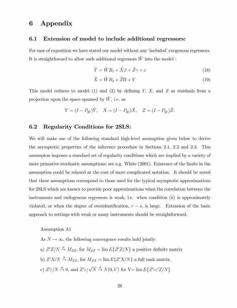
6.2 Regularity Conditions for 2SLS:

We will make use of the following standard high-level assumption given below to derive

the asymptotic properties of the inference procedure in Sections 2.1, 2.2 and 2.3. This

assumpton imposes a standard set of regularity conditions which are implied by a variety of

more primative stochastic assumptions; see e.g. White (2001). Existence of the limits in the

assumption could be relaxed at the cost of more complicated notation. It should be noted

that these assumptions correspond to those used for the typical asymptotic approximations

for 2SLS which are known to provide poor approximations when the correlation between the

instruments and endogenous regressors is weak, i.e. when condition (ii) is approximately

violated, or when the degree of overidentification, r − s, is large. Extension of the basic

approach to settings with weak or many instruments should be straightforward.

Assumption A1

As N →∞, the following convergence results hold jointly:

a) Z 0Z/Np→MZZ, for MZZ = limEZ 0Z/N a positive definite matrix

b) Z 0X/Np→MZZ, for MZX = limEZ 0X/N a full rank matrix.

c) Z 0ε/Np→ 0, and Z 0ε/

√N

d→ N(0, V ) for V= limEZ 0εε0Z/N

28

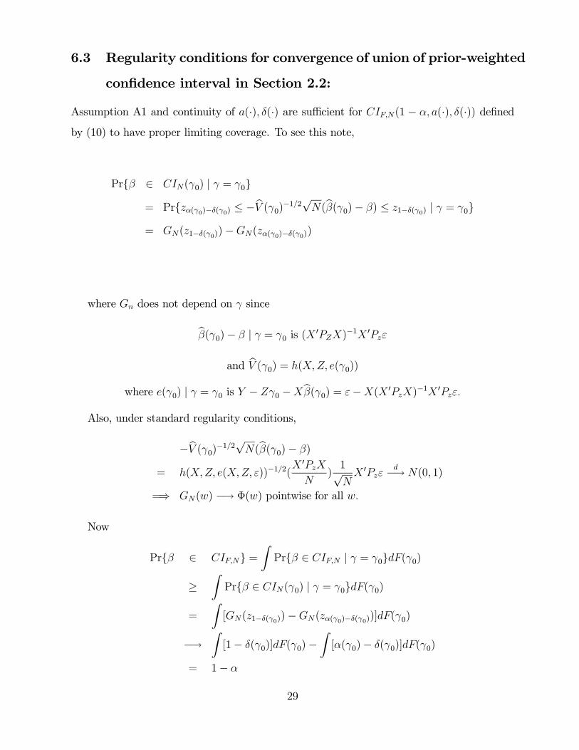
6.3 Regularity conditions for convergence of union of prior-weighted

confidence interval in Section 2.2:

Assumption A1 and continuity of a(·), δ(·) are sufficient for CIF,N(1 − α, a(·), δ(·)) defined

by (10) to have proper limiting coverage. To see this note,

Prβ ∈ CIN(γ0) | γ = γ0

= Przα(γ0)−δ(γ0) ≤ −bV (γ0)−1/2√N(bβ(γ0)− β) ≤ z1−δ(γ0) | γ = γ0

= GN(z1−δ(γ0))−GN(zα(γ0)−δ(γ0))

where Gn does not depend on γ since

bβ(γ0)− β | γ = γ0 is (X0PZX)

−1X 0Pzε

and bV (γ0) = h(X,Z, e(γ0))

where e(γ0) | γ = γ0 is Y − Zγ0 −Xbβ(γ0) = ε−X(X 0PzX)−1X 0Pzε.

Also, under standard regularity conditions,

−bV (γ0)−1/2√N(bβ(γ0)− β)

= h(X,Z, e(X,Z, ε))−1/2(X 0PzX

N)1√NX 0Pzε

d−→ N(0, 1)

=⇒ GN(w) −→ Φ(w) pointwise for all w.

Now

Prβ ∈ CIF,N =ZPrβ ∈ CIF,N | γ = γ0dF(γ0)

≥ZPrβ ∈ CIN(γ0) | γ = γ0dF(γ0)

=

Z[GN(z1−δ(γ0))−GN(zα(γ0)−δ(γ0))]dF(γ0)

−→Z[1− δ(γ0)]dF(γ0)−

Z[α(γ0)− δ(γ0)]dF(γ0)

= 1− α

29

where the first inequality follows because β ∈ CIN(γ0) | γ = γ0 impliesβ ∈ CIF,N | γ =

γ0; the interchange of the limit and integral follows from |GN(h(γ))dF | ≤ dF which is inte-

grable, α(·), δ(·) continuous, and convergence a.e; and the last equality fromRα(γ0)dF (γ0) =

α by construction.

6.4 Proof of proposition 1 in Section 2.3

The 2SLS estimator can be written as

βN = (X0PZX)

−1X 0PZY

Substitution of our model for Y yields:

βN = (X0PZX)

−1X 0PZX0β +

(X 0PZX)−1X 0PZZη/

√N + (X 0PZX)

−1X 0PZε

rearranging and scaling by√Nyeilds

√N³βN − β

´=h√

N(X 0PZX)−1X 0PZε

i+ (X 0PZX)

−1X 0PZZη

Assumption A1 implies that the term in brackets converges in distribution to¡M 0

ZXM−1ZZMZX

¢−1M 0

ZXM−1ZZv and the second term converges in distribution to¡

M 0ZXM

−1ZZMZX

¢−1M 0

ZXη.

6.5 Nonlinear Models

For ease of exposition, we considered each of the inference methods in the main text in

the context of the linear IV model. Linear IV models are a leading case in which to apply

our methods, but our basic results apply in any context in which there are unidentified

parameters and in which one may reasonably claim to have some sort of prior information

about their plausible values. The Bayesian approach discussed in Section 2.4 immediately

extends to nonlinear models, here we briefly discuss the extenstion to nonlinear models for

our other three approaches.

30

For concreteness, suppose that we are interested in performing inference about a para-

meter θ defined by as the optimizer of an objective function

hN(W ; θ, γ)

where W are the observed data, γ is an additional parameter, and θ and γ are not jointly

identified from the objective function but for a given value of γ, θ(γ) is identified. To

implement the bounds approach, we suppose that there is a true value for γ which is unknown

but is known to belong to a set G. We define

bθ(γ0) = argmaxθ

hN(W ; θ, γ0)

and suppose that√N(bθ(γ) − θ)

d→ N(0, V (γ)). That is, we assume that if we knew γ,

the estimator obtained by maximizing the objective function at that value of γ would be

consistent and asymptotically normal.12 Further suppose we have access to a consistent

estimator, bVN(γ0), of the asymptotic variance of bθ(γ0) under the hypothesis that γ0 = γ.

Then for each value of γ0 ∈ G, we may obtain an estimator bθ(γ0) and, under the maintainedhypothesis that γ0 = γ, construct a confidence interval analogous to (9) whose level might

depend on γ0 as

CI(1− a(γ0), γ0, δ(γ0)) = (bθ(γ0) + (bVN(γ0)/N)1/2cα−δ(γ0), (20)bθ(γ0) + (bVN(γ0)/N)1/2c1−δ(γ0)).Confidence intervals using the methods in Sections 2.1 and 2.2 can be directly constructed

by plugging (20) into expression (7) to obtain a union of confidence intervals utilizing only

the knowledge of the support of γ. Likewise, (20) can be plugged into expression (10) to

obtain a prior-weighted confidence interval which enables computaion of minimum length

prior-weighted interval via solution of (11).

For the local-to-zero approach in Section 2.3, we suppose that there are prior beliefs that

γ = γ∗ + η/√N where η ∼ G and η is indepenent of all other variables. In other words, we

assume that we know that γ is local to some value γ∗. As before, the normalization by√N

12This condition will be satisfied under the usual conditions for consistency and asymptotic normality of

M-estimators.

31

is best thought of as a thought experiment made to produce an asymptotic approximation in

which both uncertainty about the true value of γ and sampling error play a part. If we then

consider bθ(γ∗) as our point estimator we can obtain an approximation for the distribution ofbθ(γ∗) via the usual approach of linearizing first order conditions. Under regularity conditions√N(bθ(γ∗)− θ)

d→£−H(θ, γ∗)−1v

¤−H(θ, γ∗)−1J(θ, γ∗)η

where v is a normally distributed random variable, H(θ, γ∗) is the limit of ∂2hN (W ;θ,γ∗)∂θ∂γ0

and J(θ, γ∗) is the limit of ∂2hN (W ;θ,γ∗)∂θ∂γ0 . The term in brackets corresponds to the usual

limit distribution for bθ, the effect of uncertainty about exogeneity is to add in the term−H(θ, γ∗)−1J(θ, γ∗)η whose distribution of course depends on the prior G.

6.6 Discussion of MCMC Details

We outline our general strategy for full Bayesian inference for the model in (1) and (2). R

code to implement these samplers is available on request from the authors. Let Θ denote

the parameters of the error term distribution, i.e. the joint distribution of (εi, vi). In the

normal case, Θ = Σ is a covariance matrix. In an MCMC scheme, we alternate between

drawing the regression coefficients (β, γ,Π) and the error term parameters. A basic Gibbs

Sampler structure is given by

Θ|β, γ,Π, (X,Y,Z) (GS.1)

β, γ,Π| Θ, (X,Y,Z) (GS.2)

In the normal case, (GS.1) may be done as in Rossi et al (2005). The draw in (GS.2) is

accomplished by a set of two draws:

β, γ|Π, Θ, (X,Y,Z) (GS.2a)

Π|Θ, (X,Y,Z) (GS.2b)

Given Θ, we can standardize appropriately (by substracting the mean vector and pre-

multiplying by the inverse of the Cholesky root of Σ). The draws in (GS2.a) are then done

by realizing that, given Π, we "observe" vi and can compute the conditional distribution of

εi. Given (β, γ), the draw of Π is done by a restricted regression model. Rossi et al (2005,

chapter 7) provides details of these draws.

32

For the prior on gamma in (17), we cannot draw (β, γ) in one draw but must draw from

the appropriate conditionals.

γ|β,Π,Θ, (X,Y,Z) (GS.2a.1)

β|γ,Π,Θ, (X,Y,Z) (GS.2a.2)

We should note that for datasets with very weak instruments, the MCMC sampler defined

above can be highly autocorrelated, particularly for diffuse settings of the prior on γ. This

is not a problem if sufficient draws can be completed.

33

0 500 1000 1500 2000 2500 3000 3500 4000 4500 50005,000

0

5,000

10,000

15,000

20,000

25,000

30,000

35,000

δ

β

Figure 1: 95% Interval Estimates from 401(k) Example

Union of Symmetric CI

Minimum Length Union of CI

Bayesian

Local

Prior Weighted Union of CI

0 1000 2000 3000 4000 5000 6000 7000 8000 9000 10000−5000

0

5000

10000

15000

20000

δ

β

Figure 2: 95% Interval Estimates for 401(k) Example with Positive Prior

Union of CI

Local

Point Estimate

Bayesian

0 0.05 0.1 0.15−7

−6

−5

−4

−3

−2

−1

0

δ

β

Figure 3: 95% Interval Estimates from Margarine Example with γ|β Prior

Bayesian Local

Union of CI

0 0.001 0.002 0.003 0.004 0.005 0.006 0.007 0.008 0.009 0.01−0.2

−0.1

0

0.1

0.2

0.3

0.4

0.5Figure 4: 95% Interval Estimates from Returns to Schooling Example

δ

β

Union of CI

Local

Bayesian