1

Plato, and the Fractal Geometry of the Universe

Student Name: Nico Heidari Tari

Student Number: 430060

Supervisor: Harrie de Swart

Erasmus School of Philosophy

Erasmus University Rotterdam

Bachelor’s Thesis

June, 2018

2

Table of contents

Introduction ................................................................................................................................ 3

Section I: the Fibonacci Sequence ............................................................................................. 6

Section II: Definition of a Fractal ............................................................................................ 18

Section III: Fractals in the World ............................................................................................. 24

Section IV: Fractals in the Universe......................................................................................... 33

Section V: Fractal Cosmology ................................................................................................. 40

Section VI: Plato and Spinoza .................................................................................................. 56

Conclusion ................................................................................................................................ 62

List of References ..................................................................................................................... 66

3

Introduction

Ever since the dawn of humanity, people have wondered about the nature of the universe.

This was of course not very hard to initiate, our ancestors simply had to look up at the night

sky, and wonder what all those luminous dots in the sky where. But man is a curious beast,

and hence it did not stop there. The wise men of the past created myths, featuring many

different deities, which showed anthropomorphic characteristics and whose behavior could

explain the mechanics of the universe in an amusing manner. But at some point, philosophers

(literally “lovers of wisdom”) became unsatisfied over these narrations, and wanted to figure

out the true nature of the universe: its origin, size, evolution and fate. Little did they know,

what kind of immense project laid ahead of them.

How big is the universe? How was it made? What is it made out of? What kind of

shapes and rules govern its structure? This thesis aims to provide some elucidation on these

matters, in particular with the use of a new branch of mathematics called fractal geometry.

Geometry, as many may know, is the study of the properties of space, and shapes. It was first

thought that Euclidean geometry is the only type of geometry we can have. But in the 19th

century, by the work of many brilliant mathematicians, we came to the understanding that

other types can exist as well if we slightly change the classic axioms. Hence, hyperbolic and

elliptic geometry were born.

In addition, thanks to the work of some mathematicians such as Cantor, Peano, and

eventually Mandelbrot in the 20th century, another type of geometry was born: fractal

geometry. And it turns out that this type of geometry is extremely useful in describing and

simulating things in nature. The exact definition and nature of fractal geometry will be

explained in depth in the upcoming sections, because it is unfortunately too intricate to

explicate in a few introductory sentences. But, what I already can reveal to the reader, is that

it involves self-similarity and infinity.

But fractal geometry is much more than just another branch of mathematics. Its

applications are numerous, and thus it is an enormously interdisciplinary science. It eventually

encompasses many branches of mathematics, physics, astronomy, chemistry, cosmology, and

much more. I have attempted to provide a complete and thorough exploration of the most

relevant fields, in order to deeply understand this beautiful science. A rich understanding of it

will be useful when we start using it to discuss the nature of the universe.

4

Currently, fractal geometry is highly researched and very popular among scientists.

But it is still quite a young science and is still in the process of maturing. Benoit Mandelbrot

is considered the father of fractal geometry. In fact, he was not the first person working on

this new type of geometry, following Cantor, Riemann, Weierstrauss and other brilliant

mathematicians, but he was the person who grounded this study and gave it its own

vocabulary and grammar to work with. Accordingly, it has found applications in many fields

but there still has been relatively little research done on the significance of fractal geometry

with respect to cosmology, or the nature of our reality. This thesis aims to use fractal

geometry for these matters, in particular the nature and building blocks of the universe.

This is important because fractals have proved to be vital in the description of various

major components of the universe. There has been much empirical evidence that the universe

has a ‘fractal architecture’, i.e., that its big and small parts exhibit fractality. Philosophers

need to become aware and start theorizing about the implications of a universe with a fractal

architecture. What it indeed implies is that there exist a sort of simple, rule-governed structure

at the basis of all that exists. These ideas can be further extended to theorize the universe in its

entirety as a fractal, but more on this matter shall follow shortly.

When conducting this investigation, the researcher hypothesized that the universe

must be a fractal. The point of this research was to provide evidence that this was indeed the

case. It turns out that there are matters that complicate things, but more on that will be

discussed in due time.

Now, the structure of this thesis will be as follows. I start by describing and explaining

a very famous ratio of numbers in section I, called the golden ratio. Perhaps the reader is

already aware of the existence of such a ratio, since it has made many appearances in art, and

has been considered as ‘objectively’ beautiful by many. This golden ratio has a few

fascinating properties, and it seems to make appearances in all sorts of unexpected places in

mathematics, but also in nature.

This concept of the golden ratio will be used as a steppingstone towards the concept of

a fractal. Indeed, the golden ratio, when interpreted in a geometrical manner may be

considered as a proto-fractal. In Section II the rigorous definition of a fractal will be given and

explained, which has been provided by Mandelbrot. This requires familiarity with a number

of new concepts, which are vital when describing fractals. For example, the notion of

‘dimension’ has to be completely deconstructed, because the intuitive idea of dimension we

5

have will not suffice. But we will also see that the rigorous definition of a fractal is not

completely accurate, so instead we find a new way to conceptualize it, so that it can become

more useful.

After this, in Section III, we will venture in the world and see where fractals show up.

Many different examples will be explored in detail, so that the reader can gain an

understanding of the magnitude of these objects. We will start with an example from

mathematics, but quickly move on to nature, where we encounter many objects such as organs

or coastlines that exhibit self-similarity on many scales. In addition, there will be plentiful

illustrations to make the idea of self-similarity more clear.

In section IV we will consider some fractals on the astronomical scale, that of planets,

solar systems and galaxies. Astonishingly, these objects also exhibit fractality that is to be

found on much smaller scales. This part is in particular very important, because after this we

are going to discuss the possibility of the universe as a fractal. Since the biggest chunks of the

universe are galaxies, nebulae and gas clouds, it is important that this macroscopic objects

agree with the concept of a fractal.

Then, we will discuss in more detail the nature of the universe, with a fractal model in

Section V. This type of description of the universe with fractals is called ‘fractal cosmology’,

more on this later. In this part I first describe our current model of the universe, its shape and

what it is made out of. It turns out that there are many mysterious entities that are relevant for

these types of descriptions. Also, empirical evidence on the nature of the universe points

towards some very weird and unintuitive properties, but they must be seriously considered if

we want to have conclusive knowledge on the nature of the universe.

Lastly, in section VI, we reflect upon what we have learnt about fractals and think

about how it relates to some big ideas in history. In particular, I argue that major philosophers

like Plato and Spinoza were already aware of the presence of fractal patterns in the universe.

But they simply did not have the vocabulary yet to describe these matters accurately, since

this was not yet possible before Mandelbrot. Nonetheless, I noticed that they had a very

intuitive notion of a fractal, and I explicate some important ideas of their philosophies, in

order to show the similarities between their thinking and fractals.

6

Section I: The Fibonacci Sequence

Consider the following sequence of numbers

1, 1, 2, 3, 5, 8, 13, 21, 34, 55, 89, 144, 233, …

What is the pattern that underlies this collection of numbers? Clearly, it is as follows: one

takes the first two numbers (1 and 1), adds them together, and thus produces the third number

(1+1=2). Then, one takes the second and third number (1 and 2) and adds those together

(1+2=3). This step is repeated over and over again ad infinitum. We get 2+3=5, 3+5=8,

5+8=13, etc. This famous sequence is first considered by Leonardo of Pisa (nickname

“Fibonacci”) in 1202 (Hofstadter, 1980). One might wonder, so what? What is the

significance of this sequence of numbers? In fact, it has a few properties that illuminate some

of the most beautiful patterns in nature, a form of regularity and recursivity, whose existence

seems inexplicably mysterious.

To understand this fully we need to introduce some mathematical notation. The first

two terms are called the ‘seeds’ of the set, and the rules by which we generate new numbers

are called the ‘recursive relationships’ (Hofstadter, 1980). Thus, we can define the sequence

as follows:

𝐹𝐹𝑛𝑛+2 = 𝐹𝐹𝑛𝑛 + 𝐹𝐹𝑛𝑛+1 (1.1)

Hence, given the two base terms 𝐹𝐹0 and 𝐹𝐹1 (the axioms), we can calculate the next number in

the sequence, i.e. 𝐹𝐹2. If we want to know 𝐹𝐹3, we simply add 𝐹𝐹1 and 𝐹𝐹2 together as stated by

formula (1.1), and so on. Depending on what numbers we choose, the sequence will look

differently. Of course, if we pick 𝐹𝐹0 = 1 and 𝐹𝐹1 = 1, we get the famous Fibonacci Sequence.

However, if we change the base to 𝐹𝐹0 = 1 and 𝐹𝐹1 = 3 we get the Lucas Sequence:

1, 3, 4, 7, 11, 18, 29, 47, 76, 123, 199, …

Even though the numbers are different, the same principle of recursion is maintained.

Furthermore, in the Fibonacci sequence, something bizarre happens if for every n, we

divide 𝐹𝐹𝑛𝑛+1 by 𝐹𝐹𝑛𝑛, i.e., 𝐹𝐹𝑛𝑛+1𝐹𝐹𝑛𝑛

. Accordingly, in table A (Peitgen, Jürgens, & Saupe, 2006) I

elucidate the strange pattern that emerges after performing this computation.

7

Table A

n 𝐹𝐹𝑛𝑛 𝐹𝐹𝑛𝑛+1𝐹𝐹𝑛𝑛

Answer (to 6 decimal

places)

0 1 1/1 1

1 1 2/1 2

2 2 3/2 1.5

3 3 5/3 1.666666

4 5 8/5 1.6

5 8 13/8 1.625

6 13 21/13 1.615385

7 21 34/21 1.619048

8 34 55/34 1.617647

9 55 89/55 1.618182

10 89 144/89 1.617978

11 144 233/144 1.618056

12 233 377/233 1.618026

13 377 610/377 1.618037

14 610 987/610 1.618033

If we look at the numbers produced by the answer to the computation 𝐹𝐹𝑛𝑛+1𝐹𝐹𝑛𝑛

, we see that it

approaches some number, that is, it converges. To what does this converge? The answer is:

the golden ratio, or in more original terminology, the proportio divina (divine proportion).

The number

1.618033988749894848820458683436563…

is what we end up with if we perform the iteration 𝐹𝐹𝑛𝑛+1𝐹𝐹𝑛𝑛

for a very large n, say n = 1000.

A common convention to represent this special number within mathematics is by the

Greek letter 𝜏𝜏 (“tau”) or another Greek letter φ (“phi”). It does not really matter which one we

use, but for the remainder of this thesis, let us stick to φ, purely because I think that

aesthetically it is more appealing. Note that φ is an irrational number, meaning that it cannot

be written as 𝑝𝑝𝑞𝑞

, where p and q are integers. This can be proven by a reductio ad absurdum,

8

but we are going to omit the proof since that is quite lengthy and algebraic, and above all a bit

superfluous for my investigation. What is important to consider here, something that will

remain a recurrent theme throughout my thesis, is that as a consequence of this irrationality,

the number φ has an infinite decimal expansion.

Geometric Fibonacci

The reason it was called the “golden ratio” has to do with a more geometric conceptualization.

Euclid was the first to define the golden ratio in his influential book The Elements. He called

it the “extreme and mean ratio” and it is defined as follows. Consider the line AC which has a

point B on it as shown in diagram 1. It is stated to be cut in such a ratio when the ratio

between AC to AB is equal to AB to BC (Fitzpatrick, 2006). Now, let the length of AB be

arbitrarily set to 1 and let the length of AC be called x. Then, clearly the length of BC = x – 1.

We thus obtain the following equality with respect to the ratios of lengths.

𝑥𝑥1

= 1𝑥𝑥−1

. (1.2)

Diagram 1

Multiplying both sides by (x – 1) yields

𝑥𝑥2 − 𝑥𝑥 = 1 (1.3)

∴ 𝑥𝑥2 − 𝑥𝑥 − 1 = 0. (1.4)

Hence, using the quadratic formula (or ABC-formula), we obtain the following two roots:

𝑥𝑥1 = 1+ √52

and

𝑥𝑥2 = 1− √52

.

Clearly, the second (negative) root does not have any physical significance in this scenario.

But the positive root is the golden proportion we were looking for, i.e.,

A B C

9

1+ √52

= 𝜑𝜑.

Golden Ratio in Two Dimensions

The divine proportion makes an appearance in numerous geometrical shapes. Let us now

consider regular convex polygons. Regular convex polygons are figures that are equilateral,

but also equiangular in Euclidean geometry. Furthermore, all of its vertices are situated on a

common circle, which is called the circumscribed circle or circumcircle. Its interior angles

have a measure of (𝑛𝑛−2)𝜋𝜋𝑛𝑛

radians. This can simply be found by dividing the n-gon into

isosceles triangles, then adding up all the angles and subsequently dividing by the number of

angles it has. E.g., a regular pentagon can be easily cut up into three isosceles triangles. Since

the sum of the interior angles of a triangle equals 𝜋𝜋, it follows that the sum the interior angles

of three triangles is 3𝜋𝜋. Hence, each angle of the regular pentagon is 3𝜋𝜋5

radians, and we are

done (3𝜋𝜋5

radians = 108 degrees).

If we stick to the regular pentagon for now, it has another neat property, namely that

the ratio of the diagonals to its sides is once again the golden ratio. Proof: we consider the

regular pentagon ABCDE with AB = BC = CD = DE = AE = 1.

We connect vertex B with E and draw a line (which is one of the diagonals). Then, we drop a

perpendicular bisector from A, which bisects the angle A and falls on the midpoint of BE in

point G. Earlier it was proved that each angle of a regular pentagon is 108°. Hence, angle

∠BAG = ∠EAG = 54°. Furthermore, since AG was a perpendicular to BE, this means that

∠BGA = EGA = 90°. If we know two angles of a triangle we can calculate the third one,

yielding: ∠GBA = ∠GEA = 36°. Thus, by the postulate Angle-Angle-Angle, triangles BGA

B

C D

E

1

G

A

Figure 1

10

and EGA are congruent. Now, we can calculate the length of BG by using simple

trigonometry.

sin(∠𝐵𝐵𝐵𝐵𝐵𝐵) = 𝐵𝐵𝐵𝐵𝐵𝐵𝐵𝐵

sin(54°) = 𝐵𝐵𝐵𝐵1

sin(54°) = 𝐵𝐵𝐵𝐵

𝐵𝐵𝐵𝐵 = 0.809016994 …

Since BG = GE, that means that BE = 2BG. Thus,

𝐵𝐵𝐵𝐵 = 2 ∙ 0.809016994 …

= 1.618033989 …

= 𝜑𝜑

and in a similar fashion, it can be proven that diagonal CE = 𝜑𝜑. But to know for sure that

2 sin(54°) = 𝜑𝜑 exactly, and not just a number that is approximately equal, we need to prove

this as well. For this, consider figure 2 which shows an isosceles triangle ABC, with angles A

= 36°, B = 72° and C = 72°.1 If we bisect angle C as follows, we construct a triangle BCD

which is similar to triangle ABC. Since we have two isosceles triangles, we can fill in the

lengths of all the sides of the triangles as follows (with a’s and b’s), because if the base angles

of a triangle are equal, then their respective sides are also equal. Now, the sides of similar

triangles are proportional, meaning that all the corresponding sides will have a common ratio.

So, (AC/BC) = (BC/BD) = (a + b) / a = a / b. But this is simply the golden ratio from formula

(1.2)! The only thing we did in (1.2) is set the length of a arbitrarily to 1, which gives

1+𝑏𝑏1

= 1𝑏𝑏

(1.5)

∴ 𝑏𝑏2 + 𝑏𝑏 = 1 (1.6)

∴ 𝑏𝑏 = −12

+ 12 √5 (1.7)

1 Figure 2 and 3 are a courtesy of Kevin Knudson, 2015, October 29. Retrieved 2018, May 27 from https://www.forbes.com/sites/kevinknudson/2015/10/29/devilish-trigonometry-linking-the-number-of-the-beast-and-the-golden-ratio/#1682f8922c5d

11

∴ 𝑎𝑎 + 𝑏𝑏 = 1 − 12

+ 12 √5 (1.8)

= 12

+ 12√5

= 1+√52

= 𝜑𝜑

Now, for the final step we drop a perpendicular bisector from D to line segment AC. This

yields the following measurements.

Again, using simple trigonometry we find that

Figure 2

Figure 3

12

sin(54°) =𝑎𝑎+𝑏𝑏2𝑎𝑎

= 𝑎𝑎+𝑏𝑏2𝑎𝑎

.

But a + b = 𝜑𝜑 and a = 1, therefore,

sin(54°) = 𝜑𝜑2 .

Hence, 2 sin(54°) = 𝜑𝜑 exactly. We have now proven what we set out to prove in the

beginning, namely that the ratio of the diagonals to the sides of a regular pentagon is the

golden ratio. ∎

From the constructions in the pentagon, we obtain the so-called “golden gnomon” (in

the pentagon there are two) and “golden triangle” (this only occurs once in the middle, and of

course, this is the type of isosceles triangle we used to prove that 2 sin(54°) = 𝜑𝜑) (Dunlap,

2007, p. 15)2:

and these two special triangles have another interesting property. They can be dissected into

smaller, self-similar triangles. The left one will be dissected into smaller golden gnomons, and

the right one in smaller golden triangles. This is possible because of the relation of formula

(1.2), which after replacing x by 𝜑𝜑 and doing some algebra yields that

𝜑𝜑 − 1 = 1𝜑𝜑

. (1.9)

2 The images are retrieved from http://www.wikiwand.com/en/Golden_triangle_(mathematics)#/Golden_gnomon and https://commons.wikimedia.org/wiki/File:Golden_triangle.svg respectively.

1 1

𝜑𝜑

𝜑𝜑 𝜑𝜑

1

Figure 4

13

The dissection proceeds as follows, and is named “inflation” (indicated by the blue line).

Clearly, this inflation process may continue indefinitely, with each step producing more

golden gnomons and triangles. Each time this step is executed, the linear dimension of the

new triangle is reduced by a factor of 𝜑𝜑, and its area by 𝜑𝜑2. If we repeat this step numerous

times for the golden triangle, and connect the vertices of all the generated golden triangles

with an arc, we obtain the following image3.

Similarly, this process can be carried out for a “golden rectangle”. What is a golden

rectangle? It is a rectangle whose ratio of the longer side to the shorter side is the golden ratio.

In the same manner as with the triangles, we can initiate an inflation process where in every

step, the golden rectangle is divided into a square and another golden rectangle. Here, just as

3 Image is a courtesy of https://en.wikipedia.org/wiki/Golden_triangle_(mathematics)

1 1

𝜑𝜑

𝜑𝜑 𝜑𝜑

1

1 1/𝜑𝜑

1/𝜑𝜑

1

Figure 5

Figure 6

14

with the golden gnomons and triangle, the edges are reduced by a factor of 𝜑𝜑, and its area by

𝜑𝜑2. And again, we may connect the vertices (this time on the inside). This gives the following

image4.

The spirals that have been constructed by connecting the vertices of the golden triangle

and the golden rectangle are called the “logarithmic spiral”. The spiral can be drawn by

considering the point where the spiral converges to be origin of a polar coordinate system (r,

𝜃𝜃). A polar coordinate system is a different way to represent a point in a plane. Normally, we

would say that point is somewhere in the plane by denoting its distance from the x-axis and

the y-axis, which yields its respective x- and y-coordinates. With polar coordinates however,

we determine its point by saying how far it is from the origin (its distance or radius r), and

what angle it makes anticlockwise starting from the x-axis (as is the convention). This is

illustrated by figure 8.5 We end up with the description of the exact same point but in a

different manner.

4 Courtesy of https://commons.wikimedia.org/wiki/File:Fibonacci_spiral.svg 5 Retrieved from http://tutorial.math.lamar.edu/Classes/CalcII/PolarCoordinates.aspx

φ

1

1 1/φ

Figure 7

15

1 2

This makes it possible to plot circular curves with relative ease. For example, figure 96 shows

the picture we get for the function

𝑟𝑟(𝜃𝜃) = 1

where it does not matter what the angle 𝜃𝜃 is, the radius remains 1.

However, if we decide to create a function where the radius depends on the angle, then

we can start to get more interesting shapes. Figure 10 shows the so-called “Archimedean

spiral”7, which is described by the function

6 Pbroks13, 2008. Retrieved from: https://en.wikipedia.org/wiki/File:Circle_r%3D1.svg 7 Pbroks13, 2008. Retrieved from: https://en.wikipedia.org/wiki/File:Spiral_of_Archimedes.svg

Figure 8

Figure 9

16

2 1 3

𝑟𝑟(𝜃𝜃) = 𝜃𝜃2𝜋𝜋

, for 0 < 𝜃𝜃 < 6π.

Let us plug in some values and see if we can understand how this curve is made. Starting with

an angle of 6π yields

𝑟𝑟(6π ) = 6π 2𝜋𝜋

= 3.

If we look at figure 10, we indeed see that if we turn by an angle of 6π (i.e., three full

rotations) we end up at the point (3, 6π) or (3, 0) since they are the same point. The same goes

for

𝑟𝑟(5π ) = 5π 2𝜋𝜋

= 2.5

where we turn two and a half turns and end up on the left-hand side with a distance of 2.5 to

the origin. Clearly, for every incremental step we take, the radius drops slightly from 3, all the

way down to 0. And if we trace all the points that we get from this function, the image is

produced that we can see in figure 10.

Now, for the spiral in figure 7, we consider the diagonals of the golden rectangles as

illustrated in figure 11. 8 Here we see that the diagonal of the biggest rectangle falls at right

angles to the diagonal of the smaller one. Furthermore, both these diagonals are the diagonals

of each smaller rectangle in the process of inflation (Dunlap, 1997, especially p. 19).

8 Yearofthetulip, 2013. Retrieved from: https://commons.wikimedia.org/wiki/File:Golden_Ratio_4.jpg

Figure 10

17

Therefore, the rectangles will converge at the point of intersection of the diagonals. At that

point we imagine that our polar coordinate system begins, and we then draw the curve as a

function of 𝜃𝜃: the bigger the angle, the bigger the distance from the origin. Also, Euler’s

number is introduced to the formula, which is associated with natural growth, yielding the

formula

𝑟𝑟(𝜃𝜃) = 𝑝𝑝𝑒𝑒𝑞𝑞𝜃𝜃 (1.10)

where p and q are simply two constants.

Now, does this spiral look familiar? For me, the image that immediately comes to

mind is the shell of a gastropod (snail). Not only that, the Fibonacci spiral seems to make

appearances in all sorts of natural phenomena. Sticking to the example of the shell, there is an

animal called the Nautilus pompilius whose shell (in the form of a spiral) is built of

consecutive chambers. In fact, it turns out that the ratio between each consecutive chamber is

again the golden ratio (Dunlap 1997). To me it is absolutely astonishing to find φ in the

growing patterns of organisms.

But it does not stop there. There are countless examples of the golden ratio showing up

in nature. Another example is related to the growing patterns of plants. The arrangement by

which leaves are ordered on the stem of a plant is called phyllotaxis. With phyllotaxis, leaves

are usually ordered in a spiraling manner, and again the ratio between consecutive leaves have

the golden ratio. A few examples of manifestations of Fibonacci-based phyllotaxis are in

pineapples, oaks, hazels, Aloe polyphylla, and willows. A small digression: Kepler was the

first person to notice the recursivity of the Fibonacci sequence in phyllotaxis (Livio, 2008).

Figure 11

18

Section II: Definition of a Fractal

Mathematical Definition

The Fibonacci sequence is an appropriate way to make a transition to the next topic of this

thesis: fractals. So, what is a fractal? Alas, it is something which is not easily definable. There

are multiple ways to define it, but each of them is still not complete to grasp the infinitely rich

elegance of this mathematical object. But exactly for this reason it is a superb subject for

philosophical reflection. Note, I do not mean to suggest that I will in any way improve the

definition we have of fractals as of now. My only goal here is to explicate the concept of a

fractal to the reader, so that I may use this concept to argue my thesis: namely that the

universe has a fractal architecture, or exhibits ‘fractality’.

Let us start with the mathematical definition of the fractal. For this we turn to Benoit

Mandelbrot (1924-2010) who was a polymath, besides being a brilliant mathematician. He

made the biggest contribution to fractal geometry, and insisted that people would call him a

‘fractalist’. He even coined the term “fractal”, after the Latin frangere which means “to

break”. The reason for calling this thing “broken”, will become apparent soon, but for now it

is quite clear that if we want to define a fractal, this individual is the ultimate authority.

According to Mandelbrot (1983, p. 177) a fractal set (all the fractals that exist) is “a

mathematical set such that [the fractal dimension] D is greater than the topological dimension,

𝐷𝐷𝑇𝑇”. Now, to understand this definition, we need to first understand that there are also

multiple ways to define a dimension (and so the complicatedness begins!).

Dimension

The intuitive way to define the dimension of a (mathematical) object is to say that it is the

number of coordinates required to uniquely describe its points. This is further explicated by

Poincaré, who starts with a point which thus clearly has 0 dimensions, since it has no width,

breadth or height. Hence, a line has 1 dimension since it can be divided into two segments by

a point. Similarly, a square can be divided into two segments by a line, so it has 2 dimensions.

And lastly a cube has 3 dimensions, since it can be divided into two chunks by a square

(Peitgen, Jürgens & Saupe, 2006).

Furthermore, this notion of dimension is brought into topology, to yield the

topological dimension. Topology is a relatively new branch of mathematics. It looks at

notions of form and shape with a qualitative perspective (Peitgen et al., 2006). Objects (or

19

topological spaces) are perceived as invariant under certain transformations called

homeomorphisms. Examples of homeomorphisms are stretching, bending or crumpling. But

tearing or pasting objects are not allowed. More generally: holes are invariant, holes cannot be

added or subtracted without changing the object. So, for example, from a topological

perspective, a coffee mug and a donut are indistinguishably the same object, because if it is

made from stretchy material, one can be deformed into the other, and vice versa. The

topological dimension is then the dimension that does not change under such

homeomorphisms, e.g. a dodecahedron can be deformed into sphere, but its dimension will

remain 3 (Elert, 2003).

Monster Curves

In the end of the 19th century, mathematicians like Guiseppe Peano (1858-1932) and David

Hilbert (1862-1943) introduced some curves that destroyed this notion of a topologically

invariant dimension. Accordingly, these curves they had described were named “monsters”

(Peitgen et al., 2006). Peano introduced the following curve, named the Peano monster curve.

It is created as follows. We start with a regular square, and name it a cell. Then the first step is

to split the square up into four small copies that are exactly the same (see figure 12, ignore the

square in the middle for now). Next, the second step is to draw a line, starting at the edge of

one cell, and then tracing it through each cell to return to the initial point. The rules are that

the line can only go to adjacent cells (so it may not make any jumps) and that it may not cross

any cell twice. This line is then the Peano monster curve, and is illustrated in figure 12 (the

square in the middle of left-most cell, and in the cell immediately to the right, where the curve

looks like a capital I). Step 3 is to return to step 1, hence these steps are repeated ad infinitum.

The right-most cell is what we end up with if hypothetically iterated to infinity.

The reason this curve is called monstrous is because of the following. We started out

with a line, but since it is infinitely twisted and infinitely stretched out, it ends up visiting

every single point in the square! Thus, it becomes indistinguishable from a square, the curve

is now actually a square. But we went from a 1-dimensional object to a 2-dimensional object,

simply by stretching and bending the curve, which are homeomorphic transformations. This

Figure 12

20

destroys the earlier remark that topological dimensions should remain invariant among

homeomorphisms (Elert, 2003)9.

But this is not necessarily a problem. Mathematicians in the past were abhorred by

such ‘monstrous’ curves which seemed to contradict the traditional ideas of dimension and

topology. The solution for this difficulty is to consider these types of curves as special types

of objects, which have a topological dimension but also a so-called Hausdorff dimension

which is different from its topological dimension. The Hausdorff dimension is usually a

fraction, that is why it is also called a ‘fractal’ dimension by Mandelbrot (1983). This makes

sense if we consider the Peano monster curve again. It is made out of lines which have clearly

1-dimension, hence its topological dimension 𝐷𝐷𝑇𝑇 = 1 and remains 1. However, it exhibits

square-like behaviors in the end, so we can understand this and deduce that its Hausdorff

dimension must lie between 1 and 2 (the curve is somewhere between a line and a square).

Calculating the Hausdorff Dimension

Felix Hausdorff (1868-1942) conducted this groundbreaking work in the area of dimensions

and mathematics in 1919 (Peitgen et al., 2006). This type of dimension is applicable in all

(mathematical) objects that are self-similar. For example, a line is clearly self-similar, because

we can take said line, divide it into three equal parts which are all 1/3 of the length of the

original line. Then we can zoom in times 3 and we end up with the exact same line. This is the

notion of exact self-similarity. There are also other forms like quasi self-similarity and

statistical self-similarity, where the reduced-scaled images resemble the whole in some way

(Mandelbrot, 1967).

Now, there exists a law between the number of pieces n a self-similar object is cut

into, and the reduction factor f that was used, which is called the power law relation (Peitgen

et al., 2006) and is formulated as follows:

𝑛𝑛 = 1𝑓𝑓𝐷𝐷

(2.1)

where D = the objects dimension. So, for example, the line that was mentioned before which

was cut up in 3 equal parts yields

3 = 11/31

9 Figure 12 is retrieved from https://hypertextbook.com/chaos/topological/ and is attributed to (Elert, 2003).

21

which is correct. Furthermore, if we take a square which has two dimensions and cut it up into

9 equal smaller squares, we get

9 = 11/32

which is also clearly correct. The same principle can be applied to a cube. Now, if we only

know the scaling factor and the remaining number of pieces, we can use this information to

calculate its dimension D. For example, if we did not know the dimension of a square we

could compute the following calculation:

9 = 11/3𝐷𝐷

9 = 3𝐷𝐷

𝑙𝑙𝑙𝑙𝑙𝑙9 = 𝐷𝐷 ∙ 𝑙𝑙𝑙𝑙𝑙𝑙3

∴ 𝐷𝐷 = 𝑙𝑙𝑙𝑙𝑙𝑙9𝑙𝑙𝑙𝑙𝑙𝑙3

= 2 .

This is pretty straightforward. How about the Peano monster curve we encountered earlier?

We can use this power law relation to calculate its dimension. Consider figure 12 again. If we

look at the transformation that occurs when moving from the leftmost cell to the one adjacent

to its right, we see that 4 lines are transformed into 16. The corners of the lines do not matter

here, please consider a ‘line’ in this scenario as the line that goes from one side of the cell to

another. Then it clearly goes from 4 to 16. So, we are ready to do our calculation:

16 = 11/4𝐷𝐷

16 = 4𝐷𝐷

∴ 𝐷𝐷 = 𝑙𝑙𝑙𝑙𝑙𝑙16𝑙𝑙𝑙𝑙𝑙𝑙4

= 2

which gives a dimension of 2! This is then defined to be the Hausdorff or fractal dimension of

a curve. This is in agreement with our earlier speculation that since this is a space-filling

curve (i.e., it fills up all the points of a square), it must have a dimension of two. But this

conceptualization leaves the topological dimension intact. Its topological dimension is still 1

because it remains a line. But its Hausdorff or fractal dimension is 2 since the logarithm of

number of pieces divided by the logarithm of the scaling factor yields 2.

22

Note, that this space-filling curve is an exception to the rule: most fractal dimensions

yield a fraction as dimension (hence the name ‘fractal dimension’). But it still qualifies for

Mandelbrot’s definition of a fractal, since 2 > 1. Let us now consider a fractal that is more

general, say, the Koch snowflake. Its first four iterations are shown in figure 13.10

Consider the left edge of the first triangle. After the first iteration, this edge is replaced by 4

self-similar edges. But what is the scaling factor? Clearly it is 1/3, because if we put three of

these edges alongside each other, we obtain the original edge once again. This is clearly

illustrated by the green line in the middle of the edge of the first iteration. Then this step is

repeated again, but now on the left side there are 4 edges where this step needs to be iterated.

So another 4 little equilateral triangles are added with the bottom missing. Of course, since

this is a fractal this step is repeated to infinity, and we end up with a continuous curve without

any tangents. So what is then the fractal dimension? With each step the scaling factor is 1/3,

and the number of pieces we end up with is 4. This gives the calculation

𝐷𝐷 = 𝑙𝑙𝑙𝑙𝑙𝑙4𝑙𝑙𝑙𝑙𝑙𝑙3

= 1.261859507

10 Courtesy of https://commons.wikimedia.org/wiki/File:KochFlake.svg

Figure 13

23

which is a fraction! Just as expected. There exists also a very interesting fractal named the

Fibonnaci Word fractal (note the reappearance of the protagonist of section I) which has 𝐷𝐷 =

1.64 and 𝐷𝐷𝑇𝑇 = 1. This will be further investigated shortly.

Final Notes on the Definition

Now, returning to Mandelbrot’s definition of a fractal, it turns out that this definition is too

restrictive, because it excludes many fractals that are very useful in physics. For example,

clouds would not be accepted under this definition as a fractal, whilst fractal geometry has

proved very useful in determining their size and other elements. Thus, Mandelbrot changed

his mind and defined fractals as shapes whose parts are similar to the whole somehow (Feder,

2013). There is still quite some disagreement about the definition, but in general most

mathematicians agree that a fractal has the following characteristics: it is self-similar (exactly,

quasi or statistically similar), it has fine details at arbitrarily small scales, it is irregular in a

way that cannot be easily expressed in the vocabulary of Euclidean geometry (i.e., we require

the fractal dimension D), and lastly it is possibly recursive (Falconer, 2004). Therefore, we

can conclude that e.g. a square is not a fractal, even though it shows self-similarity, it does not

have fine details on minute scales, nor is it difficult to explain in Euclidean terms (it is simply

2-dimensional). In addition, it is also sometimes relevant that fractals are continuous, but

nowhere differentiable (Liu, Zhang & Yue, 2003), and moreover that some fractals have a

finite area, but an infinite circumference (e.g., the Koch snowflake).

24

Section III: Fractals in the World

Fractals in Mathematics

So, we have thus arrived at the section where we will take a journey into the world and see

where fractals show up. I hope the reader has somewhat of an intuition for these mysterious

objects as of now, but to recapitulate: a fractal is something that, when zoomed in, the parts

show some resemblance to the whole. The concept of recursion might also be helpful to grasp

its intricacy. Hofstadter (1980, p. 127) defines recursion as “nesting, and variations on

nesting”. What is important here, is that with recursion, there exist many different levels. And

on these various levels, the whole can be found in its parts with slight modifications.

According to Hofstadter, things like music and language can also embody recursion. Does

that mean that there exist linguistic fractals and melodic fractals? Perhaps, but that is beyond

the scope of this thesis to investigate. Instead, let us now start to examine an example of a

fractal within mathematics.

The non-trivial example that demands elucidation is the aforementioned Fibonacci

sequence! This might have already become obvious for the reader, because of the mentioning

of the Fibonacci Word Fractal, which is a fractal based on the Fibonacci word (which in turn

is based on the Fibonacci sequence, it seems like we have stumbled upon recursion in the

definition, a linguistic fractal perhaps?). The Fibonacci word is a particular sequence in the

binary alphabet of computers (zero’s and one’s) (Monnerot-Dumaine, 2009). This sequence is

formed by the same recursion pattern in formula (1.1), but instead of adding 𝐹𝐹𝑛𝑛 and 𝐹𝐹𝑛𝑛+1, we

simply put them next to each other (so we copy-paste 𝐹𝐹𝑛𝑛+1 behind 𝐹𝐹𝑛𝑛). Furthermore, the

initial ‘seed’ numbers are changed, with 𝐹𝐹1 = 1 and 𝐹𝐹2 = 0. So, the new recursion formula is

𝐹𝐹𝑛𝑛+2 = 𝐹𝐹𝑛𝑛+1𝐹𝐹𝑛𝑛 (3.1)

and the first nine iterations yields the following part of the infinite Fibonacci word.

Table B

𝑭𝑭𝒏𝒏 𝑶𝑶𝑶𝑶𝑶𝑶𝑶𝑶𝑶𝑶𝑶𝑶

𝑭𝑭𝟏𝟏 1

𝑭𝑭𝟐𝟐 0

𝑭𝑭𝟑𝟑 01

𝑭𝑭𝟒𝟒 010

25

𝑭𝑭𝟓𝟓 01001

𝑭𝑭𝟔𝟔 01001010

𝑭𝑭𝟕𝟕 0100101001001

𝑭𝑭𝟖𝟖 010010100100101001010

𝑭𝑭𝟗𝟗 0100101001001010010100100101001001

𝑭𝑭𝟏𝟏𝟏𝟏 0100101001001010010100100101001001010010100100101001010

The final Fibonacci word is the limit as n approaches infinity, i.e.,

lim𝑛𝑛→∞

𝐹𝐹𝑛𝑛.

Based on this Fibonacci word, an image is drawn with the following rules. We start

out by drawing one line segment forward. From hereon forward, every 0 we encounter in the

sequence means we have to take a turn: we turn left if its position in the decimal expansion is

even, and turn right if it is odd, and then draw a line. For example, the first 0 we encounter in

the sequence is also the first number in the sequence. Since it is the ‘1st’number, and 1 is an

odd number, we turn 90° to the right and then draw a line. Moreover, every time we encounter

a 1 in the sequence we simply draw a line in the direction we are moving. So e.g., the second

digit is a 1, so here we draw a line segment horizontally to the right (the direction we turned

after we encountered the first 0). The final step is to iterate these steps to infinity. Figure 14

shows the fractal from the 1st digit to the 14th.11 And figure 15 shows the image after 23

iterations.12

11 Prokofiev (2008, June 28) Retrieved from: https://commons.wikimedia.org/wiki/File:Fibonacci_fractal_first_iterations.png 12 Monnerot-Dumaine A. (2008, June 28) Retrieved from: https://commons.wikimedia.org/wiki/File:Fibonacci_fractal_F23_steps.png

26

Thence, an image is constructed which shows self-similarity on numerous scales with D =

1.637913. But even the spiral we found in figure 7 illustrates the fractalness of the Fibonacci

sequence. If one zooms in, a part of the spiral is similar to the original. Even the constructed

13 The calculation for this is 3 log𝜑𝜑

log(1+√2)

Figure 14

Figure 15

27

squares on a small scale resemble the totality. Hence, we find a beautiful recursion, i.e., a

nesting, of the whole in its parts.

Fractals in nature

The occurrence of fractals in nature is in essence innumerable, perhaps even infinite. In this

section I will discuss a number of them, those which I deem most significant. However, the

reader needs to keep in mind that this is merely a fraction of all possibilities that exist in

nature. But I hope that these examples will illuminate the fractal orientation of nature, so that

I may shortly legitimately deduce that the universe is a fractal.

The first interesting example to consider is the coastline of Great-Britain. A question

that puzzled geographers in the past is: what is the length of the coastline of Great-Britain? It

turns out, that the answer is: it depends! Or better yet: it is of infinite length. How so? For

that, imagine some person wants to measure it, and decides to do that by foot, with a

yardstick. Let the length of the yardstick be 𝜀𝜀, and the number of steps it takes S. Then,

clearly, if we multiply S with 𝜀𝜀, we will get the (approximate) length of the coastline, let us

call it 𝛬𝛬. Thus we have:

𝛬𝛬 = 𝑆𝑆 ∙ 𝜀𝜀 (3.2)

Sounds easy enough. But wait! If we make 𝜀𝜀 shorter, then new details of the coastline will

become measurable. Before, when walking across the coastline, the person who was

measuring it could not take a bunch of corners into consideration because his/her yardstick

was too long. But now it is shorter, so these missed corners can be included in the

measurement. Thus, say we take a quarter of 𝜀𝜀 and then suddenly 𝛬𝛬 (the length of the

coastline) is four times as long, i.e.

𝛬𝛬4 = 𝑆𝑆4 ∙𝜀𝜀4 (3.3)

It now becomes clear why it is difficult to measure the coastline of Great-Britain. Obviously,

we can repeat this reduction of scale an infinite amount of times, eventually generating:

lim𝑛𝑛→∞

(𝛬𝛬𝑛𝑛) = lim𝑛𝑛→∞

𝑆𝑆𝑛𝑛 ∙𝜀𝜀𝑛𝑛

. (3.4)

In plain English: if our yardstick is infinitesimally small, the length of the coastline will

become infinite, simply because there are an infinite amount of corners and details, that will

28

keep emerging if we continue to zoom in. Hence the conclusion: the length of this coastline

depends on the length of your yardstick.

It is due to reflection on these matters that Benoit Mandelbrot concluded that it would

be best to consider the coastline of GB as a fractal, and in that way approximate the actual

circumference. If we take into consideration the requirements put forward in section II, we

indeed find that this coastline (and in fact, every coastline) meets the necessary conditions,

namely that it is self-similar, it has new emerging details at arbitrarily small scales, and that it

is irreducible to Euclidean language (the fractal dimension calculated by Mandelbrot (1967)

for the west coast yielded D = 1.25).

Along a similar vein, vastly more natural phenomena have been discovered and

investigated as fractals. A cauliflower can be considered a fractal. A tree as well, and also a

mountain range. In fact, mountain ranges can very easily be simulated on the computer with

just a few simple instructions (with the help of fractal geometry of course) (Mandelbrot,

1983). The sky is also a fractal. So is a flower or a leaf. The same goes for snowflakes, which

are infinitely varied and complex. Even when I rub my eyes, I see fractal patterns emerging,

infinitely detailed, self-similar images. Could this perhaps mean that the secrets of human

nature are hidden somewhere in the language of fractal geometry? As a matter of fact, that

would not be farfetched at all!

The Fractal Brain

Liu, Zhang and Yue (2003) used fractal geometry to study the human cerebellum (CB). The

CB is located in the upper part of the hindbrain (above ones brainstem, near the back of ones

skull), and it plays a significant part in motor control and motor learning. It is also suspected

to play a role in a number of cognitive functions like language, attention, responses to fear,

etcetera. We share this part of the brain with all the vertebrates. The researchers measured the

“morphometric complexity” (by this they simply mean the fractal dimension D) and found

that indeed, the CB has a fractal architecture, with 𝐷𝐷 = 2.57 ± 0.01.

Other researchers have done studies on the fractal dimension of the brain as well.

Bullmore et al. (1994) investigated the complexities of the borderline between gray matter

and white matter with the help of MRI scans. They found that schizophrenic patients have a

lower fractal dimension of the brain than the control group, and that manic-depressive patients

have a higher fractal dimension than the control group. Blanton et al. (2001) found age related

differences in fractal dimension of the frontal parts of the brain. Kedzia, Rybaczuk and

29

Andrzejak (2002) can confirm age related differences, since they found that blood vessels of

the brain have 𝐷𝐷 = 1.26 during the fourth month of the fetal period, which increases to 𝐷𝐷 =

1.6 in the seventh month. It seems that if we consider the brain as a fractal, and all the

intricate networks that support it as well as fractals, that we can obtain deep insights into the

its mysterious workings. The fractal dimension is even a helpful tool to detect psychological

pathologies. I wonder what the fractal dimension was of Einstein’s brain, does the reader

think it was bigger than an average person, or smaller? Or perhaps it plays no roll at all in

intelligence. Hopefully, some future research will elucidate this matter.

The Fractal Building Blocks of the Human

It is clear now that the organization of the brain has a fractal dimension to it. But of course,

this does not yet mean that we have unlocked the secrets of human nature. Many philosophers

have argued that we are not just our brains. And I agree, because if that were the case, we

would just be a bunch of floating brains. There is another significant aspect to the human

nature, and that is the body. What is the human body made out of? Looking at the biggest

components of a human body, we find organs (the heart, the brain, the stomach, etc.) with

various distinct functions. And the backbone which holds this structure together is the

skeleton. Okay, but what are organs and bones made out of? They are made out of tissue. And

tissue, in turn, is simply a collection of cells. Cells are the building blocks of our bodies

(Schadé, 1987). But then another question arises, how are cells made?

For this we turn to deoxyribonucleic acid, colloquially known as DNA. Usually, DNA

is situated in the center of each cell, called the nucleus. DNA itself is made of molecules

called nucleotides. A number of these nucleotides are strung together, creating one strand of

DNA. But usually, when we encounter DNA, it comes in a double strand. Now, DNA is in

principle a blueprint of how to build enzymes (Hofstadter, 1980). Enzymes are bigger

molecular structures that serve as a catalyst to facilitate chemical reactions, and are essential

for life (human and non-human). Furthermore, enzymes are made by ribosomes in the

cytoplasm, which is the outside part of cell, excluding the nucleus. But now a difficulty arises,

the DNA is like a recluse who sits comfortably in his house, refusing to ever go outside and

interact with the world. How does information from the DNA reach the ribosomes?

This is the job of the messenger ribonucleic acid (mRNA). This strand of mRNA

carries information from DNA in the nucleus, to the ribosomes in the cytoplasm. The

information is copied by an enzyme in the nucleus from the DNA to the mRNA. This process

30

is called transcription (Hofstadter, 1980). Now, the enzymes that are made by the ribosomes

are part of the general category of proteins. Ribosomes are the manufacturers of all the

proteins in our body, including the enzymes. Proteins are made out of amino acids, which are

molecules similar in complexity as the nucleotide, thus serving as the building block of a

protein. But in this intricate process of creating a protein something extraordinary happens. As

the protein is created, it elongates, but also keeps folding itself into a sort of 3-dimensional

shape, called its tertiary structure. It is still a complete mystery in biology to figure out how

one can predict what the tertiary structure will look like, by looking at the sequencing of its

amino acids (which is the primary structure). When it goes from primary structure to the

secondary structure, the strings of amino acids form structures such as helices, sheets or loops.

Then, these structures interact with each other in many intricate ways to form the 3-

dimensional tertiary structure.

And this is exactly where fractal geometry becomes relevant again. It is my suggestion

that this mystery could perhaps be solved sooner if we consider the tertiary structure of a

protein as a fractal, which is generated by simpler geometric shapes (the amino acids). A

simplified version is illustrated in figure 16.14

Instead of thinking that the 2-dimensional shape somehow magically folds into a 3-

dimensional shape, it makes much more sense to consider the dimension of the protein as a

continuum, where it continuously moves from 2 to 2.0001, to 2.0002, etcetera until its final

shape. Of course, my suggestion at this point is merely a conjecture, but there is some

evidence to confirm that this supposition is headed in the right direction.

Enright and Leitner (2005) did a research on the fractal dimension of 200 proteins with

ranges of 100 to more than 10.000 amino acids. The average fractal dimension they found was

14 Holehouse, A.S., Garai, K., Lyle, N., Vitalis, A., and Pappu, R.V. (2015). Retrieved from: http://holehouse.org/pages/backbone_sidechains.html

Figure 16

31

D = 2.5, which is not at all the 3-dimensional shape that one would expect. They also found

that in general, D is bigger for bigger proteins (which contain more than 1000 amino acids),

i.e., 𝐷𝐷 ≈ 2.6, and that it is lower for smaller proteins (with around 100 amino acids), i.e., 𝐷𝐷 ≈

2.3. Furthermore, the researchers found that proteins are not compact objects that are

completely filled, but rather also have hollow areas. This also confirms the assertion that the

final dimension of a protein is less than D = 3. So there we have it: it makes much more sense

to consider proteins (which are fundamental building blocks of our bodies) as fractals, instead

of simple 3-dimensional structures.

From Building Blocks to Buildings

So, the DNA instructs the ribosomes how to construct proteins, which are fundamental

components of organisms and participate in almost all cellular processes. With the help of

these proteins, cells go on to build tissue and eventually organs and the like. Some organs

exhibit fractal-like structures or patterns, and these are definitely worth some consideration.

Havlin et al. (1995) expound that lungs exhibit forms and structures that are

characteristic of fractals. They say that the mammalian lung shows self-similarity at many

different scales. All the branches branch of into tinier branches, which all resemble the whole

somehow. This is similar to how a tree branches off into self-similar pieces, and there are

many tree-like fractals made in the past century, e.g. figure 17.15

Furthermore, the surface area of the lungs is enormous, which is something one would expect

from a fractal, in contrast to a regular compact object. Havlin et al. (1995) state that the area

15 Retrieved from: https://www.contextfreeart.org/gallery/view.php?id=3384

Figure 17

32

of human lungs is comparable to the size of a tennis court. In figure 18 we find an image of

the lungs which shows fractal-like patterns that resemble the branching of a tree16.

Moreover, Havlin et al. (1995) add another example of the human anatomy that has

fractal properties. This second example is the system of arteries. Arteries are responsible for

bringing nutrients and oxygen to every single cell in the body. This is of course an immensely

intricate procedure. Luckily, blood vessels branch off into very small pieces, with some

branches only measuring 5 micrometers! Eventually, after all the branching off, all the cells

can be reached. Also, the smaller copies of the vessels show a power-law distribution (see

formula (2.1)), similar to the one of (2.1), which can be found in most fractals. Lastly,

Sernetz, Wübbeke and Wlczek (1992) studied the arteries of kidneys, and found a fractal

dimension in-between 2 and 2.5. Figure 19 shows an image of blood vessels, which clearly

show fractal-like patterns17.

16 Henning Winter, 2015, September 1. Retrieved from: http://themagichappensnow.com/the-fractal-life/ 17 2013, December 3. Retrieved from: https://blogs.uoregon.edu/artofnature/2013/12/03/fractal-of-the-week-blood-vessels/

Figure 18

Figure 19

33

Section IV: Fractals in the Universe

Effective Dimension and Scaling

So far, the notion of a fractal has been elucidated, and examples have been given on how

some are formed. Moreover, we have ventured into the world to see where fractals show up.

However, as we all know, the universe is vastly larger than just planet Earth. In this section

we will consider some fractals that occur on bigger scales.

One of the things that has puzzled astronomers, mathematicians and (astro-)physicists

for many centuries is the distribution of galaxy clusters, galaxies and stars. The distribution

seems to be irregular and hierarchized, and no one as of yet seems to have explained why this

happens (Mandelbrot, 1983). To be able to describe these celestial structures in the

vocabulary of fractal geometry, we must introduce a new concept: the effective dimension.

Mandelbrot (1983, especially p. 17) expounds that this concept should be considered more

intuitively, instead of being defined rigorously.

Effective dimension is what physicists use to describe 3-dimensional objects which are

practically the same lower-dimensional mathematical constructs. For example, a ball made

out of threads seen from far away looks 0-dimensional, i.e. as a point. It is thus ‘in effect’ zero

dimensions. Of course in reality it is 3-dimensional but its effective dimension is 0. If we

zoom in, the ball shows spherical properties once again and has an effective dimension of 3.

But if we keep zooming in until the focus is on one fiber, the ball then has an effective

dimension of 1. Lastly, we could continue to zoom in until we are left with atoms which look

like points and hence have an effective dimension of zero. So the same object can have

different effective dimensions based on the scale it is being scrutinized. Obviously this is a

subjective notion. A novel addition by Mandelbrot is that he allows fractional dimensions for

this effective dimension. And, a little side note: Blaise Pascal (1623-1662) once claimed that

our world looks like a point from a galactic point of view.

Thus, when doing fractal geometry on physical bodies and structures of the universe, it

matters on what scale we (subjectively) choose to examine it. It has been a subject matter of

much controversy to unambiguously determine what the cutoff points are where it makes

sense to talk about a region of space and measure the fractal dimension D, where 0 < D < 3

(Mandelbrot, 1983, especially p. 86). But, no matter what the cutoff points are, the universe

embodies many different effective dimensions. When looking at the scale of planets we see 3

34

dimensions (since they are spherical objects with fine details). When zooming out far enough,

these celestial bodies look like 0-dimensional points.

Star Formation

Star formation is a branch of astronomy which studies how such celestial bodies are formed.

The place where protostars are formed are called the interstellar medium (ISM) and molecular

clouds. ISM is the substance and radiation that exists in-between star systems. A star system

is simply a collection of stars that exhibit gravitational attraction in each other’s vicinity. Most

of the elements found in such a region are helium and hydrogen (Herbst, 1995). And so, in the

densest areas of the ISM, stellar objects are formed in molecular clouds. ‘Molecular cloud’

does not need much elucidation, the name explains most of this entity, it is simply a cloud

between stars that is big and dense enough for molecules to form. In areas where huge

densities of gas and dust are located (these are called clumps), early stellar objects are made.

So, what does star formation have to do with fractals? In fact, it turns out that the gas

clouds in the ISM that create these stars are fractals themselves! This interesting insight was

found by Combes (2000) who found that the clouds in the ISM were hierarchized and showed

self-similarity on six orders of magnitude. Note that the self-similarity found in these levels of

gas clouds is statistical, instead of exact self-similarity (which is difficult to find outside of

mathematics). But of course, this is fine since the definition of Mandelbrot we saw earlier

allows statistical self-similarity. Furthermore, he found a fractal dimension of D ≈ 1.7, and he

also found the highest cut-off point where such fractals may exist. These occur in Giant

Molecular Clouds (GMC) which have a diameter of arounds 100 parsecs (a parsec is a unit to

measure astronomical lengths, one parsec is equal to approximately 3.26 light-years, or 30

trillion km) and a mass of 106 M (M is the symbol for “solar mass”. One solar mass is the

weight of our sun, and it is approximately 2×1030 kilograms. Similar to the parsec, this is a

common way to measure proportions of celestial objects). Lastly, these clouds exhibit a

power-law relation (similar to the one in section II, formula (2.1), which is a characteristic of

fractals). This one relates the cloud’s size R, velocity dispersion σ and mass M. Velocity

dispersion is a term in astronomy which takes a look at a group of objects (like a galaxy

(cluster)) and calculates the statistical dispersal of velocities around the mean of the entire

group. He obtained the following power laws (note, ∝ means “is proportional to”, so if the

left-hand side goes up, the right goes up as well. Similarly, if left goes down, the right goes

down too):

35

𝜎𝜎 ∝ 𝑅𝑅𝑞𝑞 (4.1)

where q is a constant that is estimated to lie between 0.3 and 0.5. And

𝑀𝑀 ∝ 𝑅𝑅𝐷𝐷 (4.2)

where D is of course the Hausdorff or fractal dimension. Personally, I find it fascinating to

find such elegant formulas of fractal geometry in such massive structures that occur in the

universe. Benoit Mandelbrot’s book “The fractal geometry of nature” already expounds in

great detail all the marvelous fractal structures there exist in nature (hence the title). But

nature is a very broad term and must include the universe as well. Kant once said that nature

is “the sum total of all appearances” (Rohlf, 2016), which is a neat way to conceptualize the

universe. So, gas clouds exhibit fractal properties or fractality, but they are not the only

massive objects in the universe that exhibit fractal properties.

Fractal Galaxies

Mandelbrot (1983) stated that on the right scale, galaxies show self-similarity and thus exhibit

fractality, with a fractal dimension that can be estimated by observational data. In the years

following this, researchers got inspired and went on to study galaxies and their respective

densities and dispersions to find a fractal dimension, so they could build evidence for the

claim that galaxies are fractals. Combes (2000) found a similar fractal dimension for galaxies

as for the ISM, i.e. D ≈ 1.7. Again, a similar power-law relation was found, and moreover it

has been proved that galaxies tend to hierarchize instead of having a homogenous distribution

in the heavens (this was already confirmed a while back, for example by Abell (1958)). This

hierarchization simply means that galaxies group together, form clusters, which in turn form

superclusters etcetera (to infinity?). All these characteristics of galaxies which coincide with

properties of fractals make it appropriate to conceptualize galaxies as fractals.

Furthermore it is noteworthy to examine at what type of scales it is possible to

consider galaxies as fractal structures. The smallest galaxies that exist function as the smallest

cut-off point where galactical fractal geometry is possible. These galaxies can be measured by

a scale of 10 kiloparsecs (1 kiloparsec = 1.000 parsecs) and their respective masses are

approximately 1010 M. (Combes, 2000, especially p. 15). These are then named “dwarf

galaxies”. But the higher cut-off scale has been subject to much controversy. There exists

quite some debate if this upper scale even exists. The definite answer to this debate can be

given by finding definite evidence that at a certain scale these fractal structures transition into

36

something homogenous and isotropic. This is the theory of the Cosmological Principle, which

states that matter is distributed throughout the universe in a homogenous and isotropic

manner, when viewed on a large enough scale. Homogenous means that the universe looks

the same from everywhere, i.e., it has no preferred origin (imagine a 2-dimensional Cartesian

coordinate plane which stretches out to infinity, but then without the axes. This is what is

meant here, but then in 3 dimensions! Or perhaps a fractional dimension between 2 and 3?)

Isotropic means that there does not exist a preferred direction (again think of the coordinate

system, there is no preferred ‘up’ or ‘down’). The strongest evidence found so far that favors

the Cosmological Principle is cosmic microwave background (CMB). What this concept

entails is explicated in section V, which deals with fractal cosmology. The aim of this

paragraph is to provide and explicate examples of fractals at the cosmic scale. But for now, if

the Cosmological Principle is correct, then it means that there is a cut-off point at the biggest

superclusters. These superclusters of galaxies are measured in scale by megaparsecs (which is

1.000 kiloparsecs or 1.000.000 parsecs). The biggest cut-off point would be at 300

megaparsecs according to Combes (2000), and these supercluster have a mass of around 1017

M.

For the remainder of this section I would like to show illustrations and explain some

galactic structures that exhibit beautiful fractal patterns. Studying fractals is not only about

studying abstruse mathematical formulas. It is also about visualizing them, noticing patterns,

and seeing how such fractals relate to things we find in the external world. Until now, fractal

geometry appears to be the type of geometry that is most accurate in describing complicated

objects and structures in nature.

Let us start with the most familiar galactic fractal, which is the one we live in: the

Milky Way galaxy. Actually, the etymology of the word “galaxy” derives from the Greek

word γαλαξίας (“galaxias”), which means “milky”. This is because in ancient times, a part of

the Milky Way was visible in the night sky, and people named it “milky circle”, because that

is what it looks like with the naked eye. The luminosity of the myriad of stars formed a milky

band, where the individual stars could not be distinguished. Now, the Milky Way is a so-

called “spiral galaxy”. This name is according to Hubble’s classification of galaxies, which he

made in 1926. Spiral galaxy is one of the three classifications of galaxies, the other two being

elliptical and lenticular galaxies (Hubble, 1926). Spiral galaxies are described by a bulky

center with a big collection of stars, known as “the bulge”. Outside of the bulge, there is a

37

disk with dust, gas and more stellar bodies. Lastly, they have spiral arms extending from the

center far into the galaxy, and these are active sites where new stars are born.

However, the Milky Way is a special type of spiral galaxy, called a barred spiral

galaxy. These types contain a bar in the center instead of a normal spiral, and have two

dominant arms (Redd, 2015). Figure 20 is an image of our (stunning) galaxy.18

Note, that we see a similar logarithmic spiral in the Milky Way as the one of section I where

we investigated the Fibonacci sequence. Moreover, the fractality of this galaxy is also due to

the distribution of disconnected dots (the stars) that are scattered everywhere. A collection of

disconnected dots is a fractal because it is in-between a dot and a line, so intuitively we can

already say that its Hausdorff dimension will lie between 0 and 1. This idea was introduced by

Georg Cantor in 1883, where he introduced the Cantor set, which is a collection of points but

constructed in an unique way. Eventually it was measured that this set (which we nowadays

call a fractal) had a fractal dimension19 D = 0.6309. The Milky Way is a structure that shows

statistical self-similarity on multiple scales, shows newly emerging details when zooming in,

and has a shape that requires the fractal dimension D, hence it is a fractal.

The closest galaxy to the Milky Way is called the Andromeda Galaxy, and is another

spiral galaxy. But this one is not “barred” so it does not have two major arms or a bar in the

center. Instead its center is more disk-shaped and it has no dominating major arms. The

Andromeda Galaxy has a span of around 220.000 light years, its distance from the Milky Way

is about 780 kiloparsecs, and it contains approximately 1012 stars. Figure 21 shows the

Andromeda Galaxy.20

18 Retrieved (2018, April 30) from: http://www.milkywaystars.com/ 19 Calculation is: log2

log3

20 Astro Bob (2017, January 25). Retrieved from: http://astrobob.areavoices.com/tag/andromeda-galaxy/

Figure 20

38

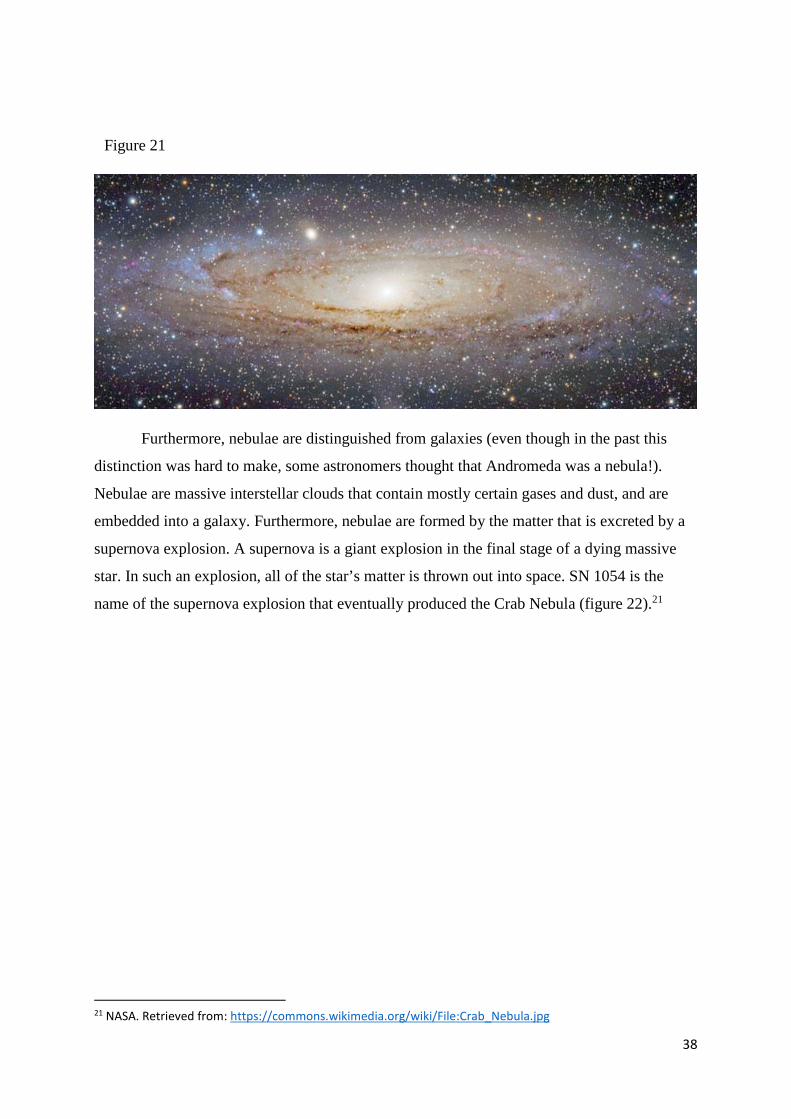
Furthermore, nebulae are distinguished from galaxies (even though in the past this

distinction was hard to make, some astronomers thought that Andromeda was a nebula!).

Nebulae are massive interstellar clouds that contain mostly certain gases and dust, and are

embedded into a galaxy. Furthermore, nebulae are formed by the matter that is excreted by a

supernova explosion. A supernova is a giant explosion in the final stage of a dying massive

star. In such an explosion, all of the star’s matter is thrown out into space. SN 1054 is the

name of the supernova explosion that eventually produced the Crab Nebula (figure 22).21

21 NASA. Retrieved from: https://commons.wikimedia.org/wiki/File:Crab_Nebula.jpg

Figure 21

39

This image is similar to a (slightly more complicated) dendrite Julia fractal which looks

something like figure 23.22

22 IkamusumeFan. Retrieved (2018, April 30) from: https://commons.wikimedia.org/wiki/File:Julia_0_0.8.png

Figure 22

Figure 23

40

Section V: Fractal Cosmology

So far, I have explicated the essence of fractals, and most of the abstruse concepts of

mathematics and physics that are needed to understand this wonderful phenomenon. Now we

are going to use those concepts and delve deep into the realm of quantum mechanics, and in

other interesting parts of the cosmos, to understand what fractal cosmology is all about.

So what is cosmology to start with? The layman can perhaps confuse this with

astronomy. What is exactly the difference? Well, astronomy studies objects or bodies that are

to be found in the observable universe. It studies how they are made and develop during their

‘lifetime’. Some examples include: galaxies, asteroids and stars. Cosmology actually also

studies these objects from time to time, but it is much more than that. It studies the universe in

general. It studies the origin of the universe (of course the most explicative theory we have

right now is the Big-Bang Model), how it evolves, and what the underlying laws are that

govern its structure. Dickau (2009) explains that cosmologists study the universe on the scale

of megaparsecs, but also on the smallest scales where the rules of quantum mechanics loom

large. So it is not only about planets and galaxies! It is also about electrons, quarks, muons,

and so on.

Fractal cosmology then, is a theory which attempts to understand and explain the

universe on the basis of fractals. Dickau (2009) states that cosmologists have already found

fractal-like structures on all imaginable scales. This is also quite obvious from some of the

fractals we encountered earlier. Of course, the galaxy serves as an example for a fractal on the

macroscale, where the unit of measurements are parsecs. We also encountered trees, clouds

and similar figures on what may be called the mesoscale. Lastly, one can think of snowflakes

on the microscale. It would be a rather implausible coincidence if the universe exhibits

fractality in many of its constituent parts completely at random. I believe this is a clear

argument in favor of the universe possessing fractal laws in its underlying structure.

Infinite Universe?

But what is the size of the universe? If this question was asked to a random individual on the

street, the answer might be “infinite”, or “very big”. But there is an important distinction here.

“very big” is finite, whilst infinite implies that there is no end. So which one is it? Is it

possible to ever know for sure?

41

That is hard to say, but there have been debates amongst cosmologists for quite a

while now on this matter. In particular there were discussions going on between Giordano

Bruno (1548-1600) and Johannes Keppler (1571-1630) on this matter. Bruno noticed the

similarity between the sun and other stars, and hence postulated that the night sky displayed

an infinitude of stars. This is further expounded in his book “About Infinity, Universe and

Worlds”, where he also postulates the universality of natural laws, besides stating that the

universe is infinite (Baryshev & Teerikorpi, 2002). Keppler, on the other hand, insisted that

the universe is still finite and that the stars are situated in the outside areas of our universe.

Clearly, the size of the universe has been subject to much controversy. What is the model that

we have of it now?

The Big Bang

In the 20th century there were debates going on between two models: the Big Bang and the

Steady State Theory. The Steady State theory follows the Perfect Cosmological Principle,

which states that the universe is homogenous (no preferred origin) and isotropic (no preferred

direction, up or down) in both space and time. However, empirical evidence has shown that

the universe has a finite age, i.e., it was created at some point around 14 billion years ago.

This means that it cannot have been homogeneous and/or isotropic forever, because at some

point it did not even exist! Therefore, the Steady State Theory has fallen short with the

explanation of certain empirical phenomena, so it cannot be true as a cosmological model. So,

the best model we have at this point is the Big Bang model, which follows the Cosmological

Principle, which only states that the universe is homogeneous and isotropic in space, not in

time.

I would also like to add two examples of the empirical evidence that has been found in

favor of the Big Bang model. The first one is so-called cosmological redshift (Wright, 2009),

which is related to the Doppler effect. The Doppler effect can be envisioned as follows.

Imagine sitting one day in your car in traffic. Suddenly, you hear a siren wailing in the

distance, an ambulance needs to go by! The cars move to the side and the ambulance can go

by with relative ease, and high speed. But while this happens you notice something. The

sound of the siren sounds different when it is approaching you, and it changes once it is

moving away. This is due to the Doppler effect. Of course, the sounds you are hearing are

simply soundwaves, which are channeled through the ear to deliver a message to the brain.

But when the ambulance is moving towards you, the soundwaves are compressed, making the

periodicity or frequency shorter. Imagine a sine wave with a period of 2π, but then

42

compressed to give a period of π. That is in essence what happens. On the other hand, when

the ambulance is moving away from you, the sound waves are stretched out by the movement

of the vehicle. The periodicity is now elongated, changing from say, 2π to 4π. Since the

soundwaves that reach the ear are completely different, the sound you will hear in this

situation will change accordingly.

Now the significance of this effect in cosmology becomes apparent when we consider

the visible light from distant galaxies. It has been proven that light behaves sometimes as a

particle and sometime as a wave. This has been theorized by brilliant physicists like Albert

Einstein (1879-1955) and Max Planck (1858-1947). Also, it has been confirmed with

scientific experiments such as the very famous double-slit experiment, which was first

performed in 1909 with light, but then repeated with other quantum particles as well such as

electrons. Nowadays, it is commonly accepted that all particles also possess a wavelength,

and this is called the wave-particle duality.

Hence, since light has wavelengths as well just like sound, the Doppler effect can be

used to study the light emitted from distant galaxies. Astronomers have found that the

wavelength from objects in deep space are overarchingly ‘redshifted’ (Baryshev &

Teerikorpi, 2002). Redshifted means that the spectral lines from the light are stretched out,

making its wavelength longer. Blueshift is the exact opposite, namely that wavelengths are

shortened, moving to the blue spectrum of visible light. But remember that shortened

wavelengths mean that the objects are moving towards us, elongated ones mean they are

moving way. But almost all distant galaxies seem to be moving away from us! The

observational evidence eventually led to Hubble’s law, which states that redshift increases as

distance increases from the observer to the object, or in more mathematical notation:

𝑣𝑣 = 𝐻𝐻 ∙ 𝐷𝐷 (5.1)

where v is the apparent velocity (calculated using the redshift), H is a constant of

proportionality called the “Hubble constant”, and D is the distance between the observer and

the object. In a shorter explanation: the farther away an object is from us, the faster it is

moving away from us. This is in line with the notion of an expanding universe, which

confirms the Big Bang model, and disconfirms the Steady State Theory.

Another important discovery that led to the confirmation of the Big Bang model is the

discovery of cosmic microwave background (CMB) by Arno Penzias and Robert Wilson in

1965, which led them to win the Nobel Prize of physics in 1978 (Baryshev & Teerikorpi,

43

2002). CMB is a type of electromagnetic radiation, and is considered to be the leftovers of the

era of recombination. This was around 380.000 years after the big bang, where for the first

time ever, electrically neutral hydrogen atoms were formed by the bounding of protons and

electrons. This process leads to the emission of photons, and those photons that we detect are

then the CMB. It was already predicted that if there were some sort of Big Bang that created

the universe, the universe must be expanded (cosmological redshift) and the thermal radiation

from the early beginnings must have cooled down in such a way that it has to be visible in the

microwave part of the electromagnetic spectrum. And the electromagnetic spectrum is simply

the spectrum of possible frequencies and wavelengths of electromagnetic radiation. This

prediction, that was supported by empirical evidence, is again a big argument in favor of the

Big Bang model.

Shape of the Universe

Now, we know that the universe is expanding, and has an origin in time. But we still do not

know if the amount of space is finite or infinite. The shape of the universe can give a

determinate answer to this puzzling enigma. The reason why will be explained now. In 1922

Alexander Friedmann (1888-1925) put forward a set of equations that describe the curvature

and expansion of the universe (Baryshev & Teerikorpi, 2002). In these sets of equations,

conclusively the only possible options for the geometry of the universe are: spherical (finite

and curved), Euclidean (flat and infinite) and hyperbolic (infinite and curved). The solution to

these equations, and thus the final answer on whether the universe is infinite or not, all

depends on one parameter Ω. This Ω is calculated by the following equation:

Ω = 𝜌𝜌/𝜌𝜌𝑐𝑐𝑐𝑐𝑐𝑐𝑐𝑐 (5.2)

where 𝜌𝜌 is the mass density of all the visible and invisible parts of the universe, and 𝜌𝜌𝑐𝑐𝑐𝑐𝑐𝑐𝑐𝑐 is

the critical density where the geometry of the universe becomes Euclidean. This Ω is all we

need to answer this question! If Ω > 1, the universe is finite and spherical, if Ω = 1, it is

infinite and Euclidean, and lastly, if Ω < 1 the universe is infinite and hyperbolic (Baryshev &

Teerikorpi, 2002), see figure 24.

44

This does not sound too difficult, all we need are the exact values of 𝜌𝜌 and 𝜌𝜌𝑐𝑐𝑐𝑐𝑐𝑐𝑐𝑐 and

we are done. First let us consider 𝜌𝜌𝑐𝑐𝑐𝑐𝑐𝑐𝑐𝑐. How can we find it? The equation given by

Friedmann is

𝜌𝜌𝑐𝑐𝑐𝑐𝑐𝑐𝑐𝑐 = 3𝐻𝐻2

8𝜋𝜋𝐵𝐵 (5.3)

where G is the Newtonian gravitational constant, and H is the Hubble constant we

encountered in equation (5.1). G has been found difficult to measure exactly, since the

gravitational force is very weak compared to other natural forces. But so far it has been

approximated to be 6.67408 ∙ 10−11𝑚𝑚3𝑘𝑘𝑙𝑙−1𝑠𝑠−2, where m = meters, kg = kilograms and s =

seconds (read as “meters cubed per kilogram per second squared”). So, we (approximately)

have one value, we just need the other one: H. Now, H simply describes how fast the universe

is expanding, or its expansion rate. The observations of H have been varying over the past

year, but most estimates come around 70 (km/s)/Mpc (read as “kilometer per second per

megaparsec). Hence, when putting these values in equation (5.3) we should get an

approximate answer to the critical mass density.

Now we just need the mass density 𝜌𝜌 from (5.2), and this is done by calculating the

density of all matter in the universe. According to Baryshev and Teerikorpi (2002), the

density of the matter that emits light in the universe is Ω𝑙𝑙𝑐𝑐𝑙𝑙ℎ𝑐𝑐 = 0.004. If this was all the

matter in the universe than we could simply compute the calculations

Figure 24

45

Ω = 0.004/𝜌𝜌𝑐𝑐𝑐𝑐𝑐𝑐𝑐𝑐

and we would be done. However, there is of course more matter in the universe than only

stars and other luminous objects. ‘Normal’ matter (the stuff that is made out of protons and

neutrons, which ranges from planets to humans and to grains of sand) is called baryonic

matter (Baryshev & Teerikorpi, 2002, especially p. 179), and the estimations are that this

makes up around 4 to 6 percent of all the matter in the universe. But that is peculiar, what is

the rest of the universe made out of? Well, there is nonbaryonic matter called leptons, which

are different from baryons in that they are not made out of quarks. The most common known

leptons are electrons and neutrinos, but again these only make up a very tiny portion of all the

matter that exists in the universe (p. 179). If all the building blocks that make up atoms and

consequently all the matter that we can perceive only make up a tiny portion of the universe,

then what is there left? Figure 25 provides some elucidation on this matter.

Indeed, it is the elusive ‘dark energy’ and ‘dark matter’ that make up most of the

matter in the known universe. In fact, the Big Bang cosmological model demands that in the

early stages of the universe, when it was just created, only a few percentages of normal matter

could have been produced due to processes of nucleosynthesis (p. 176). Furthermore,

observational evidence has repeatedly confirmed the existence of this mysterious matter, for

example, in some difficult to explain movements of spiral galaxies, dark matter and dark

energy have provided the answer (p. 172). So what is it made of? Unfortunately, we do not

know yet. It is a common colloquialism that in science, when researchers call something

‘dark’, this is because they simply do not understand it well yet. And in this case it is utterly

Figure 25

46

true. Its composition remains a mystery. But it does exist, of that we are sure, and it fills up

quite a big chunk of the universe.

But there has been some speculation and ideas in particle physics that puts forward a

hypothetical particle (one that has not been physically found yet in experiments, but could

exist in theory), that could be the constituent of dark matter. This particle is called an axion,

which is a pseudo-boson (Duffy & Van Bibber, 2009). Bosons are the third type of particles

(besides quarks and leptons) that make up matter and forces in the universe, see figure 26 for

a summary of this.23 The standard model of physics does not provide any viable candidates to

explain what dark matter is made of, but non-standard models that include the axions could

provide some much needed clarification (p. 2). However, many experiments still need to be

conducted before we can arrive at certainty on this matter.

So, in the pie chart of figure 25 we can see that besides dark matter there is also

another mysterious substance called dark energy. What is that, and how do we know it exists?

Well, this concept arises when we again consider the expansion of the universe. Earlier I

explained that the universe is expanding, and that we know this due to cosmological redshift

and Hubble’s law. In the past, it was intuitively thought that because of forces of gravity, the

23 PBS NOVA, 27 June 2006. Retrieved 22 May, 2018 from https://commons.wikimedia.org/wiki/File:Standard_Model_of_Elementary_Particles.svg

Figure 26

47

expansion of the universe would slow down, perhaps even stopping or contracting at some

point (Baryshev & Teerikorpi, 2002, especially p. 183). But it turns out that the universe is

expanding in an accelerating rate (Overbye, 2017)! I would like the reader to think about that

for a second. It is as if one throws a tennis ball up in the sky, and instead of its velocity

slowing down, stopping at some point, and then falling in the reverse direction from whence it

came, it would on the contrary speed up indefinitely, disappearing into the sky and pick up

more speed along the way. That is in principle what is happening to the universe. But our laws

of physics demand that such a thing is not possible. Hence, there must be some unidentified

force that explains this behavior of the cosmos: dark energy.

So, what is dark energy made out of then? Unfortunately, this entity is even more

difficult to ascertain than dark matter, because the way its physics work are even more

puzzling (Baryshev & Teerikorpi, 2002, p. 183). In any case, its density has been

approximated to be around 7 ∙ 10−30𝑙𝑙/𝑐𝑐𝑚𝑚3. This is clearly a very tiny proportion of space (to

be exact: 0.000000000000000000000000000007 𝑐𝑐𝑚𝑚3 out of all cubic centimeters is made out

of dark energy). How can it then fill up 74 percent of all matter in the universe? This is

because it has been thought to permeate all of space. Ordinary matter like planets and dust are

only clustered in certain areas of the universe. But this mysterious entity can also be found in

all the places that were first considered to be ‘empty’. Of course, there are much more

‘empty’ areas in the universe than those filled with normal matter, so this explains the

percentages. Furthermore, dark energy has been considered to be the fifth fundamental force

(besides gravity, electromagnetism, weak nuclear forces and strong nuclear forces), and hence

has also been named as ‘quintessence’ (p. 187).

In summary, to determine the geometry of the universe, and hence finding a

conclusive answer on the (in)finitude of the universe, demands a lot of theoretical physics,

experimentation, and a combined intellectual pursuit from many different scientific

disciplines (physics, astronomy, cosmology, etcetera). Will we ever find the final value of this

very important Ω parameter? Maybe, but in the meantime, cosmological evidence has pointed

in the direction of zero curvature, i.e. that the universe is infinite and its geometry is

Euclidean (p. 212). But it is of course not a static space, like the Steady State Theory would

suggest. Nay, it is in fact very dynamic, with the amount of space expanding, and its

architecture evolving with respect to time.

48

Fractal Structure of the Universe

Earlier in this paper it was mentioned that the rigorous mathematical definition provided by

Mandelbrot was too strict to apply to fractals in nature. So, we arrived at a less stringent

definition that is agreed upon by most scholars, which contains the following elements: self-

similarity, newly emerging details at arbitrarily small scales, and irregularity that requires the

Hausdorff or fractal dimension D. I believe we know enough about the universe and of

fractals in general right now, to go by each of these requirements, and see if the universe fits

the descriptions.

Let us start with self-similarity. Of course, the universe is not an ideal mathematical

construct, so exact self-similarity is practically impossible to be found. We should rather

search for a more statistical self-similarity, comparable to the coastline of Britain that we

found in section III. Before discussing this, take a look at figure 27. This shows the timeline

of our universe from the big bang until now.24 All the important events and the accelerated

expansions due to dark energy are depicted.

In this image, time passes on from the left-hand side to the right, and every ‘slice’ of the

picture represents the universe in a point in time. Here, we need to think about the effective

dimension once again. From this perspective, the galactic superclusters and all that exists does

not look more than a collection of points. But we know beforehand that a collection of points

24 NASA, 2006. Retrieved 2018, May 22 from: https://commons.wikimedia.org/wiki/File:CMB_Timeline300_no_WMAP.jpg

Figure 27

49

is simply a fractal, with a fractal dimension 0 < D < 1 (since a collection of points is ‘in

between’ a point and a line). If we would zoom in we could see stars and other celestial

objects appearing as points, which shows a statistical similarity to the whole, which we

considered first. We can then keep zooming in until the quantum scale, were we see

subatomic particles that are point-like, again resembling the whole. It seems that in all

possible scales we can find statistical self-similarity for the universe.

But we do not necessarily need to do it like this, considering everything as a set of

points. We can initially zoom in a bit further, and regard the galactic superclusters as a

collection of galaxies. The superclusters are thence regarded as 3-dimensional, because it

contains all sorts of beautifully shaped galaxies, dust, and so on. All these objects spiral

around the center. But what is at the center of a galaxy? It has been postulated that every

massive galaxy contains a supermassive black hole in its center. Now, if we move down a

level to the scale of planets and stars in solar systems, we find a similar arrangement. Namely,

that 3-dimensional spheres (planets) orbit a sphere in the middle (a star, sometimes pairs of

stars called binaries!). This system is similar to how galaxies revolve around their center (a

supermassive black hole, which is also a round object. In fact, black holes are usually made

from the gravitational collapse of a dying star). And of course, when we zoom in to the

quantum scale, we see electrons orbiting the nucleus of an atom, similar to how galaxies

function. It is quite clear that statistical self-similarity is seen on all known scales in the

universe. Matter also seems to cluster and hierarchize. One can even regard human beings as

parts of the universe with just a very intricate clustering of matter.

What about the second requirement, that new details emerge when zooming in? This is

something I believe everyone intuitively finds to be true. There was once a time where people

thought that the moon simply had a smooth surface. Galileo Galilei (1564-1642) was the first

to discover that there were actually mountains on the moon (Baryshev & Teerikorpi, 2002, p.

27). And in section III, I already explained that mountains are fractals, and that they can easily

be simulated on the computer using simple mathematical formulae. This is a very clear

example of a celestial object which shows new emerging patterns when zooming in. The

irregular patterns continue with many orders of magnitude. Likewise, galaxies can look like a

point from far enough, but reveal an entire universe of disparate objects contained in it, all

with irregular detailed patterns, once one zooms in. But even on very small scales, new

detailed universes appear when using a microscope. Just put a regular leaf under a

microscope, and see the beautiful detailed patterns that emerge. Perhaps one day, our

50

microscopes will become so strong that we can see that even quarks are made out of smaller

particles, and that maybe these even show some sort of detailed patterns! There is virtually no

end to the detailedness of the universe.

The Final Requirement

Now, according to the third requirement, the universe must be formed in a way that requires

the fractal dimension D. All the aforementioned examples have illustrated that most major

components of the universe require this fractal dimension for accurate description: from

galaxies, to clusters of stars, to the microscopic scale. So the fractal architecture of the

universe is quite clear. However, we must also consider the universe as a whole to determine

if its descriptions requires the fractal dimension. But, considerably this is very hard to do.

Experimental evidence has shown that the universe will be most likely Euclidean, and hence

infinite. If we stick to this model, we must first start with imagining an infinite plane (if only

the evidence pointed to something spherical and finite, that would be much easier to

imagine!). Now, we must also remember that this infinite plane should then be homogenous

and isotropic on the biggest scale. So in this plane there is no center: everything is and is not

the center at the same time. Also, there is no up, down, left or right outside of conventions. On

a scale large enough to see the actual shape of the universe, every direction must look the

same. It is also expanding, and expanding faster as time goes by. And if one looks closer, i.e.

when zooming in, infinitely detailed worlds start to appear. I believe that this is practically

impossible to imagine in its entirety, especially the part were something ‘infinite’ seems to be

getting bigger. But, in fact, it has actually been proven by Georg Cantor (1845-1918) that

there exist different sizes of infinity, i.e. that one type of infinity can be bigger than another!

This might be perplexing to envision at first, so allow me to provide the proof for it now.

Cantor’s Diagonal Slash

First the reader must be acquainted with sets. A set is group of (mathematical) objects that

together form an entity on its own. For example, the set 1, 3, 9 is a set of three elements, 1,

3 and 9 respectively (note the use of curly brackets, which is the convention to denote sets).

This is a very simply set, there exist also more exotic ones, like the empty set , or the

infinite set 1, 2, 3, … (where “…” means that the set continues in an obvious way).

Now, there is also a concept within set-theory called cardinality, which simply refers

to the number of elements a set has. For example, the first set we examined has a cardinality

of 3, whilst the infinite set has a cardinality of infinity. The last concept we need to be

51

familiar with to understand the proof is ‘bijection’ between sets. Bijection means that a

function is both injective and surjective. To understand this, we must consider the operation

of ‘mapping’ between functions or sets. Consider the following two sets X and Y (figure 28).

The first element from X (1) is ‘mapped’ to the first element in Y (D). This is what the

operation ‘mapping to’ entails, the simple pairing of elements from one set, to the elements of

another set. The set from which the mapping goes is called the domain, and the set where the

elements are mapped to is called the codomain. So, in this example, X is the domain and Y

the codomain.

Now, injective means that every element in the codomain is uniquely reached by an element

in the domain, i.e. there are never two arrows pointing towards the same element twice.

Surjection means that every element in the codomain is reached, i.e. that there are no elements

without arrows pointing towards it. Figure 29 shows from left to right: a function that is

injective but not surjective, a function that is surjective but not injective, and a function that is

not injective nor surjective. By definition, the image we saw at figure 28 is a bijective

function, since it is injective and surjective.

I hope the reader is familiar with these terms now, let us delve into the proof. First

consider the set of natural numbers ℕ = 0, 1, 2, …. Let us denote its cardinality by the

conventional symbol ℵ0 (this is the first Hebrew letter with subscript zero, pronounced “aleph

Figure 28

Figure 29

52

null” or “aleph naught”). The reason for using a symbol, instead of simply saying infinity, is

because there are different sizes of infinity, and calling them all infinity would be confusing.

But obviously this set has infinite elements. Now, a set is called finite if its cardinality is less

than ℵ0. For example the set X = 7, 8 has a smaller cardinality than ℕ. This is because there

is no surjection between X and ℕ, illustrated as follows:

7, 8

0, 1, 2, …

Clearly, the 7 maps to one element, and the 8 to another, but there is nothing left anymore to

reach all the other elements of the codomain. Thus, there is no surjection (and hence also no

bijection), and therefore the cardinality of X is smaller than the cardinality of ℕ. This is

straightforward so far. What about the cardinality between ℕ and the set of natural numbers,

but then with the 0 missing (ℕ-0)? The mapping would proceed as follows:

1, 2, 3, …

0, 1, 2, ….

But this is a different story. Since they are both infinite sets, I can set up a correspondence

between every member of the domain and codomain. So, there is a bijection, and hence their

cardinalities are equal. So the cardinality of ℕ-0 = ℵ0, and not ℵ0 − 1, as one might expect,

since one element is missing! In a similar way, it can be shown that the cardinality of the set

ℕ𝑒𝑒𝑒𝑒𝑒𝑒𝑛𝑛, i.e. 0, 2, 4, … = ℵ0 and not ℵ0/2. It seems that we are stuck with ℵ0 as a maximum

cardinality no matter what we do. But here follows Cantor’s genius proof with a reductio ad

absurdum. Consider a set T of all infinite sequences with only binary digits,

T =

𝑠𝑠0 = (0, 0, 0, 0, 0, 0, 0, …)

𝑠𝑠1 = (1, 1, 1, 1, 1, 1, 1, …)

𝑠𝑠2 = (0, 1, 0, 1, 0, 1, 0, …)

𝑠𝑠3 = (1, 0, 1, 0, 1, 0, 1, …)

𝑠𝑠4 = (0, 1, 1, 0, 1, 1, 0, …)

… .

53

There are infinitely many elements which are all infinitely long. Now, we want to show that

the cardinality of T is larger than ℵ0. We can do this by showing that there is no surjection

from the natural numbers ℕ to T. First let us assume the opposite, namely that there is a

surjection from ℕ to T. That would mean that every element in T is reached by the elements in

ℕ. But now we are going to create a completely new element in T, namely 𝑞𝑞. We create this

element by taking the numbers along the diagonal, i.e.:

T =

𝑠𝑠0 = (0, 0, 0, 0, 0, 0, 0, …)

𝑠𝑠1 = (1, 1, 1, 1, 1, 1, 1, …)

𝑠𝑠2 = (0, 1, 0, 1, 0, 1, 0, …)

𝑠𝑠3 = (1, 0, 1, 0, 1, 0, 1, …)

𝑠𝑠4 = (0, 1, 1, 0, 1, 1, 0, …)

… .

The final step in the creation of this new sequence, is to take every number of this diagonal,

and if it is a 0 we turn it into a 1, and if it is a 1 we turn it into a 0. Hence, this sequence is 𝑞𝑞 =

(1, 0, 1, 1, 0, …), continuing to infinity. Now, this sequence is designed to have one number

different from 𝑠𝑠0, and one different from 𝑠𝑠1, 𝑠𝑠2, and so on to infinity. So 𝑞𝑞, is different in at

least one number to all the elements in T. Hence, there is no 𝑠𝑠𝑛𝑛 such that 𝑠𝑠𝑛𝑛 = 𝑞𝑞. But 𝑞𝑞 is an

infinite sequence of binary numbers, so 𝑞𝑞 must be a member of T, i.e., 𝑞𝑞 ∈ 𝑇𝑇. But we assumed

that there is a surjection from ℕ to T, that means that there exist an 𝑠𝑠𝑛𝑛 such that 𝑠𝑠𝑛𝑛 = 𝑞𝑞. This

is the desired contradiction we were looking for. This contradiction entails that there is no

surjection from ℕ to T. That means that the cardinality of T is bigger than that of ℕ. This

bigger cardinality is usually denoted by ℵ1, which is one ‘step’ bigger than ℵ0.

In a similar fashion, with such a ‘diagonal slash’ argument it can be proven that the

cardinality of the real numbers ℝ is bigger than ℵ0. These types of sets with a cardinality

bigger than ℵ0 are called ‘uncountably infinite’, whilst sets with cardinality ℵ0 are called

‘countably infinite’. And of course, sets with a smaller cardinality than ℵ0 are simply finite.

Furthermore, this ladder of infinity can continue indefinitely, where ℵ0 < ℵ1 < ℵ2 < ⋯, to

infinity. So, it turns out we have an infinite order of infinities! Mathematics is absolutely

bizarre.

54

Parallel of Mathematics to the Real World

Now, I am a huge proponent of mathematics as a model of nature. Although, I am not as

extreme as the Pythagoreans who were convinced that the world was made out of rational

numbers (I even heard an anecdote that they murdered the person who proved that √2 is an

irrational number, I would definitely never do something so extreme!). But I do believe that

mathematics can teach us a lot about the real physical world. There exist no perfect circles in

the world, but we can still use Euclidean geometry to learn about stars and planets. In fact, as

mentioned before, there is strong evidence pointing in the direction of the universe having a

Euclidean space, so perhaps this type of geometry is more connected to the real word than

previously imagined.

I am under the impression that these different orders of infinities can teach us a lot

about the infinities in the natural world. By the way, feel completely free to disagree with me

on this matter, if the reader thinks that there is absolutely no parallel between Cantor’s

different orders of infinity, and the infinity of the universe, then that is understandable. But I

think most people will agree with me that the expanding of the universe means that its

‘infinity’ is getting bigger. The Euclidean space of our universe (if correct) is already infinite

to begin with, but space between objects is getting stretched out further due to the forces of

dark energy. Furthermore, as our infinite universe is getting bigger, it is also not impossible

that there exist other infinite universes, some perhaps bigger or smaller, and perhaps some

sets of universes that contain other universes. This is the multiverse theory and is illustrated in

figure 30. I see a direct isomorphism between the different mathematical orders of infinity,

and the different orders of universes in the multiverse theory. Perhaps we can also consider

the collection of all the universes, as a sort of super-universe, where the infinities of the

smaller infinities are added up to give a bigger infinity. This is very similar to going from ℵ0

to ℵ1.

Figure 30

55

Is the Third Requirement Met?

The seeming difficulty to imagine the exact size of the universe, to determine its shape, and to

figure out if it is the only one, or one among an infinite series, makes it very hard to determine

if the third requirement is met. If the Ω parameter is indeed 1 as most scientists believe at the

moment, and the universe is Euclidean, and if the cosmological principle is correct, then we

do not need the fractal dimension D to describe the whole universe. However, many of its

components still show fractality, so it still makes sense to consider the universe having a

fractal architecture, only as a whole it cannot be considered as a fractal (yet).

However, if we dare to believe in the multiverse theory, then the universe may still be

considered as a fractal, since the whole universe shows self-similarity to other universes. But

the multiverse theory is still considered speculative and the same goes for the use of a fractal

dimension D. Who knows what the shape might be of a collection of infinite universes!

Perhaps we need a fractal dimension to describe this, or perhaps some sort of dimension that

we have not even thought of yet.

But to definitely answer this puzzling enigma, a few things still need to be done. First

we need a conclusive answer on the Ω parameter, and thus the shape of the universe. This will

also immediately settle the question if it is infinite or finite. Furthermore, we need to know if

the universe indeed smooths out at scales bigger than 100 megaparsecs, below that the

universe shows fractality in its structure. This needs to be confirmed by empirical evidence,

so hopefully our technology will advance far enough to make these measurements. Lastly, we

need to know if our universe is the only one. Research on the nature of the Big Bang will

hopefully elucidate this matter. So, at the moment we cannot say yet if the universe is a

fractal. At least we can be sure that its architecture is fractal. Imagine a house with all of its

components (roof, walls, furniture, etcetera) made out of fractal-like structures. Is the entire

structure then a fractal? Only time will tell.

56

Section VI: Plato and Spinoza

In this section I want to explore the thoughts of some of the greatest thinkers in history. If we

examine their thoughts carefully we will see that some of their ideas embody the intuition of

self-similarity and infinity. Some of them came very close to the notion of fractals or

fractality of the world. They were simply lacking the vocabulary and technology to concretize

the vague notions in their minds. Mandelbrot was able to do this in the 20th and 21st century,

and this task was impossible without computers. Let us consider some brilliant thinkers from

the past, and see what similarities emerge between their thinking and fractal geometry.

Plato

Plato (429-347 BC) is one of the most well-known philosophers in history. He lived in

Classical Greece, and was the first to found an “academy” where he educated a group of

students (Baryshev & Teerikorpi, 2002, p. 10), similar to what we nowadays would call a

university. Plato is an absolutely brilliant man who’s writings have luckily still survived until

this day. He has written treatises on ethics, politics, metaphysics, epistemology and much

more.

The most noteworthy of his ideas, that has a strong similarity to fractals, is his theory

of Forms. In general the theory goes as follows. Plato noticed that everything he sees in the

world has a particular form. For example, a chair has a certain chair-ness, that is shared

among al chairs. And every round thing has roundness in common with all other things that

are round. These forms, which are shared by objects that are similar to one another, are their

essences, without chair-ness, a chair would cease being a chair. This might be hard to

imagine, but think about a ball. If we take away its roundness, and turn it into a square, it is

not really a ball anymore. Now these Forms are perfect entities, that exist somewhere in the

heavens in the world of forms. Everything that we see in the world is just a second-rate copy

of its perfect Form. They are not as real as the Forms which are eternal and never change

(Kraut, 2017). How can we know the true Forms behind the shadows in the real world? Only

by pure intellection, that is, by thinking about them: reasoning. Empirical evidence has

nothing to do with it, because the observations of are copies anyway. Plato was more

concerned with the original.

Furthermore, according to Plato, the universe was made by a good willing Demiurge

(a sort of divine creator), who made it as a one-of-a-kind copy of the real world. This creator

wanted to make the universe as best as he could, so it should have a form that contains all

57

forms, including itself (Baryshev & Teerikorpi, 2002, pp. 10-11). So in modern terminology

we can imagine that Plato thought that the universe was a fractal, which contains all sorts of

fractals in it. In fact, the term for such an object would be a ‘multifractal’. A multifractal has

been defined as a system of fractals where the Hausdorff dimension is not enough to describe

its intricate workings, but rather an entire spectrum of dimensions is needed. If the universe

were indeed a fractal with many fractals in it, than this would be a correct judgement. We can

also consider the process of building proteins in section III (p. 25) as a multifractal system,

where every protein is just one fractal in a collection of many other proteins, cells, and so on.

For example, the lung may be considered as a multifractal system, with proteins as individual

fractals as its constituents.

But the only problem with regarding the universe as a multifractal system, is that we

cannot be sure that the universe as a whole needs the fractal dimension for accurate

description. This was explicated in section V. It could be the case that Plato was completely

on the right track with his thinking process, but unfortunately we cannot be sure yet. In any

case it is marvelously impressive that someone who lived around 2400 hundred years ago,

who had no access to computers or any technology required to understand fractal geometry,

could make such accurate statements about form and self-similarity.

Moreover, Plato had an interesting theory about the structure of the universe. He

thought that each element was made out of the ‘Platonic solids’. So, he thought that fire was

made out of the tetrahedron, earth from cubes, air from octahedra, water out of the

icosahedron, and lastly ‘celestial matter’ was made out of dodecahedra (Baryshev &

Teerikorpi, 2002, pp. 11). The reason he thought this to be true, is because he expected the

Demiurge to have created the world with elegant mathematical structures as its cornerstone.

According to Plato, the Demiurge valued similarity much more than dissimilarity, and hence

chaotic structures like water must have some rule-governed simplicity in their very core.

It could have been that this was more the personal bias of Plato which he projected

onto a fictitious being. In any case, Plato was very wrong about this, but in many ways he was

still right. The problem with this conceptualization (again), is that Plato was not aware of the

existence of (regular) complex mathematical constructs, such as fractals. He thought that

regularity and self-similarity could only be found in simple mathematical objects. He thought

that the universe was a sphere, simply because he thought the sphere was the most perfect

self-similar figure. He would certainly be surprised by the almost perfect self-similarity that is

found in such a highly complex fractal such as the Mandelbrot set, see figure 31. The same

58

little figure is found in the ‘hair’ on one of the bumps on its side. This is repeated over and

over again ad infinitum.25 Plato was in fact trying to do the opposite of what we are doing

today. He wanted to prove that the irregular things in the world were made out of regular

things. Nowadays, with fractal geometry, we try to show that irregular things do not need to

made out of regular mathematic solids to be regular. They already are regular, showing a sort

of regular irregularity.

I am certain that if Plato was aware of the existence of fractals, he would indubitably

take them into consideration when developing his theories on the universe and heavenly

matters. And also, as a little side note, he made a quite accurate prediction that the heavenly

matter must be made out of something, that it was not simple emptiness. His fifth element was

the dodecahedron, later called the ether or quintessence. And now, we call it dark energy or

quintessence. That is of course also why it is called quintessence: ‘the fifth essence’. Indeed,

Plato has laid the groundwork for rational thinking, the nature of the universe and fractal

geometry.

Baruch Spinoza

Now, I would like to draw some attention to another brilliant mind that has revolutionized

philosophy in his own unique way, Baruch Spinoza (or Benedictus Spinoza) (1632-1677). He

was a Dutch citizen, but he was from Portuguese and Jewish descent. He lived in a religious

community and some think that he was being trained to become a rabbi. But this was not what

Spinoza had in mind for himself, and eventually became one of the first to systematically

criticize religion (Nadler, 2008). His most influential book is called the Ethics, where he used

axiomatic reasoning, similar to how geometry works, to prove propositions about God. In this

25 Agro1986, 2006. Retrieved 2018, May 24 from: https://commons.wikimedia.org/wiki/File:Mandelbrot-similar1.png ; https://commons.wikimedia.org/wiki/File:Mandelbrot-similar2.png and https://commons.wikimedia.org/wiki/File:Mandelbrot-similar3.png

Figure 31

59

manner, he reached the famous conclusion that God is Nature, and Nature is God. Hence,

pantheism was born, the belief that God is our reality. In particular, Spinoza detested any

form of anthropomorphizing of the deity, or claiming that it is responsible for supernatural

occurrences. According to him, there is nothing supernatural about God or its action. God is

Nature, and nothing more.

Now, I noticed a huge similarity between fractal geometry, and Spinoza’s

methodology and theoretical conclusions in the Ethics. The first thing that is noteworthy, is

that he ‘proves’ his propositions, by logically building from his axioms (which in turn are

based on definitions). Sometimes there are also corollaries, but most of his book consists of

axioms and propositions. The axioms are truths that are self-evident, and with these truths

other truths can be put forward. Hence, a cathedral of knowledge can be made by starting with

a few simple principles. This is exactly the same way geometry and all of mathematics is

structured, including fractal geometry. Certainly, Spinoza could have become a great

‘fractalist’, just like Benoit Mandelbrot.

But besides the methodology there is more. His theory comes eerily close to what

fractalist might say about Nature. Let us consider some of his ideas in the Ethics, and see

where the similarities can be found. Proposition 8 is: “Every substance is necessarily infinite”

(Spinoza, 1883, p. 3), and he defines “substance” as follows, definition 3: “what is in itself

and is conceived through itself, i.e., that whose concept doesn’t have to be formed out of the

concept of something else” (p. 1). This is based on the notion that substances cannot share

attributes with other substances, because there is only 1 substance, namely God, which he sets

out to prove in the Ethics. So, what Spinoza is saying is that in the universe, there can only be

one ‘thing’ and not many other things. There is only this one thing, call it the universe, God,

Nature, or whatever you like, and this simply makes appearances in infinitely many ways.

So every material thing is not a thing in its own right, it is just a modification of this

infinite thing that precedes everything. So for example, a tree is not a tree, but a tree-like

modification of the whole. Even a thought is simply a modification of the whole universe, a

particular mode of existence. This also, immediately reminds me of Plato, and his ideas that

everything we see is a second-rate copy of the whole. But Spinoza does not really seem to

devaluate material things, but rather seems to say that we are an inseparable modification of

the whole. So everything that exists resembles the whole in one way or another. Nothing is

made of itself, but is rather a necessary effect, caused by the necessary existence of an infinite

substance. It is quite clear what Spinoza is hinting at: statistical self-similarity of parts to the

60

whole, and he even asserts that all individual thoughts are modifications of the whole

somehow. Perhaps it is also true that thoughts exhibit fractality, and we simply have not found

yet how. Spinoza was already aware of this a long time ago!

After he proves that there can only be one substance, i.e., God, he proposes that (nr.

15): “Whatever exists is in God, and nothing can exist or be conceived without God” (p. 7).

This is a conceptualization of the deity containing infinite attributes and modifications, as a

sort of multifractal system which has infinitely detailed parts that resemble the whole, and are

caused by the whole. This is also emphasized further by proposition 16: “From the necessity

of the divine nature there must follow infinitely many things in infinitely many ways, i.e.,

everything that can fall under an unlimited intellect”.

Proposition 18 says: “God is the in-dwelling and not the going-across cause of all

things” (p.11). Consider figure 31 again. If we consider the left-hand picture as the universe,

the right-most picture is not a separate entity within that universe. It is literally a part of the

whole, it is inside it. It is absurd to say that that figure is separate of the whole, and that the

whole somehow floats around between all the figures. I think this analogy with the

Mandelbrot set elucidates Spinoza’s thought process. He must consider the universe as a sort

of super-fractal system, that contains all the fractals that exist. God/Nature/the Universe is this

super-fractal system.

Proposition 22: “Anything that follows from some attribute of God when it is modified

or enriched or added to by a quality which that same attribute causes to exist necessarily and

to be infinite must itself also exist necessarily and be infinite” (p.12). This makes it more clear

that he is talking about fractals. All the modifications of the infinite God are also infinite

themselves. This is reminiscent also of Cantor’s diagonal slash which proved the different

orders of infinity. And in this super-fractal system of Spinoza, there exist other fractals that

are of course all infinite as well.

And lastly we have proposition 29: “In Nature there is nothing contingent; all things

have been caused by the necessity of the divine nature to exist and produce an effect in a

certain way”. This is similar to how a fractal is produced. Most are based on very simple

formulae. These are then iterated (repeated) to infinity. This produces very rich and almost

chaotic structures. But while they may look chaotic and unpredictable, they still have this very

elegant formula at their basis. This is what Spinoza is saying about about God/Nature/the

61

Universe. He must be under the impression that God/Nature/the Universe has been created

with some elegant rules, similar to how fractals are created.

Spinoza had already a very intuitive notion on self-similarity and infinity. These are

concepts that are the cornerstones of fractals. But producing an infinitely detailed structure is

of course impossible to do by hand, without the aid of a computer. Spinoza, just like Plato

lacked the means and vocabulary to solidify their ideas, making them more concrete. But

Spinoza paved the way for fractal geometry to grow. Philosophers started to look differently

at the universe, as something that was governed by natural rules and infinity. And today, with

fractal geometry, we are becoming closer and closer to discovering the underlying structure

and architecture of God/Nature/the Universe.

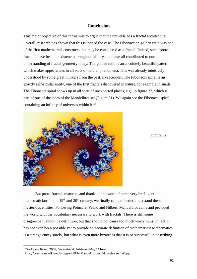
62

Conclusion

This major objective of this thesis was to argue that the universe has a fractal architecture.

Overall, research has shown that this is indeed the case. The Fibonaccian golden ratio was one

of the first mathematical constructs that may be considered as a fractal. Indeed, such ‘proto-

fractals’ have been in existence throughout history, and have all contributed to our

understanding of fractal geometry today. The golden ratio is an absolutely beautiful pattern

which makes appearances in all sorts of natural phenomena. This was already intuitively

understood by some great thinkers from the past, like Keppler. The Fibonacci spiral is an

exactly self-similar entity, one of the first fractals discovered in nature, for example in snails.

The Fibonacci spiral shows up in all sorts of unexpected places, e.g., in figure 32, which is

part of one of the sides of the Mandelbrot set (Figure 31). We again see the Fibonacci spiral,

containing an infinity of universes within it.26

But proto-fractals matured, and thanks to the work of some very intelligent

mathematicians in the 19th and 20th century, we finally came to better understand these

mysterious entities. Following Poincare, Peano and Hilbert, Mandelbrot came and provided

the world with the vocabulary necessary to work with fractals. There is still some

disagreement about the definition, but that should not cause too much worry in us, in fact, it

has not even been possible yet to provide an accurate definition of mathematics! Mathematics

is a strange entity surely, but what is even more bizarre is that it is so successful in describing

26 Wolfgang Beyer, 2006, December 4. Retrieved May 24 from: https://commons.wikimedia.org/wiki/File:Mandel_zoom_04_seehorse_tail.jpg

Figure 32

63

worldly phenomena, and it has permeated all sciences, from physics, to psychology and

sociology. Fractal geometry is the next big step in describing Nature, with the use of

mathematics.

We ventured in the world and saw that fractals appear almost everywhere. We have

seen examples of coastlines, trees, mountains, snowflakes, brains, organs, cells, proteins,

galaxies and nebulae. And we have only just begun, it is thrilling to think about where we

may find fractals next. Some researchers (including myself) have hinted at the possibility of

fractality in language, music or cognition (thoughts).

Studying galaxies as fractals is interesting in particular, because it makes us wonder

what the biggest scale is where describing galaxies with the fractal dimension D is possible.

Some scholars argue that there is no end, the fractality continues indefinitely. This would

probably mean that the universe itself is a fractal. Some, however, argue that there is a cutoff

point, and that the universe becomes smooth beyond a few hundred megaparsecs. This would

mean that the Cosmological Principle is true, and thus the universe is homogeneous and

isotropic at large enough scales.

The model we have of the universe follows the Cosmological Principle, namely the

Big Bang model. Much evidence (such as Hubble’s law, and the CMB) has pointed towards

the Big Bang being an accurate description of the birth and development of our universe.

However, the shape and the size of the universe remains elusive. There are various options

according to the calculations of Friedmann, the universe can be infinite or finite, and

spherical, hyperbolical or flat and Euclidean. Evidence has favored infinite and Euclidean, but

we cannot be completely sure yet. Until that time, we cannot say conclusively if the universe

as a whole is a fractal (or perhaps a multifractal system), or if it is just a simple shape which

contains a bunch of fractals. The only theories right now that can point at the universe being a

fractal are speculative, for example the theory of multiverses. But nonetheless, it has been

utterly clear that the universe contains many types of fractals, so it is legitimate to claim that

its architecture is fractal.

Lastly, the reader has been made aware that fractals are not entirely a very modern

concept. Great thinkers from the past have already had an intuition for objects that are self-

similar and infinitely complex. It is quite logical that when these individuals were thinking

about the universe (which also shows self-similarity and infinite complexity), that they saw

similarities between mathematical entities, the material world and the universe. If they had the

64

right tools and vocabulary, they most likely would have used fractals in their cosmological

models.

It is an absolute privilege to live in this day and age where our knowledge of the

universe has so vastly expanded. Human ingenuity is perplexing, which has allowed us to

look back 14 billion years in the past and make statements about that period with high

accuracy. And all of this knowledge has been won in the past centuries, whilst humans have

been around for tens of thousands of years. There is still an infinity of knowledge to be found,

and whilst this may seem like a hopeless project, I am certain that mankind will not lose hope,

and will keep pursuing this romantic endeavor of understanding the nature of the universe

fully.

It is my own suggestion that fractality will turn out to be a vital part of many aspects

of the universe. Fractality will be found in linguistics, music and cognition. I urge fellow

researchers to investigate these matters. The first place to look for fractality in linguistics is

with recursive acronyms. An acronym is an abbreviation that can be read as a word, e.g.,

NASA (which stands for “National Aeronautics and Space Administration”). A recursive

acronym is formed when one of the constituent words is the same as the whole! An example

from Hofstadter (1980) is GOD, where it stands for GOD Over Djinn (for the meaning of this,

I refer the reader to p. 113. The exact meaning is not really relevant here, what is more

important is its interesting expansion property). Clearly, this can be recursively iterated to

produce:

G(G(G(G(G(G(G(G(G(G … OD Over Djinn) OD Over Djinn) OD Over Djinn)

OD Over Djinn) OD Over Djinn) OD Over Djinn) OD Over Djinn) OD Over

Djinn) OD Over Djinn) OD Over Djinn).

where every G becomes expanded to contain “GOD Over Djinn”, which has to be performed

an infinite amount of times to reach the end. Accordingly, the “…” stands for the infinite gap

between the beginning and the end. This is similar to how the equation of the golden ratio can

be expanded. If we move the “1” term to the right in equation (1.9), we get

𝜑𝜑 = 1 + 1𝜑𝜑

. (6.1)

But we can replace the 𝜑𝜑 in 1𝜑𝜑

by 1 + 1𝜑𝜑

, since 𝜑𝜑 = 1 + 1𝜑𝜑

, which gives

65

𝜑𝜑 = 1 + 11+1

𝜑𝜑 . (6.2)

Cleary, we can repeat this an infinite amount of times, yielding

𝜑𝜑 = 1 + 11+ 1

1+ 11+ 1

1+ 11+1…

. (6.3)

The similarities here, between something linguistic, and the golden ratio which goes on to

produce infinitely varied fractals, is quite clear. I encourage other researchers to consider how

the fractal dimension might relate to recursive acronyms, or other facets of language that seem

to embody recursivity.

My last concluding remark and suggestion to the reader is to appreciate the infinite.

People in the past might have become uncomfortable with such a notion of infinity. For

example, Zeno’s paradox might have caused people to become distressed, and conclude that

the notion of movement is too absurd to even think about! But it turns out that infinity is

absolutely everywhere in our daily lives, we simply choose not to be aware of it. Being able to

deal with infinitesimals in the time of Newton and Leibniz has revolutionized calculus in

mathematics, and now infinitely recursive formulae has caused a revolution of geometry, and

hence fractal geometry was born. It is incomprehensible what type of beautiful patterns can be

made, by taking a simple formula and iterating it to infinity on the computer. It makes one

wonder, if the universe has not also been created in a similar way: with only a few simple

rules, which is iterated to infinity. Perhaps someday, we can learn to understand these simple

principles.

66

List of references

Abell, G. O. (1958). The distribution of rich clusters of galaxies. The Astrophysical Journal

Supplement Series, 3, 211.

Baryshev, Y., & Teerikorpi, P. (2002). Discovery of cosmic fractals. World Scientific.

Blanton, R. E., Levitt, J. G., Thompson, P. M., Narr, K. L., Capetillo-Cunliffe, L., Nobel, A.,

& Toga, A. W. (2001). Mapping cortical asymmetry and complexity patterns in

normal children. Psychiatry Research: Neuroimaging, 107(1), 29-43.

"Brief Answers to Cosmic Questions". www.cfa.harvard.edu. Archived from the original on

13 April 2016. Retrieved 16 March 2018.

Bullmore, E., Brammer, M., Harvey, I., Persaud, R., Murray, R., & Ron, M. (1994). Fractal

analysis of the boundary between white matter and cerebral cortex in magnetic

resonance images: a controlled study of schizophrenic and manic-depressive

patients. Psychological Medicine, 24(3), 771-781.

Combes, F. (2000). Astrophysical fractals: interstellar medium and galaxies. In The Chaotic

Universe (pp. 143-172).

Dickau, J. J. (2009). Fractal cosmology. Chaos, Solitons & Fractals, 41(4), 2103-2105.

Duffy, L. D., & Van Bibber, K. (2009). Axions as dark matter particles. New Journal of

Physics, 11(10), 105008.

Dunlap, R. A. (1997). The golden ratio and Fibonacci numbers. World Scientific.

Elert, G. (2003). The chaos hypertextbook: Mathematics in the age of the computer. Glenn

Elert.

Elmegreen, B. G., & Elmegreen, D. M. (2001). Fractal structure in galactic star fields. The

Astronomical Journal, 121(3), 1507.

Enright, M. B., & Leitner, D. M. (2005). Mass fractal dimension and the compactness of

proteins. Physical Review E, 71(1), 011912.

Falconer, K. (2004). Fractal geometry: mathematical foundations and applications. John

Wiley & Sons.

Feder, J. (2013). Fractals. Springer Science & Business Media.

67

Fitzpatrick, R. (2006). Euclid's Elements in Greek. Lulu. com.

Havlin, S., Buldyrev, S. V., Goldberger, A. L., Mantegna, R. N., Ossadnik, S. M., Peng, C.

K., & Stanley, H. E. (1995). Fractals in biology and medicine. Chaos, Solitons &

Fractals, 6, 171-201.

Herbst, E. (1995). Chemistry in the interstellar medium. Annual Review of Physical

Chemistry, 46(1), 27-54.

Hofstadter, D. H. (1980). Gödel, Escher, Bach: An Eternal Golden Braid;[a Metaphoric

Fugue on Minds and Machines in the Spirit of Lewis Carroll]. Penguin Books.

Howel, E. (2014. March 21). “What Is The Hubble Constant?” Space.com. Retrieved May 21,

2018 from: https://www.space.com/25179-hubble-constant.html

Hubble, E. (1926). No. 324. Extra-galactic nebulae. Contributions from the Mount Wilson

Observatory/Carnegie Institution of Washington, 324, 1-49.

Kedzia, A., Rybaczuk, M., & Andrzejak, R. (2002). Fractal dimensions of human brain cortex

vessels during the fetal period. Medical Science Monitor, 8(3), MT46-MT51.

Kraut, Richard. (2017). "Plato", The Stanford Encyclopedia of Philosophy. Retrieved from:

https://plato.stanford.edu/archives/fall2017/entries/plato/

Liu, J. Z., Zhang, L. D., & Yue, G. H. (2003). Fractal dimension in human cerebellum

measured by magnetic resonance imaging. Biophysical Journal, 85(6), 4041-4046.

Livio, M. (2008). The golden ratio: The story of phi, the world's most astonishing number.

Broadway Books.

Mandelbrot, B. (1983). The fractal geometry of nature (Vol. 173). New York: WH

Freeman.

Mandelbrot, B. (1967). How long is the coast of Britain? Statistical self-similarity and

fractional dimension. Science, 156(3775), 636-638.

Monnerot-Dumaine, A. (2009). The Fibonacci word fractal.

Nadler, S. (2008). A companion to early modern philosophy. John Wiley & Sons.

Overbye, Dennis (2017, February 20). "Cosmos Controversy: The Universe Is Expanding, but

How Fast?". New York Times. Retrieved 22 May 2018.

68

Redd, N.T. (2017). Milky Way Galaxy: Facts About Our Galactic Home. Retrieved from:

https://www.space.com/19915-milky-way-galaxy.html

Peitgen, H. O., Jürgens, H., & Saupe, D. (2006). Chaos and fractals: new frontiers of science.

Springer Science & Business Media.

Rohlf, M. (2016). "Immanuel Kant", The Stanford Encyclopedia of Philosophy. Retrieved

from: https://plato.stanford.edu/archives/spr2016/entries/kant/

Schadé, J. P. (1987). Atlas van het menselijk lichaam. De Tijdstroom.

Sernetz, M., Wübbeke, J., & Wlczek, P. (1992). Three-dimensional image analysis and fractal

characterization of kidney arterial vessels. Physica A: Statistical Mechanics and its

Applications, 191(1-4), 13-16.

Spinoza, B. (1883). Ethic: Demonstrated in Geometrical Order… . Trübner.

Wright, E. L. (2009, May 9). "What is the evidence for the Big Bang?". Frequently Asked

Questions in Cosmology. UCLA, Division of Astronomy and Astrophysics.

Retrieved May 21, 2018 from:

http://www.astro.ucla.edu/~wright/cosmology_faq.html#BBevidence