PLATFORM DEVELOPMENT AND PATH FOLLOWING CONTROLLER DESIGN

FOR FULL-SIZED VEHICLE AUTOMATION

by

Austin D. Costley

A thesis submitted in partial fulfillmentof the requirements for the degree

of

MASTER OF SCIENCE

in

Electrical Engineering

Approved:

Rajnikant Sharma, Ph.D. Don Cripps, Ph.D.Major Professor Committee Member

Xiaojun Qi, Ph.D. Mark R. McLellan, Ph.D.Committee Member Vice President for Research and

Dean of the School of Graduate Studies

UTAH STATE UNIVERSITYLogan, Utah

2017

ii

Copyright © Austin D. Costley 2017

All Rights Reserved

iii

ABSTRACT

Platform Development and Path Following Controller Design for Full-Sized Vehicle

Automation

by

Austin D. Costley, Master of Science

Utah State University, 2017

Major Professor: Rajnikant Sharma, Ph.D.Department: Electrical and Computer Engineering

The purpose of this thesis is to explore the challenges of reverse engineering the commu-

nication protocols of a stock 2013 Ford Focus EV, and build an open-source automation

platform to control the vehicle. The automated platform could be used to research modern

vehicle systems security, control system design and implementation, and automated sys-

tems design. This thesis will discuss the development of the automation platform and the

components used in the final design.

During the reverse engineering stages of this work, important security concerns were

identified in the Controller Area Network (CAN) architecture of the vehicle. The archi-

tecture allowed for arbitrary vehicle acceleration to be commanded through CAN message

injection. It was shown that the acceleration message could be sent from a tap point on the

CAN bus, or through the diagnostics (OBD-II) port. The vehicle would accept the injected

message, and the vehicle would accelerate without error. Another approach explored in this

work is to control the vehicle by emulating the output of the accelerator pedal, brake pedal,

and steering torque sensors. The latter approach was ultimately used to control the vehicle.

The controller design for the autonomous system was a successive loop closure method

where the low-level controllers would control vehicle speed and steering wheel angle, and the

iv

high-level controller would follow a path and provide commands for the low-level controllers.

Before controllers were designed, a model identification approach was used to obtain transfer

functions between the input signals and the vehicle.

A major barrier for researchers to perform automated vehicle research is the cost.

There are a variety of hardware and software systems available to aid in the development of

automation process, but they are often very expensive. This work is provided as an open-

source solution for the software and hardware design. The component selection process for

this project was heavily influenced by the cost of the component and the accessibility of

open-source software to interface with the component. The overall cost of the automation

platform was under $2,500, and the software has been made available to the public.

(70 pages)

v

PUBLIC ABSTRACT

Platform Development and Path Following Controller Design for Full-Sized Vehicle

Automation

Austin D. Costley

The purpose of this thesis is to discuss the design and development of a platform used

to automate a stock 2013 Ford Focus EV. The platform is low-cost and open-source to

encourage collaboration and provide a starting point for fellow researchers to advance the

work in the field of automated vehicle control. This thesis starts by discussing the process

of obtaining control of the vehicle by taking advantage of internal communication protocols.

The controller design process is detailed and a description of the components and software

used to control the vehicle is provided. The automated system is tested and the results of

fully autonomous driving are discussed.

vi

To my sweetheart, Jacqueline.

vii

ACKNOWLEDGMENTS

I express my sincere gratitude to Dr. Rajnikant Sharma for his mentorship, teaching,

and enthusiasm. His encouragement to pursue a Master’s Degree was instrumental in my

development as an engineer. I would also like to thank Dr. Don Cripps for his passion for

control systems engineering, which has been an inspiration to me and has helped determine

the direction I am taking my career. I would like to thank Dr. Xiaojun Qi for her excitement

and encouragement for this research. I would also like to acknowledge Dr. Ryan Gerdes

who provided excellent direction and mentorship. The success of this work was greatly

influenced by his contributions.

Many thanks to the EVAutomation Team at Utah State University who helped lay the

foundation for this work. In particular, thanks to my research partner, Chase Kunz, who

was instrumental in making this dream possible.

Last, but certainly not least, I would like to express my sincere appreciation to my

wife, Jacqueline, who has been an unfailing source of inspiration and support. I would also

like to thank my parents for their constant encouragement.

Austin D. Costley

viii

CONTENTS

Page

ABSTRACT . . . . . . . . . . . . . . . . . . . . . . . . . . . . . . . . . . . . . . . . . . . . . . . . . . . . . . iii

PUBLIC ABSTRACT . . . . . . . . . . . . . . . . . . . . . . . . . . . . . . . . . . . . . . . . . . . . . . . v

ACKNOWLEDGMENTS . . . . . . . . . . . . . . . . . . . . . . . . . . . . . . . . . . . . . . . . . . . . vii

LIST OF TABLES . . . . . . . . . . . . . . . . . . . . . . . . . . . . . . . . . . . . . . . . . . . . . . . . . x

LIST OF FIGURES . . . . . . . . . . . . . . . . . . . . . . . . . . . . . . . . . . . . . . . . . . . . . . . . xi

ACRONYMS . . . . . . . . . . . . . . . . . . . . . . . . . . . . . . . . . . . . . . . . . . . . . . . . . . . . . xiii

CHAPTER

1 INTRODUCTION . . . . . . . . . . . . . . . . . . . . . . . . . . . . . . . . . . . . . . . . . . . . . . . 11.1 Literature Review . . . . . . . . . . . . . . . . . . . . . . . . . . . . . . . . 11.2 Contributions . . . . . . . . . . . . . . . . . . . . . . . . . . . . . . . . . . . 4

2 EMULATE COMMUNICATIONS AND ENABLE REMOTE CONTROL . . . . . . 52.1 Vehicle Architecture and Approach . . . . . . . . . . . . . . . . . . . . . . . 52.2 CAN Message Injection . . . . . . . . . . . . . . . . . . . . . . . . . . . . . 82.3 Sensor Emulation . . . . . . . . . . . . . . . . . . . . . . . . . . . . . . . . . 122.4 CAN Message Injection Through OBD-II . . . . . . . . . . . . . . . . . . . 15

3 MODEL IDENTIFICATION AND LOW-LEVEL CONTROLLER DESIGN . . . . . 193.1 Longitudinal Model . . . . . . . . . . . . . . . . . . . . . . . . . . . . . . . . 193.2 Lateral Model . . . . . . . . . . . . . . . . . . . . . . . . . . . . . . . . . . . 243.3 PI Controller Design . . . . . . . . . . . . . . . . . . . . . . . . . . . . . . . 30

4 HIGH-LEVEL CONTROLLER DESIGN . . . . . . . . . . . . . . . . . . . . . . . . . . . . . . 334.1 Differential Flatness . . . . . . . . . . . . . . . . . . . . . . . . . . . . . . . 334.2 Control Architecture . . . . . . . . . . . . . . . . . . . . . . . . . . . . . . . 35

5 AUTOMATION PLATFORM OVERVIEW . . . . . . . . . . . . . . . . . . . . . . . . . . . . 375.1 Interfacing Architecture . . . . . . . . . . . . . . . . . . . . . . . . . . . . . 38

5.1.1 Microcontroller and Associated Hardware . . . . . . . . . . . . . . . 385.1.2 Other Interface Devices . . . . . . . . . . . . . . . . . . . . . . . . . 40

5.2 Sensing Architecture . . . . . . . . . . . . . . . . . . . . . . . . . . . . . . . 415.3 Computational Architecture . . . . . . . . . . . . . . . . . . . . . . . . . . . 43

5.3.1 Microcontroller Software . . . . . . . . . . . . . . . . . . . . . . . . . 445.3.2 ROS Architecture . . . . . . . . . . . . . . . . . . . . . . . . . . . . 44

ix

6 EXPERIMENTAL RESULTS . . . . . . . . . . . . . . . . . . . . . . . . . . . . . . . . . . . . . . . 476.1 Low Level Controller . . . . . . . . . . . . . . . . . . . . . . . . . . . . . . . 476.2 Path and Velocity Errors of Autonomous Driving . . . . . . . . . . . . . . . 48

7 CONCLUSION . . . . . . . . . . . . . . . . . . . . . . . . . . . . . . . . . . . . . . . . . . . . . . . . . 527.1 Conclusion . . . . . . . . . . . . . . . . . . . . . . . . . . . . . . . . . . . . 52

REFERENCES . . . . . . . . . . . . . . . . . . . . . . . . . . . . . . . . . . . . . . . . . . . . . . . . . . . 54

x

LIST OF TABLES

Table Page

2.1 Sensor and Module Connections for Control Signals . . . . . . . . . . . . . . 8

3.1 Parameters for Low-Level Controllers . . . . . . . . . . . . . . . . . . . . . . 32

5.1 Microcontroller Peripherals Table . . . . . . . . . . . . . . . . . . . . . . . . 44

7.1 Itemized Cost Breakdown of Automation Platform . . . . . . . . . . . . . . 52

xi

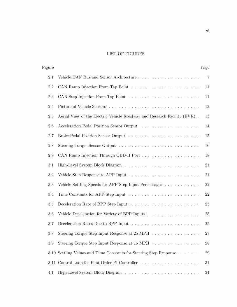
LIST OF FIGURES

Figure Page

2.1 Vehicle CAN Bus and Sensor Architecture . . . . . . . . . . . . . . . . . . . 7

2.2 CAN Ramp Injection From Tap Point . . . . . . . . . . . . . . . . . . . . . 11

2.3 CAN Step Injection From Tap Point . . . . . . . . . . . . . . . . . . . . . . 11

2.4 Picture of Vehicle Sensors . . . . . . . . . . . . . . . . . . . . . . . . . . . . 13

2.5 Aerial View of the Electric Vehicle Roadway and Research Facility (EVR) . 13

2.6 Acceleration Pedal Position Sensor Output . . . . . . . . . . . . . . . . . . 14

2.7 Brake Pedal Position Sensor Output . . . . . . . . . . . . . . . . . . . . . . 15

2.8 Steering Torque Sensor Output . . . . . . . . . . . . . . . . . . . . . . . . . 16

2.9 CAN Ramp Injection Through OBD-II Port . . . . . . . . . . . . . . . . . . 18

3.1 High-Level System Block Diagram . . . . . . . . . . . . . . . . . . . . . . . 21

3.2 Vehicle Step Response to APP Input . . . . . . . . . . . . . . . . . . . . . . 21

3.3 Vehicle Settling Speeds for APP Step Input Percentages . . . . . . . . . . . 22

3.4 Time Constants for APP Step Input . . . . . . . . . . . . . . . . . . . . . . 22

3.5 Deceleration Rate of BPP Step Input . . . . . . . . . . . . . . . . . . . . . . 23

3.6 Vehicle Deceleration for Variety of BPP Inputs . . . . . . . . . . . . . . . . 25

3.7 Deceleration Rates Due to BPP Input . . . . . . . . . . . . . . . . . . . . . 25

3.8 Steering Torque Step Input Response at 25 MPH . . . . . . . . . . . . . . . 27

3.9 Steering Torque Step Input Response at 15 MPH . . . . . . . . . . . . . . . 28

3.10 Settling Values and Time Constants for Steering Step Response . . . . . . . 29

3.11 Control Loop for First Order PI Controller . . . . . . . . . . . . . . . . . . 31

4.1 High-Level System Block Diagram . . . . . . . . . . . . . . . . . . . . . . . 34

xii

5.1 Platform Diagram . . . . . . . . . . . . . . . . . . . . . . . . . . . . . . . . 39

5.2 Printed Circuit Board and Microcontroller . . . . . . . . . . . . . . . . . . . 40

5.3 Piksi RTK-GPS, CANalyzer, and PCAN Device . . . . . . . . . . . . . . . 41

5.4 Trunk Setup of Automation Platform in 2013 Ford Focus EV . . . . . . . . 42

5.5 Serial Message Structure . . . . . . . . . . . . . . . . . . . . . . . . . . . . . 45

6.1 Steering Angle Step Response without Deadband Compensation . . . . . . 49

6.2 Steering Angle Step Response with Deadband Compensation . . . . . . . . 50

6.3 Trajectory and Path of Autonomous Vehicle . . . . . . . . . . . . . . . . . . 50

6.4 Desired and Actual Velocity of Autonomous Vehicle . . . . . . . . . . . . . 51

6.5 Velocity and Path Error of Autonomous Vehicle . . . . . . . . . . . . . . . . 51

xiii

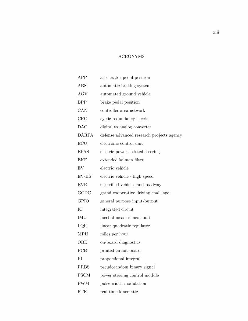
ACRONYMS

APP accelerator pedal position

ABS automatic braking system

AGV automated ground vehicle

BPP brake pedal position

CAN controller area network

CRC cyclic redundancy check

DAC digital to analog converter

DARPA defense advanced research projects agency

ECU electronic control unit

EPAS electric power assisted steering

EKF extended kalman filter

EV electric vehicle

EV-HS electric vehicle - high speed

EVR electrified vehicles and roadway

GCDC grand cooperative driving challenge

GPIO general purpose input/output

IC integrated circuit

IMU inertial measurement unit

LQR linear quadratic regulator

MPH miles per hour

OBD on-board diagnostics

PCB printed circuit board

PI proportional integral

PRBS pseudorandom binary signal

PSCM power steering control module

PWM pulse width modulation

RTK real time kinematic

xiv

ROS robot operating system

TCM transmission control module

UART universal asynchronous receiver/transmitter

UAV unmanned aerial vehicle

UPS uninterpretable power supply

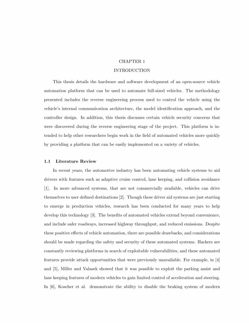
CHAPTER 1

INTRODUCTION

This thesis details the hardware and software development of an open-source vehicle

automation platform that can be used to automate full-sized vehicles. The methodology

presented includes the reverse engineering process used to control the vehicle using the

vehicle’s internal communication architecture, the model identification approach, and the

controller design. In addition, this thesis discusses certain vehicle security concerns that

were discovered during the reverse engineering stage of the project. This platform is in-

tended to help other researchers begin work in the field of automated vehicles more quickly

by providing a platform that can be easily implemented on a variety of vehicles.

1.1 Literature Review

In recent years, the automotive industry has been automating vehicle systems to aid

drivers with features such as adaptive cruise control, lane keeping, and collision avoidance

[1]. In more advanced systems, that are not commercially available, vehicles can drive

themselves to user defined destinations [2]. Though these driver aid systems are just starting

to emerge in production vehicles, research has been conducted for many years to help

develop this technology [3]. The benefits of automated vehicles extend beyond convenience,

and include safer roadways, increased highway throughput, and reduced emissions. Despite

these positive effects of vehicle automation, there are possible drawbacks, and considerations

should be made regarding the safety and security of these automated systems. Hackers are

constantly reviewing platforms in search of exploitable vulnerabilities, and these automated

features provide attack opportunities that were previously unavailable. For example, in [4]

and [5], Miller and Valasek showed that it was possible to exploit the parking assist and

lane keeping features of modern vehicles to gain limited control of acceleration and steering.

In [6], Koscher et al. demonstrate the ability to disable the braking system of modern

2

vehicles.

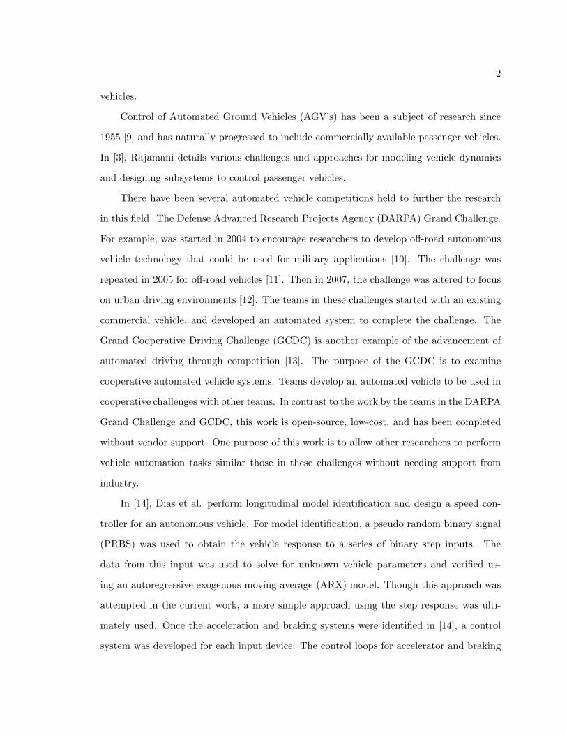
Control of Automated Ground Vehicles (AGV’s) has been a subject of research since

1955 [9] and has naturally progressed to include commercially available passenger vehicles.

In [3], Rajamani details various challenges and approaches for modeling vehicle dynamics

and designing subsystems to control passenger vehicles.

There have been several automated vehicle competitions held to further the research

in this field. The Defense Advanced Research Projects Agency (DARPA) Grand Challenge.

For example, was started in 2004 to encourage researchers to develop off-road autonomous

vehicle technology that could be used for military applications [10]. The challenge was

repeated in 2005 for off-road vehicles [11]. Then in 2007, the challenge was altered to focus

on urban driving environments [12]. The teams in these challenges started with an existing

commercial vehicle, and developed an automated system to complete the challenge. The

Grand Cooperative Driving Challenge (GCDC) is another example of the advancement of

automated driving through competition [13]. The purpose of the GCDC is to examine

cooperative automated vehicle systems. Teams develop an automated vehicle to be used in

cooperative challenges with other teams. In contrast to the work by the teams in the DARPA

Grand Challenge and GCDC, this work is open-source, low-cost, and has been completed

without vendor support. One purpose of this work is to allow other researchers to perform

vehicle automation tasks similar those in these challenges without needing support from

industry.

In [14], Dias et al. perform longitudinal model identification and design a speed con-

troller for an autonomous vehicle. For model identification, a pseudo random binary signal

(PRBS) was used to obtain the vehicle response to a series of binary step inputs. The

data from this input was used to solve for unknown vehicle parameters and verified us-

ing an autoregressive exogenous moving average (ARX) model. Though this approach was

attempted in the current work, a more simple approach using the step response was ulti-

mately used. Once the acceleration and braking systems were identified in [14], a control

system was developed for each input device. The control loops for accelerator and braking

3

were connected by switching logic to determine whether the accelerator or brakes should be

used. A similar two-loop control system with a switching logic component was used for the

longitudinal controller in the current work. However, the current work is open-source and

uses the Robot Operating System (ROS) [15].

Ferrin et al., implemented a state feedback controller on a differentially flat Unmanned

Aerial Vehicle (UAV) system in [16]. The high level controller structure and differentially

flat techniques were modified for ground vehicles and implemented in this work.

Koscher et al. and Checkoway et al. in [17] and [6] showed that an attacker can

gain access to Electronic Control Units (ECU’s) and circumvent vehicle control and safety

systems. They also demonstrated that the attacker could gain access to the Controller

Area Network (CAN) bus remotely, and perform similar attacks. Their results included

the ability to have the car ignore a brake pedal press by the driver, a complete vehicle

shut down, and complete control of the visual display. The attacks however, did not allow

for arbitrary control of acceleration, braking or steering; which are all required for vehicle

autonomy.

Miller and Valasek built on the work from Koscher et. al. and Checkoway et. al.

in [4] and [5], which detail attacks on vehicle systems in a 2010 Ford Escape, 2010 Toyota

Prius, and a 2014 Jeep Cherokee. They developed an extensive platform for attacking

ECU’s and exploiting driver assist systems. However, the attacks had limited scope for

vehicle control. For example, an attack on the parking assist module was conducted on

the 2010 Ford Escape, whereby, vehicle steering could be controlled when the vehicle was

traveling at under 5 mph. However, this attack would not work if the vehicle was moving

faster. They also demonstrated the ability to cause vehicle acceleration under very specific

conditions. In contrast, this work demonstrates the ability to cause arbitrary acceleration

under any condition. In addition, using the approach presented here, the acceleration can

be controlled from the OBD-II port, any bus tap point, or by gaining access to an ECU.

The current work also demonstrates the security concern that a vehicle could be examined

and reverse engineered in a short amount of time, as it took a small team of students just

4

under a year to develop the automated system for a commercial vehicle.

1.2 Contributions

The contributions of this thesis are as follows:

• The process of reverse engineering the communication protocols of the CAN modules

and sensors in the 2013 Ford Focus Electric is detailed in Chapter 2. Two approaches

for obtaining remote control of the vehicle are examined: CAN message injection and

sensor emulation.

• Security concerns involving the communication architecture of the vehicle are pre-

sented. Arbitrary vehicle acceleration is demonstrated by injecting CAN messages

from a tap point on the bus, and through the on-board diagnostics port (OBD-II).

• A simple model identification approach using the step response for the available in-

puts is given in Chapter 3. The design for the speed and steering controllers is also

presented.

• Chapter 4 discusses the high-level path follower controller design using differential

flatness and state-feedback.

• Chapter 5 gives an overview of the platform architecture and details the hardware

and software components of the automation platform.

The experimental results for the controllers and resulting automated vehicle are given in

Chapter 6. The findings are summarized and the thesis is concluded in Chapter 7.

5

CHAPTER 2

EMULATE COMMUNICATIONS AND ENABLE REMOTE CONTROL

This chapter details the efforts of a group of undergraduate researchers at Utah State

University in reverse engineering the communication signals of a 2013 Ford Focus EV.

Methods for identifying sensor output signals and CAN messages are discussed and results

from the vehicle of interest are presented. An approach injecting CAN messages to cause ve-

hicle acceleration is given, and a sensor emulation approach is shown to control acceleration,

braking, and steering.

A team of undergraduate students in the Electrical and Mechanical Engineering pro-

grams at Utah State University (including the author of this work) was assembled to explore

the 2013 Ford Focus Electric and reverse engineer the communication protocols. The work

from this team is detailed in the first part of this chapter. The reverse engineering project

lasted from November 2015 to May 2016. The next stage of the project was led by the

author of this work, and his research partner, Chase Kunz. It is important to note the

collaboration effort with Chase, and identify his contributions. In particular, Chase was

instrumental in developing the CAN injection architecture and in discovering the message

required to accelerate the vehicle through CAN message insertion (Chapter 2.2). He also

helped with the model identification and low-level controller design (Chapter 3).

2.1 Vehicle Architecture and Approach

Modern vehicles use a Controller Area Network (CAN) bus system for module-to-

module communication [18]. Electronic Control Units (ECU’s) are the CAN modules that

connect to the bus that send and receive information. A CAN module receives data from

sensors, processes the data, and generates the appropriate CAN message to be broadcast

on the bus using an analog-to-digital operation.

6

The research team for the current work used the 2013 Ford Focus Electric Wiring

Guide [19] and the Auto Repair Reference Center Research Database from EBSCOhost [20]

to understand signal path and critical connections. The wiring guide provided diagrams for

most of the wires in the vehicle, and included diagrams and pin-outs for the wiring con-

nections. The Auto Repair Reference Center was particularly useful for reverse engineering

the CAN protocols. It contains the CAN messages generated and received by each module,

diagrams of the four CAN buses in the vehicle, and the module layout on each bus. The

CAN message information was an incomplete list of general messages sent between CAN

modules. For example, the list would indicate that a message about the acceleration pedal

position is sent from one module to another, but it would not indicate the structure of the

message, the arbitration ID, or a conversion to useful units.

Using these resources, the team identified sensors and modules that could be used

for vehicle control. Table 2.1 summarizes these findings. In addition, the team took a

hands-on approach to vehicle exploration, and verified the location and connections of these

components.

The examination of this architecture led to the identification of the two possible con-

troller insertion strategies, as shown in Fig. 2.1. First, the CAN lines between the control

module and the CAN bus could be cut, and a controller could be inserted to intercept

and change messages being sent from the target control module. Second, the analog signal

wires from the target sensor could be cut, and the controller could be inserted between the

sensor and the control module. In either strategy, the controller would insert spurious data

into the system to control the vehicle. The details and results of these two approaches are

discussed in the following subsections.

In order to successfully implement the first controller insertion strategy and take ad-

vantage of the information on the vehicle CAN bus, the Vector CANalyzer [21] system was

used for the initial CAN message identification process. This system provides an excellent

visual tool for watching CAN messages in real time. The tool displays a table of CAN

messages with rows organized by arbitration ID. The first column of the table indicates the

7

ABS TCM

PCMPSCM APPSTS

BPP

Controller Insertion Type 1 - CAN Message Injection

Controller Insertion Type 2 - Sensor Emulation

ABS Automatic Braking System Module

TCM Transmission Control Module

PCM Powertrain Control Module

APP Accelerator Pedal Position Sensor

CAN Bus Wires

Analog Signal Wire

STS Steering Torque Sensor

CAN Bus Module

Vehicle Sensors

BusTermination

BusTermination

ActuatesBraking

ActuatesSteering

ActuatesAcceleration

Sends throttlemessageto TCM

Fig. 2.1: Vehicle CAN bus and sensor architecture. Controller insertion type 1 filters CANmessages and replaces data with the message to be injected, and is represented by a filledblack square. Controller insertion type 2 emulates sensor output signals, and are representedby filled black circles. The TCM controls the main drive motor of the electric vehicle, andtherefore actuates acceleration. The PSCM actuates the power steering motor. The ABSmodule actuates the hydraulic braking system.

8

Table 2.1: Sensor and Module Connections for Control SignalsSensor CAN Module CAN Message CAN Arbitration ID

Accelerator Pedal Position Sensor Powertrain Control Module (PCM) Accelerator Pedal Position 0x204Brake Pedal Position Sensor Automatic Braking System (ABS) Brake Pedal Position 0x7DSteering Torque Sensor Power Steering Control Module (PSCM) Steering Torque UnknownSteering Wheel Angle Sensor Steering Angle Sensor Module (SASM) Steering Wheel Angle 0x10

time since the last message with a given arbitration ID was received. The second column

lists the arbitration ID, and the third column shows the value for each byte of the CAN

message. If a byte is changed when a new message is received, the byte is displayed in

bold. Over time, the byte fades to a light gray if that value stays the same. This was

useful in identifying messages such as the accelerator pedal position, brake pedal position,

steering wheel angle, and vehicle speed. The CANalyzer system is a great resource, but it

is expensive and closed-source. Cheaper alternatives such as the Peak Systems PCAN [22]

device can be used that have an open platform for development. An open-source solution

for monitoring CAN traffic with the PCAN device is provided with the open-source software

accompanying this work. Further discussion on the use of the PCAN device can be found

in Chapter 5.1. Another alternative is to use a microcontroller with a CAN bus interface

module to monitor and report CAN traffic [23].

Using the resources in the previous paragraphs, it was determined that CAN messages

have two main functions: status and control. A status message reports the status of a vehicle

component or condition, but does not control that component or condition. For example,

a module will receive input from the wheel speed sensors and send the information on the

CAN bus. Changing the data in this message will not result in a change of vehicle speed.

A control message, however, is sent by a module to control a component or condition of the

vehicle. For example, the movement of the wing mirrors is controlled by a CAN signal, and

when this message is changed, the mirrors will move in response.

2.2 CAN Message Injection

A platform for injecting CAN messages was developed using the TI TM4C129XL mi-

crocontroller evaluation kit [23] and TI CAN transceivers [24]. The platform would connect

to the CAN bus using the first controller insertion point, located between the target module

9

and the bus. The microcontroller was programmed to record and playback CAN traffic.

More specifically, the microcontroller would receive the output from the control module

and store it in memory. Upon user request, the output from the control module could be

injected on the CAN bus. This platform was used to determine which messages, organized

by arbitration ID, were generated by the target control module. Using information from

the Auto Repair Center Research Database, it was determined that the Powertrain Control

Module (PCM) sent a CAN message to the Transmission Control Module (TCM) regarding

the accelerator pedal position. In addition, the PCM was the only control module that re-

ceived the sensor signal from the accelerator pedal. For these reasons, the PCM was chosen

as the target module for vehicle acceleration.

The connector diagrams in the Wiring Guide were used to determine the CAN bus

connections to the PCM. These wires were cut and routed to the CAN injection platform.

The CAN messages output from the PCM were recorded and passed through to the CAN

bus for an accelerator pedal press. The recorded data was then played back on the bus and

the vehicle accelerated as expected. Additional code was added to the playback function to

selectively playback messages based on the message arbitration ID. This was used to search

the recorded data set and isolate the acceleration control message. The messages were

separated into two groups based on their arbitration ID, and each group was played back

to the vehicle separately. The group that resulted in vehicle acceleration was separated

again into two smaller groups. The process was repeated until one message arbitration

ID was left. The acceleration control message was determined to be the message with

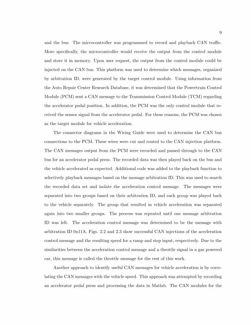
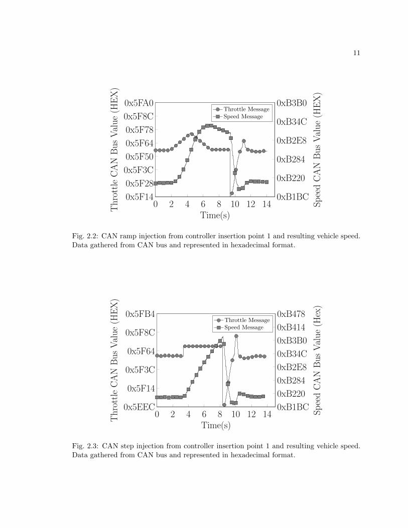
arbitration ID 0x11A. Figs. 2.2 and 2.3 show successful CAN injections of the acceleration

control message and the resulting speed for a ramp and step input, respectively. Due to the

similarities between the acceleration control message and a throttle signal in a gas powered

car, this message is called the throttle message for the rest of this work.

Another approach to identify useful CAN messages for vehicle acceleration is by corre-

lating the CAN messages with the vehicle speed. This approach was attempted by recording

an accelerator pedal press and processing the data in Matlab. The CAN modules for the

10

2013 Ford Focus EV broadcast messages at prescribed frequencies; as opposed to broad-

casting in response to another signal. The speed message for the vehicle is broadcast at

100 Hz, which is the highest frequency messages are broadcast for this vehicle. Correlation

was performed on messages of the same frequency, and the speed data was downsampled to

perform correlation with messages at lower frequencies. The correlation returned a value

between -1 and 1 for each byte of every message to indicate how closely correlated that byte

was to the speed message. If the byte did not change during the recording, the correlation

returned NAN. On the EV-HS CAN bus, there are 102 different messages; each message

contains 8 bytes. The bytes were sorted based on the absolute value of the correlation value

to identify the highest positively or negatively correlated bytes. The bytes that had a NAN

value were rejected, and the final number of bytes being ranked was 341. The highest cor-

related byte of 0x11A was byte 4, which had a correlation value of 0.2359 and was ranked

57 out of 341. The low correlation value and rank indicates that the throttle message would

not have been identified using this strategy. In contrast, using the approach described in

the previous paragraph, the throttle message was identified and was used to control vehicle

acceleration.

The investigation of the braking system concluded that a CAN bus message about

pedal position would not actuate the hydraulic braking system. The pedal signal is sent

directly to the Automatic Braking System (ABS) CAN module, which is the only CAN

module on the vehicle that is connected to the hydraulic brake lines. From this, it was

concluded that braking could not be fully controlled through the CAN bus.

The 2013 Ford Focus EV has an option to include park assist [25]. Though our specific

vehicle did not include this option, it was determined that the Electric Power Assisted

Steering (EPAS) system had the same part number and motor as the EPAS system in a

vehicle with the park assist feature. This meant that the power steering motor would be

powerful enough to turn the wheel at low speeds, and by extension, any speed. The Power

Steering Control Module (PSCM) receives inputs from the CAN bus and the steering torque

sensor located at the base of the steering column. The torque sensor uses a torsion bar to

11

0x5F14

0x5F28

0x5F3C

0x5F50

0x5F64

0x5F78

0x5F8C

0x5FA0ThrottleCANBusValue(H

EX)

0 2 4 6 8 10 12 140xB1BC

0xB220

0xB284

0xB2E8

0xB34C

0xB3B0

Time(s)

SpeedCANBusValue(H

EX)

Throttle MessageSpeed Message

Fig. 2.2: CAN ramp injection from controller insertion point 1 and resulting vehicle speed.Data gathered from CAN bus and represented in hexadecimal format.

0x5EEC

0x5F14

0x5F3C

0x5F64

0x5F8C

0x5FB4

ThrottleCANBusValue(H

EX)

0 2 4 6 8 10 12 140xB1BC

0xB220

0xB284

0xB2E8

0xB34C

0xB3B0

0xB414

0xB478

Time(s)

SpeedCANBusValue(H

ex)

Throttle MessageSpeed Message

Fig. 2.3: CAN step injection from controller insertion point 1 and resulting vehicle speed.Data gathered from CAN bus and represented in hexadecimal format.

12

determine the amount of torque being applied by the driver, which is used by the PSCM

to determine how much assist the power steering motor should provide. Simply, for a given

torque input, less assistance would be provided by the EPAS system at higher speeds.

Similar to the brake system, the input of interest is sent from a sensor to the module that

performs the desired action. This led to the conclusion that the control of steering would

have to be controlled through torque sensor input, and not through the CAN bus. In

addition, the work by Miller and Valasek [5] [4] identifies the shortcomings of exploiting

the park assist feature; the park assist feature will cease to control the vehicle if the speed

threshold is exceeded.

2.3 Sensor Emulation

The CAN bus injection method was unable to control braking and steering, so the

sensor emulation method was explored. The accelerator pedal position sensor was analyzed

to control vehicle acceleration, the brake pedal position sensor was analyzed to control the

braking system, and the steering torque sensor was analyzed to control the vehicle steering.

Fig. 2.4 shows these sensors, and the following paragraphs discuss the analysis.

The accelerator pedal position (APP) sensor is located at the top of the accelerator

pedal. There are six wires connected to the APP sensor, including two 5 V power wires with

corresponding ground wires, and two signal wires. The sensor power pins were connected to

a voltage source, and the signal wires were connected to an oscilloscope. It was determined

that the sensor outputs two DC voltages similar to the output of potentiometers. Fig. 2.6

shows the voltage levels of the two output signals in response to a pedal press. The third

signal on the graph is a multiplier that relates the two signals. It is seen that V1 ≈ 2V2.

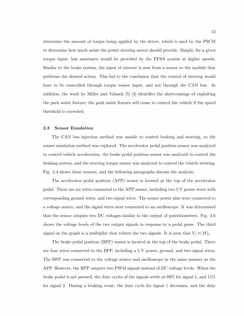
The brake pedal position (BPP) sensor is located at the top of the brake pedal. There

are four wires connected to the BPP, including a 5 V power, ground, and two signal wires.

The BPP was connected to the voltage source and oscilloscope in the same manner as the

APP. However, the BPP outputs two PWM signals instead of DC voltage levels. When the

brake pedal is not pressed, the duty cycles of the signals settle at 89% for signal 1, and 11%

for signal 2. During a braking event, the duty cycle for signal 1 decreases, and the duty

13

Fig. 2.4: The physical sensors emulated for vehicle control. Top: Steering rack for 2013Ford Focus EV, the steering torque sensor is located at the base of the steering columnand measures torque from driver. Bottom Left: The APP sensor located at the top of theaccelerator pedal. Bottom Right: The BPP sensor that is usually mounted behind the brakepedal assembly, which measures the brake pedal press.

Fig. 2.5: Aerial view of the Electric Vehicle Roadway and Research Facility (EVR) at UtahState University.

14

0 5 10 15 20 25 300

1

2

3

4

Time (s)

Volts

(v)

Signal 1 (V1)Signal 2 (V2)Multiplier (V1/V2)

Fig. 2.6: Acceleration pedal position sensor output. Two analog voltage signals related byV1 = 2V2.

cycle for signal 2 increases at the same rate. Fig. 2.7 shows the two PWM signals for the

BPP. The frequency of signal 1 is 533 Hz and the frequency of signal 2 is 482 Hz.

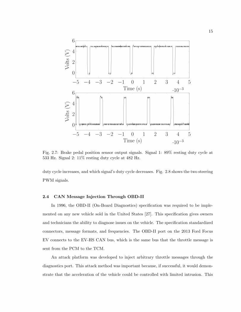
The steering torque sensor is located at the base of the steering column. The sensor

connects to the Power Steering Control Module (PSCM) on the CAN bus, which determines

the amount of power steering assist to provide. The assist is provided by an electric motor

connected to the steering rack. In the sensor, a torsion bar is used to connect two parts

of the steering shaft, where the rotational displacement can be measured to determine the

torque input by the driver [26]. Similar to the BPP, there are 4 wires connected to the

steering torque sensor, including 5 V power, ground, and two signal wires. The steering

torque sensor was connected to the voltage source and oscilloscope, and it was determined

that the sensor outputs two PWM signals on the signal wires, where both signals settle

at 50% duty cycle when no torque is applied on the steering wheel. Both signals have a

frequency of 2.15 kHz. Similar to the brake PWM signals, the duty cycles always add to

100%, and the direction that the steering wheel is being turned determines which signal’s

15

−5 −4 −3 −2 −1 0 1 2 3 4 5

·10−3

0

2

4

6

Time (s)

Volts

(V)

−5 −4 −3 −2 −1 0 1 2 3 4 5

·10−3

0

2

4

6

Time (s)

Volts

(V)

Fig. 2.7: Brake pedal position sensor output signals. Signal 1: 89% resting duty cycle at533 Hz. Signal 2: 11% resting duty cycle at 482 Hz.

duty cycle increases, and which signal’s duty cycle decreases. Fig. 2.8 shows the two steering

PWM signals.

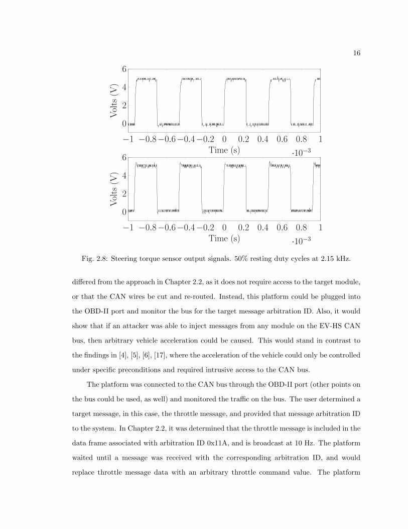
2.4 CAN Message Injection Through OBD-II

In 1996, the OBD-II (On-Board Diagnostics) specification was required to be imple-

mented on any new vehicle sold in the United States [27]. This specification gives owners

and technicians the ability to diagnose issues on the vehicle. The specification standardized

connectors, message formats, and frequencies. The OBD-II port on the 2013 Ford Focus

EV connects to the EV-HS CAN bus, which is the same bus that the throttle message is

sent from the PCM to the TCM.

An attack platform was developed to inject arbitrary throttle messages through the

diagnostics port. This attack method was important because, if successful, it would demon-

strate that the acceleration of the vehicle could be controlled with limited intrusion. This

16

−1 −0.8−0.6−0.4−0.2 0 0.2 0.4 0.6 0.8 1

·10−3

0

2

4

6

Time (s)

Volts

(V)

−1 −0.8−0.6−0.4−0.2 0 0.2 0.4 0.6 0.8 1

·10−3

0

2

4

6

Time (s)

Volts

(V)

Fig. 2.8: Steering torque sensor output signals. 50% resting duty cycles at 2.15 kHz.

differed from the approach in Chapter 2.2, as it does not require access to the target module,

or that the CAN wires be cut and re-routed. Instead, this platform could be plugged into

the OBD-II port and monitor the bus for the target message arbitration ID. Also, it would

show that if an attacker was able to inject messages from any module on the EV-HS CAN

bus, then arbitrary vehicle acceleration could be caused. This would stand in contrast to

the findings in [4], [5], [6], [17], where the acceleration of the vehicle could only be controlled

under specific preconditions and required intrusive access to the CAN bus.

The platform was connected to the CAN bus through the OBD-II port (other points on

the bus could be used, as well) and monitored the traffic on the bus. The user determined a

target message, in this case, the throttle message, and provided that message arbitration ID

to the system. In Chapter 2.2, it was determined that the throttle message is included in the

data frame associated with arbitration ID 0x11A, and is broadcast at 10 Hz. The platform

waited until a message was received with the corresponding arbitration ID, and would

replace throttle message data with an arbitrary throttle command value. The platform

17

was designed to only alter the parts of the message that relate to the throttle control.

The inserted message would be sent 250 µs after the actual message, leaving 9.75 ms for

the inserted message to be received and processed by the TCM. This allowed the inserted

message to dominate the period and cause the vehicle to accelerate. Fig. 2.9 shows the

successful ramp injection through the OBD-II port and the resulting vehicle speed. Thus

confirming the hypothesis that vehicle acceleration can be caused by injecting CAN messages

through the OBD-II port, and therefore, could be caused at any other point on the bus.

These results demonstrate a CAN bus security concern. If an attacker were able to

access the CAN bus, physically, or by compromising another ECU, they would be able

to effect the acceleration of the vehicle without causing any errors. Remote access to the

vehicle, but not necessarily the requisite CAN bus, could be affected by compromising the

Telematic Control Unit (TCU) or a wireless Tire Pressure Monitoring Sensor (TPMS).

The TPMS sends a signal to the Body Control Module (BCM), which in turn transmits

a message on the medium speed CAN bus (MS-CAN), while the TCU is connected to the

I-CAN bus (it is unlikely, however, that compromising a sensor would allow for injection of

arbitrary CAN messages onto the I-CAN or MS-CAN bus). These buses are connected to

the EV-HS bus through a gateway module; transmitting a message from one bus to another,

which would be required for either the TCU or TPMS to impersonate the PCM by passing

APP messages, was not explored in this work. Regardless of the access approach, the driver

is able to stop the unwanted acceleration by pressing the brake pedal. However, other works

indicate that it is possible to make the vehicle ignore braking requests [5] [4] [17] [6]. This

was not investigated as part of this work. Another security concern is that of a malicious

technician. Since technicians will often access the OBD-II port when a vehicle is being

serviced, it would be quite simple for them to leave an OBD-II injection platform connected

to the OBD-II port. The acceleration control could be initiated remotely, or by a timer,

causing the vehicle to accelerate at a dangerous time.

We present two remediation strategies that could be employed to help protect against

this vulnerability. First, a simple change in the acceleration system architecture, such

18

0 2 4 6 8 10 12 140x5F00

0x5F28

0x5F50

0x5F78

0x5FA0

Time (s)

ThrottleCANBusValue(H

EX)

0xB1BC

0xB220

0xB284

0xB2E8

0xB34C

0xB3B0

SpeedCANBusValue(H

ex)

Car Throttle MessageInjected Throttle MessageSpeed Message

Fig. 2.9: CAN ramp injection through OBD-II port with resulting vehicle speed. Injectedthrottle message was sent on bus immediately following car throttle message. Values readfrom CAN bus and displayed in hexadecimal format.

that the APP sensor connects directly to the TCM, which is the actuating module. This

would remove the need of a throttle message to be sent from the PCM to the TCM and

effectively remove the attack surface. The second approach is through device fingerprinting

for both the digital and analog signals [28] [29]. This would allow the receiving module to

authenticate the transmitting module, and prevent this type of attack.

19

CHAPTER 3

MODEL IDENTIFICATION AND LOW-LEVEL CONTROLLER DESIGN

This chapter details the model identification techniques used in this work. A simple first

order step response technique was used to design low-level controllers to control vehicle speed

and steering wheel angle. The design process of the low-level controllers is also discussed.

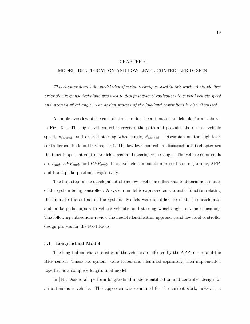
A simple overview of the control structure for the automated vehicle platform is shown

in Fig. 3.1. The high-level controller receives the path and provides the desired vehicle

speed, vdesired, and desired steering wheel angle, θdesired. Discussion on the high-level

controller can be found in Chapter 4. The low-level controllers discussed in this chapter are

the inner loops that control vehicle speed and steering wheel angle. The vehicle commands

are τcmd, APPcmd, and BPPcmd. These vehicle commands represent steering torque, APP,

and brake pedal position, respectively.

The first step in the development of the low level controllers was to determine a model

of the system being controlled. A system model is expressed as a transfer function relating

the input to the output of the system. Models were identified to relate the accelerator

and brake pedal inputs to vehicle velocity, and steering wheel angle to vehicle heading.

The following subsections review the model identification approach, and low level controller

design process for the Ford Focus.

3.1 Longitudinal Model

The longitudinal characteristics of the vehicle are affected by the APP sensor, and the

BPP sensor. These two systems were tested and identified separately, then implemented

together as a complete longitudinal model.

In [14], Dias et al. perform longitudinal model identification and controller design for

an autonomous vehicle. This approach was examined for the current work, however, a

20

more straightforward classical controls technique using step responses was ultimately used.

Once the acceleration and braking systems were identified, a control system was developed

for each input device. The control loops for accelerator and braking were connected by

switching logic to determine whether the accelerator or brakes should be used. A similar

two loop control system with a switching logic component was used for the longitudinal

controller in the current work. However, this work is an open-source project that uses the

Robot Operating System (ROS) [15].

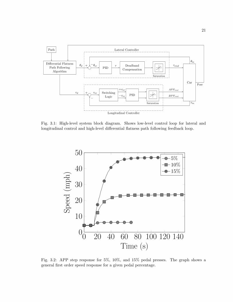
For the APP sensor system identification, the vehicle was placed on a dynamometer [30]

and step inputs were initiated on the APP sensor from 4% to 15%, at increments of 1%.

Fig. 3.2 shows the step responses for some accelerator pedal inputs. It was observed that

for a given APP percentage, the vehicle would eventually settle at a specific speed. The

relationship between APP and speed can be described by a first order transfer function.

The general equation for a first order transfer function, G(s), can be represented by

G(s) =K

τs+ 1. (3.1)

Where K is the constant or equation that relates APP to vehicle speed, and τ is the system

time constant. The equation for K was derived from a linear fit of the a scatter plot of max

speeds from the step input, as shown in Fig. 3.3, and given by

f(x) = 3.65x− 9.7. (3.2)

Where f(x) is the vehicle speed, and x is the APP percentage. The test track (shown in Fig.

2.5) where the vehicle was operating is an oval track with sharp corners on the north and

south side. The sharp corners and the short straightaways limit the vehicle operating speeds

to between 15 and 25 mph for the initial automation. The τ value that best represented the

vehicle response between 15 and 25 mph was chosen as the time constant for accelerator

pedal input in the longitudinal model. Fig. 3.4 shows the time constants for varying APP

percentages. The time constant for the accelerator pedal input was chosen to be 7 seconds,

21

Differential FlatnessPath Following

AlgorithmPID

DeadbandCompensation

Saturation

SwitchingLogic

PID

Saturation

Car

τcmd+θd θer τ

θm−

vm

−

+vd ver+ver

−ver

APPcmd

BPPcmd

Pose

Longitudinal Controller

Lateral ControllerPath

Fig. 3.1: High-level system block diagram. Shows low-level control loop for lateral andlongitudinal control and high-level differential flatness path following feedback loop.

0 20 40 60 80 100 120 1400

10

20

30

40

50

Time (s)

Speed(m

ph)

5%

10%

15%

Fig. 3.2: APP step response for 5%, 10%, and 15% pedal presses. The graph shows ageneral first order speed response for a given pedal percentage.

22

4 6 8 10 12 14 160

10

20

30

40

50

APP %

Speed(m

ph)

Fig. 3.3: Vehicle settling speeds for given APP step input percentages.

4 6 8 10 12 14 160

5

10

15

APP %

Tim

e(s)

Fig. 3.4: Time constants for given APP step input percentages.

23

67 68 69 70 71

−0.3

−0.2

−0.1

0

Time (s)

DecelerationRate(m

/s2)

Fig. 3.5: Deceleration rate for BPP step input of 15%. The figure shows a first orderrelationship between BPP percentage and deceleration rate.

as this best represented the system response for the nominal operating conditions.

For BPP system identification, the vehicle was driven in a large, flat, asphalt area at

speeds ranging from 5 to 25 mph, at 5 mph increments. The vehicle was accelerated to

the desired speed by a driver. Once the vehicle obtained the desired speed, an input to

the braking system was initiated through the ROS system discussed in Chapter 5. Step

inputs were initiated, ranging from 5% to 50% of BPP percentage, at increments of 5%

for each speed value. The speed data seemed to show a consistent rate of change for

a given BPP percentage. To confirm this, the speed data was smoothed using a 5 point

moving average. The derivative of the smoothed data was taken by calculating the difference

between successive data points, and dividing by the elapsed time between data points. Fig.

3.5 shows the vehicle deceleration due to a braking event. It was observed that the settling

value for the deceleration rate was consistent for a given BPP percentage and varying speeds,

which concluded that the longitudinal model was independent of current vehicle speed.

This speed independence can be seen in Fig. 3.6, where each line shows the deceleration

24

rate for a given BPP percentage. At low BPP values, the lines converge, meaning that

deceleration is unaffected by very small brake pedal percentages. However, at higher brake

pedal percentages, the lines show distinct deceleration rates regardless of the vehicle speed.

To show the relationship between BPP percentage and deceleration, an average was taken

for each BPP value across each of the speeds. The result of this operation is shown in Fig.

3.7.

Similar to the APP model, the relationship between BPP and deceleration could be

described by a first order transfer function. After analyzing the deceleration curves at dif-

ferent BPP percentages and for different speeds, the system time constant, τ , was calculated

to be 0.3 seconds. The equation that relates BPP to deceleration was determined by finding

a curve fit algorithm for the curve in Fig. 3.7. This would result in an equation that would

provide a BPP percentage for a desired deceleration rate. The equation for K is given by

f(x) = −0.0018x2 + 0.029x− 0.3768, (3.3)

where f(x) is the deceleration, and x is the BPP percentage. This equation is used to

describe K from the general first order transfer function equation.

3.2 Lateral Model

The lateral model of the vehicle was determined by step response analysis. The model

relates an input from the steering torque sensor to changes in the steering wheel angle. As

discussed in Chapter 2.3, the torque sensor measures the torque applied by the driver, and

sends that information to the PSCM. The PSCM activates the power assist motor that

connects to the steering rack, and moves the wheels. The steering wheel angle is measured

by a sensor in the steering wheel and output on the CAN bus.

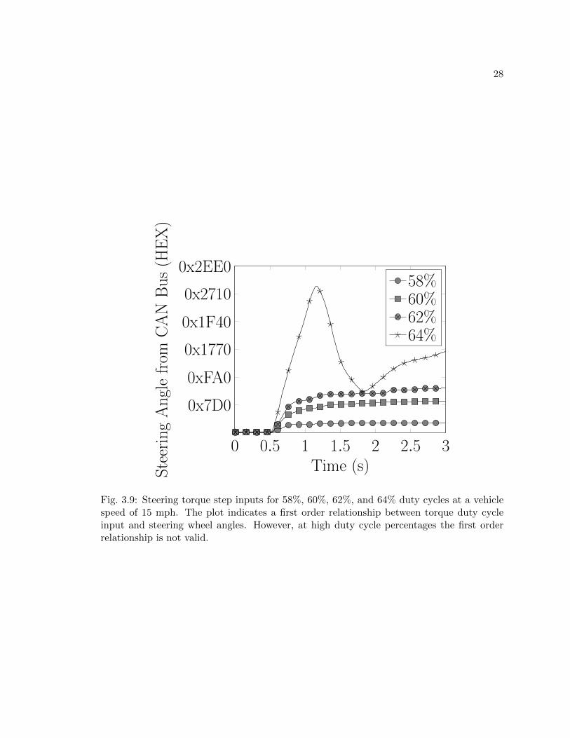
Step inputs were initiated on the steering torque duty cycle signal, ranging from 50%

to 63%, at 1% increments. Tests were performed at a large, flat, asphalt area with vehicle

speeds ranging from 5 mph to 25 mph. Fig. 3.8 shows the results of the step input tests

performed at 25 mph. It was observed that a general first order transfer function could

25

6 8 10 12 14 16 18 20 22 24

−3

−2

−1

0

Speed (mph)

Deceleration(m

/s2) 15%

25%

30%

35%

40%

45%

50%

Fig. 3.6: Vehicle deceleration for BPP percentages at a variety of speeds. The values arethe average of the deceleration rates settling point in response to a BPP step input. Thelines for BPP percentages do not cross, and therefore, indicate speed independence for thebrake model.

10 20 30 40 50

−3

−2

−1

0

BPP (%)

Deceleration(m

/s2)

Fig. 3.7: Average deceleration settling rates due to BPP step input percentages.

26

be used to describe the relationship between steering torque duty cycle and steering wheel

angle. However, at lower speeds and higher torque values, this observation is not valid. Fig.

3.9 shows the step response of the steering system at 15 mph. At the higher torque values,

the steering wheel angles do not settle to a consistent steering wheel angle. It was also

observed that the settling angles for a given steering torque duty cycle are not consistent

for varying speeds. Therefore, the lateral model identification is speed dependent and

would require a speed dependent limit on the steering torque duty cycle. Providing these

characteristics, the system can still be modeled as first order transfer function for a given

speed.

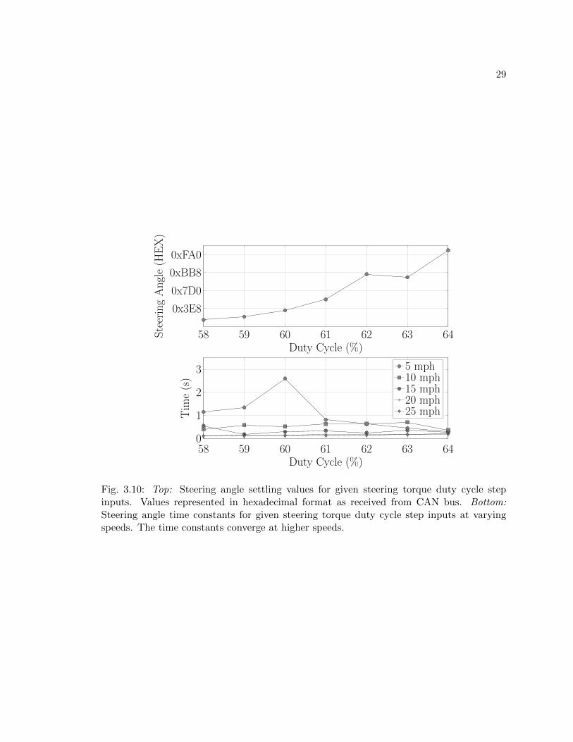
The steering data was analyzed in order to determine the gain equation, K, and the

time constant, τ . Time constants were calculated for each step input response, and for each

speed. Fig. 3.10 Bottom shows the time constants for given steering torque duty cycles.

Each of the lines indicates the speed at which the test was performed. It can be seen that at

low speeds and low duty cycles, the time constants are not consistent, but at higher speeds,

the inconsistencies lessen. A time constant, τ , of 0.2 seconds was chosen to optimize for

typical vehicle operation.

Since the lateral system was found to be speed dependent, the gain equation K must

also be speed dependent. The step input tests were performed at 5 mph increments so a gain

equation K would be found for each speed value. These gain equations relate steering torque

duty cycle to steering wheel angle. Fig. 3.10 shows the settling angles for varying steering

torque duty cycles when the vehicle was traveling at 25 mph. A curve fit approximation was

completed for this data set, and a solution was determined by solving the given equation.

For this data set, the given equation for K is

f(x) = 59.4x2 − 6802.7x+ 195084.5, (3.4)

where f(x) is the steering wheel angle, and x is the steering torque duty cycle.

Figs. 3.8 and 3.9 show the step response of the vehicle due to steering torque input

signals. The graphs do not include step input values below 58% because the step responses

27

0 0.5 1 1.5 2 2.5 3

0x1F4

0x3E8

0x5DC

0x7D0

0x9C4

0xBB8

0xDAC

Time (s)SteeringAnglefrom

CANBus(H

EX)

58%60%62%64%

Fig. 3.8: Steering torque step response for 58%, 60%, 62%, and 64% duty cycles at a vehiclespeed of 25 mph. The plot indicates a first order relationship between torque duty cycleinput and steering wheel angle.

28

0 0.5 1 1.5 2 2.5 3

0x7D0

0xFA0

0x1770

0x1F40

0x2710

0x2EE0

Time (s)SteeringAnglefrom

CANBus(H

EX)

58%60%62%64%

Fig. 3.9: Steering torque step inputs for 58%, 60%, 62%, and 64% duty cycles at a vehiclespeed of 15 mph. The plot indicates a first order relationship between torque duty cycleinput and steering wheel angles. However, at high duty cycle percentages the first orderrelationship is not valid.

29

58 59 60 61 62 63 64

0x3E8

0x7D0

0xBB8

0xFA0

Duty Cycle (%)

SteeringAngle(H

EX)

58 59 60 61 62 63 640

1

2

3

Duty Cycle (%)

Tim

e(s)

5 mph10 mph15 mph20 mph25 mph

Fig. 3.10: Top: Steering angle settling values for given steering torque duty cycle stepinputs. Values represented in hexadecimal format as received from CAN bus. Bottom:Steering angle time constants for given steering torque duty cycle step inputs at varyingspeeds. The time constants converge at higher speeds.

30

at such values had little effect on the steering wheel angle. This exposed a deadband in the

response from the steering torque sensor input to the steering wheel angle. A deadband

compensation algorithm was implemented to mitigate the effects of this non-linearity. As

shown in Fig. 3.1, the deadband compensation code was executed just before the signal

was sent to the vehicle. If the torque input value was greater than 50%, then

τcmd = Bmax +τ − 50

τmax − 50(τmax −Bmax) (3.5)

was used to compensate for the deadband. If the torque input value was less than 50%,

then

τcmd = Bmin +50 − τ

50 − τmin(τmin −Bmin) (3.6)

was used to compensate for the deadband. Where τcmd is the torque command sent to

the vehicle, τ is the value received from the PI controller, Bmax is the upper limit of the

deadband, Bmin is the lower limit of the deadband, τmax is the maximum allowed value for

the steering torque signal, and τmin is the minimum allowed steering torque signal. For the

deadband on the 2013 Ford Focus EV, the upper and lower limits were 55% and 45%, and

the maximum and minimum values for the torque signal were 64% and 37%, respectively.

3.3 PI Controller Design

Low-level control loops were designed to control vehicle speed and steering wheel angle.

The desired speed and desired steering wheel angle would be input to the low-level control

loops from a user or high-level controller. The low-level longitudinal controller interfaced

with the accelerator and brake pedals to effect vehicle speed. A separate loop was designed

for each vehicle input, and switching logic was used to choose whether the acceleration or

brake loop would be used. The low-level lateral controller would receive the desired steering

wheel angle and determine the appropriate input to the steering torque sensor to achieve

the desired angle.

A Proportional Integral (PI) Feedback Controller was implemented for longitudinal

31

and lateral control. Fig. 3.11 shows a basic PI Feedback Controller for a first order system.

The transfer function block represents the vehicle and contains the system model. The

1K block effectively cancels out the gain equation K, and helps relate the speed error to a

vehicle input. For example, in the longitudinal controller, the K equation receives the APP

as an input, and outputs speed. Therefore, the input to the transfer function block must be

an APP value. However, the control loop is calculating a speed error, so the output of the

PI block is a speed value. The 1K block translates the speed value into appropriate APP

value.

Since the K and 1K can be combined to equal 1, they can be ignored in the loop

equation. The open loop transfer function of this system is then given by

GOL(s) =1

(τs+ 1). (3.7)

Closing the feedback loop and adding the PI controller gives

GCL(s) =

kpτ

(s+ ki

kp

)s2 +

(1τ + kp

τ

)s+ ki

τ

. (3.8)

The system is stable if the real part of the closed-loop poles are negative. Solving for the

closed loop poles and zero yields

s =− (kp+ 1) ±

√(kp + 1)2 − 4kiτ

2τ, (3.9)

PI 1K

Kτs+1

in out

−

Controller Vehicle Model

Fig. 3.11: General control loop for a first order PI controller.

32

and

s = − kikp, (3.10)

respectively. From these equations, it can be determined that if kp and ki are positive, the

system will be stable.

The second order transfer function obtained through closing the loop can be written,

in a general form, as

ω2n

s2 + 2ζωns+ ω2n

. (3.11)

Where ζ is the damping coefficient and ωn is the natural frequency. The damping coefficient

determines whether the system will be under damped, over damped, or critically damped,

and the natural frequency helps to determine the time constant for the system. The time

constant, τ , is given by the equation τ = 1ζωn

. Values were chosen for the damping coefficient

and the time constant to define the system behavior. From these values, one can determine

the appropriate kp and ki for the system. The equations for kp and ki are given by

kp = τ

(2ζωn −

1

τ

), (3.12)

and

ki = τω2n, (3.13)

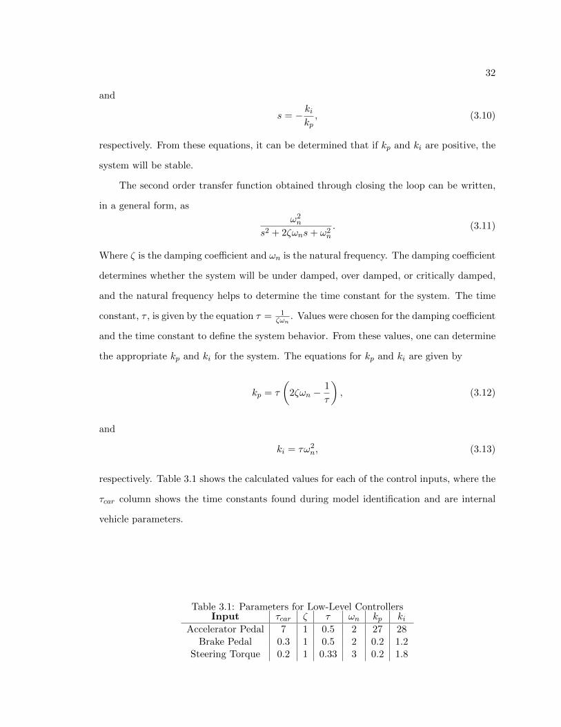
respectively. Table 3.1 shows the calculated values for each of the control inputs, where the

τcar column shows the time constants found during model identification and are internal

vehicle parameters.

Table 3.1: Parameters for Low-Level ControllersInput τcar ζ τ ωn kp ki

Accelerator Pedal 7 1 0.5 2 27 28Brake Pedal 0.3 1 0.5 2 0.2 1.2

Steering Torque 0.2 1 0.33 3 0.2 1.8

33

CHAPTER 4

HIGH-LEVEL CONTROLLER DESIGN

This chapter discusses the high-level path following controller design. The system is

shown to be differentially flat and a state feedback approach with a feed forward term is

presented.

The high-level controller was designed to take a desired trajectory or path, and provide

appropriate inputs for the low-level controllers. There are a number of high-level control

strategies for manned and unmanned vehicle control [31] [32] [33]. The control strategy

should be determined by the system characteristics and the system objectives. This platform

was to be used on a ground vehicle to track a desired trajectory and was determined to

be differentially flat [34] for the chosen states. A differentially flat system is one in which

the output is a function of the system states, the input, and the derivatives of the input,

and both the states and the input are functions of the output and the derivatives of the

output. Therefore, a simple high level controller using the properties of a differentially flat

system, and state feedback control were chosen [35]. An example control system design for

a differently flat Unmanned Aerial Vehicle (UAV) system was demonstrated in [16]. The

following paragraphs discuss differential flatness, and the high-level controller architecture

shown in Fig. 4.1.

4.1 Differential Flatness

A system is said to be differentially flat if there exists an output vector y in the form

of

y = h(x, u, u, u, ...., u(r)

), (4.1)

34

SystemDifferential Flatness

ut = [vnt; vet]xt = [pnt; pet]

Trajectorypnt, pet, vnt, vet

k

+ut u y

+ y = x

x

−kx

−xt

Fig. 4.1: High-level system block diagram. Details the high-level control loop, and the pathfollowing algorithm. The system block contains the low-level control loops, and the vehicle.

such that,

x = φ(y, y, y, ...., y(r)

),

u = α(y, y, y, ...., y(r)

),

(4.2)

where h, φ, and α are smooth functions. The output of the differentially flat system can,

therefore, be defined by a function of the system states, the control input, u, and the

derivatives of u. The state vector and control input vector can each be described by a

function of the flat output, y, and its derivatives.

The state vector for this system was chosen to be

x =

pnpe

, (4.3)

35

where pn is the vehicle position in the north direction and pe is the vehicle position in the

east direction. The system input, u, is given by

u =

vnve

, (4.4)

where vn is the velocity in the north direction and ve is the velocity in the east direction.

The system output, y, is given by

y =

pnpe

. (4.5)

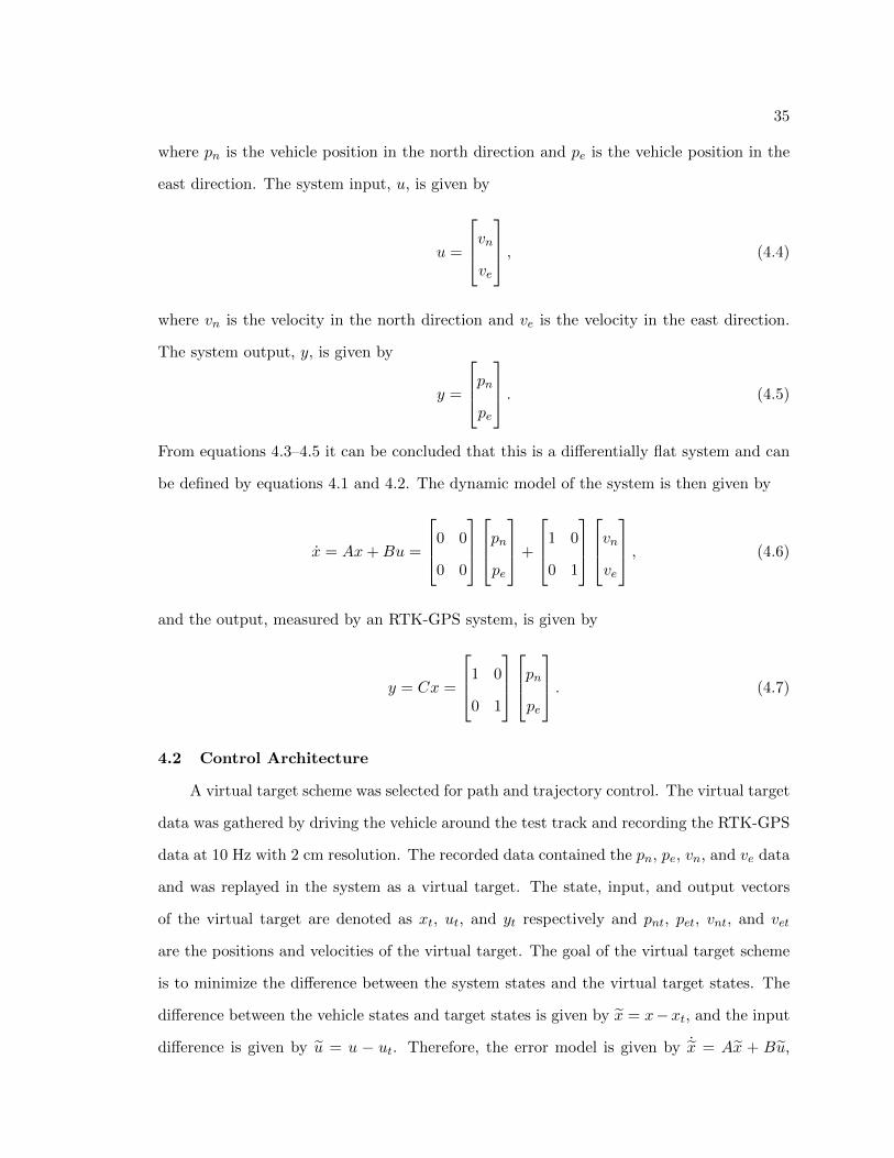
From equations 4.3–4.5 it can be concluded that this is a differentially flat system and can

be defined by equations 4.1 and 4.2. The dynamic model of the system is then given by

x = Ax+Bu =

0 0

0 0

pnpe

+

1 0

0 1

vnve

, (4.6)

and the output, measured by an RTK-GPS system, is given by

y = Cx =

1 0

0 1

pnpe

. (4.7)

4.2 Control Architecture

A virtual target scheme was selected for path and trajectory control. The virtual target

data was gathered by driving the vehicle around the test track and recording the RTK-GPS

data at 10 Hz with 2 cm resolution. The recorded data contained the pn, pe, vn, and ve data

and was replayed in the system as a virtual target. The state, input, and output vectors

of the virtual target are denoted as xt, ut, and yt respectively and pnt, pet, vnt, and vet

are the positions and velocities of the virtual target. The goal of the virtual target scheme

is to minimize the difference between the system states and the virtual target states. The

difference between the vehicle states and target states is given by x = x−xt, and the input

difference is given by u = u − ut. Therefore, the error model is given by ˙x = Ax + Bu,

36

where u is the commanded velocity vector. Solving for u, and using a state feedback control

strategy, where u = −kx gives u = ut − kx.

The Linear Quadratic Regulator (LQR) method was used to find the optimal gain

value for k. The entries in the system input vector, u, are notated by, u1 and u2, and are

used to obtain desired velocity by vd =√u21 + u22, and desired heading by ψd = tan−1

(u1u2

).

Through calculation and experimentation a relationship was determined between the desired

heading, ψd, and the desired steering wheel angle, θd. Such that, θd = kdψd. The desired

steering wheel angle and the desired velocity are sent to the low-level controllers discussed

in Chapter 3.

37

CHAPTER 5

AUTOMATION PLATFORM OVERVIEW

This chapter details the design and component selection for vehicle automation plat-

form. The hardware and software components are detailed and a link to the software repos-

itory is provided.

A versatile and robust platform is required to enable full-sized autonomous vehicle

research. The platform was designed to enable vehicle automation for both the CAN injec-

tion and the sensor emulation approaches discussed in Chapter 2.1. For the CAN injection

approach, the platform was able to monitor the CAN bus and inject the desired packets,

whereas for the sensor emulation approach, the platform required access to the output lines

of the sensors to be emulated. In order to proceed to autonomy, the platform required the

ability to sense the environment, determine vehicle location, communicate with the vehicle,

and monitor the CAN bus. A computer running Ubuntu and the Robot Operating System

(ROS) was used to communicate between the platform architectures. The computer was

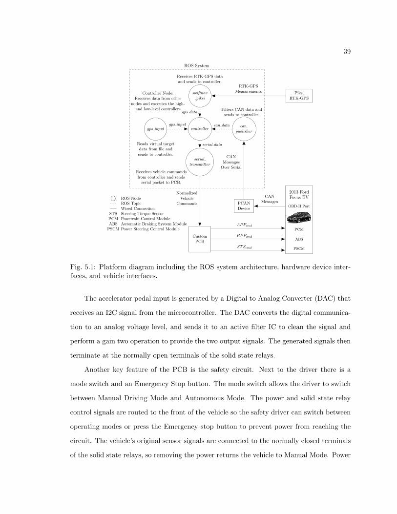
connected to a microcontroller to allow communication with the vehicle. Fig. 5.1 shows

a diagram of the autonomous system, including the ROS software architecture, hardware

connections to devices, and the vehicle interfacing hardware.

A ROS-based platform was chosen for ease of use, modularity, and sensor interfac-

ing packages. ROS is an open source framework that encourages collaboration between

researchers. People can contribute to the ROS effort by creating software packages that

interface with common sensors and provide tools for development. For example, an open-

source software package for ROS was provided by Swift Navigation to interface with the

Piksi RTK-GPS units [36], which helped expedite development time for this project. The

ROS architecture components used in this project are packages, nodes, and topics. A ROS

package is a collection of executable files used to complete a task. Generally packages are

38

used to compartmentalize similar parts of a project. ROS nodes are the executable files in

a ROS package that can be written in C/C++ or Python. A ROS topic is a way to transfer

data between nodes. Any node can publish data to a topic, and any node can subscribe to

that topic to receive the data. In this sense, the ROS topic acts as a bus to transfer data.

The following subsections detail the Interfacing Architecture, Sensing Architecture, and

the Computational Architecture of the automation platform.

5.1 Interfacing Architecture

Interfacing devices are critical to the success of vehicle automation as they provide

a way to send commands to the vehicle, and monitor the vehicle for feedback. A PCB

(shown in Fig. 5.2) was designed to provide a connection between the microcontroller and

the vehicle. The following subsections discuss the microcontroller and associated hardware,

and the other interfacing devices used for this platform.

5.1.1 Microcontroller and Associated Hardware

The TI TM4C129XL evaluation kit was the chosen microcontroller platform because

it offered multiple CAN bus interfaces allowing for a combination of CAN injection and

sensor emulation from the same board [23]. The microcontroller receives input from the

computer through a UART module. After performing the appropriate computations, PWM

signals are generated and appropriate DC voltage levels are determined for vehicle input.

The control signals pass through a variety of circuit components to prepare the signals

for vehicle injection. The signals are terminated at solid state relays that select either the

original vehicle signal, or the generated signal to be sent to the vehicle. The user determines

which signal is sent based on a mode switch input to the microcontroller.

The sensor emulation approach requires four PWM signals to be generated by the

microcontroller. The signals are passed through a level shifter to shift the amplitudes from

3.3 V to 5 V, and then sent through operational amplifiers in a voltage follower configuration

to help drive the signals. The PWM signals are then terminated at the normally opened

terminals of solid state relays.

39

ROS NodeROS TopicWired Connection

STS Steering Torque SensorPCM Powetrain Control ModuleABS Automatic Braking System Module

PSCM Power Steering Control Module

gps input controllercan

publisher

swiftnavpiksi

serialtransmitter

Reads virtual targetdata from file andsends to controller.

Filters CAN data andsends to controller.

Receives RTK-GPS dataand sends to controller.

Receives vehicle commandsfrom controller and sends

serial packet to PCB.

Controller Node:Receives data from other

nodes and executes the high-and low-level controllers.

PiksiRTK-GPS

PCANDevice

CustomPCB

2013 FordFocus EV

gps data

gps input can data

serial data

RTK-GPSMeasurements

CANMessages

Over Serial

NormalizedVehicle

Commands

CANMessages

APPcmd

BPPcmd

STScmd

ROS System

OBD-II Port

PCM

ABS

PSCM

Fig. 5.1: Platform diagram including the ROS system architecture, hardware device inter-faces, and vehicle interfaces.

The accelerator pedal input is generated by a Digital to Analog Converter (DAC) that

receives an I2C signal from the microcontroller. The DAC converts the digital communica-

tion to an analog voltage level, and sends it to an active filter IC to clean the signal and

perform a gain two operation to provide the two output signals. The generated signals then

terminate at the normally open terminals of the solid state relays.

Another key feature of the PCB is the safety circuit. Next to the driver there is a

mode switch and an Emergency Stop button. The mode switch allows the driver to switch

between Manual Driving Mode and Autonomous Mode. The power and solid state relay

control signals are routed to the front of the vehicle so the safety driver can switch between

operating modes or press the Emergency stop button to prevent power from reaching the

circuit. The vehicle’s original sensor signals are connected to the normally closed terminals

of the solid state relays, so removing the power returns the vehicle to Manual Mode. Power

40

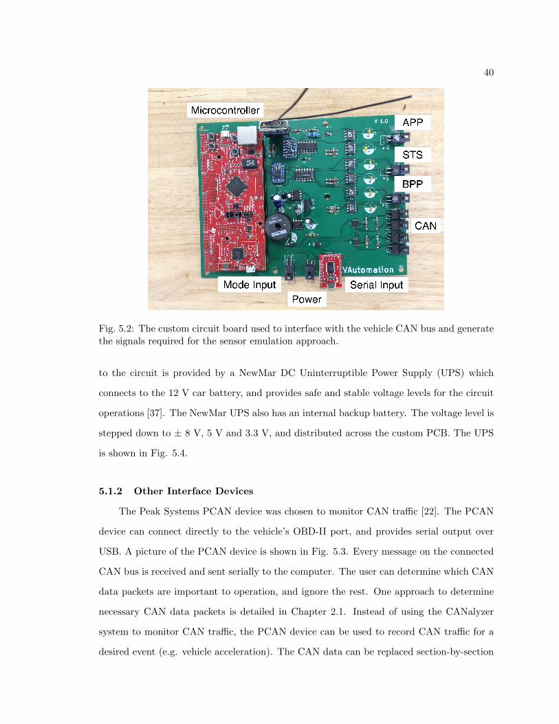
Fig. 5.2: The custom circuit board used to interface with the vehicle CAN bus and generatethe signals required for the sensor emulation approach.

to the circuit is provided by a NewMar DC Uninterruptible Power Supply (UPS) which

connects to the 12 V car battery, and provides safe and stable voltage levels for the circuit

operations [37]. The NewMar UPS also has an internal backup battery. The voltage level is

stepped down to ± 8 V, 5 V and 3.3 V, and distributed across the custom PCB. The UPS

is shown in Fig. 5.4.

5.1.2 Other Interface Devices

The Peak Systems PCAN device was chosen to monitor CAN traffic [22]. The PCAN

device can connect directly to the vehicle’s OBD-II port, and provides serial output over

USB. A picture of the PCAN device is shown in Fig. 5.3. Every message on the connected

CAN bus is received and sent serially to the computer. The user can determine which CAN

data packets are important to operation, and ignore the rest. One approach to determine

necessary CAN data packets is detailed in Chapter 2.1. Instead of using the CANalyzer

system to monitor CAN traffic, the PCAN device can be used to record CAN traffic for a

desired event (e.g. vehicle acceleration). The CAN data can be replaced section-by-section

41

Fig. 5.3: Left: The Piksi RTK-GPS unit with GPS antenna, radio antenna for communica-tion, and the Piksi module. Center: Vector CANalyzer system, used for reverse engineeringCAN messages. Right: The PCAN device used to interface with the vehicle CAN bus forhigh-level control feedback.

until a message, or set of messages, is isolated. Additional information on the use of the

PCAN device for system feedback is given in Chapter 5.3.2.

A USB-to-serial device was used between the microcontroller and computer to enable

communication. The control system determines the appropriate inputs to the vehicle and

sends the commands to the microcontroller. The device receives the signal from the USB

port and sends it to a UART module on the microcontroller. More information about the

microcontroller and control system is given in Chapter 5.3.

The TI SN65HVD230 CAN Transceiver Breakout Board [38] [24] was used to connect

the microcontroller to the CAN bus. This board provided a direct connection with the

vehicle CAN bus that can be used for monitoring and injection.

5.2 Sensing Architecture

The Swiftnav Piksi RTK-GPS unit [39] [40] was chosen to provide position and velocity

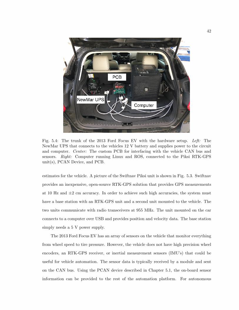
42

Fig. 5.4: The trunk of the 2013 Ford Focus EV with the hardware setup. Left: TheNewMar UPS that connects to the vehicles 12 V battery and supplies power to the circuitand computer. Center: The custom PCB for interfacing with the vehicle CAN bus andsensors. Right: Computer running Linux and ROS, connected to the Piksi RTK-GPSunit(s), PCAN Device, and PCB.

estimates for the vehicle. A picture of the Swiftnav Piksi unit is shown in Fig. 5.3. Swiftnav

provides an inexpensive, open-source RTK-GPS solution that provides GPS measurements

at 10 Hz and ±2 cm accuracy. In order to achieve such high accuracies, the system must

have a base station with an RTK-GPS unit and a second unit mounted to the vehicle. The

two units communicate with radio transceivers at 955 MHz. The unit mounted on the car

connects to a computer over USB and provides position and velocity data. The base station

simply needs a 5 V power supply.

The 2013 Ford Focus EV has an array of sensors on the vehicle that monitor everything

from wheel speed to tire pressure. However, the vehicle does not have high precision wheel

encoders, an RTK-GPS receiver, or inertial measurement sensors (IMU’s) that could be

useful for vehicle automation. The sensor data is typically received by a module and sent

on the CAN bus. Using the PCAN device described in Chapter 5.1, the on-board sensor

information can be provided to the rest of the automation platform. For autonomous

43

driving, the accelerator pedal position sensor, brake pedal position sensor, steering wheel

angle sensor, and vehicle speed data are used for feedback in the low-level controllers.

The sensor data broadcast on the CAN bus does not provide the information in em-

pirical units, and sometimes the data is masked with other signals. An important aspect to

the sensing architecture is the conversion from CAN bus messages to useful units. These

conversions could be found experimentally for each message found on the CAN bus, but for

the purposes of this platform the vehicle speed was the only message converted to empirical

units (MPH). The vehicle speed is found on the message with arbitration ID 0x75 on bytes

7 and 8, and is represented by a 16-bit value where byte 7 is the upper byte and byte 8

is the lower byte. When the vehicle was not moving the vehicle speed was represented as

0xB0D4 on the CAN bus. The decimal representation of this constant, 45,268, is subtracted

from the 16-bit vehicle speed to align the 0 MPH value. The vehicle was driven with the

RTK-GPS units to provide a reference for the vehicle speed, and it was determined that the

CAN value would then need to be divided by 54 to achieve an accurate measure of speed.

This process is summarized by

vmph =(b7 << 8) + b8 − 45268

54, (5.1)

where b7 and b8 are the integer representations of bytes 7 and 8 from the CAN message

with arbitration ID 0x75, and the << operator represents a left bit shift.

5.3 Computational Architecture

The computational architecture includes the code required to combine sensor infor-

mation, controller commands, and prepare command insertion. The two computational

platforms used in this system are the microcontroller and ROS. These platforms are dis-

cussed in the following sections and code for these platforms can be found at https://github.

com/rajnikant1010/EVAutomation.

44

5.3.1 Microcontroller Software

The code for the TI TM4C129XL was written in C and took advantage of the built-in

functionality of the TivaWare Peripheral Driver Library from Texas Instruments [41]. Table

5.1 shows the peripherals used and their functionality. The following paragraphs discuss

the microcontroller code.

The microcontroller receives a serial packet from the computer in the form shown in

Fig. 5.5. The first byte is always 0xFA, the second byte gives the number of bytes in the

payload, the payload contains the steering, braking and acceleration commands to be sent

to the vehicle, and the last two bytes is a 16-bit Cyclic Redundancy Check (CRC) using the

CRC16-CCITT algorithm to ensure data integrity. Once received, the CRC is calculated to

ensure correct data, and the payload values are stored in appropriate variables. All input

commands are normalized between zero and one. For PWM signals, the normalized value

represents the duty cycle of the signal, where 0.5 represents 50% duty cycle.

5.3.2 ROS Architecture

The ROS architecture consists of a series of packages, nodes, and topics [42]. A ROS

package can be used to modularize code. For example, the four packages used for this project

were swiftnav piksi (GPS), focus serial (serial communication), pcan (CAN interface), and

focus control (high- and low-level control). Each of these packages has at least one node

and publishes or subscribes to certain topics. A program file (either C/C++ or Python)

is written for each node and when a node publishes information to a topic, other nodes

Table 5.1: Microcontroller Peripherals TablePort Pin Type Purpose

GPIO F 2 PWM Steering signal 1GPIO F 3 PWM Steering signal 2GPIO F 1 PWM Brake signal 1GPIO G 1 PWM Brake signal 2

GPIO K (I2C4) 6 I2C SCL Acceleration I2C SCL lineGPIO K (I2C4) 7 I2C SDA Acceleration I2C SDA line

GPIO C 4 Logic Mode select signal from userGPIO C 5 Logic Mode signal to system

45

0xFA

1-byte

# ofbytes (n)

1-byte

Payload: Steering Torque,

BPP, and APP Commands

n-bytes

CRC16-CCITT

2-bytes

Fig. 5.5: Serial message structure for communication with the microcontroller. The serialcommunication sends commands to the vehicle emulating the APP, BPP, and steering torquesensors. The second byte indicates the number of bytes in the payload, n.

can subscribe to that topic and receive the information that was published. The following

paragraphs will discuss each of the ROS packages, nodes, and topics used for this system.

The swiftnav piksi package has only one node. This node initializes a connection with

the GPS unit, receives the raw GPS data, and packages the data into an Odometry message.

An Odometry message is a standard ROS message that contains information about position,

velocity, angular positions, angular velocities, quaternions, and covariance matrices. The

Odometry message is published to a topic called gps data.

The pcan package has one node called can publisher that receives CAN data from the

PCAN device and parses the requested data. The CAN data is translated to useful units

for the given control strategy, and published to a ROS node called can data. The can data

topic could provide as much CAN information as the user would like. For the purposes of

automating this vehicle, the CAN data of interest is vehicle speed in MPH and steering

wheel angle.

The focus control package has two nodes: gps input and controller. The gps input node

is written in python, and it reads a .mat file with information for a virtual target. The

position and velocity data for the virtual target are published to the gps input topic. The

controller node subscribes to the can data, gps data, and gps input topics. From the data

in these topics, it performs a path following algorithm described in Chapter 4. The path

following algorithm provides a desired turn rate (steering wheel angle) and desired velocity

for the vehicle. The low-level PI controllers discussed in Chapter 3.3 receive the desired

values and calculate the appropriate vehicle commands. The accelerator pedal position,

46

brake pedal position, and steering torque duty cycle commands are then published to the

serial data topic.

The focus serial package has one node called serial transmitter. This node subscribes

to the serial data topic and sends the accelerator pedal position, brake pedal position and

steering torque duty cycle information to the microcontroller. Before the data is sent,

a Cyclic Redundancy Check (CRC) is performed and a checksum is added to the serial

message. The microcontroller checks the CRC to verify the accuracy of the data before

sending the requested commands to the vehicle.

47

CHAPTER 6

EXPERIMENTAL RESULTS

This chapter provides experimental results for the low-level and high-level controllers.

Path and velocity errors during autonomous driving are also presented.

Experiments were conducted to determine the results of the autonomous vehicle plat-

form. A video of the system in operation and the development process can be found at

https://youtu.be/7ohWIwb6KfM. The low-level controllers were tested with given desired

steering angles and velocities. The low-level steering controller was improved by implement-

ing a deadband compensation algorithm. The results for the low-level controllers are given

in Chapter 6.1.

After the low-level controllers were verified through testing, experiments were con-

ducted for full vehicle automation by including the high-level path following controller.

The automation results are shown in Chapter 6.2.

6.1 Low Level Controller

The low level controllers provide speed and steering wheel angle control through the

user input signal. For the steering controller, the steering wheel torque sensor signal was

used to change the position of the steering wheel. As discussed in Chapter 3, the control

loop was designed such that, given a desired angle, the controller would change the steering

torque value until the desired angle was achieved. This controller was tested using a step

input and a graph of the result can be seen in Fig. 6.1. The y-axis is the steering wheel

angle as represented by a Hex value on the CAN bus. A desired steering wheel angle of

0x7D0 was used as an input to the controller node of the ROS platform. The step response

had a maximum value of 0x891, representing an overshoot of 9.65%. The resulting time

constant of the system was 1.86 seconds. The desired behavior was for the system to be

48

critically damped and have a time constant of 0.33 seconds.

After implementing deadband compensation, the lateral controller improved. Fig. 6.2

shows the step response of the lateral controller with deadband compensation. The maxi-

mum value for this response is 2,113, which represents a 5.65% overshoot, and has a time

constant of 1.1 seconds.

The result of the longitudinal controller during autonomous driving is shown in Fig.

6.4. The velocity error is shown in Fig. 6.5, where the average error for the autonomous

test was 0.34 mph (0.151 m/s).

6.2 Path and Velocity Errors of Autonomous Driving

The high-level controller was tested on the 2013 Ford Focus EV. A recorded data set

of the vehicle being driven around the track was used as a virtual target for the differen-

tial flatness algorithms discussed in Chapter 4. The path error was calculated using the

euclidean distance from the vehicle to the closest point on the desired path and is given by

der =

√(pn − pnt)2 + (pe − pet)

2. (6.1)

A single lap autonomous test was performed with the high- and low-level controllers,

and the data was recorded. The trajectory is shown in Fig. 6.3, and the velocity plot is

shown in Fig. 6.4. The path and velocity error plots are shown in Fig. 6.5, where the

average path error was 0.43 meters. However, if the vehicle was permitted to immediately

perform a second lap of automated driving, the average path error for the second lap was

0.28 meters, boasting a 34.9% improvement over the first lap.

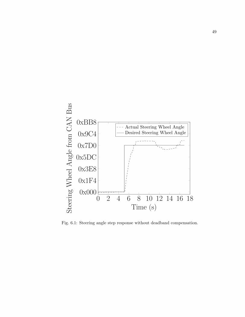
49

0 2 4 6 8 10 12 14 16 180x000

0x1F4

0x3E8

0x5DC

0x7D0

0x9C4

0xBB8

Time (s)

SteeringWheelAnglefrom

CANBus

Actual Steering Wheel AngleDesired Steering Wheel Angle

Fig. 6.1: Steering angle step response without deadband compensation.

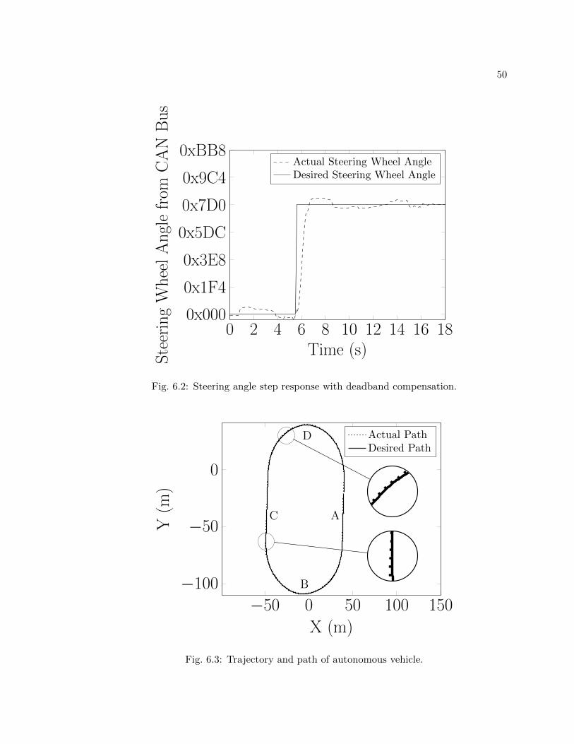
50

0 2 4 6 8 10 12 14 16 180x000

0x1F4

0x3E8

0x5DC

0x7D0

0x9C4

0xBB8

Time (s)

SteeringWheelAnglefrom

CANBus

Actual Steering Wheel AngleDesired Steering Wheel Angle

Fig. 6.2: Steering angle step response with deadband compensation.

−50 0 50 100 150−100

−50

0

A

B

C

D

X (m)

Y(m

)

Actual PathDesired Path

−50 0 50 100 150−100

−50

0

A

B

C

D

X (m)

Y(m

)

Actual PathDesired Path

−50 0 50 100 150−100

−50

0

A

B

C

D

X (m)

Y(m

)

Actual PathDesired Path

Fig. 6.3: Trajectory and path of autonomous vehicle.

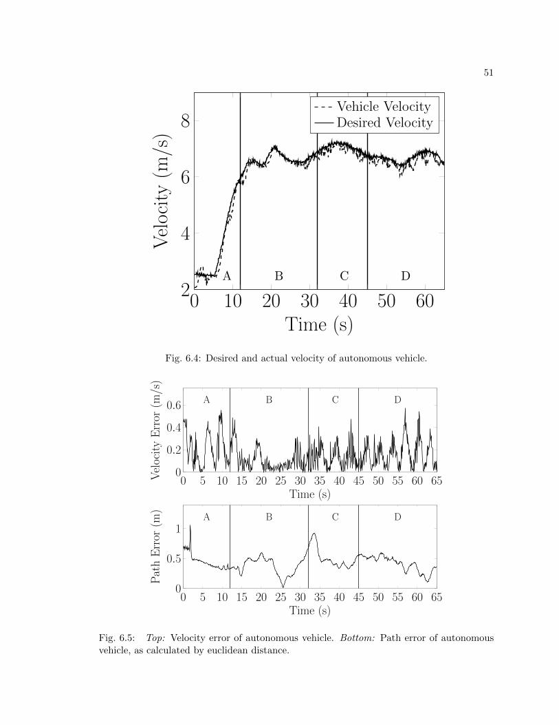
51

0 10 20 30 40 50 602

4

6

8

A B C D

Time (s)

Velocity(m

/s)

Vehicle VelocityDesired Velocity

Fig. 6.4: Desired and actual velocity of autonomous vehicle.

0 5 10 15 20 25 30 35 40 45 50 55 60 650

0.2

0.4

0.6 A B C D

Time (s)

VelocityError

(m/s)

0 5 10 15 20 25 30 35 40 45 50 55 60 650

0.5

1A B C D

Time (s)

PathError

(m)

Fig. 6.5: Top: Velocity error of autonomous vehicle. Bottom: Path error of autonomousvehicle, as calculated by euclidean distance.

52

CHAPTER 7

CONCLUSION

7.1 Conclusion

The platform discussed in this thesis provides an inexpensive open-source vehicle au-

tomation system that takes advantage of the vehicle’s native communication and control

systems to achieve vehicle control. This method was preferred to more expensive and more

intrusive platforms on the market today. The overall cost of the components needed to

automate a stock vehicle was $2,315, the itemized cost breakdown can be seen in Table

7.1. The hardware described in Chapter 5 is available online, and the code used for au-

tomated vehicle testing is available at https://github.com/rajnikant1010/EVAutomation.

This platform will provide a good starting point for automated vehicle research.

The future work opportunities for this project vary in scope and field. First, a more

detailed higher-order model could obtained through a variety of techniques that may better

represent the vehicle. An improved model will improve simulations and aid in the controller

design process. Second, more advanced techniques could be applied to the low-level con-

trollers. The PID approach presented in this thesis is an effective method and is simple to

implement, but other methods could be explored to identify the best approaches. Third,

differential flatness path following controller could be replaced by a variety of path planning

Table 7.1: Itemized Cost Breakdown of Automation PlatformComponent Cost

Swiftnav Piksi RTK-GPS $995PCAN - CAN Bus Analyzer $225TI Tiva C TM4C1294 $20NewMar UPS $495PCB and Components $80Computer $500

TOTAL $2,315

53

controllers to test the effect different controllers have on lateral path accuracy.

The future work planned for this vehicle is dynamic wireless power transfer for in-

motion wireless charging. A group of researchers at Utah State University plan to install a

charging coil under the car for wireless charging. In order to have efficient wireless power

transfer, the lateral path accuracy must be less than ± 7 cm. To achieve this, a computer

vision based lane detection and lane keeping algorithm will be developed and tested on the

test track at the EVR.

54

REFERENCES

[1] M. Casey. Want a self-driving car? look on the driveway. [Online]. Available:http://fortune.com/2014/12/06/autonomous-vehicle-revolution/

[2] E. Guizzo, “How googles self-driving car works,” IEEE Spectrum Online, October,vol. 18, 2011.

[3] R. Rajamani, Vehicle Dynamics and Control, 2nd ed., ser. Mechanical EngineeringSeries. Springer US, 2012.

[4] C. Valasek and C. Miller, “Adventures in automotive networks and control units,”IOActive, Tech. Rep., 2014.

[5] C. Miller and C. Valasek, “Remote exploitation of an unaltered passenger vehicle,”IOActive, Tech. Rep., 2015.

[6] S. Checkoway, D. McCoy, B. Kantor, D. Anderson, H. Shacham, S. Savage, K. Koscher,A. Czeskis, F. Roesner, and T. Kohno, “Comprehensive experimental analyses of au-tomotive attack surfaces.” in USENIX Security Symposium, 2011.

[7] O. C. Onar, J. M. Miller, S. L. Campbell, C. Coomer, C. P. White, and L. E. Seiber,“A novel wireless power transfer for in-motion ev/phev charging,” in Applied PowerElectronics Conference and Exposition (APEC), 2013 Twenty-Eighth Annual IEEE,March 2013, pp. 3073–3080.

[8] Electric vehicle and roadway. Utah State University. [Online]. Available: https://evr.usu.edu/

[9] I. F. Vis, “Survey of research in the design and control of automated guidedvehicle systems,” European Journal of Operational Research, vol. 170, no. 3, pp. 677– 709, 2006. [Online]. Available: http://www.sciencedirect.com/science/article/pii/S0377221704006459

[10] Darpa grand challenge. DARPA. [Online]. Available: http://archive.darpa.mil/grandchallenge04/

[11] Grand challenge ’05. DARPA. [Online]. Available: http://archive.darpa.mil/grandchallenge05/

[12] Urban challenge. DARPA. [Online]. Available: http://archive.darpa.mil/grandchallenge/index.html

[13] C. Englund, L. Chen, J. Ploeg, E. Semsar-Kazerooni, A. Voronov, H. H. Bengtsson, andJ. Didoff, “The grand cooperative driving challenge 2016: boosting the introduction ofcooperative automated vehicles,” IEEE Wireless Communications, vol. 23, no. 4, pp.146–152, August 2016.

55

[14] J. E. A. Dias, G. A. S. Pereira, and R. M. Palhares, “Longitudinal model identifi-cation and velocity control of an autonomous car,” IEEE Transactions on IntelligentTransportation Systems, vol. 16, no. 2, pp. 776–786, April 2015.

[15] Ros. [Online]. Available: https://www.ros.org

[16] J. Ferrin, R. Leishman, R. Beard, and T. McLain, “Differential flatness based controlof a rotorcraft for aggressive maneuvers,” in 2011 IEEE/RSJ International Conferenceon Intelligent Robots and Systems, Sept 2011, pp. 2688–2693.

[17] K. Koscher, A. Czeskis, F. Roesner, S. Patel, T. Kohno, S. Checkoway, D. McCoy,B. Kantor, D. Anderson, H. Shacham et al., “Experimental security analysis of amodern automobile,” in 2010 IEEE Symposium on Security and Privacy. IEEE,2010, pp. 447–462.

[18] “Road vehicles - controller area network (can) - part 1: Data link layer and physicalsignalling,” International Organization for Standardization, Geneva, CH, standard,2015.

[19] Wiring Diagrams: Focus Electric 2013, Ford Motor Company.

[20] EBSCOhost, “Auto repair reference center,” https://www.ebscohost.com/public/auto-repair-reference-center, Tech. Rep., 2013.

[21] Ecu analysis with canalyzer. Vector. [Online]. Available: https://vector.com/vi canalyzer en.html

[22] Pcan-usb. [Online]. Available: http://www.peak-system.com/PCAN-USB.199.0.html?L=1

[23] Arm cortex-m4f based mcu tm4c1294 connected launchpad. Texas Instruments.[Online]. Available: http://www.ti.com/tool/ek-tm4c1294xl

[24] Sn65hvd230. Texas Instruments. [Online]. Available: http://www.ti.com/product/SN65HVD230

[25] Active park assist. Ford Motor Company. [Online]. Available: https://owner.ford.com/how-tos/vehicle-features/convenience-and-comfort/active-park-assist.html

[26] O. Persson and G. Persson, “Torque sensor for automotive applicaitons.” [Online].Available: http://www.iea.lth.se/publications/MS-Theses/Full%20document/5352full document.pdf

[27] Obd-ii background. B&B Electronics. [Online]. Available: http://www.obdii.com/background.html

[28] P. S. Murvay and B. Groza, “Source identification using signal characteristics in con-troller area networks,” IEEE Signal Processing Letters, vol. 21, no. 4, pp. 395–399,April 2014.

56

[29] K.-T. Cho and K. G. Shin, “Fingerprinting electronic control units for vehicle intrusiondetection,” in 25th USENIX Security Symposium (USENIX Security 16). USENIXAssociation, 2016, pp. 911–927.

[30] Md-awd-150. Mustang Dynamometer. [Online]. Available: https://mustangdyne.com/md-awd-150/

[31] E. D. B. Medagoda and P. W. Gibbens, “Synthetic-waypoint guidance algorithmfor following a desired flight trajectory,” Journal of Guidance, Control, andDynamics, vol. 33, no. 2, pp. 601–606, 2016/11/21 2010. [Online]. Available:http://dx.doi.org/10.2514/1.46204

[32] R. C. Coulter, “Implementation of the pure pursuit path tracking algorithm,” DTICDocument, Tech. Rep., 1992.

[33] J. Villagra, D. Herrero-Perez, and M. Abderrahim, “Robust flatness-based control of anagv under varying load and friction conditions,” in 2009 IEEE International Conferenceon Control and Automation. IEEE, 2009, pp. 1621–1628.

[34] G. G. Rigatos, Nonlinear Control and Filtering Using Differential Flatness Approaches:Applications to Electromechanical Systems. Springer Publishing Company, Incorpo-rated, 2015.

[35] G. Rigatos, Nonlinear Control and Filtering Using Differential Flatness Approaches,1st ed., ser. Studies in Systems, Decision and Control. Springer International Pub-lishing, 2015, vol. 25.

[36] Original piksi rtk kit (915 mhz). [Online]. Available: http://store.swiftnav.com/s.nl/it.A/id.4216/.f

[37] Newmar powering the mobile network. NewMar. [Online]. Avail-able: http://newmarpower.com/wp-content/uploads/2016/04/Newmar Powering theMobile Network Mobile Catalog 2015-Web.pdf

[38] Sn65hvd230 can board. WaveShare. [Online]. Available: http://www.waveshare.com/sn65hvd230-can-board.htm

[39] R. B. Langley, “Rtk gps,” GPS World, vol. 9, no. 9, pp. 70–76, 1998.

[40] E. Kaplan and C. Hegarty, Understanding GPS: Principles and Applications, ser.Artech House mobile communications series. Artech House, 2006. [Online]. Available:https://books.google.com/books?id=V 5OAAAAMAAJ

[41] Tivaware™for c series (complete). Texas Instruments. [Online]. Available: http://www.ti.com/tool/sw-tm4c

[42] Ros tutorials. [Online]. Available: wiki.ros.org/ROS/Tutorials