PLASTIC DEFORMATIONPLASTIC DEFORMATION

Modes of Deformation

The Uniaxial Tension Test

Mechanisms underlying Plastic Deformation

Strengthening mechanisms

Mechanical MetallurgyGeorge E Dieter

McGraw-Hill Book Company, London (1988)

MATERIALS SCIENCEMATERIALS SCIENCE&&

ENGINEERING ENGINEERING

Anandh Subramaniam & Kantesh Balani

Materials Science and Engineering (MSE)

Indian Institute of Technology, Kanpur- 208016

Email: anandh@iitk.ac.in, URL: home.iitk.ac.in/~anandh

AN INTRODUCTORY E-BOOKAN INTRODUCTORY E-BOOK

Part of

http://home.iitk.ac.in/~anandh/E-book.htmhttp://home.iitk.ac.in/~anandh/E-book.htm

A Learner’s GuideA Learner’s GuideA Learner’s GuideA Learner’s Guide

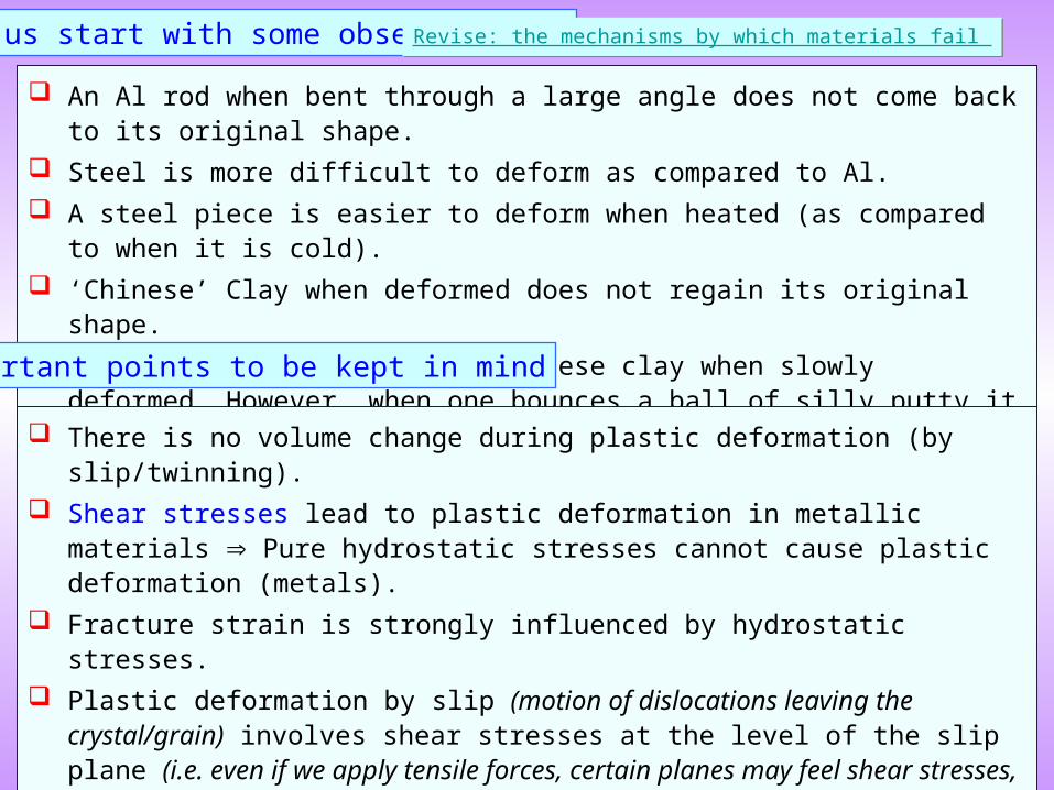
An Al rod when bent through a large angle does not come back to its original shape.

Steel is more difficult to deform as compared to Al.

A steel piece is easier to deform when heated (as compared to when it is cold).

‘Chinese’ Clay when deformed does not regain its original shape.

‘Silly putty’ deforms like Chinese clay when slowly deformed. However, when one bounces a ball of silly putty it bounces like a rubber ball.

Let us start with some observations… Revise: the mechanisms by which materials fail Revise: the mechanisms by which materials fail

There is no volume change during plastic deformation (by slip/twinning).

Shear stresses lead to plastic deformation in metallic materials Pure hydrostatic stresses cannot cause plastic deformation (metals).

Fracture strain is strongly influenced by hydrostatic stresses.

Plastic deformation by slip (motion of dislocations leaving the crystal/grain) involves shear stresses at the level of the slip plane (i.e. even if we apply tensile forces, certain planes may feel shear stresses, which can lead to slip).

Amorphous materials can deform by ‘flow’ (e.g. glass blowing of heated glass), etc. → these are not the focus of the current chapter.

Important points to be kept in mind

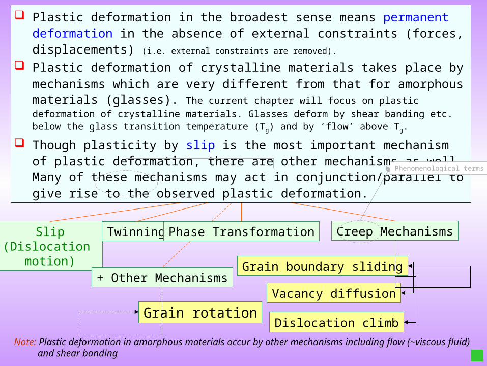
Slip(Dislocation

motion)

Plastic Deformation in Crystalline Materials

Twinning Phase Transformation Creep Mechanisms

Grain boundary sliding

Vacancy diffusion

Dislocation climb

+ Other Mechanisms

Note: Plastic deformation in amorphous materials occur by other mechanisms including flow (~viscous fluid) and shear banding

Plastic deformation in the broadest sense means permanent deformation in the absence of external constraints (forces, displacements) (i.e. external constraints are removed).

Plastic deformation of crystalline materials takes place by mechanisms which are very different from that for amorphous materials (glasses). The current chapter will focus on plastic deformation of crystalline materials. Glasses deform by shear banding etc. below the glass transition temperature (Tg) and by ‘flow’ above Tg.

Though plasticity by slip is the most important mechanism of plastic deformation, there are other mechanisms as well. Many of these mechanisms may act in conjunction/parallel to give rise to the observed plastic deformation.

Grain rotation

Phenomenological terms

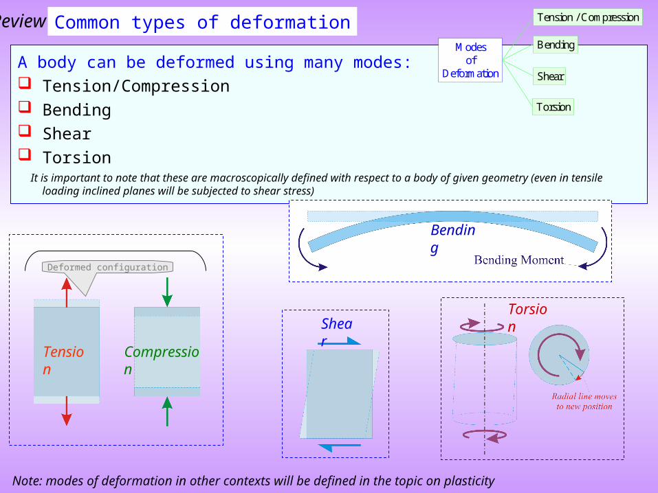
A body can be deformed using many modes: Tension/Compression Bending Shear Torsion It is important to note that these are macroscopically defined with respect to a body of given geometry (even in tensile loading inclined

planes will be subjected to shear stress)

Common types of deformation

Tension

Compression

Shear

Torsion

Deformed configuration

Bending

Note: modes of deformation in other contexts will be defined in the topic on plasticity

Tension / Compression

Torsion

Modesof

Deformation Shear

Bending

Review

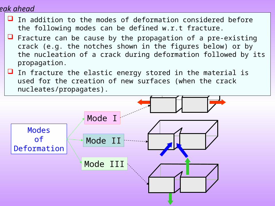
Mode I

Mode III

Modesof

DeformationMode II

In addition to the modes of deformation considered before the following modes can be defined w.r.t fracture.

Fracture can be cause by the propagation of a pre-existing crack (e.g. the notches shown in the figures below) or by the nucleation of a crack during deformation followed by its propagation.

In fracture the elastic energy stored in the material is used for the creation of new surfaces (when the crack nucleates/propagates).

Peak ahead

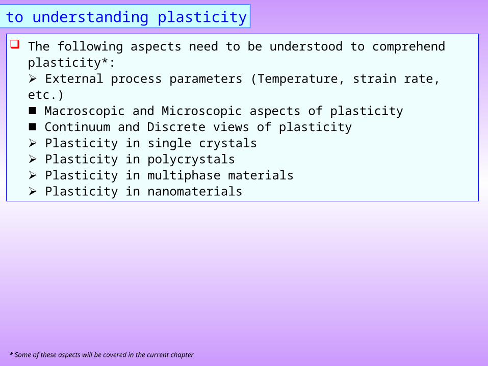
The following aspects need to be understood to comprehend plasticity*: External process parameters (Temperature, strain rate, etc.) Macroscopic and Microscopic aspects of plasticity Continuum and Discrete views of plasticity Plasticity in single crystals Plasticity in polycrystals Plasticity in multiphase materials Plasticity in nanomaterials

Path to understanding plasticity

* Some of these aspects will be covered in the current chapter

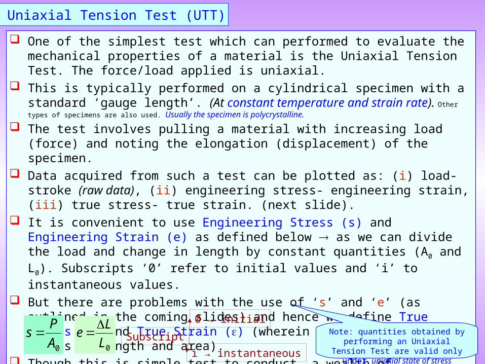
One of the simplest test which can performed to evaluate the mechanical properties of a material is the Uniaxial Tension Test. The force/load applied is uniaxial.

This is typically performed on a cylindrical specimen with a standard ‘gauge length’. (At constant temperature and strain rate). Other types of specimens are also used. Usually the specimen is polycrystalline.

The test involves pulling a material with increasing load (force) and noting the elongation (displacement) of the specimen.

Data acquired from such a test can be plotted as: (i) load-stroke (raw data), (ii) engineering stress- engineering strain, (iii) true stress- true strain. (next slide).

It is convenient to use Engineering Stress (s) and Engineering Strain (e) as defined below as we can divide the load and change in length by constant quantities (A0 and L0). Subscripts ‘0’ refer to initial values and ‘i’ to instantaneous values.

But there are problems with the use of ‘s’ and ‘e’ (as outlined in the coming slides) and hence we define True Stress () and True Strain () (wherein we use instantaneous values of length and area).

Though this is simple test to conduct, a wealth of information about the mechanical behaviour of a material can be obtained (Modulus of elasticity, ductility etc.) However, it must be cautioned that this data should be used with caution under other states of stress.

The Uniaxial Tension Test (UTT)

0A

Ps

0L

Le

0 → initial

i → instantaneous

SubscriptNote: quantities obtained by performing an Uniaxial Tension Test are valid only under

uniaxial state of stress

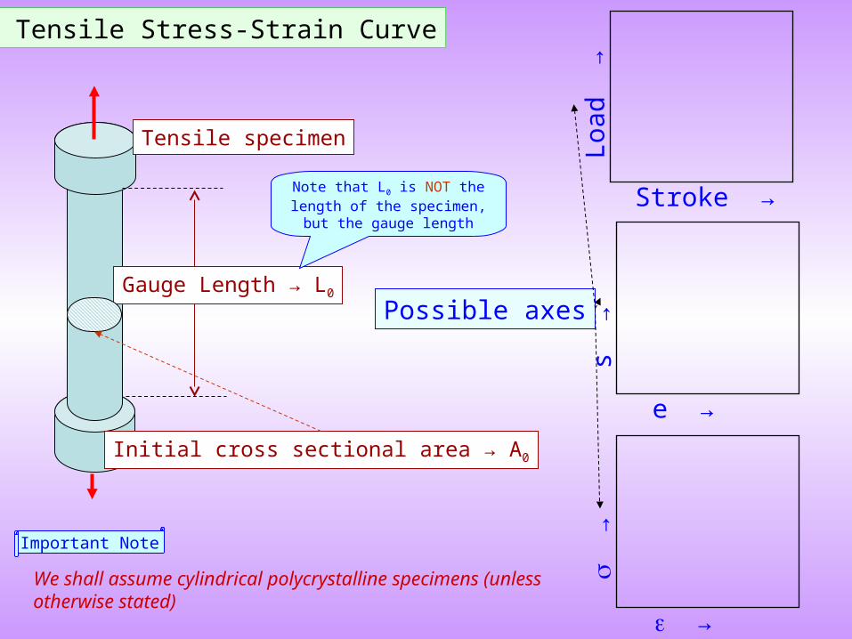
The Tensile Stress-Strain Curve

Stroke →

Loa

d →

e →

s →

→

→

Gauge Length → L0

Possible axes

Tensile specimen

Initial cross sectional area → A0

Important Note

We shall assume cylindrical polycrystalline specimens (unless otherwise stated)

Note that L0 is NOT the length of the specimen, but the gauge length

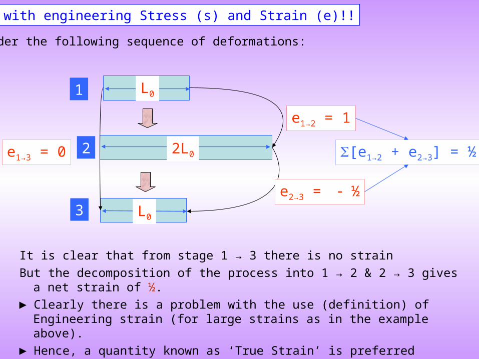
Problem with engineering Stress (s) and Strain (e)!!

Consider the following sequence of deformations:

L0

2L0

L0

e1→2 = 1

e2→3 = ½

e1→3 = 0

1

2

3

[e1→2 + e2→3] = ½

It is clear that from stage 1 → 3 there is no strain

But the decomposition of the process into 1 → 2 & 2 → 3 gives a net strain of ½.

► Clearly there is a problem with the use (definition) of Engineering strain (for large strains as in the example above).

► Hence, a quantity known as ‘True Strain’ is preferred (along with True Stress) as defined in the next slide.

True Stress () and Strain ()

iA

P

0

ln0

L

L

L

dLL

L

0A

Ps

0L

Le

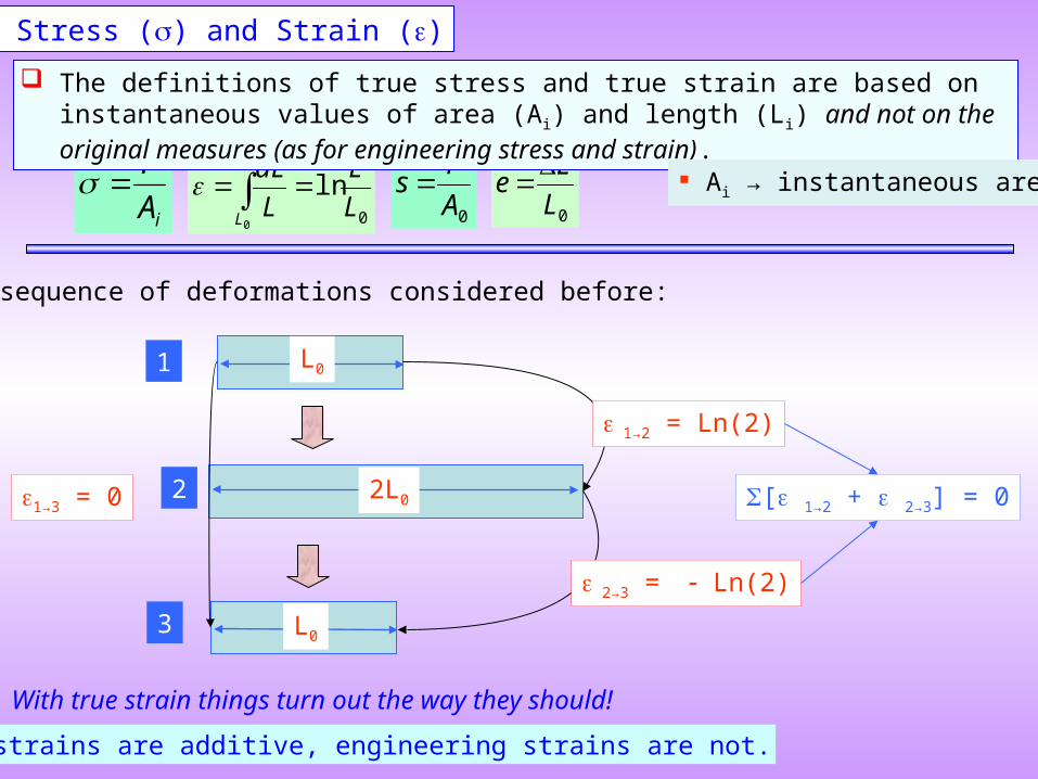
The definitions of true stress and true strain are based on instantaneous values of area (A i) and length (Li) and not on the original measures (as for engineering stress and strain).

Ai → instantaneous area

Same sequence of deformations considered before:

L0

2L0

L0

1→2 = Ln(2)

2→3 = Ln(2)

1→3 = 0

1

2

3

[ 1→2 + 2→3] = 0

With true strain things turn out the way they should!

True strains are additive, engineering strains are not.

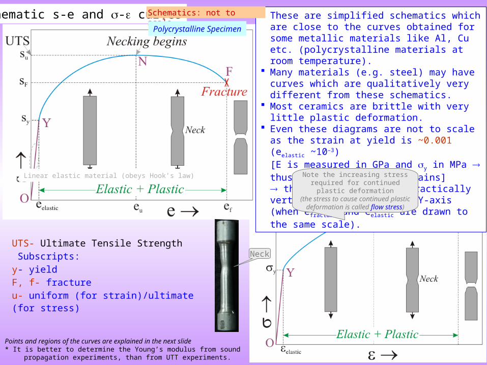
Schematic s-e and - curves

Points and regions of the curves are explained in the next slide * It is better to determine the Young’s modulus from sound propagation experiments,

than from UTT experiments.

These are simplified schematics which are close to the curves obtained for some metallic materials like Al, Cu etc. (polycrystalline materials at room temperature).

Many materials (e.g. steel) may have curves which are qualitatively very different from these schematics.

Most ceramics are brittle with very little plastic deformation.

Even these diagrams are not to scale as the strain at yield is ~0.001 (eelastic ~10–3)[E is measured in GPa and y in MPa thus giving this small strains] the linear portion is practically vertical and stuck to the Y-axis (when efracture and eelastic are drawn to the same scale).

Schematics: not to scale

Note the increasing stress required for continued plastic deformation

(the stress to cause continued plastic deformation is called flow stress)

Neck

Polycrystalline Specimen

Linear elastic material (obeys Hook’s law)

UTS- Ultimate Tensile Strength Subscripts: y- yield F, f- fracture u- uniform (for strain)/ultimate (for stress)

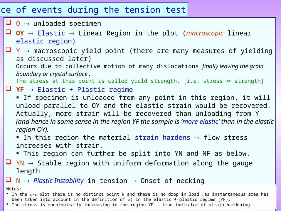
O unloaded specimen OY Elastic Linear Region in the plot (macroscopic linear elastic region) Y macroscopic yield point (there are many measures of yielding as discussed later)

Occurs due to collective motion of many dislocations finally leaving the grain boundary or crystal surface.The stress at this point is called yield strength. [i.e. stress strength]

YF Elastic + Plastic regime If specimen is unloaded from any point in this region, it will unload parallel to OY and the elastic strain would be recovered. Actually, more strain will be recovered than unloading from Y (and hence in some sense in the region YF the sample is ‘more elastic’ than in the elastic region OY). In this region the material strain hardens flow stress increases with strain. This region can further be split into YN and NF as below.

YN Stable region with uniform deformation along the gauge length N Plastic Instability in tension Onset of necking

True condition of uniaxiality broken onset of triaxial state of stress (loading remains uniaxial but the state of stress in the cylindrical specimen is not).

NF most of the deformation is localized at the neck Specimen in a triaxial state of stress

F Fracture of specimen (many polycrystalline materials like Al show cup and cone fracture)

Sequence of events during the tension test

Notes: In the - plot there is no distinct point N and there is no drop in load (as instantaneous area has been taken into account in the definition of ) in the

elastic + plastic regime (YF). The stress is monotonically increasing in the region YF true indicator of strain hardening.

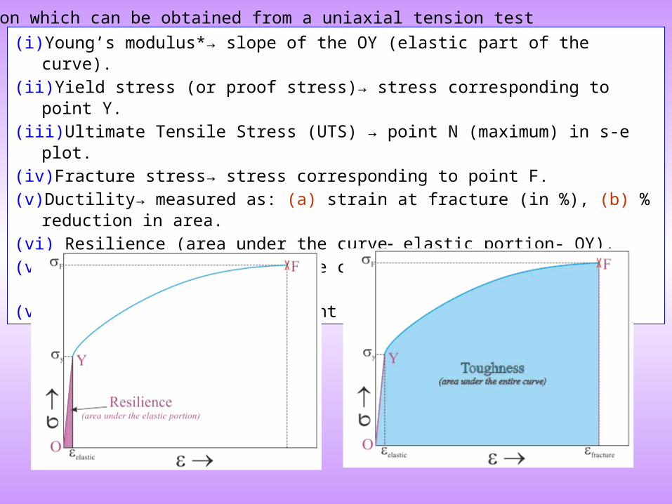
(i) Young’s modulus*→ slope of the OY (elastic part of the curve).

(ii) Yield stress (or proof stress)→ stress corresponding to point Y.

(iii) Ultimate Tensile Stress (UTS) → point N (maximum) in s-e plot.

(iv) Fracture stress→ stress corresponding to point F.

(v) Ductility→ measured as: (a) strain at fracture (in %), (b) % reduction in area.

(vi) Resilience (area under the curve elastic portion- OY).

(vii) Toughness (area under the curve total)→ has unit of Energy/volume [J/m3].

(viii) Strain hardening exponent (from - plot).

Information which can be obtained from a uniaxial tension test

Q & A What is meant by toughness?

Toughness is the energy absorbed by the material upto failure. This could be in a uniaxial tension test or in an impact test (which is done using a notched specimen Charpy or Izod specimens).

Toughness is combined parameter involving strength and ductility (i.e. a material with higher strength for a given ductility or higher ductility for a given strength has higher toughness).

Q & A What are the simple tests we can perform on test specimens to evaluate their mechanical behaviour?

Uniaxial tension test. Compression test. Hardness test. Bending test (3-point, 4-point bend tests). Torsion test.

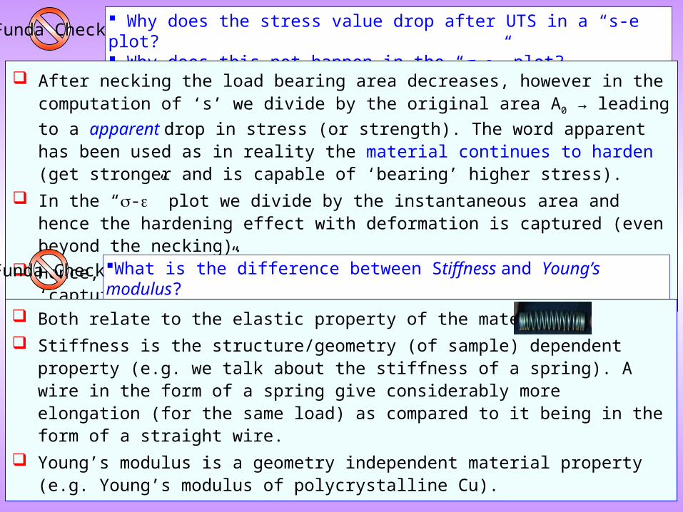
Why does the stress value drop after UTS in a “s-e” plot? Why does this not happen in the “-” plot?

Funda Check

After necking the load bearing area decreases, however in the computation of ‘s’ we divide by the original area A0 → leading to a apparent drop in stress (or strength). The word

apparent has been used as in reality the material continues to harden (get stronger and is capable of ‘bearing’ higher stress).

In the “-” plot we divide by the instantaneous area and hence the hardening effect with deformation is captured (even beyond the necking).

Hence, in the “-” plot the necking event cannot be ‘captured’.

What is the difference between Stiffness and Young’s modulus?Funda Check

Both relate to the elastic property of the material.

Stiffness is the structure/geometry (of sample) dependent property (e.g. we talk about the stiffness of a spring). A wire in the form of a spring give considerably more elongation (for the same load) as compared to it being in the form of a straight wire.

Young’s modulus is a geometry independent material property (e.g. Young’s modulus of polycrystalline Cu).

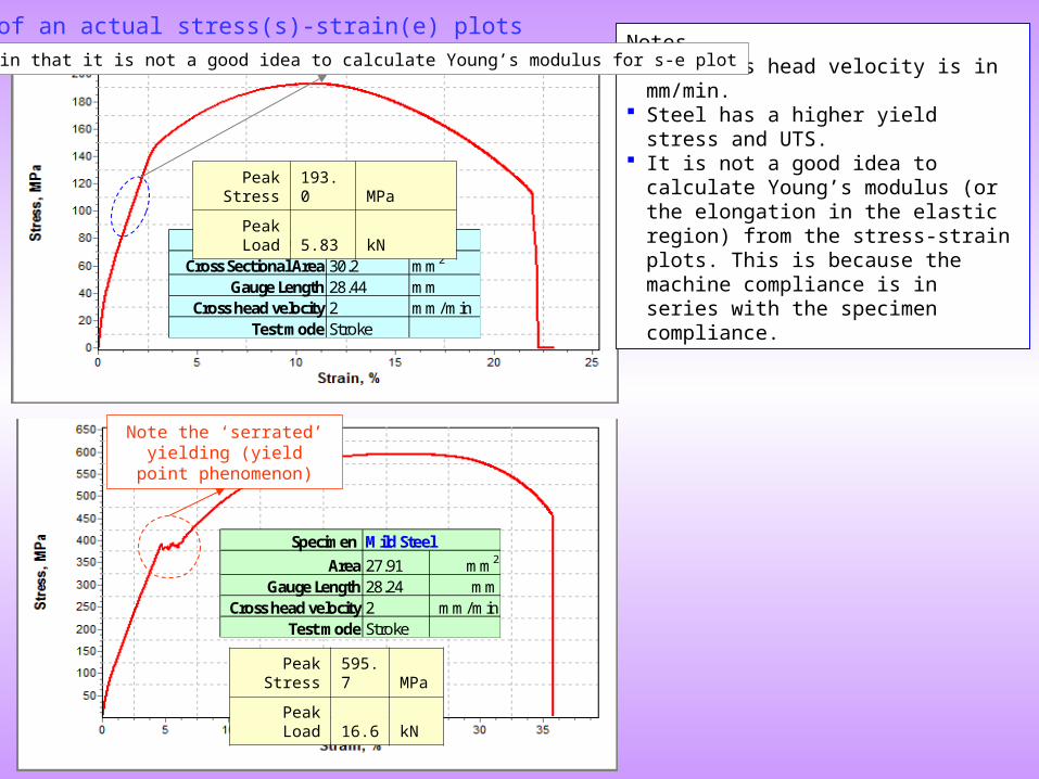
Specimen ID AluminiumCross Sectional Area 30.2 mm2

Gauge Length 28.44 mmCross head velocity 2 mm/min

Test mode Stroke

Peak Stress 193.0 MPa

Peak Load 5.83 kN

Specimen Mild SteelArea 27.91 mm2

Gauge Length 28.24 mmCross head velocity 2 mm/min

Test mode Stroke

Note the ‘serrated’ yielding (yield point phenomenon)

Peak Stress 595.7 MPa

Peak Load 16.6 kN

Result of an actual stress(s)-strain(e) plotsNotes The cross head velocity is in mm/min. Steel has a higher yield stress and UTS. It is not a good idea to calculate Young’s

modulus (or the elongation in the elastic region) from the stress-strain plots. This is because the machine compliance is in series with the specimen compliance.

Note again that it is not a good idea to calculate Young’s modulus for s-e plot

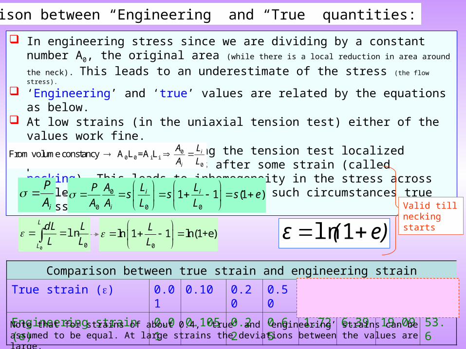
Comparison between true strain and engineering strain

True strain () 0.01 0.10 0.20 0.50 1.0 2.0 3.0 4.0

Engineering strain (e) 0.01 0.105 0.22 0.65 1.72 6.39 19.09 53.6

e)(ε 1ln

e)s( 1

Comparison between “Engineering” and “True” quantities:

Note that for strains of about 0.4, ‘true’ and ‘engineering’ strains can be assumed to be equal. At large strains the deviations between the values are large.

In engineering stress since we are dividing by a constant number A0, the original area (while

there is a local reduction in area around the neck). This leads to an underestimate of the stress (the flow stress).

‘Engineering’ and ‘true’ values are related by the equations as below. At low strains (in the uniaxial tension test) either of the values work fine. As we shall see that during the tension test localized plastic deformation occurs after some

strain (called necking). This leads to inhomogeneity in the stress across the length of the sample and under such circumstances true stress should be used.

iA

P

0

ln0

L

L

L

dLL

L

0

ln 1 1 ln(1+e)L

L

0

0 0 0

1 1 (1 )i i

i

A L LPs s s e

A A L L

00 0 i i

0

From volume constancy A L =A L i

i

A L

A L

Valid till necking starts

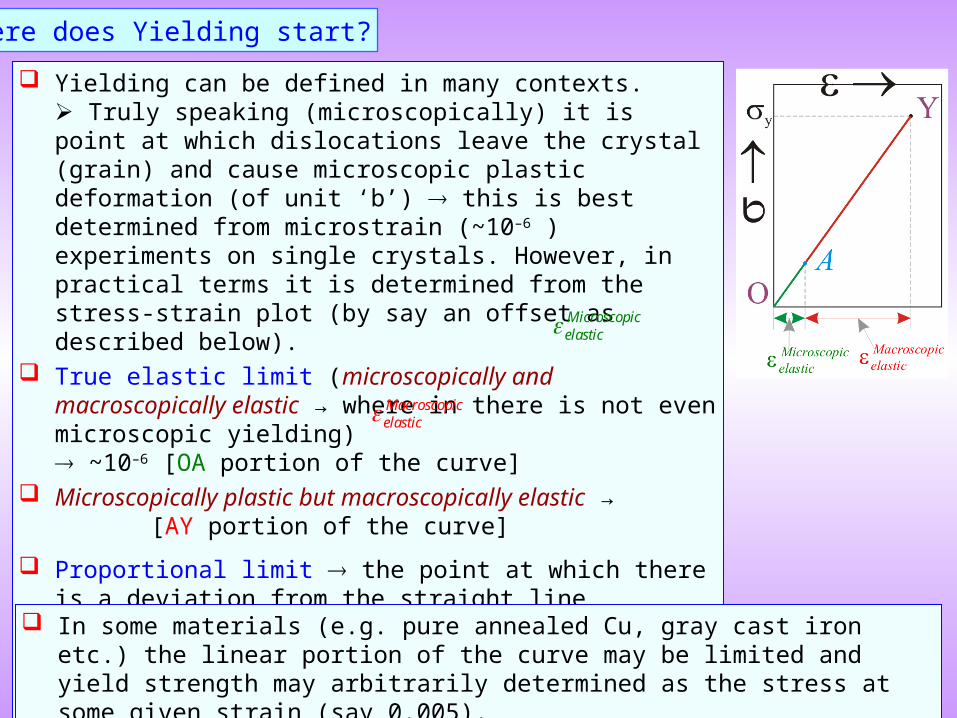
Yielding can be defined in many contexts. Truly speaking (microscopically) it is point at which dislocations leave the crystal (grain) and cause microscopic plastic deformation (of unit ‘b’) this is best determined from microstrain (~10–6 ) experiments on single crystals. However, in practical terms it is determined from the stress-strain plot (by say an offset as described below).

True elastic limit (microscopically and macroscopically elastic → where in there is not even microscopic yielding) ~10–6 [OA portion of the curve]

Microscopically plastic but macroscopically elastic →[AY portion of the curve]

Proportional limit the point at which there is a deviation from the straight line ‘elastic’ regime

Offset Yield Strength (proof stress) A curve is drawn parallel to the elastic line at a given strain like 0.2% (= 0.002) to determine the yield strength.

Where does Yielding start?

In some materials (e.g. pure annealed Cu, gray cast iron etc.) the linear portion of the curve may be limited and yield strength may arbitrarily determined as the stress at some given strain (say 0.005).

Microscopicelastic

Macroscopicelastic

Important Points

Yielding begins when a stress equal to y (yield stress) is applied; however to cause further plastic deformation increased stress has to be applied i.e. the material hardens with plastic deformation → known as work hardening/strain hardening.

Beyond necking the state of stress becomes triaxial (in a cylindrical specimen considered). Technically the yield criterion in uniaxial tension cannot be applied beyond this point.

We shall keep our focus on plastic deformation by slip. y is yield stress in an uniaxial tension test (i.e. plastic deformation will start after crossing yield stress

only under uniaxial tensile loading) and should not be used in other states of stress (other criteria of yield should be used for a generalized state of stress).

I.e in uniaxial tension the yield criterion is very simple:Yielding starts when: y .

Hydrostatic pressure (leading to hydrostatic stress in a material) does not lead to yielding in a continuous solid (usually!). This implies that the stress deviator holds the key to yielding.

For an isotropic material the yield criterion will not be independent of the choice of the axes (i.e. a invariant function). Hence, for an isotropic material the yield criteria (we will note that there are more than

one) will be a function of the invariants of the stress deviator.

Two commonly yield criteria are: Von Mices or Distortion-Energy Criterion Maximum shear stress or Tresca Criterion. (We will consider these later).

Plastic deformation (= yielding) and state of stress

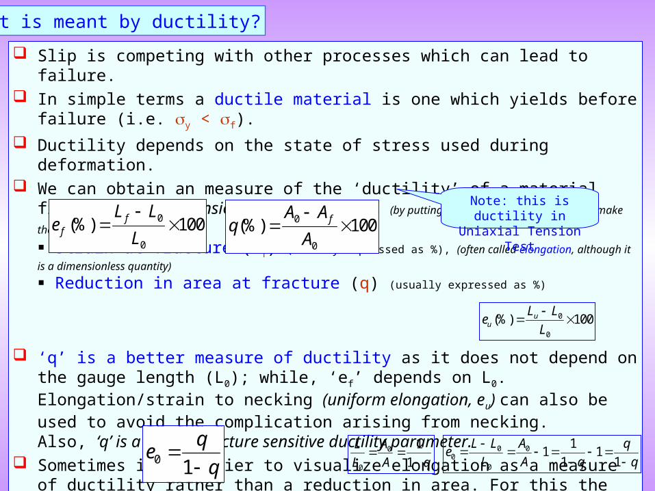
Slip is competing with other processes which can lead to failure. In simple terms a ductile material is one which yields before failure (i.e. y < f).

Ductility depends on the state of stress used during deformation. We can obtain an measure of the ‘ductility’ of a material from the uniaxial tension test as

follows (by putting together the fractured parts to make the measurement): Strain at fracture (ef) (usually expressed as %), (often called elongation, although it is a dimensionless quantity)

Reduction in area at fracture (q) (usually expressed as %)

‘q’ is a better measure of ductility as it does not depend on the gauge length (L0); while, ‘ef’ depends on L0. Elongation/strain to necking (uniform elongation, eu) can also be used to avoid the complication arising from necking.Also, ‘q’ is a ‘more’ structure sensitive ductility parameter.

Sometimes it is easier to visualize elongation as a measure of ductility rather than a reduction in area. For this the calculation has to be based on a very short gauge length in the necked region called Zero-gauge-length elongation (e0). ‘e0’ can be calculated from ‘q’ using constancy of volume in plastic deformation (AL=A0L0).

What is meant by ductility?

0

0

(%) 100ff

L Le

L

0

0

(%) 100fA Aq

A

Note: this is ductility in Uniaxial Tension Test

0

0

(%) 100uu

L Le

L

0

0

1

1

AL

L A q

0 0

00

11 1

1 1

L L A qe

L A q q

0 1

qe

q

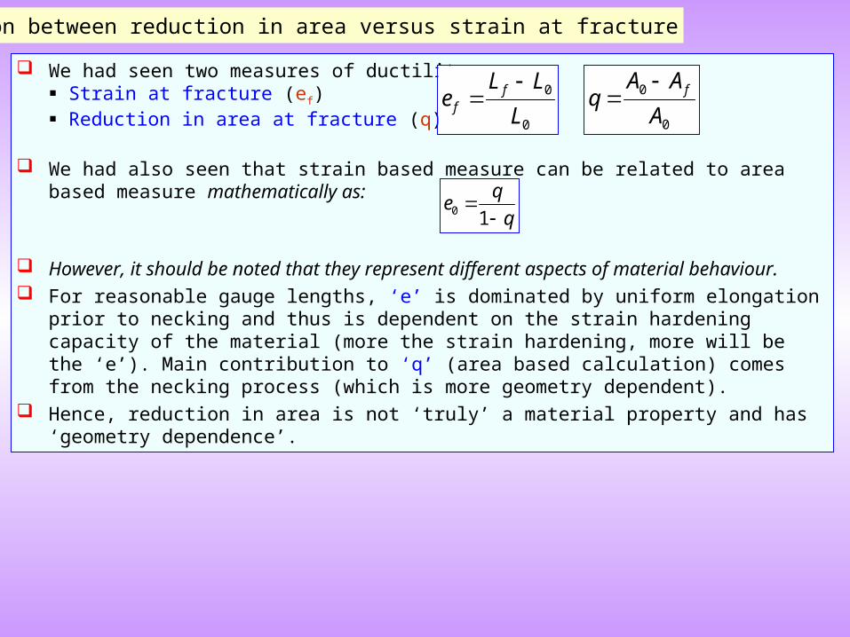
We had seen two measures of ductility: Strain at fracture (ef) Reduction in area at fracture (q)

We had also seen that strain based measure can be related to area based measure mathematically as:

However, it should be noted that they represent different aspects of material behaviour. For reasonable gauge lengths, ‘e’ is dominated by uniform elongation prior to necking and thus is

dependent on the strain hardening capacity of the material (more the strain hardening, more will be the ‘e’). Main contribution to ‘q’ (area based calculation) comes from the necking process (which is more geometry dependent).

Hence, reduction in area is not ‘truly’ a material property and has ‘geometry dependence’.

Comparison between reduction in area versus strain at fracture

0

0

ff

L Le

L

0

0

fA Aq

A

0 1

qe

q

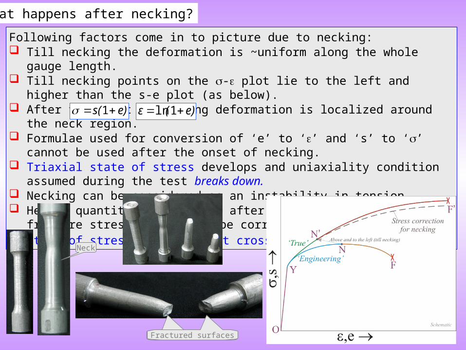
What happens after necking?

Following factors come in to picture due to necking: Till necking the deformation is ~uniform along the whole gauge length. Till necking points on the - plot lie to the left and higher than the s-e plot (as below). After the onset of necking deformation is localized around the neck region. Formulae used for conversion of ‘e’ to ‘’ and ‘s’ to ‘’ cannot be used after the onset of

necking. Triaxial state of stress develops and uniaxiality condition assumed during the test breaks

down. Necking can be considered as an instability in tension. Hence, quantities calculated after the onset of necking (like fracture stress, F) has to be

corrected for: (i) triaxial state of stress, (ii) correct cross sectional area.

e)(ε 1lne)s( 1

Fractured surfacesFractured surfaces

Neck

Beyond necking

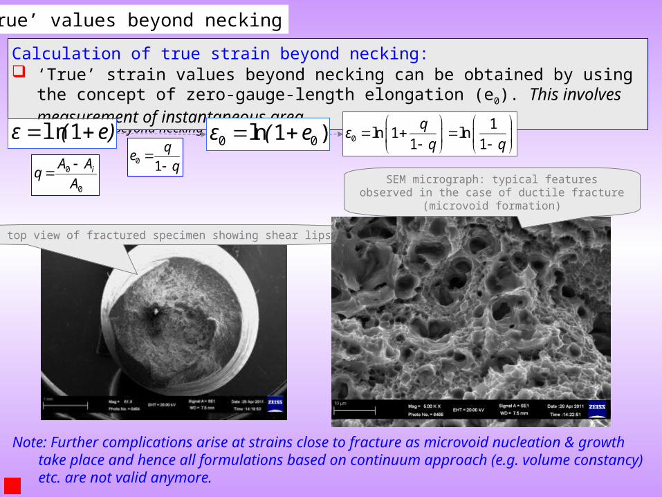
‘True’ values beyond necking

Calculation of true strain beyond necking: ‘True’ strain values beyond necking can be obtained by using the concept of zero-gauge-

length elongation (e0). This involves measurement of instantaneous area.

e)(ε 1ln0 1

qe

q

0

0

iA Aq

A

0 0ln 1 )ε ( e 0

1ln 1 ln

1 1

qε

q q

Note: Further complications arise at strains close to fracture as microvoid nucleation & growth take place and hence all formulations based on continuum approach (e.g. volume constancy) etc. are not valid anymore.

SEM top view of fractured specimen showing shear lips

SEM micrograph: typical features observed in the case of ductile fracture (microvoid formation)

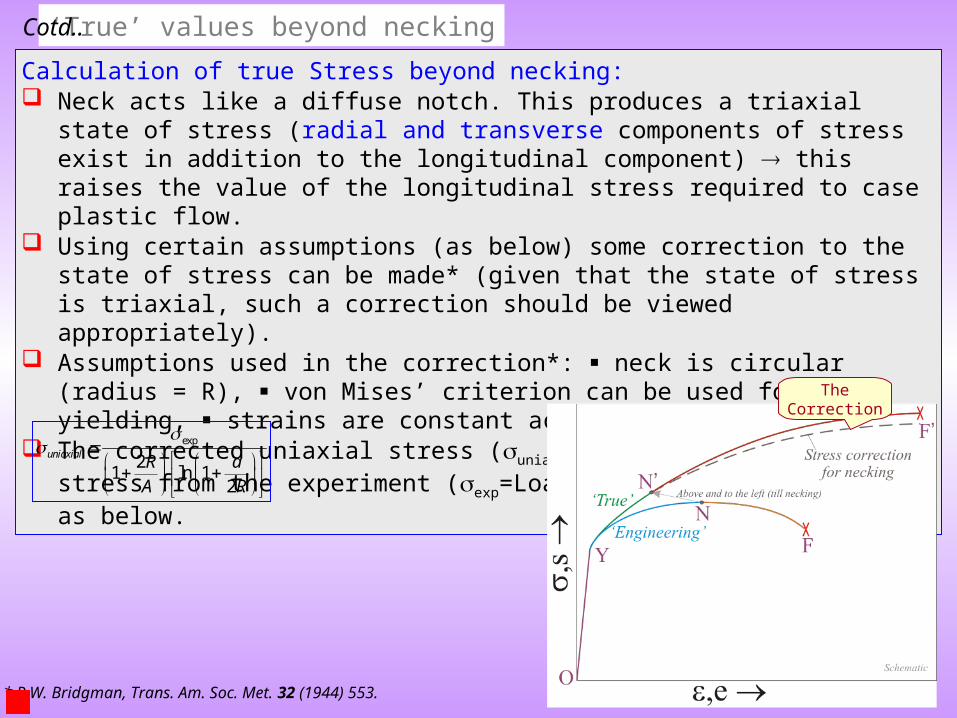
‘True’ values beyond necking

Calculation of true Stress beyond necking: Neck acts like a diffuse notch. This produces a triaxial state of stress (radial and transverse

components of stress exist in addition to the longitudinal component) this raises the value of the longitudinal stress required to case plastic flow.

Using certain assumptions (as below) some correction to the state of stress can be made* (given that the state of stress is triaxial, such a correction should be viewed appropriately).

Assumptions used in the correction*: neck is circular (radius = R), von Mises’ criterion can be used for yielding, strains are constant across the neck.

The corrected uniaxial stress (uniaxial) is calculated from the stress from the experiment (exp=Load/Alocal), using the formula as below.

* P.W. Bridgman, Trans. Am. Soc. Met. 32 (1944) 553.

exp

21 ln 1

2

uniaxialR aA R

The Correction

Cotd..

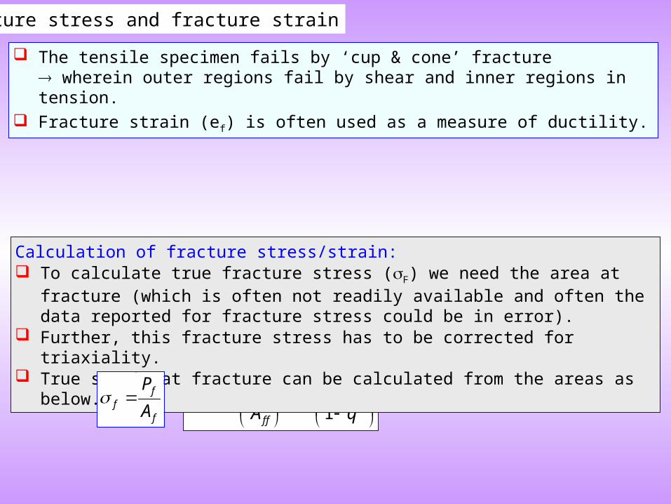
0 1ln ln

1ff f

A

A q

Calculation of fracture stress/strain: To calculate true fracture stress (F) we need the area at fracture (which is often not readily

available and often the data reported for fracture stress could be in error). Further, this fracture stress has to be corrected for triaxiality. True strain at fracture can be calculated from the areas as below.

Fracture stress and fracture strain

The tensile specimen fails by ‘cup & cone’ fracture wherein outer regions fail by shear and inner regions in tension.

Fracture strain (ef) is often used as a measure of ductility.

ff

f

P

A

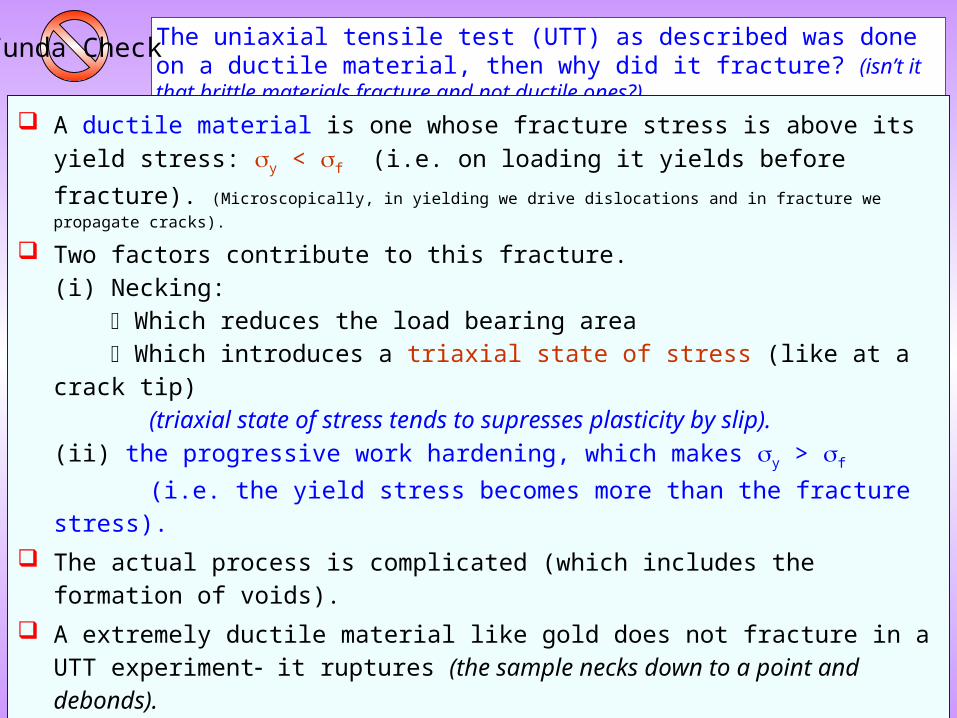
The uniaxial tensile test (UTT) as described was done on a ductile material, then why did it fracture? (isn’t it that brittle materials fracture and not ductile ones?)

Funda Check

A ductile material is one whose fracture stress is above its yield stress: y < f (i.e. on

loading it yields before fracture). (Microscopically, in yielding we drive dislocations and in fracture we propagate

cracks).

Two factors contribute to this fracture.(i) Necking: Which reduces the load bearing area Which introduces a triaxial state of stress (like at a crack tip)

(triaxial state of stress tends to supresses plasticity by slip).

(ii) the progressive work hardening, which makes y > f

(i.e. the yield stress becomes more than the fracture stress).

The actual process is complicated (which includes the formation of voids).

A extremely ductile material like gold does not fracture in a UTT experiment it ruptures (the sample necks down to a point and debonds).

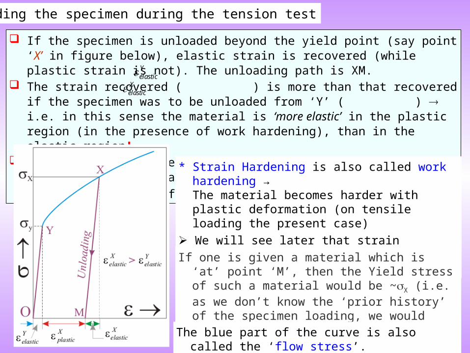
Unloading the specimen during the tension test

If the specimen is unloaded beyond the yield point (say point ‘X’ in figure below), elastic strain is recovered (while plastic strain is not). The unloading path is XM.

The strain recovered ( ) is more than that recovered if the specimen was to be unloaded from ‘Y’ ( ) i.e. in this sense the material is ‘more elastic’ in the plastic region (in the presence of work hardening), than in the elastic region!

If the specimen is reloaded it will follow the reverse path and yielding will start at ~X.

Because of strain hardening* the yield strength of the specimen is higher.

Xelastic

Yelastic

* Strain Hardening is also called work hardening →The material becomes harder with plastic deformation (on tensile loading the present case)

We will see later that strain hardening is usually caused by multiplication of dislocations.

If one is given a material which is ‘at’ point ‘M’, then the Yield stress of such a material would be ~X (i.e. as we don’t know the ‘prior history’ of the specimen loading, we would call ~X as yield stress of the specimen).

The blue part of the curve is also called the ‘flow stress’.

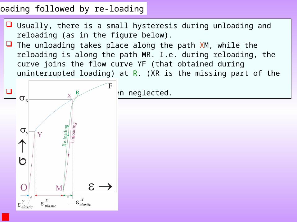
Unloading followed by re-loading

Usually, there is a small hysteresis during unloading and reloading (as in the figure below). The unloading takes place along the path XM, while the reloading is along the path MR.

I.e. during reloading, the curve joins the flow curve YF (that obtained during uninterrupted loading) at R. (XR is the missing part of the flow curve YF).

This hysteresis is often neglected.

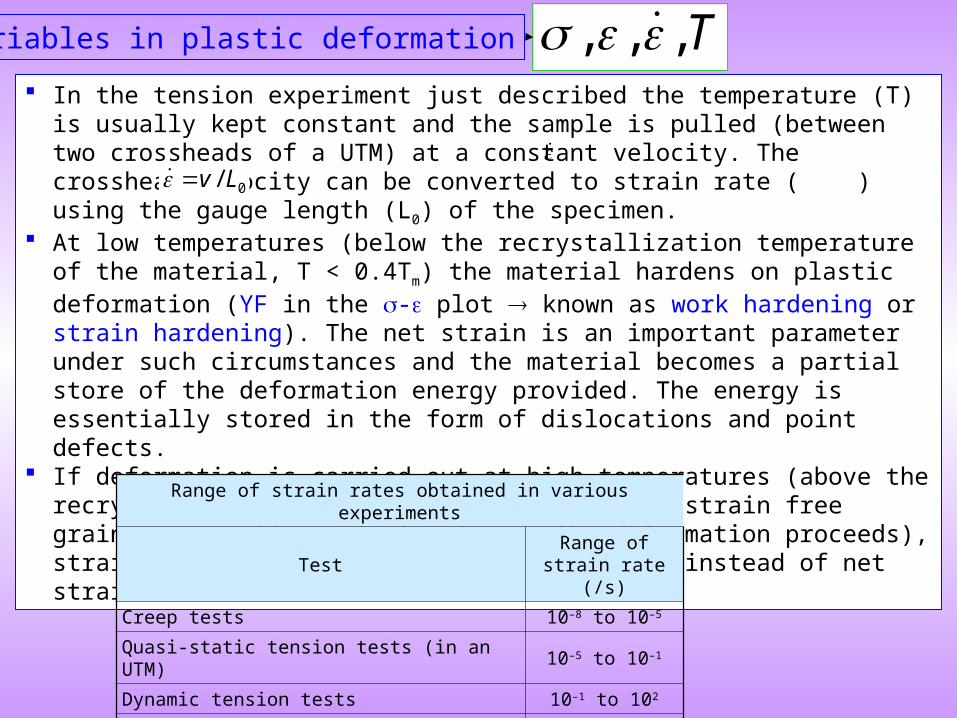
Variables in plastic deformation T , , , In the tension experiment just described the temperature (T) is usually kept constant and

the sample is pulled (between two crossheads of a UTM) at a constant velocity. The crosshead velocity can be converted to strain rate ( ) using the gauge length (L0) of the specimen.

At low temperatures (below the recrystallization temperature of the material, T < 0.4Tm) the material hardens on plastic deformation (YF in the - plot known as work hardening or strain hardening). The net strain is an important parameter under such circumstances and the material becomes a partial store of the deformation energy provided. The energy is essentially stored in the form of dislocations and point defects.

If deformation is carried out at high temperatures (above the recrystallization temperature; wherein, new strain free grains are continuously forming as the deformation proceeds), strain rate becomes the important parameter instead of net strain.

Range of strain rates obtained in various experiments

TestRange of strain

rate (/s)

Creep tests 10–8 to 10–5

Quasi-static tension tests (in an UTM) 10–5 to 10–1

Dynamic tension tests 10–1 to 102

High strain rate tests using impact bars 102 to 104

Explosive loading using projectiles (shock tests) 104 to 108

0/v L

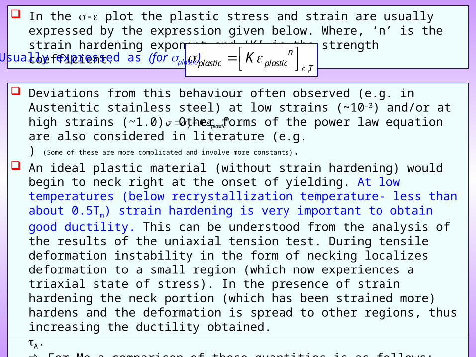
In the - plot the plastic stress and strain are usually expressed by the expression given below. Where, ‘n’ is the strain hardening exponent and ‘K’ is the strength coefficient.

,

nplastic plastic

TK

Usually expressed as (for plastic)

For an experiment done in shear on single crystals the equivalent region to OY can further be subdivided into: True elastic strain (microscopic) till the true elastic limit (E) Onset of microscopic plastic deformation above a stress of A. For Mo a comparison of these quantities is as follows: E = 0.5 MPa, A = 5 MPa and 0 (macroscopic yield stress in shear) = 50 MPa.

Deviations from this behaviour often observed (e.g. in Austenitic stainless steel) at low strains (~10–3) and/or at high strains (~1.0). Other forms of the power law equation are also considered in literature (e.g. ) (Some of these are more complicated and involve more constants).

An ideal plastic material (without strain hardening) would begin to neck right at the onset of yielding. At low temperatures (below recrystallization temperature- less than about 0.5Tm) strain hardening is very important to obtain good ductility. This can be understood from the analysis of the results of the uniaxial tension test. During tensile deformation instability in the form of necking localizes deformation to a small region (which now experiences a triaxial state of stress). In the presence of strain hardening the neck portion (which has been strained more) hardens and the deformation is spread to other regions, thus increasing the ductility obtained.

ny plasticK

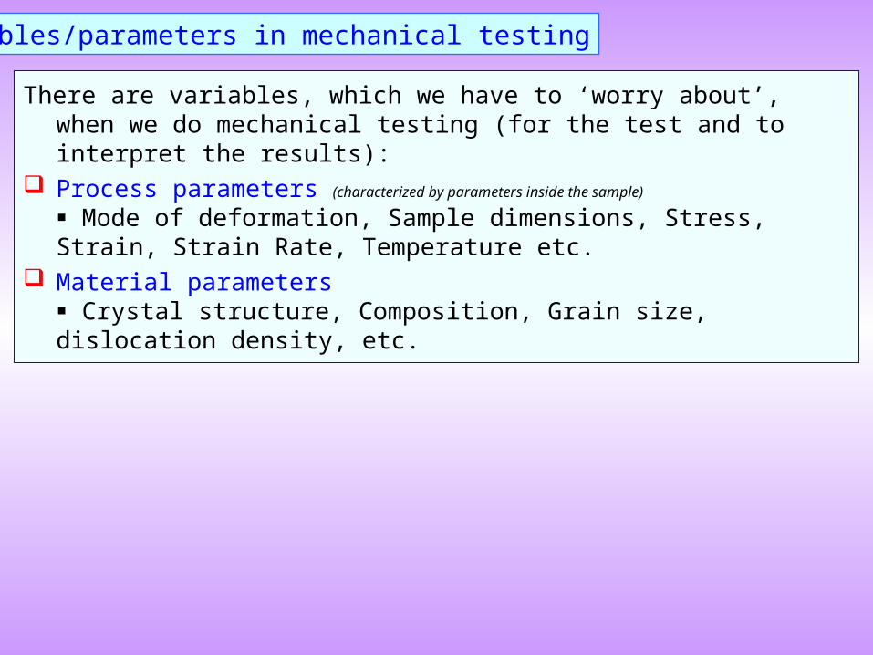
There are variables, which we have to ‘worry about’, when we do mechanical testing (for the test and to interpret the results):

Process parameters (characterized by parameters inside the sample)

Mode of deformation, Sample dimensions, Stress, Strain, Strain Rate, Temperature etc.

Material parameters Crystal structure, Composition, Grain size, dislocation density, etc.

Variables/parameters in mechanical testing

,

n

TK

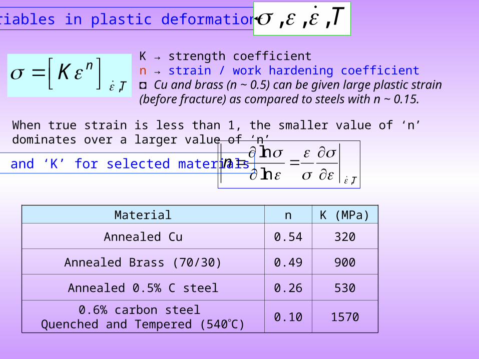
Variables in plastic deformation T , , ,

When true strain is less than 1, the smaller value of ‘n’ dominates over a larger value of ‘n’

K → strength coefficientn → strain / work hardening coefficient◘ Cu and brass (n ~ 0.5) can be given large plastic strain (before fracture) as compared to steels with n ~ 0.15.

Material n K (MPa)

Annealed Cu 0.54 320

Annealed Brass (70/30) 0.49 900

Annealed 0.5% C steel 0.26 530

0.6% carbon steel Quenched and Tempered (540C)

0.10 1570

‘n’ and ‘K’ for selected materials ,

ln

ln T

n

,

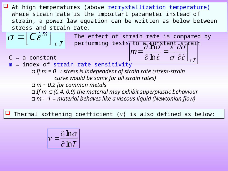
m

TC

C → a constantm → index of strain rate sensitivity

◘ If m = 0 stress is independent of strain rate (stress-strain curve would be same for all strain rates)

◘ m ~ 0.2 for common metals◘ If m (0.4, 0.9) the material may exhibit superplastic behaviour◘ m = 1 → material behaves like a viscous liquid (Newtonian flow)

The effect of strain rate is compared by performing tests to a constant strain

At high temperatures (above recrystallization temperature) where strain rate is the important parameter instead of strain, a power law equation can be written as below between stress and strain rate.

,

ln

ln T

m

Thermal softening coefficient () is also defined as below:

ln

lnT

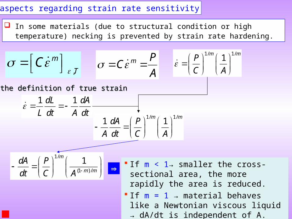
In some materials (due to structural condition or high temperature) necking is prevented by strain rate hardening.

Further aspects regarding strain rate sensitivity

,

m

TC

m P

CA

1/ 1/

1m m

P

C A

From the definition of true strainFrom the definition of true strain

1 1dL dA

L dt A dt

1/ 1/1 1

m mdA P

A dt C A

1/

(1 ) /

1m

m m

dA P

dt C A

If m < 1→ smaller the cross-sectional area, the more rapidly the area is reduced.

If m = 1 → material behaves like a Newtonian viscous liquid → dA/dt is independent of A.

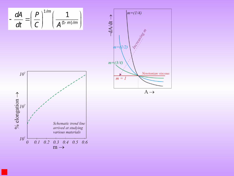
1/

(1 ) /

1m

m m

dA P

dt C A

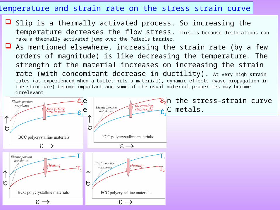
Slip is a thermally activated process. So increasing the temperature decreases the flow stress. This is because dislocations can make a thermally activated jump over the Peierls barrier.

As mentioned elsewhere, increasing the strain rate (by a few orders of magnitude) is like decreasing the temperature. The strength of the material increases on increasing the strain rate (with concomitant decrease in ductility). At very high strain rates (as experienced when a bullet hits a material), dynamic effects (wave propagation in the structure) become important and some of the usual material properties may become irrelevant.

The effect of these two parameters on the stress-strain curve is slightly different for FCC and BCC metals.

Effect of temperature and strain rate on the stress strain curve

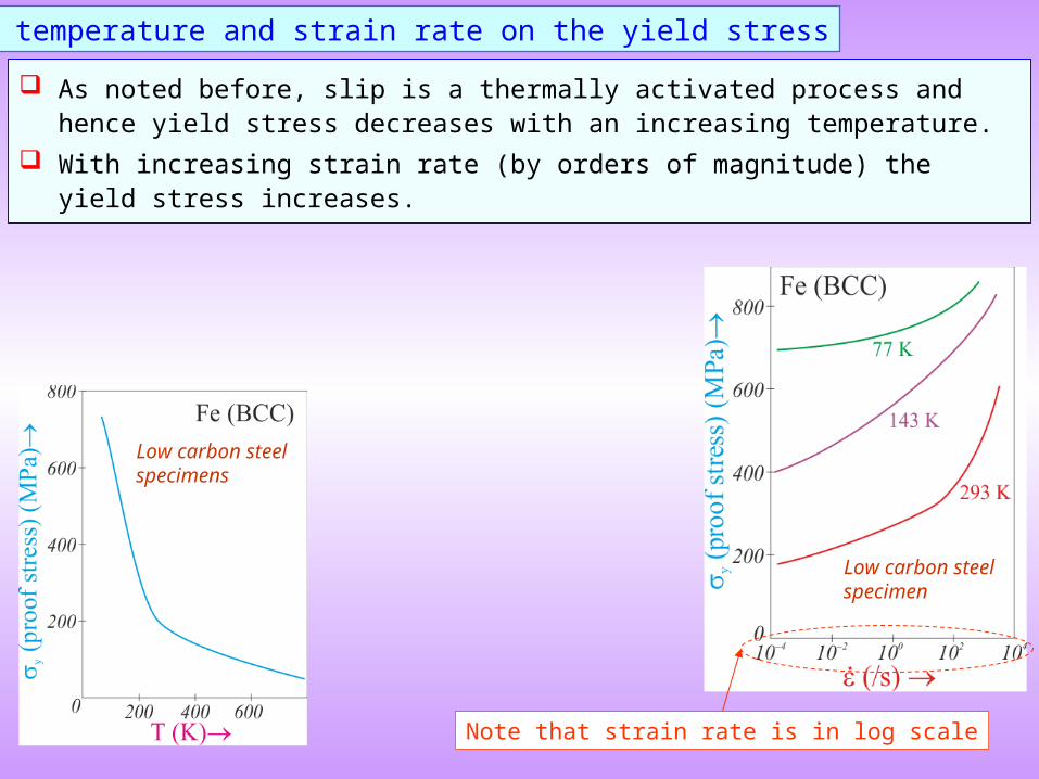
Note that strain rate is in log scale

As noted before, slip is a thermally activated process and hence yield stress decreases with an increasing temperature.

With increasing strain rate (by orders of magnitude) the yield stress increases.

Effect of temperature and strain rate on the yield stress

Low carbon steel specimens

Low carbon steel specimen

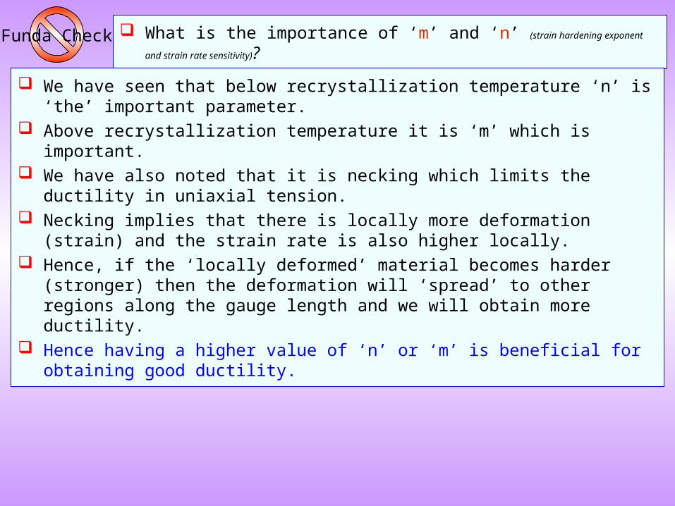
Funda Check What is the importance of ‘m’ and ‘n’ (strain hardening exponent and strain rate sensitivity)?

We have seen that below recrystallization temperature ‘n’ is ‘the’ important parameter. Above recrystallization temperature it is ‘m’ which is important. We have also noted that it is necking which limits the ductility in uniaxial tension. Necking implies that there is locally more deformation (strain) and the strain rate is also

higher locally. Hence, if the ‘locally deformed’ material becomes harder (stronger) then the deformation

will ‘spread’ to other regions along the gauge length and we will obtain more ductility. Hence having a higher value of ‘n’ or ‘m’ is beneficial for obtaining good ductility.

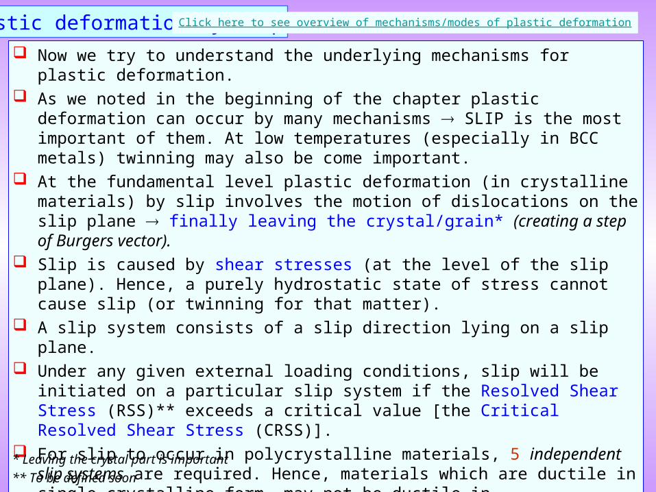
Now we try to understand the underlying mechanisms for plastic deformation. As we noted in the beginning of the chapter plastic deformation can occur by many

mechanisms SLIP is the most important of them. At low temperatures (especially in BCC metals) twinning may also be come important.

At the fundamental level plastic deformation (in crystalline materials) by slip involves the motion of dislocations on the slip plane finally leaving the crystal/grain* (creating a step of Burgers vector).

Slip is caused by shear stresses (at the level of the slip plane). Hence, a purely hydrostatic state of stress cannot cause slip (or twinning for that matter).

A slip system consists of a slip direction lying on a slip plane. Under any given external loading conditions, slip will be initiated on a particular slip

system if the Resolved Shear Stress (RSS)** exceeds a critical value [the Critical Resolved Shear Stress (CRSS)].

For slip to occur in polycrystalline materials, 5 independent slip systems are required. Hence, materials which are ductile in single crystalline form, may not be ductile in polycrystalline form. CCP crystals (Cu, Al, Au) have excellent ductility.

At higher temperatures more slip systems may become active and hence polycrystalline materials which are brittle at low temperature, may become ductile at high temperature.

Plastic deformation by slip Click here to see overview of mechanisms/modes of plastic deformation

* Leaving the crystal part is important

** To be defined soon

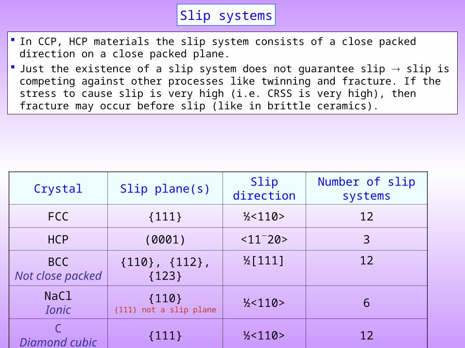
Crystal Slip plane(s) Slip direction Number of slip systems

FCC {111} ½<110> 12

HCP (0001) <1120> 3

BCCNot close packed

{110}, {112}, {123}½[111] 12

NaClIonic

{110}{111} not a slip plane

½<110> 6

CDiamond cubic

{111} ½<110> 12

Slip systems

In CCP, HCP materials the slip system consists of a close packed direction on a close packed plane. Just the existence of a slip system does not guarantee slip slip is competing against other processes

like twinning and fracture. If the stress to cause slip is very high (i.e. CRSS is very high), then fracture may occur before slip (like in brittle ceramics).

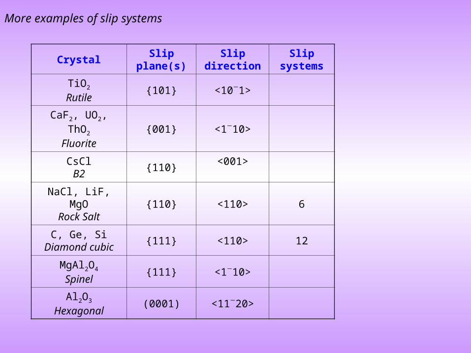
Crystal Slip plane(s) Slip direction Slip systems

TiO2

Rutile{101} <101>

CaF2, UO2, ThO2

Fluorite{001} <110>

CsClB2

{110}<001>

NaCl, LiF, MgORock Salt

{110} <110> 6

C, Ge, SiDiamond cubic

{111} <110> 12

MgAl2O4

Spinel{111} <110>

Al2O3

Hexagonal(0001) <1120>

More examples of slip systems

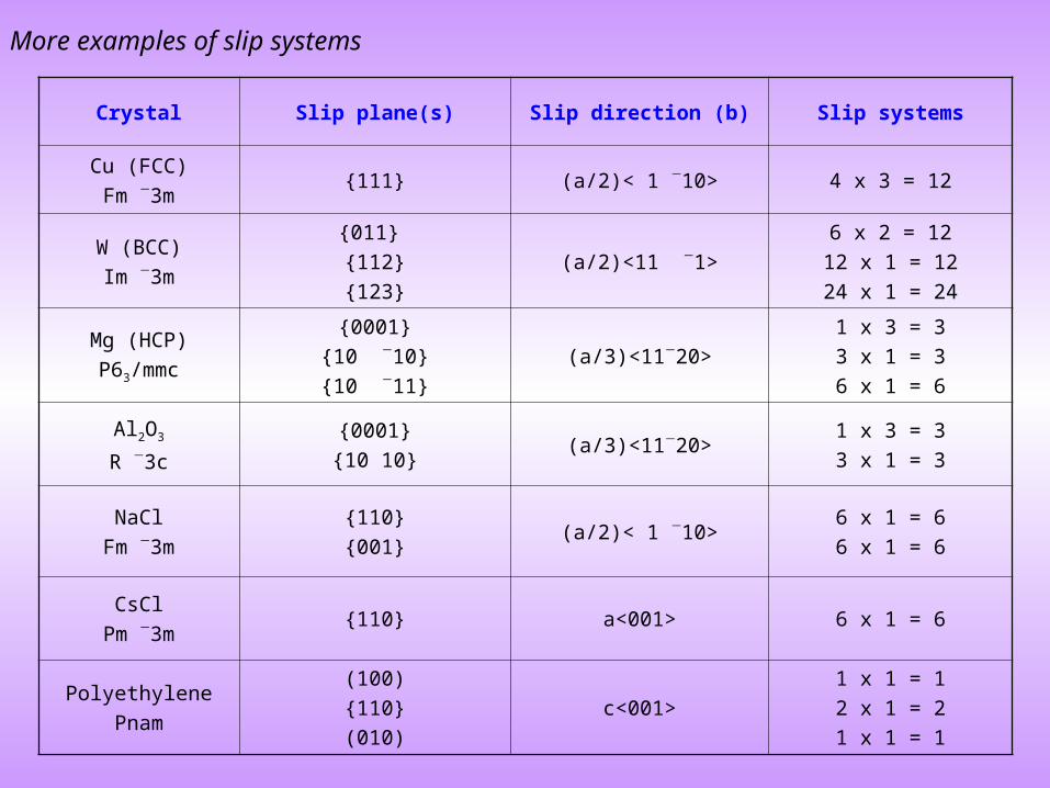
Crystal Slip plane(s) Slip direction (b) Slip systems

Cu (FCC)

Fm 3m{111} (a/2)< 1 10> 4 x 3 = 12

W (BCC)

Im 3m

{011}

{112}

{123}

(a/2)<11 1>

6 x 2 = 12

12 x 1 = 12

24 x 1 = 24

Mg (HCP)

P63/mmc

{0001}

{10 10}

{10 11}

(a/3)<1120>

1 x 3 = 3

3 x 1 = 3

6 x 1 = 6

Al2O3

R 3c

{0001}

{10 10}(a/3)<1120>

1 x 3 = 3

3 x 1 = 3

NaCl

Fm 3m

{110}

{001}(a/2)< 1 10>

6 x 1 = 6

6 x 1 = 6

CsCl

Pm 3m{110} a<001> 6 x 1 = 6

Polyethylene

Pnam

(100)

{110}

(010)

c<001>

1 x 1 = 1

2 x 1 = 2

1 x 1 = 1

More examples of slip systems

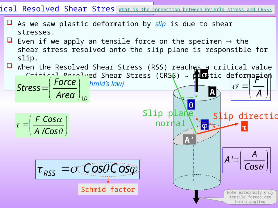
As we saw plastic deformation by slip is due to shear stresses. Even if we apply an tensile force on the specimen the shear stress resolved onto the slip

plane is responsible for slip. When the Resolved Shear Stress (RSS) reaches a critical value → Critical Resolved Shear

Stress (CRSS) → plastic deformation starts (The actual Schmid’s law)

Slip plane normal

Slip direction

A’

DArea

ForceStress

1

CosA

CosF

/

RSS Cos Cos

A

Cos

AA'

A

F

Schmid factor

Critical Resolved Shear Stress (CRSS)

Note externally only tensile forces are being applied

What is the connection between Peierls stress and CRSS?

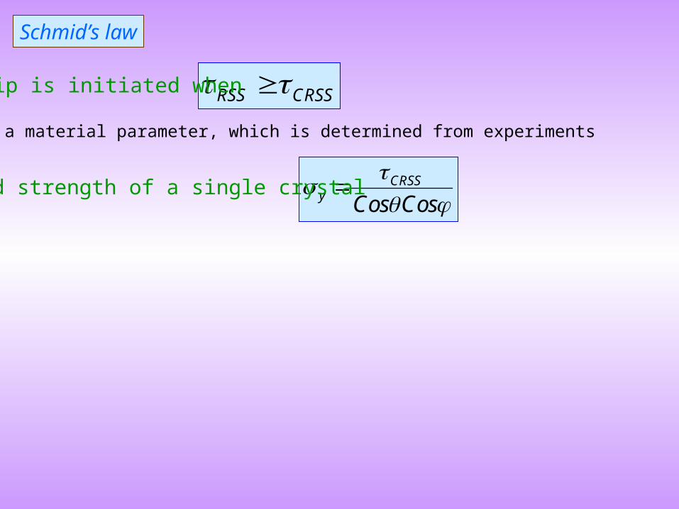
Schmid’s law

CRSSy Cos Cos

RSS CRSS Slip is initiated when

Yield strength of a single crystal

CRSS is a material parameter, which is determined from experiments

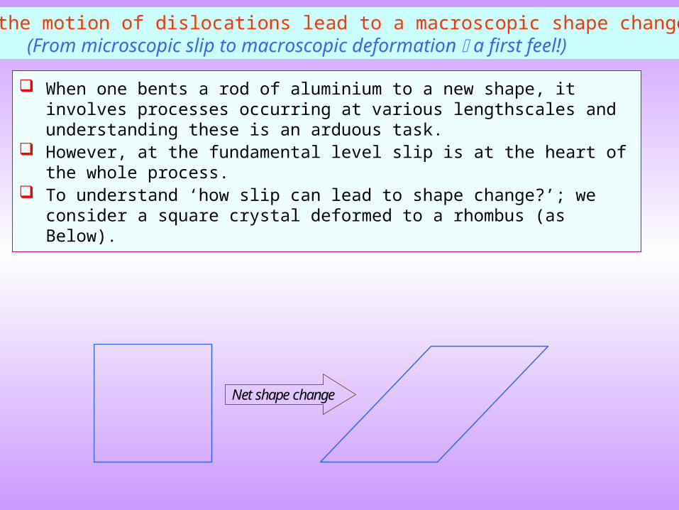
How does the motion of dislocations lead to a macroscopic shape change?(From microscopic slip to macroscopic deformation a first feel!)

Net shape change

When one bents a rod of aluminium to a new shape, it involves processes occurring at various lengthscales and understanding these is an arduous task.

However, at the fundamental level slip is at the heart of the whole process. To understand ‘how slip can lead to shape change?’; we consider a square crystal

deformed to a rhombus (as Below).

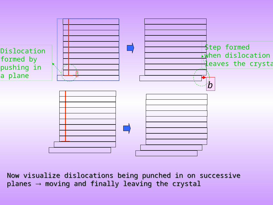
b

Dislocation formed bypushing ina plane

Step formed when dislocationleaves the crystal

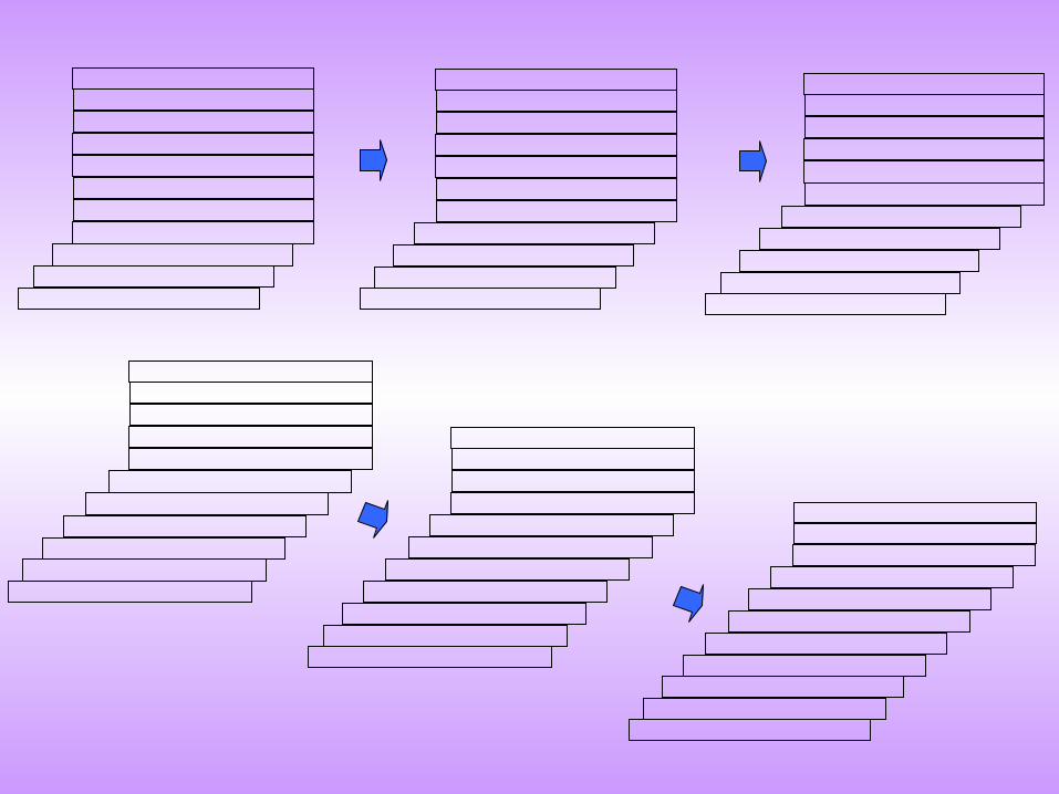
Now visualize dislocations being punched in on successive planes moving and finally leaving the crystalNow visualize dislocations being punched in on successive planes moving and finally leaving the crystal

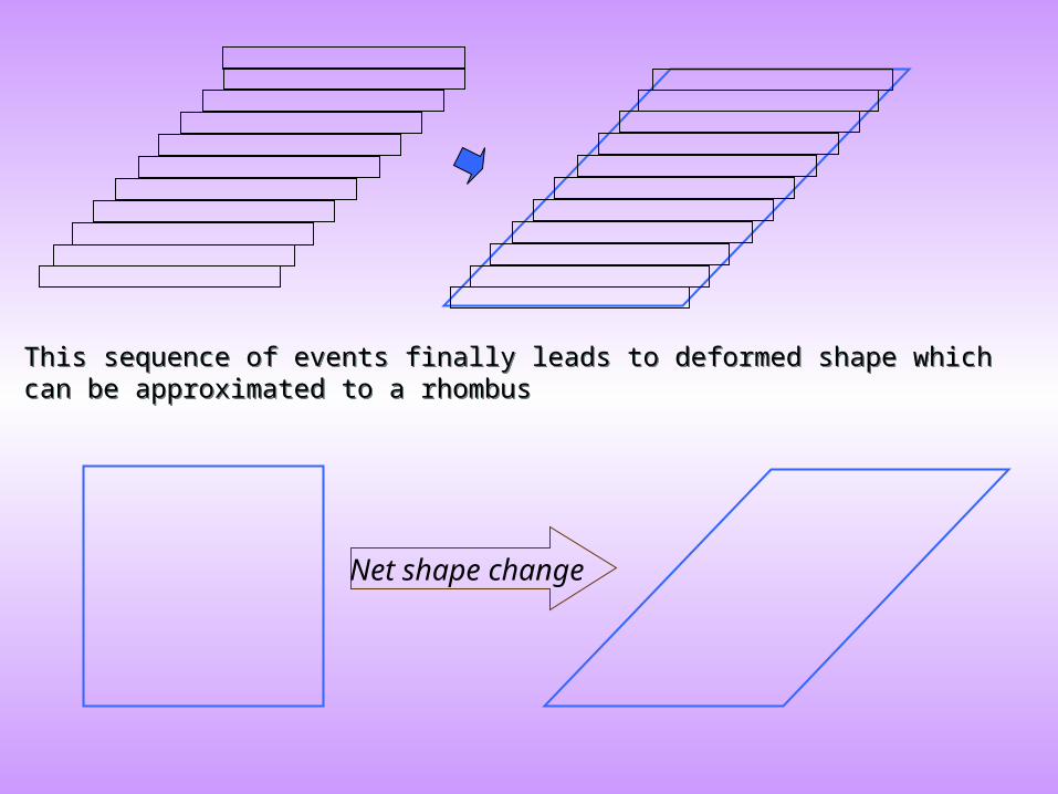
Net shape change

This sequence of events finally leads to deformed shape which can be approximated to a rhombusThis sequence of events finally leads to deformed shape which can be approximated to a rhombus

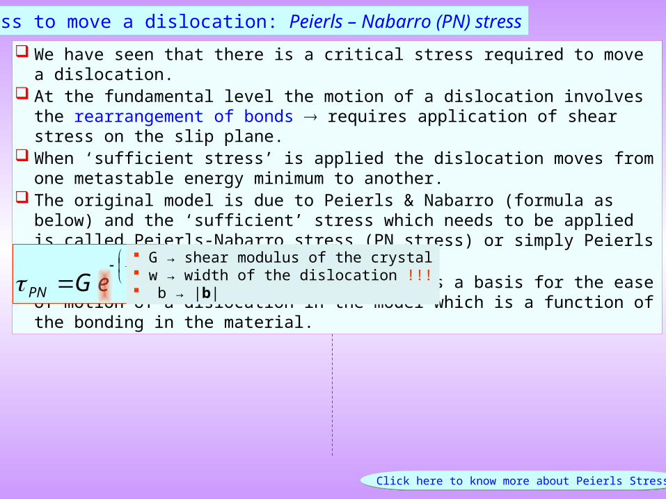
Stress to move a dislocation: Peierls – Nabarro (PN) stress

We have seen that there is a critical stress required to move a dislocation. At the fundamental level the motion of a dislocation involves the rearrangement of bonds

requires application of shear stress on the slip plane. When ‘sufficient stress’ is applied the dislocation moves from one metastable energy

minimum to another. The original model is due to Peierls & Nabarro (formula as below) and the ‘sufficient’ stress

which needs to be applied is called Peierls-Nabarro stress (PN stress) or simply Peierls stress. Width of the dislocation is considered as a basis for the ease of motion of a dislocation in the

model which is a function of the bonding in the material.

Click here to know more about Peierls StressClick here to know more about Peierls Stress

b

w

PN eG

2

G → shear modulus of the crystal w → width of the dislocation !!! b → |b|

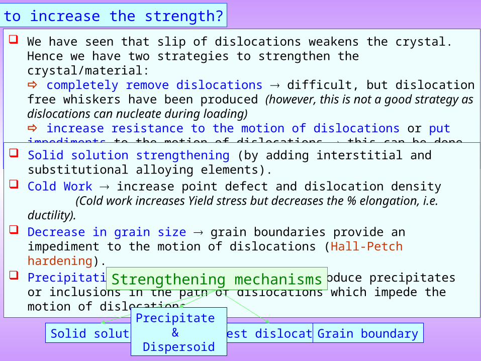
How to increase the strength?

We have seen that slip of dislocations weakens the crystal. Hence we have two strategies to strengthen the crystal/material: completely remove dislocations difficult, but dislocation free whiskers have been produced (however, this is not a good strategy as dislocations can nucleate during loading) increase resistance to the motion of dislocations or put impediments to the motion of dislocations this can be done in many ways as listed below.

Solid solution strengthening (by adding interstitial and substitutional alloying elements). Cold Work increase point defect and dislocation density

(Cold work increases Yield stress but decreases the % elongation, i.e. ductility). Decrease in grain size grain boundaries provide an impediment to the motion of

dislocations (Hall-Petch hardening). Precipitation/dispersion hardening introduce precipitates or inclusions in the path of

dislocations which impede the motion of dislocations.

Forest dislocation

Strengthening mechanisms

Solid solutionPrecipitate

& Dispersoid

Grain boundary

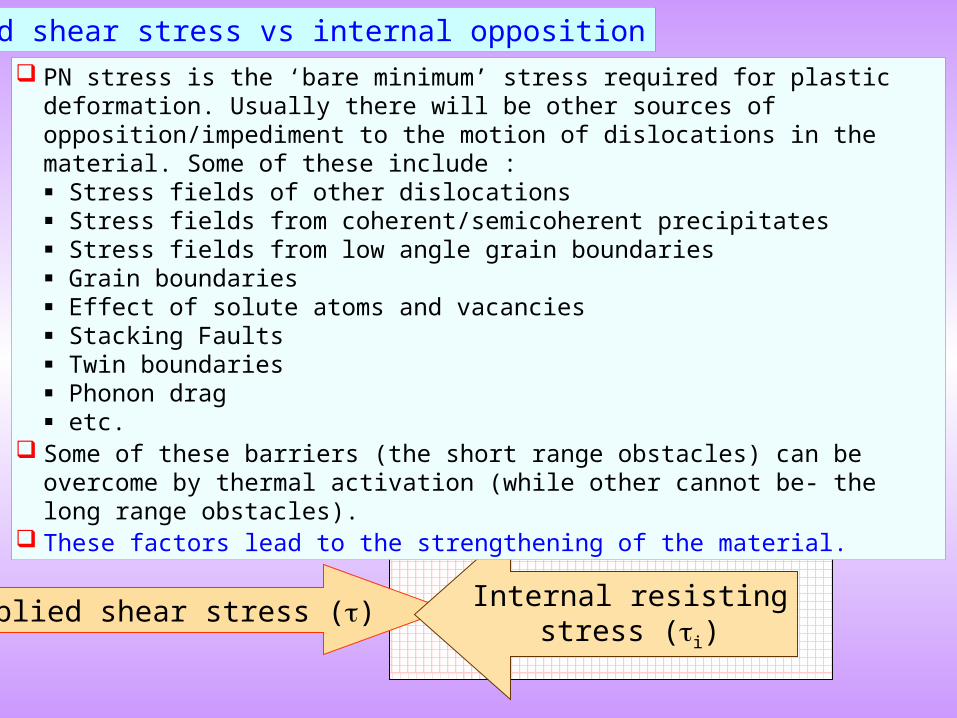
Applied shear stress vs internal opposition

Applied shear stress () Internal resisting stress (i)

PN stress is the ‘bare minimum’ stress required for plastic deformation. Usually there will be other sources of opposition/impediment to the motion of dislocations in the material. Some of these include : Stress fields of other dislocations Stress fields from coherent/semicoherent precipitates Stress fields from low angle grain boundaries Grain boundaries Effect of solute atoms and vacancies Stacking Faults Twin boundaries Phonon drag etc.

Some of these barriers (the short range obstacles) can be overcome by thermal activation (while other cannot be- the long range obstacles).

These factors lead to the strengthening of the material.

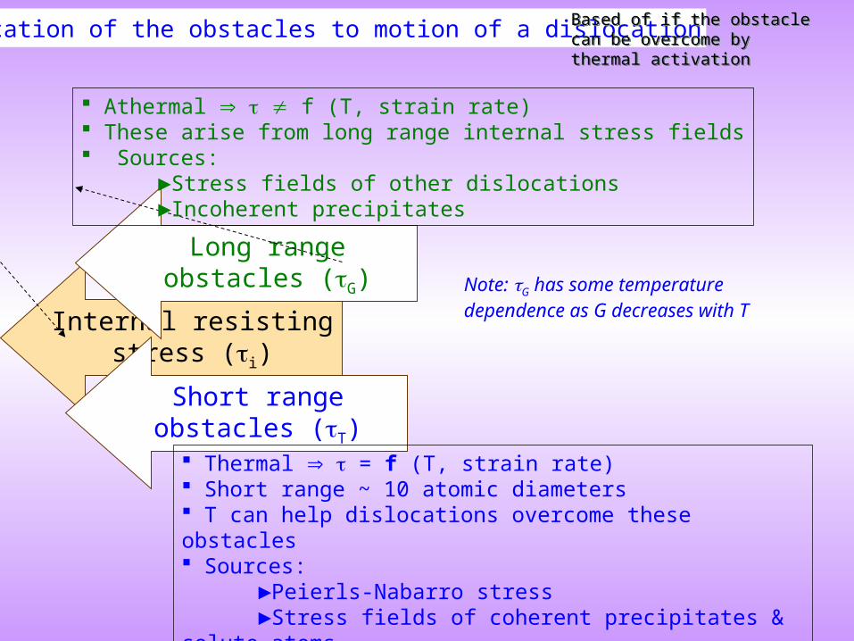
Internal resisting stress (i)

Long range obstacles (G)

Short range obstacles (T)

Athermal f (T, strain rate) These arise from long range internal stress fields Sources: ►Stress fields of other dislocations ►Incoherent precipitates

Note: G has some temperature dependence as G decreases with T

Thermal = f (T, strain rate) Short range ~ 10 atomic diameters T can help dislocations overcome these obstacles Sources: ►Peierls-Nabarro stress ►Stress fields of coherent precipitates & solute atoms

Classification of the obstacles to motion of a dislocation Based of if the obstacle can be overcome by thermal activationBased of if the obstacle can be overcome by thermal activation

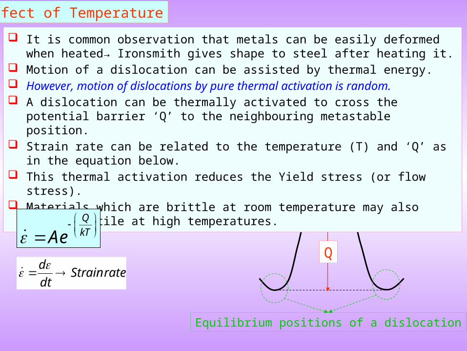
Effect of Temperature

Equilibrium positions of a dislocation

Q

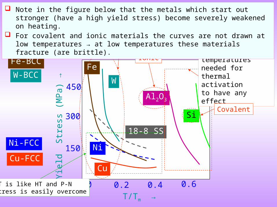
It is common observation that metals can be easily deformed when heated→ Ironsmith gives shape to steel after heating it.

Motion of a dislocation can be assisted by thermal energy. However, motion of dislocations by pure thermal activation is random. A dislocation can be thermally activated to cross the potential barrier ‘Q’ to the

neighbouring metastable position. Strain rate can be related to the temperature (T) and ‘Q’ as in the equation below. This thermal activation reduces the Yield stress (or flow stress). Materials which are brittle at room temperature may also become ductile at high

temperatures.

Q

kTAe

rateStraindt

d

Fe

W

18-8 SS

Cu

Ni

Al2O3

Si

150

300

450

0.2 0.4 0.60.0

Yie

ld S

tres

s (M

Pa)

→

T/Tm →

Very high temperaturesneeded for thermal activationto have any effect

RT is like HT and P-Nstress is easily overcome

Fe-BCC

W-BCC

Cu-FCC

Ni-FCC

Metallic

Ionic

Covalent

Note in the figure below that the metals which start out stronger (have a high yield stress) become severely weakened on heating.

For covalent and ionic materials the curves are not drawn at low temperatures → at low temperatures these materials fracture (are brittle).

What causes Strain hardening? → multiplication of dislocations

Hence two important questions need to be answered: How does the dislocation density increase? What leads to strain hardening?

6 9 12 14

dislocation dislocation

~ (10 10 ) ~ (10 10 )Cold workAnnealed material Stronger material

Strain hardening

→

X

Strain hardening →

→

→

X

Strain hardening →

→

The increase in flow stress with strain is called strain hardening (or work hardening).

Plastic deformation is caused by dislocations moving and leaving the crystal that dislocation density should decrease with plastic deformation. However, it is observed that dislocation density increases with strain! Further, if dislocations are the agent weakening the crystal then with increased dislocation density the material should get weaker! But, we observe on the contrary an increase in strength!

This implies some sources of dislocation multiplication / creation should exist &

More dislocations is somehow causing a ‘traffic jam’ kind of scenario and leading to strengthening.

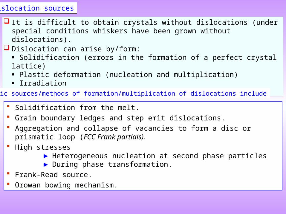
Dislocation sources

Solidification from the melt. Grain boundary ledges and step emit dislocations. Aggregation and collapse of vacancies to form a disc or prismatic loop (FCC Frank

partials). High stresses

► Heterogeneous nucleation at second phase particles► During phase transformation.

Frank-Read source. Orowan bowing mechanism.

It is difficult to obtain crystals without dislocations (under special conditions whiskers have been grown without dislocations).

Dislocation can arise by/form: Solidification (errors in the formation of a perfect crystal lattice) Plastic deformation (nucleation and multiplication) Irradiation etc.

Some specific sources/methods of formation/multiplication of dislocations include

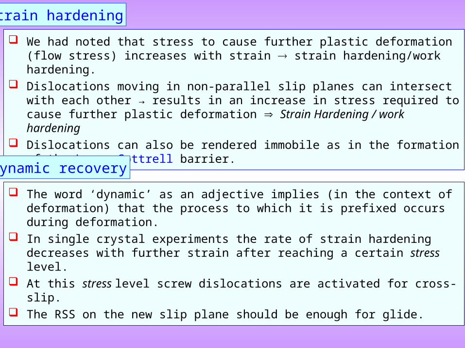
Strain hardening

We had noted that stress to cause further plastic deformation (flow stress) increases with strain strain hardening/work hardening.

Dislocations moving in non-parallel slip planes can intersect with each other → results in an increase in stress required to cause further plastic deformation Strain Hardening / work hardening

Dislocations can also be rendered immobile as in the formation of the Lomer-Cottrell barrier.

Dynamic recovery

The word ‘dynamic’ as an adjective implies (in the context of deformation) that the process to which it is prefixed occurs during deformation.

In single crystal experiments the rate of strain hardening decreases with further strain after reaching a certain stress level.

At this stress level screw dislocations are activated for cross-slip. The RSS on the new slip plane should be enough for glide.

)111(

]1 0 1[2

1

)111(

]0 1 1[2

1

)100(

]1 1 0[2

1

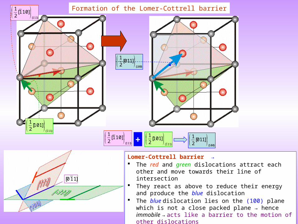
Formation of the Lomer-Cottrell barrier

]1 1 0[

)100(

]1 1 0[2

1

)111(

]0 1 1[2

1

)111(

]1 0 1[2

1

+

Lomer-Cottrell barrier → The red and green dislocations attract each other and move

towards their line of intersection They react as above to reduce their energy and produce the blue

dislocation The blue dislocation lies on the (100) plane which is not a close

packed plane → hence immobile → acts like a barrier to the motion of other dislocations

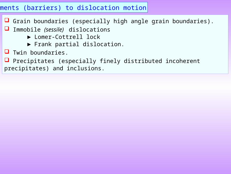
Impediments (barriers) to dislocation motion

Grain boundaries (especially high angle grain boundaries). Immobile (sessile) dislocations

► Lomer-Cottrell lock► Frank partial dislocation.

Twin boundaries. Precipitates (especially finely distributed incoherent precipitates) and inclusions.

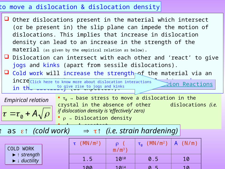
Stress to move a dislocation & dislocation density

A 0

0 → base stress to move a dislocation in the crystal in the absence of other dislocations (i.e. if dislocation density is ‘effectively’ zero) → Dislocation density A → A constant

↑ as ↑ (cold work) ↑ (i.e. strain hardening)

Empirical relation

(MN/m2) ( m/m3) 0 (MN/m2) A (N/m)

1.5 1010 0.5 10

100 1014 0.5 10

COLD WORK ► ↑ strength ► ↓ ductility

COLD WORK ► ↑ strength ► ↓ ductility

Other dislocations present in the material which intersect (or be present in) the slip plane can impede the motion of dislocations. This implies that increase in dislocation density can lead to an increase in the strength of the material (as given by the empirical relation as below).

Dislocation can intersect with each other and ‘react’ to give jogs and kinks (apart from sessile dislocations).

Cold work will increase the strength of the material via an increase in dislocation density, but will lead to a decrease in the ductility (as expected!).

Dislocation ReactionsDislocation ReactionsClick here to know more about dislocation interactionsto give rise to jogs and kinks

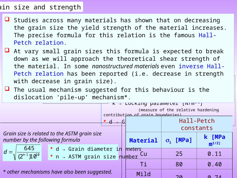
Grain size and strength

d

kiy

y → Yield stress [N/m2]

i → Stress to move a dislocation in single crystal [N/m2]

k → Locking parameter [N/m3/2] (measure of the relative hardening contribution of grain boundaries)

d → Grain diameter [m]

Hall-Petch Relation

Hall-Petch constants

Material i [MPa] k [MPa m1/2]

Cu 25 0.11

Ti 80 0.40

Mild steel 70 0.74

Ni3Al 300 1.70

101 10)2(

645

nd

d → Grain diameter in meters n → ASTM grain size number

Grain size is related to the ASTM grain size number by the following formula

Studies across many materials has shown that on decreasing the grain size the yield strength of the material increases. The precise formula for this relation is the famous Hall-Petch relation.

At vary small grain sizes this formula is expected to break down as we will approach the theoretical shear strength of the material. In some nanostructured materials even inverse Hall-Petch relation has been reported (i.e. decrease in strength with decrease in grain size).

The usual mechanism suggested for this behaviour is the dislocation ‘pile-up’ mechanism*.

* other mechanisms have also been suggested.

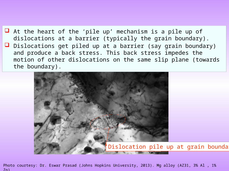
Photo courtesy: Dr. Eswar Prasad (Johns Hopkins University, 2013). Mg alloy (AZ31, 3% Al , 1% Zn)

At the heart of the ‘pile up’ mechanism is a pile up of dislocations at a barrier (typically the grain boundary).

Dislocations get piled up at a barrier (say grain boundary) and produce a back stress. This back stress impedes the motion of other dislocations on the same slip plane (towards the boundary).

Dislocation pile up at grain boundary

Effect of solute atoms on strengthening

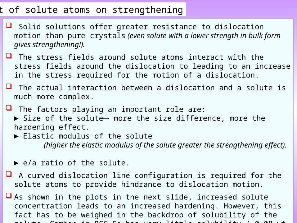
Solid solutions offer greater resistance to dislocation motion than pure crystals (even solute with a lower strength in bulk form gives strengthening!).

The stress fields around solute atoms interact with the stress fields around the dislocation to leading to an increase in the stress required for the motion of a dislocation.

The actual interaction between a dislocation and a solute is much more complex.

The factors playing an important role are:► Size of the solute more the size difference, more the hardening effect.► Elastic modulus of the solute

(higher the elastic modulus of the solute greater the strengthening effect). ► e/a ratio of the solute.

A curved dislocation line configuration is required for the solute atoms to provide hindrance to dislocation motion.

As shown in the plots in the next slide, increased solute concentration leads to an increased hardening. However, this fact has to be weighed in the backdrop of solubility of the solute. Carbon in BCC Fe has very little solubility (~0.08 wt.%) and hence the approach of pure solid solution strengthening to harden a material can have a limited scope.

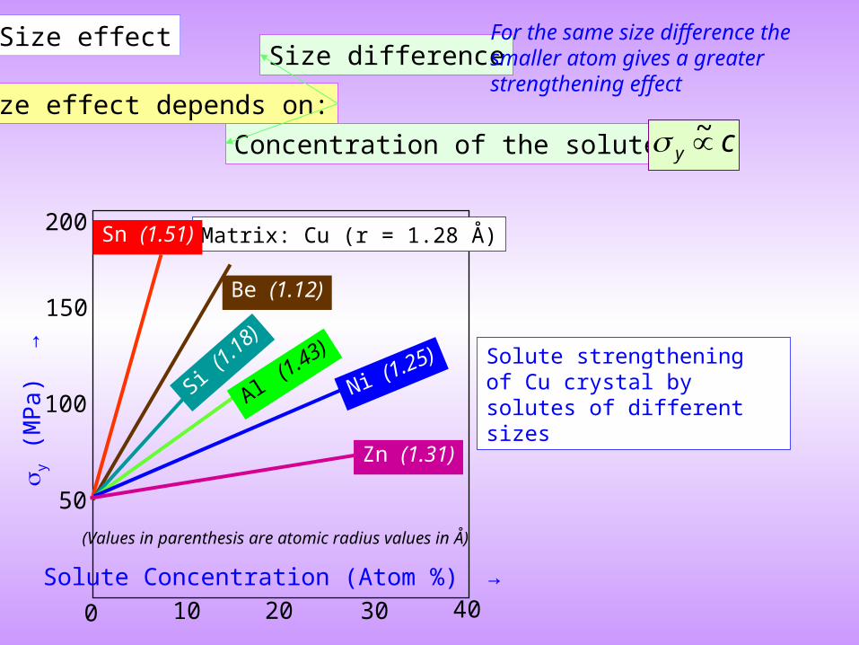
Solute Concentration (Atom %) →

y (M

Pa)

→

50

100

150

10 20 30 40

200

0

Solute strengthening of Cu crystal by solutes of different sizes

Matrix: Cu (r = 1.28 Å)

Be (1.12)

Si (1.18)

Sn (1.51)

Ni (1.25)

Zn (1.31)

Al (1.43)

(Values in parenthesis are atomic radius values in Å)

Size effectSize difference

Size effect depends on:

Concentration of the solute (c) cy ~

For the same size difference thesmaller atom gives a greaterstrengthening effect

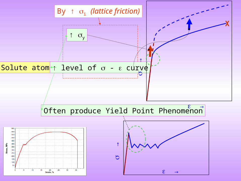
↑ y

Often produce Yield Point Phenomenon

Solute atoms ↑ level of - curve

→

X

→

→

→

By ↑ i (lattice friction)

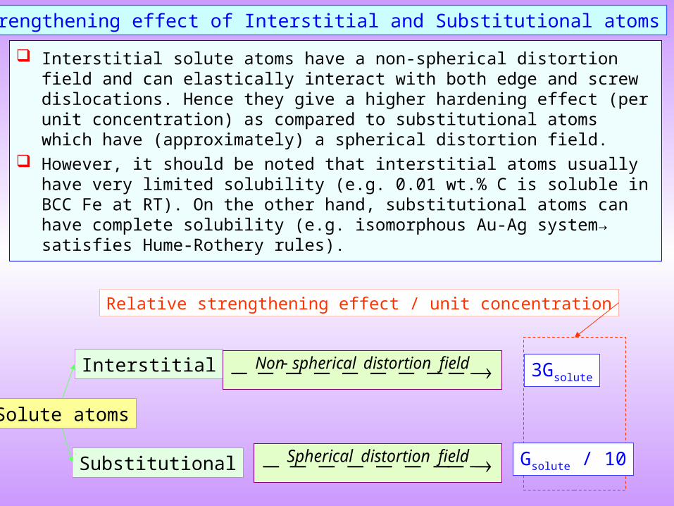
Interstitial

Solute atoms

Substitutional

3Gsolute

Relative strengthening effect / unit concentration

Gsolute / 10 fielddistortionSpherical

fielddistortionsphericalNon

Interstitial solute atoms have a non-spherical distortion field and can elastically interact with both edge and screw dislocations. Hence they give a higher hardening effect (per unit concentration) as compared to substitutional atoms which have (approximately) a spherical distortion field.

However, it should be noted that interstitial atoms usually have very limited solubility (e.g. 0.01 wt.% C is soluble in BCC Fe at RT). On the other hand, substitutional atoms can have complete solubility (e.g. isomorphous Au-Ag system→ satisfies Hume-Rothery rules).

Relative strengthening effect of Interstitial and Substitutional atoms

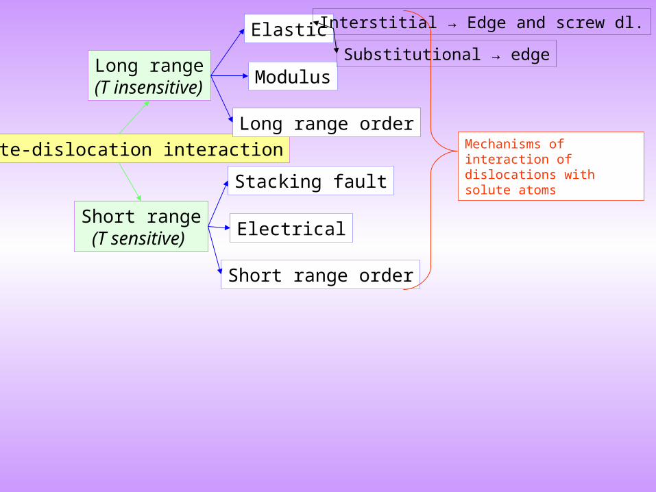
Long range(T insensitive)

Solute-dislocation interaction

Short range (T sensitive)

Modulus

Long range order

ElasticSubstitutional → edge

Interstitial → Edge and screw dl.

Electrical

Short range order

Stacking fault

Mechanisms of interaction of dislocations with solute atoms

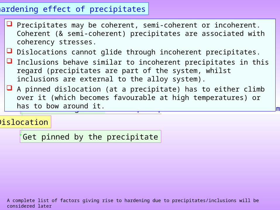
The hardening effect of precipitates

Glide through the precipitate

Dislocation

Get pinned by the precipitate

If the precipitate is coherent with the matrix

Precipitates may be coherent, semi-coherent or incoherent. Coherent (& semi-coherent) precipitates are associated with coherency stresses.

Dislocations cannot glide through incoherent precipitates. Inclusions behave similar to incoherent precipitates in this regard (precipitates are part of

the system, whilst inclusions are external to the alloy system). A pinned dislocation (at a precipitate) has to either climb over it (which becomes

favourable at high temperatures) or has to bow around it.

A complete list of factors giving rise to hardening due to precipitates/inclusions will be considered later

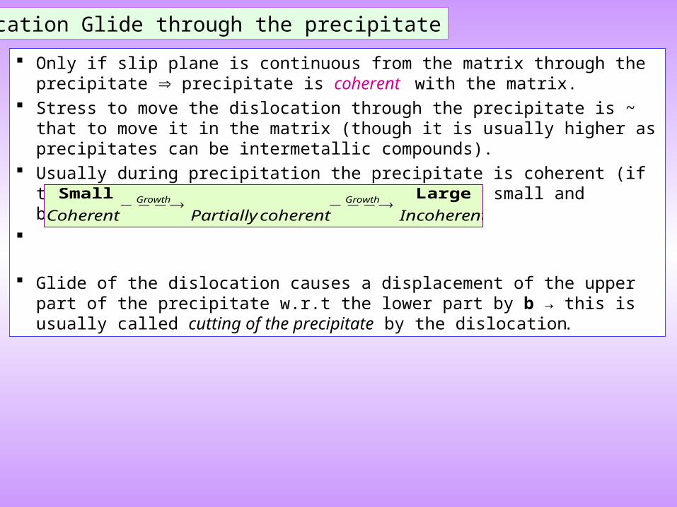
Dislocation Glide through the precipitate

Only if slip plane is continuous from the matrix through the precipitate precipitate is coherent with the matrix.

Stress to move the dislocation through the precipitate is ~ that to move it in the matrix (though it is usually higher as precipitates can be intermetallic compounds).

Usually during precipitation the precipitate is coherent (if the lattice misfit is small) only when it is small and becomes incoherent on growth.

Glide of the dislocation causes a displacement of the upper part of the precipitate w.r.t the lower part by b → this is usually called cutting of the precipitate by the dislocation.

IncoherentcoherentPartially CoherentGrowthGrowth LargeSmall

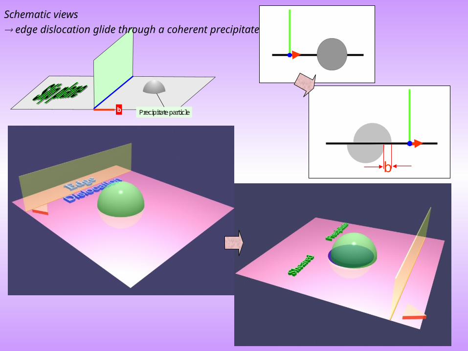
b

Precipitate particleb

Schematic views

edge dislocation glide through a coherent precipitate

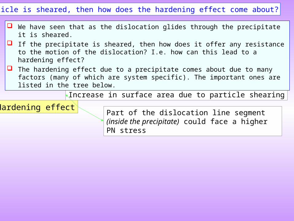
Hardening effectPart of the dislocation line segment (inside the precipitate) could face a higher PN stress

Increase in surface area due to particle shearing

We have seen that as the dislocation glides through the precipitate it is sheared. If the precipitate is sheared, then how does it offer any resistance to the motion of the dislocation? I.e.

how can this lead to a hardening effect? The hardening effect due to a precipitate comes about due to many factors (many of which are system

specific). The important ones are listed in the tree below.

If the particle is sheared, then how does the hardening effect come about?

Pinning effect of inclusions

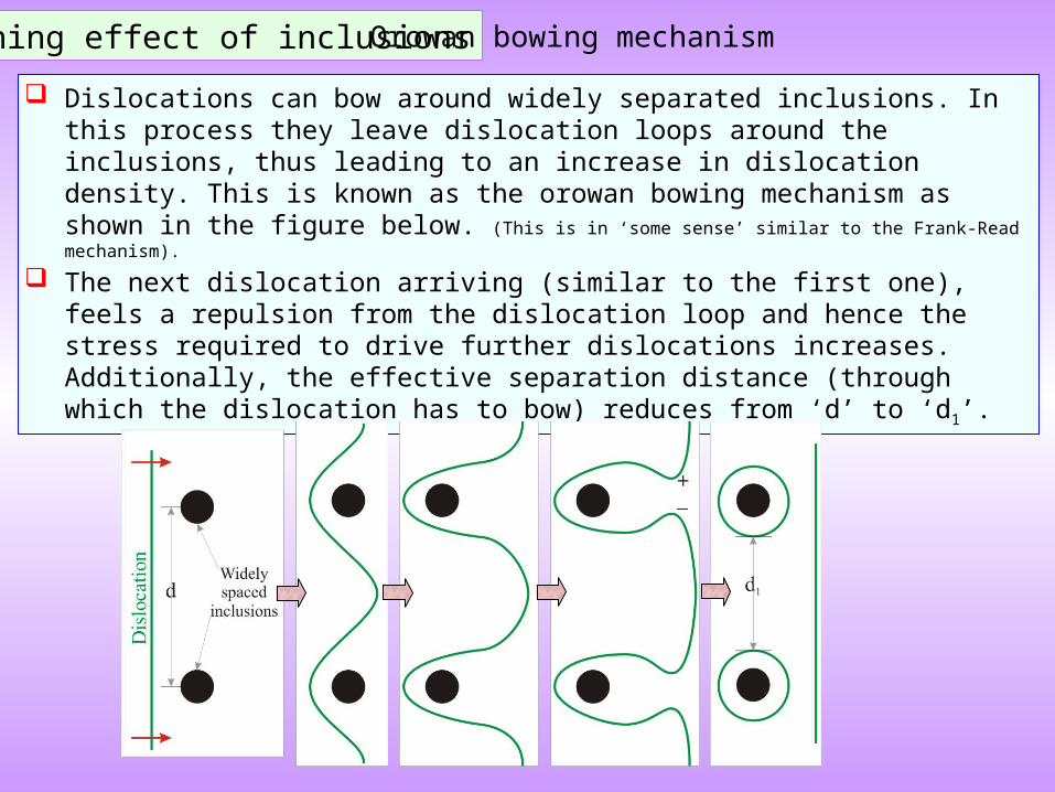
Dislocations can bow around widely separated inclusions. In this process they leave dislocation loops around the inclusions, thus leading to an increase in dislocation density. This is known as the orowan bowing mechanism as shown in the figure below. (This is in ‘some sense’ similar to the Frank-Read mechanism).

The next dislocation arriving (similar to the first one), feels a repulsion from the dislocation loop and hence the stress required to drive further dislocations increases. Additionally, the effective separation distance (through which the dislocation has to bow) reduces from ‘d’ to ‘d1’.

Orowan bowing mechanism

Precipitate Hardening effect

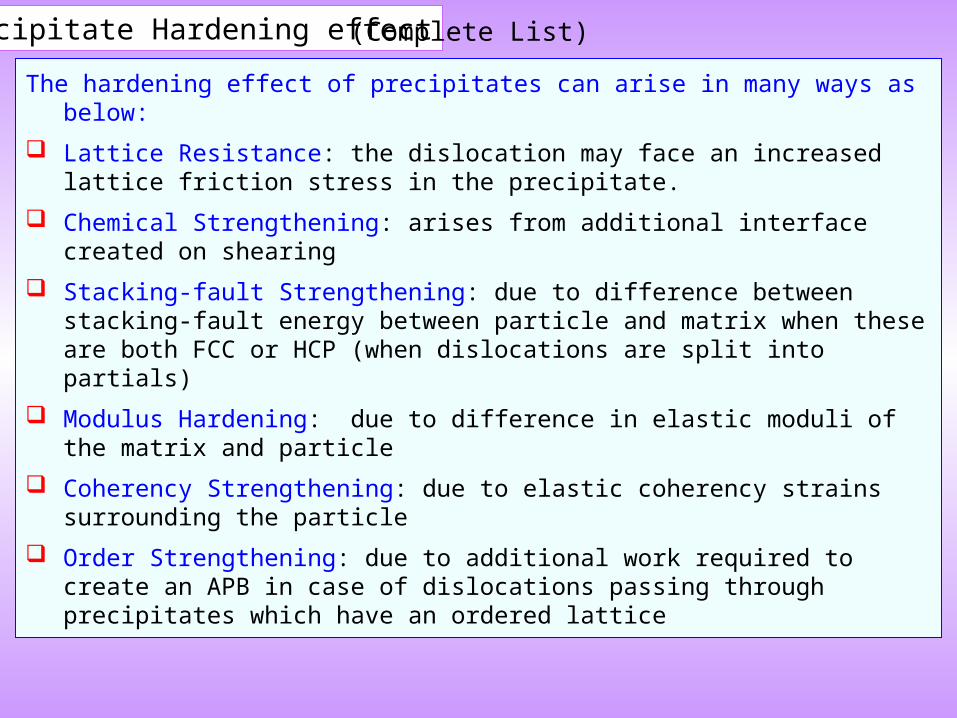
The hardening effect of precipitates can arise in many ways as below:

Lattice Resistance: the dislocation may face an increased lattice friction stress in the precipitate.

Chemical Strengthening: arises from additional interface created on shearing

Stacking-fault Strengthening: due to difference between stacking-fault energy between particle and matrix when these are both FCC or HCP (when dislocations are split into partials)

Modulus Hardening: due to difference in elastic moduli of the matrix and particle

Coherency Strengthening: due to elastic coherency strains surrounding the particle

Order Strengthening: due to additional work required to create an APB in case of dislocations passing through precipitates which have an ordered lattice

(Complete List)

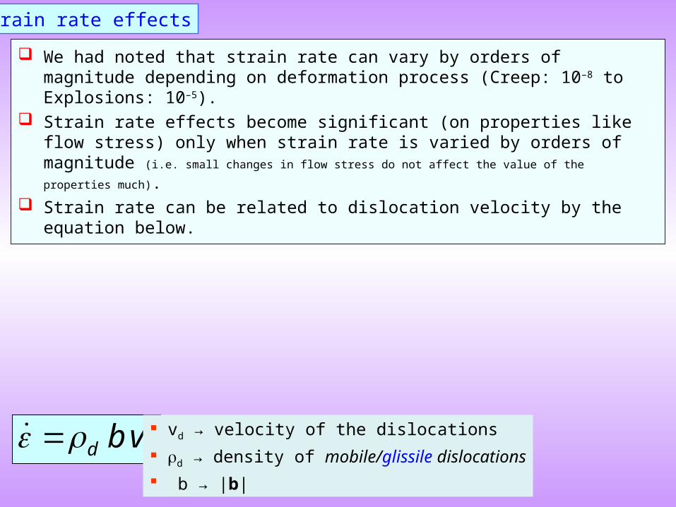
We had noted that strain rate can vary by orders of magnitude depending on deformation process (Creep: 10–8 to Explosions: 10–5).

Strain rate effects become significant (on properties like flow stress) only when strain rate is varied by orders of magnitude (i.e. small changes in flow stress do not affect the value of the properties much).

Strain rate can be related to dislocation velocity by the equation below.

Strain rate effects

dd vb vd → velocity of the dislocations

d → density of mobile/glissile dislocations

b → |b|

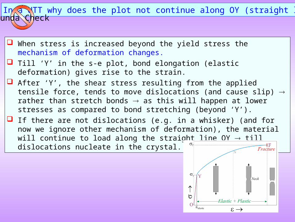
When stress is increased beyond the yield stress the mechanism of deformation changes. Till ‘Y’ in the s-e plot, bond elongation (elastic deformation) gives rise to the strain. After ‘Y’, the shear stress resulting from the applied tensile force, tends to move

dislocations (and cause slip) rather than stretch bonds as this will happen at lower stresses as compared to bond stretching (beyond ‘Y’).

If there are not dislocations (e.g. in a whisker) (and for now we ignore other mechanism of deformation), the material will continue to load along the straight line OY till dislocations nucleate in the crystal.

In a UTT why does the plot not continue along OY (straight line)?Funda Check

TWINNINGTWINNING