Plant Survival, Market Fundamentals and Trade Liberalization

Marcela Eslava

Universidad de los Andes

John Haltiwanger University of Maryland

Adriana Kugler

University of Houston and Universitat Pompeu Fabra

Maurice Kugler University of Southampton

Paper presented at the Sixth Jacques Polak Annual Research Conference Hosted by the International Monetary Fund Washington, DC─November 3-4, 2005 The views expressed in this paper are those of the author(s) only, and the presence

of them, or of links to them, on the IMF website does not imply that the IMF, its Executive Board, or its management endorses or shares the views expressed in the paper.

SSIIXXTTHH JJAACCQQUUEESS PPOOLLAAKK AANNNNUUAALL RREESSEEAARRCCHH CCOONNFFEERREENNCCEE NNOOVVEEMMBBEERR 33──44,, 22000055

Plant Survival, Market Fundamentals and TradeLiberalization∗

Marcela Eslava, John Haltiwanger, Adriana Kugler, and Maurice Kugler†

June 2005

Abstract

Plant turnover increases aggregate productivity when efficient producersare more likely to survive. Given high entry and exit rates and the potentialimportance of net entry in accounting for aggregate productivity, in this paperwe examine the determinants of plant exits and then examine how exits andother forms of output reallocation contribute to aggregate productivity. Usinga unique plant-level longitudinal dataset for Colombia for the period 1982-1998,we examine the role of productivity and demand as well as input costs in deter-mining plant survival. Moreover, given the important market-oriented reformsin Colombia during the early 1990s, we explore whether and how plant survivalchanged in response to trade liberalization. Our data permit measurementof plant-level quantities and prices, which allow us to decompose productivityand demand shocks, and in turn to estimate the effects of these fundamen-tals on plant survival. We find that higher productivity, higher demand andlower input prices increase the probability of plant survival. We also find thattrade liberalization increased plant exit, while other reforms decreased plantexit. Moreover, trade liberalization makes high demand more important indetermining survival, possibly because non-exporting low demand plants wereunlikely to be exposed to competition prior to trade opening. By contrast,other reforms increase the importance of physical efficiency in determining sur-vival, possibly because improvements in financial intermediation and increasedfactor adjustments enable reallocation towards promising projects, making ef-ficient plants more likely to remain in the market.

∗We thank Juanita Gonzalez and Luis Eduardo Quintero for superb research assistance. Supportfor this project was provided by the Tinker Foundation, and a GEAR grant from the University ofHouston.

†Marcela Eslava: Universidad de Los Andes/CEDE. John Haltiwanger: University of Maryland,NBER and IZA. Adriana Kugler: University of Houston, Universitat Pompeu Fabra, NBER, CEPRand IZA. Maurice Kugler: Southampton University.

1

1 Introduction

Market economies are continually restructuring in response to changing conditions.Evidence from longitudinal micro business databases for developed countries showsthat a large fraction of measured productivity growth is explained by more productiveentering and expanding businesses displacing less productive exiting and contractingbusinesses. While the role of efficient reallocation has been broadly studied fordeveloped countries, it has received much less attention in the context of developingeconomies. Understanding the determinants of business exit and its contribution toproductivity dynamics is of particular interest in the context of emerging economies,where the development and improvement of institutions and market structure play akey role in improving allocative efficiency.In this paper, we focus on one of the key aspects of the connection between pro-

ductivity growth and firm dynamics — namely the relationship between plant exitand the underlying efficiency, costs and demand factors. Studying these factors isof interest for any country, as such rich set of market fundamentals are rarely avail-able, and empirical studies of plant survival have traditionally focused on compositemeasures of productivity and related proxies of these determinants of exit, such assize and age. The case of Colombia, moreover, is of particular interest because ofthe important trade, labor and financial sector reforms in this country in the early1990s, which allow us to also explore the interactions between underlying marketfundamentals and market-oriented reforms for plant exit. The issue arises since a keyobjective of these reforms was to make product and input markets more competitive,with the expected effect of triggering the exit of less profitable establishments.Our novel analysis explicitly measures and separates out the role of physical pro-

ductivity, costs and demand factors for plant exit. Our ability to separate out thesefactors is possible in part due to the availability of plant-level output and inputprices in the Colombian Annual Manufacturing Survey, which is rare in longitudinalbusiness data. The availability of plant-level prices is important in terms of improv-ing productivity measures, and separating physical efficiency from demand shocks.Establishment output is frequently measured in the empirical literature as revenuedeflated by a common industry-level output price index, and establishment materi-als inputs as materials expenditures divided by a common materials industry-levelinput price deflator. Therefore, within-industry price differences are embodied intraditional output, materials and productivity measures. If prices reflect idiosyn-cratic demand shifts rather than quality or efficiency differences, then high measuredproductivity businesses may not be particularly efficient and previous studies mayhave overstated the connection between productivity and plant survival. Conversely,traditional measures of plant-level productivity confound low productivity with highinput price measures. Given that our data has plant-level prices for both inputs andoutput, we are able to separate out the effects of productivity, demand shocks andcost shocks on plant survival.

2

In exploring these issues, our paper makes a number of methodological innovationsrelative to much of the literature. First, as already noted, we separate productivityfrom demand shocks and cost shocks. Second, the rich measures available enableus to take a novel approach to the estimation of factor and demand elasticities.In particular, we estimate production functions using local downstream demand aswell as plant-level input prices for materials and energy and local expenditures asinstruments. This, in turn, allows us to measure demand elasticities in a novelfashion as well; we estimate demand elasticities using total factor productivity as aninstrument in the demand equations. Third, given that we can decompose efficiency,cost and demand effects at the plant level, we estimate exit equations in terms offundamentals. Therefore, we do not have to rely on endogenous proxies such asplant age or size, which are commonly used in this context when fundamentals areless directly observable.We find that market fundamentals are important determinants of plant survival.

Higher physical productivity, higher demand and lower input costs reduce the prob-ability that plants exit. In addition, consistent with a story of greater competitionafter trade liberalization, we find that trade reforms increase the probability thatplants exit. By contrast other reforms, including tax and financial reforms, in-crease plant survival. This is consistent with financial deregulation improving accessto credit and relaxing plants’ credit constraints and with tax reductions increasingplants’ profits.We find a general pattern that market fundamentals become more important in

determining plant survival after the reform process. However, when we examinespecific reform indicators, we find that various reforms interact with market funda-mentals in different ways. For example, we find that trade reforms increase the roleof demand shocks, while other reforms increase the role of physical efficiency in deter-mining plant survival. These findings indicate that low demand plants are less likelyto survive after trade liberalization, possibly because these were likely to be smallernon-exporting plants not exposed to foreign competition prior to the trade reform.By contrast other reforms, particularly financial liberalization, seem to increase theimportance of physical efficiency in determining survival. This is possibly becauseimprovements in financial intermediation enable identification of promising projectsand credit allocation to efficient plants, allowing them to remain in the market. Moregenerally, increased flexibility in input and output reallocation makes inefficient plantsrelatively more likely to shrink and exit.Finally, we conduct decompositions of average industry productivity into the con-

tribution of the average plant and the contribution of allocative efficiency using adecomposition developed by Olley and Pakes (1996). To gauge the contribution ofentry and exit, we examine this decomposition for both balanced and unbalancedpanels of plants. We find that productivity is lower and grows more slowly after thereforms when we use a balanced panel compared to when we rely on an unbalancedpanel. By construction, the difference between the balanced and unbalanced panels

3

reflects the contribution of entering and exiting businesses. The greater productivitylevels and growth of productivity in the balanced panel is consistent with the viewthat plant exits and other forms of reallocation of activity contribute to aggregateproductivity, especially after the market reforms.The rest of the paper proceeds as follows. In Section 2, we describe the market

reforms introduced in Colombia during the 1990s. In Section 3, we describe thedata from the Annual Manufacturing Survey. In Section 4, we present results on theimpact of market fundamentals and market reforms on exit probabilities. Section 5presents productivity decompositions that get at the effect of output reallocation onaggregate productivity. We conclude in Section 6.

2 Structural Reforms in Colombia

In 1990, the administration of President Cesar Gaviria introduced a comprehensivereform package, which included measures to modernize the state and liberalize mar-kets. Reforms during the 1990s occurred in the areas of trade, financial and labormarkets, privatization and the tax system. While the most important reforms oc-curred in the early 1990s in the areas of trade, and financial and labor markets, thesecond half of the 1990s also experienced important changes in terms of privatizationand tax reform. The fact that different reforms were introduced at various pointsthus helps us to identify separately the effects of various reforms.Trade was largely liberalized in Colombia during the 1990s. The gradual decrease

in tariffs initiated by the preceding Barco government was accelerated by Gaviriaafter June 1991. By the end of 1991, nominal protection reached 14.4% and effectiveprotection 26.6%, down from 62.5% a year earlier, while 99.9% of items were movedto the free import regime.Other reforms sought to reduce frictions in labor markets. Law 50 of December

1990 introduced severance payments savings accounts and reduced dismissal costs bybetween 60% and 80% (see, e.g., Kugler (1999, 2004)). In 1990, the governmentalso tried to introduce changes in the social security system as part of the laborreform package, but Congress forced an independent process to reform the pensionsystem. The opposition to the original social security reform was mainly due to theproposal to reduce employers’ contributions. Later during his administration, Gaviriacompromised with Congress by passing Law 100 in 1993, which allowed voluntaryindividual conversions from a pay-as-you-go system to a fully-funded system withaccounts, but also increased employer and employee contributions up to 13.5% ofsalaries, of which 75% was paid by employers (see, e.g., Kugler and Kugler (2003)).A number of measures contributed to reduce frictions in financial markets. In

1990, Law 45 eliminated interest rate ceilings, eliminated investment requirements ingovernment securities, and reduced reserve requirements. At the same time, super-vision was reinforced in line with the Basle Accords for capitalization requirements,which establish minimum capital requirements weighted by risk. In addition, Law 9

4

of 1991 eliminated exchange controls eliminating the monopoly of the central bankon foreign exchange transactions and reducing restrictions on capital flows. Finally,Resolution 49 of 1991 eliminated restrictions to foreign direct investment, which facil-itated foreign entry into all sectors, but, in particular, induced entry of foreign banksincreasing competition in the financial sector (see, e.g., Kugler (2005)).After Gaviria’s term, in 1994 Ernesto Samper gained the election on a platform

partly based on opposition to trade liberalization and other reforms.1 While thenew government did not dismantle the existing reforms at the time, it managed tostop the momentum for further liberalizing trade, and labor and financial markets.Instead, the Samper government made progress in the areas of privatization and taxreforms. Overall, the process of privatizations has been relatively limited in Colombiacompared to the rest of Latin America; while cumulative privatizations representedover 10% of GDP in 1999 in several countries, in Colombia cumulative privatizationswere only 5% of GDP. Although privatizations in Colombia started in 1991, theprocess speeded up during the Samper and Pastrana governments. However, thecomposition of privatization has been highly concentrated in Colombia, with about80% of all privatization occurring in the energy sector and another 15% in the financialsector (Lora, 2001).A number of changes in the tax system also occurred in the 1990s. For instance,

in an effort to increase tax collection and the neutrality of the tax system, valueadded tax rates where increased, while income and corporate taxes were reduced.The value added tax grew in Colombia from 10% in 1985 to over 16% in 1999. Atthe same time, maximum tax rates on personal income were lowered to 30%, whilethe maximum tax rate on corporate income was reduced from 40% in 1985 to 35%in 1999. In spite of these changes, Colombia’s tax system remains one of the mostdistorted when compared to those of other Latin American countries (Lora, 2001).Given the complexity and differences in timing of the reforms, we construct a

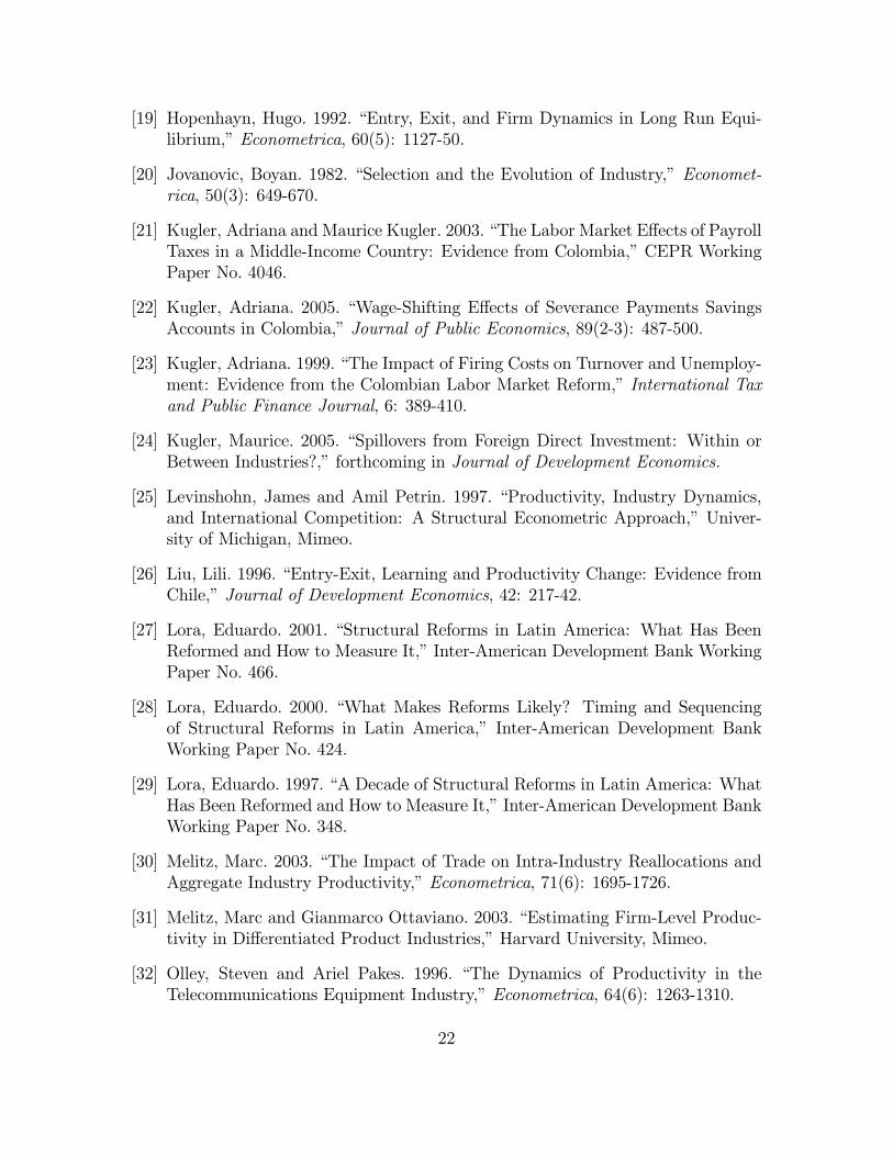
reform index to examine separately the effects of trade and other reforms on plantexits. Our index of reform is generated from the data on institutions collectedby Lora (2001). The reform index, which varies yearly, measures the degree ofmarket orientation in the areas of trade openness, labor regulation, financial system,privatization and taxation. Following Lora (2001), we generate indices of marketreform that separate trade from other reforms, including privatizations as well aschanges in financial and labor markets, and the tax system. We focus on trade reformas opposed to any other reform because the data do not offer enough variability toseparately estimate the effects of different reforms at higher levels of disaggregation,and among all reforms the trade aspect is the one that has received most attentionin Colombia as a key determinant of plant survival.For a given area of reform (such as trade) Lora’s methodology calculates an index

based on relevant subcomponents, each evaluated in a 0-1 scale, where 0 (1) corre-sponds to the most (least) rigid institutions in Latin America over the period for

1Note that the Colombian electoral system at the time ruled out election for more than one term.

5

the corresponding subcomponent.2 Since our focus here is on Colombia, we re-scaleLora indices so that each subcomponent is measured relative to the minimum andmaximum level of reform in Colombia (rather than Latin America) within the period.Figure 1 presents our Trade Reform Index and Other Reform Index, which have anincreasing trend over the period, with an important discrete increase at the beginningof the 1990s for trade reform. Overall, the reform indices suggest that the reformprocess was relatively smooth and successful in reducing distortions from productand factor markets. If the goal of enhancing efficient reallocation in the economywas achieved, its success should be reflected in different exit patterns of plants beforeand after the reforms.

3 Plant-level Data

In this section, we first provide a description of the data and, then, we explain themeasurement of physical productivity and demand shocks.

3.1 Data Description

Our data come from the Colombian Annual Manufacturers Survey (AMS) for theyears 1982 to 1998. The AMS is an unbalanced panel of Colombian plants withmore than 10 employees, or sales above a certain limit (around US$35,000 in 1998).3

The AMS includes information for each plant on: value of output and prices chargedfor each product manufactured; overall cost and prices paid for each material usedin the production process; energy consumption in physical units and energy prices;production and non-production number of workers and payroll; and book values ofequipment and structures.Since we are interested in the effects of efficiency and demand on plant exits, we

need to construct measures of productivity and demand shocks at the plant level. Tothis end, we first estimate total factor productivity (TFP) values for each plant using a

2The trade index has two subcomponents: average tariff, and tariff dispersion (higher averageand dispersion interpreted as more rigid institutions). The “other reforms” index includes: reserverequirements faced by financial institutions; adherence of financial supervision to Bassle minimumcriteria; a measure of interest rate controls; measures of different tax rates and efficiency in thecollection of taxes; a measure of the extent of privatizations of state-owned enterprises; and theextent of layoff costs, restrictions on hiring temporary workers, requirements of higher pay forovertime work, and extent of contributions to social security. Greater financial restrictions, highertax and labor costs, weaker supervision and collection institutions, and lower “stocks” of privatizedfirms, are all interpreted as capturing less developed market institutions.

3In the Appendix to Eslava et al.(2004), we describe in detail the methodology used to generatelongitudinal linkages that allow following plants over time. As explained there, over the periodof study the AMS underwent changes in the sampling and labeling of plants, which require veryinvolved work to generate these linkages and to reduce spurious measurement of entry and exit ofplants.

6

capital-labor-materials-energy (KLEM) production function and demand shock valuesfor each plant using a standard demand function. Thus, we need to construct physicalquantities and prices of output and inputs, capital stock series, and total labor hoursto estimate production functions.

3.1.1 Plant-level Price Indices

With the rich information on prices collected in the AMS, we can construct plant-level price indices for output, materials, and energy. This represents an enormousadvantage with respect to other sources of data, as the use of more aggregate pricedeflators is a common source of measurement error, due to plant-specific demandshocks. Prices of output and materials are constructed using Tornqvist indices. Fora composite of products or materials i of each plant j at time t these Tornqvistindices are the weighted average of the growth in prices for all individual products ormaterials h generated by the plant. This weighted average is given by:

∆Pijt =HXh=1

shjt∆ ln(Phjt),

where i = Y,M, i.e., output or materials,

∆ ln(Phjt) = lnPhjt − lnPhjt−1,

and

shjt =shjt + shjt−1

2

and Phjt and Phjt−1 are the prices charged for product h, or paid for material h, byplant j at time t and t− 1, and sht and sht−1 are the shares of product h in plant j’stotal production, or the shares of material h in the total value of plant j’s materialspurchases, for years t and t− 1.4 The indices for the levels of output (or material)prices for each plant j are then constructed using the weighted average of the growthof prices and fixing 1982 as the base year:

lnPjt = lnPijt−1 +∆Pijt

for t > 1982, where Pj1982 = 100. The price levels are then simply obtained asPijt = exp

lnPijt.5

4The distribution of the weighted average of the growth of prices has large outliers, especially atthe left side of the distribution. In particular, the distribution shows some negative growth ratesof 100% and more. In a country like Colombia, with inflation around 20%, negative growth ratesof these magnitudes seem implausible. For this reason, we trim the 1% tails at both ends of thedistribution as well as any observation with a negative growth rate of prices of more than 50%.

5Given the recursive method used to construct the price indices and the fact that we do not haveplant-level information for product and material prices for the years before plants enter the sample,

7

3.1.2 Capital Stock Series

Given prices for materials and output, the quantities of materials and output areconstructed by dividing the cost of materials and value of output by the correspondingprices. Quantities of energy consumption are directly reported by the plant. Inaddition, we need capital stocks to estimate a KLEM production function.The plant capital stock is constructed recursively on the basis of the expression:

Kjt = (1− δ)Kjt−1 +IjtDt

for all t such that Kjt−1 > 0, where Ijt is gross investment, δ is the depreciation rateand Dt is a deflator for gross capital formation. Our capital stock series includesequipment, machinery, buildings and structures, while excluding vehicles and land.Our measure of Dt is the implicit deflator for capital formation from the input-outputmatrices for years 1982-1994, and from the output utilization matrices for later years.We use the depreciation rates calculated by Pombo (1999) at the 3-digit sectoral level,which range between 8.7% and 17.7% for machinery and between 2.4% and 9.8% forbuildings.Gross investment is generated from the information on fixed assets reported by

each plant, using the expression:

Ijt = KNFjt −KNI

jt − djt − πAjt

where KNFjt is the reported value of fixed assets by plant j at the end of year t, K

NIjt is

the reported value of fixed assets reported by plant j at the start of year t, djt is thedepreciation reported by plant j at the end of year t, and πAit is the reported inflationadjustment to fixed asset value by plant j at the end of year t (only relevant since1995, the first year in which plants were required by law to consider this componentin their calculations of end-of-year fixed assets).The capital stock series is initialized at the year the plant enters the sample, t0.

To obtain the initial value, we use the equation:

Kit0 =KNIit0

12(Dt0 +Dt0−1)

,

where KNIjt0is the first reported nominal capital stock at the beginning of the year.

3.1.3 Labor Hours and Wages

Finally, we construct hours of employment. Since the AMS does not have data onworker hours, we construct a measure of total employment hours at time t for sector

we impute product and material prices for each plant with missing values by using the average pricesin their sector, location, and year. When the information is not available by location, we imputethe national average in the sector for that year.

8

G(j), to which plant j belongs, as,

Hjt =earningsG(j)t

wG(j)t,

where wG(j)t is a measure of sectoral wages at the 3-digit level, and earningsG(j)t isa measure of earnings per worker constructed from our data as

earningsG(j)t =

Pj∈G

payrolljtPj∈G

Ljt

Our measure of wG(j)t is a weighted average of the sector-level wages for productionand non-production workers, where the weights are the shares of each type of workerin total sector employment. The data on wages for each type of worker at the three-digit sector level are obtained from the Monthly Manufacturing Survey. Nominalwages are deflated using CPI.

3.1.4 Descriptive Statistics

Table 1 presents descriptive statistics of the quantity and price variables just de-scribed, for the pre- and post-reform periods. The table reports entry and exit ratesof 9.8% and 8.7% during the pre-reform period, but a lower entry rate of 8.4% anda higher exit rate of 10.7% during the post-reform period.6 The quantity variablesare expressed in logs, while the prices are relative to a yearly producer price indexto discount inflation. Output increased between the pre- and post-reform periods .Similarly, except for labor, input use increased between the pre- and post-reform pe-riods. In particular, the table shows that capital, materials and energy use increasedbetween the pre- and post-reform periods especially for incumbents and entrants. Onthe other hand, labor use decreased between the two periods for entering and exitingplants. Relative prices of output and materials prices declined between the pre- andpost-reform periods for all plants.7 Next, we use these variables to estimate theproduction function and inverse-demand equation.

6These entry and exit rates are lower than those reported for the U.S. and other OECD countries(Davis, Haltiwanger, and Schuh (1996)). Given that the Colombian economy is subject to greaterrigidities, one may indeed expect lower entry and exit rates in the Colombian context (see, e.g.,Tybout (2000) for a discussion of this issue).

7Caution needs to be used in interpreting the aggregate (mean) relative prices in this contextsince the relative price at the micro level is the log difference between the plant-level price and thelog of the aggregate PPI. On an appropriately output weighted basis, the mean of this relativeprice measure should be close to zero in all periods (or one in levels) since the PPI is dominatedby manufacturing industries. The larger difference with respect to PPI in the post-reform periodreflects that the growth of manufacturing prices fell more rapidly than that of other prices in theeconomy, possibly due to the fact that external competition introduced by the reforms affected themanufacturing sector more than others.

9

3.2 Estimation of Productivity and Demand Shocks

We estimate total factor productivity with plant-level physical output data, usingdownstream demand to instrument inputs. In turn, we estimate demand shocks withplant-level price data, using TFP to instrument for output in the demand equation.

3.2.1 Productivity Shocks

We estimate total factor productivity for each establishment as the residual from acapital-labor-energy-materials (KLEM) production function:

Yjt = Kαjt(LjtHjt)

βEγjtM

φjtVjt,

where, Yjt is output, Kjt is capital, Ljt is total employment, Hjt are hours, Ejt isenergy consumption, Mjt are materials, and Vjt is a productivity shock.Our total factor productivity measure is estimated as:

TFPjt = log Yjt − bα logKjt − bβ(logLjt + logHjt)− bγ logEjt − bφ logMjt. (1)

where bα, bβ, bγ, and bφ are the estimated factor elasticities for capital, labor hours,energy, and materials. Since productivity shocks are likely to be correlated withinputs, OLS estimates of factor elasticities are likely to be biased. We thus presentIV estimates, where we use demand-shift instruments which are correlated with inputuse but uncorrelated with productivity shocks. As described in Eslava et al. (2004),we construct Shea (1993) and Syverson (2004) type instruments by selecting industrieswhose output fluctuations are likely to function as approximately exogenous demandshocks for other industries. In addition, we use as instruments one- and two-periodlags of the demand shifters just described, energy and materials prices, and regionalgovernment expenditures in the region where the plant is located.8

Table 2 reports results for the KLEM specification of the production function.Column (1) presents the OLS results from the estimation of the KLEM specification.The results imply elasticities for capital, labor, energy, and materials of about 0.08,0.24, 0.12, and 0.59, respectively. However, as pointed out above, these elasticitiesare likely to be biased if productivity shocks are correlated with input use. Col-umn (2) of Table 2 presents results using 2SLS estimation. Even if we think theinstruments are weakly correlated with productivity shocks, large biases could beintroduced when using IV estimation if the instruments are weakly correlated withthe inputs.9 To check whether inputs are highly and significantly correlated with the

8Sargan tests suggest these are valid instruments, including energy and materials prices whichare unlikely to be affected by buyers’ market power in the Colombian context. See Eslava et al.(2004) for further details on the instruments.

9We also considered other instruments, including longer lags and exponential terms. To selectour baseline instruments, we tested for overidentifying restrictions using a variant of Basmann’s(1960) test, where we estimate a regression of the production function residual on the instruments.

10

instruments, and given that we are considering instrument relevance with multipleendogenous regressors, we report in Column (3) the partial R2 measures suggested byShea (1997) for the first-stages, which capture the correlation between an endogenousregressor and the instruments after taking away the correlation between that partic-ular regressor and all other endogenous regressors.10 The partial R2’s for capital,employment hours, energy, and materials in the KLEM specification are 0.1276, 0.139,0.231, and 0.324, respectively, and 0.2563 and 0.1324 for capital and employment inthe value-added specification, showing that the relevant instruments for each inputcan explain a substantial fraction of the variation in the use of that input. The IVresults in Column (2) of Table 2 also show larger elasticities for capital and energy,but smaller elasticities for labor hours and materials, when inputs are instrumented.The results, thus, indicate that productivity shocks during the period of study arepositively correlated with employment hours and materials and negatively correlatedwith capital and energy.Table 3 reports summary statistics for this and other measures of productivity.

Our productivity measure, which follows the methodology just described, is denotedas “TFP” in the table. Notice, in particular, a high negative correlation of -0.6 of thismeasure with relative output prices, which reveals that high productivity plants arecharacterized by their ability to charge lower prices. Relative output prices in Table3 are measured as the log difference between the plant’s price index and a weightedaverage of the price indices of all plants for the current year, where physical outputshares are used as weights.The importance of using plant-level prices in the estimation of physical efficiency is

evidenced by contrasting “TFP” with the measures of productivity that would resultif output and materials where deflated with sector-level price indices. To calculatethose alternative measures of productivity we construct internally-consistent sectorprices for outputs and inputs, as a weighted average of the plant level prices, wherethe weights are physical output shares. We deflate plant output and/or materialsusing the corresponding sector level deflator, and recalculate productivity using thesealternative measures of output and inputs and the same elasticities reported in Col-umn (2) of Table 2.11 The second row of Table (3) reports summary statistics of an

While lags of more than two periods and exponential terms of the demand shifters turn out to besignificant in these regressions, the rest of our instruments are individually and jointly insignificant.We restrict our instrument list to include those instruments which are not jointly significant in thisregression.10The standard R2 simply reports the square of the sample correlation coefficient between Ijt and

Ijt, where I = K,L,E,M and Ijt are the predicted values of the inputs from a regression of Ijt onthe instruments. The partial R2 reports the square of the sample correlation coefficient between gjtand bgjt, where gjt are the residuals from an OLS regression of Ijt on all other inputs I1jt and bgjtare the residuals from an OLS regression of Ijt on the predicted values of all other inputs I1jt.11Re-estimating the production function using these alternative measures of Yjt and Mjt would

require finding new instruments. The instruments we use for producing Table 2 rely on the assump-tion that a sector’s downstream demand is uncorrelated with its productivity, an assumption that

11

alternative TFP measure that uses sector level deflators for both outputs and inputs(TFP1). Notice that the correlation of this measure with TFP, though high, is farfrom perfect. More interesting, the negative correlation between output prices andphysical efficiency disappears when using this measure of productivity. This stemsfrom the fact that, by ignoring price differentials across plants, this measure of TFPassigns a lower output to low-price plants than the appropriately deflated measuredoes. As we will see below, the ability to identify productivity differentials as move-ments along the demand schedule is key to decomposing the effects of demand andproductivity shocks on a plant’s survival probability. The next two alternatives weinvestigate the respective roles of mismeasuring output (TFP3) vs. inputs (TFP4)when using sector- rather than plant-level price deflators. Comparing the correlationsof TFP with TFP3 and TFP4 shows that the most serious mismeasurement arisesfrom measuring productivity using an output measure based on revenue deflated bya sectoral level output price deflator. By contrast, the high correlation betweenTFP and TFP4 shows that the mismeasurement of inputs using input expendituresdeflated by a sectoral input price deflator yields a measure of productivity that isvery highly correlated with the “true” measure.

3.2.2 Demand Shocks

While productivity is likely to be one of the crucial components of profitability, othercomponents of profitability are also probably important determinants of plant exits.For example, even if plants are highly productive, they may be forced to exit themarket if faced with large negative demand shocks. We capture the demand compo-nent of profitability by estimating establishment-level demand shocks as the residualof the following demand equation:

Yjt = P−εjt Djt,

where Djt is a demand shock faced by firm j at time t and −ε is the elasticity ofdemand.Our demand shock measure is estimated as the residual from estimating this

demand equation,

djt = log cDjt = log Yjt + bε logPjt, (2)

Using OLS to estimate the inverse-demand function is likely to generate an upwardlybiased estimate of demand elasticities because demand shocks are positively correlatedto both output and prices, so that bε will be smaller in absolute value than the trueε. To eliminate the upward bias in our estimates of demand elasticities, we proposeusing TFP as an instrument for Yjt since TFP is positively correlated with output(by construction) but unlikely to be correlated with demand shocks.

is unlikely to hold if plant prices are embedded in the productivity measure.

12

Table 4 reports OLS and IV results of estimating the demand equation.12 OLSresults presented in Column (1) suggest an elasticity of -0.9. Meanwhile, IV results inColumn (2) which use TFP as an instrument for output, show much higher elasticity(in absolute value) of -2.23.13 Finally, note that the last column in Table 4 reportsan R2 for the first stage of close to 0.4, indicating that our instrument explains alarge fraction of price variability.

4 Effects of Market Fundamentals on Plant Exit

According to selection models of industry dynamics (e.g., Jovanovic (1982), Hopen-hayn (1992), Ericson and Pakes (1995), and Melitz (2003)), producers should continueoperations if the discounted value of future profits exceeds the opportunity cost ofremaining in operation. The model we regard as most relevant is the one presentedby Melitz (2003), where a producer with market power makes decisions on outputs,inputs, and output prices, given productivity shocks, demand shocks and input priceshocks drawn by the producer from a joint distribution. Moreover, given fixed costsof operating each period, the producer makes a decision on whether or not to stayor exit at each point in time. In this model (as in other closely related models), theproducer’s exit decisions should be affected by the productivity, demand and inputprice shocks:

ejt =

½1 if PDV {π(Djt, PIjt, TFPjt)}− Cjt < 00 if PDV {π(Djt, PIjt, TFPjt)}− Cjt > 0.

That is, plant j exits if the discounted value of net profits is below the fixed costof operating and the firm exits, and continues in operation if the opposite holds.Profits, π, (and in turn the present discounted value, PDV) are a positive function ofdemand shocks and productivity and a decreasing function of input price shocks.

In practice, we estimate this relationship using a probit model where we spec-ify the probability of exit between t andt + 1 as a function of measures of marketfundamentals in periodt− 1:

Pr(ejst) = λs + δ1TFPjt−1 + δ02PIjt−1 + δ3Djt−1 + ujt, (3)

12The sample size is larger in this table than in Table 2 because the estimations in that tablerequire information on the instruments used for estimating the production function, while demandestimations only require information on output prices, physical output, and TFP estimates.13The negative R-squares for the 2SLS are not surprising and should not be viewed as alarming.

Price and the demand shocks are highly positively correlated. Using the simple demand equation,the variance of output will be equal to terms involving the variance of prices, the variance of demandshocks and a term that depends negatively on the covariance of output and demand shocks. Thus,the variance of demand shocks will exceed the variance of output and, hence, the negative R-squares.

13

where ejst takes the value of 1 if the plant j in sector s exits between periods t andt+ 1; λs are sector effects; TFPjt and Djt are productivity and demand shocks; andPIjt is a vector including energy and materials prices, and ujt is an i.i.d. error term.Table 5 reports summary statistics for the determinants of exit in the equation (3)(except for input prices which are presented in Table1). This table shows morevolatility during the 1990s than the 1980s. Both the means and standard deviationsof total factor productivity and demand shocks increased during the 1990s. At thesame time, both the trade reform index as well as the index for other areas of reformincreased during the 1990s compared to the 1980s. However, the indices suggest thattrade seems to have been liberalized to a much greater extent than other areas.Table 6 reports the results of alternative specifications for the probit models.

Our core specification is reported in Column (3), but we consider some intermediatespecifications to shed light on the sensitivity of the results. In all specifications,we control for 3-digit industry effects and aggregate GDP growth. Starting withthe core specification, we find that higher physical efficiency, lower input prices andhigher demand shocks are all economically and significantly important factors indetermining exit. A rise in productivity by one standard deviation in the previousyear is associated with a fall of 1.4% in the probability of exit in the current year.Increases in energy and materials prices of one standard deviation the previous yearare associated with a rise of about 0.4 % and 1.1% in the probability of exit inthe current year, respectively. We also find that an increase in plant-level demandby one standard deviation in the previous year is associated with a decline of 3.6%in the probability of closing down operations the current year. To appreciate theconsiderable magnitude of these effects note, from Table 1, that the exit rate is below9% in the 1980s and below 11% in the 1990s.To help us understand these results, we consider some intermediate specifications.

In Column (1), we report the results of only including productivity and input priceshocks on the probability of exiting. This specification is of interest because itprovides perspective on the role of productivity and input prices if we neglected orignored output price and demand variation. Column (1) shows that higher produc-tivity and lower materials and energy prices lower the probability of exiting even if weomit both output price and demand variation. In particular, a rise in productivityof one standard deviation in the previous year is associated with a fall of about 1.3%in the probability of exit the current year. Increases in energy and materials pricesthe previous year are also associated with increases of about 0.4 and 0.7% points inthe probability of exit, respectively. The role of productivity and input prices is thusmildly underestimated when demand shocks are excluded.Column (2) adds output prices as an explanatory variable, which is of interest

since output prices may reflect in part quality variation. In the extreme where allwithin industry price variation reflected quality differences, Column (2) would bethe appropriate specification with the interpretation that we would have decomposedquality adjusted productivity into a physical efficiency and a product quality term.

14

Column (2) shows that higher productivity, lower input prices and higher outputprices are associated with a lower probability of exit. It is interesting to compare theimpact of productivity and input prices to both Columns (1) and (3). In comparisonwith Column (1), we find that physical productivity and input prices have a largereffect when controlling for output prices. This pattern is consistent with Table 3,which shows that productivity and output prices are negatively correlated. Then, aplant with low productivity and high input prices is also moving up along the demandschedule. Controlling for output prices, as Column (2) of Table 6 does, isolates theeffect of productivity and input prices from movements along the demand schedule(and effectively also from shifts in this schedule), which go in the opposite direction.This explains the bias in the coefficients associated with productivity and costs inColumn (1), as compared to Column (2).It is also instructive to compare Columns (2) and (3). The productivity and input

price effects in Column (3) are very similar to those in Column (2) and the demandshock variable (which by construction is orthogonal to both the productivity and theinput price effects) has significant explanatory power. Thus, in comparing Columns(2) and (3), it is as though we have decomposed price effects into those effects thatare correlated with movements along the demand schedule (through productivity andinput price effects) and shifts of the demand schedule (through the demand shocks).

4.1 Effects of Market-oriented Reforms

We also explore whether the reforms introduced during the 1990s increased the im-portance of market fundamentals on plant survival. We extend our core specificationby including interactions of productivity, input prices, and demand shocks with thereform indices. In particular, we extend equation (3), by including interactions ofproductivity, input prices, and output prices or demand shocks with the trade reformindex, Tradet, and an index that captures the effects of all other reforms, Othert,during the 1990s in Colombia,

Pr(ejst) = λs + λTRTradet + λOROthert + δ10TFPjt−1

+δ1TRTFPjt−1 × Tradet + δ1ORTFPjt−1 ×Othert (4)

+δ020PIjt−1 + δ02TRPIjt−1 × Tradet + δ02ORPIjt−1 ×Othert+δ30Djt−1 + δ3TRDjt−1 × Tradet + δ3ORDjt−1 ×Othert + ujt.

Table 7 shows results which allow for interactions of market fundamentals withthe reform indices. Column (1) shows the “main” effects (first row of equation(4)), Column (2) shows the interactions with the trade reforms and Column (3)includes the interactions with other reforms (which includes financial market andlabor market reforms). We need to be cautious about interpreting the “main” effectsby themselves because the value of the reform indices is always above zero within our

15

sample. Nevertheless, pushed to their extreme, the “main” effects tell us the impactof market fundamentals if Colombia ever faced such poor institutions that all of thereform indices were equal to zero. Interestingly, Column (1) suggests that even atthis extreme, plants with low productivity, low demand and high input costs are allmore likely to exit. Column (1) also shows the effect of the reform indices consideredindividually. Independent of the state of market fundamentals, trade reforms increasethe likelihood of exit while the other reforms decrease the likelihood of exit. Tradeliberalization increases competition in the product market and this likely explainsreduced plant survival following trade reforms. By contrast, other reforms, includingthe financial reform and tax reforms, reduced credit constraints for plants and thismay explain greater plant survival, especially after financial deregulation.Once we control for the depth of trade and other reforms, a rise in productivity

of one standard deviation in the previous year is associated with a fall of about 1.3%and 1.5% points in the probability of exit during the pre- and post-reform periods,respectively.14 An increase in lagged demand shocks of one standard in the previousyear is associated with a decrease in the likelihood of exit by 4 percent in the pre-reform years and by 3.5 percent in the post-reform years. In terms of input costs,an increase in lagged materials prices of one standard deviation is associated withan increase in the probability of exit of about 0.4% and 1.6% points, pre- and post-reform respectively. Thus, overall there is a general pattern for market fundamentalsto become more important after the market reforms, although this pattern does nothold for demand shocks.The results of interactions with trade reforms in Column (2) suggest that demand

shocks and cost shocks become relatively more important in determining survivalas trade liberalization advances. This means that low demand or small plants aremore likely to exit after trade opening. This is possibly because non-exporting smallplants were the highly protected plants before trade liberalization, or because theseplants are more likely to be credit constrained and thus more likely to suffer cash flowproblems due to intensified competition.By contrast, the results on the interactions with other reforms in Column (3)

indicate increased importance of productivity in determining exits, but less impor-tance of demand and cost shocks as these reforms advance. Greater importanceof productivity after financial and other reforms can be explained by the fact thatimproved financial intermediation probably allows lenders to identify the most pro-ductive projects, thus allowing efficient plants to overcome credit constraints andsurvive more easily.There are a few puzzles in the reported results in Table 7. It is less obvious

why trade liberalization makes physical efficiency less important while other reformsmake demand effects and input cost effects less important. Overall, the reforms taken

14To compute the implied effects in this paragraph, we use the standard deviations in Tables 1and 5 pre- and post-reform for the market fundamentals and evaluate the market reform indices attheir respective pre- and post-reform means.

16

together tend to make market fundamentals more important determinants of exit, soperhaps it is best to think of these in relative terms (e.g., trade reforms increaserole of demand relative to other factors while other reforms increase role of physicalefficiency relative to other factors). Alternatively, we may need a richer modelof market selection with a richer characterization of the covariation and evolution ofdemand shocks, physical efficiency and input price shocks across businesses. Suppose,for example, that young businesses take time to build their market share and also facehigher input prices given their relatively small size, even if they are highly productive.Then, financial market reforms may have made the role of demand and input pricesless relevant as creditors might have been able to take these dynamics into accountand focus to a greater extent on relative productivity which may be a better signalfor long run profitability for young businesses. We leave the investigation of suchricher models of market selection for future work

5 Plant Exits and Aggregate Productivity

In this section, we examine whether market selection and other forms of reallocationare associated with important productivity gains over the period. In particular, wequantify the contribution of allocative efficiency to aggregate productivity by usinga cross-sectional decomposition methodology, first introduced by Olley and Pakes(1996). We quantify what fraction of aggregate productivity every year reflectsaverage productivity and what part reflects the concentration of activity in moreproductive plants, by conducting the following decomposition of aggregate TFP:

TFPt = TFP t +JXj=1

¡fjt − ft

¢ ¡TFPjt − TFP t

¢,

where TFPt is the aggregate total factor productivity measure for a given 3-digitmanufacturing sector in year t.15 These aggregate measures correspond to weightedaverages of our plant-level TFP measures, where the weights are market shares (calcu-lated as described below). The first term of the decomposition, TFP t, is the averagecross-sectional (unweighted) mean of total factor productivity across all plants in thatsector in year t. TFPjt is the total factor productivity measure of plant j at timet estimated as described in Section 3, fjt is the share or fraction of plant j

0s out-put out of sectoral output at the 3-digit level in year t, and f t is the cross-sectionalunweighted mean of fjt. The second term in this decomposition measures whether

15This means that our focus here is on within sector reallocation rather than between sectorreallocation, for sectors defined at the 3-digit level. For measurement and conceptual reasons,comparisons of TFP across sectors (in levels) are more problematic to interpret. Focusing onwithin sector allocation permits us to emphasize the degree to which market reforms have led to animproved allocation of activity across businesses due to higher competition.

17

production is disproportionately located at high-productivity plants and, as such, isa measure of allocative efficiency. Examining this decomposition over time allows usto learn whether the average unweighted productivity as well as allocative efficiencyhas changed, in particular in response to the market reforms.16

In order to evaluate the contribution of net entry, we consider yearly Olley-Pakesdecompositions for three samples. The first sample contains all plants in our dataset,the second sample contains all plants that are continuously in existence for the entiresample period (the balanced sample), and the third sample contains all year-t busi-nesses that are also present in year t-1 and t+1 (three-year continuers). The firstsample provides perspective on the role of allocative efficiency for all plants. Sinceallocative efficiency can improve either through entry and exit or through reallocationof activity among continuing plants, the next two samples provide perspective aboutthe role of net entry. In particular, while the balanced panel decomposition providesinformation about long lived continuously operating plants, the sample of three-yearcontinuers contains some businesses that, while not in their first or last year, haveentered recently or are about to exit.Table 8 shows the results of this exercise. For each sample, the table reports the

value of each term of the Olley-Pakes decomposition for the average three-digit sector.For the sample including all plants (Columns (1)-(3)), we see that aggregate industryproductivity increased substantially over the sample period. For the average industry,productivity increased by 30 log points from 1982 to 1998. The decomposition showsthat most of this increase, 21 out of the 30 points, is accounted for by an increasein allocative efficiency. Interestingly, the unweighted average component increasedduring the 1980s but actually fell during the 1990s. In contrast, the increase inallocative efficiency is concentrated in the 1990s, after the market reforms.The balanced panel shows similar qualitative patterns with a large role for al-

locative efficiency especially in the 1990s. Thus, allocative efficiency improved evenamong long lived plants following market reforms. Interestingly, this sample actu-ally shows a decline in the productivity of the average plant over the period. For thethree-year continuers, we also observe the allocative efficiency term dominating theincrease in productivity during the 1990s.Comparing the dynamics of aggregate productivity across the three samples yields

some insights on the role of net entry. For the period for which all samples areavailable (1983-97), we see that the whole sample and the three-year continuer sampleexhibit an increase in aggregate productivity of about 25 log points, but the balancedpanel exhibits only a 14 point increase in productivity. However, all three samplesexhibit about a 15 point increase in allocative efficiency. Thus, the difference acrossthe samples is largely in the unweighted productivity component. This providesevidence of a productivity enhancing effect of plant turnover, as the difference across

16An advantage of this cross-sectional method over methods that decompose changes in pro-ductivity over time, is that cross-sectional differences in productivity are more persistent and lessdominated by measurement error or transitory shocks.

18

samples is, by construction, explained by the effect of entry and exit. While we havenot focused here on the contribution of entry, part of the contribution of entry andexit is inherently related to whether productivity is an important determinant of exit.That is, exit will by construction raise the average unweighted productivity of theremaining plants for all plants and the three-year continuer samples, if and only if, it isthe low productivity plants that exit. By contrast, this market selection contributionto the unweighted average is, by construction, not present in the balanced sample.Moreover, the fact that the growth of average productivity is similar in the wholesample and the sample of three-year continuers reveals that the contribution of entryand exit takes time and it does not simply refelect the contribution of turnover toproductivity by very young plants (i.e., plants less than 3 years old).The results of productivity decompositions, thus, reveal three related phenomena.

First, the increase in average productivity in our whole sample is very much asso-ciated with an improvement in allocative efficiency. Second, the rise in aggregateproductivity among incumbents throughout the sample period is fully accounted forby the expanding sectoral market share for relatively efficient plants at the expenseof shrinking sectoral market share for relatively inefficient ones. Third, the contri-bution of entry and exit is both via the increased market shares of more productivitybusinesses but also through the impact of market selection on average unweightedproductivity. Hence, these findings suggest that within sector reallocation and se-lection, at the 3-digit level, combined together account for aggregate productivitygrowth over the 1980s and 1990s in Colombian manufacturing.

6 Conclusion

Plant exit is an essential aspect of market selection. We have characterized the roleof input costs, physical efficiency and demand in determining the likelihood of plantsurvival. We find that each of these three components plays an important role inexplaining the probability of survival the following year.We also examined the impact of market-oriented reforms on plant survival. While

trade liberalization increases plant exit, financial and other reforms reduce the prob-ability of exit. In addition, we find that trade liberalization increases the likelihoodof exit for plants facing low demand and relatively high input prices. By contrast,financial and other reforms increase the role of efficiency and reduce the role of de-mand and input prices in determining plant survival. Trade liberalization squeezesout of operation plants with low profit margins. At the same time, improved factormarket flexibility (capital and labor market deregulations) and private sector incen-tives (lower tax burdens and privatization) make plant physical efficiency relativelymore important in accounting for plant survival relative to demand and input prices.This is probably due to more productive plants being able to expand at the expenseof less productive ones.We find that average productivity increased in the average 3-digit industry and

19

that improvements in allocative efficiency are the primary driving force of this im-provement. Our results suggest that plant entry and exit play a substantial rolebut that improved allocative efficiency amongst long-lived plants is also important.One issue for future research is to disentangle the respective contributions of im-provement in allocative efficiency for continuing, entering and exiting plants. Suchan investigation requires capturing the impact of market reforms on adjustment dy-namics of continuing, entering and exiting businesses. A complicating factor in suchan investigation is the recognition that all these dynamics are closely related — forexample, an important component of the adjustment of continuing businesses mightbe the post-entry growth dynamics of young businesses as well as the exit of youngbusinesses.Our analysis of market reforms can be pushed in additional interesting directions

as well. We use broad based measures of market reforms to examine the interactionof micro fundamentals and economy-wide reforms on market selection. We havenot yet investigated how plants with observably different characteristics (e.g., youngand small businesses) might have responded differentially to the market reforms. Ina like manner, we have not yet investigated the extent to which market reformsthemselves differ substantially across sectors or apply differently to businesses ofobservably different characteristics. We leave this investigation for future work.

References

[1] Aw, Bee-Yan, Siaomin Chen, and Mark Roberts. 1997. “Firm-level Evidence onProductivity Differentials, Turnover and Exports in Taiwanese Manufacturing,NBER Working Paper 6235.

[2] Baily, Martin, Charles Hulten and David Campbell. 1992. “Productivity Dynam-ics in Manufacturing Establishments,” Brookings Papers on Economic Activity:Microeconomics, 187-249.

[3] Bartelsman, Eric and Mark Doms. 2000. “Understanding Productivity: Lessonsfrom Longitudinal Microdata,” Journal of Economic Literature, 38(2): 569-594.

[4] Bartelsman, Eric and Phebus Dhrymes. 1998. “Productivity Dynamics: U.S.Manufacturing Plants 1972-1986,” Journal of Productivity Analysis, 9(1): 5-34.

[5] Bartelsman, Eric, Ricardo Caballero and Richard Lyons. 1994. “Customer- andSupplier-Driven Externalities,” American Economic Review, 84(4): 1075-1084.

[6] Basmann, Robert. 1960. “On Finite Sample Distributions of Generalized Clas-sical Linear Identifiability Test Statistics,” Journal of the American StatisticalAssociation, 55: 650-659.

20

[7] Basu, Susanto and John Fernald. 1997. “Returns to Scale in U.S. Production:Estimates and Implications,” Journal of Political Economy, 105(2): 249-283.

[8] Bigsten, Arne, Paul Collier, Stefan Dercon, Bernard Gauthier, Jan Gunning An-ders Isaksson, Abena Oduro, Remco Oostendrop, Cathy Pattillo, Mans Soder-bom, Michel Sylvain, Francis Teal and Albert Seufack. 1997. “Exports and Firm-level Efficiency in the African Manufacturing Sector,” University of Montreal.

[9] Chen, Tain-jy and De-piao Tang. 1987. “Comparing Technical Efficiency Be-tween Import-Substitution-Oriented and Export-Oriented Foreign Firms in aDeveloping Country,” Journal of Development Economics, 36: 277-289.

[10] Davis, Steven, John Haltiwanger and Scott Schuh. 1996. Job Creation and De-struction. Cambridge, Mass.: MIT Press.

[11] Edwards, Sebastian. 2001. The Economic and Political Transition to an OpenMarket Economy: Colombia. Paris: OECD.

[12] Ericson, Richard and Ariel Pakes. 1995. “Markov-Perfect Industry Dynamics: AFramework for Empirical Work,” Review of Economic Studies, 62(1): 53/82.

[13] Eslava Marcela, John Haltiwanger, Adriana Kugler and Maurice Kugler. 2004.“The Effects of Structural Reforms on Productivity and Profitablity EnhancingReallocation: Evidence from Colombia,” Journal of Development Economics,75(2): 333-371.

[14] Eslava Marcela, John Haltiwanger, Adriana Kugler and Maurice Kugler. 2005.“Employment and Capital Adjustments after Factor Market Deregulation: PanelEvidence from Colombian Plants,” Mimeo.

[15] Foster, Lucia, John Haltiwanger, and Chad Syverson. 2003. “Reallocation, FirmTurnover, and Efficiency: Selection on Productivity or Profitability?,” Univer-sity of Maryland, Mimeo.

[16] Foster, Lucia, John Haltiwanger, and Cornell Krizan. 2001. “Aggregate Produc-tivity Growth: Lessons from Microeconomic Evidence,” in Edward Dean MichaelHarper and Charles Hulten, eds., New Developments in Productivity Analysis.Chicago: University of Chicago Press.

[17] Hall, Robert. 1990. “Invariance Properties of Solow’s Productivity Residual,”in Peter Diamond, ed., Growth/Productivity/Unemployment. Cambridge: MITPress.

[18] Harrison, Ann. 1994. “Productivity, Imperfect Competition, and Trade Reform:Theory and Evidence,” Journal of International Economics, 36: 53-73.

21

[19] Hopenhayn, Hugo. 1992. “Entry, Exit, and Firm Dynamics in Long Run Equi-librium,” Econometrica, 60(5): 1127-50.

[20] Jovanovic, Boyan. 1982. “Selection and the Evolution of Industry,” Economet-rica, 50(3): 649-670.

[21] Kugler, Adriana and Maurice Kugler. 2003. “The Labor Market Effects of PayrollTaxes in a Middle-Income Country: Evidence from Colombia,” CEPR WorkingPaper No. 4046.

[22] Kugler, Adriana. 2005. “Wage-Shifting Effects of Severance Payments SavingsAccounts in Colombia,” Journal of Public Economics, 89(2-3): 487-500.

[23] Kugler, Adriana. 1999. “The Impact of Firing Costs on Turnover and Unemploy-ment: Evidence from the Colombian Labor Market Reform,” International Taxand Public Finance Journal, 6: 389-410.

[24] Kugler, Maurice. 2005. “Spillovers from Foreign Direct Investment: Within orBetween Industries?,” forthcoming in Journal of Development Economics.

[25] Levinshohn, James and Amil Petrin. 1997. “Productivity, Industry Dynamics,and International Competition: A Structural Econometric Approach,” Univer-sity of Michigan, Mimeo.

[26] Liu, Lili. 1996. “Entry-Exit, Learning and Productivity Change: Evidence fromChile,” Journal of Development Economics, 42: 217-42.

[27] Lora, Eduardo. 2001. “Structural Reforms in Latin America: What Has BeenReformed and How to Measure It,” Inter-American Development Bank WorkingPaper No. 466.

[28] Lora, Eduardo. 2000. “What Makes Reforms Likely? Timing and Sequencingof Structural Reforms in Latin America,” Inter-American Development BankWorking Paper No. 424.

[29] Lora, Eduardo. 1997. “A Decade of Structural Reforms in Latin America: WhatHas Been Reformed and How to Measure It,” Inter-American Development BankWorking Paper No. 348.

[30] Melitz, Marc. 2003. “The Impact of Trade on Intra-Industry Reallocations andAggregate Industry Productivity,” Econometrica, 71(6): 1695-1726.

[31] Melitz, Marc and Gianmarco Ottaviano. 2003. “Estimating Firm-Level Produc-tivity in Differentiated Product Industries,” Harvard University, Mimeo.

[32] Olley, Steven and Ariel Pakes. 1996. “The Dynamics of Productivity in theTelecommunications Equipment Industry,” Econometrica, 64(6): 1263-1310.

22

[33] Pack, Howard. 1984. Productivity, Technology, and Industrial Development: ACase Study in Textiles. New York: Oxford University Press.

[34] Pombo, Carlos. 1999. “Productividad Industrial en Colombia: Una Aplicacionde Numeros Indices,” Revista de Economia del Rosario.

[35] Roberts, Mark and Dylan Supina. 1996. “Output Price, Markups, and ProducerSize,” European Economic Review, 40(3-5): 909-21.

[36] Roberts, Mark and Dylan Supina. 1996. “Output Price and Markup Dispersionin Microdata: The Roles of Producer Heterogeneity and Noise,” in Michael Baye,ed., Advances in Applied Microeconomics, Vol. 9. JAI Press.

[37] Roberts, Mark and James Tybout. 1996. Industrial Evolution in DevelopingCountries: Micro Patterns of Turnover, Productivity and Market Structure. NewYork: Oxford University Press.

[38] Shea, John. 1997. “The Input-Output Approach to Instrument Selection,” Jour-nal of Business and Economic Statistics, 11(2): 145-155.

[39] Shea, John. 1993. “Do Supply Curves Slope Up?” Quarterly Journal of Eco-nomics, 108(1): 1-32.

[40] Syverson, Chad. 2004. “Market Structure and Productivity: A Concrete Exam-ple,” Journal of Political Economy, 112(6): 1181-1233.

[41] Syverson, Chad. 2002. “Price Dispersion: The Role of Product Substitutabilityand Productivity,” University of Chicago, Mimeo.

[42] Tybout, James. 2000. “Manufacturing Firms in Developing Countries: How WellDo They Do, And Why?, Journal of Economic Literature, 38(1): 11-34.

[43] Tybout, James and Daniel Westbrook. 1995. “Trade Liberalization and Dimen-sions of Efficiency Change in Mexican Manufacturing Industries,” Journal ofInternational Economics, 39(1-2): 53-78.

23

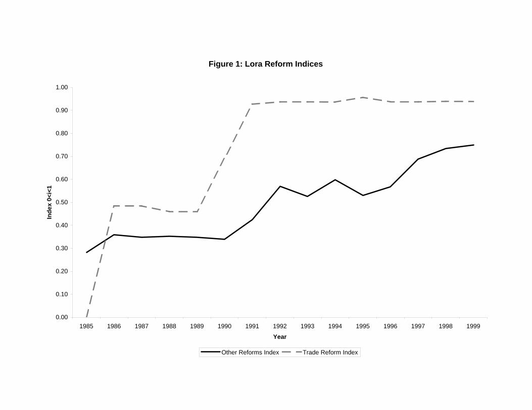
Figure 1: Lora Reform Indices

0.00

0.10

0.20

0.30

0.40

0.50

0.60

0.70

0.80

0.90

1.00

1985 1986 1987 1988 1989 1990 1991 1992 1993 1994 1995 1996 1997 1998 1999

Year

Inde

x 0<

i<1

Other Reforms Index Trade Reform Index

Table 1: Descriptive Statistics, Before and After Reforms

Variable Pre-Reforms Post-Reforms

Output 10.49 (1.67)

10.90 (1.88)

Capital 8.21 (2.05)

8.75 (2.18)

Labor 10.97 (1.1)

10.95 (1.25)

Energy 11.30 (1.88)

11.55 (1.99)

Materials 9.61 (1.85)

10.25 (1.88)

Output Prices -0.08 (0.44)

-0.15 (0.74)

Energy Prices 0.25 (0.50)

0.55 (0.43)

Material Prices

0.02 (0.35)

-0.10 (0.57)

Entry Rate 0.0981 0.0843 Exit Rate 0.0873 0.1069 N 55,298 44,816

Notes: This table reports means and standard deviations of the log of quantities and of log price indices deviated from yearly log producer price indices. The entry and exit rates are the number of entrants divided by total plants and number of exiting plants divided by total number of plants. A plant that enters in t is defined as a plant present in t but not in t-1, while a plant that exits in t is one that is present in t but not in t+a. The pre-reform period includes the years 1982-90 and the post-reform period includes the years 1991-98.

Table 2: Production Function Equations

OLS

(1)

2SLS

(2)

First Stage R²

(3)

Capital 0.0764

(0.0025) 0.3027

(0.0225) 0.128

Labor Hours 0.2393 (0.0037)

0.2125 (0.0313)

0.139

Energy 0.124 (0.0028)

0.1757 (0.0143)

0.231

Materials 0.5891 (0.0026)

0.2752 (0.0095)

0.324

R² 0.8621 0.8107 - N 48,114 48,114 -

Notes: Standard errors are reported in parentheses. The regressions in Columns (1) and (2) use physical output as the dependent variable, and capital, employment hours, energy, and materials as regressors, where all variables are in logs. For Column (2), the following variables are used to instrument the inputs: downstream demand instruments constructed as the demand for the intermediate output (calculated using the input-output matrix); one- and two-period lags of downstream demand; regional government expenditures, excluding government investment; and energy and material plant-level prices, deviated from the yearly PPI. The first partial R² reports the sample correlation coefficient between sjt and ŝjt, where sjt are the residuals from a regression of Ijt on all other inputs I1jt and ŝjt are the correlations between Îjt and the predicted values of all other inputs Î1jt.

Table 3: Descriptive Statistics of Different TFP Measures

Correlation Coefficients Matrix

TFP Measure

Mean and SD TFP

TFP2 TFP3 TFP4 RP1

TFP

1.0873 (0,765)

1 [86,251]

0.7048 [86,251]

0.6958 [86,251]

0.9885 [86,251]

-0.6310 [86,251]

TFP - Sector-level Output and Materials Prices (TFP2)

1.2123 (0.612)

1 [86,251]

0.9821 [86,251]

0.6973 [86,251]

-0.0081 [86,251]

TFP – Only Sector-level Output Prices (TFP3)

1.2172 (0.622)

1 [86,251]

0.6604 [86,251]

0.0220 [86,251]

TFP - Only Sector-level Materials Prices (TFP4)

1.0824 (0.772)

1 [86,251]

-0.6504 [86,251]

Output Prices relative to PPI (RP1)

-0.1201 (0.545)

1 [86,251]

This table reports means, standard deviations and correlation coefficients for different measures of TFP and for the plant-level output prices. Al figures are simple means of three-digit sector statistics. Numbers of observations for the calculation of correlation coefficients are reported in square parentheses. All measures of TFP are calculated using the factor elasticities reported in column (2) of Table 2. Alternative measures of TFP use output and materials deflated with either the plant-level price index or an internally consistent sector-level price index. The latter is calculated at the three-digit level as the geometric mean of plant tlevel indices, using output shares as weights.Relative output prices are constructed as the log difference between the plant's price index and an aggregate log price index. The latter is the Producer Price Index in RP1, and the weighted mean of plant-level prices (where the weights are physical output shares) for RP2.

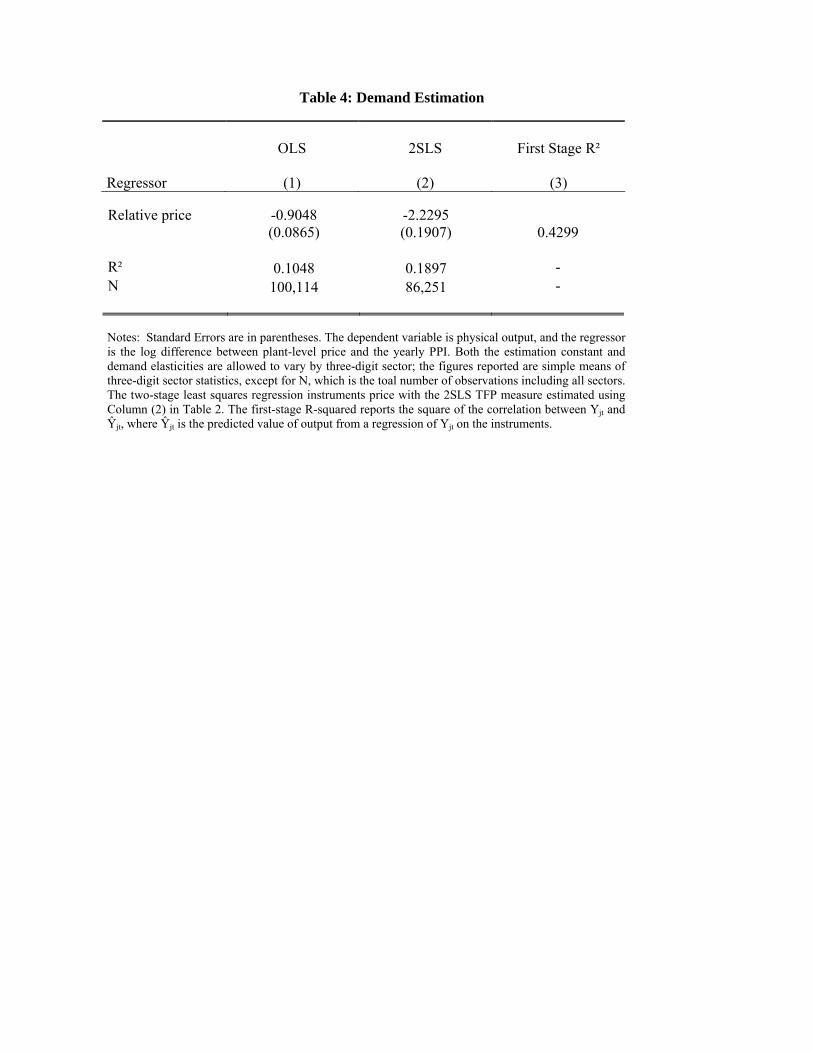
Table 4: Demand Estimation

Regressor

OLS

(1)

2SLS

(2)

First Stage R²

(3)

Relative price -0.9048

(0.0865) -2.2295 (0.1907) 0.4299

R² 0.1048 0.1897 - N 100,114 86,251 -

Notes: Standard Errors are in parentheses. The dependent variable is physical output, and the regressor is the log difference between plant-level price and the yearly PPI. Both the estimation constant and demand elasticities are allowed to vary by three-digit sector; the figures reported are simple means of three-digit sector statistics, except for N, which is the toal number of observations including all sectors. The two-stage least squares regression instruments price with the 2SLS TFP measure estimated using Column (2) in Table 2. The first-stage R-squared reports the square of the correlation between Yjt and Ŷjt, where Ŷjt is the predicted value of output from a regression of Yjt on the instruments.

Table 5: Descriptive Statistics of Determinants of Survival, Before and After Reforms

Variable Pre-Reforms Post-Reforms

TFP 1.1014 (0.6754)

1.1414 (0.8612)

Demand 10.4966 (1.9119)

10.7824 (2.1303)

Trade Reform 0.4362 (0.2046)

0.9384 (0.0088)

Other Reforms 0.3391 (0.0247)

0.5403 (0.0642)

N 55,298 44,816

Notes: This table reports means and standard deviations. The TFP measured is obtained using the factor elasticities estimated in Column (2) of Table 2, and the measure of Demand Shocks is obtained using the sector-level demand elasticities summarized in Column (2) of Table 4. The Trade Reform Index is the Lora Trade Reform Index, where each of its sub-components has been re-scaled to be 0 in the year of less liberalization and 1 in the year of most liberalization. The Index of Other Reforms is constructed in a similar fashion using all components of the Lora Overall Reform Index, except those included in the Trade Index.

Table 6: Determinants of Exit Probability

(1) (2) (3)

Lagged Productivity -0.0167

(0.0046) -0.0298 (0.009)

-0.0179 (0.0077)

Lagged Energy Prices

0.0078 (0.0022)

0.0087 (0.0026)

0.0085 (0.0041)

Lagged Materials Prices

0.0155 (0.0044)

0.0236 (0.0072)

0.0238 (0.0103)

Lagged Output Prices

-

-0.029 (0.0088)

-

Lagged Demand Shock

-

-

-0.018 (0.0078)

Sector effects YES YES YES GDP growth YES YES YES

Likelihood Ratio 642.2 (35 df) 751 (36 df) 1,516.6 (36 df)

N 57,515 57,515 57,515

Notes: Standard errors in parentheses. This table reports marginal effects from a Probit estimation of the probability of exit, where exit is 1 for plant i in year t if the plant produced in year t but not in year t+1. All specifications include sector effect at the three-digit level, and growth of GDP, as well as plant-level productivity, energy prices, and materials prices. Column (2) includes output prices, and column (2) includes a measure of demand shocks estimated using column (2) in Table 4.

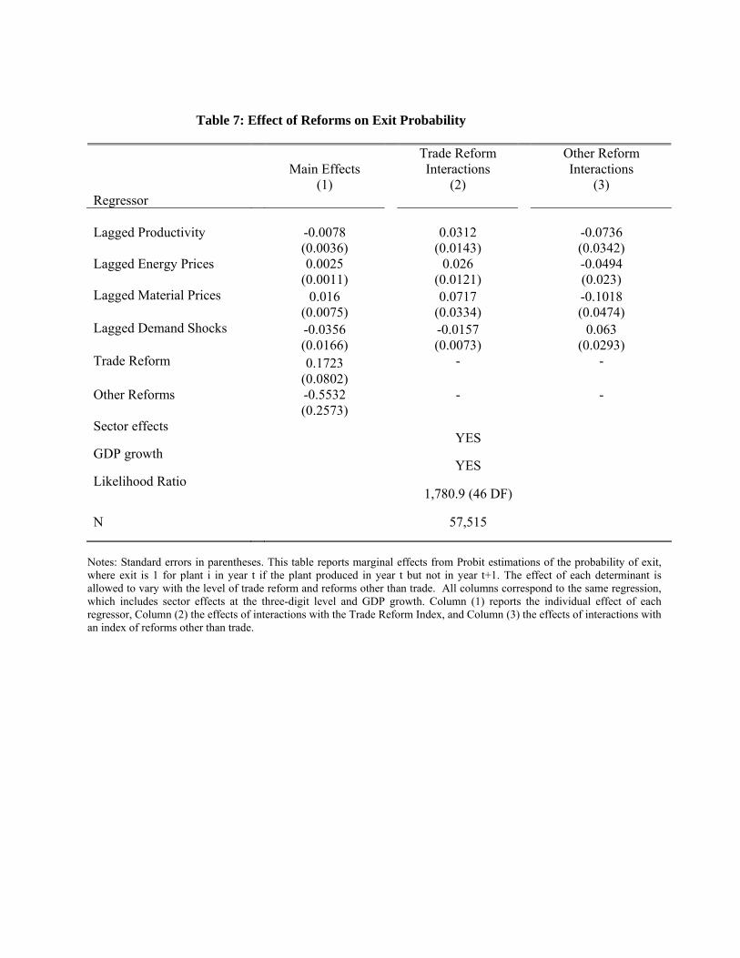
Table 7: Effect of Reforms on Exit Probability

Regressor

Main Effects

(1)

Trade Reform Interactions

(2)

Other Reform Interactions

(3)

Lagged Productivity -0.0078

(0.0036) 0.0312

(0.0143) -0.0736

(0.0342) Lagged Energy Prices 0.0025

(0.0011) 0.026

(0.0121) -0.0494

(0.023) Lagged Material Prices 0.016

(0.0075) 0.0717

(0.0334) -0.1018

(0.0474) Lagged Demand Shocks -0.0356

(0.0166) -0.0157 (0.0073)

0.063 (0.0293)

Trade Reform 0.1723 (0.0802)

- -

Other Reforms -0.5532 (0.2573)

- -

Sector effects YES

GDP growth YES

Likelihood Ratio 1,780.9 (46 DF)

N 57,515

Notes: Standard errors in parentheses. This table reports marginal effects from Probit estimations of the probability of exit, where exit is 1 for plant i in year t if the plant produced in year t but not in year t+1. The effect of each determinant is allowed to vary with the level of trade reform and reforms other than trade. All columns correspond to the same regression, which includes sector effects at the three-digit level and GDP growth. Column (1) reports the individual effect of each regressor, Column (2) the effects of interactions with the Trade Reform Index, and Column (3) the effects of interactions with an index of reforms other than trade.

Table 8: Aggregate Productivity Decompositions

for Different Samples

Overall Sample Balanced panel Three-year continuers

Weighted Simple Average

Cross-term

Weighted Simple Average

Cross-term

Weighted Simple Average

Cross-term

Year (1) (2) (3) (4) (5) (6) (7) (8) (9) 1982 1.34 1.01 0.33 1.39 1.12 0.27 - - - 1983 1.35 0.97 0.38 1.38 1.08 0.31 1.36 0.99 0.37 1984 1.31 0.98 0.33 1.34 1.09 0.26 1.32 1.02 0.30 1985 1.38 1.06 0.33 1.42 1.13 0.29 1.38 1.07 0.32 1986 1.39 1.11 0.28 1.41 1.19 0.22 1.39 1.12 0.27 1987 1.42 1.13 0.29 1.42 1.18 0.24 1.41 1.13 0.28 1988 1.48 1.19 0.29 1.45 1.23 0.22 1.47 1.19 0.28 1989 1.46 1.17 0.29 1.45 1.21 0.24 1.45 1.17 0.27 1990 1.51 1.16 0.35 1.49 1.20 0.29 1.51 1.18 0.33 1991 1.54 1.17 0.36 1.54 1.21 0.33 1.53 1.17 0.37 1992 1.52 1.11 0.41 1.47 1.16 0.31 1.50 1.14 0.36 1993 1.48 1.11 0.38 1.46 1.13 0.33 1.48 1.12 0.36 1994 1.53 1.09 0.44 1.48 1.10 0.38 1.52 1.09 0.43 1995 1.52 1.02 0.50 1.48 1.07 0.40 1.52 1.05 0.47 1996 1.59 1.01 0.58 1.49 1.06 0.43 1.58 1.06 0.52 1997 1.60 1.07 0.53 1.52 1.06 0.46 1.60 1.09 0.51 1998 1.64 1.10 0.54 1.51 1.05 0.46 - - -

Notes: All figures are simple means of 3-digit sector level statistics. Columns (1), (4) and (7) show aggregate TFP, calculated as the weighted mean of TFP, where the weight for each plant is its share in corresponding three-digit level sector output. Columns (2), (5) and (8) show the contribution to aggregate productivity of average TFP. Columns (3), (6) and (9) show the contribution of the cross-sectional correlation between plant-level market share and TFP.