Pipe Line Calculations

Chapter 7Pipeline Calculations

7.1 Pipeline Calculations

The performance of a pump in a piping system is determined by the pipeline char-acteristics. A single pump will deliver different flow rates and heads when installedin two different pipelines. Therefore, the characteristic behavior of a piping systemon which the pump(s) are installed must be determined before any pump selectionis started. In the next section, the methods for calculating the pressure losses in thestraight pipes as well as in different common fittings installed in a piping systemwill be presented.

7.1.1 Bernoulli’s Equation

Bernoulli’s equation which basically describes the energy conservation law for in-viscid flows in a piping system is used to obtain the characteristic curve of a system.According to this law,

if in a non-compressible flow, the pressure losses in the system are neglected, no externalenergy is given to the liquid, and liquid does not transfer energy to an external source,the total energy of the system between two points of the flow on one streamline remainsconstant.

Therefore, between any two points in the flow, e.g. points 1 and 2, one can write

P1

γ+ V 2

1

2g+ Z1 = P2

γ+ V 2

2

2g+ Z2 = cte (7.1)

However, for a system of pipelines, there are always energy losses in the pipesand fittings. Thus, Bernoulli’s equation for two different points of the pipeline canbe written as

P1

γ+ V 2

1

2g+ Z1 = P2

γ+ V 2

2

2g+ Z2 + HL12 (7.2)

82

7.2 Pressure Loss Calculation in Straight Pipes 83

where HL12 is the pressure loss between points 1 and 2 with a unit of meter in SIunit system.

7.1.2 Pressure Loss

The pressure losses occur due to the friction of the liquid particles against each other(shear forces) and the pipe walls. Due to this friction, there would be a significantenergy loss that could have been transferred to the useful work. In other words, therewould be always a static pressure loss, in the direction of flow that can be measuredwith a pressure gauge.

In general, the pressure losses appear in two forms in a piping system:

1. Pressures losses in straight pipes, which are also called linear pressure losses.2. Pressure losses in valves, bends, and other pipe fittings, which are called local

pressure losses.

As will be presented later, if the pipe diameter and the flow rate remain constantin a straight piping system, the pressure loss in that straight pipe will change linearlywith increasing pipe length, i.e. the slope of the pressure loss remains constant.

The pressure losses in the valves and other fittings in the pipeline are generatedfrom two sources:

• The pressure losses due to the liquid friction at the walls of the fittings. Whenthe fittings also change the direction of the fluid flow, like bends or some typesof valves, the flow would be disturbed and more pressure loss is generated.

• The pressure losses that are generated in the straight parts of the pipe due to theexistence of a fitting or change in the pipe diameter. Because of the fittings, thefluid flow is disturbed and that would increase the pressure loss in the straightpart of the pipe.

7.2 Pressure Loss Calculation in Straight Pipes

7.2.1 Darcy-Weisbach Formula

The Darcy-Weisbach relation is one of the basic equations for calculating the pres-sure loss and can be written as

HL = fL

D× V 2

2g(7.3)

In this relation, HL is the pressure loss, L is the length of the pipe, D is theinternal diameter of the pipe (all in meters), V is the average velocity of the flow

84 7 Pipeline Calculations

(Flow rate/Pipe Cross Section) in m/s, f is the friction coefficient, and g is thegravitational acceleration in m/s2. The above equation can be written as

ΔP = fL

D× ρ

V 2

2(7.4)

whereΔP is the pressure loss, and ρ is the density of the liquid. The Darcy equationcan be used for any flow regime, laminar or turbulent flow. Equation (7.4) can beused for calculating the pressure loss in the pipes with constant diameter and liquidswith constant velocity and density. For cases in which the liquid conditions aredifferent in different sections of the pipe, the pressure loss can be calculated foreach section, using the diameter and flow conditions for that section of the pipe.These losses can then be added together to obtain the total pressure loss.

7.2.2 Reynolds Number

The Reynolds number is the ratio of inertial forces (Vρ) to the viscous forces (μ/L)in a flow and is used for determining whether a flow will be laminar or turbulent. Itis named after Osborne Reynolds (1842–1912), who in 1883 after studying differentfluid flow regimes presented two distinctive types of flows.

1. Laminar flow: in this flow regime, the liquid particles move along parallel linesand do not get mixed.

2. Turbulent flow: in this flow regime, the flow lines are not parallel and the liquidparticles get mixed as they move.

To determine whether a flow is laminar or turbulent in a pipeline, one shouldcalculate the Reynolds number as defined below:

Re = ρV D

μ(7.5)

where V is the flow velocity in m/s, D is the pipe diameter in meter, andμ is the dy-namic viscosity of the liquid in kg/ms. The Reynolds number Re is non-dimensional.

For laminar flows Re ≤ 2000 and for turbulent flows Re > 4000. It is possi-ble that with higher Reynolds numbers, more than 4000, the flow remains laminar.But these conditions apply only in the labs and in most industrial applications thetwo above limits really exist. The flow regime corresponding to Reynolds numberbetween 2000 and 4000 is called the transitional flow.


7.2.3 Friction Factor

The friction factor for different flow regimes is different:

a. For laminar flows, Re ≤ 2000, the friction factor is only a function of theReynolds number and can be obtained from

f = 64

Re= 64ν

DV(7.6)

By using this value in the pressure drop (7.4), one can see that

ΔP = 32LVμ

D2or HL = 32

νLV

g D2(7.7)

b. For turbulent flows, Re > 4000, the friction factor is a function of the Reynoldsnumber, and also depends on the relative roughness of the pipe walls, i.e. ε

D .ε is the roughness of the walls and D is the internal diameter of the pipe (insome references symbol K is also used to specify the wall roughness). One ofthe most commonly used theoretical relation for calculating the friction factorin turbulent flows is Colebrook-Prandtl relation. This relation which also has agood agreement with experiments is presented as

1√f

= −2 log

(2.51

Re√

f+ ε

D× 1

3.71

)(7.8)

In those cases where the Reynolds number is much higher compared to the rel-ative roughness, the first term inside the bracket can be ignored. This means forvery rough pipes, the friction factor is only dependent on the relative roughness(in other words, the wall roughness would be larger than the boundary layerwhich affects the fluid flow). For these cases the friction factor can be obtainedfrom

1√f

= 1.14 − 2 logε

D(7.9)

In those pipes that are hydraulically smooth (ε ≈ 0), such as glass or brasspipes, the effect of the wall roughness is much smaller than the Reynolds number;therefore, the friction factor can be obtained from (Darcy equation)

1√f

= 2 log

(Re

√f

2.51

)or f = 0.36 Re−1/4 (7.10)

c. In the transient regime, 2000 < Re < 4000, the friction factor is unknown andits value depends on the laminar flow conditions for the low Reynolds numbersand on the turbulent flow conditions at higher Reynolds numbers.


In pipes with non-circular cross sections, the equivalent or hydraulic diametermust be used in all calculations. The hydraulic diameter can be obtained from

Dh = 4A

S(7.11)

where Dh is the hydraulic diameter, A is the cross-sectional area of the pipe, andS is the wetted perimeter. In open canals, the hydraulic diameter can be used withgood accuracy.

Since the application of (7.6–7.10) for calculating the friction factor is notstraightforward in many cases, usually friction factors are presented in the formof charts or diagrams. One of the best and fundamental charts for calculatingthe friction factor is the Moody Diagram, presented in Fig. 7.1. In this diagramthe friction factor f is presented based on the Reynolds number and the relativeroughness.

The relative roughness, εD , for new pipes and different materials can be also

obtained from Fig. 7.2.There is also another diagram for calculating the pressure loss directly from the

friction factors of Colebrook, which is presented in Fig. 7.3. From this curve, thepressure losses for every 100 m of a straight pipe based on the mass flow rate andpipe diameter (velocity) can be obtained. This diagram is prepared for new cast-iron pipes. When the wall roughness and material of the pipe are different withthese conditions, the pressure loss can be corrected by multiplying it by the numberspresented in Table (7.1).

Fig. 7.1 The friction factor in the pipes (Moody Diagram) [1]


Fig. 7.2 The relative roughness and the friction factor for commercial pipes for fully turbulentflows. Taken from ASME and prepared by L.F. Moody. (English Units) [2]


Fig. 7.3 Pressure loss in new cast iron straight pipes. Water temperature is 20 ◦C [3].


Table 7.1 Pressure loss factor for different pipe roughness [3]

Pipe type Multiple by

For new steel pipes 0.8For very rough pipes 1.7For old and rusty steel pipes 1.25

When the viscosity of the liquid is different from the viscosity of water, the ac-tual pressure loss can be obtained by applying the corresponding correction factorspresented in Fig. 7.4 [3]. To use this figure, first the pressure loss for the water is cal-culated. Then, the friction factors for water and the viscous liquid is obtained fromthe diagram and finally the pressure loss is calculated from the following relation:

HLV = fV

fW× HL (7.12)

where fW and fV are the corresponding friction factors for water and viscous flow,respectively, and HL and HLW are the pressure losses for water and for the viscousliquid.

ExampleThe flow rate for a liquid with viscosity of 2×10−4 m2/s in a pipe with diameter

of 250 mm is 100 m3/h. Find the pressure loss for 100 m of this pipe.From Fig. 7.3, the pressure loss for Q =100 m3/h for water is HL =0.14m/100 m.In Fig. 7.4, for the same flow rate and diameter, following the direction of arrows,

the friction factors for water, fW , and viscous flow, fV , can be obtained and thepressure loss, then, is calculated from

HLV = 0.08

0.021× 0.14

100= 0.53 m/100 m (7.13)

7.2.4 Empirical Relation for Calculating Pressure Loss

Among the numerous empirical relations suggested for calculating the pressure lossin the straight pipes, the most used relation is Hazen-Williams relation. This relationcan be used for pressure loss calculation in the water pipes [5]:

HL = 10.64 L

(Q

C

)1.85 1

D4.87 (7.14)

In which Q is the flow rate in m3/s, L and D are the length and diameter of thepipe in m, HL is the pressure loss in 1 m length of the pipe, and C is the Hazen-Williams constant which depends on the relative roughness of the pipe. The valuesfor C for some pipe materials are given in Table (7.2).


Fig. 7.4 Friction factor for viscous liquids, straight pipes [3]

7.3 Pressure Loss in Valves and Other Fittings 91

Table 7.2 Values for C , used in Hazen-Williams relation [2]

Pipe type Average value for C Design values of C

Very smooth pipes, like asbestos pipes 150 140Smooth pipes like copper and brass pipes 140 130Seamless steel pipes 140 110Steel or commercial pipes 130 100Cast iron pipes 130 100Cement pipes 120 100Rough iron pipes with many years in service 100 80

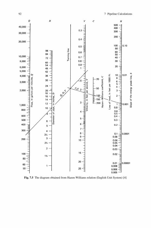
In Fig. 7.5, a diagram that has been made based on Hazen-Williams relationis shown. This diagram is in English units and can be easily used to directly findthe pressure loss in pipes [4]. First, a straight line is drawn between the capacityvalue and the pipe diameter as shown in the figure. This line intersects with theturning line. From the intersection of this line and the turning line, another line isdrawn to connect this point to the value of the Hazen-Williams coefficient, C . Theintersection point of this line and the “loss of head” line will determine the frictionloss per 1000 ft of the pipeline.

As it can be seen, from the figure, this diagram also determines the value of theliquid velocity in the pipe in ft/s. Alternatively, the liquid velocity can be used todetermine the friction loss instead of the flow capacity.

7.3 Pressure Loss in Valves and Other Fittings

The pressure loss in valves, bends, and other fittings in the piping system can bedetermined with two methods that are described in the next two sections.

7.3.1 Equivalent Length Method

In this method, the equivalent length of a straight pipe, corresponding to a specificfitting is determined. When the equivalent length is obtained, it is added to the totalpipe length and the new length is, then, used in calculating the pressure loss in thewhole piping system. The equivalent length of a fitting is the length of a straightpipe that produces the same pressure loss as the fitting.

The diagram presented in Fig. 7.6 can be used to determine the equivalent lengthfor different valves and fittings.

7.3.2 Direct Method

In this method the pressure loss in each fitting in the piping system is obtained fromthe following relation:


Fig. 7.5 The diagram obtained from Hazen-Williams relation (English Unit System) [4]


Fig. 7.6 Determining the equivalent length. First, the pipe diameter is selected from the “InsideDiameter” indicator, right bar. Then, a straight line is drawn from that point to the particular fitting.The intersection of this line with the “equivalent Length Indicator,” second line from the right,would determine the equivalent length, (English Unit System) [5]


Fig. 7.7 Resistance coefficient K for different fittings to be used in (7.15) [6]. D is the pipediameter in inches


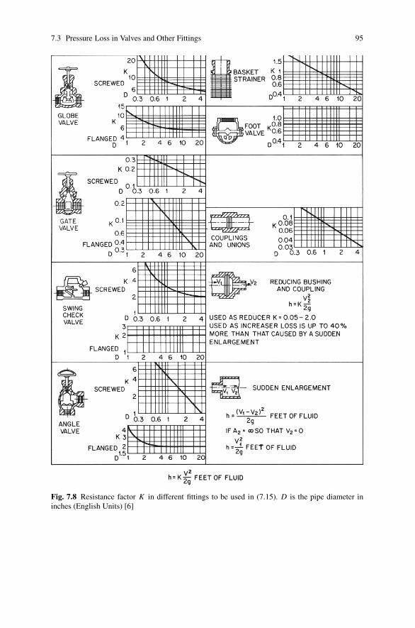
Fig. 7.8 Resistance factor K in different fittings to be used in (7.15). D is the pipe diameter ininches (English Units) [6]


Fig. 7.9 Resistance coefficient K in different fittings. All parameters are defined in the inserts(English Unit System) [6]

HL = KV 2

2g(7.15)

Where K is the resistance coefficients and its value for different fittings has beenpresented in many references. Once K and the flow velocity are known, thepressure loss can be calculated and be added to the pressure loss for straight pipe.Figs. 7.7–7.9 present different K coefficients [6].

For more information about pipeline systems, see [7, 8, 9, 10, 11, 12, 13, 14].

References 97

References

1. “Kubota pump handbook”, Vol. 1, Technical Manual, Kubota Ltd., 1972.2. Karassik Igor J. et al., “Pump Handbook”, McGraw-Hill, 2001.3. “Centrifugal Pump Design”, Technical Appendix, KSB, Frankenthal, Germany.4. Simon Andrew L., “Practical Hydraulics”, John Wiley & Sons, 1981.5. “The Planning of Centrifugal Pumping Plants”, Sulzer Brothers Limited, Pump Division, Win-

ter Thur Switzerland.6. http://www.gouldspumps.com/7. Mohinder L. Nayyar, “Piping Handbook”, 7th ed., McGraw-Hill, New York, 2000.8. Frankel M., “Facility Piping Systems Handbook”, McGraw-Hill, 2002.9. Smith P. “Piping Materials Guide Selection and applications”, Elsevier, 2005.

10. Sanks R. L.,“Pumping Station Design”, Butterworth-Heinemann, 1998.11. Tullis Paul. , “Hydraulics of Pipelines: Pumps, Valves, Cavitation, Transients”, John Wiley &

Sons, 1989.12. Shames I. H. “Mechanics of Fluids”, McGraw-Hill, 1992.13. Streeter V. L., “Fluid Mechanics”, 9th ed., McGraw-Hill, 1997.14. Nourbakhsh S. A., “Pump and Pumping”, University of Tehran Press, 2004.

Pipe Line Calculations

Documents

Transcript of Pipe Line Calculations