Pierre de Fermat (1601 - 1665)

PIERRE DE FERMAT (1601 - 1665)

BEYOND EQUATIONS

Pierre de Fermat (1601 - 1665)

Pierre de Fermat was an amateur mathemati-cian, perhaps the outstanding amateur in the his-tory of mathematics. Born in southwest France,he was home-schooled and then entered the uni-versity in Toulouse, preparing for the life of a civilservant and judge following the wishes of his fam-ily. He rose through the ranks, and became one ofthe most respected jurists in the region.

Fermat did mathematics purely for the love ofit, in the evenings after coming home from work.Unlike Newton, for whom mathematics was pri-marily a means of understanding the natural world,Fermat practiced mathematics for its own sake. His only substantial contribu-tions to physics were in the field of optics, especially Fermat’s Principle, whichis described in this chapter.

Together with Blaise Pascal, Fermat was a founder of probability theory. Heconceived and applied differential calculus years before either Newton or Leibnizwas born, and was also an inventor of analytic geometry. He was a major con-tributor to the theory of numbers, and became most famous for Fermat’s lasttheorem, which states that there are no whole-number solutions (x, y, z) of theequation xn + yn = zn for n an integer, n > 2. Fermat wrote in the margin ofa book: “I have a truly marvelous demonstration of this proposition which thismargin is too narrow to contain.” The attempt to prove the theorem confoundedamateur and professional mathematicians alike for over 300 years, until a proofwas finally constructed by Andrew Weils of Princeton University in 1994, using20th Century mathematics. We may never know for sure whether the very cleverFermat had actually found a proof using mathematics of his day.

Chapter 3

The Variational Principle

While Newton was still a student at Cambridge University, and before hehad discovered his laws of particle motion, Fermat proposed a startlingly dif-ferent explanation of motion. Fermat’s explanation was not for the motion ofparticles, however, but for light rays. In this chapter we explore Fermat’s ap-proach, and then go on to introduce techniques in variational calculus used toimplement this approach, and to solve a number of interesting problems. Wethen show how Einstein’s special relativity and principle of equivalence helpus show how the variational calculus can be used to understand the motionof particles. All this is to set the stage for applying variational techniques togeneral mechanics problems in the following chapter.

3.1 Fermat’s principle

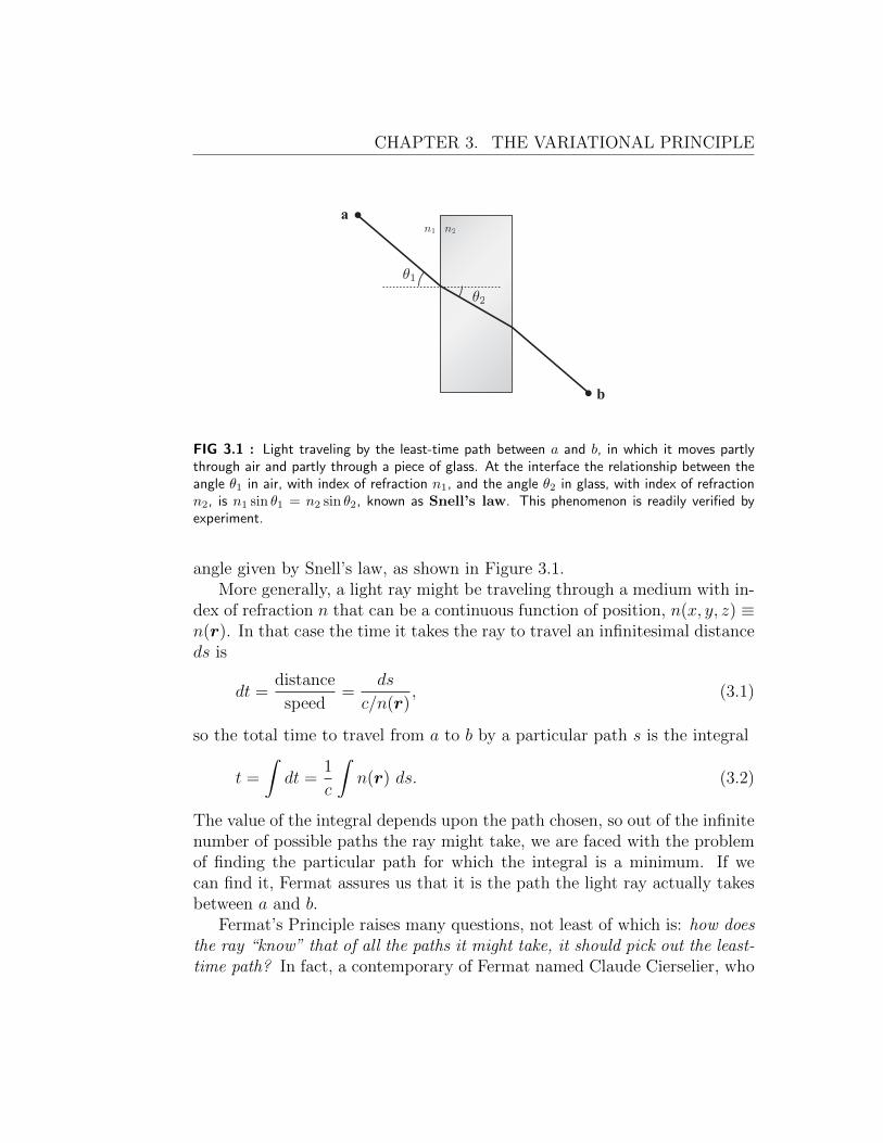
Imagine that a ray of light leaves a light source at point a and travels to someother given point b. Fermat proposed that out of all the infinite number ofpaths that the ray might take between the two points, it actually travels bythe path of least time. For example, if there is nothing but vacuum betweena and b, light traveling at constant speed c takes the path that minimizesthe travel time, which of course is a straight line. Or suppose a piece of glassis inserted into part of an otherwise air-filled space between a and b. In anymedium with index of refraction n, light has speed v = c/n, the minimum-time path in that case is no longer a straight line: Fermat’s principle ofleast time predicts that the ray will bend at the air-glass interface by an

101

CHAPTER 3. THE VARIATIONAL PRINCIPLE

a

b

FIG 3.1 : Light traveling by the least-time path between a and b, in which it moves partlythrough air and partly through a piece of glass. At the interface the relationship between theangle θ1 in air, with index of refraction n1, and the angle θ2 in glass, with index of refractionn2, is n1 sin θ1 = n2 sin θ2, known as Snell’s law. This phenomenon is readily verified byexperiment.

angle given by Snell’s law, as shown in Figure 3.1.More generally, a light ray might be traveling through a medium with in-

dex of refraction n that can be a continuous function of position, n(x, y, z) ≡n(r). In that case the time it takes the ray to travel an infinitesimal distanceds is

dt =distance

speed=

ds

c/n(r), (3.1)

so the total time to travel from a to b by a particular path s is the integral

t =

∫dt =

1

c

∫n(r) ds. (3.2)

The value of the integral depends upon the path chosen, so out of the infinitenumber of possible paths the ray might take, we are faced with the problemof finding the particular path for which the integral is a minimum. If wecan find it, Fermat assures us that it is the path the light ray actually takesbetween a and b.

Fermat’s Principle raises many questions, not least of which is: how doesthe ray “know” that of all the paths it might take, it should pick out the least-time path? In fact, a contemporary of Fermat named Claude Cierselier, who

3.2. THE CALCULUS OF VARIATIONS

was an expert in optics, wrote

. . . Fermat’s principle can not be the cause, for otherwise we would be attributing

knowledge to Nature: and here, by Nature, we understand only that order and

lawfulness in the world, such as it is, which acts without foreknowledge, without

choice, but by a necessary determination.

In Chapter 4.9 we will explain the deep reason why a light ray follows theminimum-time path. But in the meantime we can state that there are sim-ilar minimizing principles for the motion of classical particles, so it will beimportant to understand how to find the path that minimizes some integral,analogous to the integral in (3.2). The technique is called the calculus ofvariations, or functional calculus, and that is the primary topic of thischapter.

3.2 The calculus of variations

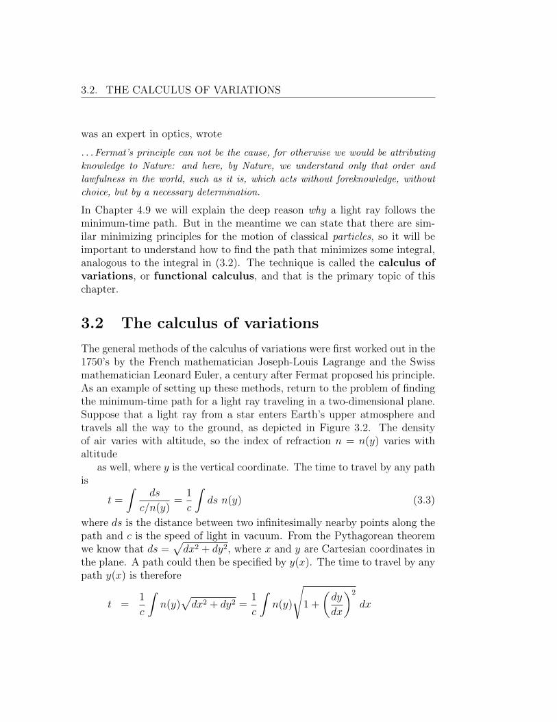
The general methods of the calculus of variations were first worked out in the1750’s by the French mathematician Joseph-Louis Lagrange and the Swissmathematician Leonard Euler, a century after Fermat proposed his principle.As an example of setting up these methods, return to the problem of findingthe minimum-time path for a light ray traveling in a two-dimensional plane.Suppose that a light ray from a star enters Earth’s upper atmosphere andtravels all the way to the ground, as depicted in Figure 3.2. The densityof air varies with altitude, so the index of refraction n = n(y) varies withaltitude

as well, where y is the vertical coordinate. The time to travel by any pathis

t =

∫ds

c/n(y)=

1

c

∫ds n(y) (3.3)

where ds is the distance between two infinitesimally nearby points along thepath and c is the speed of light in vacuum. From the Pythagorean theoremwe know that ds =

√dx2 + dy2, where x and y are Cartesian coordinates in

the plane. A path could then be specified by y(x). The time to travel by anypath y(x) is therefore

t =1

c

∫n(y)

√dx2 + dy2 =

1

c

∫n(y)

√1 +

(dy

dx

)2

dx


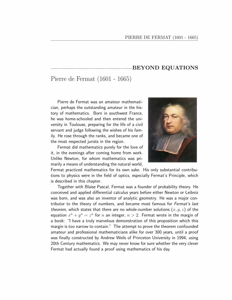
FIG 3.2 : A light ray from a star travels down through Earth’s atmosphere on its way to theground.

≡ 1

c

∫n(y)

√1 + y′2 dx . (3.4)

In this case the integrand depends on both the path y(x) and its slope y′(x).It is easy to imagine that the index of refraction n might also depend upon ahorizontal coordinate x (the density of air might vary somewhat horizontallyas well as vertically), in which case the time for the ray to reach the groundwould be

t =1

c

∫n(x, y)

√1 + y′2 dx ≡

∫F (x, y(x), y′(x)) dx (3.5)

where the integrand F (x, y(x), y′(x)) = (1/c)n(x, y)√

1 + y′2 depends uponall three variables x, y(x), and y′(x). The calculus of variations shows us howto find the particular path y(x) that minimizes this integral.

Finding the least-time path is only one example of a problem in thecalculus of variations. More generally, Euler and Lagrange consider somearbitrary integral I of the form

I =

∫F (x, y(x), y′(x)) dx, (3.6)

and the problem they want to solve is to find not only paths y(x) thatminimize I, but also paths that maximize I, or otherwise make I stationary.


CA

B

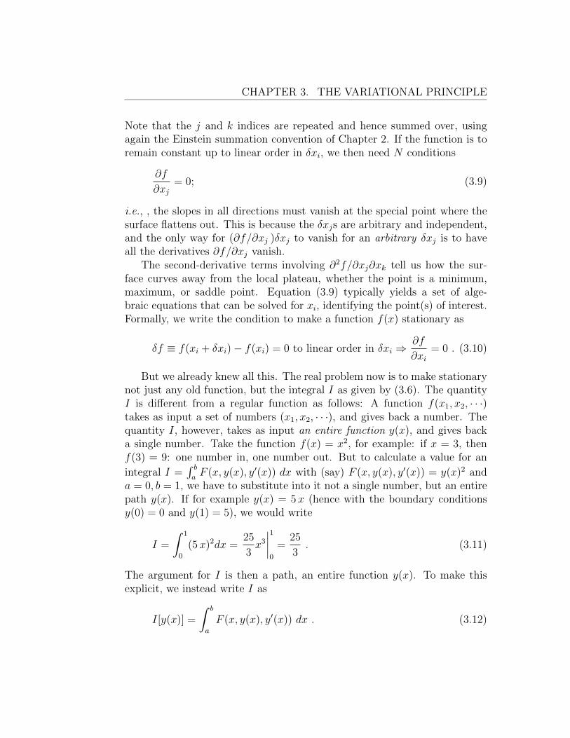
FIG 3.3 : A function of two variables f(x1, x2) with a local minimum at point A, a localmaximum at point B, and a saddle point at C.

It is also possible to have a stationary path that is neither a maximum nora minimum, as we shall see.

How do we go about making I stationary? Let us revisit the more familiarproblem of making an ordinary function stationary. Say we are given afunction f(x1, x2, · · ·) ≡ f(xi) of a number of independent variables xi withi = 1 . . . N , and we are asked to find the stationary points of this function.For the simpler case of a function with only two variables, we can visualize theproblem as shown in Figure 3.3: we have a curved surface f(x1, x2) over thex1-x2 plane, and we are looking for special points (x1, x2) where the surfaceis “locally flat”. These can correspond to minima, maxima, or saddle points,as shown in the figure. Algebraically, we can phrase the general problemas follows. For every point (x1, x2, · · ·), we move away by a small arbitrarydistance δxi

xi → xi + δxi . (3.7)

We then seek a special point (x1, x2, · · ·) where this shift does not changethe function f(xi) to linear order in the small shifts δxi. This is to be ourintuitive meaning of being ‘locally flat’. Using a Taylor expansion, we canthen write

f(xi)→ f(xi + δxi) = f(xi) +∂f

∂xjδxj +

1

2!

∂2f

∂xjxkδxjδxk + · · · (3.8)


Note that the j and k indices are repeated and hence summed over, usingagain the Einstein summation convention of Chapter 2. If the function is toremain constant up to linear order in δxi, we then need N conditions

∂f

∂xj= 0; (3.9)

i.e., , the slopes in all directions must vanish at the special point where thesurface flattens out. This is because the δxjs are arbitrary and independent,and the only way for (∂f/∂xj )δxj to vanish for an arbitrary δxj is to haveall the derivatives ∂f/∂xj vanish.

The second-derivative terms involving ∂2f/∂xj∂xk tell us how the sur-face curves away from the local plateau, whether the point is a minimum,maximum, or saddle point. Equation (3.9) typically yields a set of alge-braic equations that can be solved for xi, identifying the point(s) of interest.Formally, we write the condition to make a function f(x) stationary as

δf ≡ f(xi + δxi)− f(xi) = 0 to linear order in δxi ⇒∂f

∂xi= 0 . (3.10)

But we already knew all this. The real problem now is to make stationarynot just any old function, but the integral I as given by (3.6). The quantityI is different from a regular function as follows: A function f(x1, x2, · · ·)takes as input a set of numbers (x1, x2, · · ·), and gives back a number. Thequantity I, however, takes as input an entire function y(x), and gives backa single number. Take the function f(x) = x2, for example: if x = 3, thenf(3) = 9: one number in, one number out. But to calculate a value for an

integral I =∫ baF (x, y(x), y′(x)) dx with (say) F (x, y(x), y′(x)) = y(x)2 and

a = 0, b = 1, we have to substitute into it not a single number, but an entirepath y(x). If for example y(x) = 5x (hence with the boundary conditionsy(0) = 0 and y(1) = 5), we would write

I =

∫ 1

0

(5x)2dx =25

3x3

∣∣∣∣10

=25

3. (3.11)

The argument for I is then a path, an entire function y(x). To make thisexplicit, we instead write I as

I[y(x)] =

∫ b

a

F (x, y(x), y′(x)) dx . (3.12)


FIG 3.4 : Various paths y(x) that can be used as input to the functional I[f(x)]. We lookfor that special path from which an arbitrary small displacement δy(x) leaves the functionalunchanged to linear order in δy(x). Note that δy(a) = δy(b) = 0.

with square brackets around the argument: I is not a function, but is calleda functional.

In general, a functional may take as argument several functions, not justone. But for now let us focus on the case of a functional depending on a singlefunction. The question we want to address is then: how do we make such afunctional stationary? This means we are looking for conditions that identifya set of paths y(x) where the functional I[y(x)] is stationary or ‘locally flat’.To do this, we can build upon the simpler example of making stationary afunction. For any path y(x), we look at a shifted path

y(x)→ y(x) + δy(x) (3.13)

where δy(x) is a function that is small everywhere, but is otherwise arbitrary.However, we require that at the endpoints of the integration in (3.12), theshifts vanish; i.e., , δy(a) = δy(b) = 0. This means that we do not perturbthe boundary conditions on trial paths that are fed into I[y(x)], because weonly need to find the path that makes stationary the functional amongst thesubset of all possible paths that satisfy the given fixed boundary conditionsat the endpoints. We illustrate this in Figure 3.4. In this restricted setof trial paths, our functional extremization condition now looks very muchlike (3.10)

δI[y(x)] ≡ I[y(x) + δy(x)]− I[y(x)] = 0 (3.14)


FIG 3.5 : A discretization of a path.

to linear order in δy(x). We say: “the variation of the functional I is zero.”For a function f(x1, x2, · · ·), the condition amounted to setting all first deriva-tives of f to zero. Hence, we need to figure out how to differentiate a func-tional! Alternatively, we need to expand the functional I[y(x) + δy(x)] inδy(x) to linear order to identify its ‘first derivative’.

Fortunately, we can deduce all operations of functional calculus by think-ing of a functional in the following way. Imagine that the input to thefunctional, the path y(x), is evaluated only on a finite discrete set of points:

a < x < b→ x = a+ n ε ≤ b (3.15)

for n a non-negative integer and ε small (see Figure 3.5).In the limit ε → 0 and n →∞, we recover the original continuum prob-

lem. The functional is now simply a function of a finite number of variablesy(a), y(a + ε), y(a + 2 ε), · · ·. In the limit ε → 0, the set becomes infinitelydense. You can hence view a functional as a function of an infinite numberof variables. We can perform all needed operations on I in the discretizedregime where I is treated as a function; and then take the ε→ 0 limit at theend of the day.

Basically, we may think of x in y(x) as a discrete index yx. We thenhave I[y(x)] → I(yx), a function with a large but finite number of variablesyx, with x ∈ {a · · · b} a finite set. A functional then becomes a much morefamiliar animal: a function. The integral I may also depend upon y′(x),


which can be written in our discrete way as y′(x) → (yx − yx−ε)/ε by thedefinition of the derivative operation. We write it in shorthand as y′(x)→ y′x;and the integration in (3.12) becomes a sum:

∫dx →

∑x ε. To summarize,

we now have a discretized form of our original functional

I =∑x

F (x, yx, y′x) ε . (3.16)

We can now apply the shifts yx → yx + δyx, which also implies y′x →y′x + δy′x, where δy′x = (δyx − (δy)x−ε)/ε = d(δyx)/dx. We then need theanalogue to

δf =∂f

∂xiδxi = 0 (3.17)

with f → I, and xi → yx. Starting from (3.16), we have

δI =∑x

(∂F

∂yxδyx +

∂F

∂y′xδy′x

)ε = 0 . (3.18)

In the ε→ 0 limit we retrieve the integral form

δI[y(x)] =

∫ b

a

(∂F

∂y(x)δy(x) +

∂F

∂y′(x)

d

dx(δy(x))

)dx = 0. (3.19)

Integrating the second term by parts, we get∫ b

a

∂F

∂y′(x)

d

dx(δy(x)) = δy(x)

∂F

∂y′(x)

∣∣∣∣ba

−∫ b

a

δy(x)d

dx

(∂F

∂y′(x)

)dx(3.20)

where the first term on the right vanishes because we have fixed the endpointsso that δy(a) = δy(b) = 0. Therefore equation (3.19) becomes

δI[y(x)] =

∫ b

a

(∂F

∂y(x)− d

dx

(∂F

∂y′(x)

))δy(x) dx = 0. (3.21)

This integral might be zero because the integrand is zero for all x, or be-cause there are positive and negative portions that cancel one another out.However, since arbitrary smooth deviation functions δy(x) are permitted, thefirst alternative has to be the right one. For example, if a < x0 < b and theintegrand happens to be positive from a to x0 and negative from x0 to b sothat by cancellation the overall integral is zero, the deviation function δy(x)


could be changed so that δy(x) = 0 from x0 to b, which would force theintegral to be positive. Therefore the requirement that the integral vanishfor arbitrary smooth functions δy(x) requires that

∂F

∂y(x)− d

dx

(∂F

∂y′(x)

)= 0 , (3.22)

which is known as Euler’s equation. This equation was worked out byboth Euler and Lagrange about the same time, but we will call it simply“Euler’s equation”, because we will reserve the term “Lagrange equations”for essentially the same equation when used in classical mechanics, as we willsee in Chapter 4.

Note two important features of Euler’s equation:

1. The derivatives with respect to y and y′ are partial, but the derivativewith respect to x is total. Suppose, for example, that F (x, y(x), y′(x)) =x y (y′)2. Then ∂F/∂y = (y′)2 x and ∂F/∂y′ = 2x y y′, so Euler’s equa-tion becomes

x (y′)2− d

dx(2x y y′) = x (y′)2−[2 y y′+2x (y′)2+2x y y′′] = 0.(3.23)

This is an ordinary differential equation whose solution y(x) is thepath we are looking for. That is, in the calculus of variations, Euler’sequation converts the problem of finding which path makes a particu-lar integral stationary into a differential equation for the path, whosesolution gives the path we want.

2. The variables x and y in Euler’s equation do not have to representCartesian coordinates. The mathematics has no idea what x and yrepresent, as long as they are independent of one another. So if anintegral I has the form of (3.12), but with x and y replaced by differ-ent symbols, the corresponding Euler’s equation still holds. The totalderivative occurring in the equation is always with respect to whatevervariable of integration is chosen in the problem, which is called the in-dependent variable. For example, if the integral to be made stationaryhas the form

I[q(t)] =

∫F (t, q(t), q′(t))dt (3.24)

3.3. GEODESICS

then the corresponding Euler equation is

∂F

∂q(t)− d

dt

(∂F

∂q′(t)

)= 0. (3.25)

t is then the independent variable while q(t) is referred to as the de-pendent variable; and q′(t) ≡ dq/dt.

3.3 Geodesics

The calculus of variations is best learned through examples. Let us proceedto a sequence of explicit cases where these techniques can come in handy.One application is to find geodesics, which are the stationary (usually theshortest) paths between two points on a given surface.

EXAMPLE 3-1: Geodesics on a plane

We have in effect already set up the problem of finding the geodesic paths on a plane.The appropriate integral in that case is

s =

∫ √dx2 + dy2 =

∫ b

a

√1 +

(dy

dx

)2

dx ≡∫ b

a

√1 + y′2 dx. (3.26)

We then have F =√

1 + y′2 in equation (3.6)). Note that the integrand does not dependupon either x or y(x) explicitly, so ∂F/∂y = 0. Euler’s equation (3.22 then becomes simply

d

dx

(∂F

∂y′

)= 0 (3.27)

and so

∂F

∂y′=

y′√1 + (y′)2

= k, (3.28)

where k is a constant. Solving for y′,

y′ =±k√

1− k2≡ m1, (3.29)

which defines the constant m1 in terms of the constant k. The integral of this equation isy = m1 x + m2, where m2 is a constant of integration. That is, the shortest distance on a


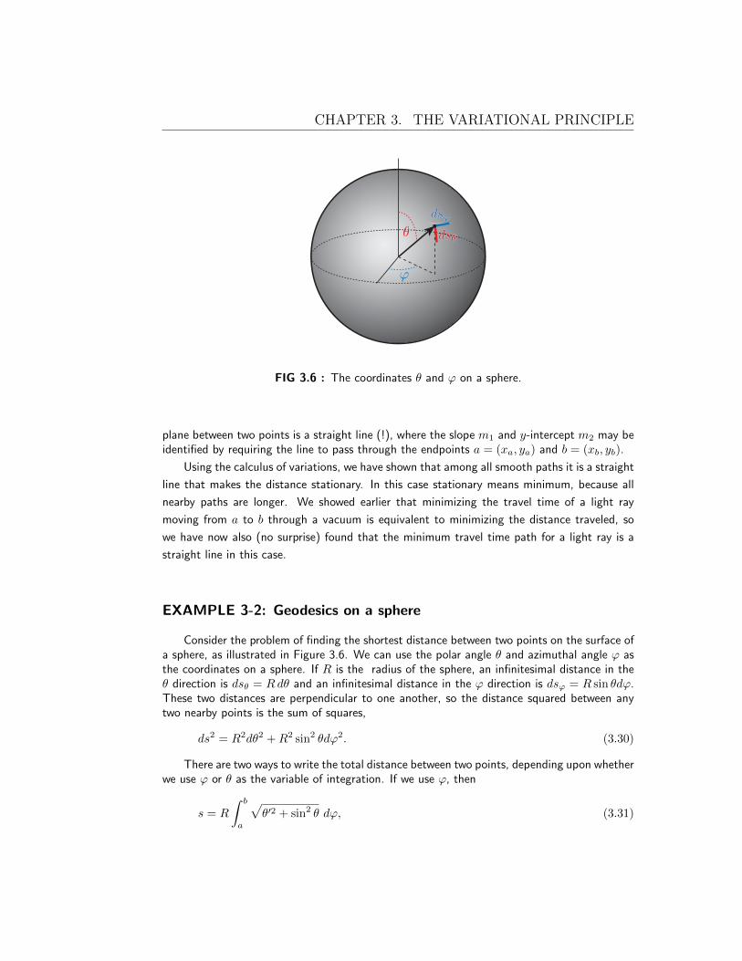
FIG 3.6 : The coordinates θ and ϕ on a sphere.

plane between two points is a straight line (!), where the slope m1 and y-intercept m2 may beidentified by requiring the line to pass through the endpoints a = (xa, ya) and b = (xb, yb).

Using the calculus of variations, we have shown that among all smooth paths it is a straight

line that makes the distance stationary. In this case stationary means minimum, because all

nearby paths are longer. We showed earlier that minimizing the travel time of a light ray

moving from a to b through a vacuum is equivalent to minimizing the distance traveled, so

we have now also (no surprise) found that the minimum travel time path for a light ray is a

straight line in this case.

EXAMPLE 3-2: Geodesics on a sphere

Consider the problem of finding the shortest distance between two points on the surface ofa sphere, as illustrated in Figure 3.6. We can use the polar angle θ and azimuthal angle ϕ asthe coordinates on a sphere. If R is the radius of the sphere, an infinitesimal distance in theθ direction is dsθ = Rdθ and an infinitesimal distance in the ϕ direction is dsϕ = R sin θdϕ.These two distances are perpendicular to one another, so the distance squared between anytwo nearby points is the sum of squares,

ds2 = R2dθ2 +R2 sin2 θdϕ2. (3.30)

There are two ways to write the total distance between two points, depending upon whetherwe use ϕ or θ as the variable of integration. If we use ϕ, then

s = R

∫ b

a

√θ′2 + sin2 θ dϕ, (3.31)

3.3. GEODESICS

where θ′ = dθ/dϕ. The corresponding Euler equation is

∂F

∂θ− d

dϕ

∂F

∂θ′= 0 (3.32)

where F =√θ′2 + sin2 θ. Alternatively, we can write

s = R

∫ b

a

√1 + sin2 θ ϕ′2 dθ, (3.33)

where ϕ′ = dϕ/dθ with the corresponding Euler equation

∂F

∂ϕ− d

dθ

∂F

∂ϕ′= 0, (3.34)

and where in this case F =√

1 + sin2 θ ϕ′2. Both Euler equations are correct. Is one easierto use than the other?

In the first alternative, equation (3.32)) results in a second-order differential equation,since the first term ∂F/∂θ 6= 0 and by the time all the derivatives are taken the second termincludes a second derivative θ′′. The second alternative (3.34 is much easier to use, because

in that case F =√

1 + sin2 θ ϕ′2 is not an explicit function of ϕ, so the first term in Euler’sequation vanishes. The quantity ∂F/∂ϕ′ must therefore be constant in θ, since its totalderivative is zero. This leaves us with only a first-order differential equation

∂F

∂ϕ′=

sin2 θ ϕ′√1 + sin2 θϕ′2

= k, (3.35)

for some constant k, which can be solved for ϕ′ and rearranged to give

ϕ′ = ± k csc2 θ√1− k2 csc2 θ

. (3.36)

Using the identity csc2 θ = 1 + cot2 θ and substituting q = α cot θ, where α = k/√

1− k2,gives

ϕ = α

∫dq√

1− q2= α sin−1 q + β, (3.37)

where α = ±(√

1− k2)/k and β is a constant of integration. Therefore the equation relatingθ and ϕ is

sin(ϕ− β) = q = α cot θ. (3.38)

We can better understand the meaning of this result by multiplying through by R cos θ andusing the identity sin(ϕ− β) = sinϕ cosβ − cosϕ sinβ, which gives

(cosβ)y − (sinβ)x = αz (3.39)


(a) (b)

FIG 3.7 : (a) Great circles on a sphere are geodesics; (b) Two paths nearby the longer of thetwo great-circle routes of a path.

where x = R sin θ cosϕ, y = R sin θ sinϕ, and z = R cos θ, which are the Cartesian coordi-nates on the sphere. Equation (3.39) is the equation of a plane passing through the centerof the sphere, which slices through the sphere in a great circle. So we have found that thesolutions of Euler’s equation are great-circle routes, as illustrated in 3.7(a).

Unless one endpoint is at the antipode of the other, there is a shorter distance and a longer

distance along the great circle that connects them. The shorter distance is a minimum path

length under small deviations in path, as is well known by airline pilots. The larger distance is

a stationary path that is neither a minimum nor a maximum under all small deviations in path.

Paths that oscillate around this path are generally longer than the great-circle route, while

some paths pulled to one side of the great-circle route are shorter. Both kinds are sketched

in 3.7(b). This behavior is fairly typical of stationary paths that are neither absolute maxima

nor absolute minima relative to all neighboring paths: Some neighboring paths lead to smaller

values and others lead to larger values of the integral I. In this case the set of all such paths

represent a kind of saddle in a very large-dimensional space.

3.4 Brachistochrone

The brachistochrone (“shortest time”) problem was invented and solved ahalf century before the work of Euler and Lagrange, and engaged some of themost creative people in the history of physics and mathematics. The problemis to find the shape of a frictionless track between two given points, such thata small block starting at rest at the upper point — and sliding without friction

3.4. BRACHISTOCHRONE

a

b

Curve 3Curve 2Curve 1

Curve 4

FIG 3.8 : Possible least-time paths for a sliding block.

down along the track under the influence of gravity — arrives at the lowerpoint in the shortest time. The two points a and b, and shapes of possibletracks between them, are illustrated in 3.8.

We can guess the qualitative shape of the shortest-time track by physicalreasoning. Of the four curves shown in Figure 3.8, it might seem that thestraight line 3 is the shortest-time path, since it is the path of shortest dis-tance. However, curve 2 has an advantage in that the block picks up speedmore quickly, so that its greater average speed may more than make up forthe greater distance it has to travel. Curve 1 permits the block to pick upspeed still faster, but there is a risk that the slightly increased average speedmight not outweigh the greater distance involved. There is no reason tochoose curve 4, because a block will hardly get going in the first place and italso has to travel relatively far. A track whose shape is something like curve2 should be the best choice.

To find the exact shape we choose coordinates as shown in Figure 3.8,with the origin at the release point, the positive y axis extending downward,and the final point designated by (xb, yb). The time to travel over a shortdistance is the distance divided by the speed, so the overall time is

t =

∫ds

v(3.40)

where v is the varying speed of the block. The infinitesimal distance is againds =

√dx2 + dy2. Since v changes in general along the track, we need to


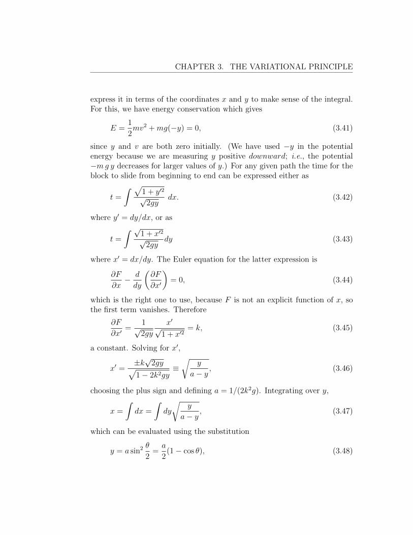
express it in terms of the coordinates x and y to make sense of the integral.For this, we have energy conservation which gives

E =1

2mv2 +mg(−y) = 0, (3.41)

since y and v are both zero initially. (We have used −y in the potentialenergy because we are measuring y positive downward; i.e., the potential−mg y decreases for larger values of y.) For any given path the time for theblock to slide from beginning to end can be expressed either as

t =

∫ √1 + y′2√

2gydx. (3.42)

where y′ = dy/dx, or as

t =

∫ √1 + x′2√

2gydy (3.43)

where x′ = dx/dy. The Euler equation for the latter expression is

∂F

∂x− d

dy

(∂F

∂x′

)= 0, (3.44)

which is the right one to use, because F is not an explicit function of x, sothe first term vanishes. Therefore

∂F

∂x′=

1√2gy

x′√1 + x′2

= k, (3.45)

a constant. Solving for x′,

x′ =±k√

2gy√1− 2k2gy

≡√

y

a− y, (3.46)

choosing the plus sign and defining a = 1/(2k2g). Integrating over y,

x =

∫dx =

∫dy

√y

a− y, (3.47)

which can be evaluated using the substitution

y = a sin2 θ

2=a

2(1− cos θ), (3.48)


a

b1 b2

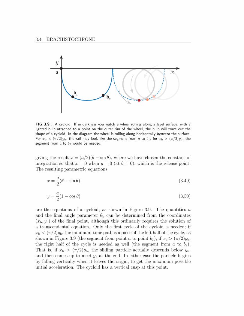
FIG 3.9 : A cycloid. If in darkness you watch a wheel rolling along a level surface, with alighted bulb attached to a point on the outer rim of the wheel, the bulb will trace out theshape of a cycloid. In the diagram the wheel is rolling along horizontally beneath the surface.For xb < (π/2)yb, the rail may look like the segment from a to b1; for xb > (π/2)yb, thesegment from a to b2 would be needed.

giving the result x = (a/2)(θ − sin θ), where we have chosen the constant ofintegration so that x = 0 when y = 0 (at θ = 0), which is the release point.The resulting parametric equations

x =a

2(θ − sin θ) (3.49)

y =a

2(1− cos θ) (3.50)

are the equations of a cycloid, as shown in Figure 3.9. The quantities aand the final angle parameter θb can be determined from the coordinates(xb, yb) of the final point, although this ordinarily requires the solution ofa transcendental equation. Only the first cycle of the cycloid is needed; ifxb < (π/2)yb, the minimum-time path is a piece of the left half of the cycle, asshown in Figure 3.9 (the segment from point a to point b1); if xb > (π/2)yb,the right half of the cycle is needed as well (the segment from a to b2).That is, if xb > (π/2)yb, the sliding particle actually descends below yb,and then comes up to meet yb at the end. In either case the particle beginsby falling vertically when it leaves the origin, to get the maximum possibleinitial acceleration. The cycloid has a vertical cusp at this point.


The time required to fall to the final point can be found by returningto equation (3.43)) and expressing x and y in terms of the parameter θ,according to equations (3.49) and (3.50. The result is simply

t =

√a

2g

∫ θf

0

dθ =

√a

2gθf . (3.51)

In particular, if (xb, yb) = (πa/2, a), so that a complete half-cycle of thecycloid is needed to connect the points, then θf = π and

t = π

√a

2g. (3.52)

This is the time it would take a particle to slide from the rim to the bottomof a smooth cycloidal bowl, where a is the depth of the bowl.1

EXAMPLE 3-3: Fermat again

1A bit of history: On the afternoon of January 29, 1697, Sir Isaac Newton, who hadleft Cambridge the previous year to become Warden of the Mint in London, returned tohis London home from a hard day at the Mint to find a letter from the Swiss mathemati-cian Johann Bernoulli. The letter contained the brachistochrone problem, published theprevious June. A challenge had gone forth to mathematicians to solve the problem, andthey were given a time limit of six months to find the solution. Gottfried Wilhelm Leibniz,German mathematician and arch rival of Newton for recognition as the original inventorof calculus, solved the problem but asked that the deadline be extended by an additionalyear so that everyone would have a chance to try it. Bernoulli agreed. Although presentedas a general challenge, Bernoulli specifically sent the problem to Newton, who had notseen it before, to alert him to the problem and to try to stump him, thereby showing thathe did not really understand calculus as well as the continental mathematicians.

Newton’s niece, Catherine Barton, was living with him in London at the time. Shelater testified that “Sr I. N. was in the midst of the hurry of the great recoinage anddid not come home till four from the Tower very much tired, but did not sleep till hehad solved it wch was by 4 in the morning.” Newton sent off the solution that samemorning to the Royal Society, and it was published anonymously in the February issue ofthe Philosophical Transactions. Bernoulli had no doubt who was responsible, and wroteto a friend that it was “ex ungue Leonum” — “from the claws of the Lion.” Aside fromNewton, Leibniz, and Johann Bernoulli himself, the brachistochrone problem was solvedby only two other mathematicians at that time, Bernoulli’s older brother Jacob and theFrench mathematician de l’Hospital. All of the solutions were ad hoc, involving algorithmssuited to the particular problem, but not necessarily easily generalizable to a wider classof problems.


(a) (b)

1

2

3

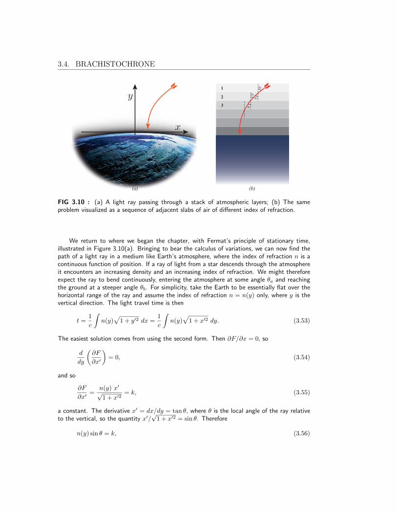
FIG 3.10 : (a) A light ray passing through a stack of atmospheric layers; (b) The sameproblem visualized as a sequence of adjacent slabs of air of different index of refraction.

We return to where we began the chapter, with Fermat’s principle of stationary time,illustrated in Figure 3.10(a). Bringing to bear the calculus of variations, we can now find thepath of a light ray in a medium like Earth’s atmosphere, where the index of refraction n is acontinuous function of position. If a ray of light from a star descends through the atmosphereit encounters an increasing density and an increasing index of refraction. We might thereforeexpect the ray to bend continuously, entering the atmosphere at some angle θa and reachingthe ground at a steeper angle θb. For simplicity, take the Earth to be essentially flat over thehorizontal range of the ray and assume the index of refraction n = n(y) only, where y is thevertical direction. The light travel time is then

t =1

c

∫n(y)

√1 + y′2 dx =

1

c

∫n(y)

√1 + x′2 dy. (3.53)

The easiest solution comes from using the second form. Then ∂F/∂x = 0, so

d

dy

(∂F

∂x′

)= 0, (3.54)

and so

∂F

∂x′=

n(y) x′√1 + x′2

= k, (3.55)

a constant. The derivative x′ = dx/dy = tan θ, where θ is the local angle of the ray relativeto the vertical, so the quantity x′/

√1 + x′2 = sin θ. Therefore

n(y) sin θ = k, (3.56)


a constant everywhere along the path. This result could also have been obtained immediatelyfrom Snell’s law, by modeling the atmosphere as a large number of thin horizontal layers, wheren is constant within each layer, but with n increasing slightly as one passes from one layer to thelayer just beneath it. Snell’s law is obeyed at each boundary: for example, n1 sin θ1 = n2 sin θ2

as shown in Figure 3.1. However, the angle θ2 at which the ray leaves layer 2 is the same angleat which the ray leaves layer 2 at the boundary with layer 3 (see Figure 3.10(b)). Thereforealso n2 sin θ2 = n3 sin θ3 , etc., so in the stack of layers it follows that n(y) sin θ = constant.In the limit where the stack approaches an infinite number of layers of infinitesimal thickness,we get equation (3.56). Given a function n(y) we can then find the specific path shape y(x)from θ(y) (See problems at the end of the chapter.)

Note that the constancy of n sin θ allows us to predict the ray angle θb at the groundwithout knowing the detailed index of refraction n(y) or the path of the ray! If we know theindices of refraction at the top of the atmosphere na and at the ground nb, and the angle atwhich the ray enters the atmosphere θa (from the true location of the star) we can find theangle at the ground θb — which is the angle at which a telescope would observe the star — as

na sin θa = nb sin θb = constant (3.57)

3.5 Several Dependent Variables

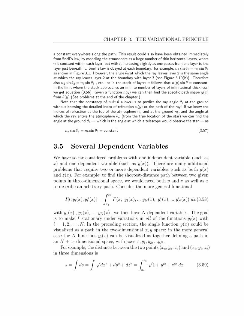
We have so far considered problems with one independent variable (such asx) and one dependent variable (such as y(x)). There are many additionalproblems that require two or more dependent variables, such as both y(x)and z(x). For example, to find the shortest-distance path between two givenpoints in three-dimensional space, we would need both y and z as well as xto describe an arbitrary path. Consider the more general functional

I[t, yi(x), yi′(x)] =

∫ x2

x1

F (x, y1(x), ... yN(x), y′1(x), ... y′N(x)) dx(3.58)

with y1(x) , y2(x), ..., yN(x) , we then have N dependent variables. The goalis to make I stationary under variations in all of the functions yi(x) withi = 1, 2, . . . , N. In the preceding section, the single function y(x) could bevisualized as a path in the two-dimensional x, y space; in the more generalcase the N functions yi(x) can be visualized as together defining a path inan N + 1- dimensional space, with axes x, y1, y2, ...yN .

For example, the distance between the two points (xa, ya, za) and (xb, yb, zb)in three dimensions is

s =

∫ds =

∫ √dx2 + dy2 + dz2 =

∫ xb

xa

√1 + y′2 + z′2 dx (3.59)

3.5. SEVERAL DEPENDENT VARIABLES

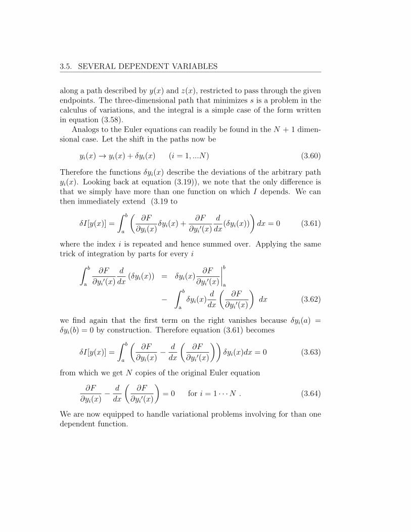
along a path described by y(x) and z(x), restricted to pass through the givenendpoints. The three-dimensional path that minimizes s is a problem in thecalculus of variations, and the integral is a simple case of the form writtenin equation (3.58).

Analogs to the Euler equations can readily be found in the N + 1 dimen-sional case. Let the shift in the paths now be

yi(x)→ yi(x) + δyi(x) (i = 1, ...N) (3.60)

Therefore the functions δyi(x) describe the deviations of the arbitrary pathyi(x). Looking back at equation (3.19)), we note that the only difference isthat we simply have more than one function on which I depends. We canthen immediately extend (3.19 to

δI[y(x)] =

∫ b

a

(∂F

∂yi(x)δyi(x) +

∂F

∂yi′(x)

d

dx(δyi(x))

)dx = 0 (3.61)

where the index i is repeated and hence summed over. Applying the sametrick of integration by parts for every i∫ b

a

∂F

∂yi′(x)

d

dx(δyi(x)) = δyi(x)

∂F

∂yi′(x)

∣∣∣∣ba

−∫ b

a

δyi(x)d

dx

(∂F

∂yi′(x)

)dx (3.62)

we find again that the first term on the right vanishes because δyi(a) =δyi(b) = 0 by construction. Therefore equation (3.61) becomes

δI[y(x)] =

∫ b

a

(∂F

∂yi(x)− d

dx

(∂F

∂yi′(x)

))δyi(x)dx = 0 (3.63)

from which we get N copies of the original Euler equation

∂F

∂yi(x)− d

dx

(∂F

∂yi′(x)

)= 0 for i = 1 · · ·N . (3.64)

We are now equipped to handle variational problems involving for than onedependent function.


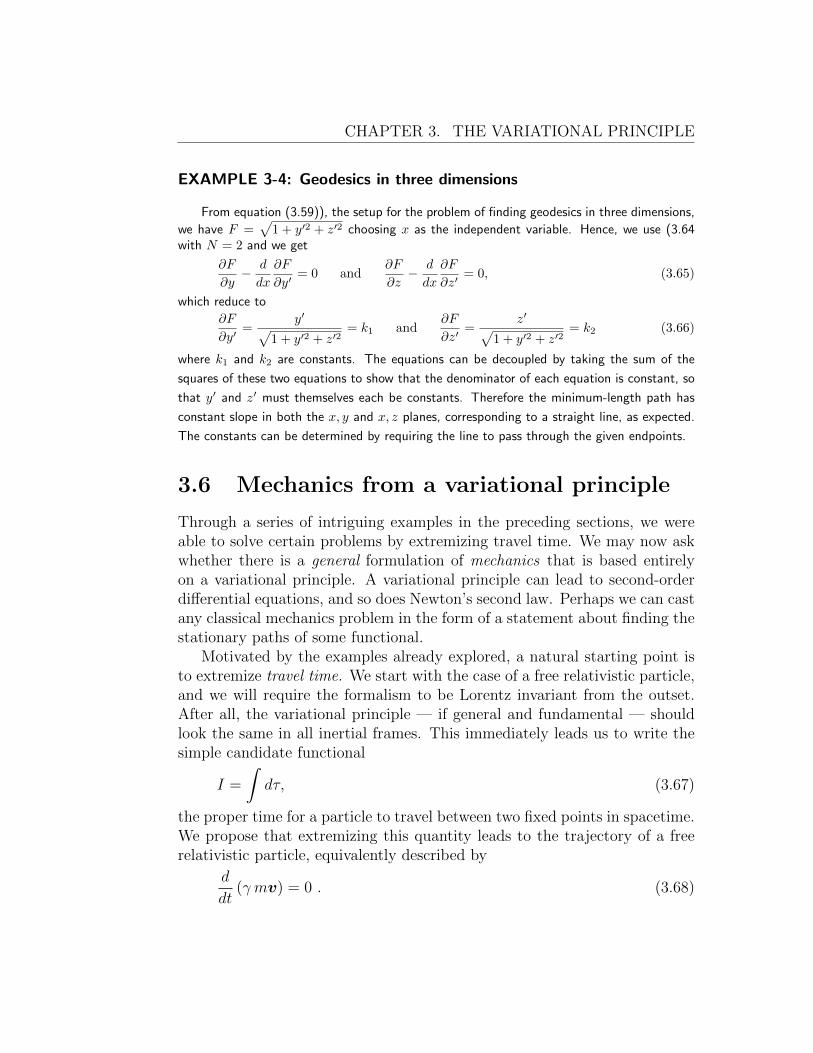
EXAMPLE 3-4: Geodesics in three dimensions

From equation (3.59)), the setup for the problem of finding geodesics in three dimensions,

we have F =√

1 + y′2 + z′2 choosing x as the independent variable. Hence, we use (3.64with N = 2 and we get

∂F

∂y− d

dx

∂F

∂y′= 0 and

∂F

∂z− d

dx

∂F

∂z′= 0, (3.65)

which reduce to

∂F

∂y′=

y′√1 + y′2 + z′2

= k1 and∂F

∂z′=

z′√1 + y′2 + z′2

= k2 (3.66)

where k1 and k2 are constants. The equations can be decoupled by taking the sum of the

squares of these two equations to show that the denominator of each equation is constant, so

that y′ and z′ must themselves each be constants. Therefore the minimum-length path has

constant slope in both the x, y and x, z planes, corresponding to a straight line, as expected.

The constants can be determined by requiring the line to pass through the given endpoints.

3.6 Mechanics from a variational principle

Through a series of intriguing examples in the preceding sections, we wereable to solve certain problems by extremizing travel time. We may now askwhether there is a general formulation of mechanics that is based entirelyon a variational principle. A variational principle can lead to second-orderdifferential equations, and so does Newton’s second law. Perhaps we can castany classical mechanics problem in the form of a statement about finding thestationary paths of some functional.

Motivated by the examples already explored, a natural starting point isto extremize travel time. We start with the case of a free relativistic particle,and we will require the formalism to be Lorentz invariant from the outset.After all, the variational principle — if general and fundamental — shouldlook the same in all inertial frames. This immediately leads us to write thesimple candidate functional

I =

∫dτ, (3.67)

the proper time for a particle to travel between two fixed points in spacetime.We propose that extremizing this quantity leads to the trajectory of a freerelativistic particle, equivalently described by

d

dt(γ mv) = 0 . (3.68)

3.6. MECHANICS FROM A VARIATIONAL PRINCIPLE

from (2.100). Armed with the techniques developed in the previous sections,we can check whether this statement is correct.

We write the functional in terms of the coordinate system of some inertialobserver O using coordinates (c t, x, y, z)

I =

∫dτ =

∫dt

γ=

∫dt

√1− x2 + y2 + z2

c2(3.69)

where we used the time dilation relation dt = γ dτ . We need to determinethree functions x(t), y(t), and z(t) that extremize the functional I whoseindependent variable is t. We can imagine that the endpoints of the trajectoryare fixed, and so we have a familiar variational problem. We can then useEuler’s equations (3.64) with

F =

√1− x2

c2− y2

c2− z2

c2. (3.70)

and N = 3. We have three equations

∂F

∂x− d

dt

∂F

∂x= 0 ,

∂F

∂y− d

dt

∂F

∂y= 0 ,

∂F

∂z− d

dt

∂F

∂z= 0 . (3.71)

It is straightforward to show that these lead to

d

dt(γx) = 0 ,

d

dt(γy) = 0 ,

d

dt(γz) = 0 ; (3.72)

That is, equation (3.68). This is already very promising: we can describe afree relativistic particle by extremizing the particle’s proper time.

Let us next look at the low-velocity regime of our functional. We write (3.69)in an expanded form for β � 1

I '∫dt

(1− 1

2

v2

c2+ · · ·

). (3.73)

The first term is a constant and does not affect a variational principle: Euler’sequations involve derivatives of F and hence constant terms in F may safelybe dropped. The second term is quadratic in the velocity. We rewrite ourfunctional as

I →∫dt

(1

2m(x2 + y2 + z2

)). (3.74)


In addition to dropping the constant shift term, we have also multiplied Ifrom (3.73)) by −mc2 for convenience. This is a multiplication by a constantand hence, once again, does not affect the Euler equations (3.64). It makesthings a little more suggestive, however: we are now extremizing the particle’snon-relativistic kinetic energy. If we now use Euler’s equations (3.64 withF = (1/2)mv2, we get the familiar three differential equations

d

dt(mv) = 0 , (3.75)

as expected. So far so good. We have the expected results for free particles!But how about problems that involve forces?

3.7 Motion in a uniform gravitational field

Shortly after developing his special theory of relativity, Einstein saw a beau-tiful way to understand the effect of uniform gravitational forces, which hecalled the principle of equivalence. He later said that it was “the happiestthought of my life”, because it was a wonderfully simple but powerful ideathat became a crucial steppingstone to achieving his relativistic theory ofgravity: general relativity.

The equivalence principle can be illustrated by experiments carried out intwo spaceships, one accelerating uniformly in gravity-free empty space andone standing at rest in a uniform gravitational field, as shown in Figure 3.11.The acceleration a of the first ship is numerically equal, but opposite indirection, to the gravitational field g acting on the second ship. The equiva-lence principle then claims that if observers in either one of the ships carryout any experiment whatever that is confined entirely within their own ship,the results cannot be used to determine which ship they are living in: thetwo situations are equivalent. This is a statement inspired by observation —dating back to Galileo’s Pisa tower experiment equating inertial and gravi-tational masses — which Einstein then elevated to the stature of a principleof Nature.

We use the principle here to deduce two related effects of gravity that arenot contained in Newton’s theory: the gravitational frequency shift and theeffect of gravity on the rate of clocks. We start by considering a particularthought experiment with light waves. An observer in the bow of the acceler-ating ship shines a laser beam at another observer in the stern of the ship,

3.7. MOTION IN A UNIFORM GRAVITATIONAL FIELD

(a) (b)

a

FIG 3.11 : Two spaceships, one accelerating in gravity-free space (a), and the other at reston the ground (b). Neither observers in the accelerating ship nor those in the ship at rest onthe ground can find out which ship they are in on the basis of any experiments carried outsolely within their ship.

as shown in Figure 3.12. The laser emits monochromatic light of frequencyνem in the rest frame of the laser. We assume that the distance traveled bythe ship while the beam is traveling is very small compared with the lengthh of the ship, so that the time it takes for the beam to reach the stern isessentially t = h/c.

During this time the stern attains a velocity v = at = ah/c with respectto the velocity of the laser when the light was emitted. This velocity is smallcompared with the speed of light, so the ship suffers no appreciable lengthcontraction2. The stern observer is moving toward the source, so will observea blueshift due to the Doppler effect. The nonrelativistic Doppler formula isgiven by equation (2.113) approximated at small v as

νob = νem(1 + v/c) = νem(1 + ah/c2) (3.76)

and can then be used to compare the observed frequency with the emittedfrequency.

Now according to the equivalence principle, the same result will be ob-served in the ship at rest in a uniform gravitational field, if we substitute the

2The ship’s length contraction would scale as v2/c2. The physical effect we focus onarises from the Doppler shift, which is linear in v/c.


FIG 3.12 : A laser beam travels from the bow to the stern of the accelerating ship.

acceleration of gravity g for the rocket acceleration a. That is, if the observerat the top of the stationary ship shines light with emitted frequency νem to-ward the observer at the bottom, the bottom observer will see a blueshiftedfrequency

νob = νem(1 + gy/c2), (3.77)

where now we have used the symbol y for the altitude of the top clock abovethe bottom clock. It is also true that the top observer will see a redshift ifhe or she looks at a light beam sent off by the bottom observer. In neithercase can we blame the shift on Doppler, however, because neither observeris moving. Instead, the shift in this case is due to a difference in altitude ofthe two clocks at rest in a uniform gravitational field.

How can we explain the blueshift seen by the person at the bottom ofthe stationary ship? If we think of the laser atoms that radiate light atthe top as clocks whose rate is indicated by the frequency of their emittedlight, the observer at the bottom will be forced to conclude that these topclocks are running fast compared to similar clocks at the bottom of theship! For suppose a clock at the top of the ship has a luminous second-handthat emits light of frequency νem. In a time t = 1 second, the hand emitst/period = tνem = νem wavelengths of light. The observer at the bottommust collect all these wavelengths, since none of them is created or destroyedin transmission. However, the frequency of the waves observed at the bottomis increased by the factor (1 + gy/c2), which means that the observer at the

3.7. MOTION IN A UNIFORM GRAVITATIONAL FIELD

bottom will collect all of these waves in less that one second according to hisor her own clock. That is, the second-hand of the clock at the top appears toadvance by one second in less than one second to the observer at the bottom,by the exact same factor. The observer at the top agrees with this judgment.The top observer sees a redshift when looking at clocks at the bottom, so itis natural for a person at the top to believe that bottom clocks run slowerthan top clocks.

If atomic clocks at high altitude run faster, it is of course true that allclocks up high run faster, because they can be continuously compared withone another. And if all stationary clocks at high altitude run fast comparedwith all stationary clocks at lower altitude, we can conclude that time itselfruns fast at higher altitude: That is, for time intervals ∆t,

∆thigh = ∆tlow(1 + gy/c2). (3.78)

This is the time difference for two clocks at rest in a uniform gravitationalfield. Now suppose the lower clock remains at rest, reading time t, but theupper clock is allowed to move with a speed v that can change with time.Then in an infinitesimal time dt according to the lower clock, the upper clockadvances by time

dτ = dt(1 + gy/c2)√

1− v2/c2, (3.79)

with factors showing that it runs fast due to its altitude and slow due to itsspeed. For a nonrelativistic particle moving near Earth’s surface, both gh/c2

and v2/c2 are very small, so

dτ ∼= dt(1 + gy/c2)(1− v2/2c2) ∼= dt(1 + gy/c2 − v2/2c2) (3.80)

using the binomial expansion to obtain the first expression and neglectingthe product of two very small quantities to obtain the second expression.Therefore as the lower clock advances from some time ta to a later time tb,with these approximations the upper clock advances by time

τ =

∫ tb

ta

dt(1 + gy/c2 − v2/2c2). (3.81)

Notice that if m is the mass of the upper clock, this can be written in theform

τ = tb − ta −1

mc2

∫ tb

ta

(1

2mv2 −mgy

)dt

= (tb − ta)−1

mc2

∫ tb

ta

dt (T − U) (3.82)


where T = (1/2)mv2 and U = mgy are the kinetic and potential energies ofthe upper clock, if the lower clock is at rest and has zero potential.

The value of τ depends not only upon the initial and final times ta andtb, but also upon the path the clock takes in getting from the beginningpoint to the end point. So looking at the problem of two clocks in a uniformgravitational field, where the lower clock is at rest and the upper clock hasaltitude y(t) and moves with speed v(t), we have shown that the proper timeinterval read by the upper clock’s rest frame as it moves between two givenpoints, while the lower clock advances from time ta to time tb, is

τ = (tb − ta)−1

mc2

∫ tb

ta

dt (T − U) (3.83)

where the integrand is now the difference between the kinetic and potentialenergies of the upper clock.

Let us now find that particular path of the upper clock which extremizesthe time τ as it travels between two given points in space, starting at fixedtime ta and ending at time tb according to the lower clock. Extremizing τ inthis problem is the same as minimizing the functional

I ≡∫ tb

ta

(1

2mv2 −mgy

)dt, (3.84)

with the integrand

F =1

2m(x2 + y2 + z2)−mgy (3.85)

since the tb − ta term is a constant. Euler’s equations for the x, y, and zdirections then give

mx = 0, my = −mgy, and mz = 0, (3.86)

which are Newton’s laws of motion for a particle in a uniform gravitationalfield! Our goal of identifying a variational principle for the motion of aparticle in a uniform gravitational field has been successful. Furthermore,the form of the functional, as given in equation (3.84), is highly suggestive,a fact we will exploit in Chapter 4.

The path for which the clock takes the maximum time, according to thetraveling clock itself, is the path for which nearby paths take the same propertime up to first order. Consider various paths the clock might take. It can

3.8. SUMMARY

take an infinite number of paths, but however it moves, it must reach thefixed destination b at the target time tf . If it skims along the ground, forexample, which is the straight-line path, it can move more slowly than anyother path, because the distance is least and it must arrive on time. Thisminimum-speed path means that time dilation is minimized, which helpsto maximize the proper time. But this path along the ground eliminatesentirely the advantages of turning on the altitude term. On the oppositeextreme, take a path that goes very high to get help from the altitude effect.The clock moves fast up to very high altitude and stays there as long aspossible before having to descend quickly to arrive at the destination ontime. This maximizes the proper time due to the altitude effect, but thehigh velocities needed to achieve this path means that the resulting largetime dilation effects counteract the advantages of achieving high altitudes.Perhaps a compromise is best, where the particle must move somewhat fasteron average than it would if hugging the ground, thereby giving some groundon the time-dilation term, but achieving some altitude to gain advantagefrom the altitude effect. As we have seen, this compromise path is exactlythe free-fall path with a parabolic shape that is familiar from elementarymechanics.

3.8 Summary

In this chapter we have shown that a variational principle — Fermat’s prin-ciple of stationary time — can be used to find the paths of light rays. Sucha variational principle seems totally unlike the approach of Newton to find-ing the paths of particles subject to forces. Yet we have shown that theassociated calculus of variations of functional calculus allows us to con-vert the problem of making stationary a certain integral into a differentialequation of motion. We applied these techniques to solve several interestingproblems.

We then went on to show that the relativistic and nonrelativistic me-chanics of a free particle can be understood from a variational principle, andextended that approach, using Einstein’s principle of equivalence, to findthe motion of nonrelativistic particles in uniform gravitational fields. Thefunctional

I ≡∫ tb

ta

(1

2mv2 −mgy

)dt =

∫ tb

ta

(T − U) dt, (3.87)


where the integrand is the difference between the kinetic and gravitationalpotential energies of the particle, gives the correct differential equations ofmotion for a nonrelativistic particle.

Can we do something similar for any mechanics problem? One involvingnormal and tension forces? Or frictional forces? How about non-conservativeforces in general, which do not have potentials? In short, can we always findthe equations of motion of a particle through this program of extremizing anassociated functional? These are questions for Chapter 4.

PROBLEMS

Problems

PROBLEM 3-1: Describe the geodesics on a right circular cylinder. That is, given twoarbitrary points on the surface of a cylinder, what is the shape of the path of minimum lengthbetween them, where the path is confined to the surface? Hint: A cylinder can be made byrolling up a sheet of paper.

PROBLEM 3-2: A particle falls along a cycloidal path from the origin to the final point(x, y) = (πa/2, a); the time required is π

√a/2g, as shown in Section 3.4. How long would it

take the particle to slide along a straight-line path between the same points? Express the timefor the straight-line path in the form tstraight = ktcycloid, and find the numerical factor k.

PROBLEM 3-3: A unique transport system is built between two stations 1 km apart onthe surface of the Moon. A tunnel in the shape of a full cycloid cycle is dug, and the tunnelis lined with a frictionless material. If mail is dropped into the tube at one station, how muchlater (in seconds) does it appear at the other station? How deep is the lowest point of thetunnel? (Gravity on the Moon is about 1/6th that on Earth.)

PROBLEM 3-4: A hollow glass tube is bent into the form of a slightly tilted rectangle, asshown below. Two small ball bearings can be introduced into the tubes at one corner; onerolls clockwise and the other counterclockwise down to the opposite corner at the bottom.The balls are started out simultaneously from rest, and note that each ball must roll the samedistance to reach the destination. The question is: which ball reaches the lower corner first,or do they arrive simultaneously? Why?

PROBLEM 3-5: Prove from Fermat’s Principle that the angles of incidence and reflectionare equal for light bouncing off a mirror. Use neither algebra nor calculus in your proof! (Hint:The result was proven by Hero of Alexandria 2000 years ago.)

PROBLEM 3-6: An ideal converging lens focusses light from a point object onto a pointimage. Consider only rays that are straight lines except when crossing an air-glass boundary,such as those shown below. Relative to the ray that passes straight through the center ofthe lens, do the other rays require more time, less time, or the same time to go from O to I?That is, in terms of Fermat’s Principle, is the central path a local minimum, maximum, or astationary path that is neither a minimum nor a maximum?

PROBLEM 3-7: Light focusses onto a point I from a point O after reflecting off a surfacethat completely surrounds the two points, as shown in cross section below. The shape of thesurface is such that all rays leaving O (excepting the single ray which returns to O) reflectto I. (a) What is the shape of the surface? (b) Pick any one of the paths. Is it a path ofminimum time, maximum time, or is it stationary but of neither minimum nor maximum timefor all nearby paths?

PROBLEM 3-8: Consider the ray shown bouncing off the bottom of the surface in the

CHAPTER 3

preceding problem. Replace the surface at this point by the more highly-curved surface shownbelow in dotted lines. The ray still bounces from O to I. Is the ray now a path of minimum time,maximum time, or is it stationary but of neither minimum nor maximum time? Compare withnearby paths that bounce once but are otherwise straight. Suppose the paths must bounceonce but need not be segments of straight lines. What then?

PROBLEM 3-9: When bouncing off a flat mirror, a light ray travels by a minimum timepath. (a) For what shape mirror would the paths of all bouncing light-rays take equal times?(b) Is there a shape for which a bouncing ray would take a path of greatest time, relative tonearby paths?

PROBLEM 3-10: A hypothetical object called a straight cosmic string (which mayhave been formed in the early universe and may persist today) makes the r, θ space around itconical. That is, set an infinite straight cosmic string along the z axis; the two-dimensionalspace perpendicular to this, measured by the polar coordinates r and θ, then has the geometryof a cone rather than a plane. Suppose there is a cosmic string between Earth and a distantquasi-stellar object. What might we see when we look at this QSO? [Assume light travels inleast-time paths (here also least-distance paths) relative to nearby paths.]

PROBLEM 3-11: There are definitely galaxies between ourselves and distant quasi-stellarobjects. The gravity of the galaxies affects the geometry of spacetime; the effect on light raysis as though a lens of a particular shape were placed between ourselves and the QSO. (See thediagram. The effect is called gravitational lensing and has been observed.) What might thedistant QSO look like?

PROBLEM 3-12: Model Earth’s atmosphere as a spherical shell 100 km thick, with indexof refraction n = 1.00000 at the top and n = 1.00027 at the bottom. Is a light ray’s finalangle ϕf relative to the normal at the ground greater or less than its initial angle ϕi relativeto the normal at the top of the atmosphere? (Earth’s radius is R = 6400 km.)

PROBLEM 3-13: We seek to find the path y(x) that minimizes the integral I =∫f(x, y, y′)dx.

Find Euler’s equation for y(x) for each of the following integrands f , and then find the solu-tions y(x) of each of the resulting differential equations if the two endpoints are (x, y) = (0,1) and (0, 3) in each case. (a) f = ax+ by + cy′2 (b) f = ax2 + by2 + cy′2 (c) f = x2y′2.

PROBLEM 3-14: Find a differential equation obeyed by geodesics in a plane using polarcoordinates r, θ. Integrate the equation and show that the solutions are straight lines.

PROBLEM 3-15: Find two differential equations obeyed by geodesics in three-dimensionalEuclidean space, using spherical coordinates r, θ, ϕ.

PROBLEM 3-16: Two-dimensional surfaces that can be made by rolling up a sheet ofpaper are called developable surfaces. Find the geodesic equations on the following developablesurfaces and solve the equations. (a) A circular cylinder of radius R, using coordinates θ andz. (b) A circular cone of half-angle α (which is the angle between the cone and the axis of

PROBLEMS

symmetry) using coordinates θ and l, where l is the distance of a point on the cone from theapex. Hint: Find the distance ds between nearby points on the surface in terms of l, α, dθ,and dl.

PROBLEM 3-17: Find the geodesic equations on the torus shown below, using the co-ordinates θ, ϕ. Show that the circles running around the outer edge with ϕ = π/2, circlesrunning around the inner edge with ϕ = −π/2, and circles running around the torus at fixed θ,are all geodesics. Show that a circle running around the torus with fixed ϕ = 0 is not a geodesic.

PROBLEM 3-18: Using Euler’s equation for y(x), prove that

∂f

∂x− d

dx(f − y′ ∂f

∂y′) = 0. (3.88)

This equation provides an alternative method for solving problems in which the integrand fis not an explicit function of x, because in that case the quantity f − y′∂f/∂y′ is constant,which is only a first-order differential equation.

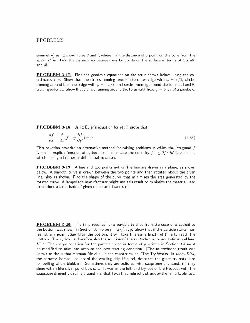
PROBLEM 3-19: A line and two points not on the line are drawn in a plane, as shownbelow. A smooth curve is drawn between the two points and then rotated about the givenline, also as shown. Find the shape of the curve that minimizes the area generated by therotated curve. A lampshade manufacturer might use this result to minimize the material usedto produce a lampshade of given upper and lower radii.

PROBLEM 3-20: The time required for a particle to slide from the cusp of a cycloid tothe bottom was shown in Section 3.4 to be t = π

√a/2g. Show that if the particle starts from

rest at any point other than the bottom, it will take this same length of time to reach thebottom. The cycloid is therefore also the solution of the tautochrone, or equal-time problem.Hint: The energy equation for the particle speed in terms of y written in Section 3.4 mustbe modified to take into account the new starting condition. [The tautochrone result wasknown to the author Herman Melville. In the chapter called “The Try-Works” in Moby-Dick,the narrator Ishmael, on board the whaling ship Pequod, describes the great try-pots usedfor boiling whale blubber: “Sometimes they are polished with soapstone and sand, till theyshine within like silver punchbowls. ... It was in the lefthand try-pot of the Pequod, with thesoapstone diligently circling around me, that I was first indirectly struck by the remarkable fact,

CHAPTER 3

that in geometry all bodies gliding along the cycloid, my soapstone for example, will descendfrom any point in precisely the same time.”]

PROBLEM 3-21: Derive Snell’s law from Fermat’s Principle.

PROBLEM 3-22: A lifeguard stands on the beach a distance l1 from the shoreline. Aswimmer calls for help, a distance l2 directly out from the shoreline and a lateral distance hfrom the lifeguard. If the lifeguard can run twice as fast as she can swim, at what angle θshould she run relative to the shoreline in order to reach the swimmer as soon as possible?

PROBLEM 3-23: Assume Earth’s atmosphere is essentially flat, with index of refractionn = 1 at the top and n = n(y) below, with y measured from the top, and the positive ydirection downward. Suppose also that n2(y) = 1 + αy, where α is a constant. Find thelight-ray trajectory x(y) in this case.

PROBLEM 3-24: Suppose the Earth’s atmosphere is as described in the preceding problem,except that n2(y) = 1 +αy+ βy2, where α and β are constants. Find the light-ray trajectoryx(y) in this case.

PROBLEM 3-25: Consider Earth’s atmosphere to be spherically symmetric above thesurface, with index of refraction n = n(r), where r is measured from the center of the Earth.Using polar coordinates r, θ to describe the trajectory of a light ray entering the atmospherefrom high altitudes, (a) find a first-order differential equation in the variables r and θ thatgoverns the ray trajectory; (b) show that n(r)r sinϕ = constant along the ray, where ϕ is theangle between the ray and a radial line extending outward from the center of the Earth. Thisis the analog of the equation n(y) sin θ = constant for a flat atmosphere.

PROBLEM 3-26: Using the result found in part (b) of the preceding problem, and sup-posing that n2(r) = 1 + α/r2 (where α is a constant), find the light-ray trajectory r(θ).

PROBLEM 3-27: According to Einstein’s general theory of relativity, light rays are deflectedas they pass by a massive object like the Sun. The trajectory of a ray influenced by a central,spherically symmetric object of mass M lies in a plane with coordinates r and θ (so-calledSchwarzschild coordinates); the trajectory must be a solution of the differential equation

d2u

dθ2+ u =

3GM

c2u2 (3.89)

where u = 1/r, G is Newtons gravitational constant, and c is the constant speed of light. (a)The right-hand side of this equation is ordinarily small. In fact, the ratio of the right-handside to the second term on the left is 3GM/rc2. Find the numerical value of this ratio atthe surface of the Sun. The Sun’s mass is 2.0 × 1030 kg and its radius is 7 × 105 km. (b)If the right-hand side of the equation is neglected, show that the trajectory is a straight line.(c) The effects of the term on the right-hand side have been observed. It is known that lightbends slightly as it passes by the Sun and that the observed deflection agrees with the valuecalculated from the equation. Near a black hole, which may have a mass comparable to that

PROBLEMS

of the Sun but a much smaller radius, the right-hand side becomes very important, and therecan be large deflections. In fact, show that there is a single radius at which the trajectoryof light is a circle orbiting the black hole, and find the radius r of this circle. (d) Supposewe wish to make a spherical piece of glass with a varying index of refraction n(r), such thattrajectories of light rays within it will be exactly the same as the trajectories of light around ablack hole. Find the index n(r) required to do this.

PROBLEM 3-28: A clock is thrown straight upward on an airless planet with uniformgravity g, and it falls back to the surface at a time tf after it was thrown, according to clocksat rest on the ground. (a) Using the clock’s motion as derived in Section 3.7, how much moretime than tf will have elapsed according to this moving clock, in terms of g, tf , and c, thespeed of light? (b) Now suppose that instead of the freely-falling motion used in part (a),the moving clock has constant speed v0 straight up for time tf/2 according to ground clocks,and then moves straight down again at the same constant speed v0 for another time intervaltf/2, according to ground clocks. How much more time than tf will have elapsed accordingto this moving clock, in terms of v0, g, c, and tf? (c) Now find the value of v0, keeping g andtf fixed, which maximizes the final reading of the moving clock described in part (b). Thenevaluate the final reading of this moving clock in terms of g, tf , and c, and show that it isless than the final reading of the freely-falling clock described in part (a). (This is a particularillustration of the fact that the path which maximizes the proper time is that of a freely-fallingclock, i.e., , a clock that moves according to Newton’s laws. The reader could choose somealternative motion for a clock, and show again that as long as it returns to the beginning pointat tf according to ground clocks, its time will be less than that of the freely-falling clock ofpart (a).)

PROBLEM 3-29: (a) An automobile driver, stopped at an intersection, ties a helium-filledballoon on a string attached to the floor of her car, so the balloon floats up. When the lightturns green she accelerates the car forward. Relative to the car, does the balloon move forward,backward, or remain vertically above the place it is tied? (b) A rectangular fish tank is halffilled with water. One end of a rubber band is attached to the bottom of the tank, and theother end is attached to a cork that floats on the water’s surface, as shown in the diagram.Now the tank is pushed to the right, giving it a constant rightward acceleration. Eventually,the water surface, cork, and rubber band settle into a new equilibrium configuration. Sketchthis new configuration.

PROBLEM 3-30: A skyscraper elevator comes equipped with two weighing scales: Thefirst is a typical bathroom scale containing springs that compress when someone stands on it,

CHAPTER 3

and the second is the type often used in doctor’s offices, where weights are adjusted to balancethat of the patient. (a) A rider enters the elevator at the ground floor and stands on the firstscale; it reads 150 lbs. Use the principle of equivalence to answer the following questions. (i)As the elevator accelerates upward, will the scale read less than, more than, or equal to 150lbs? (ii) When the elevator reaches its maximum speed and continues rising at this speed, willthe scale read less than, more than, or equal to 150 lbs? (iii) And as the elevator comes torest at the top floor, what will it read? (b) The rider repeats the experiment, standing thistime on the second scale. What will it read during each portion of the trip?

PROBLEM 3-31: A laser is aimed horizontally near Earth’s surface, a distance y0 abovethe ground; a pulse of light is then emitted. (a) How far will the pulse fall by the time it hastravelled a distance L? (b) What is the value of L if the pulse falls by 0.1 nm, roughly thediameter of a hydrogen atom?

PROBLEM 3-32: (a) Show that the pressure difference between two points in an incom-pressible liquid of density ρ in static equilibrium is ∆P = ρgs, where s is the vertical separationbetween the two points and g is the local gravitational field. (b) The liquid is caused to flowthrough a horizontal pipe of varying cross-sectional area, so that its velocity depends uponposition. In a particular section of pipe of length s, the pipe is narrowing, so that the fluid’sacceleration has the constant value a. Find the pressure difference ∆P between one end of thesection and the other, in terms of ρ and the change in the velocity squared (v2) between thetwo ends of the section. Is the pressure larger or smaller at the narrower end of the section?(The result is an example of the Bernoulli effect).

PROBLEMS

Pierre de Fermat (1601 - 1665)

Documents

Transcript of Pierre de Fermat (1601 - 1665)