
Pierre Auger Observatory: Fluorescence Detector Event...
216
UNIVERSITA’ DEGLI STUDI DI CATANIA FACOLTA’ DI SCIENZE MATEMATICHE, FISICHE E NATURALI DOTTORATO DI RICERCA IN FISICA - XVIII CICLO Domenico D’Urso Pierre Auger Observatory: Fluorescence Detector Event Reconstruction and Data Analysis Tutor: Prof. A. Insolia Tutor: Dott. F. Guarino Coordinatore: Prof. F. Riggi Tesi per il conseguimento del titolo
Transcript of Pierre Auger Observatory: Fluorescence Detector Event...
UNIVERSITA’ DEGLI STUDI DI CATANIA
FACOLTA’ DI SCIENZE MATEMATICHE, FISICHE E NATURALIDOTTORATO DI RICERCA IN FISICA - XVIII CICLO
Domenico D’Urso
Pierre Auger Observatory:Fluorescence DetectorEvent Reconstruction
and Data Analysis
Tutor: Prof. A. Insolia
Tutor: Dott. F. Guarino
Coordinatore: Prof. F. Riggi
Tesi per il conseguimento del titolo
Per correr miglior acque alza le vele
omai la navicella del mio ingegno,
che lascia dietro a se mar sı crudele;
e cantero di quel secondo regno
dove l’umano spirito si purga
e di salire al ciel diventa degno.
Dante Alighieri, Divina Commedia: Purgatorio,
Canto I vv. 1-6.

Acknowledgements
I would like to acknowledge the inestimable help I received in writing
this thesis from my friends of the Naples Auger group. They helped
me in many different ways.
My thanks go out to my supervisor Prof. A. Insolia and to his patience
during these three years.
Especially, I would like to thank Laura for the peaceful background
she gave me in the most endless days.
I would like also to thank all my friends, which never have made me
fill alone.
Finally, I would like to thank my family that have always loved me
with all my caprices, defects and faults.
Contents
Introduction v
1 UltraHigh Energy Cosmic Rays 1
1.1 A few historical notes . . . . . . . . . . . . . . . . . . . . . . . . . 1
1.2 The Physics of UHECR . . . . . . . . . . . . . . . . . . . . . . . 3
1.2.1 Cosmic Ray Spectrum . . . . . . . . . . . . . . . . . . . . 4
1.2.2 Cosmic Ray Mass Composition . . . . . . . . . . . . . . . 8
1.2.3 The GZK Limit . . . . . . . . . . . . . . . . . . . . . . . 9
1.3 Possible Sources of UHECR . . . . . . . . . . . . . . . . . . . . . 14
1.3.1 Acceleration and Propagation of cosmic rays . . . . . . . . 18
1.3.1.1 Bottom-up acceleration mechanisms . . . . . . . 18
1.3.1.2 Direct Acceleration Mechanisms . . . . . . . . . . 18
1.3.1.3 The Fermi mechanism . . . . . . . . . . . . . . . 19
1.3.1.4 Top-down acceleration mechanisms . . . . . . . . 23
1.3.1.5 Cosmic ray Propagation . . . . . . . . . . . . . . 23
1.4 Experimental Outlook: Extensive Air Showers . . . . . . . . . . . 25
1.4.1 Shower Development . . . . . . . . . . . . . . . . . . . . . 25
1.4.1.1 The Electromagnetic Component . . . . . . . . . 30
1.4.1.2 The Muon Component . . . . . . . . . . . . . . . 34
1.4.1.3 The Hadron Component . . . . . . . . . . . . . . 35
1.4.2 The Longitudinal Development . . . . . . . . . . . . . . . 37
1.4.3 The Lateral Extension . . . . . . . . . . . . . . . . . . . . 39
1.4.4 Time Structure . . . . . . . . . . . . . . . . . . . . . . . . 42
1.4.5 Fluctuations in Shower Development . . . . . . . . . . . . 44
1.4.6 The Fluorescence Light . . . . . . . . . . . . . . . . . . . . 45
i
CONTENTS
1.4.6.1 Cerenkov, Rayleigh and Mie Contaminations . . 49
1.4.7 UHECR Detection . . . . . . . . . . . . . . . . . . . . . . 53
1.4.7.1 Indirect Techniques . . . . . . . . . . . . . . . . . 54
1.4.8 Fingerprints of primary species in EAS . . . . . . . . . . . 56
1.4.8.1 Muon Component . . . . . . . . . . . . . . . . . 56
1.4.8.2 Elongation Rate . . . . . . . . . . . . . . . . . . 57
1.4.8.3 Temporal Distribution Of Shower Particles . . . . 58
1.4.8.4 Lateral Distribution . . . . . . . . . . . . . . . . 58
2 The Pierre Auger Observatory 59
2.1 Introduction . . . . . . . . . . . . . . . . . . . . . . . . . . . . . . 59
2.2 The Hybrid Detector . . . . . . . . . . . . . . . . . . . . . . . . . 60
2.3 The Southern Observatory . . . . . . . . . . . . . . . . . . . . . . 63
2.4 The Surface Array . . . . . . . . . . . . . . . . . . . . . . . . . . 65
2.4.1 SD Calibration . . . . . . . . . . . . . . . . . . . . . . . . 66
2.5 The Fluorescence Detector . . . . . . . . . . . . . . . . . . . . . . 67
2.5.1 FD Detector Calibration . . . . . . . . . . . . . . . . . . . 74
2.5.1.1 Absolute Calibration . . . . . . . . . . . . . . . . 75
2.5.1.2 Relative Calibration . . . . . . . . . . . . . . . . 77
2.6 Atmospheric Monitoring . . . . . . . . . . . . . . . . . . . . . . . 80
3 Event Reconstruction with Pierre Auger Data 84
3.1 Introduction . . . . . . . . . . . . . . . . . . . . . . . . . . . . . . 84
3.2 FD Data Acquisition Strategy . . . . . . . . . . . . . . . . . . . . 86
3.2.1 First Level Trigger . . . . . . . . . . . . . . . . . . . . . . 86
3.2.2 Second Level Trigger . . . . . . . . . . . . . . . . . . . . . 87
3.2.3 Third Level Trigger . . . . . . . . . . . . . . . . . . . . . . 87
3.2.4 The T3 trigger . . . . . . . . . . . . . . . . . . . . . . . . 88
3.3 SD Trigger and Data Selection . . . . . . . . . . . . . . . . . . . . 89
3.3.1 Tank Level Triggers . . . . . . . . . . . . . . . . . . . . . . 90
3.3.2 Event Selection Triggers . . . . . . . . . . . . . . . . . . . 91
3.3.3 T5 quality Trigger . . . . . . . . . . . . . . . . . . . . . . 91
3.4 Hybrid Trigger . . . . . . . . . . . . . . . . . . . . . . . . . . . . 93
3.5 SD Event Reconstruction . . . . . . . . . . . . . . . . . . . . . . . 94
ii
CONTENTS
3.5.1 SD Geometry Reconstruction . . . . . . . . . . . . . . . . 94
3.5.2 SD Energy Estimation . . . . . . . . . . . . . . . . . . . . 96
3.6 FD Event Reconstruction . . . . . . . . . . . . . . . . . . . . . . 97
3.6.1 Geometrical Reconstruction . . . . . . . . . . . . . . . . . 98
3.6.1.1 Shower Detector Plane Reconstruction . . . . . . 99
3.6.1.2 Shower Axis Reconstruction . . . . . . . . . . . . 100
3.6.2 Longitudinal Profile Reconstruction . . . . . . . . . . . . . 104
3.6.2.1 Energy Estimation . . . . . . . . . . . . . . . . . 106
3.6.3 Systematic Uncertainties . . . . . . . . . . . . . . . . . . . 107
3.7 The Offline Software Framework of the Pierre Auger Observatory 108
4 Application of Gnomonic Projection to the SDP reconstruction
for FD events 111
4.1 Introduction . . . . . . . . . . . . . . . . . . . . . . . . . . . . . . 111
4.2 Reconstruction strategy . . . . . . . . . . . . . . . . . . . . . . . 112
4.2.1 Pixel Selection . . . . . . . . . . . . . . . . . . . . . . . . 113
4.2.2 Definition of coordinates . . . . . . . . . . . . . . . . . . . 114
4.2.3 Gnomonic Projection approach to SDP reconstruction . . 115
4.3 Performances of the method . . . . . . . . . . . . . . . . . . . . . 118
4.3.1 Resolution on SDP reconstruction . . . . . . . . . . . . . 119
4.4 Effect of improved SDP resolution on shower reconstruction . . . 124
4.5 A first look at CORSIKA showers . . . . . . . . . . . . . . . . . . 125
5 FD reconstruction accuracy studies by means of CLF laser shots131
5.1 Introduction . . . . . . . . . . . . . . . . . . . . . . . . . . . . . . 131
5.2 Analysis Strategy . . . . . . . . . . . . . . . . . . . . . . . . . . . 132
5.3 Angular Resolution . . . . . . . . . . . . . . . . . . . . . . . . . . 134
5.4 Core Determination . . . . . . . . . . . . . . . . . . . . . . . . . . 138
5.5 Telescope Alignment . . . . . . . . . . . . . . . . . . . . . . . . . 141
5.5.1 Alignment Technique . . . . . . . . . . . . . . . . . . . . . 142
5.5.1.1 CLF Laser Shots Sample Selection . . . . . . . . 143
5.5.1.2 Sheaf Center Determination . . . . . . . . . . . . 143
5.5.2 Alignment Tests . . . . . . . . . . . . . . . . . . . . . . . . 147
iii
CONTENTS
6 Analysis of FD Data 153
6.1 Introduction . . . . . . . . . . . . . . . . . . . . . . . . . . . . . . 153
6.2 Reconstruction Accuracy and
Definition Of Analysis Cuts . . . . . . . . . . . . . . . . . . . . . 154
6.2.1 The Simulated Data Sample . . . . . . . . . . . . . . . . . 154
6.2.2 Definition of Analysis Cuts . . . . . . . . . . . . . . . . . . 155
6.2.2.1 Shower Detector Plane . . . . . . . . . . . . . . . 157
6.2.2.2 Shower Axis . . . . . . . . . . . . . . . . . . . . . 160
6.2.2.3 Longitudinal Shower Profile . . . . . . . . . . . . 160
6.2.3 Application Of Analysis Cuts To Real Data . . . . . . . . 166
6.2.4 Summary . . . . . . . . . . . . . . . . . . . . . . . . . . . 172
6.3 Reconstruction of Real FD Events . . . . . . . . . . . . . . . . . 172
6.4 Analysis Results . . . . . . . . . . . . . . . . . . . . . . . . . . . . 178
6.4.1 All Particle Spectrum . . . . . . . . . . . . . . . . . . . . . 178
6.4.1.1 Detector Aperture . . . . . . . . . . . . . . . . . 179
6.4.1.2 Live Time Determination . . . . . . . . . . . . . 182
6.4.1.3 Spectrum Evaluation . . . . . . . . . . . . . . . . 182
6.4.2 Elongation Rate . . . . . . . . . . . . . . . . . . . . . . . . 186
6.5 Conclusions . . . . . . . . . . . . . . . . . . . . . . . . . . . . . . 191
Conclusions 192
Bibliography 194
iv
Introduction
The cosmic ray story begins about 1900: 100 years later most of the main issues
are still open questions, as sources, acceleration mechanisms, propagation and
composition, especially for the extremely high energy cosmic rays, around 1020
eV .
The Pierre Auger Observatory is the biggest experiment on cosmic rays even
conceived and it has been designed in order to solve the fascinating cosmic ray
puzzle. The experiment involves several universities and research institutes from
18 countries, a collaboration with more than 300 physicists. The project consists
of a two-sites observatory, one for each terrestrial hemisphere. The Southern
Observatory will be completed st the end of 2006. It is located i the Pampa
Amarilla, in the Mendoza Province, Argentina. The Northen Observatory will
be built in Colorado. Each site will instrument a 3000 km2 area with an array
of particle detectors, water Cerenkov detectors, overlooked by a group of fluo-
rescence telescopes, disposed at the edges of the area, within 4 buildings, called
eye. Both detection techniques have been well established, separately, by prior
experiments. The combined use of these two techniques can allow: to achieve an
unprecedented reconstruction accuracy, to perform cosmic ray energy measure-
ments almost model independent; to study systematic effects inherent to either
methods alone; to measure a wide set of shower parameters in order to identify
cosmic ray mass composition.
In this thesis, I will discuss original contributions to fluorescence detector
event reconstruction and analysis: new algorithm implmentation for geometrical
reconstruction of fluorescence events; reconstruction accuracy studies; telescope
misalignment measurement; determination of detector reconstruction efficiency
v
and live time; first estimation of all particle data spectrum and elongation rate
with fluorescence data.
The first chapter is an introduction to main aspects of ultra high energy cosmic
ray physics. It describes extended air shower development and the production of
fluorescence light in the case of shower with energy above 1017 eV .
In the second chapter, main characteristics of Pierre Auger Observatory are
presented: the Fluorescence detector, the Surface detector and briefly the atmo-
spheric monitoring.
The event trigger and reconstruction strategy are described in chapter 3.
There is a description of all level trigger used in the Fluorescence and Surface de-
tector data acquisition and of the hybrid trigger strategy, which allows to combine
the use of the two different techniques. Event reconstruction are presented step
by step in the case of pure Surface array events, of pure Fluorescence detector
events and of hybrid events.
Chapter 4 is completely devoted to the discussion of the use of gnomonic pro-
jections in the Fluorescence detector event reconstruction. Gnomonic projections
allow to reduce the usual procedure (derived from Fly’s Eye experiment, first to
use the fluorescence technique to study cosmic ray showers) of computing the
shower detector plane - namely the plane containing the shower trajectory and
the observation point - to a linear fit, once the spherical surface of telescope ac-
tive camera, made by 440 photomultiplier, is projected into a gnomonic plane.
In the same chapter, a few tools, developed to perform the rejection noise photo-
multiplier, are also described. Finally the comparison of this technique and the
standard Fly’s Eye method, over a large set of simulated showers, at different
energies and geometrical configurations, and its effects on the reconstruction of
shower energy and the depth of shower maximum is discussed.
In chapter 5, the improved event reconstruction is tested by means of laser
shots of known geometry produced by a Laser Facility located in the middle
of the ground array, which is able to send a fraction of laser light to a nearby
water detector and to produce an hybrid detection of laser shots. Geometrical
reconstruction accuracy are derived for mono (events recorded only by one eye
of the Fluorescence detector), hybrid (events recorded by both detector) and
stereo (events recorded by at least two eyes). In the second part of chapter 5,
vi
laser shots and gnomonic projections are used to develop a new technique to
measure telescope misalignments observed in the reconstruction accuracy study.
Corrections to telescope pointing directions are then applied to laser shot stereo
reconstruction.
Chapter 6 is dedicated to extract first physical informations from Auger Flu-
orescence data: cosmic ray energy spectrum and elongation rate. The simulated
data sample used to estimate Fluorescence detector aperture have been used to
define useful criteria required to acquire an accurate shower reconstruction and
calculate reconstruction efficiency at different energies. Defined cuts are applied
in the analysis of Fluorescence detector data from january 2004 to november 2005.
The use of the Fluorescence detector apertures available within the Auger Col-
laboration is described. The Fluorescence detector live time has been computed
monitoring detectot evolution and operation in time. Finally, the first estimate
of the all particle spectrum produced with Fluorescence detector data only is
given. The data set used to produce the energy spectrum is also employed to
give a preliminary elongation rate, comparing obtained data with those coming
from simulation of different primary species.
vii
Chapter 1
UltraHigh Energy Cosmic Rays
1.1 A few historical notes
The Earth’s atmosphere is continuosly bombarded by extraterrestrial particles,
the so called Cosmic Rays (CR), which consist of ionized nuclei, mainly protons,
alpha particles and heavier nuclei. Most of them are relativistic and a few par-
ticles have an ultrarelativistic kinetic energy, extending up to 1020 eV . This is a
macroscopic energy, equivalent to that one of a tennis ball moving at 100 km/h.
CR story starts at the beginning of the 20th century when it was found that
electroscopes discharged even in the dark, well away from sources of natural
radioactivity. To solve the puzzle, in 1912 Hess [1] and successively Kolhorster [2]
made a series of manned balloon flights, in which they measured the ionization of
the atmosphere with increasing altitude. What they found out was the startling
result that the average ionization increases with respect to its value at the sea-level
(at 5000 m the difference between observed ionization and that at sea-level was of
∼ 17 × 108 ions m−3) as if a radiation with high penetrating power would arrive
from outside the Earth. Eventually the term Cosmic Rays was used by Millikan
in a seminar at the Leeds University (UK) and, since then, used throughout.
At the beginning, the community believed that CR were “high” energy pho-
tons (at that time the most penetrating radiation known was γ rays). Just in
1929, using a “new” detector able to detect individual cosmic rays, the Geiger-
Muller counter, Bothe and Kolhorster showed that CR were mainly composed by
charged particles and, because of their long range in the matter, these particles
1
1.1 A few historical notes
would have to be very energetic (∼ 109 eV ). From this hypothesis, Bruno Rossi
started to study secondary particle production through interaction of CR with
matter, so called “showers”.
In 1934, on the basis of his observations in Eritrea, Rossi [3] reported of strange
coincidences between different detectors as if very extensive groups of particles
arrived all at once upon the detector. With the use of the first coincidence
circuit at ∼ 5 × 10⁻⁶ s, Pierre Auger and his group [4] discovered that some
cascades were initiated by CR, interacting with the atmosphere. Auger called
these cascades Extensive Air Showers (EAS). At that time the primary cosmic
rays were thought to contain a large amount of electrons and a new theory,
developed by Bethe and Heitler [5], was used to infer the primary energy. EAS
studies continued using larger arrays of Geiger-Muller counters, and events with
an energy larger than 1017 eV were detected.
From CR studies the elementary particle physics was born. Indeed, from
cosmic radiation track studies with cloud chamber, Blackett and Occhialini [6]
in 1933 discovered the positron and in 1936 Anderson and Neddermeyer [7] an-
nounced the observation of particles with mass intermediate between that one of
the electron and the proton, the muon. With a new kind of instrument, nuclear
emulsion, in 1947 there was the observation of the pion by Rochester and Butler
[8] and so on till the Σ particle discovery in 1953 [9]. Since then elementary
particle physics was able to use a new kind of “high” energy particle source, ac-
celerators, its future laid in accelerator laboratory rather than in the cosmic ray
observations. The interest in CR shifted to the problems of their origin and their
propagation through the space, from their sources to the Earth.
Although a century of adventurous researches and detailed studies is passed,
cosmic ray radiation still shows unanswered questions. In the last forty years,
many hundreds peculiar events were recorded, in which Extensive Air Showers
were generated by a primary particle whose energy was estimated to exceed 1018
eV (Ultra High Energy Cosmic Rays, UHECR), by different cosmic ray experi-
ments, such as AGASA [10; 11; 12], Fly’s Eye [13] and the High Resolution Fly’s
Eye [14], Haverah Park [15], Yakutsk [16], and more recently the Pierre Auger
experiment [27]. Usually, the most energetic component of UHECR, primary
particles with energy above 5 × 10¹⁹ eV is indicated as Extremely High Energy
2
1.2 The Physics of UHECR
Cosmic Rays (EHECR) and its existence opened issues that constitute a puz-
zle still today, whose solution involves astronomy and cosmology, nuclear physics
and elementary particle physics: origin, acceleration mechanisms, propagation,
high energy interaction in the EAS above the highest feasible energy with accel-
erators (LHC experiment will work up to 1012 eV in the center-of-masse frame,
equivalent to ∼ 1017 eV in the laboratory frame).
1.2 The Physics of UHECR
There is a continuing fascination with the studies of Ultra High-Energy Cosmic
Rays, mostly from several contradictions connected to their obseration.
One of the reason of interest concerns their origin: the places where they
are produced are probably astrophysical sites containing unusual large energies
in their magnetic field structures (see Greisen [17]). Such sources are relatively
rare and mostly far from the Earth. Particles travelling from these sources to
us should interact with Cosmic Background Radiation, deeply modifying the ob-
served energy spectrum, causing the expected Greisen-Zatsepin-Kuzmin (GZK)
cutoff (Greisen [18], Zatsepin and Kuzmin [19]). So the observation of a particle
with energy > 1020 eV would imply that its source lays within ∼ 100 Mpc from
the Earth. At this energy, estimated galactic and extra-galactic fields are such
that they should modify negligibly particle trajectories. Therefore, primary ar-
rival directions should point back directly at sources. But in high energy events
observed till now, there is no clear anisotropy. Even a more important is the
understanding of the mechanism responsible for production and acceleration able
to bring primary particles at this very high energy.
In this energy range, due to the very low flux1 experimental statistics is very
poor. Due to this luck of statistics and experimental uncertainties2, it is not yet
established if the GZK cut-off is actually visible in the data or not.
1The measured CR flux above 1020 eV is of one particle for kilometer square for century.2Most of cosmic ray studies depend on phenomenological models. They are based on Stan-
dard Model physics extrapolated to energies of several order higher than those achievable incurrent and future collider experiments. Furtheremore, processes involved are in kinematicregions unexplored in the study of fundamental interactions.
3
1.2 The Physics of UHECR
1.2.1 Cosmic Ray Spectrum
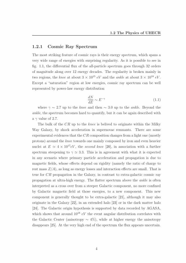
The most striking feature of cosmic rays is their energy spectrum, which spans a
very wide range of energies with surprising regularity. As it is possible to see in
fig. 1.1, the differential flux of the all-particle spectrum goes through 32 orders
of magnitude along over 12 energy decades. The regularity is broken mainly in
two regions, the knee at about 3 × 10¹⁵ eV and the ankle at about 3 × 10¹⁸ eV .
Except a “saturation” region at low energies, cosmic ray spectrum can be well
represented by power-law energy distribution
dN
dE∼ E−γ (1.1)
where γ ∼ 2.7 up to the knee and then ∼ 3.0 up to the ankle. Beyond the
ankle, the spectrum becomes hard to quantify, but it can be again described with
a γ value of 2.7.
The bulk of the CR up to the knee is belived to originate within the Milky
Way Galaxy, by shock acceleration in supernovae remnants. There are some
experimental evidences that the CR composition changes from a light one (mostly
protons) around the knee towards one mainly composed by iron and even heavier
nuclei at E 4 × 10¹⁷eV , the second knee [20], in association with a further
spectrum steepening to γ 3.3. This is in agreement with what it is expected
in any scenario where primary particle acceleration and propagation is due to
magnetic fields, whose effects depend on rigidity (namely the ratio of charge to
rest mass Z/A), as long as energy losses and interaction effects are small. That is
true for CR propagation in the Galaxy, in contrast to extra-galactic cosmic ray
propagation at ultra-high energy. The flatter spectrum above the ankle is often
interpreted as a cross over from a steeper Galactic component, no more confined
by Galactic magnetic field at those energies, to a new component. This new
component is generally thought to be extra-galactic [21], although it may also
originate in the Galaxy [22], in an extended halo [23] or in the dark matter halo
[24]. The Galactic origin hypothesis is supported by data recorded by AGASA,
which shows that around 1018 eV the event angular distribution correlates with
the Galactic Center (anisotropy ∼ 4%), while at higher energy the anisotropy
disappears [25]. At the very high end of the spectrum the flux appears uncertain.
4
1.2 The Physics of UHECR
Figure 1.1: All-particle energy spectrum from a compilation of measurements of
the differential energy spectrum of CR. The dotted line shows an E−3 power-law
distribution for comparison. Approximate integral fluxes are also shown.
5
1.2 The Physics of UHECR
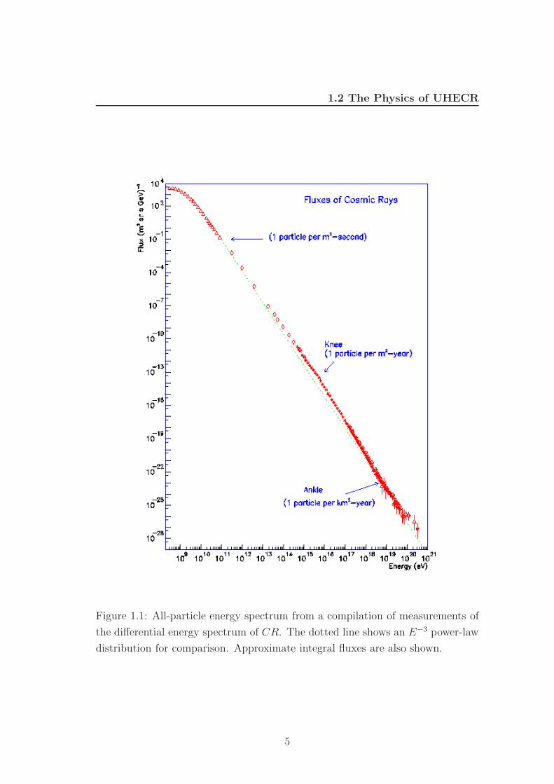
Indeed, the most recent experiments, AGASA and HiRes, reported a number of
events above 1020 eV completely in disagreement: HiRes collected only 2 events
instead of about 20 expected for a spectrum similar to that reported by AGASA
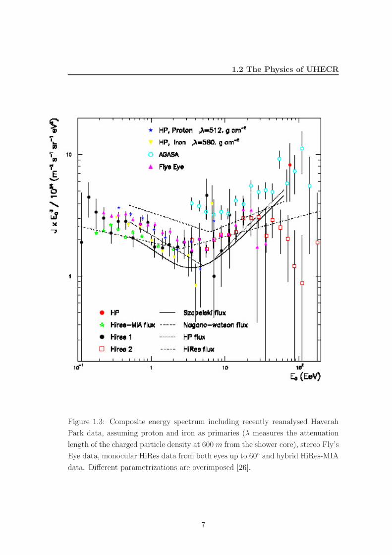
[26] (17 events above 1020 eV ) (see fig. 1.2). Figure 1.3 shows the comparison
among Fly’s Eye, HiRes, AGASA and Haverah Park data.
Figure 1.2: High energy cosmic ray spectrum multiplied by E3 to evidence its
features, as seen by AGASA (blue ), by HiRes-II (black ) and HiRes-I (red
). The continuous line is the predicted flux coming out from an isotropic source
model.
This question will be addressed and probably solved by the Auger Observatory
data [27], which combine the two complementary detection techniques adopted
by the aforementioned experiments.
6
1.2 The Physics of UHECR
Figure 1.3: Composite energy spectrum including recently reanalysed Haverah
Park data, assuming proton and iron as primaries (λ measures the attenuation
length of the charged particle density at 600 m from the shower core), stereo Fly’s
Eye data, monocular HiRes data from both eyes up to 60 and hybrid HiRes-MIA
data. Different parametrizations are overimposed [26].
7
1.2 The Physics of UHECR
1.2.2 Cosmic Ray Mass Composition
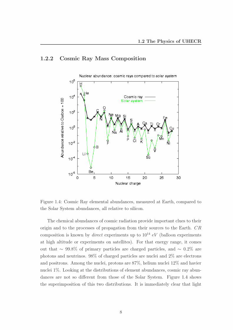
Figure 1.4: Cosmic Ray elemental abundances, measured at Earth, compared to
the Solar System abundances, all relative to silicon.
The chemical abundances of cosmic radiation provide important clues to their
origin and to the processes of propagation from their sources to the Earth. CR
composition is known by direct experiments up to 1014 eV (balloon experiments
at high altitude or experiments on satellites). For that energy range, it comes
out that ∼ 99.8% of primary particles are charged particles, and ∼ 0.2% are
photons and neutrinos. 98% of charged particles are nuclei and 2% are electrons
and positrons. Among the nuclei, protons are 87%, helium nuclei 12% and havier
nuclei 1%. Looking at the distributions of element abundances, cosmic ray abun-
dances are not so different from those of the Solar System. Figure 1.4 shows
the superimposition of this two distributions. It is immediately clear that light
8
1.2 The Physics of UHECR
elements, as lithium, beryllium and boron are grossly overabundant in the cosmic
radiation. There is also an excess of elements just less heavy then those of the iron
group. And finally there is a lack of hydrogen and helium in the cosmic rays with
respect to heavy elements. Some differences can be due to spallation processes:
primary cosmic rays, propagating through the interstellar medium, suffer spalla-
tion collisions with ambient interstellar gas. The net result is the production of
nuclei with atomic and mass numbers just less than those of the common groups
of elements. The overall impression is that cosmic rays have been accelerated
from material of quite similar chemical composition as in the the Solar System.
When it is not possible to perform direct measurements of primary particles
(typically for Eprimary > 1014 eV ), the radiation composition is inferred from
indirect observation. Then conclusions are strongly dependent on models used
to describe the data. Different methods used for mass measurement usually give
different answers.
1.2.3 The GZK Limit
As it is evident from fig. 1.3, cosmic rays of quite enormous energy have been
detected. The first event was observed by Volcano Ranch experiment [28], with
an estimated energy of 1.3 × 10²⁰ eV . In the last forty years, other experiments
registered high energy cosmic rays, Yakutsk, Fly’s Eye, HiRes, AGASA. In
particular, Fly’s Eye observed the most energetic EAS, 3.2± 0.9)× 1020 eV [29].
These events seem to be in disagreement with the GZK-limit. As already
explained, in this energy range, particles should interact with Cosmic Background
Radiation: the relic photon energy is sufficient to excite baryon resonances thus
draining the proton energy via pion production and producing ultrahigh energy
gamma rays and neutrinos. Naively, the GZK-limit gives the radius of the sphere
within which a source has to lie in order to provide us with proton of 1020 eV .
There are three sources of energy loss of ultrahigh energy protons: adiabatic
fractional energy loss due to the expansion of the Universe, pair production (p +
γ → p + e+ + e−) and photopion production (p + γ → π + N), each successively
dominating as the proton energy increases. The adiabatic fractional energy loss
9
1.2 The Physics of UHECR
at the present cosmological epoch is given by
− 1
E
(dE
dt
)adiabatic
= H0 (1.2)
where H0 ∼ 100 h km s−1 Mpc−1 is the Hubble constant, with h ∼ (0.71 ±0.07)×1.15
0.95 the normalized Hubble expansion rate [30]. The fractional energy loss
due to interaction with the cosmic background radiation at redshift z = 0 is
determined by the integral of the nucleon energy loss per collision multiplied by
the probability per unit time for a nucleon collision in an isotropic gas of photons
[31]. Pair production and photopion production are important for interaction
with the 2.7 K blackbody background radiation. Collisions with optical and
infrared photons give a negligible contribution. For interactions with a blackbody
field of temperature T , the photon density is that of the Plank spectrum [32].
The mean interaction length, xpγ of a proton of energy E is given by
1
xpγ(E)=
1
8βE2
∫ ∞
εmin(E)
n(ε)
ε2
∫ smax(ε,E)
smin
σ(s)(s − m2pc
4)dsdε (1.3)
where n(ε) is the differential number density of photons with energy ε, σ(s)
is the appropriate total cross section for the process in question for a center
momentum (CM) frame energy squared s, given by
s = m2pc
4 + 2εE(1 − β cos θ) (1.4)
with θ the angle between the directions of proton and photon and βc the
proton velocity. Threshold values for processes are smin ≈ 0.882 GeV 2 (E ≈
1018 eV ) for pair production and smin ≈ 1.16 GeV 2 for photopion production,
equivalent to the request of
Ethpγ =
mπ(mp + mπ/2)
ε≈ 6.8 × 10¹⁹
( ε
10−3
)−1
eV (1.5)
in the proton rest frame. The cross section for the latter process strongly increases
at the ∆(1232) resonance, which decays into pion channels π+n and π0p. With
increasing energy, heavier baryon resonances occur and the proton might reappear
only after successive decays of resonances. The mean interaction lenghts, derived
from equation 1.3, are plotted as dashed lines in fig. 1.5. Dividing by mean
10
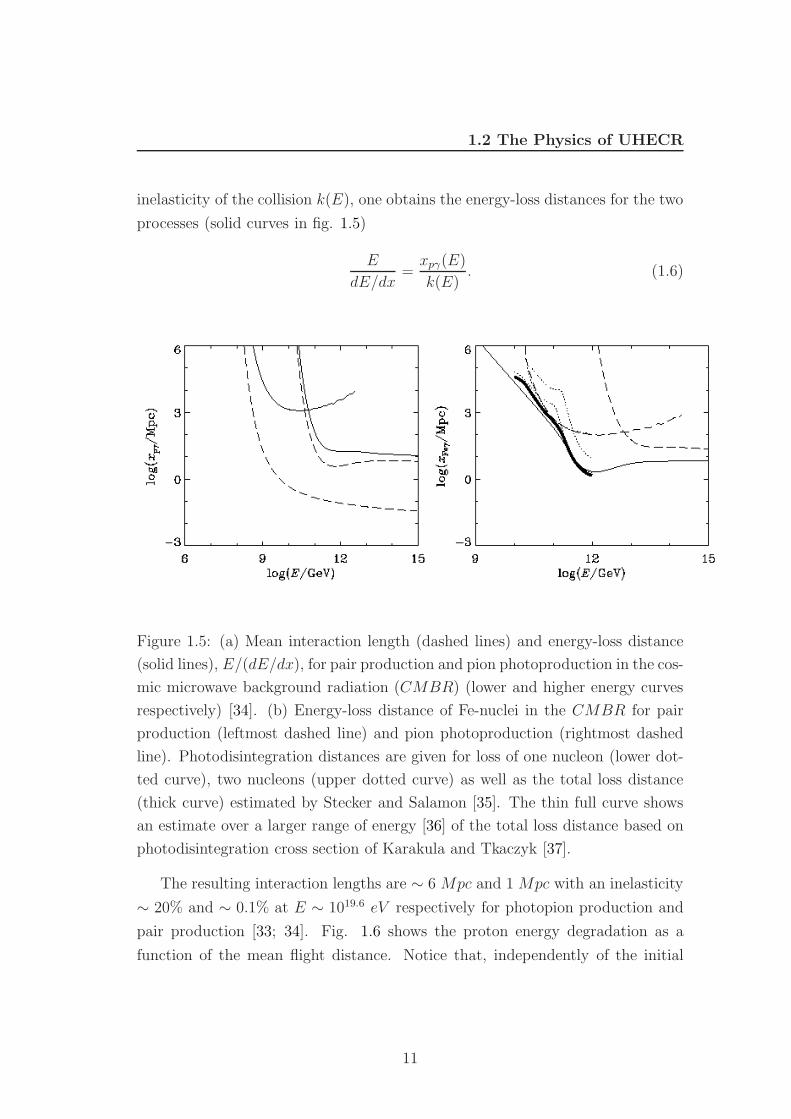
1.2 The Physics of UHECR
inelasticity of the collision k(E), one obtains the energy-loss distances for the two
processes (solid curves in fig. 1.5)
E
dE/dx=
xpγ(E)
k(E). (1.6)
Figure 1.5: (a) Mean interaction length (dashed lines) and energy-loss distance
(solid lines), E/(dE/dx), for pair production and pion photoproduction in the cos-
mic microwave background radiation (CMBR) (lower and higher energy curves
respectively) [34]. (b) Energy-loss distance of Fe-nuclei in the CMBR for pair
production (leftmost dashed line) and pion photoproduction (rightmost dashed
line). Photodisintegration distances are given for loss of one nucleon (lower dot-
ted curve), two nucleons (upper dotted curve) as well as the total loss distance
(thick curve) estimated by Stecker and Salamon [35]. The thin full curve shows
an estimate over a larger range of energy [36] of the total loss distance based on
photodisintegration cross section of Karakula and Tkaczyk [37].
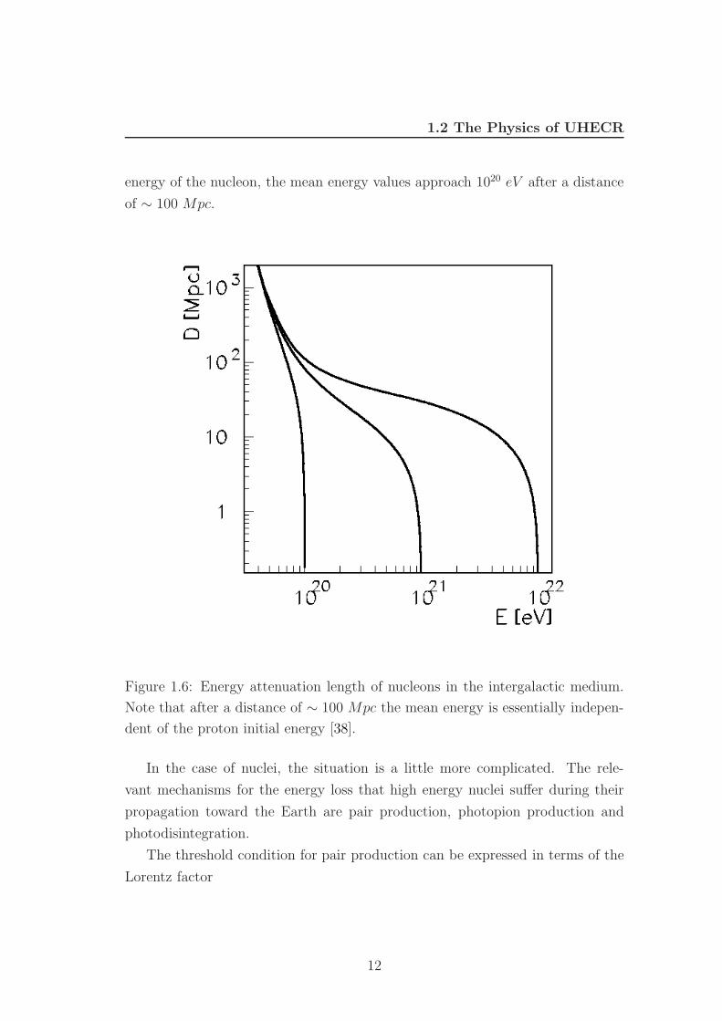
The resulting interaction lengths are ∼ 6 Mpc and 1 Mpc with an inelasticity
∼ 20% and ∼ 0.1% at E ∼ 1019.6 eV respectively for photopion production and
pair production [33; 34]. Fig. 1.6 shows the proton energy degradation as a
function of the mean flight distance. Notice that, independently of the initial
11
1.2 The Physics of UHECR
energy of the nucleon, the mean energy values approach 1020 eV after a distance
of ∼ 100 Mpc.
Figure 1.6: Energy attenuation length of nucleons in the intergalactic medium.
Note that after a distance of ∼ 100 Mpc the mean energy is essentially indepen-
dent of the proton initial energy [38].
In the case of nuclei, the situation is a little more complicated. The rele-
vant mechanisms for the energy loss that high energy nuclei suffer during their
propagation toward the Earth are pair production, photopion production and
photodisintegration.
The threshold condition for pair production can be expressed in terms of the
Lorentz factor
12
1.2 The Physics of UHECR
γ >mec
2
ε
(1 +
me
Amp
)(1.7)
and that one for photopion production as
γ >mπc2
2ε
(1 +
mπ
2Amµ
). (1.8)
Since γ = E/Ampc2, where A is the mass number, both energy-loss distance
curves in fig. 1.5 are shifted by a factor A. For pair production the energy loss
by a nucleus in each collision near the threshold is approximately ∆E ≈ γ2mec2,
hence the inelasticity is ≈ 2me/(Amp), a factor A lower than for protons. On the
other hand, the cross section depends on Z2, so the overall shift is down by Z2/A
(energy loss distance for pair production for iron nuclei is reduced by a factor
≈ 12.1).
For pion production, the energy loss in each collision near the threshold is
∆E ≈ γ2mπc2, so the inelasticity is a factor A lower than for protons. The cross
section increases approximately as A0.9 giving an overall increase in the energy
loss distance of a factor ∼ A0.1 ≈ 1.5 for iron nuclei (see fig. 1.5).
The dominant mechanism of energy loss for nuclei is photodisintegration. The
photodisintegration distance, defined as A/(dA/dx) calculated by Stecker and
Salomon, is shown in fig. 1.5, together with an estimate made over a larger
energy range by Protheroe [36] of the total loss distance based on cross section
of Karakula and Tkaczyk [37].
Neutrons, even at the higher energies, decay into protons after a free fly of
only ∼ 1 Mpc, so they could be ruled out.
In summary, the GZK−cutoff implies that, if the primary ultrahigh energy
cosmic rays are protons, energetic sources should be close to the Earth, within a
distance of the order of 50 − 100 Mpc.
In the case of high energy γ−rays, the dominant absorption process is pair
production through collisions with the radiation fields permeating the Universe.
On the other hand, electrons and positrons could produce new γ−rays via inverse
Compton scattering. The new γ can initiate a fresh cycle of pair production
and inverse Compton scattering interactions, yielding an electromagnetic cascade.
13
1.3 Possible Sources of UHECR
The development of electromagnetic cascades depends sensitively on the strength
of the extragalactic magnetic field B, which is rather uncertain.
The threshold for the pair production process is of the order of m2e/ε, where ε
is the energy of the radiation field involved. Above 1020 eV , the most relevant in-
teractions are those with radio background, which is almost unknown. Therefore,
the GZK radius of the photon strongly depends on the strength of extragalactic
magnetic fields. In principle, distant sources with a redshift z > 0.03 can con-
tribute to the observed cosmic rays above 5×10¹⁹eV if the extragalactic magnetic
field does not exceed 10−12 G [40].
Neutrinos do not suffer any energy degradation during their trip through the
Universe, unless for energies above 1023 eV [42]. As noted by Weiler [43; 44], neu-
trinos can travel over cosmological distances with negligible energy loss and could
produce Z bosons on resonance through annihilation on the relic neutrino back-
ground, within a GZK distance from Earth. In that case, highly boosted decay
products could be observed as super−GZK (above GZK−limit) primaries and
they would point directly back to the source. This model of course requires very
luminous sources of extremely high energy neutrinos through-out the Universe.
1.3 Possible Sources of UHECR
The Main astrophysical question connected to cosmic ray studies is the identifi-
cation of possible UHECR sources and plausible acceleration mechanisms to get
particles above 1020 eV .
The CR energy density measured at the top of the atmosphere is dominated
by low energy component between 1 and 10 GeV . At energies of about 1 GeV
the intensities are correlated with the solar activity. At higher energies (10− 100
GeV ) the flux is anticorrelated with solar activity, indicating an extra-solar origin.
Several arguments involving energetics, composition and secondary γ−ray
production suggest that the bulk of CR (between 1 GeV up to PeV ) is confined
to the galaxy and is probably produced in supernova remnants (SNRs). Between
the knee and the ankle the situation becomes less clear. The ankle is sometimes
interpreted as a cross over from a galactic to an extragalactic component. Fi-
nally, beyond 10 EeV , CR are generally expected to be extragalactic. These
14
1.3 Possible Sources of UHECR
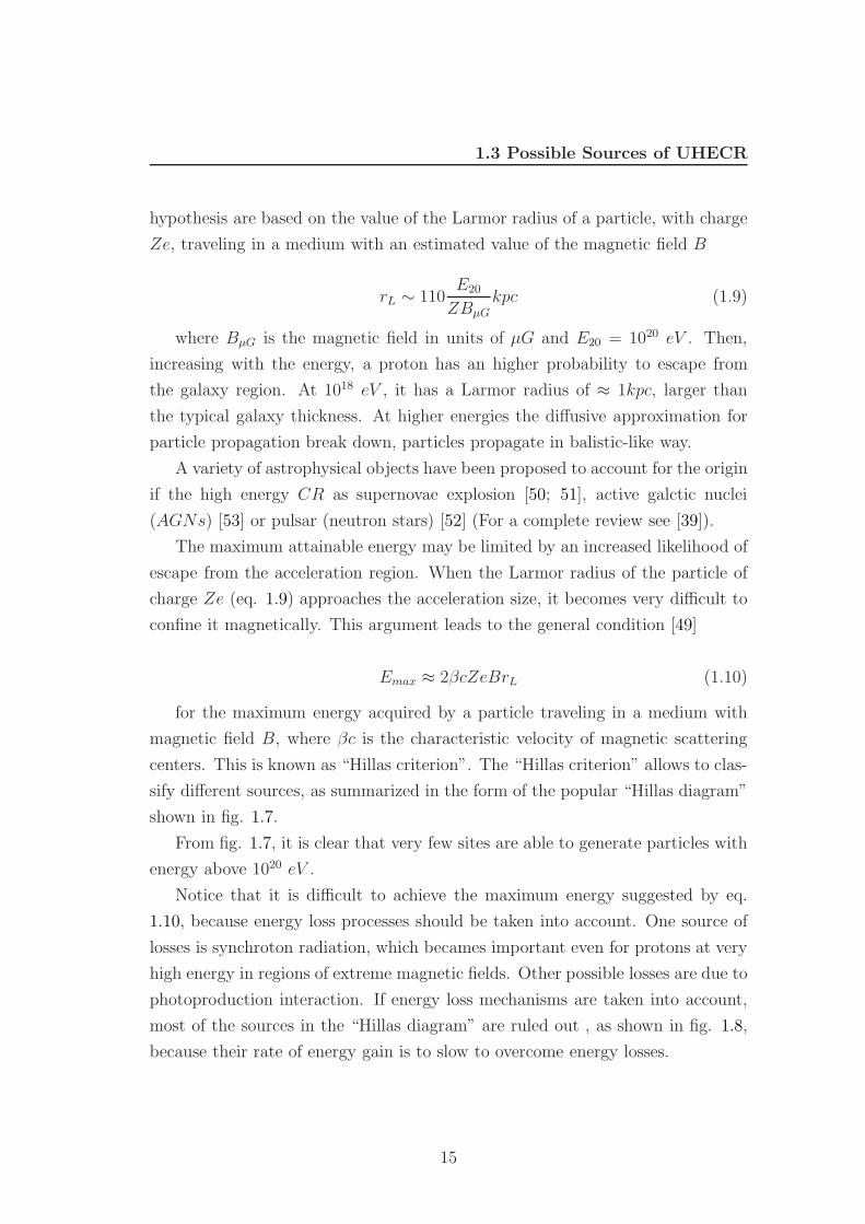
hypothesis are based on the value of the Larmor radius of a particle, with charge
Ze, traveling in a medium with an estimated value of the magnetic field B
rL ∼ 110E20
ZBµG
kpc (1.9)
where BµG is the magnetic field in units of µG and E20 = 1020 eV . Then,
increasing with the energy, a proton has an higher probability to escape from
the galaxy region. At 1018 eV , it has a Larmor radius of ≈ 1kpc, larger than
the typical galaxy thickness. At higher energies the diffusive approximation for
particle propagation break down, particles propagate in balistic-like way.
A variety of astrophysical objects have been proposed to account for the origin
if the high energy CR as supernovae explosion [50; 51], active galctic nuclei
(AGNs) [53] or pulsar (neutron stars) [52] (For a complete review see [39]).
The maximum attainable energy may be limited by an increased likelihood of
escape from the acceleration region. When the Larmor radius of the particle of
charge Ze (eq. 1.9) approaches the acceleration size, it becomes very difficult to
confine it magnetically. This argument leads to the general condition [49]
Emax ≈ 2βcZeBrL (1.10)
for the maximum energy acquired by a particle traveling in a medium with
magnetic field B, where βc is the characteristic velocity of magnetic scattering
centers. This is known as “Hillas criterion”. The “Hillas criterion” allows to clas-
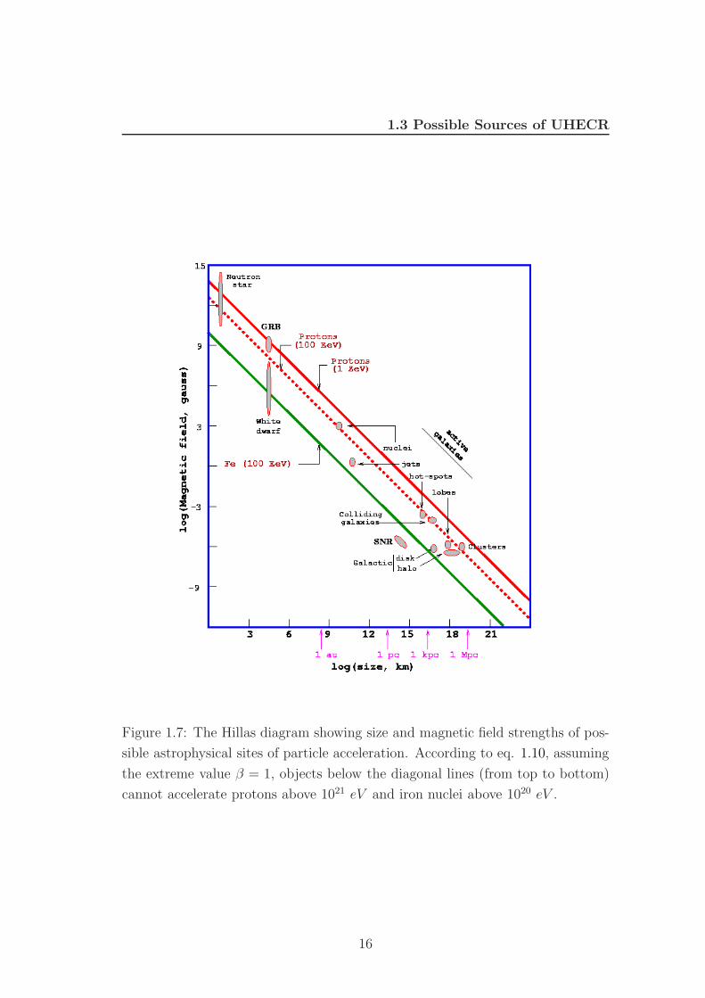
sify different sources, as summarized in the form of the popular “Hillas diagram”
shown in fig. 1.7.
From fig. 1.7, it is clear that very few sites are able to generate particles with
energy above 1020 eV .
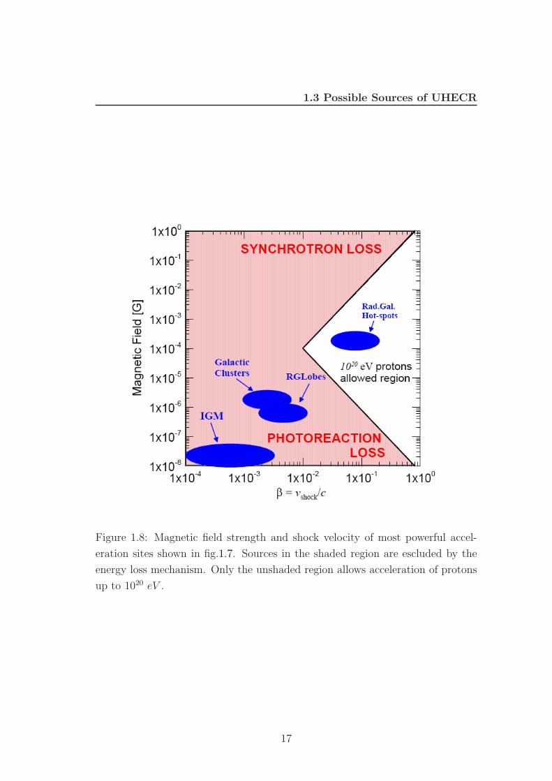
Notice that it is difficult to achieve the maximum energy suggested by eq.
1.10, because energy loss processes should be taken into account. One source of
losses is synchroton radiation, which becames important even for protons at very
high energy in regions of extreme magnetic fields. Other possible losses are due to
photoproduction interaction. If energy loss mechanisms are taken into account,
most of the sources in the “Hillas diagram” are ruled out , as shown in fig. 1.8,
because their rate of energy gain is to slow to overcome energy losses.
15
1.3 Possible Sources of UHECR
Figure 1.7: The Hillas diagram showing size and magnetic field strengths of pos-
sible astrophysical sites of particle acceleration. According to eq. 1.10, assuming
the extreme value β = 1, objects below the diagonal lines (from top to bottom)
cannot accelerate protons above 1021 eV and iron nuclei above 1020 eV .
16
1.3 Possible Sources of UHECR
Figure 1.8: Magnetic field strength and shock velocity of most powerful accel-
eration sites shown in fig.1.7. Sources in the shaded region are escluded by the
energy loss mechanism. Only the unshaded region allows acceleration of protons
up to 1020 eV .
17
1.3 Possible Sources of UHECR
1.3.1 Acceleration and Propagation of cosmic rays
There are basically two kinds of acceleration mechanism for UHECR:
1. bottom-up, in which cosmic rays are produced and accelerated in astro-
physical environments;
2. top-down, in which exotic particles, from early universe, decay producing
cosmic rays.
1.3.1.1 Bottom-up acceleration mechanisms
In the bottom-up models, mainly two mechanisms are suggested: direct accel-
eration by electric fields [49] or statistical acceleration (Fermi acceleration) by
magnetized plasma.
In the direct acceleration mechanism, the electric field could be due to a ro-
tating magnetic neutron star (pulsar) or an accretion disk threaded by magnetic
fields, etc. The maximum achievable energy depends on the particular astrophys-
ical environment. Direct acceleration mechanisms are not widely favored because
it is usually not obvious how to obtain the characteristic observed power-law
spectrum.
In statistical acceleration mechanisms, particles gain energy gradually by nu-
merous encounters with moving magnetized plasma. These kinds of models were
pioneered by Fermi [45] in 1949 and are able to produce the typical power-law
spectrum. However, the acceleration is slow and it is hard to keep particles
confined within the Fermi engine.
1.3.1.2 Direct Acceleration Mechanisms
The primary difficulty with the direct acceleration scenarios is the existence of
sufficiently large voltages. Most commonly considered sources are unipolar in-
ductors, such as rapidly spinning magnetized neutron stars or blackholes. In the
case of pulsars, the rotation gives rise an electromagnetic field (EMF) too small
to accelerate iron nuclei to the UHECR energies [46]. A spinning blackhole in the
center of a radiogalaxy generates an electromagnetic field sufficient to accelerate
protons to energies 1019 ÷1020 eV. A difficulty with this scenario, however, is the
18
1.3 Possible Sources of UHECR
presence of a dense pair plasma and intense radiation which would cause energy
losses of accelerated particles. Another argument frequently used [47] against
direct acceleration scenarios is that it is not clear how the power-law energy spec-
trum, characteristic for cosmic rays, could emerge. Anyway the accelerator in this
scenario is the unipolar inductor, for example a pulsar (a spinning, magnetised,
neutron star). The surface field will be quite complex but a certain quantity of
magnetic flux Φ can be regarded as open and tracable to large distances from the
star (well beyond the light cylinder). As the star is an excellent conductor, an
EMF will be electromagnetically induced across these open field lines E ∼ ΩΦ,
where Φ is the total open magnetic flux. This EMF will cause currents to flow
along the field and as the inertia of the plasma is likely to be insignificant the only
appreciable impedance in the circuit is related to the electromagnetic impedance
of free space Z ∼ 0.3µ0c ∼ 100Ω. The maximum energy to which a particle can
be accelerated is Emax ∼ eE and the total rate at which energy is extracted from
the spin of the pulsar is Lmin ∼ E2/Z. Taking the Crab pulsar as an example,
Emax is about 30 PeV for protons. As the stellar surface may well comprise iron,
even the Crab pulsar has the capacity to accelerate ∼ EeV cosmic rays. However,
it is not obvious that all of this potential difference will actually be made available
for particle acceleration. In particular, this is unlikely to happen in the pulsar
magnetosphere as a large electic field parallel to the magnetic field wil be shorted
out by electron-positron pairs, which are very easy to produce, and radiative drag
is likely to be severe. In any case seems that pulsars may well contribute to the
spectrum of intermediate energy cosmic rays [48].
1.3.1.3 The Fermi mechanism
The original Fermi mechanism describes the acceleration mechanism suffered by
particles traversing magnetized clouds. It is nowadays called “second-order”
Fermi mechanism, because the average fractional energy gain is proportional to
β2 = (u/c)2, where u is the relative velocity of the cloud with respect to the frame
in which the CR ensemble is isotropic. Because of the dependence on the square
of the cloud velocity, the second-order Fermi mechanism is not a very efficient
process. Acceleration time scale turns out to be much larger than typical escape
19
1.3 Possible Sources of UHECR
time (≈ 107 years) of CR in the galaxy. A more efficient version of Fermi mech-
anism is realized when particles encounter plane shock fronts. In these cases,
the average fractional energy gain is of first order in the velocity between the
shock front and the isotropic-CR frame. Currentely, the “standard” theory of
CR acceleration is based on this first-order Fermi mechanism (Diffusive Shock
Acceleration Mechanism, DSAM) [71; 72; 73; 74; 75; 76].
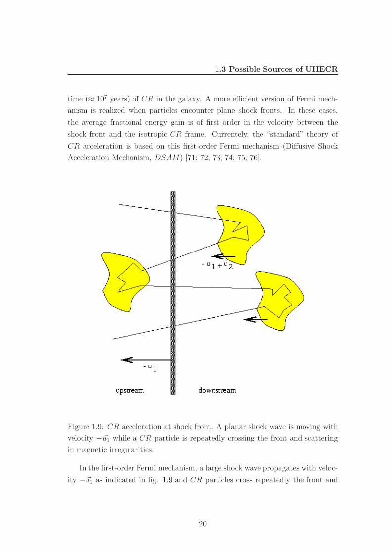
Figure 1.9: CR acceleration at shock front. A planar shock wave is moving with
velocity −u1 while a CR particle is repeatedly crossing the front and scattering
in magnetic irregularities.
In the first-order Fermi mechanism, a large shock wave propagates with veloc-
ity −u1 as indicated in fig. 1.9 and CR particles cross repeatedly the front and
20
1.3 Possible Sources of UHECR
scatter in magnetic irregularities. Relative to the shock front, the downstream
shocked gas is receding with velocity u2, with |u2| < |u1|. In these hypothesys,
before entering in the shock, a CR particle has an energy Ei, a momentum pi and
an incident angle with the shock front propagation direction θi in the laboratory
frame. When the particle crosses the front again, it has energy Ef , momentum
pi and it emerges with an angle θf . In the rest frame of the shock, the particle
has an initial energy
E ′i = γEi(1 − βcosθi) (1.11)
where γ and β are the Lorentz factor and the shock front velocity in units of
speed of light. In the shock frame, there is no change in the energy because all
the scatterings are in the magnetic field, E ′f = E ′
i. In the laboratory frame we
find
Ef = γE ′f (1 + βcosθf) (1.12)
The fractional energy gain in the laboratory frame is then
η =∆E
Ei=
1 − βcosθi + βcosθf − β2cosθicosθf
1 − β2− 1. (1.13)
By considering the rate at which CR cross the shock wave from downstream
to upstream and viceversa, one finds 〈cosθi〉 = 2/3 and 〈cosθf 〉 = −2/3 [75].
Hence the fractional energy gain is
〈η〉 4
3β =
4
3
u1 − u2
c(1.14)
An important feature of diffusive shock acceleration mechanism is that parti-
cles emerge out from the acceleration region with a power-law spectrum, in which
the index depends only on the ratio of the upstream and downstream velocities
(shock compression ratio), not on the shock velocity.
In fact, we can calculate the rate at which CR cross from upstream to down-
stream, given by the projection of the isotropic CR flux onto the plane shock
front
21
1.3 Possible Sources of UHECR
rcross =
∫ 1
0
d(cosθ)
∫ 2π
0
dφnCRv
4πcosθ ≈ nCRv
4(1.15)
where nCR is the density of particles undergoing acceleration. The rate of
convection downstream away from the shock is
rloss = nCRu2. (1.16)
The probability of crossing the shock and escaping is then given by
Prob(escape) =rloss
rcross≈ 4
u2
v(1.17)
and the propability of returning to the shock after crossing upstream to down-
stream is
Prob(return) = 1 − Prob(escape). (1.18)
So the probability to cross n times the shock from downstream to upstream
and viceversa is
Prob(cross ≥ n) = [1 − Prob(escape)]n. (1.19)
Therefore, the energy after n shock crossing is
E = E0
(1 + 〈η〉
)n
(1.20)
where E0 is the initial energy. So the number of particles accelerated to
energies greater than E is
Q(> E) ∝∞∑
m=n
[1 − Prob(escape)]m =[1 − Prob(escape)]n
Prob(escape)(1.21)
This leads to
Q(> E) ∝ 1
Prob(escape)
( E
E0
)−γ
(1.22)
with
γ =ln[1 − Prob(escape)]−1
ln 1 + 〈η〉 (1.23)
22
1.3 Possible Sources of UHECR
1.3.1.4 Top-down acceleration mechanisms
“Top-down” scenarios avoid acceleration problem by assuming that charged and
neutral primaries arise in the decay of supermassive elementary X particles.
Sources of these exotic particles could be:
1. topological defects, from early Universe phase transitions associated with
the spontaneous symmetry breaking [54; 55; 56; 57; 58; 59];
2. long-lived metastable super-heavy relic particles produced through vacuum
fluctuation during the inflationary stage of the Universe [60; 61; 62; 63];
Topological defects (magnetic monopoles, cosmic strings, domain walls, etc.)
are stable and can survive for ever with massive X particles (≈ 1016 − 1019
GeV ) trapped inside them. Sometimes, they can be destroyed through collapse,
annihilation etc., and their energy would be released in the form of massive quanta
that typically decay into quarks and leptons. In a similar way, superheavy relics
could decay in quarks and leptons. Then CR with energies up to mX can be
produced. These topological defects or superheavy particles would lay in the
galactic halo ragion. Another exotic explanation of the UHECR postulates that
relic topological defectes themselves constitute the primaries [64; 65]. General
features of these exotic scenarios are discussed in several reviews [66; 67; 68; 69;
70? ].
1.3.1.5 Cosmic ray Propagation
Looking at the distributions of element abundances (see fig. 1.4) as measured
below the “knee” region, it is evident that cosmic ray abundances are not so
different from those of the Solar System. Main differences are the overabundances
of light elements like lithium, beryllium and boron,and of element just less heavy
then those of the iron group. These differences can be qualitatively accounted
as result of spallation process of primary cosmic rays with interstellar medium
during their travel to the Earth, producing lighter elements.
For the Li − Be − B group it is possible consider the C − N − O group and
its propagation through the interstellar medium. The model is described by
23
1.3 Possible Sources of UHECR
dNp
dX= −Np
λp(1.24)
dNs
dX= −Ns
λs+
NpPsp
λp(1.25)
where Np and Ns are the number of primary particles and secondary ones, X
is the matter quantity (in g/cm2) to pass through, λi are interaction lengths for
different particles, Psp the probability to produce a secondary particle s from a
primary nucleus p, by spallation interactions (Psp = σspallation/σtotal). Solving the
system, one obtains the ratio between primary and secondary abundances, as a
function of X
Ns
Np
=Pspλs
λs − λp
[exp (
Xsp
λp
− Xsp
λs
) − 1]
(1.26)
If we now use the known values for λi and Psp and the measured ratio between
primary group C−N −O and secondary group Li−Be−B, we get that primary
particles should go through 4.3 g/cm2. Hence, with the measured interstellar
medium density, one finds out that primary particles should travel over a distance
of the order of 1 Mpc. So those particles must be confined inside the galaxy for
3 × 10⁶ years.
Generally, propagation mechanism for primary species i can be described
by “Diffusion-Loss Equation” [77], whose solution depends on source contri-
bution and volume in which the species is accelerated. The most simple and
used phenomenological model for the propagation description and for solving the
“Diffusion-Loss Equation” is the “Leaky Box Model”[78]: particles diffuse in a
volume (the galaxy) from which they can escape with a probability function of
the energy. The model predicts different spectral index for different primaries.
In the case of protons, at energies above 4 GeV , one obtains:
Np(E) = Qp(E)τfuga(E) ∝ Qp(E)E−δ (1.27)
with Q(E) primary flux from the sources and δ = 0.6. If we use the known
spectral index (≈ 2.7), it is possible to derive the flux at sources
24
1.4 Experimental Outlook: Extensive Air Showers
Qp(E) ∝ E−γ+δ E−2.1 (1.28)
On the other hand, for iron primaries the flux at sources is
NFe(E) ∝ QFe(E) (1.29)
that is the flux observed has the same spectral index of sources.
The “Leaky Box Model” is able to explain the “knee” feature also, considering
the possibility of particles to leave the galaxy as their energy increases, from
lighter to heavier elements, in agreement with experimental data.
1.4 Experimental Outlook: Extensive Air Show-
ers
For primary cosmic rays with energy above 105 GeV , the flux is so low that the
direct detection is impossible using devices in or above the atmosphere. In such
cases primary particles have enough energy to initiate a cascade whose products
are detectable at ground. These extensive air showers, discovered by Auger and
his group (see sec. 1.1), are used to study cosmic radiation at energies above 105
GeV . The atmosphere is seen as a huge calorimeter, whose properties vary in a
predictable way with altitude and in a relatively unpredictable way with time.
This “calorimeter” provides a vertical thickness of 26 radiation lengths for an
electron and 15 interaction lengths for a proton1.
1.4.1 Shower Development
As long as a primary particle traverses the atmosphere, it dissipates much of
its energy by exiciting and ionizing air molecules along its path, and producing
secondary particles which are able to generate new particles and so on, giving
origin to a cascade. Particle production and the cascade growth continue until
1This is not so different from the number of radiation and interaction lengths at the LHC
detectors. For example, the CMS electromagnetic calorimeter is 25 radiation lengths deepand the hadron calorimeter constitutes 11 interaction lengths.
25
1.4 Experimental Outlook: Extensive Air Showers
the average energy lost by ionization by secondary particles becomes of the same
order of the average energy needed to produce a new particle generation. At
this point, the shower reaches its maximum development and from now on the
number of particles produced at each generation decreases down to zero.
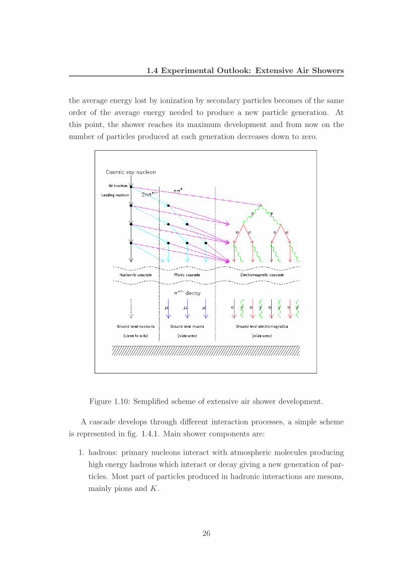
Figure 1.10: Semplified scheme of extensive air shower development.
A cascade develops through different interaction processes, a simple scheme
is represented in fig. 1.4.1. Main shower components are:
1. hadrons: primary nucleons interact with atmospheric molecules producing
high energy hadrons which interact or decay giving a new generation of par-
ticles. Most part of particles produced in hadronic interactions are mesons,
mainly pions and K.
26
1.4 Experimental Outlook: Extensive Air Showers
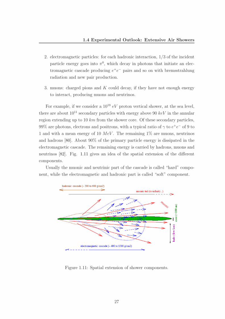
2. electromagnetic particles: for each hadronic interaction, 1/3 of the incident
particle energy goes into π0, which decay in photons that initiate an elec-
tromagnetic cascade producing e+e− pairs and so on with bremsstrahlung
radiation and new pair production.
3. muons: charged pions and K could decay, if they have not enough energy
to interact, producing muons and neutrinos.
For example, if we consider a 1019 eV proton vertical shower, at the sea level,
there are about 1011 secondary particles with energy above 90 keV in the annular
region extending up to 10 km from the shower core. Of these secondary particles,
99% are photons, electrons and positrons, with a typical ratio of γ to e+e− of 9 to
1 and with a mean energy of 10 MeV . The remaining 1% are muons, neutrinos
and hadrons [80]. About 90% of the primary particle energy is dissipated in the
electromagnetic cascade. The remaining energy is carried by hadrons, muons and
neutrinos [82]. Fig. 1.11 gives an idea of the spatial extension of the different
components.
Usually the muonic and neutrinic part of the cascade is called “hard” compo-
nent, while the electromagnetic and hadronic part is called “soft” component.
Figure 1.11: Spatial extension of shower components.
27
1.4 Experimental Outlook: Extensive Air Showers
The evolution of an EAS is dominated by electromagnetic processes. Photons-
induced showers are even more dominated by electromagnetic channel, as the only
significant muon generation mechanism is the decay of charged pions and kaons
produced in γ−air interactions [83].
The cascade shows a conical form around primary trajectory (“leading particle
effect”), and this trajectory is called “shower axis”. The impact point of the
shower axis on the ground is called “shower core”. The shower reaches the ground
in the form of a giant “saucer” travelling nearly at the speed of light.
To describe an atmospheric cascade one usually defines the following quanti-
ties:
1. N(X), the longitudinal profile, i.e. the number of particles of the shower
(shower size) as a function of the traversed atmospheric depth X;
2. Xmax (measuredin g/cm2), the slanth depth at which the EAS reaches its
maximum, the maximum size Nmax;
3. ρ(r), the particle density at distance r from shower axis, in the plane per-
pendicular to the axis, the lateral distribution.
Longitudinal development, Xmax and lateral distribution depend on the pri-
mary energy and composition. It is not possible to measure the lateral distribu-
tion at different depths, experiments can only measure it at one depth and usually
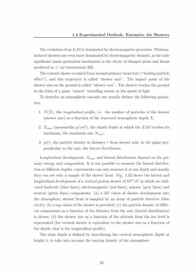
they can see only a sample of the shower front. Fig. 1.12 shows the lateral and
longitudinal development of a vertical proton shower of 1014 eV in which are indi-
cated hadronic (blue lines), electromagnetic (red lines), muonic (grey lines) and
neutral (green lines) components: (a) a 3D vision of shower development into
the atmosphere, shower front is sampled by an array of particle detector (blue
circle); (b) a top vision of the shower is provided; (c) the particle density of differ-
ent components as a function of the distance from the axis (lateral distribution)
is shown; (d) the shower size as a function of the altitude from the sea level is
represented (for vertical shower is equivalent to the shower size as a function of
the depth, that is the longitudinal profile).
The slant depth is defined by introducing the vertical atmospheric depth at
height h, to take into account the varying density of the atmosphere
28
1.4 Experimental Outlook: Extensive Air Showers
Figure 1.12: Lateral and longitudinal development of a vertical proton shower of
1014 eV , hadronic (blue lines), electromagnetic (red lines), muonic (grey lines)
and neutral (green lines) components are indicated; (a) a 3D vision of shower
development into the atmosphere is presented, shower front is sampled by an
array of particle detector (blue circle); (b) a top vision of the shower is provided;
(c) it is shown the particle density of different components as a function of the
distance from the axis (lateral distribution); (d) it is represented the shower size
as a function of the altitude from the sea level (for vertical showers is equivalent
to the shower size as a function of the depth, i.e. the longitudinal profile).
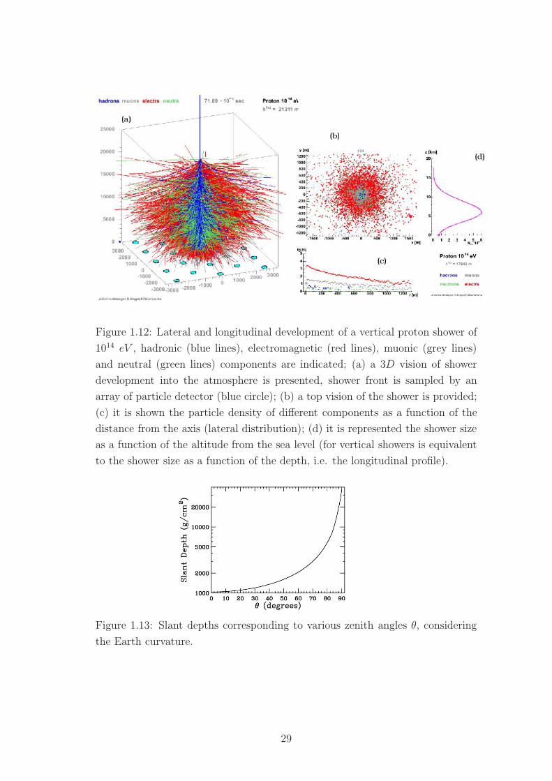
Figure 1.13: Slant depths corresponding to various zenith angles θ, considering
the Earth curvature.
29
1.4 Experimental Outlook: Extensive Air Showers
Xv(h) =
∫ infty
h
ρatm(z)dz (1.30)
where the integration is done over the altitude, z, and ρatm is the atmospheric
density. The slant depth for a shower is then the same integral performed along
particle trajectory. Fig. 1.13 shows the variation of the slant depth with zenith
angle of the trajectory. Neglecting Earth curvature, we can use the approximation
X = Xv(h)/cosθ, where θ is the zenith angle of the primary particle cosmic
ray. The error associated with this approximation is less than 4% for θ 80.
The vertical atmosphere is ≈ 1000 g/cm2 and it is about 36 times deeper for
completely horizontal showers.
1.4.1.1 The Electromagnetic Component
The electromagnetic part of a cascade typically origins by π0 decay
π0 → γ + γ (1.31)
other possible decays, π0 → γ + e+ + e− and π0 → e+ + e− + e+ + e−, are
negligible [81].
Then, the produced photons initiate the cascade, they convert into e+e− pair,
which in turn emit synchrotron photons and so on.
Particle production slows down at a critical energy EC , defined 1 as the en-
ergy at which ionization loss is equal to the breemsstrahlung loss for an electron
(positron). That leads to EC = 710MeV/(Zeff + 0.92) ≈ 86 MeV 2 [87]. At crit-
ical energy ionization loss take over from breemsstrahlung and pair production
as the dominant energy loss mechanism. The changeover from radiation and pair
production losses to ionization losses depopulates the shower.
It is then possible to categorize the shower development in three phases: the
growth phase, in which all particle have energy > EC ; the shower maximum; the
shower tail, where particles only lose energy, get absorbed or decay.
1Several different definitions of the critical energy appear in the literature [86]2For altitude up to 90 km above sea level, the air is a mixture of 78.09% of N2, 20.95%
of O2 and 0.96% of other gases [88]. Such a mixture is generally modeled as an homogeneussubstance with atomic charge Zeff = 7.3 and mass number Aeff = 14.6.
30
1.4 Experimental Outlook: Extensive Air Showers
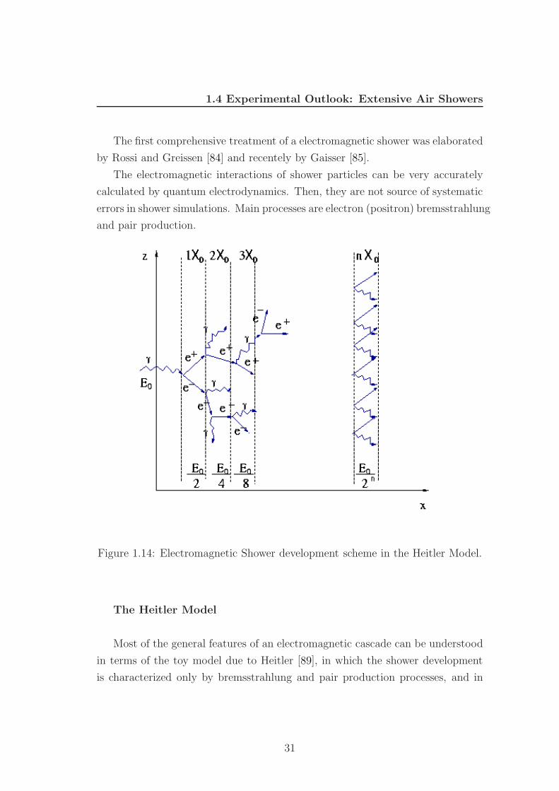
The first comprehensive treatment of a electromagnetic shower was elaborated
by Rossi and Greissen [84] and recentely by Gaisser [85].
The electromagnetic interactions of shower particles can be very accurately
calculated by quantum electrodynamics. Then, they are not source of systematic
errors in shower simulations. Main processes are electron (positron) bremsstrahlung
and pair production.
Figure 1.14: Electromagnetic Shower development scheme in the Heitler Model.
The Heitler Model
Most of the general features of an electromagnetic cascade can be understood
in terms of the toy model due to Heitler [89], in which the shower development
is characterized only by bremsstrahlung and pair production processes, and in
31
1.4 Experimental Outlook: Extensive Air Showers
which each interaction process produces the conversion of one particle in two.
These processes have the same interaction lenght X0. Hence, the model assumes:
1. in the bremsstrahlung process, final photon and electron (positron) share
the energy of the initial electron (positron);
2. in the pair production process, e+ and e− share the energy of the initial
photon;
3. multiple scattering is neglected and the shower development is unidimen-
sional;
4. Compton scattering is neglected.
In the model, the shower is represented as a tree with branches that bifur-
cate every X0, until they fall below the critical energy (see fig. 1.14). Above
EC , the number of particles grows geometrically, so after n (n = X/X0) steps
(branchings), the total number of particles as a function of the slant depth is
N(X) = 2X/X0 (1.32)
while the energy for each particle is
E(X) =E0
N(X)(1.33)
where E0 is the energy of the particle that initiated the shower (the first
photon). At the maximum, the number of particles should be
N(Xmax) =E0
Ec(1.34)
then we get
Xmax =X0 ln(E0/EC)
ln 2(1.35)
In the real life, high energy photons, electrons and positrons, below 1010 GeV ,
have mean interaction lengths of 37 g/cm2, whereas above this critical energy the
competing LPM [79] and geomagnetic effects lead to interaction lengths between
32
1.4 Experimental Outlook: Extensive Air Showers
45 and 60 g/cm2 [80]. LPM and geomagnetic effects introduce large fluctuations
in the value of Xmax for photon-induced shower. Nevertheless, the toy model
prediction lies within the range of these fluctuations.
The Heitler model is enlightening for barion-induced shower also. In particu-
lar, for proton showers, the model predicts that Xmax scales logarithmically with
the primary energy, while Nmax scales linearly. In the case of heavy nuclei, us-
ing the superposition principle as reasonable approximation, a shower produced
by nucleus with energy EA and mass A, is modeled by a collection of A proton
shower. Then its maximum is Xmax ∝ ln(E0/A).
The Heitler model, though very simple, is very useful to get a first intuition
about global shower properties, anyway, the details of shower evolution are too
complicated to be described by such a simple analytical model.
To obtain a more precise analytical treatment, the use of diffusion equations
is required. Their solutions are [84]
nedE =dE
Es+1(a1e
λ1(s)t + a2eλ2(s)t) (1.36)
nγdE =dE
Es+1(
a1c
λpair + λ1(s)eλ1(s)t +
a2c
λpair + λ2(s)eλ2(s)t) (1.37)
where nedE and nγdE are the number of electrons (positrons) and photons
with energy between E and E + dE, t is the slant depth traversed in radiation
lenghts (i.e. t = X/X0), λpair is the interaction length for pair production and
λ1(s) and λ2(s) are two functions of the parameter s, called “shower age”. The
shower age is lower than one in the growth phase (“young shower”), is equal
to one at the maximum and is greater than one in the shower tail phase (“old
shower”). For a quantitative analysis ionization loss processes are required. It
is needed to consider the transport equations in air for electrons (positrons) and
photons [85], whose solutions have been obtained by Snyder, Scott [90; 91] and
Greisen [92]. For a large number of particles, these solutions could be expressed
using the Snyder-Scott-Greisen parametrization
N(E0, t) =0.31
[ln(E0/Ec)]1/2exp (t(1 − 1.5 ln s)) (1.38)
where
33
1.4 Experimental Outlook: Extensive Air Showers
s =3t
t + 2 ln(E0/Ec)(1.39)
The total electron number on the total track length is given by
∫ ∞
0
N(E0, t)dt =E0
Ec
(1.40)
considering constant the energy loss rate by ionization processes. These solu-
tions provide a good description of the longitudinal profile (number of particles
as a function of the depth) of a shower. Neverthless, neglecting processes as
Compton scattering, photoelectric effect and electron-positron annihilation, an
uncorrect estimation of the number of low energy electrons is obtained.
Full Monte Carlo simulation of interaction and transport of each individual
particle would be required to get a complete and precise modeling of the shower
development.
1.4.1.2 The Muon Component
The muon content of a shower is an important feature. It differs from electro-
magnetic component for two main reasons:
1. muons are generated through the decay of cooled charged pions (Eπ± 1
TeV ) and thus the muon content is sensitive to the initial baryonic nature
of the primary. Furthermore, there is no “muonic cascade” so the number
of muons at ground level is much smaller than the number of electrons.
2. muons have a much smaller cross section for radiation and pair production
and so the muonic component develops separately and differently than the
electronic component does.
The ratio of electrons to muons depends strongly on the distance from the
core: for a vertical 1019 eV proton it varies from 17 to 1 at 200 m from the core
to 1 to 1 at 2000 m. The ratio depends also on the inclination. At the zenith
angles greater than 60 the ratio is constant. As the zenith angle grows, the ratio
decreases, until θ = 75, it is 400 times smaller than for a vertical shower. Even
the average muon energy depends on the zenith angle. For horizontal showers,
34
1.4 Experimental Outlook: Extensive Air Showers
low energy muons are filtered out so the average muon energy is two order of
magnitude greater than for vertical shower. It should be noted that the curvature
of the muon distribution could serve as a discriminator between hadronic models
[113].
High energy muons lose energy through pair production, muon-nucleus inter-
action, bremsstrahlung and knock-on electron (δ− ray) production [114]. The δ−ray production has a short mean free path and a small inelasticity, so it could be
seen as a continuous process. Main energy loss mechanisms are pair production
and bremsstrahlung. Energy loss by pair production is slitghtly more important
than bremsstrahlung at about 1 GeV and becomes increasingly dominant with
the energy.
1.4.1.3 The Hadron Component
Hadronic interactions at ultra high energies constitute one of the most problem-
atic sources of systematic error in the air shower analysis.
The highest primary energy measured thus far is ≈ 1020.5 eV , corresponding to
a nucleon-nucleon center of mass energy√
s ≈ 1014.9 eV/√
A, where A is the mass
number of the primary particle. Hence, ultra high energy cosmic ray interaction
are orders of magnitude beyond the energy range achieveble by present and future
collider experiments.
The typical characteristic of most hadronic interactions occuring in a shower
development is the soft multiparticle production with a small transverse momenta
with respect to the collision axis. Despite the fact that calculations based on ordi-
nary perturbative QCD are not feasible, there are some phenomenological models
that successfully take into account the main properties of the soft diffractive pro-
cesses. These models, inspired by 1/N QCD expansion, are also supplemented
with general theoretical principles like duality, unitarity, Regge behavior and par-
ton structure. Interactions are described by highly complicated modes, known as
Reggeons. Up to 50 GeV , the slow growth of the cross section with√
s is driven
by a dominant contribution of a special Reggeon, the Pomeron. In the energy
range in which we are interested in, semihard interactions arising from the hard
scattering of partons that carry only a very small fraction of the momenta of their
35
1.4 Experimental Outlook: Extensive Air Showers
parent hadrons can also compete with soft processes. Unlike soft processes, this
semihard physics can be computed in perturbative QCD.
For semplicity, we will follow the example of a proton hitting the atmosphere.
By means of ionization loss processes, a high energy proton has a energy loss
rate in air of 2 MeV/(g/cm2). A visible modification of its motion occurs when
the proton interacts with an atmospheric nucleus. Supposing that the proton
interacts with just a nucleon of the target nucleus, we get the reaction
p + p → p + p + N (π0 + π+ + π−) (1.41)
in which contribution from K, Λ, η, Ω, Σ ... are neglected. A possible
estimation of the number of secondary particles is ns = 2.5E0.25 [115]1.
In such a process, the produced particles carry away about one half of the
primary energy 2. The energy is shared among pions, so at each generation, on
average 1/3 of the energy is carried by π0 and 2/3 by π±. Usually, neutral pions
feed the electromagnetic component of the shower, while charged pions are able to
interact producing a new hadron generation. As for the electromagnetic cascade,
generation by generation, the average energy of generated particles decreases and
the growth of the shower slows down. When the decay or the absorbtion is
competitive with interaction and particle production processes, the cascade goes
to die out.
The hadronic component develops very close to the shower axis. The pions
are emitted forward and backward within a cone which aperture is related to the
energy by [93; 94]
E =2 mπ c2
tg2 η(1.42)
where mπ is the pion mass in the rest frame and η is the angular aperture.
At higher energies it is possible to obtain3
1 There are still a lot of discussion about the estimation of the particle multiplicity.2 As well as the particle multiplicity, the inelasticity is still affected by uncertainties due to
the use of just phenomenological models3If E > 1012 eV then η < 1
36
1.4 Experimental Outlook: Extensive Air Showers
η = (2 mπc
2
E)1/2 ≈
√2
E(1.43)
with E expressed in GeV units. The muon component derives from the decay
of charged pions. The 75% reaches the ground.
In the case of heavy nuclei of mass A and energy E, we can use the approx-
imation of the superposition model and imagine the shower as a collection of A
proton showers with energy E/A. As already seen, from the Heitler model one
derives that the maximum depth is Xmax ∝ ln(E0/A). In principle, it should be
possible to distinguish primary particles looking at the Xmax.
An important feature of a heavy primary shower is the lower fluctuation of
the longitudinal profile with respect to a proton shower one, because the obtained
profile for a primary of mass A is an average over A proton profiles. An additional
difference with respect to the proton case is the muon population. It is possible
to see that the number of muon produced by a primary of mass A and energy E
is [85]
NAµ ∝ A(E/A)0.85 (1.44)
that can be also expressed as a function of the number of muon produced by
proton shower
NAµ = A0.15Np
µ (1.45)
Hence, an iron nucleus will produce a number of muons 80% greater than that
produced by a proton.
So far it seem that it is possible to distinguish, in principle, light primaries
(protons) from heavy primaries (irons) using the Xmax and the muon population.
1.4.2 The Longitudinal Development
The longitudinal development for a given primary particle of a given energy de-
pends only on the cumulated slant depth X (the thickness of air already crossed).
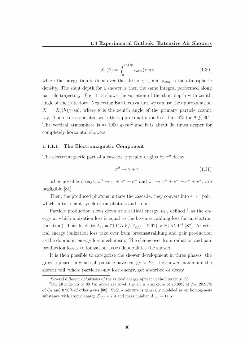
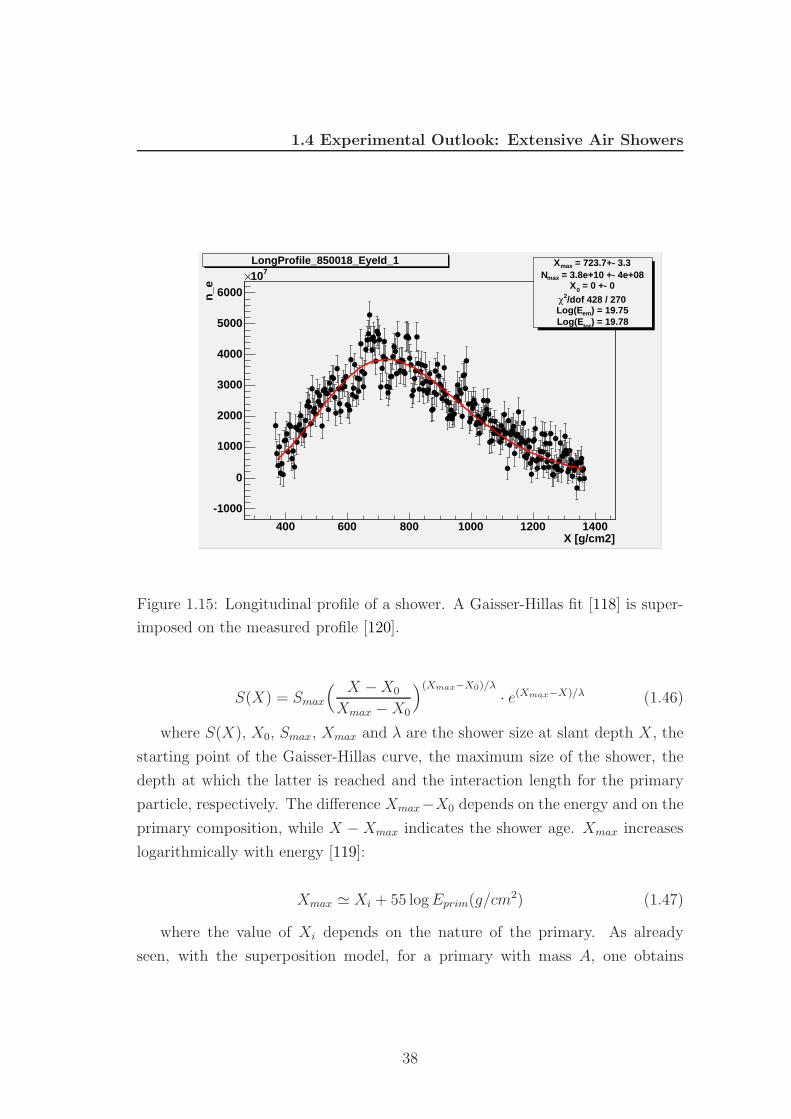
Fig. 1.15 shows the longitudinal profile of a shower measured at the Auger Ob-
servatory.
Experimental points are fitted by the Gaisser-Hillas function [118]:
37
1.4 Experimental Outlook: Extensive Air Showers
X [g/cm2]400 600 800 1000 1200 1400
n_e
-1000
0
1000
2000
3000
4000
5000
6000
710× = 723.7+- 3.3maxX
= 3.8e+10 +- 4e+08maxN = 0 +- 00X
/dof 428 / 2702χ) = 19.75emLog(E) = 19.78totLog(E
LongProfile_850018_EyeId_1
Figure 1.15: Longitudinal profile of a shower. A Gaisser-Hillas fit [118] is super-
imposed on the measured profile [120].
S(X) = Smax
( X − X0
Xmax − X0
)(Xmax−X0)/λ
· e(Xmax−X)/λ (1.46)
where S(X), X0, Smax, Xmax and λ are the shower size at slant depth X, the
starting point of the Gaisser-Hillas curve, the maximum size of the shower, the
depth at which the latter is reached and the interaction length for the primary
particle, respectively. The difference Xmax−X0 depends on the energy and on the
primary composition, while X − Xmax indicates the shower age. Xmax increases
logarithmically with energy [119]:
Xmax Xi + 55 log Eprim(g/cm2) (1.47)
where the value of Xi depends on the nature of the primary. As already
seen, with the superposition model, for a primary with mass A, one obtains
38
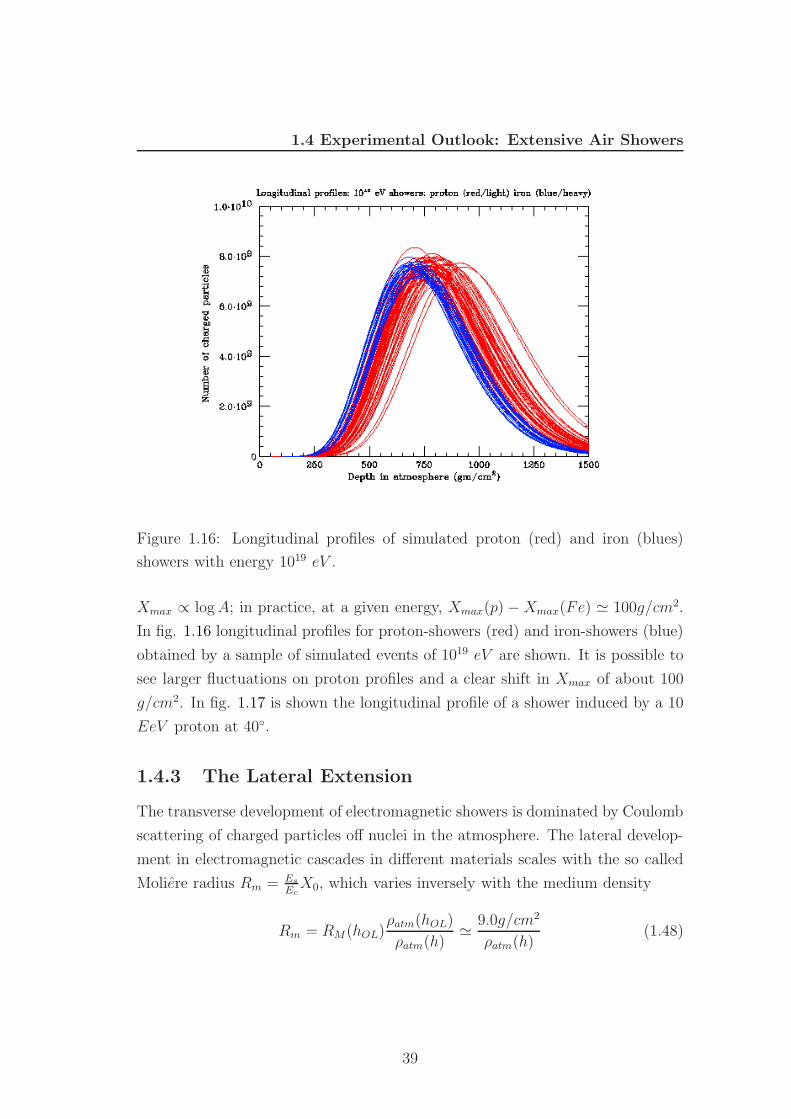
1.4 Experimental Outlook: Extensive Air Showers
Figure 1.16: Longitudinal profiles of simulated proton (red) and iron (blues)
showers with energy 1019 eV .
Xmax ∝ log A; in practice, at a given energy, Xmax(p) − Xmax(Fe) 100g/cm2.
In fig. 1.16 longitudinal profiles for proton-showers (red) and iron-showers (blue)
obtained by a sample of simulated events of 1019 eV are shown. It is possible to
see larger fluctuations on proton profiles and a clear shift in Xmax of about 100
g/cm2. In fig. 1.17 is shown the longitudinal profile of a shower induced by a 10
EeV proton at 40.
1.4.3 The Lateral Extension
The transverse development of electromagnetic showers is dominated by Coulomb
scattering of charged particles off nuclei in the atmosphere. The lateral develop-
ment in electromagnetic cascades in different materials scales with the so called
Moliere radius Rm = Es
EcX0, which varies inversely with the medium density
Rm = RM(hOL)ρatm(hOL)
ρatm(h) 9.0g/cm2
ρatm(h)(1.48)
39
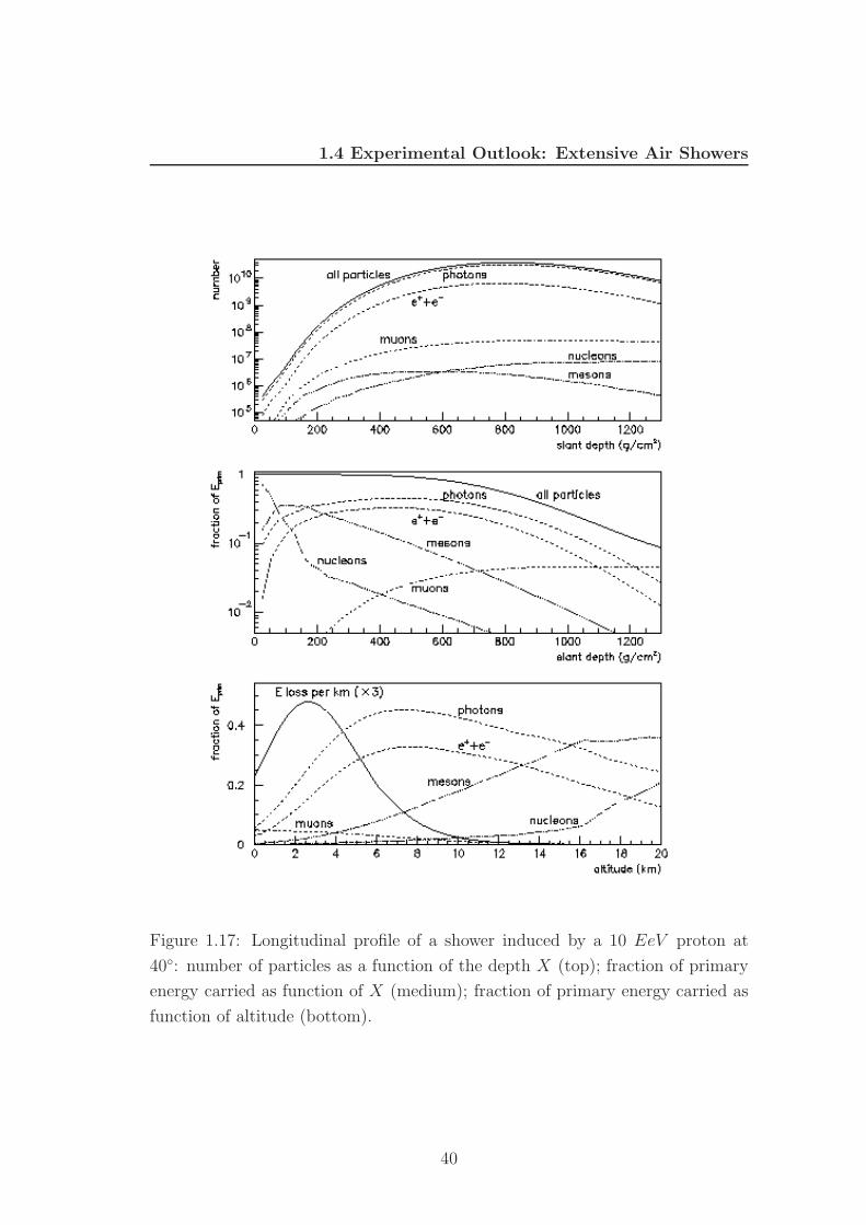
1.4 Experimental Outlook: Extensive Air Showers
Figure 1.17: Longitudinal profile of a shower induced by a 10 EeV proton at
40: number of particles as a function of the depth X (top); fraction of primary
energy carried as function of X (medium); fraction of primary energy carried as
function of altitude (bottom).
40
1.4 Experimental Outlook: Extensive Air Showers
where Es = mec2(4π/α)1/2 21 MeV [86], EC the critical energy and X0 the
electron interaction lenght in air, ρatm is the atmospheric density and the subscript
OL indicates a quantity taken at a given observation level.
A Very detailed 3D integration of cascade equations has been performed by
Nishimura and Kamata [96; 97] and later worked out by Greisen [95]. They
derived the well-known NKG formula to describe the lateral structure function
for a pure electromagnetic shower
ρ(r) =Ne
R2M
C(s)(r
Rm
)s−2(r
Rm
+ 1)s−4.5 (1.49)
where Ne is the total number of electrons, r is the distance from the shower
axis and
C(s) =Γ(4.5 − s)
2πΓ(s)Γ(4.5 − 2s)(1.50)
The NKG could be extended to describe the electromagnetic component of
barion-induced showers [98]. In such an extension, a deviation of behavior of
Moliere radius is founded, by using the age parameter defined for pure electro-
magnetic cascades. The NKG is generalized changing the definition of the age
parameter in
s = 3(1 +
2β
t
)−1
(1.51)
where the β parameter takes into account the deviations from he theoretical
value.
The modified NKG formula provides a good description of the e+e− lateral
distribution at all stages of the shower development for values of r sufficientely
far from the hadronic core, that is in the interesting region (typical ground array
can only measure densities at r > 100 m from the core, where detectors are not
saturated.
In the case of inclined showers, one usually analyzes particle densities in the
plane perpendicular to the shower axis. But additional asimmetry and geometri-
cal effects are introduced [98; 109]. A lateral distribution function (LDF ) valid
at all zenith angles θ < 70 can be determined by considering
41
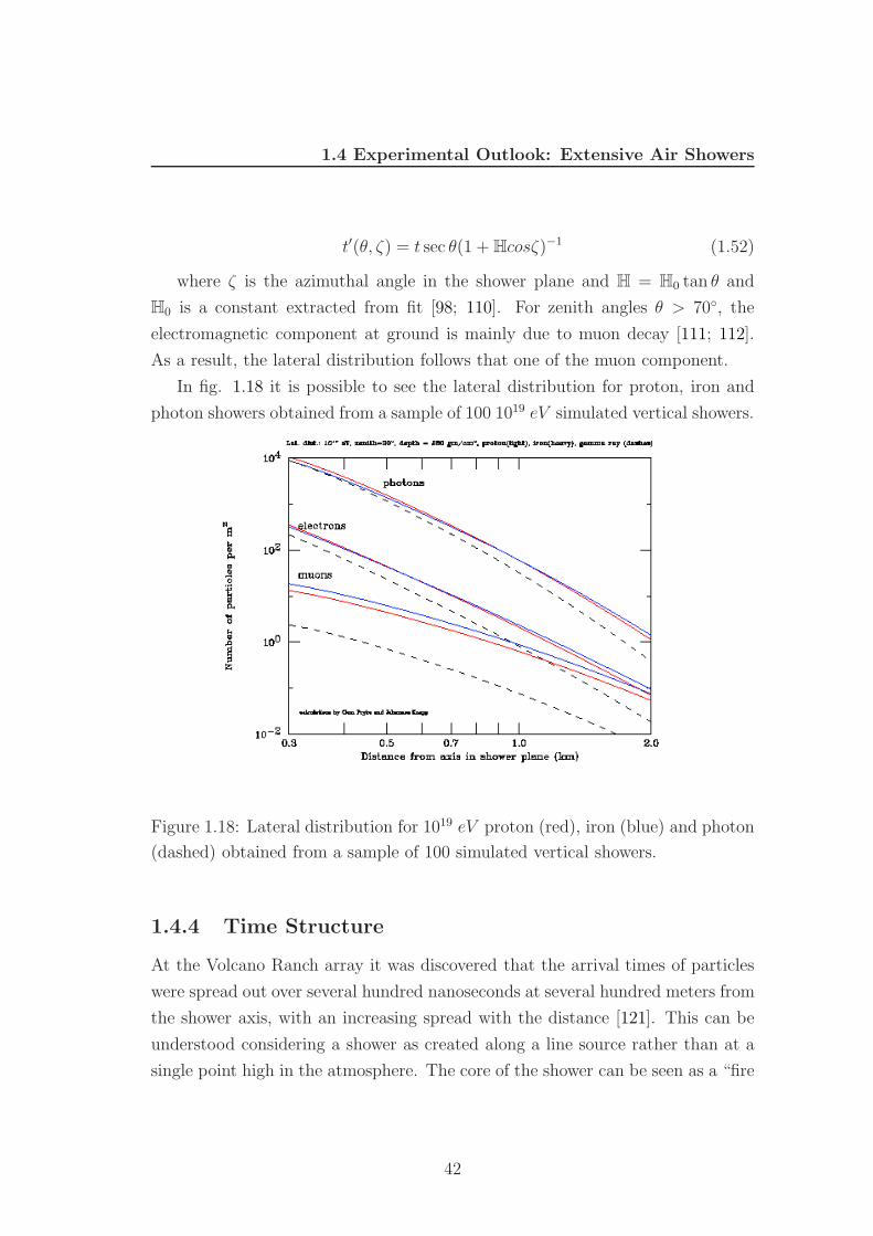
1.4 Experimental Outlook: Extensive Air Showers
t′(θ, ζ) = t sec θ(1 + Hcosζ)−1 (1.52)
where ζ is the azimuthal angle in the shower plane and H = H0 tan θ and
H0 is a constant extracted from fit [98; 110]. For zenith angles θ > 70, the
electromagnetic component at ground is mainly due to muon decay [111; 112].
As a result, the lateral distribution follows that one of the muon component.
In fig. 1.18 it is possible to see the lateral distribution for proton, iron and
photon showers obtained from a sample of 100 1019 eV simulated vertical showers.
Figure 1.18: Lateral distribution for 1019 eV proton (red), iron (blue) and photon
(dashed) obtained from a sample of 100 simulated vertical showers.
1.4.4 Time Structure
At the Volcano Ranch array it was discovered that the arrival times of particles
were spread out over several hundred nanoseconds at several hundred meters from
the shower axis, with an increasing spread with the distance [121]. This can be
understood considering a shower as created along a line source rather than at a
single point high in the atmosphere. The core of the shower can be seen as a “fire
42
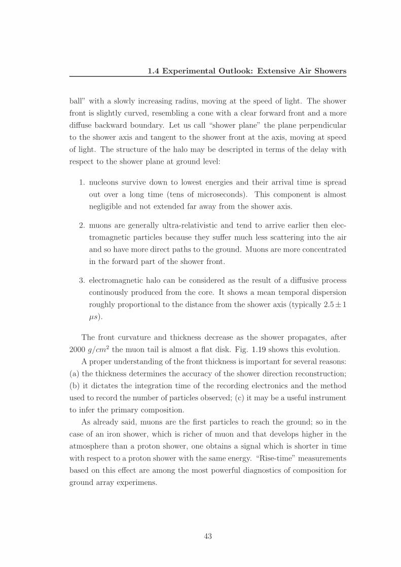
1.4 Experimental Outlook: Extensive Air Showers
ball” with a slowly increasing radius, moving at the speed of light. The shower
front is slightly curved, resembling a cone with a clear forward front and a more
diffuse backward boundary. Let us call “shower plane” the plane perpendicular
to the shower axis and tangent to the shower front at the axis, moving at speed
of light. The structure of the halo may be descripted in terms of the delay with
respect to the shower plane at ground level:
1. nucleons survive down to lowest energies and their arrival time is spread
out over a long time (tens of microseconds). This component is almost
negligible and not extended far away from the shower axis.
2. muons are generally ultra-relativistic and tend to arrive earlier then elec-
tromagnetic particles because they suffer much less scattering into the air
and so have more direct paths to the ground. Muons are more concentrated
in the forward part of the shower front.
3. electromagnetic halo can be considered as the result of a diffusive process
continously produced from the core. It shows a mean temporal dispersion
roughly proportional to the distance from the shower axis (typically 2.5±1
µs).
The front curvature and thickness decrease as the shower propagates, after
2000 g/cm2 the muon tail is almost a flat disk. Fig. 1.19 shows this evolution.
A proper understanding of the front thickness is important for several reasons:
(a) the thickness determines the accuracy of the shower direction reconstruction;
(b) it dictates the integration time of the recording electronics and the method
used to record the number of particles observed; (c) it may be a useful instrument
to infer the primary composition.
As already said, muons are the first particles to reach the ground; so in the
case of an iron shower, which is richer of muon and that develops higher in the
atmosphere than a proton shower, one obtains a signal which is shorter in time
with respect to a proton shower with the same energy. “Rise-time” measurements
based on this effect are among the most powerful diagnostics of composition for
ground array experimens.
43
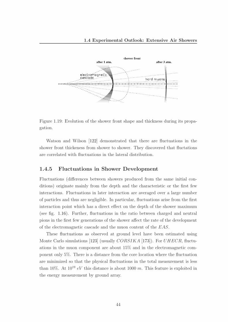
1.4 Experimental Outlook: Extensive Air Showers
Figure 1.19: Evolution of the shower front shape and thickness during its propa-
gation.
Watson and Wilson [122] demonstrated that there are fluctuations in the
shower front thickeness from shower to shower. They discovered that fluctations
are correlated with fluctuations in the lateral distribution.
1.4.5 Fluctuations in Shower Development
Fluctuations (differences between showers produced from the same initial con-
ditions) originate mainly from the depth and the characteristic or the first few
interactions. Fluctuations in later interaction are averaged over a large number
of particles and thus are negligible. In particular, fluctuations arise from the first
interaction point which has a direct effect on the depth of the shower maximum
(see fig. 1.16). Further, fluctuations in the ratio between charged and neutral
pions in the first few generations of the shower affect the rate of the development
of the electromagnetic cascade and the muon content of the EAS.
These fluctuations as observed at ground level have been estimated using
Monte Carlo simulations [123] (usually CORSIKA [173]). For UHECR, fluctu-
ations in the muon component are about 15% and in the electromagnetic com-
ponent only 5%. There is a distance from the core location where the fluctuation
are minimized so that the physical fluctuations in the total measurement is less
than 10%. At 1019 eV this distance is about 1000 m. This feature is exploited in
the energy measurement by ground array.
44
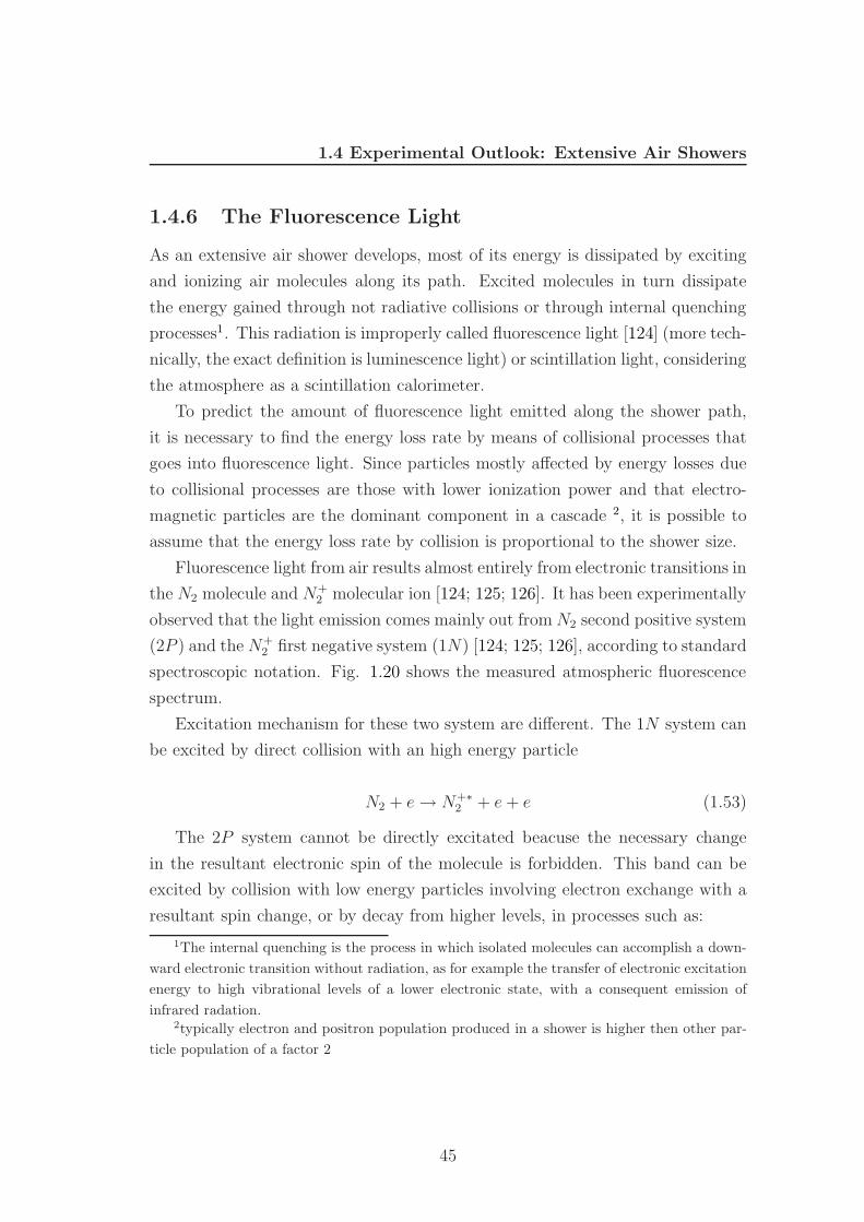
1.4 Experimental Outlook: Extensive Air Showers
1.4.6 The Fluorescence Light
As an extensive air shower develops, most of its energy is dissipated by exciting
and ionizing air molecules along its path. Excited molecules in turn dissipate
the energy gained through not radiative collisions or through internal quenching
processes1. This radiation is improperly called fluorescence light [124] (more tech-
nically, the exact definition is luminescence light) or scintillation light, considering
the atmosphere as a scintillation calorimeter.
To predict the amount of fluorescence light emitted along the shower path,
it is necessary to find the energy loss rate by means of collisional processes that
goes into fluorescence light. Since particles mostly affected by energy losses due
to collisional processes are those with lower ionization power and that electro-
magnetic particles are the dominant component in a cascade 2, it is possible to
assume that the energy loss rate by collision is proportional to the shower size.
Fluorescence light from air results almost entirely from electronic transitions in
the N2 molecule and N+2 molecular ion [124; 125; 126]. It has been experimentally
observed that the light emission comes mainly out from N2 second positive system
(2P ) and the N+2 first negative system (1N) [124; 125; 126], according to standard
spectroscopic notation. Fig. 1.20 shows the measured atmospheric fluorescence
spectrum.
Excitation mechanism for these two system are different. The 1N system can
be excited by direct collision with an high energy particle
N2 + e → N+∗2 + e + e (1.53)
The 2P system cannot be directly excitated beacuse the necessary change
in the resultant electronic spin of the molecule is forbidden. This band can be
excited by collision with low energy particles involving electron exchange with a
resultant spin change, or by decay from higher levels, in processes such as:
1The internal quenching is the process in which isolated molecules can accomplish a down-ward electronic transition without radiation, as for example the transfer of electronic excitationenergy to high vibrational levels of a lower electronic state, with a consequent emission ofinfrared radation.
2typically electron and positron population produced in a shower is higher then other par-ticle population of a factor 2
45
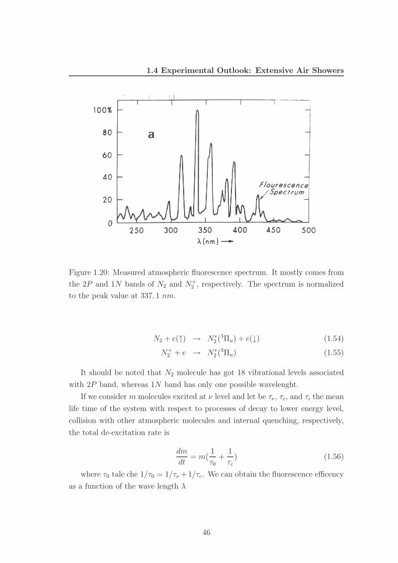
1.4 Experimental Outlook: Extensive Air Showers
Figure 1.20: Measured atmospheric fluorescence spectrum. It mostly comes from
the 2P and 1N bands of N2 and N+2 , respectively. The spectrum is normalized
to the peak value at 337, 1 nm.
N2 + e(↑) → N∗2 (3Πu) + e(↓) (1.54)
N+2 + e → N∗
2 (3Πu) (1.55)
It should be noted that N2 molecule has got 18 vibrational levels associated
with 2P band, whereas 1N band has only one possible wavelenght.
If we consider m molecules excited at ν level and let be τν , τc, and τi the mean
life time of the system with respect to processes of decay to lower energy level,
collision with other atmospheric molecules and internal quenching, respectively,
the total de-excitation rate is
dm
dt= m(
1
τ0+
1
τc) (1.56)
where τ0 tale che 1/τ0 = 1/τν +1/τc. We can obtain the fluorescence efficency
as a function of the wave length λ
46
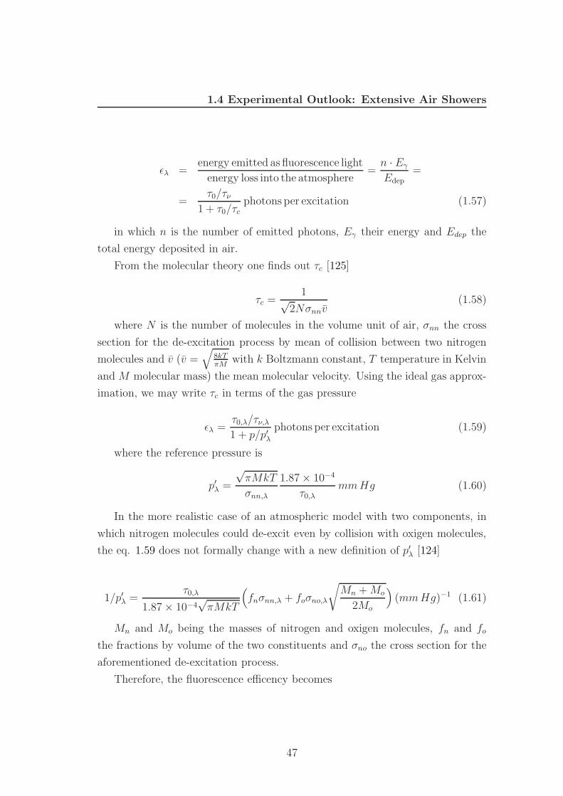
1.4 Experimental Outlook: Extensive Air Showers
ελ =energy emitted as fluorescence light
energy loss into the atmosphere=
n · Eγ
Edep=
=τ0/τν
1 + τ0/τc
photons per excitation (1.57)
in which n is the number of emitted photons, Eγ their energy and Edep the
total energy deposited in air.
From the molecular theory one finds out τc [125]
τc =1√
2Nσnnv(1.58)
where N is the number of molecules in the volume unit of air, σnn the cross
section for the de-excitation process by mean of collision between two nitrogen
molecules and v (v =√
8kTπM
with k Boltzmann constant, T temperature in Kelvin
and M molecular mass) the mean molecular velocity. Using the ideal gas approx-
imation, we may write τc in terms of the gas pressure
ελ =τ0,λ/τν,λ
1 + p/p′λphotons per excitation (1.59)
where the reference pressure is
p′λ =
√πMkT
σnn,λ
1.87 × 10⁻⁴
τ0,λmm Hg (1.60)
In the more realistic case of an atmospheric model with two components, in
which nitrogen molecules could de-excit even by collision with oxigen molecules,
the eq. 1.59 does not formally change with a new definition of p′λ [124]
1/p′λ =τ0,λ
1.87 × 10⁻⁴√
πMkT
(fnσnn,λ + foσno,λ
√Mn + Mo
2Mo
)(mm Hg)−1 (1.61)
Mn and Mo being the masses of nitrogen and oxigen molecules, fn and fo
the fractions by volume of the two constituents and σno the cross section for the
aforementioned de-excitation process.
Therefore, the fluorescence efficency becomes
47
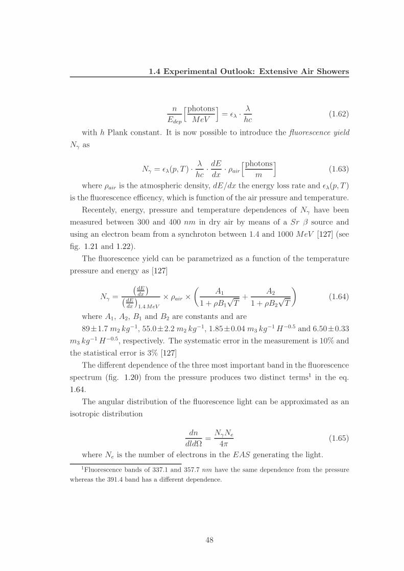
1.4 Experimental Outlook: Extensive Air Showers
n
Edep
[photons
MeV
]= ελ · λ
hc(1.62)
with h Plank constant. It is now possible to introduce the fluorescence yield
Nγ as
Nγ = ελ(p, T ) · λ
hc· dE
dx· ρair
[photons
m
](1.63)
where ρair is the atmospheric density, dE/dx the energy loss rate and ελ(p, T )
is the fluorescence efficency, which is function of the air pressure and temperature.
Recentely, energy, pressure and temperature dependences of Nγ have been
measured between 300 and 400 nm in dry air by means of a Sr β source and
using an electron beam from a synchroton between 1.4 and 1000 MeV [127] (see
fig. 1.21 and 1.22).
The fluorescence yield can be parametrized as a function of the temperature
pressure and energy as [127]
Nγ =
(dEdx
)(
dEdx
)1.4 MeV
× ρair ×(
A1
1 + ρB1
√T
+A2
1 + ρB2
√T
)(1.64)
where A1, A2, B1 and B2 are constants and are
89±1.7 m2 kg−1, 55.0±2.2 m2 kg−1, 1.85±0.04 m3 kg−1 H−0.5 and 6.50±0.33
m3 kg−1 H−0.5, respectively. The systematic error in the measurement is 10% and
the statistical error is 3% [127]
The different dependence of the three most important band in the fluorescence
spectrum (fig. 1.20) from the pressure produces two distinct terms1 in the eq.
1.64.
The angular distribution of the fluorescence light can be approximated as an
isotropic distribution
dn
dldΩ=
NγNe
4π(1.65)
where Ne is the number of electrons in the EAS generating the light.
1Fluorescence bands of 337.1 and 357.7 nm have the same dependence from the pressurewhereas the 391.4 band has a different dependence.
48
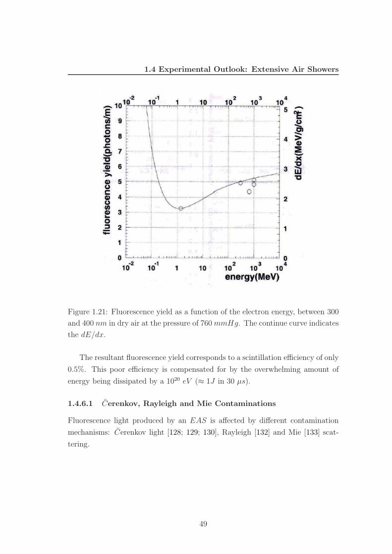
1.4 Experimental Outlook: Extensive Air Showers
Figure 1.21: Fluorescence yield as a function of the electron energy, between 300
and 400 nm in dry air at the pressure of 760 mmHg. The continue curve indicates
the dE/dx.
The resultant fluorescence yield corresponds to a scintillation efficiency of only
0.5%. This poor efficiency is compensated for by the overwhelming amount of
energy being dissipated by a 1020 eV (≈ 1J in 30 µs).
1.4.6.1 Cerenkov, Rayleigh and Mie Contaminations
Fluorescence light produced by an EAS is affected by different contamination
mechanisms: Cerenkov light [128; 129; 130], Rayleigh [132] and Mie [133] scat-
tering.
49
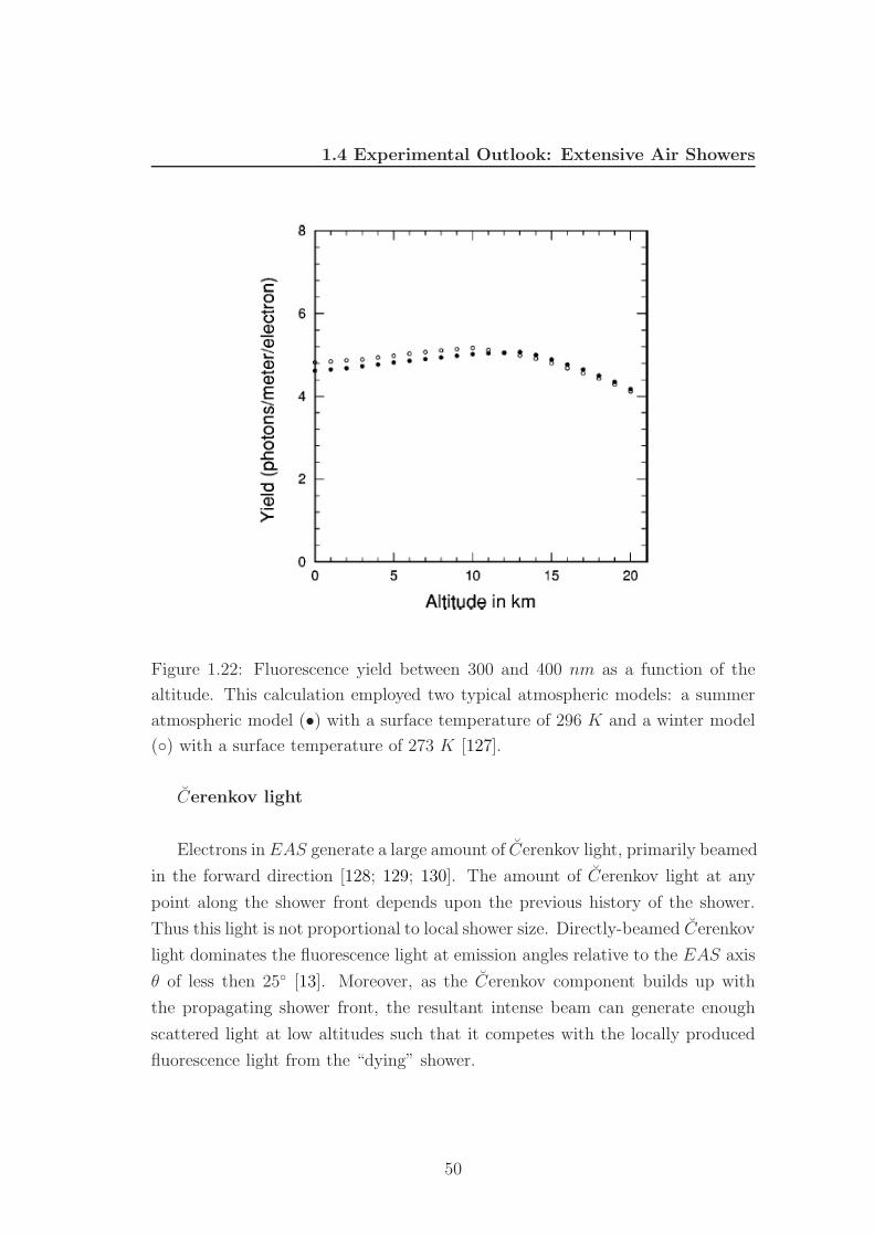
1.4 Experimental Outlook: Extensive Air Showers
Figure 1.22: Fluorescence yield between 300 and 400 nm as a function of the
altitude. This calculation employed two typical atmospheric models: a summer
atmospheric model (•) with a surface temperature of 296 K and a winter model
() with a surface temperature of 273 K [127].
Cerenkov light
Electrons in EAS generate a large amount of Cerenkov light, primarily beamed
in the forward direction [128; 129; 130]. The amount of Cerenkov light at any
point along the shower front depends upon the previous history of the shower.
Thus this light is not proportional to local shower size. Directly-beamed Cerenkov
light dominates the fluorescence light at emission angles relative to the EAS axis
θ of less then 25 [13]. Moreover, as the Cerenkov component builds up with
the propagating shower front, the resultant intense beam can generate enough
scattered light at low altitudes such that it competes with the locally produced
fluorescence light from the “dying” shower.
50
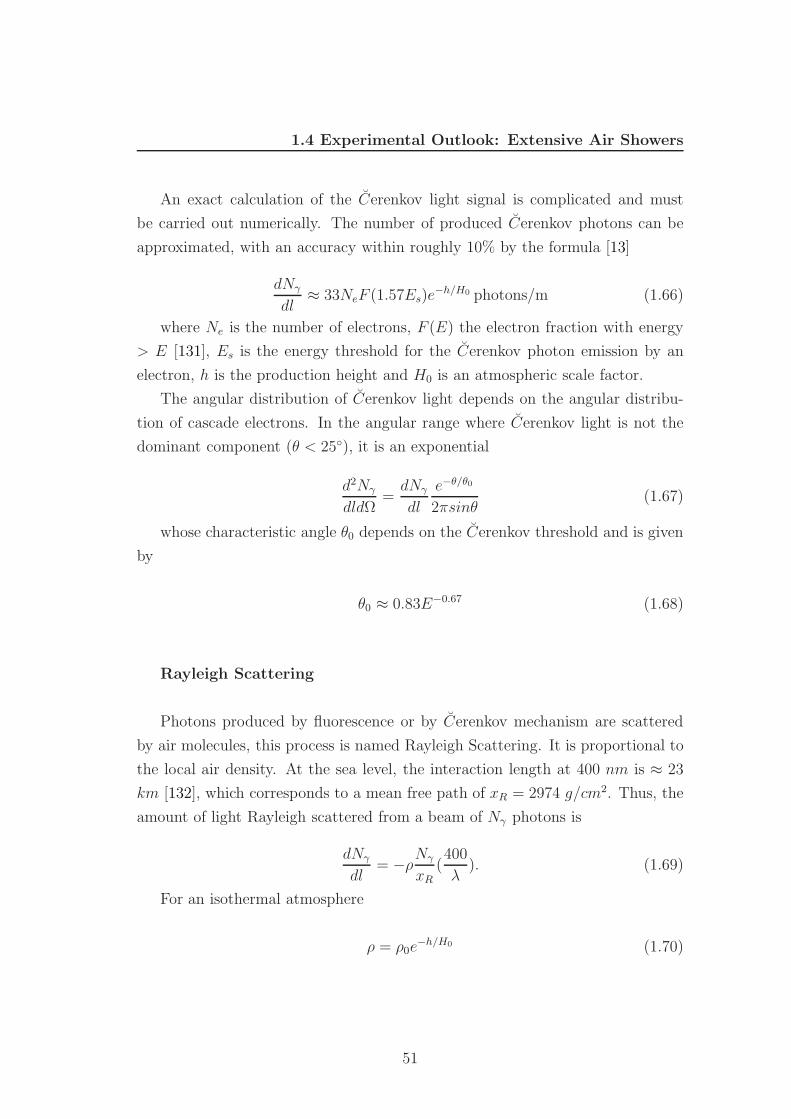
1.4 Experimental Outlook: Extensive Air Showers
An exact calculation of the Cerenkov light signal is complicated and must
be carried out numerically. The number of produced Cerenkov photons can be
approximated, with an accuracy within roughly 10% by the formula [13]
dNγ
dl≈ 33NeF (1.57Es)e
−h/H0 photons/m (1.66)
where Ne is the number of electrons, F (E) the electron fraction with energy
> E [131], Es is the energy threshold for the Cerenkov photon emission by an
electron, h is the production height and H0 is an atmospheric scale factor.
The angular distribution of Cerenkov light depends on the angular distribu-
tion of cascade electrons. In the angular range where Cerenkov light is not the
dominant component (θ < 25), it is an exponential
d2Nγ
dldΩ=
dNγ
dl
e−θ/θ0
2πsinθ(1.67)
whose characteristic angle θ0 depends on the Cerenkov threshold and is given
by
θ0 ≈ 0.83E−0.67 (1.68)
Rayleigh Scattering
Photons produced by fluorescence or by Cerenkov mechanism are scattered
by air molecules, this process is named Rayleigh Scattering. It is proportional to
the local air density. At the sea level, the interaction length at 400 nm is ≈ 23
km [132], which corresponds to a mean free path of xR = 2974 g/cm2. Thus, the
amount of light Rayleigh scattered from a beam of Nγ photons is
dNγ
dl= −ρ
Nγ
xR(400
λ). (1.69)
For an isothermal atmosphere
ρ = ρ0e−h/H0 (1.70)
51
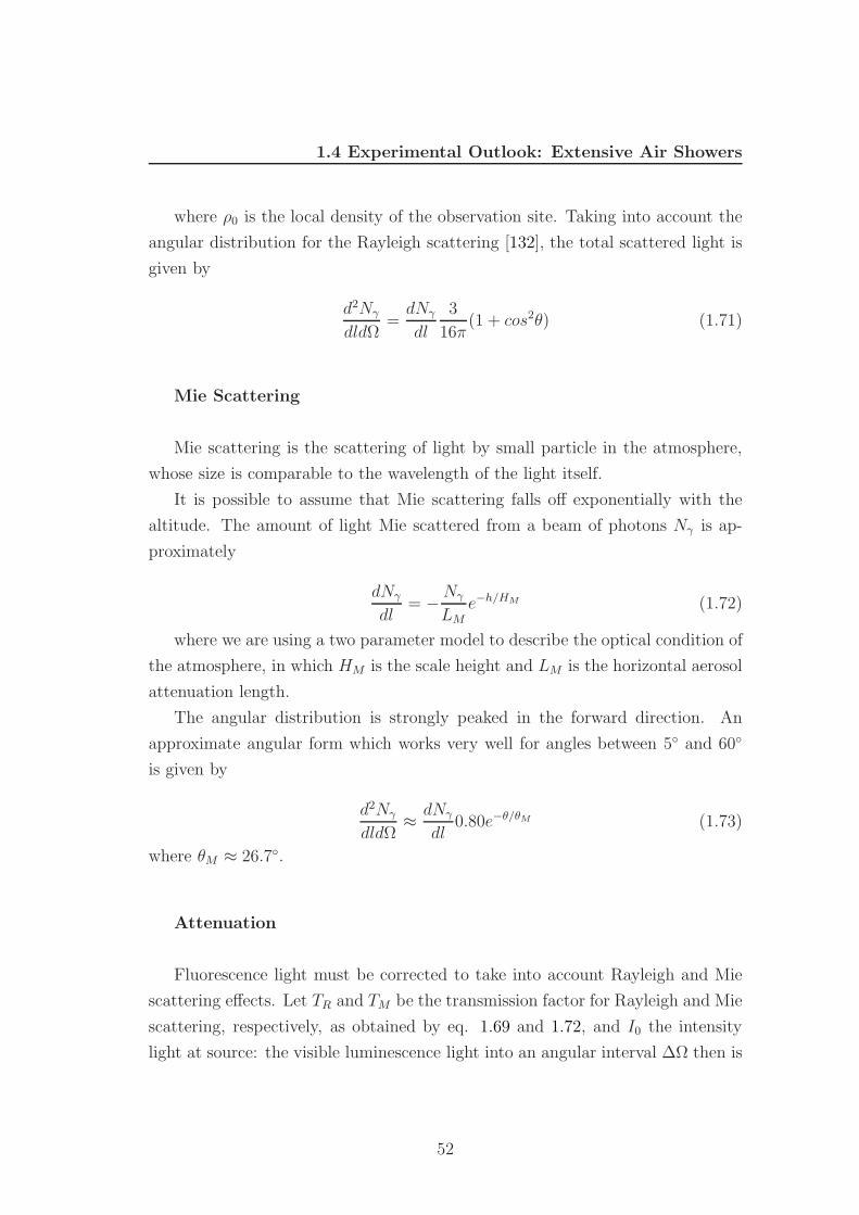
1.4 Experimental Outlook: Extensive Air Showers
where ρ0 is the local density of the observation site. Taking into account the
angular distribution for the Rayleigh scattering [132], the total scattered light is
given by
d2Nγ
dldΩ=
dNγ
dl
3
16π(1 + cos2θ) (1.71)
Mie Scattering
Mie scattering is the scattering of light by small particle in the atmosphere,
whose size is comparable to the wavelength of the light itself.
It is possible to assume that Mie scattering falls off exponentially with the
altitude. The amount of light Mie scattered from a beam of photons Nγ is ap-
proximately
dNγ
dl= − Nγ
LMe−h/HM (1.72)
where we are using a two parameter model to describe the optical condition of
the atmosphere, in which HM is the scale height and LM is the horizontal aerosol
attenuation length.
The angular distribution is strongly peaked in the forward direction. An
approximate angular form which works very well for angles between 5 and 60
is given by
d2Nγ
dldΩ≈ dNγ
dl0.80e−θ/θM (1.73)
where θM ≈ 26.7.
Attenuation
Fluorescence light must be corrected to take into account Rayleigh and Mie
scattering effects. Let TR and TM be the transmission factor for Rayleigh and Mie
scattering, respectively, as obtained by eq. 1.69 and 1.72, and I0 the intensity
light at source: the visible luminescence light into an angular interval ∆Ω then is
52
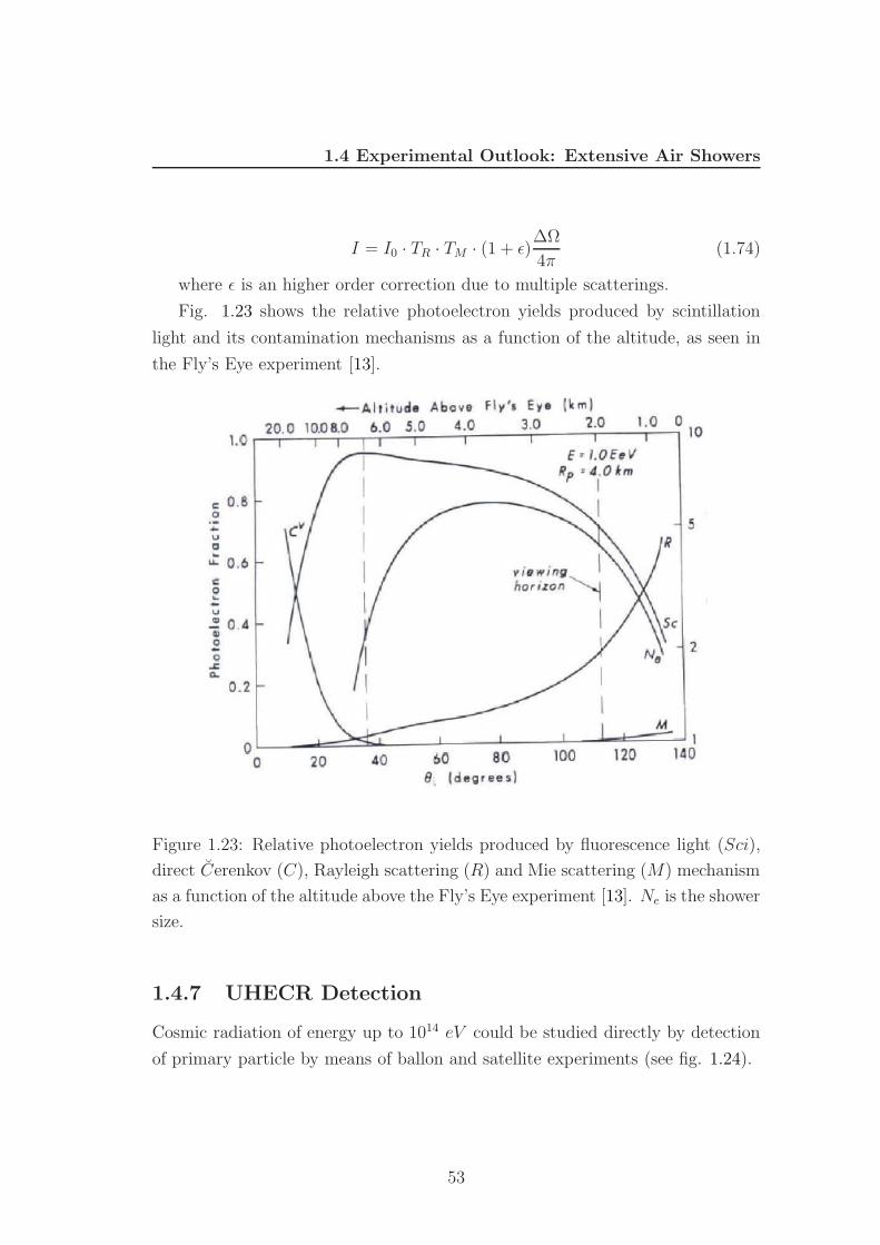
1.4 Experimental Outlook: Extensive Air Showers
I = I0 · TR · TM · (1 + ε)∆Ω
4π(1.74)
where ε is an higher order correction due to multiple scatterings.
Fig. 1.23 shows the relative photoelectron yields produced by scintillation
light and its contamination mechanisms as a function of the altitude, as seen in
the Fly’s Eye experiment [13].
Figure 1.23: Relative photoelectron yields produced by fluorescence light (Sci),
direct Cerenkov (C), Rayleigh scattering (R) and Mie scattering (M) mechanism
as a function of the altitude above the Fly’s Eye experiment [13]. Ne is the shower
size.
1.4.7 UHECR Detection
Cosmic radiation of energy up to 1014 eV could be studied directly by detection
of primary particle by means of ballon and satellite experiments (see fig. 1.24).
53
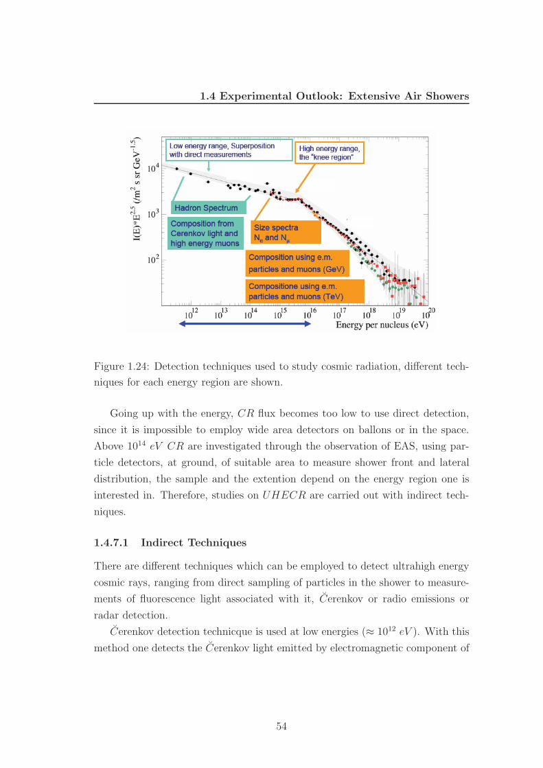
1.4 Experimental Outlook: Extensive Air Showers
Figure 1.24: Detection techniques used to study cosmic radiation, different tech-
niques for each energy region are shown.
Going up with the energy, CR flux becomes too low to use direct detection,
since it is impossible to employ wide area detectors on ballons or in the space.
Above 1014 eV CR are investigated through the observation of EAS, using par-
ticle detectors, at ground, of suitable area to measure shower front and lateral
distribution, the sample and the extention depend on the energy region one is
interested in. Therefore, studies on UHECR are carried out with indirect tech-
niques.
1.4.7.1 Indirect Techniques
There are different techniques which can be employed to detect ultrahigh energy
cosmic rays, ranging from direct sampling of particles in the shower to measure-
ments of fluorescence light associated with it, Cerenkov or radio emissions or
radar detection.
Cerenkov detection technicque is used at low energies (≈ 1012 eV ). With this
method one detects the Cerenkov light emitted by electromagnetic component of
54
1.4 Experimental Outlook: Extensive Air Showers
showers. Of course, this kind of experiments could only work during dark nights
with cloudless sky.
At higher energies, for UHECR, the two mostly employed detection te-
chiniques are the Surface array and the air fluorescence techniques.
Radio emission technique is now tested for the first time with the KASKADE−Grande [138] experiment and will be tested even in the Auger Observatory. More
recently, it has been proposed a technique in which one detect radar echos from
the column of ionized air produced by the shower.
Surface Arrays
Direct detection of shower particles with surface arrays is the most commonly
used method and involves an array of sensors spread over a wide area to sample
particle densities as the shower reaches at the ground. Sensors could be particle
detectors like plastic scintillators (used by AGASA experiment) or Cerenkov
radiators (employed by Haverah Park and AUGER Observatory). The two main
parameters of such detectors are the array surface and the detector spacing. The
total surface is chosen to match the expected incident flux, while the spacing
determines the threshold energy for a vertical shower. For Haverah park, a spacing
of 500 m was used, corresponding to a threshold of ≈ 1016 eV , for the Auger
Observatory a value of 1.5 km fix the trigger efficency to 1 at 1019 eV .
Such detectors measure the energy deposited by particles produced by a
shower, as a function of the time. Then, from energy density measured at the
ground and the relative timing of hits in the different detectors, one can estimate
the energy and the direction of primary CR.
Air Fluorescence Detection
Above 1017 eV , the fluorescence light emission can be used. Since this mecha-
nism has a scintillation efficiency of 0.5%, only at these energies the light emitted
becomes really distinguishable from a background light coming from the stars
and the moon.
55
1.4 Experimental Outlook: Extensive Air Showers
The technique has been employed for the first time by Greisen [134] and his
group in 1965 but unsuccessfully. The first successful attempt to detect EAS with
fluorescence light observation was done by Utah University group [135]. They de-
tected fluorescence light in coincidence with Volcano Ranch surface array. The
first complete experiment was the Fly’s Eye experiment that started to take data
in 1982. Its name derived from its structure: 67 mirrors with 880 photomulti-
pliers, displaced over a semi-spherical surface. It has now been replaced by its
updated version, the High Resolution Fly’s Eye (HiRes).
From signal timing and intensity measured by such a detector it is possible to
reconstruct the axis and the longitudinal profile of a shower and then the energy
and the shower maximum. Further details will be given in chapter 3.
1.4.8 Fingerprints of primary species in EAS
The measurement of primary particle mass composition is crucial for testing any
theory of cosmic ray origin. However, this is the most difficult task facing an air
shower physicist. So far, no method has been applied for which the conclusion
is not dependent on the shower model used to describe the data. Furthermore,
a mass composition analysis should take into account of the shower-to-shower
fluctuations in measured shower observables.
Up to now, statistical analysis of shower observables known to correlate with
the primary composition have been developed.
1.4.8.1 Muon Component
It is easy to understand that one of the possibility of distinguish between different
particle species is offered by the muon content of showers. Using the superposition
principle to describe an hadronic cascade, it is clear that an iron nucleus should,
on average, produce more muon at ground level than a proton of the same energy,
because the mean energy of created pions is lower in a Fe−shower with respect
to a p−shower. There are different problems related to the measurement of
the muon content of showers as the cost, because large area muon detectors
are needed. Further, the muon content is very dependent on the multiplicity of
56

1.4 Experimental Outlook: Extensive Air Showers
charged particles. As an example, it is possible to consider the model used by
Gaisser [85]
Nµ(> 1GeV ) = 2.8A(E/Aεπ)0.86 (1.75)
where A is the mass of the primary particle of energy E and επ is the energy
associated with the competition between decay and interaction for pions (∼ 50
GeV ). In this model an iron should produce 76% more muons than a proton.
1.4.8.2 Elongation Rate
Linsley [136] pointed out that the variation of the depth of the shower maximum
with the energy (dlogXmax/dlogE) could be a useful indicator of the energy de-
pendence of the primary mass. In fact, changes in the mean mass composition
of the CR flux as a function of the energy should produce a change in the mean
value of the observable Xmax. This change is known as the elongation rate theo-
rem. For pure electromagnetic showers, Xmax(E) ≈ X0ln(E/ε0) (where ε0 is the
critical energy) and then the rate is dlogXmax/dlogE ≈ X0. For protons, using
the Heitler model, if 〈n(E)〉 is the mean number of secondary particles produced
by the first interaction and λN is its mean free path in the atmosphere, it follows
that
Xmax(E) = λN + X0ln[E/〈n(E)〉]. (1.76)
Assuming that 〈n(E)〉 ≈ n0E∆, the elongation rate can be expressed by the form
given by Linsley and Watson [137]
De = δXmax/δlnE = X0
[1 − δln〈n(E)〉
δlnE+
λN
X0
δln(λN )
δlnE
]= X0(1 − B) (1.77)
Using the superposition model and assuming that
B ≡ ∆ − λN
X0
δln(λN )
δlnE(1.78)
is not changing with the energy, one obtains for a mixed composition
De = X0(1 − B)
[1 − ð〈lnA〉
ð〈lnE〉]
(1.79)
Thus, the elongation rate provides a measurement of the change of the mean
logarithmic mass with energy.
57
1.4 Experimental Outlook: Extensive Air Showers
1.4.8.3 Temporal Distribution Of Shower Particles
The arrival time of the particles in the shower front is spread out because of
geometrical effects, velocity differences and delay produced by multiple scattering
and geomagnetic deflections (see section 1.4.4). As already said, muons are the
first particles to reach the ground. So for an iron nucleus, a signal shorter in
time with respect to a proton shower is produced. Thus a shower front structure
study could help to solve the mass composition puzzle. However, for techinal
limitations of past experiments, the Auger Observatory will be the first in which
will be possible to study it.
1.4.8.4 Lateral Distribution
The fall off of particles with the distance from the shower axis, the lateral density
distribution (see sec. 1.4.3) is another parameter that can be used to extract
the mass composition. Showers with steeper lateral distribution functions than
average will arise from showers that develop later in the atmosphere, like a proton,
and viceversa.
58
Chapter 2
The Pierre Auger Observatory
2.1 Introduction
The Pierre Auger Observatory (PAO) project is the biggest experiment on cosmic
rays even conceived. It was optimized to answer to all the open questions on
UHECR:
1. the spectrum in the GZK−region;
2. observation of point-like sources of cosmic rays (anisotropy on small scale);
3. estimation of intergalactic magnetic field;
4. observation of large scale anisotropy;
5. mass composition in the GZK−region;
Born in 1992 by two physicists, Jim Cronin and Alan Watson, the project idea
derives its name by the french physicist that discovered the extended air shower
existence.
The experiment involves several universities and research institutes from 18
countries, a collaboration with more than 300 physicists.
Its main characteristics are:
1. Full Sky coverage. The project consists of a two-sites observatory, one for
each terrestrial hemisphere, in order to provide a full sky coverage, crucial
59
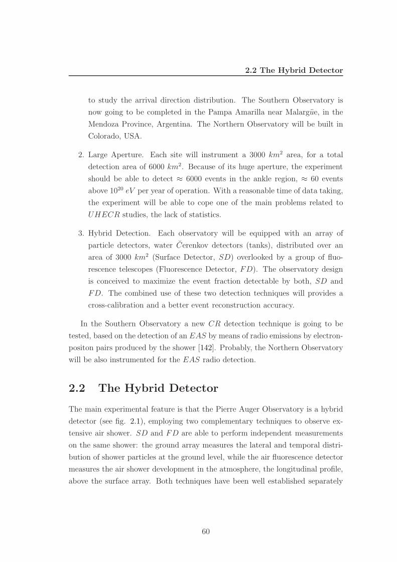
2.2 The Hybrid Detector
to study the arrival direction distribution. The Southern Observatory is
now going to be completed in the Pampa Amarilla near Malargue, in the
Mendoza Province, Argentina. The Northern Observatory will be built in
Colorado, USA.
2. Large Aperture. Each site will instrument a 3000 km2 area, for a total
detection area of 6000 km2. Because of its huge aperture, the experiment
should be able to detect ≈ 6000 events in the ankle region, ≈ 60 events
above 1020 eV per year of operation. With a reasonable time of data taking,
the experiment will be able to cope one of the main problems related to
UHECR studies, the lack of statistics.
3. Hybrid Detection. Each observatory will be equipped with an array of
particle detectors, water Cerenkov detectors (tanks), distributed over an
area of 3000 km2 (Surface Detector, SD) overlooked by a group of fluo-
rescence telescopes (Fluorescence Detector, FD). The observatory design
is conceived to maximize the event fraction detectable by both, SD and
FD. The combined use of these two detection techniques will provides a
cross-calibration and a better event reconstruction accuracy.
In the Southern Observatory a new CR detection technique is going to be
tested, based on the detection of an EAS by means of radio emissions by electron-
positon pairs produced by the shower [142]. Probably, the Northern Observatory
will be also instrumented for the EAS radio detection.
2.2 The Hybrid Detector
The main experimental feature is that the Pierre Auger Observatory is a hybrid
detector (see fig. 2.1), employing two complementary techniques to observe ex-
tensive air shower. SD and FD are able to perform independent measurements
on the same shower: the ground array measures the lateral and temporal distri-
bution of shower particles at the ground level, while the air fluorescence detector
measures the air shower development in the atmosphere, the longitudinal profile,
above the surface array. Both techniques have been well established separately
60
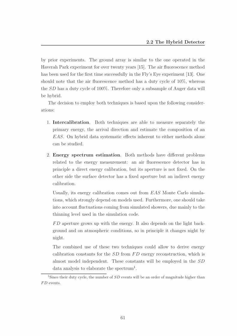
2.2 The Hybrid Detector
by prior experiments. The ground array is similar to the one operated in the
Haverah Park experiment for over twenty years [15]. The air fluorescence method
has been used for the first time successfully in the Fly’s Eye experiment [13]. One
should note that the air fluorescence method has a duty cycle of 10%, whereas
the SD has a duty cycle of 100%. Therefore only a subsample of Auger data will
be hybrid.
The decision to employ both techniques is based upon the following consider-
ations:
1. Intercalibration. Both techniques are able to measure separately the
primary energy, the arrival direction and estimate the composition of an
EAS. On hybrid data systematic effects inherent to either methods alone
can be studied.
2. Energy spectrum estimation. Both methods have different problems
related to the energy measurement: an air fluorescence detector has in
principle a direct energy calibration, but its aperture is not fixed. On the
other side the surface detector has a fixed aperture but an indirect energy
calibration.
Usually, its energy calibration comes out from EAS Monte Carlo simula-
tions, which strongly depend on models used. Furthermore, one should take
into account fluctuations coming from simulated showers, due mainly to the
thinning level used in the simulation code.
FD aperture grows up with the energy. It also depends on the light back-
ground and on atmospheric conditions, so in principle it changes night by
night.
The combined use of these two techniques could allow to derive energy
calibration constants for the SD from FD energy reconstruction, which is
almost model independent. These constants will be employed in the SD
data analysis to elaborate the spectrum1.
1Since their duty cycle, the number of SD events will be an order of magnitude higher thanFD events.
61

2.2 The Hybrid Detector
Figure 2.1: Hybrid detection scheme: shower particles are sampled at ground
level by Cerenkov detectors while the fluorescence detector records fluorescence
light produced by shower particles through excitation of nitrogen molecules as
the shower develops in the atmosphere.
62
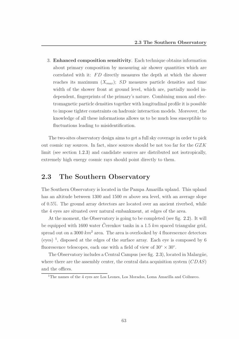
2.3 The Southern Observatory
3. Enhanced composition sensitivity. Each technique obtains information
about primary composition by measuring air shower quantities which are
correlated with it: FD directly measures the depth at which the shower
reaches its maximum (Xmax); SD measures particle densities and time
width of the shower front at ground level, which are, partially model in-
dependent, fingerprints of the primary’s nature. Combining muon and elec-
tromagnetic particle densities together with longitudinal profile it is possible
to impose tighter constraints on hadronic interaction models. Moreover, the
knowledge of all these informations allows us to be much less susceptible to
fluctuations leading to misidentification.
The two-sites observatory design aims to get a full sky coverage in order to pick
out cosmic ray sources. In fact, since sources should be not too far for the GZK
limit (see section 1.2.3) and candidate sources are distributed not isotropically,
extremely high energy cosmic rays should point directly to them.
2.3 The Southern Observatory
The Southern Observatory is located in the Pampa Amarilla upland. This upland
has an altitude between 1300 and 1500 m above sea level, with an average slope
of 0.5%. The ground array detectors are located over an ancient riverbed, while
the 4 eyes are situated over natural embankment, at edges of the area.
At the moment, the Observatory is going to be completed (see fig. 2.2). It will
be equipped with 1600 water Cerenkov tanks in a 1.5 km spaced triangular grid,
spread out on a 3000 km2 area. The area is overlooked by 4 fluorescence detectors
(eyes) 1, disposed at the edges of the surface array. Each eye is composed by 6
fluorescence telescopes, each one with a field of view of 30 × 30.
The Observatory includes a Central Campus (see fig. 2.3), located in Malargue,
where there are the assembly center, the central data acquisition system (CDAS)
and the offices.
1The names of the 4 eyes are Los Leones, Los Morados, Loma Amarilla and Coihueco.
63
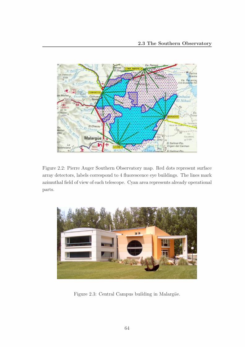
2.3 The Southern Observatory
Figure 2.2: Pierre Auger Southern Observatory map. Red dots represent surface
array detectors, labels correspond to 4 fluorescence eye buildings. The lines mark
azimuthal field of view of each telescope. Cyan area represents already operational
parts.
Figure 2.3: Central Campus building in Malargue.
64
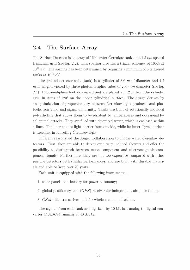
2.4 The Surface Array
2.4 The Surface Array
The Surface Detector is an array of 1600 water Cerenkov tanks in a 1.5 km spaced
triangular grid (see fig. 2.2). This spacing provides a trigger efficency of 100% at
1019 eV . The spacing has been determined by requiring a minimum of 5 triggered
tanks at 1019 eV .
The ground detector unit (tank) is a cylinder of 3.6 m of diameter and 1.2
m in height, viewed by three photomultiplier tubes of 200 mm diameter (see fig.
2.4). Photomulipliers look downward and are placed at 1.2 m from the cylinder
axis, in steps of 120 on the upper cylindrical surface. The design derives by
an optimization of proportionality between Cerenkov light produced and pho-
toelectron yield and signal uniformity. Tanks are built of rotationally moulded
polyethylene that allows them to be resistent to temperatures and occasional lo-
cal animal attacks. They are filled with deionized water, which is enclosed within
a liner. The liner acts as light barrier from outside, while its inner Tyvek surface
is excellent in reflecting Cerenkov light.
Different reasons led the Auger Collaboration to choose water Cerenkov de-
tectors. First, they are able to detect even very inclined showers and offer the
possibility to distinguish between muon component and electromagnetic com-
ponent signals. Furthermore, they are not too expensive compared with other
particle detectors with similar performances, and are built with durable materi-
als and able to keep over 20 years.
Each unit is equipped with the following instruments::
1. solar panels and battery for power autonomy;
2. global position system (GPS) receiver for independent absolute timing;
3. GSM−like transceiver unit for wireless communications.
The signals from each tank are digitized by 10 bit fast analog to digital con-
verter (FADCs) running at 40 MHz.
65
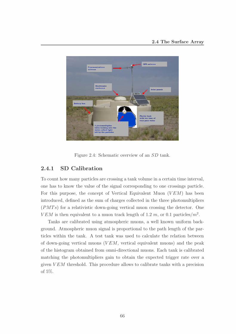
2.4 The Surface Array
Figure 2.4: Schematic overview of an SD tank.
2.4.1 SD Calibration
To count how many particles are crossing a tank volume in a certain time interval,
one has to know the value of the signal corresponding to one crossings particle.
For this purpose, the concept of Vertical Equivalent Muon (V EM) has been
introduced, defined as the sum of charges collected in the three photomultipliers
(PMTs) for a relativistic down-going vertical muon crossing the detector. One
V EM is then equivalent to a muon track length of 1.2 m, or 0.1 particles/m2.
Tanks are calibrated using atmospheric muons, a well known uniform back-
ground. Atmospheric muon signal is proportional to the path length of the par-
ticles within the tank. A test tank was used to calculate the relation between
of down-going vertical muons (V EM , vertical equivalent muons) and the peak
of the histogram obtained from omni-directional muons. Each tank is calibrated
matching the photomultipliers gain to obtain the expected trigger rate over a
given V EM threshold. This procedure allows to calibrate tanks with a precision
of 5%.
66
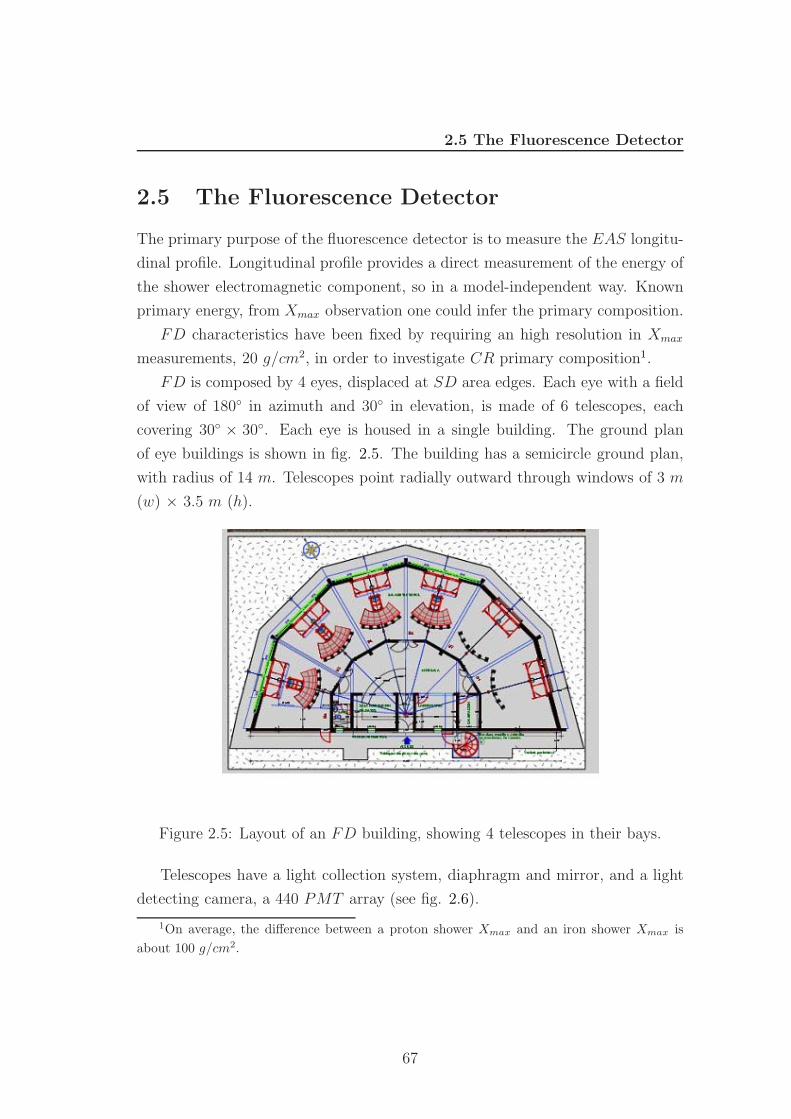
2.5 The Fluorescence Detector
2.5 The Fluorescence Detector
The primary purpose of the fluorescence detector is to measure the EAS longitu-
dinal profile. Longitudinal profile provides a direct measurement of the energy of
the shower electromagnetic component, so in a model-independent way. Known
primary energy, from Xmax observation one could infer the primary composition.
FD characteristics have been fixed by requiring an high resolution in Xmax
measurements, 20 g/cm2, in order to investigate CR primary composition1.
FD is composed by 4 eyes, displaced at SD area edges. Each eye with a field
of view of 180 in azimuth and 30 in elevation, is made of 6 telescopes, each
covering 30 × 30. Each eye is housed in a single building. The ground plan
of eye buildings is shown in fig. 2.5. The building has a semicircle ground plan,
with radius of 14 m. Telescopes point radially outward through windows of 3 m
(w) × 3.5 m (h).
Figure 2.5: Layout of an FD building, showing 4 telescopes in their bays.
Telescopes have a light collection system, diaphragm and mirror, and a light
detecting camera, a 440 PMT array (see fig. 2.6).
1On average, the difference between a proton shower Xmax and an iron shower Xmax isabout 100 g/cm2.
67
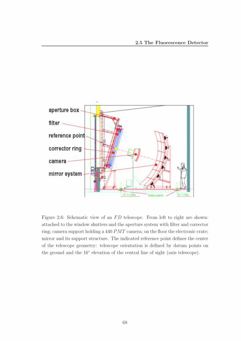
2.5 The Fluorescence Detector
Figure 2.6: Schematic view of an FD telescope. From left to right are shown:
attached to the window shutters and the aperture system with filter and corrector
ring; camera support holding a 440 PMT camera; on the floor the electronic crate;
mirror and its support structure. The indicated reference point defines the center
of the telescope geometry: telescope orientation is defined by datum points on
the ground and the 16 elevation of the central line of sight (axis telescope).
68
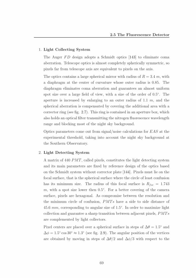
2.5 The Fluorescence Detector
1. Light Collecting System
The Auger FD design adopts a Schmidt optics [143] to eliminate coma
aberration. Telescope optics is almost completely spherically symmetric, so
pixels far from telescope axis are equivalent to pixels on the axis.
The optics contains a large spherical mirror with radius of R = 3.4 m, with
a diaphragm at the center of curvature whose outer radius is 0.85. The
diaphragm eliminates coma aberration and guarantees an almost uniform
spot size over a large field of view, with a size of the order of 0.5. The
aperture is increased by enlarging to an outer radius of 1.1 m, and the
spherical aberration is compensated by covering the additional area with a
corrector ring (see fig. 2.7). This ring is contained in an aperture box, which
also holds an optical filter transmitting the nitrogen fluorescence wavelength
range and blocking most of the night sky background.
Optics parameters come out from signal/noise calculations for EAS at the
experimental threshold, taking into account the night sky background at
the Southern Observatory.
2. Light Detecting System
A matrix of 440 PMT , called pixels, constitutes the light detecting system
and its main parameters are fixed by reference design of the optics based
on the Schmidt system without corrector plate [144]. Pixels must lie on the
focal surface, that is the spherical surface where the circle of least confusion
has its minimum size. The radius of this focal surface is Rfoc = 1.743
m, with a spot size lower then 0.5. For a better covering of the camera
surface, pixels are hexagonal. As compromise between the resolution and
the minimum circle of confusion, PMTs have a side to side distance of
45.6 mm, corresponding to angular size of 1.5. In order to maximize light
collection and guarantee a sharp transition between adjacent pixels, PMTs
are complemented by light collectors.
Pixel centers are placed over a spherical surface in steps of ∆θ = 1.5 and
∆φ = 1.5 cos 30 ≈ 1.3 (see fig. 2.9). The angular position of the vertices
are obtained by moving in steps of ∆θ/2 and ∆φ/3 with respect to the
69
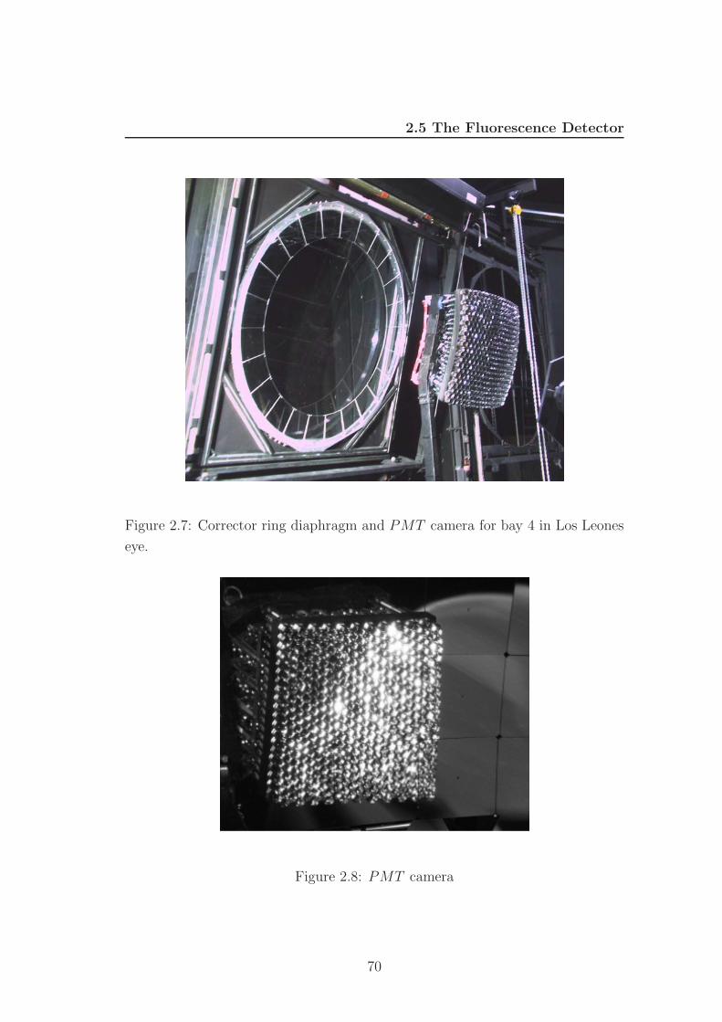
2.5 The Fluorescence Detector
Figure 2.7: Corrector ring diaphragm and PMT camera for bay 4 in Los Leones
eye.
Figure 2.8: PMT camera
70
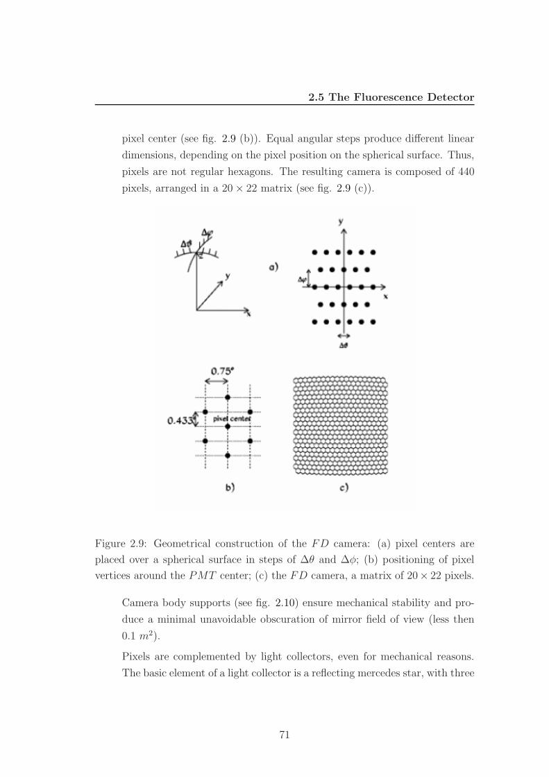
2.5 The Fluorescence Detector
pixel center (see fig. 2.9 (b)). Equal angular steps produce different linear
dimensions, depending on the pixel position on the spherical surface. Thus,
pixels are not regular hexagons. The resulting camera is composed of 440
pixels, arranged in a 20 × 22 matrix (see fig. 2.9 (c)).
Figure 2.9: Geometrical construction of the FD camera: (a) pixel centers are
placed over a spherical surface in steps of ∆θ and ∆φ; (b) positioning of pixel
vertices around the PMT center; (c) the FD camera, a matrix of 20× 22 pixels.
Camera body supports (see fig. 2.10) ensure mechanical stability and pro-
duce a minimal unavoidable obscuration of mirror field of view (less then
0.1 m2).
Pixels are complemented by light collectors, even for mechanical reasons.
The basic element of a light collector is a reflecting mercedes star, with three
71
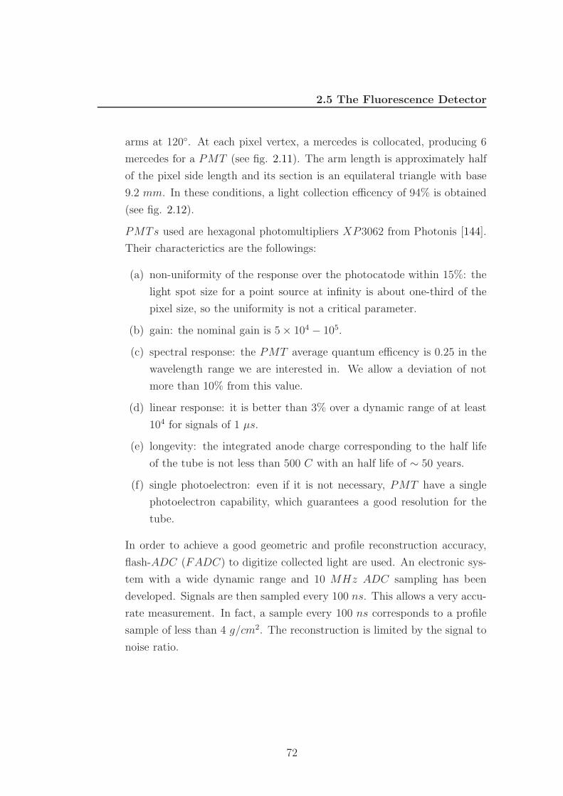
2.5 The Fluorescence Detector
arms at 120. At each pixel vertex, a mercedes is collocated, producing 6
mercedes for a PMT (see fig. 2.11). The arm length is approximately half
of the pixel side length and its section is an equilateral triangle with base
9.2 mm. In these conditions, a light collection efficency of 94% is obtained
(see fig. 2.12).
PMTs used are hexagonal photomultipliers XP3062 from Photonis [144].
Their characterictics are the followings:
(a) non-uniformity of the response over the photocatode within 15%: the
light spot size for a point source at infinity is about one-third of the
pixel size, so the uniformity is not a critical parameter.
(b) gain: the nominal gain is 5 × 10⁴ − 105.
(c) spectral response: the PMT average quantum efficency is 0.25 in the
wavelength range we are interested in. We allow a deviation of not
more than 10% from this value.
(d) linear response: it is better than 3% over a dynamic range of at least
104 for signals of 1 µs.
(e) longevity: the integrated anode charge corresponding to the half life
of the tube is not less than 500 C with an half life of ∼ 50 years.
(f) single photoelectron: even if it is not necessary, PMT have a single
photoelectron capability, which guarantees a good resolution for the
tube.
In order to achieve a good geometric and profile reconstruction accuracy,
flash-ADC (FADC) to digitize collected light are used. An electronic sys-
tem with a wide dynamic range and 10 MHz ADC sampling has been
developed. Signals are then sampled every 100 ns. This allows a very accu-
rate measurement. In fact, a sample every 100 ns corresponds to a profile
sample of less than 4 g/cm2. The reconstruction is limited by the signal to
noise ratio.
72
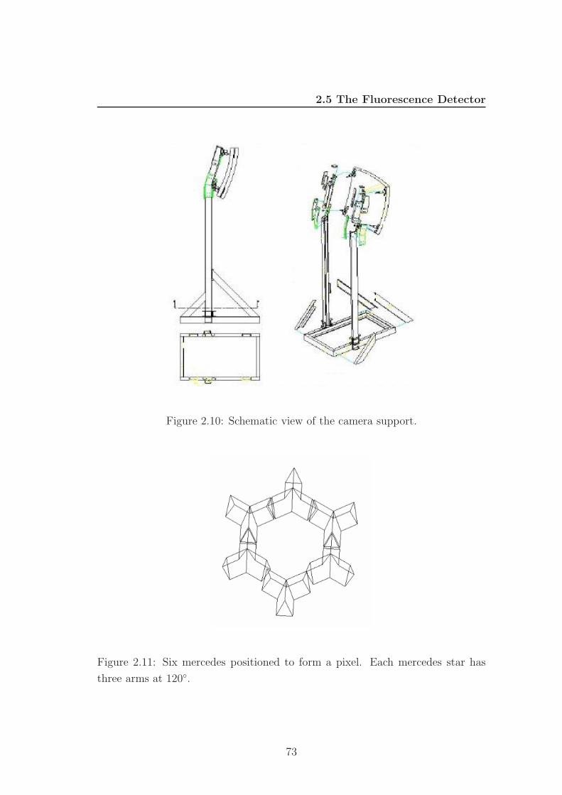
2.5 The Fluorescence Detector
Figure 2.10: Schematic view of the camera support.
Figure 2.11: Six mercedes positioned to form a pixel. Each mercedes star has
three arms at 120.
73
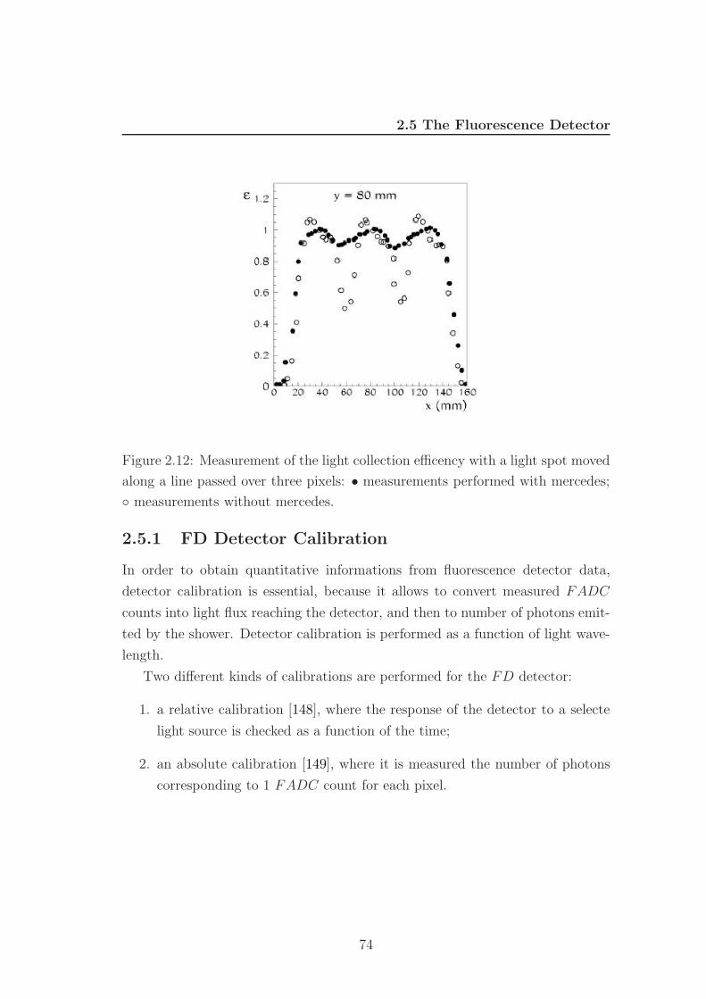
2.5 The Fluorescence Detector
Figure 2.12: Measurement of the light collection efficency with a light spot moved
along a line passed over three pixels: • measurements performed with mercedes;
measurements without mercedes.
2.5.1 FD Detector Calibration
In order to obtain quantitative informations from fluorescence detector data,
detector calibration is essential, because it allows to convert measured FADC
counts into light flux reaching the detector, and then to number of photons emit-
ted by the shower. Detector calibration is performed as a function of light wave-
length.
Two different kinds of calibrations are performed for the FD detector:
1. a relative calibration [148], where the response of the detector to a selecte
light source is checked as a function of the time;
2. an absolute calibration [149], where it is measured the number of photons
corresponding to 1 FADC count for each pixel.
74
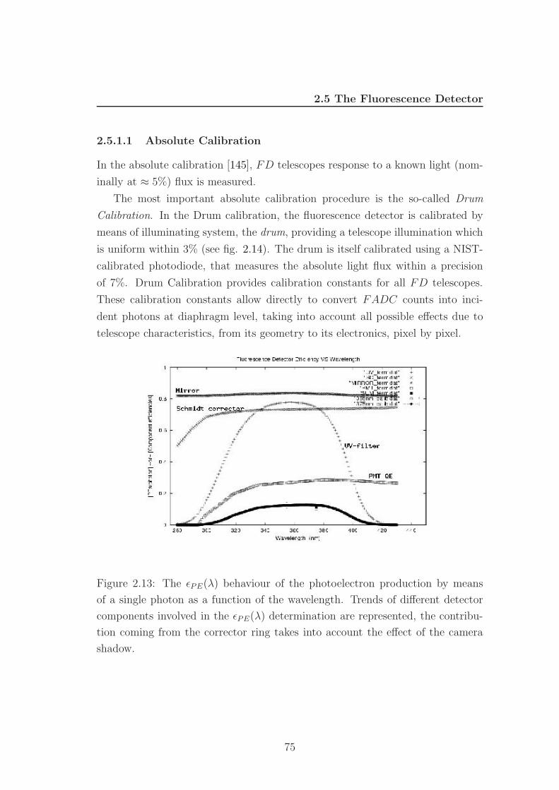
2.5 The Fluorescence Detector
2.5.1.1 Absolute Calibration
In the absolute calibration [145], FD telescopes response to a known light (nom-
inally at ≈ 5%) flux is measured.
The most important absolute calibration procedure is the so-called Drum
Calibration. In the Drum calibration, the fluorescence detector is calibrated by
means of illuminating system, the drum, providing a telescope illumination which
is uniform within 3% (see fig. 2.14). The drum is itself calibrated using a NIST-
calibrated photodiode, that measures the absolute light flux within a precision
of 7%. Drum Calibration provides calibration constants for all FD telescopes.
These calibration constants allow directly to convert FADC counts into inci-
dent photons at diaphragm level, taking into account all possible effects due to
telescope characteristics, from its geometry to its electronics, pixel by pixel.
Figure 2.13: The εPE(λ) behaviour of the photoelectron production by means
of a single photon as a function of the wavelength. Trends of different detector
components involved in the εPE(λ) determination are represented, the contribu-
tion coming from the corrector ring takes into account the effect of the camera
shadow.
75
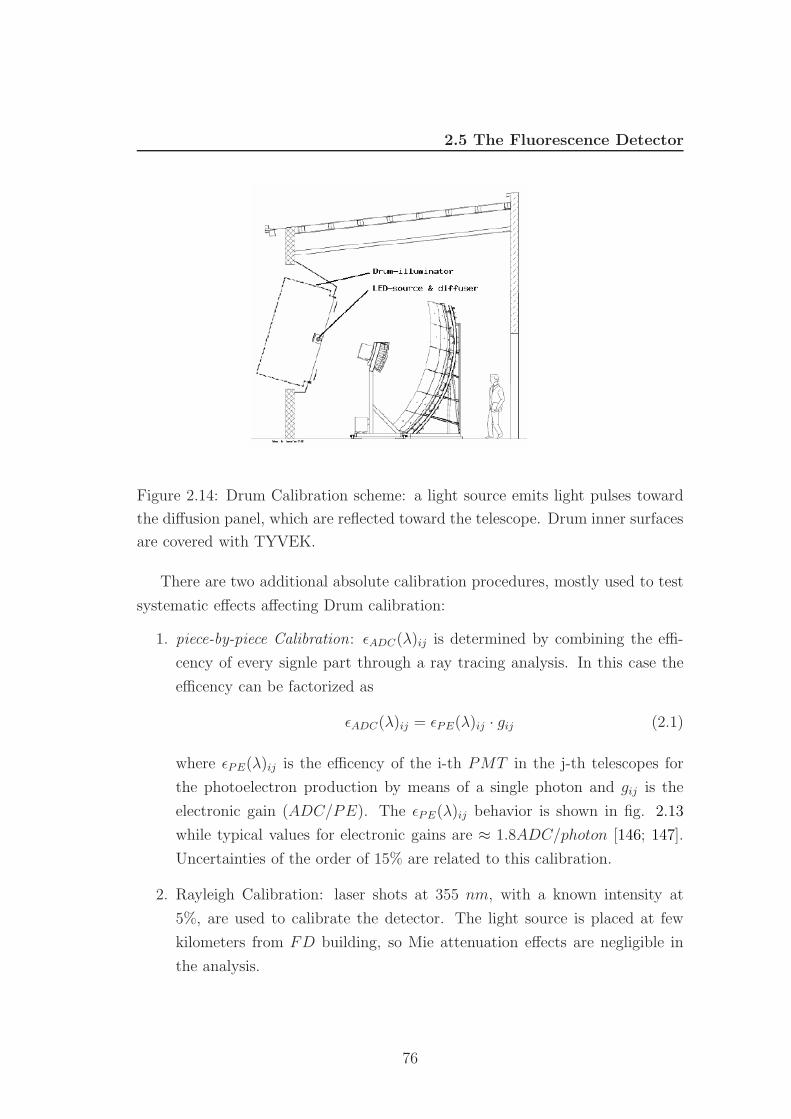
2.5 The Fluorescence Detector
Figure 2.14: Drum Calibration scheme: a light source emits light pulses toward
the diffusion panel, which are reflected toward the telescope. Drum inner surfaces
are covered with TYVEK.
There are two additional absolute calibration procedures, mostly used to test
systematic effects affecting Drum calibration:
1. piece-by-piece Calibration: εADC(λ)ij is determined by combining the effi-
cency of every signle part through a ray tracing analysis. In this case the
efficency can be factorized as
εADC(λ)ij = εPE(λ)ij · gij (2.1)
where εPE(λ)ij is the efficency of the i-th PMT in the j-th telescopes for
the photoelectron production by means of a single photon and gij is the
electronic gain (ADC/PE). The εPE(λ)ij behavior is shown in fig. 2.13
while typical values for electronic gains are ≈ 1.8ADC/photon [146; 147].
Uncertainties of the order of 15% are related to this calibration.
2. Rayleigh Calibration: laser shots at 355 nm, with a known intensity at
5%, are used to calibrate the detector. The light source is placed at few
kilometers from FD building, so Mie attenuation effects are negligible in
the analysis.
76
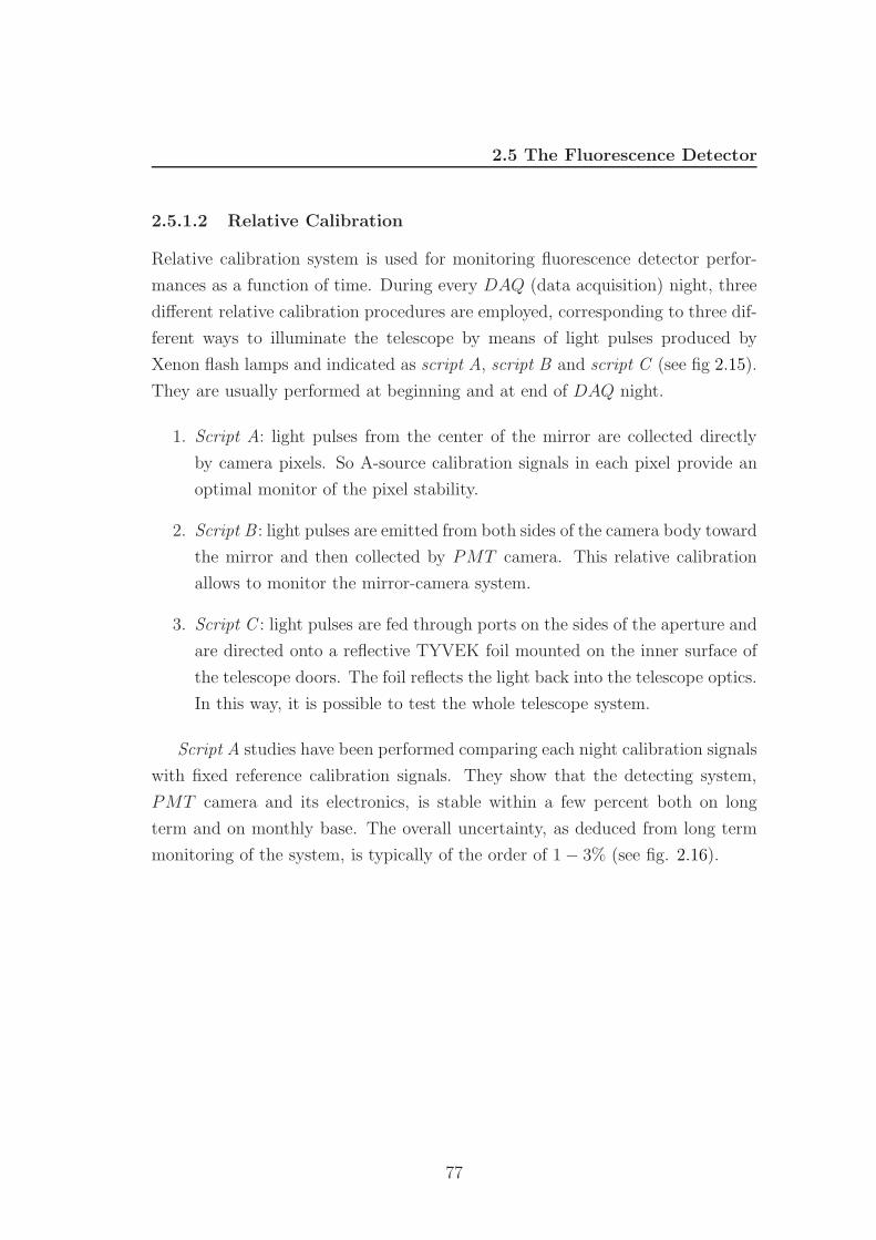
2.5 The Fluorescence Detector
2.5.1.2 Relative Calibration
Relative calibration system is used for monitoring fluorescence detector perfor-
mances as a function of time. During every DAQ (data acquisition) night, three
different relative calibration procedures are employed, corresponding to three dif-
ferent ways to illuminate the telescope by means of light pulses produced by
Xenon flash lamps and indicated as script A, script B and script C (see fig 2.15).
They are usually performed at beginning and at end of DAQ night.
1. Script A: light pulses from the center of the mirror are collected directly
by camera pixels. So A-source calibration signals in each pixel provide an
optimal monitor of the pixel stability.
2. Script B : light pulses are emitted from both sides of the camera body toward
the mirror and then collected by PMT camera. This relative calibration
allows to monitor the mirror-camera system.
3. Script C : light pulses are fed through ports on the sides of the aperture and
are directed onto a reflective TYVEK foil mounted on the inner surface of
the telescope doors. The foil reflects the light back into the telescope optics.
In this way, it is possible to test the whole telescope system.
Script A studies have been performed comparing each night calibration signals
with fixed reference calibration signals. They show that the detecting system,
PMT camera and its electronics, is stable within a few percent both on long
term and on monthly base. The overall uncertainty, as deduced from long term
monitoring of the system, is typically of the order of 1 − 3% (see fig. 2.16).
77
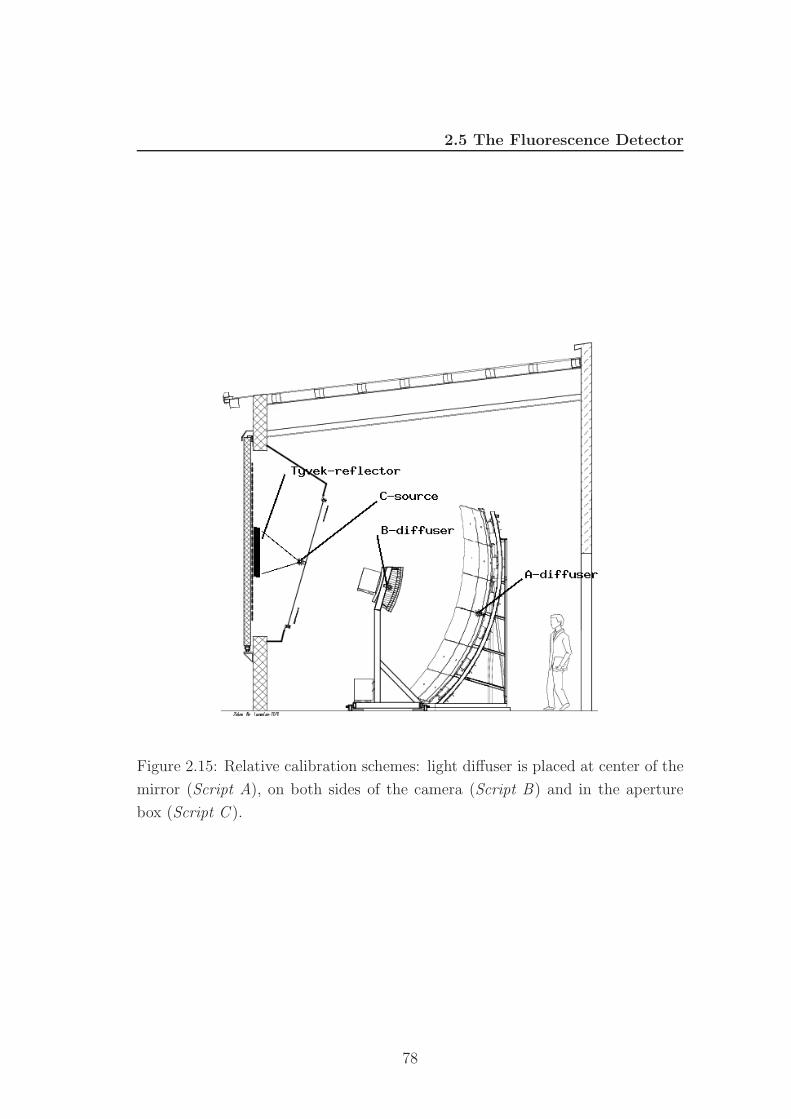
2.5 The Fluorescence Detector
Figure 2.15: Relative calibration schemes: light diffuser is placed at center of the
mirror (Script A), on both sides of the camera (Script B) and in the aperture
box (Script C ).
78
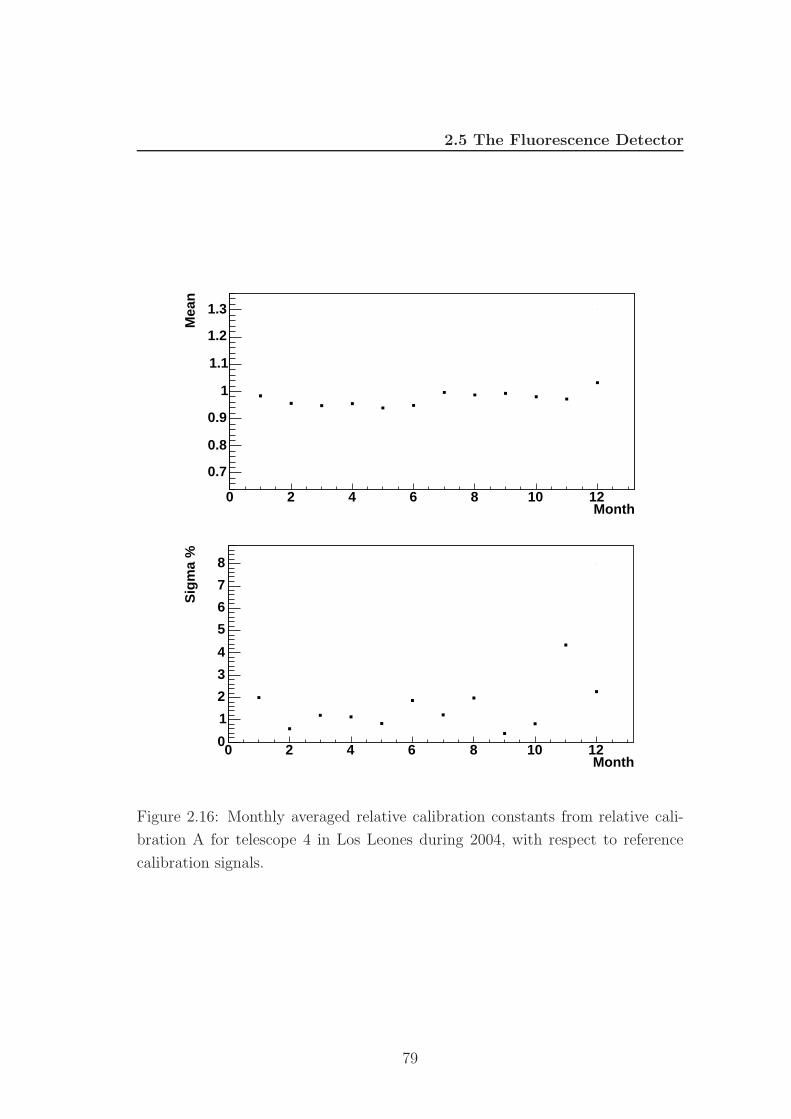
2.5 The Fluorescence Detector
Month0 2 4 6 8 10 12
Mea
n
0.7
0.8
0.9
1
1.1
1.2
1.3
Month0 2 4 6 8 10 12
Sig
ma
%
0
1
2
3
4
5
6
7
8
Figure 2.16: Monthly averaged relative calibration constants from relative cali-
bration A for telescope 4 in Los Leones during 2004, with respect to reference
calibration signals.
79
2.6 Atmospheric Monitoring
2.6 Atmospheric Monitoring
Experiments based on EAS detection use the atmosphere as a huge calorimeter,
whose properties vary in a predictable way with altitude and in a relatively unpre-
dictable way with time. As in the “usual” calorimeters, one has to get a complete
description of its properties. In fact, to get a precise estimation of the amount of
the fluorescence light emitted by the cosmic ray shower and to be able to convert
production height in atmospheric depth passed through by the shower, a detailed
knowledge of the atmospheric conditions is required. The largest uncertaities in
the fluorescence measurements come from uncertainties in the atmospheric trans-
mission1, air Cerenkov subtraction, light multiple scattering. To minimize the
atmospheric uncertainties, Southern and Northern Observatory will be located in
dry desert areas with excellent visibility.
The Auger Collaboration has developed a full program of atmospheric studies,
by using different and complementary approaches [151].
Air Density Profile Monitoring
In order to obtain an air density profile, essential to transform atmospheric
depth to geometrical altitude and viceversa, the atmosphere has been investigated
in a number of campaign with meteorological radio soundings and with continous
measurements of ground-based weather stations, in order to describe pressure and
temperature as a function of the height and time [150]. The determination of the
air density profile allows to take correctly into account the Rayleigh attenuation
coming from interaction of fluorescence light with atmospheric molecules.
LIDAR Monitoring
The principal device designed to study atmospheric aerosol conditions consists
of a LIDAR system able to measure atmospheric aerosol content by backscattered
light signals [152]. There is a LIDAR station at each FD building, instrumented
with a UV laser source and three parabolic glass mirrors (see fig. 2.17). Each
1As it is shown in eq. 1.74, the collected light by fluorescence detector is related to theemitted light by means of atmospheric transmition factors.
80
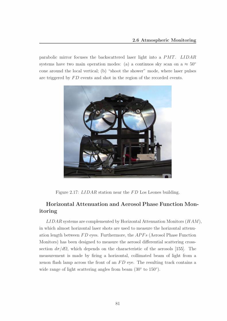
2.6 Atmospheric Monitoring
parabolic mirror focuses the backscattered laser light into a PMT . LIDAR
systems have two main operation modes: (a) a continuos sky scan on a ≈ 50
cone around the local vertical; (b) “shoot the shower” mode, where laser pulses
are triggered by FD events and shot in the region of the recorded events.
Figure 2.17: LIDAR station near the FD Los Leones building.
Horizontal Attenuation and Aerosol Phase Function Mon-
itoring
LIDAR systems are complemented by Horizontal Attenuation Monitors (HAM),
in which almost horizontal laser shots are used to measure the horizontal attenu-
ation length between FD eyes. Furthermore, the APFs (Aerosol Phase Function
Monitors) has been designed to measure the aerosol differential scattering cross-
section dσ/dΩ, which depends on the characteristic of the aerosols [155]. The
measurement is made by firing a horizontal, collimated beam of light from a
xenon flash lamp across the front of an FD eye. The resulting track contains a
wide range of light scattering angles from beam (30 to 150).
81
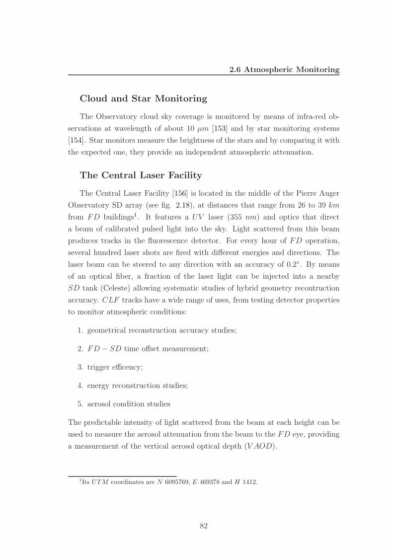
2.6 Atmospheric Monitoring
Cloud and Star Monitoring
The Observatory cloud sky coverage is monitored by means of infra-red ob-
servations at wavelength of about 10 µm [153] and by star monitoring systems
[154]. Star monitors measure the brightness of the stars and by comparing it with
the expected one, they provide an independent atmospheric attenuation.
The Central Laser Facility
The Central Laser Facility [156] is located in the middle of the Pierre Auger
Observatory SD array (see fig. 2.18), at distances that range from 26 to 39 km
from FD buildings1. It features a UV laser (355 nm) and optics that direct
a beam of calibrated pulsed light into the sky. Light scattered from this beam
produces tracks in the fluorescence detector. For every hour of FD operation,
several hundred laser shots are fired with different energies and directions. The
laser beam can be steered to any direction with an accuracy of 0.2. By means
of an optical fiber, a fraction of the laser light can be injected into a nearby
SD tank (Celeste) allowing systematic studies of hybrid geometry recontruction
accuracy. CLF tracks have a wide range of uses, from testing detector properties
to monitor atmospheric conditions:
1. geometrical reconstruction accuracy studies;
2. FD − SD time offset measurement;
3. trigger efficency;
4. energy reconstruction studies;
5. aerosol condition studies
The predictable intensity of light scattered from the beam at each height can be
used to measure the aerosol attenuation from the beam to the FD eye, providing
a measurement of the vertical aerosol optical depth (V AOD).
1Its UTM coordinates are N 6095769, E 469378 and H 1412.
82
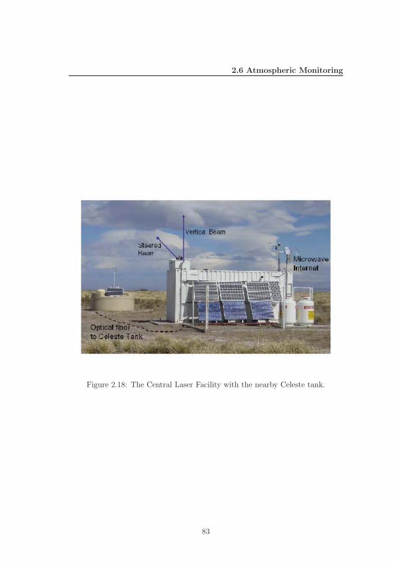
2.6 Atmospheric Monitoring
Figure 2.18: The Central Laser Facility with the nearby Celeste tank.
83
Chapter 3
Event Reconstruction with Pierre
Auger Data
3.1 Introduction
The Auger data acquisition system is based on a hierarchical event trigger, capa-
ble to select interesting events and reject uninteresting ones using event topology
and timing informations. The fluorescence and the surface detectors work inde-
pendently and use two completly independent trigger systems. When both FD
and SD are in operation, event candidates, surviving FD trigger selection, are
sent to the SD data acquisition system, that scans the ground array for triggered
tanks to build up hybrid events.
Recorded events could involve:
1. the only surface array, ordinary SD events (see fig. 3.1);
2. only fluorescence detector, mono FD events if seen by one eye or stereo FD
events if seen by at least two eye (see fig. 3.1);
3. both detectors, hybrid events (see fig. 3.1). Hybrid events could be of differ-
ent kinds: 1 FD eye + 1 SD tank or a few SD tanks, not enough to realize
an independ SD reconstruction; 1 FD eye + n SD tanks, with n higher
enough to perform an independent SD reconstruction (golden events); 2 or
more FD eye + SD informations, stereo-hybrid events (platinum events).
84
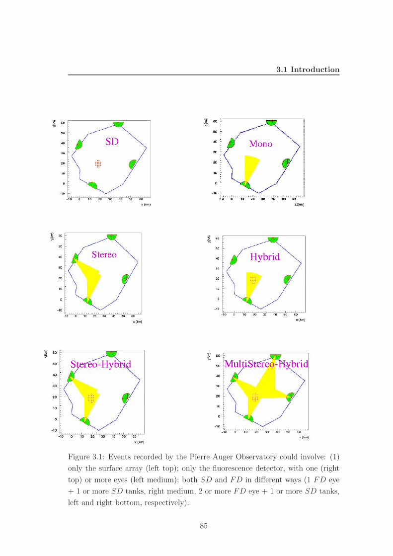
3.1 Introduction
Figure 3.1: Events recorded by the Pierre Auger Observatory could involve: (1)
only the surface array (left top); only the fluorescence detector, with one (right
top) or more eyes (left medium); both SD and FD in different ways (1 FD eye
+ 1 or more SD tanks, right medium, 2 or more FD eye + 1 or more SD tanks,
left and right bottom, respectively).
85
3.2 FD Data Acquisition Strategy
Once the South Observatory will be complete, it is clear that the fraction
of FD only events will be very small, most of FD events will be hybrid (mono
events with a few tanks).
3.2 FD Data Acquisition Strategy
The fluorescence detector trigger is organized upon several levels. There are
two hardware triggers, the first level trigger (FLT ) and the second level trigger
(SLT ), which select pixel above threshold and require a minimum track on the
camera. There are also two software triggers, the third level trigger (TLT ) and
the T3, which operate a noise event rejection and identify event candidates to
send to the Central Data Acquisistion System (CDAS).
FD signals are digitalized by the by flash−ADC every 100 ns (with a fre-
quency of 10 MHz). Analog signals are converted in 16 bit word, whose the
first twelve store the digitized signals and the latter 4 are control bits (like the
status bit, which says if the pixel is above the threshold, ON , or not, OFF ). Sig-
nal words are stored in a 32 K SRAM memory till a second level trigger signal
occours.
3.2.1 First Level Trigger
The first level trigger is the pixel level trigger. It selects PMT tubes which
are above a threshold. The system distinguishes fluorescence light from night
sky background photons by means of a logic based on a running sum of the
last 10 digitized FADC values [157]. The result of the sum is compared with
a programmable trigger threshold. The threshold automatically varies to hold a
fix trigger rate of 100 Hz, independently pixel by pixel. This system takes into
account for any variation during an acquisition night due to electronics problems
or light background (bright stars in the field of view, etc.). A pixel above the
threshold is labelled as ON and holds its status for 20 µs once the running sum
on its signal has fallen below the threshold.
86
3.2 FD Data Acquisition Strategy
3.2.2 Second Level Trigger
The second level trigger is based upon a pattern recognition procedure on FLT
pixels.
Patterns to look for are defined from a set of five basic configuration of five
pixel each (see fig. 3.2). The complete set of valid patterns is obtained by means
of a rotation of 60 and 120 and by reflection with respect to x and y axis.
Patterns obtained are 39, but for the hexagonal system simmetry one should
consider separately patterns for odd and even rows, the possible configurations
are 78. Requiring only 4 FLT pixels of 5−pixel pattern 1, the list of possible
patterns grows up to 108, leaving out equivalent configurations. The procedure
takes 1 µs to perform a complete scan of the camera. The scan proceeds column
by column, taking for each one a 20 × 5 pixel matrix. In the latter sub-matrix,
the SLT tests possible patterns associated with triggered pixels.
Once a track is compatible with a reference pattern, a SLT signal is issued.
The event is held in the memory till it is processed by the following trigger level.
The memory has a capacity of 32 events. The SLT rate is below 1 Hz for each
telescope.
3.2.3 Third Level Trigger
The first FD software trigger is the TLT . The TLT manages the event readout
and applies a noise rejection algorithm. For events passing the noise rejection
algorithm, a list of triggered pixels and their closest neighbours (to avoid any
signal losses) is compiled. At the end, the complete event data is stored in
an event file. If the event data are coming from more than one mirror, the
TLT integrates it in a single event structure, eye-event structure. Now the data
contain:
1. FLT data, FLT pixels, at what time and how long they are above threshold.
1In this way it is possible to take into account pixels fired marginally or with some hardwareproblem.
87
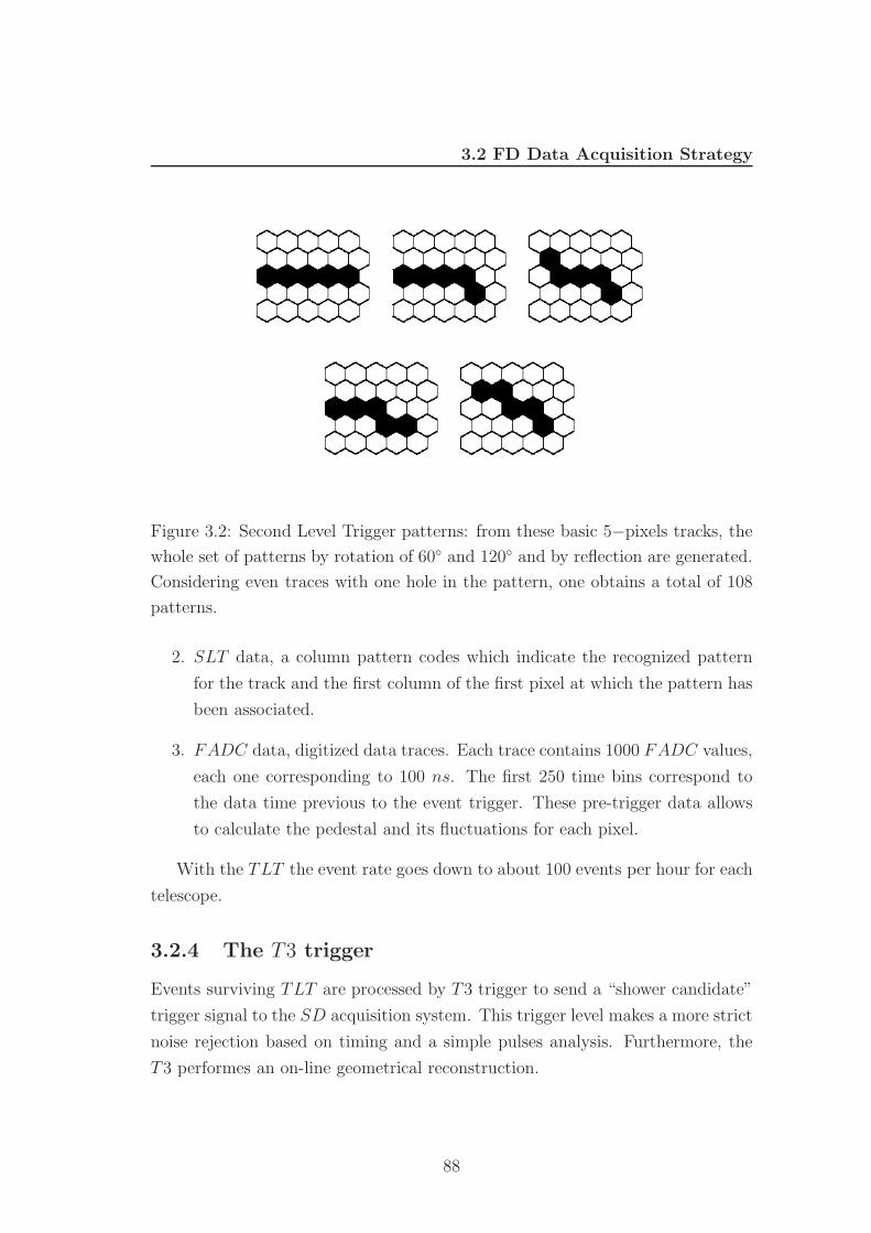
3.2 FD Data Acquisition Strategy
Figure 3.2: Second Level Trigger patterns: from these basic 5−pixels tracks, the
whole set of patterns by rotation of 60 and 120 and by reflection are generated.
Considering even traces with one hole in the pattern, one obtains a total of 108
patterns.
2. SLT data, a column pattern codes which indicate the recognized pattern
for the track and the first column of the first pixel at which the pattern has
been associated.
3. FADC data, digitized data traces. Each trace contains 1000 FADC values,
each one corresponding to 100 ns. The first 250 time bins correspond to
the data time previous to the event trigger. These pre-trigger data allows
to calculate the pedestal and its fluctuations for each pixel.
With the TLT the event rate goes down to about 100 events per hour for each
telescope.
3.2.4 The T3 trigger
Events surviving TLT are processed by T3 trigger to send a “shower candidate”
trigger signal to the SD acquisition system. This trigger level makes a more strict
noise rejection based on timing and a simple pulses analysis. Furthermore, the
T3 performes an on-line geometrical reconstruction.
88
3.3 SD Trigger and Data Selection
Shower candidates are identified by looking for events with finite pulse widths
and finite transit times between PMT (shower front is moving in the field of view
if the detector), which depend on shower energy and geometry.
Rejected events could be due to: accidental triggers, small track and no signal
in the triggered pixels; coherent noise, usually associated with weather condi-
tions (lightning and storms in the field of view), characterized by noise signals
distributed almost over all the camera; cosmic ray hitting directly the detector,
high and short pulses and negligible transit times among pixels.
Usign the pixel list coming from SLT , T3 operates a fast signal analysis, based
on searching the FADC trace maximum. Then the noise rejection algorithm is
applied.
The system makes in two steps an on-line reconstruction: a fit to a track on
the camera, to determine the plane containing almost all triggered pixel pointing
direction (the so called shower detector plane SDP ) and so its projection on the
ground (landing line); a time fit on pixel timing and their observation angles to
estimate the expected arrival time for light emitted by shower front at ground
level (landing time).
The resulting T3 trigger rate is between 5 and 10 shower candidates per hour
for each telescope.
3.3 SD Trigger and Data Selection
Cerenkov photons produced by shower front secondary particles traversing the
SD tank, are recorded by three downward facing PMTs (see sec. 2.4). A low
and high gain signal from each photmultiplier is sent to front-end electronics.
High gain signal is evaluated every 25 ns by the trigger/memory circuitry for
interesting patterns, which stores the data in a buffer memory and informs the
detector station micro-controller when a trigger occurs.
Surface detector trigger levels have a similar hierarchical design structure of
those of the fluorescence detector. The trigger system has been designed to allow
the ground array to operate at a wide range of primary energies, for vertical and
very inclined showers, with a full efficiency for primary particles above 1019 eV .
89
3.3 SD Trigger and Data Selection
There are two trigger levels implemented directly at tank level, T1 and T2. A
further trigger level, T3, is formed at observatory campus based upon the spatial
and temporal correlation of the 2 level triggers. All data surviving T3 are stored.
Additional trigger levels are implemented in order to select physical events (T4,
physics trigger) and accurate events (T5, quality trigger).
3.3.1 Tank Level Triggers
The trigger/memory circuitry produces a first level trigger based upon hardware
analysis of the high gain PMT signals. The T1 uses two important shower
waveform properties: 1) on average, for any fixed number of Cerenkov photons
detected, those from higher energy showers will be more spread out in time with
respect to those from lower energy showers1; 2) signals coming from electrons and
photons are usually smaller than those of muons2.
At tank level, the T1 uses two different trigger modes:
1. Time over Threshold (ToT ) trigger, which requires that 13 bins in a 120
bins window are above a threshold of 0.2 IestV EM
3 in coincidence on 2 PMT
[159]. This trigger has a rate of about 1.6 Hz. It efficiently selects small
but spread signals, as those coming from high energy distant EAS or low
energy showers, rejecting signals form muon background.
2. 3−fold coincidence of a 1.75 IestV EM threshold. It is more noisy, having a
rate of about 100 Hz, but it is needed to detect fast signals (< 200 ns)
produced by the muonic component of very inclined showers.
T2 is applied in the station controller to select from T1 signals those likely
to have come from EAS and to reduce to 20 Hz the event rate to be sent to the
central station. All of ToT trigger are directly promoted to T2, whereas 3−fold
T1 have to satisfy a higher threshold of 3.2 IestV EM on all of 3 tank’s PMT . The
rate for this trigger level is about 20 Hz.
1A fixed energy contour is farther from shower core in a larger energy showers2At observation level, the energy of muons is usually higher than that of photons and
electrons3The estimated current for a Vertical Equivalent Muon (Iest
V EM ) is the reference unit for thecalibration of FADC signals [160].
90
3.3 SD Trigger and Data Selection
All T2 tanks are used for the hybrid trigger.
3.3.2 Event Selection Triggers
At Observatory campus, the T3 is applied using two different modes:
1. 3 tanks satisfying the ToT conditions and a minimum compactness, that is
one of them must have one of its closest neighbours and one of its second
neighbours triggered. The 90% of events selected by the so called 3ToT are
physical events. It is very efficient for vertical showers.
2. 4−fold coincidence of any T2 with a moderate compactness requirement,
that is among 4 tanks, one can be as far as 6 km away from others within
an appropriate time window. Only 2% of events selected by this mode are
real showers, but it is absolutely needed to detect horizontal showers, which
produce fast signals with a wide-spread topological patterns.
A physical trigger (T4) is needed to select showers from T3 data. For zenith
angles below 60, there is an official physical trigger implemented offline, based on
the compactness of triggered tanks and on the spread in time of FADC traces,
which is enough to satisfy a ToT condition. The present T4 implementation
requires either a compact 3 ToT (see fig. 3.3), which ensures that more than 99%
of selected events are showers, or a compact configuration of any local trigger
called 4C1 (at least one fired station has 3 triggered tanks out of its 6 first
neighbours, see fig. 3.4).
The 3ToT T4 trigger loses less than 5% of showers below 60. The 4C1 trigger,
which event rate is about 2% of the previous one, allows to keep the 5% of the
showers below 60 lost by the former and to select low energy showers above 60.
The definitions of T4 criteria for horizontal showers is still under study [161]
3.3.3 T5 quality Trigger
To compute the detector acceptance and build the spectrum, among events sur-
viving T4 trigger level, only those reconstructed with a known energy and angular
accuracy have been used. Various studies have been performed to identify under
91
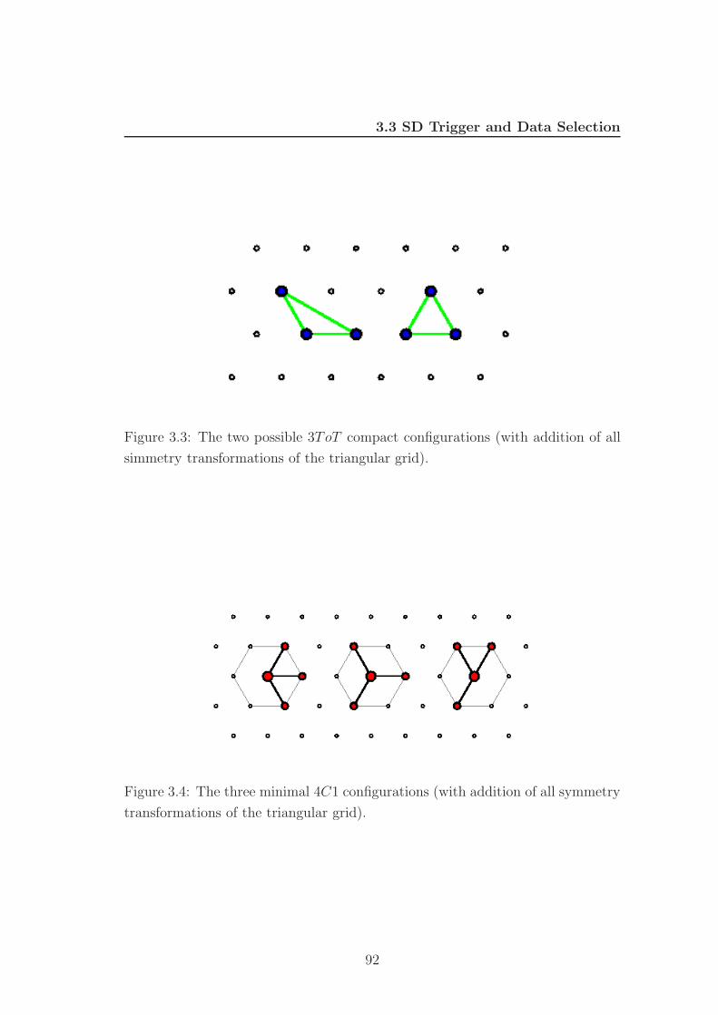
3.3 SD Trigger and Data Selection
Figure 3.3: The two possible 3ToT compact configurations (with addition of all
simmetry transformations of the triangular grid).
Figure 3.4: The three minimal 4C1 configurations (with addition of all symmetry
transformations of the triangular grid).
92
3.4 Hybrid Trigger
which conditions events could satisfy this requirement. This is the task of the
quality trigger (T5).
At moment the T5 implementation requires that the tank with highest sig-
nal must have at least 5 working tanks among its 6 closest neighbours when the
event is recorded. Furthermore, the reconstructed core must be inside an equilat-
eral triangle of working stations. These requirements guarantee that no crucial
informations are missed for shower reconstruction. The study of T5 effects on
reconstruction accuracy and in particular on the signal at 1000 m from the core
(S(1000)) is described in [162]. The maximum systematic uncertainty in the re-
constructed S(1000) due to event sampling into the array or the effect of a missing
internal tank is around 8%.
The total trigger chain allows to reduce the event rate in a single tank from
3 kHz, mainly due to muon background, down to 3 per day, due to real showers,
corresponding to a rejection factor of 108.
3.4 Hybrid Trigger
The main Pierre Auger Observatory feature is its hybrid detection technique:
the possibility to measure the same event by fluorescence and surface detector.
Therefore, in the data acquisition system the hybrid trigger design has a very
important role. In the selected design, the FD T3 signal gives an external trigger
to the surface detector [158]. This choice allows to get hybrid events even with
a single SD station. This is very important, because SD timing information
greatly improves the FD reconstruction, though there is only a single SD tank
data. In fact, the FD axis reconstruction is based upon a minimization of a
function which depends on three parameters (see sec. 3.6.1.2), that determine
the curvature of the pixel time distribution versus their elevation angle. The
timing information coming from the SD introduce new terms in the function
with a different dependence on parameters. So, there will be a fraction of events
that are, in principle, hybrid but that cannot be reconstructed from SD array.
This strategy allows an hybrid reconstruction of low energy events, close to the
FD trigger threshold (E ≥ 3 · 1017 eV ). In fact, this energy range is below the
93
3.5 SD Event Reconstruction
SD trigger threshold but the probability that at least a tank gives a T2 trigger
signal is very high (∼ 100%).
At last FD trigger level, FD events, labelled as shower candidates by T3,
are analyzed on-line and their SDP projection and light arriving time at ground
level are computed. When both SD and FD are in operation, T3 signal and
preliminary reconstruction results are sent to CDAS to trigger the SD. The
landing time and the SDP allow CDAS to calculate the impact time of the
shower front in the SD tank region. Then CDAS looks for compatible SD T2
tanks across the array, with a trigger time within 20 µs of the calculated time.
Triggered tanks, identified by this procedure, are collected and their data are
gathered in an event structure labelled FD−trigger.
Of course, time and resources available to perform on-line reconstruction are
limited, so into T3 software is implemented a semplified version of the more
sophisticated reconstruction methods used for the offline analysis.
In order to not degrade SD trigger performances, T3 signals should arrive to
CDAS within 5 s, that is the maximum SD T2 transit time across the radio
network.
3.5 SD Event Reconstruction
The SD event reconstruction can be schematized in two main steps: the plane
fit, to obtain the geometry of the incident shower, and the lateral distribution fit,
to estimate the energy.
3.5.1 SD Geometry Reconstruction
To calculate the plane fit it is necessary to determine the time window for the
signal, the core on the ground and the shower axis.
A well tested method to fix the time window is to calculate t25 and t50, defined
as the time at which the FADC signal reaches the 25% and the 50% of its
maximum, respectively, to define ts = t25 − 1.5(t50 − t25), and then the start of
the signal is the time t0 at which there is the first FADC count above a fixed
94
3.5 SD Event Reconstruction
threshold, usually 5 photelectrons [139]. To prevent contaminations, the time
window is closed after t50 +K(t50−t0), where K is a parameter to be determined.
Afterwards, one can make a first estimation of the shower core. It comes out
by means of an average of the triggered tank positions, weighting the i−th tank
with its signal Si. If we define a coordinate system for the Observatory, centered
in O, let be b the vector from the origin of the coordinate system to the shower
core and xi the vector from O to the i−th tank, one obtains
b =
∑i Wi xi
Wi(3.1)
where Wi =√
Si.
Then we proceed to the axis determination. We fix the shower core as the
reference point from now on and we associate with it a time T0, worked out from
the weighted average of triggered tank times, as done for the core. For each time
t, the shower front can be represented as a point x(t) moving along the shower
axis a at light velocity, so we can write
x(t) −b = −c(t − T0)a (3.2)
where the versor for the shower axis is pointing toward the source. If we make
the approximation of a flat shower front, the time t at which the front passes
through a point P on the ground, identified by the vector x(t) is given by
ct = cT0 − ( x(t) −b) · a (3.3)
If we assume that there are only the errors associated with the time of triggered
tanks, σt, it is possible to estimate the shower axis minimizing the relation [140]
χ2 =1
σ2t
∑i
[ti − t( xi(t))]2] =
1
c2σ2t
∑i
[cti − cT0 + xi · a]2 (3.4)
where xi, ti and t( xi(t)) are the position and the time measured and expected
for the i−th tank, respectively.
Let be a = (u, v, w), xi = (xi, yi, zi) and cσt = σ, eq. 3.4 becomes
χ2 =1
σ2
∑i
[cti − cT0 + xiu + yiv + ziw]2. (3.5)
95
3.5 SD Event Reconstruction
Minimizing the previous equation, it is possible to get a = (u, v, w), of course
with the condition
u2 + v2 + w2 − 1 = 0. (3.6)
In the above minimization, the error definition plays a leading role. Since
time dispersion increases going away from the core, in the first approximation
quadratically, tanks very far away could cause the failure of this procedure. The
errors are usually defined as a function of the signal. One adopted solution,
derived from simulation studies, is [139]
σi(ns) = 1800/(Si)0.85 (3.7)
where Si is the signal recorded by the i−th tank. If necessary the procedure is
reiterated using a parabolic approximation for the shower front [139].
3.5.2 SD Energy Estimation
The crucial point in the SD event reconstruction is the determination of the
lateral distribution function (LDF ). Each experiment should use an appropri-
ate LDF , which depends on ground array design and characteristics, on shower
zenithal angle and energy and on the primary particle composition, too.
To estimate the primary energy one should phenomenologically find a depen-
dence between the LDF behavior and the shower energy. To do so, one should
massively use shower simulations, in which there are some assumptions and ex-
trapolation on hadronic physics involved. This model-dependence is the Achilles
heel of the SD data analysis.
The dependence of the measured signal S at a distance r from the core is
given by [140]
S(r) = S1000fLDF (r) (3.8)
where fLDF (r) is the lateral distribution function and S1000 is the signal measured
at r = 1000 m from the core. Of corse the LDF has the normalization condition
fLDF (r) = 1. The signal uncertainty is assumed as [141]
σS = 1.06√
S (3.9)
96
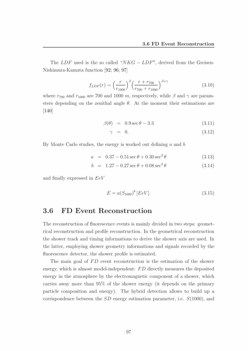
3.6 FD Event Reconstruction
The LDF used is the so called “NKG − LDF ′′, derived from the Greisen-
Nishimura-Kamata function [92; 96; 97]
fLDF (r) =( r
r1000
)β( r + r700
r700 + r1000
)β+γ
(3.10)
where r700 and r1000 are 700 and 1000 m, respectively, while β and γ are param-
eters depending on the zenithal angle θ. At the moment their estimations are
[140]
β(θ) = 0.9 sec θ − 3.3 (3.11)
γ = 0. (3.12)
By Monte Carlo studies, the energy is worked out defining a and b
a = 0.37 − 0.51 sec θ + 0.30 sec2 θ (3.13)
b = 1.27 − 0.27 sec θ + 0.08 sec2 θ (3.14)
and finally expressed in EeV
E = a(S1000)b [EeV ]. (3.15)
3.6 FD Event Reconstruction
The reconstruction of fluorescence events is mainly divided in two steps: geomet-
rical reconstruction and profile reconstruction. In the geometrical reconstruction
the shower track and timing informations to derive the shower axis are used. In
the latter, employing shower geometry informations and signals recorded by the
fluorescence detector, the shower profile is estimated.
The main goal of FD event reconstruction is the estimation of the shower
energy, which is almost model-independent: FD directly measures the deposited
energy in the atmosphere by the electromagnetic component of a shower, which
carries away more than 95% of the shower energy (it depends on the primary
particle composition and energy). The hybrid detection allows to build up a
corrispondence between the SD energy estimation parameter, i.e. S(1000), and
97
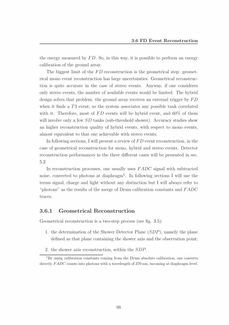
3.6 FD Event Reconstruction
the energy measured by FD. So, in this way, it is possible to perform an energy
calibration of the ground array.
The biggest limit of the FD reconstruction is the geometrical step: geomet-
rical mono event reconstruction has large uncertainties. Geometrical reconstruc-
tion is quite accurate in the case of stereo events. Anyway, if one consideres
only stereo events, the number of available events would be limited. The hybrid
design solves that problem: the ground array receives an external trigger by FD
when it finds a T3 event, so the system associates any possible tank correlated
with it. Therefore, most of FD events will be hybrid event, and 60% of them
will involve only a few SD tanks (sub-threshold shower). Accuracy studies show
an higher reconstruction quality of hybrid events, with respect to mono events,
almost equivalent to that one achievable with stereo events.
In following sections, I will present a review of FD event reconstruction, in the
case of geometrical reconstruction for mono, hybrid and stereo events. Detector
reconstruction performances in the three different cases will be presented in sec.
5.2.
In reconstruction processes, one usually uses FADC signal with subtracted
noise, converted to photons at diaphragm1. In following sections I will use the
terms signal, charge and light without any distinction but I will always refer to
“photons” as the results of the merge of Drum calibration constants and FADC
traces.
3.6.1 Geometrical Reconstruction
Geometrical reconstruction is a two-step process (see fig. 3.5):
1. the determination of the Shower Detector Plane (SDP ), namely the plane
defined as that plane containing the shower axis and the observation point;
2. the shower axis reconstruction, within the SDP .
1By using calibration constants coming from the Drum absolute calibration, one convertsdirectly FADC counts into photons with a wavelength of 370 nm, incoming at diaphragm level.
98
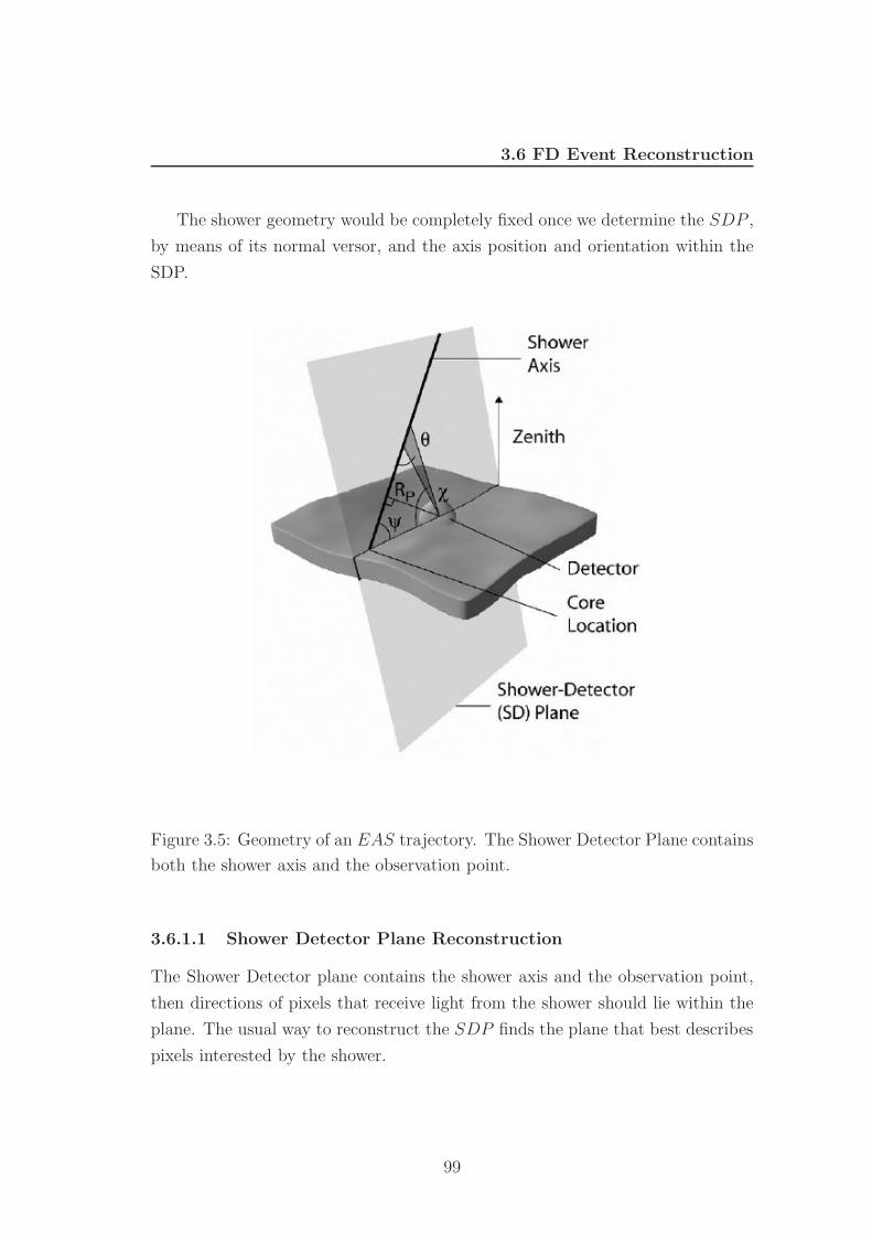
3.6 FD Event Reconstruction
The shower geometry would be completely fixed once we determine the SDP ,
by means of its normal versor, and the axis position and orientation within the
SDP.
Figure 3.5: Geometry of an EAS trajectory. The Shower Detector Plane contains
both the shower axis and the observation point.
3.6.1.1 Shower Detector Plane Reconstruction
The Shower Detector plane contains the shower axis and the observation point,
then directions of pixels that receive light from the shower should lie within the
plane. The usual way to reconstruct the SDP finds the plane that best describes
pixels interested by the shower.
99
3.6 FD Event Reconstruction
The SDP normal vector, n is found minimizing:
χ2 =∑
i
(ri · n) · wi (3.16)
where ri is pointing direction of the i−th PMT and wi is a weight proportional
to its signal. The sum runs over all triggered pixels. Using SDP reconstruction,
it is possible to discard triggered pixels away from the fit.
3.6.1.2 Shower Axis Reconstruction
The second reconstruction step is the determination of the shower axis within
the SDP . The shower axis is estimated using the timing information from FD
signals. As already said, events could involve the ground array and the fluo-
rescence detector in different ways producing mono, hybrids, stereo and stereo-
hybrid events. In this reconstruction step one can use additional informations
from the ground array or by different eyes when they are available, to improve
reconstruction performances.
Mono Reconstruction
In the SDP plane, we can define RP , χ0 and T0 as the minimum distance
between the axis and the observation point (impact parameter), the angle between
the trajectory and the horizontal plane, passing from the detector, within the
SDP , and the time at which the shower front plane passes through the detector
center, respectively (see fig. 3.5 and fig. 3.6).
So, the light reaching the PMT at time ti from any point with viewing angle
θi is delayed from the arrival time T0. The delayed time is
δt(θi) = tiT0 =RP
c sinθi− RP
c tanθi=
RP tan(θi/2)
c(3.17)
where c is the speed of light, ti is the i−th tube trigger time and θi is related
to χ0 by
θi = χ0 − χi (3.18)
where χi is the tube elevation angle in the plane (see fig. 3.6).
100
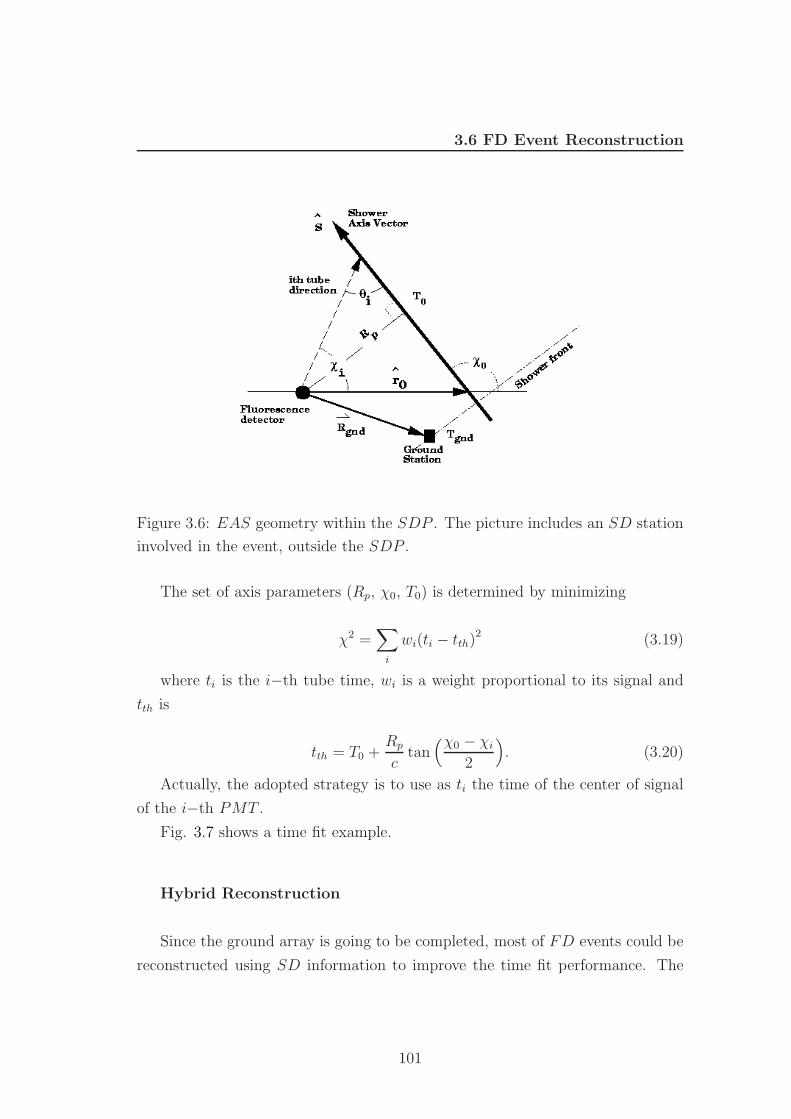
3.6 FD Event Reconstruction
Figure 3.6: EAS geometry within the SDP . The picture includes an SD station
involved in the event, outside the SDP .
The set of axis parameters (Rp, χ0, T0) is determined by minimizing
χ2 =∑
i
wi(ti − tth)2 (3.19)
where ti is the i−th tube time, wi is a weight proportional to its signal and
tth is
tth = T0 +Rp
ctan
(χ0 − χi
2
). (3.20)
Actually, the adopted strategy is to use as ti the time of the center of signal
of the i−th PMT .
Fig. 3.7 shows a time fit example.
Hybrid Reconstruction
Since the ground array is going to be completed, most of FD events could be
reconstructed using SD information to improve the time fit performance. The
101
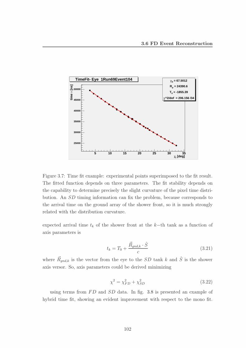
3.6 FD Event Reconstruction
[deg]iχ5 10 15 20 25 30 35
[n
s]×
tim
e
25000
30000
35000
40000
45000
50000
= 67.50120χ
= 24390.6pR
= -1855.390T
^2/dof = 206.156 /34χ
TimeFit- Eye 1Run69Event104
Figure 3.7: Time fit example: experimental points superimposed to the fit result.
The fitted function depends on three parameters. The fit stability depends on
the capability to determine precisely the slight curvature of the pixel time distri-
bution. An SD timing information can fix the problem, because corresponds to
the arrival time on the ground array of the shower front, so it is much strongly
related with the distribution curvature.
expected arrival time tk of the shower front at the k−th tank as a function of
axis parameters is
tk = T0 +Rgnd,k · S
c(3.21)
where Rgnd,k is the vector from the eye to the SD tank k and S is the shower
axis versor. So, axis parameters could be derived minimizing
χ2 = χ2FD + χ2
SD (3.22)
using terms from FD and SD data. In fig. 3.8 is presented an example of
hybrid time fit, showing an evident improvement with respect to the mono fit.
102
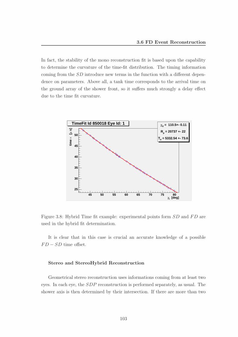
3.6 FD Event Reconstruction
In fact, the stability of the mono reconstruction fit is based upon the capability
to determine the curvature of the time-fit distribution. The timing information
coming from the SD introduce new terms in the function with a different depen-
dence on parameters. Above all, a tank time corresponds to the arrival time on
the ground array of the shower front, so it suffers much strongly a delay effect
due to the time fit curvature.
[deg]iχ45 50 55 60 65 70 75 80
s]
µ
[×
tim
e
25
30
35
40
45
50
= 110.5+- 0.110χ
= 20737 +- 22pR
= 5332.54 +- 73.60T
TimeFit Id 850018 Eye Id: 1
Figure 3.8: Hybrid Time fit example: experimental points form SD and FD are
used in the hybrid fit determination.
It is clear that in this case is crucial an accurate knowledge of a possible
FD − SD time offset.
Stereo and StereoHybrid Reconstruction
Geometrical stereo reconstruction uses informations coming from at least two
eyes. In each eye, the SDP reconstruction is performed separately, as usual. The
shower axis is then determined by their intersection. If there are more than two
103
3.6 FD Event Reconstruction
eyes involved1, one should select eyes whose SDP versors ni and nj have the
lowest scalar product module. The selection should consider only SDP recon-
structed with a good accuracy. With this procedure, only geometrical parameters
of the shower axis are determined. T0 is estimated minimizing the usual time fit
formula or that one used in hybrid case, if the event is also hybrid, but fixing Rp,
χ0 and S. In principle, T0 estimation could be done for both eye used to fix the
shower axis2. Its final value will be the weighted mean of this two estimation.
3.6.2 Longitudinal Profile Reconstruction
In order to extract physical information from recorded data, once the shower ge-
ometry has been reconstructed, it is possible to determine the shower longitudinal
development. To perform the reconstruction of the shower longitudinal profile,
we proceed in three reconstruction steps:
1. Determination of the light profile, that is the number of photons reach-
ing the detector at diaphragm each FADC time bin. For each FADC time
bin ti, we consider the expected direction from which the fluorescence light
is coming from, given by the vector Ri pointing from the eye to the shower
axis and forming an angle χi with the horizontal plane within the SDP
calculated from
χi = χ0 − 2 tan( c
Rp
(ti − T0))
(3.23)
inverting eq. 3.17. Then, the total charge recorded by FD telescopes is
computed, summing over all pixels, triggered and not, whose angle between
their pointing directions and Ri is lower than a value ζ . The value of
the parameter ζ is dynamically computed, event by event, maximizing the
signal to noise ratio over all the light profile. The result is the determination
of the light profile reaching the detector as a function of time (see fig:3.9).
1In august 2005, for the first time a 3−eyes event has been recorded. From that date, a 4tri-ocular event has been recorded
2One of two involved eyes in a stereo event could have recorded a short track of 5−7 pixels,which are enough to estimate an SDP but not to perform the time fit.
104
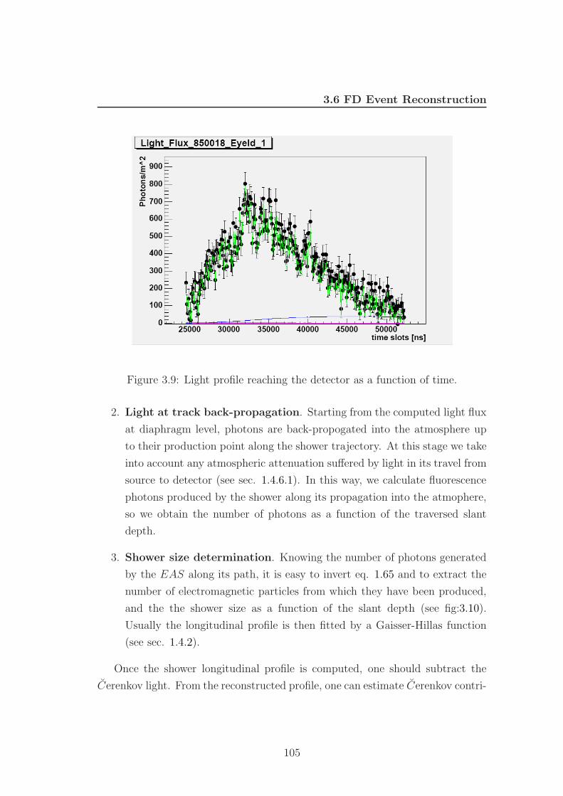
3.6 FD Event Reconstruction
Figure 3.9: Light profile reaching the detector as a function of time.
2. Light at track back-propagation. Starting from the computed light flux
at diaphragm level, photons are back-propogated into the atmosphere up
to their production point along the shower trajectory. At this stage we take
into account any atmospheric attenuation suffered by light in its travel from
source to detector (see sec. 1.4.6.1). In this way, we calculate fluorescence
photons produced by the shower along its propagation into the atmophere,
so we obtain the number of photons as a function of the traversed slant
depth.
3. Shower size determination. Knowing the number of photons generated
by the EAS along its path, it is easy to invert eq. 1.65 and to extract the
number of electromagnetic particles from which they have been produced,
and the the shower size as a function of the slant depth (see fig:3.10).
Usually the longitudinal profile is then fitted by a Gaisser-Hillas function
(see sec. 1.4.2).
Once the shower longitudinal profile is computed, one should subtract the
Cerenkov light. From the reconstructed profile, one can estimate Cerenkov contri-
105
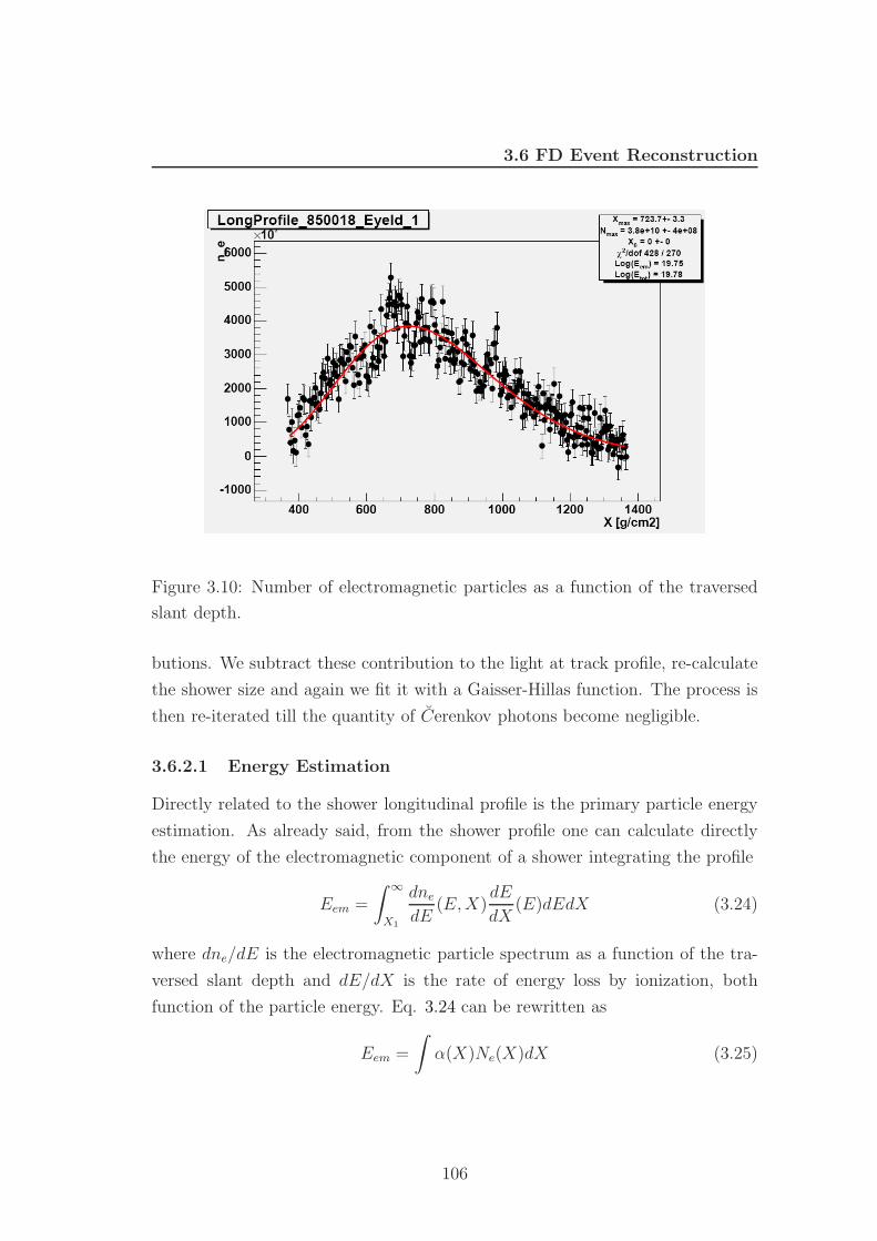
3.6 FD Event Reconstruction
Figure 3.10: Number of electromagnetic particles as a function of the traversed
slant depth.
butions. We subtract these contribution to the light at track profile, re-calculate
the shower size and again we fit it with a Gaisser-Hillas function. The process is
then re-iterated till the quantity of Cerenkov photons become negligible.
3.6.2.1 Energy Estimation
Directly related to the shower longitudinal profile is the primary particle energy
estimation. As already said, from the shower profile one can calculate directly
the energy of the electromagnetic component of a shower integrating the profile
Eem =
∫ ∞
X1
dne
dE(E, X)
dE
dX(E)dEdX (3.24)
where dne/dE is the electromagnetic particle spectrum as a function of the tra-
versed slant depth and dE/dX is the rate of energy loss by ionization, both
function of the particle energy. Eq. 3.24 can be rewritten as
Eem =
∫α(X)Ne(X)dX (3.25)
106
3.6 FD Event Reconstruction
where
α(X) =1
Ne
∫ ∞
X1
dne
dE(E, X)
dE
dX(E)dE (3.26)
is the mean ionization loss rate per shower particle at depth X. α(X) is
only slightly dependent on X, in particular in the initial stage of the shower
development, where the number of electromagnetic particles is relatively small.
It is possible to consider the function as a constant with a value of about 2.19
MeV/(g/cm2) as derived in [163]. This point is a potential source of systematic
effects.
To infer the shower total energy E, it is possible to use a recent parametriza-
tion [163] of the unseen energy in terms of Eem in 1018 eV units
Eem
E= 0.959 − 0.082E−0.150
em (3.27)
obtained averaging over corrections for proton and iron primaries. This aver-
age introduces a 5% energy uncertainty. This correction is clearly not applicable
to a case of a pure electromagnetic shower, which profile is not described by
a Gaisser-Hillas parametrization as well as that one coming from an hadronic
shower.
3.6.3 Systematic Uncertainties
There are several sources of uncertainties in the energy reconstruction of an FD
event. The sources the most important are:
1. Absolute telescope calibration ∼ 12%. This value is mainly due to the
calibration of the drum itself. In the near future it could be reduced to 7%.
2. Fluorescence yield ∼ 10% systematic and ∼ 3% statistical uncer-
tainties [127]. Actually, in order to obtain a much better precision, a new
set of measurements is going to be performed [164].
3. Atmospheric Modeling ∼ 30 g/cm2 on Xmax determination. for
inclined showers [150]. Errors in the knowledge of atmospheric density
profiles introduce systematic error into slant depth calculation. Of course,
the error depends on shower zenith angle. Effects on fluorescence yield
107
3.7 The Offline Software Framework of the Pierre Auger Observatory
and Rayleigh transmission are negligible compared with their systematic
uncertainties.
4. Mie scattering ∼ 15% and ∼ 10 g/cm2 on Xmax estimation [165] (see
sec. 1.4.6.1). Aerosol light absorbption plays an important role in the pro-
file reconstruction. The concentration and the composition of atmospheric
aerosol is highly variable even on short time scales. Their effects depend
event on shower geometry. A large amount of work have been done by the
Pierre Auger Collaboration on atmospheric monitoring.
5. Unseen Energy ∼ 5%. It depends on the primary mass. As already
explained, the parametrization used is obtained averaging over proton and
iron primary particles.
6. Other Effects. There are further sources of systematic uncertainties like
the model dependence of Cerenkov calculations or in the electromagnetic
energy integration.
Of course, any systematic effect in the geometric reconstruction will induce a
systematic effect into shower profile reconstruction.
3.7 The Offline Software Framework of the Pierre
Auger Observatory
Within the Pierre Auger Collaboration, a general purpose software Framework
[167] has been designed in order to implement algorithms and configuration in-
structions to build the variety of applications required by event simulation and
reconstruction tasks.
The framework is flexible as well as robust to support the collaborative effort
of a large number of physicists developing a variety of applications over a 20 year
experimental run. It is able to handle different data formats in order to deal with
event, monitoring informations and air shower simulation code outputs.
The framework is implemented in C++ and takes advantage of object oriented
design and common open source tools, while keeping the user-side simple enough
108
3.7 The Offline Software Framework of the Pierre Auger Observatory
for C + + novice to learn in a reasonable time. Code implementation has taken
place over the last two years and it is now being employed in analysis of data
gathered by the observatory.
The Offline framework comprises three principal part:
1. a collection of processing modules which can be assembled and sequenced
through instructions provided in an XML file [168];
2. an event structure through which modules can relate all pieces of experi-
mental information and which accumulates all simulation and reconstruc-
tion results;
3. a detector description which provides a gateway to data describing the
configuration and performance of the observatory as well as atmospheric
conditions as a function of time.
Processing algorithms, developed by the Collaboration, can be inserted in so-
called modules, which can be put together defining an analysis Module Sequence
by means of an XML file. This modular design allows to easily exchange code,
compare algorithms and build up a variety of applications by combining modules
in various sequences.
Cuts, parameters and configuration instructions used by modules or by the
framework itself are stored in XML files.
The Offline is built on a collection of utilities, including a XERCES−based
[170] parser, an error logger and a set foundation classes to represent objects
such as signal traces, tabulated functions and particles. The utilities collection
also provides a geometry package in which objects such as vectors and points keep
track of the coordinate system in which they are represented. This allows for their
abstract manipulation, as any coordinate trasformation which may be required in
an operation between objects is automatically performed. The geometry package
also includes support for geodetic coordinates.
The event data structure contains all raw, calibrated, reconstructed and Monte
Carlo data and acts as the principale backbone for comunication between mod-
ules. The event structure is built up dynamically as needed and is instrumented
109
3.7 The Offline Software Framework of the Pierre Auger Observatory
with functions allowing modules to interrogate the event at any point to discover
its current constituents.
The detector description provides an intuitive interface from which module
authors may retrieve information about the detector configuration and perfor-
mance. The interface is organized following the hierarchy normally associated
with the observatory instruments. Generally, static detector informations are
stored in XML files, while time-varying monitoring and calibration data are
stored in MySQL [169] databases.
110
Chapter 4
Application of Gnomonic
Projection to the SDP
reconstruction for FD events
4.1 Introduction
In this chapter I will describe a new approach to the Shower Detector Plane
reconstruction of FD events, developed by myself in collaboration with the Auger
Napoli group. This work has the aim to offer an alternative approach to the
problem of SDP finding.
The first step to be performed in the reconstruction of FD events is the de-
termination of the Shower Detector Plane, defined as the plane containing the
shower axis and the center of the FD detector. The accuracy of this procedure is
crucial for a reliable reconstruction of both mono and stereo events.
The strategy adopted in the SDP determination process is based on the idea
that shower track images, as seen by the fluorescence detector, are great circles
on the surface of FD cameras. Great circles can be projected to a straight line on
the tangent plane to the spherical surface of the camera by means of a gnomonic
projection. This line is on the SDP plane, then the problem of SDP finding is
reduced to a track finding and to a a least squares linear fit to the projected
coordinates derived by pixel pointing directions.
111
4.2 Reconstruction strategy
The procedure I propose has been fully implemented in the Auger Offline
Analysis framework and is based on a robust analytical treatment of projections
and fitting.
In order to study the performances of this approach, a wide set of simulated
showers has been produced and analysed. The angular resolution on the recon-
structed SDP has been studied as a function of shower energy and distance, and
compared with the results obtained with the standard Offline reconstruction.
Results show that the gnomonic algorithm appears to be more stable and
accurate, especially for showers with large core distances from the FD detector.
Then the effect of the improved SDP reconstruction on the determination of the
shower axis, energy and longitudinal profile is discussed.
In the following I describe the reconstruction strategy and make a detailed
comparison of the performances of this approach with the standard Auger Offline
framework reconstruction.
4.2 Reconstruction strategy
The default version of the SDP reconstruction module in the Offline Framework
defines the SDP plane as the plane that minimizes the sum of the scalar products
of the vector normal to the trial SDP plane and the direction of single triggered
pixels, as explained in sec. 3.6.1.1.
In order to be able to define data, different from single pixel directions, to
be used in the reconstruction, a few changes were made to the offline framework
that allowed us to add a pixel selection and a “coordinate” definition module.
A default module for coordinate definition is also provided, that simply returns
directions, charges and the times of the barycentre of the reconstructed pulse
for the pixels. The default SDP reconstruction module was modified to access
these data. With this choice the present default Offline Framework reconstruction
chain is unchanged, but I added the possibility to the user to define his own input
data to the algorithm as discussed in section 4.2.2. Furthermore, I implemented
a module for making a pixel pre-selection before the SDP finding process.
112
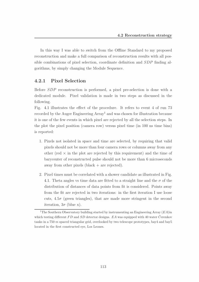
4.2 Reconstruction strategy
In this way I was able to switch from the Offline Standard to my proposed
reconstruction and make a full comparison of reconstruction results with all pos-
sible combinations of pixel selection, coordinate definition and SDP finding al-
gorithms, by simply changing the Module Sequence.
4.2.1 Pixel Selection
Before SDP reconstruction is performed, a pixel pre-selection is done with a
dedicated module. Pixel validation is made in two steps as discussed in the
following.
Fig. 4.1 illustrates the effect of the procedure. It refers to event 4 of run 73
recorded by the Auger Engineering Array1 and was chosen for illustration because
it is one of the few events in which pixel are rejected by all the selection steps. In
the plot the pixel position (camera row) versus pixel time (in 100 ns time bins)
is reported:
1. Pixels not isolated in space and time are selected, by requiring that valid
pixels should not be more than four camera rows or columns away from any
other (red × in the plot are rejected by this requirement) and the time of
barycenter of reconstructed pulse should not be more than 6 microseconds
away from other pixels (black + are rejected).
2. Pixel times must be correlated with a shower candidate as illustrated in Fig.
4.1. Theta angles vs time data are fitted to a straight line and the σ of the
distribution of distances of data points from fit is considered. Points away
from the fit are rejected in two iterations: in the first iteration I use loose
cuts, 4.5σ (green triangles), that are made more stringent in the second
iteration, 3σ (blue x).
1The Southern Observatory building started by instrumenting an Engineering Array (EA)inwhich testing different FD and SD detector designs. EA was equipped with 40 water Cerenkovtanks in a 750 m spaced triangular grid, overlooked by two telescope prototypes, bay4 and bay5located in the first constructed eye, Los Leones.
113
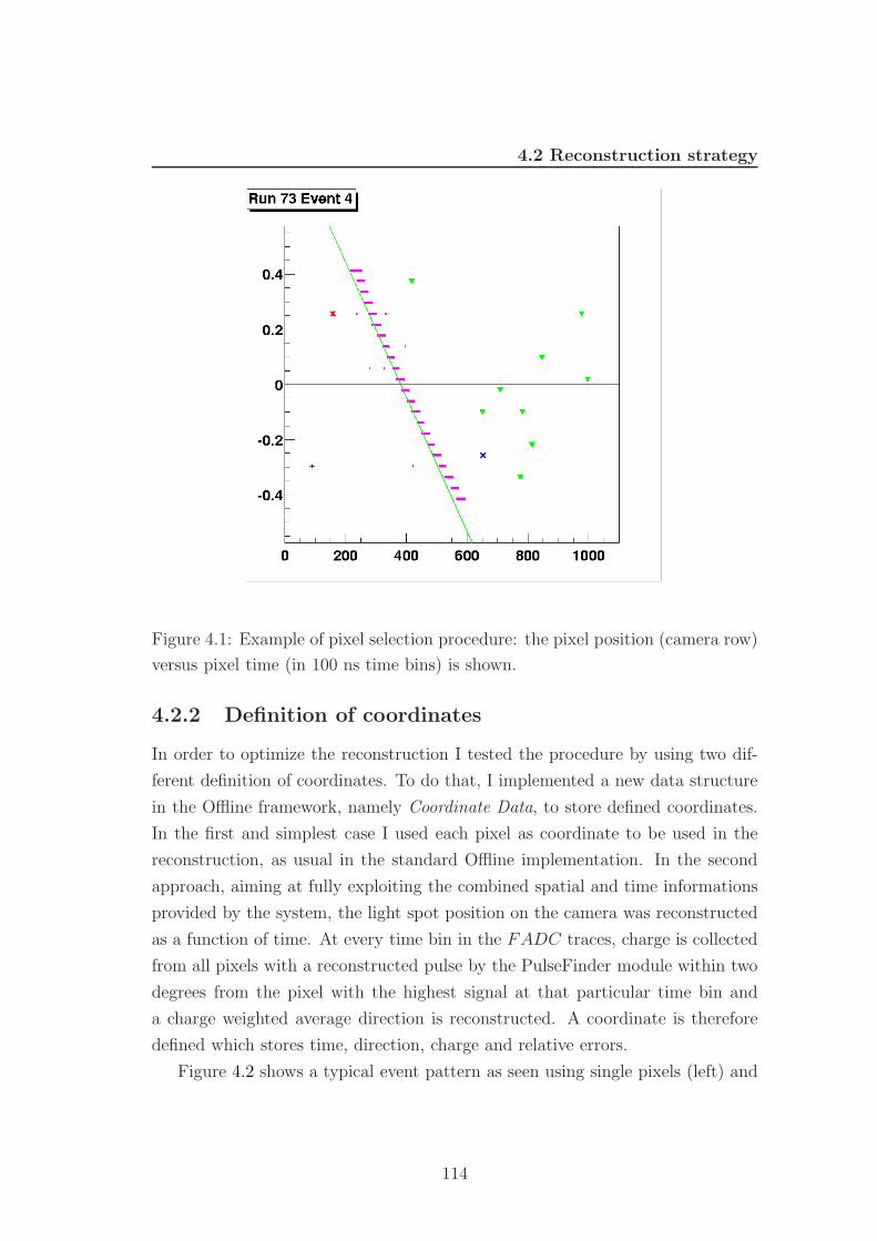
4.2 Reconstruction strategy
Figure 4.1: Example of pixel selection procedure: the pixel position (camera row)
versus pixel time (in 100 ns time bins) is shown.
4.2.2 Definition of coordinates
In order to optimize the reconstruction I tested the procedure by using two dif-
ferent definition of coordinates. To do that, I implemented a new data structure
in the Offline framework, namely Coordinate Data, to store defined coordinates.
In the first and simplest case I used each pixel as coordinate to be used in the
reconstruction, as usual in the standard Offline implementation. In the second
approach, aiming at fully exploiting the combined spatial and time informations
provided by the system, the light spot position on the camera was reconstructed
as a function of time. At every time bin in the FADC traces, charge is collected
from all pixels with a reconstructed pulse by the PulseFinder module within two
degrees from the pixel with the highest signal at that particular time bin and
a charge weighted average direction is reconstructed. A coordinate is therefore
defined which stores time, direction, charge and relative errors.
Figure 4.2 shows a typical event pattern as seen using single pixels (left) and
114
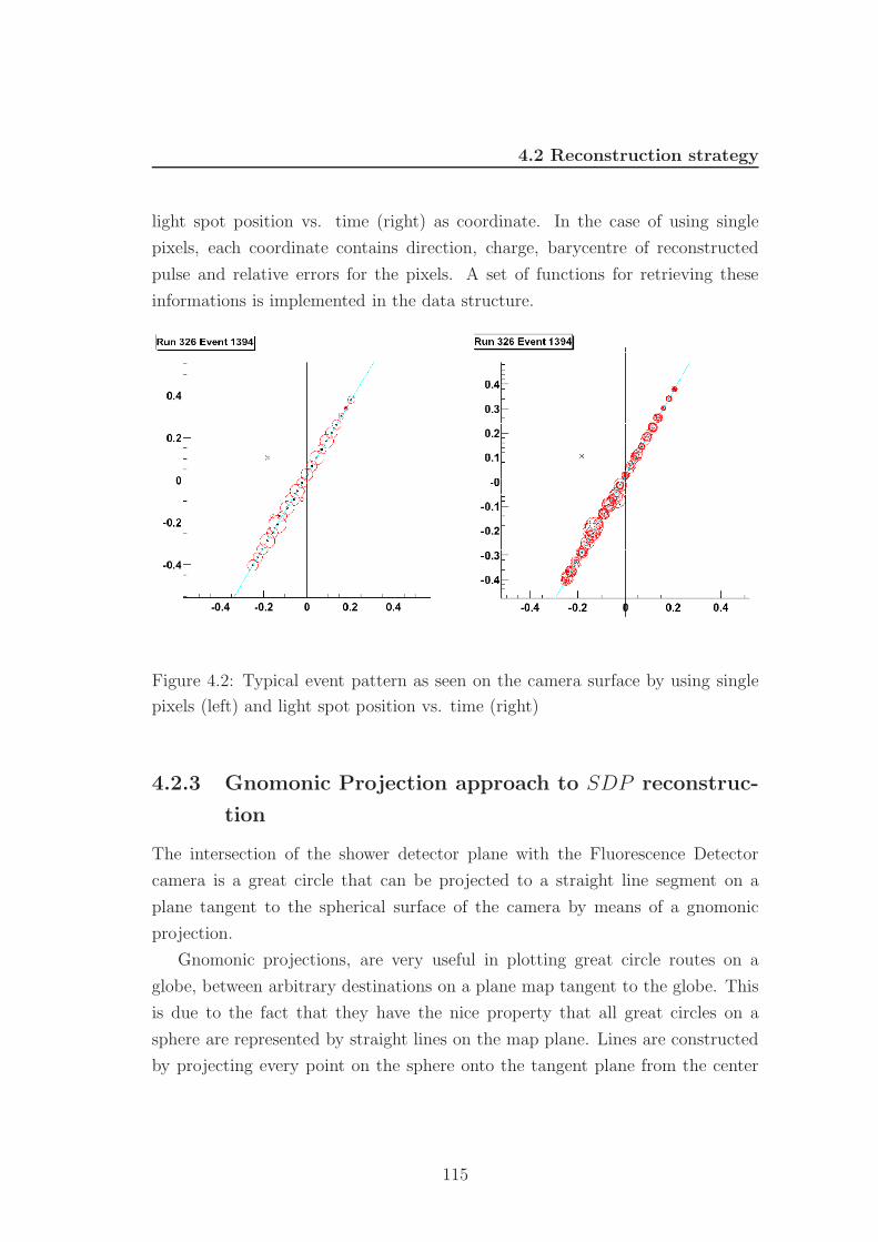
4.2 Reconstruction strategy
light spot position vs. time (right) as coordinate. In the case of using single
pixels, each coordinate contains direction, charge, barycentre of reconstructed
pulse and relative errors for the pixels. A set of functions for retrieving these
informations is implemented in the data structure.
Figure 4.2: Typical event pattern as seen on the camera surface by using single
pixels (left) and light spot position vs. time (right)
4.2.3 Gnomonic Projection approach to SDP reconstruc-
tion
The intersection of the shower detector plane with the Fluorescence Detector
camera is a great circle that can be projected to a straight line segment on a
plane tangent to the spherical surface of the camera by means of a gnomonic
projection.
Gnomonic projections, are very useful in plotting great circle routes on a
globe, between arbitrary destinations on a plane map tangent to the globe. This
is due to the fact that they have the nice property that all great circles on a
sphere are represented by straight lines on the map plane. Lines are constructed
by projecting every point on the sphere onto the tangent plane from the center
115
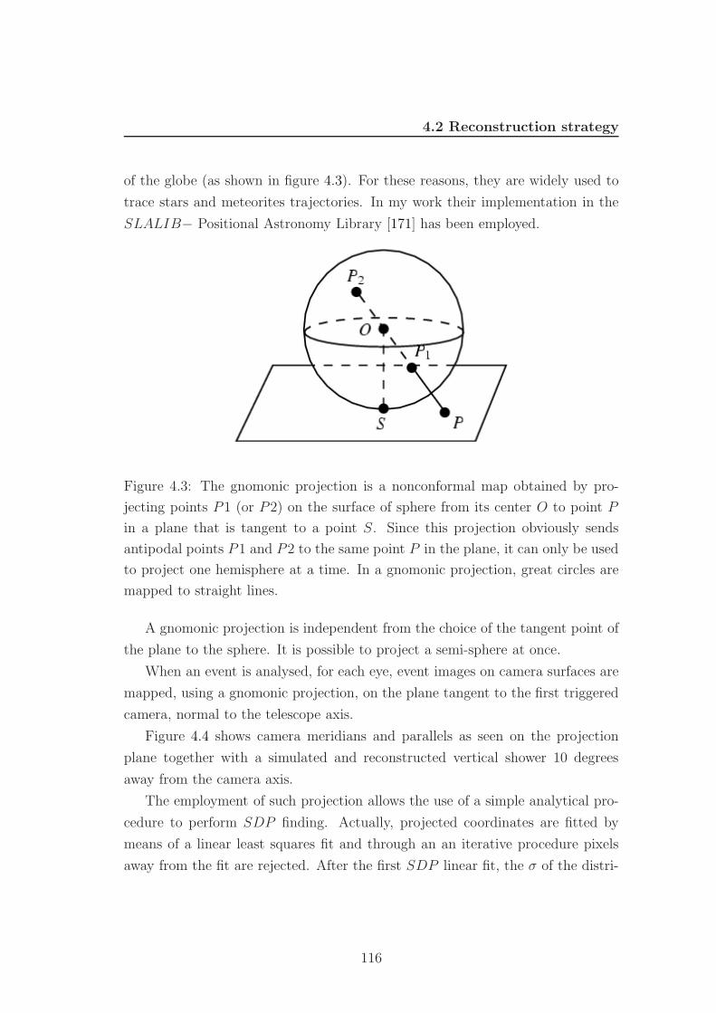
4.2 Reconstruction strategy
of the globe (as shown in figure 4.3). For these reasons, they are widely used to
trace stars and meteorites trajectories. In my work their implementation in the
SLALIB− Positional Astronomy Library [171] has been employed.
Figure 4.3: The gnomonic projection is a nonconformal map obtained by pro-
jecting points P1 (or P2) on the surface of sphere from its center O to point P
in a plane that is tangent to a point S. Since this projection obviously sends
antipodal points P1 and P2 to the same point P in the plane, it can only be used
to project one hemisphere at a time. In a gnomonic projection, great circles are
mapped to straight lines.
A gnomonic projection is independent from the choice of the tangent point of
the plane to the sphere. It is possible to project a semi-sphere at once.
When an event is analysed, for each eye, event images on camera surfaces are
mapped, using a gnomonic projection, on the plane tangent to the first triggered
camera, normal to the telescope axis.
Figure 4.4 shows camera meridians and parallels as seen on the projection
plane together with a simulated and reconstructed vertical shower 10 degrees
away from the camera axis.
The employment of such projection allows the use of a simple analytical pro-
cedure to perform SDP finding. Actually, projected coordinates are fitted by
means of a linear least squares fit and through an an iterative procedure pixels
away from the fit are rejected. After the first SDP linear fit, the σ of the distri-
116
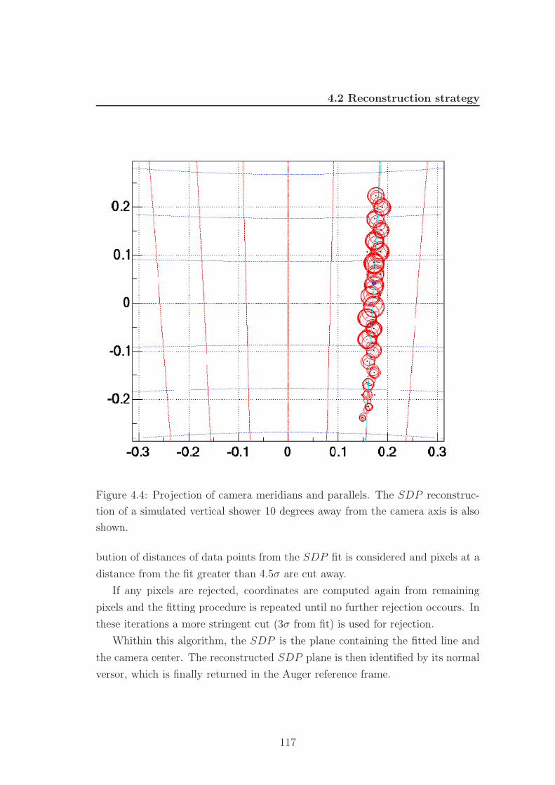
4.2 Reconstruction strategy
Figure 4.4: Projection of camera meridians and parallels. The SDP reconstruc-
tion of a simulated vertical shower 10 degrees away from the camera axis is also
shown.
bution of distances of data points from the SDP fit is considered and pixels at a
distance from the fit greater than 4.5σ are cut away.
If any pixels are rejected, coordinates are computed again from remaining
pixels and the fitting procedure is repeated until no further rejection occours. In
these iterations a more stringent cut (3σ from fit) is used for rejection.
Whithin this algorithm, the SDP is the plane containing the fitted line and
the camera center. The reconstructed SDP plane is then identified by its normal
versor, which is finally returned in the Auger reference frame.
117

4.3 Performances of the method
4.3 Performances of the method
In order to check the performances of the method I used simulated showers of
known energy and geometry. Showers were generated using the FDSim - FDTrig-
gerSim1 [172] chain, version v2r2 updated from cvs on july 2, 2004 after some
corrections. The analysis was performed with the Auger Offline snap-20040625
updated from cvs on july 8, 2004 after some bug fixing.
Since FDTriggerSim simulated showers are generated using the calibraton
constants of bay 4 in the Engeneering Array and these constants were not present
in the database used by the Offline framework2, I set the event time of generated
events at january 2000 (when the FD was not operating) and added a special
entry in my local copy of the database at that date, with the constants used in
the simulation. With this choice I was able to analyze simulated showers with
appropriate calibration constants.
A sets of 1000 Gaisser Hillas parametrized vertical showers produced by proton
primaries was simulated at various distances in the middle of the field of view
of bay 4 at Los Leones. In both simulation and reconstruction processes I used
a clean atmosphere as distributed by the Auger simulation task group, in which
the aerosol horizontal atenuation length is 25 km and the vertical scale height is
2 km.
The energies of simulated showers were fixed at 1018 1019 and 1020 eV, the
distances from the shower core and the FD were selected between 5 and 40 km,
according to the shower energy. All events were analysed with the default Offline
reconstruction and with my approach, using the two definition of coordinates
described in sec. 4.2.2 for both approaches.
1The possibility to perform event simulation within the Offline framework has been imple-mented only during this year. Up to now, event simulation containing the detector responsehas been made by using FDSim - FDTRiggerSim package for the FD and SDSim for the SD.
2In order to take into of the time-varying telescope calibration constants, they are storedin a MySQL database
118
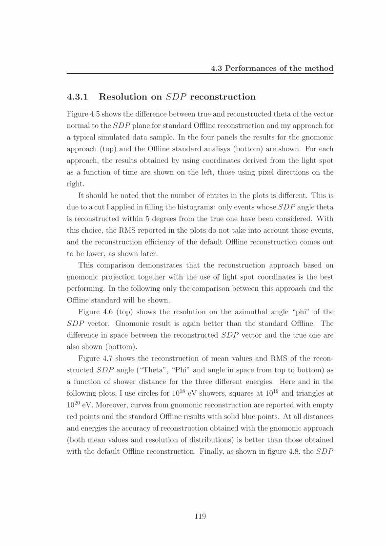
4.3 Performances of the method
4.3.1 Resolution on SDP reconstruction
Figure 4.5 shows the difference between true and reconstructed theta of the vector
normal to the SDP plane for standard Offline reconstruction and my approach for
a typical simulated data sample. In the four panels the results for the gnomonic
approach (top) and the Offline standard analisys (bottom) are shown. For each
approach, the results obtained by using coordinates derived from the light spot
as a function of time are shown on the left, those using pixel directions on the
right.
It should be noted that the number of entries in the plots is different. This is
due to a cut I applied in filling the histograms: only events whose SDP angle theta
is reconstructed within 5 degrees from the true one have been considered. With
this choice, the RMS reported in the plots do not take into account those events,
and the reconstruction efficiency of the default Offline reconstruction comes out
to be lower, as shown later.
This comparison demonstrates that the reconstruction approach based on
gnomonic projection together with the use of light spot coordinates is the best
performing. In the following only the comparison between this approach and the
Offline standard will be shown.
Figure 4.6 (top) shows the resolution on the azimuthal angle “phi” of the
SDP vector. Gnomonic result is again better than the standard Offline. The
difference in space between the reconstructed SDP vector and the true one are
also shown (bottom).
Figure 4.7 shows the reconstruction of mean values and RMS of the recon-
structed SDP angle (“Theta”, “Phi” and angle in space from top to bottom) as
a function of shower distance for the three different energies. Here and in the
following plots, I use circles for 1018 eV showers, squares at 1019 and triangles at
1020 eV. Moreover, curves from gnomonic reconstruction are reported with empty
red points and the standard Offline results with solid blue points. At all distances
and energies the accuracy of reconstruction obtained with the gnomonic approach
(both mean values and resolution of distributions) is better than those obtained
with the default Offline reconstruction. Finally, as shown in figure 4.8, the SDP
119
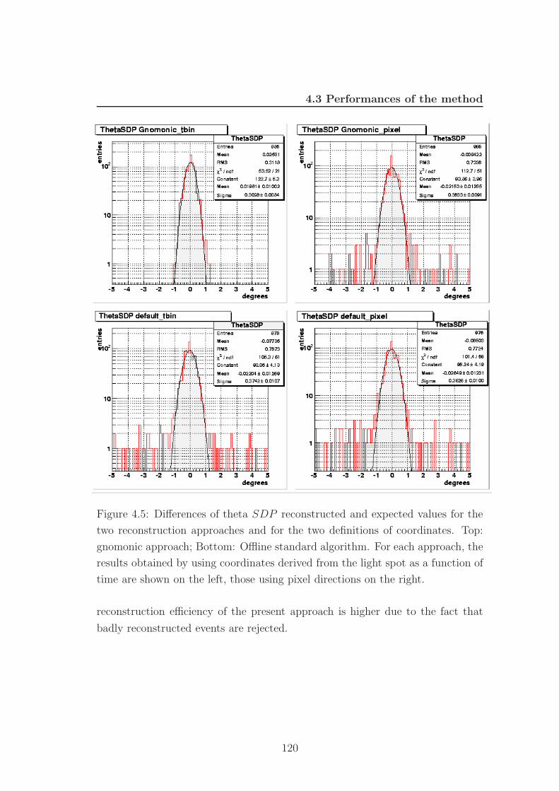
4.3 Performances of the method
Figure 4.5: Differences of theta SDP reconstructed and expected values for the
two reconstruction approaches and for the two definitions of coordinates. Top:
gnomonic approach; Bottom: Offline standard algorithm. For each approach, the
results obtained by using coordinates derived from the light spot as a function of
time are shown on the left, those using pixel directions on the right.
reconstruction efficiency of the present approach is higher due to the fact that
badly reconstructed events are rejected.
120
4.3 Performances of the method
Figure 4.6: Reconstruction results for phi SDP for the gnomonic approach (left)
and for the Offline standard (right) for azimuthal angle (top) and for the SDP
angle in space (bottom).
121
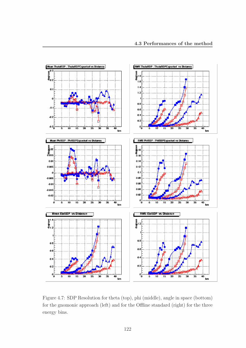
4.3 Performances of the method
Figure 4.7: SDP Resolution for theta (top), phi (middle), angle in space (bottom)
for the gnomonic approach (left) and for the Offline standard (right) for the three
energy bins.
122
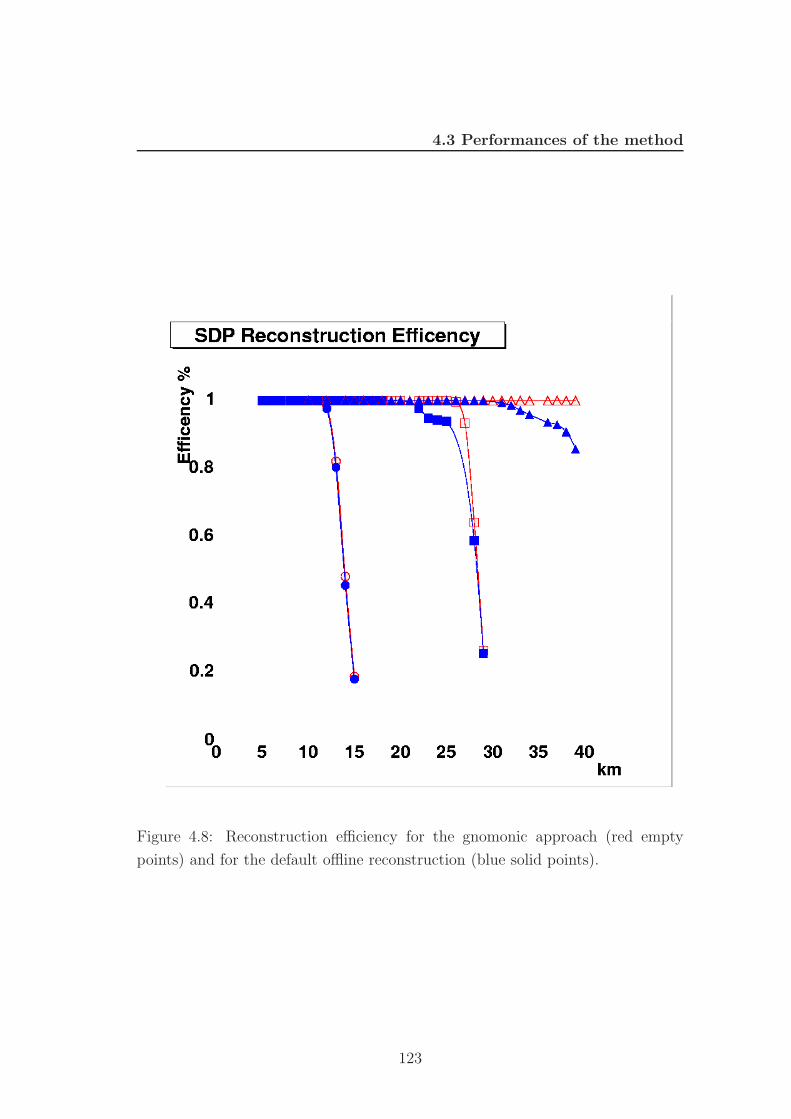
4.3 Performances of the method
Figure 4.8: Reconstruction efficiency for the gnomonic approach (red empty
points) and for the default offline reconstruction (blue solid points).
123

4.4 Effect of improved SDP resolution on shower reconstruction
4.4 Effect of improved SDP resolution on shower
reconstruction
The reconstruction of the shower detector plane is only the first step in the FD
event reconstruction procedure, and has an impact on the way next steps are
performed. For this reason I compare the reconstruction of shower axis, core
position, Xmax and Nmax for the two SDP reconstruction approaches.
Figure 4.9 shows the comparison of reconstructed shower geometry for the
two SDP approaches. It is clear that the achieved performances are very similar
and not sensitive to the SDP reconstruction accuracy, being dominated by the
errors on the time fit procedure. A test on real laser shots (see sec.5.2) shows that
core reconstruction on real events is better performed if the gnomonic approach
is used. Moreover the more accurate pixel selection procedure has an impor-
tant drawback as shown in figure 4.10 where the final geometrical reconstruction
efficiency is shown for both SDP reconstruction approaches for the three consid-
ered energies. Gnomonic reconstruction efficiency is higher, expecially for 1020
eV showers at distances greater than 30 km, where the time fit of the standard
offline reconstruction stream often fails to converge.
In addiction, one finds that the reconstruction of other physical shower proper-
ties benefit from the SDP reconstruction strategy. Figure 4.11 shows an example
of the reconstruction performances in the determination of Xmax and Nmax. The
Xmax accuracy obtained by using the gnomonic SDP reconstruction approach
is 20 g/cm2 less than that one obained with the default reconstruction. This
improvement is very important for mass composition studies. In fact, the most
traditional method developed so far make use of the depth of the shower maxi-
mum and derives an observed mean mass composition as a function of the primary
energy (elongation rate, see section 1.4.8). Furthermore, shower profiles produced
by iron and proton primaries have an average difference on the maximum shower
depth of about 100 g/cm2. Then it is needed to achieve the better accuracy on
Xmax determination.
Figure 4.12 shows the evolution of mean values and RMS of Nmax and Xmax
as a function of distance for the two approaches.
124
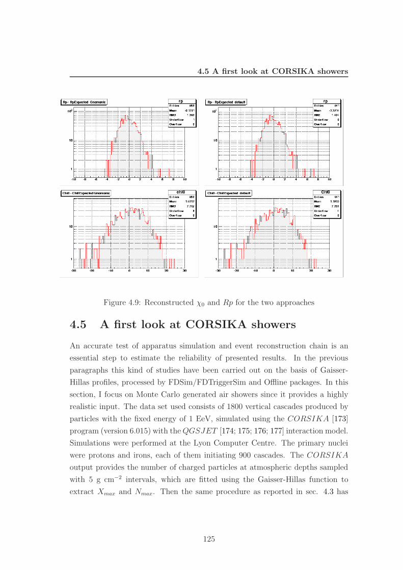
4.5 A first look at CORSIKA showers
Figure 4.9: Reconstructed χ0 and Rp for the two approaches
4.5 A first look at CORSIKA showers
An accurate test of apparatus simulation and event reconstruction chain is an
essential step to estimate the reliability of presented results. In the previous
paragraphs this kind of studies have been carried out on the basis of Gaisser-
Hillas profiles, processed by FDSim/FDTriggerSim and Offline packages. In this
section, I focus on Monte Carlo generated air showers since it provides a highly
realistic input. The data set used consists of 1800 vertical cascades produced by
particles with the fixed energy of 1 EeV, simulated using the CORSIKA [173]
program (version 6.015) with the QGSJET [174; 175; 176; 177] interaction model.
Simulations were performed at the Lyon Computer Centre. The primary nuclei
were protons and irons, each of them initiating 900 cascades. The CORSIKA
output provides the number of charged particles at atmospheric depths sampled
with 5 g cm−2 intervals, which are fitted using the Gaisser-Hillas function to
extract Xmax and Nmax. Then the same procedure as reported in sec. 4.3 has
125
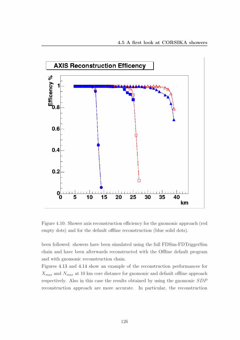
4.5 A first look at CORSIKA showers
Figure 4.10: Shower axis reconstruction efficiency for the gnomonic approach (red
empty dots) and for the default offline reconstruction (blue solid dots).
been followed: showers have been simulated using the full FDSim-FDTriggerSim
chain and have been afterwards reconstructed with the Offline default program
and with gnomonic reconstruction chain.
Figures 4.13 and 4.14 show an example of the reconstruction performances for
Xmax and Nmax at 10 km core distance for gnomonic and default offline approach
respectively. Also in this case the results obtained by using the gnomonic SDP
reconstruction approach are more accurate. In particular, the reconstruction
126
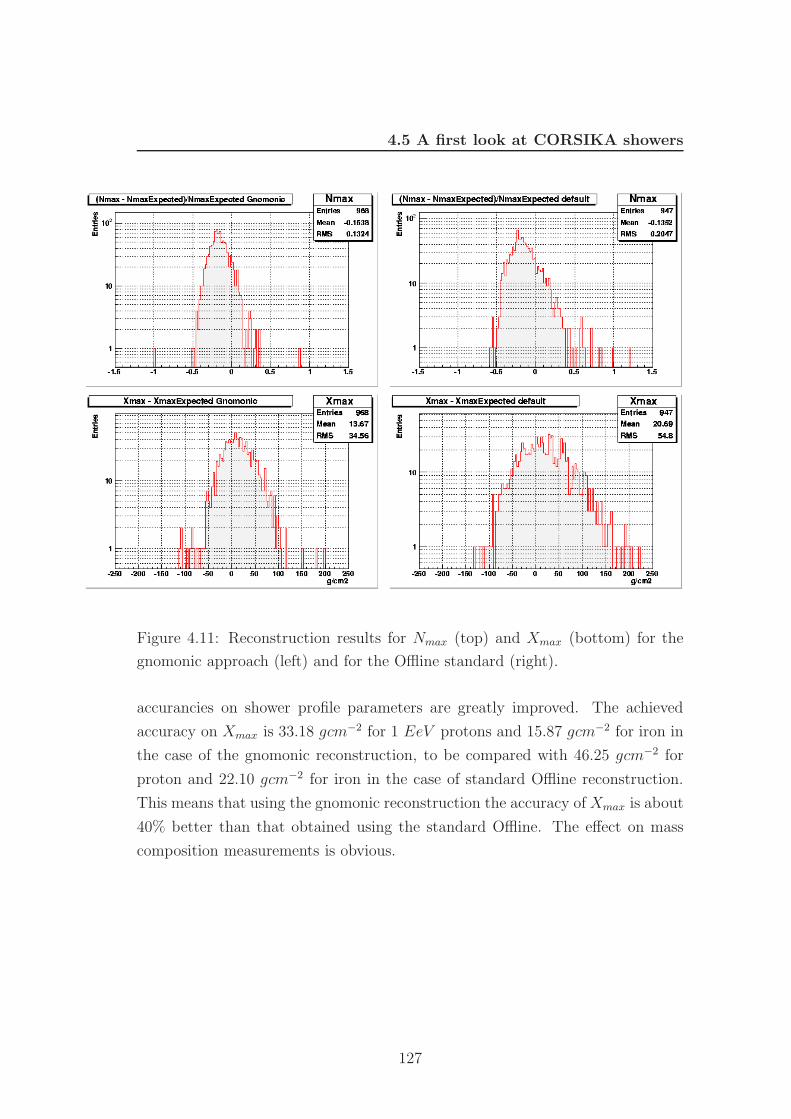
4.5 A first look at CORSIKA showers
Figure 4.11: Reconstruction results for Nmax (top) and Xmax (bottom) for the
gnomonic approach (left) and for the Offline standard (right).
accurancies on shower profile parameters are greatly improved. The achieved
accuracy on Xmax is 33.18 gcm−2 for 1 EeV protons and 15.87 gcm−2 for iron in
the case of the gnomonic reconstruction, to be compared with 46.25 gcm−2 for
proton and 22.10 gcm−2 for iron in the case of standard Offline reconstruction.
This means that using the gnomonic reconstruction the accuracy of Xmax is about
40% better than that obtained using the standard Offline. The effect on mass
composition measurements is obvious.
127
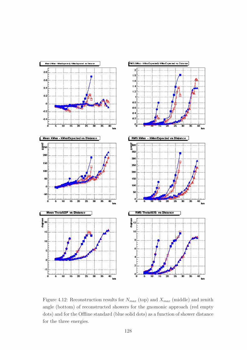
4.5 A first look at CORSIKA showers
Figure 4.12: Reconstruction results for Nmax (top) and Xmax (middle) and zenith
angle (bottom) of reconstructed showers for the gnomonic approach (red empty
dots) and for the Offline standard (blue solid dots) as a function of shower distance
for the three energies.
128
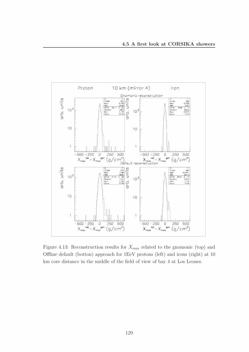
4.5 A first look at CORSIKA showers
Figure 4.13: Reconstruction results for Xmax related to the gnomonic (top) and
Offline default (botton) approach for 1EeV protons (left) and irons (right) at 10
km core distance in the middle of the field of view of bay 4 at Los Leones.
129
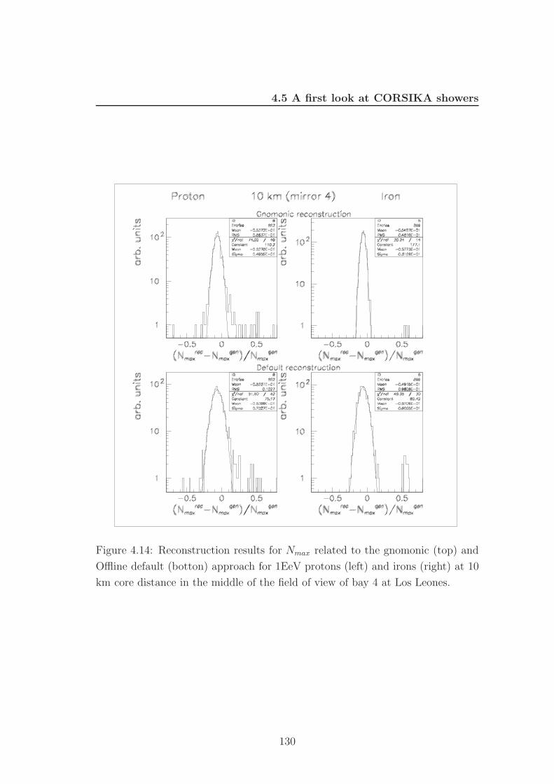
4.5 A first look at CORSIKA showers
Figure 4.14: Reconstruction results for Nmax related to the gnomonic (top) and
Offline default (botton) approach for 1EeV protons (left) and irons (right) at 10
km core distance in the middle of the field of view of bay 4 at Los Leones.
130
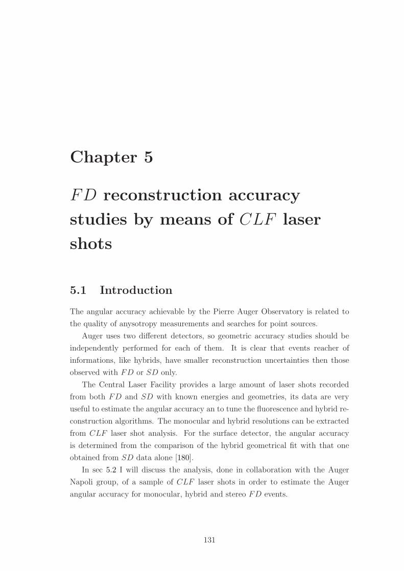
Chapter 5
FD reconstruction accuracy
studies by means of CLF laser
shots
5.1 Introduction
The angular accuracy achievable by the Pierre Auger Observatory is related to
the quality of anysotropy measurements and searches for point sources.
Auger uses two different detectors, so geometric accuracy studies should be
independently performed for each of them. It is clear that events reacher of
informations, like hybrids, have smaller reconstruction uncertainties then those
observed with FD or SD only.
The Central Laser Facility provides a large amount of laser shots recorded
from both FD and SD with known energies and geometries, its data are very
useful to estimate the angular accuracy an to tune the fluorescence and hybrid re-
construction algorithms. The monocular and hybrid resolutions can be extracted
from CLF laser shot analysis. For the surface detector, the angular accuracy
is determined from the comparison of the hybrid geometrical fit with that one
obtained from SD data alone [180].
In sec 5.2 I will discuss the analysis, done in collaboration with the Auger
Napoli group, of a sample of CLF laser shots in order to estimate the Auger
angular accuracy for monocular, hybrid and stereo FD events.
131
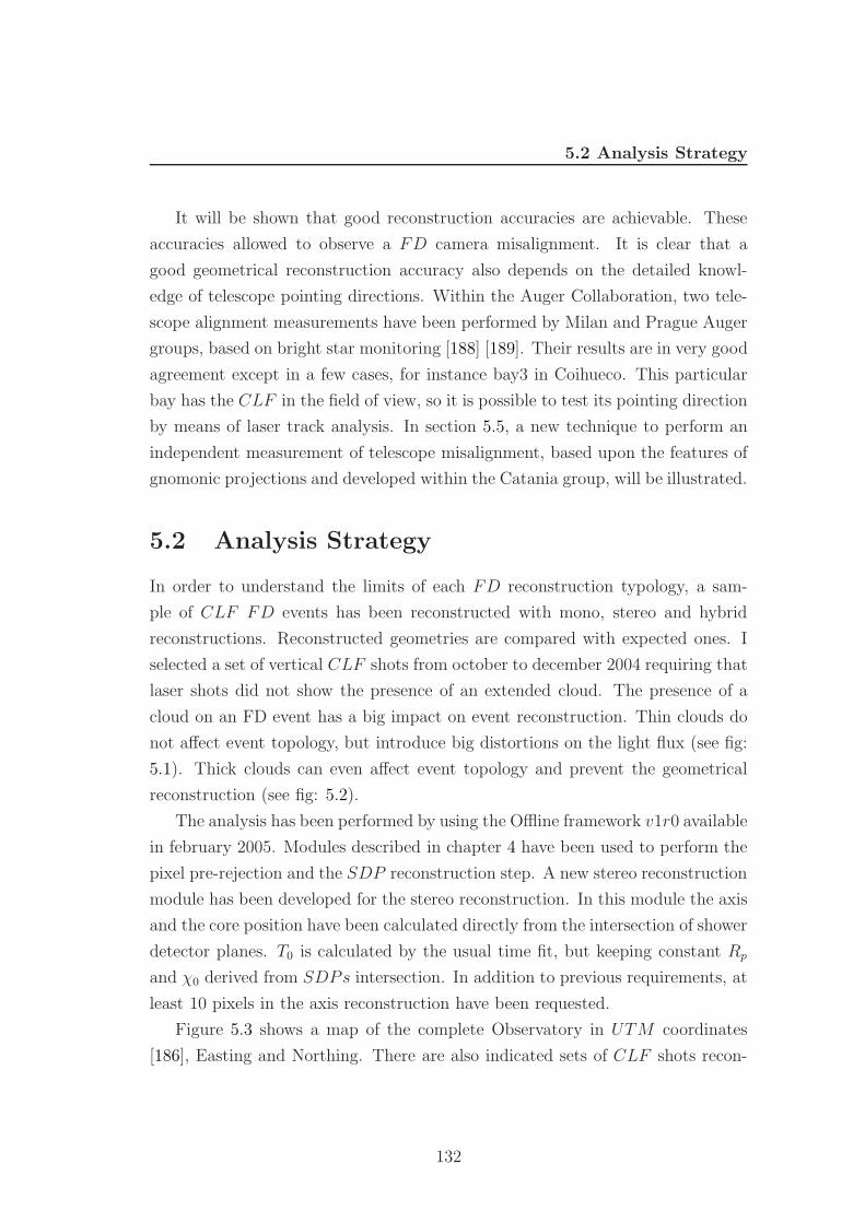
5.2 Analysis Strategy
It will be shown that good reconstruction accuracies are achievable. These
accuracies allowed to observe a FD camera misalignment. It is clear that a
good geometrical reconstruction accuracy also depends on the detailed knowl-
edge of telescope pointing directions. Within the Auger Collaboration, two tele-
scope alignment measurements have been performed by Milan and Prague Auger
groups, based on bright star monitoring [188] [189]. Their results are in very good
agreement except in a few cases, for instance bay3 in Coihueco. This particular
bay has the CLF in the field of view, so it is possible to test its pointing direction
by means of laser track analysis. In section 5.5, a new technique to perform an
independent measurement of telescope misalignment, based upon the features of
gnomonic projections and developed within the Catania group, will be illustrated.
5.2 Analysis Strategy
In order to understand the limits of each FD reconstruction typology, a sam-
ple of CLF FD events has been reconstructed with mono, stereo and hybrid
reconstructions. Reconstructed geometries are compared with expected ones. I
selected a set of vertical CLF shots from october to december 2004 requiring that
laser shots did not show the presence of an extended cloud. The presence of a
cloud on an FD event has a big impact on event reconstruction. Thin clouds do
not affect event topology, but introduce big distortions on the light flux (see fig:
5.1). Thick clouds can even affect event topology and prevent the geometrical
reconstruction (see fig: 5.2).
The analysis has been performed by using the Offline framework v1r0 available
in february 2005. Modules described in chapter 4 have been used to perform the
pixel pre-rejection and the SDP reconstruction step. A new stereo reconstruction
module has been developed for the stereo reconstruction. In this module the axis
and the core position have been calculated directly from the intersection of shower
detector planes. T0 is calculated by the usual time fit, but keeping constant Rp
and χ0 derived from SDPs intersection. In addition to previous requirements, at
least 10 pixels in the axis reconstruction have been requested.
Figure 5.3 shows a map of the complete Observatory in UTM coordinates
[186], Easting and Northing. There are also indicated sets of CLF shots recon-
132
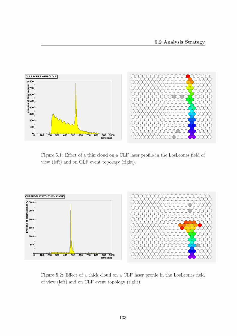
5.2 Analysis Strategy
h1Entries 1630Mean 411.4RMS 130.2
Time [ns]0 100 200 300 400 500 600 700 800 900 1000
ph
oto
ns
at d
iap
hra
gm
/m^2
0
100
200
300
400
500
600
700
800
h1Entries 1630Mean 411.4RMS 130.2CLF PROFILE WITH CLOUD
Figure 5.1: Effect of a thin cloud on a CLF laser profile in the LosLeones field of
view (left) and on CLF event topology (right).
h1Entries 1575Mean 437.2RMS 89.5
Time [ns]0 100 200 300 400 500 600 700 800 900 1000
ph
oto
ns
at d
iap
hra
gm
/m^2
0
500
1000
1500
2000
2500
3000
h1Entries 1575Mean 437.2RMS 89.5CLF PROFILE WITH THICK CLOUD
Figure 5.2: Effect of a thick cloud on a CLF laser profile in the LosLeones field
of view (left) and on CLF event topology (right).
133
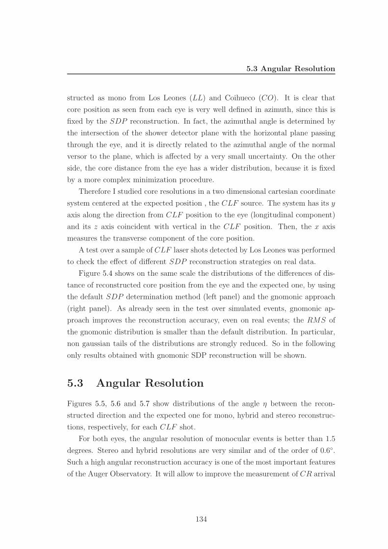
5.3 Angular Resolution
structed as mono from Los Leones (LL) and Coihueco (CO). It is clear that
core position as seen from each eye is very well defined in azimuth, since this is
fixed by the SDP reconstruction. In fact, the azimuthal angle is determined by
the intersection of the shower detector plane with the horizontal plane passing
through the eye, and it is directly related to the azimuthal angle of the normal
versor to the plane, which is affected by a very small uncertainty. On the other
side, the core distance from the eye has a wider distribution, because it is fixed
by a more complex minimization procedure.
Therefore I studied core resolutions in a two dimensional cartesian coordinate
system centered at the expected position , the CLF source. The system has its y
axis along the direction from CLF position to the eye (longitudinal component)
and its z axis coincident with vertical in the CLF position. Then, the x axis
measures the transverse component of the core position.
A test over a sample of CLF laser shots detected by Los Leones was performed
to check the effect of different SDP reconstruction strategies on real data.
Figure 5.4 shows on the same scale the distributions of the differences of dis-
tance of reconstructed core position from the eye and the expected one, by using
the default SDP determination method (left panel) and the gnomonic approach
(right panel). As already seen in the test over simulated events, gnomonic ap-
proach improves the reconstruction accuracy, even on real events; the RMS of
the gnomonic distribution is smaller than the default distribution. In particular,
non gaussian tails of the distributions are strongly reduced. So in the following
only results obtained with gnomonic SDP reconstruction will be shown.
5.3 Angular Resolution
Figures 5.5, 5.6 and 5.7 show distributions of the angle η between the recon-
structed direction and the expected one for mono, hybrid and stereo reconstruc-
tions, respectively, for each CLF shot.
For both eyes, the angular resolution of monocular events is better than 1.5
degrees. Stereo and hybrid resolutions are very similar and of the order of 0.6.
Such a high angular reconstruction accuracy is one of the most important features
of the Auger Observatory. It will allow to improve the measurement of CR arrival
134
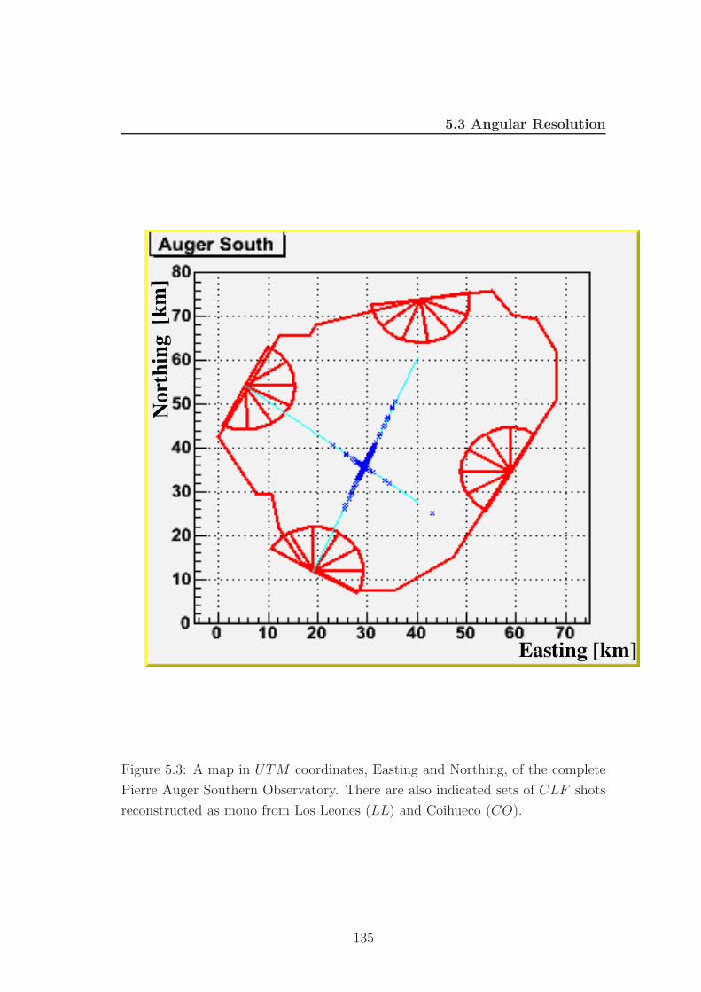
5.3 Angular Resolution
Easting [km]
Nor
thin
g [k
m]
Figure 5.3: A map in UTM coordinates, Easting and Northing, of the complete
Pierre Auger Southern Observatory. There are also indicated sets of CLF shots
reconstructed as mono from Los Leones (LL) and Coihueco (CO).
135
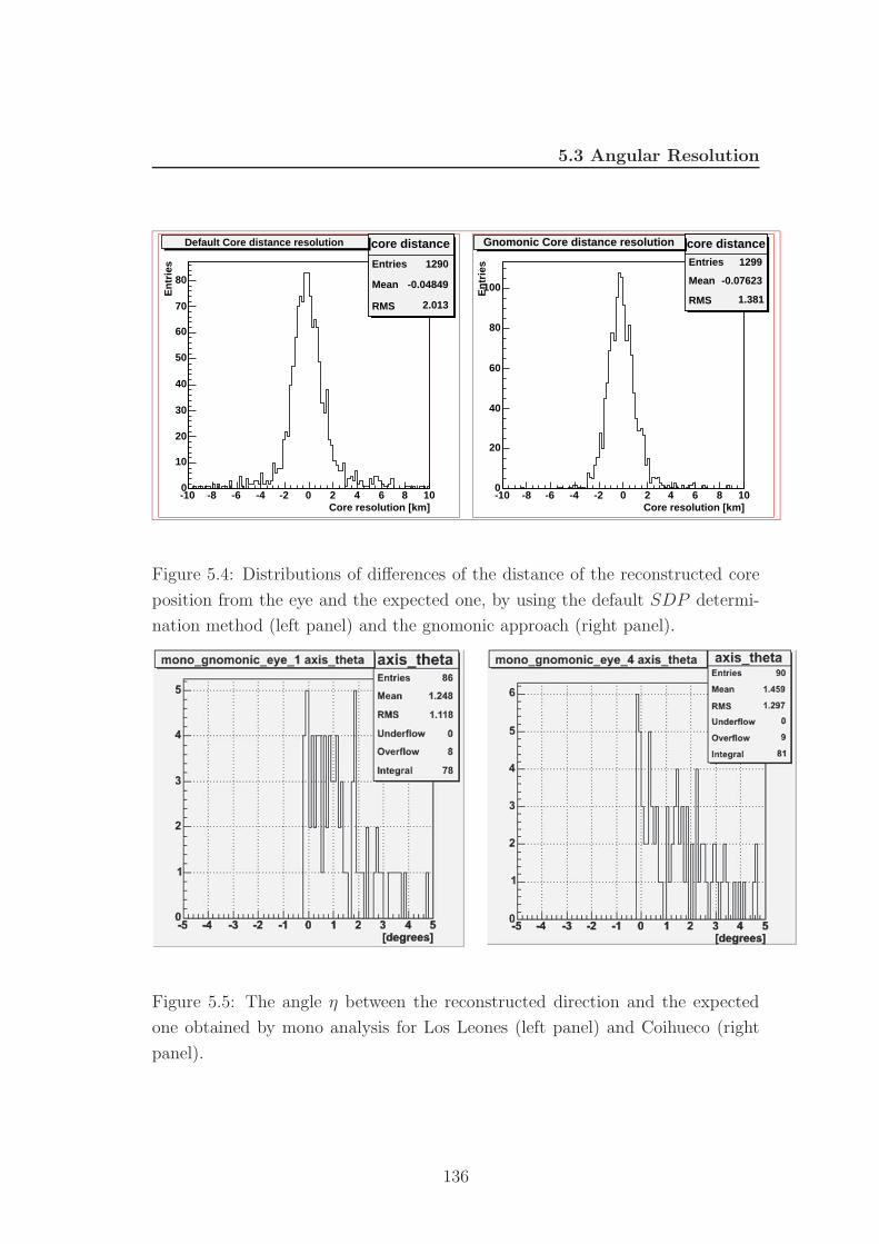
5.3 Angular Resolution
core distance
Entries 1290
Mean -0.04849
RMS 2.013
Core resolution [km]-10 -8 -6 -4 -2 0 2 4 6 8 10
En
trie
s
0
10
20
30
40
50
60
70
80
core distance
Entries 1290
Mean -0.04849
RMS 2.013
Default Core distance resolution core distanceEntries 1299
Mean -0.07623
RMS 1.381
Core resolution [km]-10 -8 -6 -4 -2 0 2 4 6 8 10
En
trie
s0
20
40
60
80
100
core distanceEntries 1299
Mean -0.07623
RMS 1.381
Gnomonic Core distance resolution
Figure 5.4: Distributions of differences of the distance of the reconstructed core
position from the eye and the expected one, by using the default SDP determi-
nation method (left panel) and the gnomonic approach (right panel).
Figure 5.5: The angle η between the reconstructed direction and the expected
one obtained by mono analysis for Los Leones (left panel) and Coihueco (right
panel).
136
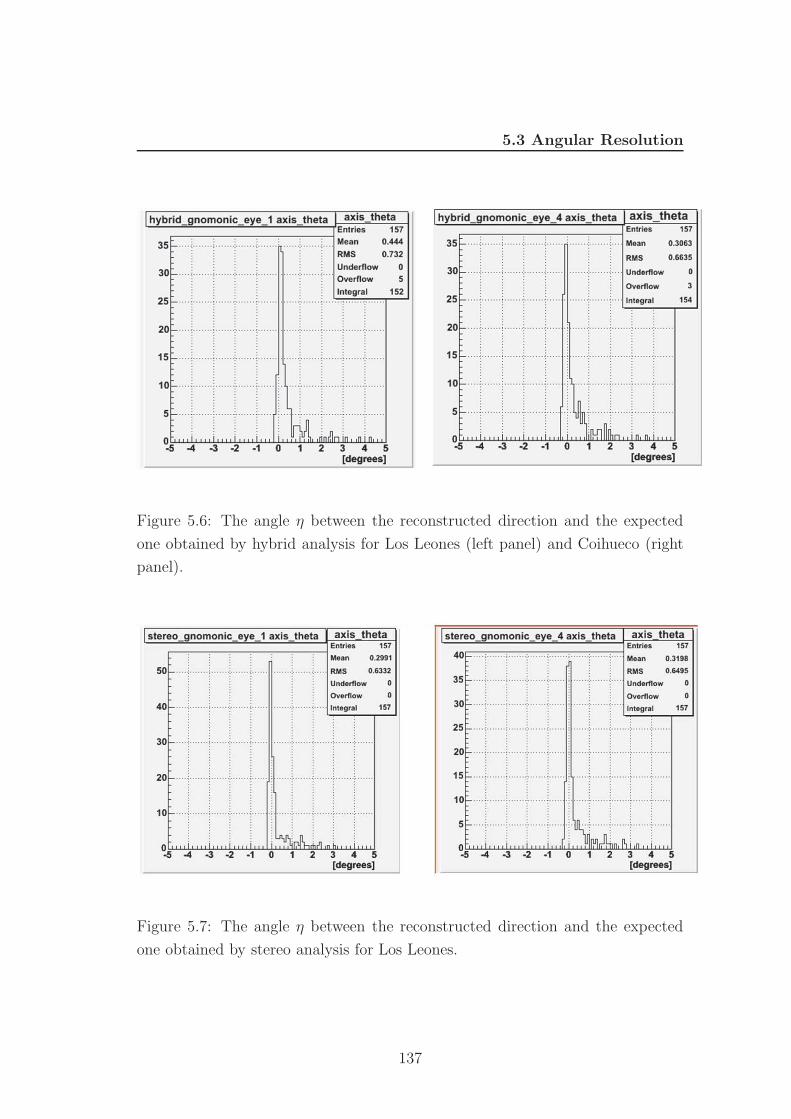
5.3 Angular Resolution
Figure 5.6: The angle η between the reconstructed direction and the expected
one obtained by hybrid analysis for Los Leones (left panel) and Coihueco (right
panel).
Figure 5.7: The angle η between the reconstructed direction and the expected
one obtained by stereo analysis for Los Leones.
137
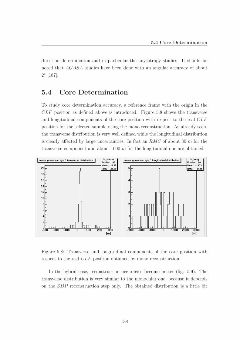
5.4 Core Determination
direction determination and in particular the anysotropy studies. It should be
noted that AGASA studies have been done with an angular accuracy of about
2 [187].
5.4 Core Determination
To study core determination accuracy, a reference frame with the origin in the
CLF position as defined above is introduced. Figure 5.8 shows the transverse
and longitudinal components of the core position with respect to the real CLF
position for the selected sample using the mono reconstruction. As already seen,
the transverse distribution is very well defined while the longitudinal distribution
is clearly affected by large uncertainties. In fact an RMS of about 30 m for the
transverse component and about 1000 m for the longitudinal one are obtained.
h_transvEntries 86Mean 22.35RMS 26.09
[m]-300 -200 -100 0 100 200 3000
2
4
6
8
10
12
14
16
18
20
h_transvEntries 86Mean 22.35RMS 26.09
mono_gnomonic_eye_1 transverse distribution h_longEntries 86Mean -180.4RMS 1028
[m]-3000 -2000 -1000 0 1000 2000 3000
0
1
2
3
4
5
h_longEntries 86Mean -180.4RMS 1028
mono_gnomonic_eye_1 longitudinal distribution
Figure 5.8: Transverse and longitudinal components of the core position with
respect to the real CLF position obtained by mono reconstruction.
In the hybrid case, reconstruction accuracies become better (fig. 5.9). The
transverse distribution is very similar to the monocular one, because it depends
on the SDP reconstruction step only. The obtained distribution is a little bit
138
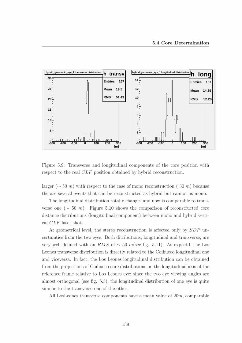
5.4 Core Determination
h_transvEntries 157
Mean 19.5
RMS 51.43
[m]-300 -200 -100 0 100 200 3000
5
10
15
20
25
30h_transvEntries 157
Mean 19.5
RMS 51.43
hybrid_gnomonic_eye_1 transverse distribution h_longEntries 157
Mean -14.39
RMS 52.28
[m]-300 -200 -100 0 100 200 3000
2
4
6
8
10
12
14
h_longEntries 157
Mean -14.39
RMS 52.28
hybrid_gnomonic_eye_1 longitudinal distribution
Figure 5.9: Transverse and longitudinal components of the core position with
respect to the real CLF position obtained by hybrid reconstruction.
larger (∼ 50 m) with respect to the case of mono reconstruction ( 30 m) because
the are several events that can be reconstructed as hybrid but cannot as mono.
The longitudinal distribution totally changes and now is comparable to trans-
verse one (∼ 50 m). Figure 5.10 shows the comparison of reconstructed core
distance distributions (longitudinal component) between mono and hybrid verti-
cal CLF laser shots.
At geometrical level, the stereo reconstruction is affected only by SDP un-
certainties from the two eyes. Both ditributions, longitudinal and transverse, are
very well defined with an RMS of ∼ 50 m(see fig. 5.11). As expectd, the Los
Leones transverse distribution is directly related to the Coihueco longitudinal one
and viceversa. In fact, the Los Leones longitudinal distribution can be obtained
from the projections of Coihueco core distributions on the longitudinal axis of the
reference frame relative to Los Leones eye; since the two eye viewing angles are
almost orthogonal (see fig. 5.3), the longitudinal distribution of one eye is quite
similar to the transverse one of the other.
All LosLeones transverse components have a mean value of 20m, comparable
139
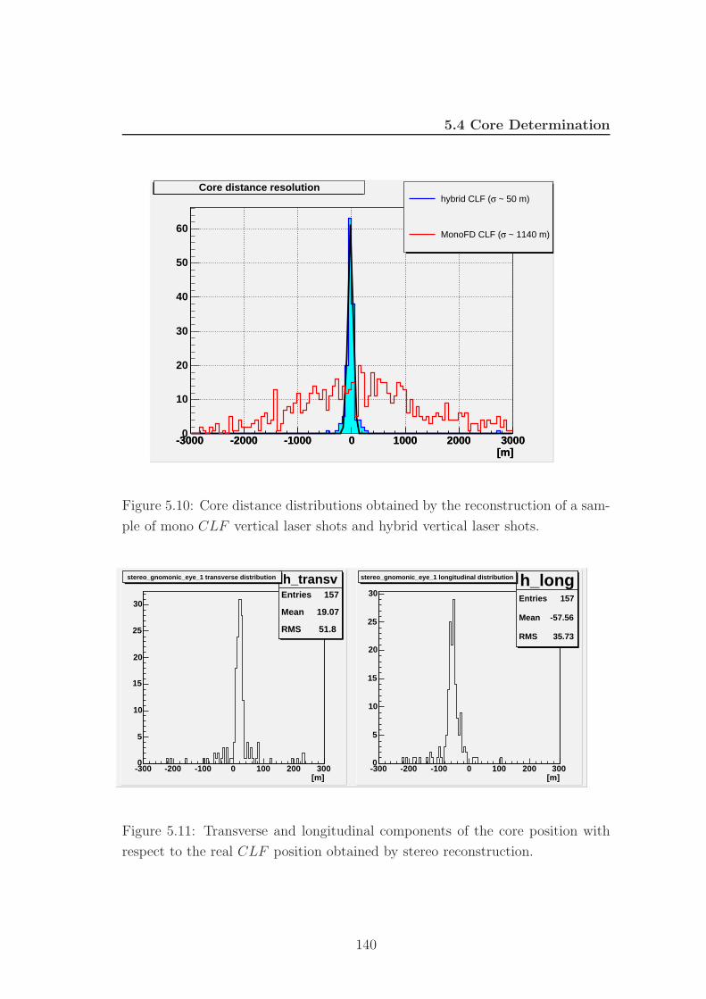
5.4 Core Determination
[m]-3000 -2000 -1000 0 1000 2000 3000
distanceEntries 147Mean -1.588RMS 243
[m]-3000 -2000 -1000 0 1000 2000 30000
10
20
30
40
50
60
distanceEntries 147Mean -1.588RMS 243
~ 50 m)σhybrid CLF (
~ 1140 m)σMonoFD CLF (
Core distance resolution
Figure 5.10: Core distance distributions obtained by the reconstruction of a sam-
ple of mono CLF vertical laser shots and hybrid vertical laser shots.
h_transvEntries 187
Mean 19
RMS 51.69
[m]-300 -200 -100 0 100 200 3000
5
10
15
20
25
30
h_transvEntries 157
Mean 19.07
RMS 51.8
stereo_gnomonic_eye_1 transverse distribution h_longEntries 185
Mean -57.46
RMS 35.79
[m]-300 -200 -100 0 100 200 3000
5
10
15
20
25
30h_longEntries 157
Mean -57.56
RMS 35.73
stereo_gnomonic_eye_1 longitudinal distribution
Figure 5.11: Transverse and longitudinal components of the core position with
respect to the real CLF position obtained by stereo reconstruction.
140
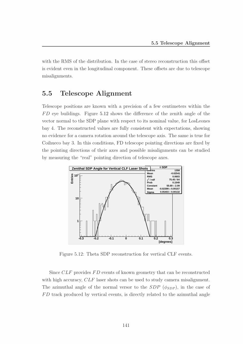
5.5 Telescope Alignment
with the RMS of the distribution. In the case of stereo reconstruction this offset
is evident even in the longitudinal component. These offsets are due to telescope
misalignments.
5.5 Telescope Alignment
Telescope positions are known with a precision of a few centimeters within the
FD eye buildings. Figure 5.12 shows the difference of the zenith angle of the
vector normal to the SDP plane with respect to its nominal value, for LosLeones
bay 4. The reconstructed values are fully consistent with expectations, showing
no evidence for a camera rotation around the telescope axis. The same is true for
Coihueco bay 3. In this conditions, FD telescope pointing directions are fixed by
the pointing directions of their axes and possible misalignments can be studied
by measuring the “real” pointing direction of telescope axes.
SDPθEntries 1358Mean -0.02541RMS 0.0603
/ ndf 2χ 75.45 / 64Prob 0.1549Constant 2.09± 55.69 Mean 0.00157± -0.02399 Sigma 0.00132± 0.05403
[degrees]-0.3 -0.2 -0.1 0 0.1 0.2 0.3
En
trie
s
1
10
210
SDPθEntries 1358Mean -0.02541RMS 0.0603
/ ndf 2χ 75.45 / 64Prob 0.1549Constant 2.09± 55.69 Mean 0.00157± -0.02399 Sigma 0.00132± 0.05403
Zenithal SDP Angle for Vertical CLF Laser Shots
Figure 5.12: Theta SDP reconstruction for vertical CLF events.
Since CLF provides FD events of known geometry that can be reconstructed
with high accuracy, CLF laser shots can be used to study camera misalignment.
The azimuthal angle of the normal versor to the SDP (φSDP ), in the case of
FD track produced by vertical events, is directly related to the azimuthal angle
141
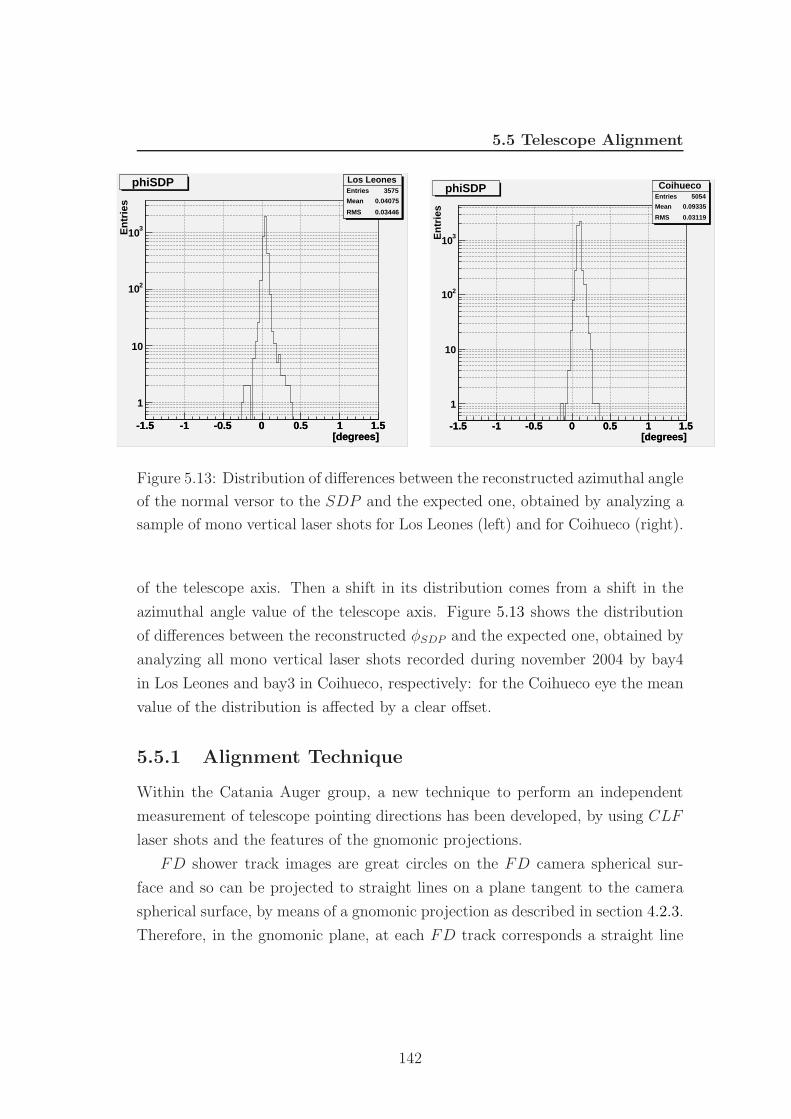
5.5 Telescope Alignment
[degrees]-1.5 -1 -0.5 0 0.5 1 1.5
Los LeonesEntries 3575
Mean 0.04075
RMS 0.03446
[degrees]-1.5 -1 -0.5 0 0.5 1 1.5
En
trie
s
1
10
210
310
Los LeonesEntries 3575
Mean 0.04075
RMS 0.03446
phiSDP
[degrees]-1.5 -1 -0.5 0 0.5 1 1.5
CoihuecoEntries 5054
Mean 0.09335
RMS 0.03119
[degrees]-1.5 -1 -0.5 0 0.5 1 1.5
En
trie
s
1
10
210
310
CoihuecoEntries 5054
Mean 0.09335
RMS 0.03119
phiSDP
Figure 5.13: Distribution of differences between the reconstructed azimuthal angle
of the normal versor to the SDP and the expected one, obtained by analyzing a
sample of mono vertical laser shots for Los Leones (left) and for Coihueco (right).
of the telescope axis. Then a shift in its distribution comes from a shift in the
azimuthal angle value of the telescope axis. Figure 5.13 shows the distribution
of differences between the reconstructed φSDP and the expected one, obtained by
analyzing all mono vertical laser shots recorded during november 2004 by bay4
in Los Leones and bay3 in Coihueco, respectively: for the Coihueco eye the mean
value of the distribution is affected by a clear offset.
5.5.1 Alignment Technique
Within the Catania Auger group, a new technique to perform an independent
measurement of telescope pointing directions has been developed, by using CLF
laser shots and the features of the gnomonic projections.
FD shower track images are great circles on the FD camera spherical sur-
face and so can be projected to straight lines on a plane tangent to the camera
spherical surface, by means of a gnomonic projection as described in section 4.2.3.
Therefore, in the gnomonic plane, at each FD track corresponds a straight line
142
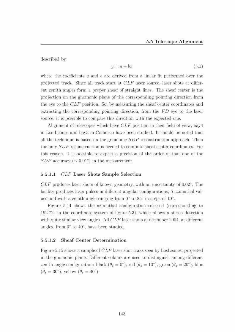
5.5 Telescope Alignment
described by
y = a + bx (5.1)
where the coefficients a and b are derived from a linear fit performed over the
projected track. Since all track start at CLF laser source, laser shots at differ-
ent zenith angles form a proper sheaf of straight lines. The sheaf center is the
projection on the gnomonic plane of the corresponding pointing direction from
the eye to the CLF position. So, by measuring the sheaf center coordinates and
extracting the corresponding pointing direction, from the FD eye to the laser
source, it is possible to compare this direction with the expected one.
Alignment of telescopes which have CLF position in their field of view, bay4
in Los Leones and bay3 in Coihueco have been studied. It should be noted that
all the technique is based on the gnomonic SDP reconstruction approach. Then
the only SDP reconstruction is needed to compute sheaf center coordinates. For
this reason, it is possible to expect a precision of the order of that one of the
SDP accuracy (∼ 0.01) in the measurement.
5.5.1.1 CLF Laser Shots Sample Selection
CLF produces laser shots of known geometry, with an uncertainty of 0.02. The
facility produces laser pulses in different angular configurations, 5 azimuthal val-
ues and with a zenith angle ranging from 0 to 85 in steps of 10.
Figure 5.14 shows the azimuthal configuration selected (corresponding to
192.72 in the coordinate system of figure 5.3), which allows a stereo detection
with quite similar view angles. All CLF laser shots of december 2004, at different
angles, from 0 to 40, have been studied.
5.5.1.2 Sheaf Center Determination
Figure 5.15 shows a sample of CLF laser shot traks seen by LosLeones, projected
in the gnomonic plane. Different colours are used to distinguish among different
zenith angle configuration: black (θz = 0), red (θz = 10), green (θz = 20), blue
(θz = 30), yellow (θz = 40).
143
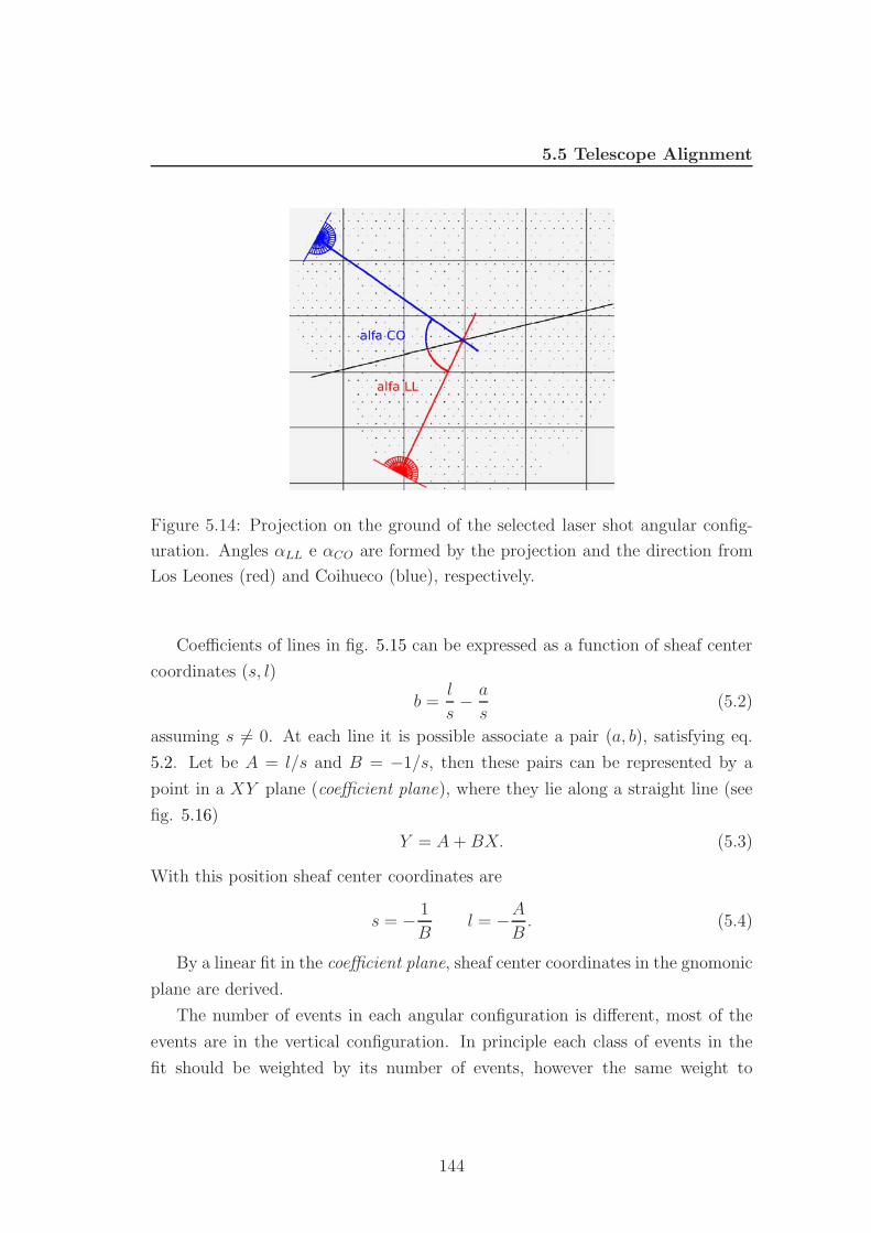
5.5 Telescope Alignment
Figure 5.14: Projection on the ground of the selected laser shot angular config-
uration. Angles αLL e αCO are formed by the projection and the direction from
Los Leones (red) and Coihueco (blue), respectively.
Coefficients of lines in fig. 5.15 can be expressed as a function of sheaf center
coordinates (s, l)
b =l
s− a
s(5.2)
assuming s = 0. At each line it is possible associate a pair (a, b), satisfying eq.
5.2. Let be A = l/s and B = −1/s, then these pairs can be represented by a
point in a XY plane (coefficient plane), where they lie along a straight line (see
fig. 5.16)
Y = A + BX. (5.3)
With this position sheaf center coordinates are
s = − 1
Bl = −A
B. (5.4)
By a linear fit in the coefficient plane, sheaf center coordinates in the gnomonic
plane are derived.
The number of events in each angular configuration is different, most of the
events are in the vertical configuration. In principle each class of events in the
fit should be weighted by its number of events, however the same weight to
144
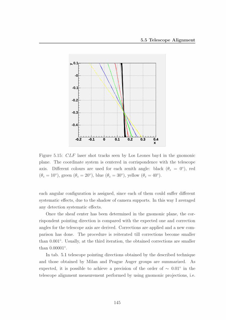
5.5 Telescope Alignment
x-0.2 -0.1 0 0.1 0.2 0.3 0.4
x-0.2 -0.1 0 0.1 0.2 0.3 0.4
y
-0.4
-0.3
-0.2
-0.1
-0
0.1
Figure 5.15: CLF laser shot tracks seen by Los Leones bay4 in the gnomonic
plane. The coordinate system is centered in corrispondence with the telescope
axis. Different colours are used for each zenith angle: black (θz = 0), red
(θz = 10), green (θz = 20), blue (θz = 30), yellow (θz = 40).
each angular configuration is assigned, since each of them could suffer different
systematic effects, due to the shadow of camera supports. In this way I averaged
any detection systematic effects.
Once the sheaf center has been determined in the gnomonic plane, the cor-
rispondent pointing direction is compared with the expected one and correction
angles for the telescope axis are derived. Corrections are applied and a new com-
parison has done. The procedure is reiterated till corrections become smaller
than 0.001. Usually, at the third iteration, the obtained corrections are smaller
than 0.00001.
In tab. 5.1 telescope pointing directions obtained by the described technique
and those obtained by Milan and Prague Auger groups are summarized. As
expected, it is possible to achieve a precision of the order of ∼ 0.01 in the
telescope alignment measurement performed by using gnomonic projections, i.e.
145
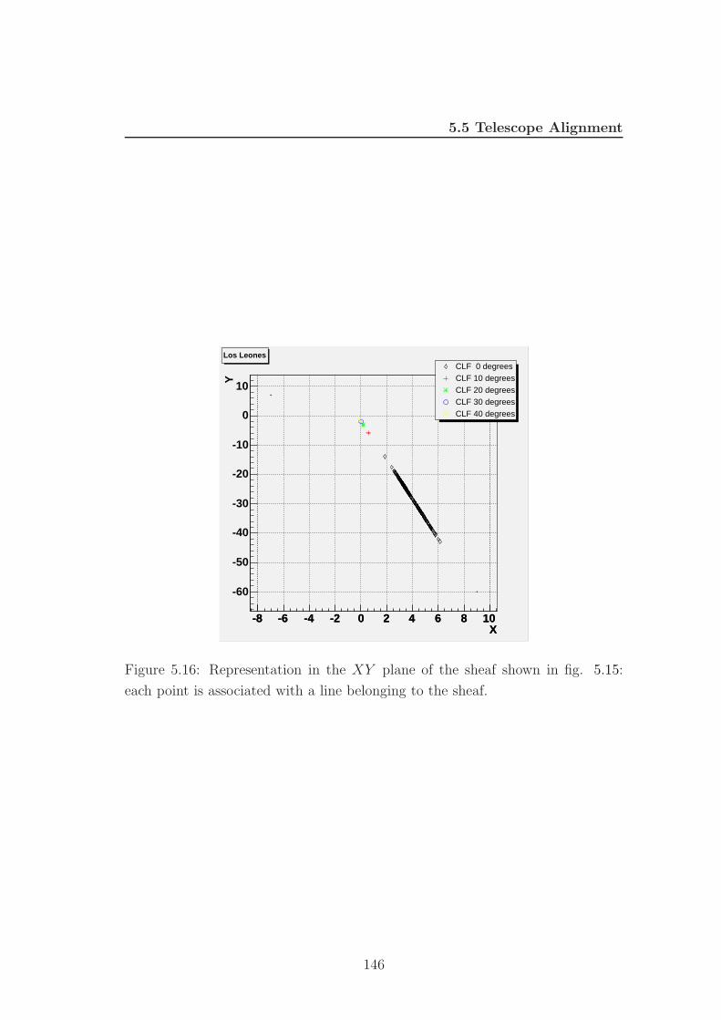
5.5 Telescope Alignment
X-8 -6 -4 -2 0 2 4 6 8 10
X-8 -6 -4 -2 0 2 4 6 8 10
Y
-60
-50
-40
-30
-20
-10
0
10
CLF 0 degreesCLF 10 degreesCLF 20 degreesCLF 30 degreesCLF 40 degrees
Los Leones
Figure 5.16: Representation in the XY plane of the sheaf shown in fig. 5.15:
each point is associated with a line belonging to the sheaf.
146
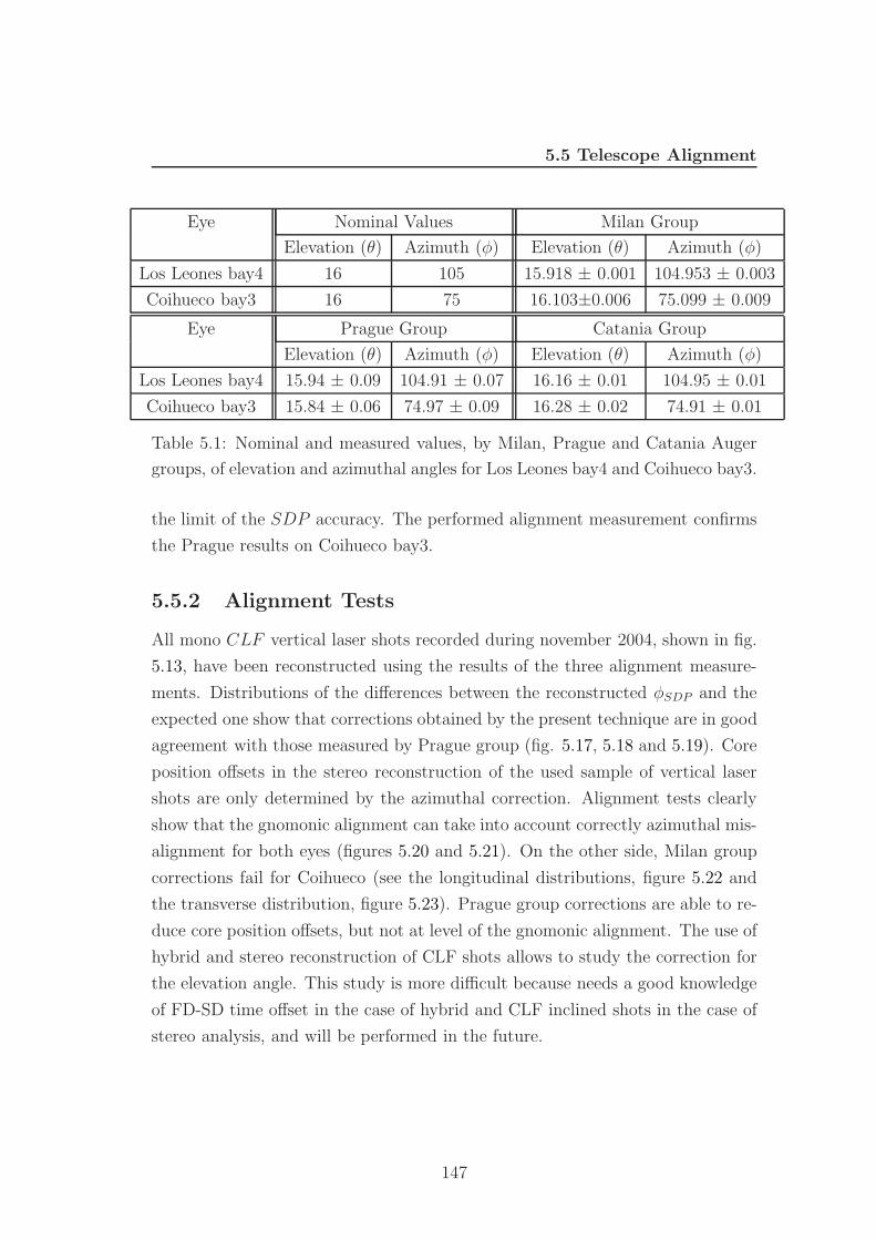
5.5 Telescope Alignment
Eye Nominal Values Milan Group
Elevation (θ) Azimuth (φ) Elevation (θ) Azimuth (φ)
Los Leones bay4 16 105 15.918 ± 0.001 104.953 ± 0.003
Coihueco bay3 16 75 16.103±0.006 75.099 ± 0.009
Eye Prague Group Catania Group
Elevation (θ) Azimuth (φ) Elevation (θ) Azimuth (φ)
Los Leones bay4 15.94 ± 0.09 104.91 ± 0.07 16.16 ± 0.01 104.95 ± 0.01
Coihueco bay3 15.84 ± 0.06 74.97 ± 0.09 16.28 ± 0.02 74.91 ± 0.01
Table 5.1: Nominal and measured values, by Milan, Prague and Catania Auger
groups, of elevation and azimuthal angles for Los Leones bay4 and Coihueco bay3.
the limit of the SDP accuracy. The performed alignment measurement confirms
the Prague results on Coihueco bay3.
5.5.2 Alignment Tests
All mono CLF vertical laser shots recorded during november 2004, shown in fig.
5.13, have been reconstructed using the results of the three alignment measure-
ments. Distributions of the differences between the reconstructed φSDP and the
expected one show that corrections obtained by the present technique are in good
agreement with those measured by Prague group (fig. 5.17, 5.18 and 5.19). Core
position offsets in the stereo reconstruction of the used sample of vertical laser
shots are only determined by the azimuthal correction. Alignment tests clearly
show that the gnomonic alignment can take into account correctly azimuthal mis-
alignment for both eyes (figures 5.20 and 5.21). On the other side, Milan group
corrections fail for Coihueco (see the longitudinal distributions, figure 5.22 and
the transverse distribution, figure 5.23). Prague group corrections are able to re-
duce core position offsets, but not at level of the gnomonic alignment. The use of
hybrid and stereo reconstruction of CLF shots allows to study the correction for
the elevation angle. This study is more difficult because needs a good knowledge
of FD-SD time offset in the case of hybrid and CLF inclined shots in the case of
stereo analysis, and will be performed in the future.
147
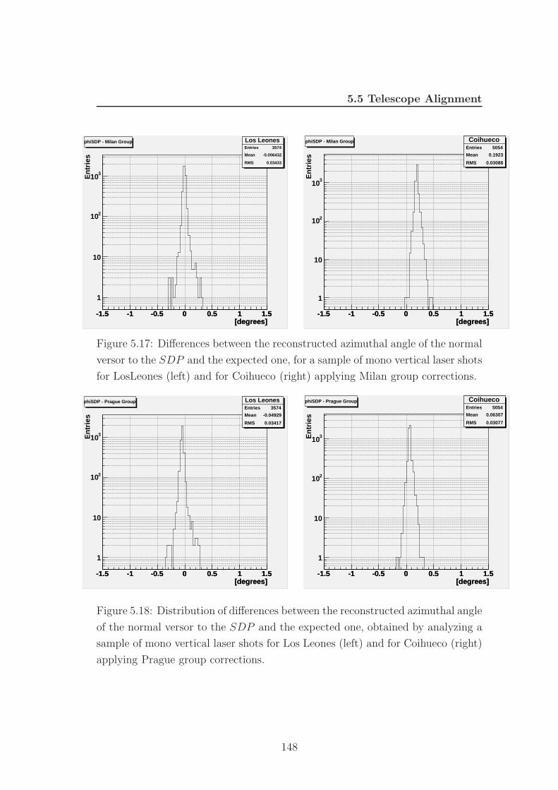
5.5 Telescope Alignment
[degrees]-1.5 -1 -0.5 0 0.5 1 1.5
Los LeonesEntries 3574
Mean -0.006432
RMS 0.03433
[degrees]-1.5 -1 -0.5 0 0.5 1 1.5
En
trie
s
1
10
210
310
Los LeonesEntries 3574
Mean -0.006432
RMS 0.03433
phiSDP - Milan Group
[degrees]-1.5 -1 -0.5 0 0.5 1 1.5
CoihuecoEntries 5054
Mean 0.1923
RMS 0.03088
[degrees]-1.5 -1 -0.5 0 0.5 1 1.5
En
trie
s1
10
210
310
CoihuecoEntries 5054
Mean 0.1923
RMS 0.03088
phiSDP - Milan Group
Figure 5.17: Differences between the reconstructed azimuthal angle of the normal
versor to the SDP and the expected one, for a sample of mono vertical laser shots
for LosLeones (left) and for Coihueco (right) applying Milan group corrections.
[degrees]-1.5 -1 -0.5 0 0.5 1 1.5
Los LeonesEntries 3574
Mean -0.04929
RMS 0.03417
[degrees]-1.5 -1 -0.5 0 0.5 1 1.5
En
trie
s
1
10
210
310
Los LeonesEntries 3574
Mean -0.04929
RMS 0.03417
phiSDP - Prague Group
[degrees]-1.5 -1 -0.5 0 0.5 1 1.5
CoihuecoEntries 5054
Mean 0.06307
RMS 0.03077
[degrees]-1.5 -1 -0.5 0 0.5 1 1.5
En
trie
s
1
10
210
310
CoihuecoEntries 5054
Mean 0.06307
RMS 0.03077
phiSDP - Prague Group
Figure 5.18: Distribution of differences between the reconstructed azimuthal angle
of the normal versor to the SDP and the expected one, obtained by analyzing a
sample of mono vertical laser shots for Los Leones (left) and for Coihueco (right)
applying Prague group corrections.
148
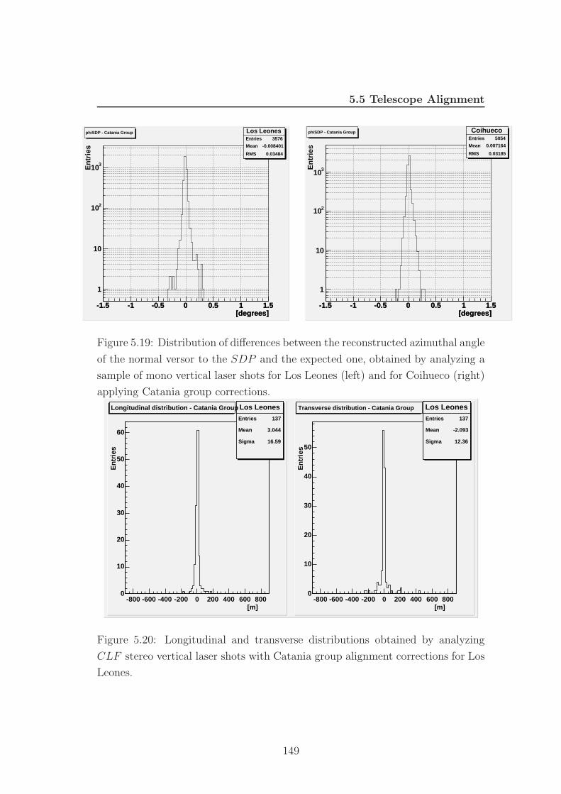
5.5 Telescope Alignment
[degrees]-1.5 -1 -0.5 0 0.5 1 1.5
Los LeonesEntries 3576
Mean -0.008401
RMS 0.03484
[degrees]-1.5 -1 -0.5 0 0.5 1 1.5
En
trie
s
1
10
210
310
Los LeonesEntries 3576
Mean -0.008401
RMS 0.03484
phiSDP - Catania Group
[degrees]-1.5 -1 -0.5 0 0.5 1 1.5
CoihuecoEntries 5054
Mean 0.007164
RMS 0.03185
[degrees]-1.5 -1 -0.5 0 0.5 1 1.5
En
trie
s
1
10
210
310
CoihuecoEntries 5054
Mean 0.007164
RMS 0.03185
phiSDP - Catania Group
Figure 5.19: Distribution of differences between the reconstructed azimuthal angle
of the normal versor to the SDP and the expected one, obtained by analyzing a
sample of mono vertical laser shots for Los Leones (left) and for Coihueco (right)
applying Catania group corrections.
Los LeonesEntries 137
Mean 3.044
Sigma 16.59
[m]-800 -600 -400 -200 0 200 400 600 800
En
trie
s
0
10
20
30
40
50
60
Los LeonesEntries 137
Mean 3.044
Sigma 16.59
Longitudinal distribution - Catania Group Los LeonesEntries 137
Constant 64.7
Mean -2.093
Sigma 12.36
[m]-800 -600 -400 -200 0 200 400 600 800
En
trie
s
0
10
20
30
40
50
Los LeonesEntries 137
Mean -2.093
Sigma 12.36
Transverse distribution - Catania Group
Figure 5.20: Longitudinal and transverse distributions obtained by analyzing
CLF stereo vertical laser shots with Catania group alignment corrections for Los
Leones.
149
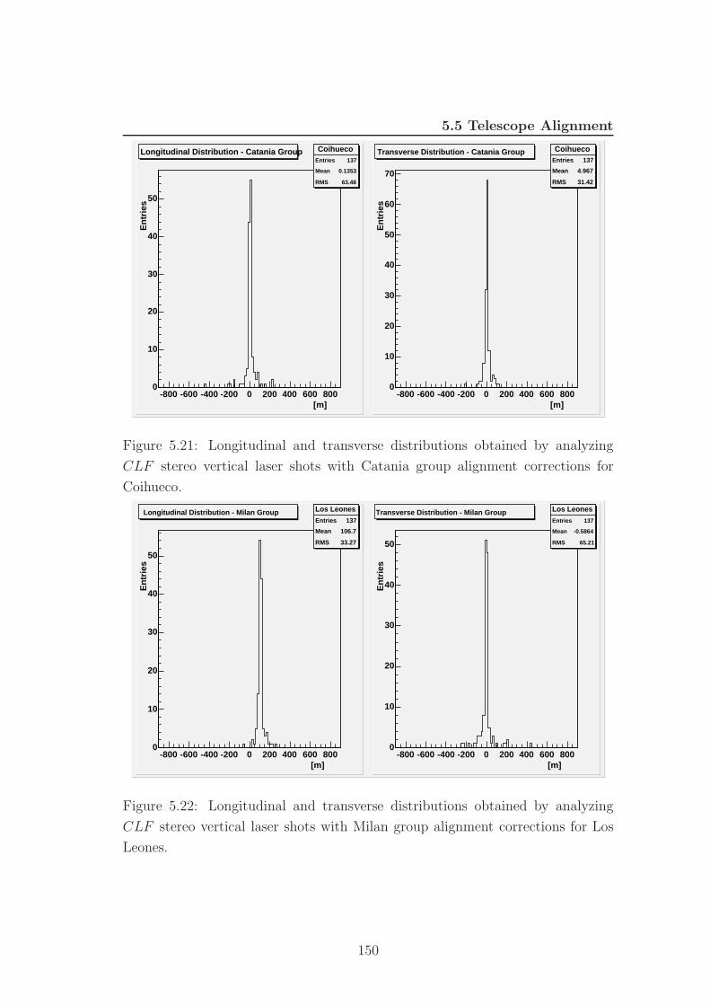
5.5 Telescope Alignment
CoihuecoEntries 137
Mean 0.1353
RMS 63.48
[m]-800 -600 -400 -200 0 200 400 600 800
En
trie
s
0
10
20
30
40
50
CoihuecoEntries 137
Mean 0.1353
RMS 63.48
Longitudinal Distribution - Catania Group CoihuecoEntries 137
Mean 4.967
RMS 31.42
[m]-800 -600 -400 -200 0 200 400 600 800
En
trie
s0
10
20
30
40
50
60
70
CoihuecoEntries 137
Mean 4.967
RMS 31.42
Transverse Distribution - Catania Group
Figure 5.21: Longitudinal and transverse distributions obtained by analyzing
CLF stereo vertical laser shots with Catania group alignment corrections for
Coihueco.
Los Leones
Entries 137
Mean 106.7
RMS 33.27
[m]-800 -600 -400 -200 0 200 400 600 800
En
trie
s
0
10
20
30
40
50
Los Leones
Entries 137
Mean 106.7
RMS 33.27
Longitudinal Distribution - Milan Group Los Leones
Entries 137
Mean -0.5864
RMS 65.21
[m]-800 -600 -400 -200 0 200 400 600 800
En
trie
s
0
10
20
30
40
50
Los Leones
Entries 137
Mean -0.5864
RMS 65.21
Transverse Distribution - Milan Group
Figure 5.22: Longitudinal and transverse distributions obtained by analyzing
CLF stereo vertical laser shots with Milan group alignment corrections for Los
Leones.
150
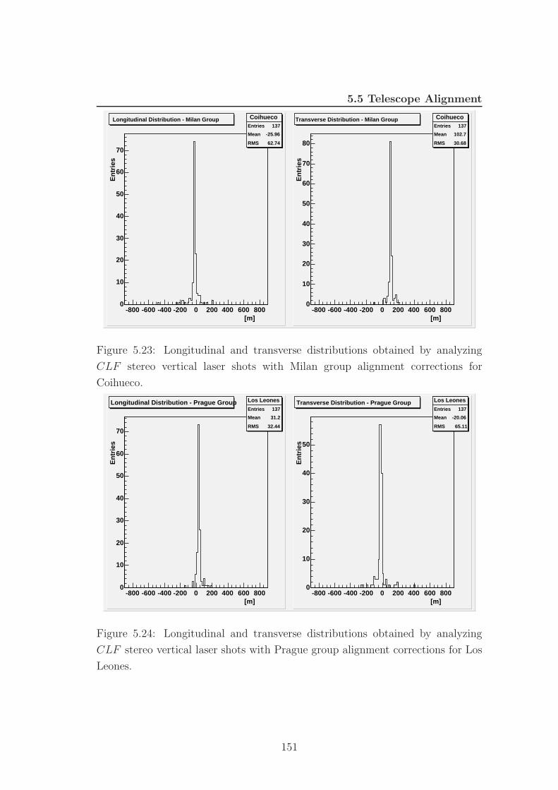
5.5 Telescope Alignment
CoihuecoEntries 137
Mean -25.96
RMS 62.74
[m]-800 -600 -400 -200 0 200 400 600 800
En
trie
s
0
10
20
30
40
50
60
70
CoihuecoEntries 137
Mean -25.96
RMS 62.74
Longitudinal Distribution - Milan Group CoihuecoEntries 137
Mean 102.7
RMS 30.68
[m]-800 -600 -400 -200 0 200 400 600 800
En
trie
s0
10
20
30
40
50
60
70
80
CoihuecoEntries 137
Mean 102.7
RMS 30.68
Transverse Distribution - Milan Group
Figure 5.23: Longitudinal and transverse distributions obtained by analyzing
CLF stereo vertical laser shots with Milan group alignment corrections for
Coihueco.
Los Leones
Entries 137
Mean 31.2
RMS 32.44
[m]-800 -600 -400 -200 0 200 400 600 800
En
trie
s
0
10
20
30
40
50
60
70
Los Leones
Entries 137
Mean 31.2
RMS 32.44
Longitudinal Distribution - Prague Group Los Leones
Entries 137
Mean -20.06
RMS 65.11
[m]-800 -600 -400 -200 0 200 400 600 800
En
trie
s
0
10
20
30
40
50
Los Leones
Entries 137
Mean -20.06
RMS 65.11
Transverse Distribution - Prague Group
Figure 5.24: Longitudinal and transverse distributions obtained by analyzing
CLF stereo vertical laser shots with Prague group alignment corrections for Los
Leones.
151
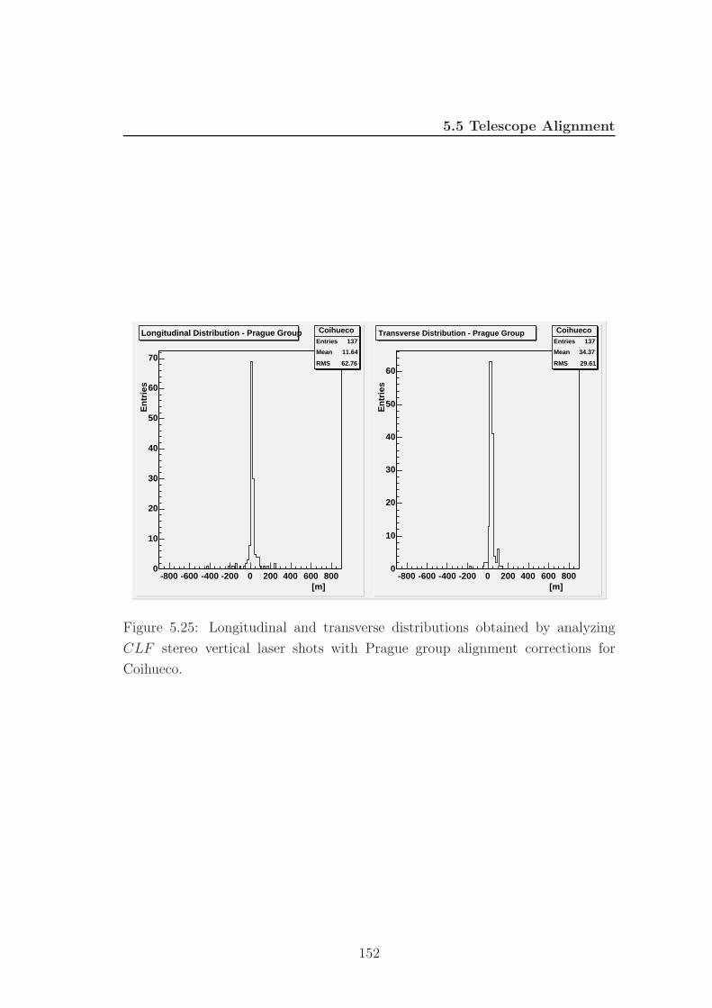
5.5 Telescope Alignment
CoihuecoEntries 137
Mean 11.64
RMS 62.76
[m]-800 -600 -400 -200 0 200 400 600 800
En
trie
s
0
10
20
30
40
50
60
70
CoihuecoEntries 137
Mean 11.64
RMS 62.76
Longitudinal Distribution - Prague Group CoihuecoEntries 137
Mean 34.37
RMS 29.61
[m]-800 -600 -400 -200 0 200 400 600 800
En
trie
s
0
10
20
30
40
50
60
CoihuecoEntries 137
Mean 34.37
RMS 29.61
Transverse Distribution - Prague Group
Figure 5.25: Longitudinal and transverse distributions obtained by analyzing
CLF stereo vertical laser shots with Prague group alignment corrections for
Coihueco.
152
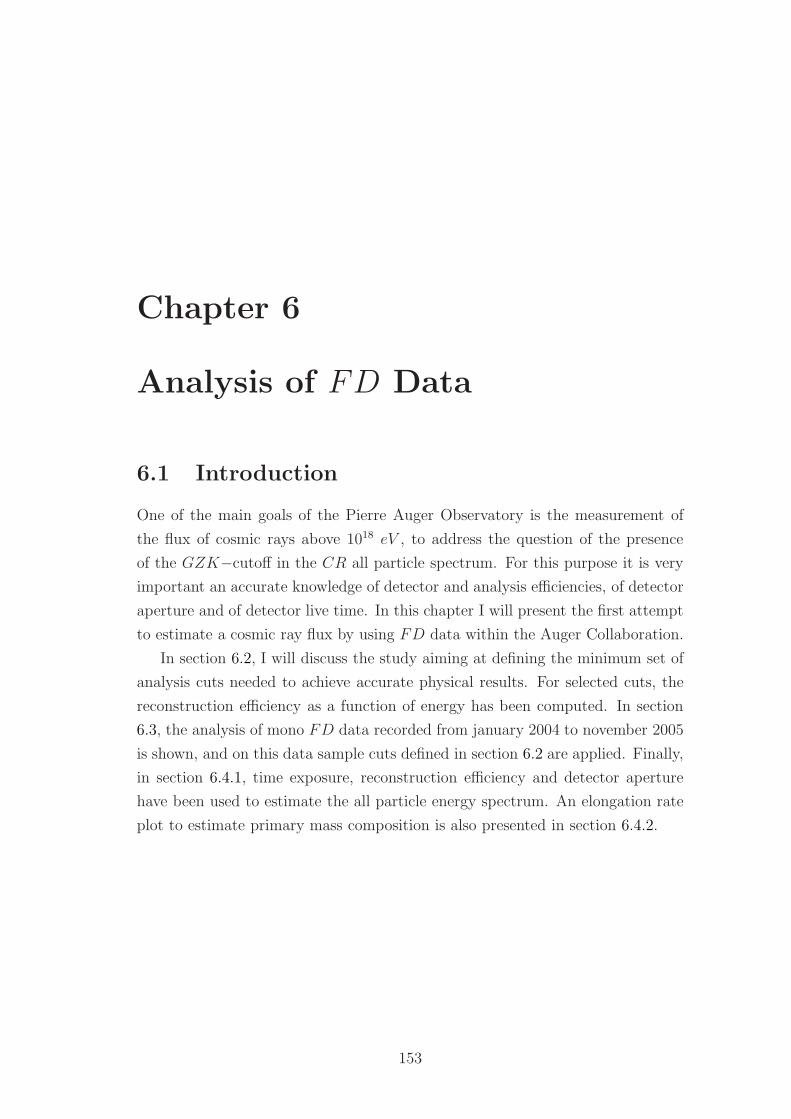
Chapter 6
Analysis of FD Data
6.1 Introduction
One of the main goals of the Pierre Auger Observatory is the measurement of
the flux of cosmic rays above 1018 eV , to address the question of the presence
of the GZK−cutoff in the CR all particle spectrum. For this purpose it is very
important an accurate knowledge of detector and analysis efficiencies, of detector
aperture and of detector live time. In this chapter I will present the first attempt
to estimate a cosmic ray flux by using FD data within the Auger Collaboration.
In section 6.2, I will discuss the study aiming at defining the minimum set of
analysis cuts needed to achieve accurate physical results. For selected cuts, the
reconstruction efficiency as a function of energy has been computed. In section
6.3, the analysis of mono FD data recorded from january 2004 to november 2005
is shown, and on this data sample cuts defined in section 6.2 are applied. Finally,
in section 6.4.1, time exposure, reconstruction efficiency and detector aperture
have been used to estimate the all particle energy spectrum. An elongation rate
plot to estimate primary mass composition is also presented in section 6.4.2.
153
6.2 Reconstruction Accuracy andDefinition Of Analysis Cuts
6.2 Reconstruction Accuracy and
Definition Of Analysis Cuts
The dependence of Observatory’s aperture on numerous parameters has been
studied by means of detailed simulations [178] [179]. FD aperture has been
independently evaluated by two groups within the Auger collaboration with two
different approaches [178; 190]. Aperture studies are based upon the analysis of
large samples of simulated data and their differences will be discussed in section
6.4.1.3. The simulated sample used in [178] is available since march 2005 and it
has been used to estimate the reconstruction efficiency presented in this chapter.
In the following sections I will present the details of the analysis, and I will test
the application of the procedure to a set of real data (sec 6.3).
6.2.1 The Simulated Data Sample
There are important issues emerging from trigger aperture studies, that can be
used into the reconstruction efficiency determination:
1. The FD trigger aperture is almost independent from primary mass compo-
sition. Showers produced by proton and iron primary particles have been
used to test the FD trigger detector with very similar results.
2. The use of two different atmospheric conditions has shown an effect at
trigger level which, as expected, depends on the primary energy. The two
atmosphere have a vertical aerosol optical depth (VAOD) at 3 km above
FD level of 0.03 and 0.06, respectively. At 1018 eV , the trigger aperture for
the cleaner atmosphere is higher than the other one of 15%. The effect is
smaller at higher and lower energies. In fact at lower energies the detector
produces a trigger mainly on near showers, so aerosol effects on fluorescence
light propagation become negligible. At higher energies, the detector always
produces a trigger signal and the effect of atmosphere conditions affects the
energy determination only.
154
6.2 Reconstruction Accuracy andDefinition Of Analysis Cuts
The employed atmospheres are usually referred to as “clean” and “dirty”, be-
cause they have a lower and an higher VAOD with respect to the typical Malargue
atmosphere [181].
Keeping in mind these considerations, the selected data sample used in the
following consists of simulated proton showers produced by using FDSim [172]
with these characteristics:
1. no detailed shower Monte Carlo simulation but a Gaisser-Hillas parametriza-
tion [182];
2. 10000 showers times 8 energy bins at fixed values of Log(E/eV ) = 17, 17.5,
18, 18.5, 19, 19.5, 20, 20.5;
3. zenith angle within 60 degrees, with a cos θd(cos θ) zenith distribution and
uniform azimuth distribution;
4. showers propagated through an atmosphere with a VAOD at 3 km above
the FD level of 0.03, described by a two-parameter Mie model (see sec.
1.4.6.1) with an aerosol horizontal attenuation length LM of 25 km and an
aerosol scale height HM of 2.0 km;
5. shower cores uniformly distributed within the field of view of a single tele-
scope, bay4 of the Los Leones eye and up to distance from the eye that
depends on the energy (6 km at 1017 eV up to 80 km for E > 1019.5 eV );
6.2.2 Definition of Analysis Cuts
In order to define the criteria required to achieve an accurate shower reconstru-
tion, the main shower parameters ( SDP , shower axis, Xmax and shower energy)
have been studied. It was possible to define cuts that allow to reach a good re-
construction accuracy and to evaluated the detector reconstruction efficiency at
different levels.
The analysis has been done using the Offline Framework v1r1, available in
april 2005. Simulated events are reconstructed as monocular events. In the re-
construction module sequence, SDP reconstruction modules described in chapter
155
6.2 Reconstruction Accuracy andDefinition Of Analysis Cuts
4 have been used. In this way I used a pixel pre-rejection and the gnomonic pro-
jections to reconstruct the shower detector plane. In collaboration with L’Aquila
group, I inserted in the Offline a module to reject noise events: the module imple-
ments a Hough filter [184], proposed by L’Aquila group as an on-line filter [185].
The simulation software is not able to produce such events and as expected the
module did not reject any simulated event. On the other side, among real data
there are a lot of these dense noise events (see fig. 6.1) and the implemented
algorithm rejects them very efficiently.
• At geometrical level, one should not directly consider the axis determination
accuracy, but it is also important to study SDP determination. In fact,
in the case of stereo events it is enough to be able to estimate the shower
detector plane for both eyes to get a shower axis reconstruction with a very
small uncertainty.
• To check the quality of the time fit procedure a linear interpolation over
the distribution of pixel timing as a function of pixel elevation angles χi
within the SDP (in the following I will refer to it simply as χi−plot) in
addition to the traditional minimization was performed. The underlying
idea is that, if data do not exhibit a clear curvature (see fig. 3.7), it is not
possible to perform a reliable 3 parameters minimization, In such a case,
data are well fitted by the linear interpolation and the quality of this linear
approximation can be evaluated by its χ2. So high χ2 values correspond to
FD tracks with a clear curvature and a cut can be easily defined.
I studied the reconstruction accuracy of the axis as a function of different
parameters:
1. number of pixels used to calculate the variable under esamination;
2. angular width of the visible part of the recorded shower;
3. event time length;
4. quality of the linear interpolation of the χi−plot.
156
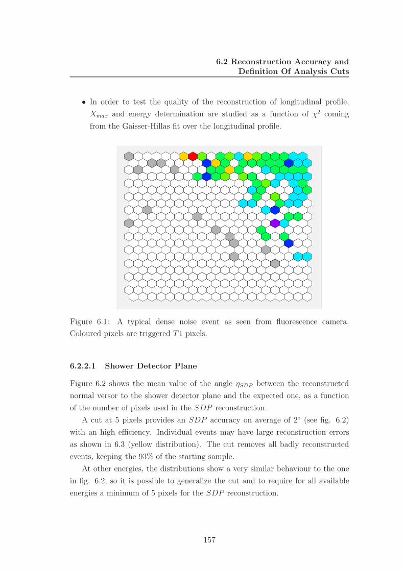
6.2 Reconstruction Accuracy andDefinition Of Analysis Cuts
• In order to test the quality of the reconstruction of longitudinal profile,
Xmax and energy determination are studied as a function of χ2 coming
from the Gaisser-Hillas fit over the longitudinal profile.
Figure 6.1: A typical dense noise event as seen from fluorescence camera.
Coloured pixels are triggered T1 pixels.
6.2.2.1 Shower Detector Plane
Figure 6.2 shows the mean value of the angle ηSDP between the reconstructed
normal versor to the shower detector plane and the expected one, as a function
of the number of pixels used in the SDP reconstruction.
A cut at 5 pixels provides an SDP accuracy on average of 2 (see fig. 6.2)
with an high efficiency. Individual events may have large reconstruction errors
as shown in 6.3 (yellow distribution). The cut removes all badly reconstructed
events, keeping the 93% of the starting sample.
At other energies, the distributions show a very similar behaviour to the one
in fig. 6.2, so it is possible to generalize the cut and to require for all available
energies a minimum of 5 pixels for the SDP reconstruction.
157
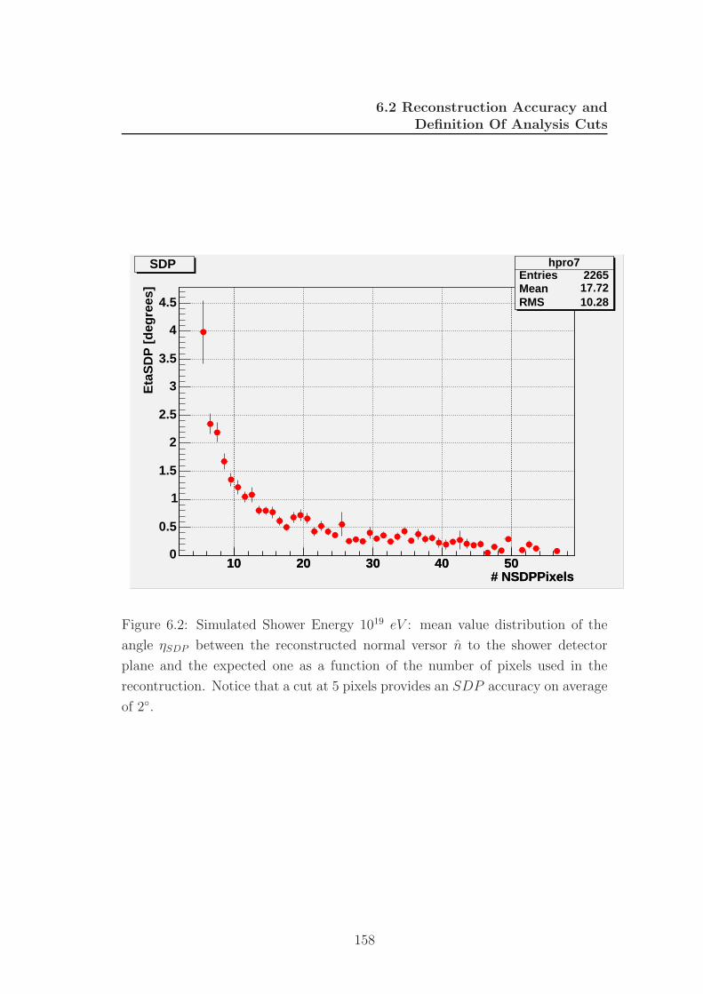
6.2 Reconstruction Accuracy andDefinition Of Analysis Cuts
# NSDPPixels10 20 30 40 50
hpro7Entries 2265Mean 17.72RMS 10.28
# NSDPPixels10 20 30 40 50
Eta
SD
P [
deg
rees
]
0
0.5
1
1.5
2
2.5
3
3.5
4
4.5
hpro7Entries 2265Mean 17.72RMS 10.28
SDP
Figure 6.2: Simulated Shower Energy 1019 eV : mean value distribution of the
angle ηSDP between the reconstructed normal versor n to the shower detector
plane and the expected one as a function of the number of pixels used in the
recontruction. Notice that a cut at 5 pixels provides an SDP accuracy on average
of 2.
158
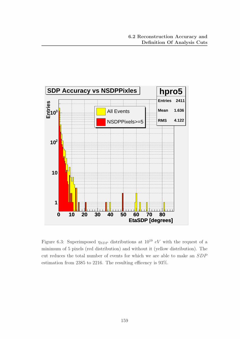
6.2 Reconstruction Accuracy andDefinition Of Analysis Cuts
EtaSDP [degrees] 0 10 20 30 40 50 60 70 80
hpro5Entries 2411
Mean 1.636
RMS 4.122
EtaSDP [degrees] 0 10 20 30 40 50 60 70 80
En
trie
s
1
10
210
310
hpro5Entries 2411
Mean 1.636
RMS 4.122
SDP Accuracy vs NSDPPixles
All Events
NSDPPixels>=5
Figure 6.3: Superimposed ηSDP distributions at 1019 eV with the request of a
minimum of 5 pixels (red distribution) and without it (yellow distribution). The
cut reduces the total number of events for which we are able to make an SDP
estimation from 2385 to 2216. The resulting efficency is 93%.
159
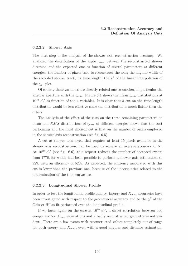
6.2 Reconstruction Accuracy andDefinition Of Analysis Cuts
6.2.2.2 Shower Axis
The next step is the analysis of the shower axis reconstruction accuracy. We
analyzed the distribution of the angle ηaxis between the reconstructed shower
direction and the expected one as function of several parameters at different
energies: the number of pixels used to reconstruct the axis; the angular width of
the recorded shower track; its time length; the χ2 of the linear interpolation of
the χi−plot.
Of course, these variables are directly related one to another, in particular the
angular aperture with the ηaxis. Figure 6.4 shows the mean ηaxis distributions at
1019 eV as function of the 4 variables. It is clear that a cut on the time length
distribution would be less effective since the distribution is much flatter then the
others.
The analysis of the effect of the cuts on the three remaining parameters on
mean and RMS distributions of ηaxis at different energies shows that the best
performing and the most efficient cut is that on the number of pixels employed
in the shower axis reconstruction (see fig. 6.5).
A cut at shower axis level, that requires at least 15 pixels available in the
shower axis reconstruction, can be used to achieve an average accuracy of 5.
At 1019 eV (see fig. 6.6), this request reduces the number of accepted events
from 1776, for which had been possible to perform a shower axis estimation, to
929, with an efficiency of 52%. As expected, the efficiency associated with this
cut is lower than the previous one, because of the uncertainties related to the
determination of the time curvature.
6.2.2.3 Longitudinal Shower Profile
In order to test the longitudinal profile quality, Energy and Xmax accuracies have
been investigated with respect to the geometrical accuracy and to the χ2 of the
Gaisser-Hillas fit performed over the longitudinal profile.
If we focus again on the case at 1019 eV , a direct correlation between bad
energy and/or Xmax estimations and a badly reconstructed geometry is not evi-
dent. There are a few events with reconstructed values completely out of range
for both energy and Xmax, even with a good angular and distance estimation.
160
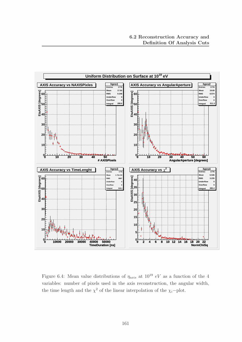
6.2 Reconstruction Accuracy andDefinition Of Analysis Cuts
eV19Uniform Distribution on Surface at 10
# AXISPixels0 10 20 30 40 50
hpro1Entries 1776
Mean 17.93
RMS 9.348
Underflow 0
Overflow 0
Integral 288.6
# AXISPixels0 10 20 30 40 50
Eta
AX
IS [
deg
rees
]
0
10
20
30
40
50
60
hpro1Entries 1776
Mean 17.93
RMS 9.348
Underflow 0
Overflow 0
Integral 288.6
AXIS Accuracy vs NAXISPixles
AngularAperture [degrees] 0 10 20 30 40 50 60
hpro2Entries 1776
Mean 19.69
RMS 8.574
Underflow 0
Overflow 0
Integral 511.3
AngularAperture [degrees] 0 10 20 30 40 50 60
Eta
AX
IS [
deg
rees
]
0
10
20
30
40
50
60
hpro2Entries 1776
Mean 19.69
RMS 8.574
Underflow 0
Overflow 0
Integral 511.3
AXIS Accuracy vs AngularAperture
TimeDuration [ns] 0 10000 20000 30000 40000 50000
hpro3Entries 1776
Mean 1.72e+04
RMS 8867
Underflow 0
Overflow 0
Integral 529.1
TimeDuration [ns] 0 10000 20000 30000 40000 50000
Eta
AX
IS [
deg
rees
]
0
10
20
30
40
50
60
hpro3Entries 1776
Mean 1.72e+04
RMS 8867
Underflow 0
Overflow 0
Integral 529.1
AXIS Accuracy vs TimeLenght
NormChiSq 0 2 4 6 8 10 12 14 16 18 20 22
hpro4Entries 1776
Mean 6.546
RMS 3.235
Underflow 0
Overflow 0
Integral 385.4
NormChiSq 0 2 4 6 8 10 12 14 16 18 20 22
Eta
AX
IS [
deg
rees
]
0
5
10
15
20
25
30
35
40
hpro4Entries 1776
Mean 6.546
RMS 3.235
Underflow 0
Overflow 0
Integral 385.4
2χAXIS Accuracy vs
Figure 6.4: Mean value distributions of ηaxis at 1019 eV as a function of the 4
variables: number of pixels used in the axis reconstruction, the angular width,
the time length and the χ2 of the linear interpolation of the χi−plot.
161
6.2 Reconstruction Accuracy andDefinition Of Analysis Cuts
Figure 6.5: Distribution of ηaxis mean (left panel) and rms (right panel) as a
function of the energy obtained by requiring 17 (blue ), 15 pixels (red ) and 6
(red ) for the angular width, the number of pixels used in the axis determination
and the χ2, respectively.
Events with an estimated Xmax out of range are mostly the same for which the
energy estimation is incorrect.
The dependence of energy and Xmax accuracy on the χ2 of the Gaisser-Hillas
fit has been investigated. The study has shown that it is difficult to fix a univocal
cut on the whole energy range.
A very useful cut, able to clean energy and Xmax distributions with an high
efficiency, is the request that the reconstructed Xmax is within the detector field
of view. Applying this cut (see figs. 6.7 and 6.8), events whose energy and Xmax
estimations out of range are removed, reducing the number of events to 812 for
the case of simulated shower at 1019 eV , with an efficency of 87%. This simple
geometrical cut allows to achieve an Xmax accuracy of ∼ 50 g/cm2 and of 5% in
energy.
162
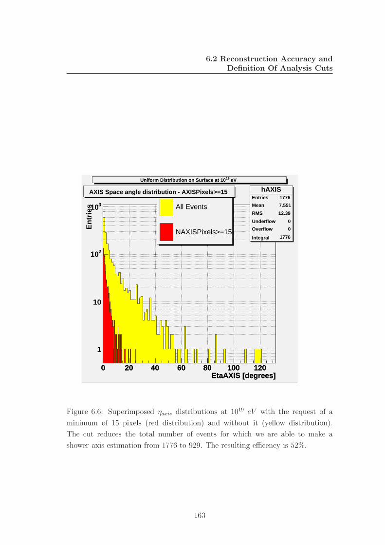
6.2 Reconstruction Accuracy andDefinition Of Analysis Cuts
eV 19Uniform Distribution on Surface at 10
EtaAXIS [degrees]0 20 40 60 80 100 120
hAXISEntries 1776
Mean 7.551
RMS 12.39
Underflow 0
Overflow 0
Integral 1776
EtaAXIS [degrees]0 20 40 60 80 100 120
En
trie
s
1
10
210
310
hAXISEntries 1776
Mean 7.551
RMS 12.39
Underflow 0
Overflow 0
Integral 1776
All Events
NAXISPixels>=15
AXIS Space angle distribution - AXISPixels>=15
Figure 6.6: Superimposed ηaxis distributions at 1019 eV with the request of a
minimum of 15 pixels (red distribution) and without it (yellow distribution).
The cut reduces the total number of events for which we are able to make a
shower axis estimation from 1776 to 929. The resulting efficency is 52%.
163
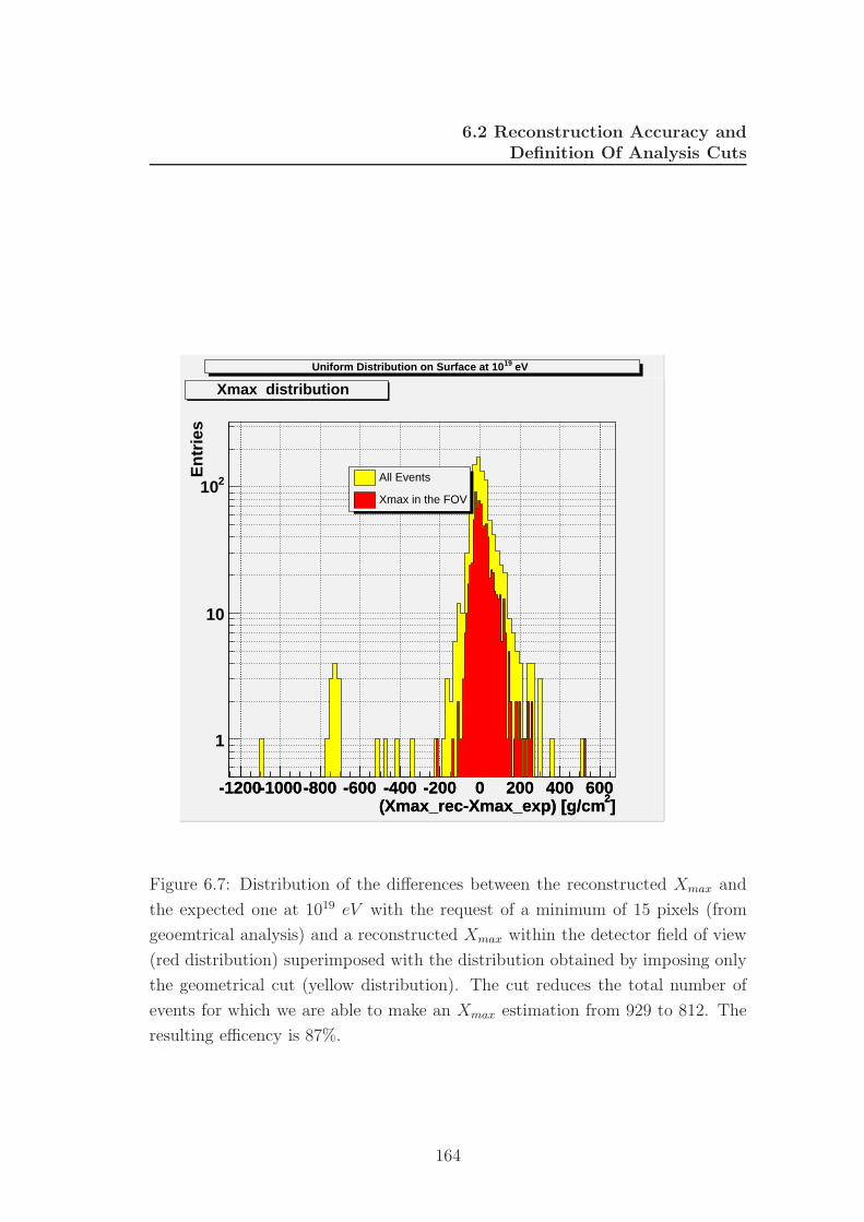
6.2 Reconstruction Accuracy andDefinition Of Analysis Cuts
eV 19Uniform Distribution on Surface at 10
]2(Xmax_rec-Xmax_exp) [g/cm-1200-1000-800 -600 -400 -200 0 200 400 600
]2(Xmax_rec-Xmax_exp) [g/cm-1200-1000-800 -600 -400 -200 0 200 400 600
En
trie
s
1
10
210
Xmax distribution
All Events
Xmax in the FOV
Figure 6.7: Distribution of the differences between the reconstructed Xmax and
the expected one at 1019 eV with the request of a minimum of 15 pixels (from
geoemtrical analysis) and a reconstructed Xmax within the detector field of view
(red distribution) superimposed with the distribution obtained by imposing only
the geometrical cut (yellow distribution). The cut reduces the total number of
events for which we are able to make an Xmax estimation from 929 to 812. The
resulting efficency is 87%.
164
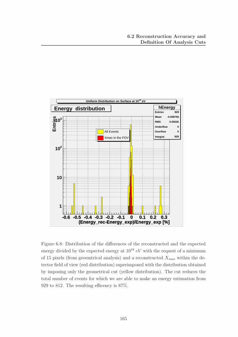
6.2 Reconstruction Accuracy andDefinition Of Analysis Cuts
eV 19Uniform Distribution on Surface at 10
(Energy_rec-Energy_exp)/Energy_exp [%]-0.6 -0.5 -0.4 -0.3 -0.2 -0.1 0 0.1 0.2 0.3
hEnergyEntries 929
Mean -0.008756
RMS 0.05636
Underflow 0
Overflow 0
Integral 929
(Energy_rec-Energy_exp)/Energy_exp [%]-0.6 -0.5 -0.4 -0.3 -0.2 -0.1 0 0.1 0.2 0.3
En
trie
s
1
10
210
310
hEnergyEntries 929
Mean -0.008756
RMS 0.05636
Underflow 0
Overflow 0
Integral 929
All Events
Xmax in the FOV
Energy distribution
Figure 6.8: Distribution of the differences of the reconstructed and the expected
energy divided by the expected energy at 1019 eV with the request of a minimum
of 15 pixels (from geoemtrical analysis) and a reconstructed Xmax within the de-
tector field of view (red distribution) superimposed with the distribution obtained
by imposing only the geometrical cut (yellow distribution). The cut reduces the
total number of events for which we are able to make an energy estimation from
929 to 812. The resulting efficency is 87%.
165
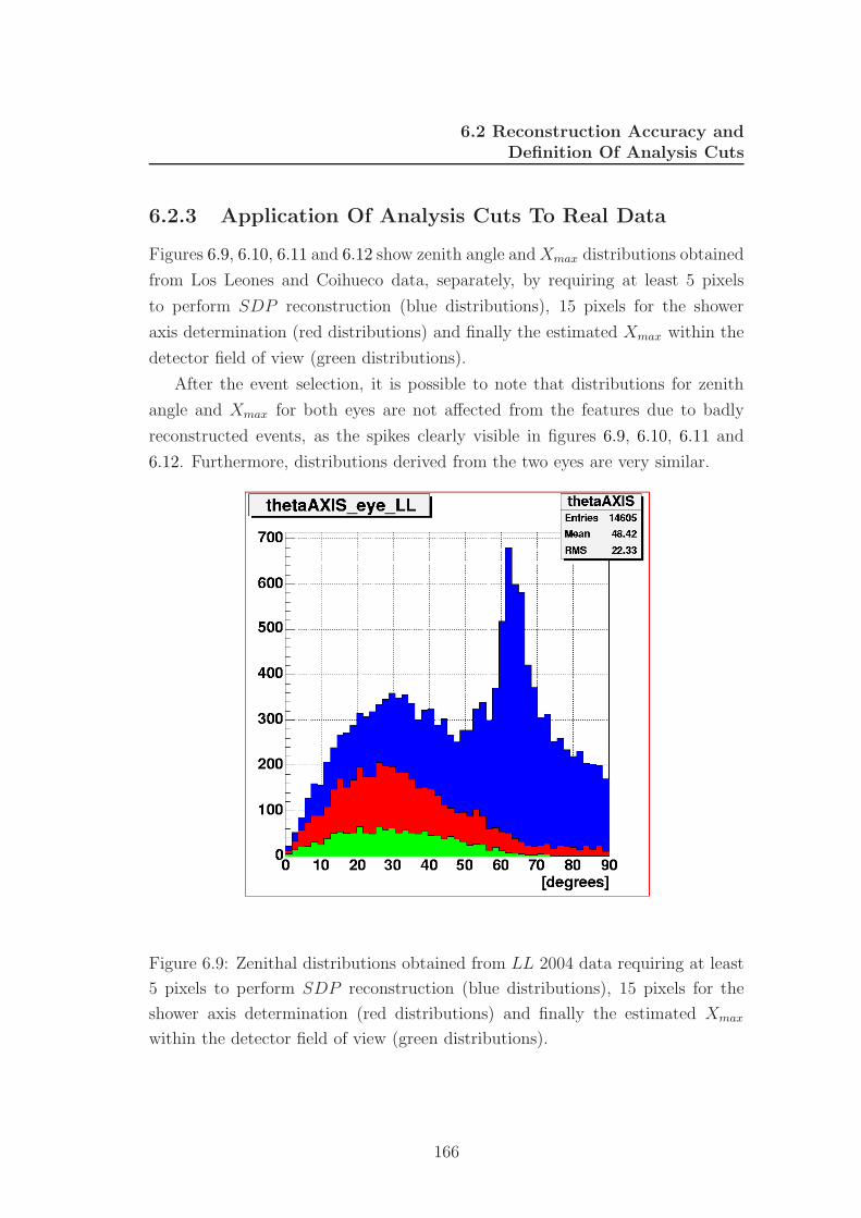
6.2 Reconstruction Accuracy andDefinition Of Analysis Cuts
6.2.3 Application Of Analysis Cuts To Real Data
Figures 6.9, 6.10, 6.11 and 6.12 show zenith angle and Xmax distributions obtained
from Los Leones and Coihueco data, separately, by requiring at least 5 pixels
to perform SDP reconstruction (blue distributions), 15 pixels for the shower
axis determination (red distributions) and finally the estimated Xmax within the
detector field of view (green distributions).
After the event selection, it is possible to note that distributions for zenith
angle and Xmax for both eyes are not affected from the features due to badly
reconstructed events, as the spikes clearly visible in figures 6.9, 6.10, 6.11 and
6.12. Furthermore, distributions derived from the two eyes are very similar.
Figure 6.9: Zenithal distributions obtained from LL 2004 data requiring at least
5 pixels to perform SDP reconstruction (blue distributions), 15 pixels for the
shower axis determination (red distributions) and finally the estimated Xmax
within the detector field of view (green distributions).
166
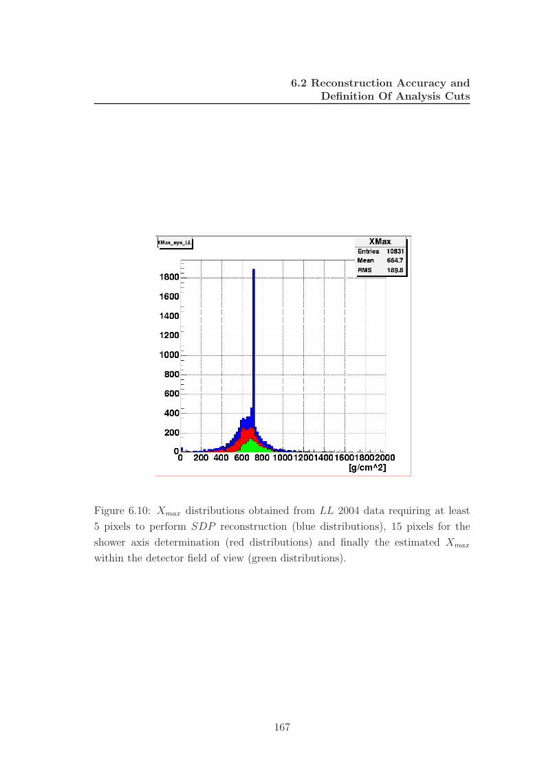
6.2 Reconstruction Accuracy andDefinition Of Analysis Cuts
Figure 6.10: Xmax distributions obtained from LL 2004 data requiring at least
5 pixels to perform SDP reconstruction (blue distributions), 15 pixels for the
shower axis determination (red distributions) and finally the estimated Xmax
within the detector field of view (green distributions).
167
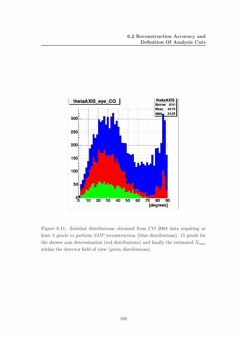
6.2 Reconstruction Accuracy andDefinition Of Analysis Cuts
Figure 6.11: Zenithal distributions obtained from CO 2004 data requiring at
least 5 pixels to perform SDP reconstruction (blue distributions), 15 pixels for
the shower axis determination (red distributions) and finally the estimated Xmax
within the detector field of view (green distributions).
168
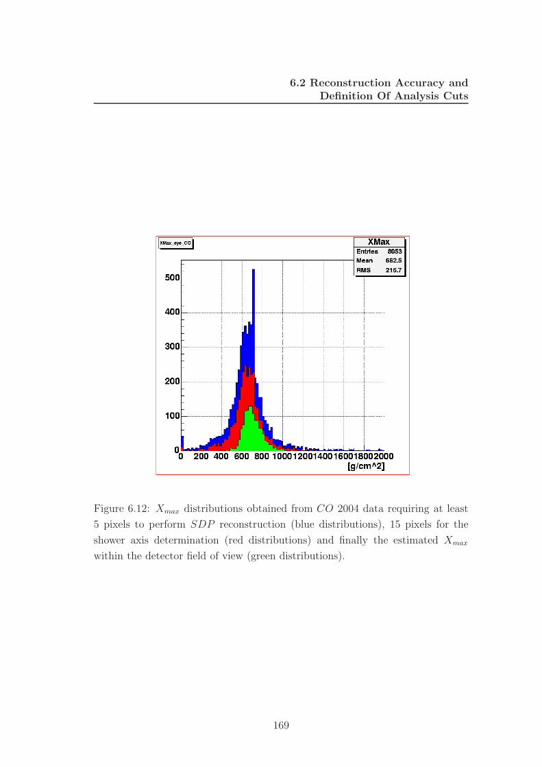
6.2 Reconstruction Accuracy andDefinition Of Analysis Cuts
Figure 6.12: Xmax distributions obtained from CO 2004 data requiring at least
5 pixels to perform SDP reconstruction (blue distributions), 15 pixels for the
shower axis determination (red distributions) and finally the estimated Xmax
within the detector field of view (green distributions).
169
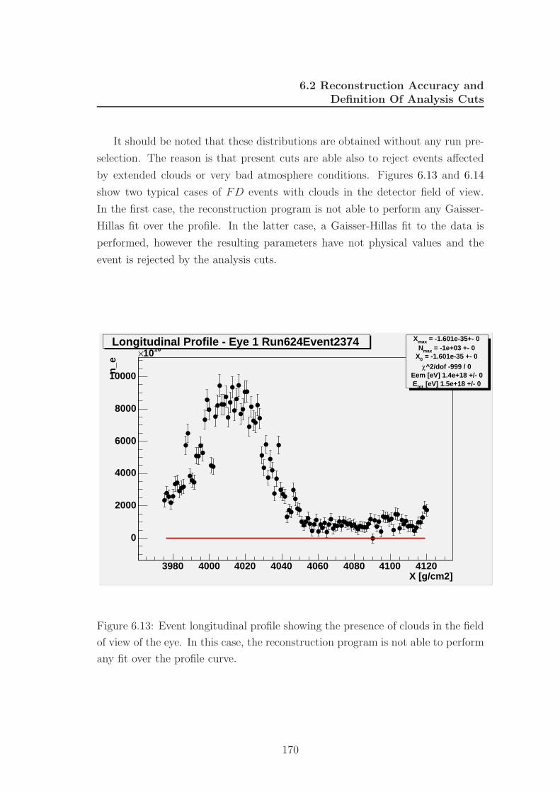
6.2 Reconstruction Accuracy andDefinition Of Analysis Cuts
It should be noted that these distributions are obtained without any run pre-
selection. The reason is that present cuts are able also to reject events affected
by extended clouds or very bad atmosphere conditions. Figures 6.13 and 6.14
show two typical cases of FD events with clouds in the detector field of view.
In the first case, the reconstruction program is not able to perform any Gaisser-
Hillas fit over the profile. In the latter case, a Gaisser-Hillas fit to the data is
performed, however the resulting parameters have not physical values and the
event is rejected by the analysis cuts.
X [g/cm2]3980 4000 4020 4040 4060 4080 4100 4120
n_e
0
2000
4000
6000
8000
10000
1010× = -1.601e-35+- 0maxX
= -1e+03 +- 0maxN = -1.601e-35 +- 00X
^2/dof -999 / 0χEem [eV] 1.4e+18 +/- 0
[eV] 1.5e+18 +/- 0totE
Longitudinal Profile - Eye 1 Run624Event2374
Figure 6.13: Event longitudinal profile showing the presence of clouds in the field
of view of the eye. In this case, the reconstruction program is not able to perform
any fit over the profile curve.
170
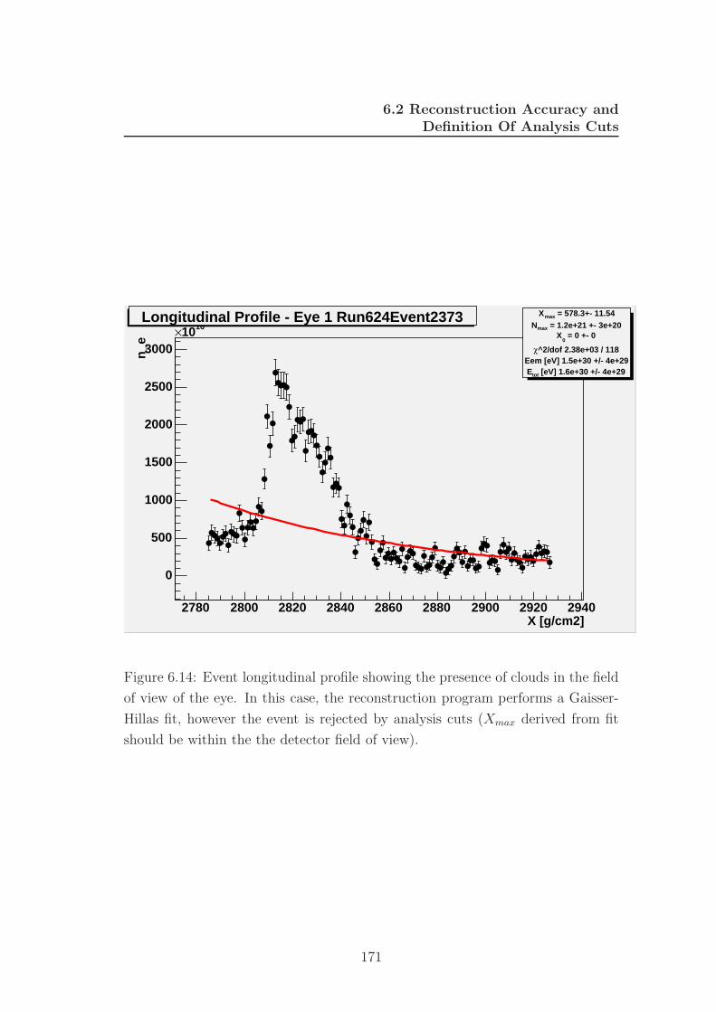
6.2 Reconstruction Accuracy andDefinition Of Analysis Cuts
X [g/cm2]2780 2800 2820 2840 2860 2880 2900 2920 2940
n_e
0
500
1000
1500
2000
2500
3000
1010× = 578.3+- 11.54maxX
= 1.2e+21 +- 3e+20maxN = 0 +- 0
0X
^2/dof 2.38e+03 / 118χEem [eV] 1.5e+30 +/- 4e+29
[eV] 1.6e+30 +/- 4e+29totE
Longitudinal Profile - Eye 1 Run624Event2373
Figure 6.14: Event longitudinal profile showing the presence of clouds in the field
of view of the eye. In this case, the reconstruction program performs a Gaisser-
Hillas fit, however the event is rejected by analysis cuts (Xmax derived from fit
should be within the the detector field of view).
171
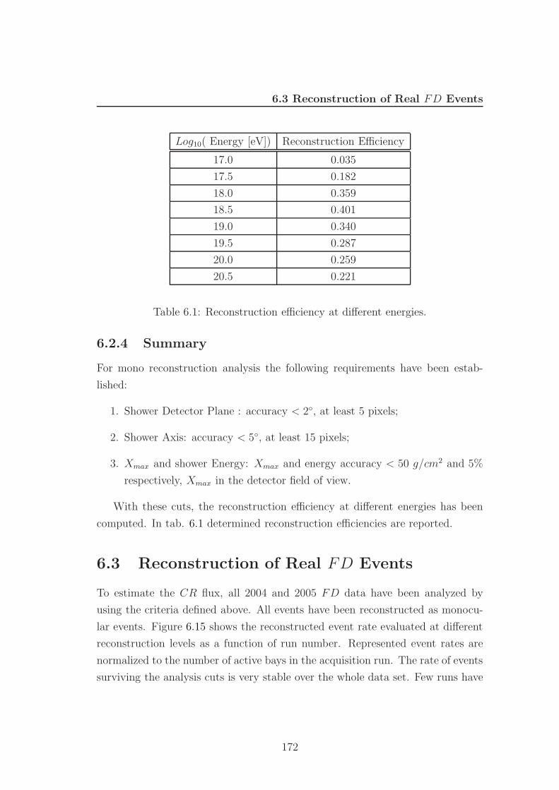
6.3 Reconstruction of Real FD Events
Log10( Energy [eV]) Reconstruction Efficiency
17.0 0.035
17.5 0.182
18.0 0.359
18.5 0.401
19.0 0.340
19.5 0.287
20.0 0.259
20.5 0.221
Table 6.1: Reconstruction efficiency at different energies.
6.2.4 Summary
For mono reconstruction analysis the following requirements have been estab-
lished:
1. Shower Detector Plane : accuracy < 2, at least 5 pixels;
2. Shower Axis: accuracy < 5, at least 15 pixels;
3. Xmax and shower Energy: Xmax and energy accuracy < 50 g/cm2 and 5%
respectively, Xmax in the detector field of view.
With these cuts, the reconstruction efficiency at different energies has been
computed. In tab. 6.1 determined reconstruction efficiencies are reported.
6.3 Reconstruction of Real FD Events
To estimate the CR flux, all 2004 and 2005 FD data have been analyzed by
using the criteria defined above. All events have been reconstructed as monocu-
lar events. Figure 6.15 shows the reconstructed event rate evaluated at different
reconstruction levels as a function of run number. Represented event rates are
normalized to the number of active bays in the acquisition run. The rate of events
surviving the analysis cuts is very stable over the whole data set. Few runs have
172
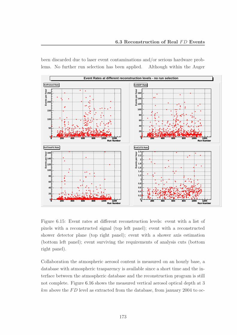
6.3 Reconstruction of Real FD Events
been discarded due to laser event contaminations and/or serious hardware prob-
lems. No further run selection has been applied. Although within the Auger
Event Rates at different reconstruction levels - no run selection
Run Number0 200 400 600 800 1000 1200
Run Number0 200 400 600 800 1000 1200
Eve
nts
per
ho
ur
0
50
100
150
200
250
EvtPulsed Rate
Run Number0 200 400 600 800 1000 1200
Run Number0 200 400 600 800 1000 1200
Eve
nts
per
ho
ur
0
20
40
60
80
100
120
140
160
EvtSDP Rate
Run Number0 200 400 600 800 1000 1200
Run Number0 200 400 600 800 1000 1200
Eve
nts
per
ho
ur
0
20
40
60
80
100
120
140
160
EvtTimeFit Rate
Run Number0 200 400 600 800 1000 1200
Run Number0 200 400 600 800 1000 1200
Eve
nts
per
ho
ur
0
0.2
0.4
0.6
0.8
1
1.2
1.4
1.6
1.8
2
2.2
2.4
EvtCUTS Rate
Figure 6.15: Event rates at different reconstruction levels: event with a list of
pixels with a reconstructed signal (top left panel); event with a reconstructed
shower detector plane (top right panel); event with a shower axis estimation
(bottom left panel); event surviving the requirements of analysis cuts (bottom
right panel).
Collaboration the atmospheric aerosol content is measured on an hourly base, a
database with atmospheric trasparency is available since a short time and the in-
terface between the atmospheric database and the reconstruction program is still
not complete. Figure 6.16 shows the measured vertical aerosol optical depth at 3
km above the FD level as extracted from the database, from january 2004 to oc-
173
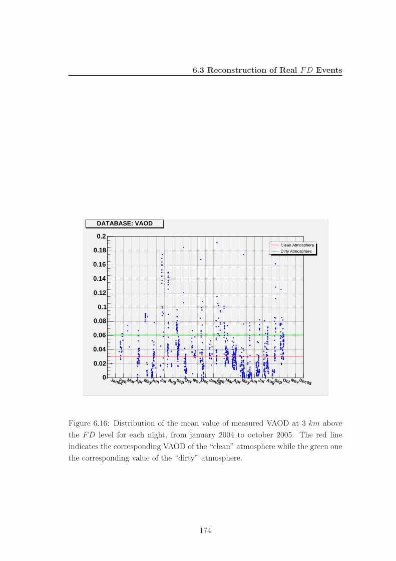
6.3 Reconstruction of Real FD Events
Jan04Feb Mar Apr MayJun Jul AugSepOct NovDec Jan05
Feb Mar Apr MayJun Jul AugSep Oct Nov Dec050
0.02
0.04
0.06
0.08
0.1
0.12
0.14
0.16
0.18
0.2
DATABASE: VAOD
Clean Atmosphere
Dirty Atmosphere
DATABASE: VAOD
Figure 6.16: Distribution of the mean value of measured VAOD at 3 km above
the FD level for each night, from january 2004 to october 2005. The red line
indicates the corresponding VAOD of the “clean” atmosphere while the green one
the corresponding value of the “dirty” atmosphere.
174
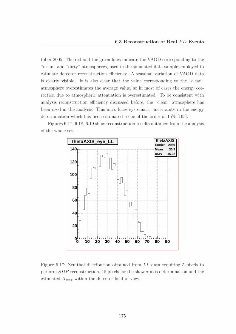
6.3 Reconstruction of Real FD Events
tober 2005. The red and the green lines indicate the VAOD corresponding to the
“clean” and “dirty” atmospheres, used in the simulated data sample employed to
estimate detector reconstruction efficiency. A seasonal variation of VAOD data
is clearly visible. It is also clear that the value corresponding to the “clean”
atmosphere overestimates the average value, so in most of cases the energy cor-
rection due to atmospheric attenuation is overestimated. To be consistent with
analysis reconstruction efficiency discussed before, the “clean” atmosphere has
been used in the analysis. This introduces systematic uncertainty in the energy
determination which has been estimated to be of the order of 15% [165].
Figures 6.17, 6.18, 6.19 show reconstruction results obtained from the analysis
of the whole set.
0 10 20 30 40 50 60 70 80 900 10 20 30 40 50 60 70 80 900
20
40
60
80
100
120
140
thetaAXIS_eye_LL thetaAXISEntries 2959Mean 30.9
RMS 15.02
thetaAXIS_eye_LL
Figure 6.17: Zenithal distribution obtained from LL data requiring 5 pixels to
perform SDP reconstruction, 15 pixels for the shower axis determination and the
estimated Xmax within the detector field of view.
175
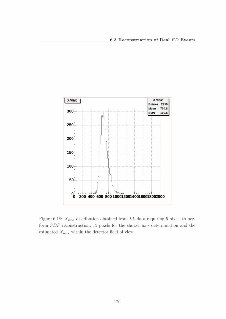
6.3 Reconstruction of Real FD Events
0 200 400 600 800 1000120014001600180020000 200 400 600 800 1000120014001600180020000
50
100
150
200
250
300
XMax XMaxEntries 2959Mean 704.8
RMS 100.5
XMax
Figure 6.18: Xmax distribution obtained from LL data requiring 5 pixels to per-
form SDP reconstruction, 15 pixels for the shower axis determination and the
estimated Xmax within the detector field of view.
176
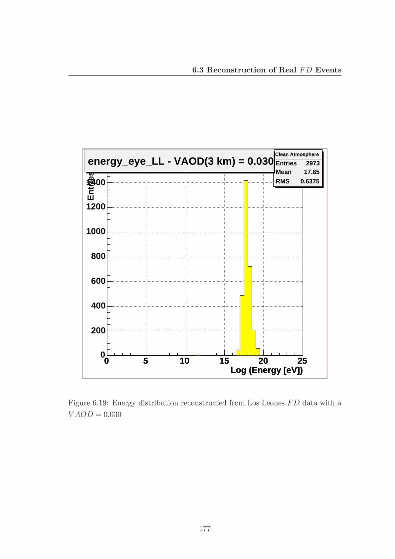
6.3 Reconstruction of Real FD Events
Log (Energy [eV])0 5 10 15 20 25
Clean Atmosphere
Entries 2973Mean 17.85
RMS 0.6375
Log (Energy [eV])0 5 10 15 20 25
En
trie
s
0
200
400
600
800
1000
1200
1400
Clean Atmosphere
Entries 2973Mean 17.85
RMS 0.6375
energy_eye_LL - VAOD(3 km) = 0.030
Figure 6.19: Energy distribution reconstructed from Los Leones FD data with a
V AOD = 0.030
177
6.4 Analysis Results
6.4 Analysis Results
6.4.1 All Particle Spectrum
In an ideal case in which detector configuration, detector efficiency and at-
mospheric conditions do not depend on time, the CR flux in the energy bin
[E, E + dE] is given by
φ(E) =N(E)
Aperture(E) · LiveTime · ReconstructionEfficiency(E) · E (6.1)
where N(E) is the number of events recorded with energy in the selected
energy bin.
In a more realistic case, for an estimation of the CR flux with the FD detec-
tor, these terms and their dependence on time, atmospheric conditions, shower
geometry, primary mass compositions, Monte Carlo, etc, have to be taken into
account.
1. Detector Aperture. FD detector has the great advantage with respect to
the ground array to have a direct energy calibration. But the detector has
not a fixed aperture. The fluorescence detector aperture grows up with the
energy and depends on atmospheric conditions during data taking. As a
consequence, the detector aperture should to be studied as a function of the
energy in different atmospheric conditions and possible detector configura-
tions. Of course, its dependence on primary mass composition and Monte
Carlo codes should be also considered.
2. Time Exposure. For each FD eye, data acquisition time should be com-
puted. Detector status should be continously monitored. FD acquisition
status could be different night by night, hour by hour, because one or more
of telescopes could be out of operations for a certain time interval during
a night. The computing of the detector live time has to take into account
the possible different status of data acquisition.
3. Reconstruction Efficiency. Once a set of analysis cut is fixed, it is possible
to obtain a detailed knowledge of the reconstruction efficiency at different
energies.
178
6.4 Analysis Results
In section 6.2, I have already computed the reconstruction efficiency at dif-
ferent energies. To evaluate the determinator of eq. 6.1 in a realistic case, all
possible configurations of an FD eye must be considered. The eye acquisition
configuration can be described by a pattern of active telescopes defined as a 6−bit
word. For instance, if there are 4 active telescopes, bay1, bay2, bay5, bay6, the
pattern will be 1,1,0,0,1,1. There are 64 possible patterns. In addition, tele-
scopes have been equipped with corrector rings at different times. From january
2004 to november 2005, four periods can be distinguished. Therefore the term
Aperture(E) · LiveTime · ReconstructionEfficiency(E) (6.2)
can be expressed as4∑
j=1
64∑i=1
Ai,j(E) · Ti,j · εi,j (6.3)
where the sum is performed over the 26 configurations of active bays, Ai,j(E),
Ti,j and εi,j are aperture, live time and reconstruction efficiency of each configu-
ration, respectively.
Next sections will be devoted to discuss the detector aperture and the deter-
mination of the detector live time.
6.4.1.1 Detector Aperture
Within the Auger Collaboration, two sets of simulated showers have been pro-
duced in order to estimate the detector aperture. The first one uses a parametriza-
tion of longitudinal profiles of air showers, that allows to simulate shower profiles
at each energy in a fast way, avoiding the use of a complex and heavier simu-
lation code like CORSIKA. By using these simulated showers, L’Aquila Auger
group made a detailed study of the FD detector trigger aperture [178]. Detector
response has been checked in different conditions:
1. Two different shower cores ditributions. Showers have been produced uni-
formely in distance and in area, within the field of view of a single telescope,
bay4 of the Los Leones eye and up to distance from the eye that depends
on the energy (6 km at 1017 eV up to 80 km for E > 1019.5 eV ). The
reason for this is to evaluate detector response at different distances with
179
6.4 Analysis Results
high statistics (uniform in distance) and its behavior in the more realistic
case of a uniform distribution of shower cores (uniform in area).
2. Two different atmospheric conditions. To investigate the dependence of the
detector aperture on atmospheric conditions the “clean” and the “dirty”
atmospheres, defined above, have been employed
3. Two primary particles. Simulated showers are produced for proton and iron
primaries, in order to estimate the aperture dependence on comic ray mass
composition.
4. Two telescope configurations. A growing fraction of Auger FD telescopes
makes use of corrector rings to enhance their aperture without introducing
optical aberrations. To understand the effect on detector aperture both
configurations, with and without them, have been investigated.
For each possible combination of these parameters, 10000 simulate showers have
been produced at fixed values of Log(E/eV ) = 17, 17.5, 18, 18.5, 19, 19.5, 20,
20.5, with zenith angle within 60 degrees, with a cos θd(cos θ) zenith distribution
and uniform azimuth distribution. The aperture trigger function is computed
with a semi-analytical approach: a single telescope aperture is computed with
high statistics and is analytically generalized to the whole eye.
Recently - November 2005 - a second set has been completed by using the
CORSIKA Monte Carlo and it is composed by [190]:
1. 50000 proton showers;
2. energy spectrum from 1017.5 eV to 1020.5 eV , according to dN/dE ∝ E−1;
3. zenith distribution from 0 to 60, according to dN/(d cos θ) ∝ cos θ;
4. uniformely distributed over an area of 80 km × 80 km.
5. showers propagate through the “clean” atmosphere.
6. FD telescopes with corrector rings.
180
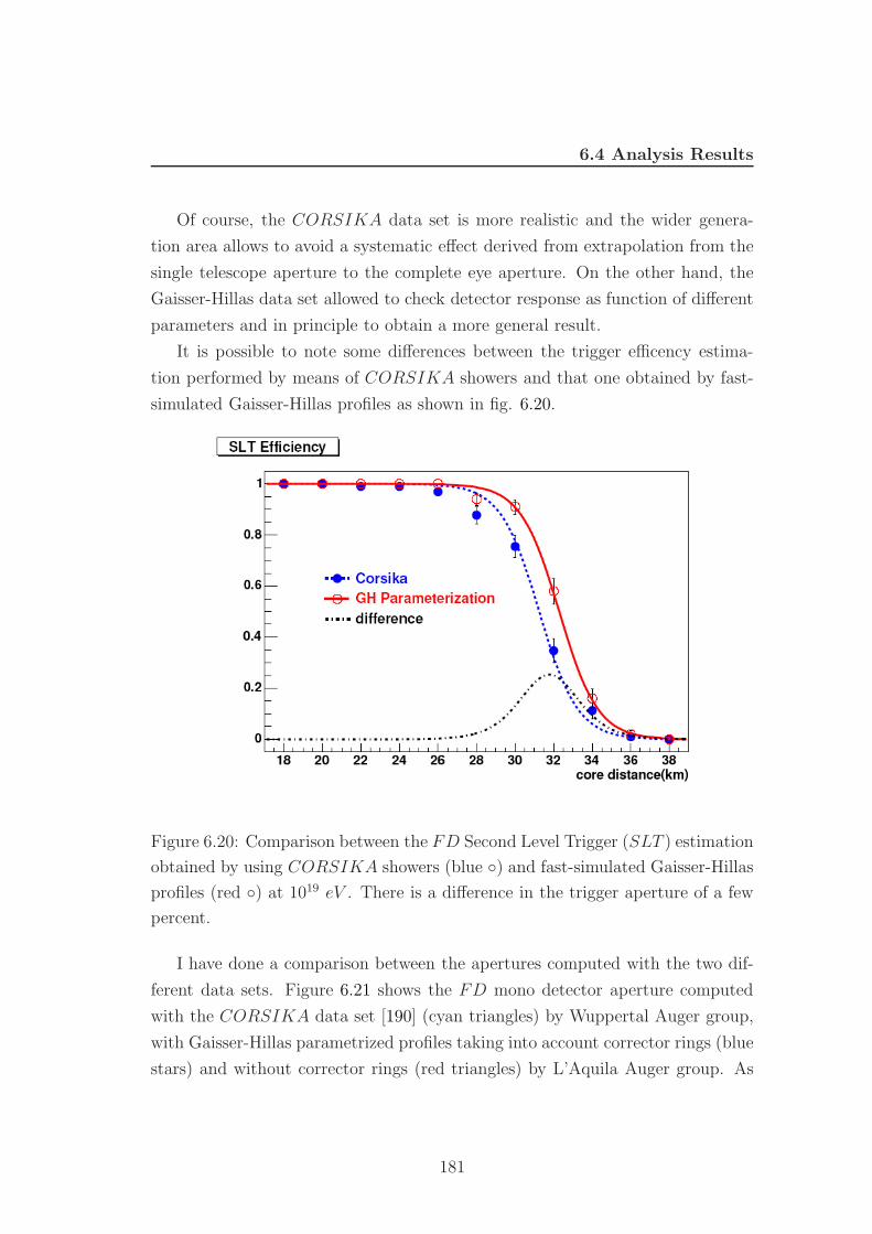
6.4 Analysis Results
Of course, the CORSIKA data set is more realistic and the wider genera-
tion area allows to avoid a systematic effect derived from extrapolation from the
single telescope aperture to the complete eye aperture. On the other hand, the
Gaisser-Hillas data set allowed to check detector response as function of different
parameters and in principle to obtain a more general result.
It is possible to note some differences between the trigger efficency estima-
tion performed by means of CORSIKA showers and that one obtained by fast-
simulated Gaisser-Hillas profiles as shown in fig. 6.20.
Figure 6.20: Comparison between the FD Second Level Trigger (SLT ) estimation
obtained by using CORSIKA showers (blue ) and fast-simulated Gaisser-Hillas
profiles (red ) at 1019 eV . There is a difference in the trigger aperture of a few
percent.
I have done a comparison between the apertures computed with the two dif-
ferent data sets. Figure 6.21 shows the FD mono detector aperture computed
with the CORSIKA data set [190] (cyan triangles) by Wuppertal Auger group,
with Gaisser-Hillas parametrized profiles taking into account corrector rings (blue
stars) and without corrector rings (red triangles) by L’Aquila Auger group. As
181
6.4 Analysis Results
expected, the use of correcor rings enlarges detector aperture. Wuppertal results
are systematically higher than L’Aquila ones. Part of the discrepancy is due to
the effect already shown in figure 6.20 in a particular case. Another contribution
is due to a systematic underestimate of the simple semi-analytical approach. A
more refined semi-analytical approach is under development.
It should be noted that both aperture determination are given in the ideal case
of the complete eye with all 6 telescopes in operation. In principle, the aperture of
each configuration should be computed, in absence of such a detailed information,
I used the reasonable assumption to scale down the total eye aperture by 1/6 for
each missing telescope. This does not take into account for correlations between
neighbouring telescopes.
6.4.1.2 Live Time Determination
In order to estimate the detector live time, I followed the detector evolution in
time.
In principle, different telescope configurations could characterize a run, be-
cause during data acquisition some bay could go out of operation for hardware
problems, or their shutters may be closed when the moon is in their field of view.
The latter case may happen at the start, at the end and during the run. Then for
each run, the active telescope patterns and their live time have been computed.
A continous scan of active bays is performed: at each second the eye data taking
configuration pattern is checked and is corresponding live time is incremented.
In this way, 64 eye patterns for the four time periods corresponding to corrector
ring commissioning, live time values are computed.
6.4.1.3 Spectrum Evaluation
Reconstruction efficiency and detector aperture are measured at a fixed energy in
steps of 100.5 eV . So, FD data will be grouped in 8 energy intervals ([16.75, 17.25[
and so on). Since efficiency and aperture estimation have been extracted from a
data sample with a zenith angle lower than 60 degrees, events with zenith angle
higher than 60 have been rejected. With this binning each energy interval is
much wider than energy bins of existing data. To perform a comparison, the flux
182
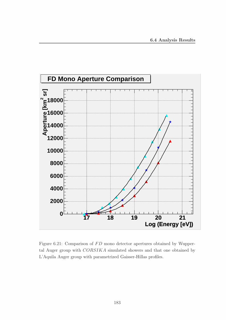
6.4 Analysis Results
Log (Energy [eV])17 18 19 20 21
Log (Energy [eV])17 18 19 20 21
sr]
2A
per
ture
[km
0
2000
4000
6000
8000
10000
12000
14000
16000
18000
FD Mono Aperture Comparison
Figure 6.21: Comparison of FD mono detector apertures obtained by Wupper-
tal Auger group with CORSIKA simulated showers and that one obtained by
L’Aquila Auger group with parametrized Gaisser-Hillas profiles.
183
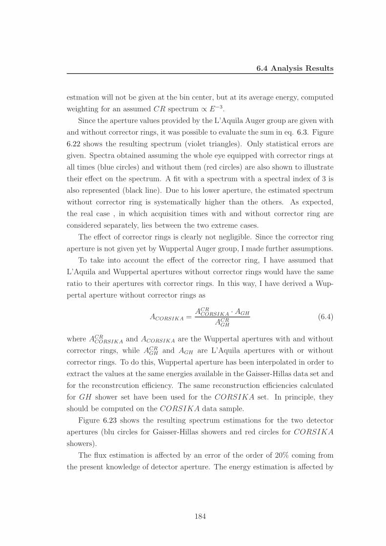
6.4 Analysis Results
estmation will not be given at the bin center, but at its average energy, computed
weighting for an assumed CR spectrum ∝ E−3.
Since the aperture values provided by the L’Aquila Auger group are given with
and without corrector rings, it was possible to evaluate the sum in eq. 6.3. Figure
6.22 shows the resulting spectrum (violet triangles). Only statistical errors are
given. Spectra obtained assuming the whole eye equipped with corrector rings at
all times (blue circles) and without them (red circles) are also shown to illustrate
their effect on the spectrum. A fit with a spectrum with a spectral index of 3 is
also represented (black line). Due to his lower aperture, the estimated spectrum
without corrector ring is systematically higher than the others. As expected,
the real case , in which acquisition times with and without corrector ring are
considered separately, lies between the two extreme cases.
The effect of corrector rings is clearly not negligible. Since the corrector ring
aperture is not given yet by Wuppertal Auger group, I made further assumptions.
To take into account the effect of the corrector ring, I have assumed that
L’Aquila and Wuppertal apertures without corrector rings would have the same
ratio to their apertures with corrector rings. In this way, I have derived a Wup-
pertal aperture without corrector rings as
ACORSIKA =ACR
CORSIKA · AGH
ACRGH
(6.4)
where ACRCORSIKA and ACORSIKA are the Wuppertal apertures with and without
corrector rings, while ACRGH and AGH are L’Aquila apertures with or without
corrector rings. To do this, Wuppertal aperture has been interpolated in order to
extract the values at the same energies available in the Gaisser-Hillas data set and
for the reconstrcution efficiency. The same reconstruction efficiencies calculated
for GH shower set have been used for the CORSIKA set. In principle, they
should be computed on the CORSIKA data sample.
Figure 6.23 shows the resulting spectrum estimations for the two detector
apertures (blu circles for Gaisser-Hillas showers and red circles for CORSIKA
showers).
The flux estimation is affected by an error of the order of 20% coming from
the present knowledge of detector aperture. The energy estimation is affected by
184
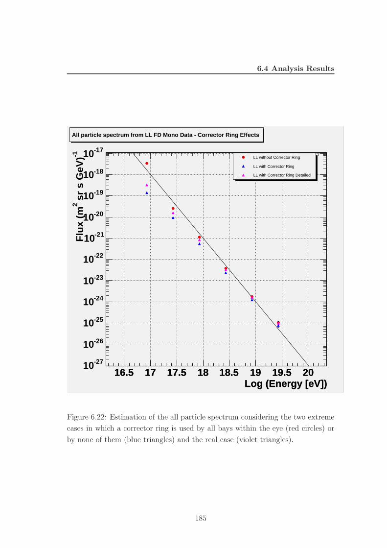
6.4 Analysis Results
Log (Energy [eV])16.5 17 17.5 18 18.5 19 19.5 20
Log (Energy [eV])16.5 17 17.5 18 18.5 19 19.5 20
-1 s
r s
GeV
)2
Flu
x (m
-2710
-2610
-2510
-2410
-2310
-2210
-2110
-2010
-1910
-1810
-1710 LL without Corrector Ring
LL with Corrector Ring
LL with Corrector Ring Detailed
All particle spectrum from LL FD Mono Data - Corrector Ring Effects
Figure 6.22: Estimation of the all particle spectrum considering the two extreme
cases in which a corrector ring is used by all bays within the eye (red circles) or
by none of them (blue triangles) and the real case (violet triangles).
185
6.4 Analysis Results
different systematic uncertainties (see section 3.6.3) mainly due to the fluores-
cence yield (∼ 15%), to the FD absolute calibration (∼ 12%) and to atmosphere
attenuation - Mie scattering - (15%). In addition, a further uncertainty of ∼ 15%
due to the use of fixed “clean” atmosphere in the data analysis should be in-
cluded. These ones, together with other smaller FD uncertainties, give a total
systematic uncertainty of the order of 30% in the energy. With these uncertain-
ties, it is possible to estimate the two extreme all particle spectra, reported in
fig. 6.24, which correspond to the aperture uncertainties, The figure also shows
the first Auger spectrum presented at ICRC 2005 [191], produced with only SD
data. Auger spectrum starts at higher energies with respect to this estimation
because the SD, in comparison with the FD, has an higher trigger threshold.
On the same plot, published spectra by AGASA and HiRes are also shown.
6.4.2 Elongation Rate
The distribution of positions of shower maximum (Xmax) in the atmosphere has
been shown to be sensitive to the composition of CRs. It is well known that for
any particular species of nucleus the position of shower maximum deepens with
increasing energy as the logarithm of the energy (see sec. 1.4.8.2). The slope
d(Xmax)/d(logE) is known as the elongation rate (De). While the details depend
on the hadronic model assumed, all modern hadronic models give approximately
the same De (between 50 and 60 g/cm2 per decade of energy, independent of
particle species) and agree within about 25 g/cm2 on the absolute position of the
average shower Xmax at a given energy for a given species. The sensitivity of the
Xmax method to composition comes from the fact that the mean Xmax for iron
and protons is different by about 80-100 g/cm2, independent of hadronic model,
with protons producing deeper showers with larger fluctuations. A change in
the composition from heavy to light would then result in a larger De than 50-60
g/cm2 per decade, and a change from light to heavy would lead to a lower and
even negative De.
The general dependence of Xmax on energy can be seen in a simple branching
model in which Nmax ∝ E0 and Xmax ∝ lnE0, where E0 is the primary cosmic
ray energy [85]. In this model if the primary particle is a nucleus, the shower
186
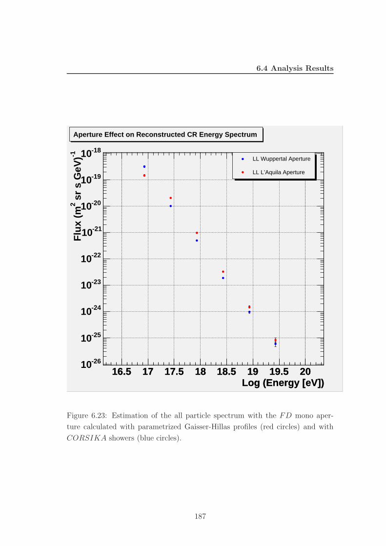
6.4 Analysis Results
Log (Energy [eV])16.5 17 17.5 18 18.5 19 19.5 20
Log (Energy [eV])16.5 17 17.5 18 18.5 19 19.5 20
-1 s
r s
GeV
)2
Flu
x (m
-2610
-2510
-2410
-2310
-2210
-2110
-2010
-1910
-1810LL Wuppertal Aperture
LL L’Aquila Aperture
Aperture Effect on Reconstructed CR Energy Spectrum
Figure 6.23: Estimation of the all particle spectrum with the FD mono aper-
ture calculated with parametrized Gaisser-Hillas profiles (red circles) and with
CORSIKA showers (blue circles).
187
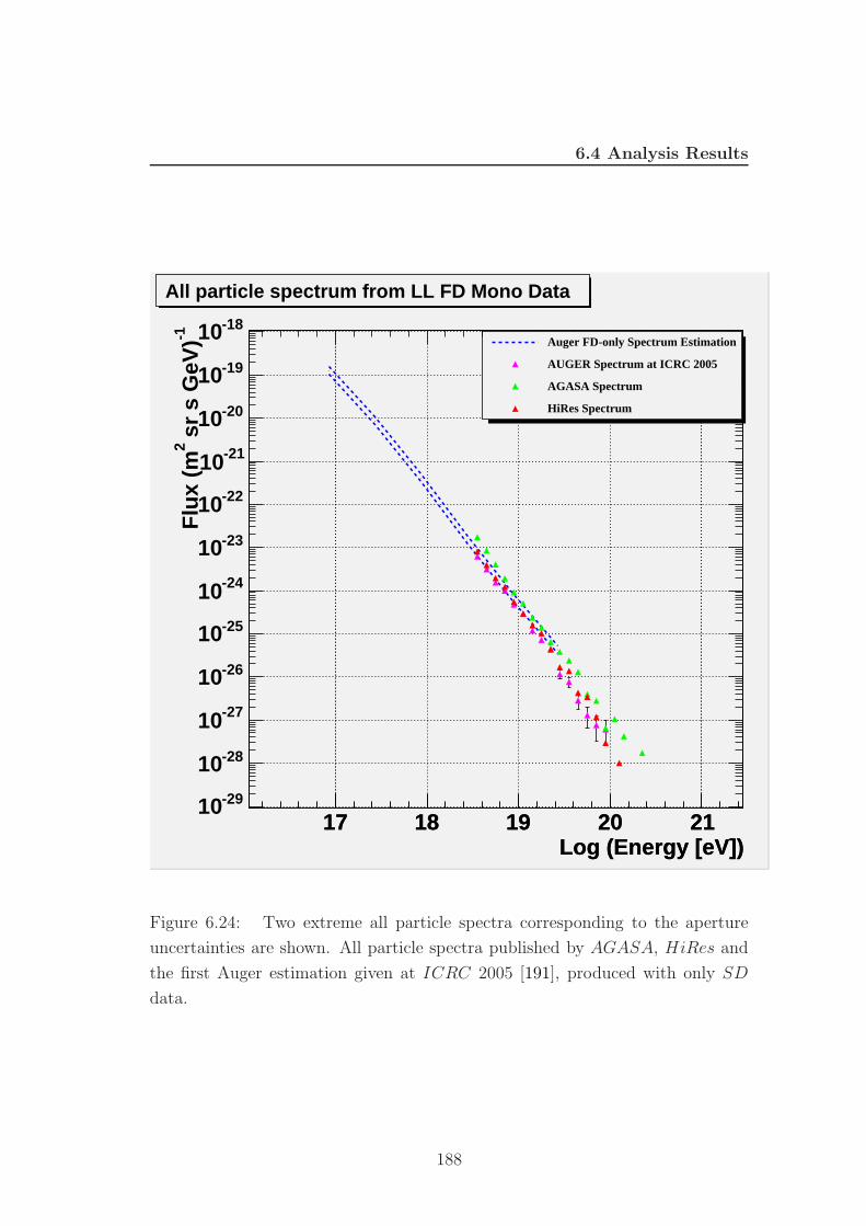
6.4 Analysis Results
Log (Energy [eV])17 18 19 20 21
Log (Energy [eV])17 18 19 20 21
-1 s
r s
GeV
)2
Flu
x (m
-2910
-2810
-2710
-2610
-2510
-2410
-2310
-2210
-2110
-2010
-1910
-1810 Auger FD-only Spectrum Estimation
AUGER Spectrum at ICRC 2005
AGASA Spectrum
HiRes Spectrum
All particle spectrum from LL FD Mono Data
Figure 6.24: Two extreme all particle spectra corresponding to the aperture
uncertainties are shown. All particle spectra published by AGASA, HiRes and
the first Auger estimation given at ICRC 2005 [191], produced with only SD
data.
188
6.4 Analysis Results
is assumed to be a superposition of subshowers, each initiated by one of the
A independent nucleons. The primary energy must be divided among the A
constituents, so in this case Xmax ∝ ln A × E0. A more complete discussion leads
to Linsley’s expression for the De:
De = X0(1 − B)
[1 − ð〈lnA〉
ð〈lnE〉]
(6.5)
It includes both the energy dependence of the cross section and the energy
dependence of the multiplicity and inelasticity.
The technique for extracting the CR composition used then reduces to com-
paring the Xmax distribution of the data after appropriate cuts that guarantee
good resolution in this variable, with simulated data generated with either a pro-
ton or iron parent particle. The simulated data are the result of a detector Monte
Carlo and include all the reconstruction uncertainties.
While CR hadronic composition presumably can range anywhere between the
two extremes of pure proton and pure Fe, the 30 g/cm2 resolution of the detector
and the existence of significant shower fluctuations lead us to compare the data
with a simplified two-component model. Events are generated using CORSIKA
6.005 and 6.010 [] and using QGSJet01 [] for high energy hadronic model and
GHEISHA for low energy hadronic model (> 80 GeV). In all simulations, the
CORSIKA EGS4 option is selected, enabling explicit treatment of each electro-
magnetic interaction for particles above a threshold energy. Electrons, positrons,
and photons were tracked down to energies of 100 keV. Hadrons and muons were
tracked to 300 MeV. The showers were initiated from 0 to 53 degree with sam-
pling at 5 g/cm2 of vertical atmospheric depth and the thinning level was set at
10−6. For this study 100 iron showers and 100 proton showers are used in each
0.5 step of log E from 1018 to 1020 eV (simulation were performed at the Lyon
Computer Center).
Figure 6.25 shows the preliminary elongation rate obtained with selected data
set (black stars), compared with those expected from the two extreme cases of
cosmic ray mass composition, proton or iron primary particles. Simulated re-
sults are presented taking into account detector and reconstruction effects (red
solid circles and blue solid squares for protons and irons, respectively). The red
189

6.4 Analysis Results
Log10(E[eV])17.5 18 18.5 19 19.5 20 20.5 21
Log10(E[eV])17.5 18 18.5 19 19.5 20 20.5 21
XM
ax [
g/c
m^2
]
600
650
700
750
800
850
900
protonironreal data
pure protonpure iron
ELONGATION RATE
Figure 6.25: Preliminary elongation rate estimation obtained with selected data
set (black stars), compared with those expected from the two extreme cases of cos-
mic ray mass composition, proton or iron primary particles, taking into account
detector effects (red solid circles and blue solid squares for protons and irons,
respectively) and not (red and blue lines for protons and irons, respectively).
190
6.5 Conclusions
and blue lines (protons and irons, respectively) are the results of CORSIKA
simulation without the filter of the Offline reconstruction
The preliminary elongation rate is, of course, affected by the same uncertain-
ties discussed on the energy determination. In addition, a further uncertainty on
Xmax determination of ∼ 30 g/cm2, mainly due to the knowledge of atmospheric
density profile, should be also included.
6.5 Conclusions
The spectrum presented in figure 6.24 is only the first attempt to build up a cosmic
ray spectrum with only FD data within the Auger Collaboration. It is affected by
different systematic uncertainties, on the energy determination (30%) and on the
detector aperture determination (20%). Only the two extreme spectra are given.
The work on this topic is still in progress. All the details of the calculation should
be refined, from the computing of the detector live time to the use of measured
atmospheric conditions, from the estimation of the reconstruction efficiency to
the detector aperture.
The presented elongation rate is only a preliminary estimation. The simulated
data set used to compare with real data is clearly limited. The estimation is
affected by systematic uncertainties, already discussed, on energy determination
and by further uncertainties related to the Xmax determination of ∼ 30 g/cm2,
due to the knowledge of atmospheric density profile.
191
Conclusions
The Pierre Auger Southern Observatory is going to be completed. Since septem-
ber 2003, the Observatory is recording extended air showers by means of two
independent and complementary detectors. In august 2005, the first shower has
been detected by 3 fluorescence 3. Within the Pierre Auger Collaboration, de-
tector features are studied with more and more details. Analysis tools are under
development and optimization.
In this scenery, I have studied details of Fluorescence detector event recon-
struction and new algorithms have been developed in order to enhance recon-
struction performances. The geometrical reconstruction of Fluorescence Detec-
tor events have been improved by implementing the use of gnomonic projections
to perform the first geometrical reconstruction step, the shower detector plane
determination. The new approach has been tested with very good results over a
wide set of simulated showers and laser shots. The study has also shown a visible
effects of the improved shower detector plane determination on the reconstruction
of shower energy and of the depth of shower maximum.
The improved Fluorescence detector geometrical reconstruction has been tested
by mean of laser shots of known geometry, in order to estimate reconstruction
accuracy. All possible event reconstruction typology have been tested (mono, hy-
brid and stereo). Results have shown an incomparable reconstruction accuracy.
In particular, the stereo reconstruction allows a very accurate core determination.
For this reason, it was possible to observe a telescope misalignment, which has
been measured by using features of gnomonic projections and a sample of laser
shots. The obtained corrections for telescope axis have been employed in laser
shot stereo reconstruction, showing that the gnomonic alignment technique can
correctly take into account misalignments for two eyes.
192

The Fluorescence event reconstruction has been used to extract first physical
informations from Auger fluorescence data: first estimate of the all particle en-
ergy spectrum and of the elongation rate. Reconstruction efficiency and analysis
cuts required to achieve a good reconstruction accuracy have been computed on
the same simulated data set used within the Auger Collaboration to evaluate
the Fluorescence detector aperture. Defined cuts are applied to fluorescence data
recorded from january 2004 to november 2005. Monitoring during this period
detector evolution and data taking configuration as a function of the time, detec-
tor live time have been computed. Finally, by using detector apertures available
within the Auger Collaboration, the first attempt to build up a cosmic ray spec-
trum with only fluorescence data within the Auger Collaboration has been done.
The produced spectrum is affected by different systematic uncertainties on the
detector aperture (20%) and on the energy determination (30%). The two ex-
treme spectra computed for the aperture uncertainties is given. With all the cited
limits, the estimated spectrum seems compatible with those evaluated by prior
experiments and by Auger Collaboration on Surface detector data for the ICRC
2005. With the same data set, a preliminary estimate of the elongation rate is
given. The simulated data sample, used to perform the comparison with the two
extreme casa of cosmic ray mass composition (pure proton or pure iron radiation)
is clearly small. In addition to energy uncertainties, systematic errors related to
the Xmax determination (30 g/cm2), due to the knowledge of atmosphere density
profile, should be considered.
All the work on these topics is still in progress. All the details of the calcu-
lation should be refined: the detector live time computing; the use of measured
atmosphere conditions; the estimation of the reconstruction efficiency; the eval-
uation of the detector aperture; Xmax and energy reconstruction. The sample
of simulated showers should be enlarged to an higher statistics and to different
geometrical configurations.
193

Bibliography
[1] V. Hesse, Phys. Zeit, 13, 1084 (1912).
[2] W. Kolhorster, Phys. Zeit, 14, 1153 (1913).
[3] B. Rossi, Ric. Sci. Suppl., 1, 579 (1934).
[4] P. Auger, R. Maze, T. Grivet-Meyer, Acadmie des Sciences, Paris, 206,1721
(1938); P.Auger, P. Ehrenfest, Jr., R. Maze, J. Daudin, C. Robley, A. Fron,
Rev. Mod. Phys., 11, 288 (1939).
[5] H. A. Bethe, W.Heitler, Proc. Roy. Soc., 146, 83 (1934).
[6] P. Blackett, G. Occhialini, Proc. Roy. Soc., A139, 699 (1933).
[7] C.D. Anderson, S. Neddermeyer, Phys.Rev., 51, 884 (1937).
[8] G.D. Rochester, C.C. Butler, Nature 160, 855 (1947).
[9] A. Bonetti, R. Levi-Setti, M. Panetti, G. Tomasini, Nuovo Cim., 10, 345
(1953).
[10] M. Takeda et al., Phys. Rev. Lett., 81, 1163 (1998).
[11] M. Takeda et al., Astrophys. J., 522, 225 (1999).
[12] M. Takeda et al., Astropart. Phys., 19, 447 (2003).
[13] R.M. Baltrusaitis et al.,Nucl. Inst. Methods, A240, 410 (1985).
[14] D.J. Bird et al., Phys. Rev. Lett., 71, 3401 (1993).
194
BIBLIOGRAPHY
[15] M.A. Laurence, R.J.O. Reid, A.A. Watson, J. Phys. G, 17, 773 (1991).
[16] N.N. Efimov et al., Proc. ICRR International Symposium on Astrophysical
Aspects of the Most Energetic Cosmic Rays,20 (1991); B. Afanasiev, Tokyo
Workshop on Techniques for the Study of Exstremely High Energy Cosmic
Rays, (1993) p.35.
[17] K. Greisen, Proc. 9th International Conference on Cosmic Rays, 2, 609
(1965).
[18] K. Greisen, Phys. Rev. Letters, 16, 748 (1966).
[19] G.T. Zatsepin, V.A. Kuzmin, Sov. Phys. JETP Letters, 4, 78 (1966).
[20] J.R. Horandel, Astropart. Phys., 21, 241 (2004); G. Sigl, arXiv:astro-
ph/0404074v1.
[21] W.I. Axford, Astrophys. J., 90, 937 (1994).
[22] M. Vietri ,Astrophys. J., 453, 883 (1995).
[23] V.N. Zirakashvii, D.N. Pochepkin, V.S. Ptuskin, S.I. Rogovaya, Astron. Lett.,
24, 139 (1998); A.V. Olinto, R.I., Epstein, P.Blasi, Proc. 26th International
Conference on Cosmic Rays, 4, 361 (1999).
[24] V. Berezinsky, M Kachelrief, A. Vilenkin, Phys. Rev. Lett., 79, 4302 (1997).
[25] N. Hayashida et al. [AGASA Collaboration], Astropart. Phys., 10, 303
(1999); M. Teshima at al. [AGASA Collaboration], Proc. 27th International
Conference on Cosmic Rays, 1, 337 (2001).
[26] A.A. Watson, arXiv:astro-ph/0112474.
[27] The P.AUGER Collaboration, Nucl. Phys. B (Proc. Suppl.), 85, 324 (2000).
[28] J. Linsley, Phys. Rev. Lett., 10, (1963) 146.
[29] D.J. Bird et al., Astrophys. J., 441, (1995) 144.
[30] D.E. Groom et al., Eur. Phys. J.C., 15, (2000) 1.
195
BIBLIOGRAPHY
[31] F.W. Stecker, Phys. Rev. Lett., 21, 1016 (1968).
[32] J.C. Mather et al., Astrophys. J., 354, L37 (1990).
[33] V.S. Berezinsky and S.I. Grigor’eva, Astron. Astrophys., 199, 1 (1988).
[34] R.J. Protheroe and P. Johnson, Astropart. Phys., 4, 253 (1996).
[35] F.W. Stecker and M. Salamon, ApJ, 512, 521 (1999).
[36] R.J. Protheroe and R.W. Clay, arXiv:astro-ph/0311466v1.
[37] S. Karakula and W. Tkaczyk, Astropart. Phys., 1, 229 (1993).
[38] L.A. Anchodorqui, M.T. Dova, L.N. Epele and J.D. Swain, Phys. Rev. D,
55, 7356 (1997), arXiv:hep-ph/9704387.
[39] L.A. Anchodorqui, T. Paul, S. Reucroft, J. Swain, arXiv:hep-ph/0206072.
[40] O.E. Kalashev, V.A. Kuzmin, D.V. Semikoz, I.I. Tkachev, arXiv:astro-
ph/0107130.
[41] J.W. Elbert and P. Sommers, Astrophys. J., 441, 151 (1995),arXiv:astro-
ph/9410069.
[42] S. Yoshida, Astropart. Phys., 2, 187 (1994).
[43] T. Weiler, Phys. Rev. Lett., 49, 234 (1982).
[44] T. Weiler, Astrophys. J., 285, 495 (1984).
[45] E. Fermi, Phys. Rev., 75, (1949) 1169.
[46] Berezinskii, V. S., Bulanov, S. V., Dogiel, V. A., Ptuskin, V. S., 1990, As-
trophysics of cosmic rays.
[47] Hillas, A. M., 1984, The origin of ultra-high-energy cosmic rays, Ann. Rev.
Astron. Astr. 22, 425
[48] Blandford, R. D., 2000, Acceleration of ultra-high energy cosmic rays, Phys.
Scripta T85, 191
196
BIBLIOGRAPHY
[49] A.M. Hillas, Ann. Rev. Astron. Astrophys., 22, 425 (1984).
[50] P.O. Lagage and C.J. Cesarsky, Astron. Astrophys., 118, 223 (1983).
[51] H.J. Voelk and P.L. Biermann, Astrophys. J. Lett., 333, L65 (1988).
[52] A. Venkatesan, M.C. Miller and A.V. Olinto, Astrophys. J., 484, 323 (1997),
arXiv:astro-ph/9612210.
[53] R.J. Protheroe and A.P. Szabo, Phys. Rev. Lett., 69, 2885 (1992).
[54] C.T. Hill, Nucl. Phys. B, 224, 469 (1983).
[55] C.T. Hill, D.N. Schramm and T.P. Walker, Phys. Rev. D, 36, 1007 (1987).
[56] P. Bhattacharjee, Phys. Rev. D, 40, 3968 (1989).
[57] P. Bhattacharjee and N.C. Rana, Phys. Lett. B, 246, 365 (1990).
[58] P. Bhattacharjee, C.T. Hill and D.N. Schramm, Phys. Rev. Lett., 69, 567
(1992).
[59] P. Bhattacharjee and G. Sigl, Phys. Rev. D, 51, 4079 (1995), arXiv:astro-
ph/9412053.
[60] P. Gondolo, G. Gelmini and S. Sarkar, Nucl. Phys. B, 392, 111 (1993),
arXiv:hep-ph/9209236.
[61] V. Berezinsky, M. Kachelriess and A. Vilenkin, Phys. Rev. Lett., 79, 4302
(1997), arXiv:astro-ph/9708217.
[62] V.A. Kuzmin and V.A. Rubakov, Phys. Atom. Nucl., 61, 1028 (1998), Yad.
Fiz., 61, 1122 (1998), arXiv:astro-ph/9709187.
[63] V.A. Kuzmin and I. Tkachev, JETP Lett., 68, 271 (1998), arXiv:hep-
ph/9802304.
[64] T.W. Kephart and T.J. Weiler, Astropart. Phys., 4, 271 (1996), arXiv:astro-
ph/9505134.
197
BIBLIOGRAPHY
[65] S. Bonazzola and P. Peter, Astropart. Phys., 7, 161 (1997), arXiv:hep-
ph/9701246.
[66] P. Bhattacharjee, arXiv:astro-ph/9803029.
[67] V.A. Kuzmin and I. Tkachev, Phys. Rept., 320, 199 (1999), arXiv:hep-
ph/9903542.
[68] V. Berezinsky, Nucl. Phys. Proc. Suppl., 81, 311 (2000).
[69] A.V. Olinto, Phys. Rept., 333, 329 (2000), arXiv:astro-ph/0002006.
[70] P. Bhattacharjee and G. Sigl, Lect. Notes Phys., 576, 275 (2001).
[71] L.O.C. Drury, Rep. Prog, Phys., 46, 973 (1983).
[72] R.D. Blandford and D. Eicheler, Phys. Rep., 154, 1 (1987).
[73] F.C. Jones and D.C. Ellison, Space Sci. Rev., 58, 259 (1991).
[74] F. Takahara, M. Fukugita and A. Suzuki, Physics and Astrophysics of Neu-
trinos, Springer, Tokyo 1994, p. 900.
[75] R.J. Protheroe, arXiv:astro-ph/9812055.
[76] J.G. Kirk and P. Duffy, Nucl. Part. Phys., 25, R163 (1999).
[77] V.L. Ginzburg and S.I. Syrovatskii (1964): ”The Origin of Cosmic Rays”,
Pergamon Press.
[78] Lectures given by Battistoni at the Fourth Trieste School on ’Non Accelerator
Particle Astrophysics’.
[79] L.D. Landau, I.Ya. Pomeranchuck, Dokl. Akad. Nauk. SSSR, 92, 535, 735
(1953); A.B. Migdal, Phys. Rev., 103, 1811 (1956).
[80] L.A. Anchordoqui, M.T. Dova, A. Mariazzi, T. McCauley, T. Paul, S. Reu-
croft, J. Swain, Ann. of Phys., 314, 145 (2004).
[81] A. A. Watson, Lections to ”Escuela Mexicana de Astrofisica 2002”, (2002).
198
BIBLIOGRAPHY
[82] H.M.J. Barbosa, F. Catalani, J.A. Chinellato, C. Dobrigkeit, arxiv:astro-
ph/0310234.
[83] T.J.L. Mccomb, R.J. Protheroe, K.E. Turver, J. Phys. G, 5, 1613 (1979).
[84] B. Rossi, K. Greisen, Rev. Mod. Phys, 13, 240 (1941).
[85] T.K. Gaisser, Cosmic Rays and Particle Physics, Cambridge University
Press, Cambridge, (1990).
[86] S. Eidelman et al., Phys. Lett. B, 592, 1 (2004).
[87] B. Rossi, High Energy Particles, Prentice-Hall, Englewood Cliffs, NY, (1952).
[88] R.C. Weast, CRC Handbook of Chemistry and Physics, CRC Press, Boca
Raton, FL, USA, (1981).
[89] W. Heitler, The Quantum Theory of Radiation, Oxford University Press,
London, (1944).
[90] H. S. Snyder, Phys. Rev., 79, 1563 (1949).
[91] W. T. Scott, Phys. Rev., 80, 611 (1950).
[92] K. Greisen, Prog. Cosmic Ray Physics, 3, 1 (1956).
[93] A. W. Wolfendale (1989): Cosmic gamma rays, neutrinos and related astr-
physics, Ed. Shapiro and Wefel.
[94] W. Galbraith (1958): Extensive Air Shower, London, Butterworths Scientific
Publications.
[95] L. Landau and G. Rumer, Proc. Roy. Soc., London, 166, 213 (1938).
[96] J. Nishimura & K. Kamata, Prog. Theor. Phys., 5, 899 (1950).
[97] J. Nishimura & K. Kamata, Prog. Theor. Phys., 6, 628 (1951).
[98] M.T. Dova, L.N. Epele, A.G. Mariazzi, Astropart. Phys., , 351 (2003).
199
BIBLIOGRAPHY
[99] J. Linsley, Proceedings of the 13th International Cosmic Ray Conference, 5,
3212 (1973).
[100] C. Aguirre et al., Proceedings of the 13th International Cosmic Ray Con-
ference, 4, 2592 (1973).
[101] N.A. Porter, Proceedings of the 13th International Cosmic Ray Conference,
5, 3657 (1973).
[102] S. Kawaguchi, K. Suga, H. Sakuyama, Proceedings of the 14th International
Cosmic Ray Conference, 8, 2826 (1975).
[103] M. Nagano, J. Phys. Soc. Japan, 53, 1667 (1984).
[104] S. Yoshida, J. Phys. Soc. Japan, 20, 651 (1994).
[105] A.V. Glushkov et al, Proceedings of the 25th International Cosmic Ray
Conference, 6, 233 (1997).
[106] R.N. Coy, Astropart. Phys., 6, 263 (1997).
[107] M.F. Bourdeau, J.N. Capdevielle, J. Procureur, J. Phys. G, 6, 901 (1980).
[108] A.V. Plyasheshnikov, A.A. Lagutin, V.V. Uchaikin, Proceedings of the 16th
International Cosmic Ray Conference, 7, 1 (1979).
[109] X. Bertou, P. Billoir, Auger Note (GAP-2000-017).
[110] M.T. Dova, L.N. Epele, A. Mariazzi, Nuovo Cim. C, 24, 745 (2001).
[111] A.N. Cillis and S.J. Sciutto, J. Phys. G, 26, 309 (2000)
[112] M. Ave, R.A. Vazquez, E. Zas, J.A. Hinton, A.A. Watson, Astropart. Phys.,
14, 109 (2000), arxiv:astro-ph/0003011.
[113] L. Anchordoqui, H. Goldberg, Phys. Lett. B, 583, 213 (2004), arxiv:hep-
ph/0310054.
[114] A.N. Cillis and S.J. Sciutto, Phys. Rev. D, 64, 13010 (2001), arXiv:astro-
ph/0010488.
200
BIBLIOGRAPHY
[115] E. Fermi, Phys. Rev., 92, 452 (1953).
[116] A. W. Wolfendale (1989): Cosmic gamma rays, neutrinos and related astr-
physics, Ed. Shapiro and Wefel.
[117] W. Galbraith (1958): Extensive Air Shower, London, Butterworths Scien-
tific Publications.
[118] T.K. Graissen and A.M. Hillas, Proc. 15th Int. Cosmic Ray Conf.(Plovdiv),
Bulgaria, 8, 353 (1977).
[119] A. Haungs, Rep. Prog. Phys., 66, 1145 (2003).
[120] J. W. Cronin, Auger Note (GAP-2004-011).
[121] J. Linsley, L. Scarsi and B. Rossi, Phys. Rev. Lett., 6, 458 (1961).
[122] A.A. Watson and J.G. Wilson, J. Phys. G, 7, 1199 (1974).
[123] D. Ravignani and C. Hojvat, Auger Note (GAP-1996-032).
[124] A.N. Bunner, PhD Thesis, Cornell University, Ithaca, NY, USA (1967).
[125] R.W. Nicholls, E.M. Reeves and D.A. Bromley, Proc. Phys. Soc., 74, 87
(1959).
[126] R.H. Hughes et al., Phys. Rev., 123, 2084 (1961).
[127] F. Kakimoto, E.C. Loh, M. Nagano, H. Okuno, M. Teshima and S. Ueno,
Nucl. Instrum. Methods Phys. Res. A, 372, 527 (1996).
[128] F.I. Boley, Rev. Mod. Phys., 36, 792 (1964).
[129] K. Greisen, Ann. Rev. Nucl. Sci., 10, 63 (1960).
[130] W. Galbraith and J.V. Jelley, Nature, 171, 349 (1953).
[131] A.M. Hillas, J. Phys. G, 8, 1461 (1982).
[132] E.C. Flowers & R.A. McCormick & K.R. Kurfis, J. Appl. Metereology, 8,
955 (1969).
201
BIBLIOGRAPHY
[133] L. Elterman & R.B Toolin, Handbook of Geophysics and Space Environ-
ment, chap. 7 (1965).
[134] L.G. Porter et al., Nucl. Instr. Meth., 87, 87 (1970).
[135] H.E. Bergeson et al., Phys. Rev. Lett., 39, 847 (1977).
[136] J. Linsley, Proc. 15th International Conference on Cosmic Rays, 12, 89
(1977).
[137] J. Linsley and A.A. Watson, Phys. Rev. Lett., 46, 459 (1981).
[138] The Kascade Collaboration, Nucl.Instr. and Meth., A513, 490 (510).
[139] Pierre Auger Collaboration, Tecnical Design Report, 2001.
[140] D. Veberic and M. Roth, Auger Note (GAP-2005-035).
[141] P. Bauleo, Auger Note (GAP-2004-047).
[142] Falcke et al., Nature, 435, 313 (2005).
[143] A. Cordero et al., Auger Note (GAP-1996-039).
[144] G. Matthiae and P. Privitera, Auger Note (GAP-1999-011).
[145] John A.J. Matthews, Auger Note (GAP-2002-029).
[146] A. de Capoa, Auger Note (GAP-2002-005).
[147] H. Gemmeke, Talk, Auger Collaboration Meeting, Aprile 22-26 2002,
Malargue, Argentina.
[148] C. Aramo et al., Proc. 29th International Conference on Cosmic Rays Pune
(2005).
[149] P. Bauleo et al., Proc. 29th International Conference on Cosmic Rays Pune
(2005).
[150] J Blumer et al., Proc. 29th International Conference on Cosmic Rays Pune
(2005).
202

BIBLIOGRAPHY
[151] M.A. Mostafa for the Auger Collaboration, Proc. 28th International Con-
ference on Cosmic Rays, vol. 1 pp. 465-468 (2003); J.A.J Matthews and
R.Clay for the Auger Collaboration, Proc. 27th International Conference on
Cosmic Rays pp. 745-748 (2001).
[152] R. Mussa et al., Nucl. Instr. Meth., A518, 183 (2004); A.Filipcic et al.,
Proc. 28th International Conference on Cosmic Rays, vol. 1 pp. 461-464
(2003).
[153] R.W. Clay et al., Pub. Astron. Soc. Aust., 15, 334 (1998).
[154] R. Cester et al., Proc. 29th International Conference on Cosmic Rays Pune
(2005).
[155] J.A.J Matthews and M.A. Mostafa, Proc. 28th International Conference on
Cosmic Rays, vol. 1 pp. 873-876 (2003)
[156] F. Arqueros et al., Proc. 29th International Conference on Cosmic Rays
Pune (2005).
[157] H. Gemmeke at al., Proc. 27th International Conference on Cosmic Rays,
p. 737 (2001).
[158] B. Fick, Auger Note (GAP-1999-035).
[159] D. Nitz for the Auger Collaboration, Proc. 27th International Conference
on Cosmic Rays, (2001).
[160] M. Aglietta et al., Proc. 29th International Conference on Cosmic Rays
Pune (2005).
[161] L. Nellen for the Auger Collaboration, Proc. 29th International Conference
on Cosmic Rays Pune (2005).
[162] P.L. Ghia for the Auger Collaboration, Proc. 29th International Conference
on Cosmic Rays Pune (2005).
[163] C. Song et al., Astrop. Phys., 14, 7 (2000), arXiv:astro-ph/9910195.
203
BIBLIOGRAPHY
[164] Arciprete et al., Proc. 28th International Conference on Cosmic Rays, vol
2 pp. 837-840 (2003).
[165] C. Aramo, D. D’Urso, F.Guarino, L. Valore, Auger Note (GAP-2005-027).
[166] M. Ambrosio, C. Aramo, D. D’Urso, F.Guarino, L. Valore, Auger Note
(GAP-2005-056).
[167] S. Argiro et al., Proc. 29th International Conference on Cosmic Rays Pune
(2005).
[168] http://www.w3.org/XML
[169] http://dev.mysql.com
[170] http://xml.apache.org/xerces-c
[171] http://star-www.rl.ac.uk/star/docs/sun67.htx/sun67.html
[172] L.jr. Prado et al., Nucl. Instr. Meth., A545, 632 (2005).
[173] D. Heck, J. Knapp, J.N. Capdevielle, G. Schatz, T. Thouw, Report FZKA
6019 (1998), Forshungszentrum Karlsruhe.
[174] A.B. Kaidalov & K.A. Ter-Martirosyan, Soc. J. Nucl. Phy., 39, 979 (1984).
[175] A.B. Kaidalov et al. , Soc. J. Nucl. Phy., 43, 822 (1986).
[176] N.N. Kalmikov & S.S. Ostapchenko, Yad. Fiz., 56, 105 (1993); Phys. At.
Nucl., 56, 346 (1993).
[177] N.N. Kalmikov et al. , Bull. Russ. Acad. Sci., 58, 1966 (1994).
[178] J.A. Bellido et al., Proc. 29th International Conference on Cosmic Rays
Pune (2005).
[179] D. Allard et al., Proc. 29th International Conference on Cosmic Rays Pune
(2005).
[180] C. Bonifazi for the Auger Collaboration, Proc. 29th International Confer-
ence on Cosmic Rays Pune (2005).
204
BIBLIOGRAPHY
[181] R. Cester et al., Proc. 29th International Conference on Cosmic Rays Pune
(2005).
[182] L. Perrone, S. Petrera and F. Salamida, Auger Note (GAP-2005-085).
[183] T. Pierog et al., Proc. XIII ISVHECRI Pylos (2004), arXiv:astro-
ph/0411260.
[184] P.V.C. Hough, Method and means for recognizing complex patterns, U.S.
Patent 3,079,654, 1962
[185] S. Petrera, “A fast algorithm to reject dense noise
events”, presented at March Collaboration Meeting in
Malargue, //http://www.auger.unam.mx/events/malargue-
2004-03/transparencies/parallel/FD-analysis-task-
4/A%20fast%20algorithm....ppt
[186] B. Revenu, P.Billoir, Auger Note (GAP-2001-0038).
[187] AGASA Collaboration, astro-ph/9906056.
[188] C. De Donato at al., Auger Note (GAP-2005-008).
[189] M. Prouza, Auger Note (GAP-2005-0041).
[190] H. Geenen, ’Aperture studies for the Auger Fluorescence Detector’, Auger
Note GAP in preparation.
[191] P. Sommers for the Auger Collaboration, Proc. 29th International Confer-
ence on Cosmic Rays Pune (2005).
205