PHYTOREMEDIATION POTENTIAL OF VETIVER GRASS (Vetiveria

zizanioides) FOR WATER CONTAMINATED WITH SELECTED HEAVY

METAL

By

ASHTON LIM SUELEE

A project report submitted to the Faculty of Environmental Studies, Universiti

Putra Malaysia, in partial fulfilment of the requirement for the degree of

Bachelor of Environmental Science and Technology

DEPARTMENT OF ENVIRONMENTAL SCIENCE

FACULTY OF ENVIRONMENTAL STUDIES

UNIVERSITI PUTRA MALAYSIA

2015/2016

i

ABSTRACT

PHYTOREMEDIATION POTENTIAL OF VETIVER GRASS (Vetiveria

zizanioides) FOR WATER CONTAMINATED WITH SELECTED HEAVY

METAL

By

ASHTON LIM SUELEE

December 2015

Dr. Faradiella binti Mohd. Kusin

Faculty of Environmental Studies

Malaysia is subjected to rapid urban development, in which is further exacerbated by

growing human population, has resulted in surface water contamination.

Phytoremediation technique by using Vetiver grass (VG) has been introduced since

the past few decades worldwide but the study on its efficiency of uptake mechanism

in water is yet to be explored. Hence, this study aimed to assess and evaluate the

heavy metal removal efficiency (Cu, Fe, Mn, Pb, Zn) based on the root length,

varying concentration and the Vetiver density – Concentration and root lengths

(Experiment 1), and Concentration and Vetiver density (Experiment 2), whereby the

synthetic mixture were set based on the river concentration found in Malaysia – Low

Concentration Treatment (LCT) and High Concentration Treatment (HCT), whereby

water sampling and plant harvesting (only Experiment 1) were done at interval of 0,

24, 72, 120, 168 and 240 hours. Throughout the experiment, there were no major

toxicity symptoms shown by the plants like necrosis, except for chlorosis, browning,

and slight wilting due to malnutrition of macronutrients or over-excessive of heavy

metal. The results have shown that there were statistically significant difference

between heavy metal removal from water in Experiment 1 (p<0.005) and

Experiment 2 (p = 0.018), but no significance in different root lengths and densities

for both experiments (p<0.05). However, there were significant difference in heavy

metal removal between treatments (p<0.005), except for Fe. There were also

significant in heavy metal accumulation in different plant part (p<0.0005) in both

LCT and HCT, except Mn. The order of heavy metal removal efficiency from water

for both experiments was Fe>Pb>Cu>Mn>Zn, same as heavy metal accumulation in

roots for LCT but not HCT (Fe>Pb>Mn>Cu>Zn). For accumulation in shoot, the

ii

order was Pb>Fe>Mn>Cu> Zn. It is suspected to be due to antagonistic or

synergistic effect of between Fe and Zn, Mn and Pb and Mn and Zn, hence there was

a low uptake in Mn and Zn. Plant age, seasonal variation and climatic condition

would be the factors that control the plant uptake. All the plants had BCF>1, which

means that VG has tendency to accumulate heavy metal in the shoot, but most of the

plants had TF<1 showing that VG is more to a rhizofiltrator than phytoextractor.

However, in this study, it has been found that VG is a Pb hyperaccumulator and

accumulators for other heavy metal elements. From this study, it could improve the

knowledge on pollutant uptake mechanism, accumulation and tolerance towards

heavy metal under different analytical conditions.

Keywords: vetiver grass (VG), heavy metal, removal efficiency, accumulation

iii

ABSTRAK

POTENSI FITOPEMULIHAN RUMPUT VETIVER (Vetiveria zizanioides)

UNTUK AIR YANG TERCEMAR DENGAN LOGAM BERAT TERPILIH

Oleh

ASHTON LIM SUELEE

Disember 2015

Dr. Faradiella binti Mohd. Kusin

Fakulti Pengajian Alam Sekitar

Malaysia adalah tertakluk kepada pembangunan bandar yang pesat, di mana

diburukkan lagi oleh pertumbuhan populasi manusia, telah menyebabkan

pencemaran air permukaan. Teknik Fitopemulihan dengan menggunakan rumput

Vetiver (VG) telah diperkenalkan sejak beberapa dekad yang lalu di seluruh dunia

tetapi kajian mengenai kecekapan mekanisme pengambilan dalam air masih belum

diterokai sepenuhnya. Oleh itu, kajian ini bertujuan untuk menilai kecekapan

penyingkiran logam berat (Cu, Fe, Mn, Pb, Zn) berdasarkan kepanjangan akar,

kepekatan yang berbeza dan ketumpatan Vetiver - kepekatan dan akar panjang

(Eksperimen 1), dan kepekatan dan ketumpatan Vetiver (Eksperimen 2), di mana

campuran sintetik telah ditetapkan berdasarkan kepekatan sungai yang terdapat di

Malaysia - Rawatan Kepekatan rendah (LCT) dan Rawatan Kepekatan Tinggi

(HCT), di mana persampelan air dan penuaian tumbuhan (hanya Eksperimen 1) telah

dilakukan pada selang 0, 24, 72, 120, 168 dan 240 jam. Sepanjang eksperimen, tiada

tanda-tanda keracunan utama yang ditunjukkan oleh tumbuh-tumbuhan seperti

nekrosis, kecuali kekuningan daun, pemerangan dan layu disebabkan oleh

kekurangan zat makanan makronutrien atau berlebihan logam berat. Keputusan telah

menunjukkan bahawa terdapat perbezaan statistik yang signifikan antara

penyingkiran logam berat daripada air dalam Eksperimen 1 (p <0.005) dan

Eksperimen 2 (p = 0.018), tetapi tidak penting dalam panjang akar yang berbeza dan

kepadatan untuk kedua-dua eksperimen (p <0.05). Walau bagaimanapun, terdapat

perbezaan yang signifikan dalam penyingkiran logam berat antara rawatan (p

<0.005), kecuali Fe. Terdapat juga penting dalam pengumpulan logam berat dalam

bahagian tumbuhan yang berbeza (p <0.0005) dalam kedua-dua LCT dan HCT,

iv

kecuali Mn. Susunan logam berat kecekapan penyingkiran dari air untuk kedua-dua

eksperimen adalah Fe> Pb> Cu> Mn> Zn, sama seperti pengumpulan logam berat

dalam akar untuk LCT tetapi berbeza untuk HCT (Fe> Pb> Mn> Cu> Zn). Bagi

pengumpulan dalam batang, susunan adalah Pb> Fe> Mn> Cu> Zn. Ia disyaki

disebabkan oleh kesan bermusuhan atau sinergi antara Fe dan Zn, Mn dan Pb dan

Mn dan Zn, oleh itu terdapat pengambilan yang rendah pada Mn dan Zn. Umur

tumbuhan, variasi bermusim dan keadaan iklim yang akan menjadi faktor yang

mengawal pengambilan logam berat. Semua tumbuh-tumbuhan mempunyai BCF> 1,

yang bermaksud bahawa VG mempunyai kecenderungan untuk mengumpul logam

berat dalam batang, tetapi kebanyakan tumbuh-tumbuhan mempunyai TF <1

menunjukkan bahawa VG lebih kepada rizopenurasan daripada fitopengekstrakan.

Walau bagaimanapun, dalam kajian ini, ia telah mendapati bahawa VG ialah

hiperakumulaot Pb dan akumulator untuk lain-lain unsur-unsur logam berat.

Daripada kajian ini, ia boleh meningkatkan pengetahuan mengenai mekanisme

pengambilan pencemar, pengumpulan dan toleransi terhadap logam berat di bawah

keadaan analisis yang berbeza.

Kata kunci: rumput vetiver (VG), logam berat, kecekapan penyingkiran,

pengumpulan

v

ACKNOWLEDGEMENT

First and foremost, I would like to thank God for all the well blessings upon me in

Universiti Putra Malaysia, especially the research for my Final Year Project as well

as my Bachelor study at Faculty of Environmental Studies.

The next person that I would like to express my deepest gratitude is my supervisor,

Dr. Faradiella binti Mohd. Kusin for all the support and guidance throughout this

research. The successful completion of this research is highly dependable on her

continuous support in every aspects, especially finance and guidance. It has been a

sincere privilege to have worked with such a cooperative supervisor who has shared

the same goal in this research. Alongside with her, I would also like to acknowledge

Dr. Ferdius @ Ferdaus binti Mohd Yusof for her dedication, motivation and

enthusiasm, just like my co-supervisor. Moreover, I would also like to thank Prof.

Dr. Ahmad Zaharin bin Aris for his kindness and advice in doing my experiment.

Besides my supervisors, I would like to thank the laboratory assistants at the Faculty

of Environmental Studies – Miss Siti Norlela Talib, Miss Nordiani Sidi, Mr. Tengku

Shahrul, Mr. Mat Zamani, Miss Ekin, Mr. Zuber and Mr. Ghafar. They are the ones

who have provided me with all the laboratory equipment and proper guidance in

doing my laboratory works. Not to forget also the support and motivation that they

have given to me, I would like to express my deepest gratitude to Mr. Tengku

Shahrul who has reached out his hands for me. I would also like to thank Mr. Sul

from Department of Environmental Management who has provided with the

equipment. Not only that, I would like to thank him, Mr. Shamsuddin and Mr. Zuber

as well as Assoc. Prof. Dr. Ahmad Makmom bin Abdullah for allowing me to do my

laboratory work until late night at the faculty.

My sincere gratitude also goes to my laboratory mates (especially Abang Amirul,

Kak Munira and Abang Azril) and course-mates (especially Norhayati, Fitrialiyah,

Masnawi, Wee Sze Yee, Aqilah, Mahani, Fatin Ramizah, and others) for their

support and encouragement.

vi

A special acknowledgement must go to Dr. Paul Truong and Miss Negisa who are

the VG expert and PhD student from Engineering Faculty respectively. They have

selflessly aided and guided me in my project. Dr. Paul Truong has always been a

helpful person who have given me a lot of advice and ideas via rapid email replies

despite he is from Australia. Same goes to Miss Negisa, who has always offered help

whenever I needed it. They are also among the important ones that have made this

report possible.

I would also like to thank Universiti Putra Malaysia for allowing me to use their

library facilities and services which enabled me to retrieve most of the journals

associated to my project from various databases.

Last but not least, I would like to sincerely appreciate the encouragement and

support from family and friends who have been patient with me throughout the

period of the research project. A special thanks to Shalom Wong In-Qion who has

helped me with my experimental set-up even during his vacation trip and also Darren

Tan Kuok-Yung for his care and encouragement during my down times.

All in all, I would like to extend my gratitude to everyone for their unflagging love

and support, just in case I have missed out any as I have gained a lot of help from

many people while carrying out this project. Without them, this project report would

not be possible at all.

vii

APPROVAL SHEET

This project report was submitted to and approved by the supervisor and has been

accepted as partial fulfilment of the requirement for the degree of Bachelor of

Environmental Science and Technology.

Title : Phytoremediation Potential of Vetiver Grass (Vetiveria Zizanioides) for

Water Contaminated with Selected Heavy Metal

Name : Ashton Lim Suelee

Approved by,

Dr. Faradiella binti Mohd .Kusin

Department of Environmental Sciences

Faculty of Environmental Studies

Universiti Putra Malaysia

viii

DECLARATION FORM

Declaration by student

I hereby confirm that:

this thesis is my original work;

quotations, illustrations and citations have been duly referenced;

this project report has not been previously or concurrently submitted for any

degree at any other institutions;

intellectual property from the project report and copyright of project report

are fully-owned by Universiti Putra Malaysia, as according to the Universiti

Putra Malaysia (Research) Rules 2012;

there is no plagiarism or data falsification/fabrication in the project report,

and scholarly integrity is upheld as according to the Universiti Putra

Malaysia (Graduate Studies) Rules 2003 (Revision 2012 – 2013) and the

Universiti Putra Malaysia (Research) Rules 2012. The project report has

undergone plagiarism detection software.

Signature: Date:

Name and Matric No.: Ashton Lim Suelee (166651)

Declaration by supervisor

This is to confirm that:

the research conducted and the writing of this project report was under our

supervision.

Signature:

Name of Supervisor: Dr. Faradiella binti Mohd. Kusin

ix

TABLE OF CONTENTS

Page

ABSTRACT i

ABSTRAK iii

ACKNOWLEDGEMENT v

APPROVAL SHEET vii

DECLARATION FORM viii

TABLE OF CONTENTS ix

LIST OF TABLES xii

LIST OF FIGURES xiv

LIST OF ABBREVIATIONS xvi

LIST OF CHEMICAL USED xviii

LIST OF APPARATUS AND MATERIAL USED xix

LIST OF EQUIPMENT USED xx

CHAPTER

1 INTRODUCTION

1.1 Background of study 1

1.2 Problem Statement 3

1.3 Objectives 4

1.4 Research Questions 5

1.5 Significance of Study 5

1.6 Project Challenges 6

2 LITERATURE REVIEW

2.1 Water pollution 7

2.1.1 Water quality in Malaysia 7

2.2 Passive Water Treatment System 8

2.3 Phytoremediation 10

2.3.1 Phytoextraction 10

2.3.2 Phytostabilization 10

2.3.3 Phytodegradation (Phytotransformation) 11

2.3.4 Rhizofiltration 11

2.3.5 Phytovolatization 11

2.4 Vetiver grass (VG) 12

x

2.4.1 Morphological and genetic characteristics 14

2.4.2 Physiological characteristics 15

2.4.3 Economic Characteristics 16

2.5 Phytoremediation potential of Vetiver grass 17

2.6 Other plant species for phytoremediation 18

2.7 Heavy metal 20

2.7.1 Copper (Cu) 20

2.7.2 Iron (Fe) 21

2.7.3 Lead (Pb) 21

2.7.4 Manganese (Mn) 21

2.7.5 Zinc (Zn) 21

2.8 Nutrients essential for plant growth 23

2.9 Hot Plate Acid Digestion 25

2.10 Flame Atomic Absorption Spectrometry (F-AAS) 27

3 METHODOLOGY

3.1 Method Summary 28

3.2 Plant collection 29

3.3 Pre-treatment of Vetiver Grass 29

3.3.1 Trial experiment 30

3.4 Experimental Set-up 31

3.4.1 Preliminary Cleaning 31

3.4.2 Synthetic Mixture of Selected Heavy Metals 31

3.4.3 Experiment 1 32

3.4.4 Experiment 2 33

3.4.5 Setting up Experiment 1 and 2 34

3.5 Laboratory analysis 35

3.5.1 Water sampling 35

3.5.2 Plant harvesting 35

3.6 Standard solution preparation 36

3.7 Quality Assurance (QA) and Quality Control (QC) 37

3.8 Data Analysis 37

3.8.1 Removal efficiency 37

3.8.2 Metal accumulation amount 37

3.8.3 Bioconcentration factor (BCF) and 38

xi

Translocation factor (TF)

3.8.4 Statistical analysis 38

4 RESULTS AND DISCUSSION

4.1 Vetiver grass cultivation 39

4.2 Trial experiment 40

4.3 Visual changes as sign of toxicity (Experiment 1) 42

4.4 Heavy metal content in synthetic water 44

4.4.1 Removal vs root length 44

4.4.1.1 Low concentration 44

4.4.1.2 High concentration 46

4.4.1.3 Statistical analysis for Experiment 1 48

4.4.2 Removal vs density 51

4.4.2.1 Low concentration 51

4.4.2.2 High concentration 53

4.4.2.3 Statistical analysis for Experiment 2 55

4.5 Removal efficiency of heavy metal from synthetic 58

mixture

4.5.1 Removal efficiency vs root length 58

4.5.2 Removal efficiency vs density 60

4.6 Heavy metal uptake by plant parts (Experiment 1 only) 61

4.6.1 Heavy metal content in plant root 61

4.6.2 Heavy metal content in shoot 65

4.6.3 Heavy metal accumulation in plant 67

4.6.4 Statistical analysis for heavy metal 72

concentration in plants

4.7 Bioconcentration factor (BCF) [Experiment 1 only] 73

4.8 Translocation factor (TF) [Experiment 1 only] 74

5 SUMMARY, CONCLUSIONS, PROJECT 76

LIMITATIONS AND RECOMMENDATIONS

FOR FUTURE RESEARCH

REFERENCES 82

APPENDICES 92

BIODATA OF STUDENT 120

xii

LIST OF TABLES

Table Page

2.1 Previous studies on AMD pollution 9

2.2 Limited potential uptake of Heavy metal for vetiver growth 15

2.3 Previous studies on phytoremediation by using Vetiver grass 16

2.4 Previous studies of other plant species for phytoremediation of water 18

2.5 Effects of each heavy metal element towards human health 21

2.6 Essential nutrients required for plant growth 22

2.7 Overall symptoms of malnutrition or over-nutrition 23

2.8 Pros and cons of acid digestion method 25

3.1 Concentration of synthetic mixture used in the experiment 31

3.2 Concentration of standard element for calibration curve in FAAS 35

4.1 Visual changes observed in plants grown in synthetic mixture of Cu, 40

Fe, Pb, Zn and Mn at two ranges of concentrations and different time

intervals

4.2 Heavy metal reduction in water (mg/L) at different root lengths in Low 42

Concentration

4.3 Compliance of data results in this experiment with MOH standard 44

4.4 Heavy metal reduction in water (mg/L) at different root lengths in High 45

Concentration

4.5 Compliance of data results in this experiment with MOH standard 47

4.6 Comparison between trial experiment and real experiment 48

4.7 Mean and significant values for the MANOVA results 50

4.8 Heavy metal reduction in water (mg/l) at different number of vetiver 51

(density) for low concentration

4.9 Compliance of data results in this experiment with MOH standard 53

4.10 Heavy metal reduction in water (mg/L) at different number of vetiver 54

(density) for high concentration

4.11 Compliance of data results in this experiment with MOH standard 56

4.12 Comparison between trial experiment and real experiment 57

4.13 Mean and significant values for the MANOVA results for Experiment 2 59

4.14 Removal efficiency of different treatment after 10 days 60

4.15 T-test results for removal efficiency from water by different root lengths 62

xiii

4.16 Removal efficiency of different treatment by different density 63

4.17 T-test results for removal efficiency from water by different density 64

4.18 Correlation coefficient of HM element in synthetic water and in root 66

4.19 Highest concentration recorded in past literature and my experiment 70

for hydroponic condition and requirement to be classified as

hyperaccumulator

4.20 Heavy metal accumulation in plant (mg/kg after 10) days 70

4.21 Heavy metal accumulation in plant after 10 days for low 71

concentration (mg/kg)

4.22 T-tests results for heavy metal accumulation in different plant part 72

after 10 days for Low concentration treatment

4.23 Heavy metal accumulation in plant after 10 days for high 73

concentration (mg/kg)

4.24 T-tests for heavy metal accumulation in plant parts after 10 days 74

for High concentration

4.25 T-tests for heavy metal accumulation in plant root for different 75

Concentration

4.26 T-tests for heavy metal accumulation in plant shoots for different 75

concentration

xiv

LIST OF FIGURES

Figure Page

2.1 (a) Vetiver grass and its uses; (b) Vetiver grass grown hydroponically 13

2.2 Deficiency symptoms of the leaves 24

2.3 Time required for acid digestion of various method 25

3.1 Flowchart of the Research Design 28

3.2 200 VGs sent in first batch 29

3.3 850 VGs sent in second batch 29

3.4 VGs grown in water containing nutrients N:P:K with ratio 7:7:7 29

3.5 Treatment of control and each plant with 4 tillers and 10 tillers 30

respectively

3.6 Experimental set-up consisting of factors – root length and 33

Concentration

3.7 Experimental Set-up consisting of factors – tiller density and 34

Concentration

3.8 Experimental set-up in preparation for Experiment 1 and 34

Experiment 2 respectively (Day 0); and the plant acclimatization

of selected plants prior to the experiment

4.1 (a) Plants of 4 tillers and (b) plants of 10 tillers were still green on

the 5th day of the experiment 41

4.2 Removal efficiency for different treatment by root length 58

after 10 days

4.3 Removal efficiency for different treatment by density 60

after 10 days

4.4 Heavy metal content in root for Low concentration in terms of 62

dry weight basis. Error bars represent SDs; n=6.

4.5 Heavy metal content in root for High concentration treatment 63

in terms of dry weight basis. Error bars represent SDs, n = 6.

4.6 Heavy metal content in shoot for Low concentration treatment in 65

terms of dry weight basis. Error bars represent SDs, n = 6.

4.7 Heavy metal content in root for High concentration treatment in 66

terms of dry weight basis. Error bars represent SDs, n = 6

4.8 Heavy metal accumulation in plant parts for low concentration 68

xv

treatment after 10 days

4.9 Heavy metal accumulation in plant parts in dry weight basis for 70

High concentration

4.10 Bioconcentration factor (BCF) for Low concentration treatment 73

4.11 Bioconcentration factor (BCF) for High concentration treatment 73

4.12 Translocation factor (TF) for Low concentration treatment 74

4.13 Translocation factor (TF) for High concentration treatment 75

xvi

ABBREVATIONS

% percent

°C degree Celcius

µS microSiemens

AAS Atomic Absorption Spectrometry

AMD Acid Mine Drainage

APHA American Public Health Association

As Arsenic

ATSDR Agency for Toxic Substances & Disease Registry

BCF Bioconcentration factor

BDL Below Detection Limit

Cd Cadmium

cm centimeter

conc. concentration

Cr Chromium

Cu Copper

DW dry-weight

F-AAS Flame Atomic Absorption Spectrometry

Fe Iron

FES Flame Emission Spectrometry

g gram

HCT High Concentration Treatment

Hg Mercury

H2O Water

HM Heavy metal

HNO3 Nitric Acid

IJSRSET International Journal of Scientific Research in Science, Engineering

and Technology

K Potassium

LCT Low Concentration Treatment

mg milligram

mg/kg milligram per kilogram

mg/L milligram per litre

xvii

ml millilitre

Mn Manganese

N Nitrogen

Ni Nickel

NRMNL National Risk Management Research Laboratory

P Phosphorus

Pb Lead

r correlation coefficient

Se Selenium

SPSS Statistical Program for Social Sciences

UPM Universiti Putra Malaysia

USEPA United States Environmental Protection Agency

WHO World Health Organization

VG Vetiver grass (Vetiveria zizanioides)

Zn Zinc

xviii

LIST OF CHEMICAL USED

Chemical Molecular formula Brand, grade

Concentrated nitric acid 65% HNO3

70% HNO3

R & M

Copper sulphate CuSO4.5H2O Bendosen, AR

Iron sulphate FeSO4.7H2O Bendosen, AR

Manganese sulphate MnSO4.H2O Bendosen, AR

Lead(II) nitrate Pb(NO3)2 R & M

Zinc sulphate ZnSO4.7H2O Bendosen, AR

Standard stock solution Cu

Fe

Mn

Pb

Zn

Fluka Analytical

xix

LIST OF APPARATUS AND MATERIAL USED

Apparatus/ Glassware Materials

Beaker

Centrifuge tube

Pipette

100 mL volumetric flask

Mortar and pestle

Big containers

Measuring cylinders

Plastic plates

Spatula (plastic)

Syringe filter

Aerator pump

Desiccator

0.45µm cellulose acetate filter paper

0.4mm Plastic sheet

Distilled water

Millipore water (Milli O; 18 MΩ cm)

Lab towel

Parafilm

Polystyrene

Sponge

Tagging tape

Fertilizer

xx

LIST OF EQUIPMENT USED

Parameter Unit Instrument

Physicochemical

parameters

pH - Orion 3 Star AQ4500 pH meter

Electrical

conductivity

µS/cm YSI SCT probe

Salinity ppt

Temperature, °C

Mass g Shimadzu analytical balance

Chemical

preparation/

analysis

Sample

preparation

°C Jenway 1000 Hot plate

Jeio Tech Oven

FAAS ppm AA-Shimadzu & Perkin Elemer

1

CHAPTER 1

INTRODUCTION

1.1 Background of study

In a global basis, water stress has become one of the major issues faced by the world –

no exception for Malaysia as well. No doubt that people have thought that rapid

urbanization and accelerated pace of industrial development, which is further

exacerbated by growing human population has resulted in water scarcity due to high

water demand (Al-Badaii et al, 2013). After all, experts have concluded that global

water crisis is more crucial at this point instead of water scarcity mainly due to poor

water management (Chan, 2012; Biswas & Tortajada, 2011; Fulazzaky et al., 2010).

The water source in Malaysia is mainly from surface water (Chan, 2012; Othman et al.,

2012), especially river water or dam. Groundwater only acts as the alternative water

source. Therefore, the quality of surface water in Malaysia is very important because it

is used as water resources for agriculture purposes like irrigation, domestic purposes, a

mode of transportation, food sources in fisheries, hydro-electric power, industrial uses,

and other purposes in a watershed (Al-Badaii et al., 2013; Cleophas et al, 2013; Chan,

2012). Most of the river water quality is believed to have deteriorated greatly over these

years (Kusin et al, 2014; Chan, 2012). The water availability in Malaysia is becoming

scarce due to anthropogenic activities resulting from rapid urban development with

improper management practices. These activities, in turn, have contaminated the river

with various types of pollutants, especially heavy metals and nutrients.

The presence of heavy metals in aquatic environments is of particular interest and

concern due to its persistence and toxicity in the environment. The release and disposal

of such waste could bring forth adverse hazardous effects towards human health and the

environment. They could either be carcinogenic in the long run (chronic effect) or toxic

to living organisms (acute effect), and it is possible that the pollutants could further

contaminate the environment, especially soil and groundwater. Because of that, feasible

measures are demanded in order to prevent or control the pollution. A number of

2

investigations have reported significant levels of heavy metals (such as Cu, Zn, Pb, Mn,

Fe, etc.) in surface water coming from settlements and industrial area, especially mining

industry (Kusin et al, 2014; Hatar et al., 2013; Hadibarata et al., 2012; Othman et al.,

2012; Jopony and Tongkul, 2009; Ali et al., 2004). In additional to that, many

researchers have discovered that there are many species of plants that could remove

those pollutants from the river (Harguinteguy et al., 2015; Darajeh et al., 2014; Ashraf et

al., 2013; Roongtanakiat et al., 2007; Shu & Xia, 2003; Shu et al., 2002).

Phytoremediation is the removal or controlling of various types of pollutants from the

environment by using green plants (Salt et al., 1998; Valderrama et al., 2013). Numerous

studies in recent decades have paid attention to phytoremediation to treat aquatic

environment by using plants for it is a cheap and environmental-friendly technique. In

spite of its effective removal of pollutant from the environment, there are several

problems surfaced in this application whereby it is limited by slow growth, low

adaptability, short root systems and low yield of plants. On top of it all, it would not be a

problem with the use of Vetiver grass as it is a highly productive plant by means of yield

and that it could adapt with any conditions, either in terms of pollutants or environment.

Vetiveria zizanioides, normally known as Vetiver Grass (VG) originates from India in

the Graminae family (Darajeh et al., 2014), is one of a few plant species meeting all the

criteria required for phytoremediation. VG is a new and innovative phytoremedial

technology for environmental protection due to its effectiveness and low cost natural

methods. VG has been used in many countries worldwide such as Australia, Brazil,

Philippines, Thailand and Vietnam as slope stability and phytoremediation techniques

due to its high tolerance to adverse climatic conditions, elevated levels of heavy metals,

and submergence. Its phytoremediation application has been actively used for treating

and disposing polluted wastewater, mining wastes and contaminated lands in Australia,

Asia, Africa and Latin America (Truong, n.d.).

There are many studies which have been done on VG phytoremediation over several

decades. However, most of the studies only focused mainly on standing water

environment especially wetlands and on-site drainage as well as acid mine drainage

(AMD). Based on the results of river deterioration due to the effluents released from

3

industries, agricultural activities, municipal sewage, livestock wastewater, and urban

runoff in Malaysia, it is important to study river water pollution to sustain continuous

water supply (Al-Badaii et al, 2013; Cleophas et al., 2013). Hence, phytoremediation in

water is being introduced in water due to its low cost and maintenance. Although it has

already been used in many countries, it is not well-explored in terms of VG mechanisms

in removing heavy metal pollutants in water. Therefore, this study is to truly explore and

understand the use of phytoremediation potential of Vetiver grass in water before

applying them to running water body treatment.

1.2 Problem Statement

Malaysia is subjected to rapid urban development as the country is progressing towards

Vision 2020 to become a developed nation. Consequently, due to improper management

and public apathy, it has leads to contamination of surface water (Chan, 2012; Biswas &

Tortajada, 2011; Fulazzaky et al., 2010). According to Othman et al. (2012), agro-based

pollution was known as the largest water pollution sources in Malaysia, whereby it has

accounted for approximately 90% of the industrial pollution. The presence of pollutants

in the river has become such a concern in our country as clean water is becoming scarce

and limited. In the recent years, Selangor, which is known for its high density population

in the country, has been facing water crisis due to immensely polluted river, especially

Semenyih river (Bernama, 2015; Al-Badaii et al., 2013; Lee, 2013; Fulazzaky et al.,

2010).

Several heavy metals such as Mn, Cu, Zn and Fe are micronutrients needed by living

organisms. However, these heavy metals could be toxic if taken up in large amount. As

the river quality in Malaysia deteriorates, these heavy metals have been found be in

increasing trend due to heavy loadings of pollutant discharge into the river, especially

areas with heavy industries like acid mine drainage (AMD). Consequently, it has caused

the river to be polluted, which has affected its quality by means of biogeochemistry,

ecology, living organisms and ecosystem.

4

The declining trend of river water quality has urged the Malaysian government and the

authority to take immediate action to treat the river, especially rivers in Selangor, so as

to meet the basic requirements of water needs and its uses by maintaining its

sustainability (Kusin et al, 2014). The One State One River programme and Klang River

Cleanup Programme are launched in 2005 and 1992 respectively by Department of

Drainage and Irrigation Malaysia (DID), a federal agency responsible for managing

rivers (Chan, 2012). In additional to that, this project is also part of their project

development – a stepping stone in order to apply phytoremediation technique for

treating the river.

Numerous research studies in recent years have paid attention to phytoremediation in

order to treat many aquatic environment as well as soil for it is a cheap and

environmentally-friendly technique by using plants for the treatment. Vetiver grass has

been used in Australia, Brazil, Philippines, Thailand and Vietnam as slope stability and

phytoremediation techniques due to its high tolerance to adverse climatic conditions,

elevated levels of heavy metals, and submergence. However, the research on VG

phytoremediation potential in aquatic system is yet to be explored in terms of uptake

rate, its other aspects and the development of research work on the use of plants for

chemical contamination treatment in environment. Besides that, most of the studies have

focused mainly on standing water environment especially wetlands, on-site drainage and

soil. Therefore, this study is being conducted to explore and understand more in-depth

the use of phytoremediation technique in water by using Vetiver grass.

1.3 Objectives

1. To assess the efficiency of phytoremediation technique using Vetiver grass (VG) in

water by means of visual changes

2. To determine the rate of heavy metal uptake by VG in varying pollutant

concentrations, root length and density of Vetiver grass

3. To evaluate on the removal efficiency of heavy metal uptake by VG

5

1.4 Research Questions

1. What is the potential pollutant uptake of heavy metals by Vetiver grass in varying

concentration and root length over time?

2. Would different concentration of synthetic mixture affect the Vetiver grass growth?

3. What is the bioconcentration factor (BCF) and translocation factor (TF) by Vetiver

grass in the synthetic mixture?

4. Does the density of Vetiver grass affect the amount of heavy metal uptake in the

water?

1.5 Significance of Study

Vetiver grass is mostly used for slope stability in Malaysia, hence phytoremediation is

yet to be ventured. With the outputs of this study, it would provide the knowledge on the

amount of pollutants uptake mechanism, in terms of physicochemical parameters and

heavy metals, by vetiver grass. In this study, the main highlight was to indicate whether

different root length or vetiver density would affect the heavy metal uptake from water.

It is hypothesized that longer root length and denser plant would remove higher amount

of heavy metal. From this study, it will improve the knowledge about vetiver grass

phytoremediation in the water under different analytical conditions, in which the uptake

mechanism, toxicity, accumulation and tolerance to heavy metals can be updated. Up to

certain extent, it could contribute as the baseline data for the development of vetiver

system in Malaysia. In additional to that, this study could contribute in developing

guidelines related to river water quality improvement by providing guidelines in

building pontoons to treat river water.

6

1.6 Project Challenges

There are several challenges that could be faced by the researchers in carrying out this

project include:

The time allocated to complete the entire research project to be carried out is only 8

months (March to October), whereby two experiments have to be carried out by the

researcher.

The plants have to be classified into groups with different root lengths and densities.

The researcher has to grow and cultivate the plants in the water to reach the

specification for the experiments.

The plants have to be cultivated in water as part of plant acclimatization and due to

absence of suitable land for cultivation

The budget allotted for the overall project is RM 1000 to purchase equipment and

materials required for the experiment as well as the plant cultivation. The funds

available do not allow for higher-end plant cultivation and experimental set-up.

There is a need to find a location to cultivate the plants as well as to carry out

experiment.

There were not much guidance that could be provided as it is a new field in the

faculty. It could be a good opportunity for the researcher to be independent in doing

this project.

7

CHAPTER 2

LITERATURE REVIEW

2.1 Water pollution

Water is vital for living organisms as it is the basic unit of life. Although water is

seemingly abundant, only 2.5% of water found on Earth is fresh water. Even then, the

world’s fresh water only covers approximately 1%, that is only 0.007% of the planet's

water, can be accessed directly for human use. Water can be found in lakes, ponds,

reservoirs, rivers, and underground sources. Globally, the world appears besieged by

water stress but the main issue is poor management, which results in global water crisis,

instead of water scarcity (Chan, 2012; Biswas & Tortajada, 2011; Fulazzaky et al.,

2010).

Off-site pollution from industrial areas and chemicals use for agricultural purposes are

suggested to be main sources of toxic contamination in the environment (Al-Badaii et

al., 2013; Othman et al., 2012; Fulazzaky et al., 2010) due to improper management

(Chan, 2012; Biswas & Tortajada, 2011; Roongtanakiat & Chairoj, 2001). During rainy

season, these toxic substances found in the soil may leach out and carried away by the

rain as surface runoff, hence ending up in the water body such as streams, river and

ponds. These harmful substances could bring about adverse yet significant health effects

to both human and flora and fauna at elevated levels.

2.1.1 Water quality in Malaysia

In Malaysia, rivers are vital for nature and human society as 97% of Malaysia’s water

supply comes from rivers (Othman et al., 2012; Chan, 2012). However, many Malaysian

rivers, especially in urban areas, are in an appalling state for major cities have been

established along rivers. This is due to rapid urbanization, population growth, and

increasing water demand from agriculture, industry, navigation, recreation, tourism and

hydroelectric generation, resulting in floods and pollution. According to DOE (2003), it

is estimated that the water demands in Malaysia intend to increase 60% from 1995 to

8

2010 and increase to 113% in 2020 within these 25 years. Furthermore, a combination of

improper management, low supremacy on government agendas which results in lack of

funds and enforcement, and low public participation has led to severe deterioration of

river water quality.

River pollution has become such a concern in Malaysia as the most rivers have already

been contaminated. (Kusin et al., 2014; Chan, 2012). The percentage of polluted rivers

has increased significantly between 1987 and 2009, resulting in poor water quality that

has affected water supply (Chan, 2012). Rapid industrialization has raised the pressure

in the urban regions, especially in the Klang River basin – the area with highest human

population in the country. It is believed that water quality degradation will always be a

problem in the Selangor River due to improper and ineffective handling of pollutant

loads from poultry farms, industrial and municipal wastewaters (Fulazzaky et al., 2010).

Coupled with the agricultural development ever since the 1960’s and 1970’s, agro-based

pollution was known as the largest water pollution sources in Malaysia, whereby it has

accounted for about 90% of the industrial pollution due to lack of provisions in

regulating the effluent discharge (Othman et al., 2012).

Non-point source pollution, pollution contributed by storm runoff over land surfaces, has

become a growing concern in Malaysia. The pollutants emitted from the diffused

sources include toxic pollutants such as heavy metals (As, Cd, Cr, Cu, Fe, Pb, Zn, etc)

and organic materials, especially nutrients (nitrogen-based compounds, N; phosphorus-

based compounds, P; and ammoniacal nitrogen, AN). In general, both point and

nonpoint sources water pollution poses environmental problems and human health

problems in term of acute and chronic effects. Moreover, it has detrimentally affected

the environment by means of ecological and biological factors. Due to these problems,

the government has started to take action in order to conserve and preserve the rivers so

as to sustain human needs for water and their beneficial uses.

9

2.2 Passive Water Treatment System

According to Younger (2000) and Kusin (2013), passive treatment technology, an

engineered facilities with a series of treatment that require minimal or no maintenance

once constructed and operational (US EPA, 2002), is introduced to the United Kingdom

since the early 1990s. The function of the systems is normally run due to water pressure

created by differences in elevation or water flow by gravity. Nonetheless, this

technology is mostly applied to mine-impacted water such as acid mine drainage (AMD)

(Muhammad et al., 2015; Kusin et al., 2014) and other open systems such as constructed

wetlands and lagoons. AMD normally has a pH value lower than 4 with an elevated

concentration of heavy metals such as Al, Pb, Zn and Fe, in which could bring forth

significant effect on the water quality (Muhammad et al., 2015; Shu, 1997, as cited in

Shu, 2003).

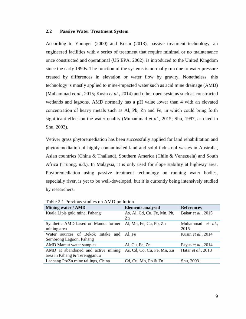
Vetiver grass phytoremediation has been successfully applied for land rehabilitation and

phytoremediation of highly contaminated land and solid industrial wastes in Australia,

Asian countries (China & Thailand), Southern America (Chile & Venezuela) and South

Africa (Truong, n.d.). In Malaysia, it is only used for slope stability at highway area.

Phytoremediation using passive treatment technology on running water bodies,

especially river, is yet to be well-developed, but it is currently being intensively studied

by researchers.

Table 2.1 Previous studies on AMD pollution

Mining water / AMD Elements analysed References

Kuala Lipis gold mine, Pahang As, Al, Cd, Cu, Fe, Mn, Pb,

Zn

Bakar et al., 2015

Synthetic AMD based on Mamut former

mining area

Al, Mn, Fe, Cu, Pb, Zn Muhammad et al.,

2015

Water sources of Bekok Intake and

Sembrong Lagoon, Pahang

Al, Fe Kusin et al., 2014

AMD Mamut water samples Al, Cu, Fe, Zn Payus et al., 2014

AMD at abandoned and active mining

area in Pahang & Terengganuu

As, Cd, Co, Cu, Fe, Mn, Zn Hatar et al., 2013

Lechang Pb/Zn mine tailings, China Cd, Cu, Mn, Pb & Zn Shu, 2003

10

2.3 Phytoremediation

Phytoremediation consists of two terminologies, whereby ‘phyto’ means plants and

‘remedium’ means to clean or keep (Sola, 2011). Phytoremediation is the application of

removing or controlling various types of pollutants from the environment with green

plants (Salt et al., 1998; Valderrama et al., 2013), in terms of water, soil or sediments. It

is classified into several respective areas such as phytoextraction, phytodegradation,

rhizofiltration, phytostabilization, and phytovolatilization. It is an effective cleanup

technology for it can removes various types of pollutants which are organic or inorganic.

Organics can be degraded or broken down in the root region or uptake by the plant,

followed by degradation, sequestration or volatilization. Inorganics cannot be broken

down but can either be neutralized or concentrated in the harvestable plant area (Pilon-

Smits, 2005).

2.3.1 Phytoextraction

Phytoextraction is the extraction of heavy metal in the soil involving translocation

process to uptake the contaminant by using plants roots (Salt et al., 1995). The root plant

is responsible to accumulate the heavy metal with the application of plant translocation.

The accumulation of heavy metal or contaminant will be removed by plant harvesting

(National Risk Management Research Laboratory, 2000). The rate of phytoextraction

depends on the root depth in soil or medium because root acts as the metal accumulator

(Kidney, 1997).

2.3.2 Phytostabilization

Phytostabilization technique is normally applicable to processes such as leaching and

soil dipersion, in order to avoid the migration or dispersion of contaminant through wind

and water erosion. The plant roots take an important role to absorb the contaminant from

the environment (NRMRL, 2000), as a result, the soluble metal ions would become

insoluble metal ions (Salt et al., 1995). This technique is very suitable for soil

contaminated with high organic matter and heavy textured soil (Cunningham et al.,

1995).

11

2.3.3 Phytodegradation (Phytotransformation)

Phytodegradation is the process in which uses the plant metabolism process, either

internal or external metabolism, by breaking down the contaminant for uptake. It is quite

different from rhizodegradation that uses microorganisms as the main medium, instead it

depends on the solubility, polarity and hydrophobicity of the medium. Thus, it can not

only be used in soil, sludge and sediment but also in groundwater and surface water

(NRMRL, 2000). Moreover, the compounds with high solubility will not be infiltrated

into the root (Schnoor et al., 1995).

The organic contaminant in the soil can be easily broken down by microbial activities,

yet it would be more effective by using plant roots – a technique known as

rhizodegradation (NRMRL, 2000). The microbial activities and population are

influenced by existence of organic acid, fatty acids, sterols, growth factor, nucleotides,

sugar, amino acid, enzymes and other compounds in the root zone. All the matter or

substances come from product of the root plant (Schnoor et al., 1995; Shrimp et al.,

1993).

2.3.4 Rhizofiltration

Rhizofiltration is the effective treatment by adsorbing contaminant contained in the

surrounding root zone in abiotic or biotic process. This application is almost similar to

phytoextraction but it is normally used on groundwater, wastewater and surface water as

hydroponic treatment; because the root can come in contact with water (NRMNL, 2000).

The process occurs during the adsorption of contaminants onto root surface or plant root

absorption. In order to carry out this treatment, the plants have to acclimatize to the

pollutants first to familiarize with the pollutants to be uptake.

2.3.5 Phytovolatization

Phytovolatization is related to phytodegradation, whereby it also absorbs contaminant

into the plant, but the contaminants will be released through the evapo-transpiration

process after modification in the plant. Hence, the contaminants will be released into the

atmosphere, whereas the groundwater or other medium would be less toxic (NRMRL,

2000).

12

Heavy metal pollution may bring forth to potential ecological risk. In contrast,

phytoremediation is a promising method for cleaning of soil and water via the pollutant

uptake by the plant (Mathe-Gaspar and Anton, 2005).

2.4 Vetiver grass (VG)

Vetiver grass (VG), scientifically known as Chrysopogon (Vetiveria) Zizanioides,

originates from India in the Graminae family. It also comes from the same grass family

which includes lemon grass, maize, sorghum, and sugarcane (Darajeh et al., 2014). VG

has been distributed throughout the equatorial and Mediterranean regions of many

countries worldwide which include all the continents of the world except Antartica

(Danh et al., 2009). VG has been used for a long time in land conservation by means of

soil and water by World Bank (Darajeh et al., 2014), but its advantages of being cheap,

effective and easy for water and soil conservation, particularly in wastewater treatment,

only emerged in the 1980s (Danh et al., 2009; Truong., 2000), due to its extraordinary

and outstanding physiological and morphological characteristics.

13

Figure 2.1 (a) Vetiver grass and its uses; (b) Vetiver grass grown hydroponically

Extensive R&D over the last 20 years in Australia, China and Thailand have found out

that VG is non-invasive species which could take up water and nutrient efficiently, and

thrives under extreme conditions in terms of soil, climate, and toxicity such as heavy

metals and agrochemicals (Truong, 2000; Truong, n.d.). Besides, Hence, VGT would be

a promising technology, in terms of economic and environment, for exploring the

treatment of running water bodies, especially river, in spite of low cost, effective, and

environmentally friendly.

VG has many distinctive characteristics which make it a suitable species for

phytoremediation of many types of pollutants such as land recovery, soil and water

management, and many more. The outstanding characteristics of VG will be discussed

below:

(a) (b)

14

2.4.1 Morphological and genetic characteristics

VG is well known for being a perennial and non-invasive grass species. It has a straight

and stiff stem in which allows it to withstand high velocity flows of water or air. For

example, Truong (2002) and Hengchaovanich (1998) have claimed that VG up to 2-m

high can survive in relatively deep-water flow (as cited in Danh et al., 2009, p. 666). As

a result, it can increase the detention time. In additional to that, it has long narrow leaves

which would produce a thick growth that will form a living barrier that cuts off and

spreads runoff water. This type of growth also allows VG to act as a potent filter by

trapping sediments and sediment-bound pollutants such as heavy metals and some

pesticide residues (Chomchalow, 2003).

Moreover, it has a complex and lacework root system, whereby it can penetrate deep

into the soil as well as in water. This extensive root system can reduce and prohibit deep

drainage, enhance bed stability of the soil and nutrient uptake. Hengchaovanich (1998)

asserts that the root system can grow up to 3 – 4 metres in a year (as cited in Danh et al.,

2009, p. 666 & Truong, 2000, p. 47). Furthermore, this dense and finely structured root

system could create an environment ideal for microbiological processes in the

rhizosphere.

A distinctive characteristic of VG is that it tends to grow into a thick hedge when closely

planted together. As VG loves to grow upright then extending laterally, it is good to

plant on farms with minimal changes to its existing layout. Not only that, its non-

invasive feature ensures that there is no competition with adjacent plants for survival.

Due to these characteristics, VG is often used as slope stability by river banks and

highways to prevent erosion.

15

2.4.2 Physiological characteristics

VG can adapt extreme climatic and weather conditions such as drought, flood, frost, heat

wave and inundation (Chomchalow, 2003). In fact, Truong (1999a) has claimed that VG

can survive up to 6 months in drought. It is able to tolerate flood and areas where with

too much water, for instance submergence for more than 120 days (Xia et al., 2003),

making it perfect for wetlands for it can consume high amount of water.

Although VG is a perennial and tropical grass, it can tolerate and survive under extreme

temperature ranging from -15°C to 55°C, which means it can survive in extreme cold

and hot climatic condition. A study by Dudai (2006) has also claimed that VG can be

used in Mediterranean conditions. VG growth is limited by frost, in which the shoot died

but the root survived (Danh et al., 2009).

VG has high tolerance and adaptability to extreme edaphic conditions such as soil with

high acidity and alkalinity. It can thrive under a wide pH range and adapt to saline, sodic

and magnesic conditions, and aluminium and manganese toxicities (Chomchalow, 2003;

Truong and Baker, 1998 and 1997, as cited in Danh et al., 2009). VG can survive

between pH 3.3 to 9.5 at nutrient-adequate condition and saline soil with high electrical

conductivity up to 4.0 (Danh et al., 2009; Webb, 2009).

Another unique characteristics of VG is that it has high tolerance to elevated

concentrations of heavy metals such as As, Cd, Cu, Cr, Pb, Hg, Ni, Se and Zn in the soil

(Danh et al., 2009: Chomchalow, 2003; Shu, 2003). Furthermore, it has great potential

in dissolved nutrient uptake and other organic constituents, especially N and P, and BOD

and COD respectively (Darajeh et al., 2014; Shu, 2003; Xia et al., 2000; Pinthong et al.,

1998 as cited in Truong, 2000, p. 47). Another finding about VG is its high resistance

towards herbicide and pesticide (Chomchalow, 2003; West et al., 1996 as cited in

Truong, 2000, p. 47).

16

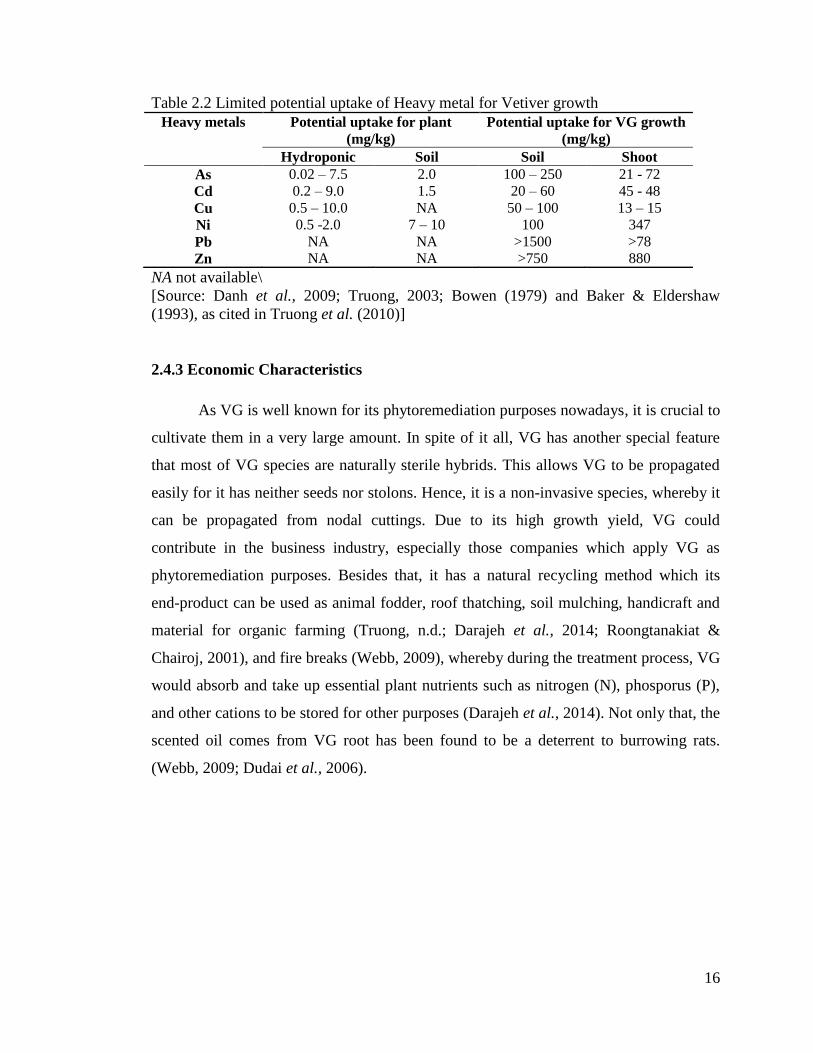
Table 2.2 Limited potential uptake of Heavy metal for Vetiver growth

Heavy metals Potential uptake for plant

(mg/kg)

Potential uptake for VG growth

(mg/kg)

Hydroponic Soil Soil Shoot

As 0.02 – 7.5 2.0 100 – 250 21 - 72

Cd 0.2 – 9.0 1.5 20 – 60 45 - 48

Cu 0.5 – 10.0 NA 50 – 100 13 – 15

Ni 0.5 -2.0 7 – 10 100 347

Pb NA NA >1500 >78

Zn NA NA >750 880

NA not available\

[Source: Danh et al., 2009; Truong, 2003; Bowen (1979) and Baker & Eldershaw

(1993), as cited in Truong et al. (2010)]

2.4.3 Economic Characteristics

As VG is well known for its phytoremediation purposes nowadays, it is crucial to

cultivate them in a very large amount. In spite of it all, VG has another special feature

that most of VG species are naturally sterile hybrids. This allows VG to be propagated

easily for it has neither seeds nor stolons. Hence, it is a non-invasive species, whereby it

can be propagated from nodal cuttings. Due to its high growth yield, VG could

contribute in the business industry, especially those companies which apply VG as

phytoremediation purposes. Besides that, it has a natural recycling method which its

end-product can be used as animal fodder, roof thatching, soil mulching, handicraft and

material for organic farming (Truong, n.d.; Darajeh et al., 2014; Roongtanakiat &

Chairoj, 2001), and fire breaks (Webb, 2009), whereby during the treatment process, VG

would absorb and take up essential plant nutrients such as nitrogen (N), phosporus (P),

and other cations to be stored for other purposes (Darajeh et al., 2014). Not only that, the

scented oil comes from VG root has been found to be a deterrent to burrowing rats.

(Webb, 2009; Dudai et al., 2006).

17

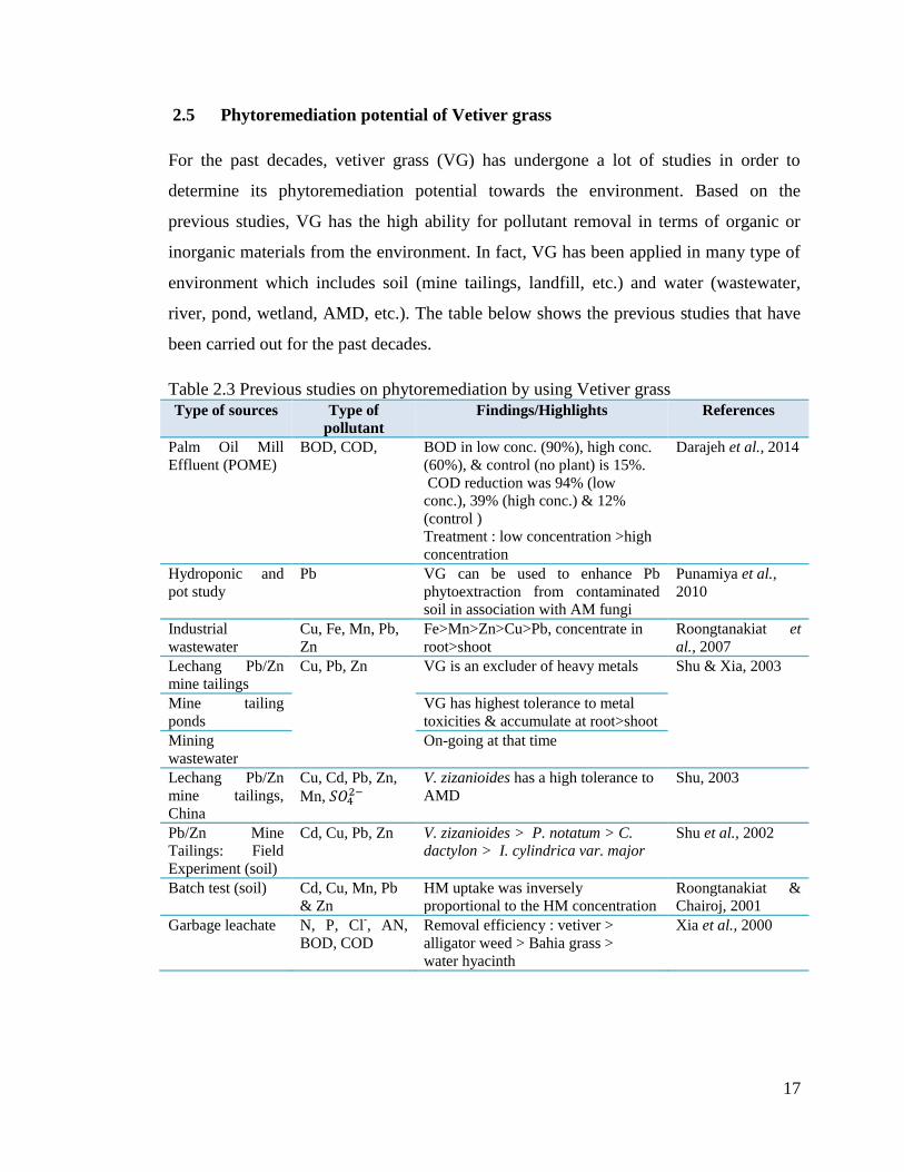
2.5 Phytoremediation potential of Vetiver grass

For the past decades, vetiver grass (VG) has undergone a lot of studies in order to

determine its phytoremediation potential towards the environment. Based on the

previous studies, VG has the high ability for pollutant removal in terms of organic or

inorganic materials from the environment. In fact, VG has been applied in many type of

environment which includes soil (mine tailings, landfill, etc.) and water (wastewater,

river, pond, wetland, AMD, etc.). The table below shows the previous studies that have

been carried out for the past decades.

Table 2.3 Previous studies on phytoremediation by using Vetiver grass

Type of sources Type of

pollutant

Findings/Highlights References

Palm Oil Mill

Effluent (POME)

BOD, COD, BOD in low conc. (90%), high conc.

(60%), & control (no plant) is 15%.

COD reduction was 94% (low

conc.), 39% (high conc.) & 12%

(control )

Treatment : low concentration >high

concentration

Darajeh et al., 2014

Hydroponic and

pot study

Pb VG can be used to enhance Pb

phytoextraction from contaminated

soil in association with AM fungi

Punamiya et al.,

2010

Industrial

wastewater

Cu, Fe, Mn, Pb,

Zn

Fe>Mn>Zn>Cu>Pb, concentrate in

root>shoot

Roongtanakiat et

al., 2007

Lechang Pb/Zn

mine tailings

Cu, Pb, Zn VG is an excluder of heavy metals Shu & Xia, 2003

Mine tailing

ponds

VG has highest tolerance to metal

toxicities & accumulate at root>shoot

Mining

wastewater

On-going at that time

Lechang Pb/Zn

mine tailings,

China

Cu, Cd, Pb, Zn,

Mn, 𝑆𝑂42−

V. zizanioides has a high tolerance to

AMD

Shu, 2003

Pb/Zn Mine

Tailings: Field

Experiment (soil)

Cd, Cu, Pb, Zn V. zizanioides > P. notatum > C. dactylon > I. cylindrica var. major

Shu et al., 2002

Batch test (soil) Cd, Cu, Mn, Pb

& Zn

HM uptake was inversely

proportional to the HM concentration

Roongtanakiat &

Chairoj, 2001

Garbage leachate N, P, Cl-, AN,

BOD, COD

Removal efficiency : vetiver >

alligator weed > Bahia grass >

water hyacinth

Xia et al., 2000

18

2.6 Other plant species for phytoremediation

Apart from vetiver grass, Jiji grass (Achnatherum splendens), a perennial grass in north

China, is noted to have similar characteristics to vetiver. However, it is extremely

drought and cold tolerant although it has a less dense and weaker leaf system (Xu,

2002). According to Xia et al. (2003), Bermuda grass also has high tolerance towards

submergence but it is native to Africa and widely spread throughout the southwest and

southern United States, which is not common in Malaysia. Moreover, there are many

different plant species that are used for phytoremediation like bahia grass (Paspalum

notatum Flugge), Bulrush (Typha), Common Reed (Phragmites Australis), Water

Hyacinth (Eichhornia crassipes), and Water Lettuce (Pistia stratiotes L.), other than

Vetiver Grass (Chrysopogon zizanioides) and for the treatment of water, and it turned

out that water hyacinth, water lettuce and VG were selected for review due to their

efficiency of HM removal and other pollutants with high biomass yield and adaptability

of ecological factors (Gupta et al., 2012). These three plants have their distinct pollutant

removal capabilities depending on both abiotic or biotic environmental factors, level of

contamination, and others. In short, VG is used in this study in order to increase the

knowledge of VG technology in treating river water.

19

Table 2.4 Previous studies of other plant species for phytoremediation of water

Type of water Species Uptake of HM References

Ctalamochita river

water

Potamogeton pusillus L.

Myriophyllum aquaticum

(Vell.) Verdc.

Co, Cu, Fe, Mn, Ni, Pb

& Zn

Harguinteguy et al.,

2015

Composting

wastewater

Eichhornia crassipes Cd, Cr, Cu, Fe, Mn, Ni,

Pb, Zn

Rezania et al., 2015

Swartkops Estuary Phragmites australis

Typha capensis

Spartina maritima

Cd, Cu, Pb, Zn Phillips et al., 2015

Highway stormwater

ponds

Carex riparia

Juncus effusus

Cd, Ni, Zn Ladislas et al., 2015

Watercourses of

Egypt

Myriophyllum spicatum L Mn>Fe>Zn>Cu>Ni>Pb>

Cd

Galal & Shehata,

2014

Synthetic water

(Batch study)

Eichhornia Crassipes Cd & Cu Swain et al., 2014

Urban stormwater

runoff

Carex riparia

Juncus effusus

Cd, Ni, Zn Ladislas et al., 2013

Gold mine wastewater Cabomba piauhyensis,

Egeria densa

Hydrilla verticillata

As, Zn, Al Bakar et al., 2013

Ex - tin mining

catchment

Cyperus rotundus L.

Imperata cylindrica

Lycopodium cernuum,

Melastoma

malabathricum,

Mimosa pudica Linn,

Nelumbo nucifera,

Phragmites australis L.,

Pteris vittata L.

Salvinia molesta

As, Cu, Pb, Sn, Zn Ashraf et al., 2011;

Ashraf et al., 2013

Synthetic wáter Pistia stratiotes Co, Cr Prajapati et al.,

2012

Synthetic water Phylidrum lanuginosum Cu, Pb, Zn Hanidza et al., 2011

Metal-contaminated

coastal water

Eichornia crassipes As, Cd, Cu, Cr, Fe, Mn,

Ni, Pb, V and Zn

Agunbiade et al.,

2009

Mine tailing ponds

Mining wastewater

AMD

Rumex acetosa

Z. mays

Alocasia macrorrhiza

Chrysopogon aciculatus

Cyperus alternifolius

Gynura crepidiodes

Panicum repens

Phragmites australis

Cu, Pb, Zn

Cd. Cu, Pb, Zn

Cd, Cu, Mn, Pb, Zn

Shu & Xia, 2003

20

2.7 Heavy metal

Heavy metals are found everywhere in the environment, whereby it could be contributed

by natural state (water, air and soil) or anthropogenic activities (surface water, waste,

soils, etc.). As a result from the technology development and improvement, they are

widely used in the industries such as the application in metal processing, electroplating,

electronics and chemical processing (Fingerman & Nagabushanam, 2005).

Environmental pollution contributed by toxic heavy metals has becoming such a concern

worldwide. This is because it would bring forth adverse effects to the environment,

especially agricultural industries in terms of crop yields, biomass and soil fertility, in

return it would lead to accumulation and bio-magnification process to occur in the food

chain. Due to their persistence, toxicity and ubiquitousness in the environment, heavy

metals are of particular interest in stormwater runoff (Ladislas et al., 2013). The effects

of heavy metals are undesirable, even in a minute quantity. The toxic effects can be

detected in human and animals after a long period of time (Srivastav et al., 1993). The

list of heavy metal concentration is tabulated in the Appendix 1.

2.7.1 Copper (Cu)

Copper (Cu) can be naturally found in the environment, however the concentration of

Cu in the environment has been rapidly increased due to anthropogenic activities. Some

of the natural sources of Cu are such as decaying vegetation, sea spray, and forest fire.

On the other hand, the Cu-releasing human activities include activities like mining,

wood manufacturing, electric and electronic manufacturing, phosphate fertilizer

manufacturing, metal manufacturing, and many others. Cu is one of the minerals

required by humans as well as plants. Cu is responsible for energy production during

biochemical reaction in human. Not only that, it can transform melanin, which is good

for the heart and arteries to maintain and repair connective tissues. However, over-

nutrition of Cu can be a problem to living things, which is known as trace element –

element that could pose harm to living things even though the concentration is very low.

Cu is commonly found in food and water, instead of air because it has low concentration

in the atmosphere.

21

2.7.2 Iron (Fe)

Iron (Fe) is one of the major mineral required in the human and plants. In human, it is

crucial as it can be found in every cells in the body, most importantly is that it associates

with the red blood cells – oxygen carrier. Malnutrition of Fe would cause body

weakness, but excess nutrition of Fe can cause adverse health effect instead. Basically,

Fe is highly demanded by the development of any aerobic life on Earth due to its

necessity in most biological system but it can be a toxic if over-nutrition.

2.7.3 Lead (Pb)

Lead (Pb) can be found naturally in the Earth’s crust in terms of bluish-grey metal. It

contains in the environment at a minute quantity. Since it is a toxic substance even at

relatively low concentration, people are concerned about the health. Lead can enter into

human body via inhalation and ingestion, but mostly via oral ingestion. It tends to bio-

accumulate in the blood stream. Lead poisoning is the most vulnerable symptoms of

excessive intake of Pb for it can be fatal to human up to certain extent, especially

children. Pb can associate with other toxic elements at a relatively low level, especially

Cd and Hg, in terms of synergistic toxicity.

2.7.4 Manganese (Mn)

Manganese (Mn) occurs naturally not only in the environment (rocks) but also in foods,

in which it could be either natural or synthetic form. Mn is one of the trace elements

which is essential for good health. There are several types of food that consists of Mn,

such as whole grains, beans, cereals and tea. Therefore, Mn normally enters the body via

ingestion. Mn is important to human because it would maintain healthy bone structure

and metabolism, and it aids in production of collagen which maintains skin health.

2.7.5 Zinc (Zn)

Zinc (Zn) is an essential trace mineral for living organisms, especially human because it

exists in most cells for human metabolism. Zn is found in all medium on Earth – air,

water, and soil. Sphalente (ZnS) is often found on Earth’s surface and underground. In

fact, Zn is mostly found in water due to deposition into sediment, in which it binds with

22

inorganic and organic matter. The importance of Zn is immune system, growth, vision,

taste, smell, and reproduction.

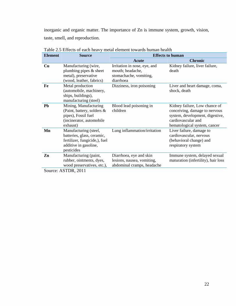
Table 2.5 Effects of each heavy metal element towards human health

Element Source Effects to human

Acute Chronic

Cu Manufacturing (wire,

plumbing pipes & sheet

metal), preservative

(wood, leather, fabrics)

Irritation in nose, eye, and

mouth; headache,

stomachache, vomiting,

diarrhoea

Kidney failure, liver failure,

death

Fe Metal production

(automobile, machinery,

ships, buildings),

manufacturing (steel)

Dizziness, iron poisoning Liver and heart damage, coma,

shock, death

Pb Mining, Manufacturing

(Paint, battery, solders &

pipes), Fossil fuel

(incinerator, automobile

exhaust)

Blood lead poisoning in

children

Kidney failure, Low chance of

conceiving, damage to nervous

system, development, digestive,

cardiovascular and

hematological system, cancer

Mn Manufacturing (steel,

batteries, glass, ceramic,

fertilizer, fungicide,), fuel

additive in gasoline,

pesticides

Lung inflammation/irritation Liver failure, damage to

cardiovascular, nervous

(behavioral change) and

respiratory system

Zn Manufacturing (paint,

rubber, ointments, dyes,

wood preservatives, etc.),

Diarrhoea, eye and skin

lesions, nausea, vomiting,

abdominal cramps, headache

Immune system, delayed sexual

maturation (infertility), hair loss

Source: ASTDR, 2011

23

2.8 Nutrients essential for plant growth

The nutrients essential for plant growth are classified into two categories which are

macronutrients and micronutrients. Macronutrients are the most important class of

nutrients as it requires a relatively large amount for the plant growth. On the other hand,

micronutrients are required only a small amount in which they are used in aid of the

plant growth. As Weast (1984) asserts, “there are 17 heavy metals indicated to be bio-

available for living cells and importance for organism and ecosystems based on the

solubility under the physiological condition (as cited in Kamaruzaman, 2011, p.16).

Among these heavy metals, Fe, Mo, Mn and Cu are some important micronutrients in

order to carry out normal physiological regulatory functions for plants. Meanwhile, Zn,

Ni, Cu, V, Co, Pb and Cr are trace elements that could be toxic to plants at certain toxic

level. As Mengel and Kirkby (2001) asserts, the cell organelle which is most sensitive to

Mn deficiency is chloroplast, a plant organelle responsible for photosynthesis process

(McCauley, 2011, p. 12). The amount of nutrients absorbed by the plant depends on the

plant function, plant mobility and plant deficiency (Khalil, 2011). Table 2.8a shows the

essential nutrients required for plant growth, while Table 2.8b shows overall symptoms

of malnutrition or over-nutrition.

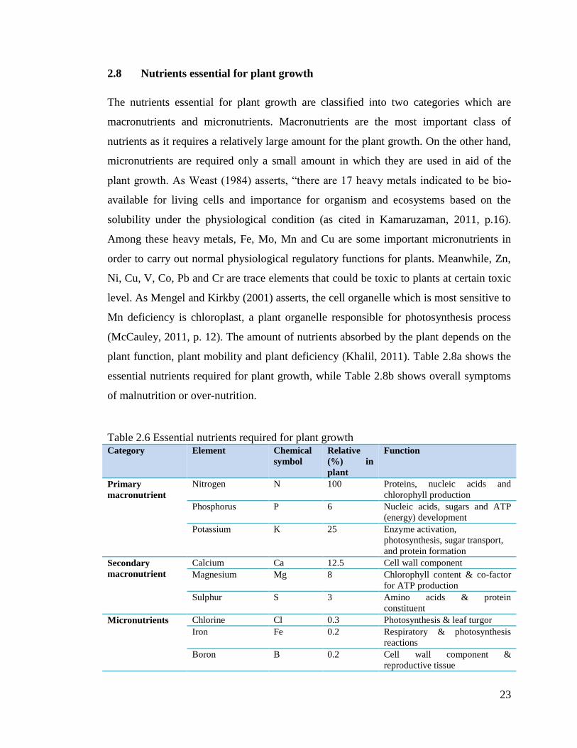
Table 2.6 Essential nutrients required for plant growth Category Element Chemical

symbol

Relative

(%) in

plant

Function

Primary

macronutrient

Nitrogen N 100 Proteins, nucleic acids and

chlorophyll production

Phosphorus P 6 Nucleic acids, sugars and ATP

(energy) development

Potassium K 25 Enzyme activation,

photosynthesis, sugar transport,

and protein formation

Secondary

macronutrient

Calcium Ca 12.5 Cell wall component

Magnesium Mg 8 Chlorophyll content & co-factor

for ATP production

Sulphur S 3 Amino acids & protein

constituent

Micronutrients Chlorine Cl 0.3 Photosynthesis & leaf turgor

Iron Fe 0.2 Respiratory & photosynthesis

reactions

Boron B 0.2 Cell wall component &

reproductive tissue

24

Manganese Mn 0.1 Enzyme activation for

photosynthesis

Zinc Zn 0.03 Growth hormone production &

internode elongation (Enzyme

activation)

Copper Cu 0.01 Enzyme component(chlorophyll

production, respiration and

protein synthesis)

Molybdenum Mo 0.0001 Nitrogen fixation process

Sources: McCauley (2011); Bennett (1993), as cited in Khalil (2011)

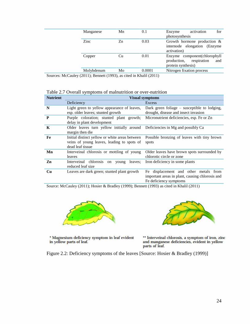
Table 2.7 Overall symptoms of malnutrition or over-nutrition Nutrient Visual symptoms

Deficiency Excess

N Light green to yellow appearance of leaves,

esp. older leaves; stunted growth

Dark green foliage – susceptible to lodging,

drought, disease and insect invasion

P Purple coloration; stunted plant growth;

delay in plant development

Micronutrient deficiencies, esp. Fe or Zn

K Older leaves turn yellow initially around

margin then die

Deficiencies in Mg and possibly Ca

Fe Initial distinct yellow or white areas between

veins of young leaves, leading to spots of

dead leaf tissue

Possible bronzing of leaves with tiny brown

spots

Mn Interveinal chlorosis or mottling of young

leaves

Older leaves have brown spots surrounded by

chlorotic circle or zone

Zn Interveinal chlorosis on young leaves;

reduced leaf size

Iron deficiency in some plants

Cu Leaves are dark green; stunted plant growth Fe displacement and other metals from

important areas in plant, causing chlorosis and

Fe deficiency symptoms

Source: McCauley (2011); Hosier & Bradley (1999); Bennett (1993) as cited in Khalil (2011)

Figure 2.2: Deficiency symptoms of the leaves [Source: Hosier & Bradley (1999)]

25

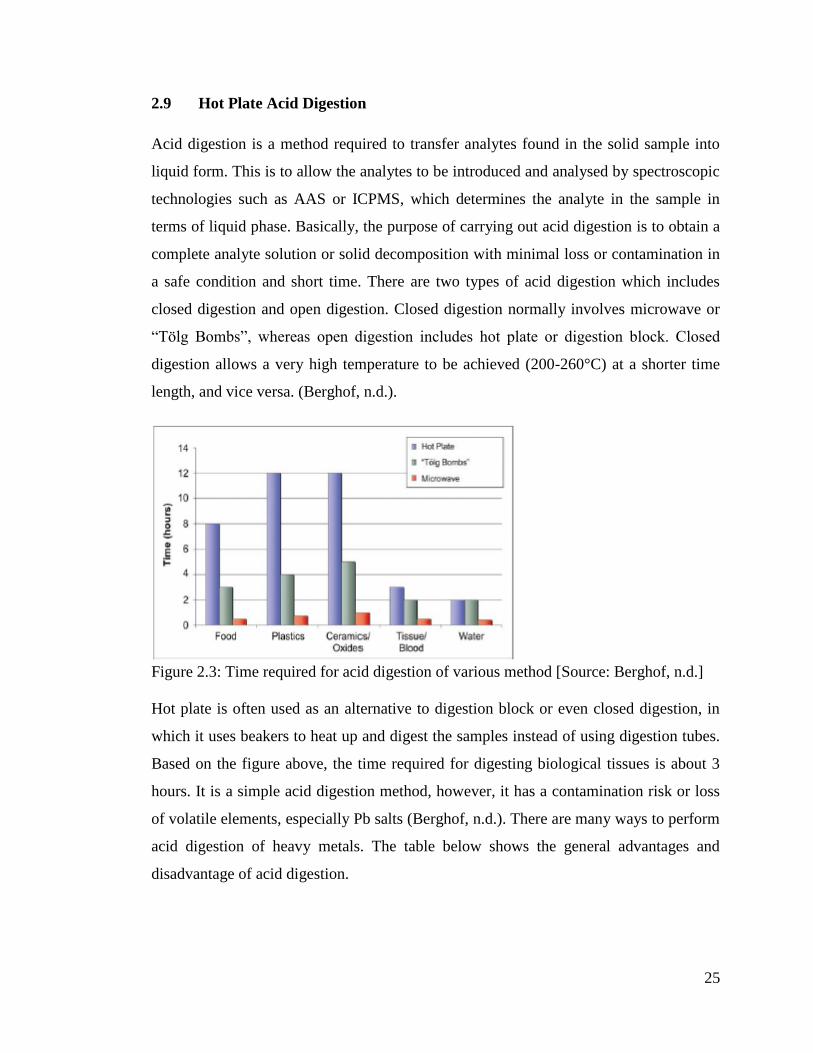
2.9 Hot Plate Acid Digestion

Acid digestion is a method required to transfer analytes found in the solid sample into

liquid form. This is to allow the analytes to be introduced and analysed by spectroscopic

technologies such as AAS or ICPMS, which determines the analyte in the sample in

terms of liquid phase. Basically, the purpose of carrying out acid digestion is to obtain a

complete analyte solution or solid decomposition with minimal loss or contamination in

a safe condition and short time. There are two types of acid digestion which includes

closed digestion and open digestion. Closed digestion normally involves microwave or

“Tölg Bombs”, whereas open digestion includes hot plate or digestion block. Closed

digestion allows a very high temperature to be achieved (200-260°C) at a shorter time

length, and vice versa. (Berghof, n.d.).

Figure 2.3: Time required for acid digestion of various method [Source: Berghof, n.d.]

Hot plate is often used as an alternative to digestion block or even closed digestion, in

which it uses beakers to heat up and digest the samples instead of using digestion tubes.

Based on the figure above, the time required for digesting biological tissues is about 3

hours. It is a simple acid digestion method, however, it has a contamination risk or loss

of volatile elements, especially Pb salts (Berghof, n.d.). There are many ways to perform

acid digestion of heavy metals. The table below shows the general advantages and

disadvantage of acid digestion.

26

Table 2.8 Pros and cons of acid digestion method

Acid digestion method Advantages Disadvantages

Hydrofluoric acid-perchloric

acid (HF-HClO4) digestion

Most effective extraction

Capable of measuring

metals associated with

silicates

Acids used are extremely

dangerous

Nitric acid (HNO3) digestion Measure all metals, except

those bounded with

silicates

Less effective than HF-

HClO4 digestion

Aqua regia digestion Safer than HF-HClO4

digestion

Longer digestion time

required

Nitric acid - hydrogen

peroxide (HNO3-H2O2)

digestion

Reasonable measurement

of metals in samples

Does not measure true

total metal concentration

Analytes may loss due to

evaporation

The method of digesting plant samples in concentrated HNO3, with or without H2O2,

has been well established and widely used for determination of HM concentrations in

plant samples (Huang, 1985, as cited in Huang et al., 2004, p. 428). Zheljazkov and

Warman (2002) claimed that HNO3 and HNO3-HClO4 provided similar levels and good

recoveries of Cd and Pb (as cited in Hseu, 2004, p. 54). Moreover, nitric acid procedure

has the highest recoveries of Cd, Mn and Ni of compost samples (Hseu, 2004).

Perchloric acid is also advised not to be used for acid digestion due to its risk and

problem of KClO4 precipitation. Overnight HNO3 digestion and HNO3-H2O2 digestion

of reed plants have high recoveries of Cd, Cu, Pb, Zn, Fe and Mn (Laing et al., 2003),

however, it all depends on the type of plants as well. There are several studies that use

HNO3 destruction of plant tissues for heavy metal analysis (Phillips et al., 2015;

Punamiya et al., 2010; Ippolito & Barbarick, 2000; Havlin & Soltanpour, 1980). H2O2 is

avoided to be used in this research in order to prevent the loss of analytes, rather than

undigested. According to Sastre et al. (2002), nitric acid digestion can be used for

samples with high organic matter content such as plant material and organic soil as most

of the RSD values were lower than 5%. Moreover, the amount of sample used in this

experiment is also very small, which is 0.1g. Hence, it is assumed that this method is

27

enough to digest the small amount of sample, whereby the sample is also grinded into

very fine powder form.

2.10 Flame Atomic Absorption Spectrometry (F-AAS)

Atomic absorption spectrometry (AAS) is a spectrometric technology that is used to

determine inorganic element found in the environmental samples by means of liquid

form. There are several types of flame spectrometry which includes F-AAS, FES and

Atomic Fluorescent Spectroscopy. The principle of F-AAS is the optical radiation

(light) absorption, based on the electromagnetic spectrum of each element (190 – 850

nm), by free atoms into gaseous state, in which the sample is aspirated into a flame and

then atomized via a nebulizer due to Venturi effect. Venturi effect is a result of collision

from high speed gas with the liquid samples injected into the nebulizer, whereby the

liquid would turn into small drops and eventually into aerosol. The flame used normally

consists of air and acetylene. It will direct the light beam into a monochromator to

measure the concentration of element by using a detector. Each element has its own

wavelength for this process to occur, hence only an element can be detected at a time.

28

CHAPTER 3

METHODOLOGY

3.1 Method Summary

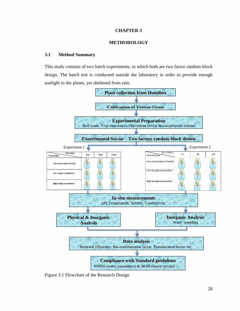
This study consists of two batch experiments, in which both are two factor random block

design. The batch test is conducted outside the laboratory in order to provide enough

sunlight to the plants, yet sheltered from rain.

Figure 3.1 Flowchart of the Research Design

Cultivation of Vetiver Grass

In-situ measurements pH, Temperature, Salinity, Conductivity

Data analysis

Removal efficiency, Bio-concentration factor, Translocation factor, etc.

Compliance with Standard guidelines

NWQS (water parameters) & MOH (heavy metals)

Plant collection from Humibox

Experimental Set-up – Two factors random block design

Experiment 1 Experiment 2

Experimental Preparation Acid wash, Trial experiment (Harvesting period &concentration setting)

Inorganic Analysis Water sampling

Physical & Inorganic

Analysis Water and plant sampling

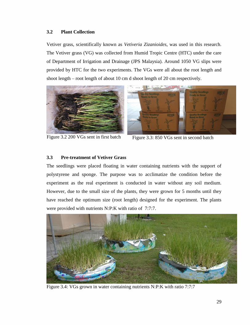
29

3.2 Plant Collection

Vetiver grass, scientifically known as Vetiveria Zizanioides, was used in this research.

The Vetiver grass (VG) was collected from Humid Tropic Centre (HTC) under the care

of Department of Irrigation and Drainage (JPS Malaysia). Around 1050 VG slips were

provided by HTC for the two experiments. The VGs were all about the root length and

shoot length – root length of about 10 cm d shoot length of 20 cm respectively.

3.3 Pre-treatment of Vetiver Grass

The seedlings were placed floating in water containing nutrients with the support of

polystyrene and sponge. The purpose was to acclimatize the condition before the

experiment as the real experiment is conducted in water without any soil medium.

However, due to the small size of the plants, they were grown for 5 months until they

have reached the optimum size (root length) designed for the experiment. The plants

were provided with nutrients N:P:K with ratio of 7:7:7.

Figure 3.4: VGs grown in water containing nutrients N:P:K with ratio 7:7:7

Figure 3.2 200 VGs sent in first batch Figure 3.3: 850 VGs sent in second batch

30

3.3.1 Trial experiment

The trial experiment was carried out to evaluate the heavy metal uptake by Vetiver grass

in two planting densities within a range of heavy metal concentrations. The purpose is to

prepare for the big scale experiment so that we could know when to harvest the plants,

how many tillers should be used, and which concentration can be set as the low and high

strength concentration. In other words, the optimization of the experiment for heavy

metal uptake from the water was the main study of this experiment in order to comply

with the plant harvesting in the real experiment. The experiment is set up as shown in

Figure 3.5, whereby there are two treatments of 4 tillers and 10 tillers exposed to heavy

metal concentration of 0.5ppm, 1.0ppm, 2.0ppm, 4.0ppm, 8.0ppm and 10ppm

respectively. All the slips were trimmed to a height of 25-cm and root length of 15-cm.

The water sample at 0-hour contact time was taken to indicate the initial heavy metal

concentration in the synthetic water. The physical parameters such as pH, temperature,

salinity and electrical conductivity (EC) were measured daily. 15-mL of water samples

were taken at each sampling and filtered through 0.45-μm cellulose acetate filter paper.

The samples were then preserved to pH<2 prior to AAS analysis (Appelo and Postma,

1993). The growth and toxicity symptoms were also observed.

Figure 3.5: Treatment of control and each plant with 4 tillers and 10 tillers respectively

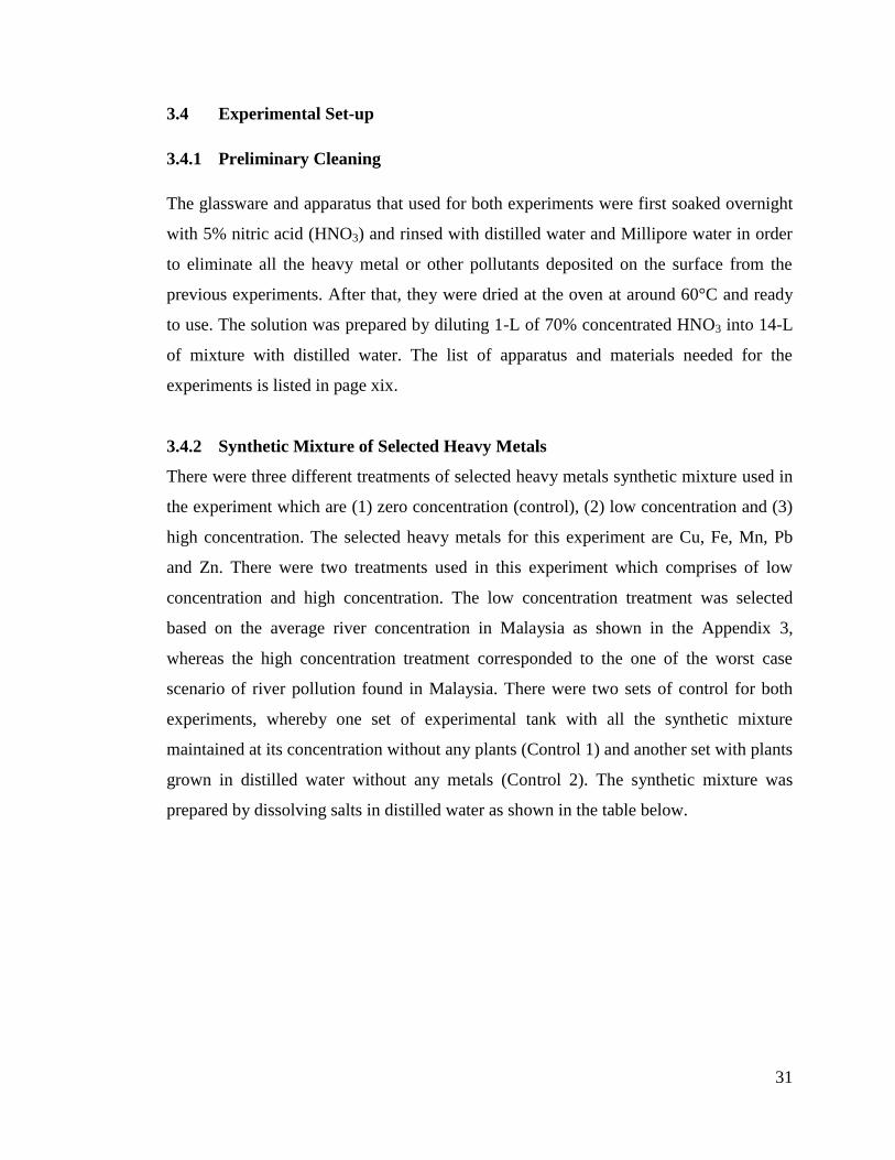
31

3.4 Experimental Set-up

3.4.1 Preliminary Cleaning

The glassware and apparatus that used for both experiments were first soaked overnight

with 5% nitric acid (HNO3) and rinsed with distilled water and Millipore water in order

to eliminate all the heavy metal or other pollutants deposited on the surface from the

previous experiments. After that, they were dried at the oven at around 60°C and ready

to use. The solution was prepared by diluting 1-L of 70% concentrated HNO3 into 14-L

of mixture with distilled water. The list of apparatus and materials needed for the

experiments is listed in page xix.

3.4.2 Synthetic Mixture of Selected Heavy Metals

There were three different treatments of selected heavy metals synthetic mixture used in

the experiment which are (1) zero concentration (control), (2) low concentration and (3)

high concentration. The selected heavy metals for this experiment are Cu, Fe, Mn, Pb

and Zn. There were two treatments used in this experiment which comprises of low

concentration and high concentration. The low concentration treatment was selected

based on the average river concentration in Malaysia as shown in the Appendix 3,

whereas the high concentration treatment corresponded to the one of the worst case

scenario of river pollution found in Malaysia. There were two sets of control for both

experiments, whereby one set of experimental tank with all the synthetic mixture

maintained at its concentration without any plants (Control 1) and another set with plants

grown in distilled water without any metals (Control 2). The synthetic mixture was

prepared by dissolving salts in distilled water as shown in the table below.

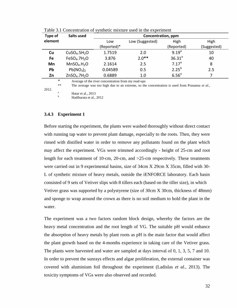
32

Table 3.1 Concentration of synthetic mixture used in the experiment

Type of element

Salts used Concentration, ppm

Low (Reported)*

Low (Suggested) High (Reported)

High (Suggested)

Cu CuSO4.5H2O 1.7519 2.0 9.19a 10 Fe FeSO4.7H2O 3.876 2.0** 36.31a 40 Mn MnSO4.H2O 2.1614 2.5 7.17a 8 Pb Pb(NO3)2 0.04589 0.5 2.25b 2.5 Zn ZnSO4.7H2O 0.6889 1.0 6.56a 7

* Average of the river concentration from my read-ups

** The average was too high due to an extreme, so the concentration is used from Prasanna et al.,

2012.

a Hatar et al., 2013

b Hadibarata et al., 2012

3.4.3 Experiment 1

Before starting the experiment, the plants were washed thoroughly without direct contact

with running tap water to prevent plant damage, especially to the roots. Then, they were

rinsed with distilled water in order to remove any pollutants found on the plant which

may affect the experiment. VGs were trimmed accordingly - height of 25-cm and root

length for each treatment of 10-cm, 20-cm, and >25-cm respectively. These treatments

were carried out in 9 experimental basins, size of 34cm X 29cm X 35cm, filled with 30-

L of synthetic mixture of heavy metals, outside the iENFORCE laboratory. Each basin

consisted of 9 sets of Vetiver slips with 8 tillers each (based on the tiller size), in which

Vetiver grass was supported by a polystyrene (size of 30cm X 30cm, thickness of 48mm)

and sponge to wrap around the crown as there is no soil medium to hold the plant in the

water.

The experiment was a two factors random block design, whereby the factors are the

heavy metal concentration and the root length of VG. The suitable pH would enhance

the absorption of heavy metals by plant roots as pH is the main factor that would affect

the plant growth based on the 4-months experience in taking care of the Vetiver grass.

The plants were harvested and water are sampled at days interval of 0, 1, 3, 5, 7 and 10.

In order to prevent the sunrays effects and algae proliferation, the external container was

covered with aluminium foil throughout the experiment (Ladislas et al., 2013). The

toxicity symptoms of VGs were also observed and recorded.

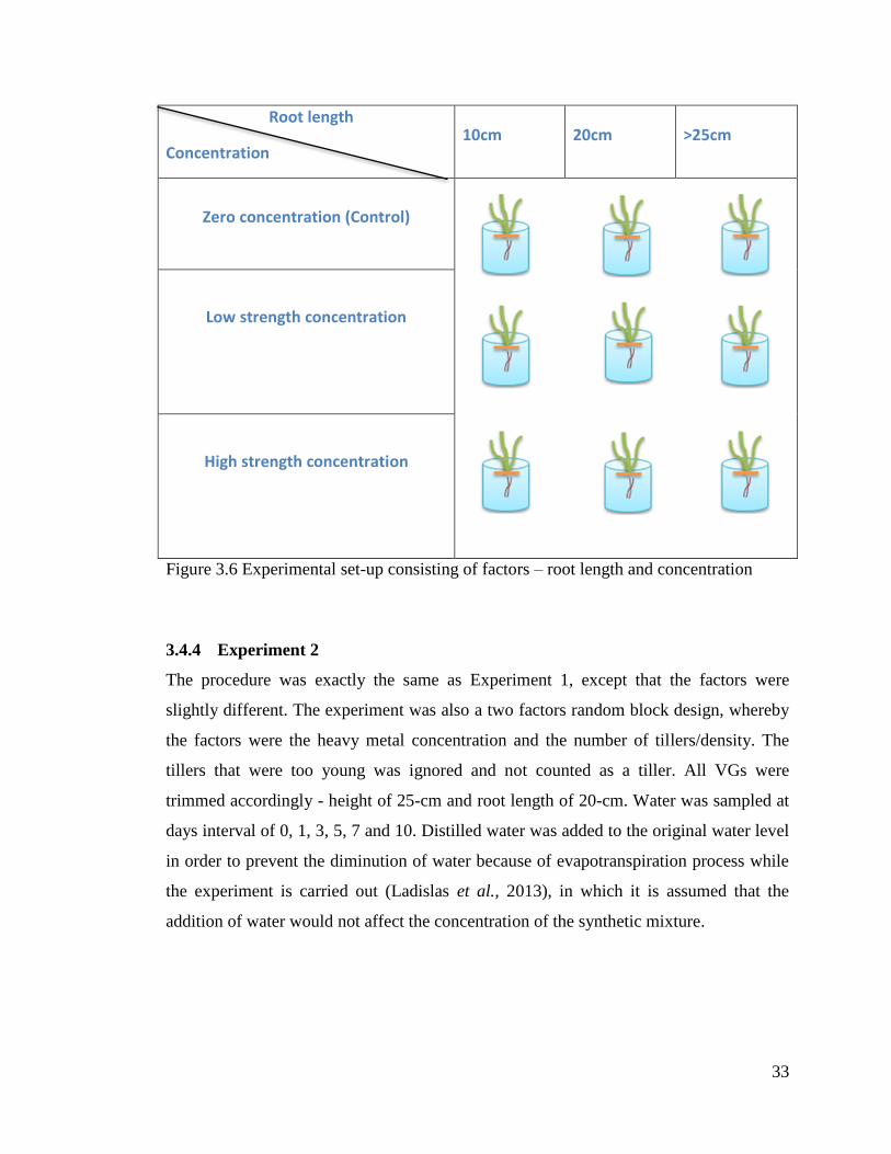
33

Figure 3.6 Experimental set-up consisting of factors – root length and concentration

3.4.4 Experiment 2

The procedure was exactly the same as Experiment 1, except that the factors were

slightly different. The experiment was also a two factors random block design, whereby

the factors were the heavy metal concentration and the number of tillers/density. The

tillers that were too young was ignored and not counted as a tiller. All VGs were

trimmed accordingly - height of 25-cm and root length of 20-cm. Water was sampled at

days interval of 0, 1, 3, 5, 7 and 10. Distilled water was added to the original water level

in order to prevent the diminution of water because of evapotranspiration process while

the experiment is carried out (Ladislas et al., 2013), in which it is assumed that the

addition of water would not affect the concentration of the synthetic mixture.

Root length

Concentration 10cm 20cm >25cm

Zero concentration (Control)

Low strength concentration

High strength concentration

34

Figure 3.7 Experimental Set-up consisting of factors – tiller density and concentration

3.4.5 Setting up Experiment 1 and 2

The real experiment was being set-up outside the ENFORCE lab. The plants were

chosen carefully based on the experimental requirement and transferred to new

polystyrene. Meanwhile, they were allowed to acclimatize once again for a few days

before the experiment as the transferring might affect some of the roots.

Figure 3.8 Experimental set-up in preparation for Experiment 1 and Experiment 2

respectively (Day 0); and the plant acclimatization of selected plants prior to the

experiment

No. of tillers

Concentration 25 50 100

Zero concentration (Control)

Low strength concentration

High strength concentration

35

3.5 Laboratory analysis

3.5.1 Water sampling

The water sampling was done at each time frame accordingly for both experiments.

There were two parameters involved in this study which are in-situ and ex-situ. The in-

situ parameters were such as pH, temperature, electrical conductivity (EC), and salinity.

On the other hand, the ex-situ parameter was the analysis of selected heavy metals in the

synthetic mixture.

50-mL of water sample was obtained in a centrifuge tube and brought immediately to

the laboratory. The water samples were filtered by using 0.45µm cellulose acetate filter

paper in order to remove large biological materials, which could cause interference by

reacting with the analyte during storage as well as the pre-requirement to be run by AAS.

The water samples were then acidified to pH<2 by addition of 0.7-ml HNO3 Suprapur 65%

(Appelo and Postma, 1993) in order to preserve most elements by reducing precipitation

and adsorption losses to container walls as well as to prohibit microbial activity.

3.5.2 Plant harvesting

Each plant was harvested from each treatment for the respective time frame for

Experiment 1. The plants were rinsed with tap water followed by distilled water in order

to wash off any dust or dirt deposited on the shoots and residual HM on the root surface.

The wet weight of each sample was weighed using analytical balance and recorded in a

sampling record sheet. Plants biomass was separated in two samples which consist of

shoots and roots. The VG root crowns were not harvested due to the assumption for its

inability for metal accumulation. It is believed that they could regrow back, in which it

may result in a potential application of on-site applications via pontoons in the river

(Ladislas et al., 2013). The shoots and roots were dried at 70 – 85 °C in the oven to a

constant weight. The production of total harvestable dry biomass was then determined

by the dry weight (DW) of each sample. Then, the plants were separated in terms of

shoots and roots, are grinded using mortar and pestle.

36

0.1g of the grinded samples was then digested with 10 mL of 65% HNO3 (AR grade;

BDH). The acid digestion was done in a fume cupboard using a digestion block at 90°C

for about one and half hours/takes about 2 hours. The samples were placed into a beaker

and covered with a glass Petri dish when heated on a hot plate. This method was to

prevent the sample solution from being lost and prevent contamination from the

surroundings during the digestion process. The digestion was completed when the colour

of the solution has changed from brown to colourless. The digestate was then cooled at

room temperature before being filtered using 0.45µm cellulose acetate filter paper via

syringe filter. Then, the filtered sample was adjusted with addition of millipore water to

a final volume of 50-mL. The samples of digested plants were ready to be analysed by

FAAS (AAS model AA-6800 Shimadzu) to determine the heavy metal concentrations.

The concentrations of heavy metals in plants were calculated on a DW basis as shown in

the equation below:

𝐶𝑜𝑛𝑐. (𝑚𝑔

𝑘𝑔) =

[𝐻𝑀 𝑐𝑜𝑛𝑐. 𝑓𝑟𝑜𝑚 𝐴𝐴𝑆 (𝑚𝑔

𝐿 ) − 𝐵𝑙𝑎𝑛𝑘 (𝑚𝑔

𝐿 ) × 𝑀𝑄 𝑤𝑎𝑡𝑒𝑟(𝑚𝑙)

𝑑𝑟𝑦 𝑤𝑒𝑖𝑔ℎ𝑡 𝑜𝑓 𝑠𝑎𝑚𝑝𝑙𝑒 (𝑔)

(Equation 1)

3.6 Standard solution preparation

The standard solution of each element is prepared by using the formula as shown below:

𝑀1𝑉1 = 𝑀2𝑉2, (Equation 2)

Whereby, 𝑀1 = Initial concentration

𝑀2 = Final Concentration

𝑉1 = Volume of distilled water required

𝑉2 = Desired volume of mixture

Table 3.2 Concentration of standard element for calibration curve in FAAS

Element AAS Standard concentration,

mg/L

Correlation Coefficient, r

Wavelength, nm

Gas

Cu 1.0, 2.0, 4.00 1.0000 324.8 Air-acetylene Fe 1.0, 2.0, 4.0 0.9998 248.3 Air-acetylene

Mn 0.5, 1.0, 2.5 0.9995 279.5 Air-acetylene Pb 2.5, 5.0, 10.0 1.0000 283.3 Air-acetylene Zn 0.2, 0.5, 1.0 1.0000 213.9 Air-acetylene

37

3.7 Quality Assurance (QA) and Quality Control (QC)

Since the beginning of the experiment, QA and QC have been carried out in the

preliminary cleaning of glassware. For every physical measurement, three readings were

taken to obtain the average value. As for analysis, about 15 mL of each sample solution

was transferred into vials that will be analysed by the FAAS machine for the detection of

selected heavy metal concentration. The total absorption of the selected heavy metals by

VG was analysed using AAS model AA-6800 Shimadzu. Nitric acid samples were

digested without the addition of any plant material, which acts as the reagent blank for

plant samples, was used to check the contamination possibility from the glassware or the

acid. Another set consists of Milli-Q water and concentrated nitric acid which acts as the

reagent blank for the water samples. The samples were measured three times by AAS for

each injection, and QC is carried out at every 10 – 15 samples intervals.

3.8 Data Analysis

3.8.1 Removal efficiency (Darajeh et al., 2014)

The removal efficiency of each heavy metal is calculated to determine the potential

uptake of Vetiver grass from the synthetic mixture.

% 𝑅𝑒𝑚𝑜𝑣𝑎𝑙 𝑒𝑓𝑓𝑖𝑐𝑖𝑒𝑛𝑐𝑦 =𝐶𝑖𝑛𝑖−𝐶𝑓𝑖𝑛

𝐶𝑖𝑛𝑖× 100, (Equation 3)

where 𝐶𝑖𝑛𝑖 is initial concentration of synthetic mixture and 𝐶𝑓𝑖𝑛 is final concentration of

synthetic mixture.

3.8.2 Metal accumulation amount (Ladislas et al., 2013)

The total accumulated metal uptake by the harvestable biomass is determined by the

addition of shoots and roots, in which it would then be indicated by the subtraction of

harvestable biomass in Control 2. It is calculated as:

[Metal content in harvestable biomass determined for low or high treatment] – [Metal

content in harvestable biomass determined for control 2]

(Equation 4)

38

3.8.3 Bioconcentration factor (BCF) and Translocation factor (TF) (Zhang et al.,

2014)

BCF is a ratio of plant capability to accumulate heavy metal with respect to the synthetic

mixture concentration. Based on Galal and Shehata (2014), BCF>1 indicates the

accumulation of heavy metals in the shoot. As for TF, it is a ratio of plant ability to

extract heavy metal from root to shoot. TF<1 means the most of heavy metal are

accumulates in the root, and vice versa.

𝐵𝐶𝐹 =𝑀𝑒𝑡𝑎𝑙 𝑐𝑜𝑛𝑐𝑒𝑛𝑡𝑟𝑎𝑡𝑖𝑜𝑛 𝑖𝑛 𝑝𝑙𝑎𝑛𝑡 𝑠ℎ𝑜𝑜𝑡 (

𝑚𝑔𝑘𝑔

)

𝑀𝑒𝑡𝑎𝑙 𝑐𝑜𝑛𝑐𝑒𝑛𝑡𝑟𝑎𝑡𝑖𝑜𝑛 𝑖𝑛 𝑤𝑎𝑡𝑒𝑟 (𝑚𝑔

𝐿 )

(Equation 5)

𝑇𝐹 =𝑀𝑒𝑡𝑎𝑙 𝑐𝑜𝑛𝑐𝑒𝑛𝑡𝑟𝑎𝑡𝑖𝑜𝑛 𝑖𝑛 𝑝𝑙𝑎𝑛𝑡 𝑠ℎ𝑜𝑜𝑡(

𝑚𝑔𝑘𝑔

)

𝑀𝑒𝑡𝑎𝑙 𝑐𝑜𝑛𝑐𝑒𝑛𝑡𝑟𝑎𝑡𝑖𝑜𝑛 𝑖𝑛 𝑝𝑙𝑎𝑛𝑡 𝑟𝑜𝑜𝑡 (𝑚𝑔𝑘𝑔

)

(Equation 6)

3.8.4 Statistical Analysis

A statistical analysis to determine root length, number of tillers and treatment effects on

the performance of phytoremediation is evaluated using higher-order multivariate

analysis of variance (MANOVA), Pearson product-moment correlation coefficient to see

the relation between heavy metal removal from water and heavy metal uptake by the

root, and Student’s t tests to compare differences between treatments and the uptake by

plant parts, using IBM SPSS Statistics 22 software. Multiple comparison was performed

using MANOVA with degree of significance of 0.01 based on Bonferroni adjustment.

39

CHAPTER 4

RESULTS AND DISCUSSION

4.1 Vetiver grass cultivation

The plants have to be cultivated by the researcher herself to reach the specified root

length (15cm, 30cm and 45cm) as one of the experimental factors was root length (Refer

to Appendix 2). The plants have been cultivated in water with the support of polystyrene

for almost 5 months, however, the longest root length was only up to 35cm. Besides that,

the number with high categorical root length was very low. Hence, the interval for the

specified root length was reduced, in which, it might affect the results outcome.

Based on the 5 months experience in growing the Vetiver grass, it has been observed

that VG tends to grow healthy and dark green in colour when the hydroponic solution

was acidic (ranged from 3.5 to 5) with high electrical conductivity (ranged 3.0 – 5.0

mS/cm). On the other hand, it would die easily when the pH is alkaline (above 8), along

with invasion of fungus and other organisms. However, it could survive at pH 4.5 when

the salinity goes up to 4.9ppt and electrical conductivity up to 9.91mS/cm.

Not only that, during a month of cultivation, the plants started to turn yellowish with red

spots on the leaves. One of the VG expert, Dr. Paul Truong has suggested that it could

be the fertilizer problem. Another suggestion by Mr. Azmi from ‘Pakar Go Green’

Company has advised that the young or weak plants will die if in contact with strong UV

rays. Hence, a mini experiment was carried out by isolating some plants to another

container to examine the real cause of invasion by fungus and other organisms as well as

the red spotting on the leaves. It turned out that the sunlight was the problem as well as

the pH value, which is in contrast with the statement by Truong (2009) asserting that VG

has high tolerance to extreme climatic variance. In conclusion, cultivation of VG has to

be done at a sheltered area with suitable amount of sunlight, low pH to prevent growth

of other organisms, hydroponic fertilizer that would produce low pH values as well as

aerating the hydroponic solution could enhance the Vetiver growth.

40

4.2 Trial experiment

This experiment is done to evaluate the heavy metal uptake by Vetiver grass in two

planting densities and different heavy metal concentrations in order to prepare and

decide the experimental design for the big scale experiment (Refer to Appendix 4). Only

water samples are analysed because the potential rate of heavy metal is wished to be

known from this experiment in order to harvest the plants at the same time as well. This

is because Vetiver grass is known for its high uptake of contamination from the

environment (Danh et al., 2009; Truong, 2000; Truong, n.d.).

Both series of graph in the figures 1 and 2 depict the line graph of heavy metal removal

by 4 tillers and 10 tillers of Vetiver grass respectively. It has shown that all the graphs

have shown decreasing trends of heavy metal removal within just 4 days. Not only that,

most of the heavy metal uptake is obtained during the early stage of the experiment.

Hence, the sampling for water and plants focused on the early stage of the experiment,

whereby sampling is done at interval of 0, 24, 72, 120, 168 and 240 hours.

Not only that, it has also shown that most of heavy metal is being removed at a very fast

rate for concentration less than 2ppm, it is also proven in Table 2. By the end of 4 days,

most of the heavy metal is already taken up by the plants. Since there is only two types

of concentration used in real experiment, setting low and high concentration has to be

done carefully (Appendix 3).

From this experiment, it can be indicated that the removal rate of heavy metal can be

ranked in this order: Fe>Pb>Zn>Cu>Mn. There were a lot of mistakes in the removal

rate based on Table 2. This is because spiking is done inaccurately in this experiment as

it requires a lot of skills and experiment. Conclusively, it is better to avoid matrix

spiking for the upcoming experiment.

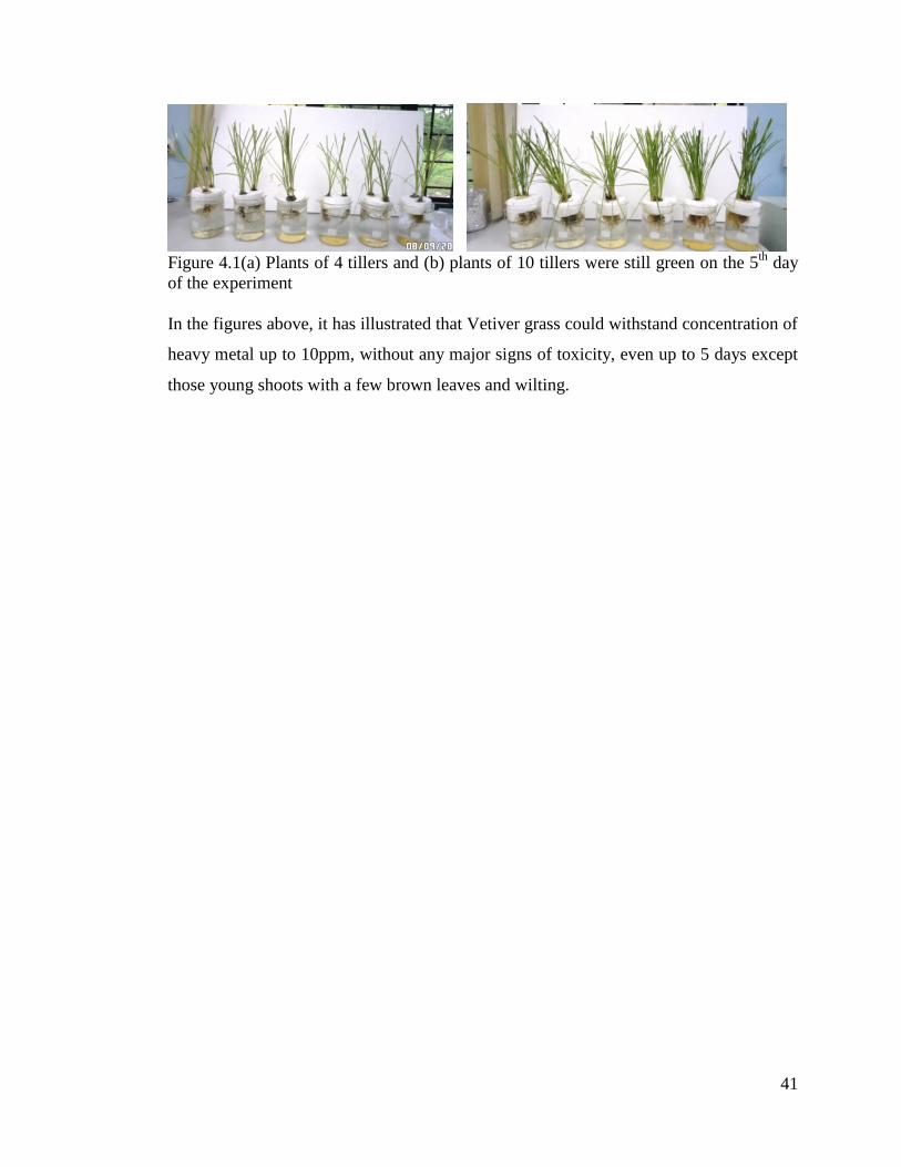
41

Figure 4.1(a) Plants of 4 tillers and (b) plants of 10 tillers were still green on the 5

th day

of the experiment

In the figures above, it has illustrated that Vetiver grass could withstand concentration of

heavy metal up to 10ppm, without any major signs of toxicity, even up to 5 days except

those young shoots with a few brown leaves and wilting.

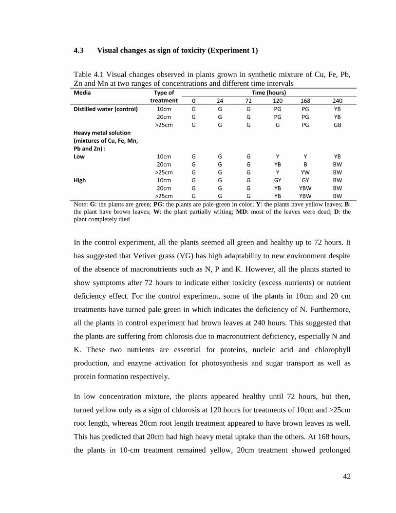
42

4.3 Visual changes as sign of toxicity (Experiment 1)

Table 4.1 Visual changes observed in plants grown in synthetic mixture of Cu, Fe, Pb,

Zn and Mn at two ranges of concentrations and different time intervals

Media Type of treatment

Time (hours)

0 24 72 120 168 240

Distilled water (control) 10cm 20cm

>25cm

G G G

G G G

G G G

PG PG G

PG PG PG

YB YB GB

Heavy metal solution (mixtures of Cu, Fe, Mn, Pb and Zn) : Low

10cm 20cm

>25cm

G G G

G G G

G G G

Y YB Y

Y B

YW

YB BW BW

High 10cm 20cm

>25cm

G G G

G G G

G G G

GY YB YB

GY YBW YBW

BW BW BW

Note: G: the plants are green; PG: the plants are pale-green in color; Y: the plants have yellow leaves; B:

the plant have brown leaves; W: the plant partially wilting; MD: most of the leaves were dead; D: the

plant completely died

In the control experiment, all the plants seemed all green and healthy up to 72 hours. It

has suggested that Vetiver grass (VG) has high adaptability to new environment despite

of the absence of macronutrients such as N, P and K. However, all the plants started to

show symptoms after 72 hours to indicate either toxicity (excess nutrients) or nutrient

deficiency effect. For the control experiment, some of the plants in 10cm and 20 cm

treatments have turned pale green in which indicates the deficiency of N. Furthermore,

all the plants in control experiment had brown leaves at 240 hours. This suggested that

the plants are suffering from chlorosis due to macronutrient deficiency, especially N and

K. These two nutrients are essential for proteins, nucleic acid and chlorophyll

production, and enzyme activation for photosynthesis and sugar transport as well as

protein formation respectively.

In low concentration mixture, the plants appeared healthy until 72 hours, but then,

turned yellow only as a sign of chlorosis at 120 hours for treatments of 10cm and >25cm

root length, whereas 20cm root length treatment appeared to have brown leaves as well.

This has predicted that 20cm had high heavy metal uptake than the others. At 168 hours,

the plants in 10-cm treatment remained yellow, 20cm treatment showed prolonged

43

deterioration by turning into brown leaves, and the plants in >25cm treatment has

already started to wilt. After 240 hours exposure, all the plants showed evidence of

further exposure by exhibiting signs of brown leaves, but the effects were greater at

20cm and >25cm treatments as the plants started to wilt.

In high concentration mixture, the plants all appeared to be healthy up to 72 hours.

However, at 120 hours till 240 hours onwards, the plants in 20cm and >25cm treatments

exhibited drastic changes as they showed chlorosis and already started to turn brown in

the expense of just 48 hours. They continued to exhibit signs of death by wilting. This

has suggested to be varying symptoms of heavy metal toxicity, especially Fe, Cu and Zn.

Although it can be seen that there is a difference in reducing tolerance as compared to

the low concentration, the plants were yet to show signs of necrosis (death) at the end of

the experiment. As for the 10cm treatment, it only started to show signs of prolonged

exposure of high concentration heavy metal at the end of the experiment.

In general, VG has shown its ability to adapt to high toxicity level of heavy metal in this

experiment that is asserted by the fact that it can tolerate high level of heavy metal

concentration (Truong, 2000; Truong, n.d.), whereby it did not even exhibit any signs of

death. The plants have only showed morphological symptoms such as chlorosis, brown

leaves due to prolonged heavy metal exposure and wilting. Other researchers have

indicated that different plant species would respond differently to metal toxicity. For

example, water lettuce appeared to be healthy up to Day 6with highest concentration of

5ppm (Kamaruzaman, 2011) and Phylidrum lanuginosum has showed toxicity

symptoms the next day when exposed to heavy metal treatment (Hanidza et al., 2011).

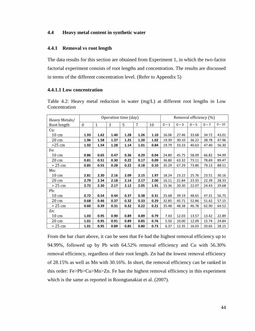
44

4.4 Heavy metal content in synthetic water

4.4.1 Removal vs root length

The data results for this section are obtained from Experiment 1, in which the two-factor

factorial experiment consists of root lengths and concentration. The results are discussed

in terms of the different concentration level. (Refer to Appendix 5)

4.4.1.1 Low concentration

Table 4.2: Heavy metal reduction in water (mg/L) at different root lengths in Low

Concentration

From the bar chart above, it can be seen that Fe had the highest removal efficiency up to

94.99%, followed up by Pb with 64.52% removal efficiency and Cu with 56.30%

removal efficiency, regardless of their root length. Zn had the lowest removal efficiency

of 28.15% as well as Mn with 30.16%. In short, the removal efficiency can be ranked in

this order: Fe>Pb>Cu>Mn>Zn. Fe has the highest removal efficiency in this experiment

which is the same as reported in Roongtanakiat et al. (2007).

Heavy Metals/ Root length

Operation time (day) Removal efficiency (%)

0 1 3 5 7 10 0 – 1 0 – 3 0 – 5 0 – 7 0 – 10

Cu: 10 cm 1.93 1.62 1.40 1.28 1.26 1.10 16.06 27.46 33.68 34.72 43.01

20 cm 1.96 1.58 1.37 1.25 1.20 1.02 19.39 30.10 36.22 38.78 47.96

>25 cm 1.92 1.54 1.28 1.14 1.01 0.84 19.79 33.33 40.63 47.40 56.30

Fe: 10 cm 0.86 0.65 0.47 0.36 0.29 0.04 24.80 45.75 58.09 66.82 94.99

20 cm 0.81 0.51 0.30 0.22 0.17 0.09 36.80 63.32 73.11 78.69 89.47

> 25 cm 0.85 0.55 0.28 0.22 0.18 0.10 35.29 67.29 73.86 79.13 88.51

Mn: 10 cm 2.81 2.30 2.16 2.09 2.15 1.97 18.24 23.22 25.76 23.51 30.16

20 cm 2.79 2.34 2.18 2.14 2.17 2.00 16.11 21.84 23.35 22.39 28.33

> 25 cm 2.72 2.30 2.17 2.12 2.05 1.91 15.36 20.30 22.07 24.43 29.68

Pb: 10 cm 0.72 0.54 0.44 0.37 0.38 0.31 25.68 39.19 48.65 47.31 56.75

20 cm 0.68 0.46 0.37 0.32 0.33 0.29 32.85 45.71 52.86 51.42 57.15

> 25 cm 0.60 0.39 0.31 0.32 0.22 0.21 35.48 48.38 46.78 62.90 64.52

Zn: 10 cm 1.03 0.95 0.90 0.89 0.89 0.79 7.43 12.03 13.57 13.42 22.89

20 cm 1.01 0.95 0.91 0.89 0.85 0.76 5.50 10.00 12.09 15.74 24.84

> 25 cm 1.01 0.95 0.89 0.85 0.80 0.73 6.37 12.35 16.03 20.65 28.15

45

Theoretically, it is assumed that the removal rate of heavy metal would increase as the

root length increases due to higher surface area for metal absorption by the root into the

plants. All of the plants in this experiment illustrated a trend whereby the removal

efficiency had increased when the root length increased, except for Fe and Mn. The Fe

removal efficiency has decreased as the root length increased; whereas Mn removal

efficiency was almost constant although the root length has increased.

Table 4.3 Compliance of data results in this experiment with MOH standard

Element Concentration, ppm Percent reduction, %

Compliance with the standard

MOH Standard

Initial Final (after 10 days)

Cu 1 1.94 0.99 48.97 yes Fe 1 0.84 0.08 90.48 yes Mn 0.2 2.77 1.96 29.24 no Pb 0.1 0.67 0.31 53.73 no Zn 5 1.02 0.76 25.49 yes

Based on the table above, it has shown that only Cu, Fe and Zn have met the

requirement for the MOH quality standard. In fact, it supposed that only Cu has

successfully been taken up by Vetiver as Fe and Zn have initial concentration of lower

than the MOH standard. As for Mn and Pb, both elements showed percent reduction,

however, it is suggested that they required a longer time to be taken up by the plant as

Mn is only micronutrient by plants, whereas Pb is not required for plant growth but a

toxicity at high concentration (McCauley, 2011; Bennett, 1993, as cited in Khalil, 2011).

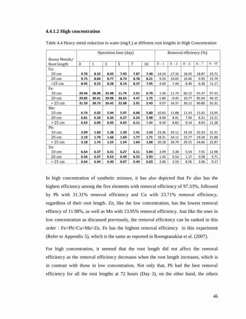
46

4.4.1.2 High concentration

Table 4.4 Heavy metal reduction in water (mg/L) at different root lengths in High Concentration

In high concentration of synthetic mixture, it has also depicted that Fe also has the

highest efficiency among the five elements with removal efficiency of 97.33%, followed

by Pb with 31.31% removal efficiency and Cu with 23.71% removal efficiency,

regardless of their root length. Zn, like the low concentration, has the lowest removal

effiency of 11.98%, as well as Mn with 13.95% removal efficiency. Just like the ones in

low concentration as discussed previously, the removal efficiency can be ranked in this

order : Fe>Pb>Cu>Mn>Zn. Fe has the highest removal efficiency in this experiment

(Refer to Appendix 5), which is the same as reported in Roongtanakiat et al. (2007).

For high concentration, it seemed that the root length did not affect the removal

efficiency as the removal efficiency decreases when the root length increases, which is

in contrast with those in low concentration. Not only that, Pb had the best removal

efficiency for all the root lengths at 72 hours (Day 3), on the other hand, the others

Heavy Metals/ Root length

Operation time (day) Removal efficiency (%)

0 1 3 5 7 10 0 – 1 0 – 3 0 – 5 0 – 7 0 – 10

Cu: 10 cm 9.70 8.32 8.02 7.92 7.87 7.40 14.23 17.32 18.35 18.87 23.71

20 cm 9.75 8.84 8.77 8.73 8.78 8.21 9.33 10.05 10.46 9.95 15.79

>25 cm 8.95 8.53 8.28 8.19 8.37 7.95 4.69 7.49 8.49 6.48 11.17

Fe: 10 cm 29.44 28.98 25.98 11.74 2.51 0.79 1.56 11.74 60.12 91.47 97.33

20 cm 29.85 30.41 29.98 26.63 4.47 1.75 -1.89 -0.45 10.77 85.04 94.15

> 25 cm 31.59 28.73 26.42 22.08 2.91 2.43 9.07 16.37 30.12 90.80 92.31

Mn: 10 cm 6.74 6.02 5.94 5.97 6.00 5.80 10.65 11.88 11.43 11.02 13.95

20 cm 6.81 6.20 6.20 6.27 6.24 5.98 8.98 8.91 7.94 8.31 12.21

> 25 cm 6.64 6.09 6.05 6.03 6.11 5.88 8.30 8.82 9.14 8.03 11.38

Pb: 10 cm 2.09 1.60 1.38 1.39 1.41 1.43 23.36 34.11 33.18 32.24 31.31

20 cm 2.19 1.79 1.66 1.69 1.77 1.71 18.31 24.11 22.77 19.20 21.88

> 25 cm 2.18 1.74 1.55 1.54 1.64 1.68 20.18 28.70 29.15 24.66 22.87

Zn: 10 cm 6.64 6.37 6.41 6.27 6.11 5.84 3.99 3.38 5.54 7.91 11.98

20 cm 6.56 6.47 6.53 6.49 6.53 5.93 1.42 0.54 1.17 0.58 9.71

> 25 cm 6.64 6.44 6.40 6.07 6.44 6.03 3.06 3.59 8.56 3.06 9.17

47

heavy metal element had the highest removal efficiency at 240 hours which is Day 10 –

the final day of the experiment.

Based on that Roongtanakiat (2007), the order was Fe>Mn>Zn>Cu>Pb in which Zn and

Mn have the higher plant uptake as compared to this experiment. This could be due to

the fact that excessive iron has reduced the zinc uptake and excessive zinc has reduced

the manganese uptake (Malvi, 2011).

Table 4.5 Compliance of data results in this experiment with MOH standard

Element Concentration, ppm Percent reduction, %

Compliance with the standard

MOH Standard

Initial Final (after 10 days)

Cu 1 9.47 7.85 17.11 no Fe 1 30.29 1.66 94.52 no Mn 0.2 6.73 5.89 12.48 no Pb 0.1 2.15 1.61 25.12 no Zn 5 6.61 5.93 10.29 no

Based on the table above, it has shown that all the elements did not meet the requirement

for the MOH quality standard. This is because the initial concentration of these elements

are very high, hence it is suggested that they required a longer time to be taken up by the

plant although there are high percent reduction, especially in Fe.

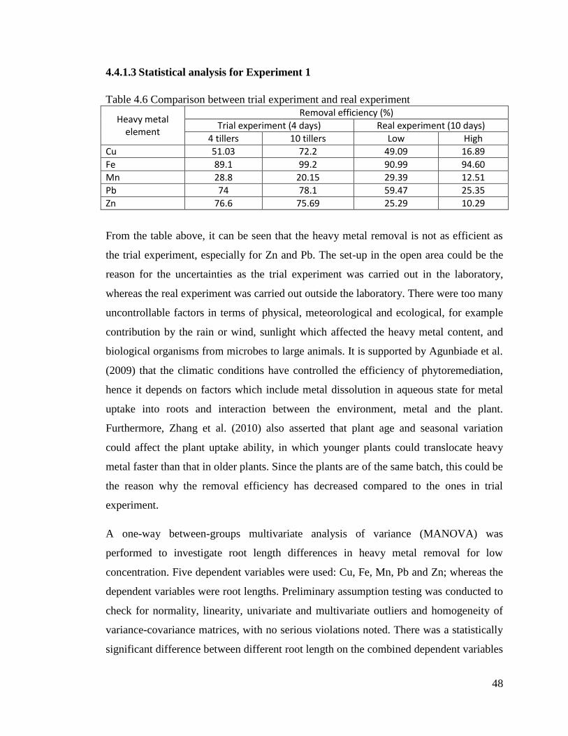
48

4.4.1.3 Statistical analysis for Experiment 1

Table 4.6 Comparison between trial experiment and real experiment

Heavy metal element

Removal efficiency (%)

Trial experiment (4 days) Real experiment (10 days)

4 tillers 10 tillers Low High

Cu 51.03 72.2 49.09 16.89

Fe 89.1 99.2 90.99 94.60

Mn 28.8 20.15 29.39 12.51

Pb 74 78.1 59.47 25.35

Zn 76.6 75.69 25.29 10.29

From the table above, it can be seen that the heavy metal removal is not as efficient as

the trial experiment, especially for Zn and Pb. The set-up in the open area could be the

reason for the uncertainties as the trial experiment was carried out in the laboratory,

whereas the real experiment was carried out outside the laboratory. There were too many

uncontrollable factors in terms of physical, meteorological and ecological, for example

contribution by the rain or wind, sunlight which affected the heavy metal content, and

biological organisms from microbes to large animals. It is supported by Agunbiade et al.

(2009) that the climatic conditions have controlled the efficiency of phytoremediation,

hence it depends on factors which include metal dissolution in aqueous state for metal

uptake into roots and interaction between the environment, metal and the plant.

Furthermore, Zhang et al. (2010) also asserted that plant age and seasonal variation

could affect the plant uptake ability, in which younger plants could translocate heavy

metal faster than that in older plants. Since the plants are of the same batch, this could be

the reason why the removal efficiency has decreased compared to the ones in trial

experiment.

A one-way between-groups multivariate analysis of variance (MANOVA) was

performed to investigate root length differences in heavy metal removal for low

concentration. Five dependent variables were used: Cu, Fe, Mn, Pb and Zn; whereas the

dependent variables were root lengths. Preliminary assumption testing was conducted to

check for normality, linearity, univariate and multivariate outliers and homogeneity of

variance-covariance matrices, with no serious violations noted. There was a statistically

significant difference between different root length on the combined dependent variables

49

which are the heavy metal elements, F (10, 22) = 5.532, p < 0.005; Wilks’ Lambda =

0.081; partial eta squared = 0.715. A separate ANOVA was conducted for each

dependent variable, with each ANOVA evaluated at an alpha level of 0.01, using

Bonferroni adjustment. Based on the Tests of Between-Subjects Effects table in

Appendix 6, there was no significant difference between different root length (10cm,

20cm and >25cm) in the removal of each heavy metal. This may be due to low interval

between the root length as well as harvesting period, hence, it could be the contribution

for results insignificance although it could be seen that there could be relationship

between root length and the removal efficiency. This is suggested because most of the

studies only harvest the plants after a certain period of time in weeks or months

(Ladislas, 2013; Roongtanakiat, 2007; Roongtanakiat, 2001). Pearson product-moment

correlation coefficient was done to investigate the relationship, however, there was no

correlation as p>0.05 (Appendix 7).

Another MANOVA was also performed for high concentration. There was no

statistically significant difference between different root length on the combined

dependent variables which are the heavy metal elements, F (10, 22) = 1.316, p = 0.282;

Wilks’ Lambda = 0.392; partial eta squared = 0.374. A separate ANOVA was conducted

for each dependent variable, with each ANOVA evaluated at an alpha level of 0.01,

using Bonferroni adjustment. Based on the Tests of Between-Subjects Effects table in

Appendix 8, there was no significant difference between different root length in the

removal of each heavy metal for High concentration.

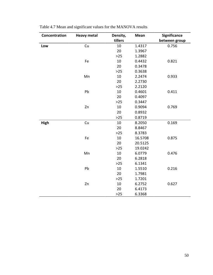
50

Table 4.7 Mean and significant values for the MANOVA results

Concentration Heavy metal Density, tillers

Mean Significance between group

Low Cu 10 1.4317 0.756 20 1.3967

>25 1.2882 Fe 10 0.4432 0.821

20 0.3478 >25 0.3638

Mn 10 2.2474 0.933 20 2.2730

>25 2.2120 Pb 10 0.4601 0.411

20 0.4097 >25 0.3447

Zn 10 0.9094 0.769

20 0.8932

>25 0.8719

High Cu 10 8.2050 0.169 20 8.8467

>25 8.3783 Fe 10 16.5708 0.875

20 20.5125 >25 19.0242

Mn 10 6.0779 0.476 20 6.2818

>25 6.1341 Pb 10 1.5510 0.216

20 1.7981 >25 1.7201

Zn 10 6.2752 0.627 20 6.4173

>25 6.3368

51

4.4.2 Removal vs density

The data results for this section are obtained from Experiment 2, in which the two-factor

factorial experiment consists of density (number of density) and concentration. The

results were discussed in terms of the different concentration level in sub-chapters below

(Refer to Appendix 10).

4.4.2.1 Low concentration

Table 4.8 Heavy metal reduction in water (mg/l) at different number of vetiver (density)

for low concentration

Based on Figure 4.7 above, it can be seen that Fe had the highest removal efficiency up

to 85.28%, followed up by Pb with 76.39% removal efficiency and Cu with 67.07%

removal efficiency, regardless of their density. Zn had the lowest removal efficiency of

38.06% as well as Mn with 40.52%. In short, the removal efficiency can be ranked in

this order: Fe>Pb>Cu>Mn>Zn. Fe has the highest removal efficiency in this experiment

which is the same as reported in Roongtanakiat et al. (2007).

Heavy

Metals/

No. of

vetiver

Operation time (day) Removal efficiency (%)

0 1 3 5 7 10 0 – 1 0 – 3 0 – 5 0 – 7 0 – 10

Cu:

25 1.96 1.75 1.66 1.57 1.51 1.31 10.71 15.31 19.90 22.96 33.16

50 1.94 1.51 1.30 1.20 1.13 0.98 22.16 32.99 38.14 41.75 49.33

100 1.98 1.24 0.65 0.82 0.80 0.65 37.37 66.97 58.79 59.60 67.07

Fe:

25 0.83 0.69 0.52 0.36 0.14 0.13 16.69 37.33 57.14 83.43 84.27

50 0.79 0.54 0.28 0.19 0.16 0.13 32.11 65.11 76.11 79.90 84.20

100 0.82 0.33 0.12 0.15 0.14 0.12 59.75 84.91 81.96 82.58 85.28

Mn:

25 2.90 2.41 2.37 2.33 2.28 2.07 16.88 18.13 19.50 21.12 28.50

50 2.82 2.31 2.21 2.14 2.15 1.99 18.28 21.63 24.08 23.75 29.30

100 2.90 2.48 2.06 2.09 2.03 1.72 14.25 28.93 28.01 29.90 40.52

Pb:

25 0.68 0.59 0.46 0.48 0.33 0.34 14.28 32.85 29.99 51.42 50.00

50 0.63 0.45 0.33 0.24 0.32 0.21 29.24 47.69 61.54 49.24 66.16

100 0.70 0.32 0.20 0.30 0.21 0.17 54.16 72.22 56.94 69.44 76.39

Zn:

25 1.05 1.01 0.99 0.97 0.96 0.84 3.50 5.50 7.90 9.03 20.35

50 1.02 0.95 0.92 0.90 0.88 0.78 6.52 9.37 12.14 13.17 23.24

100 1.04 0.94 0.81 0.82 0.79 0.65 10.22 22.61 21.23 24.08 38.06

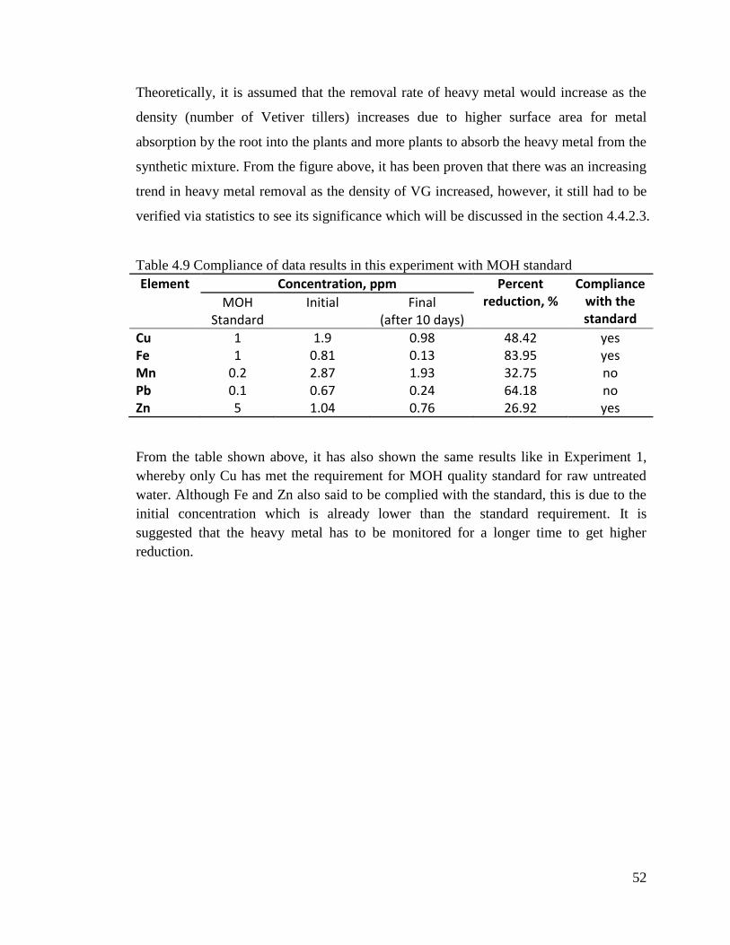
52

Theoretically, it is assumed that the removal rate of heavy metal would increase as the

density (number of Vetiver tillers) increases due to higher surface area for metal

absorption by the root into the plants and more plants to absorb the heavy metal from the

synthetic mixture. From the figure above, it has been proven that there was an increasing

trend in heavy metal removal as the density of VG increased, however, it still had to be

verified via statistics to see its significance which will be discussed in the section 4.4.2.3.

Table 4.9 Compliance of data results in this experiment with MOH standard

Element Concentration, ppm Percent reduction, %

Compliance with the standard

MOH Standard

Initial Final (after 10 days)

Cu 1 1.9 0.98 48.42 yes Fe 1 0.81 0.13 83.95 yes Mn 0.2 2.87 1.93 32.75 no Pb 0.1 0.67 0.24 64.18 no Zn 5 1.04 0.76 26.92 yes

From the table shown above, it has also shown the same results like in Experiment 1,

whereby only Cu has met the requirement for MOH quality standard for raw untreated

water. Although Fe and Zn also said to be complied with the standard, this is due to the

initial concentration which is already lower than the standard requirement. It is

suggested that the heavy metal has to be monitored for a longer time to get higher

reduction.

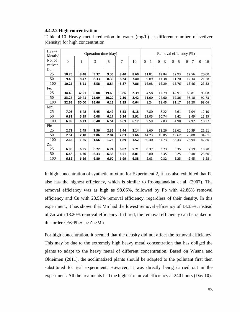
53

4.4.2.2 High concentration

Table 4.10 Heavy metal reduction in water (mg/L) at different number of vetiver

(density) for high concentration

In high concentration of synthetic mixture for Experiment 2, it has also exhibited that Fe

also has the highest efficiency, which is similar to Roongtanakiat et al. (2007). The

removal efficiency was as high as 98.06%, followed by Pb with 42.86% removal

efficiency and Cu with 23.52% removal efficiency, regardless of their density. In this

experiment, it has shown that Mn had the lowest removal efficiency of 13.35%, instead

of Zn with 18.20% removal efficiency. In bried, the removal efficiency can be ranked in

this order : Fe>Pb>Cu>Zn>Mn.

For high concentration, it seemed that the density did not affect the removal efficiency.

This may be due to the extremely high heavy metal concentration that has obliged the

plants to adapt to the heavy metal of different concentration. Based on Wuana and

Okieimen (2011), the acclimatized plants should be adapted to the pollutant first then

substituted for real experiment. However, it was directly being carried out in the

experiment. All the treatments had the highest removal efficiency at 240 hours (Day 10).

Heavy

Metals/

No. of

vetiver

Operation time (day) Removal efficiency (%)

0 1 3 5 7 10 0 – 1 0 – 3 0 – 5 0 – 7 0 – 10

Cu:

25 10.75 9.48 9.37 9.36 9.40 8.60 11.81 12.84 12.93 12.56 20.00

50 9.40 8.47 8.33 8.30 8.24 7.40 9.89 11.38 11.70 12.34 21.28

100 10.25 8.51 8.58 8.84 8.87 7.86 16.98 16.29 13.76 13.46 23.32

Fe:

25 34.49 32.91 30.08 19.69 3.86 2.39 4.58 12.79 42.91 88.81 93.08

50 33.27 29.41 25.09 10.20 2.30 2.42 11.60 24.60 69.36 93.10 92.73

100 32.69 30.00 26.66 6.16 2.55 0.64 8.24 18.45 81.17 92.20 98.06

Mn:

25 7.03 6.48 6.45 6.49 6.53 6.18 7.80 8.22 7.61 7.04 12.10

50 6.81 5.99 6.08 6.17 6.24 5.91 12.05 10.74 9.42 8.49 13.35

100 6.89 6.23 6.40 6.54 6.69 6.17 9.59 7.03 4.98 2.92 10.37

Pb:

25 2.72 2.49 2.36 2.35 2.44 2.14 8.60 13.26 13.62 10.39 21.51

50 2.54 2.18 2.06 2.04 2.03 1.66 14.23 18.85 19.62 20.00 34.61

100 2.66 1.85 1.66 1.78 1.89 1.52 30.40 37.73 33.33 28.94 42.86

Zn:

25 6.98 6.95 6.72 6.74 6.82 5.71 0.37 3.73 3.35 2.19 18.20

50 6.48 6.30 6.33 6.33 6.51 8.01 2.80 2.35 2.25 -0.48 -23.60

100 6.82 6.69 6.80 6.60 6.99 6.38 2.03 0.32 3.25 -2.45 6.58

54

Based on that Roongtanakiat (2007), the order was Fe>Mn>Zn>Cu>Pb in which Zn and

Mn have the higher plant uptake as compared to this experiment. This could be due to

the fact that excessive iron has reduced the zinc uptake and excessive zinc has reduced

the manganese uptake (Malvi, 2011).

Table 4.11. Compliance of data results in this experiment with MOH standard

Element Concentration, ppm Percent reduction, %

Compliance with the standard

MOH Standard

Initial Final (after 10 days)

Cu 1 10.13 7.95 21.52 no Fe 1 33.48 1.82 94.56 no Mn 0.2 6.91 6.09 11.87 no Pb 0.1 2.64 1.77 32.95 no Zn 5 6.76 6.7 0.89 no

Based on the table above, all the heavy metal element did not meet the standard

requirement for raw untreated water quality. Although there are high percent reduction,

especially for Fe, they failed to meet the standard as the initial concentration was very

high to simulate the real condition in the river. It is predicted that they could meet the

requirement if the experiment is monitored after a long time since most of the studies

carried out in long terms have significance for their results such as in Ladislas et al.

(2013) and Roongtanakiat (2007).

55

4.4.2.3 Statistical analysis for Experiment 2

Table 4.12 Comparison between trial experiment and real experiment

Heavy metal element

Removal efficiency (%)

Trial experiment (4 days) Real experiment (10 days)

4 tillers 10 tillers Low High

Cu 51.03 72.2 49.9 21.5

Fe 89.1 99.2 84.6 94.6

Mn 28.8 20.15 32.8 11.9

Pb 74 78.1 64.2 33.0

Zn 76.6 75.69 27.2 8.3

From the table above, it can be seen that the heavy metal removal is not as efficient as

the trial experiment, especially for Zn. The set-up in the open area could be the reason

for the uncertainties as the trial experiment was carried out in the laboratory, whereas the

real experiment was carried out outside the laboratory. According to Agunbiade et al.

(2009) that the climatic conditions have controlled the efficiency of phytoremediation,

hence it depends on factors which include metal dissolution in aqueous state for metal

uptake into roots and interaction between the environment, metal and the plant. In this

experiment, here were too many uncontrollable factors in terms of physical,

meteorological and ecological, for example contribution by the rain or wind, sunlight

which affected the heavy metal content, and biological organisms from microbes to large

animals. Furthermore, Zhang et al. (2010) also asserted that plant age and seasonal

variation could affect the plant uptake ability, in which younger plants could translocate

heavy metal faster than that in older plants. Since the plants are of the same batch, this

could be the reason why the removal efficiency has decreased compared to the ones in

trial experiment.

A one-way between-groups multivariate analysis of variance (MANOVA) was

performed to investigate density differences in heavy metal removal for Low

concentration. Five dependent variables were used: Cu, Fe, Mn, Pb and Zn; whereas the

dependent variables were density. Preliminary assumption testing was conducted to

check for normality, linearity, univariate and multivariate outliers, and homogeneity of

variance-covariance matrices, with no serious violations noted. There was a statistically

significant difference between different densities on the combined dependent variables

56

which are the heavy metal elements, F (10, 22) = 2.904, p = 0.018; Wilks’ Lambda =

0.186; partial eta squared = 0.569. A separate ANOVA was conducted for each

dependent variable, with each ANOVA evaluated at an alpha level of 0.01, using

Bonferroni adjustment. Based on the Tests of Between-Subjects Effects table in

Appendix 9, there was no significant difference between different densities (25 tillers,

50 tillers and 100 tillers) in the removal of each heavy metal although it can be observed

that there is an increasing trend of removal efficiency when the density increased.

MANOVA was also performed for High concentration. There was a statistically

significant difference between combined dependent variables which are the heavy metal

elements, F (10, 22) = 5.460, p < 0.005; Wilks’ Lambda = 0.082; partial eta squared =

0.713. A separate ANOVA was conducted for each dependent variable, with each

ANOVA evaluated at an alpha level of 0.01, using Bonferroni adjustment. Based on the

Tests of Between-Subjects Effects table in Appendix 10, there was no significant

difference between different densities in the removal of each heavy metal.

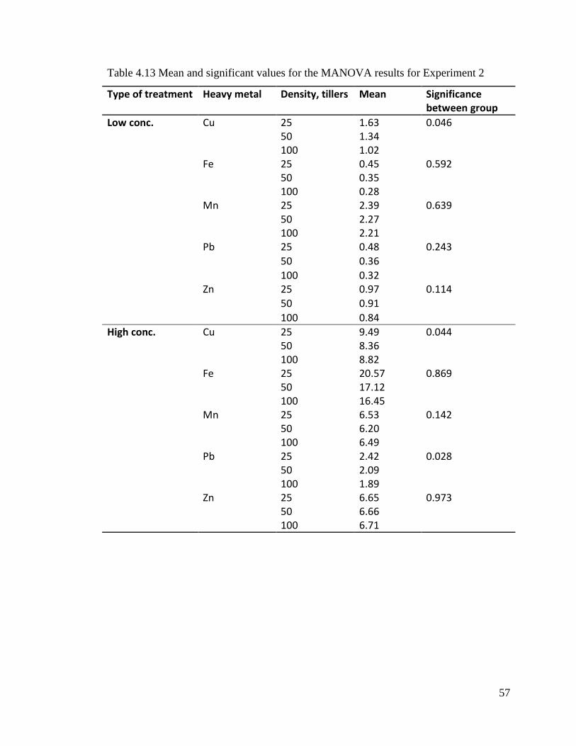
57

Table 4.13 Mean and significant values for the MANOVA results for Experiment 2

Type of treatment Heavy metal Density, tillers Mean Significance between group

Low conc. Cu 25 1.63 0.046 50 1.34 100 1.02

Fe 25 0.45 0.592 50 0.35 100 0.28

Mn 25 2.39 0.639 50 2.27 100 2.21

Pb 25 0.48 0.243

50 0.36

100 0.32 Zn 25 0.97 0.114

50 0.91

100 0.84

High conc. Cu 25 9.49 0.044 50 8.36 100 8.82

Fe 25 20.57 0.869 50 17.12 100 16.45

Mn 25 6.53 0.142 50 6.20 100 6.49

Pb 25 2.42 0.028 50 2.09 100 1.89

Zn 25 6.65 0.973 50 6.66 100 6.71

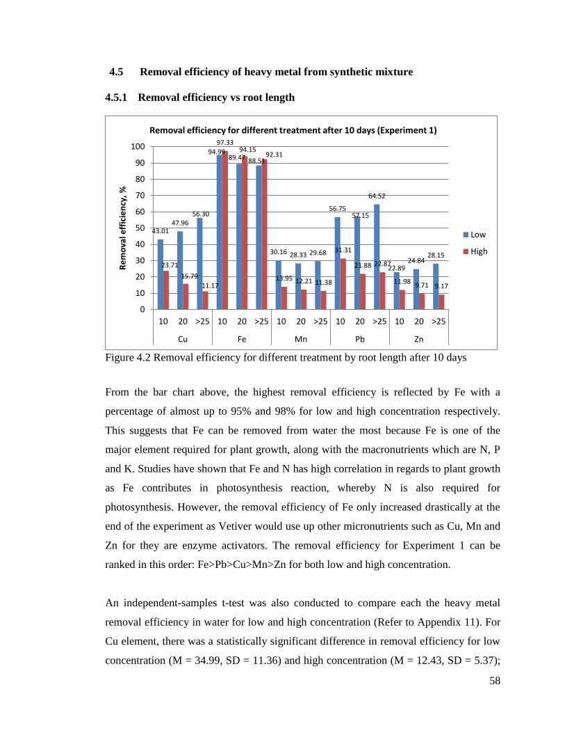
58

4.5 Removal efficiency of heavy metal from synthetic mixture

4.5.1 Removal efficiency vs root length

Figure 4.2 Removal efficiency for different treatment by root length after 10 days

From the bar chart above, the highest removal efficiency is reflected by Fe with a

percentage of almost up to 95% and 98% for low and high concentration respectively.

This suggests that Fe can be removed from water the most because Fe is one of the

major element required for plant growth, along with the macronutrients which are N, P

and K. Studies have shown that Fe and N has high correlation in regards to plant growth

as Fe contributes in photosynthesis reaction, whereby N is also required for

photosynthesis. However, the removal efficiency of Fe only increased drastically at the

end of the experiment as Vetiver would use up other micronutrients such as Cu, Mn and

Zn for they are enzyme activators. The removal efficiency for Experiment 1 can be

ranked in this order: Fe>Pb>Cu>Mn>Zn for both low and high concentration.

An independent-samples t-test was also conducted to compare each the heavy metal

removal efficiency in water for low and high concentration (Refer to Appendix 11). For

Cu element, there was a statistically significant difference in removal efficiency for low

concentration (M = 34.99, SD = 11.36) and high concentration (M = 12.43, SD = 5.37);

43.01 47.96

56.30

94.99 89.47 88.51

30.16 28.33 29.68

56.75 57.15

64.52

22.89 24.84

28.15

23.71

15.79

11.17

97.33 94.15

92.31

13.95 12.21 11.38

31.31

21.88 22.87

11.98 9.71 9.17

0

10

20

30

40

50

60

70

80

90

100

10 20 >25 10 20 >25 10 20 >25 10 20 >25 10 20 >25

Cu Fe Mn Pb Zn

Re

mo

val e

ffic

ien

cy,

%

Removal efficiency for different treatment after 10 days (Experiment 1)

Low

High

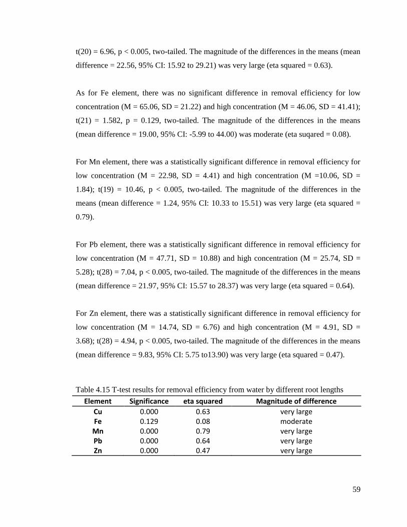
59

t(20) = 6.96, p < 0.005, two-tailed. The magnitude of the differences in the means (mean

difference = 22.56, 95% CI: 15.92 to 29.21) was very large (eta squared = 0.63).

As for Fe element, there was no significant difference in removal efficiency for low

concentration (M = 65.06, SD = 21.22) and high concentration (M = 46.06, SD = 41.41);

t(21) = 1.582, p = 0.129, two-tailed. The magnitude of the differences in the means

(mean difference = 19.00, 95% CI: -5.99 to 44.00) was moderate (eta suqared = 0.08).

For Mn element, there was a statistically significant difference in removal efficiency for

low concentration (M = 22.98, SD = 4.41) and high concentration (M =10.06, SD =

1.84); t(19) = 10.46, p < 0.005, two-tailed. The magnitude of the differences in the

means (mean difference = 1.24, 95% CI: 10.33 to 15.51) was very large (eta squared =

0.79).

For Pb element, there was a statistically significant difference in removal efficiency for

low concentration (M = 47.71, SD = 10.88) and high concentration (M = 25.74, SD =

5.28); t(28) = 7.04, p < 0.005, two-tailed. The magnitude of the differences in the means

(mean difference = 21.97, 95% CI: 15.57 to 28.37) was very large (eta squared = 0.64).

For Zn element, there was a statistically significant difference in removal efficiency for

low concentration (M = 14.74, SD = 6.76) and high concentration (M = 4.91, SD =

3.68); t(28) = 4.94, p < 0.005, two-tailed. The magnitude of the differences in the means

(mean difference = 9.83, 95% CI: 5.75 to13.90) was very large (eta squared = 0.47).

Table 4.15 T-test results for removal efficiency from water by different root lengths

Element Significance eta squared Magnitude of difference

Cu 0.000 0.63 very large Fe 0.129 0.08 moderate Mn 0.000 0.79 very large Pb 0.000 0.64 very large Zn 0.000 0.47 very large

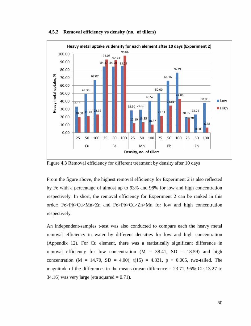
60

4.5.2 Removal efficiency vs density (no. of tillers)

Figure 4.3 Removal efficiency for different treatment by density after 10 days

From the figure above, the highest removal efficiency for Experiment 2 is also reflected

by Fe with a percentage of almost up to 93% and 98% for low and high concentration

respectively. In short, the removal efficiency for Experiment 2 can be ranked in this

order: Fe>Pb>Cu>Mn>Zn and Fe>Pb>Cu>Zn>Mn for low and high concentration

respectively.

An independent-samples t-test was also conducted to compare each the heavy metal

removal efficiency in water by different densities for low and high concentration

(Appendix 12). For Cu element, there was a statistically significant difference in

removal efficiency for low concentration (M = 38.41, SD = 18.59) and high

concentration (M = 14.70, SD = 4.00); t(15) = 4.831, p < 0.005, two-tailed. The

magnitude of the differences in the means (mean difference = 23.71, 95% CI: 13.27 to

34.16) was very large (eta squared = 0.71).

33.16

49.33

67.07

84.27 84.20 85.28

28.50 29.30

40.52

50.00

66.16

76.39

20.35 23.24

38.06

20.00 21.28 23.32

93.08 92.73

98.06

12.10 13.35 10.37

21.51

34.61

42.86

18.20

0.00

6.58

0.00

10.00

20.00

30.00

40.00

50.00

60.00

70.00

80.00

90.00

100.00

25 50 100 25 50 100 25 50 100 25 50 100 25 50 100

Cu Fe Mn Pb Zn

He

avy

me

tal u

pta

ke, %

Density, no. of tillers

Heavy metal uptake vs density for each element after 10 days (Experiment 2)

Low

High

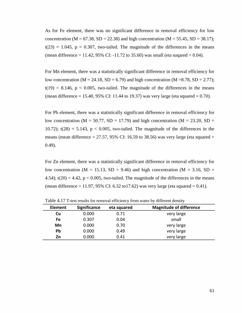
61

As for Fe element, there was no significant difference in removal efficiency for low

concentration (M = 67.38, SD = 22.38) and high concentration (M = 55.45, SD = 38.17);

t(23) = 1.045, p = 0.307, two-tailed. The magnitude of the differences in the means

(mean difference = 11.42, 95% CI: -11.72 to 35.60) was small (eta suqared = 0.04).

For Mn element, there was a statistically significant difference in removal efficiency for

low concentration (M = 24.18, SD = 6.79) and high concentration (M =8.78, SD = 2.77);

t(19) = 8.146, p < 0.005, two-tailed. The magnitude of the differences in the means

(mean difference = 15.40, 95% CI: 11.44 to 19.37) was very large (eta squared = 0.70).

For Pb element, there was a statistically significant difference in removal efficiency for

low concentration (M = 50.77, SD = 17.79) and high concentration (M = 23.20, SD =

10.72); t(28) = 5.143, p < 0.005, two-tailed. The magnitude of the differences in the

means (mean difference = 27.57, 95% CI: 16.59 to 38.56) was very large (eta squared =

0.49).

For Zn element, there was a statistically significant difference in removal efficiency for

low concentration (M = 15.13, SD = 9.46) and high concentration (M = 3.16, SD =

4.54); t(20) = 4.42, p < 0.005, two-tailed. The magnitude of the differences in the means

(mean difference = 11.97, 95% CI: 6.32 to17.62) was very large (eta squared = 0.41).

Table 4.17 T-test results for removal efficiency from water by different density

Element Significance eta squared Magnitude of difference

Cu 0.000 0.71 very large Fe 0.307 0.04 small Mn 0.000 0.70 very large Pb 0.000 0.49 very large Zn 0.000 0.41 very large

62

4.6 Heavy metal uptake by plant parts (only for Experiment 1)

4.6.1 Heavy metal content in plant root

Figure 4.4 Heavy metal content in root for Low concentration in terms of dry weight

basis. Error bars represent SDs; n=6.

In low concentration, Fe had the highest concentration of 7260 mg/kg in the root for all

treatments at Day 7. Pb content in the root was the second highest with 2829 mg/kg,

followed closely by Cu at 2620 mg/kg. Mn and Zn had the lowest content in the root

among the 5 elements with 2420 mg/kg and 1586 mg/kg respectively. Overall, all

elements had the highest content in the root at 168 hours (Day 7), except for Mn and Zn

were highest at the early stage of the experiment. This suggested that plant absorbed

most of the nutrients such as Mn and Zn first, as both Mn and Zn are responsible for

enzyme activation for photosynthesis and growth respectively (McCauley, 2011;

Bennett (1993), as cited in Khalil, 2011). In short, the heavy metal content in the root for

low concentration can be ranked in this order: Fe>Pb>Cu>Mn>Zn, which has

corresponded with the removal efficiency from the synthetic mixture.

0

1000

2000

3000

4000

5000

6000

7000

8000

L10 L20 L30 L10 L20 L30 L10 L20 L30 L10 L20 L30 L10 L20 L30

Cu Fe Mn Pb Zn

Co

nce

ntr

atio

n, m

g/kg

Heavy metal content in root for Low concentration

Day 0

Day 1

Day 3

Day 5

Day 7

Day 10

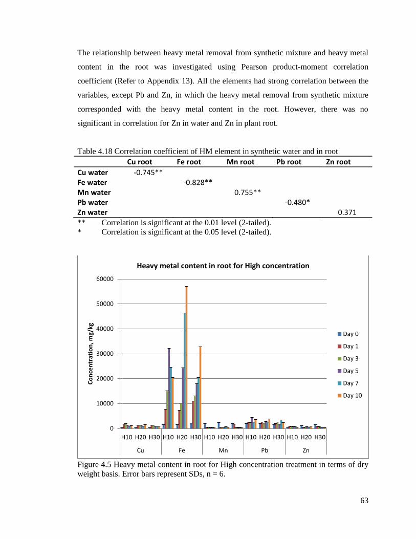
63

The relationship between heavy metal removal from synthetic mixture and heavy metal

content in the root was investigated using Pearson product-moment correlation

coefficient (Refer to Appendix 13). All the elements had strong correlation between the

variables, except Pb and Zn, in which the heavy metal removal from synthetic mixture

corresponded with the heavy metal content in the root. However, there was no

significant in correlation for Zn in water and Zn in plant root.

Table 4.18 Correlation coefficient of HM element in synthetic water and in root

Cu root Fe root Mn root Pb root Zn root

Cu water -0.745** Fe water -0.828** Mn water 0.755** Pb water -0.480* Zn water 0.371

** Correlation is significant at the 0.01 level (2-tailed).

* Correlation is significant at the 0.05 level (2-tailed).

Figure 4.5 Heavy metal content in root for High concentration treatment in terms of dry

weight basis. Error bars represent SDs, n = 6.

0

10000

20000

30000

40000

50000

60000

H10 H20 H30 H10 H20 H30 H10 H20 H30 H10 H20 H30 H10 H20 H30

Cu Fe Mn Pb Zn

Co

nce

ntr

atio

n, m

g/kg

Heavy metal content in root for High concentration

Day 0

Day 1

Day 3

Day 5

Day 7

Day 10

64

In high concentration, Fe had the highest concentration of 57000 mg/kg in the root for

at 240 hours (Day 10). Pb content in the root was the second highest with 4487 mg/kg,

followed by Mn at 2420 mg/kg and Cu at 1900 mg/kg. Zn had the lowest content in the

root among the 5 elements with 1586 mg/kg. All elements had different concentration in

the root for high concentration treatment. However, Fe still exhibited constant behavior,

in which its content is normally high at the end of the experiment as the plant would use

up other micronutrients first than Fe. This is because Fe is used for photosynthesis

reactions but the plant required essential micronutrients for enzyme activation before

photosynthesis can be taken place. In brief, the heavy metal content in the root for high

concentration can be ranked in this order: Fe>Pb>Mn >Cu >Zn, which is different than

that of removal efficiency from the synthetic mixture.

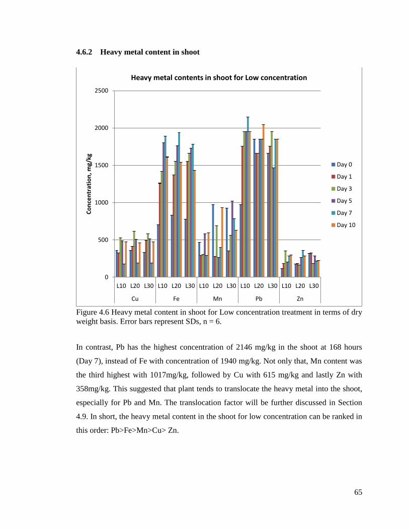
65

4.6.2 Heavy metal content in shoot

Figure 4.6 Heavy metal content in shoot for Low concentration treatment in terms of dry

weight basis. Error bars represent SDs, n = 6.

In contrast, Pb has the highest concentration of 2146 mg/kg in the shoot at 168 hours

(Day 7), instead of Fe with concentration of 1940 mg/kg. Not only that, Mn content was

the third highest with 1017mg/kg, followed by Cu with 615 mg/kg and lastly Zn with

358mg/kg. This suggested that plant tends to translocate the heavy metal into the shoot,

especially for Pb and Mn. The translocation factor will be further discussed in Section

4.9. In short, the heavy metal content in the shoot for low concentration can be ranked in

this order: Pb>Fe>Mn>Cu> Zn.

0

500

1000

1500

2000

2500

L10 L20 L30 L10 L20 L30 L10 L20 L30 L10 L20 L30 L10 L20 L30

Cu Fe Mn Pb Zn

Co

nce

ntr

atio

n, m

g/kg

Heavy metal contents in shoot for Low concentration

Day 0

Day 1

Day 3

Day 5

Day 7

Day 10

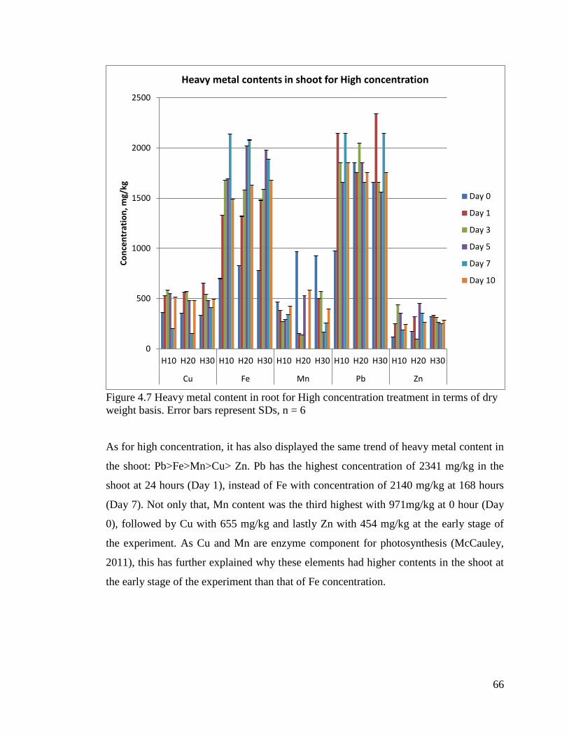
66

Figure 4.7 Heavy metal content in root for High concentration treatment in terms of dry

weight basis. Error bars represent SDs, n = 6

As for high concentration, it has also displayed the same trend of heavy metal content in

the shoot: Pb>Fe>Mn>Cu> Zn. Pb has the highest concentration of 2341 mg/kg in the

shoot at 24 hours (Day 1), instead of Fe with concentration of 2140 mg/kg at 168 hours

(Day 7). Not only that, Mn content was the third highest with 971mg/kg at 0 hour (Day

0), followed by Cu with 655 mg/kg and lastly Zn with 454 mg/kg at the early stage of

the experiment. As Cu and Mn are enzyme component for photosynthesis (McCauley,

2011), this has further explained why these elements had higher contents in the shoot at

the early stage of the experiment than that of Fe concentration.

0

500

1000

1500

2000

2500

H10 H20 H30 H10 H20 H30 H10 H20 H30 H10 H20 H30 H10 H20 H30

Cu Fe Mn Pb Zn

Co

nce

ntr

atio

n, m

g/kg

Heavy metal contents in shoot for High concentration

Day 0

Day 1

Day 3

Day 5

Day 7

Day 10

67

Table 4.19 Highest concentration recorded in past literature and my experiment for

hydroponic condition and requirement to be classified as hyperaccumulator

Heavy metal

element

Concentration, mg/kg DW (Highest)

Hydroponic condition* Real experiment Hyperaccumulator**

root shoot root shoot shoot

Cu 900 700 2620 655 ≥ 1000

Fe - - 57000 2140 -

Mn - - 2420 1017 10000

Pb ≥ 10000 ≥ 3350 4487 2341 ≥1000

Zn >10000 >10000 1586 454 10000 * Source from Anjum et al., 2012

** Unique characteristic to be classified as hyperaccumulator

According to Agunbiade (2009), the special characteristic of hyperaccumulators is that

the shoot would accumulate at least 1000 mg/kg dry mass for As, Pb, Cu, Ni and Co.

The Pb content in this experiment for both low and high concentration is more than 1000

mg/kg DW (Ladislas et al., 2013; Agunbiade et al, 2009), thus it can be concluded that

Vetiver can be known as Pb hyperaccumulator, which corresponds to the statement in

Danh et al. (2009).

4.6.3 Heavy metal accumulation in plant

Table 4.20 Heavy metal accumulation in plant (mg/kg after 10) days

Metals/ Treatment Condition

Metal accumulation in Root

Metal accumulation in Leaves Whole plant accumulation

10cm 20cm >25cm 10cm 20cm >25cm 10cm 20cm >25cm

Cu: Low conc. 1445 1663 1703 112 106 142 1557 1769 1845

High conc. 835 1233 576 155 121 161 990 1354 737

Fe: Low conc. 2450 3780 3390 910 710 650 3360 4490 4040

High conc. 18890 55390 30680 790 800 900 19680 56190 31580

Mn: Low conc. NA NA NA 128 NA NA NA NA NA

High conc. NA NA NA NA NA NA NA NA NA

Pb: Low conc. 293 NA 781 976 195 195 1269 NA 976

High conc. 1658 1756 781 878 NA 98 2536 1659 879

Zn: Low conc. 224 NA NA 186 110 NA 410 NA NA

High conc. 76 NA NA 129 86 NA 205 NA NA

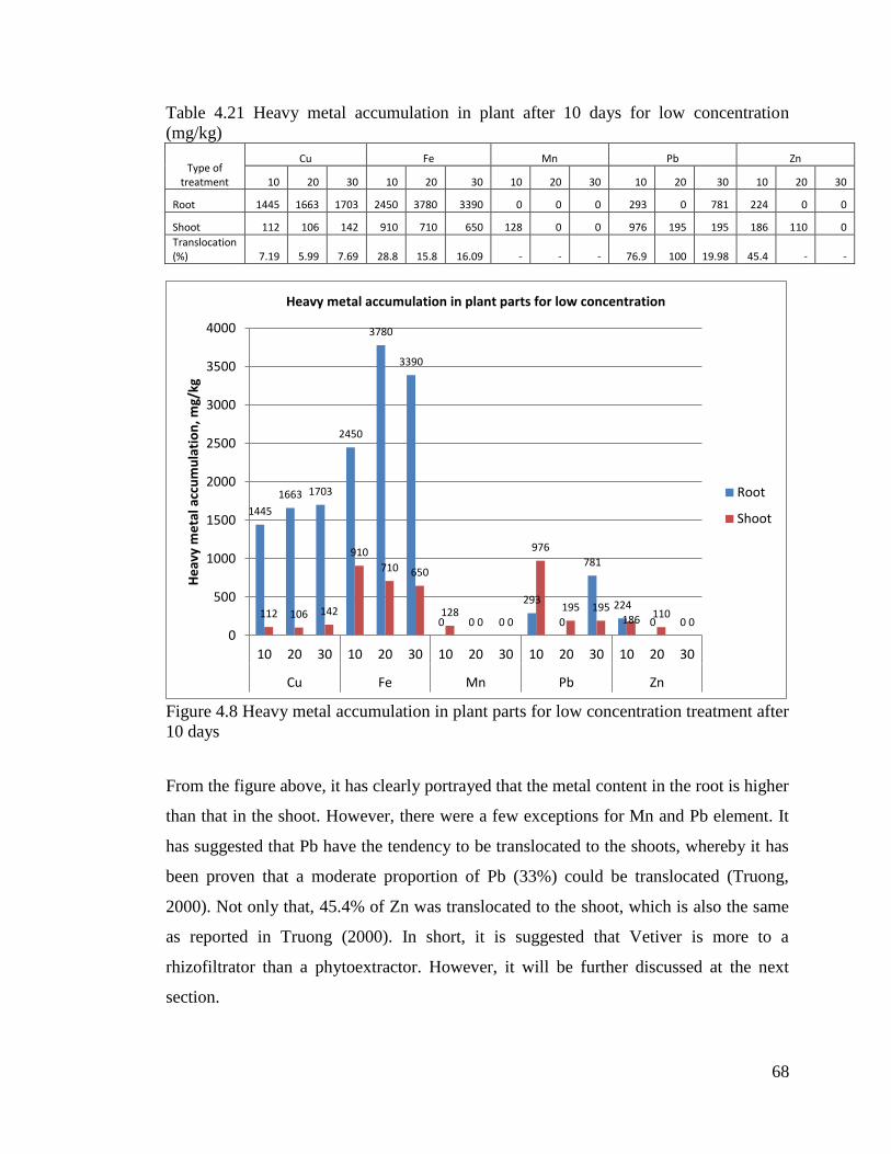
68

Table 4.21 Heavy metal accumulation in plant after 10 days for low concentration

(mg/kg)

Type of treatment

Cu Fe Mn Pb Zn

10 20 30 10 20 30 10 20 30 10 20 30 10 20 30

Root 1445 1663 1703 2450 3780 3390 0 0 0 293 0 781 224 0 0

Shoot 112 106 142 910 710 650 128 0 0 976 195 195 186 110 0

Translocation (%) 7.19 5.99 7.69 28.8 15.8 16.09 - - - 76.9 100 19.98 45.4 - -

Figure 4.8 Heavy metal accumulation in plant parts for low concentration treatment after

10 days

From the figure above, it has clearly portrayed that the metal content in the root is higher

than that in the shoot. However, there were a few exceptions for Mn and Pb element. It

has suggested that Pb have the tendency to be translocated to the shoots, whereby it has

been proven that a moderate proportion of Pb (33%) could be translocated (Truong,

2000). Not only that, 45.4% of Zn was translocated to the shoot, which is also the same

as reported in Truong (2000). In short, it is suggested that Vetiver is more to a

rhizofiltrator than a phytoextractor. However, it will be further discussed at the next

section.

1445

1663 1703

2450

3780

3390

0 0 0

293

0

781

224

0 0 112 106 142

910

710 650

128 0 0

976

195 195 186

110 0

0

500

1000

1500

2000

2500

3000

3500

4000

10 20 30 10 20 30 10 20 30 10 20 30 10 20 30

Cu Fe Mn Pb Zn

He

avy

me

tal a

ccu

mu

lati

on

, mg/

kg

Heavy metal accumulation in plant parts for low concentration

Root

Shoot

69

Furthermore, it can be seen that Mn and Zn have less or no accumulation in the shoot or

root. This is because there was a significant Mn and Zn content in the control plants,

which contained an average value of 2147.3 ± 236 mg/kg dw and 787.67 ± 278 mg/kg

dw; and 995.33 ± 620 mg/kg dw and 204 ± 105 mg/kg dw in root and shoot respectively.

An independent-samples t-test was also conducted to compare each the heavy metal

accumulation in plants by different part for low concentration (Refer to Appendix 15).

All the elements have shown statistically significant difference in heavy metal content at

different plant parts.

Table 4.22 T-tests results for heavy metal accumulation in different plant part after 10

days for Low concentration treatment

Element Significance eta squared Magnitude of difference

Cu p < 0.0005 0.64 very large Fe p < 0.0005 0.58 very large Mn 0.001 0.30 very large Pb p < 0.0005 0.36 very large Zn p < 0.0005 0.47 very large

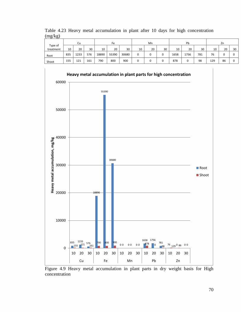
70

Table 4.23 Heavy metal accumulation in plant after 10 days for high concentration

(mg/kg)

Type of treatment

Cu Fe Mn Pb Zn

10 20 30 10 20 30 10 20 30 10 20 30 10 20 30

Root 835 1233 576 18890 55390 30680 0 0 0 1658 1756 781 76 0 0

Shoot 155 121 161 790 800 900 0 0 0 878 0 98 129 86 0

Figure 4.9 Heavy metal accumulation in plant parts in dry weight basis for High

concentration

835 1233 576

18890

55390

30680

0 0 0

1658 1756 781

76 0 0 155 121 161 790 800 900

0 0 0 878 0 98 129 86 0

0

10000

20000

30000

40000

50000

60000

10 20 30 10 20 30 10 20 30 10 20 30 10 20 30

Cu Fe Mn Pb Zn

He

avy

me

tal a

ccu

mu

lati

on

, mg/

kg

Heavy metal accumulation in plant parts for high concentration

Root

Shoot

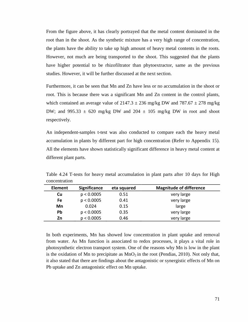
71

From the figure above, it has clearly portrayed that the metal content dominated in the

root than in the shoot. As the synthetic mixture has a very high range of concentration,

the plants have the ability to take up high amount of heavy metal contents in the roots.

However, not much are being transported to the shoot. This suggested that the plants

have higher potential to be rhizofiltrator than phytoextractor, same as the previous

studies. However, it will be further discussed at the next section.

Furthermore, it can be seen that Mn and Zn have less or no accumulation in the shoot or

root. This is because there was a significant Mn and Zn content in the control plants,

which contained an average value of 2147.3 ± 236 mg/kg DW and 787.67 ± 278 mg/kg

DW; and 995.33 ± 620 mg/kg DW and 204 ± 105 mg/kg DW in root and shoot

respectively.

An independent-samples t-test was also conducted to compare each the heavy metal

accumulation in plants by different part for high concentration (Refer to Appendix 15).

All the elements have shown statistically significant difference in heavy metal content at

different plant parts.

Table 4.24 T-tests for heavy metal accumulation in plant parts after 10 days for High

concentration

Element Significance eta squared Magnitude of difference

Cu p < 0.0005 0.51 very large Fe p < 0.0005 0.41 very large Mn 0.024 0.15 large Pb p < 0.0005 0.35 very large Zn p < 0.0005 0.46 very large

In both experiments, Mn has showed low concentration in plant uptake and removal

from water. As Mn function is associated to redox processes, it plays a vital role in

photosynthetic electron transport system. One of the reasons why Mn is low in the plant

is the oxidation of Mn to precipitate as MnO2 in the root (Pendias, 2010). Not only that,

it also stated that there are findings about the antagonistic or synergistic effects of Mn on

Pb uptake and Zn antagonistic effect on Mn uptake.

72

4.6.4 Statistical analysis for heavy metal concentration in plants

An independent-samples t-test was also conducted to compare each the heavy metal

accumulation in plant roots for different concentration. All the elements have shown

statistically significant difference in heavy metal content in plant root, except for Mn

and Zn (Refer to Appendix 16).

Table 4.25 T-tests for heavy metal accumulation in plant root for different concentration

Element Significance eta squared Magnitude of difference

Cu 0.008 0.21 large Fe 0.001 0.34 very large Mn 0.135 0.06 moderate Pb 0.030 0.14 large Zn 0.471 0.02 small

Another independent-samples t-test was also conducted to compare each the heavy metal

accumulation in plant shoots for different concentration. The results have exhibited that

all the elements had no significant difference in heavy metal content in plant shoot

(Refer to Appendix 17).

Table 4.26 T-tests for heavy metal accumulation in plant shoots for different

concentration

Element Significance eta squared Magnitude of difference

Cu 0.365 0.02 small Fe 0.597 0.01 small Mn 0.063 0.10 moderate Pb 0.774 0.002 very small Zn 0.262 0.04 small

From these two analysis, it can be concluded that plant would take up heavy metal from

synthetic mixture, which has different heavy metal level, at different amount and rate

into the plant roots. However, the ability to translocate them into the shoot is not

affected by the heavy metal level in the synthetic mixture.

73

4.7 Bioconcentration factor (BCF) [only for Experiment 1]

Figure 4.10 Bioconcentration factor (BCF) for Low concentration treatment

Figure 4.11 Bioconcentration factor (BCF) for High concentration treatment

430 454 566

37,442

18,118

14,592

303 467 330

6,249 6,999 8,635

380 379 308 0

5000

10000

15000

20000

25000

30000

35000

40000

L10 L20 L30 L10 L20 L30 L10 L20 L30 L10 L20 L30 L10 L20 L30

Cu Fe Mn Pb Zn

Bio

nco

nce

ntr

atio

n f

acto

r Bioconcentration factor for low concentration

Day 0

Day 1

Day 3

Day 5

Day 7

Day 10

853

466 651

0

1,517

939

1,309

54 70 58 62

1,898

934

691

73 98 68

1,292

1,029 1,047

42 47

0

200

400

600

800

1000

1200

1400

1600

1800

2000

H10 H20 H30 H10 H20 H30 H10 H20 H30 H10 H20 H30 H10 H20 H30

Cu Fe Mn Pb Zn

Bio

con

cen

trat

ion

fac

tor

Bioconcentration factor for high concentration

Day 0

Day 1

Day 3

Day 5

Day 7

Day 10

74

According to Agunbiade et al. (2009), the enrichment factor > 1, which is represented by

concentration in plant/habitat), is one of the feature of an accumulator. Enrichment

factor is also known as bioconcentration factor (BCF). Based on Zhang et al. (2014),

BCF>1 indicates the accumulation of heavy metals in the shoot. In the two figures

above, it has clearly displayed that all the BCFs are more than 1 as the scale could go up

to hundreds. Therefore, it can be concluded that Vetiver has the ability to translocate

heavy metal in the shoot.

4.8 Translocation factor (TF) [only for Experiment 1]

Figure 4.12 Translocation factor (TF) for Low concentration treatment

0

0.2

0.4

0.6

0.8

1

1.2

1.4

1.6

L10 L20 L30 L10 L20 L30 L10 L20 L30 L10 L20 L30 L10 L20 L30

Cu Fe Mn Pb Zn

Tran

slo

cati

on

fac

tor

Translocation factor for Low Concentration

Day 0

Day 1

Day 3

Day 5

Day 7

Day 10

TF=1

75

Figure 4.13 Translocation factor (TF) for High concentration treatment

According to Agunbiade et al. (2009) and Zhang et al., 2014), translocation factor (TF)

>1 is also one of the features for an accumulator. Based on the two figures above, most

of the TF are below 1. This indicates that Vetiver prefers to accumulate heavy metal in

the root more than in the shoot, although the bioconcentration factor in the previous

section has shown that Vetiver has the ability to translocate the heavy metal into the

shoot. In contrast, there a few exceptions, whereby Mn and Pb have TF > 1 in both low

and high concentration treatment. This means that Pb can accumulate Pb in the shoot as

VG has high affinity towards lead (Danh et al., 2009), however, it is in contrast with Lai

& Chen (2004) saying that vetiver cannot take up Pb in soil even at high concentration

level of 1000 mg/kg in the soil. This suggests that vetiver would behave differently in

terms of heavy metal uptake in different environmental condition.

The important findings of this experiment is that since not much heavy metal are

translocated into the shoot, its shoots can be used as food for grazing animals or mulch,

as reported in Anjum (2013) and Truong (2000).

0

0.2

0.4

0.6

0.8

1

1.2

1.4

1.6

1.8

H10 H20 H30 H10 H20 H30 H10 H20 H30 H10 H20 H30 H10 H20 H30

Cu Fe Mn Pb Zn

Tran

slo

cati

on

fac

tor

Translocation factor for High concentration

Day 0

Day 1

Day 3

Day 5

Day 7

Day 10

TF = 1

76

CHAPTER 5

SUMMARY OF FINDINGS, CONCLUSIONS, PROJECT LIMITATIONS AND

RECOMMENDATIONS FOR FUTURE RESEARCH

5.1 Summary of findings

This project is carried out in order to explore and understand more in-depth about the

use of phytoremediation technique in water by using Vetiver grass (VG). The objectives

are (1) to assess the efficiency of phytoremediation technique by using VG in water, (2)

to determine the rate of pollutant uptake by VG in varying pollutant concentrations, root

length and density of VG, and (3) to evaluate the removal efficiency of heavy metal

uptake by VG. This project is believed to have successfully met the objectives stated in

this project.

5.2 Conclusions

For plant cultivation; it is better to grow them at these conditions:(1) avoid strong UV

rays/ preferably sheltered with sufficient amount of sunlight, (2) acidic condition below

5 to prevent growth or invasion of fungus and other organisms, (3) provide aeration to

enhance the growth, (4) avoid using fertilizer that causes the pH to be alkaline, (5) high

electrical conductivity ranging from 2mS/cm to 8 mS/cm, and (6) trimming to enhance

new growth.

During the experiment, the toxicity symptoms of the Vetiver grass (VG) towards the

treatment for Experiment 1 have been observed. VG is said to have high adaptability to

polluted environment as all the plants still looked green and healthy up to 3 days.

However, the symptoms started to show up, either due to malnutrition (Controls) or

over-nourishment (LCT and HCT), such as chlorosis, browning of leaves due to

prolonged exposure and then wilting as a sign of necrosis. In a nutshell, none of the

plants died during the experiment even if wilting was present as it only occurred in a

very small amount.

77

The order of heavy metal removal efficiency from water for both high and low

concentration in Experiment 1 are: LCT [Fe(90.48) >Pb(53.73) >Cu(48.97) >Mn(29.24)

>Zn(25.49)]; HCT [Fe(94.52) >Pb(25.12) >Cu(17.11) >Mn(12.48) >Zn(10.29)]. As for

Experiment 2, the order was also the same as in Experiment 1: LCT [Fe(83.95)

>Pb(64.18) >Cu(48.42) >Mn(32.75) >Zn(26.92)] and HCT [Fe(98.06) >Pb(42.86)

>Cu(23.52) >Mn(13.35) >Zn(18.20)]. This order has corresponded to the heavy metal

accumulation in the root for Low Concentration Treatment (LCT), but not for High

Concentration Treatment (HCT) of Experiment 1 due to the inconsistent uptake of Cu

and Mn by the plants. The order of heavy metal accumulation by roots in mg/kg DW

basis are as follows: LCT [Fe(7260) >Pb(2829) >Cu(2620) >Mn(2420) >Zn(1586)];

HCT [Fe(57000) >Pb(4487) >Mn(2420) >Cu(1900) >Zn(1586)]. The order of heavy

metal accumulation by shoots in DW basis for both low and high concentration are as

follows: LCT [Pb(2146) >Fe(1940) >Mn(1017) >Cu(615) > Zn(358)]; HCT [Pb(2341)

>Fe(2140) >Mn(971) >Cu(655) > Zn(454)]. It is suspected to be the antagonistic or

synergistic effect of between Fe and Zn, Mn and Pb and Mn and Zn, which has affected

the uptake. Not only that, the difference in habitat (soil or water) would affect the

bioavailability of the heavy metal.

Throughout these experiments, it has been found that there were no significance in

removal efficiency by different root length and Vetiver density. This might be due to the

low interval between the root lengths, hence there are obvious significance when the

experiment is done for only 10 days. As compared to the trial experiment, the removal

efficiency is ranked in this order: Fe>Pb>Zn>Cu>Mn, which is different from the real

experiment, the possible reasons could be due to the climatic condition, seasonal

variation and the plant age. It is an unexpected findings that the heavy metal in the HCT

did not meet the quality standard set by MOH for the potable water. It is the same goes

to LCT, except for Cu. Although there were high removal efficiencies in some heavy

element, the residual concentration has not met the MOH water quality standard as the

experiment is carried out for only 10 days.

From this experiment, Vetiver grass is best to known as rhizofiltrator instead of phyto-

extractor due to its ability to accumulate heavy metal in the roots than in the shoot

78

although all the data results have shown BCF>1 but TF<1 as well. In contrast, there is a

finding, whereby Vetiver is a Pb hyper-accumulator as most of the heavy metal

concentrated in the shoot. Although VG is not a hyper-accumulator except for Pb, VG is

still a good accumulator for phytoremediation. Not only that, this experiment also shows

that Vetiver grass behave differently in heavy metal uptake, depending on the type of

environment (soil or water) and physical condition (pH, salinity, electrical conductivity,

etc.).

5.3 Project Limitations

The report would present information that is as accurate and valid as possible. However,

there are several potential limitations that would affect the accuracy and precision of

some information in the report includes:

The time allocated to complete the entire research project to be carried

out was 8 months (March to October) but the plants only arrived in the

middle of June. Hence, the project is delayed and only left 5 months to do

the project.

As the project has been delayed, the interval for harvesting was also

shortened. This could be the reason why there were no significance in

doing this experiment.

The plants were supposed to arrive with the root lengths requested (15cm,

45cm and 60cm) earlier on during the plant ordering but they all arrived

with root lengths of 12cm so they have to be cultivated once again to get

the specified root lengths for the experiment.

In order to get the root length specified for the experiment, a lot of time

has been wasted in growing the plants. Almost 5 months is spent in plant

cultivation, however the longest root obtained was only up to 35cm.

Hence, the experimental design has to be altered slightly. It was

79

suggested that it could also be the reason why there were no significance

in the experimental results as their root length interval was too small.

The plants are cultivated in water as part of plant acclimatization and due

to absence of suitable land for cultivation, thus the plant growth would be

slower as compared to planting in the soil.

The synthetic mixture prepared was done by using dilution of minerals

salts. Due to this method, the synthetic mixture obtained did not reach the

specified concentration. This may be due to calculation error or the large

volume of synthetic mixture which has contributed to more errors.

However, the concentration for each element could be obtained for trial

experiment.

Since the budget provided was limited, the experimental set-up at the

open area, which is difficult to control as the surroundings are

biodiversity-rich environment, could be reason of some data

uncertainties as it could be affected by rain water or other contributors

such as the air pollutants and other organisms.

The researcher’s main area of study in the discipline of Environmental

Science and Technology is not adequate to analyse certain aspects of the

research subject such as the plant cultivation, the study of the plant

growth and the handling of the plants as well as experimental preparation

and analysis of the samples.

80

5.4 Recommendations for Future Research

In order to improve the limitations faced in this project, in which the data results did not

turn out as expected, there are several recommendations to be suggested in regards of

future research. It might be a good opportunity in order to help explore more on the

pollutant uptake mechanism in terms of toxicity, tolerance towards heavy metals and

accumulation of heavy metals in the plants. The recommendations are listed as shown

below:

The projects should be carried out in a longer time length as the time required for

plant cultivation as well as plant acclimatization would take a very long time,

especially the plant cultivation which would take up to at least 6 months.

The plant cultivation should be done in soil as VG grow faster in the soil than

water; whereas the plant acclimatization in water can be done for a week time up

to a month before the experiment. If there is no land to plant, the soil attached to

plants should not be washed out during plant cultivation in water.

It is suggested to use higher interval of root length (15cm or even up to 30cm)

for the experiment, maybe it would produce a more significant results as the

interval for this experiment is only up to 10cm, which has not much different.

It is suggested to increase the harvesting time interval as plants need time to

grow and adapt to the synthetic mixture condition. Harvesting at a longer interval

of time may produce better results than that in this project.

For synthetic mixture preparation, it is better to use standard solution to obtain

the specified concentration as the concentration using metal salts dilution might

be difficult to control, especially the ones found in this experiment although the

trial experiment shows a good results. It is suggested that the larger volume has

incurred more errors in preparing the solution.

It is better to use metals salts in the form of nitrates as other salt forms like

sulphates, chlorides and others might cause the physical or chemical reaction

between the specified heavy metal element in the experiment with the salts.

81

Not only that, the method used for acid digestion has to be validated as it is

modified from Hanidza et al. (2011) although the results obtained from the

experiment has acceptable RSD values as well as constant expected results.

The time length of the experiment should be longer to see the effective of

treatment by the Vetiver grass in order to remove heavy metal from the water to

meet the MOH quality standard for raw untreated water.

82

REFERENCES

Agunbiade, F.O., Olu-Owolabi, B.I., Adebowale, K.O. (2009). Phytoremediation

potential of Eichornia crassipes in metal-contaminated coastal water. Bioresource

Technology, 100, 4521–4526. doi:10.1016/j.biortech.2009.04.011

Al-Badaii, F., Othman, M.S. & Gasim, M.B. (2013). Water Quality Assessment of the

Semenyih River, Selangor, Malaysia. Hindawi Publishing Corporation, Journal of

Chemistry, Article ID 871056. Retrieved from

http://dx.doi.org/10.1155/2013/871056

Ali, M.F., Heng, L.Y., Ratnam, W., Nais, J. &, Ripin, R. (2004). Metal Distribution and

Contamination of the Mamut River, Malaysia, Caused by Copper Mine

Discharge. Bull. Environ. Contam. Toxicol., 7, 535–542. DOI: 10.1007/s00128-

004-0462-5

Aliu, S., Jusufi, S., Daci, M. & Dehari, S. (2011). Seas, Ecological Balance and

Sustainable Environment. Heavy Metals in the Water of Lake Ohrid and in Fish

Species Belbica – Alburnus alburnus alborella de Filippi. H. Gökçekus¸ et al.

(eds.), Survival and Sustainability, Environmental Earth Sciences, 29. DOI

10.1007/978-3-540-95991.

Anjum, N.A., Pereira, M., Duarte, I.A.A., Umar, S. & Khan, N.A. (2013).

Phytotechnologies: Remediation of Environmental Contaminants (Eds.). Boca

Raton, Florida: Taylor & Francis.

Appelo, C.A.J., Postma, D. (1993). Geochemistry, Groundwater and Pollution. A. A.

Balkema Publishers, Rotterdam. p. 536.

Ashraf, M.A. & Maah, M.J. & Yusoff, I. (2013). Evaluation of Natural

Phytoremediation Process Occurring at Ex-tin Mining Catchment. Chiang Mai J.

Sci.; 40(2), 198-213. Retrieved from http://it.science.cmu.ac.th/ejournal/

Ashraf, M.A. & Maah, M.J. & Yusoff, I. (2011). Heavy metals accumulation in plants

growing in ex tin mining catchment. Int. J. Environ. Sci. Tech., 8 (2), 401-416.

Atta, M., Yaacob, W.Z.W., Jaafar, O. (2015). The potential impact of leachate-

contaminated groundwater of an ex-landfill site at Taman Beringin Kuala Lumpur,

Malaysia. Environ Earth Sci, 73, 3913–3923. DOI 10.1007/s12665-014-3675-x

ATSDR. (2011). Toxic Substances Portal. Retrieved from http://www.atsdr.cdc.gov

Bakar, A.F.A., Yusoff, I., Ng, T.F., Othman, F. & Ashraf, M.A. (2015). Cumulative

impacts of dissolved ionic metals on the chemical characteristics of river water

affected by alkaline mine drainage from the Kuala Lipis gold mine, Pahang,

Malaysia, Chemistry and Ecology, 31(1), 22-33, DOI:

10.1080/02757540.2014.950569

83

Bakar, A.F.A., Yusoff, I., Ng, T.F., Othman, F. & Ashraf, M.A. (2013). Arsenic, Zinc,

and Aluminium Removal from Gold Mine Wastewater Effluents and

Accumulation by Submerged Aquatic Plants (Cabomba piauhyensis, Egeria

densa, and Hydrilla verticillata). BioMed Research International. Article ID

890803

Bernama. (March 20, 2015). Thousands affected by water cut in Klang Valley. Free

Malaysia Today. Retrieved from http://www.freemalaysiatoday.com

Berghof. (n.d.). Theory of Sample Preparation Using Acid Digestion, Pressure Digestion

and Microwave Digestion (Microwave Decomposition). Berghof Products +

Instruments GmbH. Retrieved from http://www.berghof.com

Bian, B., Zhou, L.J., Li, L.,Lv, L. & Fan, Y.M. (2015). Risk assessment of heavy metals

in air, water, vegetables, grains, and related soils irrigated with biogas slurry in

Taihu Basin, China. Environ Sci Pollut Res, 22, 7794–7807. DOI

10.1007/s11356-015-4292-2

Biswas, A. K. & Tortajada, C. (2011) Water Quality Management: An Introductory

Framework. Int. J. Water Resources Development, 27(1), 5-11, doi:

10.1080/07900627.2010.547979

Bouraie, M.M.E., Barbary, A.A.E., Yehia, M.M. & Motawea, E.A. (2010). Heavy metal

concentrations in surface river water and bed sediments at Nile Delta in Egypt.

Suo 61(1): 1–12 — Research notes.

Carlos A. Harguinteguy, C.A., Cofr´e, M. N., Fern´andez-Cirelli, A., Pignata, M. L.

(2015). The macrophytes Potamogeton pusillus L. and Myriophyllum aquaticum

(Vell.) Verdc. as potential bioindicators of a river contaminated by heavy metals.

Microchemical Journal. doi: 10.1016/j.microc.2015.08.014

Chan, N. W. (2012). Managing urban rivers and water quality in Malaysia for

sustainable water resources. Wat. Res. Dev., 28(2), 343-354. doi:

10.1080/07900627.2012.668643

Chomchalow, N. (2003, January). The Role of Vetiver in Controlling Water Quantity

and Treating Water Quality: An Overview with Special Reference to Thailand.

Paper presented at the Fourth Thai National Conference on Vetiver, Bangkok. AU

J.T. 6(3): 145 – 161.

Cleophas, F. N., Isidore, F., Lee, K.H. & Bidin, K. (2013). Water quality status of

Liwagu River, Tambunan, Sabah, Malaysia. Journal Of Tropical Biology And

Conservation, 10: 67-73

Cunningham, S. D., Berti, W.R. & Huang, J.W. (1995). Remediation of Contaminated

Soils and Sludges by Green Plants. Battelle Press, Columbus, OH, 33 – 54.

84

Danh, L.T., Truong, P., Mammucari, R., Tran, T., & Foster, N. (2009). Vetiver Grass,

Vetiveria Zizanioides: A Choice Plant For Phytoremediation of Heavy Metals and

Organic Wastes. Int. J. of Phytoremediation, 11, 664-691. doi:

10.1080/15226510902787302

Darajeh, N., Idris, A., Truong, P., Aziz, A. A., Bakar, R. A., & Man, H. C. (2014).

Phytoremediation Potential of Vetiver System Technology for improving the

Quality of Palm Oil Mill Effluent. Advances in Materials Science and

Engineering. Vol. 4, Article ID 683579, http://dx.doi.org/10.1155/2014/683579

Department of Environment (DOE). (2003). Water quality management in Malaysia.

Kuala Lumpur: DOE Documents.

Dudai, N., Putievsky, E., Chaimovitch, D. & Ben-Hur, M. (2006). Growth management

of vetiver (Vetiveria zizanioides) under Mediterranean conditions. Journal of

Environmental Management, 81, 63 – 71.

Fingerman, M. & Nagabushanam, R. (2005). Bioremediation of Aquatic and Terrestrial

Ecosystem. USA: Science Publishers. University New Orleans, Louisiana.

Fulazzaky, M.A., Seong, T.W., & Masrin, M.I.M. (2010). Assessment of Water Quality

Status for the Selangor River in Malaysia. Water Air Soil Pollut., 205, 63–77. doi

10.1007/s11270-009-0056-2

Galal, T.M. & Shehata, H.S. (2014). Evaluation of the invasive macrophyte

Myriophyllum spicatum L. as a bioaccumulator for heavy metals in some

watercourses of Egypt. Ecological Indicators, 41, 209–214. Retrieved from

http://dx.doi.org/10.1016/j.ecolind.2014.02.004

Gupta, P., Roy, S., Mahindrakar, A.B. (2012). Treatment of Water Using Water

Hyacinth, Water Lettuce and Vetiver Grass - A Review. Resources and

Environment, 2(5), 202-215. doi: 10.5923/j.re.20120205.04

Hadibarata, T., Abdullah, F., Yusoff, A. R. M., Ismail, R., Azman, S. & Adnan, N.

(2012). Correlation Study between Land Use, Water Quality, and Heavy Metals

(Cd, Pb, and Zn) Content in Water and Green Lipped Mussels Perna viridis

(Linnaeus.) at the Johor Strait. Water Air Soil Pollut, 223. 3125–3136. DOI

10.1007/s11270-012-1095-7

Hanidza, T., Aris, A. Z., Somasundram, S. (2011). Potential Removal of Pb, Cu And Zn

by Phylidrum Lanuginosum in Aquatic Environment. Fresenius Environmental

Bulletin, Volume 20, 5a, 1262 – 1269.

Hatar, H., Rahim, S. A., Razi, W. M. & Sahrani, F. K. (2013). Heavy metals content in

acid mine drainage at abandoned and active mining area. AIP Conference

Proceedings, 1571, 641. doi: 10.1063/1.4858727

85

Havlin, J.L. & Soltanpour, P.N. (1980). A nitric acid plant tissue digest method for use

with inductively coupled plasma spectrometry. Communications in Soil Science

and Plant Analysis, 11, 10, 969 – 980. DOI:10.1080/00103628009367096

Hosier, S. & Bradley, L. (May, 1999). Guide to Symptoms of Plant Nutrient

Deficiencies. The University of Arizona Cooperative Extension. Publication

AZ1106 5/99

Hseu, Z.Y. (2004). Evaluating heavy metal contents in nine composts using four

digestion methods. Bioresource Technology, 95, 53–59.

doi:10.1016/j.biortech.2004.02.008

Huang, L., Bell, R.W., Dell, B. & Woodward, J. (2004). Rapid Nitric Acid Digestion of

Plant Material with an Open-vessel Microwave System. Communications In Soil

Science And Plant Analysis, 35, Nos. 3 & 4, pp. 427–440. DOI: 10.1081/CSS-

120029723

Ibrahim, N., Aziz, H.A., & Yusoff, M.S. (2015). Heavy metals concentration in river

and pumping well water for river bank filtration (rbf) system: case study in

Sungai Kerian. Jurnal Teknologi. 74(11), 59–67.

Idriss, A. A & Ahmad, A K. (2012). Concentration of selected heavy metals in water of

the Juru River, Penang, Malaysia. African Journal of Biotechnology, 11(33),

8234-8240. DOI: 10.5897/AJB11.3840

Ippolito, J.A. & Barbarick, K.A. (2000). Modified nitric acid plant tissue digest method.

Communications in Soil Science and Plant Analysis, 31, 15-16, 2473 – 2482.

DOI:10.1080/00103620009370602

Jopony, M. & Tongkul F. (2009). Acid Mine Drainages at Mamut Copper Mine, Sabah,

Malaysia. Borneo Science, 24, March 2009.

Kamaruzaman, N. (2011). Phytoremediation of Heavy Metals (Fe and Ni) in Water by

Pistia Stratiotes. (Unpublished degree dissertation). Universiti Putra Malaysia,

Malaysia.

Khalil, N.A.N.A. (2011). Phytoremediation of Heavy Metals and The Physical Changes

of Acacia Mangium Planted in Contaminated Soil From Indah Water Konsortium

(IWK). (Unpublished degree dissertation). Universiti Putra Malaysia, Malaysia.

Kidney, S. (1997). Phytoremediation may take root in Brownfields The Brownfields

Report. 2(14), 1 – 6

Kohušová, K., Havel, L., Vlasák, P. & Tonika, J. (2011). A long-term survey of heavy

metals and specific organic compounds in biofilms, sediments, and surface water

in a heavily affected river in the Czech Republic. Environ Monit Assess, 174,

555–572. DOI 10.1007/s10661-010-1478-4

86

Kusin, F.M., Muhammad, S. N. & Zahar, M.S.M. (2014). Limestone-Based Closed

Reactor For Passive Treatment of Highly Acidic Raw Water. International

Journal of Research In Earth & Environmental Sciences. 2,1, 13 – 23.

Kusin, F.M. (2013). A Review of the Importance of Hydraulic Residence Time on

Improved Design of Mine Water Treatment Systems. World Applied Sciences

Journal, 26 (10), 1316-1322. doi: 10.5829/idosi.wasj.2013.26.10.412

Ladislas, S., Gérente, C., Chazarenc, F., Brisson, J. & Andrès, Y. (2015). Floating

treatment wetlands for heavy metal removal in highway stormwater ponds.

Ecological Engineering, 80, 85–91. doi.org/10.1016/j.ecoleng.2014.09.115

Ladislas, S., Gérente, C., Chazarenc., F., Brisson, J., & Andrès, Y. (2013). Performances

of Two Macrophytes Species in Floating Treatment Wetlands for Cadmium,

Nickel, and Zinc Removal from Urban Stormwater Runoff. Water Air Soil

Pollution, 224:1408. DOI 10.1007/s11270-012-1408-x

Lai, H.Y. & Chen, Z.S. (2004). Effects of EDTA on solubility of cadmium, zinc, and

lead and their uptake by rainbow pink and vetiver grass. Chemosphere, 55, 421 –

430. Doi:10.1016/j.chemosphere.2003.11.009

Laing, G.D., Tack, F.M.G. & Verloo, M.G. (2003). Performance of selected destruction

methods for the determination of heavy metals in reed plants (Phragmites

australis). Analytica Chimica Acta , 497, 191–198. doi:10.1016/j.aca.2003.08.044

Lee, P. Monday April 22, 2013 MYT 6:16:23 PM. 49,000 still affected by water supply

disruption. http://www.thestar.com.my/News/Nation/2013/01/17

Lee, Y.H. & Stuebing, R.B. (1990). Heavy Metal Contamination in the River Toad, Bufo

juxtasper (Inger), Near a Copper Mine in East Malaysia. Bull. Environ. Contam.

Toxicol., 45, 272-279.

Li, G., Liu, G., Zhou, C., Chou, C.L., Zheng, L. &Wang, J. (2012). Spatial distribution

and multiple sources of heavy metals in the water of Chaohu Lake, Anhui, China.

Environ Monit Assess,184, 2763–2773. DOI 10.1007/s10661-011-2149-9

Ling, T.Y., Kho, C.P. & Lee, N. (2012). Spatial and Temporal Variations of Heavy

Metals in a Tropical River. World Applied Sciences Journal, 16 (4), 550-559.

Lu, X., Kruatrachue, M., Pokethitiyook, P. & Homyok, K. (2004). Removal of Cadmium

and Zinc by Water Hyacinth, Eichhornia crassipes. ScienceAsia, 30, 93-103.

DOI: 10.2306/scienceasia1513-1874.2004.30.093

Malvi, U. (2011). Interaction of micronutrients with major nutrients with special

reference to potassium. Karnataka J. Agric. Sci., 24, 1, 106-109. Retrieved from

http://www.inflibnet.ac.i

87

Mather-Gaspar, G & Anton, A. (2005). Phytoremediation study: Factors influencing

Heavy Metal Uptake of Plants. Proceedings of the 8th

Hungarian Congress on

Plant Physiology and the 6th

Hungarian Conference on Photosunthesis, 2005, 69 –

70.

McCauley, A. (June, 2011). Plant Nutrient Functions and Deficiency and Toxicity

Symptoms. Nutrient Management Module No. 9. 4449-9. Retrieved from

http://landresources.montana.edu/nm/documents/NM9.pdf

Moore, F., Esmaelli, K. & Keshavarzi, B. (2011). Assessment of Heavy Metals

Contamination in Stream Water and Sediments Affected by the Sungun Porphyry

Copper Deposit, East Azerbaijan Province, Northwest Iran. Water Qual Expo

Health, 3, 37–49. DOI 10.1007/s12403-011-0042-y

Muhammad, S.N., Kusin, F.M., Zahar, M.S.M., Madzlen, N.S. & Gaung, E.R. (2015).

Passive Treatment of Metal and Sulphate-Rich Acid Mine Drainage (AMD)

Using Mixed Limestone, Spent Mushroom Compost and Activated Sludge.

IJSRSET 151438, 1(4), 234 – 239

National Risk Management Research Laboratory (NRMRL) (2000). Introduction to

Phytoremediation. Environment Protection Agency. EPA/600/R-99/107.

Othman, F., Eldin, M. E. A., & Mohamed, I. (2012). Trend analysis of a tropical urban

river water quality in Malaysia. J. Environ. Monit., 14, 3164-3173. doi:

10.1039/c2em30676j

Orji, K.U., Sapari, N., Yusof, K.W., Asadpour, R. & Olisa, e. (2013). Comparative study

of water quality of rivers used for raw water supply & ex-mining lakes in Perak,

Malaysia. 4th International Conference on Energy and Environment 2013 (ICEE

2013). IOP Conf. Series: Earth and Environmental Science, 16.

doi:10.1088/1755-1315/16/1/012072

Payus, C., David, O. & Moh, P.Y. (2014). Bone Meal As Alternative Treatment For

Acidic And Metal Contaminated Acid Mine Drainage Water Effluent: Lab Scale.

American Journal of Environmental Science, 10,1, 61-73.

doi:10.3844/ajessp.2014.61.73

Pendias, A.K. (2010). Trace Elements in Soils and Plants (4th

ed.). Boca Raton, Florida:

Taylor & Francis.

Philips, D.P., Human, L.R.D. & Adams, J.B. (2015). Wetland plants as indicators of

heavy metal contamination. Marine Pollution Bulletin, 92, 227–232. Retrieved

from http://dx.doi.org/10.1016/j.marpolbul.2014.12.038

Pilon-Smits, E. (2005). Phytoremediation. Annu. Rev. Plant. Biol., 56, 15-39.

88

Prajapati, S.K., Meravi, N. & Singh, S. (2012). Phytoremediation of Chromium and

Cobalt using Pistia stratiotes: A sustainable approach. Proceedings of the

International Academy of Ecology and Environmental Sciences, 2(2), 136-138.

Prasanna, M. V., Praveena, S. M., Chidambaram, S., Nagarajan, R. & Elayaraja, A.

(2012). Evaluation of water quality pollution indices for heavy metal

contamination monitoring: a case study from Curtin Lake, Miri City, East

Malaysia. Environ Earth Sci, 67, 1987–2001. DOI 10.1007/s12665-012-1639-6

Punamiya, P., Datta, R., Sarkar, D., Barber, S., Patel, M. & Das, P (2010). Symbiotic

role of Glomus mosseae in phytoextraction of lead in vetiver grass [Chrysopogon

zizanioides (L.)] Journal of Hazardous Materials, 177, 465–474.

doi:10.1016/j.jhazmat.2009.12.056

Puyang, X., Gao, C., Han, L. (2015). Risk Assessment of Heavy Metals in Water and

Two Fish Species from Golf Course Ponds in Beijing, China. Bull Environ

Contam Toxicol, 94, 437–443. DOI 10.1007/s00128-015-1476-x

Rezania, S., Ponraj, M., Talaiekhozani, A., Mohamad, S.E., Din, M.F.M., Taib, S.M.,

Sabbagh, F. & Sairan, F.M. (2015). Perspectives of phytoremediation using water

hyacinth for removal of heavy metals, organic and inorganic pollutants in

wastewater. Journal of Environmental Management, 163, 125 – 133

Roongtanakiat, N., Tangruangkiat, S. & Meesat, R. (2007). Utilization of Vetiver Grass

(Vetiveria zizanioides) for Removal of Heavy Metals from Industrial

Wastewaters. ScienceAsia, 33, 397-403. doi: 10.2306/scienceasia1513-

1874.2007.33.397

Roongtanakiat, N. & Chairoj, P. (2001). Uptake Potential of Some Heavy Metals by

Vetiver Grass. Kasersart J. (Nat. Sci.), 35, 46 – 50.

Salt, D.E., Smith, R.D., & Raskin, I. (1998). Phytoremediation. Annu. Rev. Plant.

Physiol. Plant Mol. Biol., 49, 643-668.

Salt, D.E., Blaylock, M., Kumar, N.P.B.A., Dushenkov, V., Ensley, B.D., Chet, I. &

Raskin, I. (1995). Phytoremediation: a novel strategy for the removal of toxic

metals from the environment using plants. Biotechnology, 13, 468-174.

Sarmani, S. B. (1989). The determination of heavy metals in water, suspended materials

and sediments from Langat River, Malaysia. Hydrobiologia, 176/177, 233-238.

Sany, S.B.T., Salleh, A., Sulaiman, A.H., Sasekumar, A., Rezayi, M. & Tehrani, G.M.

(2013). Heavy metal contamination in water and sediment of the Port Klang

coastal area, Selangor, Malaysia. Environ Earth Sci, 69, 2013–2025. DOI

10.1007/s12665-012-2038-8

89

Sastre, J., Sahuquillo, A., Vidal, M. & Rauret, G. (2002). Determination of Cd, Cu, Pb

and Zn in environmental samples: microwave-assisted total digestion versus aqua

regia and nitric acid extraction. Analytica Chimica Acta, 462, 59–72.

Schnoor, J.L., Licht., S.C.M., Wolfe, N.L. & Carreira, L.H. (1995). Phytoremediation of

Organic and Nutrient Contaminants. Environmental Science Technology, 29, 318ª

– 323ª.

Sharaf, H.M. & Shehata, A.M. (2015). Heavy metals and hydrocarbon concentrations in

water, sediments and tissue of Cyclope neritea from two sites in Suez Canal,

Egypt and histopathological effects. Journal of Environmental Health Science &

Engineering,13, 14. DOI 10.1186/s40201-015-0171-

Shazili, N.A.M., Yunus, K., Ahmad, S.A., Abdullah, N. & Rashid, M.K.A. (2006) .

Heavy metal pollution status in the Malaysian aquatic environment. Aquatic

Ecosystem Health & Management, 9(2), 137-145.

DOI:10.1080/14634980600724023

Shrimp, J.F., Tracy, J.C., Davis, L., Lee, C.E., Huang, W.L., Erickson, E. & Schnoor,

J.L. (1993). Beneficial Effects of Plants in the Remediation of Soil and

Groundwater Contaminated with Organic Materials. Environmental Science

Technology, 23, 41 – 77.

Shu, W. S., Xia, H. P., Zhang, Z. Q., Lan, C. Y. & Wong, M. H. (2002). Use of Vetiver

and Three Other Grasses for Revegetation of Pb/Zn Mine Tailings: Field

Experiment, International Journal of Phytoremediation, 4(1), 47-57

Shu, W. S. (2003, October). Exploring the potential utilization of vetiver in treating acid

mine drainage (AMD). In Proc. Third International Vetiver Conference,

Guangzhou, China.

Shu, W., & Xia, H. (2003). Integrated vetiver technique for remediation of heavy metal

contamination: potential and practice. In The third international conference on

Vetiver, Guangzhou, China.

Sola, N. M. (2011). Effect of Growth Performance and Phytoremediation Study of

Gelam (Melaleuca Cajuputi) Planted in Indah Water Consortium Sludge.

(Unpublished degree dissertation). Universiti Putra Malaysia, Malaysia.

Srivastav, R.K., Gupta, S.K. Nigam, K.D.P., & Vasudevan, P. (1993). Treatment of

Chromium and Nickel in Wastewater by Using Aquatic Plants. Water Resources,

28(7), 1631 – 1638.

Swain, G., Adhikari, S. & Mohanty, P. (2014). Phytoremediation of Copper and

Cadmium from Water Using Water Hyacinth, Eichhornia Crassipes. International

Journal of Agricultural Science and Technology (IJAST), 2(1). doi:

10.14355/ijast.2014.0301.01

90

Thuong, N.T., Yoneda, M., Ikegami, M. & Takakura, M. (2013). Source discrimination

of heavy metals in sediment and water of To Lich River in Hanoi City using

multivariate statistical approaches. Environ Monit Assess (2013) 185:8065–8075.

DOI 10.1007/s10661-013-3155-x

Truong, P.N.V., Foong, Y.K., Guthrie, M. & Hung, Y.T (2010). Phytoremediation of

Heavy Metal Contaminated Soils and Water Using Vetiver Grass. Handbook of

Environmental Engineering, Volume 11: Environmental Bioengineering. DOI:

10.1007/978-1-60327-031-1_8

Truong, P. N. (2000, January). The global impact of vetiver grass technology on the

environment. In Proceedings of the second international Vetiver conference,

Thailand. Retrieved from http://vetiver.com/TVN_IVC2/PL-5.PDF

Truong, P. (n.d.). Vetiver System for Prevention and Treatment of Polluted Water and

Contaminated Land. Retrieved from

http://www.vetiver.com/LAICV2F/0%20Plenary

US EPA. (2002). Passive Treatment Technologies. Coal Remining BMP Guidance

Manual, 4, 1-40. Retrieved from

http://water.epa.gov/scitech/wastetech/guide/coal/upload/2002_01_24

Valderrama, A., Tapia, J., Peñailillo, P., & Carvajal, D.E. (2013). Water

phytoremediation of cadmium and copper using Azolla filiculoides Lam. in a

hydroponic system. Water and Environment Journal, 27, 293-300.

Webb, Richard (2009, January 19). Vetiver Grass – A Hedge Against Erosion.

Permaculture Research Institute. Retrieved from http://permaculturenews.org

Wuana, R.A. & Okieimen, F.E. (2011). Heavy Metals in Contaminated Soils: A Review

of Sources, Chemistry, Risks and Best Available Strategies for Remediation.

International Scholarly Research Network Ecology, 2011, Article ID 402647.

doi:10.5402/2011/402647

Xia, H. P., Lu, X., Ao, H., & Liu, S. (2003). A preliminary report on tolerance of vetiver

to submergence. South China Institute of Botany, Chinese Academy of Sciences,

Guangzhou, China.

Xia, H., Liu, S., & Ao, H. (2000, January). A study on purification and uptake of

garbage leachate by vetiver grass. In Proceedings of the Second International

Conference on Vetiver. Thailand (pp. 18-22).

Xu, L. (2002). Vetiver research and development: A decade experience from China. In

Proceedings: The Second International Vetiver Conference, ORDPB, Bangkok,

311-322.

91

Younger, P.L. (2000). The Adoption and Adaption of Passive Treatment Technologies

for Mine Waters in the United Kingdom. Mine Water and the Environment, 19,

84-97. Retrieved from http://www.imwa.de/bibliographie/19_2_084-097.pdf

Zhang, X., Gao, B. & Xia, H. (2014). Effect of cadmium on growth, photosynthesis,

mineral nutrition and metal accumulation of bana grass and vetiver grass.

Ecotoxicology and Environmental Safety, 106, 102-108.

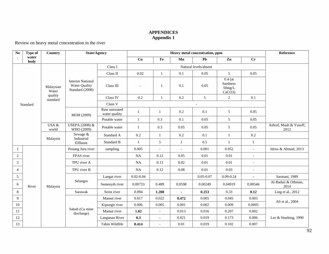
92

APPENDICES

Appendix 1

Review on heavy metal concentration in the river

No

.

Type of

water

body

Country State/Agency Heavy metal concentration, ppm Reference

Cu Fe Mn Pb Zn Cr

Standard

Malaysian

Water

quality

standard

Interim National

Water Quality

Standard (2008)

Class I Natural levels/absent

Class II 0.02 1 0.1 0.05 5 0.05

Class III - 1 0.1 0.05

0.4 (at

hardness

50mg/L

CaCO3)

Class IV 0.2 1 0.2 5 2 0.1

Class V -

MOH (2009)

Raw untreated

water quality 1 1 0.2 0.1 5 0.05

Potable water 1 0.3 0.1 0.05 5 0.05

USA &

world

USEPA (2008) &

WHO (2009) Potable water 1 0.3 0.05 0.05 5 0.05

Ashraf, Maah & Yusoff,

2012

Malaysia

Sewage &

Industrial

Effluent

Standard A 0.2 1 0.2 0.1 1 0.2

Standard B 1 5 1 0.5 1 1

1

River Malaysia

Penang Juru river sampling 0.005 - - 0.001 0.052 - Idriss & Ahmad, 2013

2 FPAS river

NA 0.12 0.05 0.01 0.01 -

3 TPU river A

NA 0.13 0.02 0.01 0.01 -

4 TPU river B

NA 0.12 0.08 0.01 0.03 -

5

Selangor

Langat river 0.02-0.04

0.05-0.07 0.09-0.24 - Sarmani, 1989

6 Semenyih river 0.00733 0.489 0.0598 0.00249 0.04919 0.00546 Al-Badaii & Othman,

2014

8 Sarawak Serin river 0.094 1.208 - 0.253 0.33 0.12 Ling et al., 2012

9

Sabah (Cu mine

discharge)

Mamut river 0.017 0.022 0.472 0.005 0.045 0.003 Ali et al., 2004

10 Kipungit river 0.006 0.005 0.001 0.002 0.009 0.0005

11 Mamut river 1.02 - 0.013 0.016 0.207 0.002

Lee & Stuebing, 1990 12 Langanan River 0.3 - 0.021 0.019 0.173 0.006

13 Tabin Wildlife 0.414 - 0.01 0.019 0.102 0.007

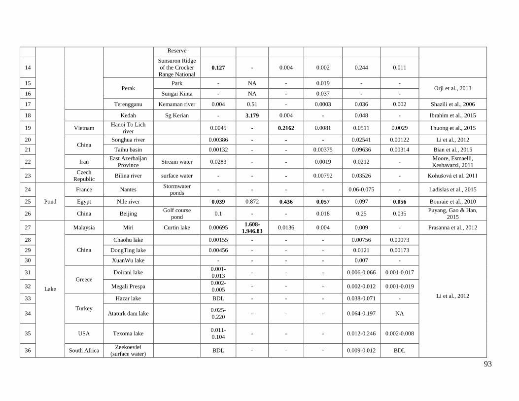
93

Reserve

14

Sunsuron Ridge

of the Crocker

Range National 0.127 - 0.004 0.002 0.244 0.011

15 Perak

Park - NA - 0.019 - - Orji et al., 2013

16 Sungai Kinta - NA - 0.037 - -

17 Terengganu Kemaman river 0.004 0.51 - 0.0003 0.036 0.002 Shazili et al., 2006

18

Kedah Sg Kerian - 3.179 0.004 - 0.048 - Ibrahim et al., 2015

19 Vietnam Hanoi To Lich

river 0.0045 - 0.2162 0.0081 0.0511 0.0029 Thuong et al., 2015

20 China

Songhua river

0.00386 - - - 0.02541 0.00122 Li et al., 2012

21 Taihu basin

0.00132 - - 0.00375 0.09636 0.00314 Bian et al., 2015

22 Iran East Azerbaijan

Province Stream water 0.0283 - - 0.0019 0.0212 -

Moore, Esmaelli,

Keshavarzi, 2011

23 Czech

Republic Bilina river surface water - - - 0.00792 0.03526 - Kohušová et al. 2011

24

Pond

France Nantes Stormwater

ponds - - - - 0.06-0.075 - Ladislas et al., 2015

25 Egypt Nile river

0.039 0.872 0.436 0.057 0.097 0.056 Bouraie et al., 2010

26 China Beijing Golf course

pond 0.1 - - 0.018 0.25 0.035

Puyang, Gao & Han,

2015

27

Lake

Malaysia Miri Curtin lake 0.00695 1.608-

1.946.83 0.0136 0.004 0.009 - Prasanna et al., 2012

28

China

Chaohu lake

0.00155 - - - 0.00756 0.00073

Li et al., 2012

29 DongTing lake

0.00456 - - - 0.0121 0.00173

30 XuanWu lake

- - - - 0.007 -

31

Greece

Doirani lake

0.001-

0.013 - - - 0.006-0.066 0.001-0.017

32 Megali Prespa

0.002-

0.005 - - - 0.002-0.012 0.001-0.019

33

Turkey

Hazar lake

BDL - - - 0.038-0.071 -

34 Ataturk dam lake

0.025-

0.220 - - - 0.064-0.197 NA

35 USA Texoma lake

0.011-

0.104 - - - 0.012-0.246 0.002-0.008

36 South Africa Zeekoevlei

(surface water) BDL - - - 0.009-0.012 BDL

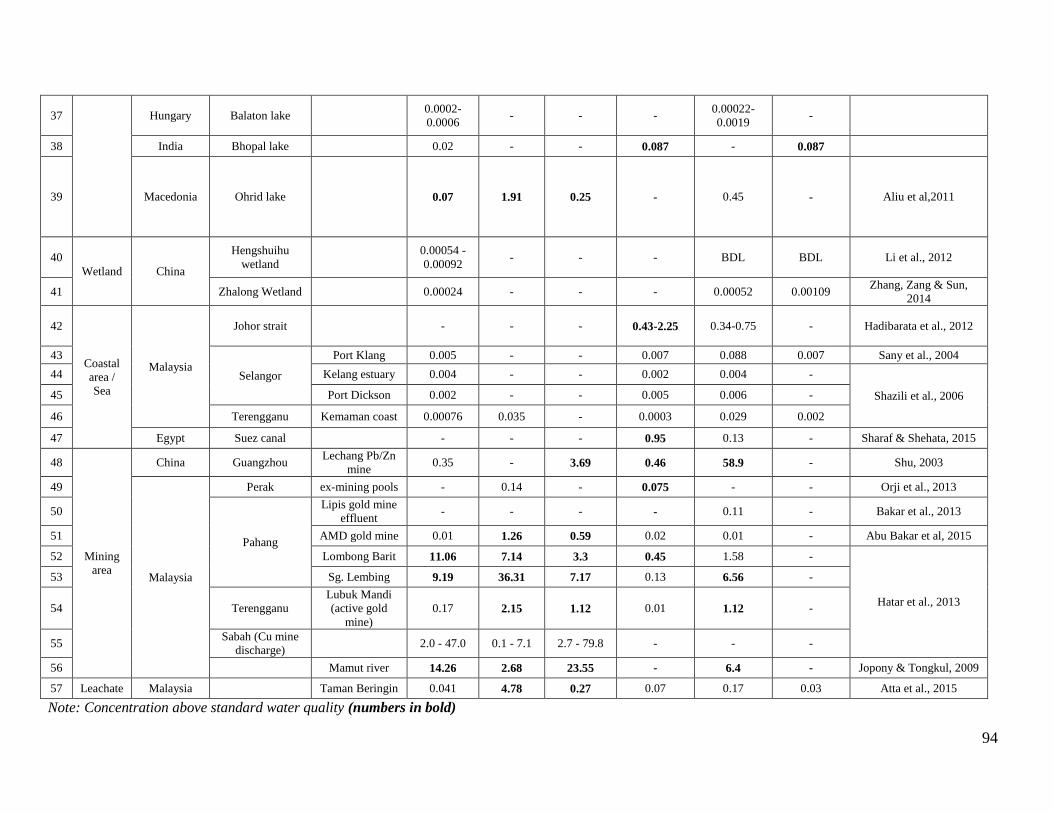
94

37 Hungary Balaton lake

0.0002-

0.0006 - - -

0.00022-

0.0019 -

38 India Bhopal lake

0.02 - - 0.087 - 0.087

39 Macedonia Ohrid lake

0.07 1.91 0.25 - 0.45 - Aliu et al,2011

40

Wetland China

Hengshuihu

wetland

0.00054 -

0.00092 - - - BDL BDL Li et al., 2012

41 Zhalong Wetland

0.00024 - - - 0.00052 0.00109 Zhang, Zang & Sun,

2014

42

Coastal

area /

Sea

Malaysia

Johor strait

- - - 0.43-2.25 0.34-0.75 - Hadibarata et al., 2012

43

Selangor

Port Klang 0.005 - - 0.007 0.088 0.007 Sany et al., 2004

44 Kelang estuary 0.004 - - 0.002 0.004 -

Shazili et al., 2006 45 Port Dickson 0.002 - - 0.005 0.006 -

46 Terengganu Kemaman coast 0.00076 0.035 - 0.0003 0.029 0.002

47 Egypt Suez canal

- - - 0.95 0.13 - Sharaf & Shehata, 2015

48

Mining

area

China Guangzhou Lechang Pb/Zn

mine 0.35 - 3.69 0.46 58.9 - Shu, 2003

49

Malaysia

Perak ex-mining pools - 0.14 - 0.075 - - Orji et al., 2013

50

Pahang

Lipis gold mine

effluent - - - - 0.11 - Bakar et al., 2013

51 AMD gold mine 0.01 1.26 0.59 0.02 0.01 - Abu Bakar et al, 2015

52 Lombong Barit 11.06 7.14 3.3 0.45 1.58 -

Hatar et al., 2013

53 Sg. Lembing 9.19 36.31 7.17 0.13 6.56 -

54 Terengganu

Lubuk Mandi

(active gold

mine)

0.17 2.15 1.12 0.01 1.12 -

55 Sabah (Cu mine

discharge) 2.0 - 47.0 0.1 - 7.1 2.7 - 79.8 - - -

56

Mamut river 14.26 2.68 23.55 - 6.4 - Jopony & Tongkul, 2009

57 Leachate Malaysia

Taman Beringin 0.041 4.78 0.27 0.07 0.17 0.03 Atta et al., 2015

Note: Concentration above standard water quality (numbers in bold)

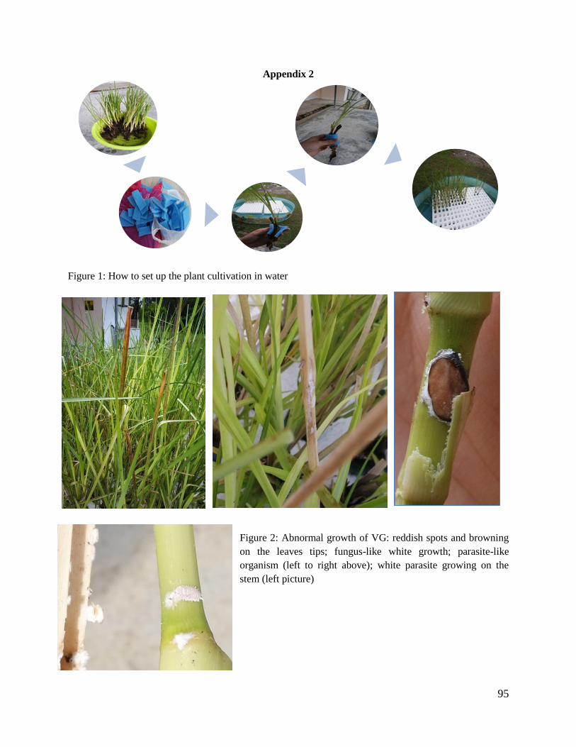
95

Appendix 2

Figure 1: How to set up the plant cultivation in water

Figure 2: Abnormal growth of VG: reddish spots and browning

on the leaves tips; fungus-like white growth; parasite-like

organism (left to right above); white parasite growing on the

stem (left picture)

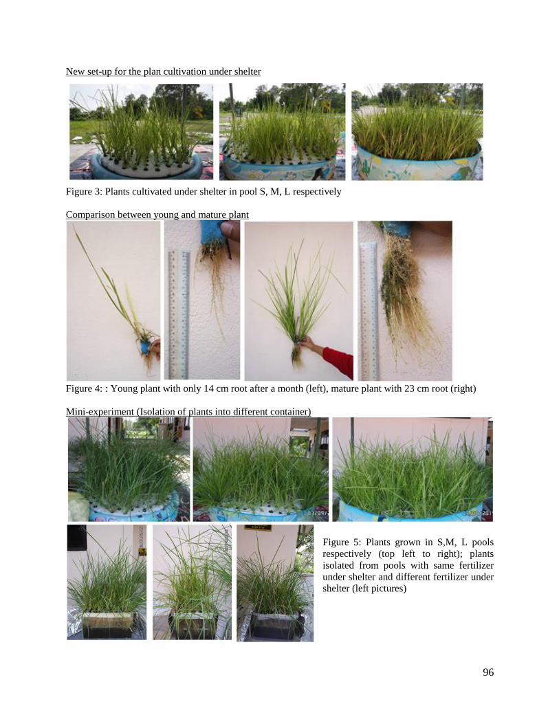
96

New set-up for the plan cultivation under shelter

Figure 3: Plants cultivated under shelter in pool S, M, L respectively

Comparison between young and mature plant

Figure 4: : Young plant with only 14 cm root after a month (left), mature plant with 23 cm root (right)

Mini-experiment (Isolation of plants into different container)

Figure 5: Plants grown in S,M, L pools

respectively (top left to right); plants

isolated from pools with same fertilizer

under shelter and different fertilizer under

shelter (left pictures)

97

Appendix 3

Setting high and low concentration

Option 1

Element Concentration, ppm River levels Reference

Low High

Cu 5 15 9.19 1Hatar et al., 2013

AIP Conference

Proceedings 1571,

641 (2013); doi:

10.1063/1.4858727

Fe 20 60 36.31

Mn 4 12 7.17

Pb 0.5 1.5 0.13

Zn 3.5 10.5 6.56

Appox 50% of river

level

Appox 150% of

river level

Sungai Lembing,

Pahang

Using one river as reference (the worst case scenario)

Option 2

Element Concentration, ppm River levels Reference

Low High

Cu 5 15 9.19 1Hatar et al., 2013

AIP Conference

Proceedings 1571, 641

(2013); doi:

10.1063/1.4858727

Fe 20 60 36.31

Mn 4 12 7.17

Pb 1.5 4.5 2.25 2Hadibarata et al., 2012

Zn 3.5 10.5 6.56 1

Appox 50% of river

level

Appox 150% of

river level

Sungai Lembing,

Pahang

All use one reference (worst case scenario), except Pb as it has the highest Pb concentration from my

read-ups.

Option 3

Element Low Concentration High Concentration

Reported Suggested Reference Reported Suggestion Reference

Cu 1.7519 2.0 9.19 10 1

Fe 3.876 2.0 36.31 40

Mn 2.1614 2.5 7.17 8

Pb 0.04589 0.5 2.25 2.5 2

Zn 0.6889 1.0 6.56 7 1

Average of the

river concentration from my read-ups

The worst case

scenario

For low concentration, I have averaged all the river concentration all over Malaysia to get the low

concentration. Is it relevant to do so?

For the high concentration, I used the one in Option 2.

Option 4

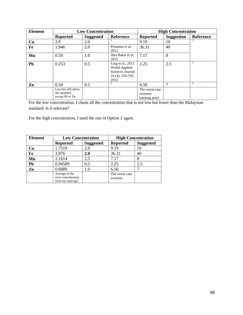
98

Element Low Concentration High Concentration

Reported Suggested Reference Reported Suggestion Reference

Cu 2.0 2.0 1

9.19 10 1

Fe 1.946 2.0 Prasanna et al.,

2012 36.31 40

Mn 0.59 1.0 Abu Bakar et al,

2015 7.17 8

Pb 0.253 0.5 Ling et al., 2012

World Applied

Sciences Journal

16 (4): 550-559,

2012

2.25 2.5 2

Zn 0.34 0.5 2

6.56 7 1

Low but still above

the standard, except Pb or Zn

The worst case

scenario

(mining area)

For the low concentration, I chose all the concentration that is not low but lower than the Malaysian

standard. Is it relevant?

For the high concentration, I used the one in Option 2 again.

Element Low Concentration High Concentration

Reported Suggested Reported Suggested

Cu 1.7519 2.0 9.19 10

Fe 3.876 2.0 36.31 40

Mn 2.1614 2.5 7.17 8

Pb 0.04589 0.5 2.25 2.5

Zn 0.6889 1.0 6.56 7

Average of the

river concentration from my read-ups

The worst case

scenario

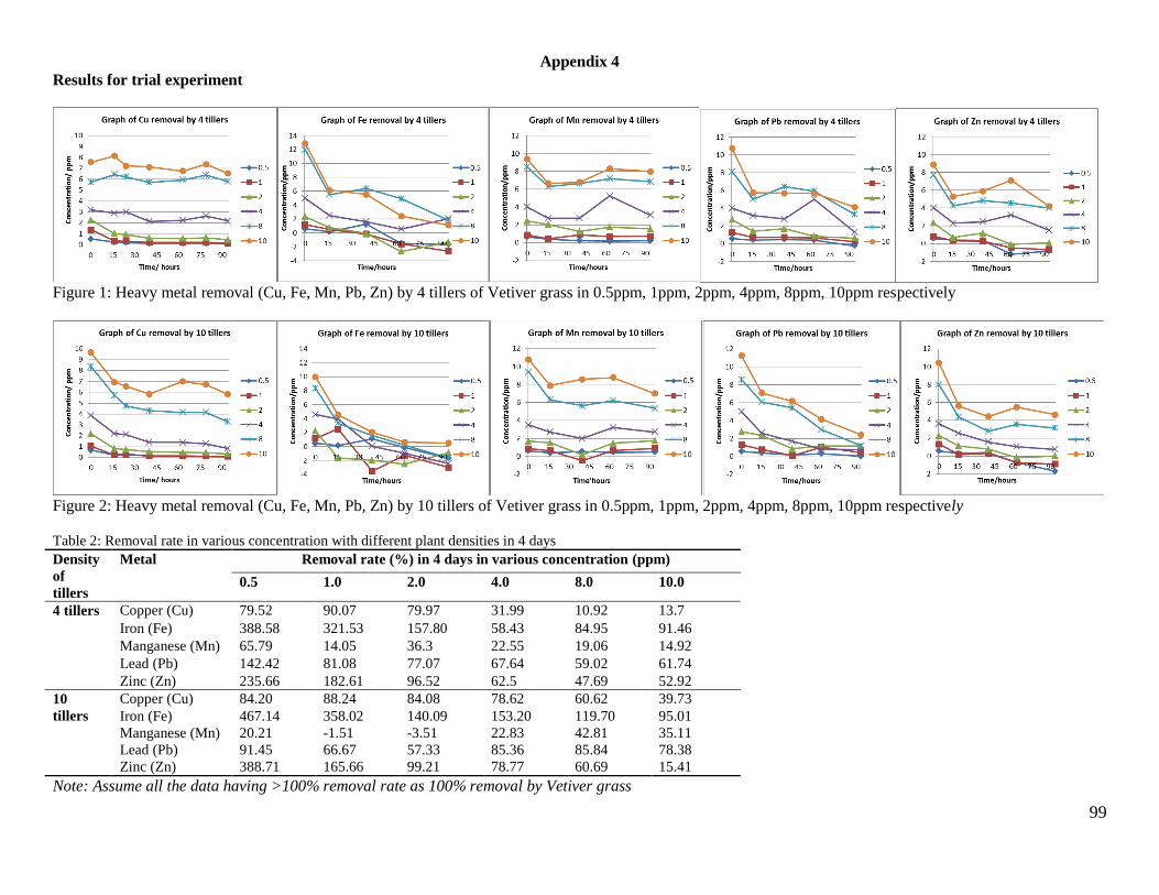
99

Appendix 4

Results for trial experiment

Figure 1: Heavy metal removal (Cu, Fe, Mn, Pb, Zn) by 4 tillers of Vetiver grass in 0.5ppm, 1ppm, 2ppm, 4ppm, 8ppm, 10ppm respectively

Figure 2: Heavy metal removal (Cu, Fe, Mn, Pb, Zn) by 10 tillers of Vetiver grass in 0.5ppm, 1ppm, 2ppm, 4ppm, 8ppm, 10ppm respectively

Table 2: Removal rate in various concentration with different plant densities in 4 days

Density

of

tillers

Metal Removal rate (%) in 4 days in various concentration (ppm)

0.5 1.0 2.0 4.0 8.0 10.0

4 tillers Copper (Cu) 79.52 90.07 79.97 31.99 10.92 13.7

Iron (Fe) 388.58 321.53 157.80 58.43 84.95 91.46

Manganese (Mn) 65.79 14.05 36.3 22.55 19.06 14.92

Lead (Pb) 142.42 81.08 77.07 67.64 59.02 61.74

Zinc (Zn) 235.66 182.61 96.52 62.5 47.69 52.92

10

tillers

Copper (Cu) 84.20 88.24 84.08 78.62 60.62 39.73

Iron (Fe) 467.14 358.02 140.09 153.20 119.70 95.01

Manganese (Mn) 20.21 -1.51 -3.51 22.83 42.81 35.11

Lead (Pb) 91.45 66.67 57.33 85.36 85.84 78.38

Zinc (Zn) 388.71 165.66 99.21 78.77 60.69 15.41

Note: Assume all the data having >100% removal rate as 100% removal by Vetiver grass

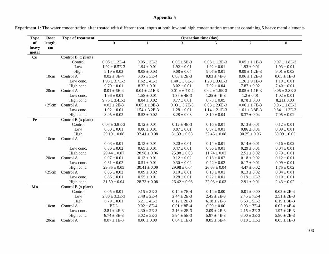
100

Appendix 5

Experiment 1: The water concentration after treated with different root length at both low and high concentration treatment containing 5 heavy metal elements

Type

of

heavy

metal

Root

length,

cm

Type of treatment

Operation time (day)

0 1 3 5 7 10

Cu Control B (x plant)

Control 0.05 ± 1.2E-4 0.05 ± 3E-3 0.03 ± 5E-3 0.03 ± 1.3E-3 0.05 ± 1.1E-3 0.07 ± 1.8E-3

Low 1.92 ± 8.5E-3 1.94 ± 0.01 1.92 ± 0.01 1.92 ± 0.01 1.93 ± 0.01 1.93 ± 0.01

High 9.19 ± 0.03 9.08 ± 0.03 9.08 ± 0.04 9.07 ± 0.01 9.09 ± 1.2E-3 9.01 ± 0.03

10cm Control A 0.02 ± 8E-4 0.05 ± 5E-4 0.03 ± 2E-3 0.03 ± 4E-3 0.06 ± 1.2E-3 0.05 ± 1E-3

Low conc. 1.93 ± 3.7E-3 1.62 ± 4E-3 1.40 ± 3.8E-3 1.28 ± 3.6E-3 1.26 ± 9.1E-3 1.10 ± 0.01

High conc. 9.70 ± 0.01 8.32 ± 0.01 8.02 ± 0.01 7.92 ± 0.04 7.87 ± 0.02 7.40 ± 0.01

20cm Control A 0.01 ± 6E-4 0.04 ± 2.1E-3 0.01 ± 6.7E-4 0.02 ± 1.5E-3 0.05 ± 1.1E-3 0.05 ± 2.8E-3

Low conc. 1.96 ± 0.01 1.58 ± 0.01 1.37 ± 4E-3 1.25 ± 4E-3 1.2 ± 0.01 1.02 ± 0.01

High conc. 9.75 ± 3.4E-3 8.84 ± 0.02 8.77 ± 0.01 8.73 ± 0.05 8.78 ± 0.03 8.21± 0.03

>25cm Control A 0.02 ± 2E-3 0.05 ± 1.9E-3 0.03 ± 3.2E-3 0.03 ± 2.6E-3 0.06 ± 1.7E-3 0.06 ± 1.8E-3

Low conc. 1.92 ± 0.01 1.54 ± 3.2E-3 1.28 ± 0.01 1.14 ± 2.1E-3 1.01 ± 3.8E-3 0.84 ± 1.3E-3

High conc. 8.95 ± 0.02 8.53 ± 0.02 8.28 ± 0.03 8.19 ± 0.04 8.37 ± 0.04 7.95 ± 0.02

Fe Control B (x plant)

Control 0.03 ± 3.8E-3 0.12 ± 0.01 0.12 ± 4E-3 0.16 ± 0.01 0.13 ± 0.01 0.12 ± 0.01

Low 0.80 ± 0.01 0.86 ± 0.01 0.87 ± 0.01 0.87 ± 0.01 0.86 ± 0.01 0.89 ± 0.01

High 29.19 ± 0.08 32.41 ± 0.08 31.33 ± 0.08 32.46 ± 0.08 30.25 ± 0.06 30.09 ± 0.03

10cm Control A

0.08 ± 0.01

0.13 ± 0.01

0.20 ± 0.01

0.14 ± 0.01

0.14 ± 0.01

0.16 ± 0.02

Low conc. 0.86 ± 0.02 0.65 ± 0.01 0.47 ± 0.01 0.36 ± 0.01 0.29 ± 0.01 0.04 ± 0.01

High conc. 29.44 ± 0.07 28.98 ± 0.06 25.98 ± 0.03 11.74 ± 0.03 2.51 ± 0.02 0.79 ± 0.01

20cm Control A 0.07 ± 0.01 0.13 ± 0.01 0.12 ± 0.02 0.13 ± 0.02 0.18 ± 0.02 0.12 ± 0.01

Low conc. 0.81 ± 0.02 0.51 ± 0.01 0.30 ± 0.02 0.22 ± 0.02 0.17 ± 0.01 0.09 ± 0.01

High conc. 29.85 ± 0.05 30.41 ± 0.09 29.98 ± 0.04 26.63 ± 0.04 4.47 ± 0.02 1.75 ± 0.02

>25cm Control A 0.05 ± 0.02 0.09 ± 0.02 0.10 ± 0.01 0.13 ± 0.01 0.13 ± 0.02 0.04 ± 0.01

Low conc. 0.85 ± 0.01 0.55 ± 0.01 0.28 ± 0.01 0.22 ± 0.01 0.18 ± 1E-3 0.10 ± 0.01

High conc. 31.59 ± 0.04 28.73 ± 0.08 26.42 ± 0.08 22.08 ± 0.03 2.91 ± 0.01 2.43 ± 0.02

Mn Control B (x plant)

Control 0.05 ± 0.01 0.15 ± 3E-3 0.14 ± 7E-4 0.14 ± 0.00 0.01 ± 0.00 0.03 ± 2E-4

Low 2.80 ± 3.2E-3 2.48 ± 2E-4 2.44 ± 2E-3 2.45 ± 2E-3 2.45 ± 7E-4 2.51 ± 2E-3

High 6.79 ± 0.01 6.21 ± 4E-3 6.12 ± 2E-3 6.18 ± 2E-3 6.63 ± 5E-3 6.19 ± 3E-3

10cm Control A BDL 0.02 ± 8E-4 0.01 ± 8E-4 0.00 ± 0.00 0.03 ± 7E-4 0.02 ± 4E-4

Low conc. 2.81 ± 4E-3 2.30 ± 2E-3 2.16 ± 2E-3 2.09 ± 2E-3 2.15 ± 2E-3 1.97 ± 2E-3

High conc. 6.74 ± 8E-3 6.02 ± 5E-3 5.94 ± 5E-3 5.97 ± 4E-3 6.00 ± 3E-3 5.80 ± 2E-3

20cm Control A 0.07 ± 1E-3 0.00 ± 0.00 0.04 ± 1E-3 0.05 ± 6E-4 0.10 ± 1E-3 0.05 ± 1E-3

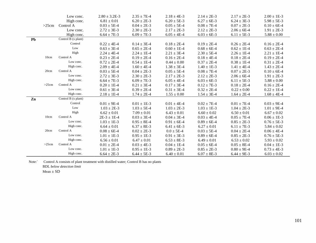
101

Note:` Control A consists of plant treatment with distilled water; Control B has no plants

BDL below detection limit

Mean ± SD

Low conc. 2.80 ± 3.2E-3 2.35 ± 7E-4 2.18 ± 4E-3 2.14 ± 2E-3 2.17 ± 2E-3 2.00 ± 1E-3

High conc. 6.81 ± 0.01 6.20 ± 2E-3 6.20 ± 5E-3 6.27 ± 6E-3 6.24 ± 3E-3 5.98 ± 5E-3

>25cm Control A 0.03 ± 5E-4 0.04 ± 2E-3 0.05 ± 5E-4 0.08 ± 7E-4 0.07 ± 2E-3 0.10 ± 6E-4

Low conc. 2.72 ± 3E-3 2.30 ± 2E-3 2.17 ± 2E-3 2.12 ± 2E-3 2.06 ± 6E-4 1.91 ± 2E-3

High conc. 6.64 ± 7E-3 6.09 ± 7E-3 6.05 ± 4E-4 6.03 ± 6E-3 6.11 ± 5E-3 5.88 ± 0.00

Pb Control B (x plant) Control 0.22 ± 4E-4 0.14 ± 3E-4 0.18 ± 2E-4 0.19 ± 2E-4 0.26 ± 2E-4 0.16 ± 2E-4

Low 0.63 ± 3E-4 0.65 ± 2E-4 0.60 ± 1E-4 0.68 ± 6E-4 0.62 ± 1E-4 0.63 ± 2E-4 High 2.24 ± 4E-4 2.24 ± 1E-4 2.21 ± 3E-4 2.30 ± 5E-4 2.26 ± 1E-4 2.21 ± 1E-4

10cm Control A 0.23 ± 2E-4 0.19 ± 2E-4 0.16 ± 2E-4 0.18 ± 4E-4 0.18 ± 2E-4 0.19 ± 2E-4 Low conc. 0.72 ± 2E-4 0.54 ± 1E-4 0.44 ± 0.00 0.37 ± 2E-4 0.38 ± 1E-4 0.31 ± 2E-4 High conc. 2.09 ± 4E-4 1.60 ± 4E-4 1.38 ± 3E-4 1.40 ± 1E-3 1.41 ± 4E-4 1.43 ± 2E-4

20cm Control A 0.03 ± 5E-4 0.04 ± 2E-3 0.05 ± 5E-4 0.08 ± 7E-4 0.07 ± 2E-3 0.10 ± 6E-4 Low conc. 2.72 ± 3E-3 2.30 ± 2E-3 2.17 ± 2E-3 2.12 ± 2E-3 2.06 ± 6E-4 1.91 ± 2E-3 High conc. 6.64 ± 7E-3 6.09 ± 7E-3 6.05 ± 4E-4 6.03 ± 6E-3 6.11 ± 5E-3 5.88 ± 0.00

>25cm Control A 0.20 ± 1E-4 0.21 ± 3E-4 0.17 ± 3E-4 0.12 ± 7E-3 0.18 ± 2E-4 0.16 ± 2E-4 Low conc. 0.61 ± 3E-4 0.39 ± 2E-4 0.31 ± 3E-4 0.32 ± 2E-4 0.22 ± 0.00 0.22 ± 1E-4 High conc. 2.18 ± 1E-4 1.74 ± 2E-4 1.55 ± 0.00 1.54 ± 3E-4 1.64 ± 2E-4 1.68 ± 4E-4

Zn Control B (x plant) Control 0.01 ± 9E-4 0.01 ± 1E-3 0.01 ± 4E-4 0.02 ± 7E-4 0.01 ± 7E-4 0.03 ± 9E-4

Low 1.03 ± 2E-3 1.03 ± 5E-4 1.03 ± 2E-3 1.03 ± 1E-3 1.04 ± 2E-3 1.01 ± 9E-4 High 6.62 ± 0.01 7.09 ± 0.01 6.43 ± 0.01 6.60 ± 0.02 6.50 ± 0.01 6.67 ± 0.02

10cm Control A 2E-3 ± 1E-4 0.03 ± 3E-4 0.04 ± 3E-4 0.03 ± 4E-4 0.05 ± 7E-4 0.06 ± 1E-3 Low conc. 1.03 ± 1E-3 0.95 ± 8E-4 0.91 ± 6E-4 0.89 ± 6E-4 0.85 ± 2E-3 0.76 ± 5E-3 High conc. 6.64 ± 0.01 6.37 ± 8E-3 6.41 ± 6E-3 6.27 ± 0.01 6.11 ± 7E-3 5.84 ± 0.02

20cm Control A 0.08 ± 6E-4 0.02 ± 2E-3 0.0 ± 5E-4 0.03 ± 5E-4 0.04 ± 2E-4 0.06 ± 4E-4 Low conc. 1.01 ± 1E-3 0.95 ± 1E-3 0.91 ± 3E-3 0.89 ± 6E-4 0.85 ± 2E-3 0.76 ± 5E-3 High conc. 6.56 ± 0.01 6.47 ± 0.01 6.53 ± 8E-3 6.49 ± 0.01 6.53 ± 0.02 5.93 ± 0.02

>25cm Control A 0.01 ± 2E-4 0.03 ± 4E-3 0.04 ± 1E-4 0.05 ± 6E-4 0.05 ± 8E-4 0.04 ± 1E-3 Low conc. 1.01 ± 1E-3 0.95 ± 1E-3 0.89 ± 2E-3 0.85 ± 2E-3 0.80 ± 9E-4 0.73 ± 4E-3 High conc. 6.64 ± 2E-3 6.44 ± 5E-3 6.40 ± 0.01 6.07 ± 8E-3 6.44 ± 9E-3 6.03 ± 0.02

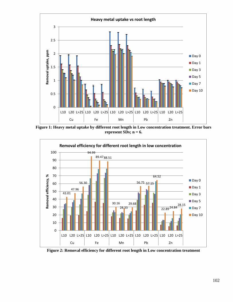
102

Figure 1: Heavy metal uptake by different root length in Low concentration treatment. Error bars

represent SDs; n = 6.

Figure 2: Removal efficiency for different root length in Low concentration treatment

0

0.5

1

1.5

2

2.5

3

L10 L20 L>25 L10 L20 L>25 L10 L20 L>25 L10 L20 L>25 L10 L20 L>25

Cu Fe Mn Pb Zn

Re

mo

val u

pta

ke, p

pm

Heavy metal uptake vs root length

Day 0

Day 1

Day 3

Day 5

Day 7

Day 10

43.01 47.96

56.30

94.99

89.47 88.51

30.16

28.33 29.68

56.75 57.15

64.52

22.89 24.84 28.15

0

10

20

30

40

50

60

70

80

90

100

L10 L20 L>25 L10 L20 L>25 L10 L20 L>25 L10 L20 L>25 L10 L20 L>25

Cu Fe Mn Pb Zn

Re

mo

val e

ffic

ien

cy,

%

Removal efficiency for different root length in low concentration

Day 0

Day 1

Day 3

Day 5

Day 7

Day 10

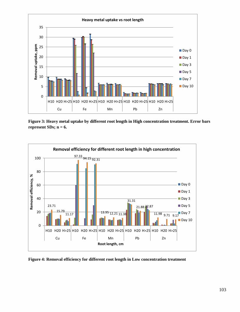
103

Figure 3: Heavy metal uptake by different root length in High concentration treatment. Error bars

represent SDs; n = 6.

Figure 4: Removal efficiency for different root length in Low concentration treatment

0

5

10

15

20

25

30

35

H10 H20 H>25 H10 H20 H>25 H10 H20 H>25 H10 H20 H>25 H10 H20 H>25

Cu Fe Mn Pb Zn

Re

mo

val u

pta

ke, p

pm

Heavy metal uptake vs root length

Day 0

Day 1

Day 3

Day 5

Day 7

Day 10

23.71

15.79 11.17

97.33 94.15 92.31

13.95 12.21 11.38

31.31

21.88 22.87

11.98 9.71 9.17

0

20

40

60

80

100

H10 H20 H>25 H10 H20 H>25 H10 H20 H>25 H10 H20 H>25 H10 H20 H>25

Cu Fe Mn Pb Zn

Re

mo

val e

ffic

ien

cy,

%

Root length, cm

Removal efficiency for different root length in high concentration

Day 0

Day 1

Day 3

Day 5

Day 7

Day 10

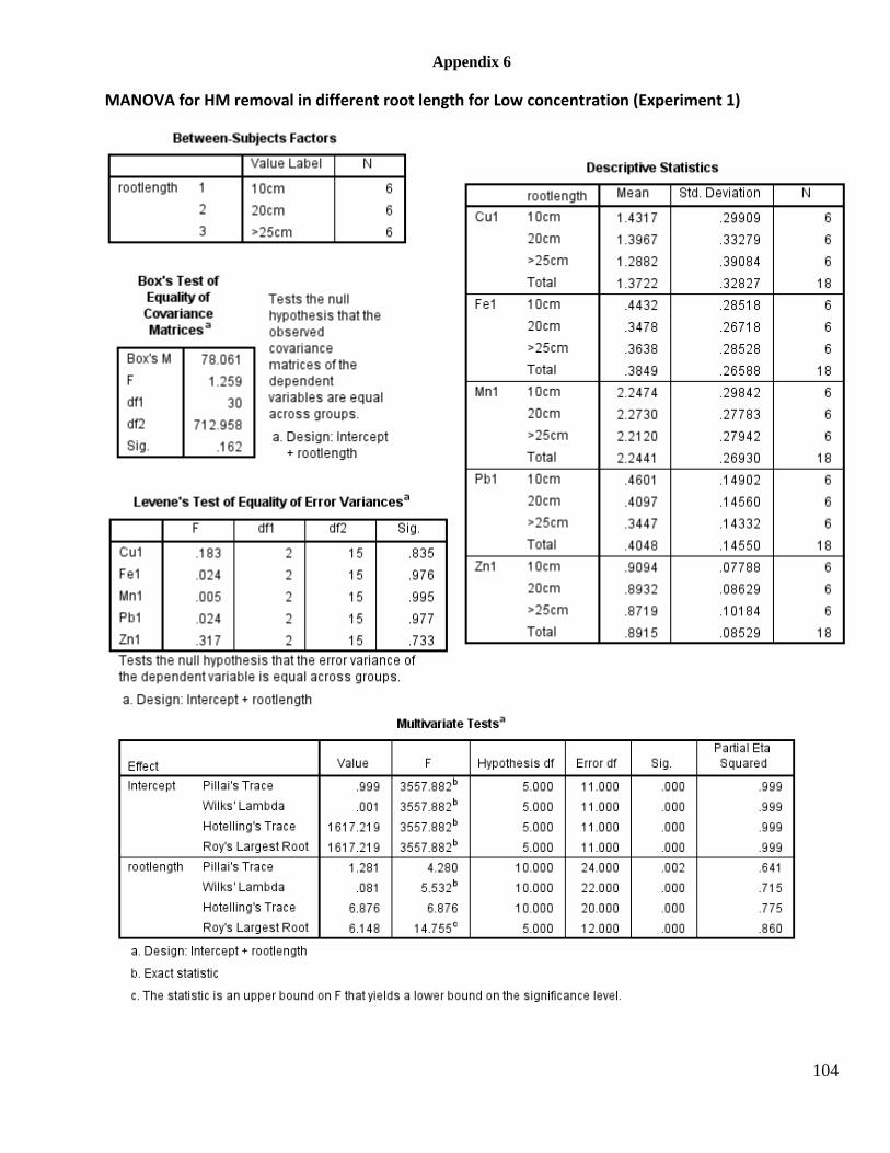
104

Appendix 6

MANOVA for HM removal in different root length for Low concentration (Experiment 1)

105

106

Appendix 7

Pearson product-moment Correlation Coefficient for Low concentration (Experiment 1)

Descriptive Statistics

Mean Std. Deviation N

rootlength 2.00 .840 18

Cu1 1.3722 .32827 18

Fe1 .3849 .26588 18

Mn1 2.2441 .26930 18

Pb1 .4048 .14550 18

Zn1 .8915 .08529 18

Correlations

rootlength Cu1 Fe1 Mn1 Pb1 Zn1

rootlength Pearson Correlation 1 -.184 -.125 -.055 -.333 -.185

Sig. (2-tailed) .466 .620 .827 .177 .463

N 18 18 18 18 18 18

Cu1 Pearson Correlation -.184 1 .967** .956

** .961

** .966

**

Sig. (2-tailed) .466 .000 .000 .000 .000

N 18 18 18 18 18 18

Fe1 Pearson Correlation -.125 .967** 1 .934

** .941

** .933

**

Sig. (2-tailed) .620 .000 .000 .000 .000

N 18 18 18 18 18 18

Mn1 Pearson Correlation -.055 .956** .934

** 1 .945

** .899

**

Sig. (2-tailed) .827 .000 .000 .000 .000

N 18 18 18 18 18 18

Pb1 Pearson Correlation -.333 .961** .941

** .945

** 1 .895

**

Sig. (2-tailed) .177 .000 .000 .000 .000

N 18 18 18 18 18 18

Zn1 Pearson Correlation -.185 .966** .933

** .899

** .895

** 1

Sig. (2-tailed) .463 .000 .000 .000 .000

N 18 18 18 18 18 18

107

Appendix 8

MANOVA for HM removal in different root length for High concentration (Experiment 1)

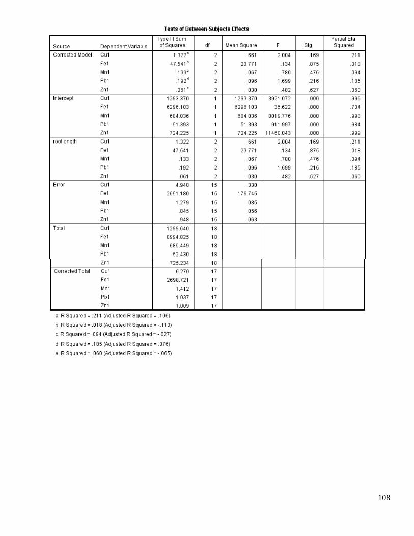
108

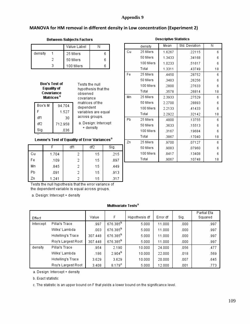
109

Appendix 9

MANOVA for HM removal in different density in Low concentration (Experiment 2)

110

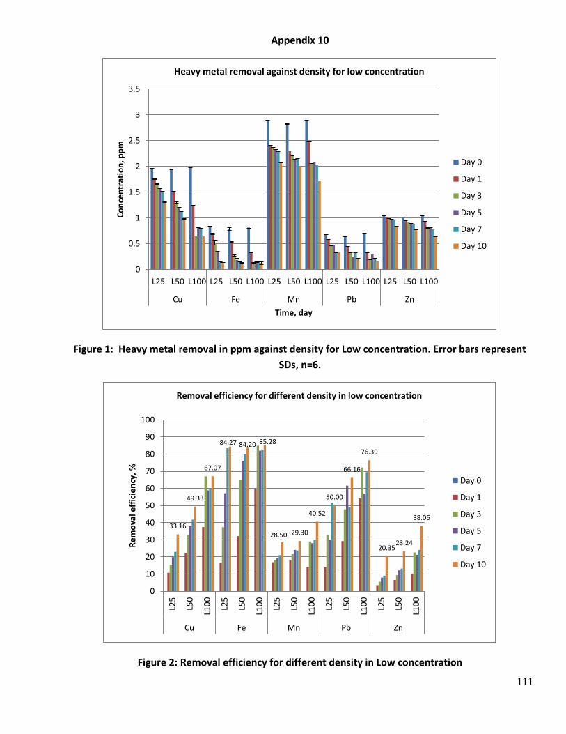
111

Appendix 10

Figure 1: Heavy metal removal in ppm against density for Low concentration. Error bars represent

SDs, n=6.

Figure 2: Removal efficiency for different density in Low concentration

0

0.5

1

1.5

2

2.5

3

3.5

L25 L50 L100 L25 L50 L100 L25 L50 L100 L25 L50 L100 L25 L50 L100

Cu Fe Mn Pb Zn

Co

nce

ntr

atio

n, p

pm

Time, day

Heavy metal removal against density for low concentration

Day 0

Day 1

Day 3

Day 5

Day 7

Day 10

33.16

49.33

67.07

84.27 84.20 85.28

28.50 29.30

40.52

50.00

66.16

76.39

20.35 23.24

38.06

0

10

20

30

40

50

60

70

80

90

100

L25

L50

L10

0

L25

L50

L10

0

L25

L50

L10

0

L25

L50

L10

0

L25

L50

L10

0

Cu Fe Mn Pb Zn

Re

mo

val e

ffic

ien

cy,

%

Removal efficiency for different density in low concentration

Day 0

Day 1

Day 3

Day 5

Day 7

Day 10

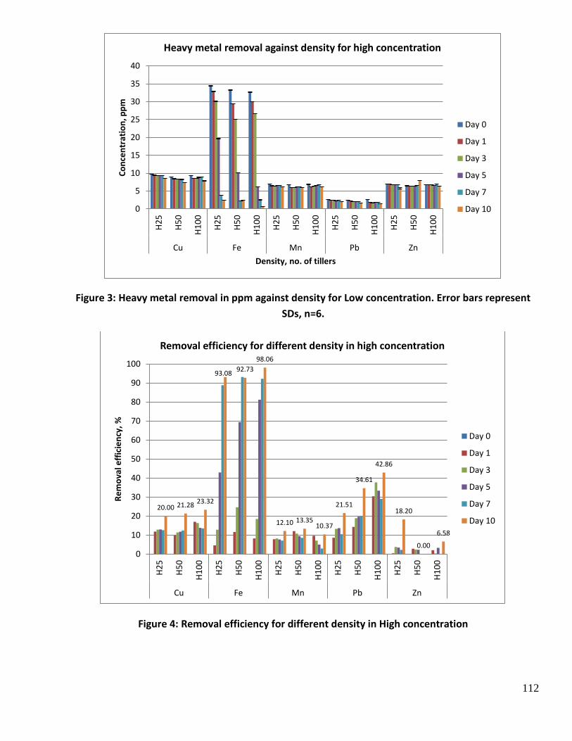
112

Figure 3: Heavy metal removal in ppm against density for Low concentration. Error bars represent

SDs, n=6.

Figure 4: Removal efficiency for different density in High concentration

0

5

10

15

20

25

30

35

40

H2

5

H5

0

H1

00

H2

5

H5

0

H1

00

H2

5

H5

0

H1

00

H2

5

H5

0

H1

00

H2

5

H5

0

H1

00

Cu Fe Mn Pb Zn

Co

nce

ntr

atio

n, p

pm

Density, no. of tillers

Heavy metal removal against density for high concentration

Day 0

Day 1

Day 3

Day 5

Day 7

Day 10

20.00 21.28 23.32

93.08 92.73

98.06

12.10 13.35 10.37

21.51

34.61

42.86

18.20

0.00

6.58

0

10

20

30

40

50

60

70

80

90

100

H2

5

H5

0

H1

00

H2

5

H5

0

H1

00

H2

5

H5

0

H1

00

H2

5

H5

0

H1

00

H2

5

H5

0

H1

00

Cu Fe Mn Pb Zn

Re

mo

val e

ffic

ien

cy,

%

Removal efficiency for different density in high concentration

Day 0

Day 1

Day 3

Day 5

Day 7

Day 10

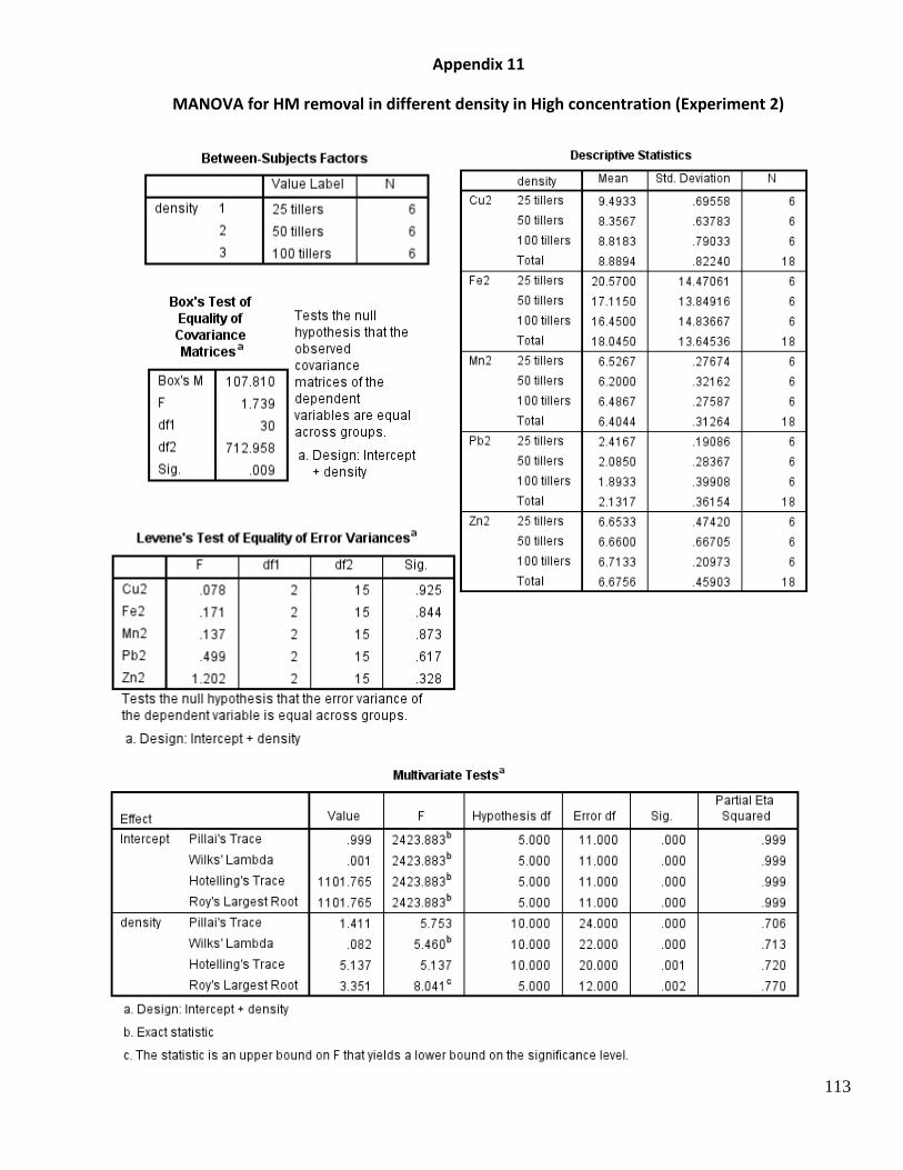
113

Appendix 11

MANOVA for HM removal in different density in High concentration (Experiment 2)

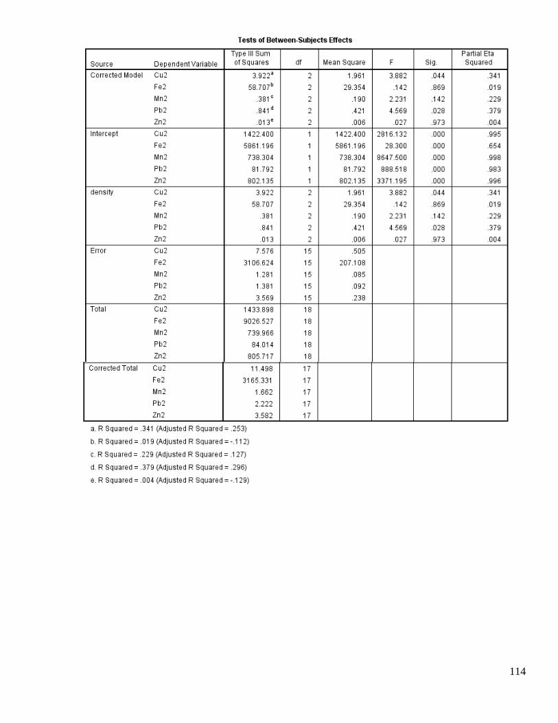
114

115

Appendix 12

T-test to compare each heavy metal between low and high concentration (Experiment 1)

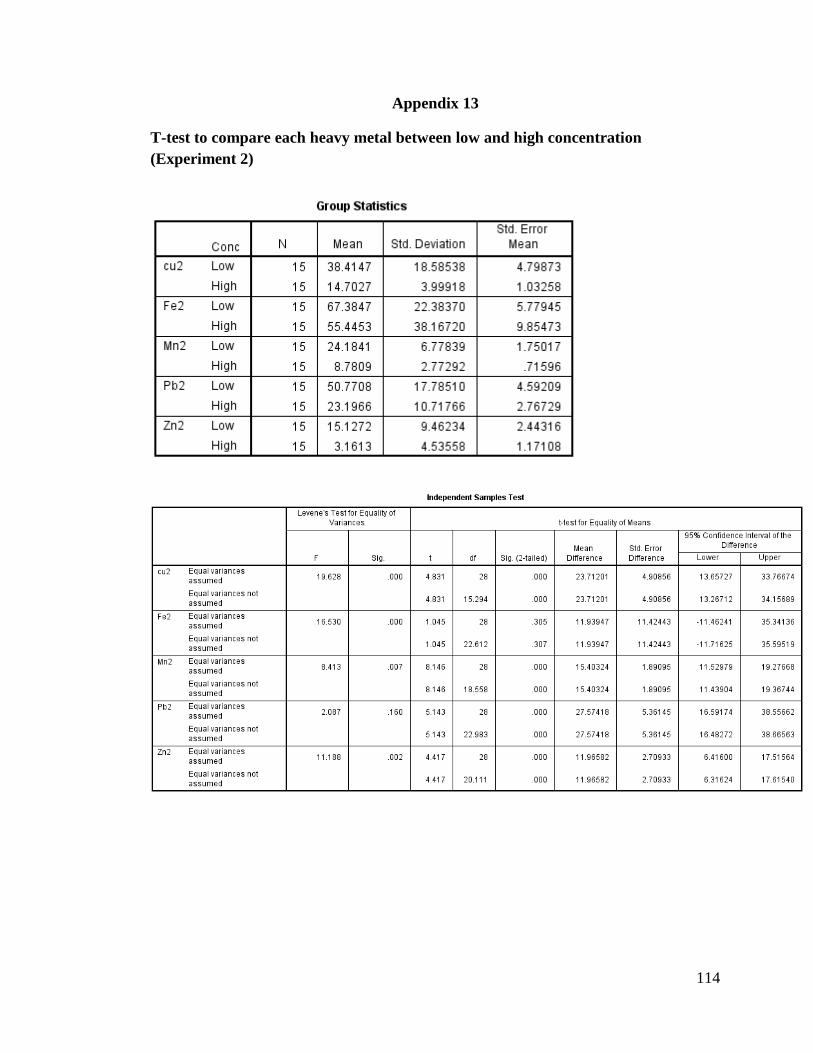
114

Appendix 13

T-test to compare each heavy metal between low and high concentration

(Experiment 2)

115

Appendix 14

Pearson product-moment correlation coefficient for heavy metal removal and

accumulation in root

116

Appendix 15

T-tests results for heavy metal accumulation in different plant part after 10 days for

Low concentration treatment

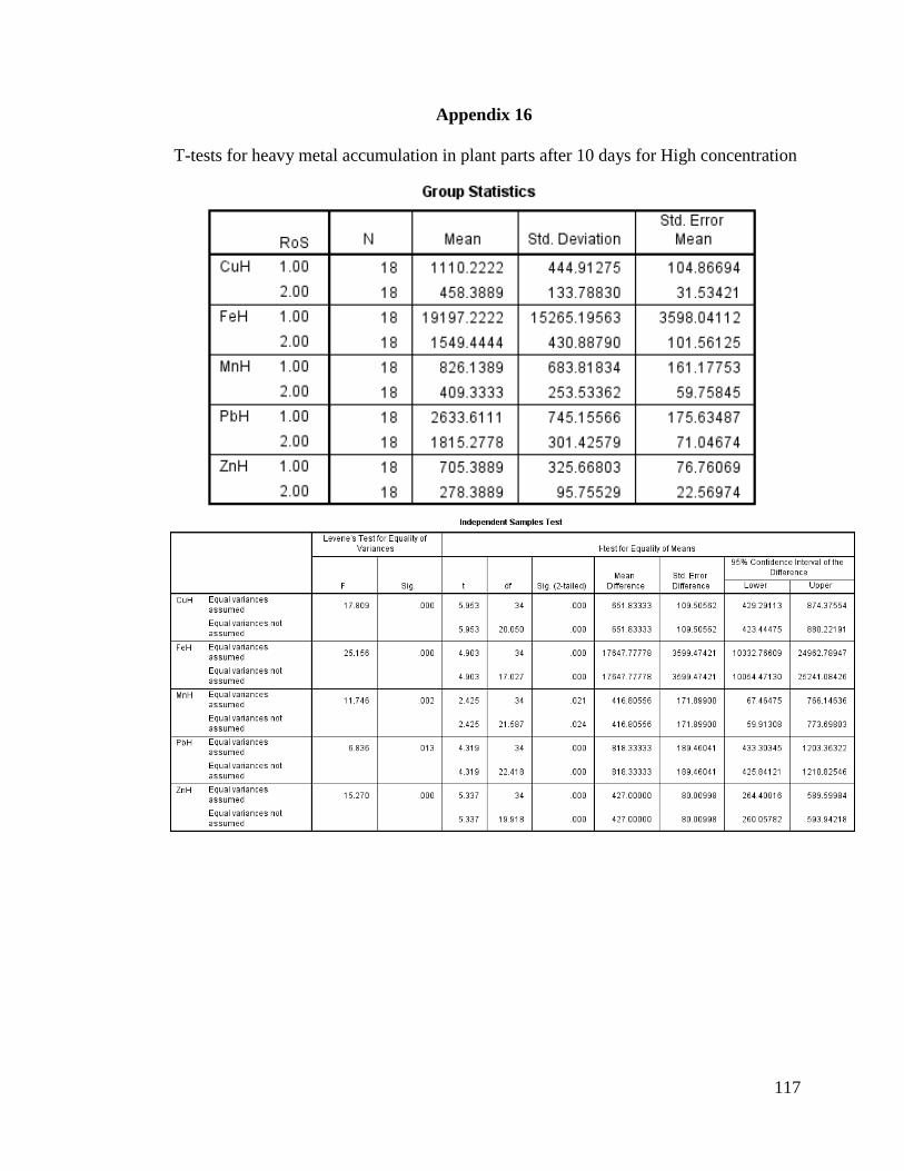
117

Appendix 16

T-tests for heavy metal accumulation in plant parts after 10 days for High concentration

118

Appendix 17

T-tests for heavy metal accumulation in plant root for different concentration

119

Appendix 18

T-tests for heavy metal accumulation in plant shoots for different concentration

120

BIODATA OF STUDENT

The author of this thesis, Ashton Lim Suelee was born on 4th

October 1992 in Kuching,

Sarawak. She lives in Kuching, but currently stays in UPM Serdang in pursuing her

Bachelor of Environmental Science and Technology. She is from an average family

consisting of her parents, an elder sister and a younger brother, in which their age gap is

only 14 months in average. Her parents both work together at her late-grandfather’s

forwarding agencies company called Natural Service Company – her father is the

company manager and her mother is working alongside with him.

She has completed her primary education from year 1999 to 2004 at Sekolah Rendah

Bantuan St. Theresa Padungan in Kuching, Sarawak. Then, she continued her secondary

education at Sekolah Menengah Kebangsaan St. Teresa Kuching (2005 – 2009) and

continued further till Form 6 at Sekolah Menengah Kebangsaan St. Joseph Kuching

(2010-2011). Currently, she furthers her study as an undergraduate student in UPM

eversince year 2012, whereby she would be graduating soon in year 2016.