PhysicsDepartment, TechnicalUniversityofDenmark ... · PhysicsDepartment,...

User and programmers guide

to the neutron ray-tracing package McStas,

version 2.0

P Willendrup, E Farhi, E Knudsen, U Filges, K Lefmann

Physics Department,

Technical University of Denmark, 2800 Kongens Lyngby, Denmark

November, 2012

nMcStas

Abstract

The software package McStas is a tool for carrying out Monte Carlo ray-tracingsimulations of neutron scattering instruments with high complexity and precision.The simulations can compute all aspects of the performance of instruments and canthus be used to optimize the use of existing equipment, design new instrumentation,and carry out virtual experiments for e.g. training, experimental planning or dataanalysis. McStas is based on a unique design where an automatic compilation processtranslates high-level textual instrument descriptions into efficient ANSI-C code. Thisdesign makes it simple to set up typical simulations and also gives essentially unlimitedfreedom to handle more unusual cases.

This report constitutes the reference manual for McStas, and, together with themanual for the McStas components, it contains documentation of most aspects ofthe program. It covers the various ways to compile and run simulations, a descrip-tion of the meta-language used to define simulations, and some example simulationsperformed with the program.

This report documents McStas version 2.0, released November, 2012

The authors are:

Peter Kjær Willendrup <[email protected]>

Physics Department, Technical University of Denmark, Kongens Lyngby, Den-mark

Emmanuel Farhi <[email protected]>Institut Laue-Langevin, Grenoble, France

Erik Knudsen <[email protected]>

Physics Department, Technical University of Denmark, Kongens Lyngby, Den-mark

Kim Lefmann <[email protected]>

Niels Bohr Institute, University of Copenhagen, Denmark

as well as authors who left the project:

Peter Christiansen <[email protected]>

Materials Research Department, Risø National Laboratory, Roskilde, DenmarkPresent address: University of Lund, Lund, SwedenKlaus Lieutenant <[email protected]>Institut Laue-Langevin, Grenoble, FrancePresent address: Helmotlz Zentrum Berlin, GermanyKristian Nielsen <[email protected]>

Materials Research Department, Risø National Laboratory, Roskilde, DenmarkPresently associated with: MySQL AB, Sweden

ISBN 978–87–550–3679–6ISSN 0106–2840

Information Service Department · Risø DTU · 2012

Contents

Preface and acknowledgements 7

1 Introduction to McStas 9

1.1 Development of Monte Carlo neutron simulation . . . . . . . . . . . . . . . 9

1.2 Scientific background . . . . . . . . . . . . . . . . . . . . . . . . . . . . . . . 10

1.2.1 The goals of McStas . . . . . . . . . . . . . . . . . . . . . . . . . . . 11

1.3 The design of McStas . . . . . . . . . . . . . . . . . . . . . . . . . . . . . . 12

1.4 Overview . . . . . . . . . . . . . . . . . . . . . . . . . . . . . . . . . . . . . 14

2 New features in McStas 2.0 15

2.1 Kernel . . . . . . . . . . . . . . . . . . . . . . . . . . . . . . . . . . . . . . . 15

2.2 Run-time . . . . . . . . . . . . . . . . . . . . . . . . . . . . . . . . . . . . . 15

2.3 Components and Library . . . . . . . . . . . . . . . . . . . . . . . . . . . . 16

2.3.1 Components . . . . . . . . . . . . . . . . . . . . . . . . . . . . . . . 16

2.3.2 New example instruments and Data files . . . . . . . . . . . . . . . . 16

2.4 Documentation . . . . . . . . . . . . . . . . . . . . . . . . . . . . . . . . . . 16

2.5 Tools, installation . . . . . . . . . . . . . . . . . . . . . . . . . . . . . . . . . 17

2.5.1 New tool features . . . . . . . . . . . . . . . . . . . . . . . . . . . . . 17

2.5.2 Platform support . . . . . . . . . . . . . . . . . . . . . . . . . . . . . 17

2.5.3 Various . . . . . . . . . . . . . . . . . . . . . . . . . . . . . . . . . . 17

2.5.4 Warnings . . . . . . . . . . . . . . . . . . . . . . . . . . . . . . . . . 18

2.6 Future extensions . . . . . . . . . . . . . . . . . . . . . . . . . . . . . . . . . 18

3 Installing McStas 19

3.1 Getting McStas . . . . . . . . . . . . . . . . . . . . . . . . . . . . . . . . . . 19

3.2 Licensing . . . . . . . . . . . . . . . . . . . . . . . . . . . . . . . . . . . . . 20

3.3 Installation on windows . . . . . . . . . . . . . . . . . . . . . . . . . . . . . 20

3.4 Installation on Unix systems . . . . . . . . . . . . . . . . . . . . . . . . . . . 20

3.4.1 Debian class systems . . . . . . . . . . . . . . . . . . . . . . . . . . . 21

3.4.2 Other Linux/Unix systems . . . . . . . . . . . . . . . . . . . . . . . 21

3.4.3 Configuration and installation . . . . . . . . . . . . . . . . . . . . . . 22

3.4.4 Specifying non-standard options . . . . . . . . . . . . . . . . . . . . 22

3.5 Finishing and Testing the McStas distribution . . . . . . . . . . . . . . . . . 23

DTU 3

4 Monte Carlo Techniques and simulation strategy 25

4.1 Neutron spectrometer simulations . . . . . . . . . . . . . . . . . . . . . . . . 25

4.1.1 Monte Carlo ray tracing simulations . . . . . . . . . . . . . . . . . . 25

4.2 The neutron weight . . . . . . . . . . . . . . . . . . . . . . . . . . . . . . . . 26

4.2.1 Statistical errors of non-integer counts . . . . . . . . . . . . . . . . . 26

4.3 Weight factor transformations during a Monte Carlo choice . . . . . . . . . 28

4.3.1 Direction focusing . . . . . . . . . . . . . . . . . . . . . . . . . . . . 28

4.4 Adaptive and Stratified sampling . . . . . . . . . . . . . . . . . . . . . . . . 28

4.5 Accuracy of Monte Carlo simulations . . . . . . . . . . . . . . . . . . . . . . 29

5 Running McStas 31

5.1 Brief introduction to the graphical user interface . . . . . . . . . . . . . . . 32

5.1.1 New releases of McStas . . . . . . . . . . . . . . . . . . . . . . . . . 35

5.2 Running the instrument compiler . . . . . . . . . . . . . . . . . . . . . . . . 35

5.2.1 Code generation options . . . . . . . . . . . . . . . . . . . . . . . . . 36

5.2.2 Specifying the location of files . . . . . . . . . . . . . . . . . . . . . . 36

5.2.3 Embedding the generated simulations in other programs . . . . . . . 37

5.2.4 Running the C compiler . . . . . . . . . . . . . . . . . . . . . . . . . 37

5.3 Running the simulations . . . . . . . . . . . . . . . . . . . . . . . . . . . . . 39

5.3.1 Choosing an output data file format . . . . . . . . . . . . . . . . . . 40

5.3.2 Basic import and plot of results . . . . . . . . . . . . . . . . . . . . . 40

5.3.3 Interacting with a running simulation . . . . . . . . . . . . . . . . . 41

5.3.4 Optimizing simulation speed . . . . . . . . . . . . . . . . . . . . . . 44

5.3.5 Optimizing instrument parameters . . . . . . . . . . . . . . . . . . . 45

5.4 Using simulation front-ends . . . . . . . . . . . . . . . . . . . . . . . . . . . 47

5.4.1 The graphical user interface (mcgui) . . . . . . . . . . . . . . . . . . 48

5.4.2 Running simulations on the commandline (mcrun) . . . . . . . . . . 53

5.4.3 Graphical display of simulations (mcdisplay) . . . . . . . . . . . . . 55

5.4.4 Plotting the results of a simulation (mcplot) . . . . . . . . . . . . . . 57

5.4.5 Plotting resolution functions (mcresplot) . . . . . . . . . . . . . . . . 58

5.4.6 Creating and viewing the library, component/instrument help andManuals (mcdoc) . . . . . . . . . . . . . . . . . . . . . . . . . . . . . 59

5.4.7 Translating McStas components for Vitess (mcstas2vitess) . . . . . . 59

5.4.8 Translating McStas results files between Matlab and Scilab formats 60

5.4.9 Translating and merging McStas results files (all text formats) . . . 60

5.5 Data formats - Analyzing and visualizing the simulation results . . . . . . . 61

5.5.1 McStas and PGPLOT format . . . . . . . . . . . . . . . . . . . . . . 61

5.5.2 Matlab, Scilab and IDL formats . . . . . . . . . . . . . . . . . . . . 62

5.5.3 HTML/VRML and XML formats . . . . . . . . . . . . . . . . . . . . 63

5.5.4 NeXus format . . . . . . . . . . . . . . . . . . . . . . . . . . . . . . . 63

5.6 Using computer Grids and Clusters . . . . . . . . . . . . . . . . . . . . . . . 64

5.6.1 Distribute mcrun simulations on grids, multi-cores and clusters (SSHgrid) . . . . . . . . . . . . . . . . . . . . . . . . . . . . . . . . . . . . 65

5.6.2 Parallel computing (MPI) . . . . . . . . . . . . . . . . . . . . . . . . 66

5.6.3 McRun script with MPI support (mpich) . . . . . . . . . . . . . . . 67

5.6.4 McStas/MPI Performance . . . . . . . . . . . . . . . . . . . . . . . . 68

4 DTU

5.6.5 MPI and Grid Bugs and limitations . . . . . . . . . . . . . . . . . . 69

6 The McStas kernel and meta-language 70

6.1 Notational conventions . . . . . . . . . . . . . . . . . . . . . . . . . . . . . . 71

6.2 Syntactical conventions . . . . . . . . . . . . . . . . . . . . . . . . . . . . . 72

6.3 Writing instrument definitions . . . . . . . . . . . . . . . . . . . . . . . . . . 74

6.3.1 The instrument definition head . . . . . . . . . . . . . . . . . . . . . 74

6.3.2 The DECLARE section . . . . . . . . . . . . . . . . . . . . . . . . . . . 75

6.3.3 The INITIALIZE section . . . . . . . . . . . . . . . . . . . . . . . . . 75

6.3.4 The NEXUS extension . . . . . . . . . . . . . . . . . . . . . . . . . . . 75

6.3.5 The TRACE section . . . . . . . . . . . . . . . . . . . . . . . . . . . . 76

6.3.6 The SAVE section . . . . . . . . . . . . . . . . . . . . . . . . . . . . . 78

6.3.7 The FINALLY section . . . . . . . . . . . . . . . . . . . . . . . . . . . 78

6.3.8 The end of the instrument definition . . . . . . . . . . . . . . . . . . 78

6.3.9 Code for the instrument vanadium example.instr . . . . . . . . . . 78

6.4 Writing instrument definitions - complex arrangements and syntax . . . . . 80

6.4.1 Embedding instruments in instruments TRACE . . . . . . . . . . . 81

6.4.2 Groups and component extensions - GROUP - EXTEND . . . . . . 81

6.4.3 Duplication of component instances - COPY . . . . . . . . . . . . . 82

6.4.4 Conditional components - WHEN . . . . . . . . . . . . . . . . . . . 84

6.4.5 Component loops and non sequential propagation - JUMP . . . . . . 85

6.4.6 Enhancing statistics reaching components - SPLIT . . . . . . . . . . 86

6.5 Writing component definitions . . . . . . . . . . . . . . . . . . . . . . . . . . 87

6.5.1 The component definition header . . . . . . . . . . . . . . . . . . . . 87

6.5.2 The DECLARE section . . . . . . . . . . . . . . . . . . . . . . . . . . . 89

6.5.3 The SHARE section . . . . . . . . . . . . . . . . . . . . . . . . . . . . 90

6.5.4 The INITIALIZE section . . . . . . . . . . . . . . . . . . . . . . . . . 90

6.5.5 The TRACE section . . . . . . . . . . . . . . . . . . . . . . . . . . . . 90

6.5.6 The SAVE section . . . . . . . . . . . . . . . . . . . . . . . . . . . . . 91

6.5.7 The FINALLY section . . . . . . . . . . . . . . . . . . . . . . . . . . . 94

6.5.8 The MCDISPLAY section . . . . . . . . . . . . . . . . . . . . . . . . . 94

6.5.9 The end of the component definition . . . . . . . . . . . . . . . . . . 96

6.5.10 A component example: Slit . . . . . . . . . . . . . . . . . . . . . . . 96

6.6 Extending component definitions . . . . . . . . . . . . . . . . . . . . . . . . 98

6.6.1 Extending from the instrument definition . . . . . . . . . . . . . . . 98

6.6.2 Component heritage and duplication . . . . . . . . . . . . . . . . . . 98

6.7 McDoc, the McStas library documentation tool . . . . . . . . . . . . . . . . 99

7 The component library: Abstract 101

7.1 A short overview of the McStas component library . . . . . . . . . . . . . . 101

8 Instrument examples 107

8.1 A quick tour of instrument examples . . . . . . . . . . . . . . . . . . . . . . 107

8.1.1 Neutron site: Brookhaven . . . . . . . . . . . . . . . . . . . . . . . . 107

8.1.2 Neutron site: Tools . . . . . . . . . . . . . . . . . . . . . . . . . . . . 107

8.1.3 Neutron site: ILL . . . . . . . . . . . . . . . . . . . . . . . . . . . . . 107

DTU 5

8.1.4 Neutron site: tests . . . . . . . . . . . . . . . . . . . . . . . . . . . . 1088.1.5 Neutron site: ISIS . . . . . . . . . . . . . . . . . . . . . . . . . . . . 1088.1.6 Neutron site: Risø . . . . . . . . . . . . . . . . . . . . . . . . . . . . 1088.1.7 Neutron site: PSI . . . . . . . . . . . . . . . . . . . . . . . . . . . . . 1088.1.8 Neutron site: Tutorial . . . . . . . . . . . . . . . . . . . . . . . . . . 1088.1.9 Neutron site: ESS . . . . . . . . . . . . . . . . . . . . . . . . . . . . 108

8.2 A test instrument for the component V sample . . . . . . . . . . . . . . . . 1088.2.1 Scattering from the V-sample test instrument . . . . . . . . . . . . . 109

8.3 The triple axis spectrometer TAS1 . . . . . . . . . . . . . . . . . . . . . . . 1108.3.1 Simulated and measured resolution of TAS1 . . . . . . . . . . . . . . 111

8.4 The time-of-flight spectrometer PRISMA . . . . . . . . . . . . . . . . . . . 1118.4.1 Simple spectra from the PRISMA instrument . . . . . . . . . . . . . 114

A Random numbers in McStas 116A.1 Transformation of random numbers . . . . . . . . . . . . . . . . . . . . . . . 116A.2 Random generators . . . . . . . . . . . . . . . . . . . . . . . . . . . . . . . . 117

B Libraries and constants 118B.1 Run-time calls and functions (mcstas-r) . . . . . . . . . . . . . . . . . . . . 118

B.1.1 Neutron propagation . . . . . . . . . . . . . . . . . . . . . . . . . . . 118B.1.2 Coordinate and component variable retrieval . . . . . . . . . . . . . 119B.1.3 Coordinate transformations . . . . . . . . . . . . . . . . . . . . . . . 120B.1.4 Mathematical routines . . . . . . . . . . . . . . . . . . . . . . . . . . 121B.1.5 Output from detectors . . . . . . . . . . . . . . . . . . . . . . . . . . 121B.1.6 Ray-geometry intersections . . . . . . . . . . . . . . . . . . . . . . . 122B.1.7 Random numbers . . . . . . . . . . . . . . . . . . . . . . . . . . . . . 122

B.2 Reading a data file into a vector/matrix (Table input, read table-lib) . . 123B.3 Monitor nD Library . . . . . . . . . . . . . . . . . . . . . . . . . . . . . . . 125B.4 Adaptive importance sampling Library . . . . . . . . . . . . . . . . . . . . . 126B.5 Vitess import/export Library . . . . . . . . . . . . . . . . . . . . . . . . . . 126B.6 Constants for unit conversion etc. . . . . . . . . . . . . . . . . . . . . . . . . 126

C The McStas terminology 127

Bibliography 129

Index and keywords 131

6 DTU

Preface and acknowledgements

This document contains information on the Monte Carlo neutron ray-tracing program Mc-Stas version 2.0, building on the initial release in October 1998 of version 1.0 as presentedin Ref. [1]. The reader of this document is supposed to have some knowledge of neutronscattering, whereas only little knowledge about simulation techniques is required. In afew places, we also assume familiarity with the use of the C programming language andUNIX/Linux.

If you don’t want to read this manual in full, go directly to the brief introduction inchapter 5.1.

It is a pleasure to thank Prof. Kurt N. Clausen, PSI, for his continuous support tothis project and for having initiated McStas in the first place. Essential support has alsobeen given by Prof. Robert McGreevy, ISIS. We have also benefited from discussions withmany other people in the neutron scattering community, too numerous to mention here.

In case of errors, questions, or suggestions, do not hesitate to contact the authors [email protected] or consult the McStas home page [2]. A special bug/requestreporting service is available [3].

If you appreciate this software, please subscribe to the [email protected]

email list, send us a smiley message, and contribute to the package. We also encourageyou to refer to this software when publishing results, with the following citations:

• K. Lefmann and K. Nielsen, Neutron News 10/3, 20, (1999).

• P. Willendrup, E. Farhi and K. Lefmann, Physica B, 350 (2004) 735.

• P. Willendrup, E. Farhi, E. Knudsen, U. Filges and K. Lefmann, Journal of NeutronResearch, 17 (expected 2013)

McStas 2.0 contributors

Several people outside the core developer team have been contributing to McStas 2.0:

• UPDATE THIS LIST!!

Thank you guys! This is what McStas is all about!

Third party software included in McStas are:

• UPDATE THIS LIST!!!

• perl Math::Amoeba from John A.R. Williams [email protected].

DTU 7

• perl Tk::Codetext from Hans Jeuken [email protected].

• scilab Plotlib from Stephane Mottelet [email protected].

• and optionally PGPLOT from Tim Pearson [email protected].

The McStas project has been supported by the European Union through“XENNI /Cool Neutrons” (FP4), “SCANS” (FP5), “nmi3/MCNSI” (FP6). McStas was supporteddirectly from the construction project for the ISIS second target station (TS2/EU), see [4].Currently McStas is supported through Danish in-kind work packages toward the Euro-pean Spallation Source (ESS), see [5] and the European Union through “nmi3/E-learning”and “nmi3/MCNSI7” (FP7) - see the home pages [6, 7].

8 DTU

Chapter 1

Introduction to McStas

Efficient design and optimization of neutron spectrometers are formidable challenges,which are efficiently treated by Monte Carlo simulation techniques. When McStas version1.0 was released in October 1998, except for the NISP/MCLib program [8], no exist-ing package offered a general framework for the neutron scattering community to tacklethe problems currently faced at reactor and spallation sources. The McStas project wasdesigned to provide such a framework.

McStas is a fast and versatile software tool for neutron ray-tracing simulations. It isbased on a meta-language specially designed for neutron simulation. Specifications arewritten in this language by users and automatically translated into efficient simulationcodes in ANSI-C. The present version supports both continuous and pulsed source instru-ments, and includes a library of standard components with in total around 130 compo-nents. These enable to simulate all kinds of neutron scattering instruments (diffractome-ters, spectrometers, reflectometers, small-angle, back-scattering,...) for both continuousand pulsed sources.

The core McStas package is written in ISO-C, with various tools based on Perl andPython and is freely available for download from the McStas website [2]. The package isactively being developed and supported by DTU Physics, Institut Laue Langevin (ILL),Paul Scherrer Institute and the Niels Bohr Institute (NBI). The system is well testedand is supplied with several examples and with an extensive documentation. Besides thismanual, a separate component manual exists.

The release at hand McStas 2.0 is a major upgrade from the last 1.12c release, meaningpartial loss of backward compatibility - especially in terms of uniform naming of componentinput parameters. Porting your existing personal instrument files and components shouldbe trivial, but if you experience problems feel free to contact [email protected] the authors.

1.1 Development of Monte Carlo neutron simulation

The very early implementations of the method for neutron instruments used home-madecomputer programs (see e.g. papers by J.R.D. Copley, D.F.R. Mildner, J.M. Carpenter,J. Cook), more general packages have been designed, providing models for most partsof the simulations. These present existing packages are: NISP [9], ResTrax [10], McStas

DTU 9

[1, 2, ?, 2, 11], Vitess [12, 13], IDEAS [14] and IB (Instrument Builder) [15]. Supplementingthe Monte Carlo based methods, various analytical phase-space simulation methods exist,including Neutron Acceptance Diagram Shading (NADS) [16]. Their usage usually coversall types of neutron spectrometers, most of the time through a user-friendly graphicalinterface, without requiring programming skills.

The neutron ray-tracing Monte-Carlo method has been used widely for e.g. guide stud-ies [17–19], instrument optimization and design [20, 21]. Most of the time, the conclusionsand general behaviour of such studies may be obtained using the classical analytical ap-proaches, but accurate estimates for the flux, the resolutions, and generally the optimumparameter set, benefit advantageously from MC methods.

Recently, the concept of virtual experiments, i.e. full simulations of a complete neutronexperiment, has been suggested asa major assett for neutron ray-tracing simulations. Thegoal is that simulations should be of benefit to not only instrument builders, but also tousers for training, experiment planning, diagnostics, and data analysis.

In the late 90’ies at Risø National Laboratory, simulation tools were urgently needed,not only to better utilize existing instruments (e.g. RITA-1 and RITA-2 [22–24]), but alsoto plan completely new instruments for new sources (e.g. the Spallation Neutron Source,SNS [25] and the planned European Spallation Source, ESS [5]). Writing programs in Cor Fortran for each of the different cases involves a huge effort, with debugging presentingparticularly difficult problems. A higher level tool specially designed for simulating neutroninstruments was needed. As there was no existing simulation software that would fulfilour needs, the McStas project was initiated. In addition, the ILL required an efficient andgeneral simulation package in order to achieve renewal of its instruments and guides. Asignificant contribution to both the component library and the McStas kernel itself wasearly performed at the ILL and included in the package. ILL later became a part ofthe core McStas team. Similarly, the PSI has applied McStas extensively for instrumentdesign and upgrades, provided important component additions and contributed severalsystematic comparative studies of the European instrument Monte Carlo codes. Hence,PSI has also become a part of the core McStas team. Since year 2001 Risø was no longera neutron source, and the authors from that site have moved on to positions at Universityof Copenhagen (NBI) and Technical University of Denmark (DTU Physics), hence thesetwo partners have joined the core McStas team. It is further envisioned that the futureESS Data Management and Software Centre (ESS DMSC) will contribute to the projectin the future.

1.2 Scientific background

What makes scientists happy? Probably collect good quality data, pushing the instru-ments to their limits, and fit that data to physical models. Among available measurementtechniques, neutron scattering provides a large variety of spectrometers to probe structureand dynamics of all kinds of materials.

Neutron scattering instruments are built as a series of neutron optics elements. Each ofthese elements modifies the beam characteristics (e.g. divergence, wavelength spread, spa-tial and time distributions) in a way which, for simple neutron beam configurations, maybe modelled with analytical methods. This is valid for individual elements such as guides

10 DTU

[26, 27], choppers [28, 29], Fermi choppers [30, 31], velocity selectors [32], monochromators[33–36], and detectors [37–39]. In the case of a limited number of optical elements, the so-called acceptance diagram theory [17, 27, 40] may be used, within which the neutron beamdistributions are considered to be homogeneous, triangular or Gaussian. However, realneutron instruments are constituted of a large number of optical elements, and this bringsadditional complexity by introducing strong correlations between neutron beam parame-ters like divergence and position - which is the basis of the acceptance diagram method -but also wavelength and time. The usual analytical methods, such as phase-space theory,then reach their limit of validity in the description of the resulting effects.

In order to cope with this difficulty, Monte Carlo (MC) methods (for a general review,see Ref. [41]) may be applied to the simulation of neutron instruments. The use of prob-ability is common place in the description of microscopic physical processes. Integratingthese events (absorption, scattering, reflection, ...) over the neutron trajectories results inan estimation of measurable quantities characterizing the neutron instrument. Moreover,using variance reduction (importance sampling) where possible, reduces the computationtime and gives better accuracy.

Early implementations of the MC method for neutron instruments used home-madecomputer programs (see [42, 43]) but, more recently, general packages have been designed,providing models for most optical components of neutron spectrometers. The most widely-used packages are NISP [9], ResTrax [10], McStas [1, 2], Vitess [12], and IDEAS [14], whichallow a wide range of neutron scattering instruments to be simulated.

The neutron ray-tracing Monte Carlo method has been used widely for guide stud-ies [17–19], instrument optimisation and design [20, 21]. Most of the time, the conclu-sions and general behaviour of such studies may be obtained using the classical analyticalapproaches, but accurate estimates for the flux, resolution and generally the optimumparameter set, benefit considerably from MC methods, see 4.

Neutron instrument resolution (in q and E) and flux are often limitations in the exper-iments. This then motivates instrument responsibles to improve the resolution, flux andoverall efficiency at the spectrometer positions, and even to design new machines. Usingboth analytical and numerical methods, optimal configurations may be found.

But achieving a satisfactory experiment on the best neutron spectrometer is not all.Once collected, the data analysis process raises some questions concerning the signal: whatis the background signal? What proportion of coherent and incoherent scattering has beenmeasured? Is possible to identify clearly the purely elastic (structure) contribution fromthe quasi-elastic and inelastic one (dynamics)? What are the contributions from thesample geometry, the container, the sample environment, and generally the instrumentitself? And last but not least, how does multiple scattering affect the signal? Most ofthe time, the physicist will elude these questions using rough approximations, or applyinganalytical corrections [42]. Monte-Carlo techniques also provide means to evaluate someof these quantities.

Technicalities of Monte-Carlo simulation techniques are explained in detail in Chapter4.

1.2.1 The goals of McStas

Initially, the McStas project had four main objectives that determined its design.

DTU 11

Correctness. It is essential to minimize the potential for bugs in computer simulations.If a word processing program contains bugs, it will produce bad-looking output or mayeven crash. This is a nuisance, but at least you know that something is wrong. However,if a simulation contains bugs it produces wrong results, and unless the results are far off,you may not know about it! Complex simulations involve hundreds or even thousands oflines of formulae, making debugging a major issue. Thus the system should be designedfrom the start to help minimize the potential for bugs to be introduced in the first place,and provide good tools for testing to maximize the chances of finding existing bugs.

Flexibility. When you commit yourself to using a tool for an important project, you needto know if the tool will satisfy not only your present, but also your future requirements.The tool must not have fundamental limitations that restrict its potential usage. Thusthe McStas systems needs to be flexible enough to simulate different kinds of instrumentsas well as many different kind of optical components, and it must also be extensible sothat future, as yet unforeseen, needs can be satisfied.

Power. “Simple things should be simple; complex things should be possible”. New ideasshould be easy to try out, and the time from thought to action should be as short aspossible. If you are faced with the prospect of programming for two weeks before gettingany results on a new idea, you will most likely drop it. Ideally, if you have a good idea atlunch time, the simulation should be running in the afternoon.

Efficiency. Monte Carlo simulations are computationally intensive, hardware capacitiesare finite (albeit impressive), and humans are impatient. Thus the system must assist inproducing simulations that run as fast as possible, without placing unreasonable burdenson the user in order to achieve this.

1.3 The design of McStas

In order to meet these ambitious goals, it was decided that McStas should be based onits own meta-language (also known as domain-specific language), specially designed forsimulating neutron scattering instruments. Simulations are written in this language bythe user, and the McStas compiler automatically translates them into efficient simulationprograms written in ISO-C.

In realizing the design of McStas, the task was separated into four conceptual layers:

1. Graphical user interface and scripting layer, presentation of the calculations, graph-ical or otherwise. (aka. the tool layer).

2. Modeling of the overall instrument geometry, mainly consisting of the type andposition of the individual components.

3. Modeling the physical processes of neutron scattering, i.e. the calculation of thefate of a neutron that passes through the individual components of the instrument(absorption, scattering at a particular angle, etc.)

12 DTU

4. Accurate calculation, using Monte Carlo techniques, of instrument properties suchas resolution function from the result of ray-tracing of a large number of neutrons.This includes estimating the accuracy of the calculation.

If you don’t want to read this manual in full, go directly to the brief introduction inchapter 5.1.

Though obviously interrelated, these four layers can be treated independently, and thisis reflected in the overall system architecture of McStas. The user will in many situationsbe interested in knowing the details only in some of the layers. For example, one user maymerely look at some results prepared by others, without worrying about the details of thecalculation. Another user may simulate a new instrument without having to reinvent thecode for simulating the individual components in the instrument. A third user may writean intricate simulation of a complex component, e.g. a detailed description of a rotatingvelocity selector, and expect other users to easily benefit from his/her work, and so on.McStas attempts to make it possible to work at any combination of layers in isolation byseparating the layers as much as possible in the design of the system and in the meta-language in which simulations are written.

The usage of a special meta-language and an automatic compiler has several advan-tages over writing a big monolithic program or a set of library functions in C, Fortran,or another general-purpose programming language. The meta-language is more powerful ;specifications are much simpler to write and easier to read when the syntax of the speci-fication language reflects the problem domain. For example, the geometry of instrumentswould be much more complex if it were specified in C code with static arrays and pointers.The compiler can also take care of the low-level details of interfacing the various parts ofthe specification with the underlying C implementation language and each other. Thisway, users do not need to know about McStas internals to write new component or instru-ment definitions, and even if those internals change in later versions of McStas, existingdefinitions can be used without modification.

The McStas system also utilizes the meta-language to let the McStas compiler generateas much code as possible automatically, letting the compiler handle some of the thingsthat would otherwise be the task of the user/programmer. Correctness is improved byhaving a well-tested compiler generate code that would otherwise need to be speciallywritten and debugged by the user for every instrument or component. Efficiency is alsoimproved by letting the compiler optimize the generated code in ways that would be time-consuming or difficult for humans to do. Furthermore, the compiler can generate severaldifferent simulations from the same specification, for example to optimize the simulationsin different ways, to generate a simulation that graphically displays neutron trajectories,and possibly other things in the future that were not even considered when the originalinstrument specification was written.

The design of McStas makes it well suited for doing “what if. . . ” types of simulations.Once an instrument has been defined, questions such as “what if a slit was inserted”,“what if a focusing monochromator was used instead of a flat one”, “what if the samplewas offset 2 mm from the center of the axis” and so on are easy to answer. Within minutesthe instrument definition can be modified and a new simulation program generated. Italso makes it simple to debug new components. A test instrument definition may bewritten containing a neutron source, the component to be tested, and whatever monitors

DTU 13

are useful, and the component can be thoroughly tested before being used in a complexsimulation with many different components.

The McStas system is based on ANSI-C, making it both efficient and portable. Themeta-language allows the user to embed arbitrary C code in the specifications. Flexibilityis thus ensured since the full power of the C language is available if needed.

1.4 Overview

The McStas system documentation consists of the following major parts:

• A short list of new features introduced in this McStas release appears in chapter 2

• Chapter 3 explains how to obtain, compile and install the McStas compiler, associ-ated files and supportive software

• Chapter 4 concerns Monte Carlo techniques and simulation strategies in general

• Chapter 5 includes a brief introduction to the McStas system (section 5.1) as well asection (5.2) on running the compiler to produce simulations. Section 5.3 explainshow to run the generated simulations. Running McStas on parallel computers requirespecial attention and is discussed in section 5.6. A number of front-end programsare used to run the simulations and to aid in the data collection and analysis of theresults. These user interfaces are described in section 5.4.

• The McStas meta-language is described in chapter 6. This chapter also describes aset of library functions and definitions that aid in the writing of simulations. Seeappendix B for more details.

• The McStas component library contains a collection of well-tested, as well as usercontributed, beam components that can be used in simulations. The McStas com-ponent library is documented in a separate manual and on the McStas web-page [2],but a short overview of these components is given in chapter 7 of the Manual.

• A collection of example instrument definitions is described in chapter 8 of the Man-ual.

As of this release of McStas support for simulating neutron polarisation is stronglyimproved, e.g. by allowing nested magnetic fields, tabulated magnetic fields in numericalinputfiles and by close to “full” support of polarisation in all components. As this is thefirst stable release with these new features, functionality is likely to change. To reflect this,the documentation is still only available in the appendix of the Component manual. A listof library calls that may be used in component definitions appears in appendix B, and anexplanation of the McStas terminology can be found in appendix C of the Manual.. Plansfor future extensions are presented on the McStas web-page [2] as well as in section 2.6.

14 DTU

Chapter 2

New features in McStas 2.0

UPDATE!!!!

This version of McStas implements both new features, as well as many bug corrections.Bugs are reported and traced using the McStas Trac Ticket system [3]. We will not presenthere an extensive list of corrections, and we let the reader refer to this bug reporting servicefor details. Only important changes are indicated here.

Of course, we can not guarantee that the software is bullet proof, but we do our bestto correct bugs, when they are reported.

2.1 Kernel

The following changes concern the ’Kernel’ (i.e. the McStas meta-language and program).See the dedicated chapter in the User manual for more details.

• The STATE PARAMETERS keywords has been removed from components code. Wenow assume that the neutron state parameters are x,y,z,vx,vy,vz,sx,sy,sz,t.McStas 1.X components will need to be adapted by commenting this line.

• The PREVIOUS and MYSELF keywords can be used in component instance parametersand positioning (AT/ROTATED) so that one can make use of MC_GETPAR(PREVIOUS, parameter)

directly in the TRACE section.

2.2 Run-time

• The number of neutron counts can now exceed 2.109, being stored as a long long.

• The writing of files has been improved. The DETECTOR_OUT functions now return amcdetector structure which holds all written information. Simulations also write a’content.sim’ file aside the ’mcstas.sim’ one, which holds the integrated counts foreach monitor.

• A bug has been fixed in the rectangular focusing routine, for large solid angles.Reported by M. Skoulatos, L. Udby and J. Jacobsen.

DTU 15

2.3 Components and Library

We here list the new and updated components (found in the McStas lib directory) whichare detailed in the Component manual, also mentioned in the Component Overview of theUser Manual. Generally, most component parameter names have been uniformized.

2.3.1 Components

• Single_crystal.comp now provides a lattice curvature option (M. Schulz, FRM2).

• PowderN.comp now handles strain (E. Farhi, R. Rogge).

• Monitor_nD was wrong in the determination of the flux per cm2 and steradians.

• Guide_anyshape allows to model any reflecting geometry from a set of vertices andpolygons.

• Lens models refractive lenses and prisms (E. Farhi/C. Monzat, ILL).

• Lens_simple for refractive lenses with a simple analytical model (H. Frielinghaus).

• PSD_Detector can now work in event mode (E. Farhi).

• Multilayer_Sample to model a set of refractive layers for e.g. reflectometry. Re-quires GNU Scientific Library to be previously installed (R. Dalgliesh, ISIS).

•

2.3.2 New example instruments and Data files

• Updated ILL instrument models: H16 guide, IN22, IN12, D16

• New ILL instrument models: IN1, IN8, IN20, D2B, D4, IN5

• Added HZB NEAT ToF spectrometer model (E. Farhi, R. Lechner)

• Adde ISIS CRISP which uses new multilayer sample (R. Dalgliesh, ISIS)

• Sort test instruments in various categories

• Update of many data files.

2.4 Documentation

• Manual and component manual fully updated

16 DTU

2.5 Tools, installation

2.5.1 New tool features

• Support for per-user mcstas config.perl file, located in $HOME/.mcstas/ . This folderis also the default location of the ’host list’ for use with MPI or gridding, simplyname the file ’hosts’.

• mcgui Save Configuration for saving chosen settings on the ’Configuration options’and ’Run dialogue’.

• Possibilty to run MPI or grid simulations by default from mcgui.

• When scanning parameters, mcrun now terminates with a relevant error message ifone or more scan steps failed (intensities explicitly set to 0 in those cases).

• When running parameter optimisations, a logfile (default name is ”mcoptim XXXX.dat”where XXXX is a pseudo-random string) is created during the optimisation, updatedat each optim step.

• We now provide syntax-highlighting setup files for vim and gedit editors.

• Rudimentary support for GNUPLOT when plotting with mcplot. Data file formatis standard McStas/PGPLOT.

2.5.2 Platform support

• Mac OS X 10.3 Panther (ppc), 10.4 Tiger (pcc/intel), 10.5 Leopard (ppc/intel)

• Windows XP, Windows Vista (Now with a recent perl version; 5.10 plus variousfixes). New feature on Windows: Simulations always run in the background, freeingmcgui for other work.

• ”Any” Linux - reference platforms are Ubuntu 8.04 (and earlier) and Debian 4.0(and earlier). We have also tested Fedora 8, OpenSuSE 10.3 and CentOS 4 releasesrecently.

• FreeBSD (FreeBSD release 6.3 and its cousin DesktopBSD 1.6 recently tested)

• SUN Solaris 10 (Intel tested, Sparc probably OK)

• Plus probably any UNIX/POSIX type environment with a bit of effort...

Details about the installation and the available tools are given in chapter 3.

2.5.3 Various

• A number of minor bugs ironed out, both in components, runtime code and tools.

• From release 1.12, McStas is GPL 2 only. The debate on the internet about thefuture GPL 3 license suggests that this license might have implications on the ’de-rived work’, hence have implications on what and how our users use their McStassimulations for. To protect user freedom, we will stick with GPL 2.

DTU 17

2.5.4 Warnings

WARNING: The ’dash’ shell which is used as /bin/sh on some Linux system (IncludingUbuntu 7.04) makes the ’Cancel’ and ’Update’ buttons fail in mcgui. Solutions are:

a) If your system is a Debian or Ubuntu, please dpkg-reconfigure dash and say ’no’ toinstall dash as /bin/sh

b) If you run another Linux with /bin/sh beeing dash, please install bash and manuallychange the /bin/sh link to point at bash.

2.6 Future extensions

The following features are planned for the oncoming releases of McStas (not an orderedlist):

• Increased validation and testing.

• Extend test cases to all (most) components. One instrument pr. component. (Prob-ably not in examples/.

• Updates to mcresplot to support the Matlab and Scilab backends.

• Global changes of components relating to polarisation visualisation.

• Visualisation of neutron spins in magnetic fields for all graphical backends.

• Array AT specifiers for components, i.e.COMPONENT MyComp=Comp(...)

AT([Xarray],[Yarray],[Zarray]) andAT Positions(’filename’)

• Gui support for array AT specifiers.

• More complete polarisation support including numerically defined magnetic fieldsand advanced sample components.

• Perl or python plotting alternative to PGPLOT.

• Larger variety of sample components.

18 DTU

Chapter 3

Installing McStas

Please REWRITE!!The information in this chapter is also available as a separate html/ps/pdf document

in the install docs/ folder of your McStas installation package.

3.1 Getting McStas

The McStas package is available in various distribution packages, from the project websiteat http://www.mcstas.org/download.

• McStas-2.0-i686-Win32.exe

Windows self-extracting executable including essential support tools. - Refer tosection 3.3.

• McStas-2.0.dmg

Mac OS X disk image for PPC and Intel machines. Please follow the instructions inthe README file in the disk image.

• mcstas-2.0-i386.deb

Binary Debian GNU/Linux packages for 32 bit Intel/AMD processors, currentlybuilt on Debian stable. Tested to work on Ubuntu and Debian systems. - Refer tosection 3.4.1

• mcstas-2.0-amd64.deb

Binary Debian GNU/Linux packages for 64 bit Intel/AMD processors, currentlybuilt on Debian stable. Tested to work on Ubuntu and Debian systems. - Refer tosection 3.4.1

• mcstas-2.0-i686-unknown-Linux.tar.gz

Binary package for Linux systems, currently built on Debian stable. Should workon most Linux setups. - Refer to section 3.4

• mcstas-2.0-src.tar.gz

Source code package for building McStas on (at least) Linux and Windows XP. Thispackage should compile on most Unix platforms with an ANSI-c compiler. - Referto section 3.4

DTU 19

3.2 Licensing

The conditions on the use of McStas can be read in the files LICENSE and LICENSE.LIB

in the distribution. Essentially, McStas may be used and modified freely, and copies ofthe McStas source code may be distributed to others. New or modified component andinstrument files may be shared by the user community, and the core team will be happyto include user contributions in the package.

3.3 Installation on windows

As of release 1.10 of McStas, the preferred way to install on Microsoft Windows is usinga self-extracting .exe file.

The archive includes all software needed to run McStas, including perl, a c-compiler, PDL,PGPLOT, a vrml viewer and Scilab 4.0. (Use PGPLOT or install Matlab if possible, sincesupport for Scilab will eventually end.)

Installation of all the provided support tools is needed to get a fully functional McStas.(The option not to install the tools is included for people who want to upgrade from aworking, previous installation of McStas.)

The safe and fully tested configuration/installation is to install all tools, leaving all in-stallation defaults untouched. Specifically you may experience problems if you install tonon-standard locations.

Simply follow the guidance given by the installer, pressing ’next’ all the way.

To use grid and cluster computing, you will need an SSH client. McStas is configured touse PuTTY.

For MPI (parallelisation) on Windows, we advice you to install MPICH2 from ArgonneNational Laboratory including development libraries before installing McStas. Also, yourmpiexec.exe must be on the PATH. You may have to customize the mpicc.bat script fromthe McStas distribution with the proper C compiler and MPI library path.

If you experience any problems, or have some questions or ideas concerning McStas, pleasecontact [email protected] or the McStas mailing list at [email protected].

3.4 Installation on Unix systems

Our current reference Unix class platform is Ubuntu Linux, which is based on DebianGNU/Linux. Some testing is done on other Unix variants, including Fedora Core, SuSEand FreeBSD.

WARNING: The ’dash’ shell which is used as /bin/sh on some Linux system (IncludingUbuntu 8.04) makes the ’Cancel’ and ’Update’ buttons fail in mcgui. Possible solutionsare:

• If your system is a Debian or Ubuntu, please run the command dpkg-reconfigure dash

and say ’no’ to install dash as /bin/sh (See section 3.4.1)

• If your /bin/sh is dash, please install bash and manually change the /bin/sh link topoint at bash.

20 DTU

3.4.1 Debian class systems

As of release 2.0, we provide a Debian binary package (32 bit package for Intel/AMD). Wehave tested that the package works properly on Ubuntu and Debian systems. To installit, please perform the following tasks:

1. Download the package from http://www.mcstas.org/download

2. As root, issue the commandapt-get install perl perl-tk gcc libc6-dev pdl bash

3. Optionally, as root, issue the commandsapt-get install openssh-client openssh-server

apt-get install mpi-default-bin mpi-default-dev to benefit from MPI andSSH grid parallelization

4. As root, issue the commanddpkg-reconfigure dash

and say ’no’ to install dash as /bin/sh.

5. Optionally, install FreeWRL from http://freewrl.sourceforge.net/download.html

or WhiteDune withapt-get install whitedune.

6. To view OFF/PLY geometry files you may use Geomview or Meshlab, that can beinstalled withapt-get install geomview meshlab.

7. If you have acces to Matlab(R), install it prior to McStas, so that the configurationcan detect it.

8. As root, issue the commanddpkg -i mcstas-2.0-amd64.deb (ordpkg -i mcstas-2.0-i386.deb on 32 bit systems). This later step may be replacedby a ./configure; make; make install procedure after extraction of the Mctas tarball(see below)

Updating your operating system to a new release may in some cases require you to re-install McStas following the procedure above. We hope to make a so-called apt repositoryavailable in the future, which will ensure automatic upgrade of McStas in case of a newrelease.

3.4.2 Other Linux/Unix systems

To get a fully functional McStas installation on Unix systems, a few support applicationsare required. Essentially, you will need a C compiler, Perl and Perl-Tk, as well as a plottersuch as Matlab, Scilab or PGPLOT (Using Scilab is not recommended and support willeventually end). In the installer package, we supply a method to install PGPLOT andrelated perl modules - see step 5 below.

DTU 21

On Debian and Ubuntu systems, the needed packages to install are perl-tk, pdl, gcc,

libc6-dev

(On Ubuntu you need to enable the ’universe’ package distribution in the file/etc/apt/sources.list.)We also recommend to install octaga vrml viewer fromhttp://www.octaga.com/download octaga.html.Additionally, MPICH, OpenMP (gcc-4.2 or icc or pgcc), openssh, Octave/Gnuplot, HDFand NeXus libraries may be installed, to enhance McStas clustering method and dataformats.

3.4.3 Configuration and installation

McStas uses autoconf to detect the system configuration and creates the proper Makefilesneeded for compilation. On Unix-like systems, you should be able to compile and/or installMcStas using the following steps:

1. Unpack the sources to somewhere convenient and change to the source directory:gunzip -c <package>.tar.gz | tar xf -

cd mcstas-2.0/

2. Configure McStas:./configure or ./configure --with-nexus --with-cc=gcc-4.2

3. Build McStas (only in case of the mcstas-2.0-src.tar.gz package):make

4. Install McStas (as superuser):make install

5. Optionally build/install PGPLOT (as superuser - build dependencies are pdl, g77,libx11-dev, xserver-xorg-dev, libxt-dev on Ubuntu):make install-pgplot && ./configure

The installation of McStas in step 5 by default installs in the /usr/local/ directory,which on most systems requires superuser (root) privileges.

3.4.4 Specifying non-standard options

To install in a different location than /usr/local, use the –prefix= option to configure instep 2. For example,

./configure –prefix=/home/joe

will install the McStas programs in /home/joe/bin/ and the library files needed by McStasin /home/joe/lib/mcstas/.On 64-bits systems, you may have to use: ./configure –with-pic before installing PGPLOTwith: make install-pgplotTo enable NeXus format in mcformat, you need the NeXus and HDF libraries, and haveto use: ./configure –with-nexus

22 DTU

To specify a non standard C compiler (e.g. gcc-4.2 or icc that support OpenMP), you mayuse e.g.: ./configure –with-cc=gcc-4.2To enable a non standard C compiler to be used with MPI, you may have to edit yourmpicc shell script to set e.g.: CC=”icc”, or redefine the ’cc’ to point to your preferedcompiler, e.g.: ln -s /usr/bin/gcc-4.2 /usr/bin/cc

In case ./configure makes an incorrect guess, some environment variables can be setto override the defaults:

• The CC environment variable may be set to the name of the C compiler to use (thismust be an ANSI C compiler). This will also be used for the automatic compilationof McStas simulations in mcgui and mcrun.

• CFLAGS may be set to any options needed by the compiler (eg. for optimization orANSI C conformance). Also used by mcgui/mcrun.

• PERL may be set to the path of the Perl interpreter to use.

To use these options, set the variables before running ./configure. Eg.

setenv PERL /pub/bin/perl5./configure

It may be necessary to remove configure’s cache of old choices first:

rm -f config.cache

If you experience any problems, or have some questions or ideas concerning McStas, pleasecontact [email protected] or the McStas mailing list at [email protected].

3.5 Finishing and Testing the McStas distribution

Once installed, you may check and tune the guessed configuration stored within file

• MCSTAS\tools\perl\mccode_config.perl on Windows systems

• MCSTAS/tools/perl/mccode_config.perl on Unix/Linux systems

where MCSTAS is the location for the McStas library.You may, on Linux systems, ask for a reconfiguration (e.g. after installing MPI, Matlab,

...) with the commands, e.g:

cd MCSTAS/tools/perl/

sudo ./mcstas_reconfigure

On Windows systems, the reconfiguration is performed with the mcconfig.pl command.The examples directory of the distribution contains a set of instrument examples.

These are used for the McStas self test procedure, which is executed with

mcrun --test # mcrun.pl on Windows

DTU 23

This test takes a few minutes to complete, and ends with a short report on the installationitself, the simulation accuracy and the plotter check.

You should now be able to use McStas. For some examples to try, see the examples/directory. Start ’mcgui’ (mcgui.pl on Windows), and select one of the examples in the’Neutron Sites’ menu.

24 DTU

Chapter 4

Monte Carlo Techniques andsimulation strategy

This chapter explains the simulation strategy and the Monte Carlo techniques used in Mc-Stas. We first explain the concept of the neutron weight factor, and discuss the statisticalerrors in dealing with sums of neutron weights. Secondly, we give an expression for howthe weight factor transforms under a Monte Carlo choice and specialize this to the con-cept of direction focusing. Finally, we present a way of generating random numbers witharbitrary distributions. More details are available in the Appendix concerning randomnumbers.

4.1 Neutron spectrometer simulations

4.1.1 Monte Carlo ray tracing simulations

The behaviour of a neutron scattering instrument can in principle be described by acomplex integral over all relevant parameters, like initial neutron energy and divergence,scattering vector and position in the sample, etc. However, in most relevant cases, theseintegrals are not solvable analytically, and we hence turn to Monte Carlo methods. Theneutron ray-tracing Monte Carlo method has been used widely for guide studies [17–19],instrument optimisation and design [20, 21]. Most of the time, the conclusions and gen-eral behaviour of such studies may be obtained using the classical analytical approaches,but accurate estimates for the flux, resolution and generally the optimum parameter set,benefit considerably from MC methods. Mathematically, the Monte-Carlo method is anapplication of the law of large numbers [41, 44]. Let f(u) be a finite continuous integrablefunction of parameter u for which an integral estimate is desirable. The discrete statisti-cal mean value of f (computed as a series) in the uniformly sampled interval a < u < bconverges to the mathematical mean value of f over the same interval.

limn→∞

1

n

n∑

i=1,a≤ui≤b

f(ui) =1

b− a

∫ b

af(u)du (4.1)

In the case were the ui values are regularly sampled, we come to the well knownmidpoint integration rule. In the case were the ui values are randomly (but uniformly)

DTU 25

sampled, this is the Monte-Carlo integration technique. As random generators are notperfect, we rather talk about quasi -Monte-Carlo technique. We encourage the reader toconsult James [41] for a detailed review on the Monte-Carlo method.

4.2 The neutron weight

A totally realistic semi-classical simulation will require that each neutron is at any timeeither present or lost. In many instruments, only a very small fraction of the initialneutrons will ever be detected, and simulations of this kind will therefore waste muchtime in dealing with neutrons that never hit the relevant detector or monitor.

An important way of speeding up calculations is to introduce a neutron ”weight factor”for each simulated neutron ray and to adjust this weight according to the path of the ray.If e.g. the reflectivity of a certain optical component is 10%, and only reflected neutronsray are considered later in the simulations, the neutron weight will be multiplied by 0.10when passing this component, but every neutron is allowed to reflect in the component.In contrast, the totally realistic simulation of the component would require in average tenincoming neutrons for each reflected one.

Let the initial neutron weight be p0 and let us denote the weight multiplication factorin the j’th component by πj . The resulting weight factor for the neutron ray after passageof the n components in the instrument becomes the product of all contributions

p = pn = p0

n∏

j=1

πj . (4.2)

Each adjustement factor should be 0 < πj < 1, except in special circumstances, so thattotal flux can only decrease through the simulation, see section [?]. For convenience, thevalue of p is updated (within each component) during the simulation.

Simulation by weight adjustment is performed whenever possible. This includes

• Transmission through filters and windows.

• Transmission through Soller blade collimators and velocity selectors (in the approx-imation which does not take each blade into account).

• Reflection from monochromator (and analyser) crystals with finite reflectivity andmosaicity.

• Reflection from guide walls.

• Passage of a continuous beam through a chopper.

• Scattering from all types of samples.

4.2.1 Statistical errors of non-integer counts

In a typical simulation, the result will consist of a count of neutrons histories (”rays”)with different weights. The sum of these weights is an estimate of the mean number of

26 DTU

neutrons hitting the monitor (or detector) per second in a “real” experiment. One maywrite the counting result as

I =∑

i

pi = Np, (4.3)

where N is the number of rays hitting the detector and the horizontal bar denotes av-eraging. By performing the weight transformations, the (statistical) mean value of I isunchanged. However, N will in general be enhanced, and this will improve the accuracyof the simulation.

To give an estimate of the statistical error, we proceed as follows: Let us first forsimplicity assume that all the counted neutron weights are almost equal, pi ≈ p, andthat we observe a large number of neutrons, N ≥ 10. Then N almost follows a normaldistribution with the uncertainty σ(N) =

√N 1. Hence, the statistical uncertainty of the

observed intensity becomes

σ(I) =√Np = I/

√N, (4.4)

as is used in real neutron experiments (where p ≡ 1). For a better approximation wereturn to Eq. (4.3). Allowing variations in both N and p, we calculate the variance of theresulting intensity, assuming that the two variables are statistically independent:

σ2(I) = σ2(N)p2 +N2σ2(p). (4.5)

Assuming as before that N follows a normal distribution, we reach σ2(N)p2 = Np2.Further, assuming that the individual weights, pi, follow a Gaussian distribution (whichin some cases is far from the truth) we have N2σ2(p) = σ2(

∑

i pi) = Nσ2(pi) and reach

σ2(I) = N(

p2 + σ2(pi))

. (4.6)

The statistical variance of the pi’s is estimated by σ2(pi) ≈ (∑

i p2i −Np2)/(N − 1). The

resulting variance then reads

σ2(I) =N

N − 1

(

∑

i

p2i − p2

)

. (4.7)

For almost any positive value of N , this is very well approximated by the simple expression

σ2(I) ≈∑

i

p2i . (4.8)

As a consistency check, we note that for all pi equal, this reduces to eq. (4.4)

In order to compute the intensities and uncertainties, the monitor/detector componentsin McStas will keep track of N =

∑

i p0i , I =

∑

i p1i , and M2 =

∑

i p2i .

1This is not correct in a situation where the detector counts a large fraction of the neutron rays in thesimulation, but we will neglect that for now.

DTU 27

4.3 Weight factor transformations during a Monte Carlochoice

When a Monte Carlo choice must be performed, e.g. when the initial energy and directionof the neutron ray is decided at the source, it is important to adjust the neutron weight sothat the combined effect of neutron weight change and Monte Carlo probability of makingthis particular choice equals the actual physical properties we like to model.

Let us follow up on the simple example of transmission. The probability of transmittingthe real neutron is P , but we make the Monte Carlo choice of transmitting the neutron rayeach time: fMC = 1. This must be reflected on the choice of weight multiplier πj = P . Ofcourse, one could simulate without weight factor transformation, in our notation writtenas fMC = P, πj = 1. To generalize, weight factor transformations are given by the masterequation

fMCπj = P. (4.9)

This probability rule is general, and holds also if, e.g., it is decided to transmit onlyhalf of the rays (fMC = 0.5). An important different example is elastic scattering from apowder sample, where the Monte-Carlo choices are the particular powder line to scatterfrom, the scattering position within the sample and the final neutron direction within theDebye-Scherrer cone. This weight transformation is much more complex than describedabove, but still boils down to obeying the master transformation rule [?].

4.3.1 Direction focusing

An important application of weight transformation is direction focusing. Assume thatthe sample scatters the neutron rays in many directions. In general, only neutron raysin some of these directions will stand any chance of being detected. These directions wecall the interesting directions. The idea in focusing is to avoid wasting computation timeon neutrons scattered in the other directions. This trick is an instance of what in MonteCarlo terminology is known as importance sampling.

If e.g. a sample scatters isotropically over the whole 4π solid angle, and all interestingdirections are known to be contained within a certain solid angle interval ∆Ω, only thesesolid angles are used for the Monte Carlo choice of scattering direction. This impliesfMC(∆Ω) = 1. However, if the physical events are distributed uniformly over the unitsphere, we would have P (∆Ω) = ∆Ω/(4π), according to Eq. (4.9). One thus ensures thatthe mean simulated intensity is unchanged during a ”correct” direction focusing, while atoo narrow focusing will result in a lower (i.e. wrong) intensity, since we cut neutrons raysthat should have reached the final detector.

4.4 Adaptive and Stratified sampling

Another strategy to improve sampling in simulations is adaptive importance sampling(also called variance reduction technique), where McStas during the simulations will de-termine the most interesting directions and gradually change the focusing according tothat. Implementation of this idea is found in the Source adapt and Source Optimizercomponents.

28 DTU

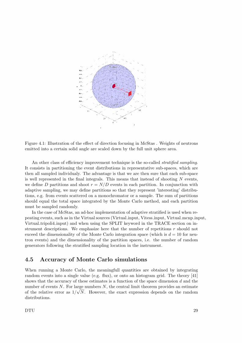
Figure 4.1: Illustration of the effect of direction focusing in McStas . Weights of neutronsemitted into a certain solid angle are scaled down by the full unit sphere area.

An other class of efficiency improvement technique is the so-called stratified sampling.It consists in partitioning the event distributions in representative sub-spaces, which arethen all sampled individualy. The advantage is that we are then sure that each sub-spaceis well represented in the final integrals. This means that instead of shooting N events,we define D partitions and shoot r = N/D events in each partition. In conjunction withadaptive sampling, we may define partitions so that they represent ’interesting’ distribu-tions, e.g. from events scattered on a monochromator or a sample. The sum of partitionsshould equal the total space integrated by the Monte Carlo method, and each partitionmust be sampled randomly.

In the case of McStas, an ad-hoc implementation of adaptive stratified is used when re-peating events, such as in the Virtual sources (Virtual input, Vitess input, Virtual mcnp input,Virtual tripoli4 input) and when using the SPLIT keyword in the TRACE section on in-strument descriptions. We emphasize here that the number of repetitions r should notexceed the dimensionality of the Monte Carlo integration space (which is d = 10 for neu-tron events) and the dimensionality of the partition spaces, i.e. the number of randomgenerators following the stratified sampling location in the instrument.

4.5 Accuracy of Monte Carlo simulations

When running a Monte Carlo, the meaningfull quantities are obtained by integratingrandom events into a single value (e.g. flux), or onto an histogram grid. The theory [41]shows that the accuracy of these estimates is a function of the space dimension d and thenumber of events N . For large numbers N , the central limit theorem provides an estimateof the relative error as 1/

√N . However, the exact expression depends on the random

distributions.

DTU 29

Records Accurarcy

103 10 %104 2.5 %105 1 %106 0.25 %107 0.05 %

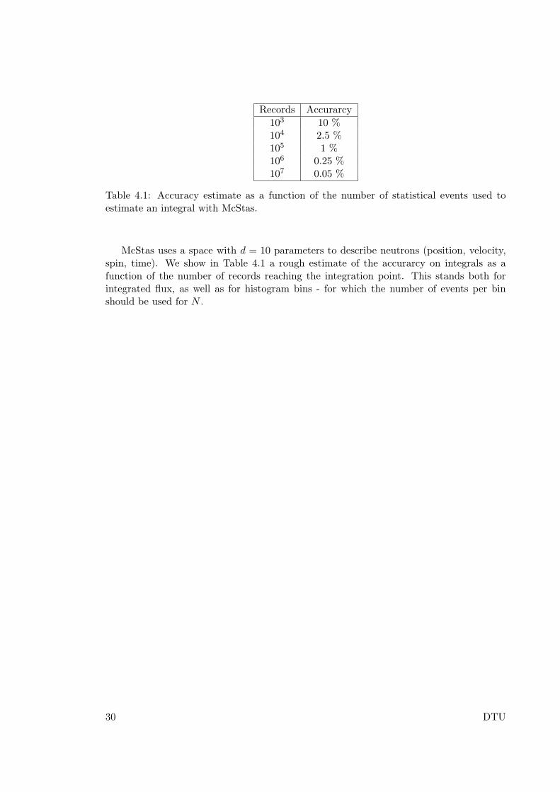
Table 4.1: Accuracy estimate as a function of the number of statistical events used toestimate an integral with McStas.

McStas uses a space with d = 10 parameters to describe neutrons (position, velocity,spin, time). We show in Table 4.1 a rough estimate of the accurarcy on integrals as afunction of the number of records reaching the integration point. This stands both forintegrated flux, as well as for histogram bins - for which the number of events per binshould be used for N .

30 DTU

Chapter 5

Running McStas

DESCRIBE NEW Python TOOLS!!

This chapter describes usage of the McStas simulation package. Refer to Chapter 3 forinstallation instructions. In case of problems regarding installation or usage, the McStasmailing list [2] or the authors should be contacted.

Important note for Windows users: It is a known problem that some of theMcStas tools do not support filenames / directories with spaces. We are working on amore general approach to this problem, which will hopefully be solved in a further release.We recommend to use ActiveState Perl 5.10. (Note that as of McStas 1.10, all neededsupport tools for Windows are bundled with McStas in a single installer file.)

Performing a simulation using McStas can be divided into the following steps/elements

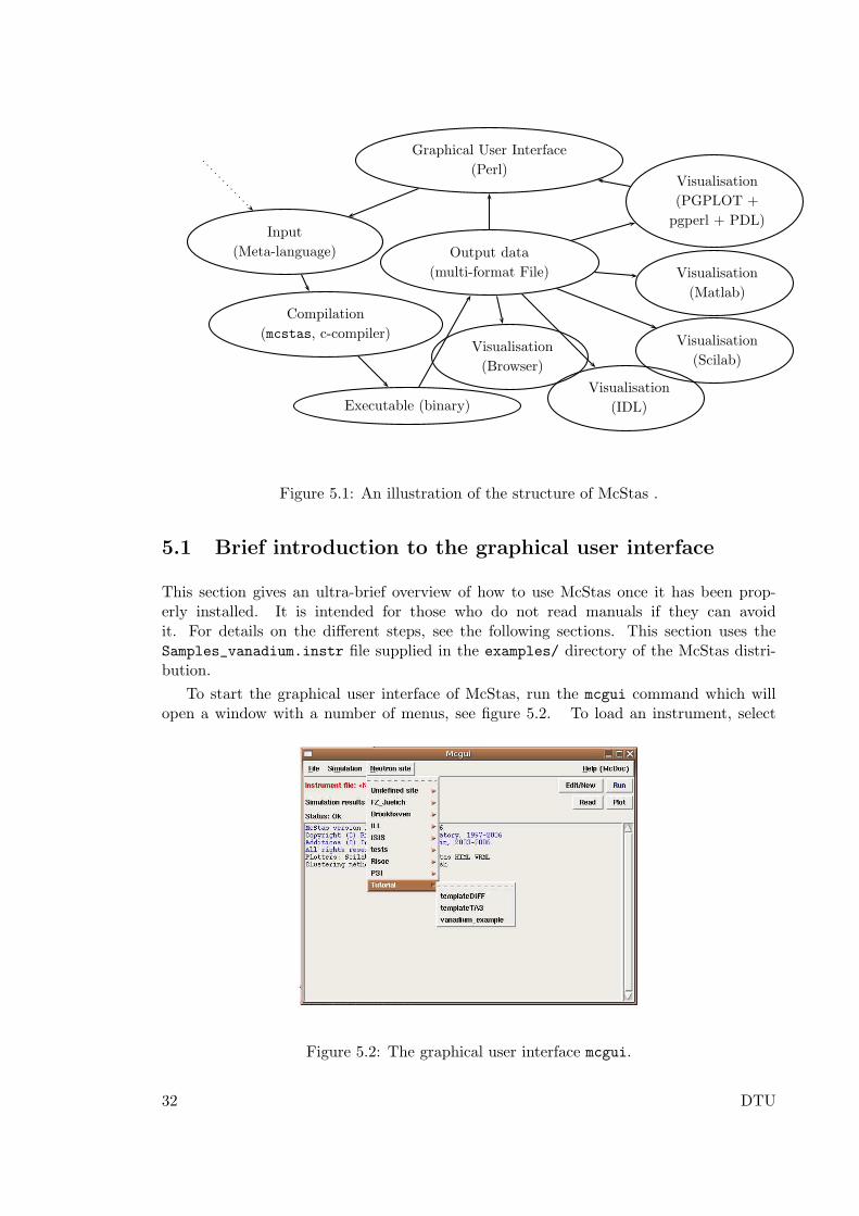
• The structure of McStas is illustrated in Figure 5.1.

• To use McStas, an instrument definition file describing the instrument to be simu-lated must be written. Alternatively, an example instrument file can be obtainedfrom the examples/ directory in the distribution or from another source.

• The input files (instrument and component files) are written in the McStas meta-language and are edited either by using your favourite editor or by using the builtin editor of the graphical user interface (mcgui).

• Next, the instrument and component files are compiled using the McStas compiler,relying on built in features from the FLEX and Bison facilities to produce a Cprogram.

• The resulting C program can then be compiled with a C compiler and run in combi-nation with various front-end programs for example to present the intensity at thedetector as a motor position is varied.

• The output data may be analyzed and visualized in the same way as regular ex-periments by using the data handling and visualisation tools in McStas based onPerl/Python in combination with chaco, matplotlib, Matlab, GNUPlot or PG-PLOT. Further data output formats including IDL, NeXus and XML are available,see section 5.5.

DTU 31

Executable (binary)

Compilation

(mcstas, c-compiler)

Output data

(multi-format File)

Input

(Meta-language)

Graphical User Interface

(Perl)Visualisation

(PGPLOT +

pgperl + PDL)

Visualisation

(Matlab)

Visualisation

(Scilab)

Visualisation

(IDL)

Visualisation

(Browser)

Figure 5.1: An illustration of the structure of McStas .

5.1 Brief introduction to the graphical user interface

This section gives an ultra-brief overview of how to use McStas once it has been prop-erly installed. It is intended for those who do not read manuals if they can avoidit. For details on the different steps, see the following sections. This section uses theSamples_vanadium.instr file supplied in the examples/ directory of the McStas distri-bution.

To start the graphical user interface of McStas, run the mcgui command which willopen a window with a number of menus, see figure 5.2. To load an instrument, select

Figure 5.2: The graphical user interface mcgui.

32 DTU

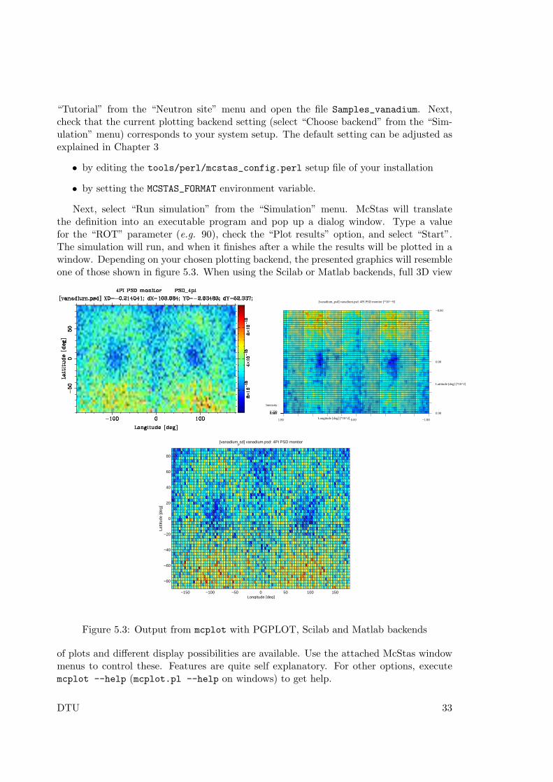
“Tutorial” from the “Neutron site” menu and open the file Samples_vanadium. Next,check that the current plotting backend setting (select “Choose backend” from the “Sim-ulation” menu) corresponds to your system setup. The default setting can be adjusted asexplained in Chapter 3

• by editing the tools/perl/mcstas_config.perl setup file of your installation

• by setting the MCSTAS_FORMAT environment variable.

Next, select “Run simulation” from the “Simulation” menu. McStas will translatethe definition into an executable program and pop up a dialog window. Type a valuefor the “ROT” parameter (e.g. 90), check the “Plot results” option, and select “Start”.The simulation will run, and when it finishes after a while the results will be plotted in awindow. Depending on your chosen plotting backend, the presented graphics will resembleone of those shown in figure 5.3. When using the Scilab or Matlab backends, full 3D view

0.5840.4070.230

Intensity

1.80 0.00 −1.80Longitude [deg] [*10^2]

0.90

0.00

−0.90

Lattitude [deg] [*10^2]

[vanadium_psd] vanadium.psd: 4PI PSD monitor [*10^−9]

−150 −100 −50 0 50 100 150

−80

−60

−40

−20

0

20

40

60

80

[vanadiumpsd] vanadium.psd: 4PI PSD monitor

Longitude [deg]

Latti

tude

[deg

]

Figure 5.3: Output from mcplot with PGPLOT, Scilab and Matlab backends

of plots and different display possibilities are available. Use the attached McStas windowmenus to control these. Features are quite self explanatory. For other options, executemcplot --help (mcplot.pl --help on windows) to get help.

DTU 33

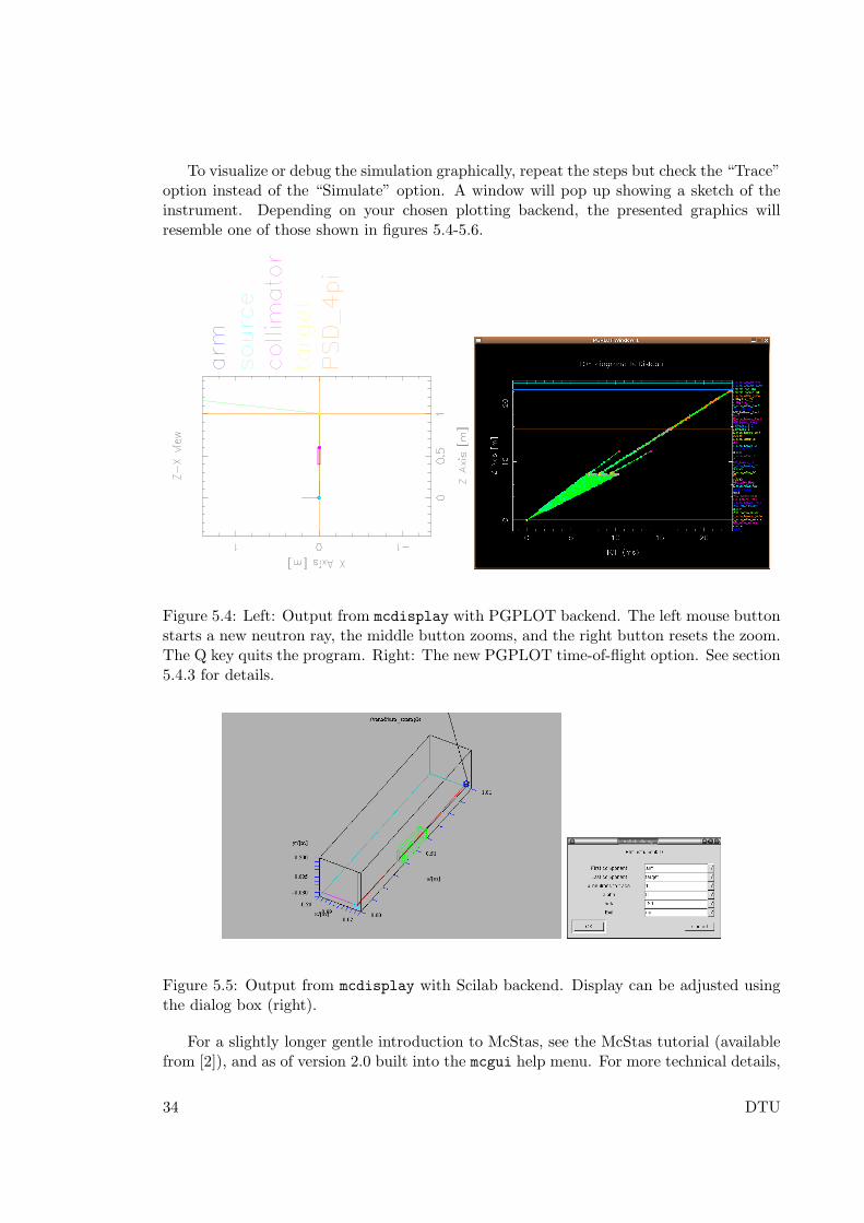
To visualize or debug the simulation graphically, repeat the steps but check the “Trace”option instead of the “Simulate” option. A window will pop up showing a sketch of theinstrument. Depending on your chosen plotting backend, the presented graphics willresemble one of those shown in figures 5.4-5.6.

Figure 5.4: Left: Output from mcdisplay with PGPLOT backend. The left mouse buttonstarts a new neutron ray, the middle button zooms, and the right button resets the zoom.The Q key quits the program. Right: The new PGPLOT time-of-flight option. See section5.4.3 for details.

Figure 5.5: Output from mcdisplay with Scilab backend. Display can be adjusted usingthe dialog box (right).

For a slightly longer gentle introduction to McStas, see the McStas tutorial (availablefrom [2]), and as of version 2.0 built into the mcgui help menu. For more technical details,

34 DTU

0

0.1

0.2

0.3

0.4

0.5

0.6

0.7

0.8

0.9

1

0

0.1

0.2

0

0.1

0.2

z/[m]

/home/fys/pkwi/Beta0/mcstas−1.7−Beta0/examples/vanadium_example

x/[m]

y/[m

]

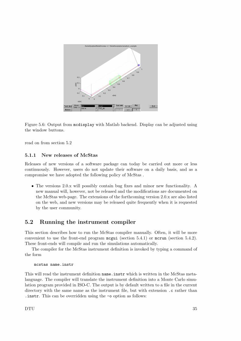
Figure 5.6: Output from mcdisplay with Matlab backend. Display can be adjusted usingthe window buttons.

read on from section 5.2

5.1.1 New releases of McStas

Releases of new versions of a software package can today be carried out more or lesscontinuously. However, users do not update their software on a daily basis, and as acompromise we have adopted the following policy of McStas .

• The versions 2.0.x will possibly contain bug fixes and minor new functionality. Anew manual will, however, not be released and the modifications are documented onthe McStas web-page. The extensions of the forthcoming version 2.0.x are also listedon the web, and new versions may be released quite frequently when it is requestedby the user community.

5.2 Running the instrument compiler

This section describes how to run the McStas compiler manually. Often, it will be moreconvenient to use the front-end program mcgui (section 5.4.1) or mcrun (section 5.4.2).These front-ends will compile and run the simulations automatically.

The compiler for the McStas instrument definition is invoked by typing a command ofthe form

mcstas name.instr

This will read the instrument definition name.instr which is written in the McStas meta-language. The compiler will translate the instrument definition into a Monte Carlo simu-lation program provided in ISO-C. The output is by default written to a file in the currentdirectory with the same name as the instrument file, but with extension .c rather than.instr. This can be overridden using the -o option as follows:

DTU 35

mcstas -o code.c name.instr

which gives the output in the file code.c. A single dash ‘-’ may be used for both inputand output filename to represent standard input and standard output, respectively.

5.2.1 Code generation options

By default, the output files from the McStas compiler are in ISO-C with some extensions(currently the only extension is the creation of new directories, which is not possible in pureISO-C). The use of extensions may be disabled with the -p or --portable option. Withthis option, the output is strictly ISO-C compliant, at the cost of some slight reduction incapabilities.

The -t or --trace option puts special “trace” code in the output. This code makes itpossible to get a complete trace of the path of every neutron ray through the instrument,as well as the position and orientation of every component. This option is mainly usedwith the mcdisplay front-end as described in section 5.4.3.

The code generation options can also be controlled by using preprocessor macros in theC compiler, without the need to re-run the McStas compiler. If the preprocessor macroMC_PORTABLE is defined, the same result is obtained as with the --portable option ofthe McStas compiler. The effect of the --trace option may be obtained by defining theMC_TRACE_ENABLED macro. Most Unix-like C compilers allow preprocessor macros to bedefined using the -D option, e.g.

cc -DMC_TRACE_ENABLED -DMC_PORTABLE ...

Finally, the --verbose option will list the components and libraries beeing included inthe instrument.

5.2.2 Specifying the location of files

The McStas compiler needs to be able to find various files during compilation, someexplicitly requested by the user (such as component definitions and files referenced by%include), and some used internally to generate the simulation executable. McStas looksfor these files in three places: first in the current directory, then in a list of directoriesgiven by the user, and finally in a special McStas directory. Usually, the user will notneed to worry about this as McStas will automatically find the required files. But if usersbuild their own component library in a separate directory or if McStas is installed in anunusual way, it will be necessary to tell the compiler where to look for the files.

The location of the special McStas directory is set when McStas is compiled. It de-faults to /usr/local/lib/mcstas on Unix-like systems and C:\mcstas\lib on Windowssystems, but it can be changed to something else, see section 3 for details. The locationcan be overridden by setting the environment variable MCSTAS:

setenv MCSTAS /home/joe/mcstas

for csh/tcsh users, or

export MCSTAS=/home/joe/mcstas

36 DTU

for bash/Bourne shell users. For Windows Users, you should define the MCSTAS from themenu ’Start/Settings/Control Panel/System/Advanced/Environment Variables’ by creat-ing MCSTAS with the value C:\mcstas\lib

To make McStas search additional directories for component definitions and includefiles, use the -I switch for the McStas compiler:

mcstas -I/home/joe/components -I/home/joe/neutron/include name.instr

Multiple -I options can be given, as shown.

5.2.3 Embedding the generated simulations in other programs

By default, McStas will generate a stand-alone C program, which is what is needed inmost cases. However, for advanced usage, such as embedding the generated simulationin another program or even including two or more simulations in the same program, astand-alone program is not appropriate. For such usage, the McStas compiler providesthe following options:

• --no-main This option makes McStas omit the main() function in the generatedsimulation program. The user must then arrange for the function mcstas_main()

to be called in some way.

• --no-runtime Normally, the generated simulation program contains all the run-timeC code necessary for declaring functions, variables, etc. used during the simulation.This option makes McStas omit the run-time code from the generated simulationprogram, and the user must then explicitly link with the file mcstas-r.c as well asother shared libraries from the McStas distribution.

Users that need these options are encouraged to contact the authors for further help.

5.2.4 Running the C compiler

After the source code for the simulation program has been generated with the McStascompiler, it must be compiled with the C compiler to produce an executable. The gener-ated C code obeys the ISO-C standard, so it should be easy to compile it using any ISO-C(or C++) compiler. E.g. a typical Unix-style command would be

cc -O -o name.out name.c -lm

The McStas team recommends these compiler alternatives for the Intel (and AMD) hard-ware architectures:

A gcc which is a very portable, open source, ISO-C compatible c compiler, availablefor most platforms. For Linux it is usually part of your distribution, for Windowsthe McStas distribution package includes a version of gcc (in the Dev-CPP sub-package), and for Mac OS X gcc is part of the Xcode tools package available on theinstallation medium.

B icc or the Intel c compiler is available for Linux, Mac OS and Windows systems andis a commercial software product. Generally, simulations run with the Intel compilerare a factor of 2 faster than the identical simulation run using gcc. To use icc

with McStas on Linux or Mac OS X, set the environment variables

DTU 37

– MCSTAS_CC=icc

– MCSTAS_CFLAGS="-g -O2 -wd177,266,1011,181"

To use icc with MPI on Unix system (see Section 5.6) installations, it seems thatediting the mpicc shell script and setting the CC variable to ”icc” is the onlyrequirement! OnWindows, the Intel c compiler is ’icl’, not ’icc’ and has a dependencyfor Microsoft Visual C++. If you have both these softwares available, runningMcStas with the Intel compiler should be possible (currently untested by the McStasdeveloper team).

The -O option typically enables the optimization phase of the compiler, which canmake quite a difference in speed of McStas generated simulations. The -o name.out setsthe name of the generated executable. The -lm options is needed on many systems to linkin the math runtime library (like the cos() and sin() functions).

Monte Carlo simulations are computationally intensive, and it is often desirable tohave them run as fast as possible. Some success can be obtained by adjusting the compileroptimization options. Here are some example platform and compiler combinations thathave been found to perform well (up-to-date information will be available on the McStasWWW home page [2]):

• Intel x86 (“PC”) with Linux and GCC, using options gcc -O3.

• Intel x86 with Linux and EGCS (GCC derivate) using options egcc -O6.

• Intel x86 with Linux and PGCC (pentium-optimized GCC derivate), using optionsgcc -O6 -mstack-align-double.

• HPPA machines running HPUX with the optional ISO-C compiler, using the op-tions -Aa +Oall -Wl,-a,archive (the -Aa option is necessary to enable the ISO-Cstandard).

• SGI machines running Irix with the options -Ofast -o32 -w

Optimization flags will typically result in a speed improvement by a factor about 3, butthe compilation of the instrument may be 5 times slower.

A warning is in place here: it is tempting to spend far more time fiddling with com-piler options and benchmarking than is actually saved in computation times. Even worse,compiler optimizations are notoriously buggy; the options given above for PGCC on Linuxand the ISO-C compiler for HPUX have been known to generate incorrect code in somecompiler versions. McStas actually puts an effort into making the task of the C com-piler easier, by in-lining code and using variables in an efficient way. As a result, McStassimulations generally run quite fast, often fast enough that further optimizations are notworthwhile. Also, optimizations are highly time and memory consuming during compila-tion, and thus may fail when dealing with large instrument descriptions (e.g. more that100 elements). The compilation process is simplified when using components of the librarymaking use of shared libraries (see SHARE keyword in chapter 6). Refer to section 5.3.4 forother optimization methods.

38 DTU

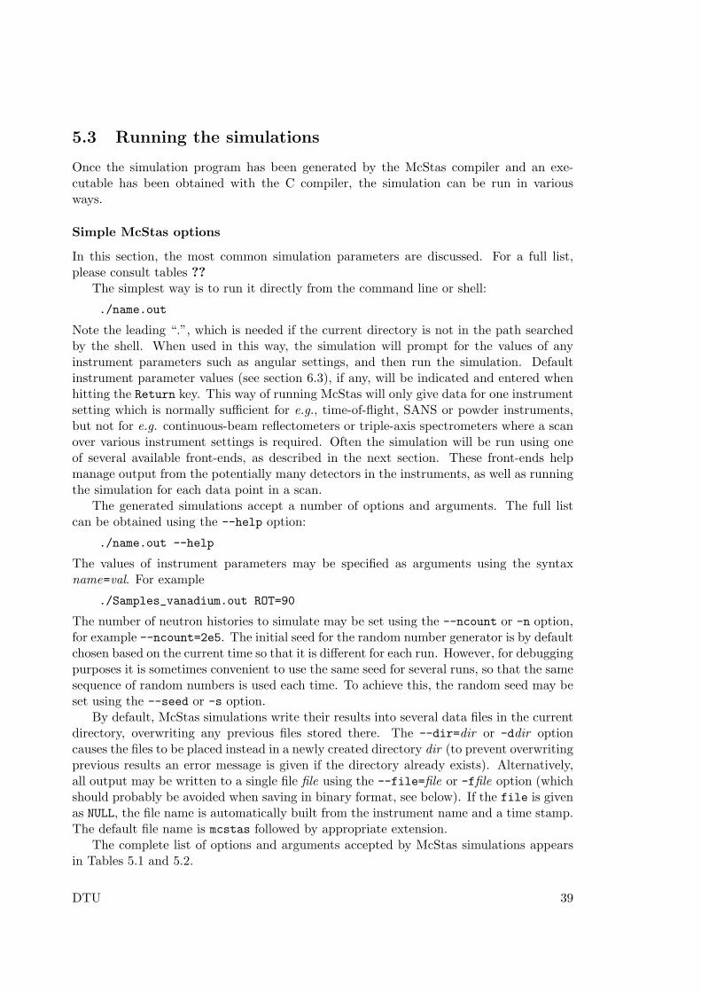
5.3 Running the simulations

Once the simulation program has been generated by the McStas compiler and an exe-cutable has been obtained with the C compiler, the simulation can be run in variousways.

Simple McStas options

In this section, the most common simulation parameters are discussed. For a full list,please consult tables ??

The simplest way is to run it directly from the command line or shell:

./name.out

Note the leading “.”, which is needed if the current directory is not in the path searchedby the shell. When used in this way, the simulation will prompt for the values of anyinstrument parameters such as angular settings, and then run the simulation. Defaultinstrument parameter values (see section 6.3), if any, will be indicated and entered whenhitting the Return key. This way of running McStas will only give data for one instrumentsetting which is normally sufficient for e.g., time-of-flight, SANS or powder instruments,but not for e.g. continuous-beam reflectometers or triple-axis spectrometers where a scanover various instrument settings is required. Often the simulation will be run using oneof several available front-ends, as described in the next section. These front-ends helpmanage output from the potentially many detectors in the instruments, as well as runningthe simulation for each data point in a scan.

The generated simulations accept a number of options and arguments. The full listcan be obtained using the --help option:

./name.out --help

The values of instrument parameters may be specified as arguments using the syntaxname=val. For example

./Samples_vanadium.out ROT=90

The number of neutron histories to simulate may be set using the --ncount or -n option,for example --ncount=2e5. The initial seed for the random number generator is by defaultchosen based on the current time so that it is different for each run. However, for debuggingpurposes it is sometimes convenient to use the same seed for several runs, so that the samesequence of random numbers is used each time. To achieve this, the random seed may beset using the --seed or -s option.

By default, McStas simulations write their results into several data files in the currentdirectory, overwriting any previous files stored there. The --dir=dir or -ddir optioncauses the files to be placed instead in a newly created directory dir (to prevent overwritingprevious results an error message is given if the directory already exists). Alternatively,all output may be written to a single file file using the --file=file or -ffile option (whichshould probably be avoided when saving in binary format, see below). If the file is givenas NULL, the file name is automatically built from the instrument name and a time stamp.The default file name is mcstas followed by appropriate extension.

The complete list of options and arguments accepted by McStas simulations appearsin Tables 5.1 and 5.2.

DTU 39

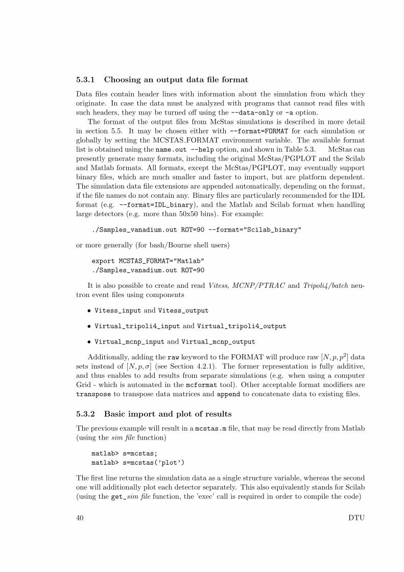
5.3.1 Choosing an output data file format

Data files contain header lines with information about the simulation from which theyoriginate. In case the data must be analyzed with programs that cannot read files withsuch headers, they may be turned off using the --data-only or -a option.

The format of the output files from McStas simulations is described in more detailin section 5.5. It may be chosen either with --format=FORMAT for each simulation orglobally by setting the MCSTAS FORMAT environment variable. The available formatlist is obtained using the name.out --help option, and shown in Table 5.3. McStas canpresently generate many formats, including the original McStas/PGPLOT and the Scilaband Matlab formats. All formats, except the McStas/PGPLOT, may eventually supportbinary files, which are much smaller and faster to import, but are platform dependent.The simulation data file extensions are appended automatically, depending on the format,if the file names do not contain any. Binary files are particularly recommended for the IDLformat (e.g. --format=IDL_binary), and the Matlab and Scilab format when handlinglarge detectors (e.g. more than 50x50 bins). For example:

./Samples_vanadium.out ROT=90 --format="Scilab_binary"

or more generally (for bash/Bourne shell users)

export MCSTAS_FORMAT="Matlab"

./Samples_vanadium.out ROT=90

It is also possible to create and read Vitess, MCNP/PTRAC and Tripoli4/batch neu-tron event files using components

• Vitess_input and Vitess_output

• Virtual_tripoli4_input and Virtual_tripoli4_output

• Virtual_mcnp_input and Virtual_mcnp_output

Additionally, adding the raw keyword to the FORMAT will produce raw [N, p, p2] datasets instead of [N, p, σ] (see Section 4.2.1). The former representation is fully additive,and thus enables to add results from separate simulations (e.g. when using a computerGrid - which is automated in the mcformat tool). Other acceptable format modifiers aretranspose to transpose data matrices and append to concatenate data to existing files.

5.3.2 Basic import and plot of results

The previous example will result in a mcstas.m file, that may be read directly from Matlab(using the sim file function)

matlab> s=mcstas;

matlab> s=mcstas(’plot’)

The first line returns the simulation data as a single structure variable, whereas the secondone will additionally plot each detector separately. This also equivalently stands for Scilab(using the get_sim file function, the ’exec’ call is required in order to compile the code)

40 DTU

-s seed--seed=seed

Set the initial seed for the random number generator. This maybe useful for testing to make each run use the same randomnumber sequence.

-n count--ncount=count

Set the number of neutron histories to simulate. The default is1,000,000. (1e6)

-d dir--dir=dir

Create a new directory dir and put all data files in that direc-tory.

-h

--help

Show a short help message with the options accepted, availableformats and the names of the parameters of the instrument.

-i

--info

Show extensive information on the simulation and the instru-ment definition it was generated from.

-t

--trace

Makes the simulation output the state of every neutron as itpasses through every component. Requires that the -t (or--trace) option is also given to the McStas compiler whenthe simulation is generated.

--no-output-files Disables the writing of data files (output to the terminal, suchas detector intensities, will still be written).

-g

--gravitation

Toggles the gravitation (approximation) handling for the wholeneutron propagation within the instrument. May producewrong results if the used components do no comply with thisoption.

--format=FORMAT Sets the file format for result simulation and data files.

-N STEPS Divide simulation into STEPS, varying parameters within givenranges ’min,max’.

param=valuemin,max

Set the value of an instrument parameter, rather than having toprompt for each one. Scans ranges are specified as ’min,max’.

Table 5.1: Options accepted by McStas simulations. For options specific to MPI andparallel computing, see section 5.6.

scilab> exec(’mcstas.sci’, -1); s=get_mcstas();

scilab> exec(’mcstas.sci’, -1); s=get_mcstas(’plot’)

and for IDL

idl> s=mcstas()

idl> s=mcstas(/plot)

See section 5.4.4 for another way of plotting simulation results using the mcplot front-end.

When choosing the HTML format, the simulation results are saved as a web page,whereas the monitor data files are saved as VRML files, displayed within the web page.

5.3.3 Interacting with a running simulation

Once the simulation has started, it is possible, under Unix, Linux and Mac OS X systems,to interact with the on-going simulation. This feature is not available when using MPI

DTU 41

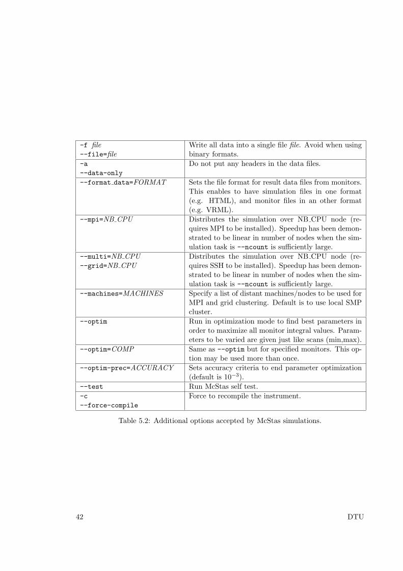
-f file--file=file

Write all data into a single file file. Avoid when usingbinary formats.

-a

--data-only

Do not put any headers in the data files.

--format data=FORMAT Sets the file format for result data files from monitors.This enables to have simulation files in one format(e.g. HTML), and monitor files in an other format(e.g. VRML).

--mpi=NB CPU Distributes the simulation over NB CPU node (re-quires MPI to be installed). Speedup has been demon-strated to be linear in number of nodes when the sim-ulation task is --ncount is sufficiently large.

--multi=NB CPU--grid=NB CPU

Distributes the simulation over NB CPU node (re-quires SSH to be installed). Speedup has been demon-strated to be linear in number of nodes when the sim-ulation task is --ncount is sufficiently large.

--machines=MACHINES Specify a list of distant machines/nodes to be used forMPI and grid clustering. Default is to use local SMPcluster.

--optim Run in optimization mode to find best parameters inorder to maximize all monitor integral values. Param-eters to be varied are given just like scans (min,max).

--optim=COMP Same as --optim but for specified monitors. This op-tion may be used more than once.

--optim-prec=ACCURACY Sets accuracy criteria to end parameter optimization(default is 10−3).

--test Run McStas self test.

-c

--force-compile

Force to recompile the instrument.

Table 5.2: Additional options accepted by McStas simulations.

42 DTU

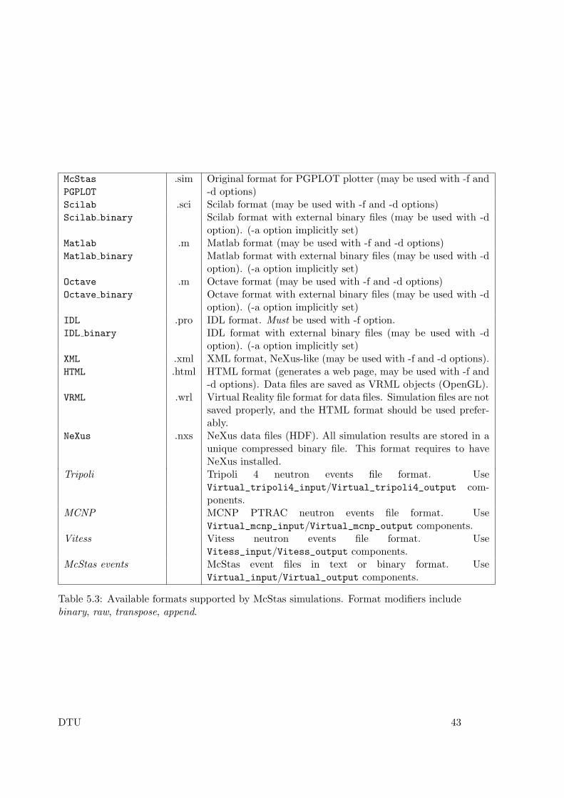
McStas

PGPLOT

.sim Original format for PGPLOT plotter (may be used with -f and-d options)

Scilab .sci Scilab format (may be used with -f and -d options)Scilab binary Scilab format with external binary files (may be used with -d

option). (-a option implicitly set)Matlab .m Matlab format (may be used with -f and -d options)Matlab binary Matlab format with external binary files (may be used with -d

option). (-a option implicitly set)Octave .m Octave format (may be used with -f and -d options)Octave binary Octave format with external binary files (may be used with -d

option). (-a option implicitly set)IDL .pro IDL format. Must be used with -f option.IDL binary IDL format with external binary files (may be used with -d

option). (-a option implicitly set)XML .xml XML format, NeXus-like (may be used with -f and -d options).HTML .html HTML format (generates a web page, may be used with -f and

-d options). Data files are saved as VRML objects (OpenGL).VRML .wrl Virtual Reality file format for data files. Simulation files are not

saved properly, and the HTML format should be used prefer-ably.

NeXus .nxs NeXus data files (HDF). All simulation results are stored in aunique compressed binary file. This format requires to haveNeXus installed.

Tripoli Tripoli 4 neutron events file format. UseVirtual_tripoli4_input/Virtual_tripoli4_output com-ponents.

MCNP MCNP PTRAC neutron events file format. UseVirtual_mcnp_input/Virtual_mcnp_output components.

Vitess Vitess neutron events file format. UseVitess_input/Vitess_output components.

McStas events McStas event files in text or binary format. UseVirtual_input/Virtual_output components.

Table 5.3: Available formats supported by McStas simulations. Format modifiers includebinary, raw, transpose, append.

DTU 43

parallelization.McStas attaches a signal handler to the simulation process. In order to send a signal to

the process, the process-id pid must be known. Users may look at their running processeswith the Unix ’ps’ command, or alternatively process managers like ’top’ and ’gtop’. If afile.out simulation obtained from McStas is running, the process status command shouldoutput a line resembling

<user> 13277 7140 99 23:52 pts/2 00:00:13 file.out

where user is your Unix login. The pid is there ’13277’.Once known, it is possible to send one of the signals listed in Table 5.4 using the ’kill’

unix command (or the functionalities of your process manager), e.g.

kill -USR2 13277

This will result in a message showing status (here 33 % achieved), as well as the positionin the instrument of the current neutron.

# McStas: [pid 13277] Signal 12 detected SIGUSR2 (Save simulation)

# Simulation: file (file.instr)

# Breakpoint: MyDetector (Trace) 33.37 % ( 333654.0/ 1000000.0)

# Date : Wed May 7 00:00:52 2003

# McStas: Saving data and resume simulation (continue)

followed by the list of detector outputs (integrated counts and files). Finally, sending akill 13277 (which is equivalent to kill -TERM 13277) will end the simulation before theinitial ’ncount’ preset.

A typical usage example would be, for instance, to save data during a simulation, plotor analyze it, and decide to interrupt the simulation earlier if the desired statistics hasbeen achieved. This may be done automatically using the Progress_bar component.

Whenever simulation data is generated before end (or the simulation is interrupted),the ’ratio’ field of the monitored data will provide the level of achievement of the computa-tion (for instance ’3.33e+05/1e+06’). Intensities are then usually to be scaled accordinglyby the user.

Additionally, any system error will result in similar messages, giving indication aboutthe occurrence of the error (component and section). Whenever possible, the simulationwill try to save the data before ending. Most errors appear when using a newly writtencomponent, in the INITIALIZE, TRACE or FINALLY sections. Memory errors usually showup when C pointers have not been allocated/unallocated before usage, whereas mathe-matical errors are found when, for instance, dividing by zero.

5.3.4 Optimizing simulation speed

There are various ways to speed up simulations

• Optimize the compilation of the instrument, as explained in section 5.2.4.

• Execute the simulation in parallel on a computer grid or a cluster (with MPI or sshgrid ) as explained in section 5.6.

44 DTU

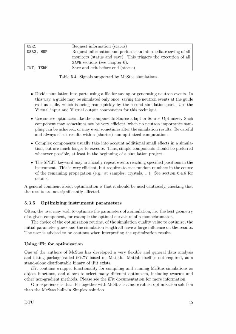
USR1 Request information (status)USR2, HUP Request information and performs an intermediate saving of all

monitors (status and save). This triggers the execution of allSAVE sections (see chapter 6).

INT, TERM Save and exit before end (status)

Table 5.4: Signals supported by McStas simulations.

• Divide simulation into parts using a file for saving or generating neutron events. Inthis way, a guide may be simulated only once, saving the neutron events at the guideexit as a file, which is being read quickly by the second simulation part. Use theVirtual input and Virtual output components for this technique.

• Use source optimizers like the components Source adapt or Source Optimizer. Suchcomponent may sometimes not be very efficient, when no neutron importance sam-pling can be achieved, or may even sometimes alter the simulation results. Be carefuland always check results with a (shorter) non-optimized computation.

• Complex components usually take into account additional small effects in a simula-tion, but are much longer to execute. Thus, simple components should be preferredwhenever possible, at least in the beginning of a simulation project.

• The SPLIT keyword may artificially repeat events reaching specified positions in theinstrument. This is very efficient, but requires to cast random numbers in the courseof the remaining propagation (e.g. at samples, crystals, ...). See section 6.4.6 fordetails.

A general comment about optimization is that it should be used cautiously, checking thatthe results are not significantly affected.

5.3.5 Optimizing instrument parameters

Often, the user may wish to optimize the parameters of a simulation, i.e. the best geometryof a given component, for example the optimal curvature of a monochromator.

The choice of the optimization routine, of the simulation quality value to optimize, theinitial parameter guess and the simulation length all have a large influence on the results.The user is advised to be cautious when interpreting the optimization results.

Using iFit for optimization

One of the authors of McStas has developed a very flexible and general data analysisand fitting package called iFit?? based on Matlab. Matlab itself is not required, as astand-alone distributable binary of iFit exists.

iFit contains wrapper functionality for compiling and running McStas simulations asobject functions, and allows to select many different optimizers, including swarms andother non-gradient methods. Please see the iFit documentation for more information.

Our experience is that iFit together with McStas is a more robust optimization solutionthan the McStas built-in Simplex solution.

DTU 45

Using the Simplex method

The McStas package comes with a Simplex optimization method to find best instrumentparameters in order to maximize all or some specified monitor integrated values. It usesthe Downhill Simplex Method in Multidimensions [45, 46] which is a geometric optimiza-tion method somewhat similar to genetic algorithms. It is not as fast as the gradientmethod, but is much more robust. It is well suited for problems with up to about 10-20 parameters to optimize. Higher dimensionalities are not guarantied to converge to ameaningful solution.

When using mcrun (section 5.4.2), the optimization mode is set by using the --optimoption or a list of monitors to maximize with as many --optim=COMP as required. Theoptimization accuracy criterion may be changed with the --optim-prec=accuracy option.

From mcgui (section 5.4.1), one should choose the ’Optimization’ execution mode(instead of the Simulation or Trace mode). Then specify the instrument parameters tooptimize by indicating their variation range param=min,max (e.g. Lambda=1,4) just likeparameter scans. Optionally, the starting guess value might be given with the syntaxparam=min,guess,max. The optimization accuracy criterion is controlled using the ’Pre-cision’ entry box in the configuration options (See Figure 5.7). Finally, run the simulation.The optimum set of parameters is then printed at the end of the simulation process. Youmay ask to maximize only given monitors (instead of all) by selecting their componentnames in the lower lists in the Run Dialog (up to 3).

If you would like to maximize the flux at a given monitor, with some divergenceconstrains, you should for instance simply add a divergence collimator before the monitor.Alternatively, write a new component that produce the required ’figure-of-merit’.

The optimization search interval constrains the evolution of parameters. It should bechosen carefully. In particular it is safer for it to indeed contain a high signal domain, andbe preferably symmetric with respect to that maximum.

Using custom optimization routines

The user should write a function script or a program that

• inputs the simulation parameters, which are usually numerical values such as TT inthe prisma2 instrument from the examples directory of the package.

• builds a command line from these parameters.

• executes that command, and waits until the end of the computation.

• reads the relevant data from the monitors.

• outputs a simulation quality measurement from this data, usually the integratedcounts or some peak width.

For instance, for the prisma2 instrument we could write a function for Matlab (seesection 5.5 for details about the Matlab data format) in order to study the effects of theTT parameter:

46 DTU

function y = instr_value(p)

TT = p(1); % p may be a vector/matrix containing many parameters

syscmd = [ ’mcrun prisma2.instr -n1e5 TT=’ num2str(TT) ...

’ PHA=22 PHA1=-3 PHA2=-2 PHA3=-1 PHA4=0 PHA5=1’ ...

’ PHA6=2 PHA7=3 TTA=44 --format="Matlab binary"’ ];

system(syscmd); path(path) % execute simulation, and rehash files

s = mcstas; % get the simulation data, and the monitor data

s = s.prisma2.m_mcstas.detector.prisma2_tof.signal;

eval(s); % we could also use the ’statistics’ field

y = -Mean; % ’value’ of the simulation

Then a numerical optimization should be available, such as those provided with Matlab,Scilab, IDL, and Perl-PDL high level languages. In this example, we may wish to maximizethe instr_value function value. The fminsearch function of Matlab is a minimizationmethod (that’s why we have a minus sign for y value), and:

matlab> TT = fminsearch(’instr_value’, -25)

will determine the best value of TT, starting from -25 estimate, in order to minimizefunction instr_value, and thus maximize the mean detector counts.

5.4 Using simulation front-ends

McStas includes a number of front-end programs that extend the functionality of thesimulations. A front-end program is an interface between the user and the simulations,running the simulations and presenting the output in various ways to the user.

The list of available McStas front-end programs may be obtained from the mcdoc --tools

command:

McStas Tools

mcstas Main instrument compiler

mcrun Instrument build and execution utility

mcgui Graphical User Interface instrument builder

mcdoc Component library documentation generator/viewer

mcplot Simulation result viewer

mcdisplay Instrument geometry viewer

mcresplot Instrument resolution function viewer

mcstas2vitess McStas to Vitess component translation utility

mcconvert Matlab <-> Scilab script conversion tool

mcformat Conversion tool for text files and MPI/grids

mcformatgui GUI for mcformat

mcdaemon Instrument results on-line plotting

When used with the -h flag, all tools display a specific help.

SEE ALSO: mcstas, mcdoc, mcplot, mcrun, mcgui, mcresplot, mcstas2vitess

DOC: Please visit http://www.mcstas.org

DTU 47

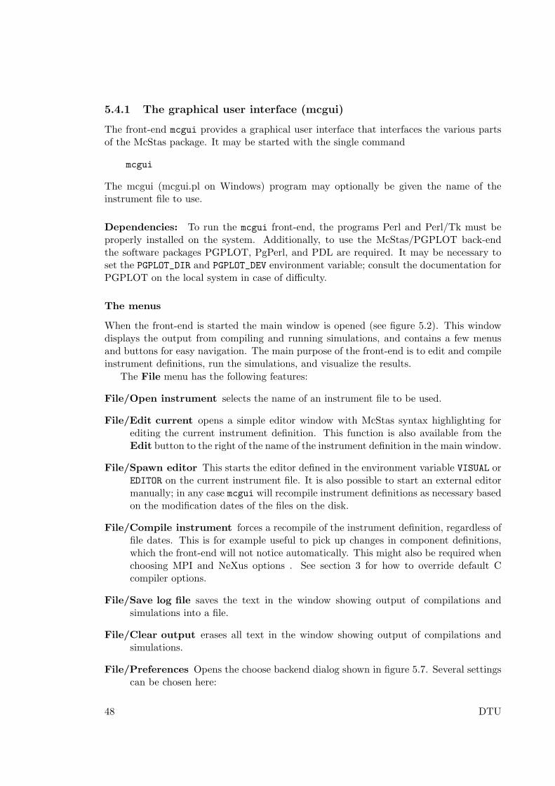
5.4.1 The graphical user interface (mcgui)

The front-end mcgui provides a graphical user interface that interfaces the various partsof the McStas package. It may be started with the single command

mcgui

The mcgui (mcgui.pl on Windows) program may optionally be given the name of theinstrument file to use.

Dependencies: To run the mcgui front-end, the programs Perl and Perl/Tk must beproperly installed on the system. Additionally, to use the McStas/PGPLOT back-endthe software packages PGPLOT, PgPerl, and PDL are required. It may be necessary toset the PGPLOT_DIR and PGPLOT_DEV environment variable; consult the documentation forPGPLOT on the local system in case of difficulty.

The menus

When the front-end is started the main window is opened (see figure 5.2). This windowdisplays the output from compiling and running simulations, and contains a few menusand buttons for easy navigation. The main purpose of the front-end is to edit and compileinstrument definitions, run the simulations, and visualize the results.

The File menu has the following features:

File/Open instrument selects the name of an instrument file to be used.

File/Edit current opens a simple editor window with McStas syntax highlighting forediting the current instrument definition. This function is also available from theEdit button to the right of the name of the instrument definition in the main window.

File/Spawn editor This starts the editor defined in the environment variable VISUAL orEDITOR on the current instrument file. It is also possible to start an external editormanually; in any case mcgui will recompile instrument definitions as necessary basedon the modification dates of the files on the disk.

File/Compile instrument forces a recompile of the instrument definition, regardless offile dates. This is for example useful to pick up changes in component definitions,which the front-end will not notice automatically. This might also be required whenchoosing MPI and NeXus options . See section 3 for how to override default Ccompiler options.

File/Save log file saves the text in the window showing output of compilations andsimulations into a file.

File/Clear output erases all text in the window showing output of compilations andsimulations.

File/Preferences Opens the choose backend dialog shown in figure 5.7. Several settingscan be chosen here:

48 DTU

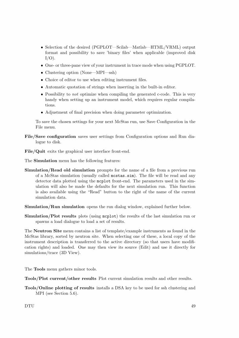
• Selection of the desired (PGPLOT—Scilab—Matlab—HTML/VRML) outputformat and possibility to save ’binary files’ when applicable (improved diskI/O).

• One- or three-pane view of your instrument in trace mode when using PGPLOT.

• Clustering option (None—MPI—ssh)

• Choice of editor to use when editing instrument files.

• Automatic quotation of strings when inserting in the built-in editor.

• Possibility to not optimize when compiling the generated c-code. This is veryhandy when setting up an instrument model, which requires regular compila-tions.

• Adjustment of final precision when doing parameter optimization.

To save the chosen settings for your next McStas run, use Save Configuration in theFile menu.

File/Save configuration saves user settings from Configuration options and Run dia-logue to disk.

File/Quit exits the graphical user interface front-end.

The Simulation menu has the following features:

Simulation/Read old simulation prompts for the name of a file from a previous runof a McStas simulation (usually called mcstas.sim). The file will be read and anydetector data plotted using the mcplot front-end. The parameters used in the sim-ulation will also be made the defaults for the next simulation run. This functionis also available using the “Read” button to the right of the name of the currentsimulation data.

Simulation/Run simulation opens the run dialog window, explained further below.

Simulation/Plot results plots (using mcplot) the results of the last simulation run orspawns a load dialogue to load a set of results.

The Neutron Site menu contains a list of template/example instruments as found in theMcStas library, sorted by neutron site. When selecting one of these, a local copy of theinstrument description is transferred to the active directory (so that users have modifi-cation rights) and loaded. One may then view its source (Edit) and use it directly forsimulations/trace (3D View).

The Tools menu gathers minor tools.

Tools/Plot current/other results Plot current simulation results and other results.

Tools/Online plotting of results installs a DSA key to be used for ssh clustering andMPI (see Section 5.6).

DTU 49

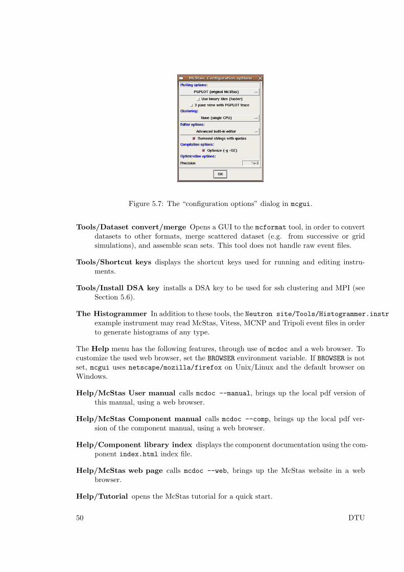
Figure 5.7: The “configuration options” dialog in mcgui.

Tools/Dataset convert/merge Opens a GUI to the mcformat tool, in order to convertdatasets to other formats, merge scattered dataset (e.g. from successive or gridsimulations), and assemble scan sets. This tool does not handle raw event files.

Tools/Shortcut keys displays the shortcut keys used for running and editing instru-ments.

Tools/Install DSA key installs a DSA key to be used for ssh clustering and MPI (seeSection 5.6).

The Histogrammer In addition to these tools, the Neutron site/Tools/Histogrammer.instr

example instrument may read McStas, Vitess, MCNP and Tripoli event files in orderto generate histograms of any type.

The Help menu has the following features, through use of mcdoc and a web browser. Tocustomize the used web browser, set the BROWSER environment variable. If BROWSER is notset, mcgui uses netscape/mozilla/firefox on Unix/Linux and the default browser onWindows.

Help/McStas User manual calls mcdoc --manual, brings up the local pdf version ofthis manual, using a web browser.

Help/McStas Component manual calls mcdoc --comp, brings up the local pdf ver-sion of the component manual, using a web browser.

Help/Component library index displays the component documentation using the com-ponent index.html index file.

Help/McStas web page calls mcdoc --web, brings up the McStas website in a webbrowser.

Help/Tutorial opens the McStas tutorial for a quick start.

50 DTU

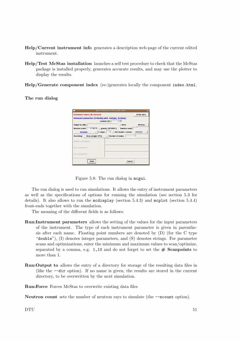
Help/Current instrument info generates a description web-page of the current editedinstrument.

Help/Test McStas installation launches a self test procedure to check that the McStaspackage is installed properly, generates accurate results, and may use the plotter todisplay the results.

Help/Generate component index (re-)generates locally the component index.html.

The run dialog

Figure 5.8: The run dialog in mcgui.

The run dialog is used to run simulations. It allows the entry of instrument parametersas well as the specifications of options for running the simulation (see section 5.3 fordetails). It also allows to run the mcdisplay (section 5.4.3) and mcplot (section 5.4.4)front-ends together with the simulation.

The meaning of the different fields is as follows:

Run:Instrument parameters allows the setting of the values for the input parametersof the instrument. The type of each instrument parameter is given in parenthe-sis after each name. Floating point numbers are denoted by (D) (for the C type“double”), (I) denotes integer parameters, and (S) denotes strings. For parameterscans and optimizations, enter the minimum and maximum values to scan/optimize,separated by a comma, e.g. 1,10 and do not forget to set the # Scanpoints tomore than 1.

Run:Output to allows the entry of a directory for storage of the resulting data files in(like the --dir option). If no name is given, the results are stored in the currentdirectory, to be overwritten by the next simulation.

Run:Force Forces McStas to overwrite existing data files

Neutron count sets the number of neutron rays to simulate (the --ncount option).

DTU 51

Run:Gravity Activates gravitation handling. Not all components full support the useof gravitation, but all transport in “free space” using the PROP DT, PROP Z0etc. macros will include propagation with gravity. Only local, internal componentpropagation without the PROP routines will be gravity-less. As a conclusion itis considered safe and to high precision correct to apply the gravitation setting ifone takes care to use the Guide gravity component and other gravity-supportingguide types in combination with non-gravity components that are “small” in size,i.e. samples, lenses, etc.

Run:Random seed/Set seed to selects between using a random seed (different in eachsimulation) for the random number generator, or using a fixed seed (to reproduceresults for debugging).

Run:Simulate/Trace (3D)/Optimize selects between several modes of running thesimulation:

• Simulate: perform a normal simulation or a scan when #steps is set to non-zerovalue

• Trace (3D view): View the instrument in 3D tracing individual neutrons throughthe instrument

• Optimize: find the optimum value of the simulation parameters in the givenranges (see section 5.3.5).

• Backgrounding (bg): Simulate or Optimize in the background.

Run:# steps / # optim sets the number of simulation to run when performing a pa-rameter scan or the number of iterations to perform in optimization mode.

Run:Plot results – if checked, the mcplot front-end will be run after the simulation hasfinished, and the plot dialog will appear (see below).

Run:Format quick selection of output format. Binary mode may be checked from the“Simulation/Configuration options” dialog box.

Run:Clustering method selects the mechanism to be used for running on grids andclusters. See section 5.6 on parallel computing for more informations.

Run:Number of nodes sets the number of nodes to use for MPI/ssh clustering.

Run:Inspect component (Trace mode) will trace only neutron trajectories that reacha given component (e.g. sample or detector).

Run:First component (Trace mode) seletcs the first component to plot (default is first)in order to define a region of interest.

Run:Last component (Trace mode) seletcs the last component to plot (default is first)in order to define a region of interest.

Run:Maximize monitor (Optimization mode) seletcs up to three monitors which inte-gral value should be maximized, varying instrument parameters. If no monitor isselected, the sum of all monitors is optimized.

52 DTU

Run:Start runs the simulation.

Run:Cancel aborts the dialog.

Most of the settings on the run dialog can be saved for your next McStas run using ’Saveconfiguration’ in the File menu.

Before running the simulation, the instrument definition is automatically compiledif it is newer than the generated C file (or if the C file is newer than the executable).The executable is assumed to have a .out suffix in the filename. NB: If components arechanged, automatic compilation is not performed. Instead, use the File/Compile menuitem in mcgui.

The editor window

The editor window provides a simple editor for creating and modifying instrument defini-tions. Apart from the usual editor functions, the “Insert” menu provides some functionsthat aid in the construction of the instrument definitions:

Editor Insert/Instrument template inserts the text for a simple instrument skeletonin the editor window.

Editor Insert/Component. . . opens up a dialog window with a list of all the compo-nents available for use in McStas. Selecting a component will display a description.Double-clicking will open up a dialog window allowing the entry of the values ofall the parameters for the component (figure 5.9). See section 6.3 for details of themeaning of the different fields.

The dialog will also pick up those of the users own components that are presentin the current directory when mcgui is started. See section 6.7 for how to writecomponents to integrate well with this facility.

Editor Insert/Type These menu entries give quick access to the entry dialog for thevarious component types available, i.e. Sources, Optics, Samples, Monitors, Misc,Contrib and Obsolete.

5.4.2 Running simulations on the commandline (mcrun)

The mcrun front-end (mcrun.pl on Windows) provides a convenient command-line interfacefor running simulations with the same automatic compilation features available in themcgui front-end. It also provides a facility for running a series of simulations while varyingan input parameter.

The command

mcrun sim args ...

will compile the instrument definition sim.instr (if necessary) into an executable simu-lation sim.out. It will then run sim.out, passing the argument list args

The possible arguments are the same as those accepted by the simulations themselvesas described in section 5.3, with the following extensions:

DTU 53

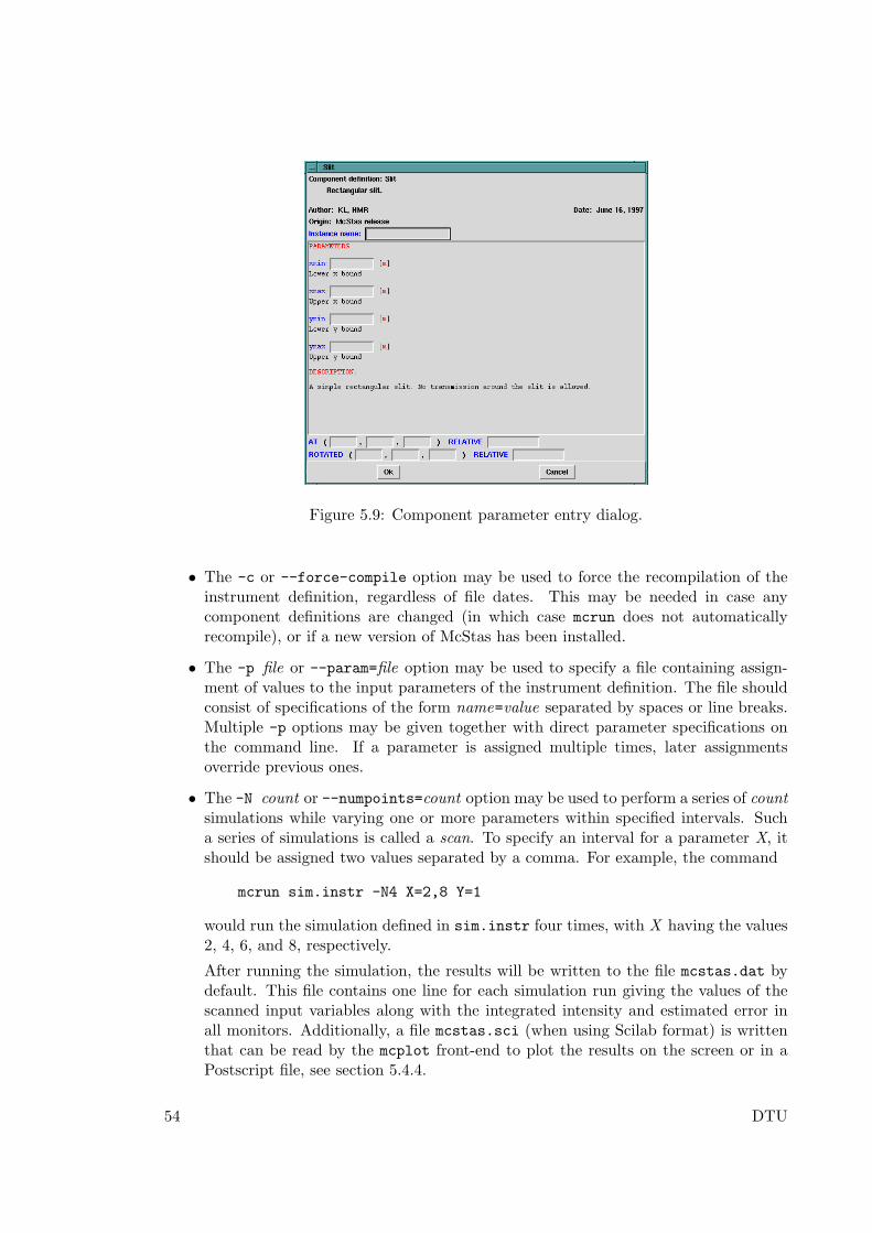
Figure 5.9: Component parameter entry dialog.

• The -c or --force-compile option may be used to force the recompilation of theinstrument definition, regardless of file dates. This may be needed in case anycomponent definitions are changed (in which case mcrun does not automaticallyrecompile), or if a new version of McStas has been installed.

• The -p file or --param=file option may be used to specify a file containing assign-ment of values to the input parameters of the instrument definition. The file shouldconsist of specifications of the form name=value separated by spaces or line breaks.Multiple -p options may be given together with direct parameter specifications onthe command line. If a parameter is assigned multiple times, later assignmentsoverride previous ones.

• The -N count or --numpoints=count option may be used to perform a series of countsimulations while varying one or more parameters within specified intervals. Sucha series of simulations is called a scan. To specify an interval for a parameter X, itshould be assigned two values separated by a comma. For example, the command

mcrun sim.instr -N4 X=2,8 Y=1

would run the simulation defined in sim.instr four times, with X having the values2, 4, 6, and 8, respectively.

After running the simulation, the results will be written to the file mcstas.dat bydefault. This file contains one line for each simulation run giving the values of thescanned input variables along with the integrated intensity and estimated error inall monitors. Additionally, a file mcstas.sci (when using Scilab format) is writtenthat can be read by the mcplot front-end to plot the results on the screen or in aPostscript file, see section 5.4.4.

54 DTU

• When performing a scan, the -f file and --file=file options make mcrun write theoutput to the files file.dat and file.sim instead of the default names.

• When performing a scan, the -d dir and --dir=dir options make mcrun put alloutput in a newly created directory dir. Additionally, the directory will have sub-directories 1, 2, 3,. . . containing all data files output from the different simulations.When the -d option is not used, no data files are written from the individual simu-lations (in order to save disk space).

• The mcrun --test command will test your McStas installation, accuracy and plot-ter.

The -h option will list valid options. The mcrun front-end requires a working installa-tion of Perl to run.

5.4.3 Graphical display of simulations (mcdisplay)

The front-end mcdisplay (mcdisplay.pl on Windows) is a graphical visualization tool,very useful for debugging. It presents a schematic drawing of the instrument definition,showing the position of the components and the paths of the simulated neutrons throughthe instrument. It is thus very useful for debugging a simulation, for example to spotcomponents in the wrong position or to find out where neutrons are getting lost. (Seefigures 5.4-5.6.)

To use the mcdisplay front-end with a simulation, run it as follows:

mcdisplay sim args . . .

where sim is the name of either the instrument source sim.instr or the simulation pro-gram sim.out generated with McStas, and args . . . are the normal command line argu-ments for the simulation, as explained above. The -h option will list valid options.

The drawing back-end program may be selected among PGPLOT, VRML, Matlaband Scilab using either the -pPLOTTER option or using the current MCSTAS_FORMAT

environment variable. For instance, calling

mcdisplay -pScilab ./Samples_vanadium.out ROT=90

or (csh/tcsh syntax)

setenv MCSTAS_FORMAT Scilab

mcdisplay ./Samples_vanadium.out ROT=90

will output graphics using Scilab. The mcdisplay front-end can also be run from the mcguifront-end. Examples of plotter appearence for mcdisplay is shown in figures 5.4-5.6.

McStas/PGPLOT back-end This will view the instrument from above. A multi-display that shows the instrument from three directions simultaneously can be shownusing the --multi option:

mcdisplay --multi sim.out args . . .

DTU 55

Click the left mouse button in the graphics window or hit the space key to see thedisplay of successive neutron trajectories. The ‘P’ key saves a postscript file containingthe current display that can be sent to the printer to obtain a hardcopy; the ‘C’ keyproduces color postscript. To stop the simulation prematurely, type ‘Q’ or use control-Cas normal in the window in which mcdisplay was started.

To see details in the instrument, it is possible to zoom in on a part of the instrumentusing the middle mouse button (or the ‘Z’ key on systems with a one- or two-buttonmouse). The right mouse button (or the ‘X’ key) resets the zoom. Note that afterzooming, the aspect ratio of the plot may have changed, and thus the angles as seen onthe display may not match the actual angles.

Another way to see details while maintaining an overview of the instrument is to use the--zoom=factor option. This magnifies the display of each component along the selectedaxis only, e.g. a Soller collimator is magnified perpendicular to the neutron beam butnot along it. This option may produce rather strange visual effects as the neutron passesbetween components with different coordinate magnifications, but it is occasionally useful.

When debugging, it is often the case that one is interested only in neutrons that reacha particular component in the instrument. For example, if there is a problem with thesample one may prefer not to see the neutrons that are absorbed in the monochromatorshielding. For these cases, the --inspect=comp option is useful. With this option, onlyneutrons that reach the component named comp are shown in the graphics display.

As of McStas 1.10, the PGPLOT version has a special mode for time of flight ap-plications. Using the new commandline options --TOF/-T and --tmax=TMAX, chopperacceptance diagrams can be generated from the statistical information from the simulatedneutron rays. As the use in non-interactive, please use with a limited number of neutronrays (-n/--ncount). For export of graphics, combine with e.g. --gif.

The mcdisplay front-end will then require the Perl, the PGPLOT, and the PGPerlpackages to be installed. It may be necessary to set the PGPLOT_DIR and PGPLOT_DEV

environment variable; consult the documentation for PGPLOT on the local system incase of difficulty.

Matlab and Scilab back-ends A 3D view of the instrument, and various operations(zoom, export, print, trace neutrons, . . . ) is available from dedicated Graphical UserInterfaces. The --inspect option may be used (see previous paragraph), as well as the--first and --last options to specify a region of interest. Note: The Scilab plotter forWindows does not allow to rotate interactively the 3D view, and you are to use the alphaand theta choices in the pop-up Dialog.

The mcdisplay front-end will then require the Perl, and either Scilab or Matlab to beinstalled.

VRML/OpenGL back-ends When using the -pVRML option, the instrument is shownin Virtual Reality (using OpenGL). You may then walk aside instrument, or go insideelements following neutron trajectories. As all neutron trajectories are stored into a VRMLfile, you better limit the number of stored trajectories below 1000, otherwise file size andprocessing time becomes significant. The --inspect option is not available in VRMLformat display.

56 DTU

5.4.4 Plotting the results of a simulation (mcplot)

The front-end mcplot (mcplot.pl on Windows) is a program that produces plots of all themonitors in a simulation, and it is thus useful to get a quick overview of the simulationresults.

In the simplest case, the front-end is run simply by typing

mcplot

This will plot any simulation data stored in the current directory, which is where simula-tions store their results by default. If the --dir or --file options have been used (seesection 5.3), the name of the file or directory should be passed to mcplot, e.g. “mcplotdir” or “mcplot file”. It is also possible to plot one single text (not binary) data file froma given monitor, passing its name to mcplot.

The drawing back-end program may be selected among PGPLOT, VRML, Matlab andScilab using either the -pPLOTTER option (e.g. mcplot -pScilab file) or using thecurrent MCSTAS_FORMAT environment variable. Moreover, the drawing back-end programwill also be set depending on the file extension (see Table 5.3).

It should be emphasised that mcplot may only display simulation results with theformat that was chosen during the computation. Indeed, if you request data in a givenformat from a simulation, you will only be able to display results using that same drawingback-end.

Anyway, the mcconvert utility may convert a McStas data file between Matlab andScilab formats (see section 5.4.8), also handling binary data sets. Alternatively, themcformat utility will convert any McStas result into data format (see section 5.4.9), butrestricting to text data sets. In this case, we recommend to generate data sets usingPGPLOT/McStas format, and translate into any other format using mcformat.

The mcplot front-end can also be run from the mcgui front-end.

The initial display shows plots for each detector in the simulation. Examples of plotterappearence for mcplot is shown in figures 5.4-5.3.

McStas/PGPLOT back-end Clicking the left mouse button on a plot produces a full-window version of that plot. The ‘P’ key saves a postscript file containing the current plotthat can be sent to the printer to obtain a hardcopy; the ‘C’ key produces color postscript.The ‘Q’ key quits the program (or CTRL-C in the controlling terminal may be used asnormal).

To use the mcplot front-end with PGPLOT, the programs Perl, PGPLOT, PgPerl,and PDL must all be properly installed on the system. It may be necessary to set thePGPLOT_DIR and PGPLOT_DEV environment variable; consult the documentation for PG-PLOT on the local system in case of difficulty.

Matlab and Scilab back-ends A dedicated McStas/Mcplot Dialog or menu attachedto the plotting window is available, and provides many operations (duplication, export,colormaps, . . . ). The corresponding ’mcplot’ Matlab and Scilab functions may be calledfrom these language prompt with the same method as in section 5.3, e.g:

matlab> s=mcplot;

DTU 57

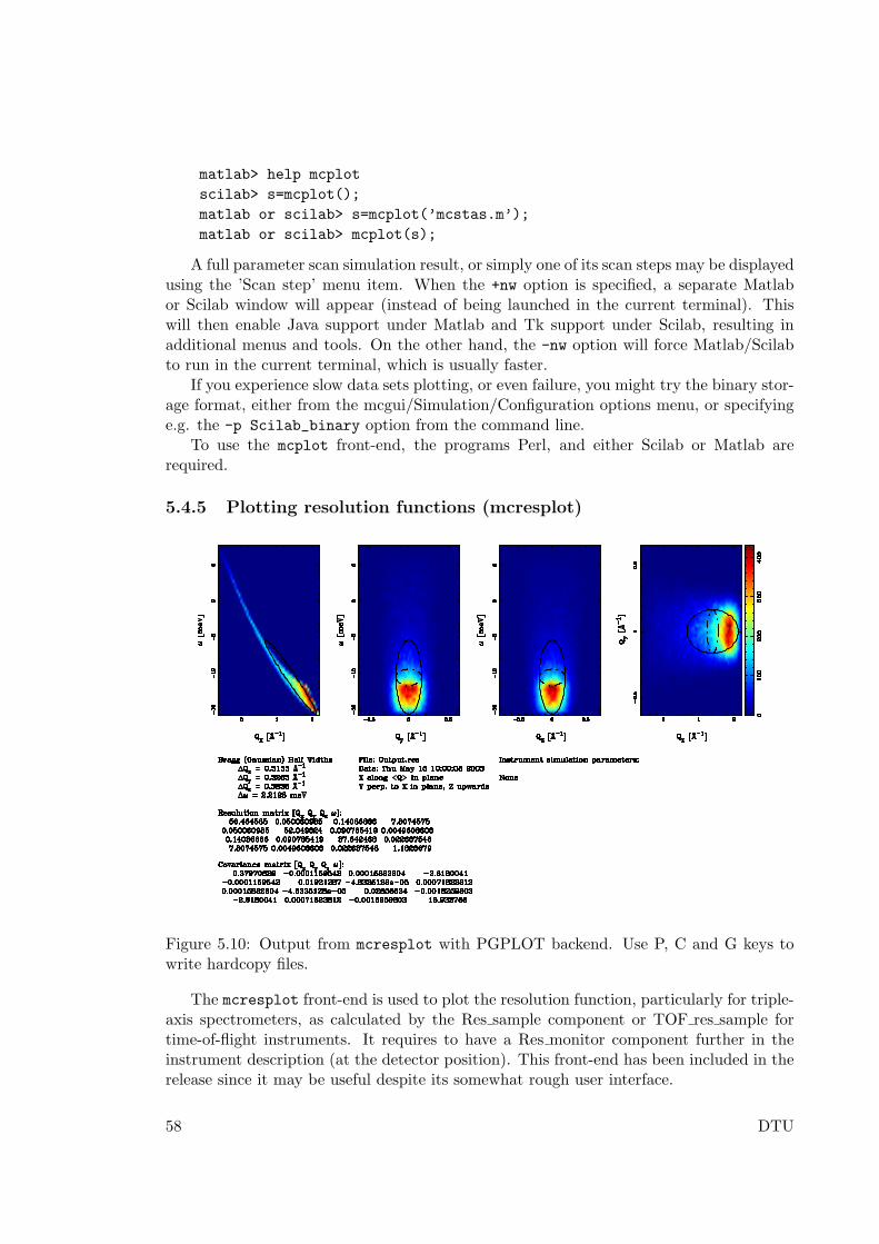
matlab> help mcplot

scilab> s=mcplot();

matlab or scilab> s=mcplot(’mcstas.m’);

matlab or scilab> mcplot(s);

A full parameter scan simulation result, or simply one of its scan steps may be displayedusing the ’Scan step’ menu item. When the +nw option is specified, a separate Matlabor Scilab window will appear (instead of being launched in the current terminal). Thiswill then enable Java support under Matlab and Tk support under Scilab, resulting inadditional menus and tools. On the other hand, the -nw option will force Matlab/Scilabto run in the current terminal, which is usually faster.

If you experience slow data sets plotting, or even failure, you might try the binary stor-age format, either from the mcgui/Simulation/Configuration options menu, or specifyinge.g. the -p Scilab_binary option from the command line.

To use the mcplot front-end, the programs Perl, and either Scilab or Matlab arerequired.

5.4.5 Plotting resolution functions (mcresplot)

Figure 5.10: Output from mcresplot with PGPLOT backend. Use P, C and G keys towrite hardcopy files.

The mcresplot front-end is used to plot the resolution function, particularly for triple-axis spectrometers, as calculated by the Res sample component or TOF res sample fortime-of-flight instruments. It requires to have a Res monitor component further in theinstrument description (at the detector position). This front-end has been included in therelease since it may be useful despite its somewhat rough user interface.

58 DTU

The mcresplot front-end is launched with the command

mcresplot file

Here, file is the name of a file output from a simulation using the Res monitor component.This front-end currently only works with the PGPLOT plotter, but ports for Matlab

and Scilab may be written in the future.The front-end will open a window displaying projections of the 4-dimensional resolution

function R(Q, ω), measured at a particular choice of Q and ω, see the component manual.The covariance matrix of the resolution function, the resolution along each projection axisand the resulting resolution matrix are also shown, as well as the instrument name andparameters used for the simulation.

To use the mcresplot front-end, the programs Perl, PGPLOT, PgPerl, and PDL mustall be properly installed on the system.

5.4.6 Creating and viewing the library, component/instrument help andManuals (mcdoc)

McStas provides an easy way to generate automatically an HTML help page about a givencomponent or instrument, or the whole McStas library.

mcdoc

mcdoc comp—instrmcdoc --tools

The first example generates an index.html catalog file using the available components andinstruments (both locally, and in the McStas library). The library catalog of componentsis opened using the BROWSER environment variable (e.g. netscape, konqueror, nautilus,MSIE, mozilla, . . . ). If the BROWSER is not defined, the help is displayed as text in thecurrent terminal. This latter output may be forced with the -t or --text option.

Alternatively, if a component or instrument comp is specified as in the second example,it will be searched within the library, and an HTML help will be created for all availablecomponents matching comp.

The last example will list the name and description of all McStas tools.Additionally, the options --web, --manual and --comp will open the McStas web site

page, the User Manual (this document) and the Component Manual, all requiring BROWSERto be defined. Finally, the --help option will display the command help, as usual.

See section 6.7 for more details about the McDoc usage and header format. To usethe mcdoc front-end, the program Perl should be available.

5.4.7 Translating McStas components for Vitess (mcstas2vitess)

Any McStas component may be translated for usage with Vitess (starting from Vitessversion 2.3). The syntax is simply

mcstas2vitess Compo.comp

This will create a Vitess module of the given component.Let us assume the component Compo shall be translated. The tool first creates a small

instrument called McStas_Compo.instr consisting of

DTU 59

1. component Vitess input

2. component Compo

3. component Vitess output

This file is parsed to generate the C file McStas_Compo.c. The last step is to compilethe C-file and build the executable Vitess module McStas_compo. For both steps McStasis used as for any other instrument. McStas_compo has to be moved to the directory’MODULES’ that contains all VITESS executables.

Additionally, a file McStas_compo.tcl is created that contains (most of) what is neededto get a GUI window in VITESS. To obtain that, the content of this file has to addedinto ’vitess.tcl’. To make it accessible within the given GUI structure of VITESS, it isnecessary to add the name ’compo’ - NO capital letters ! - to one of the folders in ’procmakeModuleSets’ (beginning of ’vitess.tcl’).

The component Virtual input transfers all neutron parameters to the McStas definitionof the co-ordinate system and the units used. (Of course Virtual output transfers it back.)This means that ’Compo’ works with the McStas definition of co-ordinate system andunits, while it is used as a VITESS module. Be careful with axis labelling.

The original parameters of the component and its position have to be given. The originof this shift is the centre of the end of the previous module, (as it is always the case inVITESS).

It is important to notice that, as VITESS uses the standard output stream (stdout) tosend neutron events, all information printed to screen must use the error stream stderr,so that all printf(...) and fprintf(stdout, ...) occurrences should be changed man-ually into fprintf(stderr, ...).

To use the mcstas2vitess front-end, the program Perl should be available.

5.4.8 Translating McStas results files between Matlab and Scilab for-mats

If you have been running a McStas simulation with Scilab output, but finally plan to lookat the results with Matlab, or the contrary, you may use

mcconvert file.m—sci

to simply translate one file format to the other. This works only for text files of course.The binary files need not be translated.

5.4.9 Translating and merging McStas results files (all text formats)

If you have been running a McStas simulation with a given text format output, but finallyplan to look at the results with an other plotter (e.g. you ran a simulation with PGPLOToutput and want to view it using Matlab), you may use

mcformat file — dir -d target dir --format=TARGET FORMAT

to translate files into format TARGET FORMAT. When given a directory, the translationworks recursively. The conversion works only for text files. Some problems may be foundwhen translating from HTML/VRML data files, or from binary files.

60 DTU

The --merge option may be used to merge similar files, e.g. obtained from grid systems,just as if a longer run was achieved.

The --scan option may be used to reconstruct the scan data from a set of direc-tories which vary by instrument parameters. For instance, you ran a scan, but finallyrealised you should have prolonged it. Then simply simulate the missing bits, and ap-ply mcformat -d scan_data --format=PGPLOT --scan step0 .. stepN. The resultingscan data is compatible with mcplot only when generating PGPLOT/McStas format. Youmay conjugate this option with the --merge in order to add/merge similar data sets beforere-building the scan.

The data files are analyzed by searching keywords inside data files (e.g. ’Source’ forthe source instrument description file). If some filenames or component names matchthese keywords (e.g. using a file ’Source.psd’), the extracted metadata information maybe wrong, even though the data itself will be correct.

5.5 Data formats - Analyzing and visualizing the simulationresults

To analyze simulation results, one uses the same tools as for analyzing experimental data,i.e. programs such as IDL, Matlab and Scilab. The output files from simulations areusually simple text files containing headers and data blocks. If data blocks are empty theymay be accessed referring to an external file indicated in the header. This file may also bea binary file (except with the original McStas/PGPLOT format), which does not containany header (except if simulation is launched with +a option), but are in turn smaller insize and faster to import.

Each data file contains informations about the simulation, the instrument, the param-eters used, and of course the signal, the estimated error on the signal, and the numberof events used in each bin. Additionally, all data files indicate their first moment (meanvalue) and second moment (half width) in the ’statistics’ field.

In order for the user to choose the data format, we recommend to set it using the--format=FORMAT or alternatively via the MCSTAS FORMAT environment variable, whichwill also make the front-end programs able to import and plot data and instrument con-sistently (see Section 5.3). The available format list is shown in Table 5.3.

Note that the neutron event counts in detectors are typically not very meaningfulexcept as a way to measure the performance of the simulation. Use the simulated intensityinstead whenever analysing simulation data.

5.5.1 McStas and PGPLOT format

The McStas original format, which is equivalent to the PGPLOT format, is simply columnsof ASCII text that most programs should be able to read.

One-dimensional histogram monitors (time-of-flight, energy) write one line for eachhistogram bin. Each line contains a number identifying the bin (i.e. the time-of-flight)followed by three numbers: the simulated intensity, an estimate of the statistical error asexplained in section 4.2.1, and the number of neutron events for this bin.

Two-dimensional histogram monitors (position sensitive detectors) output M lines ofN numbers representing neutron intensities, where M and N are the number of bins in the

DTU 61

two dimensions. The two-dimensional monitors also store the error estimates and eventcounts as additional matrices.

Single-point monitors output the neutron intensity, the estimated error, and the neu-tron event count as numbers on the terminal. (The results from a series of simulationsmay be combined in a data file using the mcrun front-end as explained in section 5.4.2).

When using one- and two-dimensional monitors, the integrated intensities are writtento terminal as for the single-point monitor type, supplementing file output of the full one-or two-dimensional intensity distribution. Both one- and two-dimensional monitor outputby default start with a header of comment lines, all beginning with the ‘#’ character. Thisheader gives such information as the name of the instrument used in the simulation, thevalues of any instrument parameters, the name of the monitor component for this datafile, etc. The headers may be disabled using the --data-only option in case the file mustbe read by a program that cannot handle the headers.

In addition to the files written for each one- and two-dimensional monitor component,another file (by default named mcstas.sim) is also created. This file is in a specialMcStas ASCII format. It contains all available information about the instrument definitionused for the simulation, the parameters and options used to run the simulation, and themonitor components present in the instrument. It is read by the mcplot front-end (seesection 5.4.4). This file stores the results from single monitors, but by default containsonly pointers (in the form of file names) to data for one- and two-dimensional monitors.By storing data in separate files, reading the data with programs that do not know thespecial McStas file format is simplified. The --file option may be used to store all datainside the mcstas.sim file instead of in separate files.

5.5.2 Matlab, Scilab and IDL formats

With these formats McStas automatically writes scripts containing the data as a structure,as well as in-line import and plot functions for the selected language. Usage examples aregiven in section 5.3. Thus, it is not necessary to write a load routine for each format,as the script is itself a program that knows how to handle the data. Alternatively, usingmcplot with Matlab and Scilab plotters provide additional functionalities from menus anddialogs (see section 5.4.4).

When imported through the data generated script (see section 5.3), or using mcplot

(see section 5.4.4), a single variable may be created into the Matlab, Scilab or IDL baseworkspace. This variable is a structure constituting a data tree containing many fields,some being themselves structures. Field names are the initial names from the instrument(components, files, . . . ), transformed into valid variable names, e.g containing only letters,digits and the ’ ’ character, except for the first character which may only be a letter.When using Matlab, an ’m ’ is appended to avoid name clash with existing Matlab com-mands/variables.1. In this tree, you will find the monitor names, which fields contain themonitored data. The usual structure is

s.instrument.simulation.comp name.file name

For instance, reading the data from a ’test’ instrument using Matlab format will looklike

1For instance in most case, the simulation location is ’./mcstas.m’ which turns into field ’m mcstas’.

62 DTU

matlab> s=mcstas; % or mcplot mcstas.m from the terminal

matlab> s

s =

Format: ’Matlab with text headers’

URL: ’http://neutron.risoe.dk’

Editor: ’farhi on pcfarhi’

Creator: ’test (test.instr) McStas 1.9 - Nov. 15, 2005 simulation’

Date: 1.0529e+09

File: ’./mcstas’

test: [1x1 struct]

EndDate: 1.0529e+09

class: ’root’

matlab> s.test.m_mcstas.monitor1.monitor1_y_kz

ans =

...

Date: 1.0529e+09

File: ’monitor1.y_kz’

type: ’array_2d(20, 10)’

...

ratio: ’1e+06/1e+06’

signal: ’Min=0; Max=5.54051e-10; Mean= 6.73026e-13;’

statistics: ’X0=0.438302; dX=0.0201232; Y0=51019.6; dY=20557.1;’

...

matlab> eval(s.test.m_mcstas.monitor1.monitor1_y_kz);

matlab> dX

ans =

0.0201232

The latter example accesses the data from the ’monitor1.y kz’ file written by the ’monitor1’component in the ’test’ instrument during the ’./mcstas’ simulation. You may evaluatedirectly the ’signal’ and ’statistics’ fields of the structure to obtain useful information.

5.5.3 HTML/VRML and XML formats

Both HTML and XML formats are available. The former may be viewed using any webbrowser (Netscape/Mozilla/Firefox, Internet Explorer, Nautilus, Konqueror) - showingdata sets as VRML objects. XML data sets may be browsed for instance using InternetExplorer (Windows and Mac OS) or Firefox, GXMLViewer and KXMLEditor (underLinux).

The XML format is NeXus-like, but not fully compatible. However, McStas maygenerate genuine NeXus/HDF format (see bellow).

5.5.4 NeXus format

The NeXus format [47] is a platform independent HDF binary data file. To have McStasuse it

1. the HDF and NeXus libraries must have been installed

DTU 63

2. the McStas installation should be done with NeXus bindings, e.g. on Unix/Linuxsystems configure --with-nexus; make; make install.

3. the compilation of instruments must be done with the -DHUSE_NEXUS -lNeXus flag(see Section 6.3.4). This is automated with the mcrun tool (Section 5.4.2).

All results are saved in a single file, containing ’groups’ of data. To view such files,install and use HDFView (or alternatively HDFExplorer). This Java viewer can showcontent of all detectors, including metadata (attributes). Basic detector images may alsobe generated.

5.6 Using computer Grids and Clusters

Parallelizing a computation is in general possible when dependencies between each com-putation are not too strong. The situation of McStas is ideal since each neutron ray can besimulated without interfering with other simulated neutron rays. Therefore each neutronray can be simulated independently on a set of computers.

When computing N neutron rays with p computers, each computer will simulate Np

neutrons. As a result there will be p · Np = N neutrons simulated. As a result, McStas

generates two kinds of data sets:

• intensity measurements, internally represented by three values (p0, p1, p2) where p0,p1, p2 are additive. Therefore the final value of p0 is the sum of all local value ofp0 computed on each node. The same rule applies for p1 and p2. The evaluation ofthe intensity errors σ is performed using the final p0, p1, and p2 arrays (see Section4.2.1).

• event lists: the merge of events is done by concatenation

McStas provides three methods in order to distribute computations on many comput-ers.

• when using a set of nodes (grid, cluster or multi-cores), it is possible to distributesimulations on a list of computers and multi-core machines (see section 5.6.1). Re-sults are automatically merged after completion. This method is very efficient, andonly requires SSH server to be installed/configured on slave machines. In order touse an heterogeneous system, a C compiler should be optionally installed on slavemachines.

• when using an homogeneous computer cluster, each simulation (including scan steps)may be computed in parallel using MPI. We recommend this method on clusters (seesection 5.6.2).

Last but not least, you may run simulations manually on a number of machines.Once the distributed simulation have been completed, you may merge their results usingmcformat (see section 5.4.9) in order to obtain a set of files just as if it had been executedon a single machine.

All of these methods can be used, when available, from mcgui.

64 DTU

5.6.1 Distribute mcrun simulations on grids, multi-cores and clusters(SSH grid)

This method distributes simulations on a set of machines using ssh connections, using acommand such as mcrun --grid=4 .... Each of the scan steps is split and executed ondistant slave machines, sending the executable with scp, executing single simulations, andthen retrieving individual results on the master machine. These are then merged usingmcformat.

The mcrun script has been adapted to use transparently SSH grids. The syntax is:

• --grid=<number>: tells mcrun to use the grid over <number> nodes.

• --machines=<file>: defines a text file where the nodes which are to be used forparallel computation are listed; by default, mcrun will look at $HOME/.mcstas-hostsand MCSTAS/tools/perl/mcstas-hosts. When used on a single SMP machine(multi-core/cpu), this option may be omitted.

• --force-compile: this option is required on heterogeneous systems. The C code issent to all slaves and simulation is compiled on each node before starting computa-tion. The default is to send directly the executatble from the master node, whichonly works on homogeneous systems. computation.

This method shows similar efficiency as MPI, but without MPI installation. It isespecially suited on multi-core machines, but may also be used on any set of distantmachines (grids), as well as clusters. For Windows master machines, we recommend theinstallation of the PuTTY SSH client. The overhead is proportional to the number ofnodes and the amount of data files to transfer per simulation. It is usually larger than thepure MPI method. We thus recommend to launch long runs on fewer nodes rather thanmany short runs on many nodes.

Requirements and limitation (SSH grids)

1. A master machine with an SSH client, and McStas installation.

2. A set of machines (homogeneous or heterogeneous) with SSH servers.

3. On heterogeneous grids, a C compiler must also be installed on all slave nodes.

4. ssh access from the master node (where McStas is installed) to the slaves through e.g.DSA keys without a password. These keys should be generated using the commandssh-keygen. Run e.g. ssh-keygen -t dsa on master node, enter no passphrase andadd resulting .ssh/id dsa.pub to .ssh/authorized keys on all the slave nodes.The key generation and registering mechanism may be done automatically for thelocal machine from the Help menu/Install DSA key item of mcgui.

5. The machine names listed in the file .mcstas-hosts in your home directory or inthe MCSTAS/tools/perl/mcstas-hosts on the master node, one node per line. The--machines=<file> option enables to specify the hosts file to use. If it does notexist, only the current machine will be used (for multi-processor/core machines).

DTU 65

6. Without ssh keys, passwords will be prompted many times. To avoid this, we recom-mend to use only the local machine (for multi-cores/cpu), i.e. do not use a machinehosts file.

7. If your simulation/instrument requires data files (Powders, Sqw, source description,...), these must be copied at the same level as the instrument definition. They aresent to all slave nodes before starting each computation. Take care to limit as muchas possible the required data file volume in order to avoid large data transfers.

8. Interrupting or sending Signals may fail during computations. However, simulationscans can be interrupted as soon as the on-going computation step ends.

9. With heterogeneous systems, we recommend to use the mcrun --force-compile

command rather than McGUI, which may skip the required simulation compilationon slaves.

5.6.2 Parallel computing (MPI)

The MPI support requires that MPICH (recommended), or alternatively LAM-MPI orOpenMPI, is installed on a set of nodes. This usually also requires properly setup ssh

connections and keys as indicated in the ssh grid system (Section 5.6.1). Some OpenMPIimplementations do not recognise multi-cores as separate nodes. In this case, you shoulduse MPICH, or the SSH grid.

There are 3 methods for using MPI

• Basic usage requires to compile and run the simulation by hand (mpicc, mpirun).This should be used when running LAM-MPI.

• A much simpler way is to use mcrun -c --mpi=NB_CPU ... which will recompileand run MPICH.

• The McGUI interface supports MPICH from within the Run Dialog.

The MPI support is especially suited on clusters. As an alternative, the SSH gridpresented above (section 5.6.1) is very flexible and requires lighter configuration.

Requirements and limitation (MPI)

To use MPI you will need

1. A master machine with an SSH client/server, and McStas installation.

2. A set of unix machines of the same architecture (binary compatible) with SSHservers.

3. ssh access from the master node (where McStas is installed) to the slaves through e.g.DSA keys without a password. These keys should be generated using the commandssh-keygen. Run e.g. ssh-keygen -t dsa on master node, enter no passphrase andadd resulting .ssh/id dsa.pub to .ssh/authorized keys on all the slave nodes.The key generation and registering mechanism may be done automatically for thelocal machine from the Help menu/Install DSA key item of mcgui.

66 DTU

4. The machine names listed in the file .mcstas-hosts in your home directory or inthe MCSTAS/tools/perl/mcstas-hosts on the master node, one node per line. The--machines=<file> option enables to specify the hosts file to use. If it does notexist, only the current machine will be used (for multi-processor/core machines).

5. Without ssh keys, passwords will be prompted many times. To avoid this, we recom-mend to use only the local machine (for multi-cores/cpu), i.e. do not use a machinehosts file.

6. Signals are not supported while simulating with MPI (since asynchronous eventscannot be easily transmitted to all nodes). This means it is not possible to cancelan on-going computation. However, simulation scans can be interrupted as soon asthe on-going computation step ends.

7. MPI must be correctly configured: if using ssh, you have to set ssh keys to avoid useof passwords; if using rsh, you have to set a .rhosts file. On non-local accounts,this procedure may fail and ssh always require passwords.

MPI Basic usage

To enable parallel computation, compile McStas output C-source file with mpicc with theflag -DUSE_MPI and run it using the wrapper of your MPI implementation (mpirun formpich or lammpi) :

# generate a C-source file [sim.c]

mcstas sim.instr

# generate an executable with MPI support [sim.mpi]

mpicc -DUSE_MPI -o sim.mpi sim.c

# execute with parallel processing over <N> computers

# here you have to list the computers you want to use

# in a file [machines.list] (using mpich implementation)

# (refer to MPI documentation for a complete description)

mpirun -machinefile machines.list -n <N> \

./sim.mpi <instrument parameters>

...

If you don’t want to spread the simulation, run it as usual :

./sim.mpi <instrument parameters>

5.6.3 McRun script with MPI support (mpich)

The mcrun script has been adapted to use MPICH implementation of MPI. Two newoptions have been added:

• --mpi=<number>: tells mcrun to use MPI, and to spread the simulation over <number>nodes

DTU 67

• --machines=<file>: defines a text file where the nodes which are to be used forparallel computation are listed; by default, mcrun will look at $HOME/.mcstas-hostsand MCSTAS/tools/perl/mcstas-hosts. When used on a single SMP machine(multi-core/cpu), this option may be omitted.

When available, the MPI option will show up in the mcgui Run dialog. Specify the numberof nodes required.

Suppose you have four machines named node1 to node4. A typical machine list file,machines.list looks like :

node1

node2

node3

node4

You can then spread a simulation sim.instr using mcrun :

mcrun -c --mpi=4 --machines=machines.list \

sim.instr <instrument parameters>

Warning: when using mcrun with MPI, be sure to recompile your simulation with MPIsupport (see -c flag of mcrun): a simulation compiled without MPI support cannot beused with MPI, whereas a simulation compiled with MPI support can be used withoutMPI.

5.6.4 McStas/MPI Performance

Theoretically, a computation which lasts T seconds on a single computer, should lasts atleast T

p seconds when it is distributed over p computers. In practice, there will be overheadtime due to the split and merge operations.

• the split is immediate: constant time cost O(1)

• the merge is at worst linear against the number of computers:

– linear time cost : O(p) when saving an event list

– logarithmic time cost: O(log p) when not saving an event list

The efficiency of McStas using MPI has been tested on large clusters, up to 500 nodes.The computation time decreases in the same proportion as the number of nodes, showingan ideal efficiency. However, a small overhead may appear depending on the clusterinternal network load, which may be estimated at most of about 10-20 s. This overheadcomes from the spread and the fusion of the computations. For instance, spreading acomputation implies often an rsh or and ssh session to be opened on every node. Toreach the best efficiency, the computation time should not be lower than 30 seconds, orthe overhead time may become significant compared to total time.

68 DTU

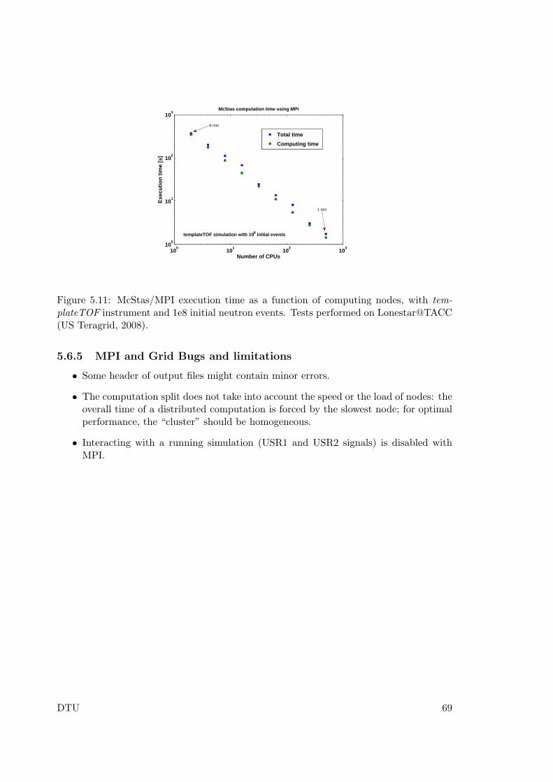
100

101

102

103

100

101

102

103

Number of CPUs

Exe

cuti

on

tim

e [s

]

McStas computation time using MPI

templateTOF simulation with 108 initial events

Total time

Computing time

6 min

1 sec

Figure 5.11: McStas/MPI execution time as a function of computing nodes, with tem-plateTOF instrument and 1e8 initial neutron events. Tests performed on Lonestar@TACC(US Teragrid, 2008).

5.6.5 MPI and Grid Bugs and limitations

• Some header of output files might contain minor errors.

• The computation split does not take into account the speed or the load of nodes: theoverall time of a distributed computation is forced by the slowest node; for optimalperformance, the “cluster” should be homogeneous.

• Interacting with a running simulation (USR1 and USR2 signals) is disabled withMPI.

DTU 69

Chapter 6

The McStas kernel andmeta-language

Instrument definitions are written in a special McStas meta-language which is translatedautomatically by the McStas compiler into a C program which is in turn compiled toan executable that performs the simulation. The meta-language is custom-designed forneutron scattering and serves two main purposes: (i) to specify the interaction of a singleneutron ray with a single optical component, and (ii) to build a simulation by constructinga complete instrument from individual components.

For maximum flexibility and efficiency, the meta-language is based on C. Instrumentgeometry, propagation of neutrons between the different components, parameters, datainput/output etc. is handled in the meta-language and by the McStas compiler. Complexcalculations are written in C embedded in the meta-language description of the compo-nents. However, it is possible to set up an instrument from existing components and run asimulation without writing a single line of C code, working entirely in the meta-language.

Apart from the meta-language, McStas also includes a number of C library functionsand definitions that are useful for neutron ray-tracing simulations. The definitions avail-able for component developers are listed in appendix B. The list includes functions for

• Computing the intersection between a flight-path and various objects (such as planes,cylinders, boxes and spheres)

• Functions for generating random numbers with various distributions

• Functions for reading or writing information from/to data files

• Convenient conversion factors between relevant units, etc.

The McStas meta-language was designed to be readable, with a verbose syntax and ex-plicit mentioning of otherwise implicit information. The recommended way to get startedwith the meta-language is to start by looking at the examples supplied with McStas,modifying them as necessary for the application at hand.

70 DTU

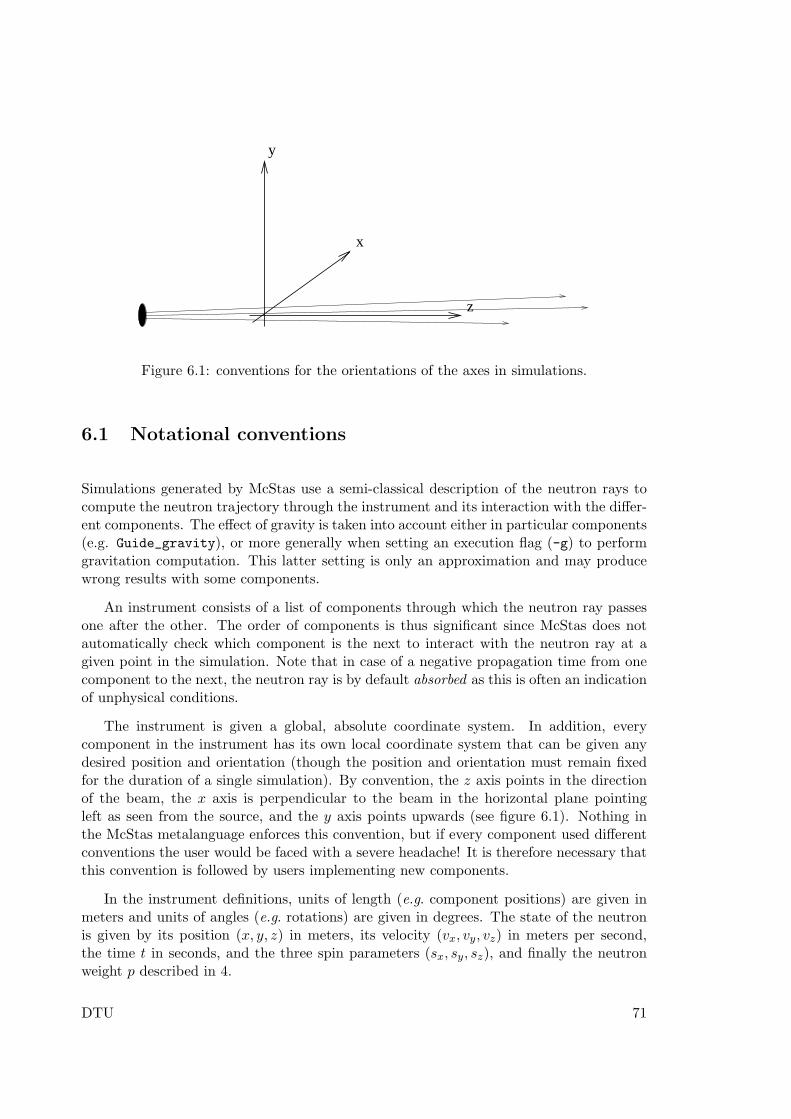
z

x

y

Figure 6.1: conventions for the orientations of the axes in simulations.

6.1 Notational conventions

Simulations generated by McStas use a semi-classical description of the neutron rays tocompute the neutron trajectory through the instrument and its interaction with the differ-ent components. The effect of gravity is taken into account either in particular components(e.g. Guide_gravity), or more generally when setting an execution flag (-g) to performgravitation computation. This latter setting is only an approximation and may producewrong results with some components.

An instrument consists of a list of components through which the neutron ray passesone after the other. The order of components is thus significant since McStas does notautomatically check which component is the next to interact with the neutron ray at agiven point in the simulation. Note that in case of a negative propagation time from onecomponent to the next, the neutron ray is by default absorbed as this is often an indicationof unphysical conditions.

The instrument is given a global, absolute coordinate system. In addition, everycomponent in the instrument has its own local coordinate system that can be given anydesired position and orientation (though the position and orientation must remain fixedfor the duration of a single simulation). By convention, the z axis points in the directionof the beam, the x axis is perpendicular to the beam in the horizontal plane pointingleft as seen from the source, and the y axis points upwards (see figure 6.1). Nothing inthe McStas metalanguage enforces this convention, but if every component used differentconventions the user would be faced with a severe headache! It is therefore necessary thatthis convention is followed by users implementing new components.

In the instrument definitions, units of length (e.g. component positions) are given inmeters and units of angles (e.g. rotations) are given in degrees. The state of the neutronis given by its position (x, y, z) in meters, its velocity (vx, vy, vz) in meters per second,the time t in seconds, and the three spin parameters (sx, sy, sz), and finally the neutronweight p described in 4.

DTU 71

6.2 Syntactical conventions

Comments follow the normal C syntax “/* ... */”. C++ style comments “// ...” mayalso be used.

Keywords are not case-sensitive, for example “DEFINE”, “define”, and “dEfInE” are allequivalent. However, by convention we always write keywords in uppercase to distinguishthem from identifiers and C language keywords. In contrast, McStas identifiers (names),like C identifiers and keywords, are case sensitive, another good reason to use a consistentcase convention for keywords. All McStas keywords are reserved, and thus should not beused as C variable names. The list of these reserved keywords is shown in table 6.1.

It is possible, and usual, to split the input instrument definition across several differentfiles. For example, if a component is not explicitly defined in the instrument, McStas willsearch for a file containing the component definition in the standard component library (aswell as in the current directory and any user-specified search directories, see section 5.2.2).It is also possible to explicitly include another file using a line of the form

%include "file"

Beware of possible confusion with the C language “#include” statement, especially whenit is used in C code embedded within the McStas meta-language. Files referenced with“%include” are read when the instrument is translated into C by the McStas compiler, andmust contain valid McStas meta-language input (and possibly C code). Files referencedwith “#include” are read when the C compiler generates an executable from the generatedC code, and must contain valid C.

Embedded C code is used in several instances in the McStas meta-language. Such codeis copied by the McStas compiler into the generated simulation C program. Embedded Ccode is written by putting it between the special symbols % and %, as follows:

%

. . . Embedded C code . . .%

The “%” and “%” must appear on a line by themselves (do not add comments after).Additionally, if a “%include” statement is found within an embedded C code block, thespecified file will be included from the ’share’ directory of the standard component library(or from the current directory and any user-specified search directories) as a C library,just like the usual “#include” but only once. For instance, if many components requireto read data from a file, they may all ask for “%include "read_table-lib"” withoutduplicating the code of this library. If the file has no extension, both .h and .c files willbe searched and included, otherwise, only the specified file will be imported. The McStas’run-time’ shared library is included by default (equivalent to “%include "mcstas-r"”in the DECLARE section). For an example of %include, see the monitors/Monitor nDcomponent. See also section 6.4 for insertion of full instruments in instruments (instrumentconcatenation).

If the instrument description compilation fails, check that the keywords syntax is cor-rect, that no semi-colon ; sign is missing (e.g. in C blocks and after an ABSORB macro),and there are no name conflicts between instrument and component instances variables.

72 DTU

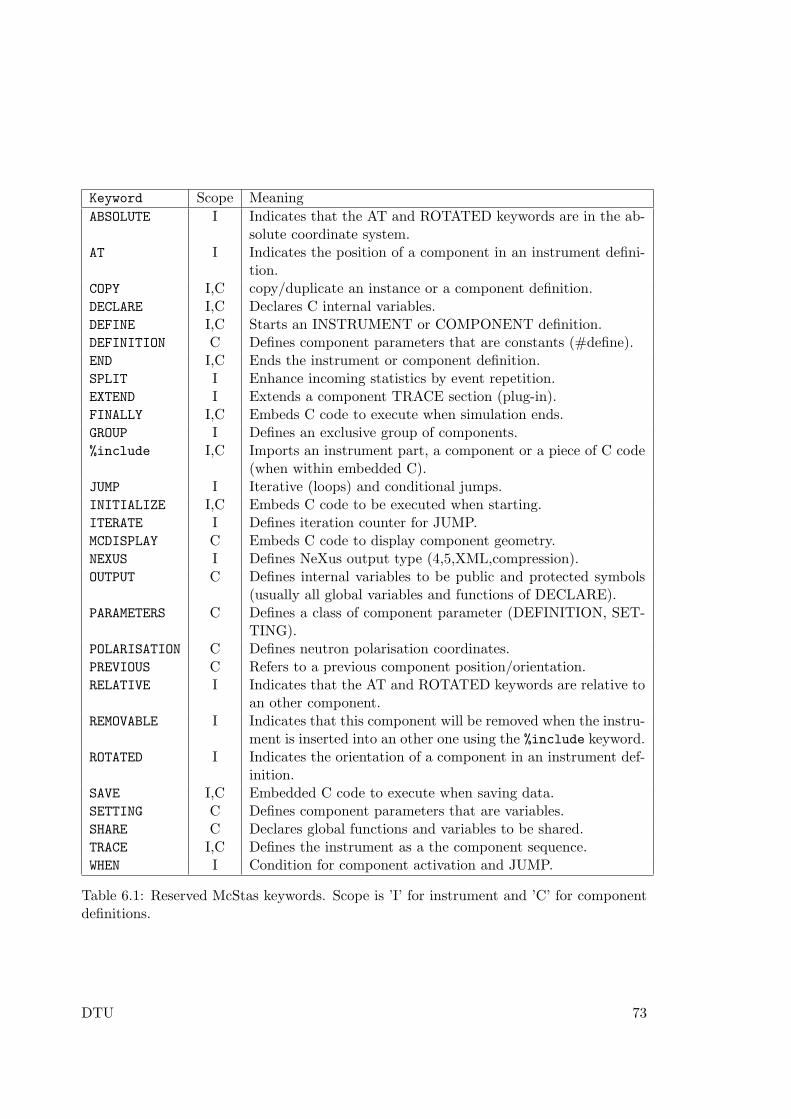
Keyword Scope Meaning

ABSOLUTE I Indicates that the AT and ROTATED keywords are in the ab-solute coordinate system.

AT I Indicates the position of a component in an instrument defini-tion.

COPY I,C copy/duplicate an instance or a component definition.DECLARE I,C Declares C internal variables.DEFINE I,C Starts an INSTRUMENT or COMPONENT definition.DEFINITION C Defines component parameters that are constants (#define).END I,C Ends the instrument or component definition.SPLIT I Enhance incoming statistics by event repetition.EXTEND I Extends a component TRACE section (plug-in).FINALLY I,C Embeds C code to execute when simulation ends.GROUP I Defines an exclusive group of components.%include I,C Imports an instrument part, a component or a piece of C code

(when within embedded C).JUMP I Iterative (loops) and conditional jumps.INITIALIZE I,C Embeds C code to be executed when starting.ITERATE I Defines iteration counter for JUMP.MCDISPLAY C Embeds C code to display component geometry.NEXUS I Defines NeXus output type (4,5,XML,compression).OUTPUT C Defines internal variables to be public and protected symbols

(usually all global variables and functions of DECLARE).PARAMETERS C Defines a class of component parameter (DEFINITION, SET-

TING).POLARISATION C Defines neutron polarisation coordinates.PREVIOUS C Refers to a previous component position/orientation.RELATIVE I Indicates that the AT and ROTATED keywords are relative to

an other component.REMOVABLE I Indicates that this component will be removed when the instru-

ment is inserted into an other one using the %include keyword.ROTATED I Indicates the orientation of a component in an instrument def-

inition.SAVE I,C Embedded C code to execute when saving data.SETTING C Defines component parameters that are variables.SHARE C Declares global functions and variables to be shared.TRACE I,C Defines the instrument as a the component sequence.WHEN I Condition for component activation and JUMP.

Table 6.1: Reserved McStas keywords. Scope is ’I’ for instrument and ’C’ for componentdefinitions.

DTU 73

6.3 Writing instrument definitions

The purpose of the instrument definition is to specify a sequence of components, along withtheir position and parameters, which together make up an instrument. Each componentis given its own local coordinate system, the position and orientation of which may bespecified by its translation and rotation relative to another component. An example isgiven in section 6.3.9 and some additional examples of instrument definitions can be foundon the McStas web-page [2] and in the example directory.

As a summary, the usual grammar for instrument descriptions is

DEFINE INSTRUMENT name(parameters)

DECLARE C_code

INITIALIZE C_code NEXUS

TRACE components

FINALLY C_code

END

6.3.1 The instrument definition head

DEFINE INSTRUMENT name (a1, a2, . . .)

This marks the beginning of the definition. It also gives the name of the instrumentand the list of instrument parameters. Instrument parameters describe the configurationof the instrument, and usually correspond to setting parameters of the components, seesection 6.5. A motor position is a typical example of an instrument parameter. The inputparameters of the instrument constitute the input that the user (or possibly a front-endprogram) must supply when the generated simulation is started.

By default, the parameters will be floating point numbers, and will have the C typedouble (double precision floating point). The type of each parameter may optionally bedeclared to be int for the C integer type or char * for the C string type. The name stringmay be used as a synonym for char *, and floating point parameters may be explicitlydeclared using the name double. The following example illustrates all possibilities:

DEFINE INSTRUMENT test(d1, double d2, int i, char *s1, string s2)

Here d1 and d2 will be floating point parameters of C type double, i will be an integerparameter of C type int, and s1 and s2 will be string parameters of C type char *.The parameters of an instrument may be given default values. Parameters with defaultvalues are called optional parameters, and need not be given an explicit value when theinstrument simulation is executed. When executed without any parameter value in thecommand line (see section 5.3), the instrument asks for all parameter values, but pressingthe Return key selects the default value (if any). When used with at least one parametervalue in the command line, all non specified parameters will have their value set to thedefault one (if any). A parameter is given a default value using the syntax “param=

value”. For example

DEFINE INSTRUMENT test(d1= 1, string s2="hello")

74 DTU

Here d1 and d2 are optional parameters and if no value are given explicitly, “1” and “hello”will be used.

Optional parameters can greatly increase the convenience for users of instruments forwhich some parameters are seldom changed or of unclear signification to the user. Also,if all instrument parameters have default values, then the simple command mcdisplay

test.instr will show the instrument view without requesting any other input, which isusually a good starting point to study the instrument design.

6.3.2 The DECLARE section

DECLARE

%

. . . C declarations of global variables etc. . . .%

This gives C declarations that may be referred to in the rest of the instrument definition. Atypical use is to declare global variables or small functions that are used elsewhere in the in-strument. The %include ’’file’’ keyword may be used to import a specific componentdefinition or a part of an instrument. Variables defined here are global, and may con-flict with internal McStas variables, specially symbols like x,y,z,sx,sy,sz,vx,vy,vz,t

and generally all names starting with mc should be avoided. If you can not compile theinstrument, this may be the reason. The DECLARE section is optional.

6.3.3 The INITIALIZE section

INITIALIZE

%

. . . C initializations. . . .%

This gives code that is executed when the simulation starts. This section is optional. In-strument setting parameters may be modified in this section (e.g. doing tests or automaticsettings).

6.3.4 The NEXUS extension

The NeXus format [47] requires to link the simulation to additional libraries (HDF andNeXus) which must have been pre-installed. Preferably, McStas should have been installedwith the ./configure --with-nexus on Unix/Linux systems. To activate the NeXusoutput, the compilation of the instrument must be done with flag -DUSE_NEXUS -lNeXus.The resulting executable is no longer portable.

The default NeXus format is NeXus 5 with compression. However, that format maybe changed with the optional keyword NEXUS to follow the INITIALIZE section, namely:

INITIALIZE

%

. . . C initializations. . . .% NEXUS "4"|"5"|"XML"|"compress"|"zip"

DTU 75

It is possible to set the type of NeXus file with a string argument, containing words ”4”,”5” or ”XML”. Optionally, if the string also contains the compress or zip word, the NeXusfile will use compression for Data Sets. We recommend the syntax NEXUS "5 compress"

which is the default.You may choose the name of the output file with the -f filename option from the

instrument executable or mcrun (see Sections 5.3, 5.4.2 and Table 5.2).Then, the output format is chosen as usual with the --format=NeXus option when

launching the simulation. All output files are stored in the output filename, as well asthe instrument description itself. Other formats are still available. When run on a dis-tributed system (e.g. MPI), detectors are gathered, but list of events (see e.g. componentVirtual output) are stored as one data set per node.

6.3.5 The TRACE section

As a summary, the usual grammar for component instances within the instrument TRACEsection is

COMPONENT name = comp(parameters)

AT (...) [RELATIVE [reference|PREVIOUS] | ABSOLUTE]

ROTATED RELATIVE [reference|PREVIOUS] | ABSOLUTE

The TRACE keyword starts a section giving the list of components that constitute theinstrument. Components are declared like this:

COMPONENT name = comp(p1 = e1, p2 = e2, . . .)

This declares a component named name that is an instance of the component definitionnamed comp. The parameter list gives the setting and definition parameters for thecomponent. The expressions e1, e2, . . . define the values of the parameters. For settingparameters arbitrary ANSI-C expressions may be used, while for definition parametersonly constant numbers, strings, names of instrument parameters, or names of C identifiersare allowed (see section 6.5.1 for details of the difference between definition and settingparameters). To assign the value of a general expression to a definition parameter, it isnecessary to declare a variable in the DECLARE section, assign the value to the variable inthe INITIALIZE section, and use the variable as the value for the parameter.

The McStas program takes care to rename parameters appropriately in the outputso that no conflicts occur between different component definitions or between componentand instrument definitions. It is thus possible (and usual) to use a component definitionmultiple times in an instrument description.

Beware about variable type conversion when setting numerical parameter values, asin p1=12/1000. In this example, the parameter p1 will be set to 0 as the division ofthe two integers is indeed 0. To avoid that, use explicitely floating type numbers as inp1=12.0/1000.

The McStas compiler will automatically search for a file containing a definition of thecomponent if it has not been declared previously. The definition is searched for in a filecalled “name.comp”. See section 5.2.2 for details on which directories are searched. Thisfacility is often used to refer to existing component definitions in standard componentlibraries. It is also possible to write component definitions in the main file before the

76 DTU

instrument definitions, or to explicitly read definitions from other files using %include

(not within embedded C blocks).

The physical position of a component is specified using an AT modifier following thecomponent declaration:

AT (x, y, z) RELATIVE name

This places the component at position (x, y, z) in the coordinate system of the previ-ously declared component name. Placement may also be absolute (not relative to anycomponent) by writing

AT (x, y, z) ABSOLUTE

Any C expression may be used for x, y, and z. The AT modifier is required. Rotation isachieved similarly by writing

ROTATED (φx, φy, φz) RELATIVE name

This will result in a coordinate system that is rotated first the angle φx (in degrees) aroundthe x axis, then φy around the y axis, and finally φz around the z axis. Rotation mayalso be specified using ABSOLUTE rather than RELATIVE. If no rotation is specified, thedefault is (0, 0, 0) using the same relative or absolute specification used in the AT modifier.We strongly recommend to apply all rotations of an instrument description on Arm classcomponents only, acting as goniometers, and position the optics on top of these. Thisusually makes it much easier to orient pieces of the instrument, and avoid positioningerrors.

The position of a component is actually the origin of its local coordinate system.Usually, this is used as the input window position (e.g. for guide-like components), or thecenter position for cylindrical/spherical components.

The PREVIOUS keyword is a generic name to refer to the previous component in thesimulation. Moreover, the PREVIOUS(n) keyword will refer to the n-th previous component,starting from the current component, so that PREVIOUS is equivalent to PREVIOUS(1).This keyword should be used after the RELATIVE keyword, but not for the first componentinstance of the instrument description.

AT (x, y, z) RELATIVE PREVIOUS ROTATED (φx, φy, φz) RELATIVE PREVIOUS(2)

Invalid PREVIOUS references will be assumed to be absolute placement.

The order and position of components in the TRACE section does not allow componentsto overlap, except for particular cases (see the GROUP keyword below). Indeed, manycomponents of the McStas library start by propagating the neutron event to the beginningof the component itself. Anyway, when the corresponding propagation time is found to benegative (i.e. the neutron ray is already after or aside the component, and has thus passedthe ’active’ position), the neutron event is ABSORBed, resulting in a zero intensity andevent counts after a given position. The number of such removed neutrons is indicated atthe end of the simulation. Getting such warning messages is an indication that either somecomponents overlap, or some neutrons are getting outside of the simulation, for instancethis usually happens after a monochromator, as the non-reflected beam is indeed lost. A

DTU 77

special warning appears when no neutron ray has reached some part of the simulation.This is usually the sign of either overlapping components or a very low intensity.

For experienced users, we recommend as well the usage of the WHEN and EXTEND key-words, as well as other syntax extensions presented in section 6.4 below.

6.3.6 The SAVE section

SAVE

%

. . . C code to execute each time a temporary save is required . . .%

This gives code that will be executed when the simulation is requested to save data, forinstance when receiving a USR2 signal (on Unix systems), or using the Progress_bar

component with intermediate savings. It is also executed when the simulation ends. Thissection is optional.

6.3.7 The FINALLY section

FINALLY

%

. . . C code to execute at end of simulation . . .%

This gives code that will be executed when the simulation has ended. When existing,the SAVE section is first executed. The FINALLY section is optional. A simulation may berequested to end before all neutrons have been traced when receiving a TERM or INTsignal (on Unix systems), or with Control-C, causing code in FINALLY to be evaluated.

6.3.8 The end of the instrument definition

The end of the instrument definition must be explicitly marked using the keyword

END

6.3.9 Code for the instrument vanadium example.instr

A commented instrument definition taken from the examples directory is here shown asan example of the use of McStas.

/*******************************************************************************

*

* McStas, neutron ray-tracing package

* Copyright (C) 1997-2008, All rights reserved

* Risoe National Laboratory, Roskilde, Denmark

* Institut Laue Langevin, Grenoble, France

*

* Instrument: Samples_vanadium

*

* %Identification

* Written by: Kristian Nielsen and Kim Lefmann

78 DTU

* Date: 1998

* Origin: Risoe

* Release: McStas CVS_080624

* Version: $Revision: 1.3 $

* %INSTRUMENT_SITE: Tests_samples

*

* A test instrument using a vanadium cylinder

*

* %Description

* This instrument shows the vanadium sample scattering anisotropy.

* This is an effect of attenuation of the beam in the cylindrical sample.

*

* %Example: ROT=0 Detector: PSD_4pi_I=7.97023e-05

*

* %Parameters

* INPUT PARAMETERS:

* ROT: (deg) Rotation angle of the PSD monitor

*

* %Link

* The McStas User manual

* The McStas tutorial

*

* %End

*******************************************************************************/

/* The line below defines the ’name’ of our instrument */

/* Here, we have a single input parameter, ROT */

DEFINE INSTRUMENT Samples_vanadium(ROT=0)

/* The DECLARE section allows us to declare variables */

/* in c syntax. Here, coll_div (collimator divergence) */

/* is set to 60 degrees... */

DECLARE

%

double coll_div = 60;

%

/* Here comes the TRACE section, where the actual */

/* instrument is defined.... */

TRACE

/* The Arm() class component defines reference points */

/* in 3D space. Every component instance must have a */

/* unique name. Here, arm is used. This Arm() component*/

/* is set to define the origin of our global coordinate*/

/* system (AT (0,0,0) ABSOLUTE) */

COMPONENT arm = Arm() AT (0,0,0) ABSOLUTE

/* Next, we need some neutrons. Let’s place a neutron */

/* source. Refer to documentation of Source_simple to */

/* understand the different input parameters. */

/* The source component is placed RELATIVE to the arm */

/* component, meaning that modifying the position or */

/* orientation of the arm will also affect the source */

/* component (and other components after that one...) */

COMPONENT source = Source_simple(radius = 0.015, dist = 1,

focus_xw=0.024, focus_yh=0.015, E0=5, dE=0.2)

DTU 79

AT (0,0,0) RELATIVE arm

/* Here we have a soller - placed to improve beam */

/* divergence. */

/* The component is placed at a distance RELATIVE to */

/* a previous component... */

COMPONENT collimator = Collimator_linear(length = 0.2,

divergence = coll_div, xwidth = 0.04, yheight=0.06)

AT (0, 0, 0.4) RELATIVE arm

/* We also need something to ’shoot at’ - here a sample*/

/* made from vanadium, an isotropic scatterer. Options */

/* are available to restrict the solid angle in which */

/* neutrons are emitted (no need to simulate neutrons */

/* that we know for sure will not reach the rest of */

/* instrument). */

/* Other options for smart targeting are available - */

/* refer to component documentation for info. */

COMPONENT target = V_sample(thickness = 0.004, radius = 0.012,

yheight = 0.015, focus_r = 0, pack = 1,

target_x = 0, target_y = 0, target_z = 1)

AT (0,0,1) RELATIVE arm

/* Here, a secondary arm - or reference point, placed */

/* on the sample position. The ROT parameter above */

/* defines rotation of this arm (and components */

/* relative to the arm) */

COMPONENT arm2 = Arm()

AT (0,0,0) RELATIVE target

ROTATED (0,ROT,0) relative arm

/* For data output, let us place a detector. This */

/* detector is not very realistic, since it has a spher-*/

/* ical shape with a 10 m radius, but has the advantage */

/* that EVERYTHING emitted from the sample will be */

/* picked up. Notice that this component changes */

/* orientation with the ROT input parameter of the */

/* instrument. */

COMPONENT PSD_4pi = PSD_monitor_4PI(radius=10, nx=101, ny=51,

filename="vanadium.psd")

AT (0,0,0) RELATIVE arm2

END

6.4 Writing instrument definitions - complex arrangementsand syntax

In this section, we describe some additional ways to build instruments using groups, codeextension, conditions, loops and duplication of components.

As a summary, the nearly complete grammar definition for component instances withinthe instrument TRACE section is:

SPLIT COMPONENT name = comp(parameters) WHEN condition

AT (...) [RELATIVE [reference|PREVIOUS] | ABSOLUTE]

80 DTU

ROTATED RELATIVE [reference|PREVIOUS] | ABSOLUTE

GROUP group_name

EXTEND C_code

JUMP [reference|PREVIOUS|MYSELF|NEXT] [ITERATE number_of_times | WHEN condition]

6.4.1 Embedding instruments in instruments TRACE

The %include insertion mechanism may be used within the TRACE section, in order toconcatenate instruments together. This way, each DECLARE, INITIALIZE, SAVE, andFINALLY C blocks, as well as instrument parameters from each part are concatenated.The TRACE section is made of inserted COMPONENTS from each part. In principle, itis then possible to write an instrument as:

DEFINE concatenated()

TRACE

%include "part1.instr"

%include "part2.instr"

END

where each inserted instrument is a valid full instrument. In order to avoid some com-ponents to be duplicated - e.g. Sources from each part - a special syntax in the TRACEsection

REMOVABLE COMPONENT a=...

marks the component a as removable when inserted. In principle, inserted instrumentsmay themselves use %include.

6.4.2 Groups and component extensions - GROUP - EXTEND

It is sometimes desirable to slightly modify an existing component of the McStas library.One would usually make a copy of the component, and extend the code of its TRACE

section. McStas provides an easy way to change the behaviour of existing components inan instrument definition without duplicating files, using the EXTEND modifier

EXTEND

%

. . . C code executed after the component TRACE section . . .%

The embedded C code is appended to the component TRACE section, and all its internalvariables (as well as all the DECLARE instrument variables, except instrument parameters)may be used. To use instrument parameters, you should copy them into global variables inthe DECLARE instrument section, and refer to these latter. This component declarationmodifier is of course optional. You will find numerous usage examples, and in particularin the Sources section of the Component manual.

DTU 81

In some peculiar configurations it is necessary to position one or more groups of com-ponents, nested, in parallel, or overlapping. One example is a multiple crystal monochro-mator. One would then like the neutron ray to interact with one of the components ofthe group and then continue.

In order to handle such arrangements without removing neutrons, groups are definedby the GROUP modifier (after the AT-ROTATED positioning):

GROUP name

to all involved component declarations. All components of the same named group aretested one after the other, until one of them interacts (uses the SCATTER macro). Theselected component acts on the neutron ray, and the rest of the group is skipped. Suchgroups are thus exclusive (only one of the elements is active).

Within a GROUP, all EXTEND sections of the group are executed. In order to discriminatecomponents that are active from those that are skipped, one may use the SCATTEREDflag, which is set to zero when entering each component or group, and incremented whenthe neutron is SCATTERed, as in the following example

COMPONENT name0 = comp(p1 = e1, p2 = e2, . . .)AT (0, 0, 0) ABSOLUTE

COMPONENT name1 = comp(. . .) AT (...) ROTATED (...)GROUP GroupName EXTEND

%

if (SCATTERED) printf("I scatter"); else printf("I do not scatter");

%

COMPONENT name2 = comp(. . .) AT (...) ROTATED (...)GROUP GroupName

Components name1 and name2 are at the same position. If the first one intercepts theneutron (and has a SCATTER within its TRACE section), the SCATTERED variable be-comes true, the code extension will result in printing ”I scatter”, and the second componentwill be skipped. Thus, we recommend to make use of the SCATTER keyword each timea component ’uses’ the neutron (scatters, detects, . . . ) within component definitions (seesection 6.5). Also, the components to be grouped should be consecutive in the TRACEsection of the instrument, and the GROUPed section should not contain components whichare not part of the group.

A usage example of the GROUP keyword can be found in theNeutron site/ILL/ILL_H15_IN6 instrument from the mcgui, to model 3 monochroma-tors.

Combining EXTEND, GROUP andWHEN can result in unexpected behaviour. Pleaseread the related warning at the end of section 6.4.4.

6.4.3 Duplication of component instances - COPY

Often, one has a set of similar component instances in an instrument. These could bee.g. a set of identical monochromator blades, or a set of detectors or guide elements. To-gether with JUMPs (see below), there is a way to copy a component instance, duplicatingparameter set, as well as any EXTEND, GROUP, JUMP and WHEN keyword. Position

82 DTU

(AT) and rotation (ROTATED) specification must be explicitely entered in order to avoidcomponent overlapping.

The syntax for instance copy is

COMPONENT name = COPY(instance name)

where instance name is the name of a preceeding component instance in the instrument.It may be ’PREVIOUS’ as well.

If you would like to change only some of the parameters in the instance copy, you maywrite, e.g.:

COMPONENT name = COPY(instance name)(par1=0, par2=1)

which will override the original instance parameter values. This possibility to over-ride parameters is very useful in case of describing e.g. sample environments usingthe Isotropic Sqw and PowderN components, which allow concentric geometry (first in-stance must have concentric = 1 and the second concentric = 0). In case EXTEND,GROUP, JUMP and WHEN keywords are defined for the copied instance, these will over-ride the settings from the copied instance.

In the case where there are many duplicated components all originating from the sameinstance, there is a mechanism for automating copied instance names:

COMPONENT COPY(root name) = COPY(instance name)

will concatenate a unique number to root name, avoiding name conflicts. As a side effect,referring to this component instance (for e.g. further positioning) is not straight forwardas the name is determined by McStas and does not depend completely on the user’s choice,even though the PREVIOUS keyword may still be used. We thus recommend to use thisnaming mechanism only for components which should not be referred to in the instrument.

This automatic naming may be used anywhere in the TRACE section of the instru-ment, so that all components which do not need further referring may be labelled asCOPY(Origin).

As an example, we show how to build a guide made of equivalent elements. Only thefirst instance of the Guide component is defined, whereas following instances are copies ofthat definition. The instance name of Guide components is set automatically.

COMPONENT CG_In = Arm() AT (...)

COMPONENT CG_1 = Guide_gravity(l=L/n, m=1, ...)

AT (0,0,0) RELATIVE PREVIOUS

COMPONENT COPY(CG_1) = COPY(CG_1)

AT (0,0,L/n+d) RELATIVE PREVIOUS

ROTATED (0, (L/n+d)/R*180/PI, 0) RELATIVE PREVIOUS

COMPONENT COPY(CG_1) = COPY(CG_1)



...

COMPONENT CG_Out = Arm() AT (0,0,L/n) RELATIVE PREVIOUS

DTU 83

6.4.4 Conditional components - WHEN

One of the most useful features of the extended McStas syntax is the conditional WHENmodifier. This optional keyword comes before the AT-ROTATED positioning. It basicallyenables the component only when a given condition is true (non null).

COMPONENT name = comp(p1 = e1, p2 = e2, . . .) WHEN condition

The condition has the same scope as the EXTEND modifier, i.e. may use componentinternal variables as well as all the DECLARE instrument variables, except instrument pa-rameters. To use instrument parameters, you should copy them into global variables inthe DECLARE instrument section, and refer to these latter. It is evaluated before thecomponent TRACE section.

Usage examples could be to have specific monitors only sensitive to selected processes,or to have components which are only present under given circumstances (e.g. removableguide or radial collimator), or to select a sample among a set of choices.

In the following example, an EXTEND block sets a condition when a scattering eventis encountered, and the following monitor is then activated.

COMPONENT Sample = V_sample(...) AT ...

EXTEND

%

if (SCATTERED) flag=1; else flag=0;

%

COMPONENT MyMon = Monitor(...) WHEN (flag==1)

AT ...

The WHEN keyword only applies to the TRACE section and related EXTEND blocksof instruments/components. Other sections (INITIALIZE, SAVE, MCDISPLAY, FI-NALLY) are executed independently of the condition. As a side effect, the 3D viewof the instrument (mcdisplay) will show all components as if all conditions were true.

Also, the WHEN keyword is a condition for GROUP. This means that when the WHEN isfalse, the component instance is not active in the GROUP it belongs to.

A usage example of the WHEN keyword can be found in theNeutron site/ILL/ILL_TOF_Env instrument from the mcgui, to monitor neutrons de-pending on their fate.

WARNING: Combining WHEN, EXTEND and GROUP can result in unexpectedbehaviour, please use with caution! Let for instance a GROUP of components all havethe same WHEN condition, i.e. if the WHEN condition is false, none of the elementsSCATTER, meaning that all neutrons will be ABSORBed. As a solution to this problem,we propose to include an EXTENDed Arm component in the GROUP, but with theopposite WHEN condition and a SCATTER keyword in the EXTEND section. Thismeans that when none of the other GROUP elements are present, the Arm will be presentand SCATTER.

84 DTU

6.4.5 Component loops and non sequential propagation - JUMP

There are situations for which one would like to repeat a given component many times,or under a given condition. The JUMP modifier is meant for that and should be placedafter the positioning, GROUP and EXTEND. This breaks the sequential propagationalong components in the instrument description. There may be more than one JUMP percomponent instance.

The jump may depend on a condition:

COMPONENT name = comp(p1 = e1, p2 = e2, . . .) AT (...) JUMP reference WHENcondition

in which case the instrument TRACE will jump to the reference when condition is true.The reference may be an instance name, as well as PREVIOUS, PREVIOUS(n), MY-

SELF, NEXT, and NEXT(n), where n is the index gap to the target either backward(PREVIOUS) or forward (NEXT), so that PREVIOUS(1) is PREVIOUS and NEXT(1)is NEXT. MYSELF means that the component will be iterated as long as the conditionis true. This may be a way to handle multiple scattering, if the component has beendesigned for that.

The jump arrives directly inside the target component, in the local coordinate system(i.e. without applying the AT and ROTATED keywords). In order to control better thetarget positions, it is required that, except for looping MYSELF, the target componenttype should be an Arm.

There is a more general way to iterate components, which consists in repeating theloop for a given number of times.

JUMP reference ITERATE number of times

This method is specially suited for very long curved guides of similar components, but inorder to take into account rotation and translation between guide sections, the iterationsare performed between Arm’s.

In the following example for a curved guide made on n = 500 elements of length L ona curvature radius R, with gaps d between elements, we simply write:

COMPONENT CG_In = Arm() AT (...)



COMPONENT CG_2_Position = Arm()






JUMP CG_2_Position ITERATE n

...

COMPONENT CG_Out = Arm() AT (0,0,L/n) RELATIVE PREVIOUS

DTU 85

Similarly to the WHEN modifier (see section 6.4.4), JUMP only applies within the TRACEsection of the instrument definition. Other sections (INITIALIZE, SAVE, MCDISPLAY,FINALLY) are executed independently of the jump. As a side effect, the 3D view of theinstrument (mcdisplay) will show components as if there was no jump. This means thatin the following example, the very long guide 3D view only shows a single guide element.

It is not recommended to use the JUMP inside GROUPs, as the JUMP condition/counterapplies to the component instance within its group.

We would like to emphasize the potential errors originating from such jumps. Indeed,imbricating many jumps may lead to situations were it is difficult to understand the flowof the simulation. We thus recommend the usage of JUMPs only for experienced andcautious users.

6.4.6 Enhancing statistics reaching components - SPLIT

The following method applies when the incoming neutron event distribution is consideredto be representative of the real beam, but neutrons are lost in the course of propagation(with low efficiency processes, absorption, etc). Then, one may think that it’s a pity tohave so few events reaching the ’interesting’ part of the instrument (usually close to theend of the instrument description). If some components make extensive use of randomnumbers (MC choices), they shuffle this way the distributions, so that identical incomingevents will not produce the same outgoing event. In this case, you may use the SPLIT

keyword with the syntax

SPLIT r COMPONENT name = comp(. . .)

where the optional number r specifies the number of repetitions for each event. Defaultis r = 10. Each neutron event reaching component name will be repeated r times witha weight divided by r, so that in practice the number of events for the remaining partof the simulation (down to the END), will potentially have more statistics. This is onlytrue if following components (and preferably component name) use random numbers. Youmay use this method as many times as you wish in the same instrument, e.g. at themonochromator and sample position. This keyword can also be used within a GROUP.The efficiency is roughly r raised to the number of occurrences in the instrument, sothat enhancing two components with the default r = 10 will produce at the end anenhancement effect of 100 in the number of events. The execution time will usually getslightly longer. This technique is known as the stratified sampling (see Appendix 4). Ifthe instrument makes use of global variables - e.g. in conjunction with a WHEN or UserVariable monitoring (see Monitor nD) - you should take care that these variables are setproperly for each SPLIT loop, which usually means that they must be reset inside theSPLITed section and assigned/used further on.

A usage example of the SPLIT keyword can be found in theNeutron site/ILL/ILL_H15_IN6 instrument from the mcgui, to enhance statistics forneutrons scattering on monochromators and sample.

86 DTU

6.5 Writing component definitions

The purpose of a McStas component is to model the interaction of a neutron with aphysical component of a real instrument. Given the state of the incoming neutron ray, thecomponent definition calculates the state of the neutron ray when it leaves the component.The calculation of the effect of the component on the neutron is performed by a block ofembedded C code. One example of a component definition is given in section 6.5.10, andall component definitions can be found on the McStas web-page [2] and are described inthe McStas component manual.

There exists a large number of functions and constants available in order to writeefficient components. See appendix B for

• neutron propagation functions

• geometric intersection time computations

• mathematical functions

• random number generation

• physical constants

• coordinate retrieval and operations

• file generation routines (for monitors),

• data file reading

6.5.1 The component definition header

DEFINE COMPONENT name

This marks the beginning of the definition, and defines the name of the component.

DEFINITION PARAMETERS (d1, d2, . . .)SETTING PARAMETERS (s1, s2, . . .)

This declares the definition and setting parameters of the component. These parameterscan be accessed from all sections of the component (see below), as well as in EXTEND

sections of the instrument definition (see section 6.3).Setting parameters are translated into C variables usually of type double in the gen-

erated simulation program, so they are usually numbers. Definition parameters are trans-lated into #define macro definitions, and so can have any type, including strings, arrays,and function pointers.

However, because of the use of #define, definition parameters suffer from the usualproblems with C macro definitions. Also, it is not possible to use a general C expressionfor the value of a definition parameter in the instrument definition, only constants andvariable names may be used. For this reason, setting parameters should be used wheneverpossible.

Outside the INITIALIZE section of components, changing setting parameter valuesonly affects the current section.

DTU 87

There are a few cases where the use of definition parameters instead of setting parame-ters makes sense. If the parameter is not numeric, nor a character string (i.e. an array, forexample), a setting parameter cannot be used. Also, because of the use of #define, theC compiler can treat definition parameters as constants when the simulation is compiled.For example, if the array sizes of a multidetector are definition parameters, the arrays canbe statically allocated in the component DECLARE section. If setting parameters were used,it would be necessary to allocate the arrays dynamically using e.g. malloc().

Setting parameters may optionally be declared to be of type int, char * and string,just as in the instrument definition (see section 6.3).

OUTPUT PARAMETERS (s1, s2, . . .)

This declares a list of C identifiers (variables, functions) that are output parameters (i.e.global) for the component. Output parameters are used to hold values that are computedby the component itself, rather than being passed as input. This could for example be acount of neutrons in a detector or a constant that is precomputed to speed up computation.

Using OUTPUT PARAMETERS is strongly recommended for DECLARE and internal/globalcomponent variables and functions in order to prevent that instances of the same com-ponent use the same variable names. Moreover (see section 6.5.2 below), these may beaccessed from any other instrument part (e.g. using the MC_GETPAR C macro). On theother hand, the variables from the SHARE sections should not be defined as OUTPUTparameters.

The OUTPUT PARAMETERS section is optional.

STATE PARAMETERS (x, y, z, vx, vy, vz, t, s1, s2, p)

This declares the parameters that define the state of the incoming neutron. The task ofthe component code is to assign new values to these parameters based on the old valuesand the values of the definition and setting parameters. Note that s1 and s2 are obsoleteand stand for sx and sy members of the polarisation vector. To access sz, use:

POLARISATION PARAMETERS (sx, sy, sz)

This line is necessary only if the component handles polarisation of neutrons and thusmodifies the spin vector. For an instrument to handle polarisation correctly, it is onlyrequired that one of the components contains this line.

Optional component parameters

Just as for instrument parameters, the definition and setting parameters of a componentmay be given a default value. Parameters with default values are called optional parame-ters, and need not be given an explicit value when the component is used in an instrumentdefinition. A parameter is given a default value using the syntax “param = value”. Forexample

SETTING PARAMETERS (radius, height, pack= 1)

88 DTU

Here pack is an optional parameter and if no value is given explicitly, “1” will be used. Incontrast, if no value is given for radius or height, an error message will result.

Optional parameters can greatly increase the convenience for users of components withmany parameters that have natural default values which are seldom changed. Optionalparameters are also useful to preserve backwards compatibility with old instrument defi-nitions when a component is updated. New parameters can be added with default valuesthat correspond to the old behaviour, and existing instrument definitions can be used withthe new component without changes.

However, optional parameters should not be used in cases where no general naturaldefault value exists. For example, the length of a guide or the size of a slit should not begiven default values. This would prevent the error messages that should be given in thecommon case of a user forgetting to set an important parameter.

6.5.2 The DECLARE section

DECLARE

%

. . . C code declarations (variables, definitions, functions). . .

. . . These are usually OUTPUT parameters to avoid name conflicts . . .%

This gives C declarations of global variables, functions, etc. that are used by the com-ponent code. This may for instance be used to declare a neutron counter for a detectorcomponent. This section is optional.

Note that any variables declared in a DECLARE section are global. Thus a name conflictmay occur if two instances of a component are used in the same instrument. To avoid this,variables declared in the DECLARE section should be OUTPUT parameters of the componentbecause McStas will then rename variables to avoid conflicts. For example, a simpledetector might be defined as follows:

DEFINE COMPONENT Detector

OUTPUT PARAMETERS (counts)

DECLARE

%

int counts;

%

...

The idea is that the counts variable counts the number of neutrons detected. In theinstrument definition, the counts parameter may be referenced using the MC_GETPAR Cmacro, as in the following example instrument fragment:

COMPONENT d1 = Detector()

...

COMPONENT d2 = Detector()

...

FINALLY

%

DTU 89

printf("Detector counts: d1 = %d, d2 = %d\n",

MC_GETPAR(d1,counts), MC_GETPAR(d2,counts));

%

This way, McStas takes care to rename transparently the two ’counts’ OUTPUT parametersso that they are distinct, and can be accessed from elsewhere in the instrument (EXTEND,FINALLY, SAVE, ...) or from other components. This particular example is outdatedsince McStas monitors will themselves output their contents.

6.5.3 The SHARE section

SHARE

%

. . . C code shared declarations (variables, definitions, functions). . .

. . . These should not be OUTPUT parameters . . .%

The SHARE section has the same role as DECLARE except that when using more than oneinstance of the component, it is inserted only once in the simulation code. No occurrenceof the items to be shared should be in the OUTPUT parameter list (not to have McStasrename the identifiers). This is particularly useful when using many instances of thesame component (for instance guide elements). If the declarations were in the DECLARE

section, McStas would duplicate it for each instance (making the simulation code longer).A typical example is to have shared variables, functions, type and structure definitionsthat may be used from the component TRACE section. For an example of SHARE, seethe samples/Single crystal component. The %include "file" keyword may be used toimport a shared library. The SHARE section is optional.

6.5.4 The INITIALIZE section

INITIALIZE

%

. . . C code initialization . . .%

This gives C code that will be executed once at the start of the simulation, usually to ini-tialize any variables declared in the DECLARE section. This section is optional. Componentsetting parameters may be modified in this section, affecting the rest of the component.

6.5.5 The TRACE section

TRACE

%

. . . C code to compute neutron interaction with component . . .%

This performs the actual computation of the interaction between the neutron ray andthe component. The C code should perform the appropriate calculations and assign the

90 DTU

resulting new neutron state to the state parameters. Most components will require prop-agation routines to reach the component entrance/area. Special macros PROP_Z0; andPROP_DT(); are provided to automate this process (see section B.1).

The C code may also execute the special macro ABSORB to indicate that the neutronhas been absorbed in the component and the simulation of that neutron will be aborted.On the other hand, if the neutron event should be allowed be backpropagated, the specialmacro ALLOW_BACKPROP; should precede the call to the PROP_ call inside the component.When the neutron state is changed or detected, for instance if the component simulatesmultiple events as multiple reflections in a guide, the special macro SCATTER should becalled. This does not affect the results of the simulation in any way, but it allows the front-end programs to visualize the scattering events properly, and to handle component GROUPsin an instrument definition (see section 6.3.5). It basically increments the SCATTEREDcounter. The SCATTER macro should be called with the state parameters set to the propervalues for the scattering event, so that neutron events are displayed correctly. For anexample of SCATTER, see the optics/Guide component.

6.5.6 The SAVE section

SAVE

%

. . . C code to execute in order to save data . . .%

This gives code that will be executed when the simulation ends, or is requested to savedata, for instance when receiving a USR2 signal (on Unix systems, see section 5.3), orwhen triggered by the Progress bar(flag save=1) component. This might be used bymonitors and detectors in order to write results. An extension depending on the selectedoutput format (see table 5.3 and section 5.3) is automatically appended to file names, ifthese latter do not contain extension.

In order to work properly with the common output file format used in McStas, allmonitor/detector components should use standard macros for writing data in the SAVEor FINALLY section, as explained below. In the following, we use N =

∑

i p0i to denote the

count of detected neutron events, p =∑

i pi to denote the sum of the weights of detectedneutrons, and p2 =

∑

i p2i to denote the sum of the squares of the weights, as explained

in section 4.2.1.As a default, all monitors using the standard macros will display the integral p of the

monitor bins, as well as the 2nd moment σ and the number of statistical events N . Thiswill result in a line such as:

Detector: CompName I=p CompName ERR=σ CompName N=N ”filename”

For 1D, 2D and 3D monitors/detectors, the data histogram store in the files is given perbin when the signal is the neutron intensity (i.e. most of the cases). Most monitors definebinning for an xn axis value as the sum of events falling into the [xnxn+1] range, i.e thebins are not centered, but left aligned. Using the Monitor nD component, it is possible tomonitor other signals using the ’signal=variable name’ in the ’options’ parameter (referto that component documentation).

DTU 91

Single detectors/monitors The results of a single detector/monitor are written usingthe following macro:

DETECTOR OUT 0D(t, N, p, p2)

Here, t is a string giving a short descriptive title for the results, e.g. “Single monitor”.

One-dimensional detectors/monitors The results of a one-dimensional detector/monitor are written using the following macro:

DETECTOR OUT 1D(t, xlabel, ylabel, xvar, xmin, xmax, m,

&N [0], &p[0], &p2 [0], filename)

Here,

• t is a string giving a descriptive title (e.g. “Energy monitor”),

• xlabel is a string giving a descriptive label for the X axis in a plot (e.g. “Energy[meV]”),

• ylabel is a string giving a descriptive label for the Y axis of a plot (e.g. “Intensity”),

• xvar is a string giving the name of the variable on the X axis (e.g. “E”),

• xmin is the lower limit for the X axis,

• xmax is the upper limit for the X axis,

• m is the number of elements in the detector arrays,

• &N [0] is a pointer to the first element in the array of N values for the detectorcomponent (or NULL, in which case no error bars will be computed),

• &p[0] is a pointer to the first element in the array of p values for the detectorcomponent,

• &p2 [0] is a pointer to the first element in the array of p2 values for the detectorcomponent (or NULL, in which case no error bars will be computed),

• filename is a string giving the name of the file in which to store the data.

Two-dimensional detectors/monitors The results of a two-dimensional detector/monitor are written to a file using the following macro:

DETECTOR OUT 2D(t, xlabel, ylabel, xmin, xmax, ymin, ymax, m, n,&N [0][0], &p[0][0], &p2 [0][0], filename)

Here,

• t is a string giving a descriptive title (e.g. “PSD monitor”),

• xlabel is a string giving a descriptive label for the X axis in a plot (e.g. “X position[cm]”),

92 DTU

• ylabel is a string giving a descriptive label for the Y axis of a plot (e.g. “Y position[cm]”),

• xmin is the lower limit for the X axis,

• xmax is the upper limit for the X axis,

• ymin is the lower limit for the Y axis,

• ymax is the upper limit for the Y axis,

• m is the number of elements in the detector arrays along the X axis,

• n is the number of elements in the detector arrays along the Y axis,

• &N [0][0] is a pointer to the first element in the array of N values for the detectorcomponent,

• &p[0][0] is a pointer to the first element in the array of p values for the detectorcomponent,

• &p2 [0][0] is a pointer to the first element in the array of p2 values for the detectorcomponent,

• filename is a string giving the name of the file in which to store the data.

Note that for a two-dimensional detector array, the first dimension is along the X axisand the second dimension is along the Y axis. This means that element (ix, iy) can beobtained as p[ix ∗ n+ iy] if p is a pointer to the first element.

Three-dimensional detectors/monitors The results of a three-dimensional detector/monitor are written to a file using the following macro:

DETECTOR OUT 3D(t, xlabel, ylabel, zlabel, xvar, yvar, zvar, xmin, xmax, ymin,

ymax, zmin, zmax, m, n, j&N [0][0][0], &p[0][0][0], &p2 [0][0][0], filename)

The meaning of parameters is the same as those used in the 1D and 2D versions ofDETECTOR OUT. The available data format currently saves the 3D arrays as 2D, withthe 3rd dimension specified in the type field of the data header.

Customizing detectors/monitors Users may want to have additional informationthan the default one written by the DETECTOR OUT macros. A mechanism has beenimplemented for monitor components to output customized meta data. The macro:

DETECTOR CUSTOM HEADER(t)

DTU 93

defines a string to be written during the next DETECTOR\_OUT* call, as a field custom.This string may additionally use the symbol %PRE which is replaced by the format specificcomment character, e.g. ’#’ for McStas/PGPLOT, ’%’ for Octave/Matlab, ’//’ for Scilaband ’;’ for IDL, and ’ ’ for other formats. The argument t to the macro may be a staticstring, e.g. ”My own additional information”, or the name of a character array variablecontaining the meta data. After the detector/monitor file being written, the custommeta data output is deactivated. This way, each monitor file may have its own metadata definition by repeating the DETECTOR CUSTOM HEADER call. You may eitherdo that inside the component SAVE section, or within an instrument description in anEXTEND code preceeding the monitor (e.g. following an Arm component).

6.5.7 The FINALLY section

FINALLY

%

. . . C code to execute at end of simulation . . .%

This gives code that will be executed when the simulation has ended. This might be usedto free memory and print out final results from components, e.g. the simulated intensityin a detector. This section also triggers the SAVE section to be executed.

6.5.8 The MCDISPLAY section

MCDISPLAY

%

. . . C code to draw a sketch of the component . . .%

This gives C code that draws a sketch of the component in the plots produced by themcdisplay front-end (see section 5.4.3). The section can contain arbitrary C code and mayrefer to the parameters of the component, but usually it will consist of a short sequence ofthe special commands described below that are available only in the MCDISPLAY section.When drawing components, all distances and positions are in meters and specified in thelocal coordinate system of the component.

The MCDISPLAY section is optional. If it is omitted, mcdisplay will use a defaultsymbol (a small circle) for drawing the component.

The magnify command This command, if present, must be the first in the section. Ittakes a single argument: a string containing zero or more of the letters “x”, “y” and “z”.It causes the drawing to be enlarged along the specified axis in case mcdisplay is calledwith the --zoom option. For example:

magnify("xy");

The line command The line command takes the following form:

line(x1, y1, z1, x2, y2, z2)

It draws a line between the points (x1, y1, z1) and (x2, y2, z2).

94 DTU

The dashed line command The dashed line command takes the following form:

dashed line(x1, y1, z1, x2, y2, z2, n)

It draws a dashed line between the points (x1, y1, z1) and (x2, y2, z2) with n equidistantspaces.

The multiline command The multiline command takes the following form:

multiline(n, x1, y1, z1, ..., xn, yn, zn)

It draws a series of lines through the n points (x1, y1, z1), (x2, y2, z2), . . . , (xn, yn, zn). Itthus accepts a variable number of arguments depending on the value of n. This exposesone of the nasty quirks of C since no type checking is performed by the C compiler. Itis thus very important that all arguments to multiline (except n) are valid numbers oftype double. A common mistake is to write

multiline(3, x, y, 0, ...)

which will silently produce garbage output. This must instead be written as

multiline(3, (double)x, (double)y, 0.0, ...)

The rectangle command The rectangle command takes the following form:

rectangle(plane, x, y, z, width, height)

Here plane should be either "xy", "xz", or "yz". The command draws a rectangle in thespecified plane with the center at (x, y, z) and the size width × height. Depending on planethe width and height are defined as:plane width heightxy x yxz x zyz y z

The box command The box command takes the following form:

box(x, y, z, xwidth, yheight, zlength)

The command draws a box with the center at (x, y, z) and the size xwidth × yheight ×zlength.

The circle command The circle command takes the following form:

circle(plane, x, y, z, r)

Here plane should be either "xy", "xz", or "yz". The command draws a circle in thespecified plane with the center at (x, y, z) and the radius r.

DTU 95

6.5.9 The end of the component definition

END

This marks the end of the component definition.

6.5.10 A component example: Slit

A simple example of the component Slit is given.

/*******************************************************************************

*

* McStas, neutron ray-tracing package

* Copyright 1997-2002, All rights reserved

* Risoe National Laboratory, Roskilde, Denmark

* Institut Laue Langevin, Grenoble, France

*

* Component: Slit

*

* %I

* Written by: Kim Lefmann and Henrik M. Roennow

* Date: June 16, 1997

* Version: $Revision: 1.25 $

* Origin: Risoe

* Release: McStas 1.6

*

* Rectangular/circular slit with optional insignificance cut

*

* %D

* A simple rectangular or circular slit. You may either

* specify the radius (circular shape), or the rectangular bounds.

* No transmission around the slit is allowed.

* If cutting option is used, low-weight neutron rays are ABSORBED

*

* Example: Slit(xmin=-0.01, xmax=0.01, ymin=-0.01, ymax=0.01)

* Slit(radius=0.01, cut=1e-10)

*

* %P

* INPUT PARAMETERS

*

* radius: Radius of slit in the z=0 plane, centered at Origo (m)

* xmin: Lower x bound (m)

* xmax: Upper x bound (m)

* ymin: Lower y bound (m)

* ymax: Upper y bound (m)

* xwidth: Width of slit. Overrides xmin,xmax. (m)

* yheight:Height of slit. Overrides ymin,ymax. (m)

*

* Optional parameters:

* cut: Lower limit for allowed weight (1)

*

* %E

*******************************************************************************/

DEFINE COMPONENT Slit

96 DTU

DEFINITION PARAMETERS ()

SETTING PARAMETERS (xmin=-0.01, xmax=0.01, ymin=-0.01, ymax=0.01, radius=0,

cut=0, xwidth=0, yheight=0)

OUTPUT PARAMETERS ()

/* Neutron parameters: (x,y,z,vx,vy,vz,t,sx,sy,sz,p) */

INITIALIZE

%

if (xwidth > 0) xmax=xwidth/2; xmin=-xmax;

if (yheight > 0) ymax=yheight/2; ymin=-ymax;

if (xmin == 0 && xmax == 0 && ymin == 0 && ymax == 0 && radius == 0)

fprintf(stderr,"Slit: %s: Error: give geometry\n", NAME_CURRENT_COMP); exit(-1);

%

TRACE

%

PROP_Z0;

if (((radius == 0) && (x<xmin || x>xmax || y<ymin || y>ymax))

|| ((radius != 0) && (x*x + y*y > radius*radius)))

ABSORB;

else

if (p < cut)

ABSORB;

else

SCATTER;

%

MCDISPLAY

%

magnify("xy");

if (radius == 0)

double xw, yh;

xw = (xmax - xmin)/2.0;

yh = (ymax - ymin)/2.0;

multiline(3, xmin-xw, (double)ymax, 0.0,

(double)xmin, (double)ymax, 0.0,

(double)xmin, ymax+yh, 0.0);

multiline(3, xmax+xw, (double)ymax, 0.0,

(double)xmax, (double)ymax, 0.0,

(double)xmax, ymax+yh, 0.0);

multiline(3, xmin-xw, (double)ymin, 0.0,

(double)xmin, (double)ymin, 0.0,

(double)xmin, ymin-yh, 0.0);

multiline(3, xmax+xw, (double)ymin, 0.0,

(double)xmax, (double)ymin, 0.0,

(double)xmax, ymin-yh, 0.0);

else

circle("xy",0,0,0,radius);

%

END

DTU 97

6.6 Extending component definitions

Suppose you are interested by one component of the McStas library, but you would liketo customize it a little. There are different ways to extend an existing component.

6.6.1 Extending from the instrument definition

If you only want to add something on top of the component existing behaviour, the simplestis to work from the instrument definition TRACE section, using the EXTEND modifier (seesection 6.4.2). You do not need to write a new component definition, but only add a pieceof code to execute.

6.6.2 Component heritage and duplication

There is a heritage mechanism to create children of existing components. These are exactduplicates of the parent component, but one may override/extend original definitions ofany section.

The syntax for a full component child is

DEFINE COMPONENT child name COPY parent name

This single line will copy all parts of the parent into the child, except for the documentationheader.

As for normal component definitions, you may add other parameters, DECLARE, TRACE,... sections. Each of them will replace or extend (be concatenated to, with the COPY/EXTENDkeywords, see example below) the corresponding parent definition. In practice, you couldcopy a component and only rewrite some of it, as in the following example:

DEFINE COMPONENT child name COPY parent name

SETTING PARAMETERS (newpar1, newpar2)INITIALIZE COPY parent name EXTEND

%

. . . C code to be concatenated to the parent name INITIALIZE . . .%

SAVE

%

. . . C code to replace the parent name SAVE . . .%

where two additional parameters have been defined, and should be handled in the extensionof the original INITIALIZE section.

On the other hand, if you do not derive a component as a whole from a parent, youmay still use specific parts from any component:

DEFINE COMPONENT name . . .DECLARE COPY parent1

98 DTU

INITIALIZE COPY parent2 EXTEND

%

. . . C code to be concatenated to the parent2 INITIALIZE . . .%

TRACE COPY parent3

This mechanism may lighten the component code, but a special care should be takenin mixing bits from different sources, specially concerning variables. This may result indifficulties to compile components.

6.7 McDoc, the McStas library documentation tool

McStas includes a facility called McDoc to help maintain good documentation of com-ponents and instruments. In the source code, comments may be written that follow aparticular format understood by McDoc. The McDoc facility will read these commentsand automatically produce output documentation in various forms. By using the sourcecode itself as the source of documentation, the documentation is much more likely to bea faithful and up-to-date description of how the component/instrument actually works.

Two forms of documentation can be generated. One is the component entry dialog inthe mcgui front-end, see section 5.4.1. The other is a collection of web pages documentingthe components and instruments, handled via the mcdoc front-end (see section 5.4.6), andthe complete documentation for all available McStas components and instruments may befound at the McStas webpage [2], as well as in the McStas library (see 7.1). All availableMcStas documentation is accessible from the mcgui ’Help’ menu.

Note that McDoc-compliant comments in the source code are no substitute for a goodreference manual entry. The mathematical equations describing the physics and algorithmsof the component should still be written up carefully for inclusion in the componentmanual. The McDoc comments are useful for describing the general behaviour of thecomponent, the meaning and units of the input parameters, etc.

The format of the comments in the library source code

The format of the comments understood by McDoc is mostly straight-forward, and isdesigned to be easily readable both by humans and by automatic tools. McDoc hasbeen written to be quite tolerant in terms of how the comments may be formatted andbroken across lines. A good way to get a feeling for the format is to study some of theexamples in the existing components and instruments. Below, a few notes are listed onthe requirements for the comment headers:

The comment syntax uses %IDENTIFICATION, %DESCRIPTION, %PARAMETERS, %EXAMPLE:,%LINKS, and %END keywords to mark different sections of the documentation. Keywordsmay be abbreviated (except for %EXAMPLE:), e.g. as %IDENT or %I.

Additionally, optional keys %VALIDATION and %BUGS may be found to list validationstatus and possible bugs in the component.

• In the %IDENTIFICATION section, author: (or written by: for backwards compat-ibility with old comments) denote author; date:, version:, and origin: are alsosupported. Any number of Modified by: entries may be used to give the revision

DTU 99

history. The author:, date:, etc. entries must all appear on a single line of theirown. Everything else in the identification section is part of a ”short description” ofthe component.

• In the %PARAMETERS section, descriptions have the form “name: [unit] text” or“name: text [unit]”. These may span multiple lines, but subsequent lines mustbe indented by at least four spaces. Note that square brackets [] should be usedfor units. Normal parentheses are also supported for backwards compatibility, butnested parentheses do not work well.

• The %DESCRIPTION section contains text in free format. The text may contain HTMLtags like <IMG> (to include pictures) and <A>. . . </A> (for links to other web pages,but see also the %LINK section). In the generated web documentation pages, the textis set in <PRE>. . . </PRE>, so that the line breaks in the source will be obeyed.

• The %EXAMPLE: lines in instrument headers indicate an example parameter set orcommand that may be run to test the instrument. A following Detector: <name>_I=<value>

indicates what value should be obtained for a given monitor. More than one exampleline may be specified in instruments.

• Any number of %LINK sections may be given; each one contains HTML code thatwill be put in a list item in the link section of the description web page. Thisusually consists of an <A HREF="..."> ... </A> pointer to some other source ofinformation.

• Optionally, an %INSTRUMENT_SITE section followed by a single word is used to sortinstruments by origin/location in the ’Neutron Site’ menu in mcgui.

• After %END, no more comment text is read by McDoc.

100 DTU

Chapter 7

The component library: Abstract

This chapter presents an abstract of existing components. As a complement to this chapterand the detailed description in the McStas component manual, you may use the mcdoc -s

command to obtain the on-line component documentation and refer to the McStas web-page [2] where all components are documented using the McDoc system.

7.1 A short overview of the McStas component library

The table in this section gives a quick overview of available McStas components providedwith the distribution. The location of this library is detailed in section 5.2.2. All of themare believed to be reliable, and some amount of systematic tests have been carried out.However, no absolute guaranty can be given concerning their accuracy.

The contrib directory of the library contains components that were submitted byMcStas users, but where responsibility has not (yet) been taken by the McStas core team.

Additionally the obsolete directory of the library gathers components that were re-named, or considered to be outdated. These component are kept for backwards compati-bility and they still all work as before.

The mcdoc front-end (section 5.4.6) enables to display both the catalog of the McStaslibrary, e.g using:

mcdoc

as well as the documentation of specific components, e.g with:

mcdoc --text namemcdoc file.comp

The first line will search for all components matching the name, and display their helpsection as text, where as the second example will display the help corresponding to thefile.comp component, using your BROWSER setting, or as text if unset. The --help optionwill display the command help, as usual.

DTU 101

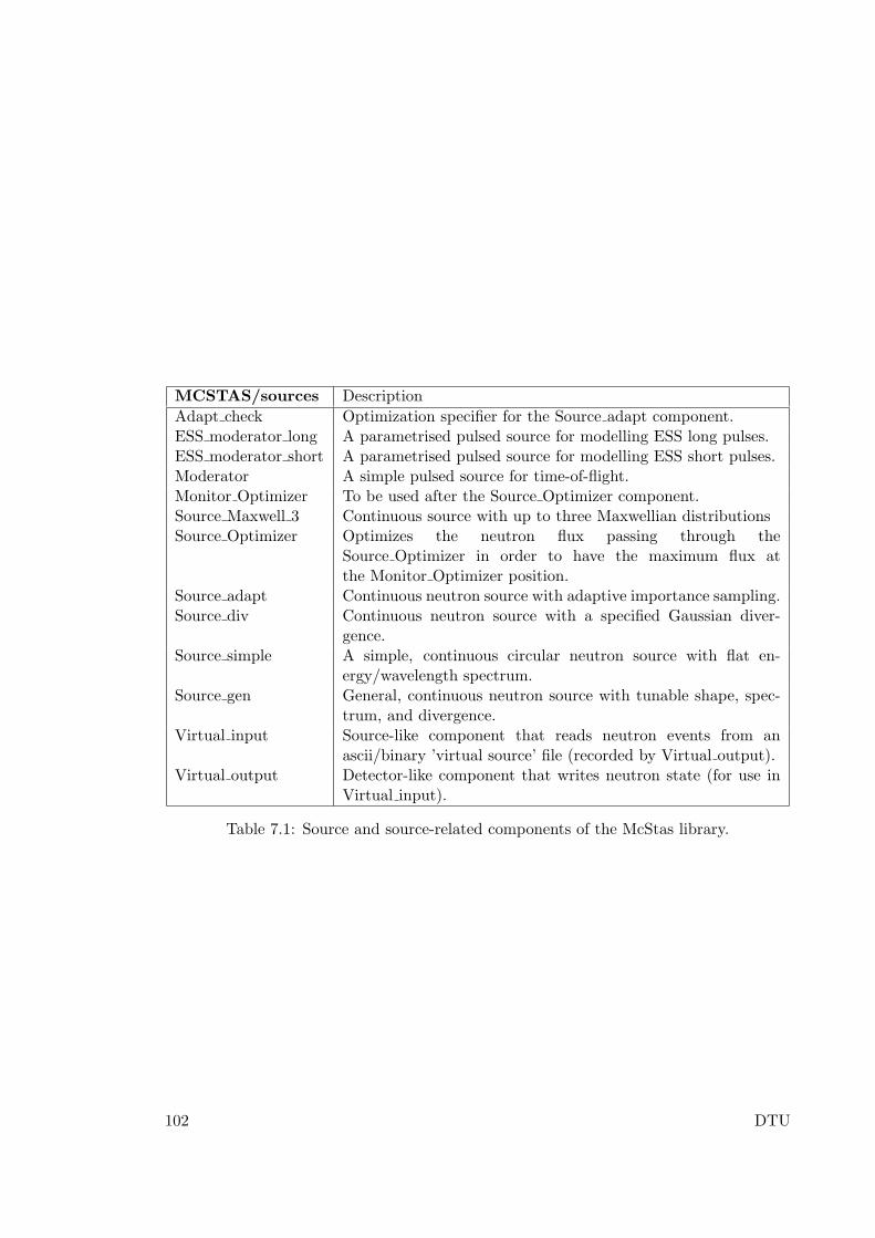
MCSTAS/sources Description

Adapt check Optimization specifier for the Source adapt component.ESS moderator long A parametrised pulsed source for modelling ESS long pulses.ESS moderator short A parametrised pulsed source for modelling ESS short pulses.Moderator A simple pulsed source for time-of-flight.Monitor Optimizer To be used after the Source Optimizer component.Source Maxwell 3 Continuous source with up to three Maxwellian distributionsSource Optimizer Optimizes the neutron flux passing through the

Source Optimizer in order to have the maximum flux atthe Monitor Optimizer position.

Source adapt Continuous neutron source with adaptive importance sampling.Source div Continuous neutron source with a specified Gaussian diver-

gence.Source simple A simple, continuous circular neutron source with flat en-

ergy/wavelength spectrum.Source gen General, continuous neutron source with tunable shape, spec-

trum, and divergence.Virtual input Source-like component that reads neutron events from an

ascii/binary ’virtual source’ file (recorded by Virtual output).Virtual output Detector-like component that writes neutron state (for use in

Virtual input).

Table 7.1: Source and source-related components of the McStas library.

102 DTU

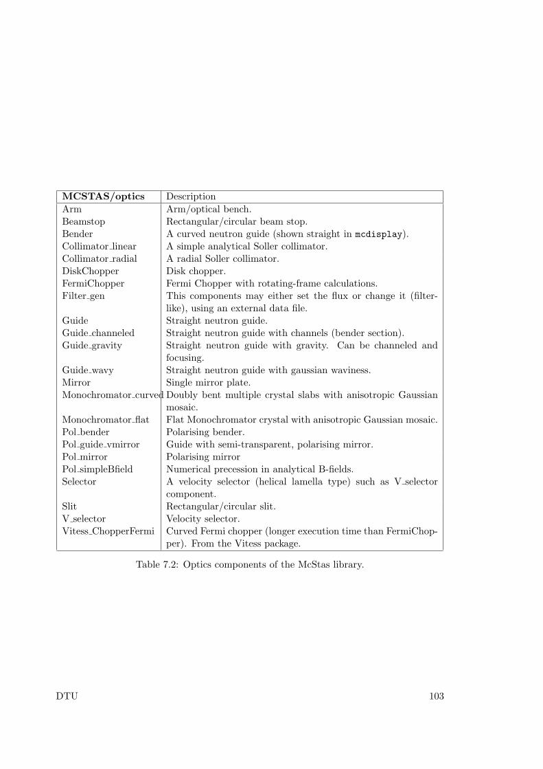
MCSTAS/optics Description

Arm Arm/optical bench.Beamstop Rectangular/circular beam stop.Bender A curved neutron guide (shown straight in mcdisplay).Collimator linear A simple analytical Soller collimator.Collimator radial A radial Soller collimator.DiskChopper Disk chopper.FermiChopper Fermi Chopper with rotating-frame calculations.Filter gen This components may either set the flux or change it (filter-

like), using an external data file.Guide Straight neutron guide.Guide channeled Straight neutron guide with channels (bender section).Guide gravity Straight neutron guide with gravity. Can be channeled and

focusing.Guide wavy Straight neutron guide with gaussian waviness.Mirror Single mirror plate.Monochromator curved Doubly bent multiple crystal slabs with anisotropic Gaussian

mosaic.Monochromator flat Flat Monochromator crystal with anisotropic Gaussian mosaic.Pol bender Polarising bender.Pol guide vmirror Guide with semi-transparent, polarising mirror.Pol mirror Polarising mirrorPol simpleBfield Numerical precession in analytical B-fields.Selector A velocity selector (helical lamella type) such as V selector

component.Slit Rectangular/circular slit.V selector Velocity selector.Vitess ChopperFermi Curved Fermi chopper (longer execution time than FermiChop-

per). From the Vitess package.

Table 7.2: Optics components of the McStas library.

DTU 103

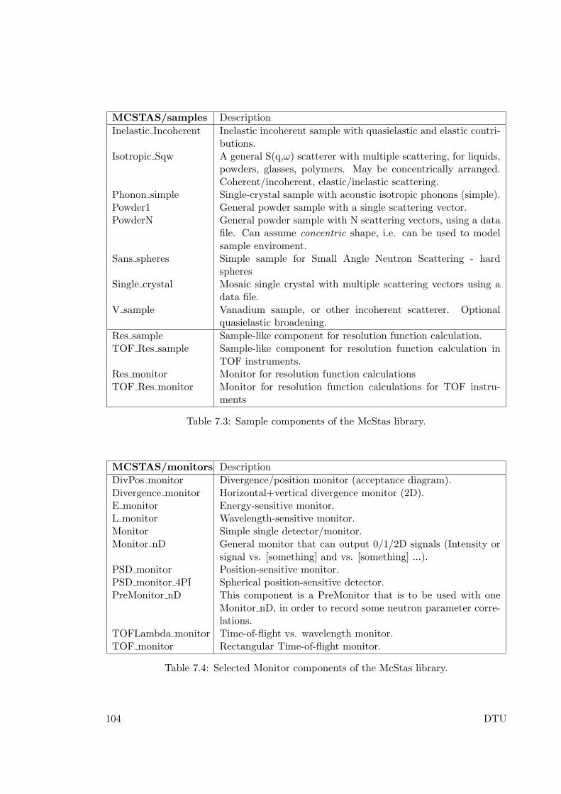
MCSTAS/samples Description

Inelastic Incoherent Inelastic incoherent sample with quasielastic and elastic contri-butions.

Isotropic Sqw A general S(q,ω) scatterer with multiple scattering, for liquids,powders, glasses, polymers. May be concentrically arranged.Coherent/incoherent, elastic/inelastic scattering.

Phonon simple Single-crystal sample with acoustic isotropic phonons (simple).Powder1 General powder sample with a single scattering vector.PowderN General powder sample with N scattering vectors, using a data

file. Can assume concentric shape, i.e. can be used to modelsample enviroment.

Sans spheres Simple sample for Small Angle Neutron Scattering - hardspheres

Single crystal Mosaic single crystal with multiple scattering vectors using adata file.

V sample Vanadium sample, or other incoherent scatterer. Optionalquasielastic broadening.

Res sample Sample-like component for resolution function calculation.TOF Res sample Sample-like component for resolution function calculation in

TOF instruments.Res monitor Monitor for resolution function calculationsTOF Res monitor Monitor for resolution function calculations for TOF instru-

ments

Table 7.3: Sample components of the McStas library.

MCSTAS/monitors Description

DivPos monitor Divergence/position monitor (acceptance diagram).Divergence monitor Horizontal+vertical divergence monitor (2D).E monitor Energy-sensitive monitor.L monitor Wavelength-sensitive monitor.Monitor Simple single detector/monitor.Monitor nD General monitor that can output 0/1/2D signals (Intensity or

signal vs. [something] and vs. [something] ...).PSD monitor Position-sensitive monitor.PSD monitor 4PI Spherical position-sensitive detector.PreMonitor nD This component is a PreMonitor that is to be used with one

Monitor nD, in order to record some neutron parameter corre-lations.

TOFLambda monitor Time-of-flight vs. wavelength monitor.TOF monitor Rectangular Time-of-flight monitor.

Table 7.4: Selected Monitor components of the McStas library.

104 DTU

MCSTAS/misc Description

Progress bar Displays status of a running simulation. May also trigger in-termediate SAVE.

Beam spy A monitor that displays mean statistics (no output file).Set pol sets polarisation vector.Vitess input Read neutron state parameters from a VITESS neutron file.Vitess output Write neutron state parameters to a VITESS neutron file.

Table 7.5: Miscellaneous components of the McStas library.

MCSTAS/contrib Description

Al window Aluminium transmission window.Collimator ROC Radial Oscillating Collimator (ROC).Exact radial coll Radial collimator.FermiChopper ILL Fermi Chopper with rotating frame and SM coating (straight).Filter graphite Pyrolytic graphite filter (analytical model).Filter powder Box-shaped powder filter based on Single crystal (unstable).Guide curved Non focusing continuous curved guide (shown curved).Guide honeycomb Neutron guide with gravity and honeycomb geometry. Can be

channeled and/or focusing.Guide tapering Rectangular tapered guide (parabolic, elliptic, sections ...).He3 cell Polarised 3He cell.ISIS moderator ISIS Target 1 and 2 moderator models based on MCNP calcu-

lations.Monochromator 2foc Doubly bent monochromator with multiple slabs.multi pipe a multi pipe slit (for SANS).PSD Detector Realistic detector model, with gas effects.PSD monitor rad A banana PSD monitor.SiC SiC multilayer sample for reflectivity simulations.SNS source SNS moderator models based on MCNP calculations.Source multi surfaces An array of sources described from spectrum tables.Virtual mcnp input Reads a PTRAC neutron events file from MCNP.Virtual mcnp output Writes a PTRAC neutron events file for MCNP.Virtual tripoli4 input Reads a ’Batch’ neutron events file from Tripoli 4.Virtual tripoli4 output Writes a ’Batch’ neutron events file for Tripoli 4.

Table 7.6: Contributed components of the McStas library.

DTU 105

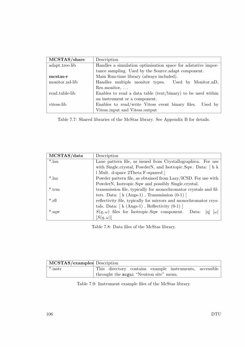
MCSTAS/share Description

adapt tree-lib Handles a simulation optimisation space for adatative impor-tance sampling. Used by the Source adapt component.

mcstas-r Main Run-time library (always included).monitor nd-lib Handles multiple monitor types. Used by Monitor nD,

Res monitor, . . .read table-lib Enables to read a data table (text/binary) to be used within

an instrument or a component.vitess-lib Enables to read/write Vitess event binary files. Used by

Vitess input and Vitess output

Table 7.7: Shared libraries of the McStas library. See Appendix B for details.

MCSTAS/data Description

*.lau Laue pattern file, as issued from Crystallographica. For usewith Single crystal, PowderN, and Isotropic Sqw. Data: [ h kl Mult. d-space 2Theta F-squared ]

*.laz Powder pattern file, as obtained from Lazy/ICSD. For use withPowderN, Isotropic Sqw and possibly Single crystal.

*.trm transmission file, typically for monochromator crystals and fil-ters. Data: [ k (Angs-1) , Transmission (0-1) ]

*.rfl reflectivity file, typically for mirrors and monochromator crys-tals. Data: [ k (Angs-1) , Reflectivity (0-1) ]

*.sqw S(q, ω) files for Isotropic Sqw component. Data: [q] [ω][S(q, ω)]

Table 7.8: Data files of the McStas library.

MCSTAS/examples Description

*.instr This directory contains example instruments, accessiblethrought the mcgui “Neutron site” menu.

Table 7.9: Instrument example files of the McStas library.

106 DTU

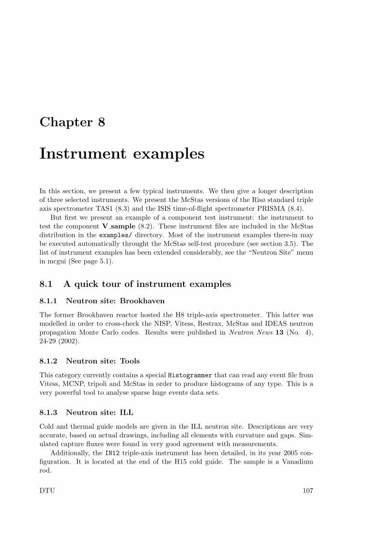
Chapter 8

Instrument examples

In this section, we present a few typical instruments. We then give a longer descriptionof three selected instruments. We present the McStas versions of the Risø standard tripleaxis spectrometer TAS1 (8.3) and the ISIS time-of-flight spectrometer PRISMA (8.4).

But first we present an example of a component test instrument: the instrument totest the component V sample (8.2). These instrument files are included in the McStasdistribution in the examples/ directory. Most of the instrument examples there-in maybe executed automatically throught the McStas self-test procedure (see section 3.5). Thelist of instrument examples has been extended considerably, see the “Neutron Site” menuin mcgui (See page 5.1).

8.1 A quick tour of instrument examples

8.1.1 Neutron site: Brookhaven

The former Brookhaven reactor hosted the H8 triple-axis spectrometer. This latter wasmodelled in order to cross-check the NISP, Vitess, Restrax, McStas and IDEAS neutronpropagation Monte Carlo codes. Results were published in Neutron News 13 (No. 4),24-29 (2002).

8.1.2 Neutron site: Tools

This category currently contains a special Histogrammer that can read any event file fromVitess, MCNP, tripoli and McStas in order to produce histograms of any type. This is avery powerful tool to analyse sparse huge events data sets.

8.1.3 Neutron site: ILL

Cold and thermal guide models are given in the ILL neutron site. Descriptions are veryaccurate, based on actual drawings, including all elements with curvature and gaps. Sim-ulated capture fluxes were found in very good agreement with measurements.

Additionally, the IN12 triple-axis instrument has been detailed, in its year 2005 con-figuration. It is located at the end of the H15 cold guide. The sample is a Vanadiumrod.

DTU 107

The IN6 instrument is a hybrid time-of-flight spectrometer with 3 monochromatorsand a Fermi chopper. The sample is an isotropic scatterer (liquid). It makes use of theSPLIT keyword to enhance statistics.

The ILL_TOF_Env example is a simple neutron pulse (e.g. from a chopper systemcoming out of IN4, IN5 or IN6) illuminating a sample, with a container around and acylinder shaped sample environment.

8.1.4 Neutron site: tests

This large set of examples shows simple instruments using particular components (samples,polarized beams, detectors). They may be used as starting point for further more complexmodels.

8.1.5 Neutron site: ISIS

You will find here examples of ISIS instruments, some of them using the ISIS moderatorcomponent (obtained from MCNP computations).

8.1.6 Neutron site: Risø

This section contains former Risø instruments, which constitue the default test series forthe McStas distribution.

8.1.7 Neutron site: PSI

The Focus time-of-flight instrument is, with the ILL IN6 and IN12 models, the mostadvanced example. It as been built from drawings, including the guide and all opticselements. Simulated capture fluxes were found in good agreement with measurements.

8.1.8 Neutron site: Tutorial

A typical diffractometer including a powder sample and a Rescal-type triple-axis modelsare in this category. Instrument parameters enable models to cope with most existinginstruments of these classes. The TAS model includes a basic in-plane UB-matrix trans-formation. It may be used to estimate the resolution functions of a TAS configuration.

8.1.9 Neutron site: ESS

This section contains design studies for the future, long-pulsed European Spallation Source(ESS). The only contents is currently the ESS_IN5_reprate instrument for simulating anIN5-TYPE (cold chopper) multi-frame spectrometer for the long-pulsed ESS. (Also servesas example instrument for Tunneling_sample.comp.)

8.2 A test instrument for the component V sample

This is one of many test instruments written with the purpose of testing the individualcomponents. We have picked this instrument both to present an example test instrumentand because it despite its simplicity has produced quite non-trivial results.

108 DTU

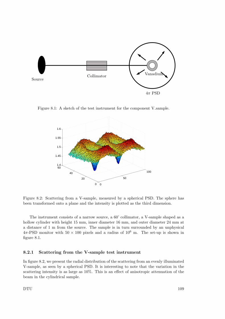
SourceCollimator

Vanadium

4π PSD

Figure 8.1: A sketch of the test instrument for the component V sample.

0

50

100

0

20

40

601.4

1.45

1.5

1.55

1.6

Figure 8.2: Scattering from a V-sample, measured by a spherical PSD. The sphere hasbeen transformed onto a plane and the intensity is plotted as the third dimension.

The instrument consists of a narrow source, a 60’ collimator, a V-sample shaped as ahollow cylinder with height 15 mm, inner diameter 16 mm, and outer diameter 24 mm ata distance of 1 m from the source. The sample is in turn surrounded by an unphysical4π-PSD monitor with 50 × 100 pixels and a radius of 106 m. The set-up is shown infigure 8.1.

8.2.1 Scattering from the V-sample test instrument

In figure 8.2, we present the radial distribution of the scattering from an evenly illuminatedV-sample, as seen by a spherical PSD. It is interesting to note that the variation in thescattering intensity is as large as 10%. This is an effect of anisotropic attenuation of thebeam in the cylindrical sample.

DTU 109

8.3 The triple axis spectrometer TAS1

With this instrument definition, we have tried to create a very detailed model of theconventional cold-source triple-axis spectrometer TAS1 at the now closed neutron sourceDR3 of Risø National Laboratory. Except for the cold source itself, all components usedhave quite realistic properties. Furthermore, the overall geometry of the instrument hasbeen adapted from the detailed technical drawings of the real spectrometer. The TAS 1simulation was the first detailed work performed with the McStas package. For furtherdetails see reference [48].

At the spectrometer, the channel from the cold source to the monochromator is asym-metric, since the first part of the channel is shared with other instruments. In the instru-ment definition, this is represented by three slits. For the cold source, we use a flat energydistribution (component Source flat) focusing on the third slit.

The real monochromator consist of seven blades, vertically focusing on the sample. Theangle of curvature is constant so that the focusing is perfect at 5.0 meV (20.0 meV for2nd order reflections) for a 1×1 cm2 sample. This is modeled directly in the instrumentdefinition using seven Monochromator components. The mosaicity of the pyrolyticgraphite crystals is nominally 30’ (FWHM) in both directions. However, the simulationsindicated that the horisontal mosaicities of both monochromator and analyser were morelikely 45’. This was used for all mosaicities in the final instrument definition.

The monochromator scattering angle, in effect determining the incoming neutron en-ergy, is for the real spectrometer fixed by four holes in the shielding, corresponding to theenergies 3.6, 5.0, 7.2, and 13.7 meV for first order neutrons. In the instrument definition,we have adapted the angle corresponding to 5.0 meV in order to test the simulationsagainst measurements performed on the spectrometer.

The width of the exit channel from the monochromator may be narrowed down frominitially 40 mm to 20 mm by an insert piece. In the simulations, we have chosen the 20 mmoption and modeled the channel with two slits to match the experimental set-up.

In the test experiments, we used two standard samples: An Al2O3 powder sample anda vanadium sample. The instrument definitions use either of these samples of the correctsize. Both samples are chosen to focus on the opening aperture of collimator 2 (the onebetween the sample and the analyser). Two slits, one before and one after the sample, arein the instrument definition set to the opening values which were used in the experiments.

The analyser of the spectrometer is flat and made from pyrolytic graphite. It is placedbetween an entry and an exit channel, the latter leading to a single detector. All this hasbeen copied into the instrument definition.

On the spectrometer, Soller collimators may be inserted at three positions: Betweenmonochromator and sample, between sample and analyser, and between analyser anddetector. In our instrument definition, we have used 30’, 28’, and 67’ collimators on thesethree positions, respectively.

An illustration of the TAS1 instrument is shown in figure 8.3. Test results and datafrom the real spectrometer are shown in Appendix 8.3.1.

110 DTU

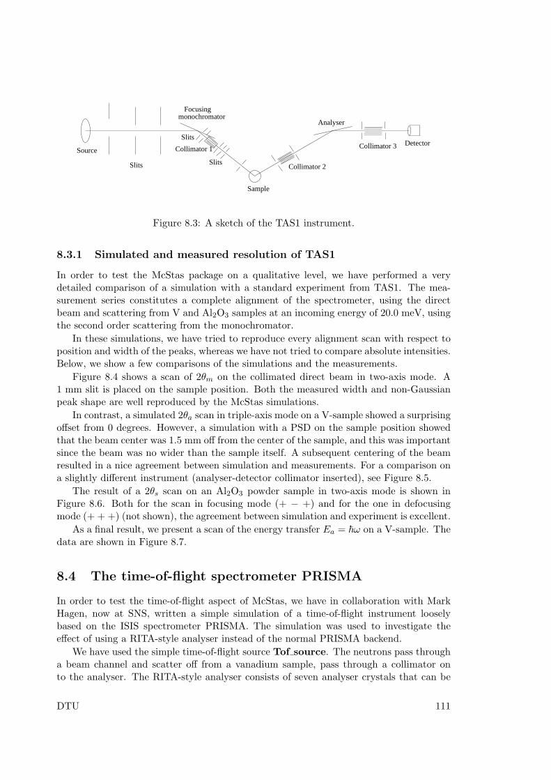
Source

Slits

Focusingmonochromator

Slits

Sample

Collimator 2

Analyser

Collimator 3 DetectorCollimator 1

Slits

Figure 8.3: A sketch of the TAS1 instrument.

8.3.1 Simulated and measured resolution of TAS1

In order to test the McStas package on a qualitative level, we have performed a verydetailed comparison of a simulation with a standard experiment from TAS1. The mea-surement series constitutes a complete alignment of the spectrometer, using the directbeam and scattering from V and Al2O3 samples at an incoming energy of 20.0 meV, usingthe second order scattering from the monochromator.

In these simulations, we have tried to reproduce every alignment scan with respect toposition and width of the peaks, whereas we have not tried to compare absolute intensities.Below, we show a few comparisons of the simulations and the measurements.

Figure 8.4 shows a scan of 2θm on the collimated direct beam in two-axis mode. A1 mm slit is placed on the sample position. Both the measured width and non-Gaussianpeak shape are well reproduced by the McStas simulations.

In contrast, a simulated 2θa scan in triple-axis mode on a V-sample showed a surprisingoffset from 0 degrees. However, a simulation with a PSD on the sample position showedthat the beam center was 1.5 mm off from the center of the sample, and this was importantsince the beam was no wider than the sample itself. A subsequent centering of the beamresulted in a nice agreement between simulation and measurements. For a comparison ona slightly different instrument (analyser-detector collimator inserted), see Figure 8.5.

The result of a 2θs scan on an Al2O3 powder sample in two-axis mode is shown inFigure 8.6. Both for the scan in focusing mode (+ − +) and for the one in defocusingmode (+ + +) (not shown), the agreement between simulation and experiment is excellent.

As a final result, we present a scan of the energy transfer Ea = ~ω on a V-sample. Thedata are shown in Figure 8.7.

8.4 The time-of-flight spectrometer PRISMA

In order to test the time-of-flight aspect of McStas, we have in collaboration with MarkHagen, now at SNS, written a simple simulation of a time-of-flight instrument looselybased on the ISIS spectrometer PRISMA. The simulation was used to investigate theeffect of using a RITA-style analyser instead of the normal PRISMA backend.

We have used the simple time-of-flight source Tof source. The neutrons pass througha beam channel and scatter off from a vanadium sample, pass through a collimator onto the analyser. The RITA-style analyser consists of seven analyser crystals that can be

DTU 111

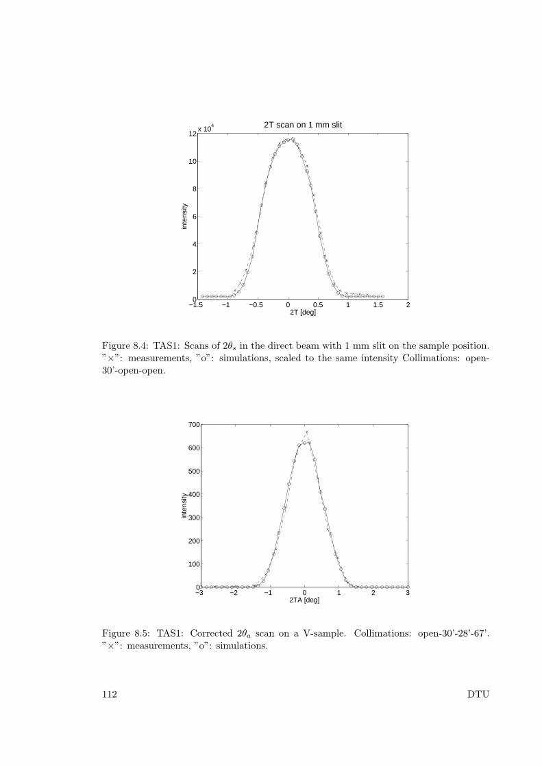
−1.5 −1 −0.5 0 0.5 1 1.5 20

2

4

6

8

10

12x 10

4

2T [deg]

inte

nsity

2T scan on 1 mm slit

Figure 8.4: TAS1: Scans of 2θs in the direct beam with 1 mm slit on the sample position.”×”: measurements, ”o”: simulations, scaled to the same intensity Collimations: open-30’-open-open.

−3 −2 −1 0 1 2 30

100

200

300

400

500

600

700

2TA [deg]

inte

nsity

Figure 8.5: TAS1: Corrected 2θa scan on a V-sample. Collimations: open-30’-28’-67’.”×”: measurements, ”o”: simulations.

112 DTU

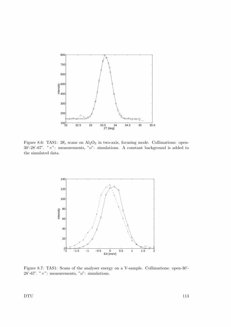
32 32.5 33 33.5 34 34.5 35 35.5100

200

300

400

500

600

700

800

2T [deg]

inte

nsity

Figure 8.6: TAS1: 2θs scans on Al2O3 in two-axis, focusing mode. Collimations: open-30’-28’-67’. ”×”: measurements, ”o”: simulations. A constant background is added tothe simulated data.

−2 −1.5 −1 −0.5 0 0.5 1 1.5 20

20

40

60

80

100

120

140

EA [meV]

inte

nsity

Figure 8.7: TAS1: Scans of the analyser energy on a V-sample. Collimations: open-30’-28’-67’. ”×”: measurements, ”o”: simulations.

DTU 113

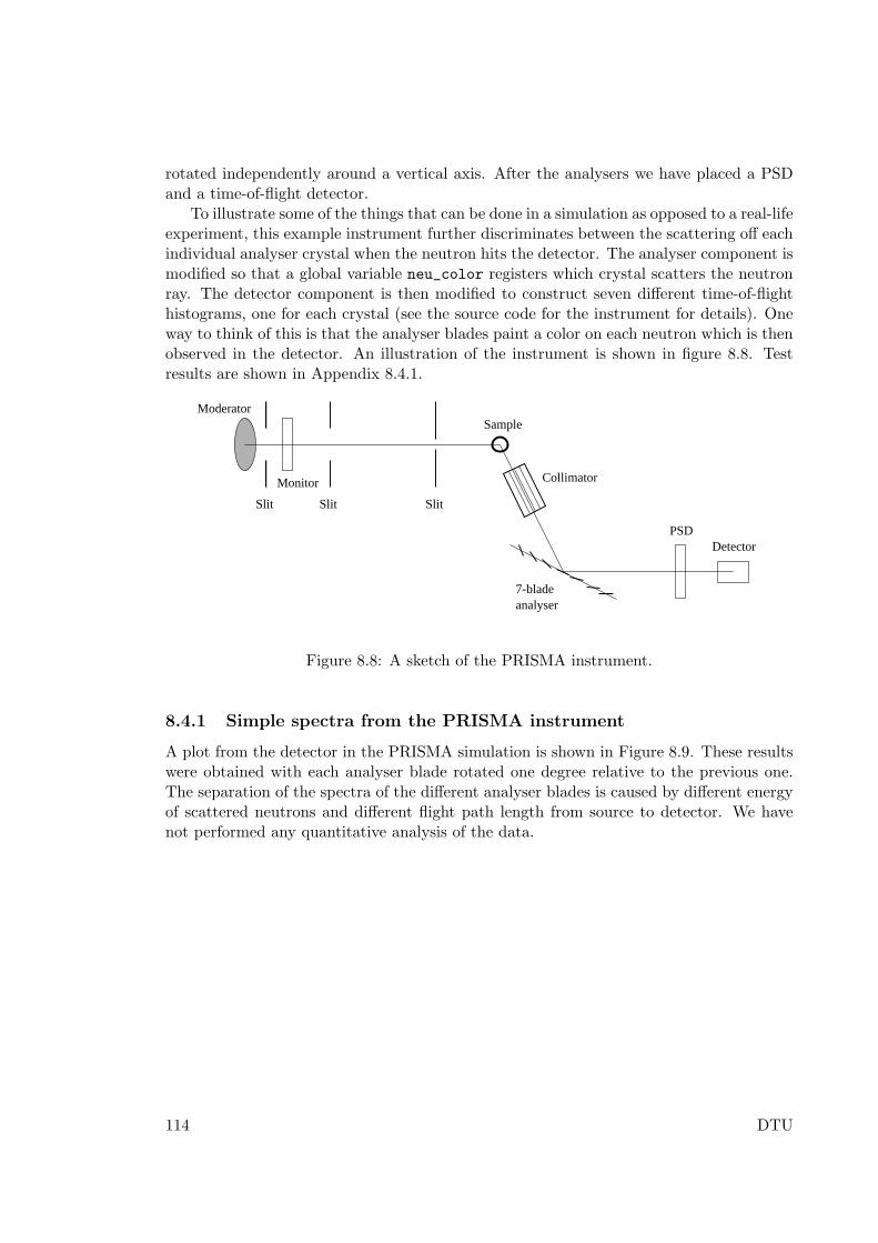
rotated independently around a vertical axis. After the analysers we have placed a PSDand a time-of-flight detector.

To illustrate some of the things that can be done in a simulation as opposed to a real-lifeexperiment, this example instrument further discriminates between the scattering off eachindividual analyser crystal when the neutron hits the detector. The analyser component ismodified so that a global variable neu_color registers which crystal scatters the neutronray. The detector component is then modified to construct seven different time-of-flighthistograms, one for each crystal (see the source code for the instrument for details). Oneway to think of this is that the analyser blades paint a color on each neutron which is thenobserved in the detector. An illustration of the instrument is shown in figure 8.8. Testresults are shown in Appendix 8.4.1.

7-bladeanalyser

Collimator

Moderator

Slit Slit

Monitor

Slit

Sample

PSDDetector

Figure 8.8: A sketch of the PRISMA instrument.

8.4.1 Simple spectra from the PRISMA instrument

A plot from the detector in the PRISMA simulation is shown in Figure 8.9. These resultswere obtained with each analyser blade rotated one degree relative to the previous one.The separation of the spectra of the different analyser blades is caused by different energyof scattered neutrons and different flight path length from source to detector. We havenot performed any quantitative analysis of the data.

114 DTU

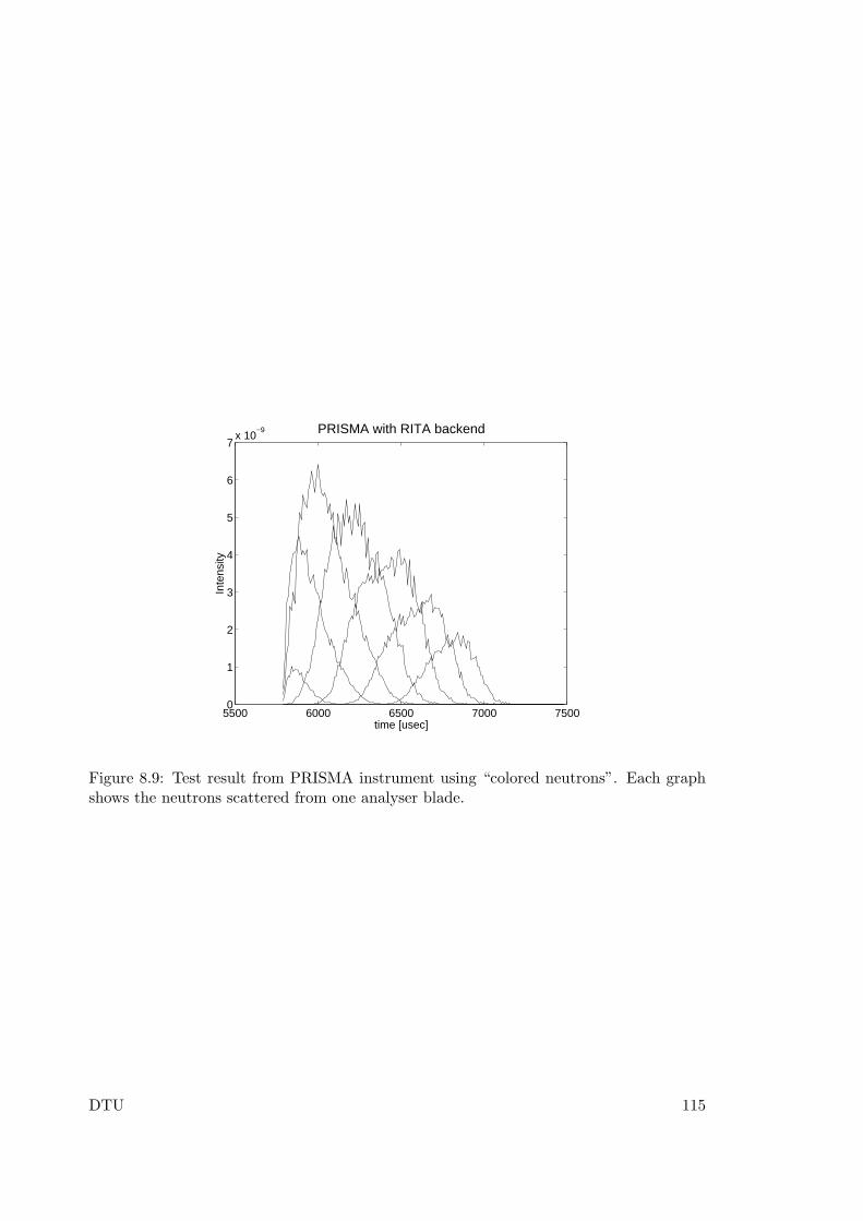
5500 6000 6500 7000 75000

1

2

3

4

5

6

7x 10

−9

time [usec]

Inte

nsity

PRISMA with RITA backend

Figure 8.9: Test result from PRISMA instrument using “colored neutrons”. Each graphshows the neutrons scattered from one analyser blade.

DTU 115

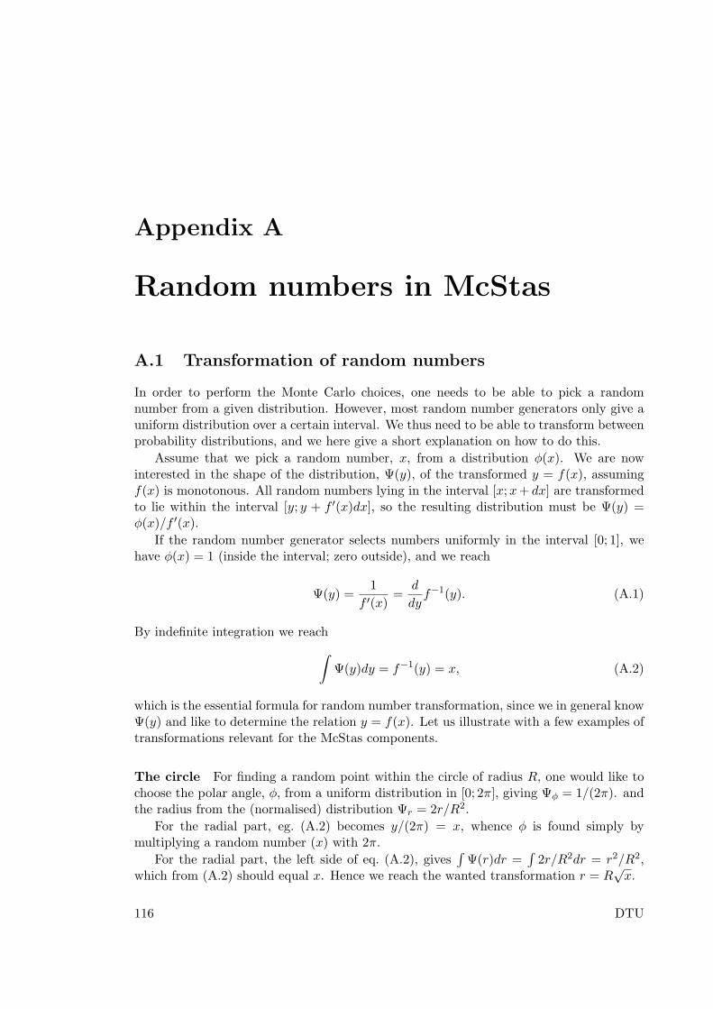
Appendix A

Random numbers in McStas

A.1 Transformation of random numbers

In order to perform the Monte Carlo choices, one needs to be able to pick a randomnumber from a given distribution. However, most random number generators only give auniform distribution over a certain interval. We thus need to be able to transform betweenprobability distributions, and we here give a short explanation on how to do this.

Assume that we pick a random number, x, from a distribution φ(x). We are nowinterested in the shape of the distribution, Ψ(y), of the transformed y = f(x), assumingf(x) is monotonous. All random numbers lying in the interval [x;x+ dx] are transformedto lie within the interval [y; y + f ′(x)dx], so the resulting distribution must be Ψ(y) =φ(x)/f ′(x).

If the random number generator selects numbers uniformly in the interval [0; 1], wehave φ(x) = 1 (inside the interval; zero outside), and we reach

Ψ(y) =1

f ′(x)=

d

dyf−1(y). (A.1)

By indefinite integration we reach

∫

Ψ(y)dy = f−1(y) = x, (A.2)

which is the essential formula for random number transformation, since we in general knowΨ(y) and like to determine the relation y = f(x). Let us illustrate with a few examples oftransformations relevant for the McStas components.

The circle For finding a random point within the circle of radius R, one would like tochoose the polar angle, φ, from a uniform distribution in [0; 2π], giving Ψφ = 1/(2π). andthe radius from the (normalised) distribution Ψr = 2r/R2.

For the radial part, eg. (A.2) becomes y/(2π) = x, whence φ is found simply bymultiplying a random number (x) with 2π.

For the radial part, the left side of eq. (A.2), gives∫

Ψ(r)dr =∫

2r/R2dr = r2/R2,which from (A.2) should equal x. Hence we reach the wanted transformation r = R

√x.

116 DTU

The sphere For finding a random point on the surface of the unit sphere, we need todetermine the two angles, (θ, φ).

Ψφ is chosen from a uniform distribution in [0; 2π], giving φ = 2πx as for the circle.The probability distribution of θ should be Ψθ = sin(θ) (for θ ∈ [0;π]), whence by

eq. (A.2) θ = cos−1(x).

Exponential decay In a simple time-of-flight source, the neutron flux decays expo-nentially after the initial activation at t = 0. We thus want to pick an initial neutronemission time from the normalised distribution Ψ(t) = exp(−t/τ)/τ . Use of Eq. (A.2)gives x = 1 − exp(−t/τ). For convenience we now use the random variable x1 = 1 − x(with the same distributions as x), giving the simple expression t = −τ ln(x1).

Normal distributions The important normal distribution can not be reached as asimple transformation of a uniform distribution. In stead, we rely on a specific algorithmfor selecting random numbers with this distribution.

A.2 Random generators

Even though there is the possibility to use the system random generator, as well as the ini-tial McStas version 1.1 random generator, the default algorithm is the so-called ”MersenneTwister”, by Makoto Matsumoto and Takuji Nishimura. Seehttp://www.math.sci.hiroshima-u.ac.jp/~m-mat/MT/emt.html for original source.

It is considered today to be by far the best random generator, which means that bothits period is extremely large 219937−1, and cross-correlations are negligible, i.e distributionsare homogeneous and independent up to 623 dimensions. It is also extremely fast.

DTU 117

Appendix B

Libraries and constants

The McStas Library contains a number of built-in functions and conversion constantswhich are useful when constructing components. These are stored in the share directoryof the MCSTAS library.

Within these functions, the ’Run-time’ part is available for all component/instrumentdescriptions. The other parts are dynamic, that is they are not pre-loaded, but onlyimported once when a component requests it using the %include McStas keyword. Forinstance, within a component C code block, (usually SHARE or DECLARE):

%include "read_table-lib"

will include the ’read table-lib.h’ file, and the ’read table-lib.c’ (unless the --no-runtimeoption is used with mcstas). Similarly,

%include "read_table-lib.h"

will only include the ’read table-lib.h’. The library embedding is done only once for allcomponents (like the SHARE section). For an example of implementation, seeRes monitor.

In this Appendix, we present a short list of both each of the library contents and therun-time features.

B.1 Run-time calls and functions (mcstas-r)

Here we list a number of preprogrammed macros which may ease the task of writingcomponent and instrument definitions.

B.1.1 Neutron propagation

Propagation routines perform all necessary operations to transport neutron rays fromone point to an other. Except when using the special ALLOW_BACKPROP; call prior toexectuting any PROP_* propagation, the neutron rays which have negative propagationtimes are removed automatically.

• ABSORB. This macro issues an order to the overall McStas simulator to interruptthe simulation of the current neutron history and to start a new one.

118 DTU

• PROP Z0. Propagates the neutron to the z = 0 plane, by adjusting (x, y, z) and taccordingly from knowledge of the neutron velocity (vx, vy, vz). If the propagationtime is negative, the neutron ray is absorbed, except if a ALLOW_BACKPROP; preceedsit.

For components that are centered along the z-axis, use the _intersect functions todetermine intersection time(s), and then a PROP_DT call.

• PROP DT(dt). Propagates the neutron through the time interval dt, adjusting(x, y, z) and t accordingly from knowledge of the neutron velocity. This macro auto-matically calls PROP GRAV DT when the --gravitation option has been set forthe whole simulation.

• PROP GRAV DT(dt, Ax,Ay,Az). Like PROP DT, but it also includes gravityusing the acceleration (Ax,Ay,Az). In addition to adjusting (x, y, z) and t, also(vx, vy, vz) is modified.

• ALLOW BACKPROP. Indicates that the next propagation routine will not re-move the neutron ray, even if negative propagation times are found. Further propa-gations are not affected.

• SCATTER. This macro is used to denote a scattering event inside a component.It should be used e.g to indicate that a component has interacted with the neutronray (e.g. scattered or detected). This does not affect the simulation (see, however,Beamstop), and it is mainly used by the MCDISPLAY section and the GROUP modifierSee also the SCATTERED variable (below).

B.1.2 Coordinate and component variable retrieval

• MC GETPAR(comp, outpar). This may be used in e.g. the FINALLY section ofan instrument definition to reference the output parameters of a component.

• NAME CURRENT COMP gives the name of the current component as a string.

• POS A CURRENT COMP gives the absolute position of the current compo-nent. A component of the vector is referred to as POS A CURRENT COMP.i wherei is x, y or z.

• ROT A CURRENT COMP and ROT R CURRENT COMP give the ori-entation of the current component as rotation matrices (absolute orientation andthe orientation relative to the previous component, respectively). A component of arotation matrix is referred to as ROT A CURRENT COMP[m][n], where m and nare 0, 1, or 2 standing for x, y and z coordinates respectively.

• POS A COMP(comp) gives the absolute position of the component with the namecomp. Note that comp is not given as a string. A component of the vector is referredto as POS A COMP(comp).i where i is x, y or z.

• ROT A COMP(comp) and ROT R COMP(comp) give the orientation of thecomponent comp as rotation matrices (absolute orientation and the orientation rela-tive to its previous component, respectively). Note that comp is not given as a string.

DTU 119

A component of a rotation matrice is referred to as ROT A COMP(comp)[m][n],where m and n are 0, 1, or 2.

• INDEX CURRENT COMP is the number (index) of the current component(starting from 1).

• POS A COMP INDEX(index) is the absolute position of component index.POS A COMP INDEX (INDEX CURRENT COMP) is the same asPOS A CURRENT COMP. You may usePOS A COMP INDEX (INDEX CURRENT COMP+1)to make, for instance, your component access the position of the next component(this is usefull for automatic targeting). A component of the vector is referred to asPOS A COMP INDEX(index).i where i is x, y or z.

• POS R COMP INDEX works the same as above, but with relative coordinates.

• STORE NEUTRON(index, x, y, z, vx, vy, vz, t, sx, sy, sz, p) stores the current neu-tron state in the trace-history table, in local coordinate system. index is usually IN-DEX CURRENT COMP. This is automatically done when entering each componentof an instrument.

• RESTORE NEUTRON(index, x, y, z, vx, vy, vz, t, sx, sy, sz, p) restores the neu-tron state to the one at the input of the component index. To ignore a componenteffect, use RESTORE NEUTRON (INDEX CURRENT COMP,x, y, z, vx, vy, vz, t, sx, sy, sz, p) at the end of its TRACE section, or in its EXTENDsection. These neutron states are in the local component coordinate systems.

• SCATTERED is a variable set to 0 when entering a component, which is incre-mented each time a SCATTER event occurs. This may be used in the EXTEND

sections to determine whether the component interacted with the current neutronray.

• extend list(n, &arr, &len, elemsize). Given an array arr with len elements each ofsize elemsize, make sure that the array is big enough to hold at least n elements, byextending arr and len if necessary. Typically used when reading a list of numbersfrom a data file when the length of the file is not known in advance.

• mcset ncount(n). Sets the number of neutron histories to simulate to n.

• mcget ncount(). Returns the number of neutron histories to simulate (usually setby option -n).

• mcget run num(). Returns the number of neutron histories that have been simu-lated until now.

B.1.3 Coordinate transformations

• coords set(x, y, z) returns a Coord structure (like POS A CURRENT COMP) withx, y and z members.

120 DTU

• coords get(P, &x, &y, &z) copies the x, y and z members of the Coord structureP into x, y, z variables.

• coords add(a, b), coords sub(a, b), coords neg(a) enable to operate on coordi-nates, and return the resulting Coord structure.

• rot set rotation(Rotation t, φx, φy, φz) Get transformation matrix for rotation firstφx around x axis, then φy around y, and last φz around z. t should be a ’Rotation’([3][3] ’double’ matrix).

• rot mul(Rotation t1, Rotation t2, Rotation t3) performs t3 = t1.t2.

• rot copy(Rotation dest, Rotation src) performs dest = src for Rotation arrays.

• rot transpose(Rotation src, Rotation dest) performs dest = srct.

• rot apply(Rotation t, Coords a) returns a Coord structure which is t.a

B.1.4 Mathematical routines

• NORM(x, y, z). Normalizes the vector (x, y, z) to have length 1.

• scalar prod(ax, ay, az, bx, by, bz). Returns the scalar product of the two vectors(ax, ay, az) and (bx, by, bz).

• vec prod(&ax,&ay,&az,bx,by,bz, cx,cy,cz). Sets (ax, ay, az) equal to the vector prod-uct (bx, by, bz)× (cx, cy, cz).

• rotate(&x,&y,&z,vx,vy,vz,ϕ,ax,ay,az). Set (x, y, z) to the result of rotating thevector (vx, vy, vz) the angle ϕ (in radians) around the vector (ax, ay, az).

• normal vec(&nx, &ny, &nz, x, y, z). Computes a unit vector (nx, ny, nz) normalto the vector (x, y, z).

• solve 2nd order(*t, A, B, C). Solves the 2nd order equation At2 + Bt + C = 0and returns the smallest positive solution into pointer *t.

B.1.5 Output from detectors

Details about using these functions are given in the McStas User Manual.

• DETECTOR OUT 0D(...). Used to output the results from a single detector.The name of the detector is output together with the simulated intensity and es-timated statistical error. The output is produced in a format that can be read byMcStas front-end programs.

• DETECTOR OUT 1D(...). Used to output the results from a one-dimensionaldetector. Integrated intensities error etc. is also reported as for DETECTOR OUT 0D.

• DETECTOR OUT 2D(...). Used to output the results from a two-dimentionaldetector. Integrated intensities error etc. is also reported as for DETECTOR OUT 0D.

DTU 121

• DETECTOR OUT 3D(...). Used to output the results from a three-dimentionaldetector. Arguments are the same as in DETECTOR OUT 2D, but with an addi-tional z axis. Resulting data files are treated as 2D data, but the 3rd dimension isspecified in the type field. Integrated intensities error etc. is also reported as forDETECTOR OUT 0D.

• mcinfo simulation(FILE *f, mcformat, char *pre, char *name) is used to appendthe simulation parameters into file f (see for instance Res monitor). Internalvariable mcformat should be used as specified. Please contact the authors forfurther information.

B.1.6 Ray-geometry intersections

• inside rectangle(&x, &y, x, xw, yh). Return 1 if −xw/2 ≤ x ≤ xw/2 AND−yh/2 ≤ y ≤ yh/2. Else return 0.

• box intersect(&t1, &t2, x, y, z, vx, vy, vz, dx, dy, dz). Calculates the (0, 1, or2) intersections between the neutron path and a box of dimensions dx, dy, and dz,centered at the origin for a neutron with the parameters (x, y, z, vx, vy, vz). Thetimes of intersection are returned in the variables t1 and t2, with t1 < t2. In thecase of less than two intersections, t1 (and possibly t2) are set to zero. The functionreturns true if the neutron intersects the box, false otherwise.

• cylinder intersect(&t1, &t2, x, y, z, vx, vy, vz, r, h). Similar to box intersect,but using a cylinder of height h and radius r, centered at the origin.

• sphere intersect(&t1, &t2, x, y, z, vx, vy, vz, r). Similar to box intersect, butusing a sphere of radius r.

B.1.7 Random numbers

• rand01(). Returns a random number distributed uniformly between 0 and 1.

• randnorm(). Returns a random number from a normal distribution centered around0 and with σ = 1. The algorithm used to sample the normal distribution is explainedin Ref. [49, ch.7].

• randpm1(). Returns a random number distributed uniformly between -1 and 1.

• randtriangle(). Returns a random number from a triangular distribution between-1 and 1.

• randvec target circle(&vx, &vy, &vz, &dΩ, aimx, aimy, aimz, rf ). Generates arandom vector (vx, vy, vz), of the same length as (aimx, aimy, aimz), which is targetedat a disk centered at (aimx, aimy, aimz) with radius rf (in meters), and perpendicularto the aim vector.. All directions that intersect the circle are chosen with equalprobability. The solid angle of the circle as seen from the position of the neutron isreturned in dΩ. This routine was previously called randvec target sphere (whichstill works).

122 DTU

• randvec target rect angular(&vx, &vy, &vz, &dΩ, aimx, aimy, aimz,h,w,Rot)does the same as randvec target circle but targetting at a rectangle with angu-lar dimensions h and w (in radians, not in degrees as other angles). The rota-tion matrix Rot is the coordinate system orientation in the absolute frame, usuallyROT A CURRENT COMP.

• randvec target rect(&vx, &vy, &vz, &dΩ, aimx, aimy, aimz,height, width,Rot) isthe same as randvec target rect angular but height and width dimensions are givenin meters. This function is useful to e.g. target at a guide entry window or analyzerblade.

B.2 Reading a data file into a vector/matrix (Table input,read table-lib)

The read_table-lib provides functionalities for reading text (and binary) data files. Touse this library, add a %include "read_table-lib" in your component definition DE-CLARE or SHARE section. Tables are structures of type t_Table (see read_table-lib.hfile for details):

/* t_Table structure (most important members) */

double *data; /* Use Table_Index(Table, i j) to extract [i,j] element */

long rows; /* number of rows */

long columns; /* number of columns */

char *header; /* the header with comments */

char *filename; /* file name or title */

double min_x; /* minimum value of 1st column/vector */

double max_x; /* maximum value of 1st column/vector */

Available functions to read a single vector/matrix are:

• Table Init(&Table, rows, columns) returns an allocated Table structure. Userows = columns = 0 not to allocate memory and return an empty table. Callsto Table Init are optional, since initialization is being performed by other functionsalready.

• Table Read(&Table, filename, block) reads numerical block number block (0 toconcatenate all) data from text file filename into Table, which is as well initializedin the process. The block number changes when the numerical data changes its size,or a comment is encoutered (lines starting by ’# ; % /’). If the data could not beread, then Table.data is NULL and Table.rows = 0. You may then try to read itusing Table Read Offset Binary. Return value is the number of elements read.

• Table Read Offset(&Table, filename, block, &offset, nrows) does the same asTable Read except that it starts at offset offset (0 means begining of file) and readsnrows lines (0 for all). The offset is returned as the final offset reached after readingthe nrows lines.

DTU 123

• Table Read Offset Binary(&Table, filename, type, block, &offset, nrows, ncolumns)does the same as Table Read Offset, but also specifies the type of the file (may be”float” or ”double”), the number nrows of rows to read, each of them having ncolumns

elements. No text header should be present in the file.

• Table Rebin(&Table) rebins all Table rows with increasing, evenly spaced firstcolumn (index 0), e.g. before using Table Value. Linear interpolation is performedfor all other columns. The number of bins for the rebinned table is determined fromthe smallest first column step.

• Table Info(Table) print information about the table Table.

• Table Index(Table,m, n) reads the Table[m][n] element.

• Table Value(Table, x, n) looks for the closest x value in the first column (index 0),and extracts in this row the n-th element (starting from 0). The first column is thusthe ’x’ axis for the data.

• Table Free(&Table) free allocated memory blocks.

• Table Value2d(Table, X, Y ) Uses 2D linear interpolation on a Table, from (X,Y)coordinates and returns the corresponding value.

Available functions to read an array of vectors/matrices in a text file are:

• Table Read Array(File, &n) read and split file into as many blocks as necessaryand return a t_Table array. Each block contains a single vector/matrix. This onlyworks for text files. The number of blocks is put into n.

• Table Free Array(&Table) free the Table array.

• Table Info Array(&Table) display information about all data blocks.

The format of text files is free. Lines starting by ’# ; % /’ characters are consideredto be comments, and stored in Table.header. Data blocks are vectors and matrices. Blocknumbers are counted starting from 1, and changing when a comment is found, or thecolumn number changes. For instance, the file ’MCSTAS/data/BeO.trm’ (Transmissionof a Berylium filter) looks like:

# BeO transmission, as measured on IN12

# Thickness: 0.05 [m]

# [ k(Angs-1) Transmission (0-1) ]

# wavevector multiply

1.0500 0.74441

1.0750 0.76727

1.1000 0.80680

...

Binary files should be of type ”float” (i.e. REAL*32) and ”double” (i.e. REAL*64), andshould not contain text header lines. These files are platform dependent (little or bigendian).

124 DTU

The filename is first searched into the current directory (and all user additional loca-tions specified using the -I option, see the ’Running McStas ’ chapter in the User Manual),and if not found, in the data sub-directory of the MCSTAS library location. This way, youdo not need to have local copies of the McStas Library Data files (see table 7.8).

A usage example for this library part may be:

t_Table Table; // declare a t_Table structure

char file[]="BeO.trm"; // a file name

double x,y;

Table_Read(&Table, file, 1); // initialize and read the first numerical block

Table_Info(Table); // display table informations

...

x = Table_Index(Table, 2,5); // read the 3rd row, 6th column element

// of the table. Indexes start at zero in C.

y = Table_Value(Table, 1.45,1); // look for value 1.45 in 1st column (x axis)

// and extract 2nd column value of that row

Table_Free(&Table); // free allocated memory for table

Additionally, if the block number (3rd) argument of Table Read is 0, all blocks will beconcatenated. The Table Value function assumes that the ’x’ axis is the first column(index 0). Other functions are used the same way with a few additional parameters, e.g.specifying an offset for reading files, or reading binary data.

This other example for text files shows how to read many data blocks:

t_Table *Table; // declare a t_Table structure array

long n;

double y;

Table = Table_Read_Array("file.dat", &n); // initialize and read the all numerical block

n = Table_Info_Array(Table); // display informations for all blocks (also returns n)

y = Table_Index(Table[0], 2,5); // read in 1st block the 3rd row, 6th column element

// ONLY use Table[i] with i < n !

Table_Free_Array(Table); // free allocated memory for Table

You may look into, for instance, the source files for Monochromator curved orVirtual input for other implementation examples.

B.3 Monitor nD Library

This library gathers a few functions used by a set of monitors e.g. Monitor nD, Res monitor,Virtual output, etc. It may monitor any kind of data, create the data files, and may dis-play many geometries (for mcdisplay). Refer to these components for implementationexamples, and ask the authors for more details.

DTU 125

B.4 Adaptive importance sampling Library

This library is currently only used by the components Source adapt and Adapt check.It performs adaptive importance sampling of neutrons for simulation efficiency optimiza-tion. Refer to these components for implementation examples, and ask the authors formore details.

B.5 Vitess import/export Library

This library is used by the components Vitess input and Vitess output, as well as themcstas2vitess utility. Refer to these components for implementation examples, and askthe authors for more details.

B.6 Constants for unit conversion etc.

The following predefined constants are useful for conversion between units

Name Value Conversion from Conversion to

DEG2RAD 2π/360 Degrees RadiansRAD2DEG 360/(2π) Radians DegreesMIN2RAD 2π/(360 · 60) Minutes of arc RadiansRAD2MIN (360 · 60)/(2π) Radians Minutes of arcV2K 1010 ·mN/~ Velocity (m/s) k-vector (A−1)K2V 10−10 · ~/mN k-vector (A−1) Velocity (m/s)VS2E mN/(2e) Velocity squared (m2 s−2) Neutron energy (meV)

SE2V√

2e/mN Square root of neutron en-ergy (meV1/2)

Velocity (m/s)

FWHM2RMS 1/√

8 log(2) Full width half maximum Root mean square(standard deviation)

RMS2FWHM√

8 log(2) Root mean square (stan-dard deviation)

Full width half maxi-mum

MNEUTRON 1.67492 · 10−27 kg Neutron mass, mn

HBAR 1.05459 · 10−34 Js Planck constant, ~PI 3.14159265... πFLT MAX 3.40282347E+38F a big float value

126 DTU

Appendix C

The McStas terminology

This is a short explanation of phrases and terms which have a specific meaning withinMcStas. We have tried to keep the list as short as possible with the risk that the readermay occasionally miss an explanation. In this case, you are more than welcome to contactthe McStas core team.

• Arm A generic McStas component which defines a frame of reference for othercomponents.

• Component One unit (e.g. optical element) in a neutron spectrometer. These areconsidered as Types of elements to be instantiated in an Instrument description.

• Component Instance A named Component (of a given Type) inserted in an In-strument description.

• Definition parameter An input parameter for a component. For example theradius of a sample component or the divergence of a collimator.

• Input parameter For a component, either a definition parameter or a settingparameter. These parameters are supplied by the user to define the characteristics ofthe particular instance of the component definition. For an instrument, a parameterthat can be changed at simulation run-time.

• Instrument An assembly of McStas components defining a neutron spectrometer.

• Kernel The McStas language definition and the associated compiler

• McStas Monte Carlo Simulation of Triple Axis Spectrometers (the name of thispackage). Pronounciation ranges from mex-tas, to mac-stas and m-c-stas.

• Output parameter An output parameter for a component. For example the countsin a monitor. An output parameter may be accessed from the instrument in whichthe component is used using MC_GETPAR.

• Run-time C code, contained in the files mcstas-r.c and mcstas-r.h included inthe McStas distribution, that declare functions and variables used by the generatedsimulations.

DTU 127

• Setting parameter Similar to a definition parameter, but with the restriction thatthe value of the parameter must be a number.

128 DTU

Bibliography

[1] K. Lefmann and K. Nielsen. Neutron News, 10, 20–23, 1999.

[2] See http://www.mcstas.org.

[3] See http://trac.mccode.org/report.

[4] See http://ts-2.isis.rl.ac.uk/.

[5] See http://www.ess-europe.de.

[6] See http://neutron-eu.net/en/.

[7] See http://mcnsi.risoe.dk/.

[8] See http://strider.lansce.lanl.gov/NISP/Welcome.html.

[9] P. A. Seeger, L. L. Daemen, T. G. Thelliez, and R. P. Hjelm. Physica B, 283, 433,2000.

[10] J. Saroun and J. Kulda. Physica B, 234, 1102, 1997. See websitehttp://omega.ujf.cas.cz/restrax/.

[11] P. Willendrup, E. Farhi, and K. Lefmann. Physica B, 350, 735, 2004.

[12] D. Wechsler, G. Zsigmond, F. Streffer, and F. Mezei. Neutron News, 25, 11, 2000.

[13] See http://www.hmi.de/projects/ess/vitess/.

[14] W.-T. Lee and X.-L. Wang. Neutron News, 13, 30, 2002. See websitehttp://www.sns.gov/ideas/.

[15] See http://neutrons-dev.ornl.gov/eqsans/software/ib/.

[16] http://code.google.com/p/jnads/.

[17] J.R.D. Copley. J. Neut. Research, 1, 21, 1993.

[18] E. Farhi, T. Hansen, A. Wildes, R. Ghosh, and K. Lefmann. Appl. Phys., A 74,S1471, 2002.

[19] C. Schanzer, P. Boni, U. Filges, and T. Hils. Nucl. Instr. Meth., A 529, 63, 2004.

DTU 129

[20] G. Zsigmond, K. Lieutenant, and S. Manoshin et al. Nucl. Instr. Meth., A 529, 218,2004.

[21] K. Lieutenant. J. Phys.: Condens. Matter, 17, S167, 2005.

[22] T. E. Mason, K. N. Clausen, G. Aeppli, D. F. McMorrow, and J. K. Kjems. Can. J.Phys., 73, 697–702, 1995.

[23] K. N. Clausen, D. F. McMorrow, K. Lefmann, G. Aeppli, T. E. Mason, A. Schroder,M. Issikii, M. Nohara, and H. Takagi. Physica B, 241-243, 50–55, 1998.

[24] K. Lefmann, D. F. McMorrow, H. M. Rønnow, K. Nielsen, K. N. Clausen, B. Lake,and G. Aeppli. Physica B, 283, 343–354, 2000.

[25] See http://www.sns.gov/.

[26] H. Maier-Leibnitz and T. Springer. Reactor Sci. Technol., 17, 217, 1963.

[27] D.F.R. Mildner. Nucl. Instr. Meth., A290, 189, 1990.

[28] R.A. Lowde. J. Nucl. Energy, Part A: Reactor Sci., 11, 69, 1960.

[29] J.R.D. Copley. Nucl. Instr. Meth., A510, 318, 2003.

[30] E. Fermi, J. Marshall, and L. Marshall. Phys. Rev., 72, 193, 1947.

[31] J. Peters. Nucl. Instr. Meth., A540, 419, 2005.

[32] C.D. Clark, E.W.J. Mitchell, D.W. Palmer, and I.H. Wilson. J. Sci. Instrum., 43, 1,1966.

[33] A.K. Freund. Nucl. Instr. Meth., 213, 495, 1983.

[34] V.F. Sears. Acta Cryst., A53, 35, 1997.

[35] G. Shirane, S.M. Shapiro, and J.M. Tranquada. Neutron Scattering with a Triple-AxisSpectrometer. Cambridge University Press, 2002.

[36] L. Alianelli. J. Appl. Cryst., 37, 732, 2004.

[37] V. Radeka. IEEE Trans. Nucl. Sci., NS-21, 51, 1974.

[38] V. Peskov, G. Charpak, W. Dominik, and F. Sauli. Nucl. Instr. and Meth., A277,547, 1989.

[39] G. Manzin, B. Guerard, F.A.F. Fraga, and L.M.S. Margato. Nucl. Instr. Meth.,A535, 102, 2004.

[40] L. D. Cussen. J. Appl. Cryst., 36, 1204, 2003.

[41] F. James. Rep. Prog. Phys., 43, 1145, 1980.

[42] J. R. D. Copley, P. Verkerk, A. A. van Well, and H. Fredrikze. Comput. Phys.Commun., 40, 337, 1986.

130 DTU

[43] D.F.R. Mildner, C.A. Pellizari, and J.M. Carpenter. Acta. Cryst. A, 33, 954, 1977.

[44] Grimmett, G. R., and Stirzakerand D. R. Probability and Random Processes, 2ndEdition. Clarendon Press, Oxford, 1992.

[45] J.A. Nelder and R. Mead. Computer Journal, 7, 308–313, 1965.

[46] W.H. Press, S.A. Teukolsky, W.T. Vetterling, and B.P. Flannery. Numerical Recipes(2nd Edition). Cambridge University Press, 2002.

[47] See http://www.neutron.anl.gov/nexus/.

[48] A. Abrahamsen, N. B. Christensen, and E. Lauridsen. McStas simulations of the TAS1spectrometer. Student’s report, Niels Bohr Institute, University of Copenhagen, 1998.

[49] W. H. Press, S. A. Teukolsky, W. T. Vetterling, and B. P. Flannery. NumericalRecipes in C. Cambridge University Press, 1986.

DTU 131

Index

Bugs, 12, 58, 66, 73, 81, 83

Can not compile, 69, 72, 96Code generation options, 33Comments, 69Components, 13, 73Coordinate system, 68

Data formats, 37, 40, 46, 57–60, 72, 88Customization, 90

Embedded C code, 69, 72, 78Environment variable

MCSTAS, 33MCSTAS FORMAT, 52PGPLOT DEV, 45, 53

Environment variableBROWSER, 56, 98EDITOR, 45MCSTAS, 98, 115, 122MCSTAS CC, 16MCSTAS CFLAGS, 16MCSTAS FORMAT, 16, 30, 37, 54, 58PGPLOT DEV, 54PGPLOT DIR, 45, 53, 54

Gravitation, 68Grid computing, 57Grid computing, 47, 61

Installing, 14, 16, 52Instruments, 71, 77ITERATE, 82

Kernel, 12, 67Keyword, 69

%include, 33, 69, 78, 115ABSOLUTE, 74AT, 74COMPONENT, 73

COPY, 79, 95

DECLARE, 72, 86

DEFINE

COMPONENT, 84

INSTRUMENT, 71

DEFINITION PARAMETERS, 84

END, 75, 92

EXTEND, 78, 95, 116

FINALLY, 75, 91

GROUP, 78, 79, 116

INITIALIZE, 72, 87

ITERATE, 82

JUMP, 82

MCDISPLAY, 91, 116

NEXUS, 72

OUTPUT PARAMETERS, 85, 86

POLARISATION PARAMETERS, 85

PREVIOUS, 74

RELATIVE, 74

ROTATED, 74

SAVE, 75, 88

SETTING PARAMETERS, 84

SHARE, 87, 115

SPLIT, 83

STATE PARAMETERS, 85

TRACE, 73, 87

WHEN, 81, 82

Library, 115

adapt tree-lib, 123

Components, 13, 33, 56, 74, 98

contrib, 98, 102

data, 103, 122

misc, 102

monitors, 101

obsolete, 98

optics, 100

samples, 101

132 DTU

share, 67, 69, 103, 115sources, 99

Instruments, 103mcstas-r, see Library/Run-timemonitor nd-lib, 122read table-lib (Read Table), 69, 120Run-time, 12, 34, 67, 69, 103, 115ABSORB, 87, 115ALLOW BACKPROP, 88, 115DETECTOR CUSTOM HEADER, 90DETECTOR OUT, 88MC GETPAR, 86, 116NAME CURRENT COMP, 116POS A COMP, 116POS A CURRENT COMP, 116PROP DT, 115PROP GRAV DT, 115PROP Z0, 87, 115RESTORE NEUTRON, 116ROT A COMP, 116ROT A CURRENT COMP, 116SCATTER, 79, 88, 115SCATTERED, 79, 116STORE NEUTRON, 116

Shared, see Library/Components/sharevitess-lib, 56, 123

MCNP, 37, 40mcstas-hosts, 61Monte Carlo method, 22, 113

Accuracy, 26Adaptive sampling, 25Direction focusing, 25Random number, Mersenne Twister, 114Stratified sampling, 25

MPI, 45, 47, 61MYSELF, 82

Neutron state and units, 68NEXT, 82

Optimization, 35, 41

Parallel computing, 61Parameters

Definition, 73, 84Instruments, 36, 50, 71

Optimization, 42, 50Optional, default value, 36, 71, 85Protecting, see Keyword/OUTPUTScans, 50Setting, 73, 84

PREVIOUS, 82

Removed neutron events, 75, 88, 116ROTATED, 82

Signal handler, 38INT signal, 75TERM signal, 75USR2 signal, 75

Simulation optimization, 35

Testing the distribution, 16Tools, 14, 28

HDF, 60, 72HTML, 37, 60IDL, 38, 57, 59Matlab, 30, 37, 52, 53, 55, 57, 59mcconvert, 57mcdisplay, 52mcdoc, 56, 96, 98mcformat, 57, 61mcgui, 29, 32, 45, 52, 54mcplot, 30, 38, 46, 48, 51, 54, 58mcresplot, 55mcrun, 32, 50mcstas2vitess, 56, 123NeXus, 45, 60, 72Octave, 57Perl libraries, 45, 53, 54, 56PGPLOT, 30, 37, 45, 52–55, 58Scilab, 30, 37, 38, 52, 53, 55, 57, 59VRML, 60VRML/OpenGL, 37, 38, 52, 57

Tripoli, 37, 40

Vitess, 37, 40, 56

DTU 133

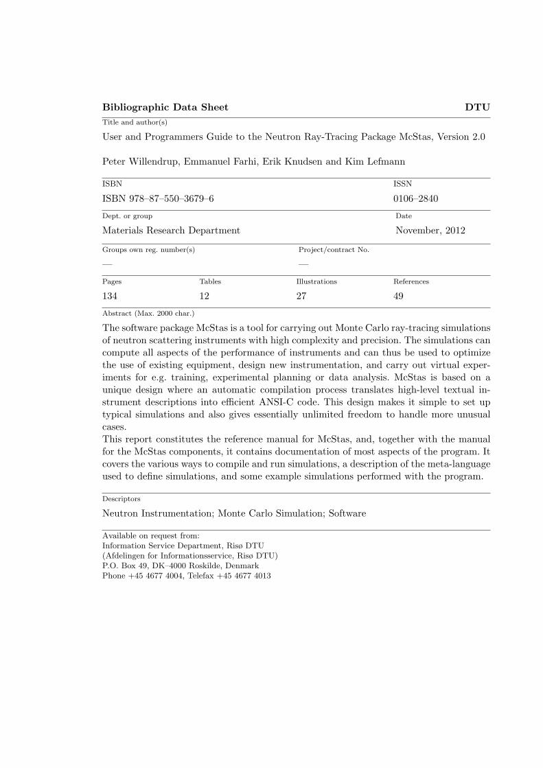
Bibliographic Data Sheet DTU

Title and author(s)

User and Programmers Guide to the Neutron Ray-Tracing Package McStas, Version 2.0

Peter Willendrup, Emmanuel Farhi, Erik Knudsen and Kim Lefmann

ISBN

ISBN 978–87–550–3679–6

ISSN

0106–2840

Dept. or group

Materials Research Department

Date

November, 2012

Groups own reg. number(s)

—

Project/contract No.

—

Pages

134

Tables

12

Illustrations

27

References

49

Abstract (Max. 2000 char.)

The software package McStas is a tool for carrying out Monte Carlo ray-tracing simulationsof neutron scattering instruments with high complexity and precision. The simulations cancompute all aspects of the performance of instruments and can thus be used to optimizethe use of existing equipment, design new instrumentation, and carry out virtual exper-iments for e.g. training, experimental planning or data analysis. McStas is based on aunique design where an automatic compilation process translates high-level textual in-strument descriptions into efficient ANSI-C code. This design makes it simple to set uptypical simulations and also gives essentially unlimited freedom to handle more unusualcases.This report constitutes the reference manual for McStas, and, together with the manualfor the McStas components, it contains documentation of most aspects of the program. Itcovers the various ways to compile and run simulations, a description of the meta-languageused to define simulations, and some example simulations performed with the program.

Descriptors

Neutron Instrumentation; Monte Carlo Simulation; Software

Available on request from:Information Service Department, Risø DTU(Afdelingen for Informationsservice, Risø DTU)P.O. Box 49, DK–4000 Roskilde, DenmarkPhone +45 4677 4004, Telefax +45 4677 4013

PhysicsDepartment, TechnicalUniversityofDenmark ... · PhysicsDepartment,...

Documents

Transcript of PhysicsDepartment, TechnicalUniversityofDenmark ... · PhysicsDepartment,...