PhysicsMaple provides a state-of-the-art environment for algebraic computations in Physics, with emphasis on ensuring that the computational experience is as natural as possible. The theme of the Physics project for Maple 2017 has been the consolidation of the functionalityintroduced in previous releases, together with significant enhancements and new functionality in General Relativity, in connection with classification of solutions to Einstein'sequations and tensor representations to work in the embedded 3D curved space, relevant in numerical relativity, and Field Theory, in connection with computational representations for the objects entering the Standard Model in particle physics.

Taking all together, there are more than 300 enhancements throughout the entire packageincreasing robustness, versatility and functionality, extending once more the range of Physics-related algebraic computations that can be done using computer algebra software and in a natural way.

As part of its commitment to providing the best possible environment for algebraic computations in Physics, Maplesoft launched a Maple Physics: Research and Development web site with Maple 18, which enabled users to download research versions, ask questions, and provide feedback. The results from this accelerated exchange with people around the world have been incorporated into the Physics package in Maple 2017.

General Relativity: classification of solutions to Einstein's equations and the Tetrads packageIn Maple 2016, the digitizing of the database of solutions to Einstein's equations was finished, added to the standard Maple library, with all the metrics from "Stephani, H.; Kramer, D.; MacCallum, M.; Hoenselaers, C.; and Herlt, E., Exact Solutions to Einstein's Field Equations". These metrics can be loaded to work with them, or change them, or searched using g_ (the Physics command representing the spacetime metric that also sets the metric to your choice in one go) or using the command DifferentialGeometry:-Library:-MetricSearch.

Related to these developments, in Maple 2017, the Physics:-Tetrads package has been vastly improved and extended, now including new commands like PetrovType and SegreType to classify these metrics, and the TransformTetrad now has an optioncanonicalform to automatically derive a transformation and put the tetrad in canonical form (reorientation of the axis of the local system of references), a

(1)(1)

> >

relevant step in resolving the equivalence between two metrics.

In the PDEtools package, you have the mathematical tools - including a complete symmetry approach - to work with the underlying partial differential equations. By combining the functionality of the Physics:-Tetrads package, the Physics:-TransformCoordinates command, and the ability to compute Riemann invariants and Weyl scalars, you can also formulate and, depending on the metrics also resolve, the equivalence problem; that is: to answer whether or not, given two metrics, they can be obtained from each other by a transformation of coordinates, as well as compute the transformation.

Depending on the context, or textbook, two different signatures are used in the

Physics and in Landau's Course for Theoretical Physics, the main reference for the Maple Physics project. Two other computational representations of those same signatures are , with time in position 4; for the computer, this difference in representation is relevant since it indicates the computational position where the component 0 is to be found (either 1 or 4). This difference also changes the position of the time coordinate in the ordered list of the coordinates. Changing the signature to follow a textbook or just for convenience thus entails redefining the metric rearranging lines and columns in its matrix representation and/or changing the sign, and reordering the coordinates, operations prone to mistakes. To handle these redefinitions of the metric and coordinates according to a change in the signature, a new command Redefine (options fromsignature,tosignature), got added to the Physics package.

Examples

Petrov and Segre types, tetrads in canonical form

Setting lowercaselatin letters to represent tetrad indices

There are six Petrov types: I, II, III, D, N and O. Start with a spacetime metric of Petrov type "I" (the numbers always refer to the equation number in the "Exact solutions to Einstein's field equations" textbook)

> >

(2)(2)

> >

(6)(6)

> >

(4)(4)

(3)(3)

(5)(5)> >

(7)(7)> >

> >

Resetting the signature of spacetime from "- - - C" to `- C C C` in order to match the signature in the database of metrics:

The Weyl scalars are derived from the Weyl tensor and the null vectors of the Newman-Penrose formalism (l_, n_, m_ and mb_)

For presentation simplicity, without absolute values, assume that x is positive or 0and recompute the Weyl scalars

Relevant in connection with the equivalence problem between two metrics, the Petrov type of this metric is

"I"

> >

(2)(2)

> >

(11)(11)

(12)(12)

(8)(8)

(10)(10)

(9)(9)

> >

(13)(13)

> >

> >

> >

> >

and the Plebanski-Segre type is

Two spacetime metrics with different classification cannot be different coordinate representations of the same metric (if the classification is the same the question is still undecided). The same computation but tracking the principal roots behind this classification

"I"

The principal polynomial only, having four different roots corresponding to Petrov type "I"

An example of Petrov type III and a canonical form for the corresponding tetrad.

For presentation simplicity, assume that z and the parameter are positive

The Petrov and Plebanski-Segre types, the default tetrad and the corresponding Weyl scalars:

> >

(2)(2)

(14)(14)

(15)(15)

(16)(16)

> >

> >

(19)(19)

> >

(17)(17)

> >

> >

(18)(18)

> >

> >

"III"

These scalars are not in canonical form. Compute then a canonical form for this tetrad (i.e. rotate the tetrad such that the Weyl scalars match the canonical form shown in the Petrov classification table) and set this rotated tetrad (using Setup), then recompute the Weyl scalars

The scalars now match the requirement for canonical form shown in the Petrov classification table for type III. In this example, the canonical form computed for the tetrad

(2)(2)

(14)(14)> >

(20)(20)

(19)(19)

> >

> >

is not much more complicated than the default tetrad (16) that is not in canonical form, but depending on the example the canonical form can be significantly more complicated.

Examples of transforming the tetrad into canonical form for spacetimes of Petrov types II, N and D can be seen by performing the same steps above departing fromthe metrics of the database with numbers g_[[24, 37, 7]], g_[[12, 6, 1]] and g_[[12, 8, 4]].

Together with the developments above, the TransformTetrad got thoroughly reviewed and its transformation functionality extended in order to perform the six traditional rotations that leave different null vectors of the Newman-Penrose formalism unchanged in direction or length,

Load the Schwarzschild metric in spherical coordinates; you can input g_[Schwarzschild] or the simpler

An orthonormal tetrad (this is the one used by default) is

(2)(2)

(14)(14)

(24)(24)

> >

(22)(22)

(21)(21)

(23)(23)

> >

> >

(19)(19)

> >

> >

> >

Type of tetrad: orthonormal true

The key observation here is that the orientation of the axis of the local system of references (the tetrad system) is arbitrary and with them the values of the Weyl scalars too. So, you can perform a Lorentz transformation on the tetrad, without changing the spacetime metric g_ or its Petrov classification while fixing the values of the Weyl scalars in one of the possible forms (classes) shown in thePetrov classification table.

The transformations that you can perform with TransformTetrad are either the standard ones, of classes I, II or III specified in the description of TransformTetrad, or arbitrary. For example, transform the orthonormal tetrad above using a null rotation with fixed l_, where l_ and the related NULL vectors of the Newman-Penrose formalism (commands of the Tetrads package) satisfy

> >

(2)(2)

(27)(27)

(14)(14)

> >

(24)(24)

> >

(28)(28)

(21)(21)

> >

(19)(19)

(26)(26)

> >

> >

(25)(25)

(29)(29)

> >

> >

Note the transformation parameter E introduced by TransformTetrad. You can replace it by a value or assign it, or you may want to Assume that this parameter is, for instance, real

Now is this a tetrad? Of what type?

Type of tetrad: null true

TransformTetrad applies a transformation on a tetrad but does not set the value of e_ to this result. For that purpose, i.e. to effectively rotate the tetrad system of references to match the orientation/tetrad you want, use Setup. Following this reorientation of the tetrad, all the components of tensors in the local (tetrad) system of references, as for instance gamma_, lambda_ and the tetrad components of spacetime tensors, automatically change. For example, the Ricci rotation coefficients gamma_ follow this change of value of the components of

according to their definition

So before setting (26) as the new tetrad, for comparison purposes below, track firstthe value of the Ricci rotation coefficient with covariant indices 1, 2, 1

> >

(2)(2)

(14)(14)

(32)(32)

(24)(24)

(21)(21)

> >

> >

(19)(19)

> >

> >

(29)(29)

(30)(30)

> >

> >

(31)(31)

Set now (26) as the new tetrad

The new value of

Equivalence for Schwarzschild metric (spherical and Kruskal coordinates)

Formulation of the problem (remove mixed coordinates)

Setting lowercaselatin letters to represent tetrad indices

* Partial match of 'auto' against keyword 'automaticsimplification'

The departure point, Schwarzschild metric in spherical coordinates

(35)(35)

(2)(2)

(33)(33)

(34)(34)

(14)(14)

(24)(24)

(36)(36)

(21)(21)

> >

> >

> >

(19)(19)

> >

> >

(29)(29)

> >

> >

> >

Introduce now Kruskal coordinates following the literature (see Wikipedia) and the corresponding line element involving "mixed" coordinates

The mixing of variables is visible: in the line element above is in Kruskal coordinates but you also see r , which belongs to the X (not K) coordinates.

For the purpose of formulating problem free of this mixing of coordinates, set the metric now to be (35)

(38)(38)

(2)(2)

> >

(33)(33)

(14)(14)

(24)(24)

(36)(36)

(40)(40)

(21)(21)

> >

(37)(37)

> >

(19)(19)

(41)(41)

> >

> >

> >

> >

> >

(29)(29)

(39)(39)

> >

To remove the mix of coordinates, introduce a transformation with unknown transformation functions , change variables, and resolve for the transformation functions (this in itself is resolving a form of equivalence problem).

Equate to (33) and solve

> >

(44)(44)

(2)(2)

(33)(33)

(14)(14)

(24)(24)

(36)(36)

(21)(21)

(45)(45)

> >

> >

> >

(19)(19)

(41)(41)

> >

> >

(42)(42)

(29)(29)

> >

(43)(43)

> >

Without loss of generality, set

Check it out:

Compute the inverse of the transformation (42)

This inverse transformation involves the LambertW function. Set now the metric to be the standard Schwarzschild's metric in spherical coordinates (33) and use itr to get he form of the metric entirely in Kruskal coordinates

(2)(2)

(33)(33)

(14)(14)

(24)(24)

(36)(36)

(21)(21)

> >

> >

(19)(19)

(41)(41)

> >

> >

> >

(29)(29)

(47)(47)

> >

(46)(46)

So this is Schwarzschild's solution all in Kruskal coordinates

This metric involves the LambertW function in a non-simplifiable form.

Solving the Equivalence

We now have the two forms: (44) in spherical and (47) in Kruskal coordinates, sowe can formulate the equivalence problem from one coordinate system to the other one.

The transformation to be resolved does not need to involve because neither nor enter either of the two metrics.

> >

(2)(2)

(33)(33)

(14)(14)

(24)(24)

(36)(36)

(21)(21)

> >

> >

> >

> >

(19)(19)

(41)(41)

(50)(50)

> >

(49)(49)

> >

(29)(29)

> >

(46)(46)

(48)(48)

The transformation does not need to involve or because they enter the metrics in exactly the same position and with the same dependence.

In addition the Weyl scalars of both metrics are in canonical form and the only scalar different from zero, that is does not depend on any of )

So we look for a generic transformation from spherical to Kruskal of the form

The metric set in this moment is in spherical coordinates, (46), so change using (48) and equate to (47) in Kruskal coordinates

> >

(2)(2)

(33)(33)

(24)(24)

(36)(36)

(54)(54)

(21)(21)

(19)(19)

(50)(50)

> >

(29)(29)

> >

(52)(52)

(14)(14)

> >

> >

> >

(41)(41)

> >

(53)(53)

(51)(51)

> >

> >

(46)(46)

This is a nonlinear, non-rational PDE system in two unknowns depending on two independent variables (see (48)). You can now either call pdsolve on (50), solving the problem in one step, or first split into cases without solving any differential equation, just doing differential elimination, to see the cases

By using differential elimination we removed all nonlinearities, the problem is actually easy for the differential equation routines

So the transformation of coordinates resolving the equivalence between (44) and (47) is

Check this result transforming (44) fully written in spherical coordinates into (47) fully written in Kruskal coordinates

(57)(57)

(2)(2)

(33)(33)

(24)(24)

(36)(36)

(54)(54)

(21)(21)

(19)(19)

(50)(50)

(55)(55)

> >

> >

(29)(29)

> >

> >

(14)(14)> >

> >

(41)(41)

(56)(56)

> >

> >

> >

(46)(46)

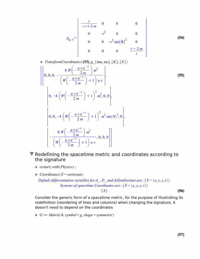
Redefining the spacetime metric and coordinates according to the signature

Consider the generic form of a spacetime metric, for the purpose of illustrating its redefinition (reordering of lines and columns) when changing the signature, it doesn't need to depend on the coordinates

(57)(57)

(2)(2)

(33)(33)

(24)(24)

(36)(36)

(54)(54)

> >

(21)(21)

> >

(19)(19)

(50)(50)

(29)(29)

> >

(14)(14)

> >

(61)(61)

(60)(60)

> >

> >

(58)(58)

(41)(41)

> >

(59)(59)

> >

> >

(62)(62)

> >

(46)(46)

Set the metric, and in the same call check the value of signature: it is (- - - +)

Track the line element

Change now the signature by reversing the position of the time-like component, from 4 to 1

Neither the metric nor the coordinates change: t is still in position 4 and the component (1, 1) of the metric is still

This design gives you freedom to set things as necessary. However, after changing the signature we may also want to redefine the coordinates - place t in position 1 - and possibly also the metric reordering its lines and rows accordingly. A new command for that purpose is , to which you need to indicate the previous signature (or a new signature, to explore the effect of a change before

(64)(64)

(57)(57)

(2)(2)

(33)(33)

> >

(24)(24)

(36)(36)

(54)(54)

(21)(21)

> >

(63)(63)

(19)(19)

(50)(50)

> >

(67)(67)

(29)(29)

> >

> >

(14)(14)

(68)(68)

(66)(66)

> >

> >

(41)(41)

> >

> >

> >

> >

(46)(46)

(65)(65)

doing it) and an indication of whether you want to redefine the metric, the coordinates or all:

These redefinitions however were not set, the keywords coordinates, metric, or all only trigger the change, t is still in position 4 and the component (1,1) of the metric is still

You can now either use the output of this routine to redefine things using the Setup command, or do all in one go using any of the keywords setcoordinates, setmetric, or setall, for example

Now t in position 1 and the component (1,1) of the metric equal to

> >

(57)(57)

(2)(2)

(33)(33)

(70)(70)

(24)(24)

(36)(36)

(54)(54)

(21)(21)

(71)(71)

(19)(19)

(50)(50)

(29)(29)

> >

> >

(14)(14)

(68)(68)

(69)(69)

(72)(72)

> >

> >

> >

> >

(41)(41)

> >

> >

(73)(73)

> >

(46)(46)

Note that, despite the reordering of lines and columns in the metric, because we also reordered the variables, the line element has not changed:

0

This routine is particularly useful when working with metrics from the database of solutions to Einstein's equations, all of which reset the signature to (-+++) when loaded. For example:

Resetting the signature of spacetime from "C - - -" to `- C C C` in order to match the signature in the database of metrics:

Note above the message about resetting the signature; query about:

(57)(57)

(2)(2)

(33)(33)

(24)(24)

(36)(36)

(54)(54)

(21)(21)

(19)(19)

(50)(50)

> >

(29)(29)

(14)(14)

(68)(68)

> >

> >

(41)(41)

> >

> >

> >

(74)(74)

> >

(73)(73)

> >

(46)(46)

(75)(75)

How would this metric and coordinates look with the original signature (---+) ?

By entering the command above replacing all by setall not only the list of coordinates and metric matrix form are returned but they are also set in one go.

The 3D metric and the ThreePlusOne (3 + 1) new Physics subpackageIn the general theory of relativity, can be any quantities defining the position of bodies in space and the time coordinate can be defined by an arbitrarily running clock. In order to define simultaneity (synchronizing clocks located at different points in space) as well as determine actual space distances and time intervals in terms of these quantities , it is relevant to split the spacetime mathematical description of gravity into its space and time parts. For this purpose, three new commands were added to the Physics package:

Decompose, to decompose 4D tensorial expressions (free and/or contracted indices) into the space and time parts.

gamma_, representing the three-dimensional metric tensor, with which the elementof spatial distance is defined as

Redefine, to redefine the coordinates and the spacetime metric according to changes in the signature from any of the four possible signatures ,

, and ( to any of the other ones.

Examples

Define now an arbitrary tensor A

(57)(57)

(81)(81)

(2)(2)

(33)(33)

(24)(24)

(36)(36)

(54)(54)

> >

(78)(78)

(21)(21)

(19)(19)

(50)(50)

> >

> >

(82)(82)

(79)(79)

(29)(29)

> >

> >

(76)(76)

> >

(14)(14)

(68)(68)

> >

(80)(80)

> >

> >

(41)(41)

(77)(77)

> >

> >

(73)(73)

> >

(46)(46)

Defined objects with tensor properties

So A is a 4D tensor with only one free index, where the position of the time-like component is the position of the different sign in the signature, that you can query about via

To perform a decomposition into space and time, set - for instance - the lowercase latin letters from i to s to represent spaceindices and

Accordingly, the 3+1 decomposition of A is

The 3+1 decomposition of the inert representation %g_[mu,nu] of the 4D spacetime metric; use the inert representation when you do not want the actual components of the metric appearing in the output

Note the position of the component %g_[0, 0], related to the trailing position of the time-like component in the signature .

Compare the decomposition of the 4D inert with the decomposition of the 4D active spacetime metric

(57)(57)

(2)(2)

(89)(89)

(33)(33)

(24)(24)

(36)(36)

(54)(54)

> >

(86)(86)

(83)(83)

(21)(21)

(87)(87)

(19)(19)

(50)(50)

(84)(84)

> >

(29)(29)

> >

> >

(76)(76)

(14)(14)

> >

(68)(68)

> >

> >

(88)(88)

(85)(85)

> >

> >

(41)(41)

> >

> >

> >

(73)(73)

> >

(46)(46)

Note that in general the 3D space part of is not equal to the 3D metric whose

definition includes another term (see [1] Landau & Lifshitz, eq.(84.7)).

The 3D space part of is actually equal to the 3D metric

To derive the formula (83) for the covariant components of the 3D metric,Decompose into 3+1 the identity

To the side, for illustration purposes, these are the 3 + 1 decompositions, first excluding the repeated indices, then excluding the free indices

Compare with a full decomposition

Eq is a symmetric matrix of equations involving non-contracted occurrences of g , g and g . Isolate, in Eq , g , that you input as %g_[~j, ~0], and substitute intoEq

(57)(57)

(2)(2)

(33)(33)

(24)(24)

(36)(36)

(54)(54)

(21)(21)

(90)(90)

(19)(19)

(50)(50)

> >

> >

> >

(29)(29)

> >

> >

(92)(92)

(76)(76)

(14)(14)

(68)(68)

> >

> >

(93)(93)

(41)(41)

(91)(91)

> >

> >

(73)(73)

> >

(46)(46)

Collect g , that you input as %g_[~j, ~i]

Since the right-hand side is the identity matrix and, from (84), , the expression between parenthesis, multiplied by -1, is the reciprocal of the

contravariant 3D metric , that is the covariant 3D metric , in accordance to its

definition for the signature

References[1] Landau, L.D., and Lifshitz, E.M. The Classical Theory of Fields, Course of Theoretical Physics Volume 2, fourth revised English edition. Elsevier, 1975.

A description is also key in the study of gravitational waves, black holes, neutron stars and in general to study the evolution of physical system in general relativity by running numerical simulations as traditional initial value (Cauchy) problems. In this framework, Maple 2017 introduces a new package ThreePlusOne , to case Einstein's equations in a 3+1 form, that is, representing spacetime as a stack of nonintersecting 3-hypersurfaces (not necessarily actual space) with:

Computational representations for the spatial metric that is induced by on the

3-dimensional hypersurfaces, and the related covariant derivative, Christoffel symbols and Ricci and Riemann tensors.

Computational representations for the Lapse, Shift, Unit normal and Time vectors and Extrinsic curvature related to the ADM equations.

Examples

> >

(98)(98)

(57)(57)

(2)(2)

(33)(33)

(24)(24)

(36)(36)

(97)(97)

> >

(54)(54)

(21)(21)

(90)(90)

(19)(19)

(50)(50)

> >

(95)(95)

(29)(29)

(96)(96)

> >

> >

> >

(76)(76)

(14)(14)

(68)(68)

> >

> >

> >

(41)(41)

> >

(94)(94)

> >

(73)(73)

> >

(46)(46)

Setting lowercaselatin_is letters to represent space indices

Note the different color for , now a 4D tensor representing the metric of a generic

3-dimensional hypersurface (not necessarily the 3D space) induced by the 4D spacetime metric . All the ThreePlusOne tensors are displayed in black to

distinguish them of the corresponding 4D or 3D tensors. The particular hypersurface operates is parameterized by the Lapse and the Shift .

The induced metric is defined in terms of the UnitNormalVector and the 4D

metric g as

where n is defined in terms of the Lapse and the derivative of a scalar function t

that can be interpreted as a global time function

The TimeVector is defined in terms of the Lapse and the Shift and this vector

as

The ExtrinsicCurvature is defined in terms of the LieDerivative of

The metric is also a projection tensor in that it projects 4D tensors into the 3D

hypersurface . The definitions for the Christoffel3, Ricci3 and Riemann3 tensors, as

(101)(101)

(57)(57)

(2)(2)

(33)(33)

(24)(24)

(36)(36)

> >

> >

(54)(54)

(21)(21)

(90)(90)

(103)(103)

> >

> >

(100)(100)

(19)(19)

(50)(50)

> >

> >

> >

(29)(29)

> >

(76)(76)

(14)(14)

(68)(68)

> >

> >

(41)(41)

> >

(99)(99)

> >

(102)(102)

(94)(94)

> >

(73)(73)

> >

(46)(46)

well as for any other 4D tensor that is also a 3D tensor in , can thus be written directly by contracting their indices with . In the case of Christoffel3, Ricci3 and

Riemann3, these tensors can be defined by replacing the 4D metric g by and

the 4D Christoffel symbols by the ThreePlusOne in the definitions of the

corresponding 4D tensors. So, for instance

When working with the ADM formalism, the line element of an arbitrary spacetime metric can be expressed in terms of the differentials of the coordinates dx , theLapse, the Shift and the spatial components of the 3D metric gamma3_. From this line element one can derive the relation between the Lapse, the spatial part of theShift, the spatial part of the gamma3_ metric and the components of the 4D spacetime metric.

For this purpose, define a tensor representing the differentials of the coordinates andan alias

Defined objects with tensor properties

The expression for the line element in terms of the Lapse and Shift is (see [2], eq.(2.123))

Compare this expression with the 3+1 decomposition of the line element in an arbitrary system. To avoid the automatic evaluation of the metric components, work with the inert form of the metric %g_

(105)(105)

(57)(57)

(2)(2)

(33)(33)

(110)(110)

(24)(24)

(36)(36)

> >

(111)(111)

> >

(107)(107)

(54)(54)

(109)(109)

> >

(112)(112)

> >

(21)(21)

(90)(90)

(114)(114)

(19)(19)

(50)(50)

> >

(29)(29)

(108)(108)

> >

(104)(104)

(106)(106)

> >

> >

(113)(113)

> >

(76)(76)

(14)(14)

(68)(68)

> >

> >

> >

> >

> >

(41)(41)

> >

> >

(94)(94)

> >

> >

(73)(73)

> >

(46)(46)

The second and third terms on the right-hand side are equal

Taking the difference between this expression and the one in terms of the Lapse andShift we get

Taking coefficients, we get equations for the Shift, the Lapse and the spatial components of the metric gamma3_

Using these equations, these quantities can all be expressed in terms of the time andspace components of the 4D metric g and g

(57)(57)

(2)(2)

(33)(33)

(24)(24)

(36)(36)

> >

(54)(54)

(21)(21)

(90)(90)

(19)(19)

(50)(50)

> >

(29)(29)

(104)(104)

> >

(76)(76)

(14)(14)

(68)(68)

> >

> >

(41)(41)

> >

> >

(94)(94)

> >

(73)(73)

> >

(46)(46)

References[1] Landau, L.D., and Lifshitz, E.M. The Classical Theory of Fields, Course of Theoretical Physics Volume 2, fourth revised English edition. Elsevier, 1975.

[2] Baumgarte, T.W., Shapiro, S.L., Numerical Relativity, Solving Einstein's Equations on a Computer, Cambridge University Press, 2010.

Tensors in Special and General RelativityA number of relevant changes happened in the tensor routines of the Physics package, towards making the routines pack more functionality both for special and general relativity, as well as working more efficiently and naturally, based on Maple's Physics users' feedback collected during 2016.

New functionalityNew command EnergyMomentum, to represent the Energy-Momentum tensor

Implement conversions to most of the tensors of general relativity (relevant in connection with functional differentiation)

New setting in the Physics Setup allows for specifying the cosmologicalconstant and a default tensorsimplifier

The StandardModel new Physics subpackageOne of the interesting things about the Physics package is that it was designed from scratch to extend the domain of operations of the Maple system from commutative variables to one that includes commutative, anticommutative and noncommutative variables, as well as symbolic tensors, abstract vectors and related (nabla) differential operators. Using this framework, Maple 2017 introduces a computational representationfor the Standard Model of particle physics. The Standard Model is the

gauge theory describing the electromagnetic, weak, and strong interactions, as well as classifying all known elementary particles. This new StandardModel subpackage includes computational representations for:

Field-function representations for fermions (quarks and leptons), gauge bosons, and the Higgs boson

Gell-Man matrices

Covariant derivative gauge terms integrated into the D_ covariant derivative command formerly used only for general relativity